1

Research Report Version 2.0

The Trickle Algorithm: Issues and Solutions

Badis Djamaa and Mark Richardson

Centre for Electronic Warfare, Cranfield University,

Shrivenham, SN6 8LA, United Kingdom

Corresponding author: b.djamaa@cranfield.ac.uk, badis.djamaa@ieee.org

Available Online: April 2015

2

Changelog

- Renaming New-Trickle Opt-Trickle.

- Proposition, evaluation and analysis of two new Trickle optimisations:

o OS-Trickle

o 𝑖Trickle

- Proposition of other variants of Opt-Trickle.

- Additional results regarding load balancing.

- New section discussing propagation patterns.

- Survey of Trickle parameters in the literature.

- Additional discussions and clarifications.

3

The Trickle Algorithm: Issues and Solutions Badis Djamaa and Mark Richardson

Abstract To manage the various multi-purpose Internet-of-Things applications brought about by low-power and lossy

networks, efficient methods of network configuration and administration; firmware installation and updates;

neighbourhood, route and resource discovery are required. These requirements can be reduced to a basic data

consistency maintenance problem, making the Trickle algorithm a powerful candidate solution. Trickle is shaped by the

so-called short-listen problem, hence the imposition of a listen-only period. Such a period allows Trickle to address the

short-listen problem robustly at the expense of increased latency. In this report, we revisit the Trickle rules, the short-

listen problem and interval synchronisation and hence introduce Opt-Trickle. Opt-Trickle is an optimisation to Trickle

with virtually no extra cost in terms of communication overhead, computation demand, and implementation effort, yet

one that provides fast updates, yielding a propagation time more than 10 times faster than Trickle in some scenarios.

Motivated by these achievements, two other optimisations are also presented and evaluated. Preliminary results of such

optimisations are very promising.

1. Introduction Wireless Sensor Networks (WSNs) have been recognized as a key technology in shaping tomorrow’s world [1]. Their

applications have been significantly widened by the emerging Internet of Things (IoT) vision which aims to integrate

sensors and actuators, computers and PDAs, smartphones and various other components in a global architecture in order to

get the most out of them [2]. Thus, IoT foresees billions of sensors and actuators connected to the internet in heterogeneous

contexts, ranging from home and building automation to assisted living and health monitoring. This large number of low-

power constrained nodes internetworked via lossy links brings many challenges to protocol and application design. The

computing, memory, communication and power constraints characterizing such Low-power and Lossy Networks (LLNs)

necessitate simple best-effort solutions that reduce and balance energy consumption. At the same time, user and/or

application requirements envisage adequate quality of service (QoS) in terms of reliability, responsiveness and timeliness.

To address the above (generally conflicting) requirements and manage the diverse multi-purpose IoT applications of

WSNs, efficient methods of network configuration and administration; firmware installation and updates; neighbourhood,

route and resource discovery are required. Such methods need to rely on simple, reliable and efficient mechanisms that can

quickly and consistently propagate new information (e.g. commands, configurations, sensed events) inside/to/from the

network while keeping the generated overhead, hence the energy consumption, as low as possible. This is so, in order to

minimize congestion and maximize the network lifetime. These requirements can be reduced to a basic data consistency

maintenance problem, making the Trickle algorithm [3] [4] a very powerful candidate to solve a wide range of issues,

including but not limited to the above. For instance, Trickle1 can ensure that the nodes involved in a routing structure have

consistent information, as is the case of its usage in the IPv6 Routing Protocol for LLNs (RPL) [5] and the Collect Tree

Protocol (CTP) [6].

The rationale behind Trickle is to provide LLN nodes with a simple, local, robust, energy-efficient, and scalable

information exchange primitive. Trickle achieves this by relying on two primary mechanisms: adaptive transmission

periods and a timer-based suppression mechanism. Dynamically adjusting transmission windows to the network context

allows Trickle to achieve quick resolution of inconsistencies while sending few consistency control packets when the

network is in a steady state. On the other hand, a simple timer-based suppression mechanism allows Trickle's

communication rate to scale logarithmically with network density. Thus, a node using Trickle suppresses its transmission

if made aware that neighbouring nodes are spreading the same message. Finally, Trickle is simple to implement and only

requires a few resources in terms of memory and computational power [4].

The aforementioned Trickle characteristics make it a very attractive basic network primitive for many LLN

applications. However, despite the abundant work related to the Trickle algorithm, and to our knowledge, no extensive

analysis and experimentation of Trickle behaviour [4] has been published. This motivated us to carry out the present work

1 Trickle with a capital T is used in what follows to mean: The Trickle Algorithm

4

in order to provide such an analysis. Indeed, we introduce a simple, yet very powerful optimisation to Trickle that can

dramatically decrease its inconsistency resolution time while preserving its scalability. To this end, we begin with an in-

depth analysis of Trickle, its advantages and drawbacks in section 2. This is followed by introducing the proposed

optimisation (dubbed Opt-Trickle), its basic concept and main benefits in section 3. Section 4 is devoted to demonstrating

that such an optimisation does not affect Trickle’s robustness and scalability, although it might introduce a small extra

overhead. Expected other benefits of Opt-Trickle are presented in section 5. Motivated by these achievements, two other

optimisations, namely 𝑖Trickle and OS-Trickle are introduced and discussed in section 6. Section 7 discusses the

propagation patterns of Trickle and the proposed optimisations. The evaluation methodology of Opt-Trickle, when

compared to Trickle and Short-Trickle (a version of Trickle suffering from the short-listen problem) is detailed in section

8. Section 9 discusses extensive Opt-Trickle’s results in both cycle-accurate simulations and large-scale public testbed

experiments. Section 10 presents and discusses preliminary results of 𝑖Trickle. This is followed by the expected impact of

the proposed optimisations in Section 11. Related work is the subject of section 12. This report ends with conclusions and

discussions of future directions in section 13.

2. The Trickle Algorithm 2.1. Overview

The Trickle algorithm [3][4] has gained much popularity and emerged as a basic network primitive that can ensure fast

and reliable resolution of data inconsistencies with low maintenance cost, thereby saving energy and minimizing network

congestion, while scaling well with network density. Trickle, documented as an Internet standard in RFC 6206 [4], is

deployed in two other standards [5][7] and is being used in many applications such as routing control traffic [6], distributed

service/resource discovery [8] and reliable broadcast/dissemination [9][10][11][12]. For instance, routing protocols such as

RPL [5] and CTP [6] use Trickle in order to manage routing control traffic frequency. The IPv6 Multicast Protocol for

LLNs (MPL) [7] being currently standardized by the Internet Engineering Task Force (IETF) heavily rely on Trickle to

achieve reliable multicast in LLNs. Thus, MPL relies on Trickle in both its proactive and reactive modes. Furthermore,

Trickle is the state of the art algorithm used in dissemination and over-the-air programming protocols in WSNs. It is the

heart of Deluge [9], Dip [10], Drip [11] and DHV [12]. Moreover, Trickle is becoming a basic networking primitive in

LLNs [13], and it is delivered as a standard library in major WSN operating systems such as TinyOS2 and Contiki OS

3.

Trickle allows adapting the rate of periodic communication to network needs. Thus, a new data item injected into the

network triggers Trickle to shrink its periodic interval to a minimum and hence enter a propagation mode where nodes

transmit more frequently. This is in order to propagate the news as quick as possible and, thereby re-establish data

consistency. As soon as the data is consistent throughout the network, Trickle enters a maintenance mode, in which it

increases the transmission periods exponentially up to a maximum. To realise this behaviour, and as per [4]’s notation,

Trickle maintains three variables; namely:

A consistency counter 𝑐.

A Trickle interval 𝐼.

A transmission time 𝑡 within an interval 𝐼.

In addition, Trickle defines three configuration parameters, namely:

The minimum interval size 𝐼𝑚𝑖𝑛 (𝐼𝑚𝑖𝑛 is defined in units of time, e.g., milliseconds, seconds).

The maximum interval size 𝐼𝑚𝑎𝑥 (Imax is described as a number of doublings of 𝐼𝑚𝑖𝑛 and hence the time

specified by 𝐼𝑚𝑎𝑥 would be 𝐼𝑚𝑖𝑛 × 2𝐼𝑚𝑎𝑥). Note that for brevity, we sometimes use 𝐼𝑚𝑎𝑥 to mean the time

specified by 𝐼𝑚𝑎𝑥.

The redundancy constant 𝑘 (𝑘 is an integer greater than zero, a value of zero has a specific meaning of infinity).

When Trickle starts, it sets the consistency counter c to zero, the interval size I to a random value

between [Imin; Imin × 2Imax] and picks the transmission time t uniformly at random from [I/2; I). Whenever a node

hears identical data (dotted lines in Figure 1), it increments c. At time t, a node transmits (dark box in Figure 1) if and only

if c is less than k. Otherwise, the transmission is suppressed (grey line in Figure 1). When the interval I expires, Trickle

doubles the interval length up to the time specified by Imax, from which the interval length is kept fix. Finally, if a node

hears inconsistent data and I is greater than 𝐼𝑚𝑖𝑛, I is set to Imin. Otherwise, Trickle does nothing. Whenever I is set (a

2 https://github.com/tinyos/tinyos-main/blob/master/tos/lib/net/TrickleTimerImplP.nc

3 https://github.com/contiki-os/contiki/blob/master/core/lib/Trickle-timer.c

5

new interval begins), c is reset to zero and t to a random value in [I/2; I). As per RFC 6206, the aforementioned Trickle

behaviour can be expressed by the following six steps:

𝑺𝒕𝒆𝒑 𝟏: When Trickle starts, it picks uniformly at random 𝐼 form the range [𝐼𝑚𝑖𝑛; 𝐼𝑚𝑖𝑛 × 2𝐼𝑚𝑎𝑥] and begins

the first interval.

𝑺𝒕𝒆𝒑 𝟐: When an interval begins, Trickle resets c to 0 and picks 𝑡 uniformly at random from the range [I/2; I).

𝑺𝒕𝒆𝒑 𝟑: Whenever Trickle hears a consistent transmission, it increments the consistency counter c.

𝑺𝒕𝒆𝒑 𝟒: At time 𝑡, Trickle transmits if and only if the consistency counter 𝑐 is less than the redundancy constant

𝑘. Otherwise, the transmission is suppressed

𝑺𝒕𝒆𝒑 𝟓: When the interval 𝐼 expires, Trickle doubles the interval length until the time specified by 𝐼𝑚𝑎𝑥.

Trickle then starts a new interval as in 𝑺𝒕𝒆𝒑 𝟐.

𝑺𝒕𝒆𝒑 𝟔: If Trickle hears an inconsistent transmission while 𝐼 is greater than 𝐼𝑚𝑖𝑛, it resets the Trickle timer. To

do so, Trickle sets 𝐼 to 𝐼𝑚𝑖𝑛 and starts a new interval as in 𝑺𝒕𝒆𝒑 𝟐. Otherwise, i.e. 𝐼 was equal to Imin when

detecting the inconsistency, Trickle does nothing. The Trickle timer can also be reset by external events.

Leaving the terms consistent, inconsistent, and events generic allows Trickle to be adapted and adopted by various

protocols that interpret their meanings.

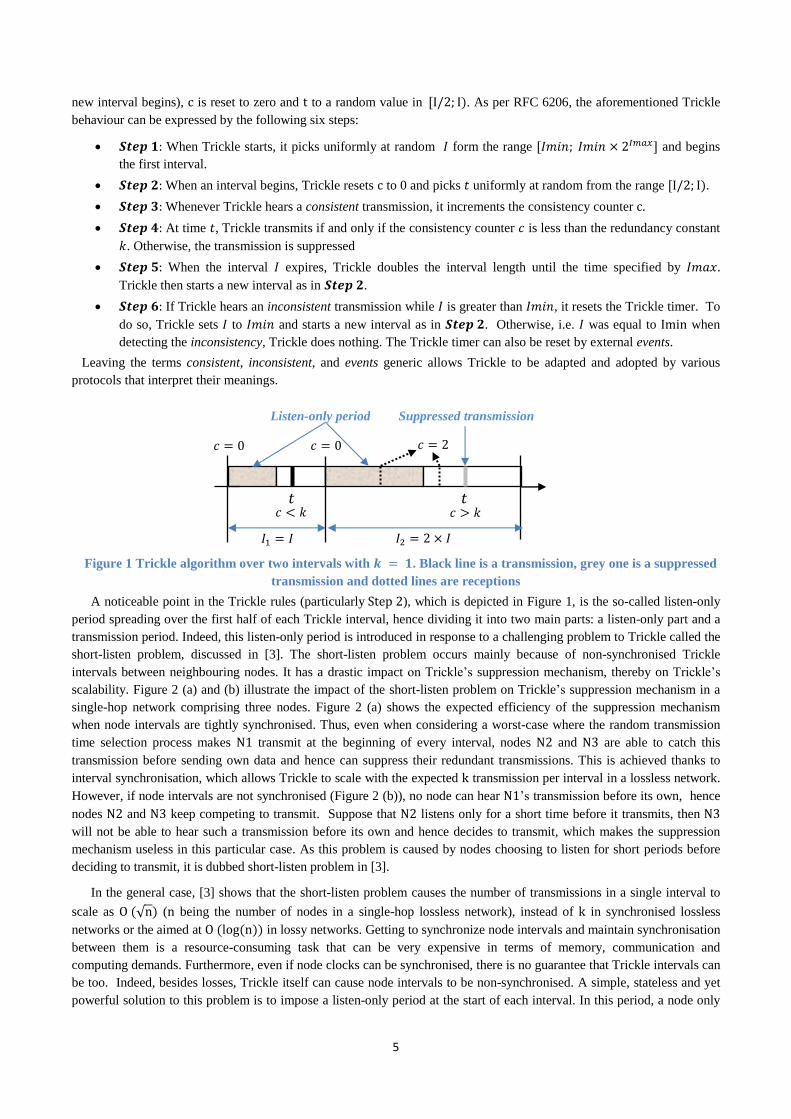
Figure 1 Trickle algorithm over two intervals with 𝒌 = 𝟏. Black line is a transmission, grey one is a suppressed

transmission and dotted lines are receptions

A noticeable point in the Trickle rules (particularly Step 2), which is depicted in Figure 1, is the so-called listen-only

period spreading over the first half of each Trickle interval, hence dividing it into two main parts: a listen-only part and a

transmission period. Indeed, this listen-only period is introduced in response to a challenging problem to Trickle called the

short-listen problem, discussed in [3]. The short-listen problem occurs mainly because of non-synchronised Trickle

intervals between neighbouring nodes. It has a drastic impact on Trickle’s suppression mechanism, thereby on Trickle’s

scalability. Figure 2 (a) and (b) illustrate the impact of the short-listen problem on Trickle’s suppression mechanism in a

single-hop network comprising three nodes. Figure 2 (a) shows the expected efficiency of the suppression mechanism

when node intervals are tightly synchronised. Thus, even when considering a worst-case where the random transmission

time selection process makes N1 transmit at the beginning of every interval, nodes N2 and N3 are able to catch this

transmission before sending own data and hence can suppress their redundant transmissions. This is achieved thanks to

interval synchronisation, which allows Trickle to scale with the expected k transmission per interval in a lossless network.

However, if node intervals are not synchronised (Figure 2 (b)), no node can hear N1’s transmission before its own, hence

nodes N2 and N3 keep competing to transmit. Suppose that N2 listens only for a short time before it transmits, then N3

will not be able to hear such a transmission before its own and hence decides to transmit, which makes the suppression

mechanism useless in this particular case. As this problem is caused by nodes choosing to listen for short periods before

deciding to transmit, it is dubbed short-listen problem in [3].

In the general case, [3] shows that the short-listen problem causes the number of transmissions in a single interval to

scale as O (√n) (n being the number of nodes in a single-hop lossless network), instead of k in synchronised lossless

networks or the aimed at O (log (n)) in lossy networks. Getting to synchronize node intervals and maintain synchronisation

between them is a resource-consuming task that can be very expensive in terms of memory, communication and

computing demands. Furthermore, even if node clocks can be synchronised, there is no guarantee that Trickle intervals can

be too. Indeed, besides losses, Trickle itself can cause node intervals to be non-synchronised. A simple, stateless and yet

powerful solution to this problem is to impose a listen-only period at the start of each interval. In this period, a node only

𝐼1 = 𝐼 𝐼2 = 2 × 𝐼

𝑐 = 0 𝑐 = 0 𝑐 = 2

𝑡 𝑡

Listen-only period

𝑐 > 𝑘 𝑐 < 𝑘

Suppressed transmission

6

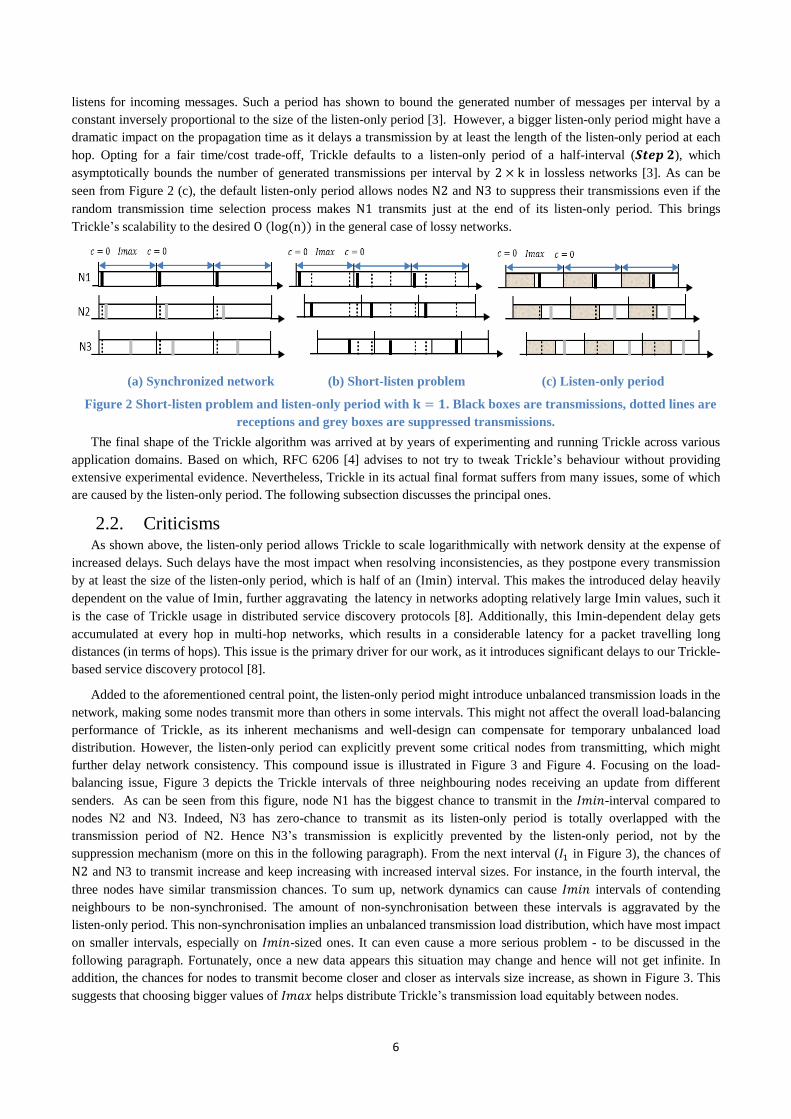
listens for incoming messages. Such a period has shown to bound the generated number of messages per interval by a

constant inversely proportional to the size of the listen-only period [3]. However, a bigger listen-only period might have a

dramatic impact on the propagation time as it delays a transmission by at least the length of the listen-only period at each

hop. Opting for a fair time/cost trade-off, Trickle defaults to a listen-only period of a half-interval (𝑺𝒕𝒆𝒑 𝟐), which

asymptotically bounds the number of generated transmissions per interval by 2 × k in lossless networks [3]. As can be

seen from Figure 2 (c), the default listen-only period allows nodes N2 and N3 to suppress their transmissions even if the

random transmission time selection process makes N1 transmits just at the end of its listen-only period. This brings

Trickle’s scalability to the desired O (log (n)) in the general case of lossy networks.

(a) Synchronized network (b) Short-listen problem (c) Listen-only period

Figure 2 Short-listen problem and listen-only period with 𝐤 = 𝟏. Black boxes are transmissions, dotted lines are

receptions and grey boxes are suppressed transmissions.

The final shape of the Trickle algorithm was arrived at by years of experimenting and running Trickle across various

application domains. Based on which, RFC 6206 [4] advises to not try to tweak Trickle’s behaviour without providing

extensive experimental evidence. Nevertheless, Trickle in its actual final format suffers from many issues, some of which

are caused by the listen-only period. The following subsection discusses the principal ones.

2.2. Criticisms As shown above, the listen-only period allows Trickle to scale logarithmically with network density at the expense of

increased delays. Such delays have the most impact when resolving inconsistencies, as they postpone every transmission

by at least the size of the listen-only period, which is half of an (Imin) interval. This makes the introduced delay heavily

dependent on the value of Imin, further aggravating the latency in networks adopting relatively large Imin values, such it

is the case of Trickle usage in distributed service discovery protocols [8]. Additionally, this Imin-dependent delay gets

accumulated at every hop in multi-hop networks, which results in a considerable latency for a packet travelling long

distances (in terms of hops). This issue is the primary driver for our work, as it introduces significant delays to our Trickle-

based service discovery protocol [8].

Added to the aforementioned central point, the listen-only period might introduce unbalanced transmission loads in the

network, making some nodes transmit more than others in some intervals. This might not affect the overall load-balancing

performance of Trickle, as its inherent mechanisms and well-design can compensate for temporary unbalanced load

distribution. However, the listen-only period can explicitly prevent some critical nodes from transmitting, which might

further delay network consistency. This compound issue is illustrated in Figure 3 and Figure 4. Focusing on the load-

balancing issue, Figure 3 depicts the Trickle intervals of three neighbouring nodes receiving an update from different

senders. As can be seen from this figure, node N1 has the biggest chance to transmit in the 𝐼𝑚𝑖𝑛-interval compared to

nodes N2 and N3. Indeed, N3 has zero-chance to transmit as its listen-only period is totally overlapped with the

transmission period of N2. Hence N3’s transmission is explicitly prevented by the listen-only period, not by the

suppression mechanism (more on this in the following paragraph). From the next interval (𝐼1 in Figure 3), the chances of

N2 and N3 to transmit increase and keep increasing with increased interval sizes. For instance, in the fourth interval, the

three nodes have similar transmission chances. To sum up, network dynamics can cause 𝐼𝑚𝑖𝑛 intervals of contending

neighbours to be non-synchronised. The amount of non-synchronisation between these intervals is aggravated by the

listen-only period. This non-synchronisation implies an unbalanced transmission load distribution, which have most impact

on smaller intervals, especially on 𝐼𝑚𝑖𝑛-sized ones. It can even cause a more serious problem - to be discussed in the

following paragraph. Fortunately, once a new data appears this situation may change and hence will not get infinite. In

addition, the chances for nodes to transmit become closer and closer as intervals size increase, as shown in Figure 3. This

suggests that choosing bigger values of 𝐼𝑚𝑎𝑥 helps distribute Trickle’s transmission load equitably between nodes.

7

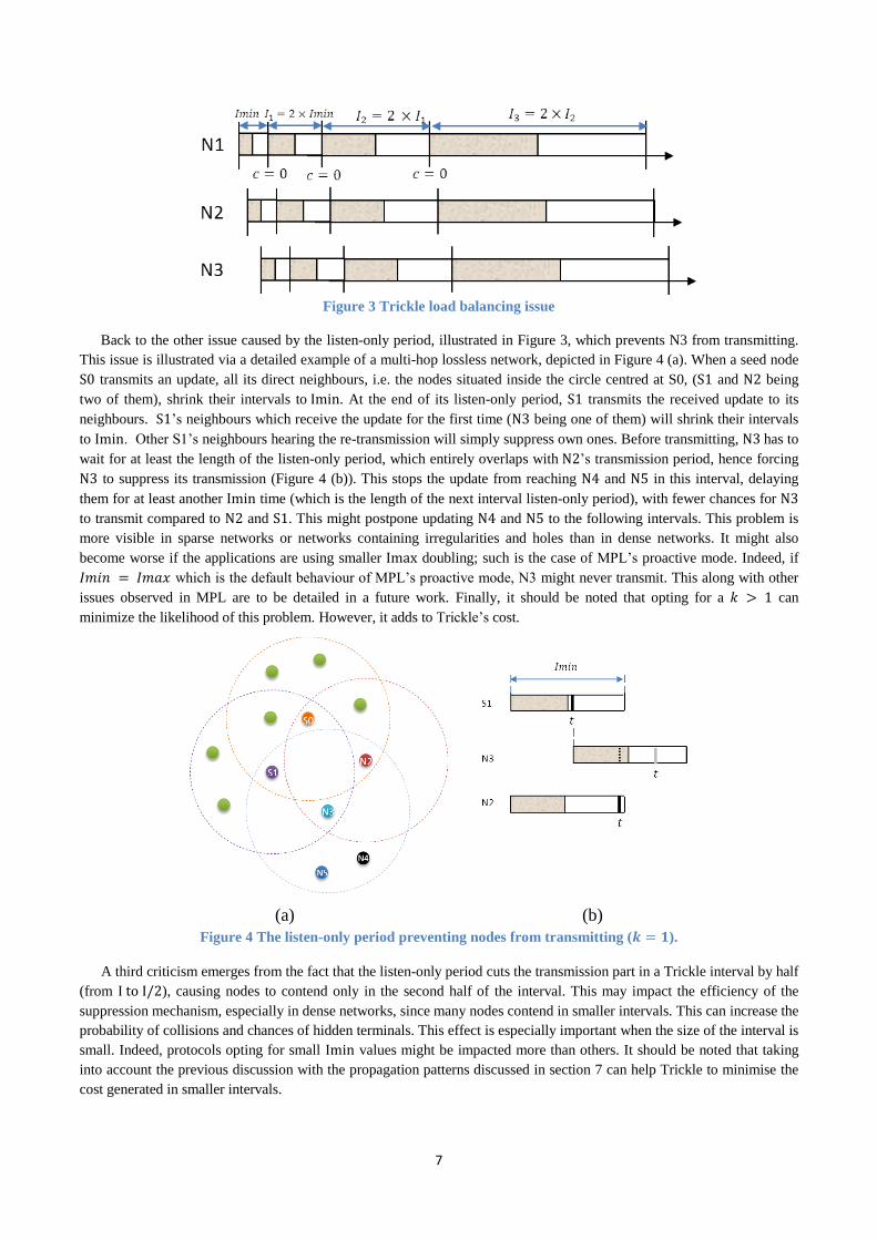
Figure 3 Trickle load balancing issue

Back to the other issue caused by the listen-only period, illustrated in Figure 3, which prevents N3 from transmitting.

This issue is illustrated via a detailed example of a multi-hop lossless network, depicted in Figure 4 (a). When a seed node

S0 transmits an update, all its direct neighbours, i.e. the nodes situated inside the circle centred at S0, (S1 and N2 being

two of them), shrink their intervals to Imin. At the end of its listen-only period, S1 transmits the received update to its

neighbours. S1’s neighbours which receive the update for the first time (N3 being one of them) will shrink their intervals

to Imin. Other S1’s neighbours hearing the re-transmission will simply suppress own ones. Before transmitting, N3 has to

wait for at least the length of the listen-only period, which entirely overlaps with N2’s transmission period, hence forcing

N3 to suppress its transmission (Figure 4 (b)). This stops the update from reaching N4 and N5 in this interval, delaying

them for at least another Imin time (which is the length of the next interval listen-only period), with fewer chances for N3

to transmit compared to N2 and S1. This might postpone updating N4 and N5 to the following intervals. This problem is

more visible in sparse networks or networks containing irregularities and holes than in dense networks. It might also

become worse if the applications are using smaller Imax doubling; such is the case of MPL’s proactive mode. Indeed, if

𝐼𝑚𝑖𝑛 = 𝐼𝑚𝑎𝑥 which is the default behaviour of MPL’s proactive mode, N3 might never transmit. This along with other

issues observed in MPL are to be detailed in a future work. Finally, it should be noted that opting for a 𝑘 > 1 can

minimize the likelihood of this problem. However, it adds to Trickle’s cost.

(a) (b)

Figure 4 The listen-only period preventing nodes from transmitting (𝒌 = 𝟏).

A third criticism emerges from the fact that the listen-only period cuts the transmission part in a Trickle interval by half

(from I to I/2), causing nodes to contend only in the second half of the interval. This may impact the efficiency of the

suppression mechanism, especially in dense networks, since many nodes contend in smaller intervals. This can increase the

probability of collisions and chances of hidden terminals. This effect is especially important when the size of the interval is

small. Indeed, protocols opting for small Imin values might be impacted more than others. It should be noted that taking

into account the previous discussion with the propagation patterns discussed in section 7 can help Trickle to minimise the

cost generated in smaller intervals.

8

In the following sections, we propose a simple, yet very powerful optimisation to Trickle that addresses our criticisms

(especially the main one concerning the propagation time), discuss its impact on Trickle’s cost and scalability, and finally

demonstrate its benefits in respect of the other points discussed above. This is done keeping in mind the recommendations

of RFC 6206 to provide “a great deal of experimental evidence”.

3. The Opt-Trickle Algorithm Having presented an overview of the Trickle algorithm, explained its rationale and discussed our criticisms, we

introduce in this section a simple, yet powerful optimisation to Trickle, which gives birth to the optimised Trickle

algorithm (Opt-Trickle).

3.1. The proposed optimisation Our optimisation is based on a fundamental observation from 𝑆𝑡𝑒𝑝 6 of the Trickle algorithm. 𝑆𝑡𝑒𝑝 6 of Trickle

triggers the nodes receiving an inconsistency to immediately (assuming that receptions occur simultaneously) start new

intervals of size Imin (if 𝐼 > 𝐼𝑚𝑖𝑛). This can present an implicit synchronisation of 𝐼𝑚𝑖𝑛-sized intervals between these

nodes, which comes at no cost and exactly when needed. Such a synchronisation can allow these nodes to choose I from

[0; Imin) without experiencing a short-listen problem with each other. Based on this observation, we propose to modify

𝑆𝑡𝑒𝑝 2 of the Trickle algorithm as follows:

𝑺𝒕𝒆𝒑 𝟐: When an interval begins, Opt-Trickle resets c to 0 and picks 𝑡 uniformly at random from the range:

- [0; 𝐼𝑚𝑖𝑛), if the interval began as a result of 𝑺𝒕𝒆𝒑 𝟔 (because of an inconsistency or in response to external

events).

- [𝐼/2; 𝐼), otherwise (the interval began as a result of 𝑺𝒕𝒆𝒑 𝟏 or 𝑺𝒕𝒆𝒑 𝟓).

Note that neighbours can experience non-synchronised Imin-sized intervals as a result of losses and/or the multi-hop

nature. Fortunately, an implicit synchronisation in the transmission periods of these intervals remains valid, as will be

detailed in section 4. However, there is no guarantee of implicit synchronisation in the following intervals, and hence the

listen-only period is deployed.

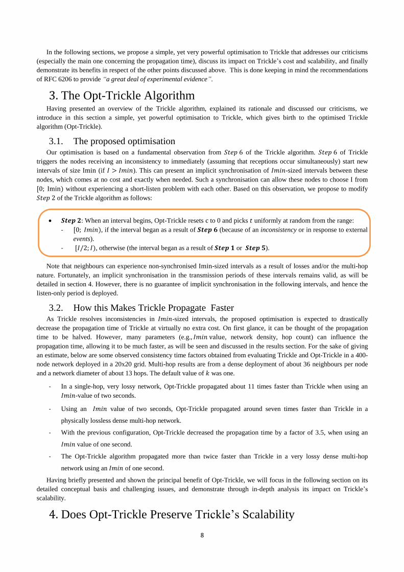
3.2. How this Makes Trickle Propagate Faster As Trickle resolves inconsistencies in 𝐼𝑚𝑖𝑛-sized intervals, the proposed optimisation is expected to drastically

decrease the propagation time of Trickle at virtually no extra cost. On first glance, it can be thought of the propagation

time to be halved. However, many parameters (e.g., 𝐼𝑚𝑖𝑛 value, network density, hop count) can influence the

propagation time, allowing it to be much faster, as will be seen and discussed in the results section. For the sake of giving

an estimate, below are some observed consistency time factors obtained from evaluating Trickle and Opt-Trickle in a 400-

node network deployed in a 20x20 grid. Multi-hop results are from a dense deployment of about 36 neighbours per node

and a network diameter of about 13 hops. The default value of 𝑘 was one.

- In a single-hop, very lossy network, Opt-Trickle propagated about 11 times faster than Trickle when using an

𝐼𝑚𝑖𝑛-value of two seconds.

- Using an 𝐼𝑚𝑖𝑛 value of two seconds, Opt-Trickle propagated around seven times faster than Trickle in a

physically lossless dense multi-hop network.

- With the previous configuration, Opt-Trickle decreased the propagation time by a factor of 3.5, when using an

𝐼𝑚𝑖𝑛 value of one second.

- The Opt-Trickle algorithm propagated more than twice faster than Trickle in a very lossy dense multi-hop

network using an 𝐼𝑚𝑖𝑛 of one second.

Having briefly presented and shown the principal benefit of Opt-Trickle, we will focus in the following section on its

detailed conceptual basis and challenging issues, and demonstrate through in-depth analysis its impact on Trickle’s

scalability.

4. Does Opt-Trickle Preserve Trickle’s Scalability

9

In this section, we discuss Opt-Trickle’s scalability and demonstrate that it preserves Trickle’s logarithmic scalability.

To this end, we start with a simple case of a single-hop lossless network. Then, we relax this assumption by looking at

multi-hop lossless networks and then by introducing losses in single- and multi-hop networks. Note that no assumptions

are made about node interval synchronisations, and hence we opt for the general case of non-synchronised node intervals.

New nodes joining the network are implicitly included in this analysis. Without loss of generality, a Trickle redundancy

constant of one (k = 1) is assumed in the following analysis.

4.1. Lossless, single-hop networks When a node N1 propagates an update in a single-hop lossless network, all other nodes will receive it and, by Trickle’s

𝑆𝑡𝑒𝑝 6, immediately start new Imin-sized intervals (i.e. at the “same” time). This can be considered as an implicit-

synchronisation between these nodes. Hence, the short-listen problem is not be experienced by these nodes if they choose t

from [0; Imin), as shown in Figure 5. Note, however, that whichever receiver transmits (e.g. N2, N3 or N4 in Figure 5) in

the 𝐼𝑚𝑖𝑛 interval, it might experience a short-listen with the second interval of the originator (N1). The impact of this does

not affect Trickle’s scalability, as will be discussed in section 4.5.

This idealistic case shows the basic conceptual building block behind the proposed optimisation. It also clearly

demonstrates that the listen-only period of the 𝐼𝑚𝑖𝑛 interval grows the interval shift between neighbours, for instance,

between the originator (N1) and the other nodes depicted in Figure 5.

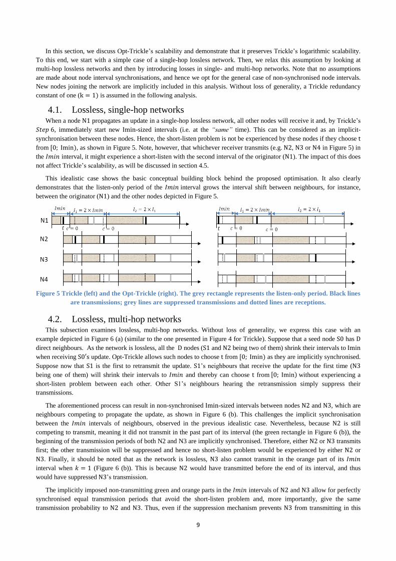
Figure 5 Trickle (left) and the Opt-Trickle (right). The grey rectangle represents the listen-only period. Black lines

are transmissions; grey lines are suppressed transmissions and dotted lines are receptions.

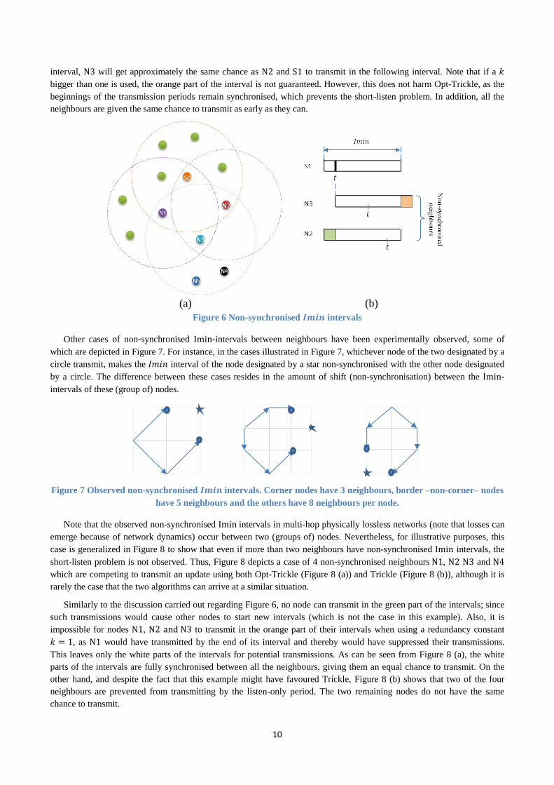
4.2. Lossless, multi-hop networks This subsection examines lossless, multi-hop networks. Without loss of generality, we express this case with an

example depicted in Figure 6 (a) (similar to the one presented in Figure 4 for Trickle). Suppose that a seed node S0 has D

direct neighbours. As the network is lossless, all the D nodes (S1 and N2 being two of them) shrink their intervals to Imin

when receiving S0′s update. Opt-Trickle allows such nodes to choose t from [0; Imin) as they are implicitly synchronised.

Suppose now that S1 is the first to retransmit the update. S1’s neighbours that receive the update for the first time (N3

being one of them) will shrink their intervals to 𝐼𝑚𝑖𝑛 and thereby can choose t from [0; Imin) without experiencing a

short-listen problem between each other. Other S1’s neighbours hearing the retransmission simply suppress their

transmissions.

The aforementioned process can result in non-synchronised Imin-sized intervals between nodes N2 and N3, which are

neighbours competing to propagate the update, as shown in Figure 6 (b). This challenges the implicit synchronisation

between the 𝐼𝑚𝑖𝑛 intervals of neighbours, observed in the previous idealistic case. Nevertheless, because N2 is still

competing to transmit, meaning it did not transmit in the past part of its interval (the green rectangle in Figure 6 (b)), the

beginning of the transmission periods of both N2 and N3 are implicitly synchronised. Therefore, either N2 or N3 transmits

first; the other transmission will be suppressed and hence no short-listen problem would be experienced by either N2 or

N3. Finally, it should be noted that as the network is lossless, N3 also cannot transmit in the orange part of its 𝐼𝑚𝑖𝑛

interval when 𝑘 = 1 (Figure 6 (b)). This is because N2 would have transmitted before the end of its interval, and thus

would have suppressed N3’s transmission.

The implicitly imposed non-transmitting green and orange parts in the 𝐼𝑚𝑖𝑛 intervals of N2 and N3 allow for perfectly

synchronised equal transmission periods that avoid the short-listen problem and, more importantly, give the same

transmission probability to N2 and N3. Thus, even if the suppression mechanism prevents N3 from transmitting in this

10

interval, N3 will get approximately the same chance as N2 and S1 to transmit in the following interval. Note that if a 𝑘

bigger than one is used, the orange part of the interval is not guaranteed. However, this does not harm Opt-Trickle, as the

beginnings of the transmission periods remain synchronised, which prevents the short-listen problem. In addition, all the

neighbours are given the same chance to transmit as early as they can.

(a) (b)

Figure 6 Non-synchronised 𝑰𝒎𝒊𝒏 intervals

Other cases of non-synchronised Imin-intervals between neighbours have been experimentally observed, some of

which are depicted in Figure 7. For instance, in the cases illustrated in Figure 7, whichever node of the two designated by a

circle transmit, makes the 𝐼𝑚𝑖𝑛 interval of the node designated by a star non-synchronised with the other node designated

by a circle. The difference between these cases resides in the amount of shift (non-synchronisation) between the Imin-

intervals of these (group of) nodes.

Figure 7 Observed non-synchronised 𝑰𝒎𝒊𝒏 intervals. Corner nodes have 3 neighbours, border –non-corner– nodes

have 5 neighbours and the others have 8 neighbours per node.

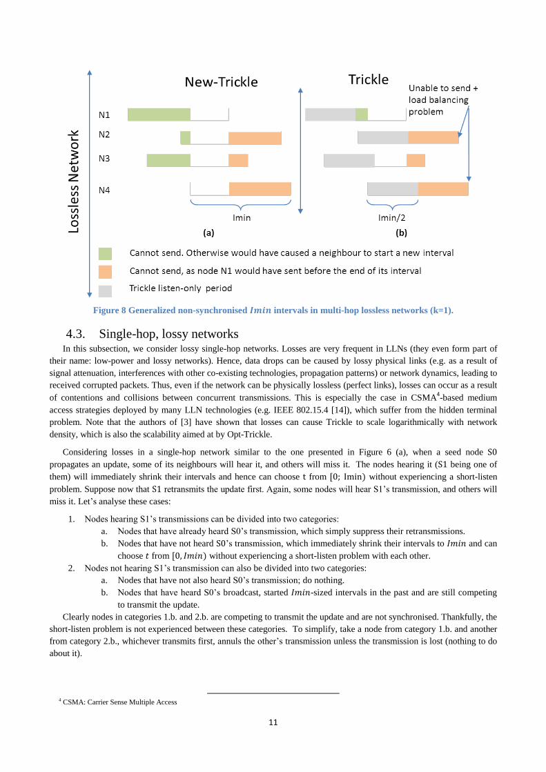
Note that the observed non-synchronised Imin intervals in multi-hop physically lossless networks (note that losses can

emerge because of network dynamics) occur between two (groups of) nodes. Nevertheless, for illustrative purposes, this

case is generalized in Figure 8 to show that even if more than two neighbours have non-synchronised Imin intervals, the

short-listen problem is not observed. Thus, Figure 8 depicts a case of 4 non-synchronised neighbours N1, N2 N3 and N4

which are competing to transmit an update using both Opt-Trickle (Figure 8 (a)) and Trickle (Figure 8 (b)), although it is

rarely the case that the two algorithms can arrive at a similar situation.

Similarly to the discussion carried out regarding Figure 6, no node can transmit in the green part of the intervals; since

such transmissions would cause other nodes to start new intervals (which is not the case in this example). Also, it is

impossible for nodes N1, N2 and N3 to transmit in the orange part of their intervals when using a redundancy constant

𝑘 = 1, as N1 would have transmitted by the end of its interval and thereby would have suppressed their transmissions.

This leaves only the white parts of the intervals for potential transmissions. As can be seen from Figure 8 (a), the white

parts of the intervals are fully synchronised between all the neighbours, giving them an equal chance to transmit. On the

other hand, and despite the fact that this example might have favoured Trickle, Figure 8 (b) shows that two of the four

neighbours are prevented from transmitting by the listen-only period. The two remaining nodes do not have the same

chance to transmit.

11

Figure 8 Generalized non-synchronised 𝑰𝒎𝒊𝒏 intervals in multi-hop lossless networks (k=1).

4.3. Single-hop, lossy networks In this subsection, we consider lossy single-hop networks. Losses are very frequent in LLNs (they even form part of

their name: low-power and lossy networks). Hence, data drops can be caused by lossy physical links (e.g. as a result of

signal attenuation, interferences with other co-existing technologies, propagation patterns) or network dynamics, leading to

received corrupted packets. Thus, even if the network can be physically lossless (perfect links), losses can occur as a result

of contentions and collisions between concurrent transmissions. This is especially the case in CSMA4-based medium

access strategies deployed by many LLN technologies (e.g. IEEE 802.15.4 [14]), which suffer from the hidden terminal

problem. Note that the authors of [3] have shown that losses can cause Trickle to scale logarithmically with network

density, which is also the scalability aimed at by Opt-Trickle.

Considering losses in a single-hop network similar to the one presented in Figure 6 (a), when a seed node S0

propagates an update, some of its neighbours will hear it, and others will miss it. The nodes hearing it (S1 being one of

them) will immediately shrink their intervals and hence can choose t from [0; Imin) without experiencing a short-listen

problem. Suppose now that S1 retransmits the update first. Again, some nodes will hear S1’s transmission, and others will

miss it. Let’s analyse these cases:

1. Nodes hearing S1’s transmissions can be divided into two categories:

a. Nodes that have already heard S0’s transmission, which simply suppress their retransmissions.

b. Nodes that have not heard S0’s transmission, which immediately shrink their intervals to 𝐼𝑚𝑖𝑛 and can

choose 𝑡 from [0, 𝐼𝑚𝑖𝑛) without experiencing a short-listen problem with each other.

2. Nodes not hearing S1’s transmission can also be divided into two categories:

a. Nodes that have not also heard S0’s transmission; do nothing.

b. Nodes that have heard S0’s broadcast, started 𝐼𝑚𝑖𝑛-sized intervals in the past and are still competing

to transmit the update.

Clearly nodes in categories 1.b. and 2.b. are competing to transmit the update and are not synchronised. Thankfully, the

short-listen problem is not experienced between these categories. To simplify, take a node from category 1.b. and another

from category 2.b., whichever transmits first, annuls the other’s transmission unless the transmission is lost (nothing to do

about it).

4 CSMA: Carrier Sense Multiple Access

12

To generalize this case, let’s suppose a single-hop network in which M non-synchronised (group of) nodes are

competing to transmit a previously received update. The remaining nodes in the network are denoted by R. We examine in

the following points what happens, in the M and R sets, when a first node N1 from M transmits.

1. Suppose that 𝐻 nodes from 𝑀 will hear N1’s transmission, hence they suppress their transmissions.

2. The remaining 𝑀 − 𝐻 − 1 nodes from 𝑀 will miss it; hence they continue competing to propagate the update as

they have missed it due to the lossy nature of the network.

3. Now consider that 𝐿 nodes from 𝑅 have heard the update for the first time. They start new 𝐼𝑚𝑖𝑛-sized intervals

and they will be competing with the 𝑀 − 𝐻 − 1 nodes to propagate it.

4. The remaining 𝑅 − 𝐿 nodes, which either did not hear N1’s transmission because of the lossy nature of the

network or they are already aware of the update, keep quiet.

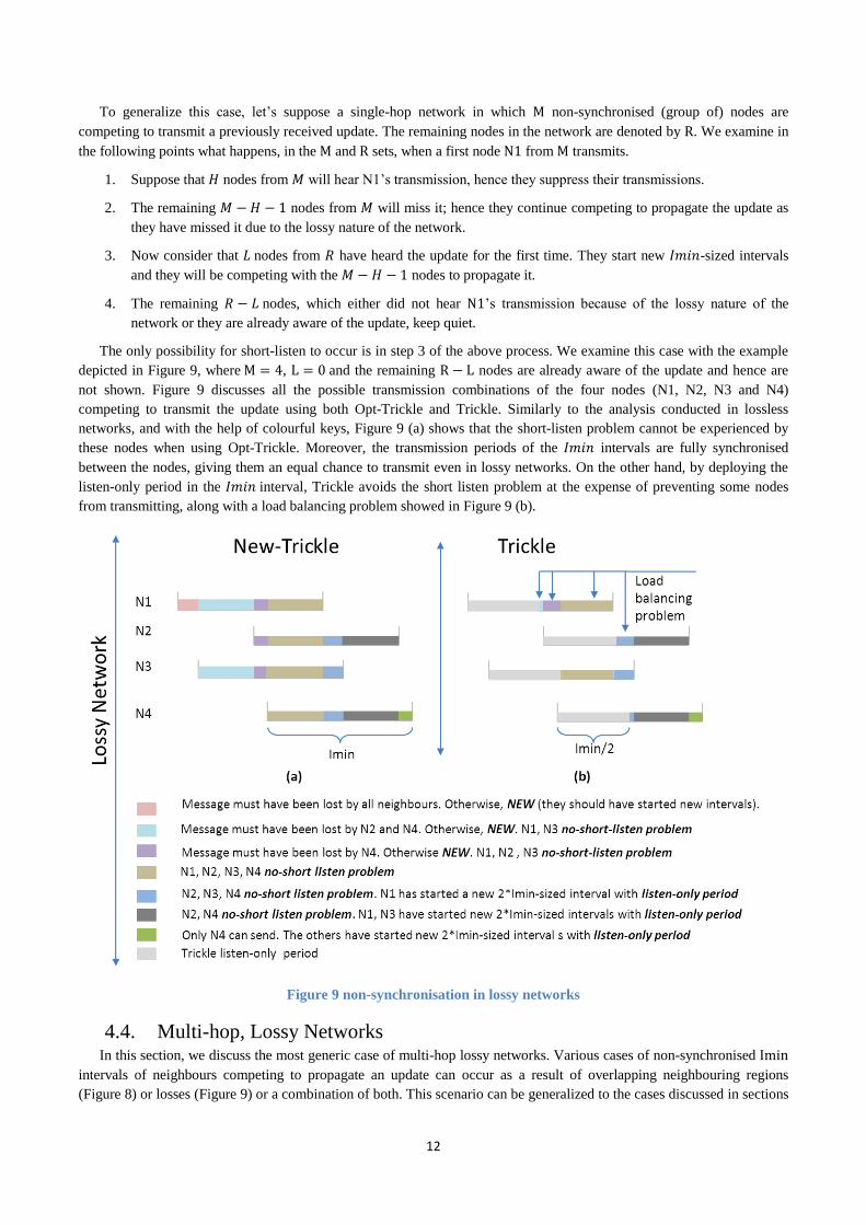
The only possibility for short-listen to occur is in step 3 of the above process. We examine this case with the example

depicted in Figure 9, where M = 4, L = 0 and the remaining R − L nodes are already aware of the update and hence are

not shown. Figure 9 discusses all the possible transmission combinations of the four nodes (N1, N2, N3 and N4)

competing to transmit the update using both Opt-Trickle and Trickle. Similarly to the analysis conducted in lossless

networks, and with the help of colourful keys, Figure 9 (a) shows that the short-listen problem cannot be experienced by

these nodes when using Opt-Trickle. Moreover, the transmission periods of the 𝐼𝑚𝑖𝑛 intervals are fully synchronised

between the nodes, giving them an equal chance to transmit even in lossy networks. On the other hand, by deploying the

listen-only period in the 𝐼𝑚𝑖𝑛 interval, Trickle avoids the short listen problem at the expense of preventing some nodes

from transmitting, along with a load balancing problem showed in Figure 9 (b).

Figure 9 non-synchronisation in lossy networks

4.4. Multi-hop, Lossy Networks In this section, we discuss the most generic case of multi-hop lossy networks. Various cases of non-synchronised Imin

intervals of neighbours competing to propagate an update can occur as a result of overlapping neighbouring regions

(Figure 8) or losses (Figure 9) or a combination of both. This scenario can be generalized to the cases discussed in sections

13

4.2 and 4.3. For instance, if one supposes that losses do not occur in the Imin-sized intervals, then such a situation is

encapsulated in the generalised scenario depicted in Figure 8. Otherwise, the interactions between neighbours can be

captured by the generic case of losses illustrated in Figure 9. Fortunately, in both cases, Opt-Trickle does not only avoid

the short-listen problem but also ensures a perfect synchronisation in the transmission periods of the Imin-sized intervals.

4.5. The Big Picture Having shown that Opt-Trickle does not suffer from the short-listen problem in Imin-sized intervals, we put these

intervals in the larger context of Trickle’s behaviour and determine whether Opt-Trickle preserves the scalability and

robustness of Trickle.

We start with the example of a perfect lossless single-hop network, depicted in Figure 5 (section 4.1). This example

shows that Trickle deliberately prevents the originator node N1 from transmitting in the second interval (I1 interval in

Figure 5), as the transmission of N2, N3 or N4 in the Imin-interval forcibly coincides with the listen-only period of the

second interval of N1. However, Opt-Trickle does not guarantee that N2, N3 or N4 transmission in the Imin-interval falls

in the second interval of the originator node and hence such a transmission might experience a short-listen problem with

I1′s interval of N1. Nevertheless, while Opt-Trickle allows all the nodes to transmit in the second interval, instead of only

N2, N3 or N4 in the case of Trickle, the number of transmissions in the second interval is 𝑘 for both algorithms.

Fortunately, in this lossless perfect scenario, both algorithms generate the same cost, with the advantage of equitable

transmission chances provided by Opt-Trickle.

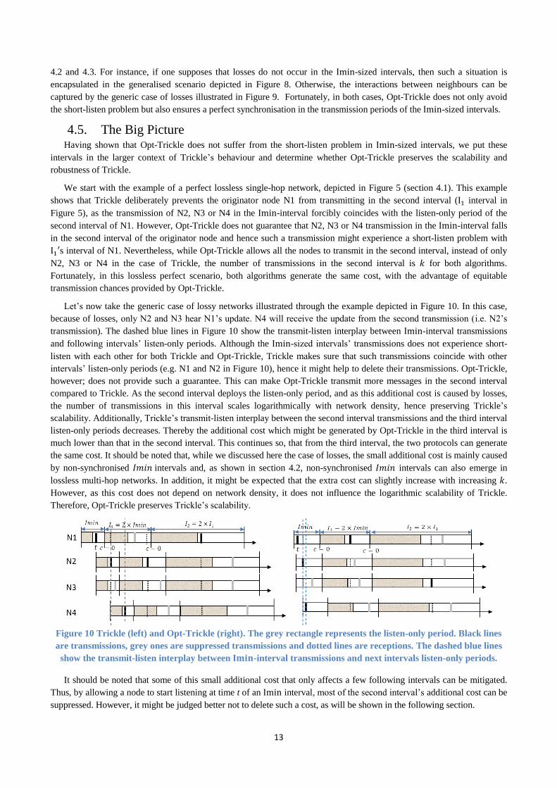
Let’s now take the generic case of lossy networks illustrated through the example depicted in Figure 10. In this case,

because of losses, only N2 and N3 hear N1’s update. N4 will receive the update from the second transmission (i.e. N2’s

transmission). The dashed blue lines in Figure 10 show the transmit-listen interplay between Imin-interval transmissions

and following intervals’ listen-only periods. Although the Imin-sized intervals’ transmissions does not experience short-

listen with each other for both Trickle and Opt-Trickle, Trickle makes sure that such transmissions coincide with other

intervals’ listen-only periods (e.g. N1 and N2 in Figure 10), hence it might help to delete their transmissions. Opt-Trickle,

however; does not provide such a guarantee. This can make Opt-Trickle transmit more messages in the second interval

compared to Trickle. As the second interval deploys the listen-only period, and as this additional cost is caused by losses,

the number of transmissions in this interval scales logarithmically with network density, hence preserving Trickle’s

scalability. Additionally, Trickle’s transmit-listen interplay between the second interval transmissions and the third interval

listen-only periods decreases. Thereby the additional cost which might be generated by Opt-Trickle in the third interval is

much lower than that in the second interval. This continues so, that from the third interval, the two protocols can generate

the same cost. It should be noted that, while we discussed here the case of losses, the small additional cost is mainly caused

by non-synchronised 𝐼𝑚𝑖𝑛 intervals and, as shown in section 4.2, non-synchronised 𝐼𝑚𝑖𝑛 intervals can also emerge in

lossless multi-hop networks. In addition, it might be expected that the extra cost can slightly increase with increasing 𝑘.

However, as this cost does not depend on network density, it does not influence the logarithmic scalability of Trickle.

Therefore, Opt-Trickle preserves Trickle’s scalability.

Figure 10 Trickle (left) and Opt-Trickle (right). The grey rectangle represents the listen-only period. Black lines

are transmissions, grey ones are suppressed transmissions and dotted lines are receptions. The dashed blue lines

show the transmit-listen interplay between 𝐈𝐦𝐢𝐧-interval transmissions and next intervals listen-only periods.

It should be noted that some of this small additional cost that only affects a few following intervals can be mitigated.

Thus, by allowing a node to start listening at time t of an Imin interval, most of the second interval’s additional cost can be

suppressed. However, it might be judged better not to delete such a cost, as will be shown in the following section.

14

Having demonstrated that the proposed optimisation does not influence Trickle’s scalability, we present in the

following section some other expected benefits of Opt-Trickle.

5. Expected Other Benefits of Opt-Trickle In previous sections, we showed that choosing t from [0; Imin) can allow Opt-Trickle to propagate dramatically faster

without resulting in a short-listen problem between competing neighbours. We also demonstrated that although a small

additional cost can occur in Opt-Trickle, this cost might only be observed in a few (e.g. 2-3) intervals following 𝐼𝑚𝑖𝑛, and

that it does not influence Trickle’s scalability. In this section, we outline some other benefits that can result from Opt-

Trickle, which address the remaining criticisms discussed in section 2.2.

5.1. Load Balancing Trickle inherits a balanced load distribution arising from the uniform random choice of transmission time. However,

this balanced load can be challenged by the listen-only period as explained in section 2.2. As shown in that section,

unbalanced load distribution has more chances to occur in small intervals (especially Imin-sized intervals), where it has the

most impact. Additionally, it was shown in section 2.2 that the listen-only period of Imin-intervals may explicitly stop

some transmissions, thus preventing parts of the network from being quickly updated. Throughout the above analysis

(section 4), we showed that Opt-Trickle gives all competing nodes similar chances to transmit an update, which allows it to

solve this serious issue. In what follows, we focus on how Opt-Trickle helps to bring a balanced load distribution. To this

end, we use the generic case of lossy networks depicted in Figure 10.

As can be seen from Figure 10, Trickle imposes on every node to wait for at least the size of the listen-only period

before propagating an update. This shifts the intervals of the receivers by at least Imin / 2 from the originator. A receiver

form those (e.g. node N2 in Figure 10) has to wait for at least another Imin / 2 before transmitting. As a result, a receiver

of such an update (for instance, node N4 in Figure 10) is again shifted by at least Imin / 2 from N2 and by Imin from the

seed. This process gets aggravated under heavy losses, which adds to the interval skew between neighbours. While this

behaviour gives Trickle a wavelike propagation as will be seen in section 7, it might give some nodes more chances to

transmit in the following intervals, as discussed in section 2.2. Opt-Trickle, however, does not impose any restriction on

nodes competing to transmit an update. Hence, in addition to giving competing nodes the same chances to send, it allows

for a smaller interval skew between neighbours, as shown in Figure 10.

To see the impact of the above in practice, we conducted an experiment in TOSSIM. We deployed a Trickle

application (similar to Setup 1 described later-on in section 8) in a sparse grid topology of 15 × 15 nodes. The topology

and link configurations are those of 15-15-sparse-mica2-grid.txt5 example available in TOSSIM. We used an artificial

noise of -115 dBm to feed the Closest-fit Pattern Matching (CPM) model used by TOSSIM [15]. We measured the

standard deviation of the number of transmissions per node as a metric of the load balancing: the smallest the standard

deviation the better balanced the transmission loads. Obtained results are presented in Table 1. As can be seen from this

table, both Trickle and Opt-Trickle try to provide a balanced load distribution between nodes. Opt-Trickle provides better

load balancing than Trickle for both small and big values of Imin with the biggest gap observed with small Imin values.

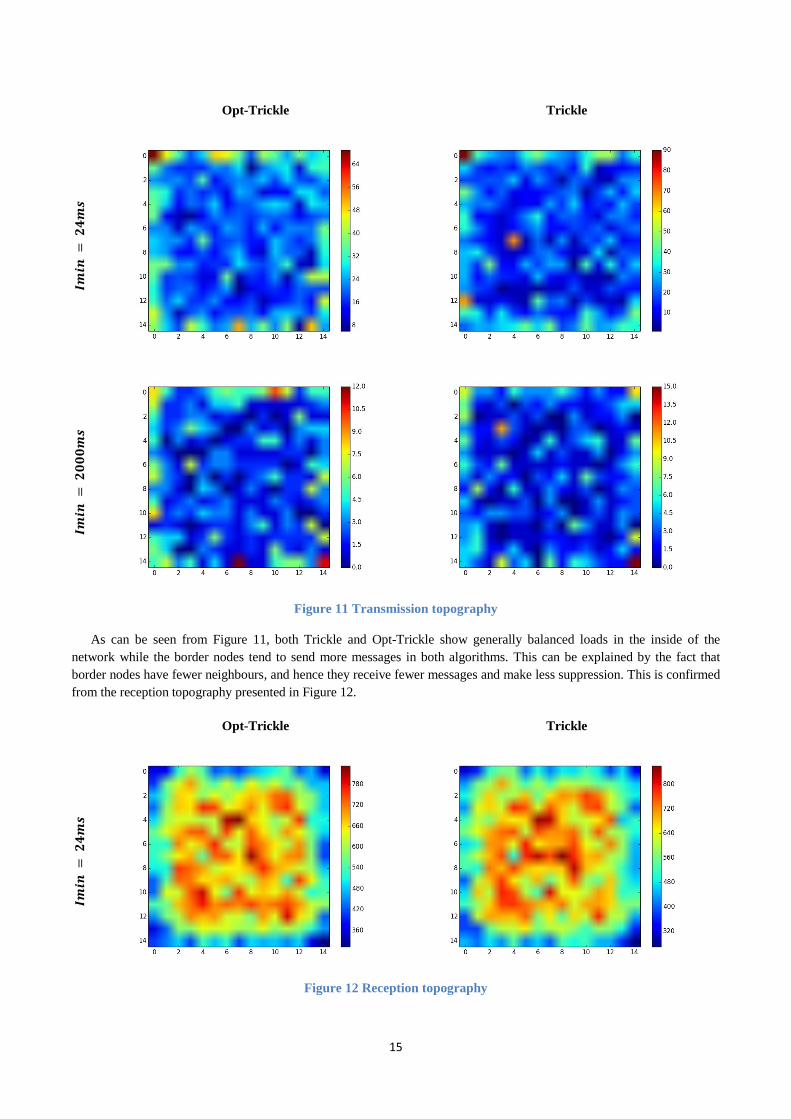
This confirms our assertions in the above discussion. To further get a feel on the dispersion of transmissions between

nodes, we present in Figure 11 the transmission topography of Trickle and Opt-Trickle for both values of 𝐼𝑚𝑖𝑛 presented

in Table 1. Note that all the topographies given below are the result of one typical execution.

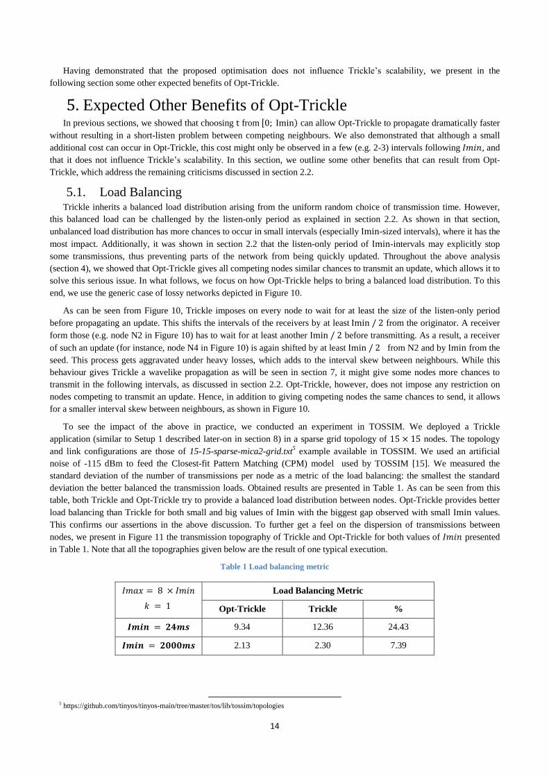
Table 1 Load balancing metric

𝐼𝑚𝑎𝑥 = 8 × 𝐼𝑚𝑖𝑛

𝑘 = 1

Load Balancing Metric

Opt-Trickle Trickle %

𝑰𝒎𝒊𝒏 = 𝟐𝟒𝒎𝒔 9.34 12.36 24.43

𝑰𝒎𝒊𝒏 = 𝟐𝟎𝟎𝟎𝒎𝒔 2.13 2.30 7.39

5 https://github.com/tinyos/tinyos-main/tree/master/tos/lib/tossim/topologies

15

Opt-Trickle Trickle

𝑰𝒎𝒊𝒏

= 𝟐

𝟒𝒎

𝒔

𝑰𝒎𝒊𝒏

=

𝟐𝟎

𝟎𝟎

𝒎𝒔

Figure 11 Transmission topography

As can be seen from Figure 11, both Trickle and Opt-Trickle show generally balanced loads in the inside of the

network while the border nodes tend to send more messages in both algorithms. This can be explained by the fact that

border nodes have fewer neighbours, and hence they receive fewer messages and make less suppression. This is confirmed

from the reception topography presented in Figure 12.

Opt-Trickle Trickle

𝑰𝒎𝒊𝒏

= 𝟐

𝟒𝒎

𝒔

Figure 12 Reception topography

16

5.2. Potentially Less Inconsistent Transmissions Obtained results in section 9 showed that generally Opt-Trickle generates less inconsistent messages than Trickle. This

was observed especially if the network spans a long number of hops. In such a case, it was also shown that the gap in the

number of inconsistent messages generated by Opt-Trickle and Trickle increases with increasing values of 𝑘. In order to

try to explaining such results, this section makes the following observations:

- Opt-Trickle showed a perfect synchronisation in the transmission periods of the Imin-intervals of neighbours

competing to propagate an update (Figure 8 and Figure 9). Therefore, Opt-Trickle can theoretically ensure the

expected number of 𝑘 transmission per an 𝐼𝑚𝑖𝑛 interval in lossless networks (𝑘 × 𝑙𝑜𝑔 (𝑛) in lossy networks)

when 𝑘 = 1. For the other values of 𝑘, there might be a higher probability to approach the theoretical limit.

- Having the gap in the number of inconsistent transmissions more observable when the message travels long

distances (in terms of hops) and with increasing values of 𝑘 can be caused by the propagation patterns of both

algorithms which will be discussed in section 7.

- However, as discussed in section 2.2, the listen-only period of the 𝐼𝑚𝑖𝑛-interval in Trickle can prevent a node

from transmitting in this interval, especially when using a redundancy constant 𝑘 = 1. This fact might allow

Trickle to generate fewer messages in an 𝐼𝑚𝑖𝑛 interval for such a value of 𝑘 in some scenarios.

These observations suggest that more analysis is required to fully understand the drivers behind the observed

behaviours. Such an analysis can start from the propagation patterns discussed in section 7 that gives insights on how the

propagation in the 𝐼𝑚𝑖𝑛 interval behaves in both Trickle and Opt-Trickle.

5.3. More Room for Contentions Doubling the size of the potential transmission part of an 𝐼𝑚𝑖𝑛 interval can give nodes more time for contentions,

which helps to minimise the probability of collisions and hidden terminals. Therefore, Opt-Trickle might improve the

performance of the suppression mechanism. This is especially important when opting for very small 𝐼𝑚𝑖𝑛 intervals or/and

deploying Opt-Trickle in dense networks. However, since Opt-Trickle ensures similar chances for nodes to transmit in an

𝐼𝑚𝑖𝑛-Interval, whilst Trickle explicitly prevents some nodes from transmitting, Trickle can still, in some cases, generate

less overhead in an 𝐼𝑚𝑖𝑛 interval. Also, the propagation pattern of Trickle discussed in section 7 ensures a progressive

wavelike propagation which only allows fewer nodes to contend. This in turns help minimising collisions and hidden

terminals. Again this observation suggests thorough analysis which is left for future work.

6. More Optimizations Having presented Opt-Trickle, discussed its benefits, trade-offs and scalability, this section introduces some subsequent

optimisations aiming to enhance its latency further.

6.1. Optimized Short-Trickle (OS-Trickle) OS-Trickle does not improve on Opt-Trickle’s cost, but it seems to present a better solution in terms of latency as it

always takes t from [0; I) similarly to Short-Trickle and addresses the short-listen problem in an interesting way.

Since the short-listen problem is caused by nodes choosing to listen for only a short period before deciding to transmit,

OS-Trickle takes another approach to addressing it. Thus, it allows nodes to have short-listen in the first interval and then

asks them to start listening at time t in order to avoid short-listen in the following intervals. Thus, this idea allows next

intervals to learn from previous unnecessary gossips. OS-Trickle follows a ‘be polite’ strategy similar to this: if a node did

not take enough time to listen before deciding to speak, it is asked to listen carefully in the remaining time in order to make

a better decision next time (in the following interval).

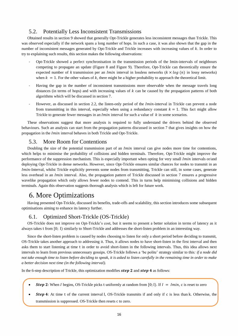
In the 6-step description of Trickle, this optimization modifies 𝒔𝒕𝒆𝒑 𝟐 and 𝒔𝒕𝒆𝒑 𝟒 as follows:

𝑺𝒕𝒆𝒑 𝟐: When 𝐼 begins, OS-Trickle picks t uniformly at random from [0; I). If 𝐼 = 𝐼𝑚𝑖𝑛, c is reset to zero

𝑺𝒕𝒆𝒑 𝟒: At time t of the current interval I, OS-Trickle transmits if and only if c is less than k. Otherwise, the

transmission is suppressed. OS-Trickle then resets c to zero.

17

At a first glance, OS-Trickle seems to solve the short-listen problem. However, with a closer look, a short-listen gap

can still be observed. In order to quantify the impact of the short-listen gap on OS-Trickle, we carried out experiments in

the maintenance mode (all nodes have initially the same information) with an 𝐼𝑚𝑎𝑥 = 1 𝑠𝑒𝑐𝑜𝑛𝑑, in both Cooja/MSPSim

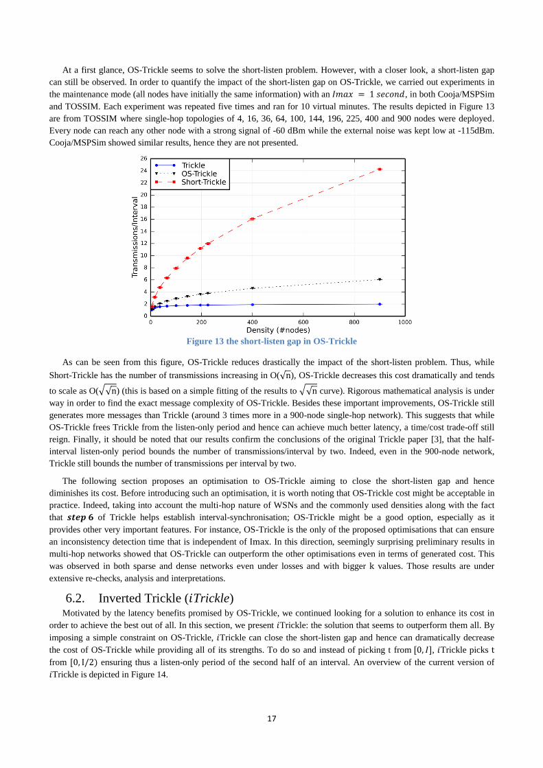
and TOSSIM. Each experiment was repeated five times and ran for 10 virtual minutes. The results depicted in Figure 13

are from TOSSIM where single-hop topologies of 4, 16, 36, 64, 100, 144, 196, 225, 400 and 900 nodes were deployed.

Every node can reach any other node with a strong signal of -60 dBm while the external noise was kept low at -115dBm.

Cooja/MSPSim showed similar results, hence they are not presented.

Figure 13 the short-listen gap in OS-Trickle

As can be seen from this figure, OS-Trickle reduces drastically the impact of the short-listen problem. Thus, while

Short-Trickle has the number of transmissions increasing in O(√n), OS-Trickle decreases this cost dramatically and tends

to scale as O(√√n) (this is based on a simple fitting of the results to √√n curve). Rigorous mathematical analysis is under

way in order to find the exact message complexity of OS-Trickle. Besides these important improvements, OS-Trickle still

generates more messages than Trickle (around 3 times more in a 900-node single-hop network). This suggests that while

OS-Trickle frees Trickle from the listen-only period and hence can achieve much better latency, a time/cost trade-off still

reign. Finally, it should be noted that our results confirm the conclusions of the original Trickle paper [3], that the half-

interval listen-only period bounds the number of transmissions/interval by two. Indeed, even in the 900-node network,

Trickle still bounds the number of transmissions per interval by two.

The following section proposes an optimisation to OS-Trickle aiming to close the short-listen gap and hence

diminishes its cost. Before introducing such an optimisation, it is worth noting that OS-Trickle cost might be acceptable in

practice. Indeed, taking into account the multi-hop nature of WSNs and the commonly used densities along with the fact

that 𝒔𝒕𝒆𝒑 𝟔 of Trickle helps establish interval-synchronisation; OS-Trickle might be a good option, especially as it

provides other very important features. For instance, OS-Trickle is the only of the proposed optimisations that can ensure

an inconsistency detection time that is independent of Imax. In this direction, seemingly surprising preliminary results in

multi-hop networks showed that OS-Trickle can outperform the other optimisations even in terms of generated cost. This

was observed in both sparse and dense networks even under losses and with bigger k values. Those results are under

extensive re-checks, analysis and interpretations.

6.2. Inverted Trickle (𝑖Trickle) Motivated by the latency benefits promised by OS-Trickle, we continued looking for a solution to enhance its cost in

order to achieve the best out of all. In this section, we present 𝑖Trickle: the solution that seems to outperform them all. By

imposing a simple constraint on OS-Trickle, 𝑖Trickle can close the short-listen gap and hence can dramatically decrease

the cost of OS-Trickle while providing all of its strengths. To do so and instead of picking t from [0, 𝐼], 𝑖Trickle picks t

from [0, I/2) ensuring thus a listen-only period of the second half of an interval. An overview of the current version of

𝑖Trickle is depicted in Figure 14.

18

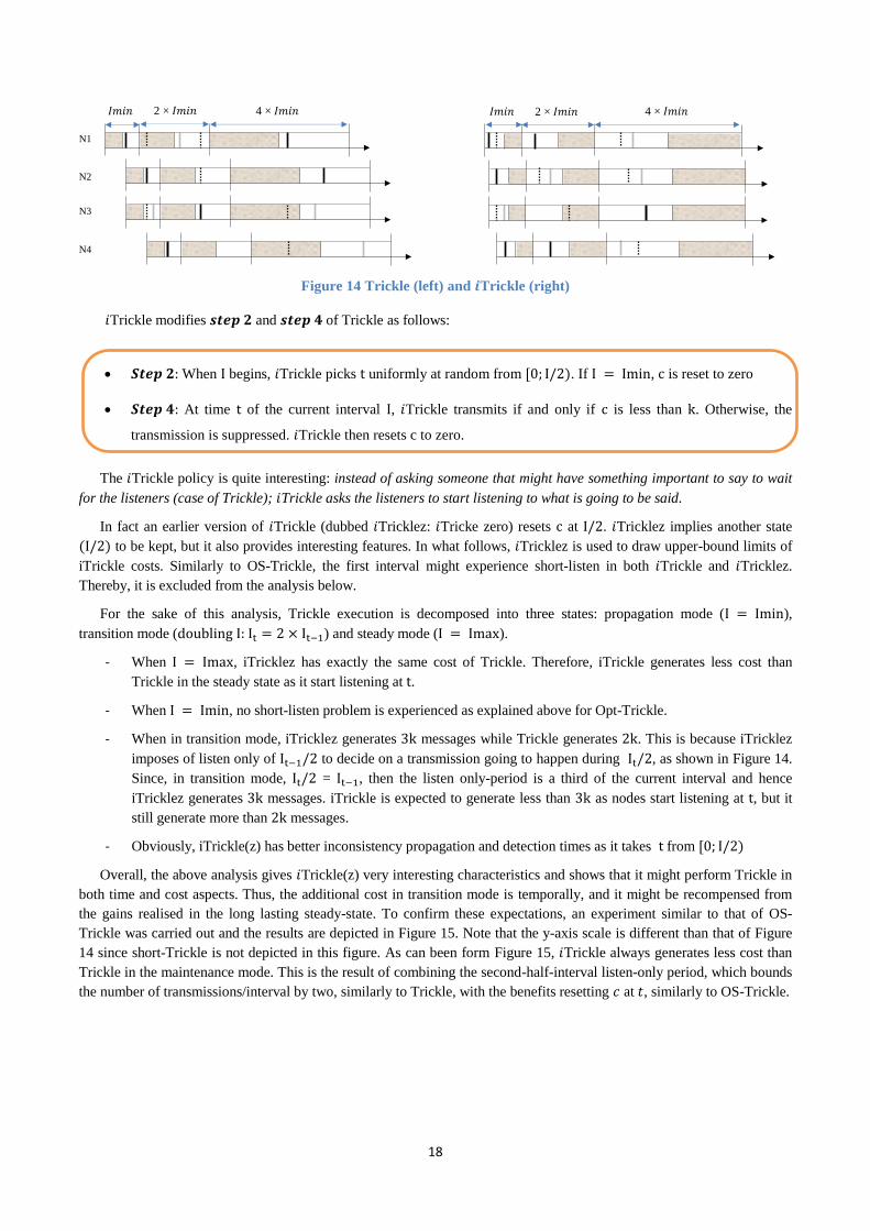
Figure 14 Trickle (left) and 𝒊Trickle (right)

𝑖Trickle modifies 𝒔𝒕𝒆𝒑 𝟐 and 𝒔𝒕𝒆𝒑 𝟒 of Trickle as follows:

𝑺𝒕𝒆𝒑 𝟐: When I begins, 𝑖Trickle picks t uniformly at random from [0; I/2). If I = Imin, c is reset to zero

𝑺𝒕𝒆𝒑 𝟒: At time t of the current interval I, 𝑖Trickle transmits if and only if c is less than k. Otherwise, the

transmission is suppressed. 𝑖Trickle then resets c to zero.

The 𝑖Trickle policy is quite interesting: instead of asking someone that might have something important to say to wait

for the listeners (case of Trickle); 𝑖Trickle asks the listeners to start listening to what is going to be said.

In fact an earlier version of 𝑖Trickle (dubbed 𝑖Tricklez: 𝑖Tricke zero) resets c at I/2. 𝑖Tricklez implies another state

(I/2) to be kept, but it also provides interesting features. In what follows, 𝑖Tricklez is used to draw upper-bound limits of

iTrickle costs. Similarly to OS-Trickle, the first interval might experience short-listen in both 𝑖Trickle and 𝑖Tricklez.

Thereby, it is excluded from the analysis below.

For the sake of this analysis, Trickle execution is decomposed into three states: propagation mode (I = Imin),

transition mode (doubling I: It = 2 × It−1) and steady mode (I = Imax).

- When I = Imax, iTricklez has exactly the same cost of Trickle. Therefore, iTrickle generates less cost than

Trickle in the steady state as it start listening at t.

- When I = Imin, no short-listen problem is experienced as explained above for Opt-Trickle.

- When in transition mode, iTricklez generates 3k messages while Trickle generates 2k. This is because iTricklez

imposes of listen only of It−1/2 to decide on a transmission going to happen during It/2, as shown in Figure 14.

Since, in transition mode, It/2 = It−1, then the listen only-period is a third of the current interval and hence

iTricklez generates 3k messages. iTrickle is expected to generate less than 3k as nodes start listening at t, but it

still generate more than 2k messages.

- Obviously, iTrickle(z) has better inconsistency propagation and detection times as it takes t from [0; I/2)

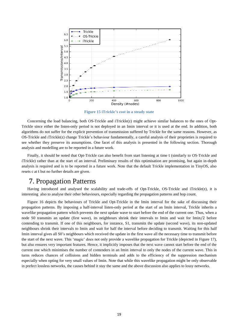
Overall, the above analysis gives 𝑖Trickle(z) very interesting characteristics and shows that it might perform Trickle in

both time and cost aspects. Thus, the additional cost in transition mode is temporally, and it might be recompensed from

the gains realised in the long lasting steady-state. To confirm these expectations, an experiment similar to that of OS-

Trickle was carried out and the results are depicted in Figure 15. Note that the y-axis scale is different than that of Figure

14 since short-Trickle is not depicted in this figure. As can been form Figure 15, 𝑖Trickle always generates less cost than

Trickle in the maintenance mode. This is the result of combining the second-half-interval listen-only period, which bounds

the number of transmissions/interval by two, similarly to Trickle, with the benefits resetting 𝑐 at 𝑡, similarly to OS-Trickle.

N2

N3

N4

N1

𝐼𝑚𝑖𝑛 2 × 𝐼𝑚𝑖𝑛 4 × 𝐼𝑚𝑖𝑛

𝐼𝑚𝑖𝑛 2 × 𝐼𝑚𝑖𝑛 4 × 𝐼𝑚𝑖𝑛

19

Figure 15 iTrickle’s cost in a steady state

Concerning the load balancing, both OS-Trickle and 𝑖Trickle(z) might achieve similar balances to the ones of Opt-

Trickle since either the listen-only period is not deployed in an Imin interval or it is used at the end. In addition, both

algorithms do not suffer for the explicit prevention of transmission suffered by Trickle for the same reasons. However, as

OS-Trickle and 𝑖Trickle(z) change Trickle’s behaviour fundamentally, a careful analysis of their proprieties is required to

see whether they preserve its assumptions. One facet of this analysis is presented in the following section. Thorough

analysis and modelling are to be reported in a future work.

Finally, it should be noted that Opt-Trickle can also benefit from start listening at time t (similarly to OS-Trickle and

𝑖Trickle) rather than at the start of an interval. Preliminary results of this optimisation are promising, but again in-depth

analysis is required and is to be reported in a future work. Note that the default Trickle implementation in TinyOS, also

resets c at t but no further details are given.

7. Propagation Patterns Having introduced and analysed the scalability and trade-offs of Opt-Trickle, OS-Trickle and iTrickle(z), it is

interesting also to analyse their other behaviours, especially regarding the propagation patterns and hop count.

Figure 16 depicts the behaviours of Trickle and Opt-Trickle in the Imin interval for the sake of discussing their

propagation patterns. By imposing a half-interval listen-only period at the start of an Imin interval, Trickle inherits a

wavelike propagation pattern which prevents the next update wave to start before the end of the current one. Thus, when a

node S0 transmits an update (first wave), its neighbours shrink their intervals to Imin and wait for Imin/2 before

contending to transmit. If one of this neighbours, for instance, S1, transmits the update (second wave), its non-updated

neighbours shrink their intervals to Imin and wait for half the interval before deciding to transmit. Waiting for this half

Imin interval gives all S0’s neighbours which received the update in the first wave all the necessary time to transmit before

the start of the next wave. This ‘magic’ does not only provide a wavelike propagation for Trickle (depicted in Figure 17),

but also ensures very important features. Hence, it implicitly imposes that the next wave cannot start before the end of the

current one which minimises the number of contenders in an Imin interval to only the nodes of the current wave. This in

turns reduces chances of collisions and hidden terminals and adds to the efficiency of the suppression mechanism

especially when opting for very small values of Imin. Note that while this wavelike propagation might be only observable

in prefect lossless networks, the causes behind it stay the same and the above discussion also applies to lossy networks.

20

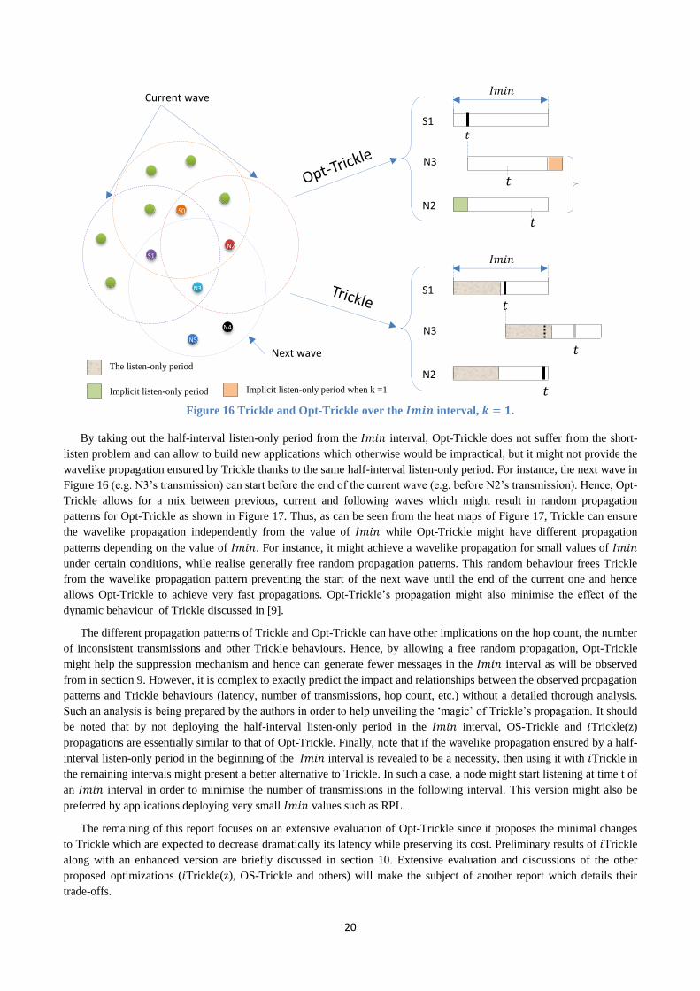
Figure 16 Trickle and Opt-Trickle over the 𝑰𝒎𝒊𝒏 interval, 𝒌 = 𝟏.

By taking out the half-interval listen-only period from the 𝐼𝑚𝑖𝑛 interval, Opt-Trickle does not suffer from the short-

listen problem and can allow to build new applications which otherwise would be impractical, but it might not provide the

wavelike propagation ensured by Trickle thanks to the same half-interval listen-only period. For instance, the next wave in

Figure 16 (e.g. N3’s transmission) can start before the end of the current wave (e.g. before N2’s transmission). Hence, Opt-

Trickle allows for a mix between previous, current and following waves which might result in random propagation

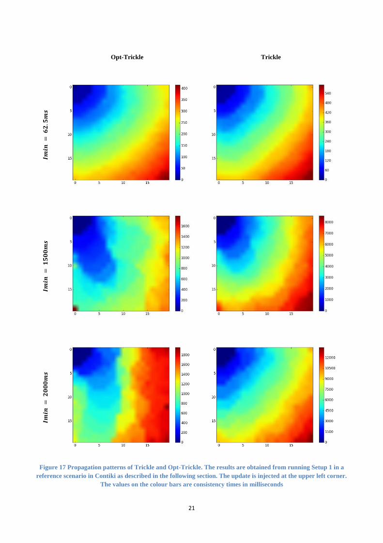
patterns for Opt-Trickle as shown in Figure 17. Thus, as can be seen from the heat maps of Figure 17, Trickle can ensure

the wavelike propagation independently from the value of 𝐼𝑚𝑖𝑛 while Opt-Trickle might have different propagation

patterns depending on the value of 𝐼𝑚𝑖𝑛. For instance, it might achieve a wavelike propagation for small values of 𝐼𝑚𝑖𝑛

under certain conditions, while realise generally free random propagation patterns. This random behaviour frees Trickle

from the wavelike propagation pattern preventing the start of the next wave until the end of the current one and hence

allows Opt-Trickle to achieve very fast propagations. Opt-Trickle’s propagation might also minimise the effect of the

dynamic behaviour of Trickle discussed in [9].

The different propagation patterns of Trickle and Opt-Trickle can have other implications on the hop count, the number

of inconsistent transmissions and other Trickle behaviours. Hence, by allowing a free random propagation, Opt-Trickle

might help the suppression mechanism and hence can generate fewer messages in the 𝐼𝑚𝑖𝑛 interval as will be observed

from in section 9. However, it is complex to exactly predict the impact and relationships between the observed propagation

patterns and Trickle behaviours (latency, number of transmissions, hop count, etc.) without a detailed thorough analysis.

Such an analysis is being prepared by the authors in order to help unveiling the ‘magic’ of Trickle’s propagation. It should

be noted that by not deploying the half-interval listen-only period in the 𝐼𝑚𝑖𝑛 interval, OS-Trickle and 𝑖Trickle(z)

propagations are essentially similar to that of Opt-Trickle. Finally, note that if the wavelike propagation ensured by a half-

interval listen-only period in the beginning of the 𝐼𝑚𝑖𝑛 interval is revealed to be a necessity, then using it with 𝑖Trickle in

the remaining intervals might present a better alternative to Trickle. In such a case, a node might start listening at time t of

an 𝐼𝑚𝑖𝑛 interval in order to minimise the number of transmissions in the following interval. This version might also be

preferred by applications deploying very small 𝐼𝑚𝑖𝑛 values such as RPL.

The remaining of this report focuses on an extensive evaluation of Opt-Trickle since it proposes the minimal changes

to Trickle which are expected to decrease dramatically its latency while preserving its cost. Preliminary results of 𝑖Trickle

along with an enhanced version are briefly discussed in section 10. Extensive evaluation and discussions of the other

proposed optimizations (𝑖Trickle(z), OS-Trickle and others) will make the subject of another report which details their

trade-offs.

S0

S1

N2

N3

N5

N4

𝑡

𝑡

𝑡

𝐼𝑚𝑖𝑛

N2

S1

N3

𝑡

𝑡

𝑡

𝐼𝑚𝑖𝑛

N2

S1

N3

The listen-only period

Implicit listen-only period Implicit listen-only period when k =1

Next wave

Current wave

21

Opt-Trickle Trickle

𝑰𝒎𝒊𝒏

= 𝟔

𝟐.𝟓

𝒎𝒔

𝑰𝒎𝒊𝒏

=

𝟏𝟓

𝟎𝟎

𝒎𝒔

𝑰𝒎𝒊𝒏

=

𝟐𝟎

𝟎𝟎

𝒎𝒔

Figure 17 Propagation patterns of Trickle and Opt-Trickle. The results are obtained from running Setup 1 in a

reference scenario in Contiki as described in the following section. The update is injected at the upper left corner.

The values on the colour bars are consistency times in milliseconds

22

8. Evaluation Methodology In this section, we outline the evaluation methodology and experimental design of this study. We conduct realistic

simulations and public testbed experiments in order to evaluate the performance of Opt-Trickle. Simulation experiments

give us controlled environments while public testbed experiments validate simulation results in real-world deployments.

To put results into context, we compared Opt-Trickle with Trickle and Short-Trickle; a version of Trickle without the

listen-only period. In what follows, we describe the implementation, the performance metrics and the experimental design.

8.1. Experimental Setup We used the Contiki OS Trickle library

6 as a basis for our modifications and evaluations. We used the default setup of

the library, which takes care of basic validity checks and adjustments, along with compensating for clock drifts. We also

implemented our modifications in TinyOS for the sake of validating the results in another environment. In both

environments, we set up two Trickle scenarios

1. Setup 1: In this setup, we generate just one inconsistent transmission, which gets propagated in the network.

Thus, a seed node in the upper-left corner of the network issues a new packet (identified by a sequence number)

once. The network uses Opt-Trickle, Trickle and Short-Trickle to propagate the packet and keep gossiping about

it until the end of the simulation time. This setup is used to get a clear understanding of Opt-Trickle.

2. Setup 2: This setup creates an abstract Trickle-based application in which a seed node periodically injects new

packets (identified by new sequence numbers) in the network. In this abstract application:

Receiving a packet with the same sequence number implies a consistency

Receiving a new packet (greater sequence number than receiver’s version) implies an inconsistency for

which the receiver updates its data and contend to propagate the update.

Receiving an old packet (smaller sequence number than receiver’s version) implies also an inconsistency

in this abstract application. In this case, the receiver shrinks its interval to 𝐼𝑚𝑖𝑛 and contends to transmit

its data in order to bring the outdated neighbour up to date.

Note that by periodically injecting new messages in the network, we deliberately create a network dominated by

inconsistent traffic in order to show the impact of the transmit-listen interplay on Opt-Trickle’s performance.

Our Trickle-based applications described in Setup 1 and Setup 2 is developed over UDP (User Datagram Protocol)

using Contiki’s micro IPv6 network stack (uIPv6) at the network layer and a CSMA-based protocol at the MAC (Media

Access Control) Layer. At the RDC (Radio Duty Cycling) layer, we opted for a non-duty cycled network. Using a non-

duty cycled network allows us to focus on Opt-Trickle’s performance rather than the effects of duty cycling. The

configurations used in all our simulations are expressed in the following points:

Nodes booted-up randomly in a 10-second period in order to avoid initially synchronised node clocks.

The CSMA/CA algorithm was configured to avoid the initial backoff7. This is so to avoid MAC randomness in

transmissions in order to get the measured times as close to determinism as possible. This configuration is

allowed by the IEEE 802.15.4’s CSMA/CA algorithm. However, there is no Collision Avoidance (CA) for the

first transmission attempt when using such a configuration. This acceptable in our case since Trickle ensures CA

by randomising transmission times. Note that while this configuration avoids delays caused by MAC backoffs,

the processing time still occur (around 20 ms in our setup). Thankfully this delay is rather deterministic. However,

it might create a situation where Trickle does not operate as expected. This is the case when a node decides to

transmit at the Trickle-layer and because of the processing time, the node receives a transmission that would

suppress its own before it is put on the air. However, Trickle cannot do anything to stop such a transmission. This

situation was observed mainly when using smaller 𝐼𝑚𝑖𝑛 values where it might affect the results. Since we opted

for a default 𝐼𝑚𝑖𝑛 = 1 𝑠𝑒𝑐𝑜𝑛𝑑, such an effect can be neglected and it does not influence the general trend.

6 https://github.com/contiki-os/contiki/blob/master/core/lib/trickle-timer.c

7 Note that this is also the default behavior of Contki’s CSMA/CA protocol

23

The MAC layer retransmissions were disabled for the sake of avoiding any interplay between MAC and Trickle

retransmissions. Under this configuration, if a Trickle transmission undergoes collisions it will be lost. Trickle

takes care of retransmissions since other nodes will transmit if they do not hear anything. In a worst case, out-

dated nodes transmissions will create inconsistencies triggering retransmission of updates. Note that disabling the

MAC layer retransmissions allows us also to measure the number of Trickle's transmissions correctly.

We used a non-duty cycled network (always on radios) in order to avoid the effects of RDC mechanisms (e.g.

delays, multiple radio transmissions…etc.) on the evaluated protocols. Note that RDC effects are being separately

examined by the authors and will be reported in a future work.

8.2. Performance Metrics In all our experiments, we focused on three main performance metrics defined below:

Transmissions/Interval: this metric is measured as the ratio between the total number of all transmissions

generated by an evaluated protocol and the number of intervals ran by the evaluated protocol during the

simulation time. Note that as Trickle Intervals have different sizes, and a protocol might have slightly less or more

intervals than another, we normalized the number of intervals across the evaluated protocols in other to provide

fair comparisons. Also, note that we sometimes (especially when using Setup 2) report the total number of

transmissions during the simulation time.

The consistency time: the consistency time is the time it takes for the whole network to be aware of an update

from its first appearance in the network. It is measured as the difference between the time when the last node gets

updated and the time when the update first appeared. It shows how fast a protocol can resolve inconsistencies.

The number of inconsistent packets: this metric measures the number of inconsistent packets generated by each

protocol, i.e. the number of transmissions in an Imin interval. As we only modify Trickle’s behaviour in an Imin-

sized interval, this metric is important to show how Opt-Trickle impacts the number of packets generated in such

an interval. In addition, it allows validating the discussion carried out in sections 4 and 5.2.

We also measured other secondary metrics in order to help explain the results, such as the number of packets generated

in the second, third and remaining intervals. Load Balancing Metric and propagation patterns are reported above.

8.3. Varied Parameters The parameters varied in this evaluation are described in the following points. In order to decide on their values, we

carried out a survey of Trickle usage in the literature with the focus on the values of 𝐼𝑚𝑖𝑛, 𝐼𝑚𝑎𝑥 and 𝑘 being deployed. In

addition to the values reported in [16], this section surveyed the recent values, not reported earlier, which are being

recommended by various IETF documents. Such values are summarised in Table 2 and discussed in the following points.

The minimum interval size: the minimum interval size Imin is varied from 62 milliseconds (ms) to 20 seconds in

order to accommodate various Trickle use-cases, ranging from those deploying very small Imin values, such as

RPL (recommended 8 ms) and CTP (default 64 ms), to those adopting large Imin values, such as in distributed

service discovery protocols. Note that while the RPL specification suggests an Imin value of 8 ms, the Contiki

RPL implementation, for instance, defaults it to 4 seconds.

The redundancy constant 𝒌: The redundancy constant k was varied between 1 and 9 for the sake of

accommodating the needs of various Trickle-based deployments such as MPL (k = 1), RPL (k = 10) or CTP

with an infinite redundancy constant (achieved through k = 0 ).

Network density: Since network density is the main factor dictating Trickle’s scalability, it was paid particular

attention in our evaluations. Thus, the number of nodes was varied between 16 and 400, thereby internetworking

up to 400 nodes simultaneously in the case of single-hop networks. In multi-hop networks, we varied the number

of nodes in a given area between 36 (allowing us to test a sparse network of an average density of 4

neighbours/node) and 196 nodes, which gives a 36 neighbours/node average density. We also fixed the number of

nodes at 400 and varied the side of the square deployment area between 300 and 400 meters, thus varying the

average density between 36 and 4 neighbours/node respectively.

24

Physical success rate: to see the impact of losses on Opt-Trickle, we varied the reception success ratio of a packet

in the cooja simulator (SUCCESS_RATIO_RX) between 10% (giving a 90% physical loss rate) and 100% (lossless

networks). We configured zero retransmissions at the MAC layer, in order to ensure that each Trickle

transmission results in exactly one MAC transmission that undergoes the reception success probability. Note that

cooja does not directly generate a uniform random probability based on the configured success ratio. Instead, it

introduces some realism to decide which node undergoes the SUCCESS_RATIO_RX based on the ratio between

reception and transmission powers. Since the Unit Disk Graph Medium (UDGM) only models attenuations as a

function of distance, and as the reception power can be proportional to the square distance between the sender and

the receiver, Cooja calculates, for each node, the 𝑅𝑒𝑐𝑒𝑝𝑡𝑖𝑜𝑛 𝑠𝑢𝑐𝑐𝑒𝑠𝑠 𝑝𝑟𝑜𝑏𝑎𝑏𝑖𝑙𝑖𝑡𝑦 as follows8:

𝑅𝑒𝑐𝑒𝑝𝑡𝑖𝑜𝑛 𝑠𝑢𝑐𝑐𝑒𝑠𝑠 𝑝𝑟𝑜𝑏𝑎𝑏𝑖𝑙𝑖𝑡𝑦 = 1.0 − 𝑟𝑎𝑡𝑖𝑜 ∗ (1.0 − 𝑆𝑈𝐶𝐶𝐸𝑆𝑆_𝑅𝐴𝑇𝐼𝑂_𝑅𝑋)

Where

𝑟𝑎𝑡𝑖𝑜 = 𝑑𝑖𝑠𝑡𝑎𝑛𝑐𝑒𝑆𝑞𝑢𝑎𝑟𝑒𝑑 / 𝑑𝑖𝑠𝑡𝑎𝑛𝑐𝑒𝑀𝑎𝑥𝑆𝑞𝑢𝑎𝑟𝑒𝑑

𝑑𝑖𝑠𝑡𝑎𝑛𝑐𝑒𝑀𝑎𝑥𝑆𝑞𝑢𝑎𝑟𝑒𝑑 is the square of the communication range, and 𝑑𝑖𝑠𝑡𝑎𝑛𝑐𝑒𝑆𝑞𝑢𝑎𝑟𝑒𝑑 represents the square

of the distance between a sender-receiver pair.

Transmission power: In testbed experiments, we varied the maximum transmission power of a sender over 5

transmission levels; namely, levels 11, 15, 18, 23 and 31, representing transmission powers at -10, -7, -5, -3 and

0 dBm respectively.

Network Topology: We used both grid and uniformly distributed topologies along with an irregular testbed

deployment. In both deployments, we evaluated sparse and dense scenarios.

Note that we also combined the above parameters. For example, we evaluated Opt-Trickle in a very lossy, dense,

uniformly deployed network with a big value of 𝑘. Finally, it should be noted that other parameters were implicitly varied

in our evaluations. For instance, the network diameter (hop count) is varied by testing 100- and 400-node networks in

similar deployments. Results from the 100-node network are depicted in Appendix C. The main evaluation parameters

used in our evaluations are summarised in Table 3.

Table 2 main Trickle parameters in the Literature

𝑰𝒎𝒊𝒏 𝑰𝒎𝒂𝒙 𝒌 𝒂𝒊𝒎

RPL-default [5] 8 ms 2.3 hours 10 quickly discover the best possible path towards

the root

P2P-RPL-default

[17]

multiple tt Large value 1 Reduce the number of messages during route

discovery

P2P-RPL-HOME

[18]

16 ms 262 s 1 Reduce network load and chances of collisions

and hidden terminals.

RPL-AMI [19] > 50 × tt 2 hours

− 2 days

> 10 Quickly discover the best path towards the root

and reduce chances of collisions and hidden

terminals.

ContikiRPL9 4𝑠 1048 s 10 Account for RDC and MAC delays

MPL-default

(proactive) [7]

10 × tt Imax = Imin 1 Reduce chances of collisions and hidden

terminals.

MPL-default

(reactive) [7]

10 × tt 300 seconds 1 Reduce chances of collisions and hidden

terminals.

MPL-HOME

(proactive) [18]

10 – 50 ms 100 − 400 ms 2 − 3 Achieve 200 ms deadline over 5 hops

CTP [6] 64 ms 1 hour ∞ (0) quickly discover the best possible path towards

the root

8 https://github.com/contiki-os/contiki/blob/master/tools/cooja/java/org/contikios/cooja/radiomediums/UDGM.java

9 https://github.com/contiki-os/contiki/blob/master/core/net/rpl/rpl-conf.h

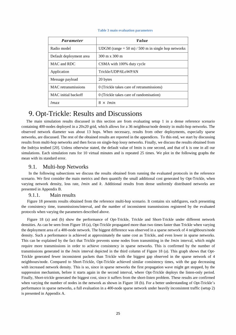
25

Table 3 main evaluation parameters

𝑷𝒂𝒓𝒂𝒎𝒆𝒕𝒆𝒓 𝑽𝒂𝒍𝒖𝒆

Radio model UDGM (range = 50 m) / 500 m in single hop networks

Default deployment area 300 m x 300 m

MAC and RDC CSMA with 100% duty cycle

Application Trickle/UDP/6LoWPAN

Message payload 20 bytes

MAC retransmissions 0 (Trickle takes care of retransmissions)

MAC initial backoff 0 (Trickle takes care of randomisation)

𝐼𝑚𝑎𝑥 8 × 𝐼𝑚𝑖𝑛

9. Opt-Trickle: Results and Discussions The main simulation results discussed in this section are from evaluating setup 1 in a dense reference scenario

containing 400-nodes deployed in a 20x20 grid, which allows for a 36 neighbour/node density in multi-hop networks. The

observed network diameter was about 13 hops. When necessary, results from other deployments, especially sparse

networks, are discussed. The rest of the obtained results are reported in the appendices. To this end, we start by discussing

results from multi-hop networks and then focus on single-hop lossy networks. Finally, we discuss the results obtained from

the Indriya testbed [20]. Unless otherwise stated, the default value of Imin is one second, and that of k is one in all our

simulations. Each simulation runs for 10 virtual minutes and is repeated 25 times. We plot in the following graphs the

mean with its standard error.

9.1. Multi-hop Networks In the following subsections we discuss the results obtained from running the evaluated protocols in the reference

scenario. We first consider the main metrics and then quantify the small additional cost generated by Opt-Trickle, when

varying network density, loss rate, 𝐼𝑚𝑖𝑛 and 𝑘. Additional results from dense uniformly distributed networks are

presented in Appendix B.

9.1.1. Main results Figure 18 presents results obtained from the reference multi-hop scenario. It contains six subfigures, each presenting

the consistency time, transmissions/interval, and the number of inconsistent transmissions registered by the evaluated

protocols when varying the parameters described above.

Figure 18 (a) and (b) show the performance of Opt-Trickle, Trickle and Short-Trickle under different network

densities. As can be seen from Figure 18 (a), Opt-Trickle propagated more than two times faster than Trickle when varying

the deployment area of a 400-node network. The biggest difference was observed in a sparse network of 4 neighbours/node

density. Such a performance is achieved at approximately the same cost as Trickle, and even lower in sparse networks.

This can be explained by the fact that Trickle prevents some nodes from transmitting in the 𝐼𝑚𝑖𝑛 interval, which might

require more transmissions in order to achieve consistency in sparse networks. This is confirmed by the number of

transmissions generated in the 𝐼𝑚𝑖𝑛 interval depicted in the third column of Figure 18 (a). This graph shows that Opt-

Trickle generated fewer inconsistent packets than Trickle with the biggest gap observed in the sparse network of 4

neighbours/node. Compared to Short-Trickle, Opt-Trickle achieved similar consistency times, with the gap decreasing

with increased network density. This is so, since in sparse networks the first propagation wave might get stopped, by the

suppression mechanism, before it starts again in the second interval, where Opt-Trickle deploys the listen-only period.

Finally, Short-trickle generated the biggest cost, since it suffers from the short-listen problem. These results are confirmed

when varying the number of nodes in the network as shown in Figure 18 (b). For a better understanding of Opt-Trickle’s

performance in sparse networks, a full evaluation in a 400-node sparse network under heavily inconsistent traffic (setup 2)

is presented in Appendix A.

26

Concerning the impact of losses, Figure 18 (c) presents the performance of Opt-Trickle, Trickle and Short-Trickle

when varying the physical loss rate. As can be seen from this figure, Opt-Trickle approached the propagation time of

Short-Trickle even in a worst case of 90% loss rate. The gap between the two protocols decreased with increasing success

rates. This is explained by the fact that in very lossy networks there are more chances of losing an update for the first time

which postpones its delivery until the next interval. In such an interval, Opt-Trickle deploys the listen-only period, while

Short-Trickle does not, allowing it to propagate faster. In all cases, the consistency time of both Short-Trickle and Opt-

Trickle was about four times lower than that of Trickle. While Short-Trickle achieved such a performance by generating

more packets, Opt-Trickle generated approximately the same cost as Trickle. Upon a closer look, Opt-Trickle generated

slightly more packets than Trickle which are more visible in lossy networks. This is explained by the transmit-listen

interplay benefiting Trickle, which is quantified in the following subsection. However, the packets generated by Opt-

Trickle in the 𝐼𝑚𝑖𝑛 interval are still fewer than that of Trickle.

Figure 18 (d) depicts the performance of Opt-Trickle when varying 𝐼𝑚𝑖𝑛 in a physically lossless network. As expected,

Opt-Trickle achieved network consistency as quickly as Short-Trickle. Interestingly, the propagation time of Opt-Trickle

does not heavily depend on 𝐼𝑚𝑖𝑛 as is the case for Trickle, thereby allowing Opt-Trickle to propagate new updates seven

times faster in an 𝐼𝑚𝑖𝑛 of two seconds. This gap is expected to increase with increased 𝐼𝑚𝑖𝑛 values. While short-Trickle

achieved such a propagation speed generating more messages, the cost of Opt-Trickle is similar to that of Trickle. It should

be noted, however, that a small difference in the cost of the two protocols can be observed, and it is more visible for

smaller 𝐼𝑚𝑖𝑛 values. This can be due to two main reasons; namely, losses and unbalanced load distribution, both

benefiting Trickle in dense networks. Thus, even though the network is physically lossless, losses can always occur

because of collisions and hidden terminals, which are more likely to occur in small contending periods i.e. smaller 𝐼𝑚𝑖𝑛

intervals. On the other hand, since Trickle explicitly prevents some nodes from transmitting, it minimises the number of

contenders in an 𝐼𝑚𝑖𝑛 interval, which in turn minimises losses. This is confirmed from the inconsistent transmissions

graph, which shows that Opt-Trickle generated about 60% more transmissions in an 𝐼𝑚𝑖𝑛 interval of 62 ms. This gap

decreased dramatically, such that in an 𝐼𝑚𝑖𝑛 of 125 ms, Opt-Trickle only added about 20% extra packets, and from an

𝐼𝑚𝑖𝑛 of one second, Opt-Trickle generated less overhead than Trickle. This might be caused by the propagation patterns

discussed in section 7. Note that this only benefits Trickle in dense networks, while it constitutes a drawback for Trickle in

sparse networks, as shown in Appendix A. Thus, in sparse networks, Opt-Trickle outperformed Trickle in both time/cost

aspects when varying 𝐼𝑚𝑖𝑛 using the default value of 𝑘 = 1.

Finally, Figure 18 (e) and (f) present the performance of the evaluated algorithms when varying the redundancy

constant in both physically lossless and very lossy networks. As can be seen from these figures, increasing 𝑘 decreased

slightly the network consistency time while increased considerably the cost of the three protocols in both lossy and lossless

dense networks. This observation remains valid in sparse networks, as can be seen from Appendix A. Concerning

individual protocols performance, Figure 18 (e) shows that Opt-Trickle propagated about 3.5 times faster than Trickle

while also generating fewer messages when increasing 𝑘. This can be explained by the fact that in physically lossless

dense networks, Opt-Trickle suffers less from the transmit-listen interplay, while at the same time benefiting from fewer

transmissions in an 𝐼𝑚𝑖𝑛 interval. This is confirmed from the graph of generated inconsistent packets, which shows that

the additional cost of Trickle increased with increasing 𝑘 values. However, this is not the case in sparse networks

experiencing heavily inconsistent traffic. Thus, in such a configuration, Opt-Trickle generated slightly more transmissions

than Trickle when 𝑘 increased, as shown in Appendix A. This can be due to the transmit-listen interplay helping Trickle’s

consistency counter to reach 𝑘 without actually generating 𝑘 packets. When taking link drops into consideration, Figure 18

(f) shows that Opt-Trickle can compensate for the additional cost caused from lacking the transmit-listen interplay by

using the transmissions saved in the 𝐼𝑚𝑖𝑛 Interval.

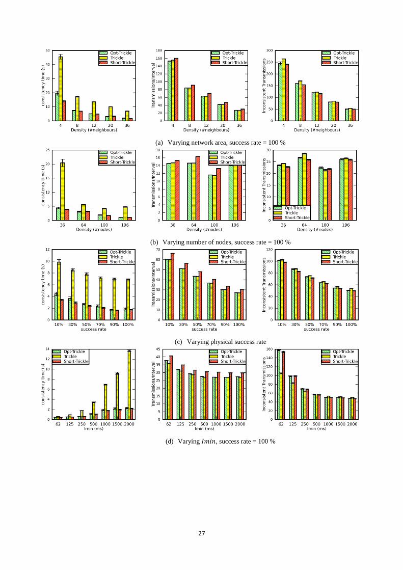
27

(a) Varying network area, success rate = 100 %

(b) Varying number of nodes, success rate = 100 %

(c) Varying physical success rate

(d) Varying 𝐼𝑚𝑖𝑛, success rate = 100 %

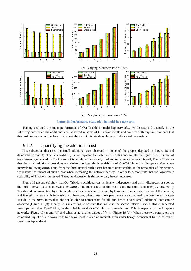
28

(e) Varying 𝑘, success rate = 100%

(f) Varying 𝑘, success rate = 10%

Figure 18 Performance evaluation in multi-hop networks

Having analysed the main performance of Opt-Trickle in multi-hop networks, we discuss and quantify in the

following subsection the additional cost observed in some of the above results and confirm with experimental data that

this cost does not affect the logarithmic scalability of Opt-Trickle under any of the varied parameters.

9.1.2. Quantifying the additional cost This subsection discusses the small additional cost observed in some of the graphs depicted in Figure 18 and

demonstrates that Opt-Trickle’s scalability is not impacted by such a cost. To this end, we plot in Figure 19 the number of

transmissions generated by Trickle and Opt-Trickle in the second, third and remaining intervals. Overall, Figure 19 shows

that the small additional cost does not violate the logarithmic scalability of Opt-Trickle and it disappears after a few

intervals following 𝐼𝑚𝑖𝑛. Thus, from the third interval such a cost becomes unnoticeable. In the remainder of this section,

we discuss the impact of such a cost when increasing the network density, in order to demonstrate that the logarithmic

scalability of Trickle is preserved. Then, the discussion is shifted to only interesting cases.

Figure 19 (a) and (b) show that Opt-Trickle’s additional cost is density independent and that it disappears as soon as

the third interval (second interval after 𝐼𝑚𝑖𝑛). The main cause of this cost is the transmit-listen interplay ensured by

Trickle and not guaranteed by Opt-Trickle. Such a cost is mainly caused by losses and the multi-hop nature of the network,

and it might increase with increasing 𝑘. Therefore, when these three parameters are combined, the cost saved by Opt-

Trickle in the 𝐼𝑚𝑖𝑛 interval might not be able to compensate for all, and hence a very small additional cost can be

observed (Figure 19 (f)). Finally, it is interesting to observe that, while in the second interval Trickle always generated

fewer packets than Opt-Trickle, in the third interval Opt-Trickle can transmit less. This is especially true in sparse

networks (Figure 19 (a) and (b)) and when using smaller values of 𝐼𝑚𝑖𝑛 (Figure 19 (d)). When these two parameters are

combined, Opt-Trickle always leads to a fewer cost in such an interval, even under heavy inconsistent traffic, as can be

seen from Appendix A.

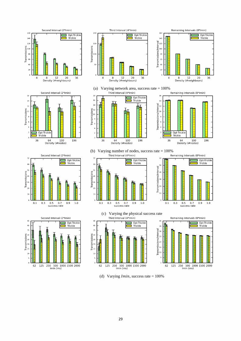
29

(a) Varying network area, success rate = 100%

(b) Varying number of nodes, success rate = 100%

(c) Varying the physical success rate

(d) Varying 𝐼𝑚𝑖𝑛, success rate = 100%

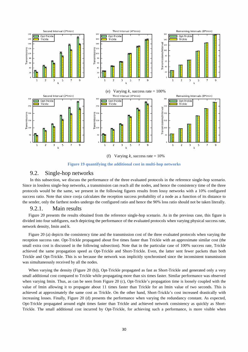
30

(e) Varying 𝑘, success rate = 100%

(f) Varying 𝑘, success rate = 10%

Figure 19 quantifying the additional cost in multi-hop networks

9.2. Single-hop networks In this subsection, we discuss the performance of the three evaluated protocols in the reference single-hop scenario.

Since in lossless single-hop networks, a transmission can reach all the nodes, and hence the consistency time of the three

protocols would be the same, we present in the following figures results from lossy networks with a 10% configured

success ratio. Note that since cooja calculates the reception success probability of a node as a function of its distance to

the sender, only the farthest nodes undergo the configured ratio and hence the 90% loss ratio should not be taken literally.

9.2.1. Main results Figure 20 presents the results obtained from the reference single-hop scenario. As in the previous case, this figure is

divided into four subfigures, each depicting the performance of the evaluated protocols when varying physical success rate,

network density, Imin and k.

Figure 20 (a) depicts the consistency time and the transmission cost of the three evaluated protocols when varying the

reception success rate. Opt-Trickle propagated about five times faster than Trickle with an approximate similar cost (the

small extra cost is discussed in the following subsection). Note that in the particular case of 100% success rate, Trickle

achieved the same propagation speed as Opt-Trickle and Short-Trickle. Even, the latter sent fewer packets than both

Trickle and Opt-Trickle. This is so because the network was implicitly synchronised since the inconsistent transmission

was simultaneously received by all the nodes.

When varying the density (Figure 20 (b)), Opt-Trickle propagated as fast as Short-Trickle and generated only a very

small additional cost compared to Trickle while propagating more than six times faster. Similar performance was observed

when varying Imin. Thus, as can be seen from Figure 20 (c), Opt-Trickle’s propagation time is loosely coupled with the

value of Imin allowing it to propagate about 11 times faster than Trickle for an Imin value of two seconds. This is

achieved at approximately the same cost as Trickle. On the other hand, Short-Trickle’s cost increased drastically with

increasing losses. Finally, Figure 20 (d) presents the performance when varying the redundancy constant. As expected,

Opt-Trickle propagated around eight times faster than Trickle and achieved network consistency as quickly as Short-

Trickle. The small additional cost incurred by Opt-Trickle, for achieving such a performance, is more visible when

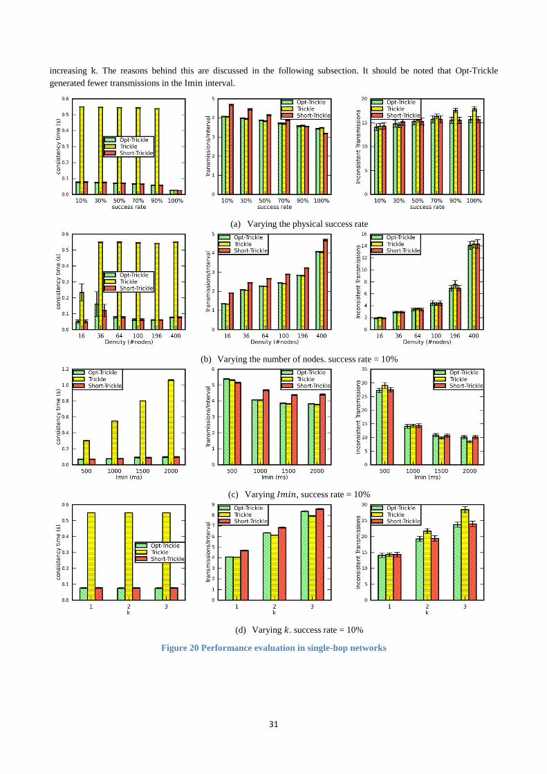
31

increasing k. The reasons behind this are discussed in the following subsection. It should be noted that Opt-Trickle

generated fewer transmissions in the Imin interval.

(a) Varying the physical success rate

(b) Varying the number of nodes. success rate = 10%

(c) Varying 𝐼𝑚𝑖𝑛, success rate = 10%

(d) Varying 𝑘. success rate = 10%

Figure 20 Performance evaluation in single-hop networks

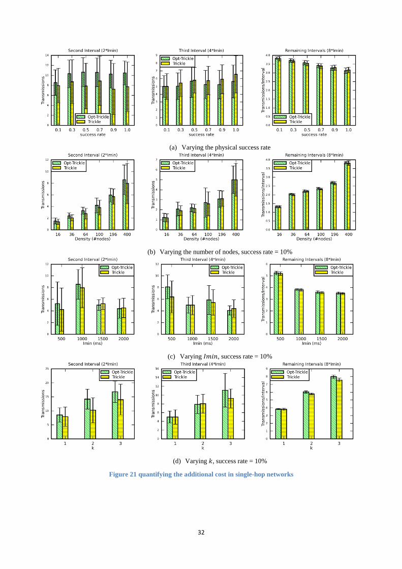
32

(a) Varying the physical success rate

(b) Varying the number of nodes, success rate = 10%

(c) Varying 𝐼𝑚𝑖𝑛, success rate = 10%

(d) Varying 𝑘, success rate = 10%

Figure 21 quantifying the additional cost in single-hop networks

33

9.2.2. Quantifying the additional cost As in multi-hop networks, we discuss in this subsection the additional cost generated by Opt-Trickle in single-hop

networks and show that it does not impact Opt-Trickle’s logarithmic scalability.

Figure 21 quantifies the additional cost introduced by Opt-Trickle in the second, third and remaining intervals.

Similarly to multi-hop networks, this additional cost does not depend on the number of nodes in the network, as can be

seen from Figure 21 (b), and it can disappear after the third interval when using a default value of k = 1. Similar trends

were also observed when varying the physical success ratio (Figure 21 (a)) and Imin (Figure 21 (c)).

When 𝑘 increased however, the additional cost generated by Opt-Trickle was still observable even in the remaining

intervals. This can be explained by the transmit-listen interplay benefiting Trickle in a network of 400 internetworked

direct neighbours. Thus, combining a very dense single-hop network, suffering severe losses and using increased 𝑘 values

allowed such an additional cost to be made more visible. Nevertheless, and even in this very constrained scenario, the

additional cost generated by Opt-Trickle remains independent from the network density and therefore does affect Opt-

Trickle’s scalability.

9.3. Empirical Study As mentioned earlier, Opt-Trickle was also evaluated in the public large-scale Indriya testbed [20]. Indriya contains

around 100 active motes irregularly deployed in a three floor building at the national university of Singapore. The layout of

the Indriya testbed is presented in Appendix E. At the time of experimentation almost all middle floor nodes were off,

leaving us with 65 motes and a good opportunity to test in an irregular, faulty real-world scenario. Using setup 2, the seed

(node 21 in the third floor) injected a new packet every 60 seconds. This is so to create a network dominated by

inconsistent traffic, in order to show the impact of the observed small additional cost in the simulation results. Each

experiment was run for 30 minutes and was repeated three times. The default value of 𝐼𝑚𝑖𝑛 was half a second and that of

𝑘 was one. As in the simulations, we report in the graphs the mean along with its standard error.

9.3.1. Main results Figure 22 presents the consistency time, the total transmissions and the number of inconsistent packets registered by

Opt-Trickle, Trickle and Short-Trickle when varying the minimum interval size, the redundancy constant and node

transmission power.

Figure 22 (a) depicts Opt-Trickle’s performance when varying 𝐼𝑚𝑖𝑛. As can be seen from these graphs, Opt-Trickle

achieved network consistency faster than Trickle, while approximately generating a similar number of transmissions. The

small additional cost is due to the transmit-listen interplay discussed earlier. Note that even in this very irregular faulty

network Opt-Trickle’s propagation speed is less affected by the value of 𝐼𝑚𝑖𝑛. Concerning the number of generated

inconsistent transmissions and similarly to previous results, Opt-Trickle generated fewer packets in the 𝐼𝑚𝑖𝑛 interval when

the interval size was greater than 125 𝑚𝑠. In an 𝐼𝑚𝑖𝑛 = 62 𝑚𝑠, Trickle transmitted fewer packets, since it explicitly

prevented some nodes form contending and hence minimised the chances for collisions and hidden terminals.

When varying 𝑘, as can be observed from Figure 22 (b), Opt-Trickle provided the best of both Trickle and Short-

Trickle, even in this faulty irregular network experiencing heavy inconsistent traffic. Thus, it propagated new updates as

quickly as Short-Trickle, which is about twice faster than Trickle, at a similar transmission cost. When considering the

number of transmissions in the 𝐼𝑚𝑖𝑛 interval, Opt-Trickle generated less overhead than Trickle.

Finally, the third row of graphs depicted in Figure 22 (c) shows the performance of the evaluated protocols when

varying transmission power. Varying transmission power plays a double role; it changes both the density and the success

rate of the network. As can be seen from Figure 22 (c), Opt-Trickle propagated about twice faster than Trickle, even in a

quite lossy, less connected network (power level 11 at -10 dBm). As expected and for the reasons disused earlier, Opt-

Trickle’s consistency time approached that of Short-Trickle, with a cost similar to that of Trickle.

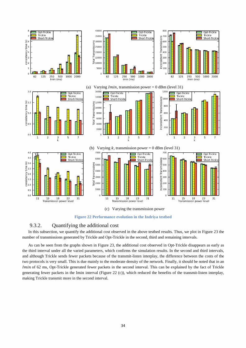
34

(a) Varying 𝐼𝑚𝑖𝑛, transmission power = 0 dBm (level 31)

(b) Varying 𝑘, transmission power = 0 dBm (level 31)

(c) Varying the transmission power

Figure 22 Performance evolution in the Indriya testbed

9.3.2. Quantifying the additional cost In this subsection, we quantify the additional cost observed in the above testbed results. Thus, we plot in Figure 23 the

number of transmissions generated by Trickle and Opt-Trickle in the second, third and remaining intervals.

As can be seen from the graphs shown in Figure 23, the additional cost observed in Opt-Trickle disappears as early as

the third interval under all the varied parameters, which confirms the simulation results. In the second and third intervals,

and although Trickle sends fewer packets because of the transmit-listen interplay, the difference between the costs of the

two protocols is very small. This is due mainly to the moderate density of the network. Finally, it should be noted that in an

𝐼𝑚𝑖𝑛 of 62 ms, Opt-Trickle generated fewer packets in the second interval. This can be explained by the fact of Trickle

generating fewer packets in the Imin interval (Figure 22 (c)), which reduced the benefits of the transmit-listen interplay,

making Trickle transmit more in the second interval.

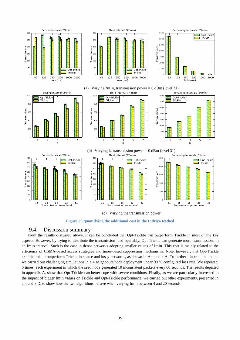
35

(a) Varying 𝐼𝑚𝑖𝑛, transmission power = 0 dBm (level 31)

(b) Varying k, transmission power = 0 dBm (level 31)

(c) Varying the transmission power

Figure 23 quantifying the additional cost in the Indriya testbed

9.4. Discussion summary From the results discussed above, it can be concluded that Opt-Trickle can outperform Trickle in most of the key

aspects. However, by trying to distribute the transmission load equitably, Opt-Trickle can generate more transmissions in

an Imin interval. Such is the case in dense networks adopting smaller values of Imin. This cost is mainly related to the

efficiency of CSMA-based access strategies and timer-based suppression mechanisms. Note, however, that Opt-Trickle

exploits this to outperform Trickle in sparse and lossy networks, as shown in Appendix A. To further illustrate this point,

we carried out challenging simulations in a 4 neighbours/node deployment under 90 % configured loss rate. We repeated,

5 times, each experiment in which the seed node generated 10 inconsistent packets every 60 seconds. The results depicted

in appendix A, show that Opt-Trickle can better cope with severe conditions. Finally, as we are particularly interested in

the impact of bigger Imin values on Trickle and Opt-Trickle performance, we carried out other experiments, presented in

appendix D, to show how the two algorithms behave when varying Imin between 4 and 20 seconds.

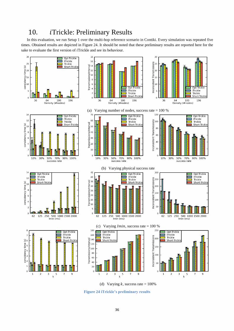
36

10. 𝑖Trickle: Preliminary Results In this evaluation, we run Setup 1 over the multi-hop reference scenario in Contiki. Every simulation was repeated five

times. Obtained results are depicted in Figure 24. It should be noted that these preliminary results are reported here for the

sake to evaluate the first version of 𝑖Trickle and see its behaviour.

(a) Varying number of nodes, success rate = 100 %

(b) Varying physical success rate

(c) Varying 𝐼𝑚𝑖𝑛, success rate = 100 %

(d) Varying 𝑘, success rate = 100%

Figure 24 iTrickle’s preliminary results

37

Overall 𝑖Trickle outperforms all the evaluated protocols concerning the latency under all varied parameters. This is

especially observable in lossy networks (Figure 24 (b)). However, these preliminary results show that the cost generated by

𝑖Trickle varies depending on the density (Figure 24 (a)). Thus, it generates slightly more than Trickle and Opt-Trickle in

sparse networks and generates less when the density increases. Thus, for dense networks and under all the varied

parameters, 𝑖Trickle generated the smallest number of messages in conformance with the discussion carried out in section

6.2. Concerning the number of generated messages in the Imin interval, iTrickle seems to generate the biggest number.

This is especially observed with smaller Imin intervals and it is the result of halving the size of the Imin interval without

the ‘magic’ discussed in section 7. This observation suggests substituting the behaviour of 𝑖Trickle in the Imin interval by

the one of Opt-Trickle, which showed to be less affected by this problem. This should be done while allowing nodes to

listen at time t of the Imin interval. With this modification, 𝑖Trickle is described as follows:

This version of 𝑖Trickle is under extensive evaluations which show good performance. It performs similarly to the

evaluated version of 𝑖Trickle in terms of latency and smaller general cost, and to Opt-Trickle in terms of the cost in the

𝐼𝑚𝑖𝑛 interval.

11. Expected Impact Since 𝑖Trickle is still work in progress, this section only discusses the expected impact of Opt-Trickle. Overall, all

Trickle-based applications can benefit from Opt-Trickle by modifying only a single line of code. Here we focus on the

IETF standards RPL [5] and MPL [7].

RPL relies on Trickle for controlling the frequency of DIO (DODAG Information Object) messages, which constitute

the basic building block of the DODAG (Destination Oriented Directed Acyclic Graph). Therefore, Trickle plays an

important role in the convergence time and stability of RPL networks. In order to maintain a low consistency time, 𝐼𝑚𝑖𝑛 is

recommended to equal 8 ms and 𝑘 is conservatively proposed to equal 10. Opt-Trickle can offer faster consistency times

even when using small Imin values, which helps to speed-up RPL’s convergence. More importantly as Opt-Trickle

propagation is loosely coupled with the value of Imin, choosing a big value of Imin can still allow a low RPL convergence

time while minimizing the generated cost. In addition, as RPL uses big 𝑘 values, the small additional cost observed in Opt-

Trickle for equitably distributing the load can be compensated by the benefit of lower cost in the 𝐼𝑚𝑖𝑛 interval. Finally,

Opt-Trickle may also prompt a new discussion of RPL’s Trickle parameters and allow for a smaller value of 𝑘 in order to

minimize the cost of building and maintaining the DODAG.

On the other hand, MPL uses Trickle in both its proactive and reactive modes in order to achieve reliable multicast

forwarding in LLNs. Opt-Trickle allows MPL to deliver multicast packets much faster. For instance, MPL’s proactive

mode recommends a default configuration of 𝑘 = 1 and 𝐼𝑚𝑎𝑥 = 𝐼𝑚𝑖𝑛, which invites most of the criticisms discussed in

section 2.2, especially those concerning load distribution. Therefore, Opt-Trickle allows MPL’s proactive mode to provide

a balanced load distribution and, more importantly, avoids preventing some nodes from transmitting. It should be noted

that MPL’s proactive mode prevents this issue from becoming infinite by stopping a Trickle data timer after a specific

number of expirations, recommended to equal 3. In addition, the optional proactive mode is backed by the reactive mode.

Finally, Opt-Trickle can help MPL’s reactive mode to achieve a better load distribution and a faster inconsistency

resolution time.

Finally, by providing fast propagation times which are loosely-coupled to the value of 𝐼𝑚𝑖𝑛, Opt-Trickle can open

doors for new soft real-time use cases of the Trickle algorithm.

𝑺𝒕𝒆𝒑 𝟐: When an interval begins, 𝑖Trickle picks 𝑡 uniformly at random from the range:

- [0; 𝐼𝑚𝑖𝑛), if the interval began as a result of 𝑺𝒕𝒆𝒑 𝟔 (because of an inconsistency or in response to

external events). 𝑖Trickle then resets c to 0.

- [0, 𝐼/2), otherwise (the interval began as a result of 𝑺𝒕𝒆𝒑 𝟏 or 𝑺𝒕𝒆𝒑 𝟓).

𝑺𝒕𝒆𝒑 𝟒: At time t of the current interval I, iTrickle transmits if and only if c is less than k. Otherwise, the

transmission is suppressed. 𝑖Trickle then resets c to 0.

iTrickle

38

12. Related Work We discuss in this section related works trying to alter Trickle’s behaviour. These works can be divided into two

categories: those trying to tweak Trickle’s behaviour in specific use-cases, such as in RPL and MPL, and those studying

Trickle’s behaviour in the generic case, similar to our study.

As described earlier, RPL deploys Trickle to schedule DIO transmissions and, hence, dictates the consistency of the

DODAG over time. This motivated researchers to study Trickle in order to predict the performance of RPL networks. For

instance, [21] tries to make Trickle fair to all RPL nodes. Thus, it proposes to bias the uniform choice of transmission

times by giving the nodes that sent fewer packets in the past more chances to transmit in the future. The authors of [22]

study the effect of non-synchronised Trickle intervals on RPL’s generated control traffic. To tackle this effect, the authors

proposed a readjustment of trickle intervals in order to gradually re-establish synchronisation. The authors claim that the

proposed scheme could fall back to Trickle in a worst case.

MPL describes a way of using Trickle to realise reliable multicast routing in LLNs. To this end, MPL introduces a

fourth Trickle parameter, which allows stopping a Trickle timer after a specific number of expirations. This allows

efficient usage of the limited resources on constrained nodes especially since MPL’s proactive mode requires for a node to

create and manage a Trickle timer per packet. Also note that MPL uses Trickle to manage multiple data items in both

proactive and reactive modes. Thus, it deploys, for the proactive mode, parallel Trickle approaches similar to the ones

applied in [11][23]. For the reactive mode, MPL uses serial Trickle approaches [24].

Other works focusing on analytically modelling Trickle’s behaviour in order to predict its performance in generic cases

are reported in [25][26][27]. These works try to provide mathematical tools that can analytically predict the message count

and the propagation of Trickle. For instance, a detailed analytical study of Trickle’s behaviour is reported in [27] where the

message count and propagation time are analytically modelled as a function of a generalised listen-only period. In a recent

work [28] published in parallel to our previous work [29], the authors moved the parametric listen-only period to the 𝐼𝑚𝑖𝑛

interval. Although, the theoretical modelling presented in [28] only treats lossless line-topology networks, the results

confirm our experimental findings discussed in [29]. Generally speaking, while these models can help understand Trickle

dynamics, they assume simplistic, lossless and regular network deployments. In addition, such models neither consider

realistic radio propagation patterns nor model contentions and collisions, which is an oversimplification of LLN dynamics.

13. Conclusion In this report, we introduced, discussed and evaluated Opt-Trickle, OS-Trickle and 𝑖Trickle(z). Extensive results of

Opt-Trickle showed important performance improvements over Trickle, especially in the consistency time, while at the

same time preserving Trickle’s scalability. Preliminary results of 𝑖Trickle, OS-Trickle and Opt-Trickle variants are also

very promising. Nevertheless, many enhancements can be added to the proposed optimisations. For instance, all the

optimisations work on the assumption that an inconsistent transmission is received simultaneously by all receivers. While,

this assumption seems reasonable in many cases, it can be challenged by some RDC protocols which change the semantics

of broadcasts, such as ContikiMAC [30]. In addition, transmission and reception energy profiles are entirely different in

duty-cycled networks, with a transmission costing over 10 times the cost of a reception [31]. This makes the

communication load more costly for senders than for receivers, and hence asks for a better transmission load balancing.

Moreover, detailed analysis, discussions and modelling of the proposed optimisations are required in order to get a better

understanding of their behaviours. The first issue regarding duty-cycling was recently addressed in [32]. The two others

are being currently addressed by the authors. Other optimizations are also being investigated along with analytical

modelling in order to draw conclusions when to use Trickle, Opt-Trickle, OS-Trickle and/or 𝑖Trickle. Such an analysis

aims to propose a general version of Trickle that expands its usage even further.

Finally, it should be noted that although we have provided some experimental evidence under Contiki OS and TinyOS,

more evaluations, discussions and analysis are required to fully understand the behaviours of the proposed optimizations

and demonstrate they do not violate Trickle assumptions in the most severe conditions.

Acknowledgments

The authors would like to acknowledge early discussions with Philip Levis that helped to shape this report.

39

References

[1] “10 Emerging Technologies That Will Change the World - MIT Technology Review.” [Online]. Available: http://www2.technologyreview.com/featured-story/401775/10-emerging-technologies-that-will-change-the/3/. [Accessed: 20-Nov-2013].

[2] L. Atzori, A. Iera, and G. Morabito, “The Internet of Things: A survey,” Comput. Netw., vol. 54, no. 15, pp. 2787–2805, Oct. 2010.

[3] P. Levis, N. Patel, D. Culler, and S. Shenker, “Trickle: A Self-Regulating Algorithm for Code Propagation and Maintenance in Wireless Sensor Networks,” in In Proceedings of the First USENIX/ACM Symposium on Networked Systems Design and Implementation (NSDI, 2004, pp. 15–28.

[4] P. Levis, T. Clausen, J. Hui, O. Gnawali, and J. Ko, “RFC 6206: The trickle algorithm,” IETF, 2011. [5] T. Winter, P. Thubert, A. Brandt, J. Hui, R. Kelsey, P. Levis, K. Pister, R. Struik, J. P. Vasseur, and R. Alexander, “RFC

6550: RPL: IPv6 Routing Protocol for Low-Power and Lossy Networks,” Mar. 2012. [6] O. Gnawali, R. Fonseca, K. Jamieson, D. Moss, and P. Levis, “Collection tree protocol,” in Proceedings of the 7th

ACM Conference on Embedded Networked Sensor Systems, 2009, pp. 1–14. [7] J. Hui and R. Kelsey, “Multicast Protocol for Low power and Lossy Networks (MPL),” 2014. [8] B. Djamaa, M. Richardson, N. Aouf, and B. Walters, “Towards efficient distributed service discovery in low-power

and lossy networks,” Wirel. Netw., vol. 20, no. 8, pp. 2437–2453, Nov. 2014. [9] A. Chlipala, J. Hui, and G. Tolle, “Deluge: data dissemination for network reprogramming at scale,” Univ. Calif.

Berkeley Tech Rep, 2004. [10] K. Lin and P. Levis, “Data discovery and dissemination with dip,” in Proceedings of the 7th international

conference on Information processing in sensor networks, 2008, pp. 433–444. [11] G. Tolle and D. Culler, “Design of an application-cooperative management system for wireless sensor networks,”

in Wireless Sensor Networks, 2005. Proceeedings of the Second European Workshop on, 2005, pp. 121–132. [12] T. Dang, N. Bulusu, W.-C. Feng, and S. Park, “Dhv: A code consistency maintenance protocol for multi-hop

wireless sensor networks,” in Wireless Sensor Networks, Springer, 2009, pp. 327–342. [13] P. Levis, E. Brewer, D. Culler, D. Gay, S. Madden, N. Patel, J. Polastre, S. Shenker, R. Szewczyk, and A. Woo, “The

emergence of a networking primitive in wireless sensor networks,” Commun. ACM, vol. 51, no. 7, pp. 99–106, 2008.

[14] IEEE Computer Society, LAN/MAN Standards Committee, Institute of Electrical and Electronics Engineers, and IEEE-SA Standards Board, IEEE standard for information technology telecommunications and information exchange between systems--local and metropolitan area networks--specific requirements. Part 15.4, Part 15.4,. New York, NY: Institute of Electrical and Electronics Engineers, 2006.

[15] H. Lee, A. Cerpa, and P. Levis, “Improving wireless simulation through noise modeling,” in Information Processing in Sensor Networks, 2007. IPSN 2007. 6th International Symposium on, 2007, pp. 21–30.

[16] A. Filippoupolitis, L. Hey, G. Loukas, E. Gelenbe, and S. Timotheou, “Emergency response simulation using wireless sensor networks,” in Proceedings of the 1st international conference on Ambient media and systems, 2008, p. 21.

[17] M. Goyal, E. Baccelli, M. Philipp, A. Brandt, and J. Martocci, “RFC 6997: Reactive Discovery of Point-to-Point Routes in Low Power and Lossy Networks,” Aug. 2013.

[18] A. Brandt, E. Baccelli, R. Cragie, and P. V. der Stok, “Applicability Statement: The use of the RPL protocol suite in Home Automation and Building Control.” [Online]. Available: http://tools.ietf.org/html/draft-ietf-roll-applicability-home-building-07. [Accessed: 17-Feb-2015].

[19] D. Popa, M. Gillmore, L. Toutain, J. Hui, r Ruben, K. Monden, and N. Cam-Winget, “Applicability Statement for the Routing Protocol for Low Power and Lossy Networks (RPL) in AMI Networks.” [Online]. Available: http://tools.ietf.org/html/draft-ietf-roll-applicability-ami-10. [Accessed: 17-Feb-2015].

[20] M. Doddavenkatappa, M. C. Chan, and A. L. Ananda, “Indriya: A low-cost, 3D wireless sensor network testbed,” in Testbeds and Research Infrastructure. Development of Networks and Communities, Springer, 2012, pp. 302–316.

[21] C. Vallati and E. Mingozzi, “Trickle-F: Fair broadcast suppression to improve energy-efficient route formation with the RPL routing protocol,” in Sustainable Internet and ICT for Sustainability (SustainIT), 2013, 2013, pp. 1–9.

[22] J. Eriksson and O. Gnawali, “Synchronizing Trickle Intervals.” [23] J. W. Hui and D. Culler, “The dynamic behaviour of a data dissemination protocol for network programming at

scale,” in Proceedings of the 2nd international conference on Embedded networked sensor systems, 2004, pp. 81–94.

40

[24] O. Gnawali, K.-Y. Jang, J. Paek, M. Vieira, R. Govindan, B. Greenstein, A. Joki, D. Estrin, and E. Kohler, “The tenet architecture for tiered sensor networks,” in Proceedings of the 4th international conference on Embedded networked sensor systems, 2006, pp. 153–166.

[25] H. Kermajani, C. Gomez, and M. H. Arshad, “Modeling the Message Count of the Trickle Algorithm in a Steady-State, Static Wireless Sensor Network,” IEEE Commun. Lett., vol. 16, no. 12, pp. 1960–1963, Dec. 2012.

[26] M. Becker, K. Kuladinithi, and C. Görg, “Modelling and Simulating the Trickle Algorithm,” in Mobile Networks and Management, Springer, 2012, pp. 135–144.

[27] T. M. M. Meyfroyt, “Modeling and analyzing the Trickle algorithm,” MsC, 2013. [28] T. M. M. Meyfroyt, S. C. Borst, O. J. Boxma, and D. Denteneer, “A data propagation model for wireless gossiping,”

Perform. Eval., Jan. 2015. [29] B. Djamaa and M. Richardson, “Optimizing the Trickle Algorithm,” IEEE Commun. Lett., vol. PP, no. 99, pp. 1–1,

2015. [30] A. Dunkels, “The contikimac radio duty cycling protocol,” 2011. [31] A. Dunkels, J. Eriksson, N. Finne, and N. Tsiftes, “Powertrace: Network-level power profiling for low-power

wireless networks,” 2011. [32] Badis Djamaa and Mark Richardson, “Improved Broadcast Communication in Radio Duty-Cycled Networks,” under

review.

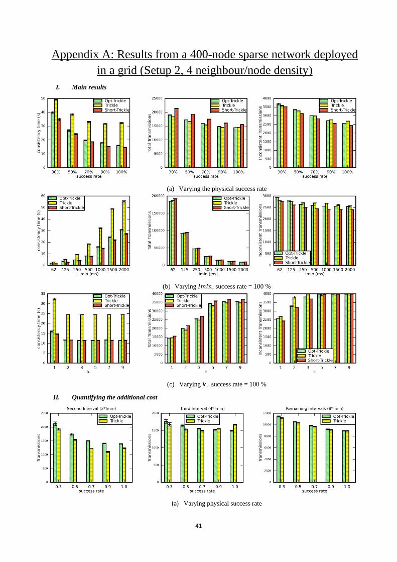
41

Appendix A: Results from a 400-node sparse network deployed

in a grid (Setup 2, 4 neighbour/node density)

I. Main results

(a) Varying the physical success rate

(b) Varying 𝐼𝑚𝑖𝑛, success rate = 100 %

(c) Varying 𝑘, success rate = 100 %

II. Quantifying the additional cost

(a) Varying physical success rate

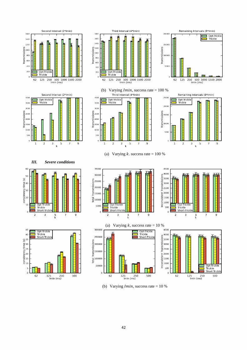
42

(b) Varying 𝐼𝑚𝑖𝑛, success rate = 100 %

(a) Varying 𝑘. success rate = 100 %

III. Severe conditions

(a) Varying 𝑘, success rate = 10 %

(b) Varying 𝐼𝑚𝑖𝑛, success rate = 10 %

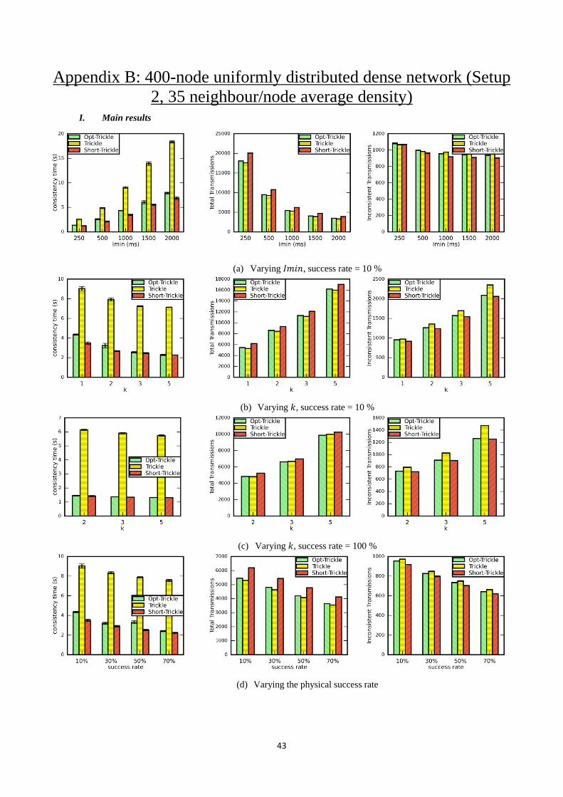
43

Appendix B: 400-node uniformly distributed dense network (Setup

2, 35 neighbour/node average density) I. Main results

(a) Varying 𝐼𝑚𝑖𝑛, success rate = 10 %

(b) Varying 𝑘, success rate = 10 %

(c) Varying 𝑘, success rate = 100 %

(d) Varying the physical success rate

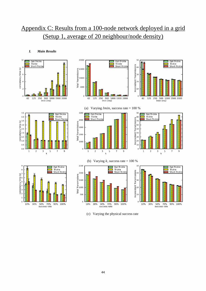
44

Appendix C: Results from a 100-node network deployed in a grid

(Setup 1, average of 20 neighbour/node density)

I. Main Results

(a) Varying 𝐼𝑚𝑖𝑛, success rate = 100 %

(b) Varying 𝑘, success rate = 100 %

(c) Varying the physical success rate

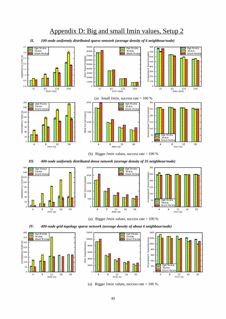
45

Appendix D: Big and small Imin values, Setup 2

II. 100-node uniformly distributed sparse network (average density of 6 neighbour/node)

(a) Small 𝐼𝑚𝑖𝑛, success rate = 100 %

(b) Bigger 𝐼𝑚𝑖𝑛 values, success rate = 100 %

III. 400-node uniformly distributed dense network (average density of 35 neighbour/node)

(a) Bigger 𝐼𝑚𝑖𝑛 values, success rate = 100 %

IV. 400-node grid topology sparse network (average density of about 4 neighbour/node)

(a) Bigger 𝐼𝑚𝑖𝑛 values, success rate = 100 %.

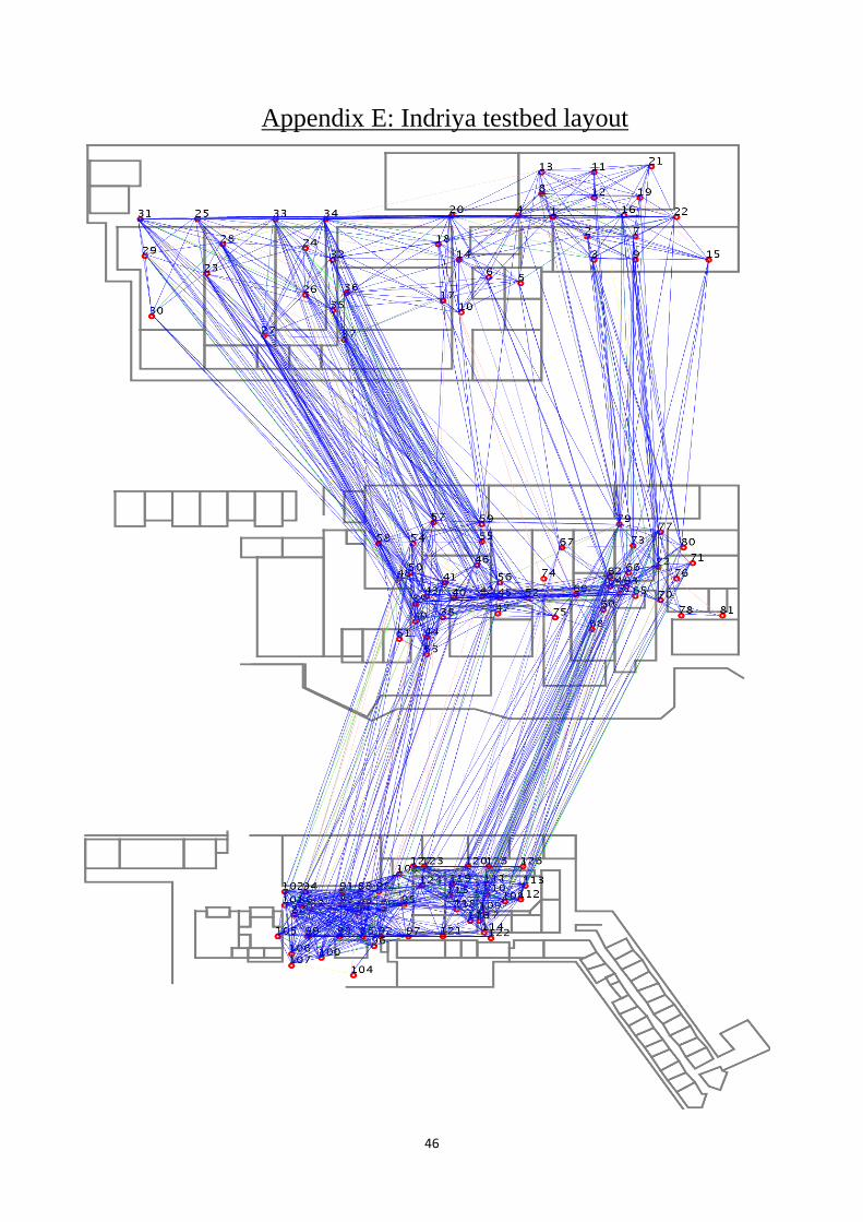
46

Appendix E: Indriya testbed layout