ww.sciencedirect.com

b i o s y s t em s e n g i n e e r i n g 1 1 4 ( 2 0 1 3 ) 8 6e9 6

Available online at w

journal homepage: www.elsevier .com/locate/ issn/15375110

Research Paper

The utility of low-cost photogrammetry for stiffness analysisand finite-element validation of wood with knots in bending

Pablo Guindos*, Juan Ortiz

Department of Agroforestry Engineering, University of Santiago de Compostela, Benigno Ledo 27002 Lugo, Spain

a r t i c l e i n f o

Article history:

Received 9 May 2012

Received in revised form

2 October 2012

Accepted 10 November 2012

Published online 19 December 2012

Abbreviations: DIC, Digital image correlati* Corresponding author. Present address: Dep

38108 Braunschweig, Germany. Tel.: þ49 531E-mail address: pablo.guindos@wki.fraun

1537-5110/$ e see front matter ª 2012 IAgrEhttp://dx.doi.org/10.1016/j.biosystemseng.201

This article presents the capabilities of low-cost photogrammetry as a tool for stiffness

analysis and finite-element (FE) validation in conventional bending tests of structural

timber that contains knots. The accuracy offered by three consumer-grade digital cameras

with a resolution of 10 megapixels was 1/6200, which did not allow for the evaluation of the

stresses or strains in a multiaxial stress field, but provided a thorough contrast of the 3D

nodal displacements, showing the distortion of knots in the modulus of elasticity (MOE), so

that the heterogeneous stiffness of this natural material could be measured and accounted

for. This allowed a more precise determination of the wood stiffness in bending, and

a novel procedure for the estimation of a Clear MOE related to the defect-free areas, an

MOE in Knots related to the distorted regions, and a Global MOE which encompasses both

was developed. The proposed method can be applied to conventional mechanical tests. In

addition, other interesting possibilities for FE validation and monitoring were obtained.

The case study demonstrates how, with a very small investment, an FE model that

simulates the influence of knots in bending could be accurately validated with many fewer

specimens, and how the predictions of displacements could be improved by up to 49%

using the Clear MOE measured by means of the photogrammetry rather than the

conventional MOE without shearing strain.

ª 2012 IAgrE. Published by Elsevier Ltd. All rights reserved.

1. Introduction the key variables of the experiments are measured at only

Wood is a highly heterogeneous material with a very complex

structure, which usually is described as a cylindrical ortho-

tropic composite. The mechanical properties of wood are

strongly affected by the presence of defects, by variations in

density, and by any other inhomogeneities. However, for the

determination of mechanical properties, the validation of

finite-element models, the performance of grading tests, and

other examinations in which destructive tests are required,

on; FE, finite element; MOartment of Construction2155 392; fax: þ49 531 21hofer.de (P. Guindos).. Published by Elsevier Lt2.11.002

a few points on a given specimen. Therefore, a copious

number of samples must compensate for the uncertainty

caused by heterogeneity. This large number of samples can

incur economic and environmental costs in addition to large

investments of time.

The natural solution to this problem should be the

measurement of relevant parameters in the entire sample,

increasing the reliability of each experiment. Thus, close-

range photogrammetry provides a useful tool for obtaining

E, modulus of elasticity.and Structural Engineering, Fraunhofer WKI, Bienroder Weg 54 E,55 200.

d. All rights reserved.

b i o s y s t em s e ng i n e e r i n g 1 1 4 ( 2 0 1 3 ) 8 6e9 6 87

the three-dimensional displacements, strains, stress compo-

nents, or mechanical properties of timber at many points

on each specimen, without the need for direct contact, by

means of digital image correlations (DICs). In recent years,

this technique has been employed in a great number of cases.

For example, Choi, Thorpe, and Hanna (1991) measured

strains and Poisson’s ratios; Masuda, in several studies (e.g.,

Masuda, Iwabuchi, & Murata, 1999; Masuda & Seiichiro, 2004),

evaluated the stresses and strains in small specimens;

Kifetew, Lindberg, and Widlund (1997) measured the strains

during the drying process; Retrieter and Stanzl-Tschegg (2001)

studied the mechanical behaviour of small compressive

specimens by videometry; Franke, Hujer, and Rautenstrauch

(2003) analysed the strain and rupture of small areas of glu-

lam and solid wood using telecentric lenses; Tsakiri,

Papanikos, and Kattis (2004) contrasted the displacement of

structural beams in three-point bending tests; Dahl and Malo

(2008) obtained strains and elastic constants of a sample

under compression using videometry andmeasured the linear

and nonlinear shear properties of spruce (Dahl & Malo, 2009a,

2009b); Sinha and Gupta (2009) analysed the displacement and

strain in shear walls under seismic action; Nagai proposed

defect detection in structural members from the distortion of

a deflection curve (2009) and measured the strain distribution

around a knot during tensile testing (Nagai, Murato, &

Nakano, 2011); and Valla et al. (2011) compared the suit-

ability of Electronic Speckle Pattern Interferometry (ESPI) with

DIC to measure 2D stress distributions in plywood.

In the last decade, consumer-grade digital cameras have

been greatly improved. In addition, as wood is considerably

less stiff compared to other materials, low-cost photogram-

metry could be introduced in timber to evaluate its mechan-

ical properties or carry out FE validations with high accuracy

and little investment.

Therefore, this work evaluates the accuracy achievable

with three consumer-grade 10-megapixel cameras. Once this

parameter is known, the capability of low-cost photogram-

metry for stiffness analysis and FE validation can be deter-

mined in a model that simulates the behaviour of beams with

knots under 4-point bending tests. This analysis includes

a novel determination of the MOE taking into account the

influence of knots in deflection and could be useful for

common flexural grading tests, such as the ASTMD 198 (2003).

2. Materials and methods

2.1. Material

The materials used in this research included nine beams of

3000� 150� 50 mm from Scots pine (Pinus sylvestris L.); a 4-

point bending tester with load and displacement control;

three consumer-grade Canon Eos 400D cameras with resolu-

tions of 3888� 2592 pixels, Canon Inc., �Ota, Tokyo, Japan; five

inductive displacement transducers SM41, Schreiber Mes-

stechnik GmbH, Oberhaching, Germany, with an accuracy of

0.01 mm; commercial FE software, Ansys Multiphysics v11,

Ansys Inc., Canonsburg, PA, USA; PhotoModeler Scanner v6

2.2.596 photogrammetric software and its coded targets, Eos

Systems Inc., Vancouver, BC, Canada; black thumbtacks;

a Metz 45CT flash, Metz-Werke GmbH & Co KG, Zirndorf,

Bavaria, Germany; and one relay and two switches. The total

investment in photogrammetric equipment was approxi-

mately $2900 US dollars.

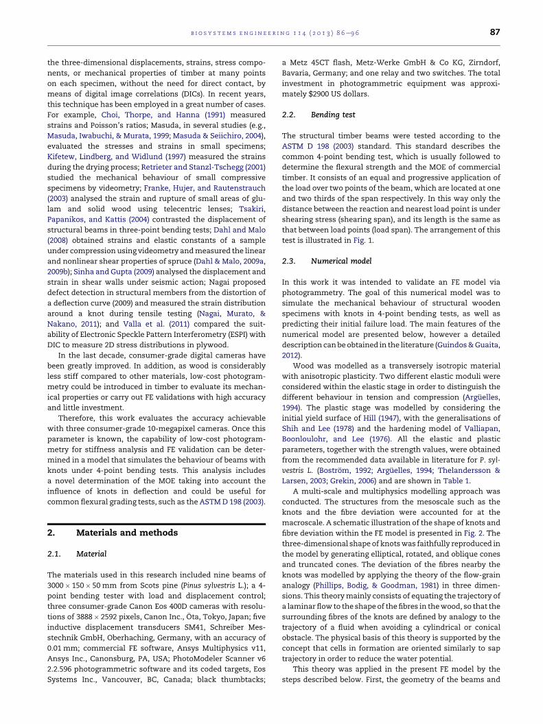
2.2. Bending test

The structural timber beams were tested according to the

ASTM D 198 (2003) standard. This standard describes the

common 4-point bending test, which is usually followed to

determine the flexural strength and the MOE of commercial

timber. It consists of an equal and progressive application of

the load over two points of the beam, which are located at one

and two thirds of the span respectively. In this way only the

distance between the reaction and nearest load point is under

shearing stress (shearing span), and its length is the same as

that between load points (load span). The arrangement of this

test is illustrated in Fig. 1.

2.3. Numerical model

In this work it was intended to validate an FE model via

photogrammetry. The goal of this numerical model was to

simulate the mechanical behaviour of structural wooden

specimens with knots in 4-point bending tests, as well as

predicting their initial failure load. The main features of the

numerical model are presented below, however a detailed

description canbeobtained in the literature (Guindos&Guaita,

2012).

Wood was modelled as a transversely isotropic material

with anisotropic plasticity. Two different elastic moduli were

considered within the elastic stage in order to distinguish the

different behaviour in tension and compression (Arguelles,

1994). The plastic stage was modelled by considering the

initial yield surface of Hill (1947), with the generalisations of

Shih and Lee (1978) and the hardening model of Valliapan,

Boonloulohr, and Lee (1976). All the elastic and plastic

parameters, together with the strength values, were obtained

from the recommended data available in literature for P. syl-

vestris L. (Bostrom, 1992; Arguelles, 1994; Thelandersson &

Larsen, 2003; Grekin, 2006) and are shown in Table 1.

A multi-scale and multiphysics modelling approach was

conducted. The structures from the mesoscale such as the

knots and the fibre deviation were accounted for at the

macroscale. A schematic illustration of the shape of knots and

fibre deviation within the FE model is presented in Fig. 2. The

three-dimensional shape of knotswas faithfully reproduced in

the model by generating elliptical, rotated, and oblique cones

and truncated cones. The deviation of the fibres nearby the

knots was modelled by applying the theory of the flow-grain

analogy (Phillips, Bodig, & Goodman, 1981) in three dimen-

sions. This theorymainly consists of equating the trajectory of

a laminarflow to the shapeof thefibres in thewood, so that the

surrounding fibres of the knots are defined by analogy to the

trajectory of a fluid when avoiding a cylindrical or conical

obstacle. The physical basis of this theory is supported by the

concept that cells in formation are oriented similarly to sap

trajectory in order to reduce the water potential.

This theory was applied in the present FE model by the

steps described below. First, the geometry of the beams and

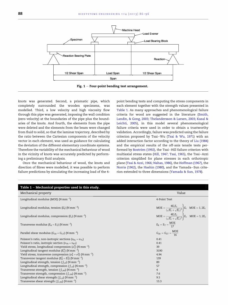
Fig. 1 e Four-point bending test arrangement.

b i o s y s t em s e n g i n e e r i n g 1 1 4 ( 2 0 1 3 ) 8 6e9 688

knots was generated. Second, a prismatic pipe, which

completely surrounded the wooden specimens, was

modelled. Third, a low velocity and high viscosity flow

through this pipe was generated, imposing the wall condition

(zero velocity) at the boundaries of the pipe plus the bound-

aries of the knots. And fourth, the elements from the pipe

were deleted and the elements from the beam were changed

from fluid to solid, so that the laminar trajectory, described by

the ratio between the Cartesian components of the velocity

vector in each element, was used as guidance for calculating

the deviation of the different elementary coordinate systems.

Therefore the variability of themechanical behaviour of wood

in the vicinity of knots was accurately predicted by perform-

ing a preliminary fluid analysis.

Once the mechanical behaviour of wood, the knots and

direction of fibres were modelled, it was possible to perform

failure predictions by simulating the increasing load of the 4-

Table 1 e Mechanical properties used in this study.

Mechanical property

Longitudinal modulus (MOE) (Nmm�2)

Longitudinal modulus, tension (Et) (Nmm�2)

Longitudinal modulus, compression (Ec) (Nmm�2)

Transverse modulus (ER¼ ET) (Nmm�2)

Parallel shear modulus (GLR¼GLT) (Nmm�2)

Poisson’s ratio, non-isotropic sections (vRL¼ vTL)

Poisson’s ratio, isotropic section (vTR¼ vRT)

Yield stress, longitudinal compression (sLY) (Nmm�2)

Longitudinal tangent modulus (ELT) (Nmm�2)

Yield stress, transverse compression (sRY¼ sT

Y) (Nmm�2)

Transverse tangent modulus (ERT¼ ET

T) (Nmm�2)

Longitudinal strength, tension ( ft,0) (Nmm�2)

Longitudinal strength, compression ( fc,0) (Nmm�2)

Transverse strength, tension ( ft,90) (Nmm�2)

Transverse strength, compression ( fc,90) (Nmm�2)

Longitudinal shear strength ( fv,0) (Nmm�2)

Transverse shear strength ( fv,90) (Nmm�2)

point bending tests and computing the stress components in

each element together with the strength values presented in

Table 1. As many approaches and phenomenological failure

criteria for wood are suggested in the literature (Smith,

Landin, & Gong, 2003; Thelandersson & Larsen, 2003; Kasal &

Leichti, 2005), in this model several phenomenological

failure criteria were used in order to obtain a trustworthy

validation. Accordingly, failure was predicted using the failure

criterion proposed by TsaieWu (Tsai & Wu, 1971) with an

added interaction factor according to the theory of Liu (1984)

and the empirical results of the off-axis tensile tests per-

formed by Bostrom (1992), the TsaieHill failure criterion with

multiaxial stress states (Hill, 1947; Tsai, 1965), the TsaieAzzi

criterion simplified for plane stresses in each orthotropic

plane (Tsai & Azzi, 1966; Nahas, 1986), the Hoffman (1967), the

Norris (1962), the Hashin (1980), and the YamadaeSun crite-

rion extended to three dimensions (Yamada & Sun, 1978).

Value

4-Point Test

MOE ¼ 4EtEc

ð ffiffiffiffiffiEt

p þ ffiffiffiffiffiEc

p Þ2)Et MOE ¼ 1; 2Ec

MOE ¼ 4EtEc

ð ffiffiffiffiffiEt

p þ ffiffiffiffiffiEc

p Þ2)Ec MOE ¼ 1; 2Ec

ER ¼ ET ¼ MOE17

GLR ¼ GLT ¼ MOE16

0.41

0.41

39

3190

4.94

139

89

57

4

7.6

9.5

13.3

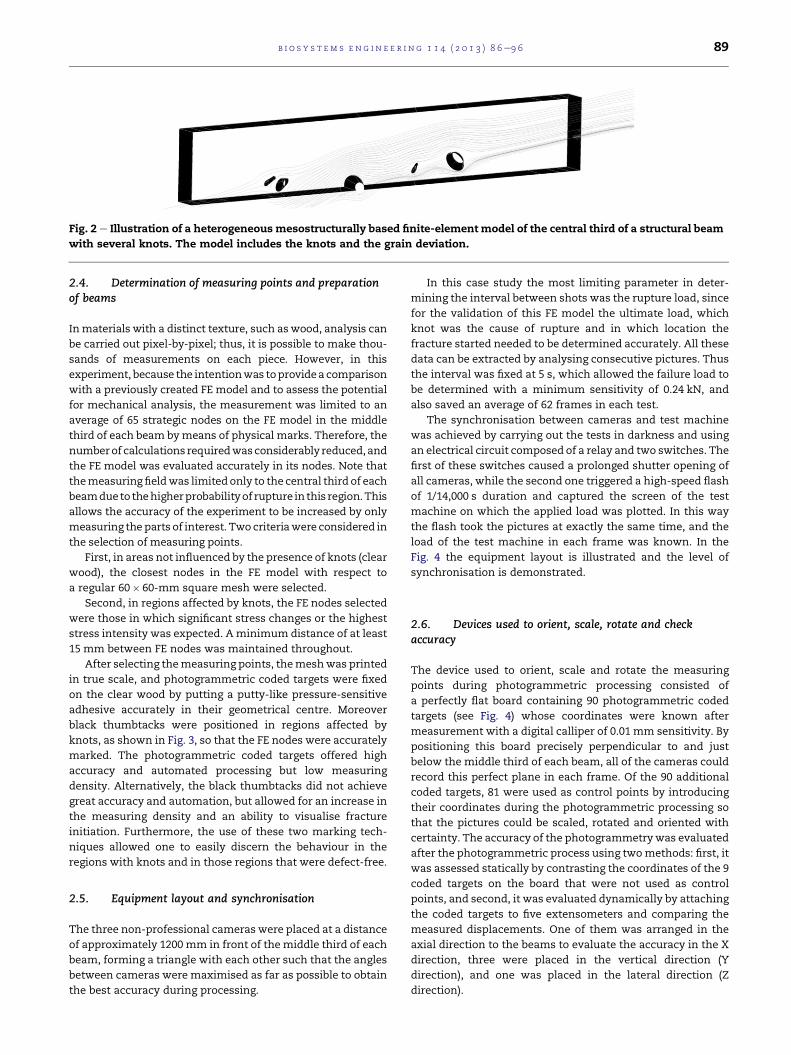
Fig. 2 e Illustration of a heterogeneous mesostructurally based finite-element model of the central third of a structural beam

with several knots. The model includes the knots and the grain deviation.

b i o s y s t em s e ng i n e e r i n g 1 1 4 ( 2 0 1 3 ) 8 6e9 6 89

2.4. Determination of measuring points and preparationof beams

Inmaterials with a distinct texture, such aswood, analysis can

be carried out pixel-by-pixel; thus, it is possible to make thou-

sands of measurements on each piece. However, in this

experiment, because the intentionwas toprovidea comparison

with a previously created FE model and to assess the potential

for mechanical analysis, the measurement was limited to an

average of 65 strategic nodes on the FE model in the middle

third of each beam bymeans of physical marks. Therefore, the

numberof calculations requiredwasconsiderably reduced,and

the FE model was evaluated accurately in its nodes. Note that

themeasuring fieldwas limited only to the central third of each

beamdueto thehigherprobabilityof rupture in this region.This

allows the accuracy of the experiment to be increased by only

measuring the parts of interest. Two criteriawere considered in

the selection of measuring points.

First, in areas not influenced by the presence of knots (clear

wood), the closest nodes in the FE model with respect to

a regular 60� 60-mm square mesh were selected.

Second, in regions affected by knots, the FE nodes selected

were those in which significant stress changes or the highest

stress intensity was expected. A minimum distance of at least

15 mm between FE nodes was maintained throughout.

After selecting themeasuring points, themeshwas printed

in true scale, and photogrammetric coded targets were fixed

on the clear wood by putting a putty-like pressure-sensitive

adhesive accurately in their geometrical centre. Moreover

black thumbtacks were positioned in regions affected by

knots, as shown in Fig. 3, so that the FE nodes were accurately

marked. The photogrammetric coded targets offered high

accuracy and automated processing but low measuring

density. Alternatively, the black thumbtacks did not achieve

great accuracy and automation, but allowed for an increase in

the measuring density and an ability to visualise fracture

initiation. Furthermore, the use of these two marking tech-

niques allowed one to easily discern the behaviour in the

regions with knots and in those regions that were defect-free.

2.5. Equipment layout and synchronisation

The three non-professional cameras were placed at a distance

of approximately 1200 mm in front of themiddle third of each

beam, forming a triangle with each other such that the angles

between cameras were maximised as far as possible to obtain

the best accuracy during processing.

In this case study the most limiting parameter in deter-

mining the interval between shots was the rupture load, since

for the validation of this FE model the ultimate load, which

knot was the cause of rupture and in which location the

fracture started needed to be determined accurately. All these

data can be extracted by analysing consecutive pictures. Thus

the interval was fixed at 5 s, which allowed the failure load to

be determined with a minimum sensitivity of 0.24 kN, and

also saved an average of 62 frames in each test.

The synchronisation between cameras and test machine

was achieved by carrying out the tests in darkness and using

an electrical circuit composed of a relay and two switches. The

first of these switches caused a prolonged shutter opening of

all cameras, while the second one triggered a high-speed flash

of 1/14,000 s duration and captured the screen of the test

machine on which the applied load was plotted. In this way

the flash took the pictures at exactly the same time, and the

load of the test machine in each frame was known. In the

Fig. 4 the equipment layout is illustrated and the level of

synchronisation is demonstrated.

2.6. Devices used to orient, scale, rotate and checkaccuracy

The device used to orient, scale and rotate the measuring

points during photogrammetric processing consisted of

a perfectly flat board containing 90 photogrammetric coded

targets (see Fig. 4) whose coordinates were known after

measurement with a digital calliper of 0.01 mm sensitivity. By

positioning this board precisely perpendicular to and just

below the middle third of each beam, all of the cameras could

record this perfect plane in each frame. Of the 90 additional

coded targets, 81 were used as control points by introducing

their coordinates during the photogrammetric processing so

that the pictures could be scaled, rotated and oriented with

certainty. The accuracy of the photogrammetrywas evaluated

after the photogrammetric process using twomethods: first, it

was assessed statically by contrasting the coordinates of the 9

coded targets on the board that were not used as control

points, and second, it was evaluated dynamically by attaching

the coded targets to five extensometers and comparing the

measured displacements. One of them was arranged in the

axial direction to the beams to evaluate the accuracy in the X

direction, three were placed in the vertical direction (Y

direction), and one was placed in the lateral direction (Z

direction).

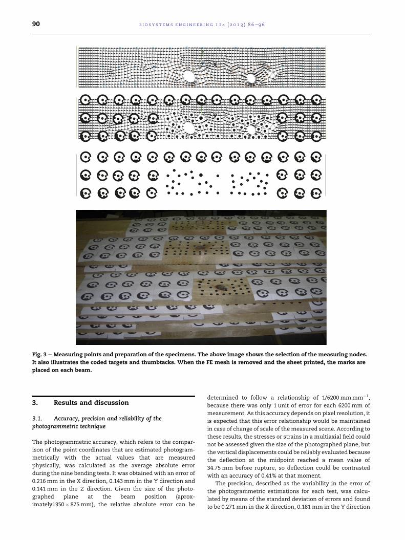
Fig. 3 e Measuring points and preparation of the specimens. The above image shows the selection of the measuring nodes.

It also illustrates the coded targets and thumbtacks. When the FE mesh is removed and the sheet printed, the marks are

placed on each beam.

b i o s y s t em s e n g i n e e r i n g 1 1 4 ( 2 0 1 3 ) 8 6e9 690

3. Results and discussion

3.1. Accuracy, precision and reliability of thephotogrammetric technique

The photogrammetric accuracy, which refers to the compar-

ison of the point coordinates that are estimated photogram-

metrically with the actual values that are measured

physically, was calculated as the average absolute error

during the nine bending tests. It was obtained with an error of

0.216 mm in the X direction, 0.143 mm in the Y direction and

0.141 mm in the Z direction. Given the size of the photo-

graphed plane at the beam position (aprox-

imately1350� 875 mm), the relative absolute error can be

determined to follow a relationship of 1/6200 mmmm�1,

because there was only 1 unit of error for each 6200 mm of

measurement. As this accuracy depends on pixel resolution, it

is expected that this error relationship would be maintained

in case of change of scale of themeasured scene. According to

these results, the stresses or strains in a multiaxial field could

not be assessed given the size of the photographed plane, but

the vertical displacements could be reliably evaluated because

the deflection at the midpoint reached a mean value of

34.75 mm before rupture, so deflection could be contrasted

with an accuracy of 0.41% at that moment.

The precision, described as the variability in the error of

the photogrammetric estimations for each test, was calcu-

lated by means of the standard deviation of errors and found

to be 0.271 mm in the X direction, 0.181 mm in the Y direction

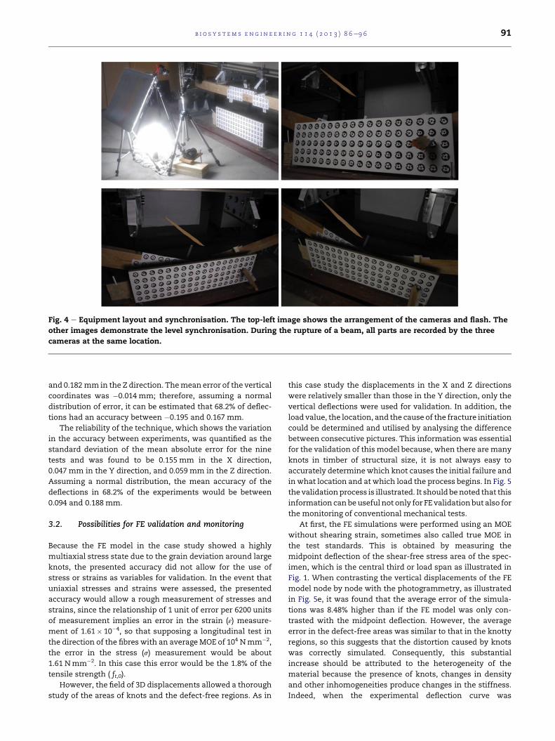
Fig. 4 e Equipment layout and synchronisation. The top-left image shows the arrangement of the cameras and flash. The

other images demonstrate the level synchronisation. During the rupture of a beam, all parts are recorded by the three

cameras at the same location.

b i o s y s t em s e ng i n e e r i n g 1 1 4 ( 2 0 1 3 ) 8 6e9 6 91

and 0.182 mm in the Z direction. Themean error of the vertical

coordinates was �0.014 mm; therefore, assuming a normal

distribution of error, it can be estimated that 68.2% of deflec-

tions had an accuracy between �0.195 and 0.167 mm.

The reliability of the technique, which shows the variation

in the accuracy between experiments, was quantified as the

standard deviation of the mean absolute error for the nine

tests and was found to be 0.155 mm in the X direction,

0.047 mm in the Y direction, and 0.059 mm in the Z direction.

Assuming a normal distribution, the mean accuracy of the

deflections in 68.2% of the experiments would be between

0.094 and 0.188 mm.

3.2. Possibilities for FE validation and monitoring

Because the FE model in the case study showed a highly

multiaxial stress state due to the grain deviation around large

knots, the presented accuracy did not allow for the use of

stress or strains as variables for validation. In the event that

uniaxial stresses and strains were assessed, the presented

accuracy would allow a rough measurement of stresses and

strains, since the relationship of 1 unit of error per 6200 units

of measurement implies an error in the strain (ε) measure-

ment of 1.61� 10�4, so that supposing a longitudinal test in

the direction of the fibres with an averageMOE of 104 Nmm�2,

the error in the stress (s) measurement would be about

1.61 Nmm�2. In this case this error would be the 1.8% of the

tensile strength ( ft,0).

However, the field of 3D displacements allowed a thorough

study of the areas of knots and the defect-free regions. As in

this case study the displacements in the X and Z directions

were relatively smaller than those in the Y direction, only the

vertical deflections were used for validation. In addition, the

load value, the location, and the cause of the fracture initiation

could be determined and utilised by analysing the difference

between consecutive pictures. This information was essential

for the validation of this model because, when there aremany

knots in timber of structural size, it is not always easy to

accurately determinewhich knot causes the initial failure and

in what location and at which load the process begins. In Fig. 5

the validationprocess is illustrated. It should benoted that this

information can beuseful not only for FE validationbut also for

the monitoring of conventional mechanical tests.

At first, the FE simulations were performed using an MOE

without shearing strain, sometimes also called true MOE in

the test standards. This is obtained by measuring the

midpoint deflection of the shear-free stress area of the spec-

imen, which is the central third or load span as illustrated in

Fig. 1. When contrasting the vertical displacements of the FE

model node by node with the photogrammetry, as illustrated

in Fig. 5e, it was found that the average error of the simula-

tions was 8.48% higher than if the FE model was only con-

trasted with the midpoint deflection. However, the average

error in the defect-free areas was similar to that in the knotty

regions, so this suggests that the distortion caused by knots

was correctly simulated. Consequently, this substantial

increase should be attributed to the heterogeneity of the

material because the presence of knots, changes in density

and other inhomogeneities produce changes in the stiffness.

Indeed, when the experimental deflection curve was

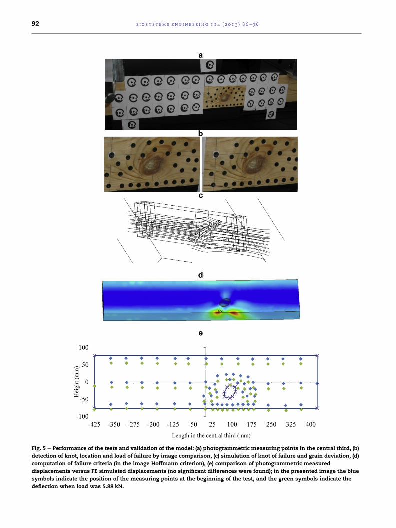
Fig. 5 e Performance of the tests and validation of the model: (a) photogrammetric measuring points in the central third, (b)

detection of knot, location and load of failure by image comparison, (c) simulation of knot of failure and grain deviation, (d)

computation of failure criteria (in the image Hoffmann criterion), (e) comparison of photogrammetric measured

displacements versus FE simulated displacements (no significant differences were found); in the presented image the blue

symbols indicate the position of the measuring points at the beginning of the test, and the green symbols indicate the

deflection when load was 5.88 kN.

b i o s y s t em s e n g i n e e r i n g 1 1 4 ( 2 0 1 3 ) 8 6e9 692

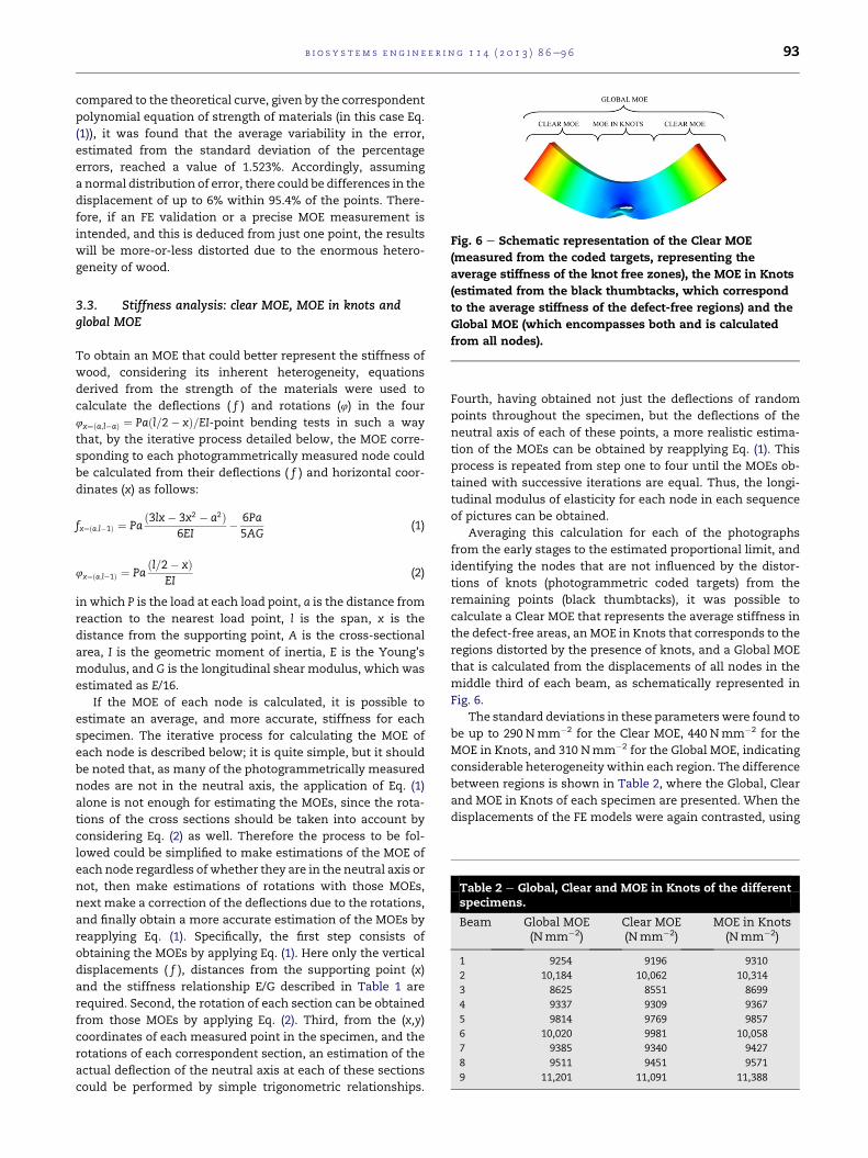
Fig. 6 e Schematic representation of the Clear MOE

(measured from the coded targets, representing the

average stiffness of the knot free zones), the MOE in Knots

b i o s y s t em s e ng i n e e r i n g 1 1 4 ( 2 0 1 3 ) 8 6e9 6 93

compared to the theoretical curve, given by the correspondent

polynomial equation of strength of materials (in this case Eq.

(1)), it was found that the average variability in the error,

estimated from the standard deviation of the percentage

errors, reached a value of 1.523%. Accordingly, assuming

a normal distribution of error, there could be differences in the

displacement of up to 6% within 95.4% of the points. There-

fore, if an FE validation or a precise MOE measurement is

intended, and this is deduced from just one point, the results

will be more-or-less distorted due to the enormous hetero-

geneity of wood.

(estimated from the black thumbtacks, which correspond

to the average stiffness of the defect-free regions) and the

Global MOE (which encompasses both and is calculated

from all nodes).

Table 2 e Global, Clear and MOE in Knots of the differentspecimens.

Beam Global MOE(Nmm�2)

Clear MOE(Nmm�2)

MOE in Knots(Nmm�2)

1 9254 9196 9310

2 10,184 10,062 10,314

3 8625 8551 8699

4 9337 9309 9367

5 9814 9769 9857

6 10,020 9981 10,058

7 9385 9340 9427

8 9511 9451 9571

9 11,201 11,091 11,388

3.3. Stiffness analysis: clear MOE, MOE in knots andglobal MOE

To obtain an MOE that could better represent the stiffness of

wood, considering its inherent heterogeneity, equations

derived from the strength of the materials were used to

calculate the deflections ( f ) and rotations (4) in the four

4x¼ða;l�aÞ ¼ Paðl=2� xÞ=EI-point bending tests in such a way

that, by the iterative process detailed below, the MOE corre-

sponding to each photogrammetrically measured node could

be calculated from their deflections ( f ) and horizontal coor-

dinates (x) as follows:

fx¼ða;l�1Þ ¼ Pað3lx� 3x2 � a2Þ

6EI� 6Pa5AG

(1)

4x¼ða;l�1Þ ¼ Paðl=2� xÞ

EI(2)

in which P is the load at each load point, a is the distance from

reaction to the nearest load point, l is the span, x is the

distance from the supporting point, A is the cross-sectional

area, I is the geometric moment of inertia, E is the Young’s

modulus, and G is the longitudinal shear modulus, which was

estimated as E/16.

If the MOE of each node is calculated, it is possible to

estimate an average, and more accurate, stiffness for each

specimen. The iterative process for calculating the MOE of

each node is described below; it is quite simple, but it should

be noted that, as many of the photogrammetrically measured

nodes are not in the neutral axis, the application of Eq. (1)

alone is not enough for estimating the MOEs, since the rota-

tions of the cross sections should be taken into account by

considering Eq. (2) as well. Therefore the process to be fol-

lowed could be simplified to make estimations of the MOE of

each node regardless of whether they are in the neutral axis or

not, then make estimations of rotations with those MOEs,

next make a correction of the deflections due to the rotations,

and finally obtain a more accurate estimation of the MOEs by

reapplying Eq. (1). Specifically, the first step consists of

obtaining the MOEs by applying Eq. (1). Here only the vertical

displacements ( f ), distances from the supporting point (x)

and the stiffness relationship E/G described in Table 1 are

required. Second, the rotation of each section can be obtained

from those MOEs by applying Eq. (2). Third, from the (x,y)

coordinates of each measured point in the specimen, and the

rotations of each correspondent section, an estimation of the

actual deflection of the neutral axis at each of these sections

could be performed by simple trigonometric relationships.

Fourth, having obtained not just the deflections of random

points throughout the specimen, but the deflections of the

neutral axis of each of these points, a more realistic estima-

tion of the MOEs can be obtained by reapplying Eq. (1). This

process is repeated from step one to four until the MOEs ob-

tained with successive iterations are equal. Thus, the longi-

tudinal modulus of elasticity for each node in each sequence

of pictures can be obtained.

Averaging this calculation for each of the photographs

from the early stages to the estimated proportional limit, and

identifying the nodes that are not influenced by the distor-

tions of knots (photogrammetric coded targets) from the

remaining points (black thumbtacks), it was possible to

calculate a Clear MOE that represents the average stiffness in

the defect-free areas, an MOE in Knots that corresponds to the

regions distorted by the presence of knots, and a Global MOE

that is calculated from the displacements of all nodes in the

middle third of each beam, as schematically represented in

Fig. 6.

The standard deviations in these parameters were found to

be up to 290 Nmm�2 for the Clear MOE, 440 Nmm�2 for the

MOE in Knots, and 310 Nmm�2 for the Global MOE, indicating

considerable heterogeneity within each region. The difference

between regions is shown in Table 2, where the Global, Clear

and MOE in Knots of each specimen are presented. When the

displacements of the FE models were again contrasted, using

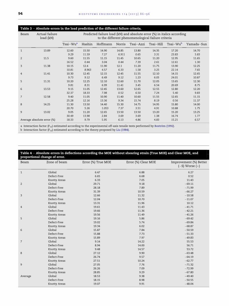
Table 3 e Absolute errors in the load prediction of the different failure criteria.

Beam Actual failureload (kN)

Predicted failure load (kN) and absolute error (%) in italics accordingto the different phenomenological failure criteria

TsaieWua Hashin Hoffmann Norris TsaieAzzi TsaieHill TsaieWub YamadaeSun

1 13.89 12.60 15.50 14.90 14.85 13.80 14.35 17.20 14.70

9.29 11.59 7.27 6.911 0.65 3.31 23.83 5.83

2 11.5 9.60 11.55 11.15 11.45 10.65 11.20 12.95 11.65

16.52 0.44 3.04 0.44 7.39 2.61 12.61 1.30

3 11.38 10.15 12.4 11.90 12.1 11.20 11.75 13.90 12.25

10.81 8.963 4.57 6.33 1.58 3.25 22.14 7.65

4 11.41 10.30 12.45 12.15 12.45 11.55 12.10 14.15 12.65

9.73 9.12 6.49 9.12 1.23 6.05 24.01 10.87

5 11.31 10.20 12.25 12.10 12.60 11.70 12.05 13.65 12.30

9.81 8.31 6.99 11.41 3.45 6.54 20.69 8.75

6 13.53 9.15 11.05 12.45 13.60 12.65 12.55 12.80 12.20

32.37 18.33 7.98 0.52 6.50 7.24 5.40 9.83

7 12.58 9.40 11.05 10.90 11.40 10.60 11.55 12.65 11.15

25.28 12.16 13.36 9.34 15.74 8.19 0.56 11.37

8 14.25 11.30 13.50 14.40 15.30 14.75 14.95 15.80 14.00

20.70 5.26 1.053 7.37 3.51 4.91 10.88 1.75

9 13.02 9.05 11.20 12.65 13.50 13.50 13.20 15.20 13.25

30.49 13.98 2.84 3.69 3.69 1.38 16.74 1.77

Average absolute error (%) 18.33 9.79 5.95 6.13 4.86 4.83 15.21 6.57

a Interaction factor (F12) estimated according to the experimental off-axis tensile tests performed by Bostrom (1992).

b Interaction factor (F12) estimated according to the theory proposed by Liu (1984).

Table 4 e Absolute errors in deflections according the MOE without shearing strain (True MOE) and Clear MOE, andproportional change of error.

Beam Zone of beam Error (%) True MOE Error (%) Clear MOE Improvement (%) Better(�S) Worse (þ)

1 Global 6.47 6.88 6.27

Defect-Free 6.65 6.68 0.52

Knotty Areas 6.33 7.05 11.43

2 Global 29.71 9.18 �69.11

Defect-Free 28.18 7.89 �71.99

Knotty Areas 31.39 10.59 �66.27

3 Global 12.66 11.32 �10.58

Defect-Free 12.04 10.70 �11.07

Knotty Areas 13.31 11.96 10.12

4 Global 19.61 11.43 �41.71

Defect-Free 19.66 11.36 �42.21

Knotty Areas 19.56 11.49 �41.26

5 Global 19.16 5.86 �69.42

Defect-Free 19.02 5.74 �69.84

Knotty Areas 19.34 6.02 �68.87

6 Global 15.87 7.84 �50.59

Defect-Free 15.88 7.73 �51.33

Knotty Areas 15.89 7.97 �49.83

7 Global 9.14 14.22 55.53

Defect-Free 8.94 14.00 56.71

Knotty Areas 9.48 14.57 53.72

8 Global 27.12 9.90 �63.48

Defect-Free 26.74 9.57 �64.19

Knotty Areas 27.51 10.24 �62.77

9 Global 27.05 7.76 �71.32

Defect-Free 26.26 7.09 �72.99

Knotty Areas 28.85 9.29 �67.80

Average Global 18.53 9.38 �49.40

Defect-Free 18.15 8.98 �50.55

Knotty Areas 19.07 9.91 �48.04

b i o s y s t em s e n g i n e e r i n g 1 1 4 ( 2 0 1 3 ) 8 6e9 694

b i o s y s t em s e ng i n e e r i n g 1 1 4 ( 2 0 1 3 ) 8 6e9 6 95

the Clear MOE instead of the MOE calculated from the

deflection at the midpoint in the simulations in accordance

with the test standards, the average improvement in the

estimations was found to be greater than 49%.

Note that the results of Table 2may be opposite to intuitive

thinking since the MOE in Knots was clearly greater that the

Clear MOE. However, the distortion of the deflection curve at

the knotty areas in the reality was found to be as represented

schematically in Fig. 6. In the knotty areas the local distortion

of knots generated a decrease of the deflections so that the

MOE was higher in all the cases. These results converge with

the data presented by Nagai et al. (2009) for encased knots in

tension zones as in the case study.

3.4. Results of FE simulations

The absolute errors according to the different phenomeno-

logical criteria in the failure prediction are presented in Table

3. The errors in the displacement prediction according to the

MOE without shearing strain and the Clear MOE, and the

relative changes are shown in Table 4. The TsaieHill criterion

provided the best failure predictions with an average absolute

error of 4.83%. The average error in displacements was 9.38%

within the central third of the beams. Specifically, the error in

the defect-free areas was 8.98% and the error in the knotty

zones was 9.91%. The small difference between defect-free

and knotty areas suggest a right simulation of the knots and

their nearby fibres. Note that all these errors are the average

errors of the 65 measured points of each central third. The

improvement of simulationswhen using the ClearMOE rather

than MOE according standard tests was about 49%.

4. Conclusions

With a small investment, a photogrammetric technique was

developed that offered an accuracy of 1/6200 mm mm�1 by

using three consumer-grade 10-megapixel cameras. The

precision, the reliability and the synchronisation of the pre-

sented method were all quite satisfactory. These parameters

are improved if the low stiffness of the wood is taken into

account.Given the sizeof the tests, itwasnotpossible toassess

stresses or strains in amultiaxial stress state, but the obtained

information was essential to thoroughly contrast the three-

dimensional displacements of a field of FE nodes, dis-

tinguishingbetween theeffects of regionsof knots and thoseof

defect-free areas. The information also enabled an accurate

determination of the cause, the load, and the location of the

initial fracture so that the uncertainty produced by the

heterogeneity of the wood was significantly decreased, allow-

ing a much more trustworthy FE validation. It was expected,

that without photogrammetry, the simulation of this case

study would have required a very large number of tests before

one could reach reliable conclusions regarding the validation,

so that the requirednumber of testswas considerably reduced.

When the field of displacements of the FE model was

thoroughly contrasted using the conventional MOE without

shearing strain, the average error was nearly 8.5% higher than

that when only the deflection at the midpoint was compared.

A high heterogeneity in the displacement field was found for

beams with significant defects, such as knots and other

inhomogeneities. In these cases, the real deflection curve

could be considerably distorted with respect to the theoretical

one, and the stiffness could vary considerably within and

between small regions.

Therefore this research proposes a novel determination of

stiffness in order to deal with this heterogeneity. First there

where discerned 3 different stiffnesses in thewood: the Global

MOE, the Clear MOE, and the MOE in Knots. These three

moduli try to show the difference between the stiffness of

knotty and defect-free parts of wood. The Clear MOE is

measured only in the defect-free parts where there is no

distortion in the elasticity due to the knots. Conversely, the

MOE in Knots only accounts for the elasticity of the knotty

parts. The Global MOE encompasses both regions and repre-

sents the average stiffness of a specimen. Additionally, the

heterogeneity not between but within each of these areas was

also taken into account by measuring the MOE throughout

a mesh of points in each area. This entire rigorous proposal

about wood stiffness is recommended when analysing

measurable aspects of wood, such as the validation of FE

models. In the case study the performance of an FE model

improved by up to 49% when using the Clear MOE, instead of

the conventional MOE without shearing strain, which is

usually used in the test standards.

The weakness of the proposedmethod was in the low auto-

mation of the entire process, especially sample preparation.

However, thousands of data points could be obtained, which

were very useful for the FE validations, allowing a wide range of

comparisons from just 9 specimens. Furthermore, as the accu-

racy of digital cameras continues to increase in the coming

years, and as the presented process can be further automated,

the concepts of stiffness presented in this article could be

cheaply and easily extended tomore conventional uses, such as

tests used formechanical characterisation of timber. Therefore,

themeasurementofMOEcouldbe improvedto take intoaccount

theeffectofheterogeneity.This researchbecomesmoreuseful if

one takes intoaccount the fact thatmanymechanical properties

are estimated from this elastic parameter.

Acknowledgements

The authors acknowledge the support of the Spanish Ministry

of Education for its financial support through the National

Training Program of University Lecturers (FPU).

r e f e r e n c e s

ASTM D 198e199 (2003). Standard test methods of static tests oflumber in structural sizes. Annual Book of ASTM Standards,Vol 04.10. West Conshohocken, PA.

Arguelles B (1994). Prediccion con simulacion animada delcomportamiento de piezas de Madera. Dissertation (inSpanish), Polytechnic University of Madrid, Madrid, Spain.

Bostrom L (1992) Method for determination of the softeningbehavior of wood and the applicability of a non linear fracturemechanicsmodel. Dissertation, LundUniversity, Lund, Sweden.

b i o s y s t em s e n g i n e e r i n g 1 1 4 ( 2 0 1 3 ) 8 6e9 696

Choi, D., Thorpe, J. L., & Hanna, R. B. (1991). Image analysis tomeasure strain in wood and paper. Wood Science andTechnology, 25, 251e262.

Dahl, K. B., & Malo, K. A. (2008). Planar strain measurements onwood specimens. Experimental Mechanics, 49, 575e586.

Dahl, K. B., & Malo, K. A. (2009a). Linear shear properties of sprucesoftwood. Wood Science and Technology, 43, 499e525.

Dahl, K. B., & Malo, K. A. (2009b). Nonlinear shear properties ofspruce softwood: experimental results. Wood Science andTechnology, 43, 539e558.

Franke B; Hujer S; Rautenstrauch K; (2003). Strain analysis of solidwood and glued laminated timber constructions by closerange photogrammetry. International Symposium of Non-Destructive Testing in Civil Engineering, 16e19 September,Berlin, Germany.

Grekin, M. (2006). Nordic Scots pine vs. selected competing species andnon-wood substitute materials in mechanical wood products.Literature surveyIn Working Papers of the Finnish Forest ResearchInstitute, vol. 36. Finland: Finnish Forest Research Institute.

Guindos P; Guaita M (2012). A three-dimensional wood materialmodel to simulate the behavior of wood with any type of knotat the macro-scale. Wood Science and Technology, (in press).

Hashin, Z. (1980). Failure criteria for unidirectional fibercomposites. Journal of Applied Mechanics e Transactions of ASME,47, 329e334.

Hill, R. (1947). A theory of the yielding and plastic flow ofanisotropic metals. Philosophical Transactions of the Royal SocietyA, 193, 281e297.

Hoffman, O. (1967). The brittle strength of orthotropic materials.Journal of Composite Materials, 1, 200e206.

Kasal, B., & Leichti, R. J. (2005). State of the art in multiaxialphenomenological failure criteria for wood members. Progressin Structural Engineering and Materials, 7, 3e13.

Kifetew, G., Lindberg, H., & Wiklund, M. (1997). Tangential andradial deformation field measurements on wood duringdrying. Wood Science and Technology, 31, 35e44.

Liu, J. Y. (1984). Evaluation of the tensor polynomial strengththeory for wood. Journal of Composite Materials, 18, 216e226.

Masuda M; Iwabuchi A; Murata K (1999). Analyses of fracturecriteria using image correlation method. Proceedings of FirstRilem Symposium on Timber Engineering, 13-15 September,Stockholm, Sweden, pp 151e160.

Masuda, M., & Seiichiro, U. (2004). Investigation of the truestressestrain relation in shear using the digital imagecorrelation method. Mokuzai Gakkaishi, 50, 146e150.

Nagai, H., Murata, K., & Nakano, T. (2009). Defect detection inlumber including knots using bending deflection curve:

comparison between experimental analysis and finiteelement modeling. Journal of Wood Science, 55, 169e174.

Nagai, H., Murata, K., & Nakano, T. (2011). Strain analysis oflumber containing a knot during tensile failure. Journal of WoodScience, 57, 114e118.

Nahas, M. N. (1986). Survey of failure and post-failure theories oflaminated fiber-reinforced composites. Journal of CompositesTechnology and Research, 8, 138e153.

Norris, C. B. (1962). Strength of orthotropic materials subjected tocombined stresses. Report No. 1816. Madison, WI, USA: USForest Products Laboratory.

Phillips, G. E., Bodig, J., & Goodman, J. R. (1981). Flow grainanalogy. Wood Science and Technology, 14, 55e64.

Retrieter, A., & Stanzl-Tschegg, S. E. (2001). Compressivebehaviour of softwood under uniaxial loading at differentorientations to the grain. Mechanics of Materials, 33, 705e715.

Shih, C. F., & Lee, D. (1978). Further developments in anisotropicplasticity. Journal of Engineering Materials and Transactions of theASME, 100, 294e302.

Sinha, A., & Gupta, R. (2009). Strain distribution in OSB and GWBin wood-frame shear walls. Journal of Structural Engineering-ASCE, 135, 666e675.

Smith, I., Landis, E., & Gong, M. (2003). Fracture and fatigue in wood(first ed.). West Sussex, UK: Wiley.

Thelandersson, S., & Larsen, H. J. (2003). Timber Engineering. WestSussex, UK: Wiley.

Tsai, S. W. (1965). Strength characteristics of composite materials.NASA Report No. CR-224, Washington DC, USA.

Tsai, S. W., & Azzi, V. D. (1966). Strength of laminated compositematerials. AIAA Journal, 4, 296e301.

Tsai, S. W., & Wu, E. M. (1971). A general theory of strength foranisotropic materials. Journal of Composite Materials, 5, 58e80.

Tsakiri I; Papanikos P; Kattis M (2004). Load testing measurementsfor structural assessment using geodetic andphotogrammetric techniques. First international symposiumon engineering surveys for construction works and structuralengineering, Nottingham, UK.

Valla, A., Konnerth, J., Keunecke, D., Niemz, P., Muller, U., &Gindl, W. (2011). Comparison of two optical methods forcontactless, full field and highly sensitive in-planedeformation measurements using the example of plywood.Wood Science and Technology, 45, 755e765.

Valliappan, S., Boonlaulohr, P., & Lee, I. K. (1976). Non-linearanalysis for anisotropic materials. International Journal ofNumerical Methods in Engineering, 10, 597e606.

Yamada, S. E., & Sun, C. T. (1978). Analysis of laminate strengthand its distribution. Journal of Composite Materials, 12, 275e284.