The virtual slice setup

The Virtual Slice Setup

William W Lytton1,2,*, Samuel A Neymotin2, and Michael L Hines3

1 Dept. of Physiology, Pharmacology, Neurology, SUNY Downstate, Brooklyn, NY

2 Dept. of Biomedical Engineering, SUNY Downstate, Brooklyn, NY

3 Dept. of Computer Science, Yale University, New Haven, CT

AbstractIn an effort to design a simulation environment that is more similar to that of neurophysiology, weintroduce a virtual slice setup in the NEURON simulator. The virtual slice setup runs continuouslyand permits parameter changes including changes to synaptic weights and time course and to intrinsiccell properties. The virtual slice setup permits shocks to be applied at chosen locations and activityto be sampled intra- or extracellularly from chosen locations. By default, a summed populationdisplay is shown during a run to indicate the level of activity and no states are saved. Simulationscan run for hours of model time, therefore it is not practical to save all of the state variables whichin any case are primarily of interest at discrete times when experiments are being run: the simulationcan be stopped momentarily at such times to save activity patterns. The virtual slice setup maintainsan automated notebook showing shocks and parameter changes as well as user comments. Wedemonstrate how interaction with a continuously running simulation encourages experimentalprototyping and can suggest additional dynamical features such as ligand wash-in and wash-out –alternatives to typical instantaneous parameter change. The virtual slice setup currently uses event-driven cells and runs at approximately 2 minutes/hour on a laptop.

Keywordscomputer simulation; computer modeling; neuronal networks; electrophysiology

IntroductionNeural simulation has traditionally been practiced more like American rather than likeinternational football: discrete simulations followed by regrouping and reorganization toprepare for the next attempt. This method necessarily distances the practice of simulation fromin vivo neurophysiology, where experiments are performed on an active dynamical systemwhich is never truly statistically stationary. It is more similar to performing experiments on aquiescent brain slice that requires repeated shocks to produce transient activity but againdissimilar to slice experiments on an active, firing network – an “epileptic” slice.

An alternative to the traditional simulation method has been called reactive animation (RA)by Efroni and colleagues (2005, 2007). The “reactive” refers to reactive systems, a termoriginating in engineering and now being introduced in biology. In engineering, reactivesystems can be distinguished from transformational systems, which are designed to terminatein a distinct output. Reactive systems, by contrast, operate in real-time (e.g., cruise controls

*Corresponding author: 450 Clarkson Ave, Box 31, Bklyn, NY 11203-2098 tel 718 270 6789, fax: 815 642 4019, email:[email protected].

NIH Public AccessAuthor ManuscriptJ Neurosci Methods. Author manuscript; available in PMC 2009 June 30.

Published in final edited form as:J Neurosci Methods. 2008 June 30; 171(2): 309–315. doi:10.1016/j.jneumeth.2008.03.005.

NIH

-PA Author Manuscript

NIH


NIH


and autopilots) and produce outputs that are state dependent. A particular output is only correctwhen it is produced at the correct time: the reactive system is in a continuous dynamicalinterplay with its environment. Seen in these terms, all biological systems are reactive systems.A biological system is continuously evolving, reacting to inputs that may also alter the systemitself (plasticity). As with aircraft or process engineering, a reactive, real-time, ongoingbiological system may be best served by use of reactive simulation.

The “animation” of reactive animation is obligatory rather than cosmetic: it provides the meansfor interaction with the running simulation, providing continuous or statistical evaluation ofstate variables and allowing control of system parameters. Like a video game, the quality ofthe simulation experience depends largely on the adherence to both the pragmatics and thedynamics of the system. As we will show, the experience of immediate interaction with thesimulation can lead one to make improvements to this realism. However, neurophysiologicalsimulation still suffers from a severe lack of detail compared to engineering systems or evenother biological preparations. In particular, there is a lack of detailed wiring information forbrain areas, contrasting markedly with the relatively sophisticated knowledge of the singleneuron.

Compared to experiment, simulation offers advantages of detailed observability and control.One has the ability to see all voltages and concentrations and to manipulate anyneurotransmitter or ion channel at will. Indeed, one of the difficult problems in designing anRA simulator is adapting the graphical environment to the user, showing the user necessaryinformation for a particular experiment without overwhelming him with extraneous data ormultiple control panels.

Although the formalized notions of RA are relatively new to biology, the idea of interactivesimulation in neurophysiology dates back at least to P. Rowat’s “Preparation” simulator. Thislobster stomatogastric ganglion simulator was developed in the late 1980s, only about 5 yearsafter the development of stand-alone graphical workstations made sophisticated graphicsreadily available (Rowat and Selverston 1993). More recently, M. Hereld and collaboratorshave been advancing the idea of interactive simulations running on large parallelsupercomputers in continuous communication with a front-end graphical workstation (Hereldet al. 2007). The virtual slice setup (VS) developed here has the advantage of being fairly large(expandable to about 1 · 105 neurons on a standard workstation) without requiring asupercomputer. Here we illustrate a 2700 cell simulation which runs at approximately 2 modelminutes/hour on a laptop. This simulation rate makes it easy to run ion channel and synapticblockade experiments over periods of several seconds of simulated time.

Materials and MethodsThe techniques and simulations described here are implemented in the NEURON simulator(Neuron web site 2007; Carnevale and Hines 2006) using a rule-based artificial cell mechanism(Lytton and Hines 2004; Lytton and Stewart 2005; Lytton and Stewart 2006). This neuronmodel is a fast event-driven unit that was designed with several of the attributes of biologicalneurons, including adaptation, bursting, depolarization blockade, Mg++-sensitive NMDAconductance, anode-break depolarization, and others.

The unit has 5 state variables: 4 for inputs – Vi for AMPA, NMDA, GABAA (the acronymsrefer here to the dynamics of the associated receptors and not to the chemicals), and 1 intrinsicstate variable – VAHP (afterhyperpolarization following a spike). State variables are onlyupdated when an event, external or internal, is received. External events arrive from otherneurons. Internal events indicate an internal state update: e.g., the end of the refractory period.External events produce a step increment in associated synaptic state variables. A spike

Lytton et al. Page 2

J Neurosci Methods. Author manuscript; available in PMC 2009 June 30.

NIH


NIH


NIH


produces an increment in VAHP. State variables are updated according to a weight parameterWi. This weight is multiplied by a driving force to produce a step voltage increment S:

. WNMDA is scaled by a function of postsynaptic voltage and Mg++ concentration.Wi is a unitless weight, not a conductance. Steps are unidirectional – i.e., reversal of synapticcurrent is not simulated. Si instantaneously updates the associated state variable: Vi += Si.Except at a step, Vi decays with time constant τi. Because state variables decay exponentially,they can be updated analytically at event times. State variables are summed with restingmembrane P potential (RMP) to arrive at a final membrane voltage Vm = Σi Vi for i = {AMPA;NMDA; GABAA; GABAB; AHPg}. Vm is compared to threshold to determine if firing takesplace (comparable to integrate and fire).

Additional parameters and check points are used to provide varying refractory period, bursting,depolarization blockade and other features. Speed-up is obtained through use of table look-upto avoid run-time calculation of exponential decays and other response wave forms.

The network used here is an epileptic network using the event-driven cell type described withthree different parameterizations reflecting three cell types: 1) a small but more excitableexcitatory D (driver) population of 200 cells, that played the role of a driver of activity; 2) alarger excitatory population E (expressor) of 2000 cells, and 3) an inhibitory population I,consisting of 500 cells (Lytton and Omurtag 2007; Lytton et al. 2008a). Connectivity was basedon a random (Renyi-Erdös) directed graph with low connection densities:

Synaptic weights were assigned randomly with a normal distribution around the parametercentral point within a narrow range. Synaptic delays were chosen randomly from a uniformdistribution within a range of 2–3 ms. Individual cell parameters were chosen from distributionsbased around central values for intrinsic parameters, each set differently for the 3 different cellpopulations. Approximate maximal firing rates were approximately 150, 100, and 330 Hz (forD, E, and I cell types respectively), determined dynamically by refractory periods,afterhyperpolarization weights and afterhyperpolarization decay constants.

The full simulation described in this paper is available in runnable open-source form at theModelDB web site (Hines and Carnevale 2004; ModelDB web site 2007). The network is self-sustaining, running continuously without external input and with no intrinsic activity in anycells. Though the sparse random network used is nominally based on values derived from areaCA3 of hippocampus, we are not in the present instance attempting to model specific slicephenomenology.

Simulations were run on an IBM X60 laptop with dual core 1.83 GHz processors,demonstrating simulation feasibility with a moderate-sized machine. Substantially larger



NIH


NIH


NIH


simulations can be run on compute-serve workstations as will be noted below. This is in partdue to savings in computer memory space using the recently developed JitCon (just-in-timeconnectivity) mechanism (Lytton et al. 2008b).

ResultsUsing the virtual slice setup

The default display for the VS consists of only two windows, though with multiple recordingsites and parameter panels the display can quickly grow to encompass many tens of panels.Because the program is profligate in its use of windows, they are grouped so as to allow setsof them to be closed or reopened in concert. The two default windows are population activitydisplay and the control panel (Fig. 1). The activity display (left) shows the total number ofspikes occurring over a customizable integration period (default 10 ms). In the present instance,the graphic suggests that approximately 1700–1900 cells are active out of the 2700 cells in thesimulation. This is therefore a highly active simulation with an average firing frequency ofabout 70 Hz. Since the integration period here is about twice the length of the average refractoryperiod for the individual cell, this spike measure may slightly overestimate the number of activecells due to the rare occurrence of doublet firing during the period. We have used the simplespike count as the standard view, rather than providing a more sophisticated calculation of fieldpotential that would take longer to calculate. We refer to the integrated spike count as a “field”below as a shorthand. As with other interactive computer systems, it’s often necessary to optfor speed over detail in order to allow the user to work with the system in real time.

By default, 1 second of simulation time is shown as a continuous sweep (customizableparameter: field duration). We have run simulations for up to several hours of model time.Saving all the data from one of these simulations would require ~290 MB/model hour/trace atour default 10 kHz sub-sampling. This would also entail frequent writing to disk which wouldagain slow the simulation process. Saving all of the voltage traces from a simulation of thissize would require ~780 GB/model hour and saving all state variables ~3.9 TB/model hour.Instead of continuous saving, the user has the option of saving desired fields, voltages or statevariables on request when a phenomenon of interest is noted or a particular manipulation hasbeen made.

The control panel (Fig. 1 right) has buttons that are largely self-explanatory. The top line is asystem message that generally reflects simulation status, in the present case giving thesimulation name (a customizable string based by default on local time when the simulationwas started) and indicating that the simulation was restarted at 190.5 s in simulation time. Thesimulation can be stopped at any time to permit assessment and to allow further analysis fromthe command line. As with the 10 ms graphical integration time, the buttons are only queriedevery 10 ms by default. This could be readily decreased to a 1 ms interval when using a fastCPU. The Continue button then restarts the simulation. The third button on the control panel,Shock, provides instantaneous activation of a percent of the population in the currentsimulation. Stimulation parameters are customized in a separate panel (not shown).

As described in Methods, the simulation used here has three cell types: a primary excitatorycell considered an Expressor of activity (E cells), a smaller population of higher-excitabilitycells considered activity Drivers (D cells) and a population of inhibitory cells (I cells) (Lyttonand Omurtag 2007). A single cell from any of these populations can be displayed by enteringthe cell number and pressing Graph cell (Fig. 2). Similarly, activity in the population of agiven cell type can be displayed with Graph type. Note that the cell type is represented by asymbolic parameter which resolves to an index number: in the present case the E cells arerepresented by EX (E in Neuron is reserved for the base of the natural logarithm). EX resolvesto 3, so that either “EX” or “3” could be entered next to the button to display the E-cell field.



NIH


NIH


NIH


All graphics can be toggled of (Graphics on/off) to allow the simulation to move forwardmore rapidly, which might be desirable when waiting for a steady state to be reached.

The Show slice button provides clickable views of the slice that permit individual cells orgroups of cells to be interactively chosen for display. It launches multiple views (currently 3)with cells located according to their defined x,y coordinate positions (Fig. 3). In the presentinstance, the cells have been randomly placed at locations within an ellipse; each cell isrepresented by a black dot. The multiple views are available to avoid the crowding andconfusion of superimposed symbols. Each view has different mouse functionality: e.g., theability to position a shock, to launch single cell or field graphics or to launch various kinds ofactivity animations. In Fig. 3, the top view launches graphics. A mouse click on the top viewplaces a colored cross over a cell symbol, e.g., the red cross at the right, and launches a separateline graph with the voltage trace of that cell (here the cell trace in Fig. 2B). Similarly, a mousedrag-event colors in a set of cells within the defined circle and launches an identically-coloredfield trace comparable to the field traces in Fig. 2A. The second view provides local fieldpotential animation: it defines a circle of cells as in the first view but instead of launching atrace produces an animated red ellipse which grows and shrinks vertically with activity in thedefined area. The third view provides a cell-based animation with individual squares showingthe potential in each individual neuron.

When something interesting is seen on the screen, the Save button will launch a Save dialog(Fig. 4). This screen allows 1. entering a free-form comment; 2. changing the output file namestem (default is based on the simulation name and simulation time); 3. selection of one ofseveral formats for saving. All currently displayed fields or cell traces will be saved. These canbe saved either in a graphical or vector formats. Only the currently displayed traces can besaved to disk since other state variables are not being retained in memory. Fig. 2 was saved byselecting the checkbox for Save to idraw which saved directly to the editable postscript formatused by Neuron. The final version of Fig. 2 then required only alignment and labeling of the3 panels.

When the VS is run a notebook, “notes.txt” by default, is maintained which gives the simulationname and any information regarding parameter changes, shocks or file saves. In the case ofFig. 2, the section of notebook reads:

* Sim start at 07Dec18:13:58:35EST

User [email protected]

USER NOTE@t=96.86:For paper

Data written to data/SIM 07Dec18:13:[email protected]

User [email protected]

Here the comment we entered was “for paper” and we have left the unwieldy full file name.The notes.txt file is user-editable text: additional notes can be added from an editor.

Parameter changesFor the present simulation, weight and intrinsic cell parameters have been made available fordirect change via panels. Although additional parameters can be changed by stopping thesimulation, changing a parameter in the interpreter and restarting, this interferes with one’sdynamical sense of activity alteration. In any case, a newly designed parameter panel can belaunched from the interpreter with a single function call. As with the Graph type button, the



NIH


NIH


NIH


Cell params button requires entry of a cell type in either symbolic or numerical form (e.g.,typing either “EX” or “3” for the E-cells). One can of course launch all 3 cell-parameter panels.Uniform or Gaussian variability of individual cell parameters around a central value isprovided; this variability is itself parameterized and could be made interactively available ina panel. We do not currently envision a need to alter the parameters of individual cells directlyrather than as part of a population.

Fig. 5 show the current parameter panels for weights and cell parameters (here for the E cells).The weight parameters are separated by pre- and postsynaptic cell type and by synapse type(i.e., AMPA, NMDA, GABAA; GABAB is not present in this simulation). Some of the cellparameters are actually synaptic – the time constant of AMPA, NMDA or GABAA decay areattributes of the postsynaptic cell. Several points merit further explanation. First, with 3 celltypes the weight panel is barely manageable in length. With more cell types, the scrollbar wouldneed to be used. In practice, we anticipate that the panel would instead be modified to onlydisplay the weights of interest for a particular set of simulations. As noted above, panel contentsare readily altered using function calls from the Neuron simulator interpreter. Second, we havehere altered standard Neuron panel usage in one respect: changing a value and clicking theassociated button does not immediately alter that parameter in the simulation. Instead a changeto a weight parameter produces the following message at the top of the panel: “Press ‘Changeweights’ button for effect.” This additional button press is required in order to permit multipleparameter changes to be effected simultaneously in order to simulate the “dirty” (multiplebinding site) effects of many drugs and endogenous ligands. For this reason, the variousparameter panels can also be linked so that a single button press simultaneously produceschanges in both weights and in intrinsic cell parameters. In practice, a particular simulationmight use e.g., a single “Acetylcholine” button rather than making several alterationsindividually. Third, pressing the top button not only makes the weight changes but alsodocuments the change in the notes.txt notebook, e.g.,

Weight changes @t=29080: E->I:AMPA:0.01->0.05; E->I:NMDA:0.2->0.1; D-

>E:AMPA:0.1->0.2.

Fourth, the values shown in the Weight Panel are unitless scaling factors. As with the cellparameters, the weights are randomized around a central value; rescaling shifts all of theassociated weights affecting their relative strengths. Fifth, the values shown in the cellparameter panel without are in ms (e.g., tauAM –– the AMPA time constant and refrac ––the refractory period) or mV (e.g., RMP –– resting membrane potential and VTH | the firingthreshold). These parameters are specific to the neuron model parameterization being used here(see Methods). The parameters would of course be quite different, and substantially morecomplicated, for a compartmental model. Currently, use of full multi-compartmental model atthis scale is not practical on a single CPU but could be performed in the future using multi-threading or via linkage to a parallel supercomputer (see Discussion).

Advantages of continuous simulationAn advantage of the VS is that usage of this tool tends to suggest further improvements toallow the VS to conform still more closely to experimental physiology practice. This is bestillustrated by the Wash in button near the top of the weight parameters panel (Fig. 5A) whichwas not originally included. The discrepancy with experimental practice was noticeable whenclicking the Change weights button which effected instantaneous alterations in synapticstrengths. Such instantaneous effects are of course not possible in physiology where anexogenous ligand requires time to flow into the chamber, to diffuse into the tissue, to equilibrateat concentration, and to bind to receptors. We therefore added a Wash in/out button whichprovides linear increase or decrease in the changed parameters over the time period given on



NIH


NIH


NIH


the panel (300 ms in Fig. 5A). This adds the simulation of experimental dynamics to that ofphysiological dynamics.

We found that this alteration in parameter-change timing could produce substantial andreproducible effects. Fig. 6 shows a 35% synaptic weight reduction from E to D cells. Thissynaptic strength reduction generally terminated ongoing activity when done instantaneously(9 out of 10 trials of different random networks). The same synaptic reduction produced notermination during parameter wash-in over 300 ms (10 trials each). An even greater weightreduction was possible without activity termination when using a longer wash-in time. Notethat, as with physiological experiment, it was important to repeat the experiment several timeswith several different VSs (different randomizations of connectivity and intrinsic parameters)to validate the findings. This need to replicate experiments, an apparent cost of VSverisimilitude, is in fact an advantage. In traditional simulation, it is tempting to accept a single-run result as “correct” since it is absolutely and endlessly replicable. This is reasonable for anintervention that takes place from a dynamical fixed point, e.g., the stabilized resting membranepotential in a single cell simulation. However, this assumption is not adequate when dealingwith an evolving, reactive, dynamical system such as a firing single cell or a network.

DiscussionWe have designed, developed and demonstrated an interactive neuronal network simulationwith several attributes reminiscent of experimentation with an electrophysiological slicepreparation: the ability to place electrodes to record either intracellularly or by selectedpopulation; a facility for placing stimulation electrodes at particular locations and stimulatingwith variable strength; the ability to wash-in and wash-out neuroactive ligands with thepotential for multiple effects on synaptic strengths, synaptic dynamics and cellular firingpatterns.

This VS represents a different way of interacting with the simulation, rather than a change insimulation design, biological fidelity, or underlying technology. However, the process ofsimulation interaction encourages rapid prototyping of novel experiments that would belaborious to do in a traditional simulation environment (and far more laborious to do in a realslice). Additionally, this process directly suggested simulation enhancements to furtherestablish concordance with a real slice. Above, we discussed wash-in as an example of suchan enhancement. This example could be readily expanded by using a spatial as well as atemporal gradient of parameter change: drug in a slice is typically washed in from one end ofthe bath. (Acute slice penetration is likely far slower than flow rate; however this effect mightbe relevant in cultured slices.)

We have here illustrated VS basic usage with only the simplest evaluation and manipulationtools. In the future, we anticipate utilizing more sophisticated methods for both simulationevaluation and display. For example, we could calculate complex activity measurescontinuously in the background and provide status indicators or signal when certain dynamicalconditions are met. An example would be responses to repeated single-shock test stimuli in along-term potentiation/depression paradigm (or similarly, responses to complex spatiallypatterned tests in a slice “learning” paradigm). These stimuli would be given periodically anda simple histogram could display response strength. The responses would also be saved to theautomated notebook. Still more complex data summaries would result from using continuousdata-mining of the running simulation (Lytton and Stewart 2007; Lytton 2006). On thegraphical level, high-dimensional displays could summarize several aspects of network activity– for example level of activity, spatial and temporal frequencies and phase shifts, level ofdepolarization blockade – simultaneously by utilizing dimensions such as color, symbol size,



NIH


NIH


NIH


radial direction in addition to Cartesian coordinates and the ongoing dimension of time. Suchdisplays would require substantial training to use effectively.

As suggested by several groups, the future of neurocomputing lies in supercomputing (Miglioreet al. 2006; Hereld et al. 2007; Markram 2006). The difficulty of providing VS graphicalinterface control of a multiprocessor supercomputer would lie in channeling the large volumeof messages that flow among the many processors into a single pipe to allow access by agraphical workstation. This would be done by an extension of our current approach of usingrelatively low spatial and temporal sampling for data output. Another approach that wouldprovide substantial speed-ups would be to make concurrent use of the multiple processors inmid-size shared-memory workstations through multi-threading. This form of parallelism iscurrently being added to Neuron. With multi-threading, the parallel computer is running boththe graphics and the simulation and there will be no impediment to simulator communication.Using multi-threading, a 4 or 8 CPU workstation would be able to handle interactive networksimulations of several thousand small (3–10 compartment) compartmental models or severalmillion artificial cells or hybrid networks (Lytton and Hines 2004).

The VS is freely available and will run “out of the box” for the network shown here. It is alsoreadily customizable to utilize different networks. We introduce it in the hope that it will beutilized to look at different brain systems and neurobiological issues. This can be readilyeffected by those familiar with Neuron’s languages (hoc and mod) and the Neuronenvironment. For others, the process of developing and wiring a different network design hasnot yet been automated or made user-friendly. This remains a task for the future. In themeantime, the authors would be happy to collaborate to create additional networks.

AcknowledgementsSupported by NIH (NS045612)

ReferencesCarnevale, NT.; Hines, ML. The NEURON Book. Cambridge; New York: 2006.Efroni S, Harel D, Cohen IR. Reactive animation: Realistic modeling of complex dynamic systems.

Computer 2005;38:38–47.Efroni S, Harel D, Cohen IR. Emergent dynamics of thymocyte development and lineage determination.

Plos Comput Biol 2007;3:e13. [PubMed: 17257050]Hereld M, Stevens RL, Lee HC, van Drongelen W. Framework for interactive million-neuron simulation.

J Clin Neurophysiol 2007;24:189–196. [PubMed: 17414975]Hines ML, Carnevale NT. Discrete event simulation in the neuron environment. Neurocomputing

2004;58:1117–1122.Lytton WW, Hines M. Hybrid neural networks - combining abstract and realistic neural units. IEEE

Engineering in Medicine and Biology Society Proceedings 2004;6:3996–3998.Lytton WW, Stewart M. A rule-based firing model for neural networks. Int J for Bioelectromagnetism

2005;7:47–50.Lytton WW. Neural query system: data-mining from within the neuron simulator. Neuroinformatics

2006;4:163–176. [PubMed: 16845167]Lytton WW, Stewart M. Rule-based firing for network simulations. Neurocomputing 2006;69:1160–

1164.Lytton, WW.; Stewart, M. Data-mining through simulation: introduction to the neural query system. In:

Crasto, C., editor. Neuroinformatics. Humana Press; New York: 2007.Lytton WW, Omurtag A. Tonic-clonic transitions in computer simulation. J Clinical Neurophys

2007;24:175–181.



NIH


NIH


NIH


Lytton WW, Omurtag A, Neymotin SA, Hines ML. Just in time connectivity for large spiking networks.Neural Computation. in press

Lytton, WW.; Stewart, M.; Hines, ML. Simulation of large networks: technique and progress. In: Soltesz,I.; Staley, K., editors. Computational Neuroscience in Epilepsy. 1. Elsevier; Amsterdam: 2008. p.3-17.

Markram H. The blue brain project. Nat Rev Neurosci 2006;7:153–160. [PubMed: 16429124]Migliore M, Cannia C, Lytton WW, Hines ML. Parallel network simulations with neuron. J

Computational Neuroscience 2006;6:119–129.Rowat PF, Selverston AI. Modeling the gastric mill central pattern generator of the lobster with a

relaxation-oscillator network. J Neurophysiol 1993;70:1030–1053. [PubMed: 8229158]web site ModelDB. ModelDB. http://senselab.med.yale.edu/senselab/ModelDB, retrieved Apr 26, 2007web site Neuron. NEURON for empirically-based simulations of neurons and networks of neurons.

http://www.neuron.yale.edu, retrieved Apr 26, 2007



NIH


NIH


NIH


http://senselab.med.yale.edu/senselab/ModelDB

http://www.neuron.yale.edu

Fig. 1.Main display and control panels for VS. (x-axis ms, y-axis: spikes/10 ms)



NIH


NIH


NIH


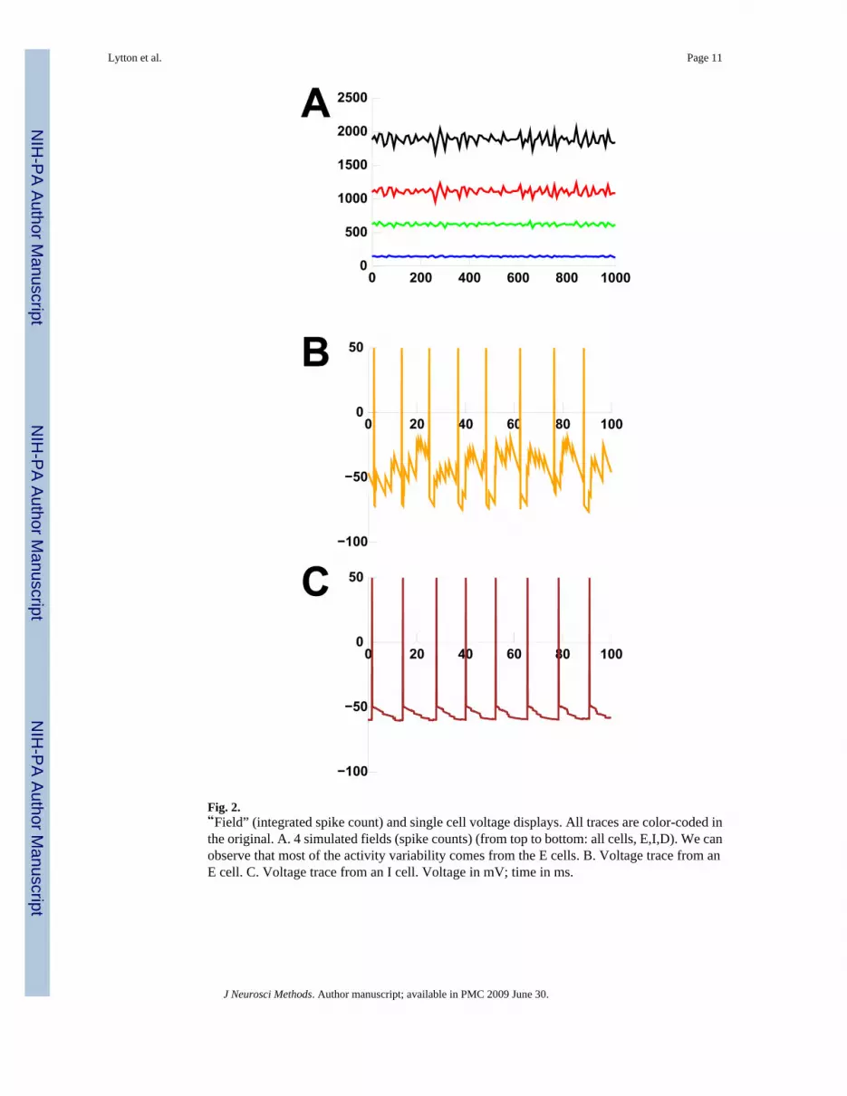
Fig. 2.“Field” (integrated spike count) and single cell voltage displays. All traces are color-coded inthe original. A. 4 simulated fields (spike counts) (from top to bottom: all cells, E,I,D). We canobserve that most of the activity variability comes from the E cells. B. Voltage trace from anE cell. C. Voltage trace from an I cell. Voltage in mV; time in ms.



NIH


NIH


NIH


Fig. 3.Redundant views of the cells in slice permit placement of stimulating and recording electrodes.Top view launches traces such as those of Fig. 2; Middle view is an animation where ellipseheight shows activity in the colored population; Bottom view is a cell-level animation ofvoltages.



NIH


NIH


NIH


Fig. 4.Panel permits saving to a variety of file formats.



NIH


NIH


NIH


Fig. 5.Panel for changing A. weight parameters; B. intrinsic cell parameters for the Expressor cells.



NIH


NIH


NIH


Fig. 6.(A) Instantaneous 35% reduction in E→D cell synaptic strength terminates most randomnetworks (9 out of 10 networks with identical parameters but different randomized connectivityand individual cell properties). Note that activity in top-most trace does not terminate aftersynaptic strength reduction. (B) Wash in (wi) of same parameter change over 300 ms resultsin no termination over 10 other random networks, though activity drops transiently. Detail atbottom shows top trace at 2×. wo is washout period. Baseline for simulation ~1880 spikes/10ms; vertical scalebar 500 spikes/10 ms.



NIH


NIH


NIH


Documents

The virtual slice setup