arX

iv:1

105.

0520

v1 [

astr

o-ph

.CO

] 3

May

201

1Accepted for publication in The Astrophysical JournalPreprint typeset using LATEX style emulateapj v. 11/10/09

THE XMM-NEWTON WIDE FIELD SURVEY IN THE COSMOS FIELD:REDSHIFT EVOLUTION OF AGN BIAS AND SUBDOMINANT ROLE OF MERGERS IN TRIGGERING

MODERATE LUMINOSITY AGN AT REDSHIFT UP TO 2.2

V. Allevato1, A. Finoguenov2,5, N. Cappelluti8,5, T. Miyaji6,7, G. Hasinger1, M. Salvato1,3,4, M. Brusa2, R.Gilli8, G. Zamorani8, F. Shankar14, J. B. James10,11, H. J. McCracken9, A. Bongiorno2, A. Merloni3,2, J. A.

Peacock10, J. Silverman12 and A. Comastri8

Accepted for publication in The Astrophysical Journal

ABSTRACT

We present a study of the redshift evolution of the projected correlation function of 593 X-rayselected AGN with IAB < 23 and spectroscopic redshifts z < 4, extracted from the 0.5-2 keV X-raymosaic of the 2.13deg2 XMM-COSMOS survey. We introduce a method to estimate the average bias ofthe AGN sample and the mass of AGN hosting halos, solving the sample variance using the halo modeland taking into account the growth of the structure over time. We find evidence of a redshift evolutionof the bias factor for the total population of XMM-COSMOS AGN from b(z = 0.92) = 2.30± 0.11 to

b(z = 1.94) = 4.37±0.27 with an average mass of the hosting DM halos logM0[h−1M⊙] ∼ 13.12±0.12

that remains constant at all z < 2.Splitting our sample into broad optical lines AGN (BL), AGN without broad optical lines (NL) andX-ray unobscured and obscured AGN, we observe an increase of the bias with redshift in the range z =0.7− 2.25 and z = 0.6− 1.5 which corresponds to a constant halo mass logM0[h

−1M⊙] ∼ 13.28± 0.07and logM0[h

−1M⊙] ∼ 13.00 ± 0.06 for BL /X-ray unobscured AGN and NL/X-ray obscured AGN,respectively.The theoretical models which assume a quasar phase triggered by major mergers can not reproducethe high bias factors and DM halo masses found for X-ray selected BL AGN with LBOL ∼ 2×1045ergs−1. Our work extends up to z ∼ 2.2 the z . 1 statement that, for moderate luminosity X-ray selectedBL AGN, the contribution from major mergers is outnumbered by other processes, possibly secularsuch as tidal disruptions or disk instabilities.Subject headings: Surveys - Galaxies: active - X-rays: general - Cosmology: Large-scale structure of

Universe - Dark Matter

1. INTRODUCTION

Investigating the clustering properties of active galac-tic nuclei (AGN) is important to put tight constraintson how the AGN are triggered and fueled, to identify

1 Max-Planck-Institut fur Plasmaphysik, Boltzmannstrasse 2,D-85748 Garching, Germany

2 Max-Planck-Institute fur Extraterrestrische Physik, Giessen-bachstrasse 1, D-85748 Garching, Germany

3 Excellent Cluster Universe, Boltzmannstrasse 2, D-85748,Garching, Germany

4 California Institute of Technology, 1201 East CaliforniaBoulevard, Pasadena, 91125, CA

5 University of Maryland, Baltimore County, 1000 Hilltop Cir-cle, Baltimore, MD 21250, USA

6 Instituto de Astronomia, Universidad Nacional Autonomade Mexico, Ensenada, Mexico (mailing adress: PO Box 439027,San Ysidro, CA, 92143-9024, USA)

7 Center for Astrophysics and Space Sciences, University ofCalifornia at San Diego, Code 0424, 9500 Gilman Drive, La Jolla,CA 92093, USA

8 INAF-Osservatorio Astronomico di Bologna, Via Ranzani 1,40127 Bologna, Italy

9 Observatoire de Paris, LERMA, 61 Avenue de l’Obervatoire,75014 Paris, France

10 Astronomy Department, University of California, Berkeley,601 Campbell Hall, Berkeley CA, 94720-7450, USA

11 Dark Cosmology Centre, University of Copenhagen, JulianeMaries Vej 30, 2100 Copenhagen, Denmark

12 Institute for the Physics and Mathematics of the Uni-verse, The University of Tokyo, 5-1-5 Kashiwanoha, Kashiwa-shi, Chiba 277-8583, Japan

14 Max-Planck-Institute fur Astrophysik, Karl-Scwarzschild-Str., D-85748 Garching, Germany

the properties of the AGN host galaxies, and to under-stand how galaxies and AGN co-evolve. In addition, inthe framework of the cold dark matter (CDM) structureformation scenario, clustering properties or the bias ofAGN, may be related to the typical mass of dark mat-ter (DM) halos in which they reside (Mo & White 1996;Sheth & Tormen 1999; Sheth et al. 2001; Tinker et al.2005) and allow various types of AGN to be placed ina cosmological context.Recently, several studies have been made, employ-

ing spectroscopic redshifts to measure the three dimen-sional correlation function of X-ray AGN. The major-ity of the X-ray surveys agree with a picture where X-ray AGN are typically hosted in DM halos with massof the order of 12.5 < logMDM [h−1M⊙] < 13.5, at low(z < 0.4) and high (z ∼ 1) redshift (Gilli et al. 2005;Yang et al. 2006; Gilli et al. 2009; Hickox et al. 2009;Coil et al. 2009; Krumpe et al. 2010; Cappelluti et al.2010). This implies that X-ray AGN more likely residein massive DM halos and preferentially inhabit dense en-vironment typical of galaxy groups.There have been attempts to detect X-ray luminos-

ity dependence of the clustering. At z ∼ 1, neitherGilli et al. (2009) nor Coil et al. (2009) found significantdependence of the clustering amplitudes on the opticalluminosity, X-ray luminosity or hardness ratio, partiallydue to the larger statistical errors. Recent works byKrumpe et al. (2010) and Cappelluti et al. (2010) found,

2 Allevato et al.

however, that high X-ray luminosity AGN cluster morestrongly than low X-ray luminosity ones at 2σ level forz ∼ 0.3 and z ∼ 0, respectively.Until recently, the clustering of AGN has been studied

mainly in optical, particularly in large area surveys suchas 2dF (2QZ, Croom et al. 2005; Porciani & Norberg2006) and Sloan Digital Sky Survey (SDSS, Li et al.2006; Shen et al. 2009; Ross et al. 2009). Croom et al.(2005) analysed the clustering of 2QZ QSO as a func-tion of redshift finding a strong evolution of QSO bias,with bQ(z = 0.53) = 1.13 ± 0.18 at low redshift andbQ(z = 2.48) = 4.24 ± 0.53 at high redshift, as alsoobserved in Porciani & Norberg (2006). The evidenceof an evolution over time of the bias factor for SDSSquasars has been found in Shen et al. (2009), with biasvalues ranging from bQ(z = 0.50) = 1.32 ± 0.17 tobQ(z = 3.17) = 7.76± 1.44. The results from these sur-veys have also shown that the bias evolution of opticallyselected quasars is consistent with an approximately con-stant mass at all redshifts of the hosting DM halo in therange logMDM ∼ 12.5− 13[h−1M⊙].Besides models of major mergers between gas-rich galax-ies appear to naturally produce the bias of quasars asa function of L and z (Hopkins et al. 2008; Shen 2009;Shankar et al. 2009, 2010; Shankar 2010; Bonoli et al.2009), supporting the observations that bright quasarshost galaxies present a preference for merging systems.It is still to be verified if the results from optical surveyscan be extended to the whole AGN population and inparticular to the X-ray selected AGN.In this paper, we concentrate on the study of the bias

evolution with redshift using different X-ray AGN sam-ples and we focus on the estimation of the bias factorand the hosting halo mass using a new method whichproperly account for the sample variance and the strongevolution of the bias with the time.The paper is organized as follows. In section §2 we de-scribe the XMM-COSMOS AGN sample and the AGNsubsets used to estimate the correlation function. In §3we describe the random catalog generated to reproducethe properties of the data sample and the method tomeasure two-point statistic is explained in §4. The re-sults of the AGN auto-correlation based on the standardmethod of the power-law fitting of the signal and usingthe two-halo term are given in §5. In §6 we present ourown method to estimate the AGN bias factor and theDM halos masses in which AGN reside, solving the sam-ple variance and the bias evolution with redshift and in§7 the results. In §8 we present the redshift evolution ofthe bias factor and the corresponding DM halo massesfor the different AGN subsets. We discuss the results inthe context of previous studies in §9 and we conclude in§10. Throughout the paper, all distances are measuredin comoving coordinates and are given in units of Mpch−1, where h = H0/100 km/s. We use a ΛCDM cosmol-ogy with ΩM = 0.3, ΩΛ = 0.7, Ωb = 0.045, σ8 = 0.8.The symbol log signifies a base-10 logarithm.

2. AGN CATALOG

The Cosmic Evolution Survey (COSMOS) is a multi-wavelength observational project over 1.4 × 1.4 deg2 ofequatorial field centred at (RA,DEC)J2000 = (150.1083,2.210), aimed to study AGN, galaxies, large scale struc-ture of the Universe and their co-evolution. The sur-

vey uses multi wavelength imaging from X-ray to radiobands, including HST (Scoville et al. 2007), SUBARU(Taniguchi et al. 2007), Spitzer (Sanders et al. 2007) andGALEX (Zamojski et al. 2007). The central 0.9 deg2

of the COSMOS field has been observed in X-ray withChandra for a total of 1.8 Ms (Elvis et al. 2009). In ad-diction spectroscopic campaigns have been carried outwith VIMOS/VLT and extensive spectroscopic follow-up have been granted with the IMACS/Magellan, MMTand DEIMOS/KeckII projects.XMM-Newton surveyed 2.13 deg2 of the sky in the COS-MOS field in the 0.5-10 keV energy band for a total of∼ 1.55 Ms (Hasinger et al. 2007; Cappelluti et al. 2007,2009) providing an unprecedently large sample of point-like X-ray sources (1822).The XMM-COSMOS catalog has been cross-correlatedwith the optical multiband catalog (Cappelluti et al.2007), the K-band catalog (McCracken et al. 2010),the IRAC catalog (Sanders et al. 2007; Ilbert et al.2010) and the MIPS catalog (Le Floc’h et al. 2009).Brusa et al. (2010) presented the XMM-COSMOS mul-tiwavelength catalog of 1797 X-ray sources with opti-cal/near infrared identification, multiwavelength prop-erties and redshift information (from Lilly et al. 2007,2009; Trump et al. 2007; Adelman-McCarthy et al. 2006;Prescott et al. 2006; Salvato et al. 2009).In this paper we focus on the clustering analysis of

1465 XMM-COSMOS AGN detected in the energy band0.5-2 keV, for which we have a spectroscopic complete-ness of ∼ 53% (780/1465). From this sample of 780objects we selected 593 sources with IAB < 23 (thismagnitude cut increases the spectroscopic completenessto about 65%) and redshift z < 4. The redshift dis-tribution of the AGN sample (Fig. 1 left panel) showsprominent peaks at various redshifts, z ∼ 0.12, z ∼ 0.36,z ∼ 0.73, z ∼ 0.95, z ∼ 1.2, z ∼ 2.1. In particular,the structure at z ∼ 0.36 was also observed at otherwavelengths in COSMOS (Lilly et al. 2007) and alreadydiscussed (Gilli et al. 2009). The median redshift of thesample is < z >= 1.22.The sources have been classified in Brusa et al. (2010)in broad optical line AGN (BL AGN, 354), non-broadoptical line AGN (NL AGN, 239) using a combinationof X-ray and optical criteria, motivated by the fact thatboth obscured and unobscured AGN can be misclassifiedin spectroscopic studies, given that the host galaxy lightmay over shine the nuclear emission. Fig. 2 shows theredshift distribution of BL AGN with < z >= 1.55 andNL AGN with < z >= 0.74.We also studied the clustering properties of X-ray un-obscured and obscured AGN derived on the basis of theobserved X-ray hardness ratio and corrected to take intoaccount the redshifts effects. In particular we used thehard X-ray band (2-10 keV) (which allows us to sam-ple the obscured AGN population) to select a subset of184 X-ray unobscured sources (X-unobs hereafter) withlogNH < 22 cm−2 and 218 X-ray obscured (X-obs here-after) sources with logNH ≥ 22 cm−2, The medianredshift of the two sub-samples are < z >= 1.12 and< z >= 1.30, respectively (see fig. 2, right panel). The47% (40%) of BL (NL) AGN have been also observed inthe hard band and classified as X-unobs (X-obs) AGN.

Redshift Evolution of AGN bias 3

Fig. 1.— Left panel : Redshift distribution of 593 AGN (gold filled histogram) in bins of ∆z = 0.01, with median z = 1.22. The solidblack curve is the Gaussian smoothing of the AGN redshift distribution with σz = 0.3, used to generate the random sample (red emptyhistogram). Right panel : distribution of AGN pairs in redshift bins ∆z = 0.01.

NL AGN (239)Gauss Smoothing

Scaled Random Sample

AGN spec-z (593)NL AGN (239)

BL AGN (354)Gaussian Smoothing

Scaled Random Sample

AGN spec-z (593)BL AGN (354)

X-ray Unobscured (184)Gauss SmoothingScaled Random Sample

X-ray Unobscured (184)

X-ray Obscured (218)Gaussian SmoothingScaled Random Sample

X-ray Obscured (218)

Fig. 2.— Left Panel : Redshift distribution of XMM-COSMOSAGN (open histogram) selected in the soft band, compared with the redshiftdistribution of BL AGN (blue histogram, upper right quadrant) and NL AGN, (red, upper left quadrant). Lower quadrants show the redshiftdistribution of the random catalogs (open black histograms) for both the AGN sub-samples, obtained using a Gaussian smoothing (goldlines) of the redshift distribution of the real samples. Right Panel : Redshift distribution of unobscured (dark blue histogram) and obscured(magenta histogram) AGN selected in the hard band according with the column density (upper quadrants). Lower quadrants show theredshift distribution of the random catalogs (open black histograms) for both the AGN sub-samples, obtained using a Gaussian smoothing(gold lines) of the redshift distribution of the real samples.

3. RANDOM CATALOG

The measurements of two-point correlation functionrequires the construction of a random catalog with thesame selection criteria and observational effects as thedata, to serve as an unclustered distribution to whichto compare. XMM-Newton observations have varyingsensitivity over the COSMOS field. In order to createan AGN random sample, which takes the inhomogeneityof the sensitivity over the field into account, each simu-lated source is placed at random position in the sky, withflux randomly extracted from the catalog of real sources

fluxes (we verified that such flux selection produces thesame results as if extracting the simulated sources froma reference input logN-logS). The simulated source iskept in the random sample if its flux is above the sen-sitivity map value at that position (Miyaji et al. 2007;Cappelluti et al. 2009). Placing these sources at randomposition in the XMM-COSMOS field has the advantageof not removing the contribution to the signal due to an-gular clustering. On the other hand, this procedure doesnot take into account possible positional biases relatedto the optical follow-up program. Gilli et al. (2009), who

4 Allevato et al.

instead decided to extract the coordinates of the randomsources from the coordinate ensemble of the read sam-ple, showed that there is a difference of only 15% in thecorrelation lengths measured with the two procedures.The corresponding redshift for a random object is as-

signed based on the smoothed redshift distribution ofthe AGN sample. As in Gilli et al. (2009) we assumeda Gaussian smoothing length σz = 0.3. This is a goodcompromise between scales that are either too small, thusaffected by local density variations or too large and thusoversmooth the distribution (our results do not changesignificantly using σz = 0.2 − 0.4). Fig. 1 (left panel)shows the redshift distribution of 593 XMM-COSMOSAGN and the scaled random sample (∼ 41000 randomsources) which follows the red solid curve obtained byGaussian smoothing.

4. TWO-POINT STATISTICS

A commonly used technique for measuring the spatialclustering of a class of objects is the two-point correlationfunction ξ(r), which measures the excess probability dPabove a random distribution of finding an object in a vol-ume element dV at a distance r from another randomlychosen object (Peebles 1980):

dP = n[1 + ξ(r)]dV (1)

where n is the mean number density of objects. In par-

Fig. 3.— Projected AGN correlation function wp(rp) computedat different rp scale (see label) as function of the integral radiusπmax. Horizontal lines show that the ACF saturates for πmax >40Mpc/h, which is also the minimum πmax at which wp(rp) convergesand returns the smaller error on the best-fit correlation parameterr0, with γ fixed to 1.8.

ticular, the auto-correlation function (ACF) measuresthe excess probability of finding two objects from thesame sample in a given volume element. With a red-shift survey, we cannot directly measure ξ(r) in physicalspace, because peculiar motions of galaxies distort theline-of-sight distances inferred from redshift. To separatethe effects of redshift distortions, the spatial correlationfunction is measured in two dimensions rp and π, whererp and π are the projected comoving separations be-

tween the considered objects in the directions perpendic-ular and parallel, respectively, to the mean line-of-sightbetween the two sources. Following Davis & Peebles(1983), r1 and r2 are the redshift positions of a pair ofobjects, s is the redshift-space separation (r1 − r2), andl = 1

2 (r1 + r2) is the mean distance to the pair. Theseparations between the two considered objects across rpand π are defined as:

π=s · l

|l|(2)

rp=√

(s · s− π2) (3)

Redshift space distortions only affect the correla-tion function along the line of sight, so we esti-mate the so-called projected correlation function wp(rp)(Davis & Peebles 1983):

wp(rp) = 2

∫ πmax

0

ξ(rp, π)dπ (4)

where ξ(rp, π) is the two-point correlation function interm of rp and π, measured using the Landy & Szalay(1993, LS) estimator:

ξ =1

RR′[DD′ − 2DR′ +RR′] (5)

DD’, DR’ and RR’ are the normalized data-data, data-random and random-random number of pairs definedby:

DD′ =DD(rp, π)

nd(nd − 1)(6)

DR′ =DR(rp, π)

ndnr(7)

RR′ =RR(rp, π)

nr(nr − 1)(8)

where DD, DR and RR are the number of data-data,data-random and random-random pairs at separationrp ± ∆rp and π ± ∆π and nd, nr are the total numberof sources in the data and random sample, respectively.Fig. 1 (right panel) shows the number of pairs in redshiftbins ∆z = 0.01 for the AGN sample.The LS estimator has been used to measure cor-

relations in a number of surveys, for example, SDSS(Zehavi et al. 2005; Li et al. 2006), DEEP2 (Coil et al.2007, 2008), AGES (Hickox et al. 2009), COSMOS(Gilli et al. 2009). If πmax = ∞, then we average overall line-of-sight peculiar velocities, and wp(rp) can be di-rectly related to ξ(r) for a power-law parameterization,by:

wp(rp) = rp

(

r0rp

)γΓ(1/2)Γ[(γ − 1)/2]

Γ(γ/2)(9)

In practice, we truncate the integral at a finite πmax

value, to maximize the correlation signal. One shouldavoid values of πmax too large since they would add noiseto the estimate of wp(rp); if instead, πmax is too smallone would not recover all the signal. To determine theappropriate πmax values for the XMM-COSMOS AGNcorrelation function, we estimated wp(rp) for differentvalues of πmax in the range 20-120 Mpc h−1. Besides, wedetermined the correlation length r0 for this set of πmax

Redshift Evolution of AGN bias 5

Fig. 4.— Left panel : Projected AGN ACF (black circles) compared to the auto-correlation of BL AGN (blue squares) and NL AGN(red triangles). The data points are fitted with a power-law model using the χ2 minimization technique; the errors are computed with abootstrap resampling method. Right panel : The confidence contours of the power-law best-fit parameters r0 and γ, for the whole AGNsample (black), for the BL AGN (blue) and NL AGN (red) sub-samples. The contours mark the 68.3% and 95.4% confidence levels(respectively corresponding to ∆χ2 = 2.3 and 6.17) are plotted as continuous and dotted lines.

values, by fitting wp(rp) with a fixed γ=1.8 over rp in therange 0.5-40 Mpc h−1. In Fig. 3 we show the increase ofthe projected AGN auto-correlation wp(rp) as a functionof the integration radius πmax. The wp(rp) values ap-pear to converge for πmax > 40 Mpc h−1. Therefore weadopt πmax= 40Mpc h−1 in the following analysis, whichis the minimum πmax at which the correlation functionconverges. Such πmax selection returns the smallest erroron the best-fit correlation parameter r0.

5. PROJECTED AUTO-CORRELATION FUNCTION

5.1. Standard Approach

To estimate the AGN auto-correlation function ξ(rp, π)using the LS formula (Eq. 5), we created a grid with rpand π in the range 0.1-100 Mpc h−1, in logarithmic bins∆log(rp, π) = 0.2 and we projected ξ(rp, π) on rp usingEq. 4.In literature, several methods are adopted for error esti-mates in two-point statistics and no one has been provedto be the most precise. It is known that Poisson es-timators generally underestimate the variance becausethey do not account for the fact that the points are notstatistically independent, i.e. the same objects appearin more than one pair. In this work we computed theerrors on wp(rp) with a bootstrap resampling technique(Coil et al. 2009; Hickox et al. 2009; Krumpe et al. 2010;Cappelluti et al. 2010).The standard approach used to evaluate the power of

the clustering signal is to fit wp(rp) with a power-lawmodel (Coil et al. 2009; Hickox et al. 2009; Gilli et al.2009; Krumpe et al. 2010; Cappelluti et al. 2010) of theform given in Eq. 9, using a χ2 minimization technique,with γ and r0 as free parameters. Fig. 4 (left panel, up-per quadrant) shows the projected AGN ACF, evaluatedin the projected separation range rp= 0.5-40 Mpc h−1.The best-fit correlation length and slope and the corre-

sponding 1σ errors, are found to be r0 = 7.12+0.28−0.18 Mpc

h−1 and γ = 1.81+0.04−0.03.

We estimated the projected correlation function of BLand NL AGN in the range rp = 0.5 − 40 Mpc h−1,as shown in Fig.4 (left panel, lower quadrant). For BLAGN we found a correlation length r0 = 7.08+0.30

−0.28 Mpc

h−1 and γ = 1.88+0.04−0.06, while for NL AGN we measured

r0 = 7.12+0.22−0.20 Mpc h−1 and a flatter slope γ = 1.69+0.05

−0.05.Fig. 4 (right panel) shows the power-law best-fit param-eters for the different AGN samples with the 1σ and 2σconfidence intervals for a two parameter fit, which corre-spond to χ2 = χ2

min + 2.3 and χ2 = χ2min + 6.17.

We can estimate the AGN bias factor using the power-law best fit parameters:

bPL = σ8,AGN (z)/σDM (z) (10)

where σ8,AGN (z) is rms fluctuations of the density distri-bution over the sphere with a comoving radius of 8 Mpch−1, σDM (z) is the DM correlation function evaluated at8 Mpc h−1, normalized to a value of σDM (z = 0) = 0.8.For a power-law correlation function this value can becalculated by (Peebles 1980):

(σ8,AGN )2 = J2(γ)(r0

8Mpc/h)γ (11)

where J2(γ) = 72/[(3− γ)(4 − γ)(6 − γ)2γ ]. As the lin-ear regime of the structure formation is verified onlyat large scales, the best-fit parameters r0 and γ areestimated fitting the projected correlation function onrp = 1 − 40 Mpc h−1. The 1σ uncertainty of σ8,AGN iscomputed from the r0 vs. γ confidence contour of thetwo-parameter fit corresponding to χ2 = χ2

min + 2.3.

5.2. Two-halo Term

In the halo model approach, the two-point correlationfunction of AGN is the sum of two contributions: the

6 Allevato et al.

TABLE 1Bias Factors and hosting DM halo masses

(1) (2) (3) (4) (5)AGN < z >a bPL b2−h logMDM

b

Sample Eq. 10 Eq. 16 h−1M⊙

Total (593) 1.22 2.80+0.22−0.90 2.98± 0.13 13.23 ± 0.06

BL (354) 1.55 3.11+0.30−1.22 3.43± 0.17 13.14 ± 0.07

NL (239) 0.74 2.78+0.45−1.07 2.70± 0.22 13.54 ± 0.10

X-unobs (184) 1.12 2.98+0.34−0.37 3.01± 0.21 13.33 ± 0.08

X-obs (218) 1.30 1.66+0.31−0.32 1.80± 0.15 12.30 ± 0.15

Subsample at z < 1BL (70) 0.57 2.18+0.95

−1.02 2.32± 0.26 13.50 ± 0.11

NL (137) 0.53 1.68+0.45−0.57 1.40± 0.15 12.65 ± 0.18

a Median redshift of the sample.b Typical DM halo masses based on Sheth et al. (2001) andvan den Bosch (2002).

Fig. 5.— Factor g as defined in Eq. 21, estimated at the redshiftof each AGN (black triangles). The data points are fitted by thefunction D1(z)/D1(z = 0), where D1(z) is the growth function (seeEq. (10) in Eisenstein & Hu 1999 and references therein). The biasof each AGN is weighted by this factor according to the redshift zof the source.

first term (1-halo term) is due to the correlation betweenobjects in the same halo and the second term (2-haloterm) arises because of the correlation between two dis-tinct halos:

wAGN (rp) = w1−hAGN (rp) + w2−h

AGN (rp) (12)

As the 2-halo term dominates at large scales, we can con-sider this term to be in the regime of linear density fluc-tuations. In the linear regime, AGN are biased tracersof the DM distribution and the AGN bias factor definesthe relation between the two-halo term of DM and AGN.

w2−hAGN (rp) = b2AGNw2−h

DM (rp) (13)

We first estimated the DM 2-halo term at the medianredshift of the sample, using:

ξ2−hDM (r) =

1

2π2

∫

P 2−h(k)k2[

sin(kr)

kr

]

dk (14)

Fig. 6.— Projected AGN ACF (black circles) compared to

b2w2−h

DM(rp, z = 0) (dotted line), where the weighed bias b is de-

fined in Eq. 22. The shaded region shows the projected DM 2-haloterm scaled by (b ± δb)2.

where P 2−h(k) is the Fourier Transform of the linearpower spectrum, assuming a power spectrum shape pa-rameter Γ = 0.2 and h = 0.7. Following Hamana et al.(2002), we estimated ξ2−h

DM (r) and then the DM projected

correlation w2−hDM (rp) using:

w2−hDM (rp) = 2

∫ ∞

rp

ξ2−hDM (r)rdr√

r2 − r2p

(15)

Using this term, we can estimate the AGN bias simplydividing the projected AGN correlation function at largescale (rp > 1 Mpc h−1) by the DM 2-halo term:

b2AGN = (wAGN2− h(rp)/w2−hDM (rp))

1/2 (16)

and then averaging over the scales rp = 1− 40 Mpc h−1.Table 1, column 4 shows the AGN bias factors using thismethod, compared with the ones based on the power-lawfits of the ACF (column 3) for the different AGN subsets.The two sets of bias values from the different approachesare consistent within 1σ, but the errors on bPL are biggerconsistently with the fact that the AGN ACF is not welldescribed by a power-law.

6. SOLVING FOR SAMPLE VARIANCE USING HOD

The standard approaches used in previous works onclustering of X-ray AGN (Mullis et al 2004; Yang et al.2006; Gilli et al. 2005; Coil et al. 2009; Hickox et al.2009; Krumpe et al. 2010; Cappelluti et al. 2010) to es-timate the bias factors from the projected AGN ACF arebased on the power-law fit parameters (method 1). Thismethod assumes that the projected correlation functionis well fitted by a power-law and the bias factors arederived from the best fit parameters r0 and γ of the clus-tering signal at large scale.Most of the authors (Hickox et al. 2009; Krumpe et al.2010; Cappelluti et al. 2010) used an analytical expres-sion (as the one described in Sheth & Tormen 1999;

Redshift Evolution of AGN bias 7

Fig. 7.— Projected ACF of BL AGN (blue triangles, left panel) and NL AGN (red squares, right panel), compared to b2w2−h

DM(rp, z = 0)

(dotted line), where the weighed bias b is defined in Eq. 22. The shaded region shows the projected DM 2-halo term scaled by (b ± δb)2.

Fig. 8.— Projected ACF of X-unobs AGN (darkblue open circles, left panel) and X-obs AGN (magenta diagonal crosses, right panel),

compared to b2w2−h

DM(rp, z = 0) (dotted line), where the weighed bias b is defined in Eq. 22. The shaded region shows the projected DM

2-halo term scaled by (b ± δb)2.

Sheth et al. 2001; Tinker et al. 2005) to assign a char-acteristic DM halo mass to the hosting halos. The in-congruity of this approach is that the bias used is theaverage bias of a given sample at a given redshift. How-ever, the average bias is sensitive to the entirety of themass distribution so that distributions with different av-erage masses, can give rise to the same average bias value.In the halo model approach the large scale amplitude sig-nal is due to the correlation between objects in distincthalos and the bias parameter defines the relation betweenthe large scale clustering amplitude of the AGN ACF andthe DM 2-halo term (method 2).In literature, the common model used for the AGN

HOD is a three parameter model including a step func-

tion for the HOD of central AGN and a truncated power-law satellite HOD (introduced by Zehavi et al. 2005, forgalaxies). Here we assumed that all the AGN residein central galaxies. This assumption is supported byStarikova et al. (2010). They found that X-ray AGN arepredominantly located in the central galaxies of the hostDM halos and tend to avoid satellite galaxies, fixing thelimit to the fraction of AGN in non-central galaxies tobe less than 10%. The same fraction of satellites galaxieshosting AGN is suggested in Shen (2009). Shankar et al.(2010) modelled the measurements of quasar clusteringderived in the SDSS (Shen et al. 2009) and they verifiedthat the predicted bias factors and the correlation func-tions are not altered including subhalos as quasar hosts.

8 Allevato et al.

TABLE 2Weighted Bias factors and hosting DM halo masses

(1) (2) (3) (4) (5)AGN b z logM0 bS01

a

Sample Eq. 22 Eq. 23 h−1M⊙

Total (593) 1.91± 0.13 1.21 13.10± 0.06 2.71± 0.14BL (354) 1.74± 0.17 1.53 13.24± 0.06 3.68± 0.27NL (239) 1.80± 0.22 0.82 13.01± 0.08 2.00± 0.12X-unobs (184) 1.95± 0.21 1.16 13.30± 0.10 3.01± 0.26X-obs (218) 1.37± 0.15 1.02 12.97± 0.08 2.23± 0.13

Subsample at z < 1BL (70) 1.62± 0.26 0.63 13.27± 0.10 1.95± 0.17NL (137) 1.56± 0.15 0.60 12.97± 0.07 1.62± 0.15

a Bias estimated from M0 using Sheth et al. (2001).

A further consideration is that there is in practice no dis-tinction between central and satellite AGN in the 2-haloterm that we used to estimate the AGN bias factor.We assumed a simple parametric form of the AGN halo

occupation NA, described by a delta function:

NA(MDM ) = fAδ(MDM −M0) (17)

where fA is the AGN duty cycle. It is clear that we arenot considering the full HOD model, but we are assigningto all the AGN the same average mass of the hostinghalos. The motivation is that X-ray AGN mainly residein massive halos with a narrow distribution of the hostinghalo masses. It’s clear that this assumption is specific toAGN and e.g. is not applicable to galaxies.The AGN HOD descrived by δ-function is motivated by

the results of Miyaji et al. (2011) showing that the AGNHOD rapidly decreases at high halo masses. In additionMartini et al. (2009) and Silverman et al. (2009) foundthat AGN preferentially reside in galaxy groups ratherthan in clusters.The δ-function is the simplest possible assumption in thetreatment of the sample variance, which is due to thevariation in the amplitude of source counts distribution.It has been shown in Faltenbacher et al. (2010), that thevariation in the density field, which is responsible for thesample variance, can be replaced by the variation of thehalo mass function. In terms of halo model, the biasfactor as a function of the fluctuations ∆ in the densityfield is expressed by:

bA(∆) =

∫

MhNA(Mh)bh(Mh)nh(Mh,∆)dMh∫

MhNA(Mh)nh(Mh,∆)dMh

(18)

where NA is the AGN HOD, bh(MDM ) is the halo biasand nh(MDM ,∆) is the halo mass function, which de-pends on the density field. On the other hand the sam-ple variance does not effect the AGN halo occupation. InAllevato et al. (in prep.) we confirm the assumption ofconstancy of the AGN HOD with the density field.When we assume that all AGN reside in DM halos withthe same mass, Eq. 18 becomes simpler:∫

Mhδ(Mh −M0)bh(Mh)nh(Mh,∆)dMh∫

Mhδ(Mh −M0)nh(Mh,∆)dMh

= b(M0) (19)

The equation shows that when the AGN HOD is closeto a δ-function, the variations in the density field only

change the AGN number density and put more weight onAGN bias at the redshift of large scale structure (LSS),but do not change the bias of AGN inside the structure.Our claim differs from the results presented in Gilli et al.(2005) and (Gilli et al. 2009). They found that excludingsources located within a large-scale structures, the corre-lation length and then the bias factor strongly reduces.Such bias behaviour can be used to constrain more com-plicated shapes of the AGN HOD than a δ-function typedistribution.However, even in the case of a δ-function HOD, we still

need to consider the two effects which are often omittedin the clustering analysis: the LSS growth and the evolu-tion of the bias factor with z. Ignoring these effects canby itself lead to a difference in the results reported forthe different AGN samples.The bias factor depends on the redshift as the struc-

tures grow over time, associated with our use of a largeredshift interval. For the ith source at redshift zi, weconsidered the bias factor corresponding to a halo massMDM = M0:

bi = b(M0, zi) (20)

where b(M0, z) is evaluated using van den Bosch (2002)and Sheth et al. (2001). For each AGN at redshift z weestimated the factor g(z) defined as the square root ofthe projected DM 2-halo term at redshift z normalizedto the projected DM 2-halo term evaluated at z = 0:

g(z) =

√

wDM (z, rp)

wDM (z = 0, rp)(21)

averaged over the scales rp = 1 − 40 Mpc h−1. As theamplitude of the projected DM 2-halo term decreaseswith increasing redshift, g is a decreasing function of z(see fig. 5), well described by the term D1(z)/D1(z =0), where D1(z) is the growth function (see eq. (10) inEisenstein & Hu (2001) and references therein).By accounting for the fact that the linear regime of thestructure formation is verified only at large scales, weestimated the AGN bias considering only the pairs whichcontribute to the AGN clustering signal at rp = 1 − 40Mpc h−1. We defined the weighted bias factor of thesample as:

b(M0) =

√

∑

i,j bibjgigj

Npair(22)

where bibj is the bias factor of the ith and jth source inthe pair i− j, gigj is the g factor of the pair and Npair isthe total number of pairs in the range rp = 1 − 40 Mpch−1.Similarly, we defined a weighted average redshift of theAGN sample, weighting the redshift of each pair for theg factor and the bias of the pair (bibj):

z =

∑

i,j bibjgigjzpair∑

i,j bibjgigj(23)

where zpair = (zi + zj)/2. Following this approach wecan find the value of M0 that satisfies:

b1 = b(M0)

Redshift Evolution of AGN bias 9

where b1 is the square root of the projected AGN ACFnormalized to the projected DM 2-halo term at z = 0:

b1 =

√

wAGN (rp)

wDM (z = 0, rp)(24)

averaged over the scale rp = 1− 40 Mpc h−1.By performing the test in narrow redshift intervals, we

can study the dependency of the halo mass M0 on red-shift (see §8). Moreover with just a single measurementof the amplitude of the 2-halo term, one cannot constrainthe AGN HOD. Already with several measurements sam-pling different density fields, the shape of the HOD canbe linked to the LSS density-dependence of the bias. Inaddition, the 1-halo term of the AGN auto-correlationand AGN-groups cross-correlation can be used to dis-criminate between different HOD models, which will beargument of our following work.

7. MEASUREMENTS

The weighted bias factors b and redshifts z, and thecorresponding DM halo masses M0 estimated for the dif-ferent AGN sub-samples using the method described inthe previous section are shown in Table 2.Fig. 6, 7 and 8 show the ACF of the AGN, BL/NL AGNand X-unobs/obs AGN samples, compared to the term

b2w2−h

DM (rp, z = 0) (dotted line), where the weighed bias

b is defined in Eq. 22. The shaded region shows theprojected DM 2-halo term scaled by (b± δb)2.The AGN bias factor indicates that XMM-COSMOS

AGN reside in halos with average mass logM0 = 13.01±0.09[h−1logM⊙], characteristic of moderate-size poorgroups, a result consistent with previous works on X-ray selected AGN that indicate that the typical DM halomass hosting AGN is in the range 12.5 . logMDM .13.5[h−1M⊙].We found that BL and NL AGN which peak at z = 1.53and z = 0.82, present consistent bias factors which cor-respond to DM halo average masses logM0 = 13.24 ±0.06[h−1M⊙] and 13.01± 0.08[h−1M⊙], respectively. Asdescribed in Brusa et al. (2010), only a small fraction ofthe objects classified as NL AGN are located at z > 1, tobe compared with 350 in the BL AGN sample. This ismostly due to the fact that high-redshift NL AGN are op-tically faint (typically I ∼ 23−24) and have not been tar-geted yet with dedicated spectroscopic campaigns. Ourresults might be affected by the limitations in the ob-scured AGN classification, considering that some modelson the evolution of the obscured AGN fraction predict anincrease of the fraction with the redshift (Hasinger et al.2008). In order to avoid the problem of different red-shift distribution in comparing BL/NL AGN cluster-ing amplitude, we selected for each sample a subset(BL AGN with 70 sources and NL AGN with 137) atz ∼ 0.6. At the same redshift we found that BL and NLAGN have a bias factor bBL = 1.62 ± 0.26 and bNL =1.56 ± 0.15, which correspond to average halo masseslogM0 = 13.27± 0.10[h−1M⊙] and 12.97± 0.07[h−1M⊙],respectively.Similar results have been obtained using X-unobs and X-obs AGN samples; unobscured AGN at z = 1.16 inhabithalos with average mass logM0 = 13.30 ± 0.10[h−1M⊙]which is higher at 2.5 σ level than the halo mass hosting

obscured AGN (logM0 = 12.97± 0.08[h−1M⊙]), at sim-ilar redshift.In order to compare our results with previous works onthe bias of X-ray selected AGN, we evaluated the biasfactors corresponding to the halo mass M0 at z usingSheth et al. (2001) as shown in Table 2, col (5).Our results support the picture that at a given redshift,

X-ray selected BL/X-unobs AGN reside in more massivehalos compared to X-ray selected NL/X-obs AGN. Thisresult would be expected if the two classes of AGN corre-spond to different phases of the AGN evolution sequence(Hopkins et al. 2006, 2008; Hickox et al. 2009).

8. BIAS EVOLUTION AND CONSTANT MASSTHRESHOLD

In order to investigate the redshift evolution of thebias factor, we split the XMM-COSMOS AGN sample inthree redshift bins. The sizes of the redshift bins havebeen determined such that there are more or less thesame number of objects in each bin. The values of b, zand M0 for the total AGN sample are shown in Table3. The meaning of the table columns are: (1) sample;(2) number of sources; (3) bias parameter from the pro-jected DM 2-halo term, evaluated at the median < z >of the sample; (4) typical halo mass using van den Bosch(2002) and Sheth et al. (2001); (5) weighted bias of thesample; (6) weighted redshift of the sample; (7) AverageDM halo mass; (8) Bias factor from M0 estimated usingSheth et al. (2001).We observed an increase of the AGN bias factor withredshift, from b(z = 0.92) = 1.80 ± 0.19 to b(z =1.94) = 2.63 ± 0.21 with a DM halo mass consistentwith being constant at logM0[h

−1M⊙] ∼ 13.1 in eachbin. These results support the picture that the bias ofXMM-COSMOS AGN evolves with time according to aconstant halo mass track at all redshifts z < 2.This conclusion, based on the analysis of the global

XMM-COSMOS AGN sample, can however be affectedby the fact that the relative proportions of BL and NLAGN are a strong function of redshift. In fact, since theXMM-COSMOS AGN sample is a flux limited sample,more luminous AGN are selected at high redshift and,also because of our magnitude limit, high-z sources inour sample are mainly BL AGN (see §2). For this rea-son BL AGN sample could be analysed up to z ∼ 2.25,while the maximum average redshift of the two redshiftbins for NL AGN is z ∼ 0.91. We found evidence of astrong increase of the BL AGN bias factor in four red-shift bins (see Table 3), with a DM halo mass constantat logM0[h

−1M⊙] ∼ 13.28 at all redshifts z < 2.25. ForNL AGN we estimated b(z = 0.62) = 1.59 ± 0.13 andb(z = 0.91) = 1.87±0.19, which correspond to a constanthalo mass values logM0[h

−1M⊙] ∼ 13.02. We split theX-unobs and X-obs AGN samples in two redshift binsup to z ≃ 1.5 and we found that the bias of X-unobsAGN (X-obs AGN) evolves according to a constant halomass consistent with the mass of BL AGN (NL AGN)hosting halos. Fig. 9 (left panel) shows the redshift evo-lution of the average DM halo mass M0 for all the AGNsubsets. The horizontal lines represent the mean valueof M0 for BL/X-unobs AGN (dashed-blue), NL/X-obsAGN (long dashed-red) and for the whole AGN sample(dotted-black). Fig. 9 (right panel) shows the redshift

10 Allevato et al.

Fig. 9.— Left Panel : DM halo mass M0 as a function of z for different AGN sub-samples (see legend). The horizontal lines show themean value of M0 for BL/X-unobs AGN (dashed-blue), NL/X-obs AGN (long dashed-red) and for the whole AGN sample (dotted-black).Right Panel : Redshift evolution of the bias parameter bS01 of different AGN sub-samples. The dashed lines show the expected b(z) oftypical DM halo masses MDM based on Sheth et al. (2001). The masses are given in logMDM in units of h−1M⊙. BL/X-unobs AGNpresent a strong bias evolution with redshift with a constant DM halo mass logM0 = 13.28± 0.07[h−1M⊙] up to z ∼ 2.4. NL/X-obs AGNreside in less massive halos with logM0 = 13.00 ± 0.06[h−1M⊙], constant at z < 1.5.

TABLE 3Bias Evolution

(1) (2) (3) (4) (5) (6) (7) (8)< z >a

N b2−h logMDMb b z logM0 bS01

c

Eq. 16 h−1M⊙ Eq. 16 h−1M⊙

All AGN0.80 190 2.70± 0.19 13.48 ± 0.10 1.80± 0.19 0.92 13.12 ± 0.06 2.30± 0.111.30 220 3.10± 0.18 13.21 ± 0.10 2.14± 0.18 1.42 13.07 ± 0.08 3.02± 0.112.07 183 5.18± 0.21 13.30 ± 0.11 2.63± 0.21 1.94 13.18 ± 0.08 4.37± 0.27

BL AGN0.67 70 2.62± 0.20 13.57 ± 0.10 1.52± 0.20 0.70 13.26 ± 0.06 2.16± 0.251.25 108 3.06± 0.23 13.24 ± 0.08 2.02± 0.23 1.25 13.21 ± 0.08 3.00± 0.271.71 92 5.37± 0.28 13.60 ± 0.08 3.57± 0.28 1.72 13.32 ± 0.08 4.31± 0.302.46 85 6.82± 0.27 13.41 ± 0.10 4.02± 0.27 2.25 13.28 ± 0.10 5.60± 0.42

X-unobscured AGN0.65 98 2.46± 0.17 13.51 ± 0.11 1.62± 0.17 0.80 13.28 ± 0.05 2.34± 0.181.66 86 4.85± 0.18 13.51 ± 0.10 2.10± 0.18 1.54 13.33 ± 0.06 3.90± 0.33

NL AGN0.53 137 1.40± 0.13 12.65 ± 0.12 1.59± 0.13 0.62 13.01 ± 0.05 1.70± 0.101.02 102 2.11± 0.19 12.88 ± 0.15 1.87± 0.19 0.91 13.04 ± 0.07 2.20± 0.17

X-obscured AGN0.73 106 1.80± 0.14 13.01 ± 0.11 1.51± 0.14 0.85 13.03 ± 0.06 2.08± 0.121.84 112 3.51± 0.16 12.94 ± 0.13 1.96± 0.16 1.51 12.95 ± 0.06 2.95± 0.14

a Median redshift of the sample.b Typical DM halo masses based on Sheth et al. (2001) and van den Bosch (2002).c Bias estimated from M0 using Sheth et al. (2001).

evolution of the bias factors bS01 (Table 3, col (7)) fordifferent AGN sub-samples. The dashed lines show theexpected b(z) associated to the typical DM halo massbased on Sheth et al. (2001).These results show that X-ray selected BL/X-unobsAGN reside in more massive DM halos compared to X-ray selected NL/X-obs AGN at all redshifts z at ∼ 3σlevel. This suggests that the AGN activity is a masstriggered phenomenon and that different AGN phasesare associated with the DM halo mass, irrespective of

redshift z.

9. DISCUSSION

9.1. Which DM halos host X-ray AGN?

We have introduced a new method that uses the 2-haloterm in estimating the AGN bias factor and that prop-erly accounts for the sample variance and the growthof the structures over time associated with our use oflarge redshift interval of the AGN sample. Using this ap-proach we have estimated an average mass of the XMM-

Redshift Evolution of AGN bias 11

0 10

1

2

3

4

5

6

7

8

Fig. 10.— Bias parameter as a function of redshift for various X-ray selected AGN (black data points), X-ray selected BL/X-unobs AGN(blue data points) and X-ray selected NL/X-obs AGN (red data points) as estimated in previous studies and in this work according to thelegend. Our results refer to the bias factor bS01 showed in Table 2 col (5). The dashed lines show the expected b(z) of typical DM halomasses MDM based on Sheth et al. (2001). The masses are given in logMDM in units of h−1M⊙.

COSMOS AGN hosting halos equal to logM0[h−1Mpc] =

13.10 ± 0.06 which differs at ∼ 1.6σ level from the typ-ical halo mass MDM based on Sheth et al. (2001) usingthe methode 2 (see §5.2). The difference between thestandard method and our own method is also clear forthe mass of BL and NL AGN hosting halos. We havefound that BL AGN inhabit DM halos with average masslogM0[h

−1Mpc] = 13.24 ± 0.06 at z = 1.53 while haloshosting NL AGN have average mass logM0[h

−1Mpc] =13.01 ± 0.08. BL AGN reside in more massive halosthan NL AGN also selecting two subsamples that peakat the same median redshift z ∼ 0.6. We obtained simi-lar results using X-ray unobscured AGN at z = 1.16 andX-ray obscured AGN at z = 1.02 (logM0[h

−1Mpc] =13.30± 0.10 and logM0[h

−1Mpc] = 12.97± 0.08, respec-tively).Instead the typical halo mass based on Sheth et al.

(2001) using the AGN bias estimated with the method 2,strongly depends on the median redshift of the sample.According to the method 2, BL AGN at < z >= 1.55reside in less massive halos compared to NL AGN at< z >= 0.74, while the result is different selecting twosamples of BL and NL AGN at the same < z >∼ 0.5.Our results agrees with the majority of the recent studiesof X-ray surveys which suggest a picture in which X-rayAGN are typically hosted in DM halos with mass in therange 12.5 < logMDM [h−1Mpc] < 13.5, at low (< 0.4)and high (∼ 1) redshift. Starikova et al. (2010) foundthat Chandra/Bootes AGN are located at the center ofDM halos with M > Mmin = 4 × 1012 h−1 M⊙. Thismass estimate represents a threshold value, since theyare assuming a halo occupation described by a step func-tion (zero AGN per halo/subhalo below Mmin and oneabove it). Our approach, in terms of HOD, is completely

12 Allevato et al.

0 1 2 3 4

1

2

3

4

5

6

7

8

Fig. 11.— Bias parameter as a function of redshift for optically selected BL AGN from previous works (Croom et al. 2005), green-crosses;Porciani & Norberg (2006), green-stars; Shen et al. (2009), green-open squares; Ross et al. (2009), gree-open triangle) and X-ray selectedBL (blue triangles) and X-unobs (blue open-circles) AGN and NL (red squares) and X-obs (red crosses) AGN as estimated in this work.The dashed lines show the expected b(z) of typical DM halo masses based on Sheth et al. (2001) and the dotted lines represent the passiveevolution of the bias, as described in Fry et al. (1996). The bias of optically selected BL AGN evolves with redshift following an evolutionat constant halo mass, with a typical mass which remains practically in the range logMDM ∼ 12.5 − 13h−1M⊙ at all redshifts z < 2.25.X-ray selected BL/X-unobs AGN reside in more massive DM halos at all redshifts z < 2.25, according to a typical mass of the hostinghalos constant over time in the range logMDM ∼ 13 − 13.5h−1M⊙. The bias evolution of NL/X-obs AGN seems to indicate that theyreside in DM halo mass logMDM ∼ 13h−1M⊙ constant at all z < 1.5. These results suggest the picture that X-ray selected BL AGN aretriggered by secular processes as tidal disruption or disk instabilities instead of major mergers between gas-rich galaxies as confirmed bysemi-analytic models and observations for optically selected quasars.

different. We assume a halo occupation described by δ-function, supported by the fact that AGN only reside inmassive halos (then the AGN HOD can be described bya narrow halo mass distribution at high mass values, butnot by a step function).Fig. 10 shows the bias factors of X-ray selected AGN(black), BL/X-unobs AGN (blue) and NL/X-obs AGN(red) as estimated in different surveys (according to thelegend). Our results refer to the bias factors bS01 showedin Table 2, column (5). The dashed lines show the ex-pected b(z) assuming a constant typical DM halo massMDM , based on Sheth et al. (2001).

The previous studies of Gilli et al. (2005) forthe CDFN, Gilli et al. (2009), Mullis et al (2004),Yang et al. (2006) for CLASXS AGN suggest the sce-nario in which the typical DM halo mass hosting X-ray selected AGN is logMDM [h−1M⊙] ∼ 13.5. Thebias values measured in Gilli et al. (2005) on CDFS, inHickox et al. (2009), Coil et al. (2009) and Yang et al.(2006) and in this work, correspond to a lower halo mass(logMDM [h−1M⊙] ∼ 13). A possible explanation couldbe that at fixed redshift, the bias and then the mass of thehosting halo, depends on the luminosity of the sample.The same explanation might be applied to the results on

Redshift Evolution of AGN bias 13

BL/X-unobs AGN.The bias estimates at z < 1 for NL/X-obs AGN inCappelluti et al. (2010) and in this work, seem to in-dicate that the mass of NL/X-obs AGN hosting halos islogMDM [h−1M⊙] ∼ 13.

9.2. Optically selected vs X-ray selected AGN

We first found evidence of a redshift evolution of thebias factor of X-ray selected BL/ X-unobs AGN (fig. 11,blue data points) and NL/X-obs AGN (red data points).The bias evolves with redshift at constant average halomass logM0[h

−1M⊙] ∼ 13.3 for BL/X-unobs AGN andlogM0[h

−1M⊙] ∼ 13 for NL/X-obs AGN at z < 2.25and z < 1.5, respectively. Fig. 11 shows the expectedb(z) assuming a constant typical DM halo mass basedon Sheth et al. (2001) (dashed lines) and the so calledpassive bias evolution (dotted lines Fry et al. 1996). Theobserved bias evolution suggests an average halo massof the hosting halos, constant over time in the rangelogMDM [h−1M⊙] = 13 − 13.5, instead of an evolutionof the bias in a model in which objects are formed at afixed time and their distribution evolves under the influ-ence of gravity.There have been several studies of the bias evolution of

optical quasar with the redshift as shown in fig. 11 (greendata points), based on large survey samples such as 2QZand SDSS (Croom et al. 2005; Porciani & Norberg 2006;Shen et al. 2009; Ross et al. 2009). Since the quasarsamples used in these clustering analysis are definedas spectroscopically identified quasars with at least onebroad (FWHM>1000 km s−1) emission line, we refers tothem as optically selected BL AGN.All the previous studies infer the picture that the

quasar bias evolves with redshift following a constantmass evolution, with the average mass that can vary inthe range logMDM [h−1M⊙] ∼ 12.5−13, may be depend-ing on the AGN sample luminosity as already suggestedfor X-ray selected AGN. The simplest interpretation ac-cording to the observed redshift evolution of the bias fac-tors is that 1) X-ray selected AGN whether BL/X-unobsor NL/X-obs AGN inhabit DM halos with mass higherthan the mass of optically selected quasar hosting halosin the range z = 0.5−2.25; 2) X-ray selected BL/X-unobsAGN reside in more massive halos compared to NL/X-obs AGN for z = 0.6− 1.6 and the discrepancy betweenthe bias factors of the two samples increases with z; 3)the AGN activity is a mass triggered phenomena and thedifferent AGN evolutionary phases are associated withjust the DM halo mass, irrespective of the redshift z.

9.3. External vs Internal Triggering

The major merger of galaxies is one of the promis-ing mechanisms suggested to be responsible for fuellingquasars and in particular to be dominant for brightquasars at high redshift. Models of major mergers ap-pear to naturally produce many observed properties ofquasars, as the quasar luminosity density, the shapeand the evolution of the quasar luminosity function andthe large-scale quasar clustering as a function of L andz (Hopkins et al. 2008; Shen 2009; Shankar et al. 2009,2010; Shankar 2010; Bonoli et al. 2009).Clear evidence for higher incidence of mergers is seenamong quasars (Serber et al. 2006; Hopkins et al. 2006;

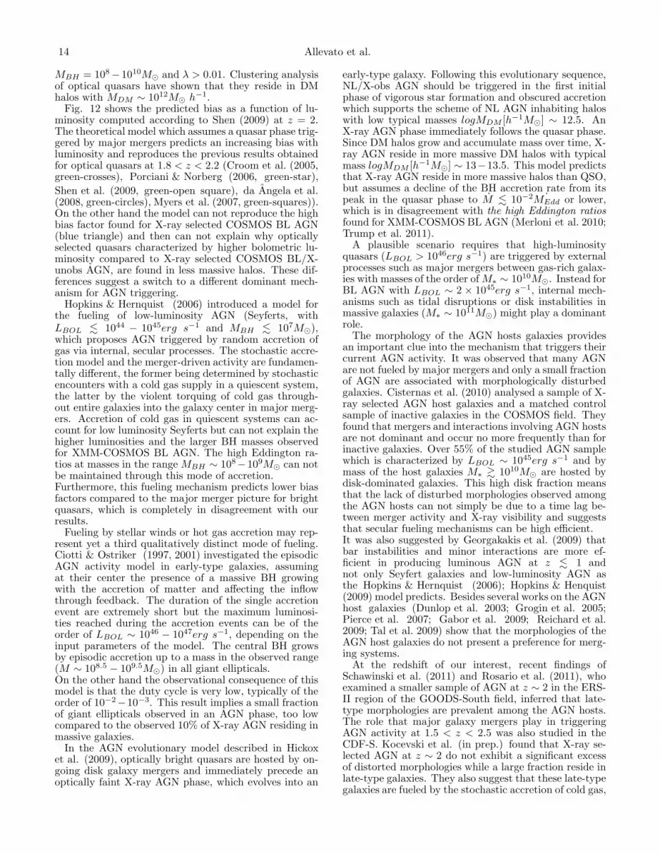
Fig. 12.— Predicted bias as a function of luminosity, computedaccording to Shen (2009) fixing z = 2, compared to previousbias estimates at 1.8 < z < 2.2, for optically selected BL AGNand for XMM-COSMOS BL AGN. Points are measurements fromCroom et al. (2005, green-crosses), Porciani & Norberg (2006,

green-star), Shen et al. (2009, green-open square), da Angela et al.(2008, green-circles), Myers et al. (2007, green-squares) and our re-sult (blue triangle). For ease of comparison, all luminosities areconverted to bolometric luminosities using the corrections fromHopkins et al. (2007). The theoretical model which assumes aquasar phase triggered by major merger reproduces the results ob-tained for the bias of quasars, but can not reproduce the high biasfactors found for X-ray selected BL AGN and then can not explainwhy optically selected quasars that have higher bolometric lumi-nosity compared to COSMOS X-ray selected BL/X-unobs AGN,reside in more massive halos. These differences suggest a switchto a different dominant mechanism for AGN triggering, from ma-jor mergers between gas-rich galaxies to secular processes as tidaldisruptions or disk instabilities.

Veilleux et al. 2009). Additionally a large fraction of lu-minous quasars at low redshift are associated with eithermorphologically disturbed objects (Canalizo & Stockton2001; Guyon et al. 2006), or early-type hosts with finestructure in their optical light distribution, indicativeof past interactions (Canalizo et al. 2007; Bennert et al.2008). In the local Universe, for instance, the studyof the environment of Swift BAT Seyfert galaxies(Koss et al. 2010) appeared to show an apparent mergers∼ 25% which suggests that AGN activity and mergingare critically linked. Moreover it is believed that majormerger dominates at high redshift and bright luminosi-ties (Hasinger et al. 2008; Hopkins et al. 2006), while mi-nor interaction or bar instabilities or minor tidal disrup-tions are important at low redshift (z . 1) and low lu-minosities (LBOL . 1044erg s−1) (Hopkins & Henquist2009).Our results on the bias evolution of X-ray selected

BL/X-unobs AGN infer that these objects with LBOL ∼2 × 1045erg s−1 reside in massive DM halos MDM ∼2 × 1013M⊙h

−1. Besides studies on BL AGN in theCOSMOS field (Merloni et al. 2010; Trump et al. 2011)suggest that our sample is characterized by BH massesin the range MBH = 107 − 109M⊙ and Eddington ra-tio λ > 0.01. Optically selected quasars from large sur-vey samples such as 2QZ and SDSS are high-luminosityquasars LBOL & 1046erg−1 with BH masses in the range

14 Allevato et al.

MBH = 108− 1010M⊙ and λ > 0.01. Clustering analysisof optical quasars have shown that they reside in DMhalos with MDM ∼ 1012M⊙ h−1.Fig. 12 shows the predicted bias as a function of lu-

minosity computed according to Shen (2009) at z = 2.The theoretical model which assumes a quasar phase trig-gered by major mergers predicts an increasing bias withluminosity and reproduces the previous results obtainedfor optical quasars at 1.8 < z < 2.2 (Croom et al. (2005,green-crosses), Porciani & Norberg (2006, green-star),

Shen et al. (2009, green-open square), da Angela et al.(2008, green-circles), Myers et al. (2007, green-squares)).On the other hand the model can not reproduce the highbias factor found for X-ray selected COSMOS BL AGN(blue triangle) and then can not explain why opticallyselected quasars characterized by higher bolometric lu-minosity compared to X-ray selected COSMOS BL/X-unobs AGN, are found in less massive halos. These dif-ferences suggest a switch to a different dominant mech-anism for AGN triggering.Hopkins & Hernquist (2006) introduced a model for

the fueling of low-luminosity AGN (Seyferts, withLBOL . 1044 − 1045erg s−1 and MBH . 107M⊙),which proposes AGN triggered by random accretion ofgas via internal, secular processes. The stochastic accre-tion model and the merger-driven activity are fundamen-tally different, the former being determined by stochasticencounters with a cold gas supply in a quiescent system,the latter by the violent torquing of cold gas through-out entire galaxies into the galaxy center in major merg-ers. Accretion of cold gas in quiescent systems can ac-count for low luminosity Seyferts but can not explain thehigher luminosities and the larger BH masses observedfor XMM-COSMOS BL AGN. The high Eddington ra-tios at masses in the range MBH ∼ 108−109M⊙ can notbe maintained through this mode of accretion.Furthermore, this fueling mechanism predicts lower biasfactors compared to the major merger picture for brightquasars, which is completely in disagreement with ourresults.Fueling by stellar winds or hot gas accretion may rep-

resent yet a third qualitatively distinct mode of fueling.Ciotti & Ostriker (1997, 2001) investigated the episodicAGN activity model in early-type galaxies, assumingat their center the presence of a massive BH growingwith the accretion of matter and affecting the inflowthrough feedback. The duration of the single accretionevent are extremely short but the maximum luminosi-ties reached during the accretion events can be of theorder of LBOL ∼ 1046 − 1047erg s−1, depending on theinput parameters of the model. The central BH growsby episodic accretion up to a mass in the observed range(M ∼ 108.5 − 109.5M⊙) in all giant ellipticals.On the other hand the observational consequence of thismodel is that the duty cycle is very low, typically of theorder of 10−2−10−3. This result implies a small fractionof giant ellipticals observed in an AGN phase, too lowcompared to the observed 10% of X-ray AGN residing inmassive galaxies.In the AGN evolutionary model described in Hickox

et al. (2009), optically bright quasars are hosted by on-going disk galaxy mergers and immediately precede anoptically faint X-ray AGN phase, which evolves into an

early-type galaxy. Following this evolutionary sequence,NL/X-obs AGN should be triggered in the first initialphase of vigorous star formation and obscured accretionwhich supports the scheme of NL AGN inhabiting haloswith low typical masses logMDM [h−1M⊙] ∼ 12.5. AnX-ray AGN phase immediately follows the quasar phase.Since DM halos grow and accumulate mass over time, X-ray AGN reside in more massive DM halos with typicalmass logMDM [h−1M⊙] ∼ 13−13.5. This model predictsthat X-ray AGN reside in more massive halos than QSO,but assumes a decline of the BH accretion rate from itspeak in the quasar phase to M . 10−2 ˙MEdd or lower,which is in disagreement with the high Eddington ratiosfound for XMM-COSMOS BL AGN (Merloni et al. 2010;Trump et al. 2011).A plausible scenario requires that high-luminosity

quasars (LBOL > 1046erg s−1) are triggered by externalprocesses such as major mergers between gas-rich galax-ies with masses of the order ofM∗ ∼ 1010M⊙. Instead forBL AGN with LBOL ∼ 2 × 1045erg s−1, internal mech-anisms such as tidal disruptions or disk instabilities inmassive galaxies (M∗ ∼ 1011M⊙) might play a dominantrole.The morphology of the AGN hosts galaxies provides

an important clue into the mechanism that triggers theircurrent AGN activity. It was observed that many AGNare not fueled by major mergers and only a small fractionof AGN are associated with morphologically disturbedgalaxies. Cisternas et al. (2010) analysed a sample of X-ray selected AGN host galaxies and a matched controlsample of inactive galaxies in the COSMOS field. Theyfound that mergers and interactions involving AGN hostsare not dominant and occur no more frequently than forinactive galaxies. Over 55% of the studied AGN samplewhich is characterized by LBOL ∼ 1045erg s−1 and bymass of the host galaxies M∗ & 1010M⊙ are hosted bydisk-dominated galaxies. This high disk fraction meansthat the lack of disturbed morphologies observed amongthe AGN hosts can not simply be due to a time lag be-tween merger activity and X-ray visibility and suggeststhat secular fueling mechanisms can be high efficient.It was also suggested by Georgakakis et al. (2009) thatbar instabilities and minor interactions are more ef-ficient in producing luminous AGN at z . 1 andnot only Seyfert galaxies and low-luminosity AGN asthe Hopkins & Hernquist (2006); Hopkins & Henquist(2009) model predicts. Besides several works on the AGNhost galaxies (Dunlop et al. 2003; Grogin et al. 2005;Pierce et al. 2007; Gabor et al. 2009; Reichard et al.2009; Tal et al. 2009) show that the morphologies of theAGN host galaxies do not present a preference for merg-ing systems.At the redshift of our interest, recent findings of

Schawinski et al. (2011) and Rosario et al. (2011), whoexamined a smaller sample of AGN at z ∼ 2 in the ERS-II region of the GOODS-South field, inferred that late-type morphologies are prevalent among the AGN hosts.The role that major galaxy mergers play in triggeringAGN activity at 1.5 < z < 2.5 was also studied in theCDF-S. Kocevski et al. (in prep.) found that X-ray se-lected AGN at z ∼ 2 do not exhibit a significant excessof distorted morphologies while a large fraction reside inlate-type galaxies. They also suggest that these late-typegalaxies are fueled by the stochastic accretion of cold gas,

Redshift Evolution of AGN bias 15

possibly triggered by a disk instability or minor interac-tion.We want to stress that our results by no means infer

that mergers make no role in the AGN triggering. On thecontrary, high luminosity AGN and probably a fractionof moderate luminosity AGN in our sample might be fu-elled by mergers. In fact, given the complexity of AGNtriggering, a proper selection of an AGN sub-sample, us-ing for instance the luminosity, can help to test a partic-ular model boosting the fraction of AGN host galaxiesassociated with morphologically disturbed galaxies.Our work might extend the statement that for moder-

ate luminosity X-ray selected BL AGN secular processesmight play a much larger role than major mergers up toz ∼ 2.2, compared to the previous z . 1, even duringthe epoch of peak merger-driven accretion.

10. CONCLUSIONS

We have studied the redshift evolution of the bias fac-tor of 593 XMM-COSMOS AGN with spectroscopic red-shifts z < 4, extracted from the 0.5-2 keV X-ray imageof the 2deg2 XMM-COSMOS field. We have describeda new method to estimate the bias factor and the asso-ciated DM halo mass, which accounts for the growth ofthe structures over time and the sample variance. Keyresults can be summarized as follows:

1. We estimated the AGN bias factor bS01 = 2.71 ±0.14 at z = 1.21 which corresponds to a mass ofDM halos hosting AGN equal to logM0[h

−1M⊙] =13.10± 0.10.

2. We split the AGN sample in broad optical emissionlines AGN (BL) and AGN without optical broademission lines (NL) and for each of them we con-sidered a subset with z = 0.6 and we found that BLand NL AGN present bS01 = 1.95±0.17 and bS01 =1.62 ± 0.15, which correspond to masses equal tologM0[h

−1M⊙] = 13.27 ± 0.10 and 12.97 ± 0.07,respectively.

3. We selected in the hard band a sample of X-ray unobscured and X-ray obscured AGN accord-ing to the column density and we found thatX-ray unobscured (X-ray obscured) AGN inhabitDM halos with the same mass compared to BL(NL) AGN with logM0[h

−1M⊙] = 13.30 ± 0.10(logM0[h

−1M⊙] = 12.97± 0.08).

4. We found evidence of a redshift evolution of thebias factors for the different AGN subsets, corre-sponding to a constant DM halo mass thresholdwhich differs for each sample. XMM-COSMOSAGN are hosted by DM halos with mass logM0 =13.12± 0.07[h−1M⊙] constant at all z < 2, BL/X-ray unobscured AGN reside in halos with masslogM0 = 13.28 ± 0.07[h−1M⊙] for z < 2.25 whileXMM-COSMOS NL/X-ray obscured AGN inhabitless massive halos logM0 = 13.00 ± 0.06[h−1M⊙],constant at all z < 1.5.

5. The observed bias evolution for XMM-COSMOSBL and NL AGN at all z < 2.25, suggests that theAGN activity is a mass triggered phenomenon andthat different AGN evolutionary phases are associ-ated with just the DM halo mass, irrespective ofthe redshift z.

6. The bias evolution of X-ray selected BL/X-ray un-obscured AGN corresponds to halo masses in therange logMDM [h−1M⊙] ∼ 13 − 13.5 typical ofpoor galaxy groups at all redshifts. Optically se-lected BL AGN instead reside in lower density en-vironment with constant halo masses in the rangelogMDM [h−1M⊙] ∼ 12.5−13 at all redshifts. Thisindicates that X-ray and optically selected AGN donot inhabit the same DM halos.

7. The theoretical models which assume a quasarphase triggered by major mergers can not repro-duce the high bias factors and DM halo massesfound for X-ray selected BL AGN up to z ∼ 2.2.Our results might suggest the statement that formoderate luminosity X-ray selected BL AGN secu-lar processes such as tidal disruptions or disk insta-bilities play a much larger role than major mergersup to z ∼ 2.2, compared to the previous z . 1.

VA, GH & MS acknowledge support by the GermanDeutsche Forschungsgemeinschaft, DFG Leibniz Prize(FKZ HA 1850/28-1). FS acknowledges support fromthe Alexander von Humboldt Foundation.

REFERENCES

Adelman-McCarthy, J. K., Agueros, M. A., Allam, S. S., et al.,2006, ApJS, 162, 38

Bell, E. F., et al. 2008, ApJ, 680, 295Bennert, N., Canalizo, G., Jungwiert, B. et al. 2008, ApJ, 677, 846Bonoli, S., Marulli, F., Springel, V., et al. 2009, MNRAS, 396, 423Brusa, M., Civano, F., Comastri, A., et al., 2010, ApJ, 716, 348Canalizo, G., Stockton, A., 2001, ApJ, 555, 719Canalizo, G., Bennert, N., Jungwiert, B. et al. 2007, ApJ, 669, 801Capak, P., Aussel, H., Ajiki, M., 2007, ApJ, 172, 99Cappelluti, N., et al. 2007, ApJ, 172, 341Cappelluti, N., Brusa M., Hasinger G., et al., 2009, A&A, 497, 635Cappelluti, N., Aiello M., Burlon D., et al., 2010, ApJ, 716, 209Ciotti, L., Ostriker, J. P., 2001, ApJ, 487, 105Ciotti, L., Ostriker, J. P., 2001, ApJ, 551, 131Cisterans, M., Jahnke, K., Inskip, K. J., et al., 2010, ApJ, 726, 57Coil, A. L., Gerke, B. F., Newman, J. A., et al., 2006, ApJ, 701,

1484

Coil, A. L., Hennawi, ,J. F., Newman, J. A., et al. 2007, ApJ,654, 115

Coil, A. L., Georgakakis, A., Newman, J. A., et al. 2008, ApJ,672, 153

Coil, A. L., Georgakakis, A., Newman, J. A., et al. 2009, ApJ 7011484

Croom, Scott M., Boyle, B. J., Shanks, T., Smith, R. J., et al.2005, MNRAS, 356, 415

da Angela, J., Shanks, T., Croom, S. M., et al. 2008, MNRAS,383, 565

Davis, M., Peebles, P. J. E., 1983, ApJ, 267, 465Dunlop J. S., McLure R. J., Kukula, M. J., et al. 2003, MNRAS,

340, 1095Elvis, M., Chandra-COSMOS Team, 2007, in Bullettin of the

American Astronomical Society, Vol. 39, p.899Elvis M., Civano F., Vignani C., et al. 2009, ApJS, 184, 158Eisenstein, Daniel J., Hu, Wayne., 1999, ApJ, 511, 5Faber, S. M., et al. 2007, ApJ, 665, 265

16 Allevato et al.

Faltenbacher, A.; Finoguenov, A.; Drory, N., 2010, ApJ, 712, 484Fry, J. N., 1996, ApJ, 461, 65Gabor, J. M., et al. 2009, ApJ, 691, 705Genel, S., Genzel, R., Bouche, N., et al. 2009, ApJ, 701, 2002Genel, S., Bouche, N., Thorsten, N., et al. 2010, ApJ, 719, 229Georgakakis, A., Coil, A. L., Laird, E. S., et al. 2009, MNRAS,

397, 623Georgakakis, A., Nandra, K., Laird, E. S., et al. 2007, ApJ, 660,

15Gilli, R., Daddi, E., Zamorani, G., et al. 2005, A&A, 430, 811Gilli, R., et al. 2009, A&A, 494, 33Granato, G. L., et al. 2004, ApJ, 600, 580Grogin, N. A., et al. 2005, ApJ, 627, 97Guo, Q., White, S., 2008, MNRAS, 384, 2Guyon, O., Sanders, D. B., Stockton, A., 2006, ApJS, 166, 89Hamana, T., Yoshida, N., Suto, Y., ApJ, 568, 455Hasinger, G., Cappelluti, N., Brunnen, H. et al. 2007, ApJS, 172,

29Hasinger, G., et al. 2008, A&A, 490, 905Hickox, R. C., Jones, C., Forman, W. R., 2009, ApJ, 696, 891Hopkins, P.F., Hernquist, L., Cox, T.J., Di Matteo, T.,

Robertson, B. Springel, V., 2006, ApJ, 163, 1Hopkins, P.F., Hernquist, L., 2006, ApJS, 166, 1Hopkins, P.F., Richards, G. T., & Henquist, L., 2007, ApJ, 654,

731Hopkins, P.F., Hernquist, L., Cox, T.J., Keres, D., 2008, ApJ,

175, 365Hopkins, P.F., Hernquist, L., 2009, ApJ, 694, 599Ilbert, O., Capak, P., Salvato, M., et al. 2009, ApJ, 690, 1236Kauffmann, G., & Haehnelt, M. 2000, MNRAS, 311, 576Kauffmann, G., Heckman, T., Tremonti, C., et al., 2003,

MNRAS, 346, 1055Koss, M., Mushotzky, R., Veilleux, S., Winter, L., 2010, ApJ, 716,

125Krumpe, M., Miyaji, T., Coil, A. L. 2010, ApJ, 713, 558Landy, S. D., & Szalay A. S., 1993, ApJ, 412, 64Lacey, C., & Cole S., 1993, MNRAS, 262, 627Leauthaud, A., Finoguenov, A., Kneib, J. P., et al 2010, ApJ,

709, 97Le Floc’h, E., Aussel, H., Ilbert, O., et al., 2009 ApJ, 703, 222Li, C., Kauffmann, G., Wang, L., et al., 2006, MNRAS, 373, 457Lilly, S. J., Le Fevre, O, Renzini, A, et al., 2007, ApJS, 172, 70Lilly, S. J., Le Brun, V., Mayer, C., et al., 2009, ApJS, 184, 218Lotz, J. M., Patrik, J., Cox, T. J., et al., 2010, MNRAS, 404, 575Martini, P., Sivakoff, G. R., Mulchaey, J. S., 2010, ApJ, 701, 66McCracken, H., Capak, P., Salvato, M., et al. 2010, ApJ, 708, 202Merloni, A., Bongiorno, A., Bolzonella, M., Brusa, M, et al., 2010,

ApJ, 708, 137Miyaji, T., Zamorani, G., Cappelluti, N., et al., 2007, ApJS, 172,

396Miyaji, T., Krumpe, M., Coil, A. L., et al. 2011, ApJ, 726, 83Mo H. J., & White, S. D. M. 1996, MNRAS, 282, 347

Myers, A. D., Brunner, R. J., Richards, G. T., et al. 2007, ApJ,658, 99

Mullis, C. R., Henry, J. P., Gioia, I. M., et al., 2004, ApJ, 617, 192Pierce, C. M., et al. 2007, ApJ, 669, 19Peebles P. J. E., 1980, The Large Scale Structure of the Universe

(Princeton: Princeton Univ. Press)Porciani, C., Norberg, P., 2006, MNRAS, 371, 1824Prescott, M. K. M., Impey, C. D., Cool, R. J., Scoville, N. Z.,

2006, ApJ, 644, 100Reichard, T. A., Heckmas, T. M., Rudnick, G., et al. 2009, ApJ,

691, 1005Rosario, D. J., McGurk, R. C., Max, C. E., et al. 2011,

2011arXiv1102.1733RRoss, N. P., Shen, Y., Strauss, M. A., et al. 2009, ApJ, 697, 1634Salvato, M., Hasinger, G., Ilbert, O., et al., 2009, ApJ, 690, 1250Sanders, D., Salvato, M., Aussel, H., et al., 2007, ApJS, 172, 86Sanders, D. B., Soifert, B. T., Elias, J. H., et al. 1988, ApJ, 325,

74Scoville, N., Abraham, R. G., Aussel, H., et al., 2007, ApJS, 172,

38Serber, W., Bahcall, N., Menard, B., & Richards, G. 2006, ApJ,

643, 68Shankar, F., Weinberg D. H., et al. 2009, ApJ, 690, 20Shankar F., et al., 2010, ApJ, 718, 231Shankar F., 2010, IAUS, 267, 248Shen Y., Strauss, M. A., Ross, N. P., Hall, P. B., et al. 2009,

ApJ697, 1656Shen Y., 2009, ApJ, 704, 89Sheth, R. K. & Tormen, G. 1999, MNRAS, 308, 119Sheth R. K., Mo H. J., Tormen G. 2001, MNRAS, 323, 1Silverman, J. D.; Kovac, K., Knobel, C., ApJ, 695, 171Smith, R. E., et al. 2003, MNRAS, 341, 1311Somerville, R. S., Primak, J. R., Faber, S. M., et al. 2001,

MNRAS, 320, 504Starikova, S. et al., 2010, 2010arXiv1010.1577S

Stewart, K. R., Bullock, J.S., Barton, E. J., et al. 2009, ApJ, 702,1005

Schawinski, K,, Treister, E.,Urry, C. M., et al. 2011, ApJ, 727, 31Tal, T., van Dokkum P. G., Nelan, J., et al. 2009, ApJ, 138, 1417Taniguchi, Y., Scoville, N. Z., Murayama, T., et al. 2007, ApJS,

172, 9Tinker, J. L., Weinberg, D. H., Zheng, Z., Zehavi, I., ApJ, 631, 41Trump, J. R., Impey, C. D., McCarthy, P. J., et al. 2007, ApJS,

172, 383Trump, J. R., Impey, C. D., Kelly, B. C., et al. 2011,

2011arXiv1103.0276TYang, Y., Mushotzky, R. F., Barger, A. J., & Cowie, L. L. 2006,

ApJ, 645, 68van den Bosch, F. C., 2002, MNRAS, 331, 98Veilleux, S., et al. 2009, ApJ, 701, 587Zamojski, M. A., Schiminovich, D., Rich, R. M., et al., 2007,

ApJS, 172, 468Zehavi, I., et al. 2005, ApJ, 621, 22