THEORETICAL BASIS OF SLURRY SHIELD EXCAVATION MANAGEMENT SYSTEMS

International Conference on Tunnel Boring Machines in Difficult Grounds (TBM DiGs) Singapore, 18–20 November 2015

THEORETICAL BASIS OF SLURRY SHIELD EXCAVATION

MANAGEMENT SYSTEMS

Ruben Duhme1, R. Rasanavaneethan

2, Leslie Pakianathan

3, Anja Herud

1

1Herrenknecht Asia, Guangzhou, China. Email: [email protected]

2Mott Macdonald, Singapore. Email: [email protected]

3Mott Macdonald, Singapore. Email: [email protected]

ABSTRACT: Slurry shields are commonly used not only in Singapore but worldwide. As these are often

used in very challenging nonhomogeneous ground conditions, it is crucial to understand and improve the

processes which will help to prevent over-excavation, sinkhole and settlement risks. Slurry shields utilize a

bentonite suspension to provide support to the tunnel face and to transport spoil to the surface. By comparing

the measured inflow and outflow rates it is possible to calculate and display on real time basis the amount of

excavated material. For this purpose there are flow meters and density meters installed in the slurry circuit.

Based on the measurements there are different methods to calculate the quantity of excavated material. These

can be presented as excavated volume, mass or dry mass following different formulae. As the calculation

methods differ slightly in their approach, the sensitivity to the various influences on the slurry circuit

depends on the chosen calculation approach. Such influences can be measurement errors, mechanical,

electrical and hydraulic issues, the influence of time as well as changing geology. Also in case there is over-

excavation of solids, ingress of ground water or bentonite loss into the ground, the different formulae will

reflect these effects through different results. While one approach may be more suitable under certain

conditions, another approach will be more appropriate in other conditions. In order to provide the industry a

clear view of the advantages and disadvantages of the various approaches under different conditions, this

paper presents a set of definitions for all the parameters involved. The different calculation approaches are

then compared on the basis of the unified definitions. The focus of the study centres on the behaviour of the

different calculation methods, during situations such as a face collapse, calibration error of sensors, water

inflows or compressed air interventions. A simulation tool in Excel is presented which allows defining

several real life examples and the different calculation methods. Subsequently the behaviour of different

calculation algorithms is shown and explained. This analysis and comparison allows not only the

improvement of practical excavation control systems in the future but also helps the various stakeholders to

better understand and interpret the measurements and calculation results obtained by the different systems

available in the market.

KEYWORDS: TBM; Excavation Management; Slurry Circuit; Risk Mitigation; Mucking

1. INTRODUCTION

The slurry shield, previously known as bentonite tunnelling machine, was invented and full scale trials were

conducted in the UK in the early 1970s for the sole purpose of achieving better control of excavation in

difficult ground conditions [2]. At the time the challenge was to excavate safely through submerged sand and

gravels without causing over-excavation or instability of the tunnel face. Slurry shields are nowadays used in

a variety of ground conditions which include hard rock and stiff clays primarily to take advantage of their

superior ability to respond to sudden variations in the grounds conditions. The monitoring of the slurry

circuit is an important task for quality control of tunnelling processes; this includes the continuous

monitoring during tunnelling as well as regular reviews of the latest progress but also the back analysis after

project completion of incidents which require investigation. The main parties concerned are the contractors

under whose responsibility TBMs are operated but also project owners, authorities, consultants and TBM

suppliers [19]. There are several different approaches to measure and calculate the amount of excavated

material. The calculation formulae used in the industry have been developed by suppliers of TBMs, slurry

circuits and monitoring systems. There are typical solutions developed by individuals for their employers and

as a result different TBM suppliers use different approaches. There are also specific approaches requested by

contractors and implemented by the suppliers. Although these approaches are all based on the same

underlying principles, they vary in terms of hardware, signal processing and calculation procedures. There

are several simplified formulae which are theoretically not correct but have been used successfully on site.

The theoretical target value of excavation quantity is difficult to determine because of the variations in

specific gravity, moisture content, pre-existing voids etc. in the ground. The user interface and visualization

of the systems available in the market can differ quite a lot so results are not necessarily comparable. On top

of all this, there are claims by some suppliers about the high level of accuracy of their system which when

examined closely could be classified best as technically incorrect if not fictitious.

This paper gives an insight into the implications arising from the use of different formulae and clearly

defines the theory of excavation management which can be used as a reference for future work and

discussions. The authors intend to present a unified theoretical basis which is unbiased towards any single

individual developer and built on the standards set by the large industry associations such as ITA, DAUB or

BTS. To make the results tangible, an Excel based simulation tool is presented which allows the comparison

of different formulae. This tool is then used with input data which corresponds to experiences from actual

projects. The tool simulates one ring of advance and it can process the input data for different scenarios and

produce the measurement results for each type of calculation formula.

1.1 Contractual Framework for Mass Balance Systems

The contractual framework for excavation management systems is usually set in the TBM specifications by

the project owner. In the Singapore context this is usually LTA, SPPA or PUB. This is a requirement under

most industry standards [5], [6], [17]. For the last major infrastructure projects there were slight variations in

the excavation management requirements stated in the specifications. Table 1 gives an overview of past

projects and requirements regarding the excavation management system. As can be seen, the requirements

have changed over time and sometimes there are even contradictory or illogical statements in different parts

of the specification.

Table 1. Overview of contractual specifications from past projects in Singapore

Project Extract

Downtown Line “typical” excavated volume from average value shall be taken as

reference volume for comparable ground conditions

Measurement of excavated volume based on flow and density readings

from slurry feed and slurry discharge line

Cable Tunnel Materials from all separation stages are to be collected and their volume

of solids and material type measured.

The dry mass shall be measured against theoretical excavated mass

All STP components to be monitored including volumes and weights

removed as well as after secondary treatment

Thomson Line Advance rate shall be determined by the dry mass of removed material.

Volume and mass in the slurry line

Quantity of excavated material for each ring

Thomson East

Coast Line Advance rate shall be determined by the dry mass of removed material.

“typical” excavated volume from average value shall be taken as

reference volume for comparable ground conditions

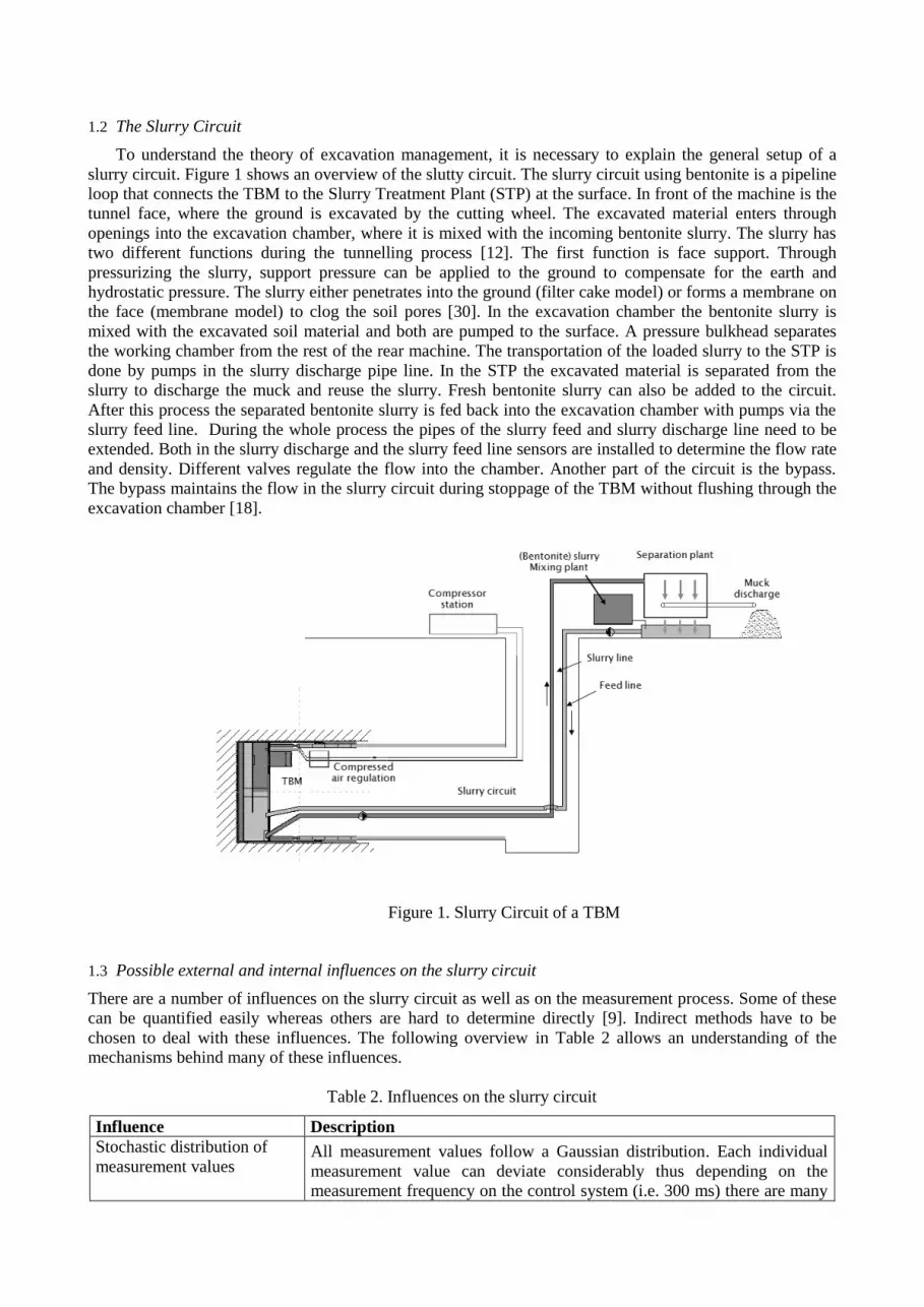
1.2 The Slurry Circuit

To understand the theory of excavation management, it is necessary to explain the general setup of a

slurry circuit. Figure 1 shows an overview of the slutty circuit. The slurry circuit using bentonite is a pipeline

loop that connects the TBM to the Slurry Treatment Plant (STP) at the surface. In front of the machine is the

tunnel face, where the ground is excavated by the cutting wheel. The excavated material enters through

openings into the excavation chamber, where it is mixed with the incoming bentonite slurry. The slurry has

two different functions during the tunnelling process [12]. The first function is face support. Through

pressurizing the slurry, support pressure can be applied to the ground to compensate for the earth and

hydrostatic pressure. The slurry either penetrates into the ground (filter cake model) or forms a membrane on

the face (membrane model) to clog the soil pores [30]. In the excavation chamber the bentonite slurry is

mixed with the excavated soil material and both are pumped to the surface. A pressure bulkhead separates

the working chamber from the rest of the rear machine. The transportation of the loaded slurry to the STP is

done by pumps in the slurry discharge pipe line. In the STP the excavated material is separated from the

slurry to discharge the muck and reuse the slurry. Fresh bentonite slurry can also be added to the circuit.

After this process the separated bentonite slurry is fed back into the excavation chamber with pumps via the

slurry feed line. During the whole process the pipes of the slurry feed and slurry discharge line need to be

extended. Both in the slurry discharge and the slurry feed line sensors are installed to determine the flow rate

and density. Different valves regulate the flow into the chamber. Another part of the circuit is the bypass.

The bypass maintains the flow in the slurry circuit during stoppage of the TBM without flushing through the

excavation chamber [18].

Figure 1. Slurry Circuit of a TBM

1.3 Possible external and internal influences on the slurry circuit

There are a number of influences on the slurry circuit as well as on the measurement process. Some of these

can be quantified easily whereas others are hard to determine directly [9]. Indirect methods have to be

chosen to deal with these influences. The following overview in Table 2 allows an understanding of the

mechanisms behind many of these influences.

Table 2. Influences on the slurry circuit

Influence Description

Stochastic distribution of

measurement values

All measurement values follow a Gaussian distribution. Each individual

measurement value can deviate considerably thus depending on the

measurement frequency on the control system (i.e. 300 ms) there are many

values available. The high number of individual measurements neutralises

the effect of the stochastic deviations.

Miscalibration All sensors must be calibrated. The calibration status will change over time

due to the physical influences on the sensor. Therefore every sensor must

be recalibrated regularly by software or hardware means to reflect these

changes. Miscalibration is one of the largest contributors to measurement

inaccuracy and can only be dealt with by careful operation and calibration

by the site personnel.

Sealing Water Sealing water is added to the seals of all pumps and valves. It partly enters

the bentonite flow and partly leaks outward. As the ratios are depending on

a multitude of changing influences, its amount is impossible to estimate

deterministically. Its influence can only be indirectly excluded from the

measurement.

Time Influence As the measurement error of density meters depends on the particle size

distribution when assembled horizontally, these are normally installed

vertically in the shaft. This leads to a time delay in density measurement

compared to flow. This time influence is visible in the mass, dry mass and

the dry volume measurement but not in the volume measurement. So the

volume measurement will still react immediately when flow sensors are

assembled in the shaft as fluids are incompressible.

Leakages Usually there are little visible leakages, but as ball valves experience

strong wear throughout projects, they develop internal leakages.

Depending on the calibration methods used to check the measurement

system, this must be considered when calibrating the sensors.

Interventions During interventions the excavation and working chamber are usually

emptied or the bentonite level is lowered. This causes the excavated

amounts for the rings during and after intervention to deviate from the

normal values.

Pipe extension During pipe extension, parts of the volume stored in the pipe are lost and

there can be an influence on the measurement.

Face Flows The ground and therefore the tunnel face are permeable and often saturated

with water. As a result there can be bentonite flows from the chamber into

the ground or groundwater inflow into the chamber. Depending on geology

and machine operation, this can be normal to a small degree if support

pressure is applied correctly. However these flows should not be allowed

to be large in order to avoid any major influence.

2. DEFINITIONS

The parameters and expressions describing excavation management vary between different countries and

different publications. This causes a lot of misunderstanding when technical information is communicated

between different parties in the industry. This Section introduces the input and output parameters for

excavation management and provides a precise foundation for further work by setting out exact

mathematical definitions for all relevant parameters. Where possible the definitions follow the Geotechnical

Engineering Handbook [28] as well as the typical industry standards.

2.1 General Definitions

The following definitions apply to the operational and geotechnical parameters which are relevant for the

excavation management system:

Solids Density is the average density of the solid materials in the ground. This refers to the solid particles

only and does not take into account the packing density or any fluids or gasses in the voids between the

particles. Therefore it depends solely on the mineral composition of the solids. Table 3 gives an overview for

a number of common minerals. The solids density is different from the dry density and a common mistake in

practice of mixing these two should be avoided.

𝑆𝑜𝑙𝑖𝑑𝑠 𝐷𝑒𝑛𝑠𝑖𝑡𝑦 = 𝜌𝑠𝑜𝑙𝑖𝑑𝑠 [𝑡𝑚3⁄ ]

Water Content is the percentage (by volume) of water in the ground. The water fills the voids between solid

(soil) particles or rock formations. The water content is defined as the ratio of volume of water to the volume

of solids. In fully saturated soil below the groundwater table, the water content is equal to the volume of

voids between the particles [7]. The difficulty in measuring the actual water content of the soil lies in

measuring it without changing its value by the disturbance created by the measurement process.

𝑊𝑎𝑡𝑒𝑟 𝐶𝑜𝑛𝑡𝑒𝑛𝑡 = 𝑛𝑤 [%]

𝑛𝑤 = 𝑉𝑤𝑎𝑡𝑒𝑟 𝑉𝑠𝑜𝑙𝑖𝑑𝑠⁄ (Eq. 1)

In Situ Density is the average density of the ground in its undisturbed state before excavation or other

interference. As there are voids between particles and rock formations which are filled with water, the actual

in situ density is always lower than the solids density or the dry density defined below. In fully saturated

soils, all voids are completely filled with water. Therefore the in situ density can be defined as the follows:

𝐼𝑛 𝑆𝑖𝑡𝑢 𝐷𝑒𝑛𝑠𝑖𝑡𝑦 = 𝜌𝑖𝑛 𝑠𝑖𝑡𝑢 [𝑡𝑚3⁄ ]

𝜌𝑖𝑛 𝑠𝑖𝑡𝑢 = 𝜌𝑠𝑜𝑙𝑖𝑑𝑠 × (1 − 𝑛𝑤) + 𝑛𝑤 (Eq. 2)

Dry Density is the bulk density of the solid material without any water filling the voids. It depends on the

solids density and the compaction of the material. ASTM D4254 [1] defines it as the ratio of dry solid mass

per bulk volume. A density index developed by Terzhagi [28] can be used to define the relative compaction

level between maximum and minimum packing density. It should be remembered that the dry density is less

than and not equal to the solids density.

𝐷𝑟𝑦 𝐷𝑒𝑛𝑠𝑖𝑡𝑦 = 𝜌𝑑𝑟𝑦 [𝑡𝑚3⁄ ]

𝜌𝑑𝑟𝑦 = 𝑚𝑑𝑟𝑦 𝑉𝑏𝑢𝑙𝑘⁄ (Eq. 3)

Bentonite Powder Density is the solids density of the bentonite powder which depends only on its mineral

composition. This density is very similar to the particle density of the soil and many dry mass calculation

formulae are simplified in such a way that it is assumed as the same as the solids density of the ground.

𝐵𝑒𝑛𝑡𝑜𝑛𝑖𝑡𝑒 𝑃𝑜𝑤𝑑𝑒𝑟 𝐷𝑒𝑛𝑠𝑖𝑡𝑦 = 𝜌𝑏𝑒𝑛𝑡𝑜𝑛𝑖𝑡𝑒 [𝑡𝑚3⁄ ]

Feed Slurry Density is the density of the bentonite suspension in the slurry feed line. Its value depends on

the type and quality of freshly mixed bentonite suspension as well as on the fines content from excavated

muck which is accumulating in the slurry until removed in the separation plant.

𝐹𝑒𝑒𝑑 𝑆𝑙𝑢𝑟𝑟𝑦 𝐷𝑒𝑛𝑠𝑖𝑡𝑦 = 𝜌𝑓𝑒𝑒𝑑 [𝑡𝑚3⁄ ]

Discharge Slurry Density is the density of the bentonite suspension in the discharge line. The density is a

resultant of mixing muck into the bentonite suspension in the excavation chamber. Sometimes it is referred

to as discharge density.

𝐷𝑖𝑠𝑐ℎ𝑎𝑟𝑔𝑒 𝑆𝑙𝑢𝑟𝑟𝑦 𝐷𝑒𝑛𝑠𝑖𝑡𝑦 = 𝜌𝑑𝑖𝑠𝑐ℎ𝑎𝑟𝑔𝑒 [𝑡𝑚3⁄ ]

Feed Slurry Flow is the flow rate in the slurry feed line. As fluids are incompressible it is always constant at

every point in the slurry circuit.

𝐹𝑒𝑒𝑑 𝐹𝑙𝑜𝑤 = �̇�𝑓𝑒𝑒𝑑 [𝑚3

ℎ⁄ ]

Discharge Slurry Flow is the flow rate in the discharge line. It is usually higher than the slurry feed flow as

there is sealing water and muck mixed into the discharge flow. As for the slurry feed flow rate, the discharge

flow is constant throughout the whole circuit as fluids are incompressible [13].

𝐷𝑖𝑠𝑐ℎ𝑎𝑟𝑔𝑒 𝐹𝑙𝑜𝑤 = �̇�𝑑𝑖𝑠𝑐ℎ𝑎𝑟𝑔𝑒 [𝑚3

ℎ⁄ ]

Chamber Volume is the volume of material in the excavation chamber of the TBM. This is usually constant

for TBMs with a single chamber while in TBMs with a double chamber and air bubble the volume of muck

stored can vary as the face support pressure is regulated to maintain a constant pressure while the filling level

can change. The fluctuation over time should be considered in an excavation management system by

measuring the level in the second chamber. This change is then calculated over time and included in the

excavation management system [10].

𝐶ℎ𝑎𝑚𝑏𝑒𝑟 𝑉𝑜𝑙𝑢𝑚𝑒 𝐶ℎ𝑎𝑛𝑔𝑒 =△ 𝑉𝑐ℎ𝑎𝑚𝑏𝑒𝑟 [𝑚³]

2.2 Target Value Definitions

The definitions outline the various target parameters which are used in excavation management systems. One

aspect which should be considered regardless of the actual parameters used is their dependency on the

geological situation. Nakano et al. explain how the different weathering grades of granite along the tunnel

alignment influence the target solids volume [20]. The dry solid volume of moderately weathered granite

(GIII) could be for example twice as that of residual soil (GVI). Referring to this, the interpretation of a

higher excavated dry solids volume in comparison to the target volume can be different. It can occur either

because of over-excavation or through rapid change in the ground conditions [26].

Figure 2. Target Dry Solids volume depending on ground conditions [20]

Theoretical Dry Mass is the theoretical in situ mass of excavated solids. This value can potentially form the

reference value of an excavation management system. The practical difficulty in obtaining the value lies in

the challenge of measuring the bulk density and water content reliably. As this depends on the weathering

grade as well as the size, orientation and distribution of rock joints or other features of the ground, it can

change rapidly from ring to ring. Also by attempting an in situ measurement, one might change the packing

density and therefore the water content [7], [8]. The theoretical dry mass plays an important role in practical

application as it is possible to measure it in the slurry circuit as well as to some extent on belt scales. Thereby

it allows independent double measurement of the same parameter.

𝑇ℎ𝑒𝑜𝑟𝑒𝑡𝑖𝑐𝑎𝑙 𝐷𝑟𝑦 𝑀𝑎𝑠𝑠 = 𝑚𝑑𝑟𝑦,𝑡ℎ𝑒𝑜𝑟 [𝑡]

𝑚𝑑𝑟𝑦,𝑡ℎ𝑒𝑜𝑟 = 𝐴𝑓𝑎𝑐𝑒 ×△ 𝑙𝑎𝑑𝑣𝑎𝑛𝑐𝑒 × (1 − 𝑛𝑤) × 𝜌𝑠𝑜𝑙𝑖𝑑𝑠 (Eq. 4)

Theoretical Solids Volume is the volume of excavated solids. This value does not consider the packing

density of the soil or rock particles and does not change with varying compaction level. In fully saturated

soil, the theoretical solids volume for one ring can be determined by deducting the water content from the

total volume [28]. The practical determination of solids volume cannot be done easily. It can only be

measured by using fluids and their displacement which is an indirect measurement method that cannot be

performed for large volumes on site. Nonetheless dry solids volume can be an important measure as a

reference value in an excavation management system as it can be estimated based on water (moisture)

content normally defined in the geotechnical baseline report.

𝑇ℎ𝑒𝑜𝑟𝑒𝑡𝑖𝑐𝑎𝑙 𝑆𝑜𝑙𝑖𝑑𝑠 𝑉𝑜𝑙𝑢𝑚𝑒 = 𝑉𝑠𝑜𝑙𝑖𝑑𝑠,𝑡ℎ𝑒𝑜𝑟 [𝑚³]

𝑉𝑠𝑜𝑙𝑖𝑑𝑠,𝑡ℎ𝑒𝑜𝑟 = 𝐴𝑓𝑎𝑐𝑒 ×△ 𝑙𝑎𝑑𝑣𝑎𝑛𝑐𝑒 × (1 − 𝑛𝑤) (Eq. 5)

Theoretical Dry Volume is the bulk volume of the dry material. It depends mainly on the relative

packing density of the material and changes easily when the ground is disturbed by any interaction or

external influences. Therefore it is hard to define in general but can only be defined for a certain state the

material is in with the current porosity “n”. When using it as a reference for an excavation management

system which is done regularly, this difficulty must be considered. Also any comparison to the material in

the muck pit is incorrect as the porosity (in the muck pit) differs totally from that in the ground.

Nonetheless dry volume plays an important role as a possible reference value for excavation management

systems.

𝑇ℎ𝑒𝑜𝑟𝑒𝑡𝑖𝑐𝑎𝑙 𝐷𝑟𝑦 𝑉𝑜𝑙𝑢𝑚𝑒 = 𝑉𝑑𝑟𝑦,𝑡ℎ𝑒𝑜𝑟 [𝑚³]

𝑉𝑑𝑟𝑦,𝑡ℎ𝑒𝑜𝑟 = 𝑉𝑠𝑜𝑙𝑖𝑑𝑠 × (1 − 𝑛) (Eq. 6)

Theoretical Volume is the volume theoretically excavated from the ground. This volume contains all solids

and water. It depends on the mechanism of slurry penetration into the ground and the formation of filter cake

as shown in Figure 3. This mechanism defines, how much ground water is displaced by the slurry or how

much is entering the chamber and is discharged with the solids [25]. Following formula assumes that all

water present at the tunnel face will be excavated. The real value lies between this theoretical volume and the

theoretical solids volume. It can vary during excavation according to ground properties. Therefore a range of

results should be seen as correct instead of just one number.

𝑇ℎ𝑒𝑜𝑟𝑒𝑡𝑖𝑐𝑎𝑙 𝑉𝑜𝑙𝑢𝑚𝑒 = 𝑉𝑡ℎ𝑒𝑜𝑟 [𝑚³]

𝑉𝑡ℎ𝑒𝑜𝑟 = 𝐴𝑓𝑎𝑐𝑒 ×△ 𝑙𝑎𝑑𝑣𝑎𝑛𝑐𝑒 (Eq. 7)

Figure 3. Mechanisms of tunnel face support and excavation [30]

Theoretical Mass is the mass of excavated materials. This value contains all solids and water which are

excavated. Similar to the theoretical volume, there is a certain range which is to be expected depending on

the mechanisms of face support. The following formula poses a theoretical value which can decrease when

considering bentonite losses into the soil or increase if excess ground water is discharged.

𝑇ℎ𝑒𝑜𝑟𝑒𝑡𝑖𝑐𝑎𝑙 𝑀𝑎𝑠𝑠 = 𝑚𝑡ℎ𝑒𝑜𝑟 [𝑡]

𝑚𝑡ℎ𝑒𝑜𝑟 = 𝐴𝑓𝑎𝑐𝑒 ×△ 𝑙𝑎𝑑𝑣𝑎𝑛𝑐𝑒 × 𝜌𝑖𝑛 𝑠𝑖𝑡𝑢 (Eq. 8)

3. EXCAVATION MANAGEMENT FORMULAE

At present the industry uses a number of different formulae to calculate the results presented by excavation

management systems. The formulae are used for calculating different types of final results such as those

mentioned in Section 2 and utilize different input parameters which have to be keyed in by the user. This

Section introduces common approaches adopted at present by different suppliers and contractors and

explains these in more detail.

3.1 Calculation of Excavated Volume

The excavated volume can be calculated by integrating the difference between feed and discharge flow rate

over time as well as adding the changes if any in chamber volume. The input values for excavated volume

calculation come from the flow meters as well as from the chamber level sensor in those TBMs with a

second chamber. In case of single chamber TBMs, the calculation relies only on feed and discharge flow

meter readings. As the flow volume measurement is very sensitive, there are many factors which can affect

the calculation results but which cannot be automatically included into the calculation algorithm as these

cannot be measured directly. Such factors are: a) the pipe extension, b) chamber interventions, c)

measurement inaccuracies of the flow meters due to frequent starting and stopping of the slurry circuit, d)

sealing water, or e) flows at the cutterhead through the face. Furthermore the volume balance is very

sensitive to sensor miscalibration. Therefore a purely volume based system is very challenging to calibrate

and manage excavation reliably.

𝑉𝑒𝑥𝑐𝑎𝑣𝑎𝑡𝑒𝑑 = ∫ [(�̇�𝑑𝑖𝑠𝑐ℎ𝑎𝑟𝑔𝑒 − �̇�𝑓𝑒𝑒𝑑)]𝐴𝑑𝑣𝑎𝑛𝑐𝑒 𝐸𝑛𝑑

𝐴𝑑𝑣𝑎𝑛𝑐𝑒 𝑆𝑡𝑎𝑟𝑡𝛿𝑡 +△ 𝑉𝑐ℎ𝑎𝑚𝑏𝑒𝑟 (Eq. 9)

3.2 Calculation of Deviation Flow Volume

Deviation Flow Volume is the cumulative volume calculated from the Deviation Flow Rate. The Deviation

Flow Rate is the discrepancy between slurry feed flow and the amount of slurry discharge flow and

theoretical excavation flow and is defined in the following formula. It utilizes the excavation face area (Aface)

and jack speed of the machine (s). Over-excavation or a high water inflow into the chamber can be seen in a

positive Deviation Flow Volume. Negative Deviation Flow Volume can be caused by a slurry loss into the

ground. The deviation flow is therefore a parameter which is directly related to the excavated volume and

the objective is to keep it at zero or slightly below zero. It is used as an indicator showing the trend of

volume during excavation [29].

△ 𝑄 = 𝑄𝑑𝑖𝑠𝑐ℎ𝑎𝑟𝑔𝑒 − (𝑄𝐹𝑒𝑒𝑑 + 𝐴𝑓𝑎𝑐𝑒 × 𝑠) (Eq. 10)

3.3 Calculation of Excavated Mass

The excavated mass can be calculated by integrating the difference of feed and discharge mass flows [32].

Additionally the change in stored mass in the working chamber must be considered if the TBM is equipped

with an air bubble chamber. The density in the chamber equals the density in the discharge line which allows

calculating the stored mass from the level reading. The mass flow can be measured by multiplying flow

volume and density meter readings of each line. All measurement errors and influences on the volume flow

measurement also affect the mass measurement. Therefore a mass based measurement system is very

challenging to calibrate precisely as well.

𝑚𝑒𝑥𝑐𝑎𝑣𝑎𝑡𝑒𝑑 = ∫ [(�̇�𝑑𝑖𝑠𝑐ℎ𝑎𝑟𝑔𝑒 × 𝜌𝑑𝑖𝑠𝑐ℎ𝑎𝑟𝑔𝑒 − �̇�𝑓𝑒𝑒𝑑 × 𝜌𝑓𝑒𝑒𝑑)]𝐴𝑑𝑣𝑎𝑛𝑐𝑒 𝐸𝑛𝑑

𝐴𝑑𝑣𝑎𝑛𝑐𝑒 𝑆𝑡𝑎𝑟𝑡𝛿𝑡 +△ 𝑉𝑐ℎ𝑎𝑚𝑏𝑒𝑟 × 𝜌𝑑𝑖𝑠𝑐ℎ𝑎𝑟𝑔𝑒 (Eq. 11)

3.4 Excavated Dry Mass

As many of the measurement errors in excavation management systems originate in the volume flow

measurement which is influenced by many events on the machine, calculating the dry mass eliminates most

of these influences from the calculation results. Therefore dry mass and dry volume based excavation

management systems offer the advantage of being less unstable and easier to calibrate. Their downside is that

they do not indicate the influence of groundwater clearly. Generally for a given amount of material, the dry

mass can be calculated when the individual densities of solids and water as well as the total density of the

mixture is known. Practically the excavated dry mass can be calculated from the density and flow readings of

both lines, given the individual densities of the rock or soil particles are known [35]. Figure 4 and following

formula illustrate the principle of this approach:

𝑚𝑑𝑟𝑦 = 𝑉𝑡𝑜𝑡𝑎𝑙 ∗𝜌𝑡𝑜𝑡𝑎𝑙−𝜌𝑤𝑎𝑡𝑒𝑟

𝜌𝑠𝑜𝑙𝑖𝑑−𝜌𝑤𝑎𝑡𝑒𝑟∗ 𝜌𝑠𝑜𝑙𝑖𝑑𝑠 (Eq. 12)

Figure 4. Dry mass in relation to total mass and volume [3]

This formula is applied to the feed and the discharge material and the result will be the excavated dry mass.

As there are various forms of development by different contractors and different TBM suppliers for

excavation management system, there are a number of different formulae which are used throughout the

industry. They differ mainly in the type of simplifications which are adopted. Also some use different input

values depending on the preference of the TBM supplier or operator. The simplifications are necessary to not

overcomplicate the measurement process and allow smooth operation on site. The following Section presents

a number of different approaches in the calculation of the amount of dry solids material excavated.

a) Calculation based on Particle and Bentonite Density: In order to calculate the excavated dry mass, the inflow and outflow of solids can be calculated and

once the inflow is subtracted from the outflow, the excavated dry material remains [23] [30].

The feed dry mass can be calculated as:

𝑚𝑓𝑒𝑒𝑑,𝑑𝑟𝑦 = �̇�𝑓𝑒𝑒𝑑 ×𝜌𝑓𝑒𝑒𝑑−𝜌𝑤𝑎𝑡𝑒𝑟

𝜌𝑏𝑒𝑛𝑡𝑜𝑛𝑖𝑡𝑒−𝜌𝑤𝑎𝑡𝑒𝑟× 𝜌𝑏𝑒𝑛𝑡𝑜𝑛𝑖𝑡𝑒 (Eq. 13)

The discharge dry mass flow can be calculated as:

𝑚𝑑𝑖𝑠𝑐ℎ𝑎𝑟𝑔𝑒,𝑑𝑟𝑦 = �̇�𝑑𝑖𝑠𝑐ℎ𝑎𝑟𝑔𝑒 ×𝜌𝑑𝑖𝑠𝑐ℎ𝑎𝑟𝑔𝑒−𝜌𝑤𝑎𝑡𝑒𝑟

𝜌𝑠𝑜𝑙𝑖𝑑𝑠−𝜌𝑤𝑎𝑡𝑒𝑟× 𝜌𝑠𝑜𝑙𝑖𝑑𝑠 (Eq. 14)

The resulting excavated dry mass for one ring can therefore be determined by considering the change

during a given time period “t” :

𝑚𝑑𝑟𝑦 = ∫ (�̇�𝑑𝑖𝑠𝑐ℎ𝑎𝑟𝑔𝑒 ×𝜌𝑑𝑖𝑠𝑐ℎ𝑎𝑟𝑔𝑒 − 𝜌𝑤𝑎𝑡𝑒𝑟

𝜌𝑠𝑜𝑙𝑖𝑑𝑠 − 𝜌𝑤𝑎𝑡𝑒𝑟

× 𝜌𝑠𝑜𝑙𝑖𝑑𝑠 − �̇�𝑓𝑒𝑒𝑑 ×𝜌𝑓𝑒𝑒𝑑 − 𝜌𝑤𝑎𝑡𝑒𝑟

𝜌𝑏𝑒𝑛𝑡𝑜𝑛𝑖𝑡𝑒 − 𝜌𝑤𝑎𝑡𝑒𝑟

× 𝜌𝑏𝑒𝑛𝑡𝑜𝑛𝑖𝑡𝑒) 𝛿𝑡

𝑅𝑖𝑛𝑔 𝑒𝑛𝑑

𝑅𝑖𝑛𝑔 𝑠𝑡𝑎𝑟𝑡

+ △ 𝑉𝑐ℎ𝑎𝑚𝑏𝑒𝑟 × 𝜌𝑑𝑖𝑠𝑐ℎ𝑎𝑟𝑔𝑒 (Eq. 15)

This approach requires knowledge of the ground particle density which can be determined precisely as

well as of the bentonite powder density. Both need to be keyed in by the operator or must be

hardcoded in the software system. The last expression which includes the effect of changing chamber

levels into the formula can only be approximated as the actual chamber density is not homogenous.

Therefore this section represents a mass instead of a dry mass which allows the closest possible

approximation.

This formula is the theoretically correct method of calculating the excavated dry mass. It can be

simplified as shown in sub-section b) below.

b) Calculation based on generalized solids density and fixed water density:

𝑚𝑑𝑟𝑦 = ∫ (�̇�𝑑𝑖𝑠𝑐ℎ𝑎𝑟𝑔𝑒 × (𝜌𝑑𝑖𝑠𝑐ℎ𝑎𝑟𝑔𝑒 − 1) − �̇�𝑓𝑒𝑒𝑑 × (𝜌𝑓𝑒𝑒𝑑 − 1)

𝜌𝑝𝑎𝑟𝑡𝑖𝑐𝑙𝑒 − 1× 𝜌𝑝𝑎𝑟𝑡𝑖𝑐𝑙𝑒) 𝛿𝑡




This formula is a simplification of a) that does not take into account the possible density differences

between bentonite and ground particles. As this difference is usually very small, the ensuing error is

considered to be very small compared to possible other sources of errors. Table 3 gives an overview of

different minerals densities. This formula allows a useful simplification in the operation of an

excavation management system, as keying in bentonite density can be omitted and assumed equal to

ground particle density. Also fixing water density at 1 t/m³ is a reasonable simplification that makes

sense and simplifies the operation. This formula is also used in the paper from Yamazaki et al [34] in

1984.

Table 3. Solids densities of several minerals in g/cm³ [22]

Gypsum 2,32 Montmorillonite 2,75-2,78

Feldspar 2,55 Mica 2,80-2,90

Kaolinite 2,64 Dolomite 2,85-2,95

Quartz 2,65 Biotite 2,80-3,20

Na-feldspar 2,62-2,76 Amphibole 3,10-3,40

Calcite 2,72 Barite 4,48

Illite 2,60-2,86 Magnetite 5,17

c) Calculation based on In Situ Density

𝑚𝑑𝑟𝑦 = ∫ (𝜌𝑑𝑖𝑠𝑐ℎ𝑎𝑟𝑔𝑒 × �̇�𝑑𝑖𝑠𝑐ℎ𝑎𝑟𝑔𝑒 − 𝜌𝑓𝑒𝑒𝑑 × �̇�𝑓𝑒𝑒𝑑

𝜌𝑖𝑛 𝑠𝑖𝑡𝑢 − 𝜌𝑓𝑒𝑒𝑑

) 𝛿𝑡 △ 𝑉𝑐ℎ𝑎𝑚𝑏𝑒𝑟 × 𝜌𝑑𝑖𝑠𝑐ℎ𝑎𝑟𝑔𝑒 (Eq. 17)



This formula allows calculation based on in situ density. This means that the solids density and

bentonite density need not be known but only the in situ density of the ground. This allows an easier

comparison with the theoretically excavated dry mass as a target. This value is also calculated based

on the same in situ density. Therefore there is no need for different input parameters for target and

measurement such as separate particle density and ground water content. This formula is a typical

example of an approximation which is not scientifically correct but used on site for several projects in

the US. The theoretical incorrectness becomes obvious when calculating the units in the formula which

are incorrect.

d) Mixed Calculation Based on Particle and In Situ Density

𝑚𝑑𝑟𝑦 = ∫ (�̇�𝑑𝑖𝑠𝑐ℎ𝑎𝑟𝑔𝑒 × (𝜌𝑑𝑖𝑠𝑐ℎ𝑎𝑟𝑔𝑒 − 1) − �̇�𝑓𝑒𝑒𝑑 × (𝜌𝑓𝑒𝑒𝑑 − 1)

(𝜌𝑖𝑛 𝑠𝑖𝑡𝑢 − 𝜌𝑓𝑒𝑒𝑑)) 𝛿𝑡 ×

𝜌𝑠𝑜𝑙𝑖𝑑𝑠

(𝜌𝑠𝑜𝑙𝑖𝑑𝑠 − 1)




The given formula is another calculation based on in situ density. It is an extension of the formula

mentioned in c). Different to the previous formula the density of water, again simplified to 1 t/m3, is

included. The Formula also assumes knowledge of the particle density. Similar to the formula

mentioned in c), this formula is not scientifically correct but an approximation which has been used in

a number of projects. As with the formula shown in c) the units in this formula are incorrect.

e) Calculation of Solids Material Volume

𝑉𝑠𝑜𝑙𝑖𝑑𝑠 = ∫ (�̇�𝑠𝑙𝑢𝑟𝑟𝑦 ×𝜌𝑑𝑖𝑠𝑐ℎ𝑎𝑟𝑔𝑒 − 1

𝜌𝑠𝑜𝑙𝑖𝑑𝑠 − 1− �̇�𝑓𝑒𝑒𝑑 ×

𝜌𝑓𝑒𝑒𝑑 − 1

𝜌𝑠𝑜𝑙𝑖𝑑𝑠 − 1) 𝛿𝑡 △ 𝑉𝑐ℎ𝑎𝑚𝑏𝑒𝑟 ×

𝜌𝑑𝑖𝑠𝑐ℎ𝑎𝑟𝑔𝑒

𝜌𝑠𝑜𝑙𝑖𝑑𝑠

(Eq. 19)



This formula is applied for calculating the Solids Material Volume [21]. The last sequence includes the

addition of the volume of the chamber level change. It is essentially based on dry mass calculation

methods but is shortened by deleting the density multipliers from the calculation. This allows

calculating only the solids volume. The actual dry volume cannot be measured as the packing density

of the particles changes constantly while handling. The upper and lower boundaries are shown in

Figure 5. In the published literature and practice it can often be found that the solids material volume is

called dry material volume. This ambiguity is theoretically incorrect but seldom discussed in practice

as its influence is marginal compared to many other effects.

Figure 5. Loosest (a) and densest (b) packing of spheres [28]

4. MEASUREMENT HARDWARE

The measurement of the excavated quantity of material takes place directly in the slurry circuit and TBM

working chamber. A number of sensors to measure flow rate, density and level are arranged in such a way

that they can measure the flow volume and density in the system for the determination of the excavated

quantity of material.

4.1 Flow Meters

The tunneling industry is generally using electromagnetic flow meters at present. Their accuracy typically

depends on the uniformity of flow, the even distribution of solids and the flow speed in the pipe as well as

the behavior of the solids [27]. Typically in TBMs the magnetic flow meters are operated at the lower end of

their permissible flow speed range. Below a certain flow speed, the stochastic measurement errors increase.

This effect starts usually below around 2 m/sec [13] as can be seen in Figure 6. Nonetheless this error does

not affect the practical measurement dramatically, as the large number of individual readings and the

stochastic nature of the error leads to a strong equalization effect. The sensors in feed line and discharge line

must be calibrated relative to each other. In case they have an offset between their calibrations, this will

directly affect any measurement significantly [36]. Therefore it is necessary to spend considerable effort on

the relative calibration of the flow meters [24]. This can only be done when the machine is driven in bypass

mode regularly.

Figure 6. Stochastic measurement deviation and flow meter principle

4.2 Density Sensors

The density meters installed in slurry shields are usually based on the gamma ray transmission method. On

one side of the pipe there is a gamma ray source and a scintillation counter on the other side. The radiation

through the pipe is weakened by matter. The denser the matter is, the less will be measured on the other side.

An accurate measurement strongly depends on the uniformity of solids distribution inside the pipe. Therefore

sensor suppliers recommend installation of the density meter in a vertical section of pipe [11] [3]. Figure 7

shows a density meter and its components. When looking at the gamma ray passing through the pipe, it

becomes obvious that the measurement can only be accurate when the solids are evenly distributed radially

[31]. This is the usual case in vertical sections of pipe. Horizontal measurement may be feasible in cases

where the particle size distribution does not change within a project which is hardly the case. The location of

the density meter is critical to the accuracy of the readings. Experiments suggest that a minimum of 10

diameters length of straight vertical pipe before and 3 diameters after the density meter is necessary to

achieve a precise measurement [31]. Furthermore, to maintain the accuracy of measurement the meter needs

to be calibrated regularly [15] by operating the TBM in bypass mode for sufficiently long period.

Figure 7. Density meter components [3] and transmission through pipe

4.3 Level Sensors

In TBMs which utilize an air bubble chamber for pressure control, the slurry level of working chamber must

be measured and included in the calculation of the excavation management system. The sensor type normally

used is a rope sensor which is sensitive to mechanical disruption and damage [14]. Therefore the

functionality and correctness of the rope sensor readings must be checked regularly.

5. SIMULATION OF EXCAVATED MATERIAL CALCULATION

In order to test and visualize different calculation approaches described in Section 3 and analyze how these

respond to certain conditions and events an Excel based simulation framework has been developed. This

allows the definition of various input scenarios and determine the consequences for the slurry circuit and its

operating parameters.

The measurements and readings from the sensors are used as input data. The different calculation algorithms

are then implemented in the simulation to produce different output corresponding to the calculation methods.

Then the output of the different algorithm results are plotted and compared to target curves.

5.1 The Simulation Framework

This Section describes the Excel simulation tool which is based on a linear model that can accommodate

different scenarios during the tunneling process. The tool includes two implementation sheets and one for

visualization of the results. The first one is a table with fixed constants, the second is a calculation sheet with

the output data and the third one includes graphs showing the results of the calculations. The input sheet

contains all user defined input data which are used for the calculation. This includes soil property, tunnel

geometry, slurry circuit data and sensor properties. The calculation sheet defines the different scenarios

mathematically. The scenarios are specific events at the tunnel face, in the excavation chamber and in the

slurry circuit. Figure 8 shows a screenshot of the simulation framework. With the help of the formulae

explained in Section 3, the results in terms of volume, mass, dry mass and dry volume for each scenario are

shown. The comparison of the results obtained from each formula can be done for different scenarios to see

how different formulae perform during these scenarios. The main parameters input are as follows:

Rock Density

Water Content

Bentonite Powder Density

Tunnel Diameter

Ring Length

Solids and Water Inflow Rates

Sensor Calibration

Advance speed

Sensor Accuracy

Flow Rates

Chamber Level

Theoretical Target Parameters

Figure 8. The simulation calculation sheet with input (left) and output (right)

5.2 Simulation Scenarios

The different ways of monitoring a slurry circuit offers both advantages and disadvantages. Depending on

the type of calculation, some events might even go unnoticed [16]. Therefore a thorough check is necessary.

Stochastic methods can support this [33]. Following scenarios shown in Table 4 are checked separately and

the results are compared against target values for accuracy.

Table 4. Definition of simulated scenarios

Standard Ring Excavation

Simulation of a standard ring excavation without any extraordinary

event. The ground properties are fixed at GVI parameters and there is

no over or under-excavation. This introductory comparison shows the

different behaviours of each calculation approach.

Varying Geology

Simulation of two rings with different geological conditions. First full

face rock GIII, second soil GVI. No over- or under-excavation

occurring. This test shows how different formulae compare in

varying geology.

Sudden Face Collapse

Sudden inflow of solids which displace bentonite. The displaced

bentonite fills the cavity left by the collapsed material. Thus no

significant volume increase occurs in the chamber.

Over-excavation / Sudden

Water Inflow

Simulation of continuous over-excavation in soil and simulation of

encountering water bearing joints in a GIII rock formation. No

additional solids enter the chamber but extra water flows in while

mining past the rock fissure.

Flow Meter Miscalibration



no over or under-excavation. The influence of flow sensor

miscalibration is shown by manipulating the readings.

Density Meter Miscalibration



no over or under-excavation. The influence of density sensor

miscalibration is shown by manipulating the readings.

Incorrect Particle Density



no over or under-excavation. The influence of an incorrect particle

density setting used for the dry mass calculation is shown.

In the simulation tool one theoretical ring is created on which the effects of different scenarios are applied

and the results with different formulae are demonstrated. The example ring in this Excel tool is built during a

total cycle time of 2 h. The advance time amounts to 1.5 h, including 5 min bypass mode at the end. The next

30 min is the standstill during ring building, which also ends with 5 min bypass mode before the next ring.

During the TBM advance a constant mining rate is considered. The different scenarios which are compared

are staged in typical geological conditions in Singapore. Data from Circle Line project [26], [20] has been

used to simulate GIII and GVI Bukit Timah Granite. Water and solid content of the ground material are

based on the data presented in Figure 2. All calculations assume an average particle density of the soil and

rock minerals of:

𝜌𝑠𝑜𝑙𝑖𝑑𝑠 = 2.65 [𝑡𝑚3⁄ ]

The sensors are put in individually in the simulation so miscalibration can be addressed and visualized in the

result graphs. Furthermore the parameters which have to be input by the users of excavation management

systems can be adjusted in the simulation so that possibly wrong values can be simulated and the

consequences can be studied.

6. RESULTS

In order to compare the behavior of the different formulae, the results of different simulation conditions are

shown in a condensed form. All results are presented first and the inaccurate calculation approaches are

eliminated from further consideration. Subsequently comparisons are carried out for the scenarios described

in Section 5. Figure 9 shows the outcome from the first simulation and the general principles for comparison

of results. While a certain scenario is studied by the simulation tool, the resulting curves are plotted for all

calculation methods.

6.1 Standard ring excavation

Figure 9. The simulation results for all calculation approaches for standard ring

Figure 9 shows an overview of results for different calculation approaches and target curves. The plot on the

left side shows different dry mass and dry volume obtained from the simulation tool. The plot on the right

side shows the values from manual analysis of the ground conditions as well as excavated total mass and

total volume. With regards to the 5% maximum deviation of the results which is often stated or demanded,

the 20% spread between different dry mass calculation formulae is unacceptable. As a first consequence, the

dry mass formulae using in situ density is seen to produce results that lie too far away from the theoretical

target values and therefore should be ruled out from usage. When comparing the theoretical dry mass with

the two remaining dry mass formulae, our initial assumption that the dry mass formulae using generalized

particle density and fixed water density are fairly accurate. Their deviation from the target line is small

enough to be used practically without loss of accuracy. The solids material volume formula produces an

accurate result as well. But the solids volume of a sample of excavated material is practically difficult to

measure. It is not easy to double check the results obtained on site within the required level of accuracy.

Therefore the following steps of this study focus on the comparison of the dry mass with a generalized solids

and fixed water density to the total mass and total volume measurements.

6.2 Influence of varying geological conditions

The formulae react differently to varying ground conditions. Nakano et al. have analysed how the rock / soil

distribution in Bukit Timah Granite affects the expected dry soil volume [20]. The comparison shown in

Figure 2 is analysed using the simulation tool and the output for mass, volume and dry mass are compared.

The results of this comparison are shown in Figure 10. An interesting observation is that the total volume is

not strongly affected by the type of geology when the membrane model for face support is applied as there is

no major bentonite loss assumed. However in sand, gravel or in rock with wide joints this assumption may

not be correct as bentonite losses are likely. The mass measurement shows a higher dependency on the

geological variance. While the readings in GIII are still in a range of approximately 110 t, the readings for

GVI are strongly governed by the different densities of water and soil and therefore reduced to nearly 90 t.

This result is close to the ring volume multiplied by the in situ density.

Figure 10. Simulation results for GIII and GVI Bukit Timah Granite

The excavated dry mass readings show the clearest difference when tunnelling through varying geologies. As

the water content of GVI is high that the solids volume makes up only around 50% of the total volume, and

the dry mass drops accordingly. The measurement deviation increases as well with increasing water content.

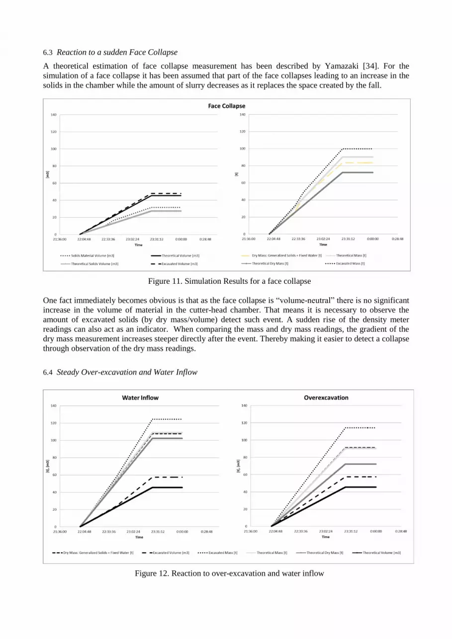
6.3 Reaction to a sudden Face Collapse

A theoretical estimation of face collapse measurement has been described by Yamazaki [34]. For the

simulation of a face collapse it has been assumed that part of the face collapses leading to an increase in the

solids in the chamber while the amount of slurry decreases as it replaces the space created by the fall.

Figure 11. Simulation Results for a face collapse

One fact immediately becomes obvious is that as the face collapse is “volume-neutral” there is no significant

increase in the volume of material in the cutter-head chamber. That means it is necessary to observe the

amount of excavated solids (by dry mass/volume) detect such event. A sudden rise of the density meter

readings can also act as an indicator. When comparing the mass and dry mass readings, the gradient of the

dry mass measurement increases steeper directly after the event. Thereby making it easier to detect a collapse

through observation of the dry mass readings.

6.4 Steady Over-excavation and Water Inflow

Figure 12. Reaction to over-excavation and water inflow

Continuous over-excavation and water inflow are two phenomena which are mainly determined by

sufficiency of the face pressure. If the face pressure is low in rock, there will be sudden water inflow in case

a water bearing fissure is encountered. This has been simulated partway during the excavation of a ring in the

graph in Figure 12, left side. The right side graph shows the curves for a steady over excavation, which

might occur in homogenous soil with insufficient face pressure.

When discussing water inflow there is an important difference between dry mass or solids volume on one

hand and mass or volume on the other hand. Due to the principle of dry mass or solids volume calculation,

additional water ingress cannot be detected. This can be seen in the left side graph in Figure 12. While the

volume and the mass graphs react immediately to the inflow, the dry mass graph does not.

As a steady over-excavation scenario means constant additional inflow of solids and water, it can be detected

by of all the different results. The magnitude of deviation depends on the water content of the ground. The

higher the water content, the clearer is the difference between dry material method and total material method.

6.5 Flow and Density Meter Miscalibration

Sensor miscalibration is a very common and frequent issue on site which is often not addressed properly.

The relationship between sensor miscalibration and the deviation of the final result is often largely

underestimated. A sensor error of a few percentages alone may in some cases lead to a final result of a ring

being far off the target values. The simulation has been used to show this influence as seen in Figure 13 for

flow meter miscalibration on the left side and for density meter miscalibration on the right side. The density

meter miscalibration has a very large influence on the final results. The flow volume has been assumed to be

5m³ above the target volume in the slurry discharge line for the left hand side graph while the density has

been assumed to be 2% too high in the slurry discharge line which corresponds to a deviation of 0.022 m³/t.

Figure 13. The influence of sensor miscalibration

The results from miscalibrated flow meters simulations demonstrate a proportional deviation of mass and

volume during excavation. The dry mass is less strongly affected by the miscalibration of the flow meter as

the percentage of solids in the slurry lines is rather small. This leads to the measurement error being kept

small which is an advantage of using dry mass or volume formulae. During bypass the values will quickly

deviate strongly if the flow meters are miscalibrated. Again this influence is reduced for the dry material

calculation.

The miscalibration of the density meter has very severe consequences. This can be seen in the right hand side

graph in Figure 13. While the slurry discharge line density meter is miscalibrated by only 2%, the apparent

increase in the excavated dry mass is almost 90% while the excavated mass is close to 50%. This underlines

the importance of the accuracy of the sensor hardware.

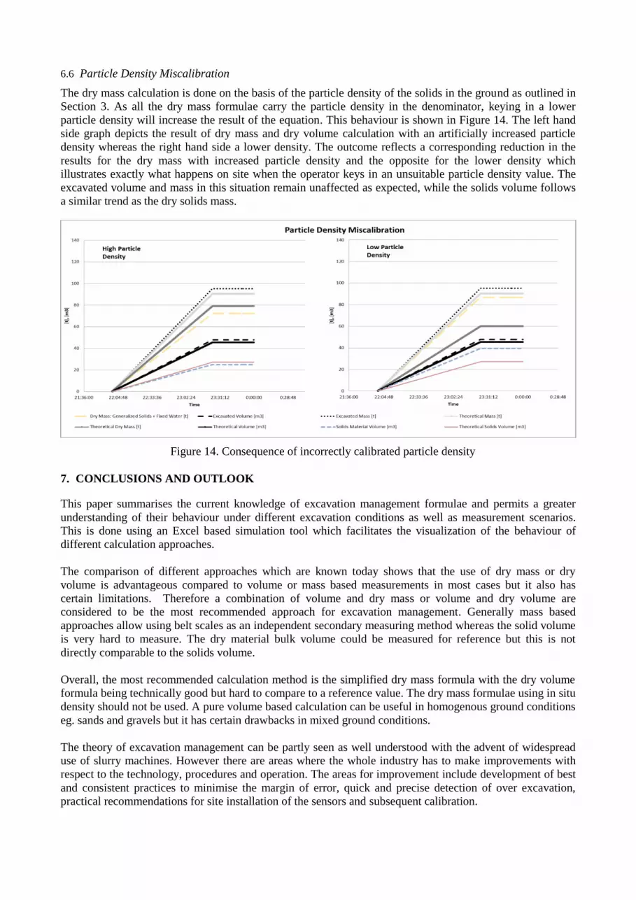
6.6 Particle Density Miscalibration

The dry mass calculation is done on the basis of the particle density of the solids in the ground as outlined in

Section 3. As all the dry mass formulae carry the particle density in the denominator, keying in a lower

particle density will increase the result of the equation. This behaviour is shown in Figure 14. The left hand

side graph depicts the result of dry mass and dry volume calculation with an artificially increased particle

density whereas the right hand side a lower density. The outcome reflects a corresponding reduction in the

results for the dry mass with increased particle density and the opposite for the lower density which

illustrates exactly what happens on site when the operator keys in an unsuitable particle density value. The

excavated volume and mass in this situation remain unaffected as expected, while the solids volume follows

a similar trend as the dry solids mass.

Figure 14. Consequence of incorrectly calibrated particle density

7. CONCLUSIONS AND OUTLOOK

This paper summarises the current knowledge of excavation management formulae and permits a greater

understanding of their behaviour under different excavation conditions as well as measurement scenarios.

This is done using an Excel based simulation tool which facilitates the visualization of the behaviour of

different calculation approaches.

The comparison of different approaches which are known today shows that the use of dry mass or dry

volume is advantageous compared to volume or mass based measurements in most cases but it also has

certain limitations. Therefore a combination of volume and dry mass or volume and dry volume are

considered to be the most recommended approach for excavation management. Generally mass based

approaches allow using belt scales as an independent secondary measuring method whereas the solid volume

is very hard to measure. The dry material bulk volume could be measured for reference but this is not

directly comparable to the solids volume.

Overall, the most recommended calculation method is the simplified dry mass formula with the dry volume

formula being technically good but hard to compare to a reference value. The dry mass formulae using in situ

density should not be used. A pure volume based calculation can be useful in homogenous ground conditions

eg. sands and gravels but it has certain drawbacks in mixed ground conditions.

The theory of excavation management can be partly seen as well understood with the advent of widespread

use of slurry machines. However there are areas where the whole industry has to make improvements with

respect to the technology, procedures and operation. The areas for improvement include development of best

and consistent practices to minimise the margin of error, quick and precise detection of over excavation,

practical recommendations for site installation of the sensors and subsequent calibration.

Detailed knowledge of the geomechanical processes and flows during face collapses or over-excavation

would greatly improve the possibility for early detection of such events based on the results of data analysis.

This can be complemented by large scale study of the sensor accuracy, the repeatability of the measurements

through effective calibration and increased knowledge on the uncertainty in measurements. With these steps

the Authors believe the industry will soon benefit from a more reliable and effective excavation management

system for slurry machines.

REFERENCES

[1] ASTM D4254, Standard Test Methods for Minimum Index Density and Unit Weight of Soils and

Calculation of Relative Density, ASTM International, West Conshohocken, PA, 2014.

[2] Bartlett, J. V., Biggart, A. R., Triggs, R. L., (1974) Bentonite Tunnelling Machine, Proceedings of the

Institution of Civil Engineers, Part 1, 7670, UK.

[3] Berthold Technologies (2015). Density Meter LB 444, Berthold Technologies GbmH & Co. KG, USA.

[4] Bochon, A., Rescamps, Y., Chantron, L. (1997). Detecting Anomalies During Slurry Shield Excavation:

Method Applied on EOLE site, France.

[5] BTS/ICE (2005). Closed-face Tunnelling Machines and Ground Stability: A Guideline for Best Practice.

British Tunnelling Society with the Institution of Civil Engineers, Thomas Telford, 77 p.

[6] DAUB (2006). Recommendations for Design and Operation of Shield Machines, German Committee for

Underground Construction Inc. (DAUB), Tunnel 6/2000, Germany.

[7] DIN 18 123 (1983). Baugrund; Untersuchung von Bodenproben; Bestimmung der Korngrößenverteilung,

Hrsg. Deutsches Institut für Normung, Beuth Verlag, Berlin.

[8] DIN 18 125 (1986). Baugrund; Bestimmung der Dichte des Bodens; Teil 1: Laborversuche, Hrsg.

Deutsches Institut für Normung, Beuth Verlag, Berlin.

[9] Duhme, R. (2015). Excavation Management in Slurry TBMs- Theoretical Foundations and Practical

Challenges, TUCSS Tunneling Course 2015, Tunnel and Underground Construction Society Singapore

[10] Duhme, R. (2015). Apparatus for Driving a Tunnel, Singapore Patent Application Number:

10201502431W (DE 102014104580.7)

[11] Earthnix Corporation (2014). On-line Density Meters GD-8000 Operation Manual, Earthnix

Corporation, Tokyo, Japan.

[12] Eichler, K. (2007). Fels- und Tunnelbau II, Expert Verlag, Renningen, Germany.

[13] Endress + Hauser (2007). Proline Promag 55 Electromagnetic Flow Measuring System,

BA119D/06/en/11.0, Endress + Hauser , Germany.

[14] Endress + Hauser (2007). Liquicap M FMI51, FMI52 Capacitance level measurement for continuous

measurement in liquids, TI00401F/00/en, Endress + Hauser , Germany.

[15] Golder Associates (2009). GeoReport No. 249, Ground Control for Slurry TBM Tunnelling. Hong

Kong.

[16] Guglielmetti, V. (2007). Process Control in Mechanized urban tunneling, Mechanized Tunneling in

Urban Areas. Design Methodology and Construction Control.

[17] Japan Society of Civil Engineers. (1984). Thesis Report No. 343, Tokyo, Japan.

[18] Maidl, B., Herrenknecht, M., Maidl, U., Wehrmeyer, G. (2001). Mechanised Shield Tunneling Ernst &

Sohn, Berlin.

[19] McChesney, S., Gasson, P., Nair, R. (2008). Slurry TBM Tunnelling Risk Control & Lessons learnt on

CCL Stage 4 – Contract 854, International Conference in Deep Excavations, Singapore.

[20] Nakano, A., Sahabdeen, M., Kulaindran, A., Seah, T. (2007). Excavation Management for Slurry TBMs

Tunnelling under Residential Houses at C853 (CCL3) Project, Underground Singapore 2007, Singapore.

[21] Ow, Chun Nam, Ariaratnam, K., Tiong Peng, S. (2007). Construction of Rail Tunnels Using Slurry

Machines on Circle Line Stage 3, Singapore, ACUUS Conference, Underground Space: Expanding the

Frontiers, Athens, Greece.

[22] Press, F., Siever R., (1985). Earth, W. H. Freeman and Company, New York.

[23] Rosenbusch, N. (2015). Mass Balance for Hydroshield TBM using Dry Mass Calculation and

IRIS.tunnel, ITC Advanced Engineering Asia Pte Ltd., Singapore.

[24] Rysdahl, B., Mooney, M., Grasmick, J. (2015). Calculation of Volume Loss using Machine Data from

Two Slurry TBMs during the Excavation of the Queens Bored Tunnels. Proc. Rapid Excavation and

Tunneling Conference 2015, New Orleans, USA

[25] Rysdahl, B., (2015). Determination of the Uncertainty in Excavated Volume Estimation from Slurry

Shield Tunnel Boring Machines used on the Queens Bored East Side Access Tunneling Project. Dissertation,

Colorado School of Mines, USA

[26] Sahabdeen, M., Kulaindran, A., Nakano, A. (2007). Dry Soil Volume for Excavation Management of

Slurry TBMs Tunnelling at C853 Project, Singapore, International Conference in Deep Excavations,

Singapore

[27] Shook, C.A., Roco, M.C., (1991). Slurry Flow- Principles and Practice, Butterworth Heinemann,

Boston, USA.

[28] Smoltczyk, U. (2002). Geotechnical Engineering Handbook Volume 1: Fundamentals, Ernst & Sohn,

Berlin, Germany.

[29] Uchida, Y., Ishiwata, K. (1977). Apparatus and Method of Shield Excavation, US Patent No. 4040666

[30] Wehrmeyer, G. (2000). Zur Kontrolle der geförderten Aushubmassen beim Tunnelvortrieb mit

Flüssigkeitsschilden, Dissertation, Ruhr University Bochum, Bochum

[31] Wehrmeyer, G. (2002). Massenkontrolle bei Schildvortrieben – Stand und Erfahrungen, Taschenbuch

Tunnelbau, VGE Verlag, Essen, Germany

[32] Wehrmeyer, G. (1999). Möglichkeiten der Aushubkontrolle bei Schildvortrieben, Bauingenieur Bd. 74

(1999) Nr. 2, Germany

[33] Yamazaki, H. (1983). Excavation Controlling Method in Hydraulic Shield Tunneling, US Patent No.

4384807

[34] Yamazaki, H. et al. (1984). Face Stability and Control of Excavation in the Shield Method, Journal

Report of Japan Civil Engineering Society 3/1984, Japan.

[35] Yamazaki, H. et al. (1976). Apparatus and Method of Measuring Fluctuations of Excavated Mud

Amount in a Slurry Line, US Patent No. 3946605.

[36] Yokogawa (2006). Magnetic Flowmeter ADMAG AXF, CA, Yokogawa Electric Corporation, Japan.

Documents

THEORETICAL BASIS OF SLURRY SHIELD EXCAVATION MANAGEMENT SYSTEMS