Doctoral Thesis in Material Science and Engineering

Thermodynamics and Kinetics in Metallurgical Processes - with a Special Focus on Bubble DynamicsYU LIU

Stockholm, Sweden 2020www.kth.se

ISBN 978-91-7873-714-7TRITA-ITM-AVL 2020:46

kth royal institute of technology

Yu Liu Therm

odynamics and Kinetics in M

etallurgical Processes - with a Special Focus on Bubble D

ynamics

KTH

2020

Thermodynamics and Kinetics in Metallurgical Processes - with a Special Focus on Bubble DynamicsYU LIU

Doctoral Thesis in Material Science and EngineeringKTH Royal Institute of TechnologyStockholm, Sweden 2020

Academic Dissertation which, with due permission of the KTH Royal Institute of Technology, is submitted for public defence for the Degree of Doctor of Engineering on Wednesday, December 16th, 2020, at 14:00 p.m. in Green room, Osquars backe 41, Stockholm.

© Yu Liu© Mikael Ersson, Pär Göran Jönsson, Björn Glaser ISBN 978-91-7873-714-7TRITA-ITM-AVL 2020:46 Printed by: Universitetsservice US-AB, Sweden 2020

To my beloved parents and wife Qiong Hou

送给我亲爱的父母和爱人侯琼

i

Abstract

Gas stirring is commonly used in the steelmaking processes to reinforce

chemical reactions, kinetic transfer, and inclusion removal, etc. This dissertation

concentrates on multiphase flows with gas bubbling to study fluid dynamics and

thermodynamics in metallurgical processes. A study of bubble behavior has been

carried out using a multiscale approach as follows: Prototype scale (macro) →

Plume scale → Single bubble scale → Reaction scale (micro).

Initially, previous works on physical modeling and mathematical modeling in

relation to the gas bubbling in the ladle have been reviewed. From that, several

aspects that can be improved were found:

For physical modeling, such as mixing and homogenization in ladles, the

general empirical rules have not been analyzed sufficiently;

The mathematical models focusing on inclusion behaviors at the steel-slag

interface need to be improved;

The phenomena governing the transfer of elements, vacuum degassing, and

the combination of fluid dynamics and thermodynamics, such as in desulfurization,

need to be investigated further.

The kinetics transfer with regards to temperature and element homogenization

is one of the most extensive research fields in steel metallurgy. For the analysis on

prototype scale, the optimal plug configuration has been studied for a 50t ladle. For

stirring using bottom-blowing, a separation angle between dual plugs of 160 degree

is mostly recommended, and the optimal dual-plug radial position is around 0.65R.

Moreover, the influence of the tracer’s natural convection on its homogenization

pattern cannot be neglected, especially for ‘soft bubbling’ conditions using low gas

flow rates.

Subsequently, in studies of the statistical behavior of gas bubbling in the plume,

mathematical modeling using an Euler-Euler approach and an Euler-Lagrange

approach have been compared. With respect to the bubble coalescence and breakup,

the Euler-Lagrange approach is more accurate in predicting the flow pattern for

ii

gas injection using a porous plug. With regards to the effect of plug design on

the statistical behavior of gas bubbling, gas injection using a slot plug promotes

kinetic reactions close to the open eye due to the concentrated plume structure,

and gas bubbling using a porous plug promotes a good inclusion removal

because of the increased amount of bubbles.

Focusing on single bubble behavior, under the same flow rate, as the top

gauge pressure is reduced, the bubble diameter increases and the bubble

generation frequency decreases. During the bubble ascent, a large bubble

gradually reaches stable conditions by means of shedding several small bubbles.

In a steel-argon system, under a flow rate in the range of 5.0(mL‧min-1)STP to

2000(mL‧min-1)STP, the bubble diameter is in the range of 6.0mm to 20.0mm.

Under laminar conditions, the maximum bubble width is 65mm when the

surrounding pressure is 0.2bar, and the steady bubble width is around 58mm

under a pressure of 2.0bar.

Finally, a coupling method, named Multi-zone Reaction Model, has been

developed to predict the conditions in the EAF refining process. Using a

combined injection of O2 and argon, and the same injected mass of O2, the

decarburization rate increases due to an efficient kinetic mass transfer of

carbon in the molten steel. Furthermore, using CO2 to replace argon, as the

ratio of the CO2 content in the injection increases, the maximum hot spot

temperature, the increment rate of average temperature, and the

decarburization rate decrease dramatically.

The research step from multiphase fluid dynamics to its coupling with high

temperature thermodynamics is a large advancement in this study. Moreover,

the research process using open source software to replace the commercial

software is also an important technical route. This can help the transparent

development of future modules for reacting flow in metallurgical processes.

Key words: ladle, EAF, gas bubbling, physical modeling, mathematical

modeling, thermodynamics

iii

Sammanfattning

Gasomrörning används frekvent inom järn och stålframställning för att

effektivisera kemiska reaktioner, kinetik, transport av inneslutningar osv. Denna

avhandling fokuserar på flerfasflöden med gasblåsning för att studera

fluidmekanik och termodynamik i metallurgiska processer. Avhandlingen

analyserar bubbelkaraktär i olika skalor: testugnsskala (makro) →

bubbelplymskala → enkelbubbelskala → jämviktsberäkningar (mikro).

Först och främst har metoderna för experimentell och matematisk modellering

av gas-bubblor i skänk från tidigare studier granskats. I dessa studier upptäcktes

följande svagheter:

Inom experimentell modellering av omrörning och homogenisering i

skänken har de generella empiriska reglerna inte analyserats tillräckligt utförligt;

De matematiska modellerna som fokuserar på inneslutningars beteende vid

stål-slagg gränsytan behöver förbättras;

Fenomen som styr transport av ämnen, vakuumavgasning, samt

kombinationen av fluidmekanik och termodynamik så som i svavelrening kräver

ytterligare forskning.

Ett av de mest omfattande forskningsfälteten inom metallurgi är kinetik som

styr temperatur och homogenisering av ämnen. I en analys i testugnsskala har den

optimala konfigurationen av porösa dysor studerats för en 50 ton skänk. Vid

bottenblåsning med två dysor rekommenderas en separationsvinkel på 160 grader

med en radiell positionering på 0.65R. Det upptäcktes även att effekten av den

naturliga konvektionen hos spårämnet inte kan försummas vid

homogeniseringsexperiment, speciellt vid låg flödeshastighet.

I studien av det statistiska beteendet hos bubbelplymen jämfördes två

numeriska metoder, Euler-Euler och Euler-Lagrange. Med hänsyn till

bubbelkoalescens och delning är Euler-Lagrange metoden mer precis för att

karakterisera flödet vid gasinjektion med porös dysa. Experimentell modellering

utfördes för att undersöka effekten av dysans design på bubblorna i plymen där

skillnaden mellan porös plug och ”slot” dysa studerades. Gas injektion med ”slot”

iv

dysa ökar kinetiken för reaktion nära ”open eye” området på grund av den

koncentrerade plymen. Däremot är gasblåsning genom en porös dysa mer

effektiv på att driva upp inneslutningar på grund av den större mängden

bubblor.

I studien på enkelbubblans beteende har effekten av nedsatt tryck vid

vattenytan på bubbel-bildning och uppstigning undersökts. Med samma

gasflöde och minskande tryck vid ytan ökar bubbeldiametern samtidigt som

bubbelfrekvensen minskar. När en stor bubbla stiger når den gradvis ett stabilt

läge genom att separera flera små bubblor från botten av bubblan. I ett system

av stål och argon är bubblans originaldiameter mellan 6.0mm och 20.0mm när

ett flöde mellan 5.0(mL‧min-1)STP och 2000(mL‧min-1)STP används. Under

laminärt tillstånd och ett tryck på 0.2bar är bubblans maximala bredd 65mm

och vid ett tryck på 2.0bar är bubblans stabila bredd ca 58mm.

Slutligen har en kopplingsmodell kallad ’Multi-zone Reaction Model’

utvecklats för att studera raffinering i en EAF process. En gasinjektion

bestående av O2 gas utspädd med inert argongas ökar kolfärskningshastigheten

på grund av en mer effektiv kinetisk masstransport av kol i smältan, jämfört

med samma injektionsmängd av enbart syrgas. Vidare, när argon byts mot CO2

och förhållandet av CO2 mot O2 ökar, minskar den maximala ’hot spot’

temperaturen och den genomsnittliga temperaturökningen samt hastigheten

för kolfärskningen dramatiskt.

Kopplingen mellan fluiddynamik och termodynamik är ett stort framsteg

som gjorts i denna studie. Dessutom har användningen av ’Open-source’

mjukvaror för att ersätta kommersiella mjukvaror varit en viktig del i arbetet

för att förstå numerisk fluiddynamik mer djupgående, modifiera variabler i

olika modeller och designa en mer precis modell för att undersöka

gasbubblornas beteende i metallurgiska processer.

Nyckelord: Skänkmetallurgi, EAF, gasbubblor, experimentell modellering,

matematisk modellering, termodynamik

vi

Acknowledgement

I would like to express my deepest gratitude to my supervisor Associate Professor

Mikael Ersson for his innovative ideas, patient guidance, and energetic

encouragement for my work and life. The spirit will always inspire me to overcome

the difficulties in my future research. I would like to express my respect to my co-

supervisor Professor Pär Jönsson for his in-deep knowledge, wisdom, and his

guidance to broaden my scope of knowledge. I would like to express my

appreciation to my co-supervisor Associate Professor Björn Glaser for his help for

the industrial experiences and support whenever I needed. His spirit of

hardworking silently influences me. Without their unending support and help, this

work would not be possible to complete.

Great thanks to Professor Yong Gan and Professor Heping Liu in Central Iron and

Steel Research Institute in Beijing, China. Great thanks to them for support and

help.

Thanks to Nils Å.I. Andersson, Dongyuan Sheng and Lars Höglund for discussion

and suggestions for my work on code compiling. Thanks to Christopher Hulme-

Smith for writing improvement.

Special thanks to Professor Dr.-Ing. Herbert Köchner (FOM Hochschule) for his

help and delightful discussion. Professor Dr.-Ing. Hans-Jürgen Odenthal (SMS

group GmbH) and Tim Haas (RWTH Aachen University) are acknowledged for

their help and suggestions to set up the water experiment.

I have learnt a lot of fundamental CFD knowledge from every week’s CFD meeting

organized by Mikael Ersson. The discussions are very helpful and interesting.

Thanks to graduated and current members in the CFD Group for their help to

discuss the CFD knowledge, to setup the experiment, and to internally review the

manuscripts.

vii

Thanks to my colleagues and friends in the MSE Department. The sport time in

each Thursday afternoon to play ‘Innebandy’ is the funniest moment to relax in

each week.

Special thanks to the financial support of CSC (China Scholarship Council) for my

study in Sweden. The research leading to the presented results has received funding

from the European Union’s Research Fund for Coal and Steel (RFCS) research

program under grant agreement N754064. Special thanks for this support.

Thanks to my friends met in Stockholm. Your companion, laughter and care in my

life is like the sunshine in the winter.

Finally, thanksgiving to my beloved parents and wife Qiong Hou for their endless

understanding and love. Your love is the source of my forward progress.

Yu Liu

Stockholm, 2020

viii

Supplements

The present thesis is based on the following supplements:

Supplement Ⅰ:

Supplement Ⅱ:

Supplement Ⅲ:

Supplement Ⅳ:

Supplement Ⅴ:

Supplement Ⅵ:

A Review of Physical and Numerical Approaches for the Study of Gas

Stirring in Ladle Metallurgy

Y. Liu, M. Ersson, H. Liu, P. G. Jönsson, Y. Gan

Metall. Mater. Trans. B, 2018, vol. 50B, pp. 557-577.

Physical and Numerical Modeling on the Mixing Condition in a 50 t

Ladle

Y. Liu, H. Bai, H. Liu, M. Ersson, P. G. Jönsson, Y. Gan

Metals, 2019, vol. 9, issue 11, no. 1136.

Comparison of Euler-Euler Approach and Euler–Lagrange

Approach to Model Gas Injection in a Ladle

Y. Liu, M. Ersson, H. Liu, P. G. Jönsson, Y. Gan

Steel Res. Int., 2019, vol. 90, no. 1800494.

Influence of Plug Design on Bubble Injection Characteristics in Ladle

Metallurgy

Y. Liu, M. Ersson, H. Liu, Y. Gan, P. G. Jönsson

In manuscript

An Experimental and Mathematical Work on Single Bubble Behavior

under Reduced Pressure

Y. Liu, M. Ersson, C. Hulme-Smith, H. Liu, P. G. Jönsson

In manuscript

Decarburization in an Electric Arc Furnace using Coupled Fluid

dynamics and Thermodynamics

Y. Liu, M. Ersson, B. Glaser, N. Å.I. Andersson, P. G. Jönsson

In manuscript

ix

Contribution to the supplements:

Supplement Ⅰ: Literature review and major part of this writing.

Supplement Ⅱ, Ⅲ, Ⅳ, Ⅴ, Ⅵ: Literature review, experimental work, numerical

simulation and major writing of the manuscript.

x

Contents

Abstract .................................................................................................................... i

Sammanfattning .................................................................................................... iii

Acknowledgement ................................................................................................. vi

Supplements ......................................................................................................... viii

Chapter 1 Introduction .......................................................................................... 1

1.1 Research background ......................................................................................................... 1

1.2 Literature review ................................................................................................................ 3

1.3 Aim of dissertation ............................................................................................................. 8

Chapter 2 Mathematical Modeling ...................................................................... 11

2.1 Numerical Assumptions ................................................................................................... 11

2.1.1 Supplement Ⅱ, Supplement Ⅲ & Supplement Ⅳ ..................................................... 11

2.1.2 Supplement Ⅴ ............................................................................................................ 11

2.1.3 Supplement Ⅵ ........................................................................................................... 11

2.2 Computational Fluid Dynamics (CFD) Model ................................................................ 11

2.2.1 Compressible ideal gas law ....................................................................................... 11

2.2.2 VOF Approach (VOF model and compressibleInterFoam) ...................................... 12

2.2.3 Euler-Euler Approach (Eulerian multiphase model and multiphaseEulerFoam) ...... 13

2.2.4 Euler-Lagrange Approach (Discrete Phase Model and Lagrangian) ......................... 15

2.2.5 The Turbulence Model .............................................................................................. 17

2.3 Thermodynamics Model .................................................................................................. 17

2.4 Boundary Conditions and Solution Methods ................................................................... 18

Chapter 3 Experimental Methodology ................................................................ 21

3.1 Scaling Criterion .............................................................................................................. 21

3.2 Experimental Apparatus ................................................................................................... 22

Chapter 4 Results and discussion ........................................................................ 25

xi

4.1 Physical and Numerical Modeling of the Mixing Condition in a 50t Ladle (Supplement

Ⅱ) ............................................................................................................................................ 25

4.2 Comparison of Euler-Euler Approach and Euler–Lagrange Approach for Gas Injection in

a Ladle (Supplement Ⅲ) ........................................................................................................ 32

4.3 Influence of Plug Design on the Bubble Injection Characteristics (Supplement Ⅳ) ...... 35

4.4 An Experimental and Mathematical Work on Single Bubble Behavior under Reduced

Pressure (Supplement Ⅴ) ........................................................................................................ 38

4.5 Decarburization in an Electric Arc Furnace using Coupled Fluid dynamics and

Thermodynamics (Supplement Ⅵ) ........................................................................................ 42

Chapter 5 Conclusions ......................................................................................... 47

Chapter 6 Sustainability and Recommendations for Future Work ................... 53

6.1 Sustainability .................................................................................................................... 53

6.2 Recommendation for Future Work .................................................................................. 53

References ............................................................................................................. 55

1

Chapter 1 Introduction

1.1 Research background

Steel is a metallic material which is extensively used, especially in industrial

engineering. With the development of industrial manufacturing, the process of

steelmaking has become mature. Simultaneously, the customer requirement for

cleaner steel with better quality has increased. From the 60th in the last century, a

fundamental change of the traditional oxygen steelmaking has taken place, and the

application of secondary refining process and the electric arc furnace (EAF) has

become widespread. The main metallurgical processes of steel manufacturing are

shown in Figure 1. The secondary refining processes, such as LF and RH, can

enable adjustments of the temperature and steel composition to improve the quality

of the final steel products. Moreover, in consideration of production efficiency and

economic benefit, the refining process can optimize the production logistics by

acting as a bridge between steelmaking and casting process steps.

Due to global problems of air pollution and the greenhouse effect caused by

CO2 emission, energy savings and environmental related process improvements

have become worldwide focus areas, which puts a demand on the steelmaking

industry. However, on the upside, with an increasing of scrap amount and the

development of new steelmaking processes, in comparison to the traditional ore-

based BOF process, the scrap-based EAF process is more efficient and

environmentally friendly.

2

Figure 1. Process of steel metallurgy (Reproduced by Ref.[1])

Gas bubbling is a widespread method in steelmaking processes to improve

homogenization and stirring of melts. In BOF and EAF processes, the oxygen

injection is employed to refine the iron melt through chemical reactions such as

decarburization and dephosphorization. In the ladle refining process, argon

bubbling is used to homogenize chemical compositions and temperature, to

enhance the kinetics for the reactions at the steel-slag interface, to remove non-

metallic inclusions, and to lower the contents of nitrogen and hydrogen. However,

if the gas injection isn’t controlled and used properly, severe problems can occur.

For example, using top lance oxygen jetting in the EAF process, the gas penetration

length is short and the oxygen just exists in the melt for a short time. Therefore,

there is a large amount of oxygen lost to the atmosphere during top lance oxygen

jetting, as shown in Figure 2(a). In recent years, the bottom-blown oxygen

injection has been applied in the EAF process. Nevertheless, the bottom blowing

is tough to control to prevent iron oxidation and to keep high metallic yields. Also,

if the argon stirring during ladle refining is overly strong, an open eye enlarges and

the steel-slag interface fluctuates severely. Thus, there is a high probability of

reoxidation of the clean steel and entrapment of large size inclusions from slag into

the molten steel, as shown in Figure 2(b). Therefore, the optimized and controlled

gas bubbling is of significant importance in steelmaking processes.

3

(a) (b)

Figure 2. Oxygen lance injection in an EAF (a) and open eye formation

by argon bubbling in a ladle (b) (Figure 2(a) is reproduced by Ref.[2])

1.2 Literature review

A large number of articles have been published to study gas stirring in

steelmaking processes. Both mathematical models and physical models have been

used separately or together according to the specific research focus to describe the

stirring processes. Argon bubbling in typical ladle refining processes contain most

of the gas injection functions in metallurgical processes, and the studies on argon

bubbling are most abundant and comprehensive.[3-7] Therefore, the existing

analysis of the mathematical modeling and physical modeling on ladle metallurgy

have been reviewed.[8]

Depending on specific research goals, previous lab-scaled physical modeling

experiments have been classified based on four major research areas: ⅰ) mixing and

homogenization in the ladle,[9-22] ⅱ) bubble formation, transformation, and

interactions in the plume zone,[23-53] ⅲ) inclusion behaviors,[17, 54-64] and ⅳ) steel-

slag interface behavior and open eye formation.[16, 20, 58, 65-83] Several industrial trials

have focused on open eye formation and the optimization of gas stirring. The

general empirical rules have not been analyzed sufficiently with respect to physical

modeling, such as mixing and homogenization in ladles. Moreover, the connection

4

between industrial trials and physical modeling experiments is essential for

determining scaling criteria. Froude similarity and modified Froude similarity

seem to be the most common dimensionless numbers used in gas-stirred

metallurgical reactors. The parameters of the water model, prototype, and

industrial ladles (that is, the gas flow rate, void fraction, plume radius, plume

velocity, and mixing time) are directly linked by the ratios of geometric factors or

transferred to dimensionless patterns first and then mathematically related.

In the existing mathematical modeling studies, four main mathematical models

have been used in different research fields to describe the bubble behavior and two-

phase plume structure: ⅰ) the quasi-single phase model,[23, 84-95] ii) the VOF

model,[49, 50, 96-109] iii) the Euler-Euler approach (Eulerian multiphase model),[13, 17,

55, 110-144] and ⅳ) the Euler-Lagrange approach (Eulerian-Lagrangian model).[15, 46,

94, 145-153] During the last years, the Euler-Euler approach and Euler-Lagrange

approach have been commonly used to predict the gas stirring conditions in the

metallurgical processes. Specific models in commercial packages or research

codes have been well developed to describe the complicated physical and chemical

phenomena step by step. The stirring dynamic given by gas bubbling crucially

influences flow patterns and its effects on the inclusion behavior, species transport,

and open eye formation. Therefore, it is meaningful to clarify the flow pattern to

prepare for further analysis on the thermodynamics phenomena. The physical

model experiments and numerical models to study the gas stirring in the ladle

process have classified and summarized in Figure 3, but detailed information is

given in Supplement I.

5

Figure 3. Schematic diagram of preferred numerical models in research directions

on ladle metallurgy

Based on the review of ladle refining processes, the following

recommendations regarding model combinations are suggested: ⅰ) for physical

modeling, such as mixing and homogenization in ladles, the general empirical rules

have not been analyzed sufficiently; ⅱ) the mathematical models focusing on

inclusion behaviors at the steel-slag interface need to be improved; and ⅲ) the

phenomena governing the transfer of elements, vacuum degassing, and the

coupling of fluid dynamics and thermodynamics, such as in desulfurization, need

to be further developed.

With the development of the computational capability, the modeling to predict

complicated thermodynamics phenomena in the multiscale with the fluid dynamics

has become feasible. In terms of the coupling of computational fluid dynamics and

thermodynamics using commercial softwares, several studies on the steelmaking

processes have been reviewed in Table 1. Ersson et al.[96] used the coupling method

6

of fluid dynamics and thermodynamics to study the decarburization rate, oxygen

content, and temperature distribution in a top-blown convertor. With consideration

of the metal-slag reactions, Ek et al.[154] developed the coupling method to predict

the mass transfer of carbon and phosphorus in the BOF converter process. In the

works of Andersson et al.[155-158], the effects of steel-slag interfacial reactions and

temperature on the decarburization and chromium oxidation conditions in the AOD

converter were investigated comprehensively. In terms of the prediction of

desulfurization in the ladle metallurgy, Jönsson et al.[159-161] developed an earlier

equilibrium model combined with a CFD multiphase model and focused on the

desulfurization reaction at the steel-slag interface, iron reoxidation, and aluminum-

silicon-manganese metallic elements equilibrium content in the melt. Considering

the thermodynamics reactions at the steel-slag interface and near the open-eye, Lou

and Zhu[135, 139] proposed a coupling method of CFD with the Simultaneous

Reaction Model in the gas-stirred ladle. Based on the Thermo-Calc database to

determine the solubility limit thermodynamic equilibrium composition between

steel and slag, Singh et al.[106] set up the coupling method with own code to predict

the desulfurization kinetics more computational efficiently. Also, Cao et al.[143]

established the thermodynamics database using Microsoft Excel worksheets to

couple with CFD model and predicted the desulfurization kinetics in the gas-stirred

ladle. In the works of Yu et al.[132, 137, 140], the coupling approach of CFD with an

own code was employed to predict the dehydrogenation and denitrogenation in the

vacuum degassing process. In Karouni et al.[144] work, the hydrogen removal rate

under an optimal plug configuration in the vacuum arc degasser was reported.

Moreover, Wang et al.[162-164] studied the macro-segregation, carbon, sulfur,

oxygen, and nickel contents of the alloy ingot during the electroslag remelting

(ESR) process including the coupled effect of electromagnetism on the multiphase

flow field.

7

Table 1. Coupling of fluid dynamics and thermodynamics using the commercial software

Author Year Process

Fluid

Dynamic

Model

Thermodynamics

Model Remarks

Jonsson

et al.[159] 1998 CAS-OB Phoenics own code Sulfur Refining

Andersson

et al.[160] 2000 Ladle Phoenics own code

Reoxidation and

Desulphurisation

Ersson

et al.[96] 2008 BOF Fluent Thermo-Calc Decarburization

Al-Harbi

et al.[165] 2010 Ladle Fluent MTDATA

Mass concentration of

the elements

(Al, O, and S)

Andersson

et al.[155-158, 161]

2012-

2013 AOD Phoenics Thermo-Calc

Decarburization and

chromium oxidation

Ek et al. [154]

2013 BOF COMSOL

Multiphysics own code

Mass transfer of

carbon and phosphorus

Yu et al. [132, 137, 140]

2013-

2015 VD

ANSYS

FLUENT own code

Dehydrogenation and

Denitrogenation

Lou and Zhu [135, 139]

2014-

2015 Ladle

ANSYS

FLUENT

own code

(Simultaneous

Reaction Model)

Thermodynamics

reactions at the steel-

slag interface and

nearby the open-eye

Singh et al. [106]

2016 Ladle ANSYS

FLUENT

own code+

Thermo-Calc

Desulfurization

kinetics

Wang et al. [162-164]

2016-

2018 ESR

ANSYS

FLUENT own code

Macro segregation and

element contents

Cao et al. [143]

2018 Ladle ANSYS

FLUENT

database in

Microsoft Excel

worksheets

Desulfurization

kinetics

Karouni

et al.[144] 2018 VD

ANSYS

FLUENT own code Hydrogen removal rate

8

1.3 Aim of dissertation

The aim of this thesis is to employ multiphase flow with gas bubbling to study

the fluid dynamics and thermodynamics in metallurgical processes. A schematic

diagram of the main work in this dissertation is shown in Figure 4. In supplement

Ⅰ, a review of the existing physical and numerical approaches to study gas stirring

in ladle metallurgy over last three decades is presented to give some options and

to find new and meaningful research directions. In supplement Ⅱ, physical

modeling to study the effect of plug configuration on the mixing condition was

carried out. The accuracy of developed mathematical models in the quasi-steady

mode and the transient mode was discussed. In supplement Ⅲ, the gas injection

using the porous plug in ladles was studied by using both the Euler-Euler approach

and the Euler-Lagrange approach. The effects of virtual mass force, turbulent

dispersion force, bubble sizes, and bubble injection frequencies on the flow pattern

were studied. In supplement Ⅳ, the statistic behaviors of gas bubbling, such as

plume width and periodic characteristics, were compared using a slot plug and

three porous plugs for gas injection. Moreover, the effects of plug porosity on the

plume width and average bubble size were studied using a physical model and a

mathematical model. In supplement Ⅴ, the generation and rising of single bubble

under reduced pressure was studied using a physical water model. A compressible

multiphase model was validated and used to predict the bubble behaviors in a steel-

argon system. Finally, in supplement Ⅵ, a coupling method of fluid dynamics and

thermodynamics, named as Multi-zone Reaction Model, was developed to predict

the decarburization process during the refining phase in the EAF furnace.

9

Figure 4. Schematic diagram of main work in this thesis

As shown in Figure 4, the study focuses on the bubble behaviors using a multi-

scale approach by considering from the prototype scale (macro) to the reactions

scale (micro). The combination of physical modeling and mathematical modeling

is a powerful and reliable method to predict unintuitive conditions in the

steelmaking processes.

11

Chapter 2 Mathematical Modeling

2.1 Numerical Assumptions

2.1.1 Supplement Ⅱ, Supplement Ⅲ & Supplement Ⅳ

Gas and liquid are incompressible Newtonian fluids;

The physical properties are constant;

The temperature is constant and no chemical reaction takes place in the

calculation system.

2.1.2 Supplement Ⅴ

The gas is treated as ideal gas, because the effect of pressure change has an

essential influence on the bubble behavior when it rises under the reduced

pressure condition;

The influence of the pressure change at different depths on the liquid is

neglected. So the parameters of liquid are constant;

The temperature is constant, and no chemical reaction takes place in the

calculation system;

No mass transfer of dissolved gas from the liquid into the bubble exists

during bubble formation and ascent.

2.1.3 Supplement Ⅵ

Gas and liquid are incompressible Newtonian fluids;

The physical properties are constant;

The temperature changes and equilibrium reactions take place in the

calculation system.

2.2 Computational Fluid Dynamics (CFD) Model

2.2.1 Compressible ideal gas law

According to the ideal gas law,

𝑝𝑉 = 𝑛𝑅𝑇 (1)

12

𝑝 is the absolute pressure of the ideal gas, 𝑉 is the volume of the gas, 𝑛 is the mole

of gas, 𝑅 is the ideal gas constant, 8.3144598J·K−1·mol−1, 𝑇 is the absolute

temperature of the gas.

If using the ideal gas law for compressible flow, the density is calculated as

follows:

𝜌𝑔𝑎𝑠 =𝑝𝑜𝑝+𝑝

𝑅

𝑀𝑇

(2)

where 𝑝𝑜𝑝 is the operation pressure (N·m-2), 𝑝 is the gauge pressure (N·m-2).

2.2.2 VOF Approach (VOF model and compressibleInterFoam)

The VOF model is widely used to track the interface of different phases, and it

belongs to the Eulerian method. When the flow rate is low, separate bubbles are

generated and the interfaces of different phases are sharp. In the VOF model, one

set of equations for continuity, momentum, and phase volume fraction is calculated.

The conservation formulas are shown as follows:

Continuity Equation:

𝜕𝜌

𝜕𝑡+ ∇ ∙ (𝜌�⃗� ) = 0 (3)

Momentum equation:

𝜕

𝜕𝑡(𝜌�⃗� ) + ∇ ∙ (𝜌�⃗� �⃗� ) = −∇𝑝 + ∇ ∙ [(𝜇 + 𝜇𝑡)(∇�⃗� + ∇�⃗� 𝑇)] + 𝜌𝑔 + 𝐹𝑠 (4)

Volume fraction:

𝜕𝛼𝑞

𝜕𝑡+ �⃗� ∙ ∇𝛼𝑞 = 0 (5)

Σ𝛼𝑞 = 1 (6)

(𝑞 is the fluid phase, e.g. liquid and gas)

The density and viscosity of mixed fluid in each cell are as follows:

𝜌 = 𝛼𝑙𝜌𝑙 + (1 − 𝛼𝑙)𝜌𝑔 (7)

𝜇 = 𝛼𝑙𝜇𝑙 + (1 − 𝛼𝑙)𝜇𝑔 (8)

The density in the plume is 𝜌 = α𝑔𝜌𝑔 + α𝑙𝜌𝑙 and the recirculation zone is

treated as a liquid phase 𝜌 = 𝜌𝑙. 𝜌 is the fluid density (kg·m-3), 𝜌𝑙 and 𝜌𝑔 are the

13

liquid and gas density (kg·m-3), α𝑞 is the volume fraction of each phase, �⃗� is

velocity component of the fluid (m·s-1), 𝑔 is the acceleration of gravity (m·s-2), 𝑝

is static pressure (N·m-2), 𝜇 is liquid viscosity (kg·m-1·s-1), 𝜇𝑡 is the turbulent

viscosity (kg·m-1·s-1), 𝐹𝑠 is the source force (N·m-3).

Continuum surface force model (CSF model):

The surface tension force in the CSF model is expressed as follows:

𝐹𝐶𝑆𝐹 = 𝜎𝜌𝜅∇𝛼𝑙

0.5(𝜌𝑙+𝜌𝑔), 𝜅 = ∇ ∙ �̂�, �̂� =

�⃗�

|�⃗� |, �⃗� = ∇𝛼𝑔 (9)

where 𝐹𝐶𝑆𝐹 is the surface tension force (N·m-3), 𝜎 is the surface tension coefficient

(N·m-1), �⃗� is the volume fraction gradient, and 𝜅 is the curvature (m-2).

2.2.3 Euler-Euler Approach (Eulerian multiphase model and multiphaseEulerFoam)

In the Euler-Euler approach, multiple sets of equations of continuity,

momentum, turbulent energy and dissipation rate were calculated for each phase.

For a better description of plume structure, the effect of forces, such as the virtual

mass force, drag force, lift force and turbulent dissipation force were considered in

the momentum equation. Therefore, the following conservations were solved:

Continuity Equation:

𝜕

𝜕𝑡(𝛼𝑞𝜌𝑞) + ∇ ∙ (𝛼𝑞𝜌𝑞�⃗� ) = 0 (10)

(𝑞 = 𝑙 is the equation for liquid phase, 𝑞 = 𝑔 is the equation for gas phase)

Momentum equation:

𝜕

𝜕𝑡(𝛼𝑞𝜌𝑞�⃗� 𝑞) + ∇ ∙ (𝛼𝑞𝜌𝑞�⃗� 𝑞�⃗� 𝑞)

= −𝛼𝑞∇𝑝 + ∇ ∙ (𝛼𝑞(𝜇 + 𝜇𝑡)(∇�⃗� 𝑞 + ∇�⃗� 𝑞𝑇)) + 𝛼𝑞𝜌𝑔 + 𝐹 𝑑𝑟𝑎𝑔,𝑞 + 𝐹 𝑇𝐷,𝑞 + 𝐹 𝑣𝑚,𝑞 + 𝐹 𝑙𝑖𝑓𝑡,𝑞

(11)

Population Balance Model

Transport equation:

𝜕

𝜕𝑡(𝑛(𝑉, 𝑡)) + ∇ ∙ (�⃗� 𝑖𝑛(𝑉, 𝑡)) = 𝐵𝑎𝑔,𝑖 − 𝐷𝑎𝑔,𝑖 + 𝐵𝑏𝑟,𝑖 − 𝐷𝑏𝑟,𝑖 (12)

𝐵𝑎𝑔,𝑖 =1

2∫ 𝛺𝑎𝑔(𝑉 − 𝑉′, 𝑉′)

𝑉

0𝑛(𝑉 − 𝑉′, 𝑡)𝑛(𝑉′, 𝑡)𝑑𝑉′, 𝐷𝑎𝑔,𝑖 ∫ 𝛺𝑎𝑔(𝑉, 𝑉′)

∞

0𝑛(𝑉, 𝑡)𝑛(𝑉′, 𝑡)𝑑𝑉′

(13)

14

𝐵𝑏𝑟,𝑖 = ∫ 𝑝0

𝛺𝑉𝛺𝑏𝑟𝑛(𝑉′, 𝑡)𝑑𝑉′, 𝐷𝑏𝑟,𝑖 = 𝑔(𝑉)𝑛(𝑉, 𝑡) (14)

where V is the volume of bubble (m3), 𝐵𝑎𝑔,𝑖 and 𝐵𝑏𝑟,𝑖 are the birth term due to

aggregation and breakage, 𝐷𝑎𝑔,𝑖 and 𝐷𝑏𝑟,𝑖 are the death term due to aggregation

and breakage, respectively.

The Luo Aggregation Kernel[166] was used to calculate the collisions of bubbles

with volumes 𝑉𝑖 and 𝑉𝑗:

𝛺𝑎𝑔(𝑉𝑖 , 𝑉𝑗) = 𝜔𝑎𝑔(𝑉𝑖 , 𝑉𝑗)𝑃𝑎𝑔(𝑉𝑖 , 𝑉𝑗) (m3/s) (15)

where 𝜔𝑎𝑔 is the frequency of collision and 𝑃𝑎𝑔 is the probability that the collision

results in coalescence.

𝜔𝑎𝑔(𝑉𝑖 , 𝑉𝑗) =𝜋

4（𝑑𝑖 + 𝑑𝑗）

2

�̅�𝑖𝑗 (16)

where �̅�𝑖𝑗 is the characteristic velocity of collision of two bubbles with diameters

𝑑𝑖 and 𝑑𝑗.

�̅�𝑖𝑗 = (�̅�𝑖2 + �̅�𝑗

2) (17)

where

�̅�𝑖 = 1.43(𝜀𝑑𝑖)1/3 (18)

The expression for the probability of aggregation is:

𝑃𝑎𝑔(𝑉𝑖 , 𝑉𝑗) = exp {−𝑐1[0.75(1+𝑥𝑖𝑗

2 )(1+𝑥𝑖𝑗3 )]

1/2

(𝜌2𝜌1

+0.5)1/2(1+𝑥𝑖𝑗)3

𝑊𝑒𝑖𝑗1/2

} (19)

where 𝑐1 is a constant of order unity, 𝑥𝑖𝑗 = 𝑑𝑖 𝑑𝑗⁄ , 𝜌1 and 𝜌2 are the densities of

the primary and secondary phases, respectively, and the Weber number is defined

as:

𝑊𝑒𝑖𝑗 =𝜌𝑙𝑑𝑖(𝑢𝑖𝑗)

2

𝜎 (20)

The Luo Breakage Kernel[167] was used to calculate the breakup of bubbles with

volumes 𝑉𝑖 and 𝑉𝑗:

𝛺𝑏𝑟 = 𝑔(𝑉′)𝛽(𝑉|𝑉′) = 0.9238𝛼(𝜀

𝑑2)1/3 ∫

(1+𝜉)2

𝜉𝑛

1

𝜉𝑚𝑖𝑛exp (−𝑏𝜉𝑚)𝑑𝜉 (21)

15

𝜉 = 𝜆/𝑑 is the dimensionless eddy size.

2.2.4 Euler-Lagrange Approach (Discrete Phase Model and Lagrangian)

In the discrete phase model, the forces, such as virtual mass, buoyancy, drag

force, lift force and pressure gradient, are added on each bubble particle optionally.

The momentum source term is added to the continuous phase momentum by

summing the local contributions from each bubble in the continuous phase flow

field. The forces on the bubble particles are calculated as follows:

𝑑�⃗⃗� 𝑏𝑖

𝑑𝑡=

�⃗⃗� −�⃗⃗� 𝑏𝑖

𝜏𝑟+

�⃗� (𝜌𝑏−𝜌)

𝜌𝑏+ 𝐹 𝑜𝑡ℎ𝑒𝑟 (22)

𝜏𝑟 =𝜌𝑏𝑑𝑏𝑖

2

18𝜇

24

𝐶𝐷𝑅𝑒 (23)

𝐹𝑏𝑖 = ∑(𝐹 𝑑𝑟𝑎𝑔 + 𝐹 𝑏𝑢𝑜𝑦𝑎𝑛𝑐𝑦 + 𝐹 𝑜𝑡ℎ𝑒𝑟)�̇�𝑏∆𝑡 (24)

𝑢𝑏𝑖 and 𝜌𝑏 are the velocity and density of bubble particles respectively, 𝜏𝑟 is the

bubble relation time, 𝐶𝐷 is drag coefficient. Furthermore, 𝐹𝐷𝑖 is the drag force per

unit particle mass in each control volume, �̇�𝑏 is mass flow rate of bubble particles

through each control volume.

Standard Parcel Release Method

In this method, a single bubble parcel is injected per injection stream per time

step. The number of bubble particles in the parcel is determined as follows:

𝑁𝐵 = �̇�𝑠∆𝑡

𝑚𝑏 (25)

where 𝑁𝐵 is the number of bubble particles in a bubble parcel, �̇�𝑠 is the mass flow

rate of the bubble stream, ∆𝑡 is the time step, 𝑚𝑏 is the particle mass.

For the Euler-Lagrange approach, there is only one bubble particle in each

parcel is considered, so it means each parcel stands for a bubble.

Discrete Random Walk Model

In the Euler-Lagrange model, the discrete random walk model was used to

describe the interaction between bubble particles and turbulence eddies in the fluid

phase. The velocity fluctuation of eddies are treated as isotropic, so

𝑢𝑖 = �̅�𝑖 + 𝑢′ = �̅�𝑖 + 𝜁√2𝑘/3 (26)

16

where 𝜁 is a normally distributed random number greater than 0 and less than 1.

The time scale can influence the lifetime of eddies to transfer momentum in

the plume zone indirectly. Therefore, the time scale influences the characteristics

of the plume. The plume's velocity distribution, the width of the plume, and bubble

particle behavior are considered when the turbulence coupling between the bubble

particles and liquid phase.

Collison and Discrete Coalescence Model

The O’Rourke’s algorithm[168] is used to calculate the bubble collision. The

mean characteristic number of collisions is calculated as follows:

�̅� =𝑛2𝜋(𝑟1+𝑟2)

2𝑣𝑣𝑒𝑙∆𝑡

𝑉𝑐𝑒𝑙𝑙 (27)

The probability distribution of collision follows a Poisson distribution,

𝑃(𝑛) = 𝑒−�̅� �̅�𝑛

𝑛! (28)

The critical offset is calculated as follows:

𝑏𝑐𝑟𝑖𝑡 = (𝑟1 + 𝑟2)√min (0.1,2.4𝑓

𝑊𝑒) (29)

where 𝑓 is defined as (𝑟1 𝑟2⁄ )3 − 2.4 ∗ (𝑟1 𝑟2⁄ )2 + 2.7 ∗ (𝑟1 𝑟2⁄ ), Weber number is

defined as 𝜌𝑢𝑟𝑒𝑙

2 �̅�𝑏

𝜎, 𝑢𝑟𝑒𝑙 is the relative velocity between two parcels, �̅�𝑏 is mean

diameter of two parcels. The actual value of collision 𝑏 is (𝑟1 + 𝑟2)√𝑌, where 𝑌 is

a random number between 0 and 1.

If 𝑏 < 𝑏𝑐𝑟𝑖𝑡, the result of collision is coalescence. Based on the conservation

of momentum and kinetic energy, the mass of new bubble is 𝑚 = 𝑚1 + 𝑚2, the

velocity of new bubble is 𝑣 =𝑚1𝑣1+𝑚2𝑣2

𝑚.

Otherwise, the result of collision is grazing collision, the bubble mass is

unaltered and the velocity updates to

𝑣𝑖′ =

𝑚𝑖𝑣𝑖+𝑚𝑗𝑣𝑗

𝑚𝑖+𝑚𝑗+

𝑚𝑗(𝑣𝑖−𝑣𝑗)

𝑚𝑖+𝑚𝑗(

𝑏−𝑏𝑐𝑟𝑖𝑡

𝑟1+𝑟2−𝑏𝑐𝑟𝑖𝑡) (30)

17

2.2.5 The Turbulence Model

In the Euler-Euler approach and Euler-Lagrange approach to predict the flow

pattern, the realizable k-ε model, which contains two equations of turbulence

kinetic energy k and its dissipation rate ε, was used to solve the turbulence

properties in the effective viscosity flow.

2.3 Thermodynamics Model

In the thermodynamics calculation, the TCFE10 (Steel/Fe-Alloys v10.1) and

SSUB6 (SGTE Substance Database, v6.0) were used to predict the equilibrium

conditions of elements in the liquid phase and species in the gas phase, respectively.

In order to communicate with the information between the fluid dynamics model

and the thermodynamics model, an application programming TQ interface

equipped with the Thermo-Calc software was used. The software interface between

the CFD-package and the thermodynamic databases was coded in C language. The

calculation mechanism of Multi-zone Reaction Model using thermodynamics

coupled to CFD and the solution procedure were shown in Figure 5.

Figure 5. Calculation mechanism of Multi-zone Reaction Model

Multiphase

Eulerian Model

(Liquid/Gas)

Multi-zone Reaction Model

Thermo-Calc

databases

Transport Description

Physics Parameters

Diffusion constant

Density

Viscosity

……

Output

18

2.4 Boundary Conditions and Solution Methods

The physical properties used in mathematical modeling were listed in Table 2.

The comparison of the calculation solver and solution method was illustrated in

Table 3. In the Euler-Euler approach, the outlet condition was set up as degassing,

which meant that dispersed gas bubbles were allowed to escape, and the continuous

liquid phase considered the boundary as a free-slip wall and could not leave the

domain; no-slip boundary condition was used at the wall; the inlet velocity

boundary condition was used to give a gas injection with a constant velocity; the

pressure-based solver was chosen to calculate the equations in the transient mode

to reach a quasi-steady state condition; the multiphase formulation was solved

implicitly with a coupled scheme. In the Euler-Lagrange approach, a pressure-

outlet condition was employed at the outlet boundary; no-slip boundary condition

was also used at the wall, but inlet boundary condition was used to inject bubble

parcels in DPM model; the pressure-based solver was chosen to solve the

multiphase formulations explicitly with a PISO scheme. In the calculation systems,

the commercial CFD package in ANSYS Fluent 2019 R3[169, 170] and the open

source CFD package OpenFOAM 7[171] were used to solve the governing equations.

The Eulerian Multiphase Model was used to calculate two sets of equations for the

gas and liquid phases in Eulerian coordinates. The Euler-Lagrange approach was

the coupling method of the Volume of Fluid Model (VOF model) and the Discrete

Phase Model (DPM). Specifically, the VOF model was used to track the interface

of different phases in the Eulerian coordinate system. The bubble particles were

tracked by the DPM model in the Lagrangian coordinate system.

19

Table 2. Physical properties used in the simulation

Parameter Physical Modeling Industrial

Water Air Argon Liquid steel Oxygen

Density

(kg·m-3) 998 1.225 1.62 7020 1.3

Dynamic viscosity

(kg·m-1·s-1) 0.001 1.79·10-5 8.9·10-5 0.0055 4.9·10-5

Specific heat

(J·kg-1·K-1) - - - 460 1150

Thermal conductivity

(W·m-1·K-1) - - - 64.4 0.045

Surface tension (N·m-1) 0.0728 1.82

Table 3. Boundary conditions in the models

Approach Euler-Euler Euler-Lagrange

Models Eulerian Multiphase

Model

Volume of Fraction

Model

Discrete Phase Model

Wall No-slip No-slip

Outflow Degassing Pressure-outlet

Solver type Pressure-based, Transient Pressure-based,

Transient

Formulation Implicit Explicit

Pressure-velocity coupling scheme Coupled PISO

Convergence criteria 10-4 10-4

Time step size (s) 10-4 10-4

21

Chapter 3 Experimental Methodology

3.1 Scaling Criterion

The connection between physical modeling experiments and industrial trials is

the scaling criterion. In this study, water and air, at room temperature, were used

to represent molten steel and argon, respectively. For the gas injection scaling, the

ratio of the inertial and buoyancy forces in the plume was considered to achieve a

flow similarity between the reactors. Using the geometric similarity ( 𝜆 =

𝐿𝑤𝑎𝑡𝑒𝑟 𝑣𝑒𝑠𝑠𝑒𝑙

𝐿𝑠𝑡𝑒𝑒𝑙 𝑙𝑎𝑑𝑙𝑒) and modified Froude number(𝐹𝑟𝑚 =

𝜌𝑔𝑎𝑠2 𝑄2

𝜌𝑙𝑖𝑞𝑢𝑖𝑑2 𝑔𝐻𝑑0

4),[172] the flow rates in

the prototype and water experiment can be correlated as follows:

𝑄𝑎𝑖𝑟 = (𝜌𝑎𝑟𝑔𝑜𝑛𝜌𝑤𝑎𝑡𝑒𝑟𝑑𝑤𝑎𝑡𝑒𝑟

2

𝜌𝑎𝑖𝑟𝜌𝑠𝑡𝑒𝑒𝑙𝑑𝑠𝑡𝑒𝑒𝑙2 √

𝐻𝑤𝑎𝑡𝑒𝑟

𝐻𝑠𝑡𝑒𝑒𝑙)𝑄𝑎𝑟𝑔𝑜𝑛

′ (31)

where 𝑑𝑤𝑎𝑡𝑒𝑟 is the plug diameter in the physical modeling, 𝑑𝑠𝑡𝑒𝑒𝑙 is the plug

diameter in the prototype, 𝜌𝑎𝑖𝑟 and 𝜌𝑤𝑎𝑡𝑒𝑟 are the densities of air and water,

𝜌𝑎𝑟𝑔𝑜𝑛 and 𝜌𝑠𝑡𝑒𝑒𝑙 are the densities of argon and steel, 𝐻𝑤𝑎𝑡𝑒𝑟 is the filled water

height, 𝐻𝑠𝑡𝑒𝑒𝑙 is the filled molten steel height, 𝑄𝑎𝑖𝑟 is the air flow rate in the

physical modeling (NL‧min−1), and 𝑄𝑎𝑟𝑔𝑜𝑛′ is the effective flow rate in the

prototype (NL‧min−1).

In several works,[20, 173] the effects of temperatures and pressures on the scaling

corrections were also studied. The temperature and pressure are taken into

consideration by using the ideal gas law 𝑝𝑣 = 𝑛𝑅𝑇 and 𝑝𝑖𝑛 = 𝑝0 + 𝜌𝑠𝑡𝑒𝑒𝑙𝑔𝐻𝑠𝑡𝑒𝑒𝑙,

respectively. Overall, the scaling criterion is derived as follows:

𝑄𝑎𝑖𝑟 = (𝜌𝑎𝑟𝑔𝑜𝑛𝜌𝑤𝑎𝑡𝑒𝑟𝑑𝑤𝑎𝑡𝑒𝑟

2

𝜌𝑎𝑖𝑟𝜌𝑠𝑡𝑒𝑒𝑙𝑑𝑠𝑡𝑒𝑒𝑙2 √

𝐻𝑤𝑎𝑡𝑒𝑟

𝐻𝑠𝑡𝑒𝑒𝑙)

𝑇𝑖𝑛

𝑇0∙

𝑝0

𝑝𝑖𝑛𝑄𝑎𝑟𝑔𝑜𝑛 (32)

where 𝑇0 is the normal temperature (273 K), 𝑇𝑖𝑛 is the molten steel temperature in

the prototype (1873 K), 𝑝0 is the atmospheric pressure (101325 Pa), 𝑝𝑖𝑛 is the

22

bottom injection pressure in the prototype (Pa), and 𝑄𝑎𝑟𝑔𝑜𝑛 is the flow rate under

normal conditions in the prototype (NL‧min−1).

3.2 Experimental Apparatus

The vessels in the physical experiments were made of transparent acrylic

plastic glass (PMMA). The compressed air was injected into water and its inlet

pressure and mass flow rate were adjusted by using a pressure controller and

an electric mass flow rate controller, respectively. For the vacuum bubbling, a

vacuum pump was connected to the vessel and a pressure gauge was installed

on the top of vessel to control the pressure inside the cylinder vessel. A high-

speed camera, connected to a computer to save data, was used to capture the

bubble behaviours. Note that, a strong LED light was preferred because the

camera was light sensitive. The experimental setups used in each supplement

were shown in Figure 6.

(a)

23

(b)

(c)

Figure 6. Experimental setups in each supplement study.

(a) Mixing condition, (b) Statistic analysis on bubbling,

(c) Single bubble behaviour under reduced pressure.

24

In supplement Ⅵ, the physical modeling was carried out to study the effect

of nozzle size on the flow field under the same flow rate. The experimental

apparatus was shown in Figure 7. A Met-Flow® Ultrasonic Velocity Profiling

(UVP) measurement,[174] equipped with a spatial resolution of 0.74 mm and

using a sampling rate of 19 ms, was used to determine the velocity pattern

along two lines (where the inside line was near the plume and the outside line

was near the side wall).

Figure 7. Experimental setup

(a) Real diagram of physical modeling, (b) Schematic diagram of physical modeling,

(c) UVP, (d) bottom nozzles with the inlet diameters of 10mm, 20mm, and 30mm.

In the industrial measurement, a thermocouple of DynTem[175], was used to

monitor the dynamic temperature at the hot spot zone. Moreover, the carbon

content in the molten steel was measured at the beginning and end points

during the refining phase.

(a) (b)

(c) (d)

25

Chapter 4 Results and discussion

4.1 Physical and Numerical Modeling of the Mixing Condition in a 50t Ladle

(Supplement Ⅱ)

The kinetics transfer with respect to temperature and element homogenization

is one of the most extensively research fields in steel metallurgy. The main studies

focusing on physical modeling and mathematical modeling began with the

determination of flow field and mixing conditions in the present work. The total

normalized conductivity curves using two probes in the physical modeling and

using eight points in the mathematical modeling were obtained, as shown in Figure

8(a) and 8(c). Moreover, the same conductivity curves with a specified range of

0.9 to 1.1 were shown in Figure 8(b) and 8(d), respectively. The solid and dashed

lines represent the tracer concentrations within ±5% and ±1% of homogenization

degrees’, respectively. For the ±5% homogenization degree case, the mixing time

was determined as the concentration of the tracer, which was continuously within

±5% of a well-mixed bulk value.[8] The procedure was the same for the case using

a ±1% homogenization degree, but the mixing time corresponded to a ±1% well-

mixed bulk value. The method to post-process the calculation data was the same

as that used to post-process the experimental results. The solid and dashed lines

correspond to the normalized mass fractions of tracers within the ±5% and ±1%

homogenization degrees, respectively.

26

(a) (b)

(c) (d)

Figure 8. Normalized conductivity curves determined using physical modeling and

mathematical modeling for a flow rate of 1.30NL·min−1

using a 135° plug separation angle.

(a) and (c) are normalized values with whole range in the physical modeling and

mathematical modeling; (b) and (d) are normalized values between 0.9 and 1.1 in the

physical modeling and mathematical modeling.

Concerning the effect of the tracer’s density on its homogenization pattern, the

conditions with and without fixed flow patterns were compared in the

mathematical modeling, as shown in Figure 9. The red and blue vectors

correspond to the convection pattern and the diffusion pattern, respectively. In

comparison to the species transport with and without fixed flow patterns, the

species transfer without fixed flow patterns agrees better with the physical

modeling results. Here, the effect of the tracer’s density on its mixing pattern is

considered. The result shows that the influence of the alloy’s natural convection

27

on its homogenization pattern cannot be neglected, especially for ‘soft bubbling’

conditions, when low flow rates are used. In terms of the physical modeling, it is

complicated to relate the tracer’s density to the alloy’s density used in the industrial

process. Therefore, it could be more accurate if the mathematical modeling results

are validated with data from physical modeling experiments and thereafter are used

to predict the industrial conditions, instead of using physical modeling results to

directly predict industrial conditions.

(a)

(b) (c)

28

(d)

(e)

Figure 9. Effect of tracer’s natural convection on mixing pattern

for a low flow rate of 0.98NL‧min−1

(a) Color dye experiments, (b) Euler-Euler and (d) Euler-Lagrange approaches using fixed

flow patterns, (c) Euler-Euler and (e) Euler-Lagrange approaches using transient flow patterns.

The mixing times in the physical and mathematical modeling were collected in

Table 4. Due to the comparison, the mixing time predicted by the Euler-Lagrange

approach in a quasi-steady mode for each condition is always less than that

predicted by the physical modeling. Therefore, some parameters in the Euler–

Lagrange approach, such as the drag coefficient, need to be modified further.

Moreover, the main errors between physical modeling results and mathematical

modeling results exist when using the conditions of a low flow rate and the

separation angle of 90 degrees. In comparison to the mathematical modeling in the

29

Quasi-steady mode, the errors of mixing time using the Euler-Euler approach in a

transient mode decrease significantly. However, with the consideration of the

tracer’s natural convection caused by the density change, the errors between the

physical modeling and mathematical modeling results for higher flow rates are still

larger than 5%. Therefore, it is necessary to modify the model further.

Table 4. Comparison of mixing times between physical modeling

and mathematical modeling results

The bubble distribution and flow field in an industrial 50t ladle during the

bottom blowing using off-centered and dual plugs with a 90degree, a 135degree,

and a 180degree angles were shown in Figure 10, respectively. For the same total

flow rate, the volume ratio of gas phase at the central plume zone using an off-

centered plug blowing is twice as large as that using dual-plug blowing. Thus, the

average bubble size for the off-centered condition is assumed to be larger because

of the bubble interactions. Moreover, for the off-centered blowing, the flow field

violently circulates along the central axis of plug. With an increased plug

separation angle, the flow field changes from a one-circle pattern to a two-circle

pattern. For the off-centered blowing case, the eccentric circulating at the central

zone in the ladle is intense, and the flow field of side zone at the bottom is weak.

For the dual plug bottom blowing case, the intensity of circulating at the central

zone gradually is reduced with an increased angle. Thereafter, the flow field of side

zone at the bottom becomes strengthened.

Software and

Flow Field Bottom-blown

90degree

Bottom-blown

135degree

Bottom-blown

180degree

ANSYS

FLUENT

Flow Rate

(NL⋅min-1) Phy. Math. Error Phy. Math. Error Phy. Math. Error

Euler-Lagrange

Quasi-steady

0.98 66 129.3 96% 74 130.5 76% 62 111 79%

1.3 62 92.3 49% 65 68.7 6% 60 66.2 10%

1.63 57 82 44% 53 61 15% 57 60 5%

OpenFOAM Flow Rate

(NL⋅min-1) Phy. Math. Error Phy. Math. Error Phy. Math. Error

Euler-Euler

Transient

0.98 66 68 3% 74 78 5% 62 64 3%

1.3 62 60 3% 65 67 3% 60 58 3%

1.63 57 53 7% 53 52 2% 57 52 10%

*Bonds with the large error

30

(a) (b)

(c) (d)

Figure 10. Bubble distribution, flow field, and homogenization process in a 50t ladle

(a) Off-centered bottom blowing, (b) Dual plugs with 90degree,

(c) Dual plugs with 135degree, (d) Dual plugs with 180degree.

In the mathematical modeling, the mixing time was defined by the means of

that the average mass fraction stays within the ±5% range of a total homogenized

concentration. The mixing time was mainly dominated by the concentration of

monitoring points at the side-bottom zone, named the ‘Dead Zone’, in the ladle.

The mixing times predicted by the mathematical modeling in the 50t ladle were

compared in Figure 11. The prediction shows that the mixing time with the off-

centered blowing is largest, and the mixing time for a bottom blowing using a dual

plug decreases firstly and increases thereafter with an increased separation angle.

The shortest mixing time is found when using a configuration with a separation

angle of 160 degree and it has a value of approximately 101s.

Bubble Diameter

Bubble Diameter

Bubble

Diameter

Bubble

Diameter

31

Figure 11. Homogenization times for various injection configurations

For the ladles with various weights, the optimal radial positions and separation

angles of the plugs in previous works were collected, as shown in Figure 12. In

terms of the mixing condition, an optimal range of plug’s radial location is mainly

off-centered for a single plug injection for values ranging from 0.72R to 0.75R.

For dual-plug injections, a separation angle between the plugs of approximately

160° is mostly recommended, and the optimal dual-plug radial position is around

0.65R. Overall, larger radial angles in the range of 135~180° are recommended to

reach a bubbly stirring condition when using dual porous plugs.

Figure 12. Optimal radial positions and separation angles of plugs in ladles

with various weights

203s

158s

128s108s 101s

125s

0

50

100

150

200

250

Tim

e(s)

off-centered90 degree135 degree150 degree160 degree180 degree

32

4.2 Comparison of Euler-Euler Approach and Euler–Lagrange Approach

for Gas Injection in a Ladle (Supplement Ⅲ)

In the studies of the flow field and mixing conditions, it was found that the

selection of multiphase models have an essential influence on the simulation results.

Therefore, the main approaches, namely the Euler-Euler approach and the Euler-

Lagrange approach, to predict the multiphase flow should be compared in detail.

Furthermore, the bubble’s behaviors, such as collision, coalescence and breakup,

were also needed to be studied by the advanced sub-model in two approaches. For

the Euler-Lagrange approach, the relationship among the bubble injection

frequency, bubble diameter and bubble number per unit injection time were linked

and various bubble generation patterns were shown in Figure 13. The predicted

axial velocity was compared with experiment data[29] in Figure 14(a) and (b). For

the axial velocity, the comparison shows that the simulation result is consistent

with experiment data for different injection patterns. It is shown that the bubble

injection pattern does not have a critical influence on the velocity distribution at

the same flow rate, which is consistent with the experimental results from previous

studies.[23, 176]

33

Figure 13. Regime of discrete bubbles formed when injecting gas through porous plugs.

The experiments are reproduced with permission.[29]1990, Springer US.

(a) (b)

Figure 14. Velocity magnitude at different heights

(a) Velocity magnitude with various injection frequencies,

(b) Velocity magnitude with various bubble sizes.

In order to predict the bubble size distribution in the plume zone, for the flow

rates of 600(cm3⋅s-1)STP and 1200(cm3⋅s-1)STP, the gas volume fraction and the

probability of bubble size distribution predicted by the Population Balance Model

in OpenFOAM were shown in Figure 15, respectively. As the flow rate increases,

the gas volume fraction at the plume zone increases. For the bubble distribution,

A

B C

E D

Experime

nt

-0.3 -0.2 -0.1 0.0 0.1 0.2 0.3

-0.20.00.20.40.60.81.01.21.4

z380mm- experiment [29]

z380mm- A 100s-1

z380mm- B 200s-1

z380mm- C 1000s-1

-0.3 -0.2 -0.1 0.0 0.1 0.2 0.3

-0.20.00.20.40.60.81.01.21.4

z200mm-experiment [29]

z200mm-A 100s-1

z200mm-B 200s-1

z200mm-C 1000s-1

-0.3 -0.2 -0.1 0.0 0.1 0.2 0.3

-0.20.00.20.40.60.81.01.21.4

z200mm- experiment [29]

z200mm- A 2mm

z200mm- D 1mm

z200mm- E 4mm

-0.3 -0.2 -0.1 0.0 0.1 0.2 0.3

-0.20.00.20.40.60.81.01.21.4

z380mm- experiment [29]

z380mm- A 2mm

z380mm- D 1mm

z380mm- E 4mm

34

the bubbles with the smallest size of 2mm are mainly distributed at the fully

developed buoyancy zone and surface zone of the plume. Nevertheless, the bubbles

with larger sizes of 32mm are mainly distributed in the primary zone and transition

zone in the plume. For a flow rate of 600(cm3⋅s-1)STP, the average distribution’s

probabilities of 2mm and 32mm bubbles are 0.18 and 0.04, respectively. For a flow

rate of 1200(cm3⋅s-1)STP, the average distribution’s probabilities of 2mm and 32mm

bubbles are 0.12 and 0.1, respectively. It is shown that, as the flow rate is increased,

the probability to generate small bubbles is gradually reduced, and the probability

to generate large bubbles is gradually increased. These results are consistent with

previously reported experimental result.[29]

(a) (b)

(c) (d) (e) (f)

Figure 15. Gas volume fraction and probability of bubble size distribution under flow rates of

600(cm3⋅s-1)STP and 1200(cm3⋅s-1)STP

(a), (c), and (e) correspond to 600(cm3⋅s-1)STP flow rate;

(b), (d), and (f) correspond to 1200(cm3⋅s-1)STP flow rate.

35

4.3 Influence of Plug Design on the Bubble Injection Characteristics

(Supplement Ⅳ)

In the mathematical modeling to predict the bubble behaviors using the Euler-

Euler and Euler-Lagrange approaches, the bubble size should be determined by

using physical modeling. Here, several vital coefficients, such as the turbulent

dispersion, were still needed to be modified based on some certain conditions. In

this part, the statistic characteristic of gas bubbling were studied using physical and

mathematical modeling. For the bubble injection using slot plugs, the effect of flow

rate on the gas-liquid plume was shown in Figure 16. For a flow rate of 0.5NL⋅min-

1, the gas volume fraction in the gas-liquid flow is lower, and the gas distribution

in the plume corresponds to discrete bubbling condition. The bubble is relatively

sparse and its average size in the cap-shape is around 3.8mm. With an increased

flow rate, the average bubble size increases to a small extent and the quantity of

discrete bubbles gradually increases. For a flow rate of 1.5NL⋅min-1, a small

amount of bubbles begin to collide and thereby aggregate into bubble clusters.

When the flow rate increased to 2.0NL⋅min-1, a large quantity of discrete bubbles

collide and form large bubbles. As the flow rate is increased, the gas volume

fraction in the central plume gradually increases, but the width of the plume always

remain approximately constant. In order to study the gas-liquid flow using a porous

plug, the plug with a porosity of 30% was firstly employed, and the flow conditions

using various flow rates were compared, as shown in Figure 17. For a flow rate of

0.5NL⋅min-1, the gas volume fraction in the central plume is low, and the gas

distribution corresponds to dispersive bubbles. The average size of bubbles having

an ellipsoidal shape is around 1.9mm. With an increased flow rate, the average size

of bubbles increases to 2.8mm, and the amount of dispersive bubbles increases

significantly. When the flow rate is increased to 2.0NL⋅min-1, in the fully

developed buoyancy zone, a large amount of bubbles are still under the dispersive

condition and only a few large bubbles are generated due to bubble collisions and

aggregations. Furthermore, compared to the characteristic of gas bubbling using a

slot plug, the increased gas flow rate has a larger influence on the plume width

36

enlargement than the bubble’s coalescence. As the gas flow rate increases, the

width of gas-liquid plume is increased significantly.

Figure 16. Effect of flow rate on the gas bubbling using slot plug

(a) 0.5NL·min-1, (b) 1.0NL·min-1, (c) 1.5NL·min-1, (d) 2.0NL·min-1

Figure 17. Effect of flow rate on the gas bubbling using a plug with a porosity of 30%

(a) 0.5NL·min-1, (b) 1.0NL·min-1, (c) 1.5NL·min-1, (d) 2.0NL·min-1

By using plugs with porosities of 30%, 36%, and 42%, the impact of

porosity on the gas-liquid flow was studied. As shown in Figure 18, the

diameters of multiphase zone are 68mm, 60mm, and 50mm for the porosities

of 30%, 36%, and 42%, respectively. With an increased porosity, the gas

volume fraction in the central plume zone gradually increases and the width of

plume decreases obviously. The reason is that, as the porosity increases, the

effect of viscous resistance in the porosity zone on the gas flow becomes so

weak that the injection momentum generated by the gas bubbling in the central

plume zone becomes more concentrated. Therefore, the turbulence dispersion

nearby the central zone decreases. In the mathematical modeling, the porous

zone is totally filled with the fluid, which is different from the actual condition.

37

The conditions of gas fraction, air velocity distribution, and bubble size distribution

in the vessel zone were compared separately. As shown in Figure 19, an increased

plug porosity leads to that the plume widths of the buoyancy zone decrease. These

plume widths match well with those determined using physical modeling.

Moreover, as the plug’s porosity increases, the inlet zone with a high gas volume

fraction becomes narrower, and the penetration length of gas injection is increased.

As the porosity is increased, the gas velocity at the central plume zone increases

and the plume width decreases. This means that the momentum transfer from gas

to liquid gets more concentered.

Figure 18. Effect of porosity on the gas bubbling using porous plug

(a) 30%~1.0NL·min-1；(b) 36%~1.0NL·min-1；(c) 42%~1.0NL·min-1

Figure 19. Effect of plug’s porosities on the gas volume fraction in the vessel zone

(a) 30%~1.0NL·min-1；(b) 36%~1.0NL·min-1；(c) 42%~1.0NL·min-1

68mm 60mm 50mm

(b)

31mm

(a)

37mm

(c)

26m

m

38

4.4 An Experimental and Mathematical Work on Single Bubble Behavior

under Reduced Pressure (Supplement Ⅴ)

Based on the analysis of statistic bubbling, the single bubble behaviors

during its generation and ascent were studied further. For the flow rates of

20(mL‧min-1)STP and various reduced pressures, the detachment shapes of

discrete bubbles injected using 0.5mm, 1mm, and 2mm nozzles were compared

in Figure 20. With a reduction of top pressure, the diameter of bubbles

increases and the frequency of bubble’s generation decreases in general.

Especially, for the 0.5mm nozzle, the top reduced pressure has a larger

influence on the frequency of bubble generation. When comparing the bubble

widths and heights generated by the 0.5mm, 1mm and 2mm nozzles, it is clear

that as the nozzle inlet size is increased, the bubble’s diameter gradually

increases for the same flow rate and reduced pressure value. Moreover, with

an increased nozzle inlet diameter, the effect of reduced pressure on the

increasing rate of bubble widths and heights becomes greater.

Figure 20. Effect of the nozzle inlet diameter on the bubble shape

for a flow rate of 20(mL‧min-1)STP

0.5mm

101325P

a 81325Pa 61325Pa 41325Pa 21325Pa 16325Pa

1.0mm

2.0mm

39

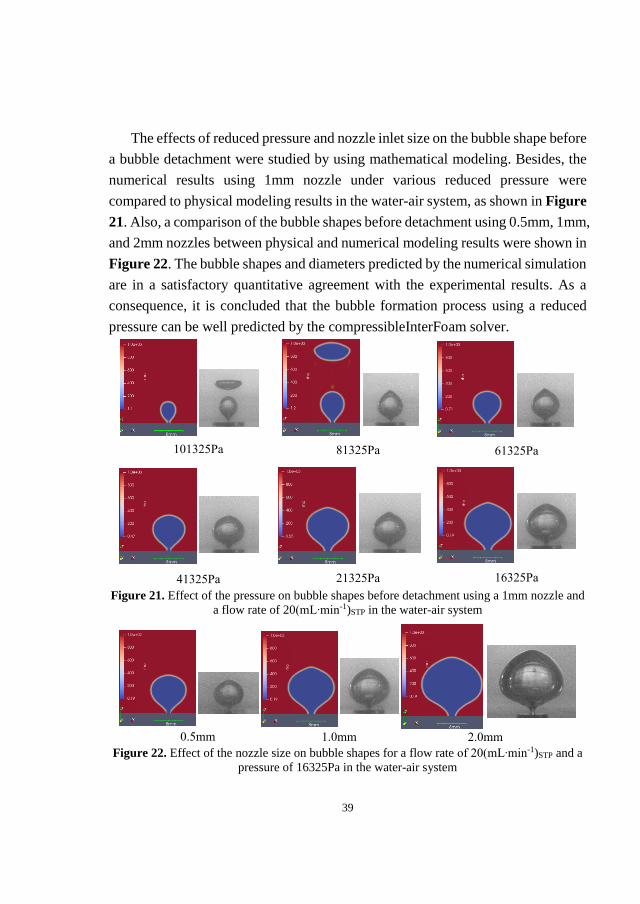
The effects of reduced pressure and nozzle inlet size on the bubble shape before

a bubble detachment were studied by using mathematical modeling. Besides, the

numerical results using 1mm nozzle under various reduced pressure were

compared to physical modeling results in the water-air system, as shown in Figure

21. Also, a comparison of the bubble shapes before detachment using 0.5mm, 1mm,

and 2mm nozzles between physical and numerical modeling results were shown in

Figure 22. The bubble shapes and diameters predicted by the numerical simulation

are in a satisfactory quantitative agreement with the experimental results. As a

consequence, it is concluded that the bubble formation process using a reduced

pressure can be well predicted by the compressibleInterFoam solver.

Figure 21. Effect of the pressure on bubble shapes before detachment using a 1mm nozzle and

a flow rate of 20(mL‧min-1)STP in the water-air system

Figure 22. Effect of the nozzle size on bubble shapes for a flow rate of 20(mL‧min-1)STP and a

pressure of 16325Pa in the water-air system

101325Pa 81325Pa 61325Pa

41325Pa 21325Pa 16325Pa

0.5mm 1.0mm 2.0mm

40

Based on the result of physical modeling studies, it can be seen that the stable

bubble size under a vacuum condition becomes much larger than that for an

atmosphere condition. The reduced pressure has a significant influence on the

initial bubble size. Especially, for high flow rates, the bubble formation is

extremely unstable because the original bubble size is oversized. For a pressure of

16325Pa at the top and a flow rate of 20(mL‧min-1)STP, the bubble rising was shown

in Figure 23. Because of interfacial surface tension, the bubble’s boundary at the

bottom concaves into bubble inside. Thereafter, it deforms into wave shape, so that

the deformed part of bubble is gradually separated from the main body of bubble

at the bottom. After the bubble gradually reaches the stable condition, the deformed

part of bubble bursts into several small bubbles, which rise along with the main

bubble due to the function of wake flow directed by the main bubble. During the

bubble’s rising, the bubble gradually deforms from a spherical shape to a spherical-

cap shape due to the surface tension and the drag force. Finally, the bubble rises

under a quasi-steady shape condition. Using the nozzle’s diameter as an 8mm ruler,

the maximum width of bubble during rising is around 20mm.

Besides, the compressibleInterFoam solver was employed to model the

compressible multiphase flow in the water-air system. Using the same condition

for the physical modeling, the predicted behavior of bubble’s rising was shown in

Figure 24. Under a laminar condition, the maximum bubble width is 20mm when

the bubble becomes steady. This is consistent with the results for a reduced

pressure condition in the physical modeling experiments. Therefore, the

compressibleInterFoam solver is dependent on modeling the bubble’s rising

behavior when assuming a reduced pressure condition.

41

Figure 23. Behavior of Bubble rising under a reduced pressure condition in the water-air system

Figure 24. Mathematical modeling of bubble rising under a reduced pressure in the water-air

system

0.100s 0.090s

0.110s

20mm 20mm

20mm

0s 0.040s

0.080s

20mm 20mm 20mm

0.120s

0.200s

0.160s

20mm 20mm 20mm

0.02s 0.04s

0.08s 0.10s

0.12s 0.14s

0.18s 0.20s

42

Consequently, the compressibleInterFoam solver was used to predict the

motion of bubbles in the refining ladle under a vacuum condition. During the single

bubble’s rising, the bubble deforms from a spherical shape to a spherical-cap shape

because of the surface tension. Therefore, it gradually reaches the stable condition

by means of shedding several small bubbles at the bottom of the main bubble.

When the bubbles become steady, the maximum bubble size is around 65.0mm,

when the surrounding pressure is 0.2bar. In terms of the effect of pressure on the

bubble’s steady condition, the behavior of bubble rising under the high pressure at

the bottom position in the liquid steel was compared to a case corresponding to a

low pressure condition at the top position in the liquid steel. When the pressure

increases, the maximum width of bubble decreases. At the bottom position in the

liquid steel, the steady bubble width is around 58mm, when the surrounding

pressure is 2.0bar.

4.5 Decarburization in an Electric Arc Furnace using Coupled Fluid

dynamics and Thermodynamics (Supplement Ⅵ)

Based on the previous works on the fluid dynamics of gas bubbling, the

coupling method, named the Multi-zone Reaction Model, was employed to

study the thermodynamics reactions between oxygen and molten steel in an

EAF process. At the beginning of the refining period, the carbon mass

percentage is assumed to be 0.00065. For an oxygen flow rate of 100Nm3/h,

during the refining phase, the minimum of carbon mass percent is 0.00005 at

the hot spot zone. After 5min of refining, the carbon mass percent outside the

central plume zone gradually decreases to around 0.00055. Based on the

industrial measurement of the carbon content at the beginning and end points,

the decrease of average carbon content is simplified by assuming a linear

relation with the refining time. Monitoring the average carbon mass percent in

the whole furnace, the decarburization rate is consistent with the ones measured

in the industrial operation, as seen in Figure 25(a). In the industrial operation,

the temperature measurements were carried out to monitor the dynamic

temperatures at the hot spot zone. The maximum and minimum hot spot

43

temperatures are consistent with the measured values in the refining phase, as

shown in Figure 25(b). During the refining, the hot spot temperature gradually

decreases from 2600°C to 2450°C. With a decreasing carbon content in the whole

furnace, the carbon supplement rate from outside to the hot spot zone becomes

slower. Besides, because the reactions of carbon and iron oxidations are

exothermic, the equilibrium reaction rates also drop dramatically. Moreover, in the

range of hot spot temperatures measured in industrial operations, there could exist

an endothermic iron evaporation, which would also results in a temperature

reduction.

(a) (b)

Figure 25. Comparison of industrial measurements and modeling results

(a) average carbon contents and (b) hot spot temperatures

Based on the decarburization process for a flow rate of 100Nm3/h oxygen, the

refining condition with a flow rate of 50Nm3/h oxygen was compared. Moreover,

the combination of oxygen and inert gas argon was used to increase the efficiency

of refining process. In comparison to the gas injection conditions of 50Nm3/h

oxygen, 100Nm3/h oxygen, and a combination of 50Nm3/h oxygen with 50Nm3/h

argon, the average carbon contents, hot spot temperatures and average

temperatures increase with time were shown in Figure 26. For flow rates of

50Nm3/h oxygen and a combination of 50Nm3/h oxygen with 50Nm3/h argon, the

average carbon mass percent gradually decrease to 0.00061 and 0.00058 in the

steel bath, and the average steel temperatures increase to 1773.6K and 1773.9K

1900

2000

2100

2200

2300

2400

2500

2600

2700

0 60 120 180 240 300 360 420 480 540 600 660

Ho

t S

pot

Tem

per

ature

(°C

)

Time (s)

Measured Modeled

0.0004

0.00045

0.0005

0.00055

0.0006

0.00065

0.0007

0.00075

0 60 120 180 240 300

Aver

age

Car

bon

Mas

s F

ract

ion

Time (s)Modeling Trial 1350 Trial 1351Trial 1352 Trial 1354

44

after 5min refining time. The results show that, in comparison to the

decarburization rate under a flow rate of 100Nm3/h oxygen, the decarburization

rate decreases approximately 66% for a flow rate of 50Nm3/h oxygen. Using

the combined injection of 50Nm3/h oxygen with 50Nm3/h argon, the

decarburization rate only drops approximately 38%, due to the efficient kinetic

mass transfer. In comparison to the hot spot temperature under the flow rate of

100Nm3/h oxygen, the temperature for a flow rate of 50Nm3/h oxygen

decreases from a level of 2500°C to a level of 2160°C. That is to say, the hot

temperature decreases to a value of 340°C. For a combined injection of

50Nm3/h oxygen with 50Nm3/h argon, the hot spot temperature is at the level

of 2210°C during the refining. This means that the hot spot temperature

increases almost 50°C in comparison to that for a 50Nm3/h oxygen flow rate.

It is shown that the oxygen flow rate has a large influence on the hot spot

temperature as well as the increase of average steel temperature. Moreover, the

maximum hot spot temperature decreases for the parallel injection conditions

are similar to that for an industrial injection of 100Nm3/h oxygen.

(a) (b)

0.0005

0.00055

0.0006

0.00065

0.0007

0 60 120 180 240 300

Aver

age

Car

bon

Mas

s F

ract

ion

Time (s)

50Nm3/h O2

100Nm3/h O2

50Nm3/h O2+50Nm3/h Ar1773

1773.5

1774

1774.5

1775

0 60 120 180 240 300

Aver

age

Ste

el T

emper

atu

re (

°C)

Time (s)

50Nm3/h O2

100Nm3/h O2

50Nm3/h O2+50Nm3/h Ar

45

(c)

Figure 26. Parameter variation under combined injections of oxygen and inert gas argon

(a) Average carbon content, (b) Average steel temperature, and (c) Hot spot temperature.

For the combined injection of O2 and CO2, the distributions of carbon mass

fraction and temperature in the molten steel with the CO2 mass fractions of 0%,

20%, and 40% after 2.5min refining were compared in Figure 27. With an

increased the ratio of CO2, the mass percent of carbon in the molten steel increases

and the steel temperature decreases. This means that the decarburization rate

gradually decreases for the same refining time. As the carbon dioxide in the gas

injection increases to a 40% mass percentage value, there exists the plume

temperature above the hot spot zone lower than that outside the central plume zone.

1800

2000

2200

2400

2600

2800

0 60 120 180 240 300

Ho

t S

po

t T

emp

erat

ure

(°C

)

Time (s)

50Nm3/h O2

100Nm3/h O2

50Nm3/h O2+50Nm3/h Ar

46

(a) (b)

(c) (d)

(e) (f)

Figure 27. Distribution of carbon mass fraction and temperature in the molten steel for a flow

rate of 100Nm3/h after 2.5min refining phase

(a) and (b) are total O2, (c) and (d) are 20% mass percent of CO2,

(e) and (f) are 40% mass percent of CO2.

47

Chapter 5 Conclusions

This dissertation focuses on the fluid dynamics of gas bubbling and its

advanced coupling with the equilibrium thermodynamics to predict complicated

chemical reactions in the metallurgical processes. Most of the existing works do

not consider the effects of pressure changes and plug designs on the bubble

behavior, and the injection pattern of gas bubbling for a constant bubble size is

usually established by experience, for which the mathematical modeling to

describe the flow field normally has lower accuracy. Based on each multiphase

model’s speciality, numerical simulations have been performed to describe the

bubble behavior using a multi-scale approach: Prototype scale (macro) → Plume

scale → Single bubble scale → Equilibrium reaction scale (micro). The main

content can be divided into two parts:

(1) A solution to the mentioned problems, namely the general empirical rules of

mixing and homogenization, multiphase-model comparison, vacuum bubbling

and statistical bubble interaction, have all been involved in this study.

(2) Based on the analysis of the fluid dynamics of the gas bubbling, a coupled

method of fluid dynamics and thermodynamics, named as Multi-zone

Reaction Model, has been developed to predict the decarburization process in

an EAF with a refining phase.

Several specific conclusions from each supplement can be summarized as

follows:

Review of existing approaches of physical modeling and mathematical

modeling (Supplement Ⅰ)

1.1 Depending on the research purpose, previous physical modeling experiments

in lab scale have been divided based on four major research focuses: ⅰ) mixing

and homogenization in the ladle, ⅱ) gas bubble formation, transformation, and

interactions in the plume zone, ⅲ) inclusion behavior, and ⅳ) steel-slag

48

interface and open eye formation. Several works related to industrial research

focused on open eye formation and the optimization of gas stirring. Concerning

physical modeling, such as mixing and homogenization in ladles, the general

empirical rules can be improved.

1.2 According to the basic fundamental theory and applicability of each model,

four kinds of multiphase-models (Quasi-steady State Model, VOF Model,

Euler-Euler Model, and Euler-Lagrange Model) coupled with three kinds of

turbulence models (k-epsilon Model, k-omega SST Model, LES Model),

particularly paying attention to different research directions have been

discussed. The difference between the four models is in the method how to

describe the liquid-gas two phase zone.

1.3 Based on the literature review, several weaknesses were found: ⅰ) for physical

modeling, such as mixing and homogenization in ladles, the general empirical

rules can be improved; ⅱ) the mathematical models focusing on inclusion

behavior at the steel-slag interface need to be improved; and ⅲ) the phenomena

governing the transfer of elements, vacuum degassing, and the combination of

fluid dynamics and thermodynamics, such as in desulfurization, need to be

developed further.

Flow field and mixing conditions in a 50t ladle (Supplement Ⅱ)

2.1 In a 50t ladle, for a ±5% homogenization degree, the mixing time with dual

plugs using a radial angle of 180° is the shortest. In addition, the mixing time

using a radial angle of 135° decreases the most with an increased flow rate.

The flow pattern and mixing conditions predicted by mathematical modeling

agree well with the result of the physical modeling.

2.2 For a ±1% homogenization degree, the influence of the tracer’s natural

convection on the homogenization pattern cannot be neglected. This is

especially true for ‘soft bubbling’ cases using a low gas flow rate.

2.3 In the 50t ladle, it is recommended that a separation angle of 160° is chosen for

gas stirring when using dual porous plugs, when the optimal radial position is

around 0.65R.

49

Comparison of Euler-Euler and Euler–Lagrange Approaches in the

mathematical modeling (Supplement Ⅲ)

3.1 In the Euler-Euler approach, differences in axial velocities and turbulent

kinetic energies for various bubble sizes mainly appears in the plume zone. In

the Euler-Lagrange approach, different bubble sizes with the same injection

frequency have a small impact on the turbulence dissipation. For both modeling,

the smaller the bubble diameter is, the larger the axial velocity and turbulent

kinetic dissipation become in the central zone.

3.2 For the bubble coalescence and breakup, according to the comparison of two

modeling approaches, the Euler-Lagrange approach is more accurate in

predicting the flow pattern for gas injection with a porous plug in the ladle.

Plug design and statistic bubble behavior in the physical modeling

(Supplement Ⅳ)

4.1 During bottom blowing using a slot plug, with increasing flow rate, the gas-

liquid plume width does not change significantly, and the periodic behavior of

the bubble statistic amount increases gradually. Otherwise, during bottom

blowing using a porous plug, as the flow rate increases, the central plume

becomes wider, and the periodic characteristic of bubble injection is not

obvious.

4.2 As the porosity increases, the volume fraction of gas and the average bubble

size at the central plume zone increases, while the width of the two-phase

plume zone decreases. The results predicted by the mathematical modeling are

consistent with those of the physical modeling.

4.3 Gas injection using a slot plug promotes kinetic reactions close to the open eye

due to the concentrated plume structure and momentum transfer, and gas

injection using a porous plug promotes a good inclusion removal because of

increasing amount of bubbles.

Single bubble behavior under the reduced pressure condition (Supplement Ⅴ)

5.1 The top pressure has a significant influence on the bubble expansion during

formation under vacuum condition compared with that under atmosphere

50

pressure. For the bubble generation, under the same top pressure, as the flow

rate and nozzle size increases, the bubble diameter before attachment and

generation frequency gradually increase.

5.2 Under the same flow rate, with reduced top pressure, the diameter of the

bubbles increases largely and the generation frequency decreases to a small

extent. Under relatively low flow rates, the frequency of the bubble generation

is sensitive to an increased flow rate, and the frequency becomes almost

constant as the flow rate increases to a certain level. In terms of the bubble

rising behavior, the bubble gradually reaches a stable condition by means of

shedding several small bubbles from the main bubble.

5.3 In the steel-argon system, and using flow rates in the range of 5.0(mL‧min-1)STP

to 2000(mL‧min-1)STP, the original bubble diameter is in the range of 6.0mm to

20.0mm. Under laminar conditions, the maximum bubble width is 65mm for a

low pressure of 0.2bar, and at the bottom region the steady bubble width is

around 58mm for a pressure of 2.0bar. As the surrounding pressure increases,

the maximum size of the bubble, under steady conditions, decreases.

Coupled Fluid dynamics and Thermodynamics (Supplement Ⅵ)

6.1 For a high flow rate, the effect of the nozzle size on the hydrodynamic

condition in the reaction zone of the plume area can be neglected.

6.2 The decarburization rate and hot spot temperature predicted by the

mathematical model are consistent with the industrial measurements. The

maximum hot spot temperature gradually decreases during the refining phase.

Also, the oxygen flow rate has a significant influence on the decarburization

rate, hot spot temperature and average steel temperature increment rate.

6.3 In terms of a combined injection of O2 and inert argon gas, while using the

same injected mass of O2, the decarburization rate increases due to the efficient

kinetic mass transfer of carbon in the molten steel. Furthermore, for a combined

injection of O2 and CO2, as the ratio of CO2 mass fraction increases, the

maximum hot spot temperature, the increment rate of average temperature, and

the decarburization rate in the molten steel decrease dramatically. Also, an

51

endothermic reaction of CO2 with carbon in the molten steel occurs, which

results in a temperature drop above the hot spot zone.

Consequently, the research step from fluid dynamics to its coupling with high

temperature, multiphase thermodynamics is a large promotion in this study.

Moreover, the research process using open source software to replace the

commercial software is also believed to be an important technical route to further

facilitate the transparent development of new modules for high temperature

thermodynamics processes such as those in the steel industry.

53

Chapter 6 Sustainability and Recommendations for Future Work

6.1 Sustainability

The iron and steel industry is one of the biggest industrial emitters of CO2,

accounting for between 4% and 7% of anthropogenic CO2 emissions globally.[177,

178] This thesis contributes to a more sustainable and high efficient steelmaking

processes. By implementing the results of optimizing the processes, the production

efficiency can be increased. This leads to energy savings and a decrease of CO2

emissions in the steelmaking processes. In comparison to the traditional ore-based

steelmaking process using a BOF convertor, the scrap-based EAF process itself is

more efficient and environmentally friendly since it leads to a reduction of ore and

fossil resources’ consumption. Furthermore, in the EAF process, the oxygen

injection by bottom-blown is more efficient and results in a lower oxygen

consumption compared to a top-blown oxygen injection. The partial replacement

of argon using the recycled CO2 is developed as an alternative option for the gas

stirring with the aim to decrease the CO2 emissions. In the ladle refining, the

optimal gas stirring condition can increase the process efficiency to reduce the

temperature drop and the resulting need for reheating by using electrodes. Overall,

the implementation of the results in this dissertation contributes to the following

United Nations goals: goal 12 responsible production and goal 13 climate

action.[179]

6.2 Recommendation for Future Work

Further studies on the coupling model to predict the thermodynamic reactions

in the EAF process should be performed. Moreover, the factors to influence fluid

dynamics in the metallurgical processes should be taken into consideration

comprehensively. Several aspects are recommended to study more in-depth:

54

(1) Coupling approach of fluid dynamics and thermodynamics by considering a

combination of CxHy with O2, electrode carbon element addition and electric

arc heating energy source in the EAF furnace.

(2) Specific study on the effect of sharp and dispersed multiphase interface on the

elements transfer in the mathematical modeling

(3) Lab-scale experiments to validate the results from the coupled modeling results

of fluid dynamics and thermodynamics.

(4) Studies of plug designs and configurations on the homogenization degree in the

physical modeling for a reduced top pressure condition.

55

References

1. NSC, 2017, An introduction to steelmaking (https://www.newsteelconstruction.com/wp/an-

introduction-to-steelmaking/).

2. new development and operational results in the use offxied side-wall injectors in the electric arc

furnaces, D. Tolazzi, C. Candusso, and S. Marcuzzi, 2016.

3. D. Mazumdar and R. I. L. Guthrie. ISIJ Int., 1995, vol. 35, pp. 1-20.

4. L. F. Zhang and S. Taniguchi. Int. Mater. Rev., 2000, vol. 45, pp. 59-82.

5. D. Sichen. Steel Res. Int., 2012, vol. 83, pp. 825-41.

6. G. Irons, A. Senguttuvan, and K. Krishnapisharody. ISIJ Int., 2015, vol. 55, pp. 1-6.

7. D. Mazumdar and J. W. Evans. ISIJ Int., 2004, vol. 44, pp. 447-461.

8. Y. Liu, M. Ersson, H. P. Liu, P. G. Jönsson, and Y. Gan. Metall. Mater. Trans. B, 2019, vol. 50,

pp. 555-577.

9. J. Mandal, S. Patil, M. Madan, and D. Mazumdar. Metall. Mater. Trans. B, 2005, vol. 36, pp.

479-87.

10. N. Mazumdar, A. Mahadevan, M. Madan, and D. Mazumdar. ISIJ Int., 2005, vol. 45, pp. 1940-

1942.

11. A. Leonard: Overview of Turbulent and Laminar Diffusion and Mixing, Springer Vienna, Vienna,

2009.

12. M. Ek, L. Wu, P. Valentin, and D. Sichen. Steel Res. Int., 2010, vol. 81, pp. 1056-1063.

13. D. Q. Geng, H. Lei, and J. C. He. Int. J. Miner. Metall. Mater., 2010, vol. 17, pp. 709-714.

14. S. P. Patil, D. Satish, M. Peranandhanathan, and D. Mazumdar. ISIJ Int., 2010, vol. 50, pp. 1117-

1124.

15. H. P. Liu, Z. Y. Qi, and M. G. Xu. Steel Res. Int., 2011, vol. 82, pp. 440-58.

16. A. M. Amaro-Villeda, M. A. Ramirez-Argaez, and A. N. Conejo. ISIJ Int., 2014, vol. 54, pp. 1-

8.

17. W. T. Lou and M. Y. Zhu. ISIJ Int., 2014, vol. 54, pp. 9-18.

18. H. Y. Tang, X. C. Guo, G. H. Wu, and Y. Wang. ISIJ Int., 2016, vol. 56, pp. 2161-2170.

19. R. González‐Bernal, G. Solorio‐Diaz, A. Ramos‐Banderas, E. Torres‐Alonso, C. A. Hernández‐

Bocanegra, and R. Zenit. Steel Res. Int., 2017, vol. 89, pp. 1700281.

20. Z. Q. Liu, L. M. Li, and B. K. Li. ISIJ Int., 2017, vol. 57, pp. 1971-79.

21. K. Bölke, M. Ersson, P.Y. Ni, M. Swartling, and P. G. Jönsson. Steel Res. Int., 2018, vol. 89, pp.

1700555.

22. A. S. Gómez, A. N. Conejo, and R. Zenit. J. Appl. Fluid Mech., 2018, vol. 11, pp. 11-20.

23. Y. Sahai and R. I. L. Guthrie. Metall. Trans. B, 1982, vol. 13, pp. 193-202.

24. Alfonso Humberto Castillejos-Escobar: A study of the fluid-dynamic characteristics of turbulent

gas-liquid bubble plumes, Doctoral thesis of British Columbia University, 1986.

25. A. H. Castillejos and J. K. Brimacombe. Metall. Trans. B, 1987, vol. 18, pp. 659-71.

26. A. H. Castillejos and J. K. Brimacombe. Metall. Trans. B, 1987, vol. 18, pp. 649-58.

27. S. H. Kim and R. J. Fruehan. Metall. Trans. B, 1987, vol. 18, pp. 381-390.

28. S. T. Johansen, D. G. C. Robertson, K. Woje, and T. A. Engh. Metall. Trans. B, 1988, vol. 19,

pp. 745-54.

29. P. E. Anagbo and J. K. Brimacombe. Metall. Trans. B, 1990, vol. 21, pp. 637-48.

30. M. Iguchi, H. Takeuchi, and Z. Morita. ISIJ Int., 1991, vol. 31, pp. 246-53.

56

31. Y. Y. Sheng and G. A. Irons. Int. J. Multiphase Flow, 1991, vol. 17, pp. 585-98.

32. Y. Y. Sheng and G. A. Irons. Metall. Trans. B, 1992, vol. 23, pp. 779-88.

33. Y. K. Xie and F. Oeters. Steel Res. Int., 1992, vol. 63, pp. 93-104.

34. Y. K. Xie, S. Orsten, and F. Oeters. ISIJ Int., 1992, vol. 32, pp. 66-75.

35. Y. Y. Sheng and G. A. Irons. Metall. Trans. B, 1993, vol. 24, pp. 695-705.

36. M. Iguchi, H. Kawabata, K. Nakajima, and Z. Morita. Metall. Mater. Trans. B, 1995, vol. 26, pp.

67-74.

37. K. Sakaguchi and K. Ito. ISIJ Int., 1995, vol. 35, pp. 1348-53.

38. Y. Y. Sheng and G. A. Irons. Metall. Mater. Trans. B, 1995, vol. 26, pp. 625-35.

39. T. Tatsuoka, C. Kamata, and K. Ito. ISIJ Int., 1997, vol. 37, pp. 557-61.

40. Y. Kishimoto, Y. Y. Sheng, G. A. Irons, and J. S. Chang. ISIJ Int., 1999, vol. 39, pp. 113-22.

41. D. Guo and G. A. Irons. Metall. Mater. Trans. B, 2000, vol. 31, pp. 1447-55.

42. Z. J. Han and L. Holappa. Steel Res. Int., 2001, vol. 72, pp. 434-38.

43. S. Taniguchi, S. Kawaguchi, and A. Kikuchi. Appl. Math. Modell., 2002, vol. 26, pp. 249-62.

44. Z. J. Han and L. Holappa. Metall. Mater. Trans. B, 2003, vol. 34, pp. 525-32.

45. Z. J. Han and L. Holappa. ISIJ Int., 2003, vol. 43, pp. 292-97.

46. A. Alexiadis, P. Gardin, and J. F. Domgin. Metall. Mater. Trans. B, 2004, vol. 35, pp. 949-56.

47. D. Mazumdar and R. I. L. Guthrie. Metall. Mater. Trans. B, 2010, vol. 41B, pp. 976-989.

48. K. Wichterle. Steel Res. Int., 2010, vol. 81, pp. 356-61.

49. Y. G. Xu, M. Ersson, and P. G. Jönsson. Metall. Mater. Trans. B, 2015, vol. 46, pp. 2628-38.

50. G. C. Wang, H. C. Zhou, Q. R. Tian, X. G. Ai, and L. F. Zhang. ISIJ Int., 2017, vol. 57, pp. 805-

13.

51. P. Gajjar, T. Haas, K. B. Owusu, M. Eickhoff, P. Kowitwarangkul, and H. Pfeifer. Engineering

Science and Technology, an International Journal, 2018.

52. K. B. Owusu, T. Haas, P. Gajjar, M. Eickhoff, P. Kowitwarangkul, and H. Pfeifer. Steel Res. Int.,

2018, vol. 0, pp. 1800346.

53. Albin Rozario, Nurni N. Viswanathan, and Somnath Basu. Metall. Mater. Trans. B, 2018.

54. L. F. Zhang, S. Taniguchi, and K. Matsumoto. Ironmak. Steelmak., 2002, vol. 29, pp. 326-36.

55. M. Söder, P. G. Jönsson, and L. Jonsson. Steel Res. Int., 2004, vol. 75, pp. 128-38.

56. S. Jansson: A study on molten steel/slag/refractory reactions during ladle steel refining,

Licentiate thesis of KTH Royal Institute of Technology, 2005, 91-7178-090-4 (ISBN).

57. Y. J. Kang, L. Yu, and D. Sichen. Ironmak. Steelmak., 2007, vol. 34, pp. 253-61.

58. M. Thunman, S. Eckert, O. Hennig, J. Bjorkvall, and D. Sichen. Steel Res. Int., 2007, vol. 78, pp.

849-56.

59. J. Savolainen, T. Fabritius, and O. Mattila. ISIJ Int., 2009, vol. 49, pp. 29-36.

60. K. Malmberg, M. Nzotta, A. Karasev, and P. G. Jönsson. Ironmak. Steelmak., 2013, vol. 40, pp.

231-37.

61. H. L. Yang, P. He, and Y. C. Zhai. ISIJ Int., 2014, vol. 54, pp. 578-81.

62. S. F. Yang, W. Liu, and J. S. Li. JOM, 2015, vol. 67, pp. 2993-3001.

63. C. Liu, S. F. Yang, J. S. Li, L. B. Zhu, and X. G. Li. Metall. Mater. Trans. B, 2016, vol. 47, pp.

1882-92.

64. Y.L. Zhou, Z.Y. Deng, and M.Y. Zhu. Int. J. Miner. Metall. Mater., 2017, vol. 24, pp. 627-37.

65. K. Yonezawa and K. Schwerdtfeger. Metall. Mater. Trans. B, 1999, vol. 30, pp. 411-18.

66. Kimitoshi Yonezawa and Klaus Schwerdtfeger. Metall. Mater. Trans. B, 1999, vol. 30, pp. 655-

660.

67. Kimitoshi Yonezawa and Klaus Schwerdtfeger. Metall. Mater. Trans. B, 2000, vol. 31, pp. 461-

468.

68. D. Guo and G. A. Irons. Metall. Mater. Trans. B, 2002, vol. 33, pp. 377-84.

69. Subagyo, G. A. Brooks, and G. A. Irons. ISIJ Int., 2003, vol. 43, pp. 262-63.

57

70. M. Iguchi, K. Miyamoto, S. Yamashita, D. Iguchi, and M. Zeze. ISIJ Int., 2004, vol. 44, pp. 636-

38.

71. K. Yonezawa and K. Schwerdtfeger. ISIJ Int., 2004, vol. 44, pp. 217-19.

72. P. Dayal, K. Beskow, J. Björkvall, and D. Sichen. Ironmak. Steelmak., 2006, vol. 33, pp. 454-64.

73. K. Krishnapisharody and G. A. Irons. Metall. Mater. Trans. B, 2006, vol. 37, pp. 763-72.

74. K. Krishnapisharody and G.A. Irons. Metall. Mater. Trans. B, 2007, vol. 38, pp. 367-375.

75. K. Krishnapisharody and G.A. Irons. Metall. Mater. Trans. B, 2007, vol. 38, pp. 377-388.

76. K. Krishnapisharody and G. A. Irons. ISIJ Int., 2008, vol. 48, pp. 1807-09.

77. P. Valentin, C. Bruch, Y. Kyrylenko, H. Kochner, and C. Dannert. Steel Res. Int., 2009, vol. 80,

pp. 552-58.

78. M. Peranandhanthan and D. Mazumdar. ISIJ Int., 2010, vol. 50, pp. 1622-31.

79. L. Wu, P. Valentin, and D. Sichen. Steel Res. Int., 2010, vol. 81, pp. 508-15.

80. K. Krishnapisharody and G. A. Irons. Metall. Mater. Trans. B, 2015, vol. 46, pp. 191-98.

81. N. Lv, L. Wu, H. Wang, Y. Dong, and C. Su. Int. J. Iron Steel Res., 2017, vol. 24, pp. 243-50.

82. D. Mazumdar, P. Dhandapani, and R. Sarvanakumar. ISIJ Int., 2017, vol. 57, pp. 286-95.

83. L. E. J. Pérez, A. Amaro-Villeda, A. N. Conejo, C. Gonzalez-Rivera, and M. A. Ramírez-Argáez.

Mater. Manuf. Process, 2018, vol. 33, pp. 882-890.

84. Y. Sahai and R. I. L. Guthrie. Metall. Trans. B, 1982, vol. 13, pp. 203-11.

85. Y. Sahai and R. I. L. Guthrie. Metall. Trans. B, 1982, vol. 13, pp. 125-27.

86. D. Mazumdar and R. I. L. Guthrie. Metall. Trans. B, 1985, vol. 16, pp. 83-90.

87. D. Mazumdar. Metall. Trans. B, 1989, vol. 20, pp. 967-69.

88. S. Joo and R. I. L. Guthrie. Metall. Trans. B, 1992, vol. 23, pp. 765-78.

89. D. Mazumdar, R. I. L. Guthrie, and Y. Sahai. Appl. Math. Modell., 1993, vol. 17, pp. 255-62.

90. Y. Y. Sheng and G. A. Irons. Can. Metall. Quart., 1998, vol. 37, pp. 265-73.

91. R. S. Bernard, R. S. Maier, and H. T. Falvey. Appl. Math. Modell., 2000, vol. 24, pp. 215-33.

92. M. B. Goldschmit and A. H. C. Owen. Ironmak. Steelmak., 2001, vol. 28, pp. 337-41.

93. S. Ganguly and S. Chakraborty. ISIJ Int., 2004, vol. 44, pp. 537-46.

94. M. Madan, D. Satish, and D. Mazumdar. ISIJ Int., 2005, vol. 45, pp. 677-85.

95. S. Ganguly and S. Chakraborty. Ironmak. Steelmak., 2008, vol. 35, pp. 524-30.

96. M. Ersson, L. Höglund, A. Tilliander, L. Jonsson, and P. G. Jönsson. ISIJ Int., 2008, vol. 48, pp.

147-53.

97. Y. J. Kwon, J. Zhang, and H. G. Lee. ISIJ Int., 2008, vol. 48, pp. 891-900.

98. B. K. Li, H. B. Yin, C. Q. Zhou, and F. Tsukihashi. ISIJ Int., 2008, vol. 48, pp. 1704-11.

99. P. Sulasalmi, A. Karna, T. Fabritius, and J. Savolainen. ISIJ Int., 2009, vol. 49, pp. 1661-1667.

100. C. A. Llanos, S. Garcia-Hernandez, J. A. Ramos-Banderas, J. D. Barret, and G. Solorio-Diaz.

ISIJ Int., 2010, vol. 50, pp. 396-402.

101. A. Huang, H. Harmuth, M. Doletschek, S. Vollmann, and X. Z. Feng. Steel Res. Int., 2015, vol.

86, pp. 1447-54.

102. T. Kulju, S. Ollila, R. L. Keiski, and E. Muurinen. IFAC-PapersOnLine, 2015, vol. 48, pp. 1-5.

103. P. Sulasalmi, V. Visuri, A. Kärnä, and T. Fabritius. Steel Res. Int., 2015, vol. 86, pp. 212-22.

104. Y. G. Xu, M. Ersson, and P. Jönsson. Steel Res. Int., 2015, vol. 86, pp. 1289-97.

105. A. Senguttuvan: Slag Metal Entrainment in Gas-Stirred Ladles, Doctoral thesis of McMaster

University, 2016.

106. U. Singh, R. Anapagaddi, S. Mangal, K. A. Padmanabhan, and A. K. Singh. Metall. Mater. Trans.

B, 2016, vol. 47, pp. 1804-16.

107. Y. G. Xu, M. Ersson, and P. G. Jönsson. ISIJ Int., 2016, vol. 56, pp. 1982-88.

108. A. Senguttuvan and G. A. Irons. ISIJ Int., 2017, vol. 57, pp. 1962-70.

58

109. K. Ramasetti, V. V. Visuri, P. Sulasalmi, and T. Fabritius: A CFD and Experimental Investigation

of slag eye in Gas Stirred Ladle, Proceeding of the 5th International Conference on Fluid Flow,

Canada, 2018.

110. S. T. Johansen and F. Boysan. Metall. Trans. B, 1988, vol. 19, pp. 755-64.

111. O. J. Ilegbusi and J. Szekely. ISIJ Int., 1990, vol. 30, pp. 731-39.

112. O. J. Ilegbusi, J. Szekely, Manabu Iguchi, Hiroaki Takeuchi, and Zen-ichiro Morita. ISIJ Int.,

1993, vol. 33, pp. 474-78.

113. L. Jonsson and P. Jönsson. ISIJ Int., 1996, vol. 36, pp. 1127-34.

114. P. G. Jönsson, L. Jonsson, and D. Sichen. ISIJ Int., 1997, vol. 37, pp. 484-91.

115. O. J. Ilegbusi, M. Iguchi, K. Nakajima, M. Sano, and M. Sakamoto. Metall. Mater. Trans. B,

1998, vol. 29, pp. 211-22.

116. L. Jonsson, D. Sichen, and P. Jönsson. ISIJ Int., 1998, vol. 38, pp. 260-67.

117. L. F. Zhang. Modelling Simul. Mater. Sci. Eng., 2000, vol. 8, pp. 463-76.

118. J. L. Xia, T. Ahokainen, and L. Holappa. Scand. J. Metall., 2001, vol. 30, pp. 69-76.

119. D. Y. Sheng, M. Soder, P. Jönsson, and L. Jonsson. Scand. J. Metall., 2002, vol. 31, pp. 134-47.

120. M. Söder, P. Jönsson, and J. Alexis. Scand. J. Metall., 2002, vol. 31, pp. 210-20.

121. M. Söder: Growth and removal of inclusions during ladle refining, Doctoral thesis of KTH Royal

Institute of Technology, 2004, 91-7283-886-8.

122. J. Zhang and H. G. Lee. ISIJ int., 2004, vol. 44, pp. 1629-38.

123. C. G. Mendez, N. Nigro, and A. Cardona. J. Mater. Process. Tech., 2005, vol. 160, pp. 296-305.

124. L. T. Wang, Q. Y. Zhang, S. H. Peng, and Z. B. Li. ISIJ Int., 2005, vol. 45, pp. 331-37.

125. L. T. Wang, S. H. Peng, Q. Y. Zhang, and Z. B. Li. Steel Res. Int., 2006, vol. 77, pp. 25-31.

126. M. T. Dhotre, B. L. Smith, and B. Niceno. Chem. Eng. Sci., 2007, vol. 62, pp. 7140-50.

127. F. D. Maldonado-Parra, M. A. Ramirez-Argaez, A. N. Conejo, and C. Gonzalez. ISIJ Int., 2011,

vol. 51, pp. 1110-1118.

128. V. De Felice, I. L. A. Daoud, B. Dussoubs, A. Jardy, and J. P. Bellot. ISIJ Int., 2012, vol. 52, pp.

1273-80.

129. A. Huang, H. Z. Gu, M. J. Zhang, N. Wang, T. Wang, and Y. Zou. Metall. Mater. Trans. B, 2013,

vol. 44B, pp. 744-49.

130. W. T. Lou and M. Y. Zhu. Metall. Mater. Trans. B, 2013, vol. 44B, pp. 762-82.

131. W. T. Lou and M. Y. Zhu. Metall. Mater. Trans. B, 2013, vol. 44B, pp. 1251-63.

132. S. Yu and S. Louhenkilpi. Metall. Mater. Trans. B, 2013, vol. 44B, pp. 459-68.

133. S. Yu, J. Miettinen, and S. Louhenkilpi. Mater. Sci. Forum, 2013, vol. 762, pp. 253-59.

134. J. P. Bellot, V. De Felice, B. Dussoubs, A. Jardy, and S. Hans. Metall. Mater. Trans. B, 2014,

vol. 45B, pp. 13-21.

135. W. T. Lou and M. Y. Zhu. Metall. Mater. Trans. B, 2014, vol. 45B, pp. 1706-22.

136. S. Yu: Numerical Modeling of Dehydrogenation and Denitrogenation in Industrial Vacuum Tank

Degassers, Doctoral thesis of Aalto University, 2014.

137. S. Yu, J. Miettinen, and S. Louhenkilpi. Steel Res. Int., 2014, vol. 85, pp. 1393-402.

138. L. M. Li, Z. Q. Liu, B. K. Li, H. Matsuura, and F. Tsukihashi. ISIJ Int., 2015, vol. 55, pp. 1337-

46.

139. W. T. Lou and M. Y. Zhu. ISIJ Int., 2015, vol. 55, pp. 961-69.

140. S. Yu, J. Miettinen, L. Shao, and S. Louhenkilpi. Steel Res. Int., 2015, vol. 86, pp. 466-77.

141. Numerical Simulation of a Gas-Stirred Ladle, H. Zambrano, A. Bencomo, L. Trujillo, and L. Di

G. Sigalotti, 2015.

142. Modeling of Metal-Slag Mass and Momentum Exchanges in Gas-Stirred Ladles, M. Ramírez-

Argáez and C. González-Rivera, 2017.

143. Q. Cao, L. Nastac, A. Pitts-Baggett, and Q. L. Yu. Metall. Mater. Trans. B, 2018, vol. 49, pp.

988-1002.

59

144. F. Karouni, B. P. Wynne, J. Talamantes-Silva, and S. Phillips. Steel Res. Int., 2018, vol. 89.

145. D. Guo and G. A. Irons. Metall. Mater. Trans. B, 2000, vol. 31, pp. 1457-64.

146. D. C. Guo, L. Gu, and G. A. Irons. Appl. Math. Modell., 2002, vol. 26, pp. 263-80.

147. J. Aoki, L. F. Zhang, and B. G. Thomas: Modeling of Inclusion Removal in Ladle Refining, 3rd

Internat. Congress on Science & Technology of Steelmaking, Warrendale, 2005, pp. 319-32.

148. R. Singh, D. Mazumdar, and A. K. Ray. ISIJ Int., 2008, vol. 48, pp. 1033-35.

149. S. W. P. Cloete, J. J. Eksteen, and S. M. Bradshaw. Progress in Computational Fluid Dynamics,

2009, vol. 9, pp. 345-56.

150. S. W. P. Cloete, J. J. Eksteen, and S. M. Bradshaw: A mathematical modelling study of fluid flow

and mixing in full-scale gas-stirred ladles, 2009, 1468-4349.

151. Y.L. Li, L.F. Zhang, and Y. Ren: Fluid Flow, Alloy Dispersion and Inclusion Motion in Argon-

Stirred Steel Ladles, Proceedings of the Extraction and Processing Division Symposium on

Pyrometallurgy in Honor of David G.C. Robertson, San Diego, 2014, pp. 659-66.

152. L. M. Li, Z. Q. Liu, M. X. Cao, and B. K. Li. JOM, 2015, vol. 67, pp. 1459-67.

153. L. M. Li, B. K. Li, and Z. Q. Liu. ISIJ Int., 2017, vol. 57, pp. 1-10.

154. M. Ek, Q. F. Shu, J. van Boggelen, and D. Sichen. Ironmak. Steelmak., 2013, vol. 39, pp. 77-84.

155. N. Å I. Andersson, A. Tilliander, L. Jonsson, and P. G. Jönsson. Steel Res. Int., 2012, vol. 83, pp.

1039-1052.

156. N. Å I. Andersson, A. Tilliander, L. T. I. Jonsson, and P. G. Jönsson. Ironmak. Steelmak., 2013,

vol. 40, pp. 390-397.

157. N. Å I. Andersson, A. Tilliander, L. T. I. Jonsson, and P. G. Jönsson. Steel Res. Int., 2013, vol.

84, pp. 169-177.

158. N. Å I. Andersson, A. Tilliander, L. T. I. Jonsson, and P. G. Jönsson. Ironmak. Steelmak., 2013,

vol. 40, pp. 551-558.

159. L. Jonsson, D. Sichen, and P. Jönsson. ISIJ Int., 1998, vol. 38, pp. 260-267.

160. M. A. T. Andersson, L. Jonsson, and P. G. Jönsson. ISIJ Int., 2000, vol. 40, pp. 1080-1088.

161. M. Andersson, M. Hallberg, L. Jonsson, and P. Jönsson. Ironmak. Steelmak., 2013, vol. 29, pp.

224-232.

162. Q. Wang, Z. He, G. Q. Li, and B. K. Li. Appl. Therm. Eng., 2016, vol. 103, pp. 419-427.

163. Q. Wang, Z. He, G. Q. Li, B. K. Li, C. Y. Zhu, and P. J Chen. Int. J. Heat Mass Transf., 2017,

vol. 104, pp. 943-951.

164. Q. Wang, Y. Liu, G. Q. Li, Y. M. Gao, Z. He, and B. K. Li. Appl. Therm. Eng., 2018, vol. 129,

pp. 378-388.

165. Al-Harbi M., Atkinson H. V., and Gao S. A.: Simulation of molten steel refining in a gas-stirred

ladle using a coupled CFD and thermodynamic model, Proceedings of the XIth MCWASP

(Modelling of Casting), TMS (The Minerals, Metals & Materials Society), 2010.

166. H. Luo and H. F. Svendsen. AIChE Journal, 1996, vol. 42, pp. 1225-1233.

167. H. Luo: Coalescence, breakup and liquid circulation in bubble column reactors, Doctoral Thesis

of Trondheim University, 1993.

168. P. J. O’Rourke: Collective Drop Effects on Vaporizing Liquid Sprays, Doctoral Thesis of

Princeton University, 1981.

169. ANSYS FLUENT Theory Guide Version R3, ANSYS, 2019.

170. ANSYS FLUENT User Guide Version R3, ANSYS, 2019.

171. User Guide version 7, OpenFOAM, 2019.

172. K. Krishnapisharody and G. A. Irons. Metall. Mater. Trans. B, 2013, vol. 44, pp. 1486-98.

173. C. M. Fan and W. S. Hwang. Ironmak. Steelmak., 2002, vol. 29, pp. 415-26.

174. Ultrasound velocity profiler UVP-DUO user’s guide, Released 5.2, 2014.

175. T. Kordel, B. Kleimt, R. Pierre, G. Weides, G. Thomassen, S. Barella, C. Mapelli, L. Bianco, and

A. Viotto, EUR 28970-Determining process conditions for online monitoring of temperature and

60

carbon content in the electric arc furnace to optimize end point control-MELTCON, European

Commission 2018, 9.

176. T. Stapurewicz and N. J. Themelis. Can. Metall. Q., 1987, vol. 26, pp. 123-28.

177. Energy Efficiency and CO2 Reduction in the Iron and Steel Industry, European Commission,

2017.

178. Steel's Contribution to A Low Carbon Future and Climate Resilient Societies, World Steel

Association.

179. United Nations, 2020, Sustainable development: UN’s 17 sustainable development goals

(https://www.un.org/sustainabledevelopment/).