arX

iv:1

008.

3376

v1 [

gr-q

c] 1

9 A

ug 2

010

Thin-shell wormholes in d-dimensional general relativity:

Solutions, properties, and stability

Gonçalo A. S. Dias∗

Centro de Física do Porto - CFPDepartamento de Física e Astronomia

Faculdade de Ciências da Universidade do Porto - FCUPRua do Campo Alegre, 4169-007 Porto, Portugal,

José P. S. Lemos†

Centro Multidisciplinar de Astrofísica - CENTRADepartamento de Física,

Instituto Superior Técnico - IST,Universidade Técnica de Lisboa - UTL,

Av. Rovisco Pais 1, 1049-001 Lisboa, Portugal&

Institute of Theoretical Physics - ITP,Freie Universität Berlin,

Arnimallee 14 D-14195 Berlin, Germany.

We construct thin-shell electrically charged wormholes in d-dimensional general relativity with acosmological constant. The wormholes constructed can have different throat geometries, namely,spherical, planar and hyperbolic. Unlike the spherical geometry, the planar and hyperbolic geome-tries allow for different topologies and in addition can be interpreted as higher-dimensional domainwalls or branes connecting two universes. In the construction we use the cut-and-paste procedureby joining together two identical vacuum spacetime solutions. Properties such as the null energycondition and geodesics are studied. A linear stability analysis around the static solutions is carriedout. A general result for stability is obtained from which previous results are recovered.

PACS numbers: 04.20.Gz, 04.20.Jb, 04.40.-b

I. INTRODUCTION

A. Visser’s book

In physics, in many situations, the study of a system passes through three stages. First, one finds a solutionthat emulates the system itself. Second, in turn, through the solution one studies the peculiarities that the systemmight have. Third, one performs a stability analysis on the solution to gather whether the system can be realistic ornot. Traversable wormhole physics is not different. Throughout its development, traversable wormhole physics hascomplied to this bookkeeping.

The field of traversable wormhole physics has been systematized by Visser in his book “Lorentzian wormholes: fromEinstein to Hawking” [1]. The three stages of wormhole study are in one form or another in the book. For instance,not only it displays several solutions as it also shows how simple wormhole construction can be in the paper. Inaddition, the book emphasizes that one of the most important properties of traversable wormhole physics is that,within general relativity, its constitutive matter must possess one kind or another of exotic properties. Indeed, asthe wormhole geometry, with a throat and two mouths, acts as tunnels from one region of spacetime to another,its constitutive matter possesses the peculiar property that its stress-energy tensor violates at least the null energycondition, i.e., its matter must be exotic. In general, the known classical fields obey the null energy condition butquantum fields in very special circumstances may not obey it. Since the circumstances in which the null energycondition is not obeyed are very restricted, the creation of these exotic fields for wormhole building is a difficulttask. In this setting it is thus important to minimize the usage of exotic fields by finding conditions on the wormholegeometries which can contain arbitrarily small quantities of matter violating the averaged null energy condition. Thishas been clearly explained in Visser’s book [1] and pursued further later [2]. Finally, stability analysis, perhaps themost difficult stage of all, is also studied, though timidly, in the book [1].

∗ Email: goncalo.apra@gmail.com† Email: joselemos@ist.utl.pt

2

B. Wormhole solutions divided into three classes

The wormhole solutions that appeared previously have been put into a wider context through the book [1], which inturn helped to inspire developing the field still further as can be seen by the great many number of solutions dealingwith wormhole physics and geometry that have appeared since. A methodical way of organizing now this field is bydividing wormhole solutions into three classes: I. Wormholes generated by continuous fundamental fields with exoticproperties; II. Wormholes generated from matching an interior exotic solution to an exterior vacuum, at a junctionsurface, (just like one does with relativistic stars); and III. Wormholes generated from exotic thin shells. Class I couldbe thought of as nature given, of cosmological origin. Classes II and III, instead, should be built by cosmic engineers,first by providing the exotic matter, then building the wormhole itself and lastly joining it smoothly into the cosmicvacuum. Class III is the most simple to construct theoretically, and perhaps also practically.

In relation to class I (wormholes from continuous fundamental fields) it is striking that the first wormhole solutionsare indeed of this class [3]. Ellis [3] discussed a wormhole solution, which he called a drainhole, as a model for a particlein general relativity in which an exotic continuous scalar field through spacetime provides the means to open up thethroat and mouths of the wormhole. Bronnikov [3] found a general class of solutions within scalar-tensor theories,among which he managed to glimpse solutions with a neck, as he called it, i.e., wormhole solutions. In the samevein, Kodama [3] studied a wormhole solution, which he called a kink, with an exotic continuous scalar field beingthe necessary field to maintain an Einstein-Rosen bridge open. Many other wormholes, whose subsistence hinges onsome or another form of exotic matter put into the model or on the introduction of interactions of a new type whichin turn mimic the exotic matter itself, have been discussed with profusion. One can name a few of those solutions:wormholes in a cosmological constant scenario, wormhole solutions in semiclassical gravity, wormhole solutions inBrans-Dicke theory, wormholes on the brane, wormholes supported by matter with an exotic equation of state such asphantom energy and tachyon matter, wormholes in nonlinear electrodynamics, wormholes in nonminimal Einstein–Yang-Mills matter originating a Wu-Yang magnetic wormhole, wormholes with nonminimal and ghostlike scalar fieldand nonminimal matter [4]. In this setting, cylindrical wormholes, which permit two definitions of the throat (one ofthem allowing non-violation of the energy conditions), with several classes of fields such as scalar, spinor, Maxwell,and nonlinear electric fields have also been studied [4]. Stability is always a hard issue and only some of these systemshave had their stability analyzed, see [5] as well as some of the works in [4] where for instance the stability of the Elliswormhole is studied.

In relation to class II (wormholes generated from matching an interior exotic solution to an exterior vacuum ata junction surface) there are many interesting works. Morris and Thorne [6] created the idea that an arbitrarilyadvanced civilization could construct wormholes and traverse them to and fro, initiating thus the systematic study oftraversable wormholes, later organized in a coherent whole in [1]. In Morris and Thorne’s work [6] a finite quantityof exotic matter was used in wormhole building. This matter was then to be carefully matched to the environment.In theory this matching is done through the junction conditions. In practice, it certainly can be tricky. Morris -Thorne type of wormholes were later generalized to include a positive or negative cosmological constant in [7], wherea review of wormhole solutions was also taken, and it was suggested that perhaps one should call a civilizationthat constructs wormholes an absurdly advanced civilization rather than an arbitrarily advanced civilization. Otherwormhole solutions generated from matching an interior exotic solution to a vacuum, as well as their exotic matterproperties, have been studied. Namely, other wormholes in spacetimes with a cosmological constant, wormholes on thebrane, wormholes made of phantom energy, wormholes with a generalized Chaplygin gas, Van der Waals quintessencewormholes [8]. For some study of stability of wormholes within this class see [9].

In relation to class III (wormholes generated from exotic thin shells) many solutions have also been studied. Sincethin shells need less matter, the construction of wormholes from thin shells gives an elegant way of minimizing theusage of exotic matter. The exotic matter is concentrated at a shell at the wormhole throat alone, yielding a thinshell wormhole solution. In this limiting case of a thin shell, the throat and the two mouths are all at the samelocation, they are indistinguishable. This concentration of the entire content of exotic matter at the shell throatof the wormhole is provided by the cut-and-paste technique used for the first time in relation to wormholes in [10](see also [1]), although Morris and Thorne [6] had used before heuristic methods in such a construction. Thin-shellwormholes in a cosmological constant background, wormhole with surface stresses on a thin shell, plane symmetric thinshell wormholes with a negative cosmological constant, cylindrical thin-shell wormholes, charged thin-shell Lorentzianwormholes in a dilaton-gravity theory, five dimensional thin-shell wormholes in Einstein-Maxwell theory with a Gauss-Bonnet term, solutions in higher dimensional Einstein-Maxwell theory, thin-shell wormholes associated with globalcosmic strings, wormhole solutions in heterotic string theory, a new type of thin-shell wormhole by matching two tidalcharged black hole solutions localized on a three brane in the five dimensional Randall-Sundrum gravity scenario,thin shell and other wormholes within pure Gauss-Bonnet gravity which can be built without the need of usingexotic matter (the gravity itself being already exotic), spherically symmetric thin-shell wormholes in a string cloudbackground spacetime, and many other solutions have been discussed in detail [11]. Now, in relation to stability,

3

these thin-shell wormholes are extremely useful as one may consider a linearized stability analysis around the staticsolution. In the end, the stability analysis will tell whether the throat can be kept open or not, i.e., whether the staticsolution holds under small perturbations. Within general relativity this has been done for several thin-shell wormholesystems, namely, four-dimensional spherical symmetric systems in vacuum [12], with a cosmological constant [13], andwith electric charge [14], planar systems with a cosmological constant [15], and d-dimensional spherical symmetricsystems with electric charge [16]. Also for stability analyses with dilaton, axion, phantom and other types of matter,and in cylindrical symmetry see [17]. This method does not require a specific equation of state, although it can beadded to the analysis as was done in some works previously cited. One can also apply other techniques like a dynamicstability analysis to these thin-shell wormholes [18].

C. Aim and motivation for this work

In this work we want to extend further the study of class III wormholes, wormholes generated from exotic thin shells.We study here d-dimensional thin shell electrically charged wormhole spacetimes with spherical, planar, and hyperbolicgeometry (each with possible different topologies), with a cosmological constant term within general relativity. Themotivation for this general analysis comes from several fronts.

The study of objects in d-dimensions was already of interest when one invoked Kaluza-Klein small extra dimensionswithin fundamental theories, and it has become even more interesting and important since the proposal of the possibleexistence of a universe with extra large dimensions [19]. Assuming such a scenario of large extra dimensions is correct,one can possibly make tiny small distinct objects such as black holes and wormholes of sizes of the order of the newPlanck scale.

The introduction of a cosmological constant in the study of new objects is advisable since from astronomicalobservations, it seems that we presently live in a world with a positive cosmological constant, Λ > 0, i.e., in anasymptotically de Sitter universe. In addition, a spacetime with Λ < 0, an anti-de Sitter spacetime, is also of significantrelevance since it allows a consistent physical interpretation when one enlarges general relativity into a gauge extendedsupergravity theory in which the vacuum state has negative energy density, i.e., a negative cosmological constant. Ifthese theories are correct, they imply that the anti-de Sitter spacetime should be considered as a symmetric phaseof the theory, although it must have been broken as we do not presently live in a universe with Λ < 0. Moreover aΛ < 0 anti-de Sitter spacetime permits a consistent theory of strings in any dimension, and it has been conjecturedthat these spacetimes have a direct correspondence with certain conformal field theories on the boundary of thatspace, the AdS-CFT conjecture. Even with its preference to negative cosmological constant scenarios, string theorycan, although in a contrived way, produce a landscape of positive cosmological constant universes, indicating perhapsthat one can transit between both signs of the cosmological constant, see [20] for all these aspects related to thecosmological constant.

Once one starts to discuss extra dimensions and a cosmological constant term then the objects under study, blackholes or wormholes, say, can have different geometries and topologies. Indeed, in the Λ < 0 case, besides sphericalsymmetric horizons, black holes can have planar and hyperbolic symmetric horizons, each one of these new geometriesadmitting different topologies [21]. Also, contrary to black holes with a spherical horizon, black holes with planarand hyperbolic symmetric horizons have the property that infinity carries the same topology as the throat. Onecan go beyond black hole solutions and build, upon addition of exotic matter, traversable wormholes with the samecorresponding symmetries and topologies, by natural extension of the corresponding black hole solutions. In these newplanar and hyperbolic geometries, infinity carries the same topology as the throat, whereas in the spherical geometryinfinity is the usual corresponding asymptotic spacetime. In this sense, the construction of the planar and hyperbolicsymmetric wormholes does not alter the topology of the background spacetime (i.e., spacetime is not multiply-connected), so that these solutions can be considered higher-dimensional domain walls or branes. Note that the Λ = 0and Λ < 0 wormhole spacetimes allow valid definitions for the mass and charge, and when the wormholes have rotationangular momentum is also well defined [21]. So, this gives further reasons to study, besides wormhole structures inpositive cosmological constant spacetimes, wormhole structures in zero and negative cosmological constant spacetimes.

Finally, electric charge is a fundamental property of matter, and the electromagnetic field is a fundamental interac-tion between electrically charged objects. Objects with a distribution of electric charge of the same sign suffer internalrepulsion, which counteracts the effects of attractive gravitation. Moreover, the concept of wormholes was invented byWheeler to provide a mechanism for having charge without charge, since the field lines seen in one part of the universecould thread the handles of a multiply connected spacetime and reappear in the other part. This idea was indeedcorroborated by Wheeler and other authors when they showed the Schwarzschild and Reissner-Nordström solutions,when fully extended, really should be interpreted as wormholes, although non-traversable, the latter a wormhole withelectric charge [22]. As such it is always of interest to see the effects of a net electric charge in wormholes.

So these are the fields and matter which we consider in our wormhole and domain wall building. Using the usual

4

cut-and-paste technique [1] we find, from the vacuum solutions, thin-shell electrically charged wormholes with differentgeometric-topologies in d-dimensional general relativity with a cosmological constant. We study the properties of thesolutions and analyze perturbations in the linear regime. Our general solutions encompass previous solutions whichcan be reobtained as particular cases of our analysis. Indeed, previous results in d = 4 and in other dimensions canbe taken from our general expression, in particular the results in [12–16] are reobtained as particular cases.

D. Structure of the work

The paper is structured as follows. In Sec. II we use the cut-and-paste technique in order to build static wormholesfrom the gluing, above the gravitational radius (or the would-be horizon), of the d-dimensional electrically chargedspacetimes, with a negative cosmological constant and with several geometries and topologies. In Sec. III we studythe properties of these wormholes by providing the exotic conditions and analyzing the motion of test particles in thewormhole background. In Sec. IV a linearized stability analysis is performed around the static configurations. Ourgeneral result is then shown to recover previously calculated conditions for static wormholes in particular dimensions,in particular geometries and topologies, with and without electric charge, and with and without a cosmologicalconstant. In Sec. V we conclude. The velocity of light and Newton’s constant are put equal to one throughout.

II. SPACETIME SURGERY AND STATIC WORMHOLES

A. Cut-and-paste techniques

We consider Einstein’s equations in the form

Gαβ +(d− 1)(d− 2)

6Λ gαβ = 8 π Tαβ , (1)

where Gαβ is the Einstein tensor, d is the dimension of the spacetime, Λ is the cosmological constant, gαβ is thegeneric metric, and Tαβ is the energy-momentum tensor. Greek indices are spacetime indices, latin indices arespacetime indices out of the shell. Equation (1) is supplemented by the Maxwell equation, but since it is rathertrivial, it is not necessary to explicitly display it.

The general static metric solution for a d-dimensional vacuum spacetime, with electric charge, cosmological constantand different (d− 2) geometric-topologies is given in the form

ds2 = −f(r)dt2 + f(r)−1dr2 + r2dΩkd−2 , (2)

with the metric function f(r) given by

f(r) = k − Λ r2

3− M

rd−3+

Q2

r2(d−3), (3)

and where t, r, θ1, . . . , θd−2 are Schwarzschildean coordinates, M and Q are mass and charge parameters, respectively,and the cosmological constant Λ being zero or of either sign, Λ < 0, Λ = 0, and Λ > 0. Here k is the geometric-topological factor of the (d − 2)-dimensional t = constant, r = constant surfaces, with k = 1, 0,−1 for spherical,planar, and hyperbolic geometries, respectively. The spherical geometry can only have (d − 2)-dimensional surfaceswith spherical topology and with infinity behaving normally. On the other hand, the (d− 2)-dimensional hyperbolicand planar geometries can have different topologies, depending on whether they are infinite in extent or somehowcompactified to produce different (d − 2)-dimensional surfaces, and with infinity following the topology of those(d − 2)-dimensional surfaces. For instance, in d = 4 the situation simplifies, the t = constant, r = constant surfacesare 2-surfaces and can be classified. For spherical symmetry each 2-surface is compact (genus zero) spherical surface.In planar geometry each 2-surface can be an infinite plane, a cylindrical surface, or a compact (genus one) toroidalsurface. In hyperbolic geometry each 2-surface can be an infinite hyperbolic plane, or a compact (genus two orgreater) toroidal surface with several holes. For surfaces in higher dimensions the topologies can be even a lot morecomplicated [21]. Now, (dΩk

d−2)2 is given by three different expressions according to the value of the parameter k,

dΩ1d−2 = dθ21 + sin θ21 dθ

22 + . . .+

d−3∏

i=2

sin θ2i dθ2d−2 ,

5

dΩ0d−2 = dθ21 + dθ22 + . . .+ dθ2d−2 ,

dΩ−1d−2 = dθ21 + (sinh θ1)

2 dθ22 + . . .+ (sinh θ1)2d−3∏

i=2

sin θ2i dθ2d−2 . (4)

One should note that the mass and charge terms above in Eq. (3), that is M and Q, are not the ADM mass andcharge of the solutions, but rather M and Q are parameters proportional to the ADM mass and electric charge,

respectively. For instance, in the spherical case and for zero cosmological constant one has m =(

(d−2)Σ 1d−2

8π

)

M , and

q2 =(

(d−2) (d−3)2

)

Q2, where m and q are the ADM mass and electric charge, respectively, and Σ 1d−2 is the area of the

(d− 2)-dimensional unit sphere, Σ 1d−2 = 2π

d−12 /Γ

(

d−12

)

. When Λ > 0 the ADM quantities are not well defined. Thezeros of f(r) in Eq. (3) give the gravitational radius rg. The full metric vacuum solution given in Eqs. (2)-(3), whenextended to all r (0 ≤ r < ∞), yield black hole solutions. Thus, in studying wormholes the matter is put outside thegravitational radius rg.

We now consider two copies of the vacuum solution, Eqs. (2)-(4), removing from each copy the spacetime regiongiven by

Ω± ≡ r± ≤ a | a > rg , (5)

where a is a constant and rg is the gravitational radius given as the largest positive solution r = rg to the equationf(r) = 0. The latter condition, a > rg, is important in order not to have an event horizon. With the removal ofthese regions of each spacetime, we are left with two geodesically incomplete manifolds, with the following timelikehypersurfaces as boundaries

∂Ω± ≡ r± = a | a > rg . (6)

The identification of these two timelike hypersurfaces, ∂Ω+ = ∂Ω− ≡ ∂Ω, results in a manifold, now geodesicallycomplete, where two regions are connected by a wormhole. This wormhole has a throat at ∂Ω, which is the separatingsurface between the two regions Ω±. In fact, this cut-and-paste technique treats the throat as a hypersurface betweentwo regions of spacetime, where all the exotic matter is concentrated, making the wormhole solution a thin-shellwormhole solution. In this thin-shell case the location of the two mouths coincide with that of the throat. To continuethe analysis we need to use the Darmois-Israel formalism. The intrinsic metric of this separating hypersurface ∂Ω cannow be written as

ds2∂Ω = −dτ2 + a2(τ)(dΩkd−2)

2 , (7)

with τ being the proper time along the hypersurface ∂Ω, and a(τ), a quantity that defines the radius at which thethroat is located in each partial manifold Ω±, now a function of the proper time of the throat. In the bulk spacetime,the coordinates of this hypersurface are given by xα(τ, θ1, θ2, . . . , θd−2), with the respective 4-velocity written as

uα± ≡ dxα

dτ. (8)

The intrinsic stress-energy tensor is defined through the Lanczos equation as

Sij = − 1

8π(κi

j − δijκll) , (9)

where the indices written in the latin alphabet run as i = (τ, θ1, . . . , θd−2). The quantity κij represent the discontinuityin the extrinsic curvature Kij , and one has κij = K+

ij −K−ij . Each of the extrinsic curvatures, on each of the original

manifolds Ω±, is defined through

K±ij =

∂xα

∂ξi∂xβ

∂ξj∇±

αnβ

= −nγ

(

∂2xγ

∂ξi∂ξj+ Γγ ±

αβ

∂xα

∂ξi∂xβ

∂ξj

)

, (10)

where nα is the unit normal to ∂Ω in the bulk spacetime, the ± superscripts refer to the spacetime parcel Ω±, andΓγ ±αβ refers to the respective spacetime Christoffell symbols. The parametric equation for the hypersurface ∂Ω can be

written as f(xα(ξi)) = 0. Using this equation we arrive at the formula for the normal vector

nα = ±∣

∣

∣

∣

gαβ∂f

∂xα

∂f

∂xβ

∣

∣

∣

∣

− 12 ∂f

∂xα. (11)

6

It can be ascertained that nαnα = +1, which makes it spacelike, indeed nα is normal vector to a timelike hypersurface.Applying Eqs. (8) and (11) to our case, we have xα(τ, θ1, . . . , θd−2) = (t(τ), a(τ), θ1, . . . , θd−2), with the 4-velocitywritten as

uα± =

(

√

f(r) + a2

f(r), a, 0, . . . , 0

)

, (12)

and the normal vector nα± as

nα± =

(

−a,

√

f(r) + a2

f(r), 0, . . . , 0

)

, (13)

where ˙≡ ∂ /∂τ . This last result can be arrived at through the relations uαnα = 0 and nαnα = +1, as well as throughthe relation (11). Given the symmetry properties of the solutions we are working with, the discontinuity of the extrinsic

curvatures can be written as κij = diag(κτ

τ , κθ1θ1, . . . , κ

θd−2

θd−2). This allows us to write the surface intrinsic energy-

momentum tensor as Sij = diag(−σ, P , . . . , P), where σ is the surface energy density and P is the surface pressure.

From the Lanczos equation, Eq. (9), we obtain S00 = − 1

8π

(

κ00 − κl

l

)

= 18π (κ

11 + κ2

2 + . . .+ κd−2d−2) =

(d−2)4π a

√

f + a2, andso,

σ = − (d− 2)

4π a

√

f + a2 . (14)

Using S11 we obtain

P =1

8π

2a+ f ′√

f + a2− d− 3

d− 2σ . (15)

For the latter results we have used the following expressions for the extrinsic curvatures, defined in Eq. (10), K0±0 =

±12 f

′+a√f+a2

, K1±1 = ± 1

a

√

f + a2, K2±2 = ± 1

a

√

f + a2, and so on. One can substitute one of the two equations (14) and

(15) by the conservation equation, which can be written as

d

dτ(σ ad−2) + P d

dτ(ad−2) = 0 . (16)

In order to solve Eqs. (14)-(15), or if we prefer Eqs. (14) and (16), for σ(τ) and a(τ), one would need to choose anequation of state, the most simple one would be a cold equation of state P = P(σ).

B. Static wormholes

Now, we resort to a static shell for which a = a = 0. In this case Eqs. (14) and (15) reduce to

σ = − (d− 2)

4π a

√

f , (17)

P =a f ′ + 2(d− 3) f

8π a√f

, (18)

A general equation of state of the form P = P(σ) turns the terms in f(a), such as M , Q, a, and Λ into related terms,that is, there is a relation between these terms, making them dependent upon each other.

III. WORMHOLE PROPERTIES: ENERGY CONDITIONS AND TEST PARTICLE MOTION

A. Wormhole and domain walls

These traversable wormhole solutions are a natural extension of the corresponding black hole solutions upon theaddition of exotic matter. For the plane and hyperbolic traversable wormhole solutions, infinity carries the sametopology as the the topology of the t = constant, r = constant (d − 2)-dimensional surfaces of the backgroundspacetime. Thus, the construction of these wormholes does not alter the topology of the background spacetime (i.e.,spacetime is not multiply-connected). Therefore, these solutions can instead be considered higher-dimensional domainwalls or branes connecting two universes, and as such, in general, do not allow time travel.

7

B. Energy conditions

1. The throat shell

Now we turn to the issue of the energy conditions on the shell. In our case the weak energy condition is givenby σ + P ≥ 0 and σ ≥ 0. Since, in the reference frame we are working, the surface energy density is negative, seeEq. (17), this means that the weak energy condition is violated as usual for wormholes. The null energy conditionrequires only that σ + P ≥ 0. Using (17)-(18) this implies the following inequality

ad−3(

2 ad−3k − (d− 1)M)

+ 2(d− 2)Q2 ≥ 0 . (19)

We can further require that the strong energy condition holds, i.e., σ + (d− 2)P ≥ 0, which using (17)-(18) yields

(d− 4)k − (d− 3)

3Λ a2 − (d− 5)M

2 ad−3− Q2

a2(d−3)≥ 0 . (20)

2. The two exterior regions to the shell

Now we turn to the issue of the energy conditions outside the shell, i.e., for r > a. Here only the electromagneticfield and Λ contribute to the energy-momentum tensor of the Einstein equations, see [16] for the case of sphericalsymmetry (k = 1). The energy-momentum tensor of the electromagnetic field is T em

αβ = 14π

(

−F γαFβγ − 1

4gαβFγδFγδ)

.

The only nonzero component of the electromagnetic field is Er = Qrd−2 . Calculating the T em

00 component of the energy-

momentum tensor yields T em00 = 1

8π f(r) Q2

r2(d−2) . We can write the T em11 component as T em

11 = − 18π f(r)−1 Q2

r2(d−2) . Wehave also to include the vacuum energy represented by the cosmological constant. The corresponding vacuum energy-momentum tensor can be written as T vac

αβ = − Λ8π gαβ . Thus, T vac

00 = Λ8πf(r), T

vac11 = − Λ

8πf−1(r) , T vac

22 = − Λ8π r

2, and

so on. Using uα = (−√f, 0, . . . , 0) for a timelike, future directed vector field, and T00 = ρf(r) , T11 = prf(r)

−1,

T22 = pθ1r2, T k=1

33 = pθ2r2 sin θ21, T k=0

33 = pθ2r2, T k=−1

33 = pθ2r2 sinh θ21 , we can establish that the weak energy

condition, Tµνuµuν ≥ 0, is satisfied if

Q2 ≥ −Λ r2(d−2) , (21)

implying that if Λ < 0, then the weak energy condition is satisfied only if∣

∣Q2∣

∣ ≥√

|Λ| rd−2, and if Λ < 0, then the

weak energy condition is always satisfied, because Q2 > 0 and Λ > 0 make it always true. There is no dependence onthe topological factor k. So, outside the shell, where the contributions to the energy-momentum tensor come from theelectromagnetic field and the cosmological constant, the weak energy condition is not satisfied except in a finite region,if |Q| is large enough, in the case of anti-de Sitter spacetimes. As to the null energy condition, it always holds. Thiscan be gleaned from the fact that Tµνk

µkν = 0, where the kµ are null vectors, defined as kµ = (− 1√f,√f, 0, . . . , 0),

where f is again the metric function, and the Tµν is the same as above, the sum of the electromagnetic and vacuumenergy-momentum tensors.

C. Attraction and repulsion of the wormhole on test particles

In order to complete the general considerations on the properties of the static wormholes of the family of solutionsunder study, we address the issue of the attractive or repulsive character of the traversable wormhole on test particles.First, let us recall the 4-velocity in Eq. (12) now for a test particle. The expression contains the term a2 inside thesquare root. For the static wormhole case under consideration it holds that a2 = 0. So the 4-velocity is now writtenas

uα± =

(

1√

f(r), 0, . . . , 0

)

(22)

The 4-acceleration is aα = uα;β u

β. Now, given the expression for uα in Eq. (22) we have

aα = uα;0 u

0 = uα;0

1√

f(r). (23)

8

We can show that uα;0 = uα

,0+Γαα0 u

α = Γα00u

0. The only nonzero component of this is α = 1, such that u1;0 = Γ1

00u0.

From this we know that aα = (0, ar, 0, . . . , 0), where ar = 12f

′(r). Expanding, we get

ar = −Λ

3r +

(d− 3)M

2 rd−2− (d− 3)Q2

r2d−5. (24)

The geodesic equation, d2rdτ2 + Γ1

00x0x0 = 0, allows us to write

d2r

dτ2= −Γ1

00

(

d2t

dτ2

)

= −ar . (25)

As in [15] an observer must maintain a proper acceleration with the radial component given in Eq. (24) in order toremain at rest. Again, the wormhole is attractive if ar > 0 and repulsive if ar < 0, which depends on the balancingof the parameters in Eq. (24).

IV. STABILITY ANALYSIS: LINEAR STABILTY

A. General considerations: the stability equations and criteria

The equations of motion (14) and (16) can be put in the more useful form

a2 −

−Λ

3a2 − M

ad−3+

Q2

a2(d−3)− 16 π2 a2

(d− 2)2σ2(a)

= −k , (26)

and

σ = −(d− 2)a

a(σ + P) , (27)

respectively. One can choose a particular equation of state, for instance, an equation of state taken from the genericcold equation of state P = P(σ). Then we can integrate Eq. (27) to yield the general solution ln a = − 1

d−2

∫

dσσ+P(σ) ,

which, if we wish, can be formally inverted to provide the function σ = σ(a), i.e., the wormhole surface density as afunction of its own radius. Substituting this equation for ln a into Eq. (26) determines the the motion of the throat,and so its stability.

We follow other path provided by Poisson and Visser [12]. In order to test stability we consider a linear perturbationaround those static solutions found in Sec. II B. Let us take a0 as the radius of the static solution. The respectivestatic values of the surface energy density and the surface pressure are given by Eqs. (17)-(18). To know whether theequilibrium solution is stable or not, one must analyze the shell’s equation of motion near the equilibrium solution.Following [12] we put quite generally

P = P(σ) , (28)

i.e., we impose a generic, as opposed to a particular, cold equation of state. Now, Eq. (26) can be written in the moreuseful form

a2 = −V (a) , (29)

with V (a) given by

V (a) = k − Λ

3a2 − M

ad−3+

Q2

a2(d−3)− 16 π2 a2

(d− 2)2σ(a)2 , (30)

or more compactly as,

V (a) = f(a)− 16 π2 a2

(d− 2)2σ(a)2 . (31)

In the study of the stability of a static solution of radius a0, of course we are considering f(a0) in the interval f(a0) > 0so that no event horizon is present. Our initial condition before the cutting and gluing operation is that a > rg, hence

9

a0 > rg. A linearization is going to be done in order to determine whether and in what conditions the static solutionswith a radius a0 are stable under a linear perturbation around a0. The values of the density and pressure are given inEqs. (17) and (18) for the case of a static solution for the throat. For the linearization, we make a Taylor expansionof the function V (a) around the static radius a0,

V (a) = V (a0) + V ′(a0)(a− a0) +1

2V ′′(a0)(a− a0)

2 +O[(a− a0)3] , (32)

with a prime ′ corresponding to a derivative with respect to a. By definition, if we are dealing with a static configurationthen V (a0) = 0, because of Eq. (29). One can also show that a = − 1

2V′(a). With this relation, as a static configuration

also demands that a = 0, we also have V ′(a0) = 0, where V ′(a) = V /a. From Eq. (28) one can define a quantity η as,

η(σ) ≡ dPdσ

, (33)

or, when preferable, η(σ) = P′

σ′. With this definition the second derivative V ′′(a) can be written as,

V ′′(a) = −2Λ

3− (d− 2)(d− 3)M

ad−1+

2(d− 3)(2d− 5)Q2

a2(d−2)

− 32π2

(d− 2)2

[(d− 3)σ + (d− 2)P ]2 + (d− 2)σ(σ + P)(d− 3 + (d− 2)η)

. (34)

From Eqs. (29) and (32), the equation of motion of the wormhole throat is given by

a2 = −1

2V ′′(a0)(a− a0)

2 +O[

(a− a0)3]

. (35)

In order to insure stability we have to guarantee that the second derivative evaluated at the radius of the staticconfiguration a0 is positive, i. e., V ′′(a0) > 0. This is going to present us with conditions on η(σ). To write theconditions in a manageable form we define f0 ≡ f(a0) and η0 ≡ η(σ0), for the quantities considered at a0. A primeon f indicates derivation with respect to a. The conditions can be put thus

η0 <a20 (f

′0)

2 − 2 a20 f′′0 f0

2(d− 2) f0

(

−2k + (d−1)M

ad−30

− 2(d−2)Q2

a2(d−3)0

) − d− 3

d− 2if −2k +

(d− 1)M

ad−30

− 2(d− 2)Q2

a2(d−3)0

< 0 , (36)

η0 = −∞ , or η0 = +∞ , depending on the branching if −2k +(d− 1)M

ad−30

− 2(d− 2)Q2

a2(d−3)0

= 0 , (37)

η0 >a20 (f

′0)

2 − 2 a20 f′′0 f0

2(d− 2) f0

(

−2k + (d−1)M

ad−30

− 2(d−2)Q2

a2(d−3)0

) − d− 3

d− 2if −2k +

(d− 1)M

ad−30

− 2(d− 2)Q2

a2(d−3)0

> 0 . (38)

The quantity f0 is given by Eq. (3) evaluated at a0. The quantities f ′0 and f ′′

0 are given by

f ′0 = −2Λa0

3+

(d− 3)M

ad−20

− 2(d− 3)Q2

a2d−50

, (39)

f ′′0 = −2Λ

3− (d− 3)(d− 2)M

ad−10

+2(d− 3)(2d− 5)Q2

a2d−40

, (40)

evaluated at a0 respectively. Eqs. (36)-(38), together with Eqs. (39)-(40), generalize what has been found in previouspapers.

It is interesting to see to what does this lead in the case that the cold equation of state P = P(σ) in Eq. (28),assumes a particular form, P = ωσ, with ω < 0. This is a dark energy equation of state. The expression for the

second derivative V ′′(a0) is now V ′′(a0) = f ′′0 − 32π2σ2

(d−2)2

[(d− 3) + (d− 2)ω]2 − (d− 2)(1 + ω)[(d− 3) + (d− 2)ω]

,

so that the condition V ′′(a0) > 0 impliesf ′′

0 (d−2)2

32π2σ2 >

[(d− 3) + (d− 2)ω]2 − (d− 2)(1 + ω)[(d− 3) + (d− 2)ω]

.This is not conclusive in general, but contains as particular cases the results found in previous papers, e.g., [15].

10

B. Particular cases studied in the literature and a new example

It is now interesting to reduce our general results to some well known cases already studied for particular choicesof the parameters d, k, Λ, and Q. We also give a new example.

1. Poisson-Visser, d = 4, k = 1, Λ = 0, and Q = 0

Poisson and Visser [12] were the first to study the linear stability of wormholes. Perturbations were done aroundsome four-dimensional static wormhole solution with spherical symmetry with no cosmological constant and no charge.Putting d = 4, k = 1, Λ = 0, Q = 0, calling m the ADM mass, so that for this case our mass parameter M is M → 2m,our formulas (36)-(38) yield

η0 < − 1− 3m/a0 + 3(m/a0)2

2(1− 2m/a0)(1 − 3m/a0)if −1 +

3m

a0< 0 , (41)

η0 = −∞ , or η0 = +∞ , depending on the branching if −1 +3m

a0= 0 , (42)

η0 > − 1− 3m/a0 + 3(m/a0)2

2(1− 2m/a0)(1 − 3m/a0)if −1 +

3m

a0> 0 . (43)

This is precisely what Poisson and Visser [12] obtained.

2. Lobo-Crawford, d = 4, k = 1, Λ 6= 0, and Q = 0

Lobo and Crawford [13] extended the Poisson and Visser study by considering Λ 6= 0 in the analysis of linearstability of wormholes. Then putting again M → 2m, and d = 4, k = 1, Λ generic, and Q = 0 in our formulas(36)-(38), one finds

η0 < −1− 3m

a0+ 3m2

a20

− Λma0

2(

1− 2ma0

− 13Λa

20

)(

1− 3ma0

) if −1 +3m

a0< 0 , (44)

η0 = −∞ , or η0 = +∞ , depending on the branching if −1 +3m

a0= 0 , (45)

η0 > −1− 3m

a0+ 3m2

a20

− Λma0

2(

1− 2ma0

− 13Λa

20

)(

1− 3ma0

) if −1 +3m

a0> 0 . (46)

This is what Lobo and Crawford [13] obtained. Putting further Λ = 0 in Eqs. (44)-(46) one obtains Eqs. (41)-(43).

3. Eiroa-Romero, d = 4, k = 1, Λ = 0, and Q 6= 0

Eiroa and Romero [14] discussed for the first time wormhole stability for systems with electric charge Q 6= 0.Putting M = 2m, with m being the ADM mass of the d = 4 solution, Q = q, with q being the ADM charge of thed = 4 solution, k = 1, Λ = 0, we recover the Reissner-Nordström wormhole system and stability given in [14]. Therelevant condition, i.e., the condition on the right hand side of Eqs. (36)-(38), yields that either a0 is larger or smaller

than 3m+√

3m2 − 2q2, which is the same result as of [14]. The no gravitational radius condition, a0 > rg, implies

a0 > m+√

m− q2. In this case, our formulas (36)-(38) give for the case of |q|2m < 1,

η0 < −

(

1− ma0

)3

+ ma30

(

m2 − q2)

2(

1− 2ma0

+ q2

a0

)(

1− 3ma0

+ 2q2

a20

) if −1 +3m

a0− 2q2

a20< 0 , (47)

η0 = −∞, or η0 = +∞, depending on the branching if −1 +3m

a0− 2q2

a20= 0 , (48)

11

η0 > −

(

1− ma0

)3

+ ma30

(

m2 − q2)

2(

1− 2ma0

+ q2

a0

)(

1− 3ma0

+ 2q2

a20

) if −1 +3m

a0− 2q2

a20> 0 . (49)

This is what Eiroa and Romero [14] obtained. Putting further q = 0 in Eqs. (47)-(49) one obtains Eqs. (41)-(43). One

deduces from Eqs. (47)-(49) that electric charge tends to destabilize the system. We have presented the case |q|2m < 1

for way of comparison, for the other cases and a detailed analysis see [14].

4. Lemos-Lobo, d = 4, k = 0, Λ 6= 0, and Q = 0

Lemos and Lobo [15] studied the stability of four-dimensional planar wormholes, i.e., wormholes with k = 0. Puttingd = 4, k = 0, Λ 6= 0, and Q = 0, and noting that for the planar case M can be consider the ADM mass m [21],M = m, our formulas (36)-(38) give

η0 < −m2a0

− Λ3 a

20

2(

ma0

+ Λ3 a

20

) if3m

a0< 0 , (50)

η0 = −∞, or η0 = +∞, depending on the branching if3m

a0= 0 , (51)

η0 > −m2a0

− Λ3 a

20

2(

ma0

+ Λ3 a

20

) if3m

a0> 0 . (52)

This is what Lemos and Lobo obtained [15]. In fact, Lemos and Lobo worked out the case with negative cosmologicalconstant and have defined α such that α2 = −Λ

3 . One does not need to make such a restriction and can considerwormholes valid for Λ < 0 as well as Λ ≥ 0 as we show here. The mass m here and the mass in [15] are different,mhere = mLL/α. The case m = 0 is the case of no wormhole, where spacetime is just de Sitter, flat, or anti-de Sitter,depending on Λ.

5. Rahaman-Kalam-Chakraborty, d = d, k = 1, Λ = 0, and Q 6= 0

Another particular case seen in the literature was studied by Rahaman-Kalam-Chakraborty [16], where d is leftgeneral, the spherical k = 1 geometry is chosen, the cosmological constant is set to zero Λ = 0, and there is a nonzeroelectric charge Q 6= 0. Their main expression for η0 is taken from our general expression in Eqs. (36) and (37), withthe appropriate replacements. Putting d = d, k = 1, Λ = 0, and Q 6= 0, our formulas (36)-(38) give

η0 <a20 (f

′0)

2 − 2 a20 f′′0 f0

2(d− 2) f0

(

−2 + (d−1)M

ad−30

− 2(d−2)Q2

a2(d−3)0

) − d− 3

d− 2if −2 +

(d− 1)M

ad−30

− 2(d− 2)Q2

a2(d−3)0

< 0 , (53)

η0 = −∞, or η0 = +∞, depending on the branching if −2 +(d− 1)M

ad−30

− 2(d− 2)Q2

a2(d−3)0

= 0 , (54)

η0 >a20 (f

′0)

2 − 2 a20 f′′0 f0

2(d− 2) f0

(

−2 + (d−1)M

ad−30

− 2(d−2)Q2

a2(d−3)0

) − d− 3

d− 2if −2 +

(d− 1)M

ad−30

− 2(d− 2)Q2

a2(d−3)0

> 0 . (55)

Eqs. (53)-(55) complete the stability conditions given in [16], in [16] only Eq. (53) is given. In the inequalities (53)-(55), one can explicitly write the expressions for f0, f

′0, and f ′′

0 in terms of the ADM mass m, the ADM charge q, andthe other quantities. In this case, since the geometry is spherical, k = 1, the relation between the mass parameter Mand the ADM mass m is given by

M =16 π Γ

(

d−12

)

(d− 2) 2πd−12

m, (56)

12

where Γ(z) is the Gamma Function, and between the charge parameter Q and the ADM charge q is given by

Q2 =2

(d− 2)(d− 3)q2 . (57)

Thus, the inequality (53), can be written as

η0 < −d− 3

d− 2

1− 32

16π Γ( d−12 )

(d−2) 2πd−12

m

ad−30

−

(

16 π Γ( d−12 )

(d−2) 2πd−12

m

)

( 2(d−2)(d−3)

q2m)

2a3(d−3)0

+(d−1)

(

16 π Γ( d−12 )

(d−2) 2πd−12

m

)2

−4(d−4)( 2(d−2)(d−3)

q2)

4a2(d−3)0

1−

16 π Γ( d−12 )

(d−2) 2πd−12

m

ad−30

+2

(d−2)(d−3)q2

a2(d−3)0

1−

(d−1)16π Γ( d−1

2 )

(d−2) 2πd−12

m

2ad−30

+(d−3) 2

(d−2)(d−3)q2

a2(d−3)0

,

if − 2 +

(d− 1)16π Γ( d−1

2 )

(d−2) 2πd−12

m

ad−30

−2(d− 2) 2

(d−2)(d−3) q2

a2(d−3)0

< 0 . (58)

To rewrite the conditions (54) and (55) one has only to make the appropriate changes in the inequality sign.

6. A new example in several dimensions d = 4 , 5 ,∞, k = 1, 0,−1, Λ 6= 0, and Q = 0

An illustration of the above general stability conditions, Eqs. (36)-(38) can be displayed if we put Q = 0. ThenEqs. (36)-(38) turn into

η0 <a20 (f

′0)

2 − 2 a20 f′′0 f0

2(d− 2) f0

(

−2k + (d−1)M

ad−30

) − d− 3

d− 2if −2k +

(d− 1)M

ad−30

< 0 , (59)

η0 = −∞ , or η0 = +∞ , depending on the branching if −2k +(d− 1)M

ad−30

= 0 , (60)

η0 >a20 (f

′0)

2 − 2 a20 f′′0 f0

2(d− 2) f0

(

−2k + (d−1)M

ad−30

) − d− 3

d− 2if −2k +

(d− 1)M

ad−30

> 0 . (61)

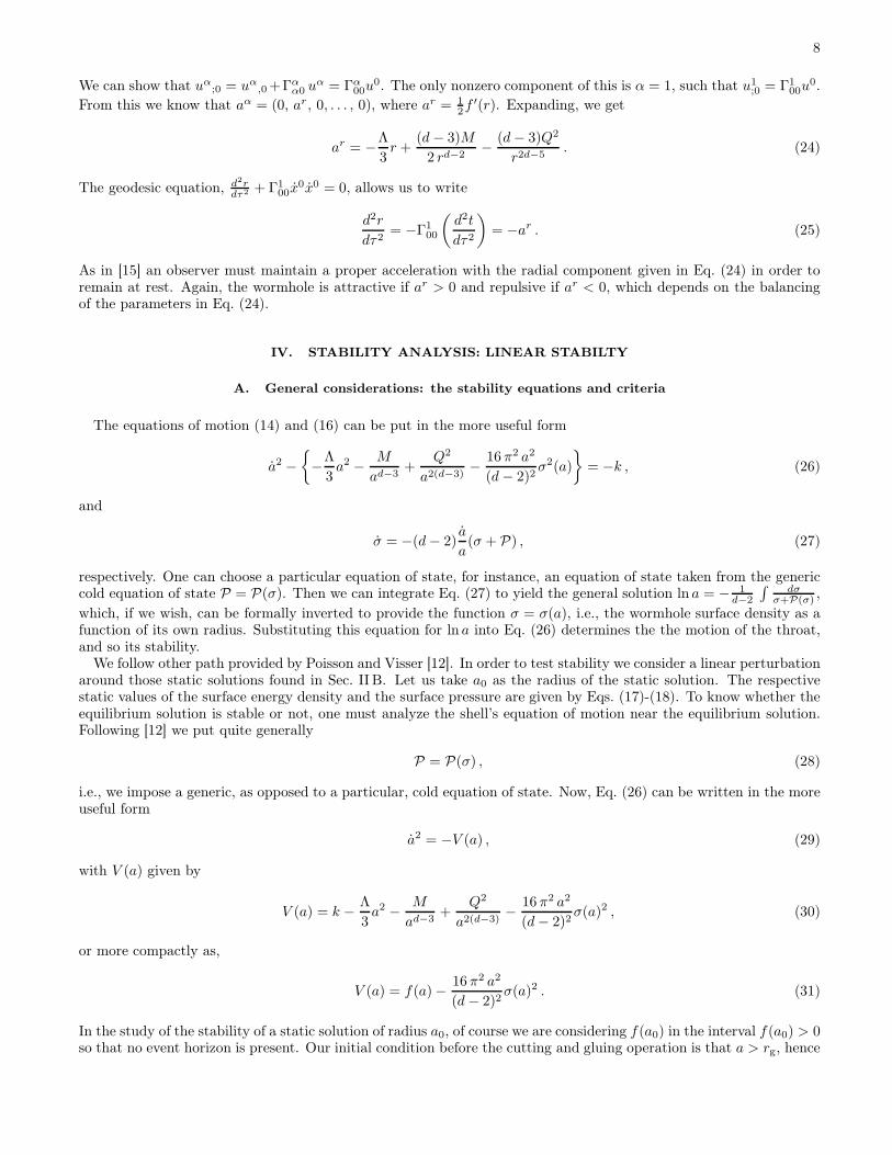
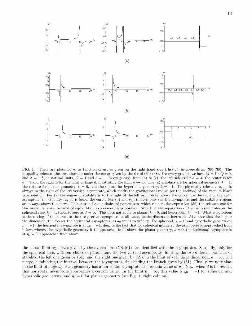
In Fig. 1 η0 is plotted as a function of a0 and the regions of stability are displayed in some chosen particular cases,namely, d = 4 , 5 ,∞, k = 1, 0,−1, Λ 6= 0, and Q = 0. For all plots we put further M = 10 and Λ = − 1

5 , in naturalunits, i.e., G = 1 and c = 1. The items (a), (b), and (c) refer to the three possible geometries of the AdS spacetime,namely, k = 1 spherical, k = 0 planar, k = −1 hyperbolic, respectively. For each item ((a), (b), and (c)) we displaythree plots, namely, for d = 4, d = 5, and d = ∞. In the plots, the physically relevant region is always to the right ofthe left vertical asymptote, which marks the gravitational radius (or the horizon) of the solution. Given d, k, M , andΛ, Eqs. (59)-(61) tell us the regions in a plot η0 × a0 where the stability conditions are satisfied. Depending in whichslot of the rhs of (59)-(61) one is, the inequality on the left hand side gives the region above or under the curves ofFig. 1.

For k = 1, Fig. 1(a), there are two intervals worth of mentioning. The first interval is between the left asymptoteand the right asymptote. The region of stability is then above the curve shown. The second interval is to the rightof the right asymptote. The stability region is given below the curve shown. In this interval η0 < 0 for which somejustification can be given, see, e.g., [12]. At the point where (60) holds one gets for stability that η0 = +∞ or η0 = −∞depending on the branch one is.

For k = 0, Fig. 1(b), there is only one interval worth of mentioning. This interval is to the right of the leftasymptote. The region of stability is then above the curve shown and η0 > 0 in this region.

For k = −1, Fig. 1(c), there is also only one interval worth of mentioning. This interval is to the right of the leftasymptote. The region of stability is then above the curve shown and η0 > 0 in this region. The parameter η0 can benegative in this region.

Now in each geometry (a), (b), or (c), for finite d the curves do not change qualitatively, as can be seen displayedin the figure. However if we take the limit d = ∞ we find that interesting things happen. Firstly, the gap between theasymptotes and the curves is reduced, and is the shorter as the dimension d increases. This shows that in this limit,the region of stability is going to be the area limited by the respective asymptotes, both vertical and horizontal, as

13

5 10 15 20a0

-20

-10

10

20

Η0

2 4 6 8 10a0

-7.5

-5

-2.5

2.5

5

7.5

Η0

0.2 0.4 0.6 0.8 1a0

-1.5

-1

-0.5

0.5

1Η0

(a)

5 10 15 20a0

-7.5

-5

-2.5

2.5

5

7.5

Η0

5 10 15 20a0

-2

-1

1

2

3Η0

0.2 0.4 0.6 0.8 1 1.2 1.4a0

-1.5

-1

-0.5

0.5

1

1.5Η0

(b)

5 10 15 20a0

-10

-5

5

10

Η0

5 10 15 20a0

-4

-2

2

Η0

1 2 3 4 5 6a0

-2

-1.5

-1

-0.5

0.5Η0

(c)

FIG. 1: These are plots for η0 as function of a0, as given on the right hand side (rhs) of the inequalities (36)-(38). Theinequality refers to the area above or under the curves given by the rhs of (36)-(38). For every graphic we have M = 10, Q = 0,and Λ = − 1

5, in natural units, G = 1 and c = 1. In every case, from (a) to (c), the left side is for d = 4, the center is for

d = 5 and the right is for the limit of large d, illustrating the limit d → ∞. The (a) graphics are for spherical geometry, k = 1,the (b) are for planar geometry, k = 0, and the (c) are for hyperbolic geometry, k = −1. The physically relevant region isalways to the right of the left vertical asymptote, which marks the gravitational radius (or the horizon) of the vacuum blackhole solution. For (a) the region of stability is to the right of the left asymptote, above the curve. To the right of the rightasymptote, the stability region is below the curve. For (b) and (c), there is only the left asymptote, and the stability regionsare always above the curve. This is true for our choice of parameters, which renders the expression (38) the relevant one forthis particular case, because of eqcondition expression being positive. Note that the separation of the two asymptotes in thespherical case, k = 1, tends to zero as d → ∞. This does not apply to planar, k = 0, and hyperbolic, k = −1. What is notoriousis the closing of the curves to their respective asymptotes in all cases, as the dimension increases. Also note that the higherthe dimension, the clearer the horizontal asymptotes, as a0 tends to infinity. For spherical, k = 1, and hyperbolic geometries,k = −1, the horizontal asymptote is at η0 = −1, despite the fact that for spherical geometry the asymptote is approached frombelow, whereas for hyperbolic geometry it is approached from above; for planar geometry, k = 0, the horizontal asymptote isat η0 = 0, approached from above.

the actual limiting curves given by the expressions (59)-(61) are identified with the asymptotes. Secondly, only forthe spherical case, with our choice of parameters, the two vertical asymptotes, limiting the two different branches ofstability, the left one given by (61), and the right one given by (59), in the limit of very large dimension, d = ∞, willmerge, eliminating the interval between the asymptotes, thus ending the branch given by (61). Finally, we note thatin the limit of large a0, each geometry has a horizontal asymptote at a certain value of η0. Now, when d is increased,this horizontal asymptote approaches a certain value. In the limit d = ∞, this value is η0 = −1 for spherical andhyperbolic geometries, and η0 = 0 for planar geometry (see Fig. 1, right column).

14

V. CONCLUSIONS

We have used the cut and paste procedure in order to build a class of d-dimensional wormholes, with a (d − 1)-dimensional timelike throat, by gluing together the spacetimes of geometric-topological d-dimensional charged vacuumsolutions, with a negative cosmological constant, cut somewhere above the respective gravitational radii. Afterobtaining the static solutions, through the use of the Darmois-Israel formalism, we analyzed the energy conditions,and performed a linearized stability analysis, where the purpose was to establish the response of the solutions to alinear perturbation around a static configuration. We obtained general results. Previous results are obtainable fromthe present’s work general results for the appropriate choices of d, k, Λ and Q.

Acknowledgments

GASD thanks Centro Multidisciplinar de Astrofísica - CENTRA for hospitality. GASD is supported by FCTfellowship SFRH/BPD/63022/2009. This work was partially supported by FCT - Portugal through projectsCERN/FP/109276/2009 and PTDC/FIS/098962/2008.

[1] M. Visser, Lorentzian wormholes: from Einstein to Hawking (AIP Press, New York, 1995).[2] D. Hochberg and M. Visser, Geometric structure of the generic static traversable wormhole throat, Phys. Rev. D 56, 4745

(1997), arXiv:gr-qc/9704082;D. Hochberg and M. Visser, Dynamic wormholes, antitrapped surfaces, and energy conditions, Phys. Rev. D 58, 044021(1998), arXiv:gr-qc/9802046;C. Barcelo and M. Visser, Twilight for the energy conditions?, Int. J. Mod. Phys. D 11, 1553 (2002), arXiv:gr-qc/0205066;M. Visser, S. Kar, and N. Dadhich, Traversable wormholes with arbitrarily small energy condition violations, Phys. Rev.Lett. 90, 201102 (2003), arXiv:gr-qc/0301003;S. Kar, N. Dadhich, and M. Visser, Quantifying energy condition violations in traversable wormholes, Pramana 63, 859(2004), arXiv:gr-qc/0405103.

[3] H. G. Ellis, Ether flow through a drainhole: A particle model in general relativity, J. Math. Phys. (N.Y.) 14, 104 (1973);K. A. Bronnikov, Scalar-tensor theory and scalar charge, Acta Phys. Pol. B 4, 251 (1973);T. Kodama, General-relativistic nonlinear field: a kink solution in a generalized geometry, Phys. Rev. D. 18, 3529 (1978).

[4] C. Barceló and M. Visser, Traversable wormholes from massless conformally coupled scalar fields, Phys. Lett. B 466, 127(1999), arXiv:gr-qc/9908029;C. Barceló and M. Visser, Scalar fields, energy conditions and traversable wormholes, Classical Quantum Gravity 17, 3843(2000), arXiv:gr-qc/0003025;S. V. Sushkov and S.-W. Kim, Wormholes supported by a kink-like configuration of a scalar field, Classical Quantum Grav-ity 19, 4909 (2002), arXiv:gr-qc/0208069;T. A. Roman, Inflating Lorentzian wormholes, Phys. Rev. D. 47, 1370 (1993), arXiv:gr-qc/9211012;M. Cataldo, S. del Campo, P. Minning, and P. Salgado, Evolving Lorentzian wormholes supported by phantom matter andcosmological constant, Phys. Rev. D 79, 024005 (2009), arXiv:0812.4436 [gr-qc];L.-X. Li, Two open universes connected by a wormhole: exact solutions, Journ. Geom. Phys. 40, 154 (2001),arXiv:hep-th/0102143;D. Hochberg, A. Popov, and S. V. Sushkov, Self-consistent wormhole solutions of semiclassical gravity, Phys. Rev. Lett.78, 2050 (1997), arXiv:gr-qc/9701064;K. K. Nandi, B. Bhattacharjee, S. M. K. Alam, and J. Evans, Brans-Dicke wormholes in the Jordan and Einstein frames,Phys. Rev. D 57, 823 (1998), arXiv:0906.0181 [gr-qc];K. A. Bronnikov and S. W. Kim, Possible wormholes in a brane world, Phys. Rev. D 67, 064027 (2003),arXiv:gr-qc/0212112;M. La Camera, Wormhole solutions in the Randall-Sundrum scenario, Phys. Lett. B 573, 27 (2003), arXiv:gr-qc/0306017;F. S. N. Lobo, General class of braneworld wormholes, Phys. Rev. D 75, 064027 (2007), arXiv:gr-qc/0701133;S. V. Sushkov, Wormholes supported by a phantom energy, Phys. Rev. D 71, 043520 (2005), arXiv:gr-qc/0502084;A. Das and S. Kar, The Ellis wormhole with tachyon matter, Classical Quantum Gravity 22, 3045 (2005),arXiv:gr-qc/0505124;A V. B. Arellano and F. S. N. Lobo, Evolving wormhole geometries within nonlinear electrodynamics, Classical QuantumGravity 23, 5811 (2006), arXiv:gr-qc/0608003;A. V. B. Arellano and F. S. N. Lobo, Traversable wormholes coupled to nonlinear electrodynamics, Classical QuantumGravity 23, 7229 (2006), arXiv:gr-qc/0604095;A. B. Balakin, S. V. Sushkov, and A. E. Zayats, Nonminimal Wu-Yang wormhole, Phys. Rev. D 75, 084042 (2007),arXiv:0704.1224 [gr-qc];K. A. Bronnikov and S. Grinyok, Charged wormholes with nonminimally coupled scalar fields, existence and stability,

15

arXiv:gr-qc/0205131;J. A. Gonzalez, F. S. Guzman, and O. Sarbach, On the instability of charged wormholes supported by a ghost scalar field,Phys. Rev. D 80, 024023 (2009), arXiv:0906.0420;A. B. Balakin, J. P. S. Lemos, and A. E. Zayats, Nonminimal coupling for the gravitational and electromagnetic fields:Traversable electric wormholes, Phys. Rev. D 81, 064012 (2010); arXiv:0904.1741 [gr-qc];K. A. Bronnikov, J. P. S. Lemos Cylindrical wormholes, Phys. Rev. D 79, 104019 (2009); arXiv:0902.2360 [gr-qc].

[5] K. A. Bronnikov, S. V. Grinyok, Instability of wormholes with a nonminimally coupled scalar field, Grav. Cosmol. 7, 297(2001), arXiv:gr-qc/0201083;K. A. Bronnikov, S. V. Grinyok, Conformal continuations and wormhole instability in scalar-tensor gravity, Grav. Cosmol.10, 237 (2004), arXiv:gr-qc/0411063;K. A. Bronnikov, S. V. Grinyok, Electrically charged and neutral wormhole instability in scalar-tensor gravity, Grav.Cosmol. 11, 75 (2005), arXiv:gr-qc/0509062.

[6] M. S. Morris and K. S. Thorne, Wormholes in spacetime and their use for interstellar travel: A tool for teaching generalrelativity, Am. J. Phys. 56, 395 (1988);M. Morris, K. S. Thorne, and U. Yurtsever, Wormholes, time machines and the weak energy condition, Phys. Rev. Lett.61, 1446 (1988).

[7] J. P. S. Lemos, F. S. N. Lobo, and S. Quinet de Oliveira, Morris -Thorne wormholes with a cosmological constant Phys.Rev. D 68, 064004 (2003); arXiv:gr-qc/0302049].

[8] M. S. R. Delgaty and R. B. Mann, Traversable wormholes in (2+1) and (3+1) dimensions with a cosmological constant,Int. J. Mod. Phys. D 4, 231 (1995), arXiv:gr-qc/9404046;L. A. Anchordoqui and S. E. Perez Bergliaffa, Wormhole surgery and cosmology on the brane: The world is not enough,Phys. Rev. D 62, 067502 (2000), arXiv:gr-qc/0001019;F. S. N. Lobo, Phantom energy traversable wormholes, Phys. Rev. D 71, 084011 (2005), arXiv:gr-qc/0502099;F. S. N. Lobo, Chaplygin traversable wormholes, Phys. Rev. D 73, 064028 (2006), arXiv:gr-qc/0511003;F. S. N. Lobo, Van der Waals quintessence stars, Phys. Rev. D 75, 024023 (2007), arXiv:gr-qc/0610118.

[9] F. S. N. Lobo, Stability of phantom wormholes, Phys. Rev. D 71, 124022 (2005), arXiv:gr-qc/0506001.[10] M. Visser, Traversable wormholes: Some simple examples, Phys. Rev. D 39 (1989) 3182;

M. Visser, Traversable wormholes from surgically modified Schwarzschild space-times, Nucl. Phys. B 328 (1989) 203.[11] S. W. Kim, Schwarzschild-De Sitter type wormhole, Phys. Lett. A 166, 13 (1992);

F. S. N. Lobo, Surface stresses on a thin shell surrounding a traversable wormhole, Class. Quant. Grav. 21, 4811 (2004),arXiv:gr-qc/0409018;J. P. S. Lemos and F. S. N. Lobo, Plane symmetric traversable wormholes in an anti-de Sitter background, Phys. Rev. D69, 104007 (2004), arXiv:gr-qc/0402099;E. F. Eiroa and C. Simeone, Cylindrical thin-shell wormholes, Phys. Rev. D 70, 044008 (2004), arXiv:gr-qc/0404050;E. F. Eiroa and C. Simeone, Thin-shell wormholes in dilaton gravity, Phys. Rev. D 71, 127501 (2005), arXiv:gr-qc/0502073;M. Thibeault, C. Simeone, and E. F. Eiroa, Thin-shell wormholes in Einstein-Maxwell theory with a Gauss-Bonnet term,Gen. Rel. Grav. 38, 1593 (2006), arXiv:gr-qc/0512029;F. Rahaman, M. Kalam, and S. Chakraborty, Thin shell wormholes in higher dimensional Einstein-Maxwell theory, Gen.Rel. Grav. 38, 1687 (2006), arXiv:gr-qc/0607061;C. Bejarano, E. F. Eiroa, and C. Simeone, Thin-shell wormholes associated with global cosmic strings, Phys. Rev. D 75,027501 (2007), arXiv:gr-qc/0610123;F. Rahaman, M. Kalam, and S. Chakraborty, Thin shell wormhole in heterotic string theory, Int. J. Mod. Phys. D 16,1669 (2007), arXiv:gr-qc/0611134;F. Rahaman, M. Kalam, K. A. Rahman, and S. Chakraborty, A theoretical construction of a thin shell wormhole from atidal charged black hole, Gen. Rel. Grav. 39, 945 (2007) arXiv:gr-qc/0703143;E. Gravanis and S. Willison, ‘Mass without mass’ from thin shells in Gauss-Bonnet gravity, Phys. Rev. D 75, 084025(2007), arXiv:gr-qc/0701152;H. Maeda and M. Nozawa, Static and symmetric wormholes respecting energy conditions in Einstein-Gauss-Bonnet gravity,Phys. Rev. D 78, 024005 (2008), arXiv:0803.1704 [gr-qc];M. G. Richarte and C. Simeone, Traversable wormholes in a string cloud, Int. J. Mod. Phys. D 17, 1179 (2008);arXiv:0711.2297 [gr-qc].

[12] E. Poisson and M. Visser, Thin-shell wormholes: Linearization stability, Phys. Rev. D 52 7318 (1995), arXiv:gr-qc/9506083.[13] F. S. N. Lobo and P. Crawford, Linearized stability analysis of thin-shell wormholes with a cosmological constant, Class.

Quant. Grav. 21, 391 (2004), arXiv:gr-qc/0311002.[14] E. F. Eiroa and G. E. Romero Linearized stability of charged thin-shell wormholes, Gen. Rel. Grav. 36 651-659 (2004),

arXiv:gr-qc/0303093.[15] J. P. S. Lemos and F. S. N. Lobo, Plane symmetric thin-shell wormholes: solutions and stability, Phys. Rev D 78, 044030

(2008), arXiv:0806.4459 [gr-qc].[16] F. Rahaman, M. Kalam, and S. Chakraborty, Thin shell wormholes in higher dimensional Einstein-Maxwell theory, Gen.

Relativ. Gravit. 38, 1687 (2006), arXiv:gr-qc/0607061 .[17] E. F. Eiroa and C. Simeone, Stability of Chaplygin gas thin-shell wormholes, Phys. Rev. D 76, 024021 (2007)

arXiv:0704.1136 [gr-qc];E. F. Eiroa, Stability of thin-shell wormholes with spherical symmetry, Phys. Rev. D 78, 024018 (2008), arXiv:0805.1403[gr-qc];

16

A. A. Usmani, F. Rahaman, S. Ray, Sk. A. Rakib, and Z. Hasan, Thin-shell wormholes from charged black holes in gener-alized dilaton-axion gravity, Gen. Rel. Grav., to appear (2010), arXiv:1001.1415 [gr-qc];P. K. F. Kuhfittig, The stability of thin-shell wormholes with a phantom-like equation of state, Acta Phys. Polonica B, toappear (2010), arXiv:1008.3111 [gr-qc];E. F. Eiroa and C. Simeone, Some general aspects of thin-shell wormholes with cylindrical symmetry, Phys. Rev. D 81,084022 (2010), arXiv:0912.5496 [gr-qc] (2009).

[18] M. Ishak and K. Lake, Stability of transparent spherically symmetric thin shells and wormholes, Phys. Rev. D 65, 044011(2002), arXiv:gr-qc/0108058;F. S. N. Lobo and P. Crawford, Stability analysis of dynamic thin shells, Class. Quant. Grav. 22, 4869 (2005),arXiv:gr-qc/0507063.

[19] N. Arkani-Hamed, S. Dimopoulos, and G. Dvali, The hierarchy problem and new dimensions at a millimeter, Phys. Lett.B 429, 263 (1998), arXiv:hep-ph/9803315;L. Randall and R. Sundrum, An alternative to compactification, Phys. Rev. Lett. 83, 4690 (1999), arXiv:hep-th/9906064.

[20] S. Weinberg, The cosmological constant problem, Rev. Mod. Phys. 61, 1 (1989);O. Lahav, A. R. Liddle, The cosmological parameters 2010, The Review of Particle Physics 2010 (the Particle Data Book),arXiv:1002.3488 [astro-ph];G. W. Gibbons, Anti de Sitter spacetime and its uses, in Mathematical and quantum aspects of relativity and cosmology(Proceedings of the second Samos meeting on cosmology, geometry and relativity), Pythagorean, Samos, Greece 1998, eds.S. Cotsakis and G. W. Gibbons (Springer, Berlin 2000), p. 102;O. Aharony, S. S. Gubser, J. M. Maldacena, H. Ooguri, and Y. Oz, Large N field theories, string theory and gravity, Phys.Rept. 323, 183 (2000), arXiv:hep-th/9905111;S. Kachru, R. Kallosh, A. Linde, and S. P. Trivedi, de Sitter vacua in string theory, Phys. Rev. D 68,046005 (2003),arXiv:hep-th/0301240.

[21] J. P. S. Lemos, Two-dimensional black holes and planar general relativity, Class. Quantum Grav. 12, 1081 (1995),arXiv:gr-qc/9407024;J. P. S. Lemos, Cylindrical black Hole in general relativity, Phys. Lett. B353, 46 (1995), arXiv:gr-qc/9404041;J. P. S. Lemos and V. T. Zanchin, Rotating charged black strings in general relativity Phys. Rev. D 54, 3840 (1996),arXiv:hep-th/9511188;R. B. Mann, Pair production of topological anti-de Sitter black holes, Class. Quantum Grav. 14, L109 (1997),arXiv:gr-qc/9607071;D. Birmingham, Topological black holes in anti-de Sitter space, Class. Quant. Grav. 16, 1197 (1999), arXiv:hep-th/9812206;J. P. S. Lemos, Black holes with toroidal, cylindrical and planar horizons in anti-de Sitter spacetimes in general relativityand their properties, in Astronomy and Astrophysics: Recent Developments, Proceedings of the 10th Astronomy and As-trophysics meeting, ed. A. Mourao et al (World Scientific, 2001), p. 88, arXiv:gr-qc/0011092;N. L. Santos, O. J. C. Dias, and J. P. S. Lemos, Global embedding of D-dimensional black holes with a cosmologicalconstant in Minkowskian spacetimes: Matching between Hawking temperature and Unruh temperature, Phys. Rev. D 70,124033 (2004), arXiv:hep-th/0412076;A. DeBenedictis, Developments in black hole research: Classical, semi-classical, and quantum, Classical and QuantumGravity Research (Nova Sci. Pub. 2008), p. 371, arXiv:0711.2279 [gr-qc];F. C. Mena, J. Natario, and P. Tod, Formation of Higher-dimensional Topological Black Holes, Ann. Inst. Henri Poincaré10, 1359 (2010), arXiv:0906.3216 [gr-qc].

[22] C. W. Misner and J. A. Wheeler, Classical physics as geometry: Gravitation, electromagnetism, unquantized charge, andmass as properties of curved empty space, Ann. of Phys. 2, 525 (1957);J. A. Wheeler, On the nature of quantum geometrodynamics, Ann. of Phys. 2, 604 (1957);M. D. Kruskal, Maximal extension of Schwarzschild metric, Phys. Rev. 119, 1743 (1960);J. C. Graves and D. R. Brill, Oscillatory character of Reissner-Nordström metric for an ideal charged wormhole, Phys.Rev. 120, 1507 (1960).