Three-dimensional photon counting integral imaging using Bayesian estimation

Three-dimensional photon counting integral

imaging reconstruction using penalized

maximum likelihood expectation maximization

Doron Aloni,1 Adrian Stern,1,* and Bahram Javidi2 1Electro Optical Unit, Ben Gurion University of the Negev, Beer-Sheva 84105, Israel

2Dept. of Electrical and Computer Engineering, University of Connecticut, Storrs, Connecticut 06269-2157 USA

*[email protected]

Abstract: Recent works have demonstrated that three-dimensional (3D)

object reconstruction is possible from integral images captured in

severely photon starved conditions. In this paper we propose an iterative

approach to implement a maximum likelihood expectation

maximization estimator with several types of regularization for 3D

reconstruction from photon counting integral images. We show that the

proposed algorithms outperform the previously reported approaches for

photon counting 3D integral imaging reconstruction. To the best of our

knowledge, this is the first report on using iterative statistical

reconstruction techniques for 3D photon counting integral imaging.

©2011 Optical Society of America

OCIS codes: (100.3010) Image reconstruction techniques; (110.6880) Three-dimensional

image acquisition; (100.6890) Three-dimensional image processing; (110.1758)

Computational imaging; (030.5260) Photon counting.

References and links

1. A. Stern and B. Javidi, “Three dimensional image sensing, visualization, and processing using integral

imaging,” Proc. IEEE 94(3), 591–607 (2006).

2. G. Lippmann, “La photographie integrale,” C. R. Acad. Sci. 146, 446–451 (1908).

3. B. Javidi, R. Ponce-Díaz, and S.-H. Hong, “Three-dimensional recognition of occluded objects by using

computational integral imaging,” Opt. Lett. 31(8), 1106–1108 (2006).

4. B. Javidi, F. Okano, and J.-Y. Son, eds., Three-Dimensional Imaging, Visualization, and Display (Springer,

2008).

5. T. Okoshi, “Three-dimensional displays,” Proc. IEEE 68(5), 548–564 (1980). 6. H. Hoshino, F. Okano, H. Isono, and I. Yuyama, “Analysis of resolution limitation of integral

photography,” J. Opt. Soc. Am. A 15(8), 2059–2065 (1998).

7. R. Martinez-Cuenca, G. Saavedra, M. Martinez-Corral, and B. Javidi, “Progress in 3-D multiperspective display by integral imaging,” Proc. IEEE 97(6), 1067–1077 (2009).

8. M. C. Forman, N. Davies, and M. McCormick, “Continuous parallax in discrete pixelated integral three-

dimensional displays,” J. Opt. Soc. Am. A 20(3), 411–420 (2003). 9. F. Okano, J. Arai, K. Mitani, and M. Okui, “Real-time integral imaging based on extremely high resolution

video system,” Proc. IEEE 94(3), 490–501 (2006).

10. B. Javidi, S.-H. Hong, and O. Matoba, “Multidimensional optical sensor and imaging system,” Appl. Opt.

45(13), 2986–2994 (2006).

11. H. Arimoto and B. Javidi, “Integral three-dimensional imaging with digital reconstruction,” Opt. Lett. 26(3),

157–159 (2001).

12. S. Yeom, B. Javidi, and E. Watson, “Photon counting passive 3D image sensing for automatic target

recognition,” Opt. Express 13(23), 9310–9330 (2005).

13. B. Tavakoli, B. Javidi, and E. Watson, “Three dimensional visualization by photon counting computational Integral Imaging,” Opt. Express 16(7), 4426–4436 (2008).

14. J. Jung, M. Cho, D. K. Dey, and B. Javidi, “Three-dimensional photon counting integral imaging using

Bayesian estimation,” Opt. Lett. 35(11), 1825–1827 (2010). 15. I. Moon and B. Javidi, “Three dimensional imaging and recognition using truncated photon counting model

and parametric maximum likelihood estimator,” Opt. Express 17(18), 15709–15715 (2009).

16. I. Moon and B. Javidi, “Three-dimensional recognition of photon-starved events using computational integral imaging and statistical sampling,” Opt. Lett. 34(6), 731–733 (2009).

17. J. W. Goodman, Statistical Optics (Wiley, 1985).

18. M. Bertero, P. Boccacci, G. Desidera, and G. Vicidomini, “Image deblurring with Poisson data: from cells

to galaxies,” Inverse Probl. 25(12), 123006 (2009).

19. R. M. Lewitt and S. Matej, “Overview of methods for image reconstruction from projections in emission

computed tomography,” Proc. IEEE 91(10), 1588–1611 (2003).

#147440 - $15.00 USD Received 16 May 2011; revised 22 Aug 2011; accepted 29 Aug 2011; published 23 Sep 2011(C) 2011 OSA 26 September 2011 / Vol. 19, No. 20 / OPTICS EXPRESS 19681

20. S. Geman and D. Geman, “Stochastic relaxation, Gibbs distributions and Baysesian restoration of images,”

IEEE Trans. Pattern Anal. Mach. Intell. PAMI-6(6), 721–741 (1984). 21. S. Alenius and U. Ruotsalainen, “Generalization of median root prior reconstruction,” IEEE Trans. Med.

Imaging 21(11), 1413–1420 (2002).

22. V. Y. Panin, G. L. Zeng, and G. T. Gullberg, “Total variation regulated EM algorithm [SPECT reconstruction],” IEEE Trans. Nucl. Sci. 46(6), 2202–2210 (1999).

23. N. Dey, L. Blanc-Feraud, C. Zimmer, P. Roux, Z. Kam, J. C. Olivo-Marin, and J. Zerubia, “Richardson-

Lucy algorithm with total variation regularization for 3D confocal microscope deconvolution,” Microsc.

Res. Tech. 69(4), 260–266 (2006).

1. Introduction

Integral imaging [1–16] (InI) is an autostereoscopic three-dimension (3D) passive

imaging technique originally proposed by G. Lippmann [2] a century ago and was revived

in the last decade due to advances in digital imaging technology and optical and

optoelectronic devices. Sensing of the 3D scene is carried out by capturing elemental

images optically using a pickup microlens array and a detector array (Fig. 1) or by using

multiple cameras. Integral imaging acquisition may be viewed as a multichannel system

[1] where each channel generates an elemental image (EI). As such, there is a large

redundancy in the captured data permitting visualization of occluded objects [3], 3D

target recognition [1], and 3D image restoration in photon starved conditions [12–16]. 3D

object reconstruction can be performed either optically or computationally. Optical

reconstruction is depicted in Fig. 1(b). Computational reconstruction typically mimic the

optical reconstruction, however has the additional flexibility of digitally manipulating the

data to extract better visual information [1]. In this paper we address the problem of

computationally visualizing 3D objects from photon counting integral images. Following

the work by Yeom et al. [12] demonstrating the possibility to recognize 3D object from

InI with very small photon counts per elemental image, several approaches for extracting

the visual information from InI captured in photon starved environments have been

introduced [13–16]. In Ref. [13] Maximum Likelihood Estimation (MLE) with Poisson

distribution was used for 3D passive sensing and visualization using InI for 3D image

reconstruction· The photon counting detection model [17] was used to reconstruct 3D

objects from photon counting images. Although MLE produced reasonably good results,

simple MLE cannot provide optimal reconstruction because no prior information about

the object is exploited. A follow up study [14] used Bayesian estimation with Gamma

distribution as prior. This estimator is also not optimal since Gamma prior may not

necessarily be the best way to describe object characteristics. Another study [15]

considered truncated Poisson distribution which describes more accurately the photon

counting conditions at extremely low photon, however it lacks an efficient way to include

prior constrains.

In this work, we propose to reconstruct photon counting InI by using several penalized

maximum likelihood expectation maximization (PMLEM) algorithms. In general,

PMLEM algorithms effectively combines the Poisson statistics model associated with

photon counting process, with penalties reflecting prior information or assumptions about

the image (e.g., see [18] and references therein). MLEM algorithms were found to be very

useful in various photon starved imagery, such as astronomy [18], nuclear medicine (e.g.,

Refs. [19–22]), and microscopy [23]. Here we demonstrate its effectiveness in photon

counting integral-imaging.

The paper is organized as following. In section 2 we briefly overview the 3D integral

imaging; we present the PMLEM algorithm and explain its implementation in photon

counting integral imaging. Then, in section 3, experimental results will be presented

followed by concluding remarks in section 4.

2. Integral imaging with penalized maximum likelihood expectation maximization

reconstruction

2.1 Reconstruction algorithms

Integral imaging (InI) is a three-dimensional (3D) imaging technique that can sense a 3D

scene and reconstruct it as a 3D volumetric image. The InI acquisition scheme is depicted


Fig. 1. (a) forward projection of a 3D object in the InI plane through microlens array. (b)

Backward projection.

in Fig. 1. The reconstruction of the 3D object can be carried out optically or

computationally [1,13]. Typically, computational reconstruction of volume pixels of the

scene is accomplished by numerically simulating the optical reconstruction process; that

is, by back propagating the captured light rays in Fig. 1(b). Image depth planes at arbitrary

distances from the display microlens array are reconstructed by back propagating the

elemental images (multi-view images) through a virtual pinhole array following ray optics

[1,13]:

( )1 1

0

0 0 0 0

1 1 1. . ,

K LBP

kl x y

k l

f x y z g x S k y S lKL M M

− −

= =

= + +

∑∑ (1)

where BPf is the reconstruction image at a specific depth plane and g represents the

elemental images, xS and yS are the shifting factor between each lens at x and y

directions respectively, K and L represent the number of elemental images at the CCD

plane, k and l are indexes that pointing the pixel at such elemental image. For object

located at distance z = 0z from the lens of the imaging device,

0M is the magnification

factor.

Algebraically, relation (1) can be expressed as

BP T= ⋅f A g (2)

where BPf is a lexicographic vector representing backprojected reconstruc-

tion, [ ]( ),BP

vect f n m=f , and g is a lexicographic vector representing the elemental

images at the CCD plane. TA is the adjoin of the forward projection operator A defining

the relation between the captured image g and the object f:

= ⋅g A f (3)

Algebraically, operator A is an m n× matrix, where m is the total number of pixels in

the captured InI and n is the total number of object pixels. A and AT express the ray

relation between the object and the InI (Fig. 1). We note that back propagation model

expressed by Eq. (1) holds in the geometrical approximation. In case that diffraction and

aberrations are significant it can be easily generalized by accounting for local point spread

function in A.

Equation (2) holds for the noiseless case. However, in low photon acquisition mode,

the measurement vector g is subject to variations due to Poisson noise from the discrete

nature of the arrival of the photon detection [13–16]. Since variance of a Poisson random

variable equals to its mean, at low photon counts the noise added to g in Eq. (2) is

significant. Our goal is to estimate the original 3D image f from g corrupted by Poisson

noise. A well-known iterative solution for this problem is the PMLEM algorithm [18–23]:

( )β

+ = ⋅ ⋅⋅+ ⋅

(k)(k 1) T

(k)k

f gf A

A fs Pf (4)


where TA is the adjoin operator of A representing the backward projection, β is a

constant number controlling the amount of regularization induced by operator P . js is

the sensitivity vector with elements given by ,

1

, 1,...m

j i j

i

s a j n=

= =∑ where ai,j is the i,jth

element of the matrix A; hence js is the sum of the jth object point response in the InI

plane accounting for the number of EIs contributing to reconstruction of the point. The

division in Eq. (4) should be taken as Hadamarad division (component-wise division).

It is noted that in the case β = 0 Eq. (4) represents the MLEM [18] algorithm:

ˆ

ˆ ,ˆ

+ = ⋅ ⋅⋅

(k)(k 1) T

(k)j

f gf A

s A f (5)

which, for a well-conditioned A matrix, reduces to the well-known Richardson-Lucy

deconvolution algorithm [18].

It can be seen that PMLEM algorithm in Eq. (4) uses the forward projection operator

as well as the backward projection operator to estimate iteratively the scene based on the

measurements. They can be seen as a set of successive projections and backprojections

where the factorˆ⋅ (k)

g

A f is the ratio between the captured image- g , and the one that

would be obtained from the estimated object- ˆˆ = ⋅(k) (k)g A f at the kth iteration step. We

notice that any positive initial guess (0)f yields a non-negative guess ˆ (k)f .

Since the acquisition is ill posed the reconstruction process needs to be regularized.

This is done by including the term ( )ˆβ ⋅ kPf in the dominator of Eq. (4). This term

penalizes the (k + 1)th guess according to the penalty operator P controlled by the

parameter b. Penalty P is designed to reflect some prior assumption about the object, such

as local smoothness of f(x,y). Consequently it is calculated on a patch surrounding the

estimated pixel (k)

i, jf . The operator P is applied on the previous guess f(k)

, therefore the

approach is called one-step-late [19].

For regularization of the MLEM algorithm applied for the photon counting integral

imaging, we choose to investigate penalties implementing three types of priors: quadratic

prior, median root prior, and total-variation prior.

2.2 PMLEM with quadratic prior

Probably the most direct prior for imposing smoothness on the image is the quadratic

prior for which the penalty is given by [20]

( ) ( ){ } ( ) ( )( ),

2

, ,

,

ˆ ˆ ˆ ˆ[ , ] [ , ] [ , ]i j

k k k k

i j i j

r s S

f f i j w f i j f i r j s∈

= = − + +∑P P (6)

where Si,j is a set of pixel in the neighborhood of pixel ( )ˆ [ , ]k

f i j , and ,i jw is a weighting

function depending on the distance from the pixel.

2.3 Median root prior

Median root prior assumes that the image is locally smooth such that it passes unaltered

through the median filter. This prior is introduced in the PMLEM by the nonlinear

operator [21]:

( ) ( ){ }

( ) ( ){ }( ){ }

,

,

,

ˆ ˆ[ , ] [ , ];ˆ ˆ [ , ]

ˆ [ , ];

k k

i jk k

i j k

i j

f i j Med f i j Sf f i j

Med f i j S

−= =P P (7)

where { },[ , ]; i jMed f i j S is a median filter applied on a window Si,j in the neighborhood

of pixel [ , ]f i j .


2.4 Total variation average penalty

Minimum total-variation is known as an effective prior for edge preserving regularization.

An expression for the total variation penalty for PMLEM is derived in [22]:

[ ]{ }( ) [ ] ( ) [ ]

[ ]

( ) [ ] ( ) [ ][ ]

( ) [ ] ( ) [ ] ( ) [ ][ ]

,

ˆ ˆ ˆ ˆ, 1, , , 1ˆ ˆ ,1, , 1

ˆ ˆ ˆ1, , 1 2 ,.

,

k k k k

i j

k k k

f i j f i j f i j f i jf f i j

u i j u i j

f i j f i j f i j

u i j

− − − −= = + −

− −

+ + + −

P P

(8)

where

( ) ( ) ( )( ) ( ) ( )( )2 2ˆ ˆ ˆ ˆ[ 1, ] [ , ] [ , 1] [ , ] .

k k k ku i, j f i j f i j f i j f i j ε= + − + + − +

The parameter ε is an artificial parameter to ensure convergence, typically chosen to

be less than 1% [22]. The total-variation constrain has been used extensively in image

processing and it was previously proposed to penalizing the MLE algorithm for nuclear

medicine [19,22] and image reconstruction in microscopy [23].

3. Experimental results

We applied the PMLEM algorithm on real and simulated integral images with the three

penalties mentioned in the previous section. For the quadratic and median penalty we

have Si,j to be a 3x3 window surrounding the pixel [ , ]f i j .

The PMLEM is an iterative algorithm; therefore it requires a stopping condition. The

iterations are stopped when the means square error (MSE) between the estimated image at

iteration k, (k)f , and the previous one −(k 1)f is smaller than a threshold thε ,

2

1

1 1

1 ˆ ˆN M

(k) (k )

i, j i, j th

i j

f fN M

ε−

= =

− ≤⋅ ∑∑ (9)

where N and M are the number of pixels in the x and y coordinates respectively.

Table 1 show representative comparison PSNR results for the three types of penalties

and the un-penalized MLEM. The PSNR is calculated as

,

10

ˆmax( )10log

full

i jPSNR

MSE=

f (10)

where MSE is the mean square error between the reconstructed image from the photon

starved image ˆestf , and the reconstructed image from full photon statistics (i.e., regular

illumination conditions) ˆ fullf :

21

,

full est

i, j i, j

i j

MSE f fi j ROI

= −∈ ∑∑ (11)

where i,j denote the pixel's index in x and y direction, respectively, and ROI is the region

of interest area (i.e., car without background in Fig. 2). Table 1 reveals that total

variations PLMEM (TV-PMLEM) lead to a higher PSNR of about 21.66dB.

Table 1. Reconstruction results with maximum likelihood estimation (MLE),

maximum likelihood expectation maximization (MLEM) and penalized MLEM

(PMLEM) with three types of penalties

THE METHOD PSNR [dB] MLEM 17.5 PMLEM-with quadratic prior 17.72 PMLEM-with median average penalty 20 PMLEM- with total variation average penalty 21.66 MLE 17.68


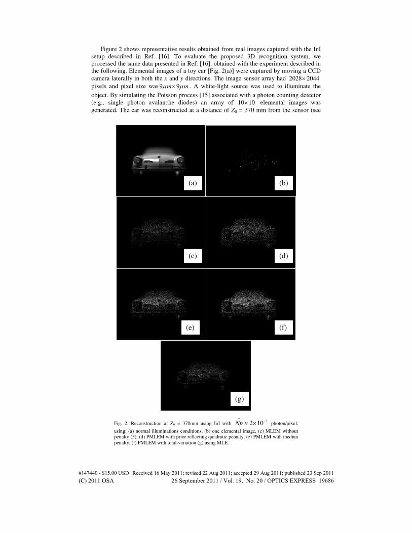
Figure 2 shows representative results obtained from real images captured with the InI

setup described in Ref. [16]. To evaluate the proposed 3D recognition system, we

processed the same data presented in Ref. [16]. obtained with the experiment described in

the following. Elemental images of a toy car [Fig. 2(a)] were captured by moving a CCD

camera laterally in both the x and y directions. The image sensor array had 2028 2044×

pixels and pixel size was 9 9m mµ µ× . A white-light source was used to illuminate the

object. By simulating the Poisson process [15] associated with a photon counting detector

(e.g., single photon avalanche diodes) an array of 10 10× elemental images was

generated. The car was reconstructed at a distance of Z0 = 370 mm from the sensor (see

Fig. 2. Reconstruction at Z0 = 370mm using InI with ~

32 10Np

−≈ × photon/pixel,

using: (a) normal illuminations conditions, (b) one elemental image, (c) MLEM without penalty (5), (d) PMLEM with prior reflecting quadratic penalty, (e) PMLEM with median

penalty, (f) PMLEM with total-variation (g) using MLE.

(a) (b)

(c) (d)

(e) (f)

(g)


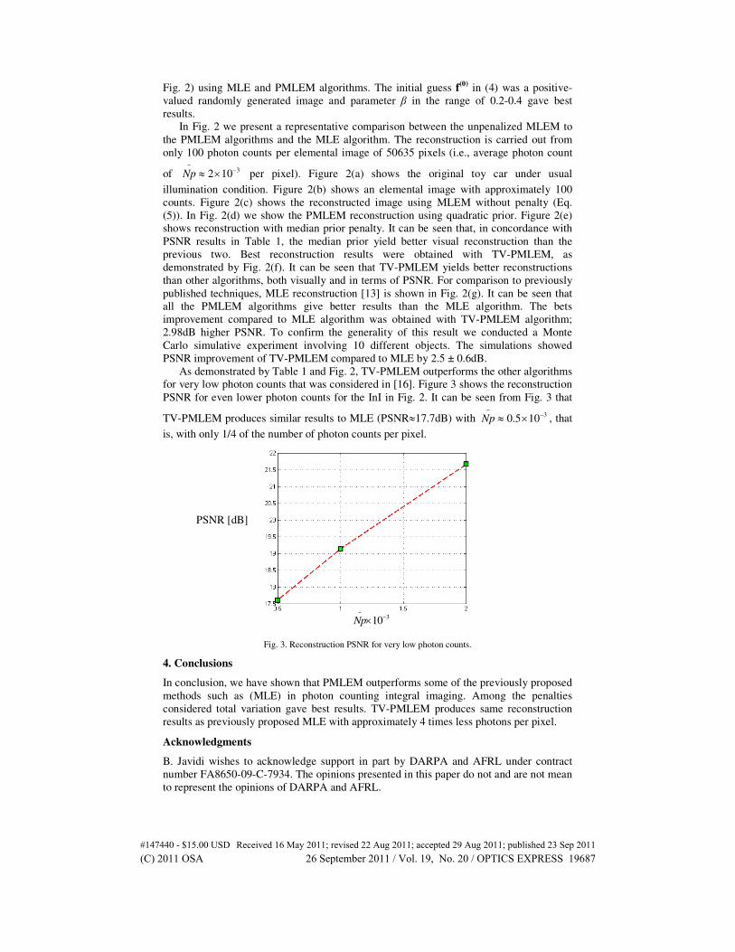
Fig. 2) using MLE and PMLEM algorithms. The initial guess f(0)

in (4) was a positive-

valued randomly generated image and parameter β in the range of 0.2-0.4 gave best

results.

In Fig. 2 we present a representative comparison between the unpenalized MLEM to

the PMLEM algorithms and the MLE algorithm. The reconstruction is carried out from

only 100 photon counts per elemental image of 50635 pixels (i.e., average photon count

of ~

32 10Np−≈ × per pixel). Figure 2(a) shows the original toy car under usual

illumination condition. Figure 2(b) shows an elemental image with approximately 100

counts. Figure 2(c) shows the reconstructed image using MLEM without penalty (Eq.

(5)). In Fig. 2(d) we show the PMLEM reconstruction using quadratic prior. Figure 2(e)

shows reconstruction with median prior penalty. It can be seen that, in concordance with

PSNR results in Table 1, the median prior yield better visual reconstruction than the

previous two. Best reconstruction results were obtained with TV-PMLEM, as

demonstrated by Fig. 2(f). It can be seen that TV-PMLEM yields better reconstructions

than other algorithms, both visually and in terms of PSNR. For comparison to previously

published techniques, MLE reconstruction [13] is shown in Fig. 2(g). It can be seen that

all the PMLEM algorithms give better results than the MLE algorithm. The bets

improvement compared to MLE algorithm was obtained with TV-PMLEM algorithm;

2.98dB higher PSNR. To confirm the generality of this result we conducted a Monte

Carlo simulative experiment involving 10 different objects. The simulations showed

PSNR improvement of TV-PMLEM compared to MLE by 2.5 ± 0.6dB.

As demonstrated by Table 1 and Fig. 2, TV-PMLEM outperforms the other algorithms

for very low photon counts that was considered in [16]. Figure 3 shows the reconstruction

PSNR for even lower photon counts for the InI in Fig. 2. It can be seen from Fig. 3 that

TV-PMLEM produces similar results to MLE (PSNR≈17.7dB) with ~

30.5 10Np−≈ × , that

is, with only 1/4 of the number of photon counts per pixel.

Fig. 3. Reconstruction PSNR for very low photon counts.

4. Conclusions

In conclusion, we have shown that PMLEM outperforms some of the previously proposed

methods such as (MLE) in photon counting integral imaging. Among the penalties

considered total variation gave best results. TV-PMLEM produces same reconstruction

results as previously proposed MLE with approximately 4 times less photons per pixel.

Acknowledgments

B. Javidi wishes to acknowledge support in part by DARPA and AFRL under contract

number FA8650-09-C-7934. The opinions presented in this paper do not and are not mean

to represent the opinions of DARPA and AFRL.

PSNR [dB]

~310Np −×


Documents

Three-dimensional photon counting integral imaging using Bayesian estimation