Embed Size (px)
Citation preview

r>rJfl,>'.)*•
HKra
mitt*
>\
« i
If I * IIT
I
.
I
pI*
.aference nbsPubli-
cations
\
/ %
^mNBS TECHNICAL NOTE 695
U.S. DEPARTMENT OF COMMERCE/National Bureau of Standards
Time and Frequency Users' Manual
100
.U5753
No. 695
1977
NATIONAL BUREAU OF STANDARDS
The National Bureau of Standards 1 was established by an act of Congress March 3, 1901. The Bureau's overall goal is tostrengthen and advance the Nation's science and technology and facilitate their effective application for public benefit To thisend, the Bureau conducts research and provides: (1) a basis for the Nation's physical measurement system, (2) scientific andtechnological services for industry and government, (3) a technical basis for equity in trade, and (4) technical services to pro-mote public safety. The Bureau consists of the Institute for Basic Standards, the Institute for Materials Research the Institutefor Applied Technology, the Institute for Computer Sciences and Technology, the Office for Information Programs, and theOffice of Experimental Technology Incentives Program.
THE INSTITUTE FOR BASIC STANDARDS provides the central basis within the United States of a complete and consist-ent system of physical measurement; coordinates that system with measurement systems of other nations; and furnishes essen-tial services leading to accurate and uniform physical measurements throughout the Nation's scientific community, industry,and commerce. The Institute consists of the Office of Measurement Services, and the following center and divisions:
Applied Mathematics — Electricity — Mechanics — Heat — Optical Physics — Center for Radiation Research — Lab-oratory Astrophysics 2 — Cryogenics 2 — Electromagnetics 2 — Time and Frequency 3
.
THE INSTITUTE FOR MATERIALS RESEARCH conducts materials research leading to improved methods of measure-ment, standards, and data on the properties of well-characterized materials needed by industry, commerce, educational insti-tutions, and Government; provides advisory and research services to other Government agencies; and develops, produces, anddistributes standard reference materials. The Institute consists of the Office of Standard Reference Materials, the Office of Airand Water Measurement, and the following divisions:
Analytical Chemistry — Polymers — Metallurgy — Inorganic Materials — Reactor Radiation — Physical Chemistry.
THE INSTITUTE FOR APPLIED TECHNOLOGY provides technical services developing and promoting the use of avail-able technology; cooperates with public and private organizations in developing technological standards, codes, and test meth-ods; and provides technical advice services, and information to Government agencies and the public. The Institute consists ofthe following divisions and centers:
Standards Application and Analysis — Electronic Technology — Center for Consumer Product Technology: ProductSystems Analysis; Product Engineering — Center for Building Technology: Structures, Materials, and Safety; BuildingEnvironment; Technical Evaluation and Application — Center for Fire Research: Fire Science; Fire Safety Engineering.
THE ENSTITUTE FOR COMPUTER SCIENCES AND TECHNOLOGY conducts research and provides technical servicesdesigned to aid Government agencies in improving cost effectiveness in the conduct of their programs through the selection,acquisition, and effective utilization of automatic data processing equipment; and serves as the principal focus wthin the exec-utive branch for the development of Federal standards for automatic data processing equipment, techniques, and computerlanguages. The Institute consist of the following divisions:
Computer Services — Systems and Software — Computer Systems Engineering — Information Technology.
THE OFFICE OF EXPERIMENTAL TECHNOLOGY INCENTIVES PROGRAM seeks to affect public policy and processto facilitate technological change in the private sector by examining and experimenting with Government policies and prac-tices in order to identify and remove Government-related barriers and to correct inherent market imperfections that impedethe innovation process.
THE OFFICE FOR INFORMATION PROGRAMS promotes optimum dissemination and accessibility of scientific informa-tion generated within NBS; promotes the development of the National Standard Reference Data System and a system of in-
formation analysis centers dealing with the broader aspects of the National Measurement System; provides appropriate services
to ensure that the NBS staff has optimum accessibility to the scientific information of the world. The Office consists of the
following organizational units:
Office of Standard Reference Data — Office of Information Activities — Office of Technical Publications — Library —Office of International Standards — Office of International Relations.
1 Headquarters and Laboratories at Gaithersburg, Maryland, unless otherwise noted; mailing address Washington, D.C. 20234.a Located at Boulder, Colorado 80302.
1 .I C
I
C 1 ! 1977
6 CC-
|9rH
Time and Frequency Users' Manual
Edited by
George Kamas
Time and Frequency Division
Institute for Basic Standards
National Bureau of Standards
Boulder, Colorado 80302
/ W \
V•"•cAU o*
*
U.S. DEPARTMENT OF COMMERCE, Juanita M. Kreps, Secretary
Sidney Harman, Under Secretary
Dr. Betsy Ancker-Johnson, Assistant Secretary for Science and Technology
0$. NATIONAL BUREAU OF STANDARDS, Ernest Ambler, Acting Directoru i
Issued May 1977
NATIONAL BUREAU OF STANDARDS TECHNICAL NOTE 695
Nat. Bur. Stand. (U.S.), Tech Note 695, 217 pages (May 1977)
CODEN: NBTNAE
U.S. GOVERNMENT PRINTING OFFICE
WASHINGTON: 1977
For sale by the Superintendent of Documents, U.S. Government Printing Office, Washington, DC. 20402
CONTENTS
CHAPTER 1. INTRODUCTION: WHAT THIS BOOK IS ABOUT1.1
1 .2
1.3
1.4
1.5
1.6
1.7
1.8
TFTE DEFINITIONS OF TIME AND FREQUENCY
WHAT IS A STANDARD?
1.2.1 Can Time Really Be a Standard?1.2.2 The NBS Standards of Time and Frequency
HOW TIME AND FREQUENCY STANDARDS ARE DISTRIBUTED .
THE NBS ROLE IN INSURING ACCURATE TIME AND FREQUENCYWHEN DOES A MEASUREMENT BECOME A CALIBRATION?TERMS USED
1 .6.1 Mega, Mill i , Parts Per.
1 .6.2 Frequencyand Percents
DISTRIBUTING TIME AND FREQUENCY SIGNALS VIA CABLES AND TELEPHONE LINKS
TIME CODES
PAGE
1
2
3
3
5
5
6
7
7
8
10
12
CHAPTER 2. THE EVOLUTION OF TIMEKEEPING
2.1 TIME SCALES
2.1.1 Solar Time2.1.2 Atomic Time .
A. Coordinated Universal TimeB. The New UTC System .
2.1.3 Time Zones ....2.2 USES OF TIME SCALES ....
2.2.1 Systems Synchronization2.2.2 Navigation and Astronomy
2.3 INTERNATIONAL COORDINATION OF TIME AND FREQUENCY ACTIVITIES
2.3.1 The Role of the International Time Bureau (BIH) .
2.3.2 The Role of the National Bureau of Standards (NBS)
2.3.3 The Role of the U. S. Naval Observatory (USNO) and the DOD PTTI Program
15
15
16
17
17
18
18
18
20
21
21
22
23
CHAPTER 3.
3.43.53.6
THE ALGEBRA AND CONVENTIONS FOR TIME ANDFREQUENCY MEASUREMENTS
3.1 EXPRESSING FREQUENCY DIFFERENCE (IN HERTZ, kHz, MHz, ETC.) .
3-2 RELATIVE (FRACTIONAL) FREQUENCY, F (DIMENS I0NLESS)3.3 RELATIVE (FRACTIONAL) FREQUENCY DIFFERENCE, S (DIMENS I0NLESS)
26
26
27
3.3-1 Example of Algebra and Sign Conventions in Time and Frequency Measurements 27
A. Television Frequency Transfer MeasurementsB. Television Line-10 Time Transfer Measurements
USING TIME TO GET FREQUENCYA MATHEMATICAL DERIVATIONDEFINITIONS
27
28
29
30
31
PAGE
CHAPTER 4. USING TIME AND FREQUENCY IN THE LABORATORY
4.1 ELECTRONIC COUNTERS
4.1.1 Frequency Measurements .
A. Direct Measurement .
B. Prescal ing
C. Heterodyne ConvertersD. Transfer Oscillators
4.1.2 Period Measurements4.1.3 Time Interval Measurements4.1.4 Phase Measurements4.1.5 Pulse-Width Determination Measurements4.1.6 Counter Accuracy ....
A. Time Base ErrorB. Gate Error ....C. Trigger Errors
4.1.7 Printout and Recording .
4.2 OSCILLOSCOPE METHODS ....4.2.1 Calibrating the Oscilloscope Time Base
4.2.2 Direct Measurement of Frequency4.2.3 Frequency Comparisons
A. Lissajous Patterns .
B. Sweep Frequency Calibration: An A
4.2.4 Time Interval Measurements
WAVEMETERSHETERODYNE FREQUENCY METERSDIRECT-READING ANALOG FREQUENCY METERS
4.5.1 Electronic Audio Frequency Meters4.5.2 Radio Frequency Meters .
4.34.4
4.5
4.6
*.7
4.8
4.9
FREQUENCY COMPARATORSAUXILIARY EQUIPMENT .
4.7.1 Frequency Synthesizers .
4.7.2 Phase Error Multipliers4.7.3 Phase Detectors4.7.4 Frequency Dividers
A. Analog or Regenerative D
B. Digital Dividers
4.7.5 Adjustable Rate Dividers4.7.6 Signal Averagers
PHASE LOCK TECHNIQUESSUMMARY
viders
ternative Method
33
35
35
36
36
37
40
42
4344
45
4546
47
50
50
51
52
52
5358
59
5960
62
62
63
63
64
64
65
6567
6768
69
69
70
71
CHAPTER 5. THE USE OF HIGH FREQUENCY BROADCASTS FORTIME AND FREQUENCY CALIBRATIONS
5.1 BROADCAST FORMATS
5.1.1 WWV/WWVH5.1.2 CHU
74
74
75
1 v
PAGE
5.2 RECEIVER SELECTION
5.3 CHOICE OF ANTENNAS AND SIGNAL CHARACTERISTICS5.4 USE OF HF BROADCASTS FOR TIME CALIBRATIONS
5.^.1 Time-of-Day Announcements5.4.2 Using the Seconds Ticks
A. Receiver Time Delay MeasurementsB. Time Delay Over the Radio Path
C. Using an Adjustable Clock to Trigger the OscilloscopeD. Delay Triggering: An Alternate Method that Doesn't
Change the Clock Output ........E. Using Oscilloscope Photography for Greater Measurement Accuracy
5.4.3 Using the WWV/WWVH Time Code
A. Code Format .....B. Recovering the Code
5.5 USE OF HF BROADCASTS FOR FREQUENCY CALIBRATIONS
5.5.1 Beat Frequency Method ....5.5.2 Oscilloscope Lissajous Pattern Method .
5.5.3 Oscilloscope Pattern Drift Method5.5-4 Frequency Calibrations by Time Comparison of Clocks
5.6 FINDING THE PROPAGATION PATH DELAY .
5.6.1 Great Circle Distance Calculations5.6.2 Propagation Delays
5.7 THE NBS TELEPHONE TIME-OF-DAY SERVICE5.8 SUMMARY
76
77
81
81
82
83
83
86
89
89
91
92
93
95
9798
99
99100
104
104
CHAPTER 6. CALIBRATIONS USING LF AND VLF RADIO TRANSMISSIONS
6.1 ANTENNAS FOR USE AT VLF-LF6.2 SIGNAL FORMATS ....6.3 PROPAGATION CHARACTERISTICS AND OTHER PHASE CHANGES6.4 FIELD STRENGTHS OF VLF-LF STATIONS .
6.5 INTERFERENCE6.6 USING WWVB FOR FREQUENCY CALIBRATIONS
6.6.1 Phase-Shift Identification6.6.2 Methods of Frequency Comparison
6.7 USING OTHER LF AND VLF SERVICES FOR FREQUENCY CALIBRATIONS
6.7.1 The Omega Navigation System6.7.2 NLK, NAA, and MSF .
6.8 MONITORING DATA AVAILABILITY .
6.9 USING THE WWVB TIME CODE .
6.9.1 Time Code Format
6.9.2 Time Transfer Using the Transmitted Envelope
105
106
106
110
112
112
113
114
115
115
116
116
116
117
118
6.10 SUMMARY 120
PAGE
CHAPTER 7. FREQUENCY CALIBRATIONS USING TELEVISION SIGNALS
7.1 HOW THIS FITS INTO OTHER NBS SERVICES ....7.2 BASIC PRINCIPLES OF THE TV FREQUENCY CALIBRATION SERVICE
7.2.1 Phase Instabilities of the TV Signals .
7.2.2 Typical Values for the U. S. Networks .
7.3 HOW RELATIVE FREQUENCY IS MEASURED ....7.3.1 Color Bar Comparator .....7.3-2 The NBS System 358 Frequency Measurement Computer
A. Block Diagram Overview ....B. Use of FMC with Unstable Crystal Oscillators
7.4 GETTING GOOD TV CALIBRATIONS
121
122
123
124
126
127
129
130
133
133
CHAPTER 8. FREQUENCY AND TIME CALIBRATIONS USING TV LINE-10
8.1 HOW THE SERVICE WORKS ....8.1.1 Using Line-10 on a Local Basis8.1.2 Using Line-10 for NBS Traceability
8.2 EQUIPMENT NEEDED8.3 TV LINE-10 DATA, WHAT DO THE NUMBERS MEAN?8.4 WHAT DO YOU DO WITH THE DATA? .
8.5 RESOLUTION OF THE SYSTEM .
8.6 GETTING TIME OF DAY FROM LINE-108.7 MEASUREMENTS COMPARED TO THE USNO
8.8 LINE-10 EQUIPMENT AVAILABILITY
135
136
136
138
139140
140
142
142
142
CHAPTER 9. LORAN-C TIME AND FREQUENCY METHODS
9.1 BASIC PRINCIPLES OF THE LORAN-C NAVIGATION SYSTEM
9.1.1 What Is the Extent of Loran-C Coverage?
A. Groundwave Signal RangeB. Skywave Signal Range
9.2 WHAT DO WE GET FROM LORAN-C? .
9.2.1 Signal Characteristics .
9.2.2 Time Setting .
9.2.3 Frequency Calibrations Using Loran-C
9.3 HOW GOOD IS LORAN-C? ....9.3.1 Groundwave Accuracy9.3.2 Skywave Accuracy ....
9.4 ARE THE DATA VALID?
145
147
147
147
148
148
150
152
152
153
154
154
CHAPTER 10. AN INTRODUCTION TO FREQUENCY SOURCES
10.1 FREQUENCY SOURCES AND CLOCKS .
10.2 THE PERFORMANCE OF FREQUENCY SOURCES10.3 USING FREQUENCY STABILITY DATA10.4 RESONATORS10.5 PRIMARY AND SECONDARY STANDARDS
156
158
160
161
163
PAGE
10.6 QUARTZ CRYSTAL OSCILLATORS
10.6.1 Temperature and Aging of Crystals10.6.2 Quartz Crystal Oscillator Performance
10.7 ATOMIC RESONANCE DEVICES
10.7.1 State Selection .......10.7.2 How to Detect Resonance .....10.7.3 Atomic Oscillators ......10.7.4 Atomic Resonator Frequency Stability and Accuracy
10.8 AVAILABLE ATOMIC FREQUENCY DEVICES ....10.8.1 Cesium Beam Frequency Oscillators10.8.2 Rubidium Gas Cell Frequency Oscillators10.8.3 Atomic Hydrogen Masers .....
10.9 TRENDS
164
166
167
168
168
169
172
172
173
173
175
176
177
CHAPTER 11. SUMMARY OF AVAILABLE SERVICES
GLOSSARY
INDEX
179
183
191
TABLES
Table 1.1 PREFIX CONVERSION CHART
Table 1.2 CONVERSIONS FROM PARTS PER... TO PERCENTS
Table 1.3 CONVERSIONS TO HERTZ ....Table ] ,k RADIO FREQUENCY BANDS ....Table 4.1 READINGS OBTAINED WITH VARIOUS SETTINGS OF TIME BASE AND
PERIOD MULTIPLIER CONTROLS .
Table 5-1 HF TIME AND FREQUENCY BROADCAST STATIONS
Table 5.2 IMAGE FREQUENCIES FOR WWV/WWVH
Table 6.1 LF-VLF BROADCAST STATIONS
Table 9.1 U. S. EAST COAST LORAN-C CHAIN
Table 9-2 U. S. WEST COAST LORAN-C CHAIN
Table 9-3 GROUP REPETITION INTERVALS .
Table 10.1 COMPARISON OF FREQUENCY SOURCES
Table 11.1 CHARACTERISTICS OF THE MAJOR T&F DISSEMINATION SYSTEMS
Table 11.2 HOW FREQUENCY IS CALIBRATED
Table 11.3 HOW TIME IS CALIBRATED
7
8
9
9
41
73
77
105
145
146
148
178
179
180
180
VI 1
F gure 1 .1
F gure 1 2
F gure 1 3
F gure 2 1
F gure 2 .2
F gure 2 3
F gure 2 4
F gure 2 5
F gure 2 6
F gure 4 1
F gure 4 2
F gure 4 3
F gure 4 4
F gure 4 5
F' gure 4 6
F gure 4 7
F gure 4 8
F gure 4 9
F gure 4 10
F gure k 11
F gure 4 12
F gure 4 13
F gure 4 14
F gure k 15
F gure 4 16
F gure 4 17
F gure 4 18
F gure 4 19
F gure 4 20
F gure 4 21
F gure 4 22
F gure 4 23
F gure 4 24
F gure 4 25
F gure 4 26
F gure 4 27
F gure 4 28
F gure 4 29
F gure 4 30
F gure 4 31
FIGURES
Organization of the NBS Frequency and Time Standard
IRIG Time Code, Format H
IRIG Time Code Formats
Universal Time Family Relationships
First Atomic Clock.
Classes of Time Scales & Accuracies
Dating of Events in the Vicinity of a Leap Second
Standard Time Zones of the World Referenced to UTC .
NBS, USNO, and BIH Interactions ....Electronic Counters .......Simplified Block Diagram of an Electronic Counter
Diagram of a Counter in the Frequency Measurement Mode
Prescaler-Counter Combination .....Typical Manually-Tuned Heterodyne Converter
Typical Manually-Tuned Transfer Oscillator
Automatic Transfer Oscillators .....Diagram of Counter in the Period-Measurement Mode
Diagram of Counter in the Multiple-Period Mode
Effect of Noise on Trigger Point in Period Measurements
Diagram of Counter in the Time Interval Mode
Optimum Trigger Points for Start-Stop Pulses
Use of Time-Interval Unit for Phase Measurements
Time- I nterva 1 Counter with Start-Stop Channels ConnectedCommon Source for Pulse-Width or Period Measurements
Typical Time Base Stability Curve ....Constant Gating Interval with Ambiguity of +_ 1 Count
Accuracy Chart for Period and Frequency Measurements
Undifferentiated Schmi t
t
_Trigger Waveforms
Time Error Produced by Improper Calibration of Trigger Level Control
Sine Wave Method of Checking Trigger Level Calibration
Digital -to-Analog Arrangement for Chart Recording
Simplified Block Diagram of a Cathode-Ray Oscilloscope
Waveform of Horizontal Deflection Voltage From Time-Base Generator
Time Base Calibration Hookup Using an External Frequency Source
Sine Wave Display as Viewed on Oscilloscope
Equipment Hookup for a 1:1 Lissajous Pattern
to
Elliptical Lissajous Patterns for Two Identical FrequencDifferent Phase .....Development of a 3=1 Lissajous Pattern
Lissajous Patterns ....Arrangement for Measuring Small FrequencyOscilloscope and Frequency Multipliers
Double-Balanced Mixer
Differences with
es of
PAGE
4
12
13
16
16
17
17
19
21
33
3^
35
36
37
38
39
40
41
42
43
43
44
45
46
46
47
48
49
49
50
50
51
51
52
53
53
54
55
56
56
gure k.32
F gure k .33
F "gure 4 .34
F gure 4 .35
F gure 4 .36
F gure 4 .37
F gure 4 38
F gure 4 39
F gure 4 40
F gure 4 41
F gure 4 42
F gure 4 43
F gure 4 44
F gure 4 45
F gure k 46
F gure 4 47
F gure 4 48
F gure 5 1
F gure 5 2
F gure 5 3
F gure 5 4
F gure 5 5
F gure 5 6
F gure 5 7
F gure 5 8
F gure 5 9
F gure 5 10
F gure 5 11
F gure 5 12
F gure 5 13
F gure 5 14
Fi gure 5 15
F gure 5 16
F gure 5 17
F gure 5 18
F gure 5 19
PAGE
Arrangement for Frequency Comparison Using Oscilloscopeand Phase-Error Multiplier ......... 57
Arrangement for Calibrating a Signal Generator ..... 57
Viewing Frequency Drift .......... 58
Wavementer Resonance Indicators ........ 60
Block Diagram of Heterodyne Frequency Meter ...... 61
Arrangement for Checking Transmitting Frequency withHeterodyne Frequency Meter and Receiver ....... 61
Electronic Audio Frequency Meter ........ 62
Direct-Reading Radio Frequency Meter ....... 63
Basic Frequency Comparator ......... 63
Phase Error Multiplier .......... 65
Linear Phase Detector, a. Block Diagram. b. Waveforms ... 66
Schematic Diagram of Nonlinear Phase Detector ..... 66
Analog or Regenerative Type of Decade Frequency Divider ... 67
Block Diagram of a Four-Stage Flip-Flop Divider ..... 68
Four-Stage Flip-Flop Divider Waveforms ....... 68
Simplified Diagram of a Signal Averager ....... 69
Simple Phase-Tracking Receiver ........ 71
Format of WWV/WWVH Seconds Pulses 74
CHU Broadcast Format .......... 75
Block Diagram of a Typical High-Performance HF Receiver ... 76
Quarter-Wavelength Vertical Antenna & Horizontal Half-Wavelength Antenna 79
Modified Ha If -Wave length Vertical Antenna for Use at 15, 20, and 25 MHz 80
Equipment Setup for Receiver Time Delay Measurements .... 82
Oscillogram of Delayed and Undelayed 1 kHz Signal ..... 83
Block Diagram of Equipment Connection for Direct TriggerMethod of Time Synchronization ........ 84
Oscilloscope Display of WWV Tick at a Sweep Rate of 0.2 Second/Division 85
CHU Time Tick at a Sweep Rate of 0.2 Second/Division .... 85
Oscilloscope Display of WWV Tick at a Sweep Rate of 0.1 Second/Division 85
Oscilloscope Displays Showing Second Zero Crossover of SecondsPulse at a Sweep Rate of 1 Millisecond/Division ..... 85
Equipment Setup for Delayed Trigger Method of Time Synchronization . 87
Oscilloscope Display Showing Second Zero Crossover of WWV Tick at a
Sweep Rate of 1 Millisecond/Division ....... 87
Oscilloscope Display Showing Second Zero Crossover of WWV Tick at a
Sweep Rate of 100 Microseconds/Division (Four Sweeps) .... 87
Oscilloscope Display Showing WWV Tick at a Sweep Rate of1 Millisecond/Division (5 Overlapping Exposures) ..... 88
Oscilloscope Display Showing WWV Tick at a Sweep Rate of100 Microseconds/Division (Overlapping Exposures) ..... 88
The WWV Spectrum at 10 MHz 89
WWV/WWVH Time Code Format 91
PAGE
F gure 5 20
F gure 5 21
F gure 5 22
F gure 5 23
F gure 5 2k
F gure 5 25
F gure 5 26
F gure 6 1
F gure 6 2
F gure 6 3
F gure 6 «t
F gure 6 5
F gure 6 6
F gure 6 7
F gure 6 8
F gure 6 9
F gure 6 10
F gure 6 11
F gure 6 12
F gure 7 1
F gure 7 2
F gure 7 3
F gure 7 A
F gure 7 5
F gure 7 6
F gure 7 7
F gure 8 1
F gure 8 2
F gure 8 3
F gure 8 h
F gure 8 5
F gure 8 6
F gure 8 7
F gure 8 8
F gure 9 1
F gure 9 .2
F 'gure 9 3
F 'gure 9 i»
F 'gure 9 • 5
F gure 9 .6
Equipment Setup for Beat Frequency Method of Calibration ... 93
Diode Clipping Circuit to Produce Harmonics from a Pure Sine Wave Signal 9^
Oscilloscope Display Showing Lissajous Pattern ..... 96
Oscilloscope Display Using Pattern Drift Method ..... 98
Diagram for Great Circle Distance Calculations ..... 99
Reflection of Radio Waves at Different Ionized Layers .... 101
Single-Hop Reflections from F Layer at Different Wave Angles . . 101
Phase of WWVB as Received in Maryland 107
NBS Data Published in NBS Time and Frequency Services Bulletin . . 108
USN0 Phase Data, Published Weekly 109
Measured Field Intensity Contours of WWVB @ 13 kW ERP . . . . 110
Measured Field Intensity, Nantucket, Massachusetts Radial, WWVB 60 kHz 111
Measured Field Intensity, Brownsville, Texas Radial, WWVB 60 kHz . . Ill
WWVB Phase Recording Using a High-Quality Oscillator . . . . 113
Typical WWVB Phase Recording 113
WWVB Phase Plot Showing Phase-Shift Identification . . . . 1
1
k
The Ten Second Omega Time Code Transmission Sequence . . . . 115
WWVB Time Code Format 1 1
8
WWVB Envelopes as Transmitted ......... 119
Equipment Setup for Comparing a 5 MHz Oscillator withNetwork 5 MHz Oscillator 122
Illustration of Phase Instabilities Introduced by Network Path . . 12*4
Block Diagram of Color Bar Comparator ....... 127
Schematic, Color Bar Comparator ........ 128
The NBS Prototype, System 358 Frequency Measurement Computer . . 130
Block Diagram, System 358 Frequency Measurement Computer . . . 131
Sample Worksheets for Using Television Subcarrier for Frequency Transfer 13^
Differential Time Delay, T - T . . . . . . . . 136o A
Typical Routing of TV signals from New York CityOriginating Studios to Distant Receivers ...... 137
NBS Line-10 Data from NBS Time 6 Frequency Services Bulletin . . 137
Equipment Needed for TV Line-10 Method of Clock Synchronization . . 138
Printout of NBC Line-10 Data 139
Television Network Frequencies Relative to the NBS Frequency Standardas Published in the NBS Time & Frequency Services Bulletin . . . 1 hO
Computation of Oscillator Frequency Using TV Line-10 Data . . . 141
Schematic of TV Line-10 Equipment Developed by NBS .... 1^3
Loran-C Pulse Group and Phase-Code Format ...... 146
The 100 kHz Loran-C Pulse 148
Instrumentation for Utilizing Pulses Within the Loran-C Pulse Groups . 149
Timing of Loran-C Signals ......... 1^9
Steps in Locking onto a Loran-C Signal ....... 151
Sample Record of Received Loran-C Signal ...... 153
PAGE
F gure 3. 1
F "gure .1
F gure .2
F gure .3
F gure .4
F gure .5
F gure 6
F gure .7
F gure .8
F gure .9
F gure 10
F gure 11
F gure 12
F gure 13
F gure 14
F gure 15
F gure 16
F gure 17
F gure 18
F gure 19
F gure 20
F gure 1 21
F gure 22
F gure 23
F" gure 24
F gure 1 25
Fi gure 26
F' gure 1 1
Plot of the Received Loran-C Signal ....Example of a Clock System ......The U. S. Primary Frequency Standard, NBS-6
Definition of Time and Frequency .....Frequency Source and Clock ......Relationships Between Clock Accuracy, FrequencyStability, and Frequency Offset .....Examples of Resonators .......Decay Time, Linewidth, and Q-Value of a Resonator .
Hierarchy of Frequency Standards .....The Piezoelectric Effect .......Principal Vibrational Modes of Quartz Crystals
Typical Quartz Crystal Mount ......Quartz Crystal Oscillator ......Fundamental and Overtone Resonance Frequencies
Frequency Stability of the Better Quartz Crystal Oscillators
Spatial State Selection
Optical State Selection
Atom Detection ....Optical Detection
Microwave Detection .
Atomic Frequency Oscillator
Cesium Beam Frequency Oscillator
Frequency Stability of Commercial Cesium Beam Frequency Osci
Rubidium Gas Cell Frequency Oscillator ....Frequency Stability of Commercial Rubidium Gas Cell Frequency Osc
Hydrogen Maser Oscillator ....Frequency Stability of a Hydrogen Maser Oscillator
WWV/WWVH Broadcast Format ....
lators
1 lators
154
155
156
156
157
161
161
162
164
164
165
165
165
166
167
169
169
170
170
171
172
174
174
175
175
176
177
181
ABSTRACT
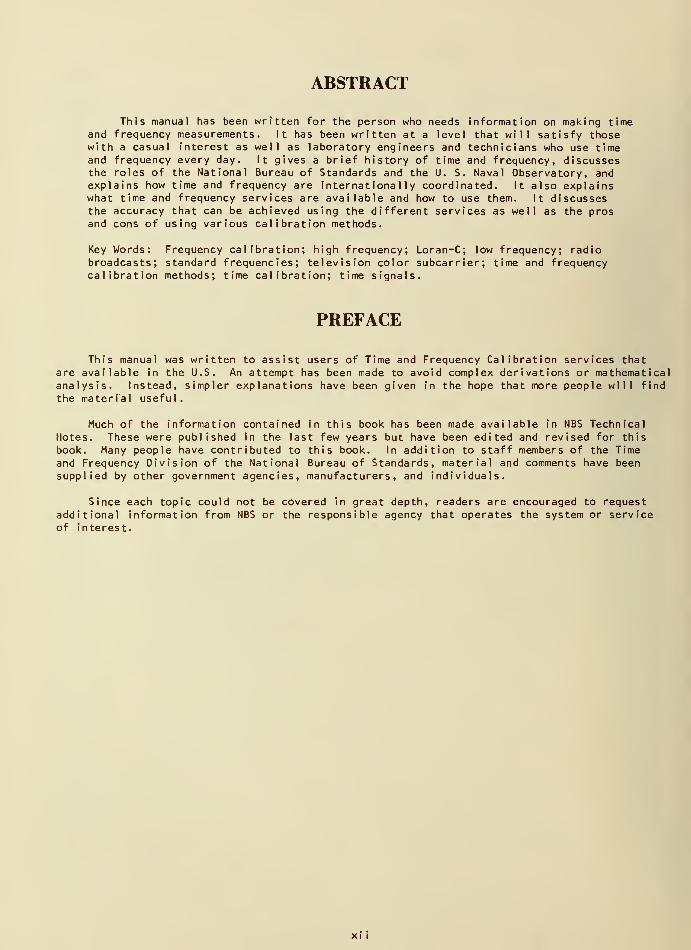
This manual has been written for the person who needs information on making timeand frequency measurements. It has been written at a level that will satisfy thosewith a casual interest as well as laboratory engineers and technicians who use timeand frequency every day. It gives a brief history of time and frequency, discussesthe roles of the National Bureau of Standards and the U. S. Naval Observatory, andexplains how time and frequency are internationally coordinated. It also explainswhat time and frequency services are available and how to use them. It discussesthe accuracy that can be achieved using the different services as well as the prosand cons of using various calibration methods.
Key Words: Frequency calibration; high frequency; Loran-C; low frequency; radiobroadcasts; standard frequencies; television color subcarrier; time and frequencycalibration methods; time calibration; time signals.
PREFACE
This manual was written to assist users of Time and Frequency Calibration services thatare available in the U.S. An attempt has been made to avoid complex derivations or mathematicalanalysis. Instead, simpler explanations have been given in the hope that more people will find
the material useful
.
Much of the information contained in this book has been made available in NBS TechnicalNotes. These were published in the last few years but have been edited and revised for thisbook. Many people have contributed to this book. In addition to staff members of the Time
and Frequency Division of the National Bureau of Standards, material and comments have been
supplied by other government agencies, manufacturers, and individuals.
Since each topic could not be covered in great depth, readers are encouraged to requestadditional information from NBS or the responsible agency that operates the system or serviceof interest.
CHAPTER 1. INTRODUCTION: WHAT THIS BOOK IS ABOUT
Time and frequency are all around us. We hear the time announced on radio and television,and we see it on the time and temperature sign at the local bank. The frequency markings onour car radio dials help us find our favorite stations. Time and frequency are so commonlyavailable that we often take them for granted; we seldom stop to think about where they comefrom or how they are measured.
Yet among the many thousands of things that man has been able to measure, time and time
interval are unique. Of all the standards
—
especially the basic standards of length, mass,
time, and temperature--time (or more properly time interval) can be measured with a greaterresolution and accuracy than any other. Even in the practical world away from the scientificlaboratory, routine time and frequency measurements are made to resolutions of parts in a
thousand billion. This is in sharp contrast to length measurements, for instance, where an
accuracy of one part in ten thousand represents a tremendous achievement.
1.1 THE DEFINITIONS OF TIME AND FREQUENCY
We should pause a moment to consider what is meant by the word "time" as we commonly use
it. Time of day or date is the most often used meaning, and even that is usually presented in
a brief form of hours, minutes, and seconds, whereas a complete statement of the time of daywould also include the day of the week, month, and year. It could also extend to units of timesmaller than the second going down through milliseconds, microseconds, nanoseconds, and picoseconds,
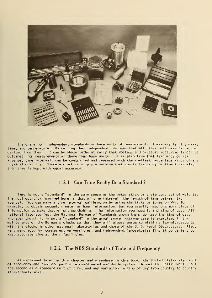
We also use the word time when we meanthe length of time between two events, calledtime intervals. The word time almost alwaysneeds additional terms to clarify its meaning;for instance, time of day or time interval .
Today time is based on the definition ofa second. A second is a time interval and it
is defined in terms of the cesium atom. Thisis explained in some detail in the chapter onatomic frequency sources. Let us say here thata second consists of counting 9.192,631,770periods of the radiation associated with thecesium-133 atom.
TIME OF DAY:
9:00 A.M.5 MINUTES
TIME INTERVAL
The definition of frequency is also based on this definition,
frequency is the hertz which is defined as one cycle per second.The term used to describe
What does all this mean to user
industrial engineer, or, for that ma
about frequency and time measurementwhat this book is about. It has bee
to set his watch and for those withoscillators or perform related scien
at a level which will satisfy all of
world today in the form of servicesIn addition to providing informationon how to use each service. Althougfrequency services, our attention in
of Standards and the U. S. Naval Obs
in Canada.
s of time and frequency? Where does the laboratory scientist,tter, the man on. the street go when he needs informations or about performing those measurements himself? That'sn written for the person with a casual interest who wantsa specific need for frequency and time services to adjusttific measurements. This book has been deliberately writtenthese users. It will explain what is available in our
that provide time and frequency for many classes of users.regarding these services, detailed explanations are given
h many countries throughout the world provide time andthis book is focused on the services of the National Bureau
ervatory in this country and the National Research Council
There are many time and frequency services. You can get time of day by listening to highfrequency radio broadcasts, or you can call the time-of-day telephone services. You can decodetime codes broadcast on various high, low, and very low frequency radio stations. You canmeasure frequency by accessing certain signals on radio and television broadcasts. You can
obtain literature explaining the various services. And if your needs are critical, you cancarry a portable clock to NBS or the USNO for comparison. All of these services are explainedin this book.
1.2 WHAT IS A STANDARD ?
Of course, before you can have a standard frequency and time service , you have to have a
standard , but what is it? The definition of a legal standard is just that--a legal definitionthat tells you where the ultimate comparison must be made. In the United States, the NationalBureau of Standards (NBS) is responsible for maintaining and disseminating standards of physicalmeasurement.
There are four independent standards or base units of measurement. These are length, mass,
time, and temperature. By calling them independent, we mean that all other measurements can be
derived from them. It can be shown mathematically that voltage and pressure measurements can be
obtained from measurements of these four base units. It is also true that frequency or its
inverse, time interval, can be controlled and measured with the smallest percentage error of anyphysical quantity. Since a clock is simply a machine that counts frequency or time intervals,
then time is kept with equal accuracy.
1.2.1 Can Time Really Be a Standard ?
Time is not a "standard" in the same sense as
The real quantity involved here is that of time in
events). You can make a time interval calibrationexample, to obtain second, minute, or hour informainformation to make that effort worthwhile. The i
national laboratories, the National Bureau of Stan
and even though it is not a "standard" in the usua
maintenance of the Bureau's clocks so that they wi
with the clocks in other national laboratories andmany manufacturing companies, universities, and in
keep accurate time at their facilities.
the meter stick or a
terval (the length ofby using the ticks o
tion, but you usuallynformation you need i
dards among them, do
I sense, extreme careII always agree to wi
those of the U. S. N
dependent laboratorie
standard set of weights.time between two
r tones on WWV, forneed one more piece of
s the time of day. Al
1
keep the time of day;
is exercised in the
thin a few microsecondsaval Observatory. Also,
s find it convenient to
1.2.2 The NBS Standards of Time and Frequency
As explained later in this chapter and elsewhere in this book, the United States standardsof frequency and time are part of a coordinated worldwide system. Almost the entire world usesthe second as a standard unit of time, and any variation in time of day from country to countryis extremely smal 1
.
But unlike the other standards, time is always changing; so can you really have a time
standard? We often hear the term standard time used in conjunction with time zones. But is
there a standard time kept by the National Bureau of Standards? Yes there is, but because of
its changing nature, it doesn't have the same properties as the other physical standards, suchas length and mass. Although NBS does operate a source of time, it is adjusted periodically to
agree with clocks in other countries. In the next chapter we will attempt to explain the basisfor making such changes and how they are managed and organized throughout the world.
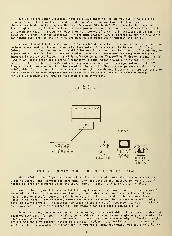
So even though NBS does not have a glass-enclosed clock that is
do have a standard for frequency and time intervals. This standard i
Colorado. It carries the designation NBS-6 because it is the sixth i
lators built and maintained by NBS to provide the official referenceinterval in the United States. NBS-6 is referred to as the "master"used to calibrate other oscillators ("secondary" clocks) which are us
scale. (A time scale is a system of counting pendulum swings.) Thefrequency and time standard is illustrated in figure 1.1. Shown is t
NBS-6, which is used to calibrate an ensemble of other atomic oscillascale, which is in turn compared and adjusted to similar time scalesPeriodic adjustments are made to keep them all in agreement.
untouched or unadjusted, wes located in Boulder,n a series of atomic oscil-for frequency and timeor "primary" clock. It is
ed to operate the timeorganization of the NBS
he primary atomic standardtors which operate the timein other countries.
NBS-6(PRIMARY CLOCK)
(SECONDARY CLOCKS)
TIMESCALE
SERVICES
COMPARISONSWITH TIMESCALES IN
OTHER COUNTRIES
ElRADIO
JROADCASTS
TELEVISION / *-
TIME & %/TESRFREQUENCY '{_ JTRANSFER TELEPHONE
TIME-OF-DAYSERVICE
FIGURE 1.1. ORGANIZATION OF THE NBS FREQUENCY AND TIME STANDARD.
The useful output of the NBS standard and its associated time scale are the services pro-
vided to users. This service can take many forms and uses several methods to get the actual
needed calibration information to the user. This, in part, is what this book is about.
Notice that figure 1.1 looks a lot like any timepiece. We have a source of frequency, a
means of counting that frequency and keeping time of day in a time scale, and as mentioned, a
way of getting a useful output. This is exactly what is contained in almost every clock or
watch in use today. The frequency source can be a 60 Hz power line, a balance wheel, tuning
fork, or quartz crytal. The counter for totaling the cycles of frequency into seconds, minutes,
and hours can be gears or electronics. The readout can be a face clock or digits.
In early times, the sun was the only timekeeping device available. It had certain disadvan-
tages—cloudy days, for one. And also, you could not measure the sun angle very accurately. So
people started developing clocks so they could have time indoors and at night. Surely , though,
the sun was their "standard" instead of a clock. Outdoors, the sundial was their counter and
readout. It is reasonable to suppose that if you had a large hour glass, you could hold it next
to the sundial and write the hour on it, turn it over, and then transport it indoors to keep
the time fairly accurately for the next hour. A similar situation exists today in that secondary
clocks are brought to the master or primary clock for accurate setting and then used to keep
time.
1.3 HOW TIME AND FREQUENCY STANDARDS ARE DISTRIBUTED
In addition to generating and distributing standard frequency and time interval, the
National Bureau of Standards also broadcasts time of day via its radio stations WWV and WWVH.Each of the fifty United States has a state standards laboratory which deals in many kinds of
standards, including those of frequency and time interval. Few of these state labs get involvedwith time of day, which is usually left to the individual user, but many of them can calibratefrequency sources that are used to check timers such as those used in automatic washers, carwashes, and parking meters.
In private industry and other government agencies where standards labs are maintained, a
considerable amount of time and frequency work is performed, depending on the end product ofthe company. As you might guess, electronics manufacturers who deal with counters, oscillators,and signal generators are very interested in having an available source of accurate frequency.This will very often take the form of an atomic oscillator kept in the company's standards lab
and calibrated against NBS.
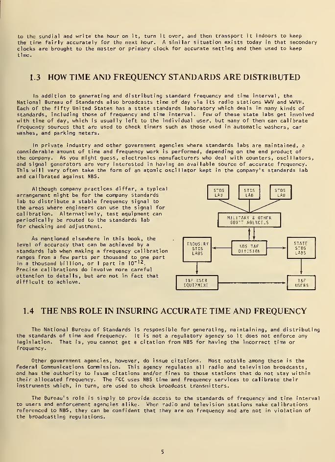
Although company practices differ, a typical
arrangement might be for the company standardslab to distribute a stable frequency signal to
the areas where engineers can use the signal for
calibration. Alternatively, test equipment can
periodically be routed to the standards lab
for checking and adjustment.
As mentioned elsewhere in this book, thelevel of accuracy that can be achieved by a
standards lab when making a frequency calibrationranges from a few parts per thousand to one partin a thousand billion, or 1 part in 10~'2.
Precise calibrations do involve more carefulattention to details, but are not in fact thatdifficult to achieve.
1 .4 THE NBS ROLE IN INSURING ACCURATE TIME AND FREQUENCY
The National Bureau of Standards is responsible for generating, maintaining, and distributingthe standards of time and frequency. It is not a regulatory agency so it does not enforce anylegislation. That is, you cannot get a citation from NBS for having the incorrect time orfrequency.
Other government agencies, however, do issue citations. Most notable among these is the
Federal Communications Commission. This agency regulates all radio and television broadcasts,and has the authority to issue citations and/or fines to those stations that do not stay withintheir allocated frequency. The FCC uses NBS time and frequency services to calibrate theirinstruments which, in turn, are used to check broadcast transmitters.
The Bureau's role is simply to provide access to the standards of frequency and time intervalto users and enforcement agencies alike. When radio and television stations make calibrationsreferenced to NBS, they can be confident that they are on frequency and are not in violation ofthe broadcasting regulations.
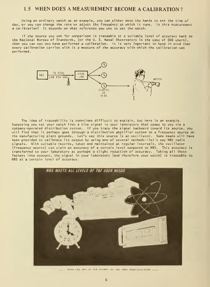
1.5 WHEN DOES A MEASUREMENT BECOME A CALIBRATION ?
Using an ordinary watch as an example, you can either move the hands to set the time ofday, or you can change the rate or adjust the frequency at which it runs. Is this measurementa calibration? It depends on what reference you use to set the watch.
If the source you use for comparison is traceable at a suitable level of accuracy back to
the National Bureau of Standards, (or the U. S. Naval Observatory in the case of DOD users),then you can say you have performed a calibration. It is very important to keep in mind thatevery calibration carries with it a measure of the accuracy with which the calibration wasperformed.
WATCH
The idea of traceability is somet
Supposing you set your watch from a ti
company-operated distribution system,will find that it perhaps goes throughthe manufacturing plant grounds. Let 1
been provided to calibrate its outputsignals. With suitable records, taken
(frequency source) can claim an accuratransferred to your laboratory at perh
factors into account, the signal in yoNBS at a certain level of accuracy.
imes difficult to explain, but here is an example,me signal in your laboratory that comes to you via a
If you trace the signal backward toward its source, youa distribution amplifier system to a frequency source on
s say this source is an oscillator. Some means will have
by using one of several methods--let ' s say NBS radioand maintained at regular intervals, the oscillator
cy of a certain level compared to NBS. This accuracy is
aps a slight reduction of accuracy. Taking all these
ur laboratory (and therefore your watch) is traceable to
from the man on the street to the very sophisticated
What kind of accuracy is obtainable? As we said before, frequency and time can both bemeasured to very high accuracies with very great measurement resolution. As this book explains,there are many techniques available to perform calibrations. Your accuracy depends on whichtechnique you choose and what errors you make in your measurements. Typically, frequencycalibration accuracies range from parts per million by high frequency radio signals to parts perhundred billion for television or Loran-C methods. A great deal depends or. how much effort youare willing to expend to get a good, accurate measurement.
1.6 TERMS USED
1 .6. 1 Mega, MLli, Parts Per . . . and Percents
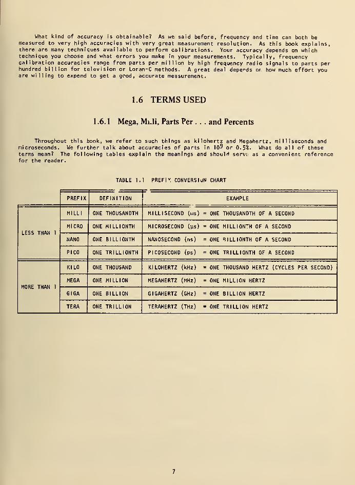
Throughout this book, we refer to such things as kllohertz and Megahertz, milliseconds andmicroseconds. We further talk about accuracies of parts in I()9 or 0.51. What do all of theseterms mean? The following tables explain the meanings and shoulH serve: as a convenient referencefor the reader.
TABLE 1.1 PREFI V CONVERSION CHART
PREFIX DEFINITION EXAMPLE
LESS THAN 1
MILLI ONE THOUSANDTH MILLISECOND (ms) = ONE THOUSANDTH OF A SECOND
MICRO ONE MILLIONTH MICROSECOND (ys) = ONE MILLIONTH OF A SECOND
NANO ONE BILLIONTH NANOSECOND (ns) - ONE BILLIONTH OF A SECOND
PICO ONE TRILLIONTH PICOSECOND (ps) = ONE TRILLIONTH OF A SECOND
MORE THAN 1
KILO ONE THOUSAND KILOHERTZ (kHz) = ONE THOUSAND HERTZ (CYCLES PER SECOND)
MEGA ONE MILLION MEGAHERTZ (MHz) = ONE MILLION HERTZ
GIGA ONE BILLION GIGAHERTZ (GHz) = ONE BILLION HERTZ
TERA ONE TRILLION TERAHERTZ (THz) = ONE TRILLION HERTZ
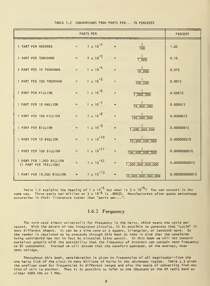
TABLE 1.2 CONVERSIONS FROM PARTS PER... TO PERCENTS
PARTS PER PERCENT
1 PART PER HUNDRED
1 PART PER THOUSAND
1 PART PER 10 THOUSAND
1 PART PER 100 THOUSAND
1 PART PER MILLION
1 PART PER 10 MILLION
1 PART PER 100 MILLION
1 PART PER BILLION
1 PART PER 10 BILLION
1 PART PER 100 BILLION
1 PART PER 1 ,000 BILLION
(1 PART PER TRILLION)
1 PART PER 10,000 BILLION
1 x 10
1 x 10⁻³
1 x 10
1 x 10
1 x 10
1 x 10
1 x 10
-k
1 x 10
1 x 10
1 x 10
-9
10
11
1 x 10-12
1 x 10-13
1
100
1
1 ,000
1
10,000
1
100,000
1
1,000,000
1
10,000,000
1
100,000,000
1
1 ,000,000,000
1
10,000,000,000
1
100,000,000,000
1
1 ,000,000,000,000
1
10,000,000,000,000
1.0%
0.1%
o.oi%
0.001%
0.0001%
0.00001%
0.000001%
0.0000001%
0.00000001%
0.000000001%
0.0000000001%
0.00000000001%
Table 1.2 explains the meaning of 1 x 10 but what is 3 x 10 ? You can convert in the
same way. Three parts per million or 3 x 10"" is .0003%. Manufacturers often quote percentageaccuracies in their literature rather than "parts per...".
1.6.2 Frequency
The term used almost universally for frequency is the hertz, which means one cycle per
second. With the advent of new integrated circuits, it is possible to generate that "cycle" in
many different shapes. It can be a sine wave or a square, triangular, or sawtooth wave. So
the reader is cautioned as he proceeds through this book to keep in mind that the waveformsbeing considered may not in fact be sinusoids (sine waves). In this book we will not concern
ourselves greatly with the possibility that the frequency of interest can contain zero frequency
or DC components. Instead we will assume that the waveform operates, on the average, near
zero voltage.
Throughout this book, consideration is given to frequencies of all magnitudes—from the
one hertz tick of the clock to many billions of hertz in the microwave region. Table 1.3 gives
the prefixes used for frequencies in different ranges and also the means of converting from one
kind of unit to another. Thus it is possible to refer to one thousand on the AM radio band as
either 1000 kHz or 1 MHz.
8
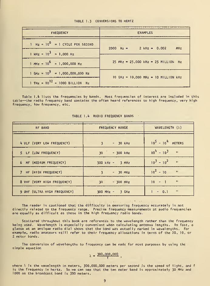
TABLE 1.3 CONVERSIONS TO HERTZ
FREQUENCY EXAMPLES
1 Hz = 10° =1 CYCLE PER SECOND2000 Hz = 2 kHz = 0.002 MHz
1 kHz = 103 = 1,000 Hz
25 MHz = 25,000 kHz = 25 MILLION Hz1 MHz = 10
6= 1,000,000 Hz
1 GHz = 109 = 1,000,000,000 Hz
10 GHz = 10,000 MHz = 10 MILLION kHz
1 THz = 1012
= 1000 BILLION Hz
Table 1 .4 lists the frequencies by bands. Most frequencies of interest are included in this
table--the radio frequency band contains the often heard references to high frequency, very high
frequency, low frequency, etc.
TABLE 1.4 RADIO FREQUENCY BANDS
RF BAND FREQUENCY RANGE WAVELENGTH (X)
h VLF (VERY LOW FREQUENCY) 3 - 30 kHz 105
- 10^ METERS
5 LF (LOW FREQUENCY) 30 - 300 kHzk 3
10 - 1015
6 MF (MEDIUM FREQUENCY) 300 kHz - 3 MHz 103
- io2
7 HF (HIGH FREQUENCY) 3 - 30 MHz 102
- 10
8 VHF (VERY HIGH FREQUENCY) 30 - 300 MHz 10-1 "
9 UHF (ULTRA HIGH FREQUENCY) 300 MHz - 3 GHz 1 - 0.1
The reader is cautioned that the difficulty in measuring frequency accurately is not
directly related to the frequency range. Precise frequency measurements at audio frequenciesare equally as difficult as those in the high frequency radio bands.
Scattered throughout this book are references to the wavelength rather than the frequencybeing used. Wavelength is especially convenient when calculating antenna lengths. In fact, a
glance at an antique radio dial shows that the band was actually marked in wavelengths. For
example, radio amateurs still refer to their frequency allocations in terms of the 20, 10, or2 meter bands.
The conversion of wavelengths to frequency can be made for most purposes by using thesimple equation
\ = 300,000,000
where A. is the wavelength in meters, 300,000,000 meters per second is the speed of light, and f
is the frequency in hertz. So we can see that the ten meter band is approximately 30 MHz and1000 on the broadcast band is 300 meters.
The above equation can be converted to feet and inches for ease in cutting antennas toexact length. Precise calculations of wavelength would have to take into account the mediumand allow for the reduced velocity below that of light, for instance, inside coaxial cables.
Many users of frequency generating devices tend to take frequency for granted, especiallyin the case of crystals. A popular feeling is that if the frequency of interest has beengenerated from a quartz crystal, it cannot be in error by any significant amount. This is
simply not true. Age affects the frequency of all quartz oscillators. Although frequency canbe measured more precisely than most phenomena, it is still the responsibility of the calibrationlaboratory technician or general user to keep in mind the tolerances needed; for example,musical notes are usually measured to a tenth of a hertz or better. Power line frequency is
controlled to a millihertz. If you dial the NBS time-of-day telephone service, you will hearaudio frequency tones that, although generated to an accuracy of parts per 10^, can be sentover the telephone lines only to a few parts In one thousand. So the responsibility is theusers t<" decide what he needs and whether, in fact, the measurement scheme he chooses willsatisfy .lose needs.
Throughout this book, mention is made of the ease with which frequency standards can becalibrated to high precision. Let us assume that you have, in fact, just calibrated your highquality crystal oscillator and set the associated clock right on time. What happens next?Probably nothing happens. The oscillators manufactured today are of excellent quality and,assuming that a suitable battery supply is available to prevent power outages, the clock couldkeep very accurate time for many weeks. The kicker in this statement is, of course, the word"accurate." If you want to maintain time with an error as small or smaller than a microsecond,your clock could very easily have that amount of error in a few minutes. If you are less con-cerned with microseconds and are worried about only milliseconds or greater, a month couldelapse before such an error would reveal itself.
The point to be made here is that nothing can be taken for granted. If you come into yourlaboratory on Monday morning hoping that everything stayed put over the weekend, you might beunpleasantly surprised. Digital dividers used to drive electronic clocks do jump occasionally,especially if the power supplies are not designed to avoid some of the glitches that can occur.It makes sense, therefore, to check both time and frequency periodically to insure that thefrequency rate is right and the clock is on time.
Many users who depend heavily on their frequency source for calibrations— for example,manufacturing plants--find it convenient to maintain a continuous record of the frequency oftheir oscillators. This usually takes the form of a chart recording that shows the frequencyvariations in their oscillator versus a received signal from either a National Bureau of Standardsstation or one of the many other transmissions which have been stabilized. Among these are the
Omega and Loran-C navigation signals.
If you refer to Chapter 10 of this book, which deals with the characteristics of oscillators,you will notice that crystal oscillators and even rubidium oscillators will drift in frequencyso, depending on your application, periodic adjustments are required.
1.7 DISTRIBUTING TIME AND FREQUENCY SIGNALSVIA CABLES AND TELEPHONE LINKS
Users of time and frequency signals sometimes want to distribute either a standard
frequency waveform or a time signal using cables. This is often the case in a laboratory or
manufacturing plant where the standards laboratory provides signals for users throughout the
plant area. Of course, the solution to any given problem depends on good engineering practice
and consideration for the kind of result desired. That is to say, if you start with a cesium
oscillator and want to maintain its accuracy throughout a large area, you must use the very best
of equipment and cables; and even then, the signal accuracy will be somewhat deteriorated. On
the other hand, if all that is needed is a time-of-day signal on the company telephone switch-
board, the specifications can be relaxed.
Without knowing the particular conditions under which signals are to be distributed, it
would be hard to specify the maximum accuracy obtainable. A number of articles have been
published for distribution systems using both coaxial cables and telephone lines. The results
that the individual writers reported varied from parts per million to almost one part in 10
billion. In each case the results were in direct ratio to the amount of effort expended.
10
Since the articles were written a number of years ago, it is expected that better results could
be achieved today. Other than the good engineering practices mentioned above, there is no
simple formula for successful transmission of standard frequency and time signals.
Often the main problem is noise pickup in the cables that causes the signal at the end ofthe line to be less useful than desired. Another problem often reported is the difficulty in
certifying the received accuracy or to establish NBS traceability over such a distributionsystem. A suggestion would be that careful system management be observed and that periodicevaluation of the system be attempted. One method of evaluating a distribution system would be
to route the signal on a continuous loop and look at the signal going in and the signal comingout for a particular cable routing.
For commercial telephone lines (which are usually balanced systems), the highest practicalfrequency that can be distributed is 1000 Hz. Coaxial cables have been used successfully for
frequencies up to 100,000 Hz. Any attempt to send pulses over a voice-grade telephone line
would be unsuccessful due to the limited bandwidth.
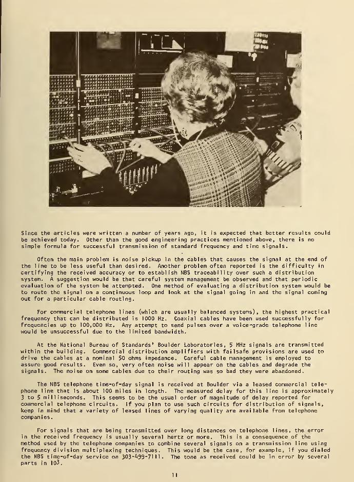
At the National Bureau of Standards' Boulder Laboratories, 5 MHz signals are transmittedwithin the building. Commercial distribution amplifiers with failsafe provisions are used to
drive the cables at a nominal 50 ohms impedance. Careful cable management is employed to
assure good results. Even so, very often noise will appear on the cables and degrade thesignals. The noise on some cables due to their routing was so bad they were abandoned.
The NBS telephone time-of-day signal is received at Boulder via a leased commercial tele-phone line that is about 100 miles in length. The measured delay for this line is approximately3 to 5 milliseconds. This seems to be the usual order of magnitude of delay reported for
commercial telephone circuits. If you plan to use such circuits for distribution of signals,keep in mind that a variety of leased lines of varying quality are available from telephonecompanies
.
For signals that are being transmitted over long distances on telephone lines, the errorin the received frequency is usually several hertz or more. This is a consequence of the
method used by the telephone companies to combine several signals on a transmission line usingfrequency division multiplexing techniques. This would be the case, for example, if you dialedthe NBS time-of-day service on 303-^99-7111- The tone as received could be in error by severalparts in 103.
11
For those users wanting to distribute either very accurate frequency or precise time, i
is almost fair to say that local cable and wire systems are not economically practical. If
your requirements are critical, it is usually cheaper in the long run to simply reestablishtime and/or frequency at the destination point. The burden of installing and maintaining a
distribution system can be very great for high accuracy systems.
1.8 TIME CODES
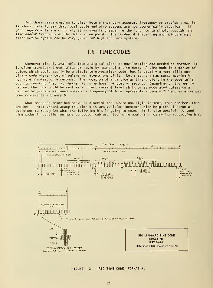
Whenever time is available from a digital clock at one location and needed at another, it
is often transferred over wires or radio by means of a time code. A time code is a series ofpulses which could easily be a simple teletypewriter code, but is usually a more efficientbinary code where a set of pulses represents one digit. Let's say a k was sent, meaning k
hours, h minutes, or h seconds. The location of a particular binary digit in the code tellsyou its meaning; that is, whether it is an hour, minute, or second. Depending on the appli-cation, the code could be sent as a direct current level shift or as modulated pulses on a
carrier or perhaps as tones where one frequency of tone represents a binary "1" and an alternatetone represents a binary 0.
What has been described above is a serial code where one digit is sent, then another, then
another. Interspersed among the time bits are position locators which help the electronicequipment to recognize what the following bit is going to mean. It is also possible to send
time codes in parallel on many conductor cables. Each wire would then carry its respective bit.
TIME FRAME 1 MINUTE20 30 40 50
i i i i|
i i '[' t l l l|
I I I I|
I I I' |
I'
I I I ' ' 'I
|I
' ' ' | ' ' ' ' I ' ' '
REFERENCE TIME INDEX COUNT I SEC.
-REFERENCE MARK ER
UU1 IU lUUU1 2 4 S 10 20 40 1 2 4 B 10 20 40 80 100 200
LHULMJlimJLJTJlJULJLJL^^— 0.2 SEC.BINARYITYPICAL) — 0.5 SEC.
BINARY '!'
ITYPICAL)
P4- 1 SEC.(TYPICAL)
0.8 SEC.POSITIONIDENTIFIER(TYPICAL)
lh,s po.nl equols 173 days, 21 hours, 24 m.nules, 57 seconds
TYPICAL MODULATED CARRIER
Recommended Frequency 100 Hi or 1000 Hz
IRIG STANDARD TIME CODEFORMAT H'
(IPPSCode)
Reference IRIG Document 104-70
FIGURE 1.2. IRIG TIME CODE, FORMAT H,
12
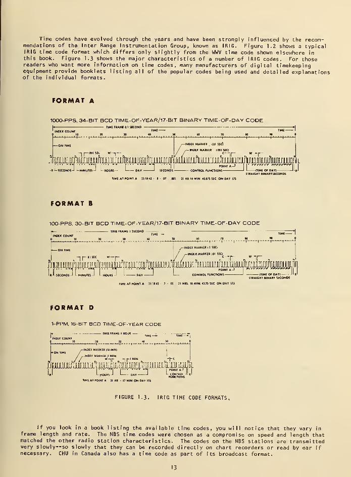
Time codes have evolved through the years and have been strongly influenced by the recom-mendations of the Inter Range Instrumentation Group, known as IRIG. Figure 1.2 shows a typicalIRIG time code format which differs only slightly from the WWV time code shown elsewhere in
this book. Figure 1.3 shows the major characteristics of a number of IRIG codes. For thosereaders who want more information on time codes, many manufacturers of digital timekeepingequipment provide booklets listing all of the popular codes being used and detailed explanationsof the individual formats.
FORMAT A
10O0-PPS, 34-BIT BCD TIME-OF-YEAR/17-BIT BINARY TIME-OF-DAY CODE
INDEX COUIfl10
I' ' '
I
'
TIME FUME 0.1 SECOND
30-*--
I' '
'' I
' ' ' ' t-*-1-
TIMi
401
I' ' ' '
I' '
'
,ir 001 SEC W~ir,
[ "If ][_"" "1 ill 1 r "!
t"- SECONDS^ L_ MINUTES -> L HOURS —' I DAT * SECOND
FORMAT B
i ' ' i
'
•+1
TIME-
MII
'"
I'
-INDEX MARKED 101 SEcl
INDEX MARKER 1001 SECI
JilMiJlllijtL_j II' jTiTi«i*?i'i« i^"i"i"ii »i,'i«t» 1
1
POINT A- CONTROL FUNCTIONS -(TIME OF DAY)-
STRAICHT BINARY SECONDS
TIME AT POINT A 31 1842 S 07 005 21 HR 18 MIN 42875 SEC ON DAY 173
100-PPS. 30-BIT BCD TIME-OF-YEAR/17-BIT BINARY TIME-OF-DAY CODE|a_ TIME FRAME I SECOND —' IMP1 INDEX COUNT
I' ' ' '
I
'—'T ' ' ' '
I' ' ' '
I' ' ' '
I' ' ' '
I' ' ' '
I' ' ' '
I'
"'
INDEX MARKER II SEC)
INDEX MARKER 101 SEC)/ ,— inucx m*»*ncw |.ui Jtv.i
I
—^ p- oi stc w^|p V /c^ir~
wnrmjiiiMJ'jwi^
'
I
I hi "I I"" ] i
"1 poin,aJI r
I-R-LSECONDSJ L MINUIesJ L HOURS J I DAY ' CONTROL FUNCTIONS
jijt ri*T*1'i* *rtnjawwrt
(TIME OF DAY) '
STRAIGHT BINARY SECONDS
TIME AT POINT A 21 18:42 7 OS 21 HRS 18 MIN 42 7S SEC ON DAY 173
FORMAT D
1-PPM. 16-BIT BCD TIME-OF-YEAR CODEU- - TIME FRAME 1 HOUR - - - -
1 INDEX COUNT30
-INDEX MARKER (10 MIN)
-INDEX MARKER (I MIN)
r/ wir ir' MiN ,hh c
I'1 {••' >»"« —
I
I POINT A JTl
LuoURsJ ' DAY 1L CON1ROI-flOURS-1 I OAY -
TIME AT POINT A 31 HR. . S7 MIN ON DAY 17}
FIGURE 1,3. IRtG TIME CODE FORMATS.
If you look in a book listing the available time codes, you will notice that they vary inframe length and rate. The NBS time codes were chosen as a compromise on speed and length thatmatched the other radio station characteristics. The codes on the NBS stations are transmittedvery slowly—so slowly that they can be recorded directly on chart recorders or read by ear ifnecessary. CHU in Canada also has a time code as part of its broadcast format.
13
The time codes provided on the National Bureau of Standards' radio stations WWV, WWVH , andWWVB can be used for clock setting. But because of fading and noise on the radio path, thesepulses cannot usually be used directly for operating a time display. Instead, the informationis received and decoded and used to reset a clock that is already operating and keeping time.However, the noise and fading often cause errors in' the decoding so any clock system thatintends to use radio time codes must have provisions to flywheel with a crystal oscillator andmaintain the required accuracy between the successful decodes.
Does this mean that the time codes as transmitted and received are of little practicalvalue? No, on the contrary. There are so few sources of accurate, distributed time that thesetime codes are of immense value to people who must keep time at remote locations. The descrip-tion of how to use the time codes would suggest that they are complicated and cumbersome. Thismay have been true a few years ago. But with the advent of modern integrated circuit technology,both the cost and complexity have been reduced to manageable proportions. The real point to benoticed is that the code cannot be used directly but must be used to reset a running clock withsuitable data rejection criteria.
As of this writing (1977), information obtained by the National Bureau of Standards fromits mail and direct contact with users suggests that time codes will be used more and more.Several factors have strongly influenced this increased usage. One of these is the availabilityof low-cost digital clocks. The other factor, as previously mentioned, seems to be the costreductions in integrated circuits. These circuits are so inexpensive and dependable that theyhave made possible new applications for time codes that were impractical with vacuum tubes.
The accuracy of time codes as received depends on a number of factors. First of all, youhave to account for the propagation path delay. A user who is 1000 miles from the transmitterexperiences a delay of about 5 microseconds per mile. This works out to be 5 milliseconds timeerror. To this we must add the delay through the receiver. The signal does not instantly gofrom the receiving antenna to the loudspeaker or the lighted digit. A typical receiver delaymight be one-half millisecond. So a user can experience a total delay as large as 8 to 10
milliseconds, depending on his location. This amount of delay is insignificant for most users.
But for those few who do require accurate synchronization or time of day, there is a method for
removing the path delay. Manufacturers of time code receivers very often include a simpleswitching arrangement to dial out the path delay. When operating time code generators, the
usual recommendations for battery backup should be followed to avoid errors in the generatedcode.
THE UTILITY OF TIME CODES . In addition to using codes for setting remote clocks from,say, a master clock, time codes are used on magnetic tape systems to search for information.
The time code is recorded on a separate tape track. Later, the operator can locate and identifyinformation by the time code reading associated with that particular spot on the tape. Manymanufacturers provide time code generation equipment expressly for the purpose of tape search.
Another application of time codes is for identifying events. The Federal AviationAdministration records the WWV time code on its audio tapes on which are also recorded the air-to-ground communications from airplanes. In this way, it is possible to go back and reconstructconversations and use the time code for determining when a particular event happened. For
example, this information could be an important factor in determining the cause of a planecrash.
There are many other uses. The electric power industry automatically receives the time code
from WWVB, decodes the time of day, and uses this information to steer the electric powernetwork. Many of the telephone companies use a decoded signal to drive their machines whichactually answer the phone when you dial the time of day. Even bank signs that give time and
temperature are often driven from the received time code. Why is this? The main reason a time
code is used is to avoid errors. It also reduces the amount of work that must be done to keep
the particular clock accurate.
14
CHAPTER 2. THE EVOLUTION OF TIMEKEEPING
2.1 TIME SCALES
A time scale is simply a system of assigning dates to events or counting pendulum swings.The apparent motion of the sun in the sky is one type of time scale, called astronomical time.Today, we also have atomic time, where an atomic oscillator is the "pendulum". To see how thevarious time scales came about, let's take a brief look at the evolution of time.
2.1.1 Solar Time
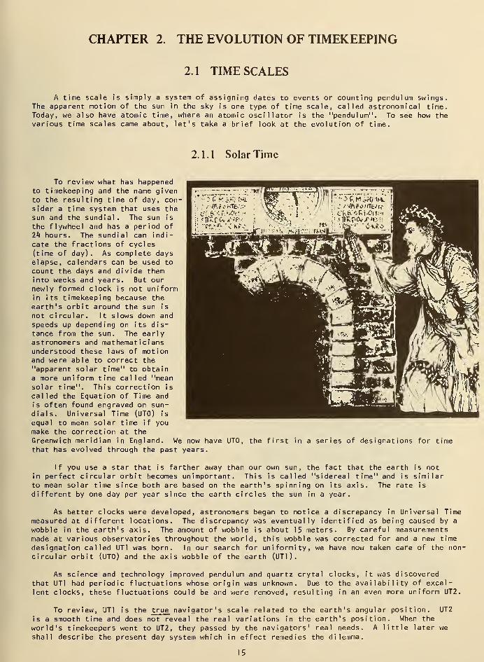
To review what has happenedto timekeeping and the name givento the resulting time of day, con-
sider a time system that uses thesun and the sundial. The sun is
the flywheel and has a period of
2k hours. The sundial can indi-
cate the fractions of cycles(time of day). As complete dayselapse, calendars can be used to
count the days and divide theminto weeks and years. But ournewly formed clock is not uniformin its timekeeping because the
earth's orbit around the sun is
not circular. It slows down and
speeds up depending on its dis-tance from the sun. The earlyastronomers and mathematiciansunderstood these laws of motionand were able to correct the
"apparent solar time" to obtaina more uniform time called "meansolar time". This correction is
called the Equation of Time and
is often found engraved on sun-dials. Universal Time (UTO) is
equal to mean solar time if youmake the correction at theGreenwich meridian in England. We now have UTO, the first in a series of designations for timethat has evolved through the past years.
If you use a star that is farther away than our own sun, the fact that the earth is notin perfect circular orbit becomes unimportant. This is called "sidereal time" and is similarto mean solar time since both are based on the earth's spinning on its axis. The rate is
different by one day per year since the earth circles the sun in a year.
As better clocks were developed, astronomers began to notice a discrepancy in Universal Timemeasured at different locations. The discrepancy was eventually identified as being caused by a
wobble in the earth's axis. The amount of wobble is about 15 meters. By careful measurementsmade at various observatories throughout the world, this wobble was corrected for and a new time
designation called UT1 was born. In our search for uniformity, we have now taken care of the non-
circular orbit (UTO) and the axis wobble of the earth (UT1).
As science and technology improved pendulum and quartz crytal clocks, it was discoveredthat UT1 had periodic fluctuations whose origin was unknown. Due to the availability of excel-lent clocks, these fluctuations could be and were removed, resulting in an even more uniform UT2
.
To review, UT1 is the true navigator's scale related to the earth's angular position. UT2
is a smooth time and does not reveal the real variations in the earth's position. When the
world's timekeepers went to UT2, they passed by the navigators' real needs. A little later we
shall describe the present day system which in effect remedies the dilemma.
15
Up until now we have been talking aboutthe Universal Time family, and figure 2.1 showsthe relationship between the different universaltimes. Let us now examine the other members of
the time family. The first of these is "ephem-eris time". An ephemeris is simply a table that
predicts the positions of the sun, moon, and
planets. It was soon noticed that these pre-
dicted positions on the table did not agreewith the observed position. An analysis of
the difficulty showed that in fact the rota-
tional rate of the earth was not a constant,and this was later confirmed with crystal andatomic clocks. In response to this problem,the astronomers created what is called "ephem-eris time". It is determined by the orbit of
the earth about the sun, not by the rotationof the earth on its axis.
UNIVERSAL TIME FAMILY
APPARENT SOLAR TIME
CORRECTED BY
EQUATION OF TIME | MEAN SOLAR TIMET[0T0)
CORRECTED FOR
MIGRATION OF POLES
At -0.05sec | UT1
CORRECTED FOR
KNOWN PERIODICITY
At ~ 05sec } UT2
FIGURE 2. UNIVERSAL TIME FAMILY RELATIONSHIPS.
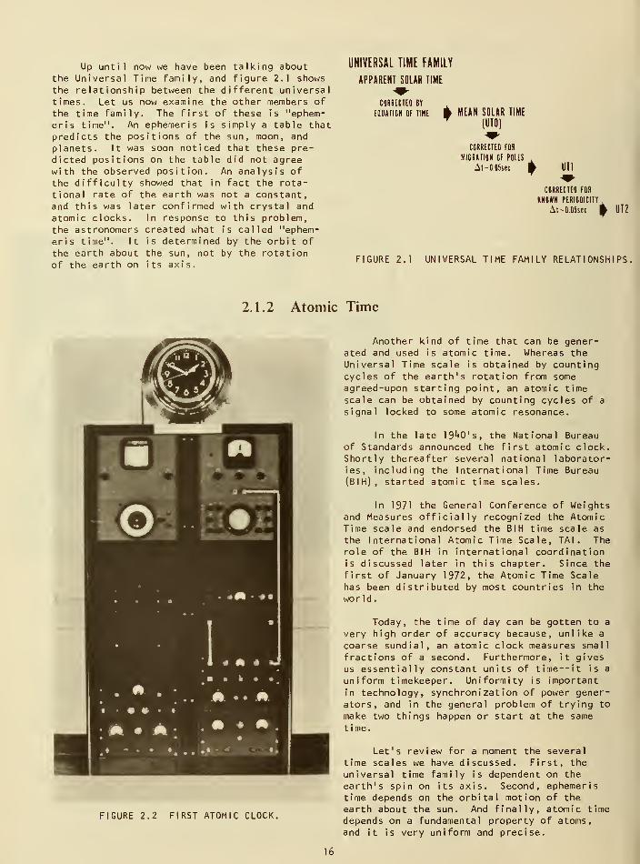
2.1.2 Atomic Time
FIGURE 2.2 FIRST ATOMIC CLOCK.
Another kind of time that can be gener-ated and used is atomic time. Whereas the
Universal Time scale is obtained by countingcycles of the earth's rotation from someagreed-upon starting point, an atomic timescale can be obtained by counting cycles of a
signal locked to some atomic resonance.
In the late 19^0
' s , the National Bureauof Standards announced the first atomic clock.Shortly thereafter several national laborator-ies, including the International Time Bureau(BIH), started atomic time scales.
In 1971 the General Conference of Weightsand Measures officially recognized the AtomicTime scale and endorsed the BIH time scale as
the International Atomic Time Scale, TAI. Therole of the BIH in international coordinationis discussed later in this chapter. Since the
first of January 1972, the Atomic Time Scalehas been distributed by most countries in the
world
.
Today, the time of day can be gotten to a
very high order of accuracy because, unlike a
coarse sundial, an atomic clock measures small
fractions of a second. Furthermore, it givesus essentially constant units of time--it is a
uniform timekeeper. Uniformity is important
in technology, synchronization of power gener-ators, and in the general problem of trying to
make two things happen or start at the same
time.
Let's review for a moment the several
time scales we have discussed. First, the
universal time family is dependent on the
earth's spin on its axis. Second, ephemeristime depends on the orbital motion of the
earth about the sun. And finally, atomic timedepends on a fundamental property of atoms,and it is very uniform and precise.
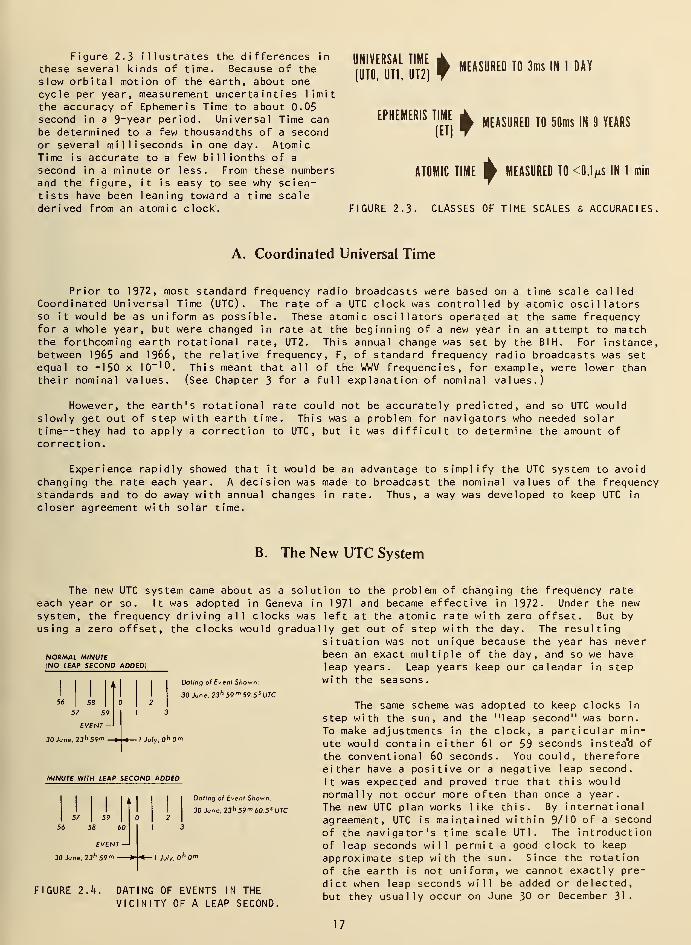
Figure 2.3 illustrates the differences in
these several kinds of time. Because of the
slow orbital motion of the earth, about onecycle per year, measurement uncertainties limitthe accuracy of Ephemeris Time to about 0.05second in a 9~year period. Universal Time canbe determined to a few thousandths of a secondor several milliseconds in one day. AtomicTime is accurate to a few billionths of a
second in a minute or less. From these numbersand the figure, it is easy to see why scien-tists have been leaning toward a time scalederived from an atomic clock.
UNIVERSAL TIME
[UTO, UN, UT2)t MEASURED TO 3ms IN 1 DAY
t MEASURED TO 50ms IN 9 YEARS
ATOMIC TIME ^ MEASURED TO 0.1/*s IN 1 min
FIGURE 2.3. CLASSES OF TIME SCALES S ACCURACIES.
EPHEMERIS TIME
(ET)
A. Coordinated Universal Time
Prior to 1972, most standard frequency radio broadcasts were based on a time scale calledCoordinated Universal Time (UTC) . The rate of a UTC clock was controlled by atomic oscillatorsso it would be as uniform as possible. These atomic oscillators operated at the same frequencyfor a whole year, but were changed in rate at the beginning of a new year in an attempt to matchthe forthcoming earth rotational rate, UT2. This annual change was set by the BIH. For instance,between 1965 and 1966, the relative frequency, F, of standard frequency radio broadcasts was setequal to -150 x 10~'0. This meant that all of the WWV frequencies, for example, were lower thantheir nominal values. (See Chapter 3 for a full explanation of nominal values.)
However, the earth's rotational rate could not be accurately predicted, and so UTC wouldslowly get out of step with earth time. This was a problem for navigators who needed solartime--they had to apply a correction to UTC, but it was difficult to determine the amount ofcorrection.
Experience rapidly showed that it would be an advantage to simplify the UTC system to avoidchanging the rate each year. A decision was made to broadcast the nominal values of the frequencystandards and to do away with annual changes in rate. Thus, a way was developed to keep UTC in
closer agreement with solar time.
B. The New UTC System
The new UTC system came about as a solueach year or so. It was adopted in Geneva i
system, the frequency driving all clocks wasusing a zero offset, the clocks would gradua
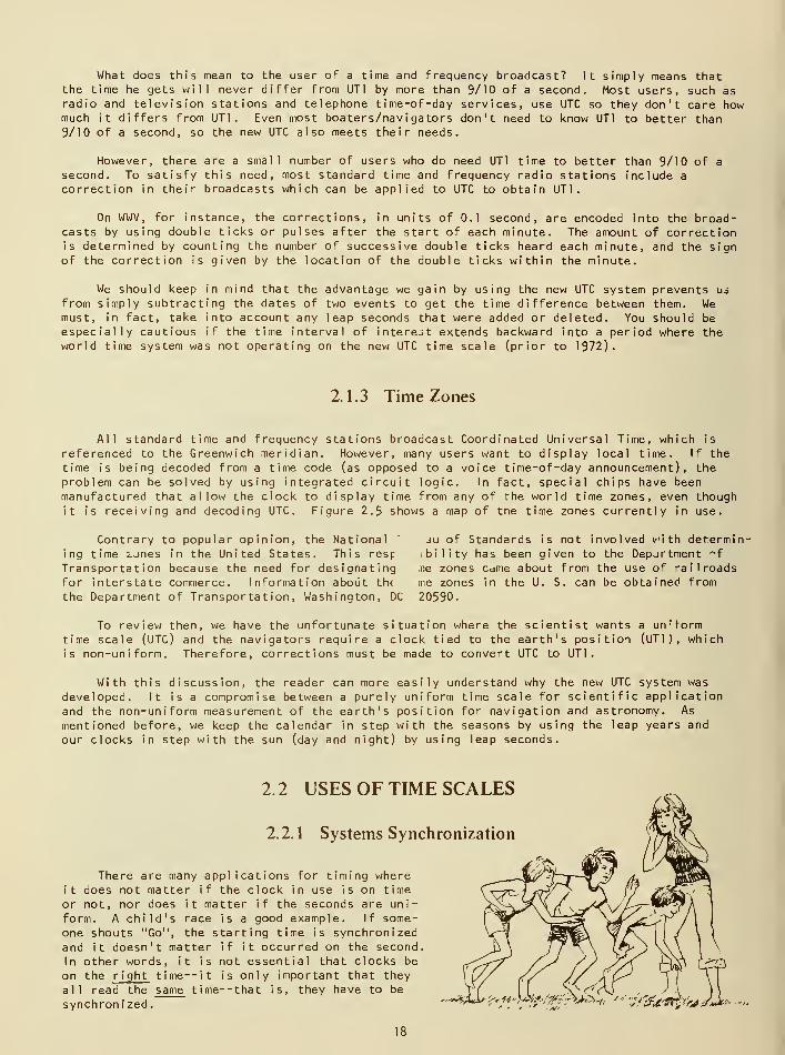
NORMAL MINUTE(NO LEAP SECOND ADDED)
56 58
57 59
EVENT -
30June,23 h S9m -
Daling of Evenl Shown:
30 June. 23 h 59 m S9 5 s UTC
*— I July. 0"0"
MINUTE WITH LEAP SECOND ADDED
56 58 60
Dating of Evenl Shown:
30 June, 23 h 59m 60.5 s UTC
30June.23 h 59* •I July,h 0"
FIGURE 2.4. DATING OF EVENTS IN THE
VICINITY OF A LEAP SECOND.
tion to the problem of changing the frequency rate
n 1971 and became effective in 1972. Under the new
left at the atomic rate with zero offset. But by
lly get out of step with the day. The resultingsituation was not unique because the year has neverbeen an exact multiple of the day, and so we haveleap years. Leap years keep our calendar in stepwith the seasons.
The same scheme was adopted to keep clocks in
step with the sun, and the "leap second" was born.
To make adjustments in the clock, a particular min-ute would contain either 61 or 59 seconds instea'd of
the conventional 60 seconds. You could, thereforeeither have a positive or a negative leap second.
It was expected and proved true that this wouldnormally not occur more often than once a year.
The new UTC plan works like this. By international
agreement, UTC is maintained within 9/10 of a second
of the navigator's time scale UT1 . The introductionof leap seconds will permit a good clock to keep
approximate step with the sun. Since the rotation
of the earth is not uniform, we cannot exactly pre-
dict when leap seconds will be added or delected,
but they usually occur on June 30 or December 31.
17
What does this mean to the user of a time and frequency broadcast? It simply means thatthe time he gets will never differ from UT1 by more than 9/10 of a second. Most users, such asradio and television stations and telephone time-of-day services, use UTC so they don't care howmuch it differs from UT1 . Even most boaters/navigators don't need to know UT1 to better than9/10 of a second, so the new UTC also meets their needs.
However, there are a small number of users who do need UT1 time to better than 9/10 of a
second. To satisfy this need, most standard time and frequency radio stations include a
correction in their broadcasts which can be applied to UTC to obtain UT1 .
On WWV, for instance, the corrections, in units of 0.1 second, are encoded into the broad-casts by using double ticks or pulses after the start of each minute. The amount of correctionis determined by counting the number of successive double ticks heard each minute, and the signof the correction is given by the location of the double ticks within the minute.
We should keep in mind that the advantage we gain by using the new UTC system prevents ui
from simply subtracting the dates of two events to get the time difference between them. Wemust, in fact, take into account any leap seconds that were added or deleted. You should beespecially cautious if the time interval of interest extends backward into a period where theworld time system was not operating on the new UTC time scale (prior to 1972).
2.1.3 Time Zones
All standard time and frequency stations broadcast Coordinated Universal Time, which is
referenced to the Greenwich meridian. However, many users want to display local time. If the
time is being decoded from a time code (as opposed to a voice time-of-day announcement), the
problem can be solved by using integrated circuit logic. In fact, special chips have beenmanufactured that allow the clock to display time from any of the world time zones, even thoughit is receiving and decoding UTC. Figure 2.5 shows a map of tne time zones currently in use.
Contrary to popular opinion, the Nationaling time zones in the United States. This resp
Transportation because the need for designatingfor interstate commerce. Information about th<
the Department of Transportation, Washington, DC
ju of Standards is not involved with determin-ibility has been given to the Depjrtment ~f
ne zones Cdme about from the use of railroadsme zones in the U. S. can be obtained from
20590.
To review then, we have the unfortunate situation where the scientist wants a un : torm
time scale (UTC) and the navigators require a clock tied to the earth's position (UT1), whichis non-uniform. Therefore, corrections must be made to convert UTC to UT1
.
With this discussion, the reader can more easily understand why the new UTC system was
developed. It is a compromise between a purely uniform time scale for scientific applicationand the non-uniform measurement of the earth's position for navigation and astronomy. As
mentioned before, we keep the calendar in step with the seasons by using the leap years and
our clocks in step with the sun (day and night) by using leap seconds.
2.2 USES OF TIME SCALES
2.2.1 Systems Synchronization
There are many applications for timing whereit does not matter if the clock in use is on time
or not, nor does it matter if the seconds are uni-form. A child's race is a good example. If some-
one shouts "Go", the starting time is synchronizedand it doesn't matter if it occurred on the second,
In other words, it is not essential that clocks be
on the right time--it is only important that they
all read the same time--that is, they have to be
synchron ized
.
~-»fe
11
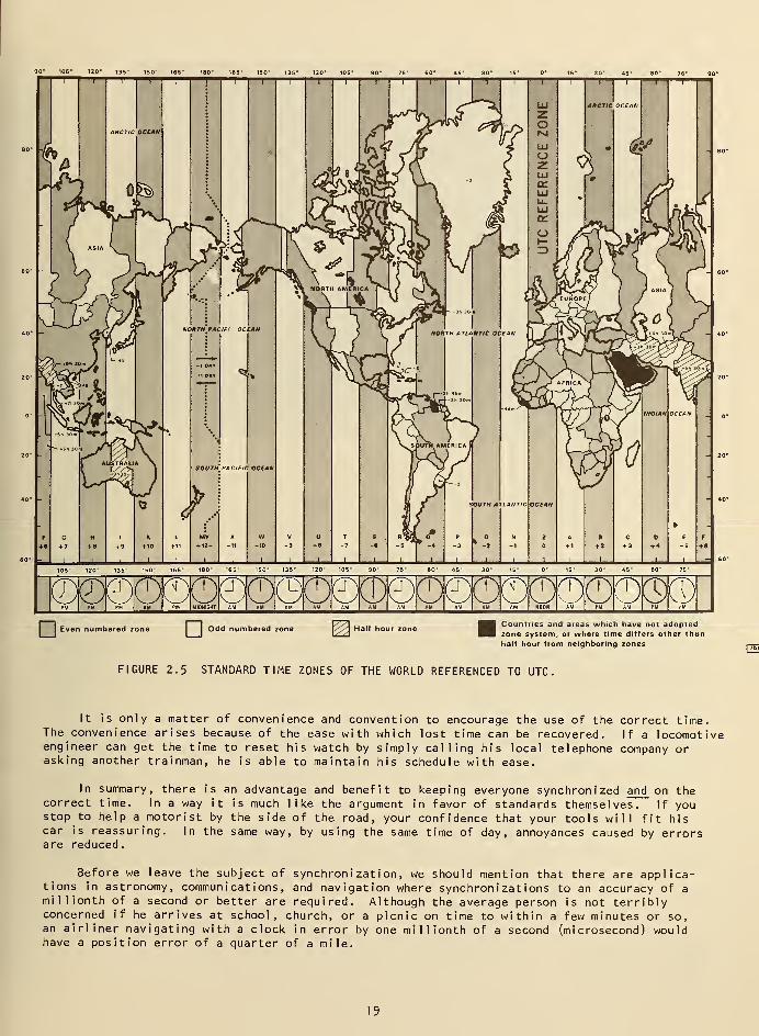
165* 150* 135* 120* 105° 90" 75" 60* 45° 30° 15°
T15" 30° 45° 60° 75* 90°
105" 120° 135" 150° 165° 1B0* 165° 150° 135° 120° 105* 90° 75° 60° 45* 30° 15* 0" 15* 30° 45° 60* 75*
I Even numbered zone '
I Odd numbered zone Half hour zoneCountries and areas which have not adoptedzone system, or where time differs other thanhalf hour from neighboring zones.
[7E>
FIGURE 2.5 STANDARD TIME ZONES OF THE WORLD REFERENCED TO UTC
.
It is only a matter of convenience and convention to encourage the use of the correct time.The convenience arises because of the ease with which lost time can be recovered. If a locomotiveengineer can get the time to reset his watch by simply calling his local telephone company orasking another trainman, he is able to maintain his schedule with ease.
In summary, there is an advantage and benefit to keeping everyone synchronized and on thecorrect time. In a way it is much like the argument in favor of standards themselves. If youstop to help a motorist by the side of the road, your confidence that your tools will fit hiscar is reassuring. In the same way, by using the same time of day, annoyances caused by errorsare reduced.
Before we leave the subject of synchronization, we should mention that there are applica-tions in astronomy, communications, and navigation where synchronizations to an accuracy of amillionth of a second or better are required. Although the average person is not terriblyconcerned if he arrives at school, church, or a picnic on time to within a few minutes or so,an airliner navigating with a clock in error by one millionth of a second (microsecond) wouldhave a position error of a quarter of a mile.
19
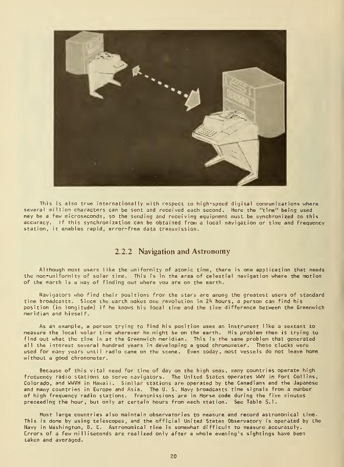
This is also true internationally with respect to high-speed digital communications whereseveral million characters can be sent and received each second. Here the "time" being usedmay be a few microseconds, so the sending and receiving equipment must be synchronized to thisaccuracy. If this synchronization can be obtained from a local navigation or time and frequencystation, it enables rapid, error-free data transmission.
2.2.2 Navigation and Astronomy
Although most users like the uniformity of atomic time, there is one application that needsthe non-uniformity of solar time. This is in the area of celestial navigation where the motionof the earth is a way of finding out where you are on the earth.
Navigators who find their positions from the stars are among the greatest users of standardtime broadcasts. Since the earth makes one revolution in 2k hours, a person can find his
position (in longitude) if he knows his local time and the time difference between the Greenwichmeridian and himself.
As an example, a person trying to find his position uses an instrument like a sextant to
measure the local solar time wherever he might be on the earth. His problem then is trying to
find out what the time is at the Greenwich meridian. This is the same problem that generatedall the interest several hundred years in developing a good chronometer. These clocks wereused for many years until radio came on the scene. Even today, most vessels do not leave home
without a good chronometer.
Because of this vital need for time of day on the high seas, many countries operate high
frequency radio stations to serve navigators. The United States operates WWV in Fort Collins,
Colorado, and WWVH in Hawaii. Similar stations are operated by the Canadians and the Japanese
and many countries in Europe and Asia. The U. S. Navy broadcasts time signals from a number
of high frequency radio stations. Transmissions are in Morse code during the five minutespreceeding the hour, but only at certain hours from each station. See Table 5-1.
Most large countries also maintain observatories to measure and record astronomical time.
This is done by using telescopes, and the official United States Observatory is operated by the
Navy in Washington, D. C. Astronomical time is somewhat difficult to measure accurately.Errors of a few milliseconds are realized only after a whole evening's sightings have been
taken and averaged.
20
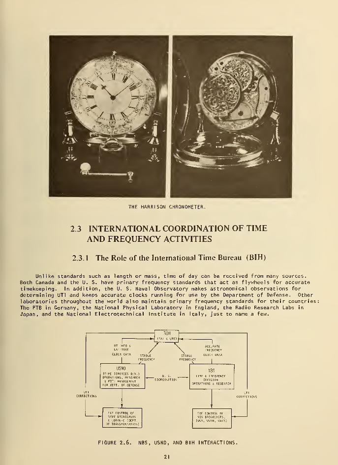
THE HARRISON CHRONOMETER.
2.3 INTERNATIONAL COORDINATION OF TIMEAND FREQUENCY ACTIVITIES
2.3. 1 The Role of the International Time Bureau (BIH)
Unlike standards such as length or mass, time of day can be received from many sources.Both Canada and the U. S. have primary frequency standards that act as flywheels for accuratetimekeeping. In addition, the U. S. Naval Observatory makes astronomical observations for
determining UT1 and keeps accurate clocks running for use by the Department of Defense. Otherlaboratories throughout the world also maintain primary frequency standards for their countriesThe PTB in Germany, the National Physical Laboratory in England, the Radio Research Labs in
Japan, and the National Electrotechnical Institute in Italy, just to name a few.
UTI
CORRECTIONS
BIH
(TAI £ UTC)
UT INFO £
LATITUDE
CLOCK DATA STABLE
FREQUENCY
USNO
(TIME SERVICES DIV.)OPERATIONS, RESEARCH£ PTTI MANAGEMENT
FOR DEPT. OF DEFENSE
TE.F CONTROL OFNAVY BROADCASTS£ LORAN-C (DEPT.
OF TRANSPORTATION)
STABLEFREQUENCY
ACCURATEFREQUENCY
CLOCK DATA
COORDINATION
NBS
TIME £ FREQUENCYOIVISION
OPERATIONS £ RESEARCH
UTI
CORRECTIONS
T£F CONTROL OFNBS BROADCASTS,(UUV, WWVH, UWVB)
FIGURE 2.6. NBS, USNO, AND BIH INTERACTIONS,
21
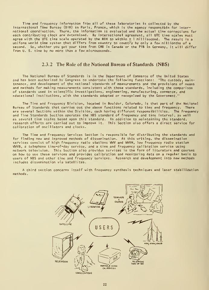
Time and frequency information from all of these laboratories is collected by theInternational Time Bureau (BIH) in Paris, France, which is the agency responsible for inter-national coordination. There, the information is evaluated and the actual time corrections foreach contributing clock are determined. By international agreement, all UTC time scales mustagree with the UTC time scale operated by the BIH to within + 1 millisecond. The result is a
uniform world time system that differs from country to country by only a few millionths of a
second. So, whether you get your time from CHU in Canada or the PTB in Germany, it will differfrom U. S. time by no more than a few microseconds.
2.3.2 The Role of the National Bureau of Standards (NBS)
The National Bureau of Standards is in the Department of Commerce of the United Statesand has been authorized by Congress to undertake the following functions: "The custody, main-tenance, and development of the national standards of measurements and the provisions of meansand methods for making measurements consistent with those standards, including the comparisonof standards used in scientific investigations, engineering, manufacturing, commerce, andeducational institutions, with the standards adopted or recognized by the Government,"
The Time and Frequency Division, located in Boulder, Colorado, is that part of the NationalBureau of Standards that carries out the above functions related to time and frequency. Thereare several Sections within the Division, each having different responsibilities. The Frequencyand Time Standards Section operates the NBS standard of frequency and time interval, as well
as several time scales based upon this standard. In addition to maintaining the standard,research efforts are carried out to improve it. This Section also offers a direct service for
calibration of oscillators and clocks.
The Time and Frequency Services Section is responsible for distributing the standards and
for finding new and improved methods of dissemination. At this writing, the disseminationservices consist of high frequency radio stations WWV and WWVH, low frequency radio stationWWVB, a telephone time-of-day service, and a time and frequency calibration service using
network television. This Section also provides services in the form of literature and courseson how to use these services and provides calibration and monitoring data on a regular basis to
users of NBS and other time and frequency services. Research and development into new methodsincludes dissemination via satellites.
A third section concerns itself with frequency synthesis techniques and laser stabilizationmethods
.
<5£MiNAe<;
COUKES
M4
SATELLITE
/hiVI—- PORTABLE CLOCK
[l__\ CALIBRAT.OW
GOUqUlTATIOMS
TELEPHONETIM£-Of=-OAY
22
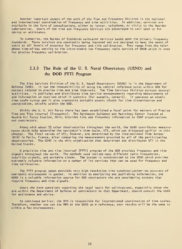
Another important aspect of the work of the Time and Frequency Division is the nationaland international coordination of frequency and time activities. In addition, services areavailable in the form of consultations, either by letter, telephone, or visits to the BoulderLaboratories. Users of the time and frequency services are encouraged to call upon us foradvice or assistance.
To summarize, the Bureau of Standards maintains services based upon the primary frequencystandards. These services are constantly being improved and are designed to meet the needs ofusers at all levels of accuracy for frequency and time calibration. They range from the tele-phone time-of-day service to the ultra-stable low frequency radio service of WWVB which is usedfor precise frequency calibration.
2.3.3 The Role of the U. S. Naval Observatory (USNO) and
the DOD PTTI Program
The Time Services Division of the U. S. Naval Observatory (USNO) is in the Department ofDefense (DOD). It has the responsibility of being the central reference point within DOD for
matters related to precise time and time intervals. The Time Services Division pursues severalactivities. It publishes and distributes time service announcements regarding measurements of
and information on stations which it controls (for example, Loran-C) . It operates an atomictime scale system and it also transports portable atomic clocks for time dissemination andcoordination, chiefly within the DOD.
Within the U. S. Air Force there has been established a focal point for matters of PreciseTime and Time Interval (frequency). The Aerospace Guidance and Metrology Center located atNewark Air Force Station, Ohio, provides time and frequency information to USAF organizationsand contractors.
Along with about 75 other observatories throughout the world, the USNO contributes measure-ments which help determine the navigator's time scale, UT1 , which was discussed earlier in this
chapter. The final values of UT1 , however, are determined by the International Time Bureau(BIH) in Paris, France, after comparing the measurements provided by all of the participatingobservatories. The USNO is the only organization that determines and distributes UT1 in the
United States.
A precision time and time interval (PTTI) program of the DOD provides frequency and time
signals throughout the world. The methods used include many different radio frequencies,satellite signals, and portable clocks. The system is synchronized to the USNO which providesextremely valuable information on a number of its services that can be used for frequency and
time cal i brat ion
.
The PTTI program makes possible very high resolution time synchroni zat ion--an accuracy of
one-tenth microsecond is quoted. In addition to monitoring and publishing information, the
USNO is a valuable information source for DOD contractors who are considering systems that
require frequency and time signals.
Users who have questions regarding the legal basis for calibrations, especially those whoare within the Department of Defense or contractors to that Department, should consult the USNO
for assistance and advice.
As mentioned earlier, the BIH is responsible for international coordination of time scales.
Therefore, whether you use the NBS or the USNO as a reference, your results will be the same to
within a few microseconds.
23
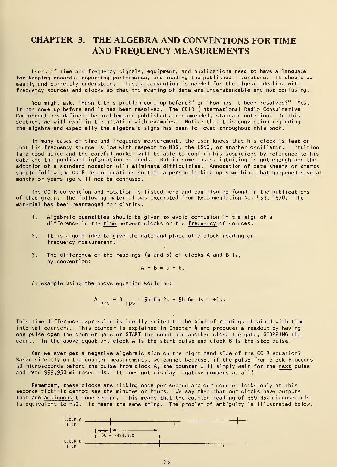
CHAPTER 3. THE ALGEBRA AND CONVENTIONS FOR TIMEAND FREQUENCY MEASUREMENTS
Users of time and frequency signals, equipment, and publications need to have a language
for keeping records, reporting performance, and reading the published literature. It should be
easily and correctly understood. Thus, a convention is needed for the algebra dealing with
frequency sources and clocks so that the meaning of data are understandable and not confusing.
You might ask, "Hasn't this problem come up before?" or "How has it been resolved?" Yes,
it has come up before and it has been resolved. The CC 1 R (International Radio ConsultativeCommittee) has defined the problem and published a recommended, standard notation. In this
section, we will explain the notation with examples. Notice that this convention regarding
the algebra and especially the algebraic signs has been followed throughout this book.
In many cases of time and frequency measurement, the user knows that his clock is fast or
that his frequency source is low with respect to NBS, the USNO, or another oscillator. Intuition
is a good guide and the careful worker will be able to confirm his suspicions by reference to his
data and the published information he needs. But in some cases, intuition is not enough and the
adoption of a standard notation will eliminate difficulties. Annotation of data sheets or chartsshould follow the CC I R recommendations so that a person looking up something that happened several
months or years ago will not be confused.
The CC I R convention and notation is listed here and can also be found in the publicationsof that group. The following material was excerpted from Recommendation No. k$3 , 1970. The
material has been rearranged for clarity.
1. Algebraic quantities should be given to avoid confusion in the sign of a
difference in the time between clocks or the frequency of sources.
2. It is a good idea to give the date and place of a clock reading orfrequency measurement.
3. The difference of the readings (a and b) of clocks A and B is,
by convention:A - B = a - b.
An example using the above equation would be:
A. - B. = 5h 6m 2s - 5h 6m Is = +ls.lpps lpps
This time difference expression is ideally suited to the kind of readings obtained with timeinterval counters. This counter is explained in Chapter h and produces a readout by havingone pulse open the counter gate or START the count and another close the gate, STOPPING the
count. In the above equation, clock A is the start pulse and clock B is the stop pulse.
Can we ever get a negative algebraic sign on the right-hand side of the CCIR equation?Based directly on the counter measurements, we cannot because, if the pulse from clock B occurs50 microseconds before the pulse from clock A, the counter will simply wait for the next pulseand read 999,950 microseconds. It does not display negative numbers at all!
Remember, these clocks are ticking once per second and our counter looks only at thisseconds tick--it cannot see the minutes or hours. We say then that our clocks have outputsthat are ambiguous to one second. This means that the counter reading of 999,950 microsecondsis equivalent to -50. It means the same thing. The problem of ambiguity is illustrated below.
CLOCK A
TICK
CLOCK B
TICK
I
-50 = +999,950
25
Another example, showing the correct notation that should be used, follows. This could be
the result obtained by carrying an NBS portable clock to the U. S. Naval Observatory and measuringit against the USNO clock. The results of this comparison are properly written:
NBS PORTABLE CLOCK - UTC(USNO) = + 12.3 MICROSECONDS (7 JULY 68, lAh 35m; UTC).
There can be no confusion about the meaning of this measurement providing the whole expressionis recorded. Do not simply make a claim that the NBS portable clock leads, lags, is fast or
slow, or ahead or behind of the USNO clock. The algebraic expression should be used!
It is also important to follow the notation for frequency differences. Terms like high,
low, and offset should be avoided. Since the algebra speaks for itself, it should be used
with a minimum of additional terms.
3.1 EXPRESSING FREQUENCY DIFFERENCE (IN HERTZ, kHz, MHz, ETC.)
The actual frequency of a source is indicated by the lowercase letter, f. (Refer to the
glossary at the end of this book for a further explanation and definition.) A subscript can
be used to identify the particular frequency source; e.g., f c for an oscillator designated "c."Multiple letter subscripts are sometimes used as in the case of NBS, USNO, ABC, NBC, and CBS.
With this notation, we can write:
f, - f
h= Af '
a b
where Af is the frequency difference in hertz, kHz, Mhz, etc.
The significance of this seemingly simple expression must be stressed. This is the actual
frequency coming out of the source (e.g., oscillator) and not the nominal frequency, f n , that
is written on the manufacturer's nameplate or in the specifications. However, it is useful to
note the nominal frequency, f , of the source when writing down this measurement result.
3.2 RELATIVE (FRACTIONAL) FREQUENCY, F (DIMENSIONLESS)
The term "fractional," though in common use throughout the English-speaking world, is beingdiscouraged by the CC I R because of difficulties in translating that term into certain otherlanguages. The CCIR prefers the use of "relative" or "normalized" rather than "fractional."We have reflected this throughout the text.
The relative frequency departure of frequency source "c," for instance, from its nominalvalue f is defined as:
nc
f
F = t 1 (which i s di mens ion less)
,
nc
where F is the designation for relative frequency.
This expression can be rearranged:
(fc
- f )
F = t (dimens ionless)
.
c fnc
It now has the form j— which is often used in frequency measurements and computations. Be verycareful to note the exact order of the terms in the numerator!
26
3.3 RELATIVE (FRACTIONAL) FREQUENCY DIFFERENCE,S (DIMENSIONLESS)
We can apply the formula in the above equation to two separate frequency sources and then
take a difference in that quantity. It will.be the relative frequency difference between two
sources. For example, consider sources NBS and USNO.
S = FNBS " F
USN0'
where S is the relative frequency difference.
Let's assume that an NBS oscillator was measured against a USNO oscillator. The resultscould be written as:
FNBS
" FUSN0
= +5 x ,0" 13
(7 July 1968, ]k h 35 min to 20 h 30 min UTC ; USNO).
This, then, is a complete, unambiguous statement about the frequencies of two sources.There is a general temptation to use the resulting algebraic signs from such calibrations andmake statements about such and such a frequency source being low or high relative to another.The examples using this notation shown below illustrate the difficulty in making such statements
3.3.1 Example of Algebra and Sign Conventions in Time and Frequency Measurements
A. Television Frequency Transfer Measurements (covered in Chapter 7)
The NBS Time and Frequency Services Bulletin reports the measured values of the threemajor U. S. networks. On page 140 of this book, a portion of that bulletin shows typical dataobtained from the TV measurements. Let's look more closely at this data.
The heading for the data is labeled "RELATIVE FREQUENCY (in parts in 1011
)." Followingthe CCIR convention, then, these data represent F.,,,., F. m _, and FrDC .
Expressing the first NBC reading in equation form, using the -=— arrangement:
FNBC
=fNBC
- fNBC(nominal) = ^^ x 1Q
-11
NBC (nominal
)
What does this tell us? If we assume we are dealing with a frequency source at 5 MHz, we can
substitute that number for the nominal frequency and solve for the actual frequency of the
signal being received from NBC via the TV color subcarrier:
f - (5 x 10⁶
)
FNBC =— 1 "
" 3019 - /t X 10 •
NBC5 x 10
6
Using the equality on the right:
fNBC
" (5 X 1q6) = "3019.'* x 10" 11x 5 x 10
6,
fNBC " (5 X 1q6) = " 15°97 X 10
"5,
fNBC
= 5 x 10⁶
- 0.15097 Hz.
27
ie
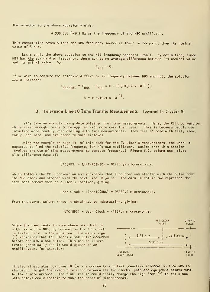
The solution to the above equation yields:
4, 999, 999. 84903 Hz as the frequency of the NBC oscillator.
This computation reveals that the NBC frequency source is lower in frequency than its nominalvalue of 5 MHz.
Let's apply the above equation to the NBS frequency standard itself. By definition, sinceNBS has the standard of frequency, there can be no average difference between its nominal valueand its actual value. So:
FNBS " °«
If we were to compute the relative difference in frequency between NBS and NBC, the solutionwould indicate:
SNBS-NBC=
FNBS
" FNBC=° " (-3019-4 X lO"11
).
S = + 3019-4 x lO"11
.
B. Television Line- 10 Time Transfer Measurements, (covered in Chapter 8)
Let's take an example using data obtained from time measurements. Here, the CCIR convention,while clear enough, needs to be applied with more care than usual. This is because people useintuition more readily when dealing with time measurements. They feel at home with fast, slow,early, and late, and are prone to make mistakes.
Using the example on page 141 of this book for the TV Line-10 measurements, the user is
expected to find the relative frequency for his own oscillator. Notice that this probleminvolves the use of time measurements to compute frequency! Figure 8.7, column one, givestime difference data of:
UTC(NBS) - LINE-IO(NBC) = 02216.54 microseconds,
which follows the CCIR convention and indicates that a counter was started with the pulse from
the NBS clock and stopped with the next Line-10 pulse. The data in column two represent the
same measurement made at a user's location, giving:
User Clock - Line-IO(NBC) = 05339-9 microseconds.
From the above, column three is obtained, by subtraction, giving:
UTC(NBS) - User Clock = -3123-4 microseconds.
NBS CLOCK LINE-10
P . .. , , , . , , - PULSE PULSESince the user wants to know where his clock is
with respect to NBS, by convention the NBS clock 11
is listed first in the equation. The minus sign It' '
(-) indicates that the user's clock pulse occurred 1
3 ' 23 ' 4 ys
[
.2216 -^ ms
^1
before the NBS clock pulse. This can be 1 1 1 us-5,,a
g U5
trated graphically (as it would appear on an,
* »|
oscilloscope, for example):USER'S LINE-10
CLOCK PULSE PULSE
It also illustrates how Line-10 (or any common time pulse) transfers information from NBS to
the user. To get the exact time error between the two clocks, path and equipment delays must
be taken into account. The final result could easily change the sign from (-) to (+) since
path delays could contribute many thousands of microseconds.
28
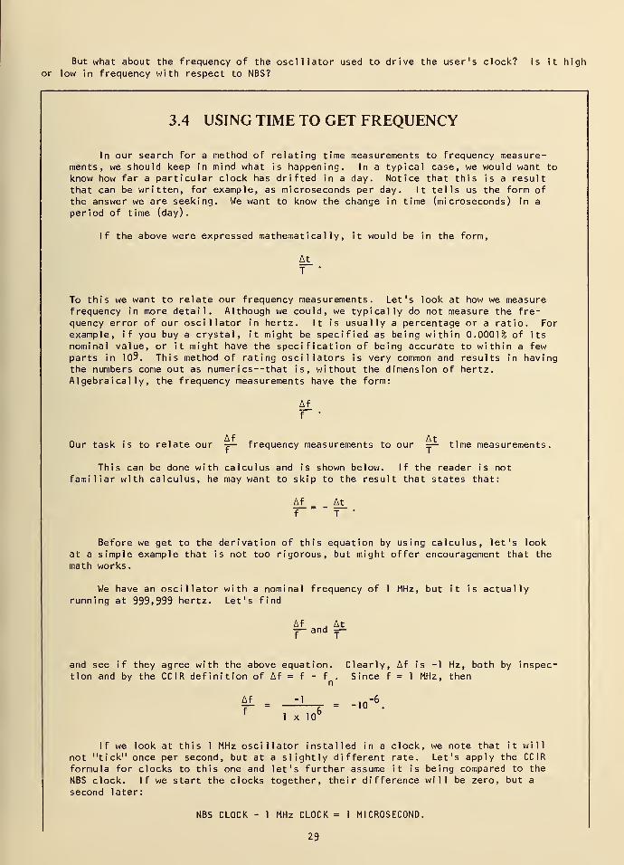
But what about the frequency of the oscillator used to drive the user's clock? Is it highor low in frequency with respect to NBS?
3.4 USING TIME TO GET FREQUENCY
In our search for a method of relating time measurements to frequency measure-ments, we should keep in mind what is happening. In a typical case, we would want to
know how far a particular clock has drifted in a day. Notice that this is a result
that can be written, for example, as microseconds per day. It tells us the form of
the answer we are seeking. We want to know the change in time (microseconds) in a
period of time (day).
If the above were expressed mathematically, it would be in the form,
AtT
*
To this we want to relate our frequency measurements. Let's look at how we measurefrequency in more detail. Although we could, we typically do not measure the fre-quency error of our oscillator in hertz. It is usually a percentage or a ratio. For
example, if you buy a crystal, it might be specified as being within 0.0001% of its
nominal value, or it might have the specification of being accurate to within a fewparts in 109. This method of rating oscillators is very common and results in havingthe numbers come out as numer ics--that is, without the dimension of hertz.Algebraically, the frequency measurements have the form:
Aff *
,Af - At
Our task is to relate our =— frequency measurements to our =— time measurements.
This can be done with calculus and is shown below. If the reader is notfamiliar with calculus, he may want to skip to the result that states that:
Af Atf " T '
Before we get to the derivation of this equation by using calculus, let's lookat a simple example that is not too rigorous, but might offer encouragement that themath works
.
We have an oscillator with a nominal frequency of 1 MHz, but it is actuallyrunning at 999,999 hertz. Let's find
Af . At— and —
and see if they agree with the above equation. Clearly, Af is -1 Hz, both by inspec-tion and by the CCIR definition of Af = f - f . Since f = 1 MHz, then
n
« , _^i . -,o-6
.
f1 X 10
6
If we look at this 1 MHz oscillator installed in a clock, we note that it will
not "tick" once per second, but at a slightly different rate. Let's apply the CCIR
formula for clocks to this one and let's further assume it is being compared to the
NBS clock. If we start the clocks together, their difference will be zero, but a
second later:
NBS CLOCK - 1 MHz CLOCK = 1 MICROSECOND.
29
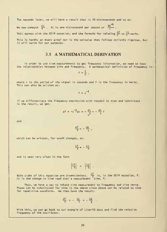
Ten seconds later, we will have a resu t that is 10 microseconds and so on.
,iA t ... • a
1°~6
we now compute — . It is one microsecond per second or —:.
This agrees with the CCIR notation, and the formula for relatinq =— to =— works.3f T
This is hardly an exact proof nor is the calculus that follows strictly rigorous, butit will serve for our purposes.
3.5 A MATHEMATICAL DERIVATION
In order to use time measurements to get frequency information, we need to knowthe relationships between time and frequency. A mathematical definition of frequency is:
where t is the period of the signal in seconds and f is the frequency in hertz.This can also be written as:
f-t" 1
.
If we differentiate the frequency expression with respect to time and substitutein the result, we get:
df = -t
" 2dt - -
d!j
= -d\ f
and
df dt
f t'
which can be written, for small changes, as:
Af Atf " T
and is seen very often in the form
Af
f= At
T•
Both sides of this equation are d imensionless . —=- is, in the CCIR notation, F.
At is the change in time read over a measurement time, T.
Thus, we have a way to relate time measurement to frequency and vice versa.Phase can be substituted for time in the above since phase can be related to timefor repetitive waveforms. We then have the result:
Af At A(j>
f T<J>
"
With this, we can go back to our example of Line-10 data and find the relativefrequency of the oscillator.
30
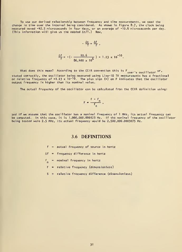
To use our derived relationship between frequency and time measurements, we need thechange in time over the interval being considered. As shown in figure 8.7, the clock beingmeasured moved -hi. 5 microseconds in four days, or an average of -10.6 microseconds per day.(This information will give us the needed At/T.) Now,
At_ = Af_
T f'
Af , 10.6 , . ., ,.-10-s- = -( r ) = 1.23 x 10
86,400 x 10
What does this mean? According to the CC I R convention this is F . .,, or,user 's osci 1 lator
stated correctly, the oscillator being measured using Line-10 TV measurements has a fractionalor relative frequency of +1.23 x 10"10. The plus sign (+) on F indicates that the oscillatoroutput frequency is higher than its nominal value.
The actual frequency of the oscillator can be calculated from the CC I R definition using:
f - f
F =fn
and if we assume that the oscillator has a nominal frequency of 1 MHz, its actual frequency canbe computed. In this case, it is 1,000,000.000123 Hz. If the nominal frequency of the oscillatorbeing tested were 2.5 MHz, its actual frequency would be 2,500,000.0003075 Hz.
3.6 DEFINITIONS
f = actual frequency of source in hertz
Af = frequency difference in hertz
f = nominal frequency in hertz
F = relative frequency (dimens ionless)
S = relative frequency difference (dimensionless)
31
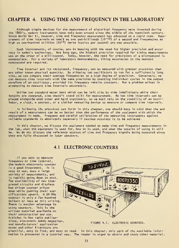
CHAPTER 4. USING TIME AND FREQUENCY IN THE LABORATORY
Although simple devices for the measurement of electrical frequency were invented duringthe 1800's, modern instruments have only been around since the middle of the twentieth century.Since World War II, however, time and frequency measurement has advanced at a rapid rate. Meas-urement of time intervals as small as one ten-billionth (10~10) of a second and frequencies as
high as one-hundred trillion (10^) hertz (cycles per second) are now possible.
Such improvements, of course, are in keeping with the need for higher precision and accu-racy in today's technology. Not long ago, the highest precision required for timing measurementswas on the order of a millisecond. Today, however, the need for precisions of a microsecond is
commonplace. For a variety of laboratory measurements, timing accuracies to the nearestnanosecond are required.
Time interval and its reciprocal, frequency, can be measured with greater precision than
any other known physical quantity. By allowing two oscillators to run for a sufficiently long
time, we can compare their average frequencies to a high degree of precision. Conversely, wecan measure time intervals with the same precision by counting individual cycles in the outputwaveform of an oscillator, provided its frequency remains constant. But a problem arises in
attempting to measure time intervals accurately.
Unlike two standard meter bars which can be left side by side indefinitely while their
lengths are compared, time doesn't stand still for measurement. No two time intervals can be
placed alongside each other and held stationary, so we must rely on the stability of an oscil-lator, a clock, a counter, or a similar measuring device to measure or compare time intervals.
In following the practices set forth in this chapter, one should keep in mind that the end
result of a measurement can be no better than the performance of the equipment with which themeasurement is made. Frequent and careful calibration of the measuring instruments againstreliable standards is absolutely necessary if maximum accuracy is to be achieved.
In this chapter, we discuss the equipment needed to make time and frequency measurements in
the lab, what the equipment is used for, how it is used, and what the results of using it will
be. We do not discuss the reference sources of time and frequency signals being measured sincethey are fully discussed in later chapters.
4.1 ELECTRONIC COUNTERS
If you want to measurefrequency or time interval,the modern electronic counteris a good investment. It is
easy to use, does a largevariety of measurements, and
is rapidly going down in cost.The availability of new inte-
grated circuits and displayshas driven counter pricesdown while pushing their spe-cifications upward. A 50 MHzcounter is only a few hundreddollars or less at this writing.There is another advantage in
using counters. This is the
written material available on
their construction and use.
Articles in Ham radio publica-tions, electronic hobby magazines,and manufacturers' applicationnotes and other literature areplentiful, easy to find, and easy to read. In this chapter, only part of the availablmation is presented in a tutorial way. The reader is urged to obtain and study other
FIGURE 4. 1 . ELECTRONIC COUNTERS.
e infor-mater ial
33
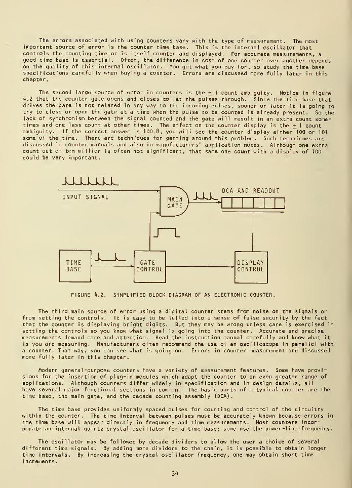
The errors associated with using counters vary with the type of measurement. The mostimportant source of error is the counter time base. This is the internal oscillator thatcontrols the counting time or is itself counted and displayed. For accurate measurements, a
good time base is essential. Often, the difference in cost of one counter over another dependson the quality of this internal oscillator. You get what you pay for, so study the time basespecifications carefully when buying a counter. Errors are discussed more fully later in thischapter.
The second large source of error in counters is the + 1 count ambiguity. Notice in figure*4.2 that the counter gate opens and closes to let the pulses through. Since the time base thatdrives the gate is not related in any way to the incoming pulses, sooner or later it is going totry to close or open the gate at a time when the pulse to be counted is already present. So thelack of synchronism between the signal counted and the gate will result in an extra count some-times and one less count at other times. The effect on the counter display is the + 1 countambiguity. If the correct answer is 100.8, you will see the counter display either""100 or 101
some of the time. There are techniques for getting around this problem. Such techniques arediscussed in counter manuals and also in manufacturers' application notes. Although one extracount out of ten million is often not significant, that same one count with a display of 100could be very important.
JJJJJJJ^.
INPUT SIGNALDCA AND READOUT
GATECONTROL
J—
L
DISPLAYCONTROL
FIGURE k.2. SIMPLIFIED BLOCK DIAGRAM OF AN ELECTRONIC COUNTER.
The third main source of error using a digital counter stems from noise on the signals or
from setting the controls. It is easy to be lulled into a sense of false security by the fact
that the counter is displaying bright digits. But they may be wrong unless care is exercised in
setting the controls so you know what signal is going into the counter. Accurate and precisemeasurements demand care and attention. Read the instruction manual carefully and know what it
is you are measuring. Manufacturers often recommend the use of an oscilloscope in parallel witha counter. That way, you can see what is going on. Errors in counter measurement are discussedmore fully later in this chapter.
Modern general -purpose counters have a variety of measurement features. Some have provi-sions for the insertion of plug-in modules which adapt the counter to an even greater range ofapplications. Although counters differ widely in specification and in design details, all
have several major functional sections in common. The basic parts of a typical counter are the
time base, the main gate, and the decade counting assembly (DCA).
The time base provides uniformly spaced pulses for counting and control of the circuitrywithin the counter. The time interval between pulses must be accurately known because errors in
the time base will appear directly in frequency and time measurements. Most counters incor-
porate an internal quartz crystal oscillator for a time base; some use the power-line frequency.
The oscillator may be followed by decade dividers to allow the user a choice of severaldifferent time signals. By adding more dividers to the chain, it is possible to obtain longer
time intervals. By increasing the crystal oscillator frequency, one may obtain short time
increments.
3**
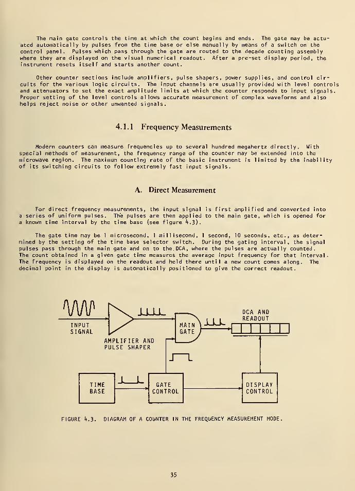
The main gate controls the time at which the count begins and ends. The gate may be actu-ated automatically by pulses from the time base or else manually by means of a switch on the
control panel. Pulses which pass through the gate are routed to the decade counting assemblywhere they are displayed on the visual numerical readout. After a pre-set display period, the
instrument resets itself and starts another count.
Other counter sections include amplifiers, pulse shapers, power supplies, and control cir-cuits for the various logic circuits. The input channels are usually provided with level controlsand attenuators to set the exact amplitude limits at which the counter responds to input signals.Proper setting of the level controls allows accurate measurement of complex waveforms and alsohelps reject noise or other unwanted signals.
4. 1 . 1 Frequency Measurements
Modern counters can measure frequencies up to several hundred megahertz directly. Withspecial methods of measurement, the frequency range of the counter may be extended into the
microwave region. The maximum counting rate of the basic instrument is limited by the inabilityof its switching circuits to follow extremely fast input signals.
A. Direct Measurement
For direct frequency measurements, the input signal is first amplified and converted into
a series of uniform pulses. The pulses are then applied to the main gate, which is opened for
a known time interval by the time base (see figure **.3).
The gate time may be 1 microsecond, 1 millisecond, 1 second, 10 seconds, etc., as deter-mined by the setting of the time base selector switch. During the gating interval, the signalpulses pass through the main gate and on to the.DCA, where the pulses are actually counted.The count obtained in a given gate time measures the average input frequency for that interval.The frequency is displayed on the readout and held there until a new count comes along. Thedecimal point in the display is automatically positioned to give the correct readout.
wINPUTSIGNAL
±1±L.
AMPLIFIER ANDPULSE SHAPER
i-Lk.
DCA ANDREADOUT
J—
L
DISPLAYCONTROL
FIGURE k.3. DIAGRAM OF A COUNTER IN THE FREQUENCY MEASUREMENT MODE,
35
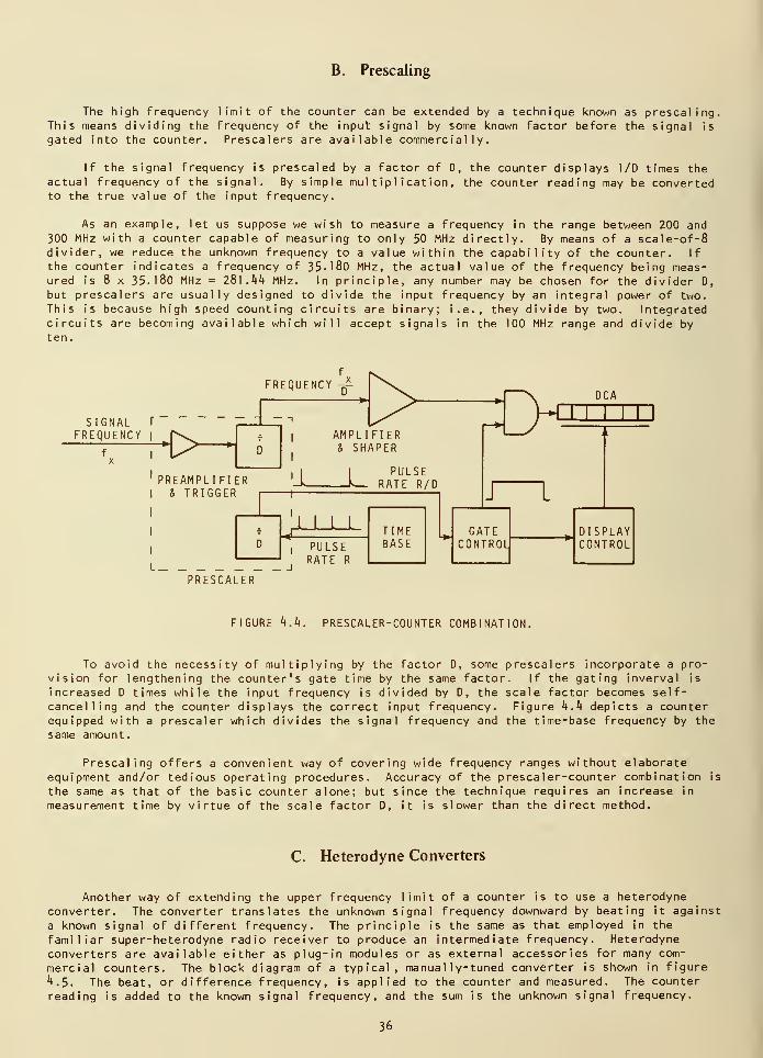
B. Prescaling
The high frequency limit of the counter can be extended by a technique known as prescaling.This means dividing the frequency of the input signal by some known factor before the signal is
gated into the counter. Prescalers are available commercially.
If the signal frequency is prescaled by a factor of D, the counter displays 1/D times theactual frequency of the signal. By simple multiplication, the counter reading may be convertedto the true value of the input frequency.
As an example, let us suppose we wish to measure a frequency in the range between 200 and300 MHz with a counter capable of measuring to only 50 MHz directly. By means of a scale-of-8divider, we reduce the unknown frequency to a value within the capability of the counter. If
the counter indicates a frequency of 35-180 MHz, the actual value of the frequency being meas-ured is 8 x 35.180 MHz = 281. kk MHz. In principle, any number may be chosen for the divider D,
but prescalers are usually designed to divide the input frequency by an integral power of two.
This is because high speed counting circuits are binary; i.e., they divide by two. Integratedcircuits are becoming available which will accept signals in the 100 MHz range and divide by
ten.
SIGNAL T
FREQUENCY
DISPLAYCONTROL
PRESCALER
FIGURE k.k. PRESCALER-COUNTER COMBINATION.
To avoid the necessity of multiplying by the factor D, some prescalers incorporate a pro-vision for lengthening the counter's gate time by the same factor. If the gating inverval is
increased D times while the input frequency is divided by D, the scale factor becomes self-cancelling and the counter displays the correct input frequency. Figure k.k depicts a counterequipped with a prescaler which divides the signal frequency and the time-base frequency by the
same amount.
Prescaling offers a convenient way of covering wide frequency ranges without elaborateequipment and/or tedious operating procedures. Accuracy of the prescaler-counter combination is
the same as that of the basic counter alone; but since the technique requires an increase in
measurement time by virtue of the scale factor D, it is slower than the direct method.
C. Heterodyne Converters
Another way of extending the upper frequency limit of a counter is to use a heterodyneconverter. The converter translates the unknown signal frequency downward by beating it aga
a known signal of different frequency. The principle is the same as that employed in the
familiar super-heterodyne radio receiver to produce an intermediate frequency. Heterodyneconverters are available either as plug-in modules or as external accessories for many com-
mercial counters. The block diagram of a typical, manually-tuned converter is shown in figure
^.5. The beat, or difference frequency, is applied to the counter and measured. The counterreading is added to the known signal frequency, and the sum is the unknown signal frequency.
nst
36
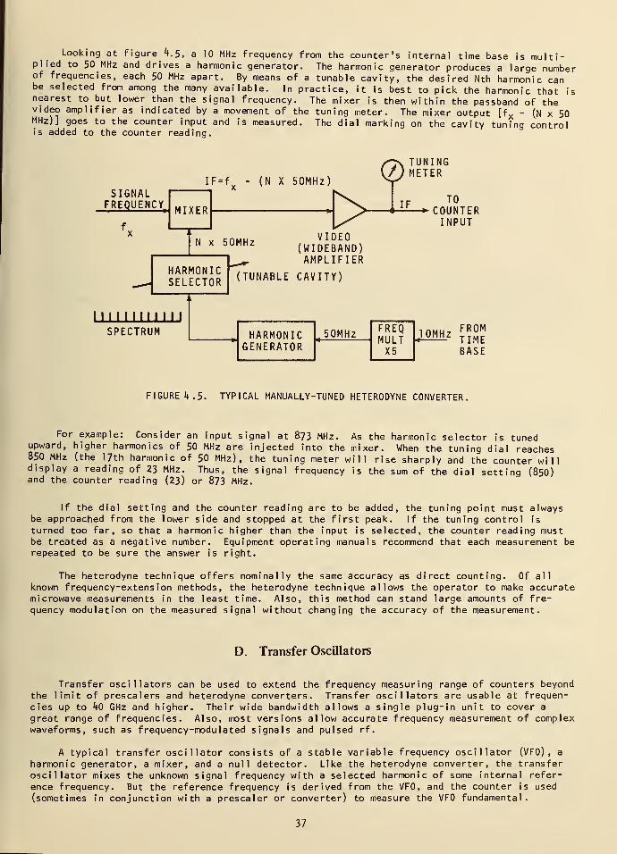
Looking at figure h.$, a 10 MHz frequency from the counter's internal time base is multi-plied to 50 MHz and drives a harmonic generator. The harmonic generator produces a large numberof frequencies, each 50 MHz apart. By means of a tunable cavity, the desired Nth harmonic canbe selected from among the many available. In practice, it is best to pick the harmonic that isnearest to but lower than the signal frequency. The mixer is then within the passband of thevideo amplifier as indicated by a movement of the tuning meter. The mixer output [fx
- (N x 50MHz)] goes to the counter input and is measured. The dial marking on the cavity tuning controlis added to the counter reading.
SIGNALFREQUENCE
IF=f - (N X 50MHz)
MIXER >N x 50MHz
HARMONICSELECTOR
I I I I II I I I I
SPECTRUM
VIDEO(WIDEBAND)AMPLIFIER
(TUNABLE CAVITY)
HARMONICGENERATOR
50MHz
©ITUNINGETER
IFTO
-•COUNTERINPUT
FREQMULTX5
10MHzFROMTIMEBASE
FIGURE ^. 5. TYPICAL MANUALLY-TUNED HETERODYNE CONVERTER.
For example: Consider an input signal at 8-73 MHz. As the harmonic selector is tunedupward, higher harmonics of 50 MHz are injected into the mixer. When the tuning dial reaches850 MHz (the 17th harmonic of 50 MHz), the tuning meter will rise sharply and the counter willdisplay a reading of 23 MHz. Thus, the signal frequency is the sum of the dial setting (850)and the counter reading (23) or 873 MHz.
If the dial setting and the counter reading are to be added, the tuning point must alwaysbe approached from the lower side and stopped at the first peak. If the tuning control is
turned too far, so that a harmonic higher than the input is selected, the counter reading mustbe treated as a negative number. Equipment operating manuals recommend that each measurement berepeated to be sure the answer is right.
The heterodyne technique offers nominally the same accuracy as direct counting. Of all
known frequency-extension methods, the heterodyne technique allows the operator to make accuratemicrowave measurements in the least time. Also, this method can stand large amounts of fre-quency modulation on the measured signal without changing the accuracy of the measurement.
D. Transfer Oscillators
Transfer oscillators can be used to extend the frequency measuring range of counters beyondthe limit of prescalers and heterodyne converters. Transfer oscillators are usable at frequen-cies up to h0 GHz and higher. Their wide bandwidth allows a single plug-in unit to cover a
great range of frequencies. Also, most versions allow accurate frequency measurement of complexwaveforms, such as frequency-modulated signals and pulsed rf.
A typical transfer oscillator consists of a stable variable frequency oscillator (VF0) , a
harmonic generator, a mixer, and a null detector. Like the heterodyne converter, the transferoscillator mixes the unknown signal frequency with a selected harmonic of some internal refer-
ence frequency. But the reference frequency is derived from the VF0, and the counter is used
(sometimes in conjunction with a prescaler or converter) to measure the VF0 fundamental.
37
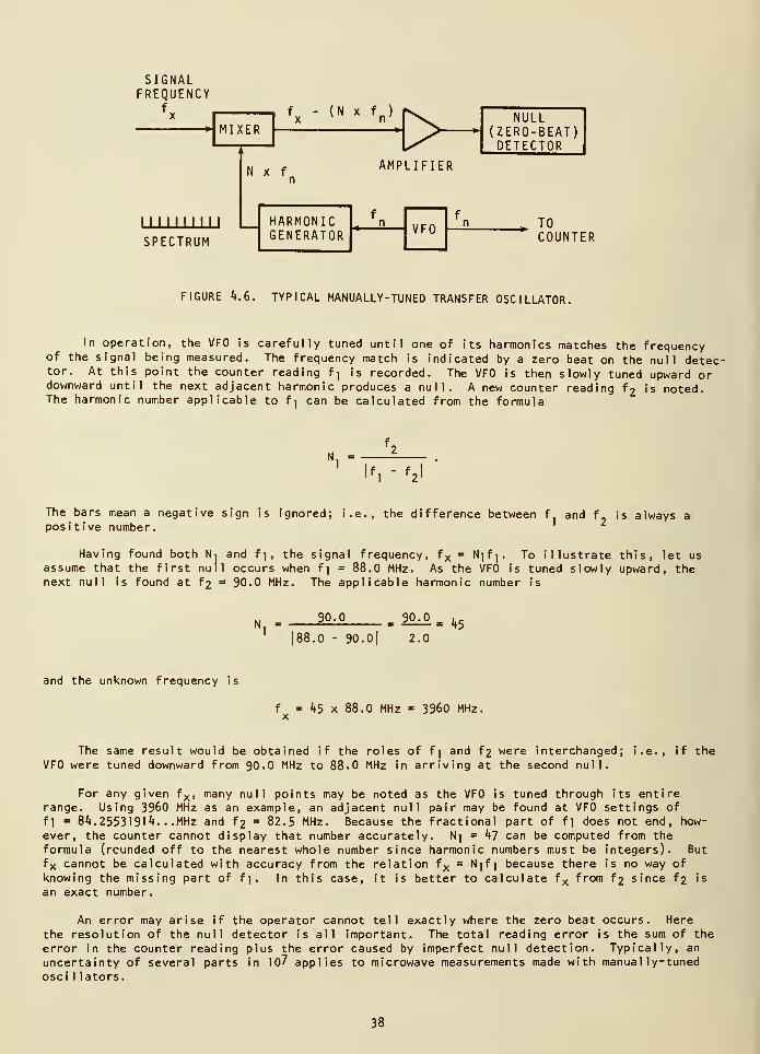
SIGNALFREQUENCY
f .
MIXER
MMMMISPECTRUM
N x f
(N x f)
HARMONICGENERATOR
H>AMPLIFIER
VFO
NULL(ZERO-BEAT)DETECTOR
TOCOUNTER
FIGURE k.6. TYPICAL MANUALLY-TUNED TRANSFER OSCILLATOR.
In operation, the VFO is carefully tuned until one of its harmonics matches the frequencyof the signal being measured. The frequency match is indicated by a zero beat on the null detec-tor. At this point the counter reading f| is recorded. The VFO is then slowly tuned upward ordownward until the next adjacent harmonic produces a null. A new counter reading f 2 is noted.The harmonic number applicable to fj can be calculated from the formula
Nl
=
If, - f2
l
The bars mean a negative sign is ignored; i.e., the difference between f. and f is always apositive number.
Having found both Ni and f,, the signal frequency, f x = Njfj. To illustrate this, let usassume that the first null occurs when f] = 88.0 MHz. As the VFO is tuned slowly upward, thenext null is found at fj = 90.0 MHz. The applicable harmonic number is
Nl
= 90.0 90.0
[88.0 - 90. 0| 2.0
= *»5
and the unknown frequency is
fx=45 .0 MHz = 3960 MHz.
The same result would be obtained if the roles of f] and f 2 were interchanged; i.e., if the
VFO were tuned downward from 90.0 MHz to 88.0 MHz in arriving at the second null.
For any given f x , many null points may be noted as the VFO is tuned through its entirerange. Using 3960 MHz as an example, an adjacent null pair may be found at VFO settings of
fl = 8^.2553191 ^. • -MHz and f2 = 82.5 MHz. Because the fractional part of fi does not end, how-ever, the counter cannot display that number accurately. N| = k~l can be computed from the
formula (rounded off to the nearest whole number since harmonic numbers must be integers). But
fx cannot be calculated with accuracy from the relation fx = Njf] because there is no way ofknowing the missing part of f 1 . In this case, it is better to calculate fx from f 2 since f 2 is
an exact number.
An error may arise if the operator cannot tell exactly where the zero beat occurs. Here
the resolution of the null detector is all important. The total reading error is the sum of the
error in the counter reading plus the error caused by imperfect null detection. Typically, an
uncertainty of several parts in 107 applies to microwave measurements made with manually-tunedosc? 1 lators.
38
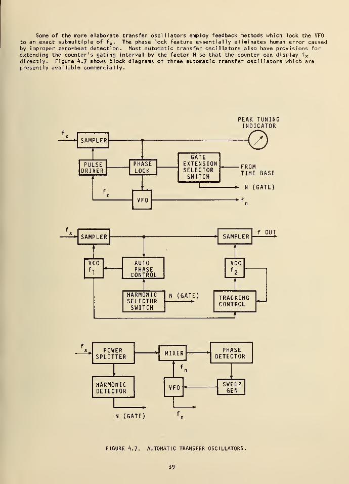
Some of the more elaborate transfer oscillators employ feedback methods which lock the VFO
to an exact submultiple of fx . The phase lock feature essentially eliminates human error causedby improper zero-beat detection. Most automatic transfer oscillators also have provisions for
extending the counter's gating interval by the factor N so that the counter can display fxdirectly. Figure k.7 shows block diagrams of three automatic transfer oscillators which arepresently available commercially.
PEAK TUNINGINDICATOR
\ /oAMrL cr\\
i
1 r GATEEXTENSIONSELECTORSWITCH
PULSEDRIVER
PHASELOCK
« Frcfmi \
1
fn
V r u ' rn
TIME BASE
fx A M ni c
f OUTb«nr lck * o n i'i r l. 1 1\
"
; L
'
I\
VCOf
l
AUTOPHASE
CONTROL
VCOf2
, ,
, i
HARMONICSELECTORSWITCH
N (GATE) TRACKINGCONTROL
' '
fx. POWER PHASE
SPLITTERn 1 A C R DETECTOR
'
i
fn
\
HARMONICDETECTOR
VFOSWEEPGEN
»
N (GATE)
FIGURE k.7. AUTOMATIC TRANSFER OSCILLATORS,
39
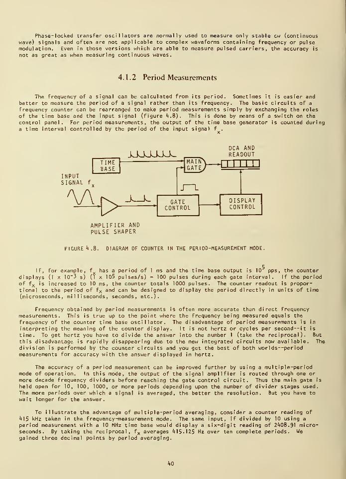
Phase-locked transfer oscillators are normally used to measure only stable cw (continuouswave) signals and often are not applicable to complex waveforms containing frequency or pulsemodulation. Even in those versions which are able to measure pulsed carriers, the accuracy is
not as great as when measuring continuous waves.
4.1.2 Period Measurements
The frequency of a signal can be calculated from its period. Sometimes it is easier and
better to measure the period of a signal rather than its frequency. The basic circuits of a
frequency counter can be rearranged to make period measurements simply by exchanging the roles
of the time base and the input signal (figure 4.8). This is done by means of a switch on the
control panel. For period measurements, the output of the time base generator is counted during
a time interval controlled by the period of the input signal f .
TIMEBASE
INPUTSIGNAL f
x
JJJJsJJ^LDCA ANDREADOUT
> X_J^ GATECONTROL
DISPLAYCONTROL
AMPLIFIER ANDPULSE SHAPER
FIGURE 4.8. DIAGRAM OF COUNTER IN THE PERIOD-MEASUREMENT MODE,
If, for example, f has a period of 1 ms and the time base output is 10 pps , the counterdisplays (l x 10"3 s) (1 x 10⁵ pulses/s) = 100 pulses during each gate interval. If the periodof fx is increased to 10 ms, the counter totals 1000 pulses. The counter readout is propor-
tional to the period of fx and can be designed to display the period directly in units of time
(microseconds, milliseconds, seconds, etc.).
Frequency obtained by period measurements is often more accurate than direct frequencymeasurements. This is true up to the point where the frequency being measured equals the
frequency of the counter time base oscillator. The disadvantage of period measurements is in
interpreting the meaning of the counter display. It is not hertz or cycles per second— it is
time. To get hertz you have to divide the answer into the number 1 (take the reciprocal). But
this disadvantage is rapidly disappearing due to the new integrated circuits now available. Thedivision is performed by the counter circuits and you get the best of both worlds
—
periodmeasurements for accuracy with the answer displayed in hertz.
The accuracy of a period measurement can be improved further by using a multiple-periodmode of operation. In this mode, the output of the signal amplifier is routed through one ormore decade frequency dividers before reaching the gate control circuit. Thus the main gate is
held open for 10, 100, 1000, or more periods depending upon the number of divider stages used.
The more periods over which a signal is averaged, the better the resolution. But you have to
wait longer for the answer.
To illustrate the advantage of multiple-period averaging, consider a counter reading of
415 kHz taken in the frequency-measurement mode. The same input, if divided by 10 using a
period measurement with a 10 MHz time base would display a six-digit reading of 2408.91 micro-seconds. By taking the reciprocal, fx averages 415.125 Hz over ten complete periods. Wegained three decimal points by period averaging.
40
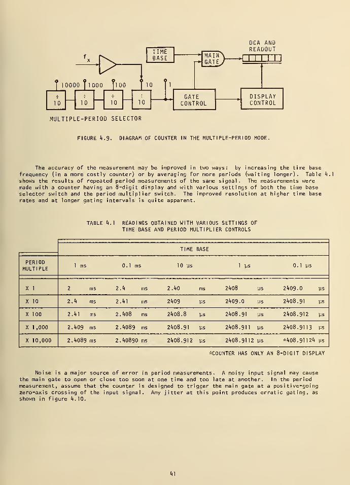
DCA AND
TIMEBASE
READOUTf •^ MA I
GAT" 1 *1
1 1 1 1 IX ^s^ y»>
1 10000 fiooc
>—?100 10
>
1
1
1
10 10 10
i GATE DISPLAY10 CONTROL CONTROL
MULTIPLE-PERIOD SELECTOR
FIGURE 4.9. DIAGRAM OF COUNTER IN THE MULTIPLE-PERIOD MODE.
The accuracy of the measurement may be improved in two ways: by increasing the time base
frequency (in a more costly counter) or by averaging for more periods (waiting longer). Tableshows the results of repeated period measurements of the same signal. The measurements weremade with a counter having an 8-digit display and with various settings of both the time base
selector switch and the period multiplier switch. The improved resolution at higher time base
rates and at longer gating intervals is quite apparent.
4.1
TABLE 4.1 READINGS OBTAINED WITH VARIOUS SETTINGS OFTIME BASE AND PERIOD MULTIPLIER CONTROLS
TIME BASE
PERIODMULTIPLE
1 ms 0.1 ms 10 ys 1 ys 0.1 ys
X 1 2 ms 2.4 ms 2.40 ms 2408 ys 2409.0 ys
X 10 2.4 ms 2.41 ms 2409 ys 2409.0 ys 2408.91 ys
X 100 2.41 ms 2.408 ms 2408.8 ys 2408.91 ys 2408.912 ys
X 1 ,000 2.409 ms 2.4089 ms 2408.91 ys 2408.911 ys 2408.9113 ys
X 10,000 2.4089 ms 2.40890 ms 2408.912 ys 2408.9112 ys *408.91124 ys
^COUNTER HAS ONLY AN 8-DIGIT DISPLAY
Noise is a major source of error in period measurements. A noisy input signal may causethe main gate to open or close too soon at one time and too late at another. In the periodmeasurement, assume that the counter is designed to trigger the main gate at a positive-goingzero-axis crossing of the input signal. Any jitter at this point produces erratic gating, as
shown i n figure 4.10.
41
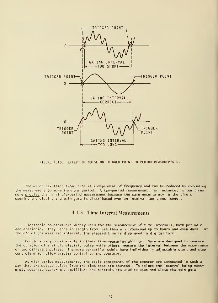
TRIGGER POINT-
TRIGGER POINT-
TRIGGER^POINT
GATING INTERVAL-. TOO SHORT +
GATING INTERVAL«. CORRECT +
-TRIGGER POINT
GATING INTERVALTOO LONG
TRIGGERPOINT
FIGURE *4.10. EFFECT OF NOISE ON TRIGGER POINT IN PERIOD MEASUREMENTS.
The error resulting from noise is independent of frequency and may be reduced by extendingthe measurement to more than one period. A ten-period measurement, for instance, is ten times
more preci se than a single-period measurement because the same uncertainty in the time of
opening and closing the main gate is distributed over an interval ten times longer.
4.1.3 Time Interval Measurements
Electronic counters are widely used for the measurement of time intervals, both periodicand aperiodic. They range in length from less than a microsecond up to hours and even days. Atthe end of the measured interval, the elapsed time is displayed in digital form.
Counters vary considerably in their time-measuring ability. Some are designed to measurethe duration of a single electric pulse while others measure the interval between the occurrenceof two different pulses. The more versatile models have individually adjustable start and stopcontrols which allow greater control by the operator.
As with period measurements, the basic components of the counter are connected in such a
way that the output pulses from the time base are counted. To select the interval being meas-ured, separate start-stop amplifiers and controls are used to open and close the main gate.
kl
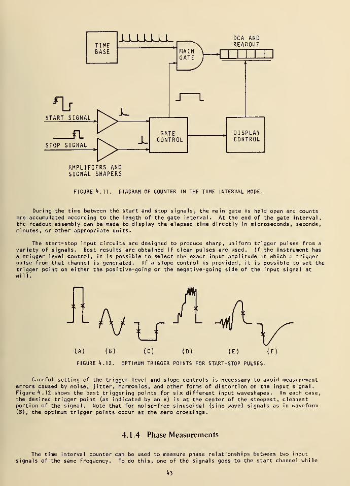
JJja_LLL
*bSTART SIGNAL
SISTOP SIGNAL
J^
DCA ANDREADOUT
J L
GATECONTROL
DISPLAYCONTROL
AMPLIFIERS ANDSIGNAL SHAPERS
FIGURE k.]]. DIAGRAM OF COUNTER IN THE TIME INTERVAL MODE.
During the time between the start and stop signals, the main gate is held open and countsare accumulated according to the length of the gate interval. At the end of the gate interval,the readout assembly can be made to display the elapsed time directly in microseconds, seconds,minutes, or other appropriate units.
The start-stop input circuits are designed to produce sharp, uniform trigger pulses from a
variety of signals. Best results are obtained if clean pulses are used. If the instrument has
a trigger level control, it is possible to select the exact input amplitude at which a triggerpulse from that channel is generated. If a slope control is provided, it is possible to set thetrigger point on either the positive-going or the negative-going side of the input signal at
will.
k >:
(A) (B) (C) (D) (E) (I
FIGURE 4.12. OPTIMUM TRIGGER POINTS FOR START-STOP PULSES.
Careful setting of the trigger level and slope controls is necessary to avoid measurementerrors caused by noise, jitter, harmonics, and other forms of distortion on the input signal.Figure 4.12 shows the best triggering points for six different input waveshapes. In each case,the desired trigger point (as indicated by an x) is at the center of the steepest, cleanestportion of the signal. Note that for noise-free sinusoidal (sine wave) signals as in waveform(B), the optimum trigger points occur at the zero crossings.
4.1.4 Phase Measurements
The time interval counter can be used to measure phase relationships between two input
signals of the same frequency. To do this, one of the signals goes to the start channel while
43
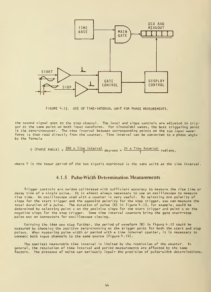
START
*^T GATECONTROL
OCA ANDREADOUT
DISPLAYCONTROL
FIGURE ^.13. USE OF T IME- I NTERVAL UNIT FOR PHASE MEASUREMENTS.
the second signal goes to the stop channel. The level and slope controls are adjusted to trig-ger at the same point on both input waveforms. For sinusoidal waves, the best triggering pointis the zero-crossover. The time interval between corresponding points on the two input wave-forms is then read directly from the counter. Time interval can be converted to a phase angleby the formula
[PHASE ANGLE) = 360 x Time Intervaldegrees = 2v x Time Interval
rad ians
,
where T is the known period of the two signals expressed in the same units as the time interval
4.1.5 Pulse-Width Determination Measurements
Trigger controls are seldom calibrated with sufficient accuracy to measure the rise time ordecay time of a single pulse. It is almost always necessary to use an oscilloscope to measurerise time. An oscilloscope used with a counter is very useful. By selecting one polarity of
slope for the start trigger and the opposite polarity for the stop trigger, you can measure the
total duration of a pulse. The duration of pulse (A) in figure ^.12, for example, could be
determined by selecting point x on the positive slope for the start trigger and point x on the
negative slope for the stop trigger. Some time interval counters bring the gate start-stoppulse out on connectors for oscilloscope viewing.
Carrying the idea one step further, the period of waveform (B) in figured. 12 could be
measured by choosing the positive zero-crossing as the trigger point for both the start and stoppulses. When measuring pulse width or period with a time interval counter, it is necessary to
connect both input channels to the same source (f igure *• . 1*0 .
The smallest measurable time interval is limited by the resolution of the counter. In
general, the resolution of time interval and period measurements are affected by the same
factors. The presence of noise can seriously impair the precision of pulse-width determinations.
kk
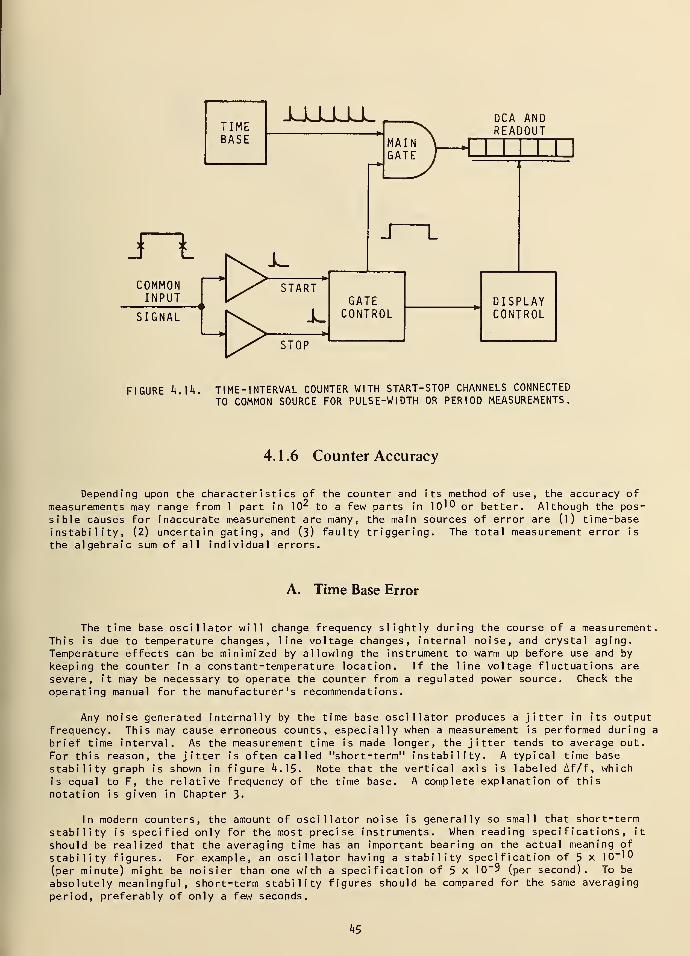
J~~LCOMMONINPUT
SIGNAL
JJJJJO-
STOP
DCA ANDREADOUT
J L
GATECONTROL
DISPLAYCONTROL
FIGURE k.]k. TIME-INTERVAL COUNTER WITH START-STOP CHANNELS CONNECTED
TO COMMON SOURCE FOR PULSE-WIDTH OR PERIOD MEASUREMENTS.
4. 1 .6 Counter Accuracy
Depending upon the characteristics of the counter and its method of use, the accuracy ofmeasurements may range from 1 part in 10^ to a few parts in 10^0 or better. Although the pos-sible causes for inaccurate measurement are many, the main sources of error are (1) time-baseinstability, (2) uncertain gating, and (3) faulty triggering. The total measurement error is
the algebraic sum of all individual errors.
A. Time Base Error
The time base oscillator will change frequency slightly during the course of a measurement.
This is due to temperature changes, line voltage changes, internal noise, and crystal aging.Temperature effects can be minimized by allowing the instrument to warm up before use and by
keeping the counter in a constant-temperature location. If the line voltage fluctuations aresevere, it may be necessary to operate the counter from a regulated power source. Check the
operating manual for the manufacturer's recommendations.
Any noise generated internally by the time base oscillator produces a jitter in its outputfrequency. This may cause erroneous counts, especially when a measurement is performed during a
brief time interval. As the measurement time is made longer, the jitter tends to average out.
For this reason, the jitter is often called "short-term" instability. A typical time base
stability graph is shown in figure 4.15. Note that the vertical axis is labeled Af/f, whichis equal to F, the relative frequency of the time base. A complete explanation of this
notation is given in Chapter 3.
In modern counters, the amount of oscillator noise is generally so small that short-term
stability is specified only for the most precise instruments. When reading specifications, it
should be realized that the averaging time has an important bearing on the actual meaning of
stability figures. For example, an oscillator having a stability specification of 5 x 10~'0
(per minute) might be noisier than one with a specification of 5 x 10"° (per second). To be
absolutely meaningful, short-term stability figures should be compared for the same averaging
period, preferably of only a few seconds.
h5
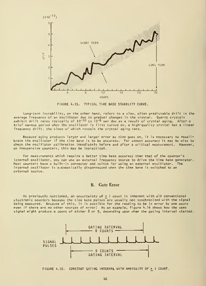
(X10~10
)
LONG TERM
FIGURE if. 15. TYPICAL TIME BASE STABILITY CURVE.
Long-term instability, on the other hand, refers to a slow, often predictable drift in the
average frequency of an oscillator due to gradual changes in the crystal. Quartz crystalsexhibit drift rates typically of 10"'° to 10"° per day as a result of crystal aging. After a
brief warmup period when the oscillator is first turned on, a high-quality crystal has a linear
frequency drift, the slope of which reveals the crystal aging rate.
Because aging produces larger and larger error as time goes on, it is necessary to recali-brate the oscillator if the time base is to be accurate. For utmost accuracy it may be wise to
check the oscillator calibration immediately before and after a critical measurement. However,on inexpensive counters, this may be impractical.
For measurements which require a better time base accuracy than that of the counter'sinternal oscillator, you can use an external frequency source to drive the time base generator.Most counters have a built-in connector and switch for using an external oscillator. Theinternal oscillator is automatically disconnected when the time base is switched to an
external source.
B. Gate Error
As previously mentioned, an uncertainty of + 1 count is inherent with all conventionalelectronic counters because the time base pulses are usually not synchronized with the signal
being measured. Because of this, it is possible for the reading to be in error by one counteven if there are no other sources of error! As an example, figure 4.16 shows how the same
signal might produce a count of either 8 or 9, depending upon when the gating interval started.
GATING INTERVAL8 COUNTS
PULSES
9 COUNTSGATING INTERVAL
IGNAL J r I k V * V l« l« Is ^-
FIGURE 4.16. CONSTANT GATING INTERVAL WITH AMBIGUITY OF + 1 COUNT.
46
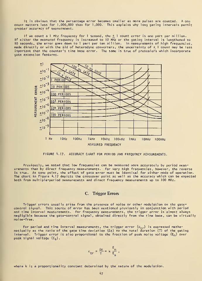
It is obvious that the percentage error becomes smaller as more pulses are counted. A onecount matters less for 1,000,000 than for 1,000. This explains why long gating intervals permitgreater accuracy of measurement.
If we count a 1 MHz frequency for 1 second, the + 1 count error is one part per million.If either the measured frequency is increased to 10 MHz or the gating interval is lengthened to
10 seconds, the error goes down to 1 part per ten million. In measurements of high frequencies,made directly or with the aid of heterodyne converters, the uncertainty of + 1 count may be less
important than the counter's time base error. The same is true of prescalers which incorporategate extension features.
+ 1
+ 10-1
+ 10
+ 10-3
DC +10
+ 10
°? +10 Tk
+ 10"
+ 10"
-7
^\; r^0 l^%- ^zisw
1 PERIOD*^! V,
10 PERIODS1
100 PERIODS1
103 PERIODS1
10*» PERIODS ^\1
105 PERIODS
1 Hz 10Hz 100Hz 1kHz 10kHz 100kHz
MEASURED FREQUENCY
1MHz 10MHz lOOMHi
FIGURE 4.17. ACCURACY CHART FOR PERIOD AND FREQUENCY MEASUREMENTS.
Previously, we noted that low frequencies can be measured more accurately by period meas-urements than by direct frequency measurements. For very high frequencies, however, the reverseis true. At some point, the effect of gate error must be identical for either mode of operation.The chart in figure 4.17 depicts the crossover point as well as the accuracy which can be expectedboth from multiple-period measurements and direct frequency measurements up to 100 MHz.
C. Trigger Errors
Trigger errors usually arise from the presence of noise or other modulation on the gate-control signal. This source of error has been mentioned previously in conjunction with periodand time interval measurements. For frequency measurements, the trigger error is almost alwaysnegligible because the gate-control signal, obtained directly from the time base, can be virtuallynoi se-f ree.
For period and time interval measurements, the trigger error (e«-r ) is expressed mathe-
matically as the ratio of the gate time deviation (At) to the total duration (T) of the gatinginterval. Trigger error is also proportional to the fraction of peak noise voltage (E n ) overpeak signal voltage (E s ).
tr
At , r
T =k T
where k is a proportionality constant determined by the nature of the modulation.
hi
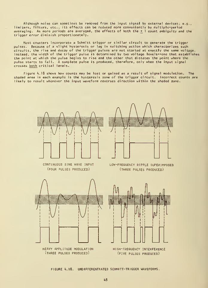
Although noise can sometimes be removed from the input signal by external devices; e.g.,limiters, filters, etc., its effects can be reduced more conveniently by multiple-periodaveraging. As more periods are averaged, the effects of both the + 1 count ambiguity and the
trigger error diminish proportionately.
Most counters incorporate a Schmitt trigger or similar circuit to generate the triggerpulses. Because of a slight hysteresis or lag in switching action which characterizes such
circuits, the rise and decay of the trigger pulses are not started at exactly the same voltage.Instead, the width of the trigger pulse is determined by two voltage levels—one that establishesthe point at which the pulse begins to rise and the other that dictates the point where the
pulse starts to fall. A complete pulse is produced, therefore, only when the input signal
crosses both critical levels.
Figure *4.l8 shows how counts may be lost or gained as a result of signal modulation. The
shaded area in each example is the hysteresis zone of the trigger circuit. Incorrect counts arelikely to result whenever the input waveform reverses direction within the shaded zone.
CONTINUOUS SINE WAVE INPUT
(FOUR PULSES PRODUCED)
LOW-FREQUENCY RIPPLE SUPERIMPOSED
(THREE PULSES PRODUCED)
HEAVY AMPLITUDE MODULATION(THREE PULSES PRODUCED)
HIGH-FREQUENCY INTERFERENCE
(FIVE PULSES PRODUCED)
FIGURE ^4. 18- UNDIFFERENTIATED SCHMITT-TR I GGER WAVEFORMS.
J»8
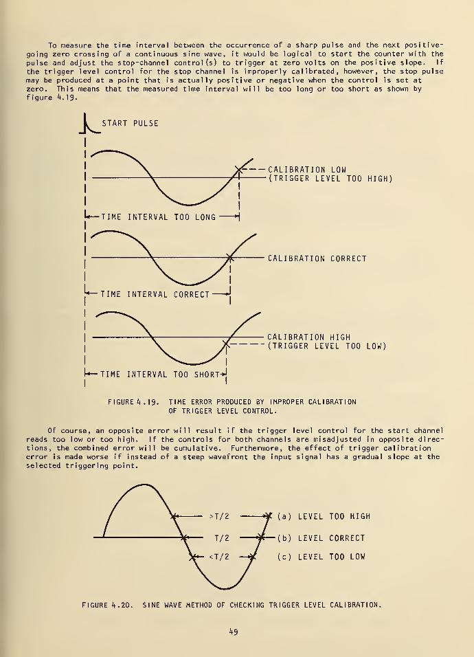
To measure the time interval between the occurrence of a sharp pulse and the next positive-
going zero crossing of a continuous sine wave, it would be logical to start the counter with the
pulse and adjust the stop-channel control (s) to trigger at zero volts on the positive slope. If
the trigger level control for the stop channel is improperly calibrated, however, the stop pulse
may be produced at a point that is actually positive or negative when the control is set atzero. This means that the measured time interval will be too long or too short as shown by
figure k. 19.
START PULSE
CALIBRATION LOW(TRIGGER LEVEL TOO HIGH)
CALIBRATION CORRECT
CALIBRATION HIGH(TRIGGER LEVEL TOO LOW)
TIME INTERVAL TOO SHORT-*!
FIGURE 4.19- TIME ERROR PRODUCED BY IMPROPER CALIBRATIONOF TRIGGER LEVEL CONTROL.
Of course, an opposite error will result if the trigger level control for the start channelreads too low or too high. If the controls for both channels are misadjusted in opposite direc-tions, the combined error will be cumulative. Furthermore, the effect of trigger calibrationerror is made worse if instead of a steep wavefront the input signal has a gradual slope at the
selected triggering point.
(a) LEVEL TOO HIGH
(b) LEVEL CORRECT
(c) LEVEL TOO LOW
FIGURE it. 20. SINE WAVE METHOD OF CHECKING TRIGGER LEVEL CALIBRATION.
hS
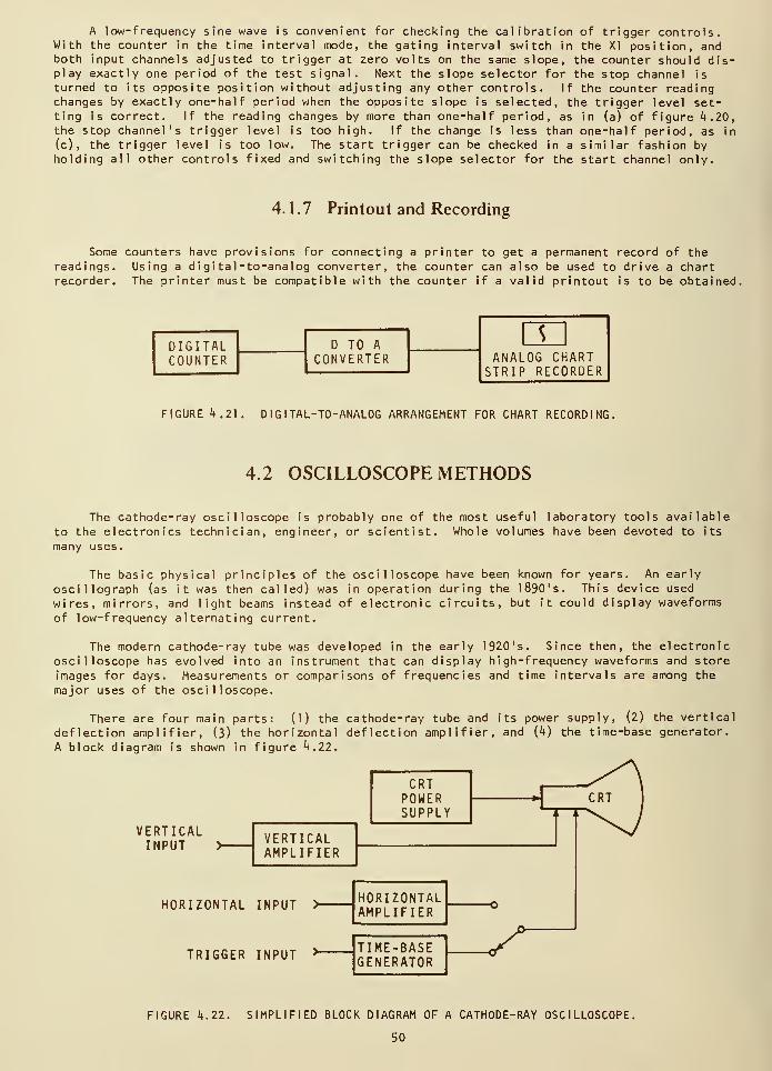
A low-frequency sine wave is convenienWith the counter in the time interval mode,both input channels adjusted to trigger atplay exactly one period of the test signal,turned to its opposite position without adj
changes by exactly one-half period when the
ting is correct. If the reading changes by
the stop channel's trigger level is too hig
(c) , the trigger level is too low. The sta
holding all other controls fixed and switch
t for checking the calibration of trigger controls,the gating interval switch in the XI position, and
zero volts on the same slope, the counter should dis-Next the slope selector for the stop channel is
usting any other controls. If the counter readingopposite slope is selected, the trigger level set-more than one-half period, as in (a) of figure 4.20,
h. If the change is less than one-half period, as in
rt trigger can be checked in a similar fashion by
ing the slope selector for the start channel only.
4.1.7 Printout and Recording
Some counters have provisions for connecting a printer to get a permanent record of the
readings. Using a digital-to-analog converter, the counter can also be used to drive a chartrecorder. The printer must be compatible with the counter if a valid printout is to be obtained.
sDIGITALCOUNTER
D TO A
CONVERTER ANALOG CHARTcTRTD crrnpnPR
FIGURE 4.21. DIGITAL-TO-ANALOG ARRANGEMENT FOR CHART RECORDING,
4.2 OSCILLOSCOPE METHODS
The cathode-ray oscilloscope is probably one of the most useful laboratory tools available
to the electronics technician, engineer, or scientist. Whole volumes have been devoted to its
many uses.
The basic physical principles of the oscilloscope have been known for years. An early
oscillograph (as it was then called) was in operation during the 1890's. This device used
wires, mirrors, and light beams instead of electronic circuits, but it could display waveforms
of low-frequency alternating current.
The modern cathode-ray tube was developed in the early 1920's. Since then, the electronicoscilloscope has evolved into an instrument that can display high-frequency waveforms and store
images for days. Measurements or comparisons of frequencies and time intervals are among the
major uses of the oscilloscope.
There are four main parts: (1) the cathode-ray tube and its power supply, (2) the vertical
deflection amplifier, (3) the horizontal deflection amplifier, and (4) the time-base generator.
A block diagram is shown in figure 4.22.
VERTICALINPUT
VERTICALAMPLIFIER
CRTPOWERSUPPLY T~T
HORIZONTAL INPUT >-HORIZONTALAMPLIFIER
TRIGGER INPUT >" TIME-BASEGENERATOR
SFIGURE 4.22. SIMPLIFIED BLOCK DIAGRAM OF A CATHODE-RAY OSCILLOSCOPE.
50
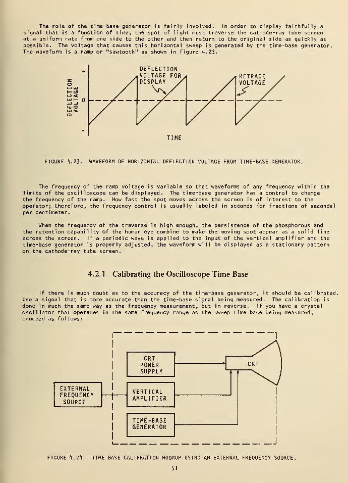
The role of the time-base generator is fairly involved. In order to display faithfully a
signal that is a function of time, the spot of light must traverse the cathode-ray tube screenat a uniform rate from one side to the other and then return to the original side as quickly as
possible. The voltage that causes this horizontal sweep is generated by the time-base generator,The waveform is a ramp or "sawtooth" as shown in figure 4.23.
DEFLECTIONVOLTAGE FOR
TIME
FIGURE 4.23. WAVEFORM OF HORIZONTAL DEFLECTION VOLTAGE FROM TIME-BASE GENERATOR.
The frequency of the ramp voltage is variable so that waveforms of any frequency within thelimits of the oscilloscope can be displayed. The time-base generator has a control to changethe frequency of the ramp. How fast the spot moves across the screen is of interest to theoperator; therefore, the frequency control is usually labeled in seconds (or fractions of seconds)per centimeter.
When the frequency of the traverse is high enough, the persistence of the phosphorous andthe retention capability of the human eye combine to make the moving spot appear as a solid line
across the screen. If a periodic wave is applied to the input of the vertical amplifier and the
time-base generator is properly adjusted, the waveform will be displayed as a stationary patternon the cathode-ray tube screen.
4.2. 1 Calibrating the Oscilloscope Time Base
If there is much doubt as to the accuracy of the time-base generator, it should be calibratedUse a signal that is more accurate than the time-base signal being measured. The calibration is
done in much the same way as the frequency measurement, but in reverse. If you have a crystaloscillator that operates in the same frequency range as the sweep time base being measured,proceed as follows:
EXTERNALFREQUENCYSOURCE
CRTPOWERSUPPLY
VERTICALAMPLIFIER
TIME-BASEGENERATOR
FIGURE h.lk. TIME BASE CALIBRATION HOOKUP USING AN EXTERNAL FREQUENCY SOURCE.
51
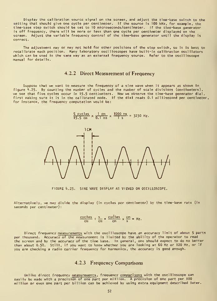
Display the calibration source signal on the screen, and adjust the time-base switch to thesetting that should give one cycle per centimeter. If the source is 100 kHz, for example, thetime-base step switch should be set to 10 microseconds/centimeter. If the time-base generatoris off frequency, there will be more or less than one cycle per centimeter displayed on thescreen. Adjust the variable frequency control of the time-base generator until the display is
correct.
The adjustment may or may not hold for other positions of the step switch, so it is best to
recalibrate each position. Many laboratory oscilloscopes have built-in calibration oscillatorswhich can be used in the same way as an external frequency source. Refer to the oscilloscopemanual for details.
4.2.2 Direct Measurement of Frequency
Suppose that we want to measure the frequency of a sine wave when it appears as shown in
figure ^.25. By counting the number of cycles and the number of scale divisions (centimeters),we see that five cycles occur in 15.5 centimeters. Now we observe the time-base generator dial,
first making sure it is in the calibrated mode. If the dial reads 0.1 millisecond per centimeter,for instance, the frequency computation would be:
5 cycles 1! v
15-5 cm 0. 1 ms
1000 ms
1 s3230 Hz.
FIGURE 4.25. SINE WAVE DISPLAY AS VIEWED ON OSCILLOSCOPE.
Alternatively, we may divide the display (in cycles per centimeter) by the time-base rate (in
seconds per centimeter):
cycles . s cycles cm u—'- f — = —
'
x — = Hz.
Direct frequency measurements with the oscilloscope have an accuracy limit of about 5 parts
per thousand. Accuracy of the measurement is limited by the ability of the operator to read
the screen and by the accuracy of the time base. In general, one should expect to do no better
than about 0.5%. Still, if you want to know whether you are looking at 60 Hz or 120 Hz, or if
you are checking a radio carrier frequency for harmonics, the accuracy is good enough.
4.2.3 Frequency Comparisons
Unlike direct frequency measurements , frequency comparisons with the oscilloscope can
easily be made with a precision of one part per million. A precision of one part per 100
million or even one part per billion can be achieved by using extra equipment described later.
52
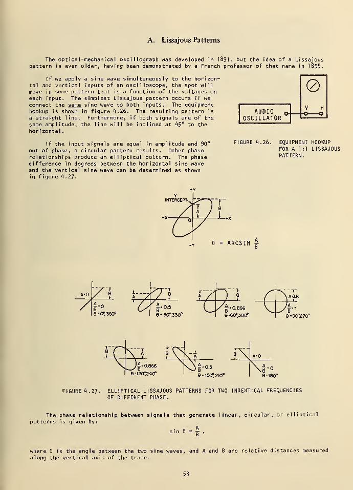
A. Lissajous Patterns
The optical -mechanical oscillograph was developed in 1891, but the idea of a Lissajouspattern is even older, having been demonstrated by a French professor of that name in 1855-
If we apply a sine wave simultaneously to the horizon-tal and vertical inputs of an oscilloscope, the spot willmove in some pattern that is a function of the voltages on
each input. The simplest Lissajous pattern occurs if weconnect the same sine wave to both inputs. The equipmenthookup is shown in figure if. 26. The resulting pattern is
a straight line. Furthermore, if both signals are of the
same amplitude, the line will be inclined at 45° to the
horizontal
.
If the input signals are equal in amplitude and 90°
out of phase, a circular pattern results. Other phaserelationships produce an elliptical pattern. The phasedifference in degrees between the horizontal sine waveand the vertical sine wave can be determined as shownin figure 4.27.
V HAUDIO o.
OSCILLATOR
FIGURE 4.26. EQUIPMENT HOOKUP
FOR A 1:1 LISSAJOUSPATTERN.
= ARCSINJ.
9«0°,360° 9 30°,330° 9 =90°,270°
0.866
e = 120°,240° 9=150,210° 9 = 180°
FIGURE 4.27. ELLIPTICAL LISSAJOUS PATTERNS FOR TWO INDENTICAL FREQUENCIES
OF DIFFERENT PHASE.
The phase relationship between signals that generate linear, circular, or elliptical
patterns is given by:
. . Asin 6 = j ,
where is the angle between the two sine waves, and A and B are relative distances measured
along the vertical axis of the trace.
53
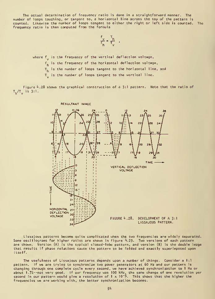
The actual determination of frequency ratio is done in a straightforward manner. The
number of loops touching, or tangent to, a horizontal line across the top of the pattern is
counted. Likewise the number of loops tangent to either the right or left side is counted. Thefrequency ratio is then computed from the formula
where f is the frequency of the vertical deflection voltage,
f, is the frequency of the horizontal deflection voltage,h
T, is the number of loops tangent to the horizontal line, andn
T is the number of loops tangent to the vertical line,v
Figure ^.28 shows the graphical construction of a 3:1 pattern. Note that the ratio of
T./T is 3=1n v
RESULTANT IMAGE
0-36 24
HORIZONTAL 27DEFLECTIONVOLTAGE
33 FIGURE k .28. DEVELOPMENT OF A 3:1
LISSAJOUS PATTERN.
Lissajous patterns become quite complicated when the two frequencies are widely separated.Some oscillograms for higher ratios are shown in figure ^.29. Two versions of each patternare shown. Version (A) is the typical closed-lobe pattern, and version (B) is the double image
that results if phase relations cause the pattern to be folded and exactly superimposed uponitself.
The usefulness of Lissajous patterns depends upon a number of things. Consider a 1:1
pattern. If we are trying to synchronize two power generators at 60 Hz and our pattern is
changing through one complete cycle every second, we have achieved synchronization to 1 Hz or
about 1.7l __not very good. If our frequency was 100 kHz, the same change of one revolution per
second in our pattern would give a resolution of 1 x 10"5. This shows that the higher the
frequencies we are working with, the better synchronization becomes.
5k
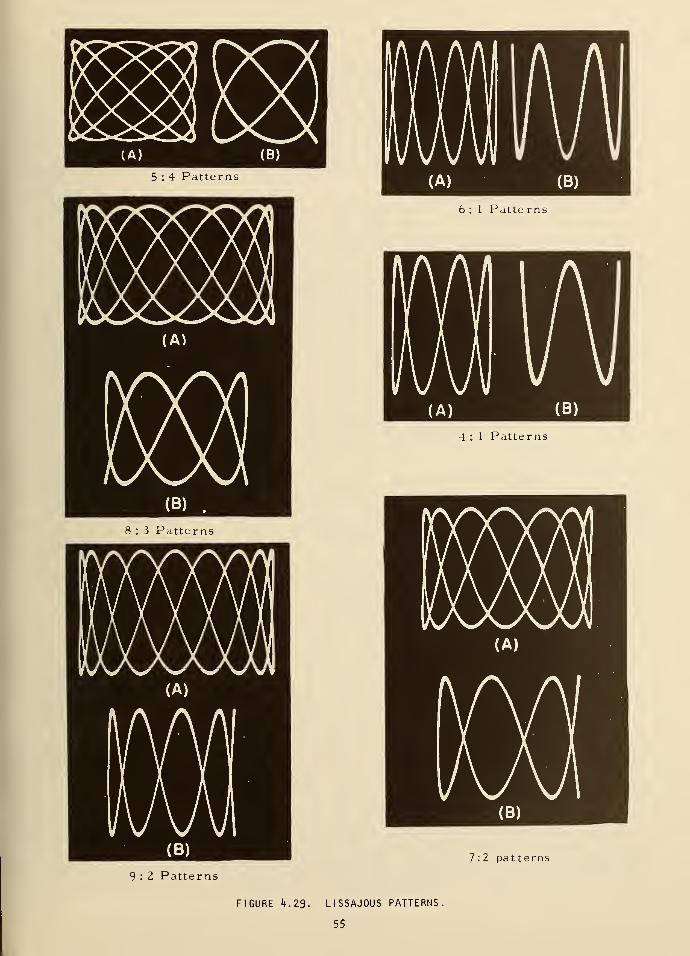
5 : 4 Patterns
6 : 1 Patte rns
4 : 1 Patterns
7:2 patterns
9 : 2 Patterns
FIGURE 4.29. LISSAJOUS PATTERNS,
55
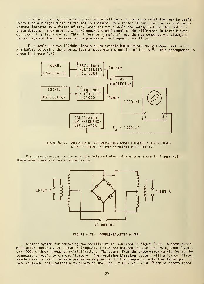
In comparing or synchronizing precision oscillators, a frequency multiplier may be useful.Every time our signals are multiplied in frequency by a factor of ten, the precision of meas-urement improves by a factor of ten. When the two signals are multiplied and then fed to a
phase detector, they produce a low-frequency signal equal to the difference in hertz betweenour two multiplied signals. This difference signal, Af. may then be compared via Lissajouspattern against the sine wave from a precision low-frequency oscillator.
If we again use two 100-kHz signals as an example but multiply their frequencies to 100MHz before comparing them, we achieve a measurement precision of 1 x 10"°. This arrangement is
shown in figure 4.30.
100kHz
OSCILLATOR
FREQUENCYMULTIPLIER(X1000)
100MHz
100kHz
OSCILLATOR
FREQUENCYMULTIPLIER(X1000)
•-* PHASE
r* DETECTOR
100MHz1000 AF
CALIBRATEDLOW FREQUENCYOSCILLATOR
©F„ = 1000 AF
FIGURE 4.30. ARRANGEMENT FOR MEASURING SMALL FREQUENCY DIFFERENCESWITH OSCILLOSCOPE AND FREQUENCY MULTIPLIERS.
The phase detector may be a double-balanced mixer of the type shown in figure 4.31
These mixers are available commercially.
INPUT INPUT B
DC OUTPUT
FIGURE 4.31. DOUBLE-BALANCED MIXER.
Another system for comparing two oscillators is indicated in figure 4.32. A phase-errormultiplier increases the phase or frequency difference between the oscillators by some factor,say 1000, without frequency multiplication. The output from the phase-error multiplier can be
connected directly to the oscilloscope. The resulting Lissajous pattern will al low osci 1 lator
synchronization with the same precision as provided by the frequency multiplier technique. If
care is taken, calibrations with errors as small as 1 x 10"9 or 1 x 10"10 can be accomplished.
56
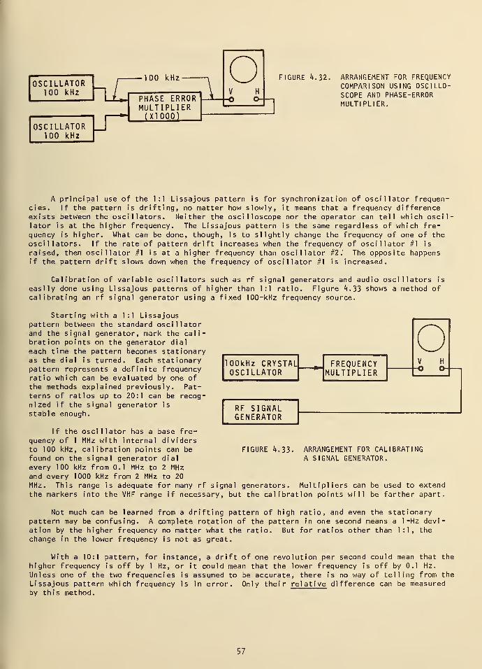
OSCILLATOR100 kHz hL
OSCILLATOR100 kHz
100 kHz
PHASE ERRORMULTIPLIER(X1000)
1o
E2
FIGURE 4. 32. ARRANGEMENT FOR FREQUENCYCOMPARISON USING OSCILLO-SCOPE AND PHASE-ERRORMULTIPLIER.
A principal use of the 1:1 Lissajous pattern is for synchronization of oscillator frequen-cies. If the pattern is drifting, no matter how slowly, it means that a frequency differenceexists between the oscillators. Neither the oscilloscope nor the operator can tell which oscillator is at the higher frequency. The Lissajous pattern is the same regardless of which fre-quency is higher. What can be done, though, is to slightly change the frequency of one of the
oscillators. If the rate of pattern drift increases when the frequency of oscillator #1 is
raised, then oscillator #1 is at a higher frequency than oscillator #2." The opposite happensif the pattern drift slows down when the frequency of oscillator #1 is increased.
Calibration of variable oscillators such as rf signal generators and audio oscillators is
easily done using Lissajous patterns of higher than 1:1 ratio. Figure 4.33 shows a method ofcalibrating an rf signal generator using a fixed 100-kHz frequency source.
Starting with a 1:1 Lissajouspattern between the standard oscillatorand the signal generator, mark the cali-bration points on the generator dial
each time the pattern becomes stationaryas the dial is turned. Each stationarypattern represents a definite frequencyratio which can be evaluated by one ofthe methods explained previously. Pat-terns of ratios up to 20:1 can be recog-nized if the signal generator is
stable enough.
100kHz CRYSTAL!OSCILLATOR
FREQUENCYMULTIPLIER
RF SIGNALGENERATOR
If the oscillator has a base fre-quency of 1 MHz with internal dividersto 100 kHz, calibration points can be FIGURE 4.33.found on the signal generator dial
every 100 kHz from 0.1 MHz to 2 MHzand every 1000 kHz from 2 MHz to 20
MHz. This range is adequate for many rf signal generators.
ARRANGEMENT FOR CALIBRATINGA SIGNAL GENERATOR.
Multipliers can be used to extendthe markers into the VHF range if necessary, but the calibration points will be farther apart.
Not much can be learned from a drifting pattern of high ratio, and even the stationarypattern may be confusing. A complete rotation of the pattern in one second means a 1 -Hz devi-ation by the higher frequency no matter what the ratio. But for ratios other than 1:1, the
change in the lower frequency is not as great.
With a 10:1 pattern, for instance, a drift of one revolution per second could mean that the
higher frequency is off by 1 Hz, or it could mean that the lower frequency is off by 0.1 Hz.
Unless one of the two frequencies is assumed to be accurate, there is no way of telling from the
Lissajous pattern which frequency is in error. Only their relative difference can be measuredby this method.
57
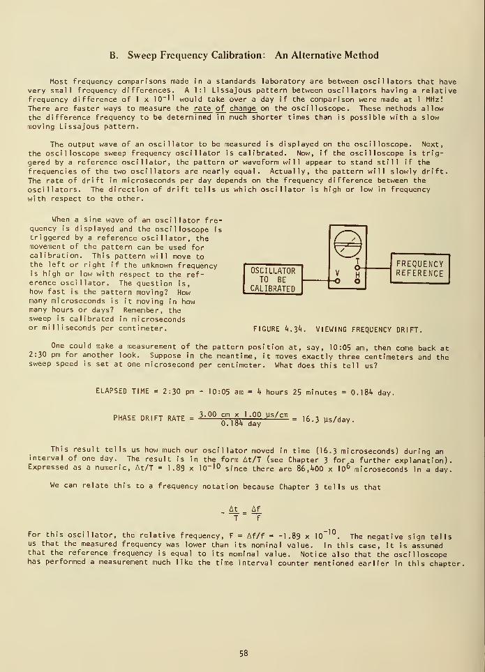
B. Sweep Frequency Calibration: An Alternative Method
Most frequency comparisons made in a standards laboratory are between oscillators that havevery small frequency differences. A 1:1 Lissajous pattern between oscillators having a relativefrequency difference of 1 x 10"!
1 would take over a day if the comparison were made at 1 MHz!
There are faster ways to measure the rate of change on the oscilloscope. These methods allowthe difference frequency to be determined in much shorter times than is possible with a slowmoving Lissajous pattern.
The output wave of an oscillator to be measured is displayed on the oscilloscope. Next,
the oscilloscope sweep frequency oscillator is calibrated. Now, if the oscilloscope is trig-gered by a reference oscillator, the pattern or waveform will appear to stand still if the
frequencies of the two oscillators are nearly equal. Actually, the pattern will slowly drift.
The rate of drift in microseconds per day depends on the frequency difference between the
oscillators. The direction of drift tells us which oscillator is high or low in frequencywith respect to the other.
When a sine wave of an oscillator fre-quency is displayed and the oscilloscope is
triggered by a reference oscillator, themovement of the pattern can be used forcalibration. This pattern will move tothe left or right if the unknown frequencyis high or low with respect to the ref-erence oscillator. The question is,how fast is the pattern moving? Howmany microseconds is it moving in howmany hours or days? Remember, thesweep is calibrated in microsecondsor milliseconds per centimeter. FIGURE h.},k. VIEWING FREQUENCY DRIFT.
One could make a measurement of the pattern position at, say, 10:05 am, then come back at2:30 pm for another look. Suppose in the meantime, it moves exactly three centimeters and thesweep speed is set at one microsecond per centimeter. What does this tell us?
ELAPSED TIME = 2:30 pm - 10:05 am = k hours 25 minutes = 0.184 day.
PHASE DRIFT RATE = 3 -°° ™^ -°° ys/cm= 16. 3 ys/day.
This result tells us how much our oscillator moved in time (16.3 microseconds) during aninterval of one day. The result is in the form At/T (see Chapter 3 for a further explanation).Expressed as a numeric, At/T = 1.89 x 10 -10 since there are 86,^00 x 10 6 microseconds in a day.
We can relate this to a frequency notation because Chapter 3 tells us that
OSCILLATORTO BE
CALIBRATED
FREQUENCYREFERENCE
A_t_
T
Aff
•10For this oscillator, the relative frequency, F = Af/f = -1.89 x 10" ,w. The negative sign tells
us that the measured frequency was lower than its nominal value. In this case, It is assumedthat the reference frequency is equal to its nominal value. Notice also that the oscilloscopehas performed a measurement much like the time interval counter mentioned earlier in this chapter.
58
4.2.4 Time Interval Measurements
Time-interval measurements are quite easy to perform with the oscilloscope. Usually, onetime pulse is displayed on the screen while a different time pulse is used to trigger the oscil-loscope. Another method is to display both time pulses on a dual-trace scope. Triggering can
be achieved from either of the two displayed pulses or from a third time pulse. An adjustable
rate divider is handy for this purpose.
A point worth remembering is that the accuracy of the time-interval measurement is inversely
proportional to the length of the interval. If the time pulses are 10 milliseconds apart, for
instance, the measurement can be performed to probably no better than +50 microseconds. But if
the pulses are only 100 microseconds apart, the measurement can be performed with an accuracy of
+_ 0.5 microsecond. In both cases, however, the relative uncertainty is the same (+_ 5 parts
in 103).
For time pulses spaced close together, the pulse width may occupy an appreciable percent of
the time interval; therefore, large errors can be introduced by having the wrong trigger slopeor improper trigger amplitude. Unless care is taken by the operator, such errors can nullifythe accuracy that is otherwise attainable in the measurement of brief time intervals.
The main advantage in using an oscilloscope for time interval measurements is that one can
see the pulse waveform. For this reason, time intervals between odd-shaped or noisy pulses arebetter measured with the oscilloscope than with other types of instruments. Time intervals in
the submicrosecond range can be measured easily and economically with high-frequency oscilloscopes,but long intervals are more accurately measured with an electronic counter, as described earlier.Always refer to your oscilloscope manual; it contains additional useful information.
4.3 WAVEMETERS
A wavemeter is an adjustable circuit that can be made to resonate over a range of frequenciesas indicated on a calibrated dial. The dial may be marked in units of frequency or wavelength.A typical wavemeter covers a frequency range on the order of one octave. Resonance is detectedby observing the response of a meter or other device incorporated into the measuring instrumentor by noting a disturbance in the system under test.
Wavemeters are sometimes classified as transmission types or as absorption types dependingon the way they are connected to the frequency source being checked. A transmission-type wave-meter has connectors at both input and output ends so it can be put into the circuit under test.An absorption-type (or reaction-type) meter, on the other hand, is designed for loose couplingvia the electromagnetic field of the frequency source.
The simplest LC absorption wavemeter for measuring radio frequencies consists of a coil anda variable capacitor in series. The capacitor shaft has a calibrated dial so the resonantfrequency of the LC circuit can be read off as the capacitor is adjusted.
The simple wavemeter is used by holding it near the frequency source being measured. It is
then tuned while watching for a sharp reaction by the source. The frequency is read from thecalibrated dial. The reaction is caused by the absorption of a small amount of rf energy fromthe source by the wavemeter when the two are at the same frequency. In measuring the frequencyof a small transmitter, one might look for a flicker in the power stage current as the wavemeteris tuned through resonance. Because of the loose coupling and the small power consumed by thewavemeter, the energy taken from high-power sources might go unnoticed; therefore, an indicatoris built into the wavemeter itself.
59
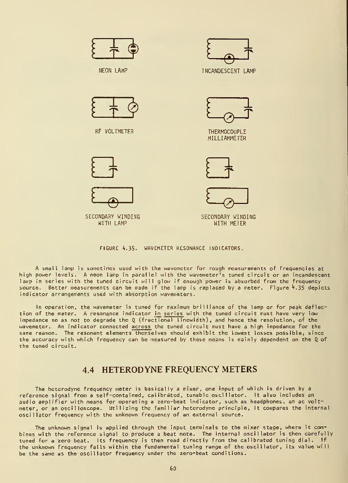
raNEON LAMP
1
INCANDESCENT LAMP
ORF VOLTMETER THERMOCOUPLE
MILLIAMMETER
J*
"1
T
e-SECONDARY WINDING
WITH LAMPSECONDARY WINDING
WITH METER
FIGURE 4.35. WAVEMETER RESONANCE INDICATORS.
A small lamp is sometimes used with the wavemeter for rough measurements of frequencies at
high power levels. A neon lamp in parallel with the wavemeter's tuned circuit or an incandescentlamp in series with the tuned circuit will glow if enough power is absorbed from the frequencysource. Better measurements can be made if the lamp is replaced by a meter. Figure ^.35 depictsindicator arrangements used with absorption wavemeters.
In operation, the wavemeter is tuned for maximum brilliance of the lamp or for peak deflec-tion of the meter. A resonance indicator in series with the tuned circuit must have very low
impedance so as not to degrade the Q. (fractional linewidth), and hence the resolution, of the
wavemeter. An indicator connected across the tuned circuit must have a high impedance for the
same reason. The resonant elements themselves should exhibit the lowest losses possible, sincethe accuracy with which frequency can be measured by these means is mainly dependent on the Q. of
the tuned circuit.
4.4 HETERODYNE FREQUENCY METERS
The heterodyne frequency meter is basically a mixer, one input of which is driven by a
reference signal from a self-contained, calibrated, tunable oscillator. It also includes an
audio amplifier with means for operating a zero-beat indicator, such as headphones, an ac volt-
meter, or an oscilloscope. Utilizing the familiar heterodyne principle, it compares the internal
oscillator frequency with the unknown frequency of an external source.
The unknown signal is applied through the input terminals to the mixer stage, where it com-
bines with the reference signal to produce a beat note. The internal oscillator is then carefully
tuned for a zero beat. Its frequency is then read directly from the calibrated tuning dial. If
the unknown frequency falls within the fundamental tuning range of the oscillator, its value will
be the same as the oscillator frequency under the zero-beat conditions.
60
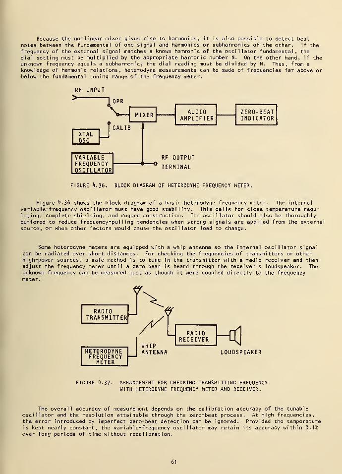
Because the nonlinear mixer gives rise to harmonics, it is also possible to detect beatnotes between the fundamental of one signal and harmonics or subharmonics of the other. If the
frequency of the external signal matches a known harmonic of the oscillator fundamental, the
dial setting must be multiplied by the appropriate harmonic number N. On the other hand, if theunknown frequency equals a subharmonic, the dial reading must be divided by N. Thus, from a
knowledge of harmonic relations, heterodyne measurements can be made of frequencies far above orbelow the fundamental tuning range of the frequency meter.
RF INPUT
Topr
XTALOSCJ
MIXER
CALIB
VARIABLEFREQUENCYOSCILLATOR
AUDIOAMPLIFIER
ZERO-BEATINDICATOR
RF OUTPUT
TERMINAL
FIGURE 4. 36. BLOCK DIAGRAM OF HETERODYNE FREQUENCY METER.
Figure 4.36 shows the block diagram of a basic heterodyne frequency meter. The internal
variable-frequency oscillator must have good stability. This calls for close temperature regu-
lation, complete shielding, and rugged construction. The oscillator should also be thoroughlybuffered to reduce frequency-pulling tendencies when strong signals are applied from the externalsource, or when other factors would cause the oscillator load to change.
Some heterodyne meters are equipped with a whip antenna so the internal oscillator signalcan be radiated over short distances. For checking the frequencies of transmitters or otherhigh-power sources, a safe method is to tune in the transmitter with a radio receiver and thenadjust the frequency meter until a zero beat is heard through the receiver's loudspeaker. Theunknown frequency can be measured just as though it were coupled directly to the frequencymeter.
VRADIO
TRANSMITTERJ <y
HETERODYNEFREQUENCY
METER
WHIPANTENNA
RADIORECEIVER w
LOUDSPEAKER
FIGURE 4.37. ARRANGEMENT FOR CHECKING TRANSMITTING FREQUENCYWITH HETERODYNE FREQUENCY METER AND RECEIVER.
The overall accuracy of measurement depends on the calibration accuracy of the tunableoscillator and the resolution attainable through the zero-beat process. At high frequencies,the error introduced by imperfect zero-beat detection can be ignored. Provided the temperatureis kept nearly constant, the variable-frequency oscillator may retain its accuracy within 0.1%over long periods of time without recal ibrat ion.
61
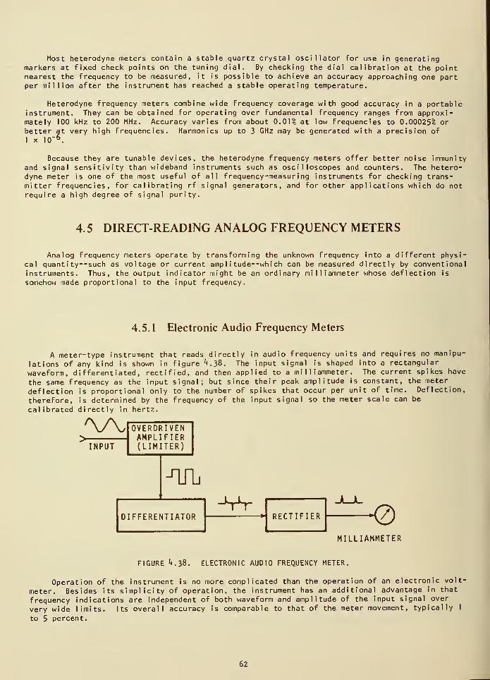
Most heterodyne meters contain a stable quartz crystal oscillator for use in generatingmarkers at fixed check points on the tuning dial. By checking the dial calibration at the pointnearest the frequency to be measured, it is possible to achieve an accuracy approaching one partper million after the instrument has reached a stable operating temperature.
Heterodyne frequency meters combine wide frequency coverage with good accuracy in a portableinstrument. They can be obtained for operating over fundamental frequency ranges from approxi-mately 100 kHz to 200 MHz. Accuracy varies from about 0.01 % at low frequencies to 0.00025% or
better at very high frequencies. Harmonics up to 3 GHz may be generated with a precision of
1 x 10~ 6.
Because they are tunable devices, the heterodyne frequency meters offer better noise immunityand signal sensitivity than wideband instruments such as oscilloscopes and counters. The hetero-dyne meter is one of the most useful of all frequency-measuring instruments for checking trans-mitter frequencies, for calibrating rf signal generators, and for other applications which do notrequire a high degree of signal purity.
4.5 DIRECT-READING ANALOG FREQUENCY METERS
Analog frequency meters operate by transforming the unknown frequency into a different physi-cal quant i ty--such as voltage or current ampl i tude--which can be measured directly by conventionalinstruments. Thus, the output indicator might be an ordinary milliammeter whose deflection is
somehow made proportional to the input frequency.
4.5.1 Electronic Audio Frequency Meters
A meter-type instrument that reads directly in audio frequency units and requires no manipu-
lations of any kind is shown in figure ^.38. The input signal is shaped into a rectangular
waveform, differentiated, rectified, and then applied to a milliammeter. The current spikes have
the same frequency as the input signal; but since their peak amplitude is constant, the meter
deflection is proportional only to the number of spikes that occur per unit of time. Deflection,
therefore, is determined by the frequency of the input signal so the meter scale can be
calibrated directly in hertz.wINPUT
OVERDRIVENAMPLIFIER(LIMITER)
-TJL
DIFFERENTIATORVr
• RECTIFIER <2>MILLIAMMETER
FIGURE 4 . 38. ELECTRONIC AUDIO FREQUENCY METER.
Operation of the instrument is no more complicated than the operation of an electronic volt-
meter. Besides its simplicity of operation, the instrument has an additional advantage in that
frequency indications are independent of both waveform and amplitude of the input signal over
very wide limits. Its overall accuracy is comparable to that of the meter movement, typically 1
to 5 percent.
62
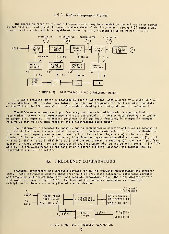
4.5.2 Radio Frequency Meters
The operating range of the audio frequency meter may be extended to the VHF region or higherby adding a series of decade frequency scalers ahead of the instrument. Figure 4 - 39 shows a dia-gram of such a device which is capable of measuring radio frequencies up to 50 MHz directly.
INPUT >
TUNING METER
"7TUNING METER TUNING METER TUNING METER
AUDIO •-vEQUENCY —(/)METER V^/
FIGURE 4.39- DIRECT-READING RADIO FREQUENCY METER.
The audio frequency meter is preceded by four mixer stages, each excited by a signal derivedfrom a standard 1 MHz crystal oscillator. The injection frequency for the first mixer consistsof the 25th to the 49th harmonic of 1 MHz as determined by the tuning of harmonic selector A.
The difference between the input frequency and the selected harmonic is then applied to a
second mixer, where it is heterodyned against a subharmonic of 1 MHz as determined by the tuningof harmonic selector B. The process continues until the input frequency is eventually reducedto a value that falls within range of the direct-reading audio meter.
The instrument is operated by manually tuning each harmonic selector and mixer in successionfor peak deflection on the associated tuning meter. Each harmonic selector dial is calibrated so
that the input frequency can be read directly from the dial settings in conjunction with the
reading of the audio meter. For example, if optimum tuning occurs when dial A is set at 32, dial
B is at 7, dial C is at 5, dial D is at 9, and the audio meter is reading 170, then the input fre-quency is 32.759170 MHz. Typical accuracy of the instrument with an analog audio meter is 5 x 10"'
at VHF. If the audio meter is replaced by an electronic digital counter, the accuracy may be
improved to 2 x 10"8 or better.
4.6 FREQUENCY COMPARATORS
Frequency comparators are versatile devices for making frequency measurements and compari-
sons. These instruments combine phase error multipliers, phase detectors, integrated circuitsand frequency multipliers into useful and accurate laboratory aids. The block diagram of this
instrument is shown in figure h.kO. The heart of the frequency comparator is a variable-multiplication phase error multiplier of special design.
TO CHARTrR
INPUT
FX
INPUT
RECOF
PHASE ERRORMULTIPLIER
XI1
TO XI4
FREQUENCYDISCRIMINATOR
DC VOLTMETERCALIBRATED IN
"PARTS IN 10 N "
i
F ni
PHASEDETECTOR
,J. C TO COUNTER, » nrcF
R+10 N
AFOSCILLOSCOPE1
FIGURE k.kO. BASIC FREQUENCY COMPARATOR.
63
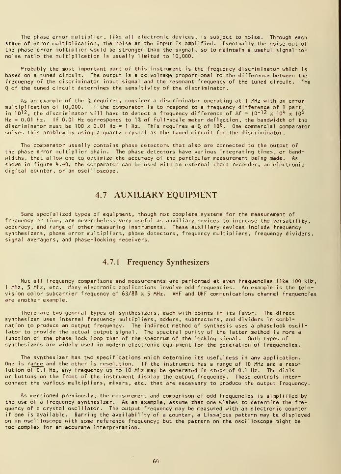
The phase error multiplier, like all electronic devices, is subject to noise. Through eachstage of error multiplication, the noise at the input is amplified. Eventually the noise out ofthe phase error multiplier would be stronger than the signal, so to maintain a useful signal-to-noise ratio the multiplication is usually limited to 10,000.
Probably the most important part of this instrument is the frequency discriminator which is
based on a tuned-circuit. The output is a dc voltage proportional to the difference between thefrequency of the discriminator input signal and the resonant frequency of the tuned circuit. The
Q of the tuned circuit determines the sensitivity of the discriminator.
As an example of the Q required, consider a discriminator operating at 1 MHz with an errormultiplication of 10,000. If the comparator is to respond to a frequency difference of 1 partin 10l2
;the discriminator will have to detect a frequency difference of Af = 10~'2 x lO'4 x 10°
Hz = 0.01 Hz. If 0.01 Hz corresponds to ]% of full-scale meter deflection, the bandwidth of thediscriminator must be 100 x 0.01 Hz = 1 Hz. This requires a Q of 10°. One commercial comparatorsolves this problem by using a quartz crystal as the tuned circuit for the discriminator.
The comparator usually contains phase detectors that also are connected to the output of
the phase error multiplier chain. The phase detectors have various integrating times, or band-widths, that allow one to optimize the accuracy of the particular measurement being made. As
shown in figure *4.40, the comparator can be used with an external chart recorder, an electronicdigital counter, or an oscilloscope.
4.7 AUXILIARY EQUIPMENT
Some specialized types of equipment, though not complete systems for the measurement offrequency or time, are nevertheless very useful as auxiliary devices to increase the versatility,accuracy, and range of other measuring instruments. These auxiliary devices include frequencysynthesizers, phase error multipliers, phase detectors, frequency multipliers, frequency dividers,signal averagers, and phase-locking receivers.
4.7.1 Frequency Synthesizers
Not all frequency comparisons and measurements are performed at even frequencies like 100 kHz,1 MHz, 5 MHz, etc. Many electronic applications involve odd frequencies. An example is the tele-vision color subcarrier frequency of 63/88 x 5 MHz. VHF and UHF communications channel frequenciesare another example.
There are two general types of synthesizers, each with points in its favor. The directsynthesizer uses internal frequency multipliers, adders, subtracters, and dividers in combi-nation to produce an output frequency. The indirect method of synthesis uses a phaselock oscil-lator to provide the actual output signal. The spectral purity of the latter method is more a
function of the phase-lock loop than of the spectrum of the locking signal. Both types ofsynthesizers are widely used in modern electronic equipment for the generation of frequencies.
The synthesizer has two specifications which determine its usefulness in any application.One is range and the other is resolution . If the instrument has a range of 10 MHz and a reso-lution of 0.1 Hz, any frequency up to 10 MHz may be generated in steps of 0.1 Hz. The dialsor buttons on the front of the instrument display the output frequency. These controls inter-connect the various multipliers, mixers, etc. that are necessary to produce the output frequency.
As mentioned previously, the measurement and comparison of odd frequencies is simplified by
the use of a frequency synthesizer. As an example, assume that one wishes to determine the fre-quency of a crystal oscillator. The output frequency may be measured with an electronic counterif one is available. Barring the availability of a counter, a Lissajous pattern may be displayedon an oscilloscope with some reference frequency; but the pattern on the oscilloscope might betoo complex for an accurate interpretation.
64
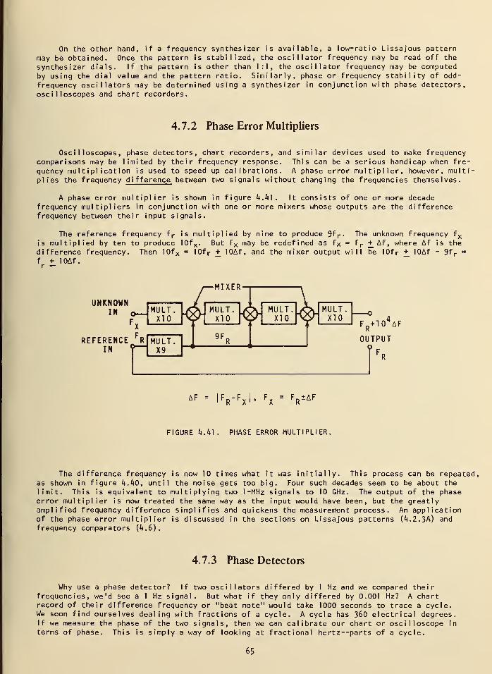
On the other hand, if a frequency synthesizer is available, a low-ratio Lissajous pattern
may be obtained. Once the pattern is stabilized, the oscillator frequency may be read off the
synthesizer dials. If the pattern is other than 1:1, the oscillator frequency may be computed
by using the dial value and the pattern ratio. Similarly, phase or frequency stability of odd-
frequency oscillators may be determined using a synthesizer in conjunction with phase detectors,
oscilloscopes and chart recorders.
4.7.2 Phase Error Multipliers
Oscilloscopes, phase detectors, chart recorders, and similar devices used to make frequencycomparisons may be limited by their frequency response. This can be a serious handicap when fre-
quency multiplication is used to speed up calibrations. A phase error multiplier, however, multi
plies the frequency difference between two signals without changing the frequencies themselves.
A phase error multiplier is shown in figure k.k\. It consists of one or more decadefrequency multipliers in conjunction with one or more mixers whose outputs are the differencefrequency between their input signals.
The reference frequency f r is multiplied by nine to produce 9fp- The unknown frequency fxis multiplied by ten to produce 10fx . But f x may be redefined as fx = f r
+ Af , where Af is the
difference frequency. Then 10f x = 1 Of r + lOAf, and the mixer output will be 10f r + lOAf - 9f r=
f + lOAf.
UNKNOWNIN o—
F„
/— ri i a l n
VMULT.XIO 4 MULT.
XIO iIMULT.XIO & MULT.
XIOFR+10 4
AFX
REFERENCEFR MULT.
X9_ ' OUTPUT
IN cFRR
A F " l
FR-
FX
9 FX
= F +R"
AF
FIGURE Ij.lfl. PHASE ERROR MULTIPLIER.
The difference frequency is now 10 times what it was initially. This process can be repeated,
as shown in figure k.kO, until the noise gets too big. Four such decades seem to be about thelimit. This is equivalent to multiplying two 1 -MHz signals to 10 GHz. The output of the phaseerror multiplier is now treated the same way as the input would have been, but the greatlyamplified frequency difference simplifies and quickens the measurement process. An applicationof the phase error multiplier is discussed in the sections on Lissajous patterns (4.2.3A) andfrequency comparators (4.6).
4.7.3 Phase Detectors
Why use a phase detector? If two oscillators differed by 1 Hz and we compared theirfrequencies, we'd see a 1 Hz signal. But what if they only differed by 0.001 Hz? A chartrecord of their difference frequency or "beat note" would take 1000 seconds to trace a cycle.We soon find ourselves dealing with fractions of a cycle. A cycle has 360 electrical degrees.If we measure the phase of the two signals, then we can calibrate our chart or oscilloscope in
terms of phase. This is simply a way of looking at fractional hertz—parts of a cycle.
65
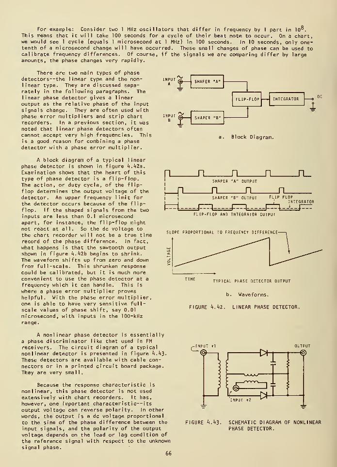
For example: Consider two 1 MHz oscillators that differ in frequency by 1 part in 10°.
This means that it will take 100 seconds for a cycle of their beat note to occur. On a chart,we would see 1 cycle (equals 1 microsecond at 1 MHz) in 100 seconds. In 10 seconds, only one-tenth of a microsecond change will have occurred. These small changes of phase can be used tocalibrate frequency differences. Of course, if the signals we are comparing differ by largeamounts, the phase changes very rapidly.
There are two main types of phasedetectors--the 1 inear type and the non- input
linear type. They are discussed sepa- *
rately in the following paragraphs. Thelinear phase detector gives a linear
output as the relative phase of the inputsignals change. They are often used withphase error multipliers and strip chart input
recorders. In a previous section, it wasnoted that linear phase detectors oftencannot accept very high frequencies. Thisis a good reason for combining a phasedetector with a phase error multiplier.
s- SHAPER "A"
FLIP-FLOP INTEGRATOR
'V.
SHAPER "B"1
a. Block Diagram.
1
A block diagram of a typical linearphase detector is shown in figure 4.42a.
Examination shows that the heart of this
type of phase detector is a flip-flop.The action, or duty cycle, of the flip-
flop determines the output voltage of the
detector. An upper frequency limit for
the detector occurs because of the flip-flop. If the shaped signals from the two
inputs are less than 0.1 microsecondapart, for instance, the flip-flop mightnot react at all. So the dc voltage to
the chart recorder will not be a true time
record of the phase difference. In fact,
what happens is that the sawtooth outputshown in figure 4. 42b begins to shrink.The waveform shifts up from zero and downfrom full-scale. This shrunken responsecould be calibrated, but it is much moreconvenient to use the phase detector at a
frequency which it can handle. This is
where a phase error multiplier proves
helpful. With the phase error multiplier,one is able to have very sensitive full-scale values of phase shift, say 0.01
microsecond, with inputs in the 100-kHzrange.
n JT Jl JT Jl_SHAPER "A" OUTPUT^ JT Jl Jl
i i
SHAPER "B" OUTPUT FLIP FLOP
i INTEGRATOR
FLIP-FLOP ANO INTEGRATOR OUTPUT
SLOPE PROPORTIONAL TO FREQUENCY DIFFERENCE
TIME TYPICAL PHASE DETECTOR OUTPUT
b. Waveforms.
FIGURE 4.42. LINEAR PHASE DETECTOR.
A nonlinear phase detector is essentiallya phase discriminator like that used in FM
receivers. The circuit diagram of a typicalnonlinear detector is presented in figure 4.43-
These detectors are available with cable con-
nectors or in a printed circuit board package.
They are very small.
Because the response characteristic is
nonlinear, this phase detector is not used
extensively with chart recorders. It has,
however, one important character istic--its
output voltage can reverse polarity. In otherwords, the output is a dc voltage proportional
to the sine of the phase difference between the
input signals, and the polarity of the outputvoltage depends on the lead or lag condition of
the reference signal with respect to the unknown
signal phase.66
,-INPUT #1
FIGURE 4.43. SCHEMATIC DIAGRAM OF NONLINEARPHASE DETECTOR.
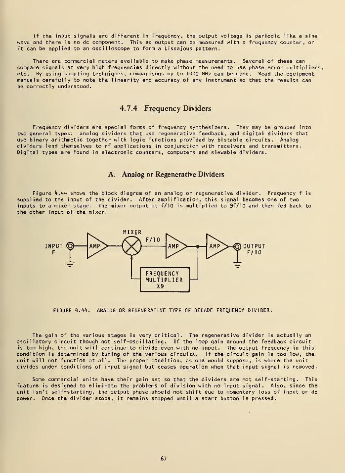
If the input signals are different in frequency, the output voltage is periodic like a sinewave and there is no dc component. This ac output can be measured with a frequency counter, or
it can be applied to an oscilloscope to form a Lissajous pattern.
There are commercial meters available to make phase measurements. Several of these cancompare signals at very high frequencies directly without the need to use phase error multipliers,etc. By using sampling techniques, comparisons up to 1000 MHz can be made. Read the equipmentmanuals carefully to note the linearity and accuracy of any instrument so that the results canbe correctly understood.
4.7.4 Frequency Dividers
Frequency dividers are special forms of frequency synthesizers. They may be grouped into
two general types: analog dividers that use regenerative feedback, and digital dividers thatuse binary arithmetic together with logic functions provided by bistable circuits. Analogdividers lend themselves to rf applications in conjunction with receivers and transmitters.Digital types are found in electronic counters, computers and slewable dividers.
A. Analog or Regenerative Dividers
Figure bAk shows the block diagram of an analog or regenerative divider. Frequency f is
supplied to the input of the divider. After amplification, this signal becomes one of twoinputs to a mixer stage. The mixer output at f/10 is multiplied to 9f/10 and then fed back to
the other input of the mixer.
MIXER
>{
F/10JMDN.
1
1
FREQUENCYMULTIPLIER
X9
AMP OUTPUTF/10
FIGURE k. kk. ANALOG OR REGENERATIVE TYPE OF DECADE FREQUENCY DIVIDER.
The gain of the various stages is very critical. The regenerative divider is actually an
oscillatory circuit though not self-oscillating. If the loop gain around the feedback circuitis too high, the unit will continue to divide even with no input. The output frequency in thiscondition is determined by tuning of the various circuits. If the circuit gain is too low, the
unit will not function at all. The proper condition, as one would suppose, is where the unitdivides under conditions of input signal but ceases operation when that input signal is removed.
Some commercial units have their gain set so that the dividers are not self-starting. Thisfeature is designed to eliminate the problems of division with no input signal. Also, since the
unit isn't self-starting, the output phase should not shift due to momentary loss of input or dc
power. Once the divider stops, it remains stopped until a start button is pressed.
67
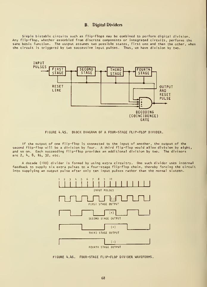
B. Digital Dividers
Simple bistable circuits such as flip-flops may be combined to perform digital division.Any flip-flop, whether assembled from discrete components or integrated circuits, performs thesame basic function. The output assumes two possible states, first one and then the other, whenthe circuit is triggered by two successive input pulses. Thus, we have division by two.
INPUTPULSES
FIRSTSTAGE
•—
*
RESETLINE
SECONDSTAGE
THIRDSTAGE
•—- FOURTHSTAGE
^DOUTPUTANDRESETPULSE
DECODING(COINCIDENCE)
GATE
FIGURE k.kS. BLOCK DIAGRAM OF A FOUR-STAGE FLIP-FLOP DIVIDER.
If the output of one flip-flop is connected to the input of another, the output of the
second flip-flop will be a division by four. A third flip-flop would allow division by eight,and so on. Each succeeding flip-flop provides an additional division by two. The divisorsare 2, k, 8, 16, 32, etc.
A decade (^10) divider is formed by using extra circuitry. One such divider uses internal
feedback to supply six extra pulses to a four-stage flip-flop chain, thereby forcing the circuit
into supplying an output pulse after only ten input pulses rather than the normal sixteen.
123^5678910i_L
[NPUT PULSES
nLnJTJXTMTJTJUFIRST STAGE OUTPUT
SECOND STAGE OUTPUT
( + )
THIRD STAGE OUTPUT
(-)
FOURTH STAGE OUTPUT
FIGURE k.kd. FOUR-STAGE FLIP-FLOP DIVIDER WAVEFORMS,
68
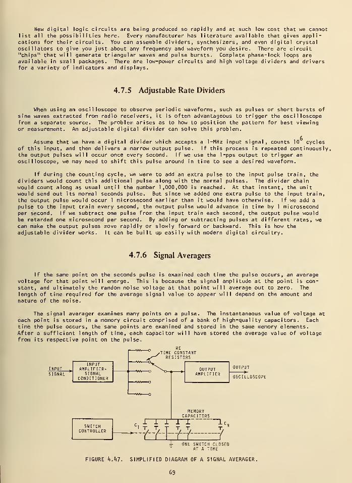
New digital logic circuits are being produced so rapidly and at such low cost that we cannotlist all the possibilities here. Every manufacturer has literature available that gives appli-cations for their circuits. You can assemble dividers, synthesizers, and even digital crystaloscillators to give you just about any frequency and waveform you desire. There are circuit"chips" that will generate triangular waves and pulse bursts. Complete phase-lock loops areavailable in small packages. There are low-power circuits and high voltage dividers and driversfor a variety of indicators and displays.
4.7.5 Adjustable Rate Dividers
When using an oscilloscope to observe periodic waveforms, such as pulses or short bursts of
sine waves extracted from radio receivers, it is often advantageous to trigger the oscilloscopefrom a separate source. The problem arises as to how to position the pattern for best viewingor measurement. An adjustable digital divider can solve this problem.
Assume that we have a digital divider which accepts a 1-MHz input signal, counts 10 cyclesof this input, and then delivers a narrow output pulse. If this process is repeated continuously,the output pulses will occur once every second. If we use the 1 -pps output to trigger an
oscilloscope, we may need to shift this pulse around in time to see a desired waveform.
If during the counting cycle, we were to add an extra pulse to the input pulse train, the
dividers would count this additional pulse along with the normal pulses. The divider chainwould count along as usual until the number 1,000,000 is reached. At that instant, the unitwould send out its normal seconds pulse. But since we added one extra pulse to the input train,the output pulse would occur 1 microsecond earlier than it would have otherwise. If we add a
pulse to the input train every second, the output pulse would advance in time by 1 microsecondper second. If we subtract one pulse from the input train each second, the output pulse wouldbe retarded one microsecond per second. By adding or subtracting pulses at different rates, wecan make the output pulses move rapidly or slowly forward or backward. This is how theadjustable divider works. It can be built up easily with modern digital circuitry.
4.7.6 Signal Averagers
If the same point on the seconds pulse is examined each time the pulse occurs, an averagevoltage for that point will emerge. This is because the signal amplitude at the point is con-stant, and ultimately the random noise voltage at that point will average out to zero. The
length of time required for the average signal value to appear will depend on the amount and
nature of the noise.
The signal averager examines many points on a pulse. The instantaneous value of voltage at
each point is stored in a memory circuit comprised of a bank of high-quality capacitors. Eachtime the pulse occurs, the same points are examined and stored in the same memory elements.After a sufficient length of time, each capacitor will have stored the average value of voltagefrom its respective point on the pulse.
R C
TIME CONSTANTRESISTORS
INPUTSIGNAL
INPUTAMPLIFIER-
SIGNALCONDITIONER
SWITCHCONTROLLER
. Ill1 T. T
OUTPUTAMPLIFIER
OUTPUT>
OSCILLOSCOPE
MEMORYCAPACITORSTT
Tt±kH=l± ONE SWITCH CLOSED
AT A TIME
FIGURE h.kl. SIMPLIFIED DIAGRAM OF A SIGNAL AVERAGER.
69
Each of the memory capacitors is in series with an electronic switch. The switches areclosed and opened by a control circuit, which operates each switch in succession so that onlyone is closed at any given time. Resistors between the input and output amplifiers allow thetime constant of the memory elements to be optimized with respect to the length of the pulse.
As each switch is closed, its associated capacitor charges to the instantaneous voltagepresent at the point on the waveform being examined. That voltage is simultaneously displayedon an oscilloscope. The waveform of the displayed pulse is composed then of many discretevoltage levels read from many storage capacitors.
As one can imagine, the entire process must be carefully synchronized. The switch con-troller is triggered simultaneously with the oscilloscope trigger, and the switching rate is
adjusted nominally to allow a display of all capacitor voltages during one sweep of theoscilloscope beam.
The signal averaging technique allows one to see weak signals in noise without loss ofsignal bandwidth. Commercial instruments are available using the analog method describedabove and also digital techniques. After the signal has been recovered from the noise,measurements can be made to determine the time of arrival, etc. A local clock "tick" can beused to trigger the start of the averaging process.
4.8 PHASE LOCK TECHNIQUES
There are many books and articles on this subject. As mentioned, even integrated circuitsare available to phase lock signals. Here, we only want to acquaint the reader with the conceptof the phase-locked loop and what it will do for our time and frequency measurement problems.If further information is desired, the reader should seek out texts and application notes on thesubject.
The phase-locked loop is made by connecting a phase comparator, integrator, and voltage-controlled oscillator (VCO) . Any one of these blocks can be implemented in many ways.
Functionally, a crystal oscillator that reacts to an input voltage by changing its frequencyis the same as a dc motor that speeds up or slows down as its input voltage is changed.
The net effect of a phase-lock loop can be one of several things. It can change the input
frequency. For example, if the input is 1 MHz, we could put a 100 kHz oscillator in for a VCOand a multiplier in the circuit and have a divider. Or, we could use a 10 MHz VCO and a
divider in the circuit and have a multiplier. We could also change the power level. That is,
a very small input signal could be made to control a powerful output stage. This would give
us a power amplifier.
Typical applications for a phase-locked loop involve the idea of filtering the input
signal. Usually a low-pass filter does this for us. The VCO is connected after the filter.
This prevents high frequency signals (where the noise usually is) from affecting the VCO. So,
if the input is a 1 MHz signal with noise, we can remove the noise and keep the 1 MHz signal.
It's not really that easy or simple, but just an example of what is happening.
Since very narrow bandwidths can be achieved, we could separate one signal from anothereven though they are very close together. If you read articles written in the field of time
and frequency technology, mention is often made of using phase-locked loops to remove noisefrom signals after they have arrived over telephone lines, etc.
An important application of phase-lock techniques is in the VLF tracking receiver. The
application of the loop is to measure the phase of a local oscillator with respect to a received
signal at VLF frequencies. Here the phase-locked loop filters provide an analog phase outputand even synthesizes the necessary frequencies so the receiver can be tuned throughout the VLF
band
.
The block diagram of a simple phase-tracking receiver is shown in figure 4.48. Basically,this receiver adjusts the phase of a local frequency standard to agree with that of a receivedradio signal. The phase adjustment is performed by a phase shifter, which also accepts the
70
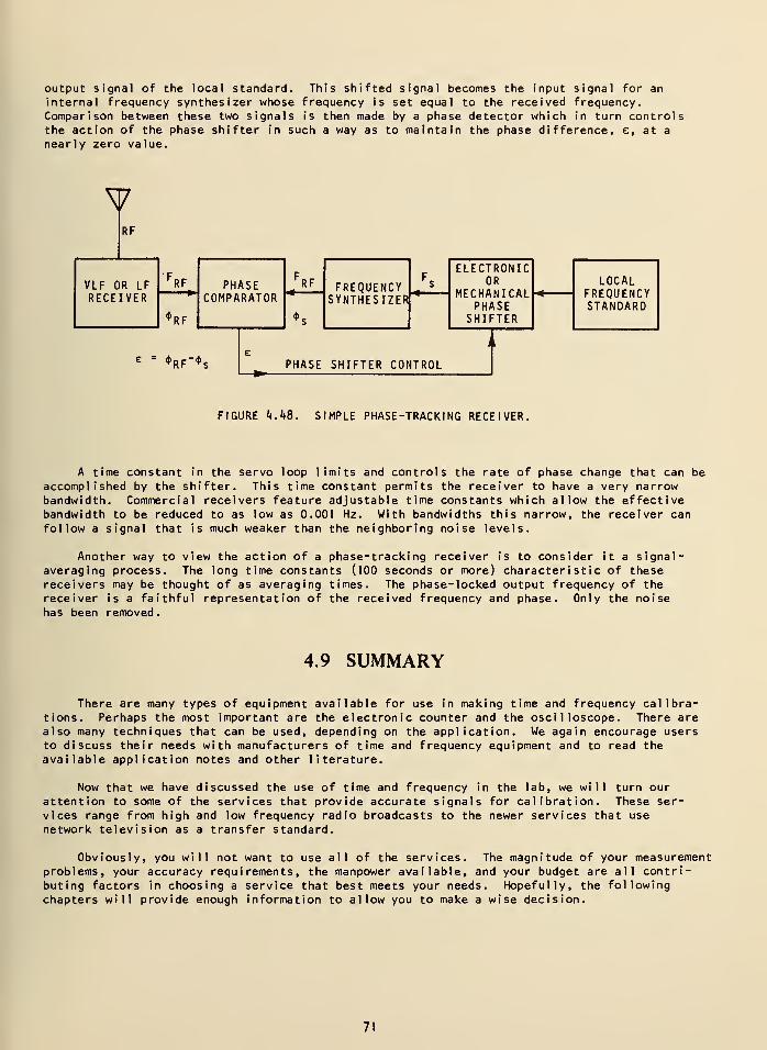
output signal of the local standard. This shifted signal becomes the input signal for an
internal frequency synthesizer whose frequency is set equal to the received frequency.Comparison between these two signals is then made by a phase detector which in turn controlsthe action of the phase shifter in such a way as to maintain the phase difference, e, at a
nearly zero value.
\7RF
VLF OR LFRECEIVER
FRF PHASE
COMPARATOR
FRF FREQUENCY
SYNTHESIZER
Fs
ELECTRONICOR
MECHANICALPHASE
SHIFTER
LOCALFREQUENCYSTANDARD
*RF *s
E =*RF"<>s
e
< ijo— PHASE SHIFTER CONTROL
u
FIGURE It. k8. SIMPLE PHASE-TRACKING RECEIVER.
A time constant in the servo loop limits and controls the rate of phase change that can be
accomplished by the shifter. This time constant permits the receiver to have a very narrowbandwidth. Commercial receivers feature adjustable time constants which allow the effectivebandwidth to be reduced to as low as 0.001 Hz. With bandwidths this narrow, the receiver canfollow a signal that is much weaker than the neighboring noise levels.
Another way to view the action of a phase-tracking receiver is to consider it a signal-averaging process. The long time constants (100 seconds or more) characteristic of thesereceivers may be thought of as averaging times. The phase-locked output frequency of thereceiver is a faithful representation of the received frequency and phase. Only the noisehas been removed.
4.9 SUMMARY
There are many types of equipment available for use in making time and frequency calibra-tions. Perhaps the most important are the electronic counter and the oscilloscope. There arealso many techniques that can be used, depending on the application. We again encourage usersto discuss their needs with manufacturers of time and frequency equipment and to read theavailable application notes and other literature.
Now that we have discussed the use of time and frequency in the lab, we will turn ourattention to some of the services that provide accurate signals for calibration. These ser-vices range from high and low frequency radio broadcasts to the newer services that use
network television as a transfer standard.
Obviously, you will not want to use all of the services. The magnitude of your measurementproblems, your accuracy requirements, the manpower available, and your budget are all contri-buting factors in choosing a service that best meets your needs. Hopefully, the followingchapters will provide enough information to allow you to make a wise decision.
71
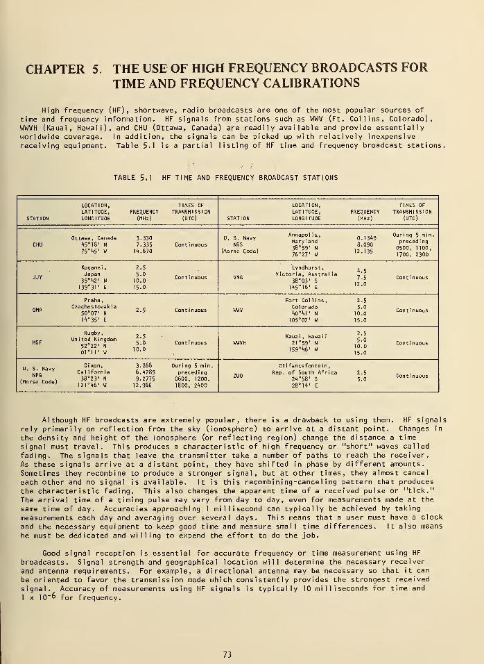
CHAPTER 5 THE USE OF HIGH FREQUENCY BROADCASTS FORTIME AND FREQUENCY CALIBRATIONS
High frequency (HF) , shortwave, radio broadcasts are one of the most popular sources of
time and frequency information. HF signals from stations such as WWV (Ft. Collins, Colorado),WWVH (Kauai, Hawaii), and CHU (Ottawa, Canada) are readily available and provide essentiallyworldwide coverage. In addition, the signals can be picked up with relatively inexpensivereceiving equipment. Table 5.1 is a partial listing of HF time and frequency broadcast stations,
TABLE 5.1 HF TIME AND FREQUENCY BROADCAST STATIONS
LOCATION, TIMES OF
LATITUDE, FREQUENCY TRANSMISSIONSTATION LONGITUDE (MHz) (UTC)
LOCATION, TIMES OF
LATITUDE, FREQUENCY TRANSMISSIONSTATION LONGITUDE (MHz) (UTC)
Ottawa, Canada 3.330CHU It5°l8' N 7.335 Continuous
75oi*5
' W 14.670
., e . Annapolis, . ,-,in During 5 min.U. S. Navy u
K,
' . 1 3^9 .NSS
Maryland „ preceding
,u r , v 38°59' N ,,-,^ 0500, 1100,(Morse Code) ^.^ y
12.135 ]m> 2300
Koganei , 2.5
,„ Japan 5.0 n „.JJY ^ kv N ]0Q Continuous
139°31' E 15.0
Lyndhurst, , _
,,,,- Victoria, Australia ,", . •.
VNG ,»,.,, c 7.5 Continuous3 ° 3 S
12145°16' E
u -°
Praha,
„„. Czechoslovakia _ . . „.OMA „,.,, .. 2.5 Continuous50 U / N
1 ^°35'
E
Fort Col 1 ins, 2.5
,„.,, Colorado 5.0 .WWV OT,. N ,0.0
Continuous
105°02' W 15.0
Rugby,2„„ United Kingdom _* .
MSF ..o,,, ^ 5-0 Continuous- 10orn ' w
lu-u
2.5Kauai , Hawa i
i
WWVH 21°59' N , ^- " Continuous
159-w w |°;°
., , ., Dixon, 3.268 During 5 min.U. S. Navy .,.,'. J
, . , 0r3 '
NprCalifornia 6. "4285 preceding
(w,rL r^=1 38°23' N 9.2775 0600, 1200,(Morse Code)
i 2 l°J+6' W 12.966 1800, 2400
01 ifantsfontein
,
,... Rep. of South Africa 2.5 ,.
ZU0 2i)058 , s 5
-
QContinuous
28° 1 A 1
E
Although HF broadcasts are extremely popular, there is a drawback to using them. HF signals
rely primarily on reflection from the sky (ionosphere) to arrive at a distant point. Changes in
the density and height of the ionosphere (or reflecting region) change the distance a time
signal must travel. This produces a characteristic of high frequency or "short" waves called
fading. The signals that leave the transmitter take a number of paths to reach the receiver.
As these signals arrive at a distant point, they have shifted in phase by different amounts.
Sometimes they recombine to produce a stronger signal, but at other times, they almost cancel
each other and no signal is available. It is this recombining-cancel ing pattern that produces
the characteristic fading. This also changes the apparent time of a received pulse or "tick."
The arrival time of a timing pulse may vary from day to day, even for measurements made at the
same time of day. Accuracies approaching 1 millisecond can typically be achieved by taking
measurements each day and averaging over several days. This means that a user must have a clock
and the necessary equipment to keep good time and measure small time differences. It also means
he must be dedicated and willing to expend the effort to do the job.
Good signal reception is essential for accurate frequency or time measurement using HF
broadcasts. Signal strength and geographical location will determine the necessary receiver
and antenna requirements. For example, a directional antenna may be necessary so that it can
be oriented to favor the transmission mode which consistently provides the strongest received
signal. Accuracy of measurements using HF signals is typically 10 milliseconds for time and
1 x 10"° for frequency.
73
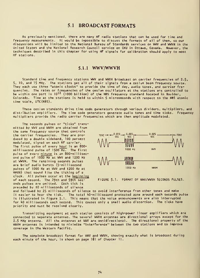
5.1 BROADCAST FORMATS
As previously mentioned, there are many HF radio stations that can be used for time andfrequency measurements. It would be impossible to discuss the formats of all of them, so ourdiscussions will be limited to the National Bureau of Standards services on WWV and WWVH in theUnited States and the National Research Council service on CHU in Ottawa, Canada. However, thetechniques described in this chapter for using HF signals for calibration should apply to mostHF stations.
5.1.1 WWV/WWVH
Standard time and frequency stations WWV and WWVH broadcast on carrier frequencies of 2.5,5, 10, and 15 MHz. The stations get all of their signals from a cesium beam frequency source.They each use three "atomic clocks" to provide the time of day, audio tones, and carrier fre-quencies. The rates or frequencies of the cesium oscillators at the stations are controlled tobe within one part in lO'* (1000 billion) of the NBS frequency standard located in Boulder,Colorado. Time at the stations is held to within 5 microseconds with respect to the NBS atomictime scale, UTC(NBS).
These cesium standards drive time code generators through various dividers, multipliers, anddistribution amplifiers. The time code generators generate audio tones and time ticks. Frequencymultipliers provide the radio carrier frequencies which are then amplitude modulated.
The seconds pulses or "ticks" trans-mitted by WWV and WWVH are obtained from
the same frequency source that controls-TONEthe carrier frequencies. They are pro- tone—'^ -^°— I
°'°° 5|- °-^ 5
duced by a double sideband, 100 percentmodulated, signal on each RF carrier.The first pulse of every hour is an 800-
millisecond pulse of 1500 Hz. The first looo Hz wwv
pulse of every minute is an 800-mi 1 1 isec-
ond pulse of 1000 Hz at WWV and 1200 Hz
at WWVH. The remaining seconds pulsesare brief audio bursts (5~mi 1 1 i secondpulses of 1000 Hz at WWV and 1200 Hz at ,20 ° Hz WVH
WWVH) that sound like the ticking of a
clock. All pulses occur at the beginningof each second. The 29th and 59th sec- FIGURE 5-1. FORMAT OF WWV/WWVH SECONDS PULSES.
onds pulses are omitted. Each tick is
preceded by 10 milliseconds of silenceand followed by 25 milliseconds of silence to avoid interference from other tones and make
it easier to hear the tick. The total ^0-mi 1 1 i second protected zone around each seconds pulse
is illustrated in figure 5.1. This means that the voice announcements are also interrupted
for **0 milliseconds each second. This causes only a small audio distortion. The ticks have
priority and must be received clearly.
Transmitting equipment at each station consists of high-power linear amplifiers which are
connected to separate antennas. The several WWVH antennas are directional arrays except for the
2.5 MHz antenna. All the antennas at WWV are omnidirectional. The directional property of the
WWVH antennas is intended to minimize "interference" between the two stations and to improve
coverage in the Western Pacific.
The complete broadcast format for WWV and WWVH, showing exactly what is broadcast during
each minute of the hour, is shown on page 181 of Chapter 11.
Ik

5.1.2 CHU
Canada has many frequency and time services that are quite similar to those of the U. S.
The Canadian HF broadcast station near Ottawa has the call letters CHU. Its signals can beheard over much of the U. S. and are a valuable alternative to the WWV signals. It has the samepropagation characteristics and the same receiving techniques are used. Wherever applicable,mention is made of the Canadian signals in this book.
The CHU signals differ from those of the U. S. stations in two ways. They are not in thestandard frequency bands (see below) and they use a different format. The format is principallyvoice and ticks. At CHU, dual cesium frequency sources are used to generate the carriers andthe seconds pulses. Two systems are used to complement each other in cases of maintenance orfailure. The output from the cesium osci 1 lator' is fed to a solid state frequency synthesizerwhich produces the 3330, 7335, and H670 kHz carrier signals for the transmitters.
The three excitation frequencies are fed into a transmitter room and terminated in a panelwhere each frequency is coupled into two transmitters (main and standby) operating on thatfrequency. A 100 kHz signal is fed into one of two digital clocks where it is divided intoseconds pulses of 1000 Hz tone. The clock gates out the 51st to 59th second pulses of eachminute to permit the voice announcements to be inserted, and also gates out the 29th pulse to
identify the half-minute point.
The same 100 kHz signal is fed into a "talking clock," where it is divided down to 50 Hz
and amplified to a power level that will operate a synchronous motor. The motor drives a
magnetic drum on which the voice announcements are recorded. Two talking clocks are used. One
announces the station identification and time in English, and repeats the time in French. The
other announces the station identification and time in French, and repeats the time in English.
The format is shown in figure 5.2.
CHU DATA TRANSMISSION SEQUENCE
26 27 28 29 30 31 60 1 2 3 4 5 6 7 a 9 10 11 12 13
tttttt-4tKVOICE RECORDINGHOURS MINS.'>Itt-4tK VOICE RECORDING
'HOURS — EXACTLY'>tt 1st to 10th PULSES (INCL.)1 OMITTED
TTT
NOTE: VOICE RECORDINGS ALTERNATE IN FRENCH AND ENGLISH:
"CHU CANADA, EASTERN STANDARD TIME HOURS MINUTES
"CHU CANADA, HEURE NORMALE DE L'EST HEURES MINUTES
"CHU CANADA, EASTERN STANDARD TIME HOURS EXACTLY"
HEURES MINUTES" (EVEN MINUTES)
HOURS MINUTES" (ODO MINUTES)
HEURES PRECISES" (ON THE HOURI
FIGURE 5.2. CHU BROADCAST FORMAT.
In 1975, CHU converted its operation to single sideband. It now broadcasts upper sideband
with full carrier. This is called the 3A3H mode. Users can still get the carrier as a frequency
standard and an ordinary AM radio will allow reception of the audio signals.
A time code is now being tested on CHU. It appears in the 31st to the 39th seconds pulses
of each minute. The modulation is the commercial 300 baud FSK (frequency shift keying) at fre-
quencies of 2025 and 2225 Hz. The code is a modified ASCII in which each 11-bit character con-
tains two BCD digits, with one start bit and two stop bits. The first digit is the number 6 for
identification, which should be verified in the receiving clock, and the remaining 9 digits give
the day, hour, minute and second of UTC . The entire message is then repeated in order that the
receiving clock can check for identical messages before updating. The code ends, and update
occurs at 0.500s. This 0.500s must be added in, along with the time zone hour, to give the
correct time. The same code is also available by telephone. Details can be obtained by writing
to the National Research Council, Ottawa, Ontario, Canada.
75
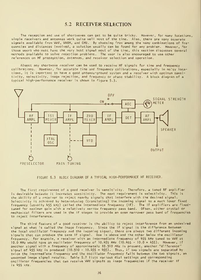
5.2 RECEIVER SELECTION
The reception and use of shortwaves can get to be quite tricky. However, for many locations,simple receivers and antennas work quite well most of the time. Also, there are many separatesignals available from WWV, WWVH, and CHU. By choosing from among the many combinations of fre-quencies and distances involved, a solution usually can be found for any problem. However, forthose users who must have the very best signal most of the time, this section discusses severalmethods available to solve reception problems. The user is also encouraged to use otherreferences on HF propagation, antennas, and receiver selection and operation.
Almost any shortwave receiver can be used to receive HF signals for time and frequencycalibrations. However, for accurate time and frequency calibrations, especially in noisy loca-tions, it is important to have a good antenna-ground system and a receiver with optimum sensi-tivity, selectivity, image rejection, and frequency or phase stability. A block diagram of a
typical high-performance receiver is shown in figure 5-3.
VRF
AMPL
6
1STMIXER
XTALOSC
OFF
ON-o-*-o-
IF
AMPL2ND
MIXERIF
AMPL
AGC
SIGNAL1U//A METER
DET
STRENGTH
VFO
SPEAKER
6
OUTPUT
bPRESELECTOR MAIN TUNING
FIGURE 5.3 BLOCK DIAGRAM OF A TYPICAL HIGH-PERFORMANCE HF RECEIVER.
The first requirement of a good receiver is sensitivity. Therefore, a tuned RF amplifier
is desirable because it increases sensitivity. The next requirement is selectivity. This is
the ability of a receiver to reject nearby signals that interfere with the desired signal.
Selectivity is achieved by heterodyning (translating) the incoming signal to a much lower fixed
frequency (usually 455 kHz) called the intermediate frequency (IF). The IF amplifiers are fixed-
tuned for maximum gain with a relatively narrow frequency pass band. Often, either crystal or
mechanical filters are used in the IF stages to provide an even narrower pass band of frequencies
to reject interference.
The third feature of a good receiv
signal at what is called the image freq
the local oscillator frequency and the
signals that can produce the same IF si
frequency. For example, a receiver wit10.0 MHz would have an oscillator frequ
another signal with a frequency of appr
signal of 455 kHz is produced (10.910 -
twice the intermediate frequency and th
unwanted image signal results. Table 5
oscillator frequencies that can receive
is 455 kHz.
er is the ability to reject interference from an undesired
uency. Since the IF signal is the difference betweenincoming signal, there are always two different incominggnal. One is above and the other below the oscillatorh an intermediate frequency of 455 kHz tuned to WWV at
ency of 10.455 MHz (10.455 - 10.0 = 455). However, if
oximately 10.910 MHz is present, another "difference"
10.455 = 455). Thus, if two signals are separated by
e oscillator frequency falls between the two signals, an
2 lists various dial settings and correspondingWWV signals as image frequencies if the receiver IF
76
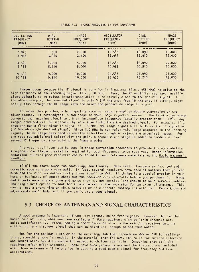
TABLE 5.2 IMAGE FREQUENCIES FOR WWV/WWVH
OSCILLATORFREQUENCY
(MHz)
DIALSETTING(MHz)
IMAGE
FREQUENCY(MHz)
OSCILLATORFREQUENCY
(MHz)
DIALSETTING(MHz)
IMAGE
FREQUENCY(MHz)
2.045
2.955
1.5903.410
2.5002.500
14.545
15.455
14.090
15.910
15.00015.000
4.5455.455
4.0905.910
5.0005.000
19.54520.455
19.09020.910
20.00020.000
9.54510.455
9.09010.910
10.00010.000
24.54525.455
24.09025.910
25.00025.000
Images occur because the IF signal is very low in frequency (i.e., 455 kHz) relative to thehigh frequency of the incoming signal (i.e., 10 MHz). Thus, the RF amplifier may have insuffi-cient selectivity to reject interference which is relatively close to the desired signal. In
the above example, the unwanted signal is only 0.910 MHz away from 10 MHz and, if strong, mighteasily pass through the RF stage into the mixer and produce an image IF signal.
To solve this problem, a high quality receiver usually employs double conversion or twomixer stages. It heterodynes in two steps to make image rejection easier. The first mixer stageconverts the incoming signal to a high intermediate frequency (usually greater than 1 MHz). Anyimages produced will be separated by more than 2 MHz from the desired signal. For example, if areceiver has a first mixer IF signal of 1.5 MHz, the image signal will be twice the IF signal or3.0 MHz above the desired signal. Since 3.0 MHz is now relatively large compared to the incomingsignal, the RF stage pass band is usually selective enough to reject the undes i red images. Forthe required additional selectivity and gain, a second mixer stage is added to produce a lowersecond IF frequency, thus solving the image problem.
A crystal oscillator can be used in these conversion processes to provide tuning stability.A separate oscillator crystal is required for each frequency to be received. Other informationregarding wel 1 -des igned receivers can be found in such reference materials as the Radio Amateur 's
Handbook .
If all the above seems too confusing, don't worry. Many small, inexpensive imported anddomestic receivers work very well. In fact, several receivers have special buttons that you canpush and the receiver automatically tunes itself to WWV. If timing is a special problem in yourhome or business, of course check out the receiver very carefully before you purchase it. Imageand interference signals come and go so they may not persist long enough to be a serious problem.The single best option to look for in a receiver is the provision for an external antenna. Thismay be just a short wire on the windowsill or an elaborate rooftop installation. Fancy knobs andadjustments won't help much if you can't get a good signal.
5.3 CHOICE OF ANTENNAS AND SIGNAL CHARACTERISTICS
A good antenna is important if you want strong, noise-free signals. However, follow thebasic rule of "using what you have available." Many receivers with built-in antennas workquite satisfactorily. Often, adding a short piece of wire to the existing receiver antennawill bring in a stronger signal that can be heard well enough to set your watch.
But for the serious listener or the metrology lab that depends on WWV or CHU for calibra-tions, something more is needed. In the material that follows, the rules for antenna selectionand installation are discussed with respect to choices available. Companies that sell WWVreceivers often offer antennas. These have been proven by use and the instructions includedwith those antennas will help a lot in getting a good usable signal for frequency and timecal ibrations .
77
The signal power as received at great distances from HF stations may be relatively weak.As the distance is increased, the signal decreases in strength so an antenna with maximumefficiency produces the best results. Radio waves arrive at different vertical angles, calledthe wave or radiation angle. The wave angle of an arriving signal depends on the distancebetween the transmitting and receiving stations and also on the height of the ionosphere. Thecloser the receiving station and the higher the ionosphere, the larger the wave angle. There-fore, an antenna should be selected and oriented that favors the wave angle (elevation) as wellas the direction (azimuth). Determining wave angles is discussed more fully in Section 5.6.
WWV, WWVH, and CHU transmit on a number of frequencies. Because of changes in ionosphericconditions, which sometimes adversely affect the signal transmissions, most receivers are notable to pick up the signals on all frequencies at all times in all locations. Except duringtimes of severe magnetic disturbances, howevei
—
which make radio transmissions almost impossible--users should be able to receive the signal on at least one of the broadcast frequencies. As a
general rule, frequencies above 10 MHz provide the best daytime reception while the lowerfrequencies are best for nighttime reception.
An all-band antenna capable of covering the entire HF band is commercially available.These are used for around-the-clock communication purposes where the entire HF band must be usedfor maximum reliability. Such an antenna is very large and cumbersome as well as expensive.Depending on location, an antenna and a receiver capable of receiving two or more frequencies maybe required. Any of the different WWV frequencies transmitted may be received depending upondistance, time of day, month, season, and sunspot cycle. Each frequency will be discussed withthe type of antenna most suitable for its reception. Although WWV and WWVH are not currentlybroadcasting on 20 and 25 MHz, these frequencies are also discussed.
In the following discussion, mention is made of sunspot cycles. These cycles occur with a
periodicity of about every eleven years. Propagation characteristics at high frequencies aregreatly affected by the sunspot cycles. One solution to the problem is to select another fre-quency that will work and to ignore the ones that won't. For those users who want to understandthe propagation effects and to counteract the coming sunspot cycles by antenna selection and
placement, we recommend further reading on this subject. Information on sunspots is availablefrom the Space Environment Lab, NOAA , U. S. Department of Commerce. We are currently (1977)experiencing a minimum in the 11-year sunspot cycle. Previous minimums occurred in 195^ and 1965
The corresponding maximums were in 1958 and 1969, and another will probably occur in 1 980
.
ANTENNAS FOR THE 2.5 TO 3-330 MHz RANGE . Signals at these frequencies have a very short
range during the day because of groundwave propagation limitations. Daytime use is limited to
locations within one to two hundred miles from the transmitter. They become useful at night,however, especially during the winter season in the higher latitudes where longer nights prevail.Reception is then possible over distances of several thousand miles.
The vertical quarter-wavelength monopole antenna has a radiation pattern that favors recep-
tion at low wave angles and is very effective in receiving long distance skywave signals normallyarriving at angles of 20 degrees or less. This antenna is not effective for reception of short-range skywave signals with large wave angles, but it is useful for receiving weak groundwavesignal s.
For nighttime reception on paths up to several thousand miles, the skywave is predominantand a horizontal half-wavelength antenna is recommended. The antenna should be located a quarter-wavelength or higher above ground and separated from possible interfering reflecting obstacles.The quarter-wavelength vertical antenna and the half-wavelength horizontal dipole antenna areillustrated in figure 5-^- To get antenna dimensions for the CHU frequencies, refer to antennamanuals such as those published by the American Radio Relay League.
ANTENNAS FOR THE 3-330 TO 5-0 MHz RANGE . These frequencies can be received at greaterdistances than the 2.5 MHz frequency throughout the day or night, especially during minimumsunspot cycle. Reception is possible up to 1000 miles under ideal conditions, but under normal
conditions, daytime propagation conditions limit its useful range. Therefore, reception is
usually limited to less than 1000 miles during the day. During the night, 5 MHz is a very useful
frequency for long-range reception except during maximum sunspot cycle. It is excellent during
early dawn and early evenings in the winter months when the signal path is in darkness. Hori-
zontal dipole antennas are a good choice for this band. Users should also consider the
possibility of a multiband antenna.
78
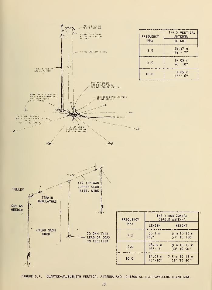
WOODEN I'GLF
GUY AS Nl FDED
TASTLN C ¥ I. BOLT• TO 2x4 YARD ARM
STRAIN INSULATORSAT [NO Or VLRTICALANTENNA
10 AUG COPPER (110)
1 OP MORE PA01ALSEQI'AI L Y SPACTO AR0LT1D
irm pointi 1
6- = 10 AUG COPPER)
URAP F 1NDS OF RAU I ALSAROUND 60d COMMON NAAN!) POUND PLUSHWITH GROUND
URAP AND SOLDCRINNER COND OF COAX
OUER ENO OF VERTICAL
HIRE FROM BRAID SOLDEREDGND RADIALS
FREQUENCYMHz
1/4 A VERTICALANTENNA
HEIGHT
2.528.37 m94'- 7"
5-014.05 m46 ' - 1
0"
10.07.05 m
23'- 6"
RG-S8 COAX
PULLEY
GUY ASNEEDED
/
STRAININSULATORS
MYLAR SASHCORD
,
#14-#12 AWGCOPPER CLADSTEEL WIRE
70 OHM TWINLEAD OR COAXTO RECEIVER
FREQUENCYMHz
1/2 X HORIZONTALDIPOLE ANTENNA
LENGTH HEIGHT
2.556.1 m 15 m TO 30 m187' 50' TO 100'
5-028.07 m 9 m TO 15 m93'- 7" 30' TO 50'
10.014.05 m 7- 5m TO 15m46' -10" 25' TO 50'
FIGURE 5.4. QUARTER-WAVELENGTH VERTICAL ANTENNA AND HORIZONTAL HALF-WAVELENGTH ANTENNA,
79
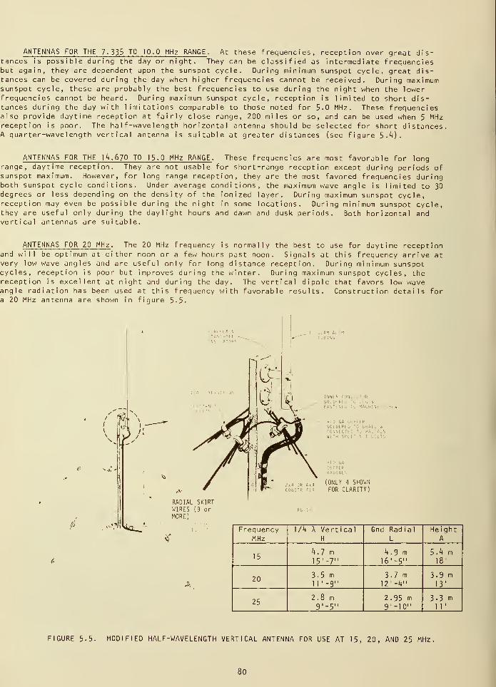
ANTENNAS FOR THE 7-335 TO 10.0 MHz RANGE . At these frequencies, reception over great dis-tances is possible during the day or night. They can be classified as intermediate frequenciesbut again, they are dependent upon the sunspot cycle. During minimum sunspot cycle, great dis-tances can be covered during the day when higher frequencies cannot be received. During maximumsunspot cycle, these are probably the best frequencies to use during the night when the lowerfrequencies cannot be heard. During maximum sunspot cycle, reception is limited to short dis-tances during the day with limitations comparable to those noted for 5.0 MHz. These frequenciesalso provide daytime reception at fairly close range, 200 miles or so, and can be used when 5 MHzreception is poor. The half-wavelength horizontal antenna should be selected for short distances.A quarter-wavelength vertical antenna is suitable at greater distances (see figure 5.4).
ANTENNAS FOR THE 14.670 TO 15.0 MHz RANGE . These frequencies are most favorable for longrange, daytime reception. They are not usable for short-range reception except during periods ofsunspot maximum. However, for long range reception, they are the most favored frequencies duringboth sunspot cycle conditions. Under average conditions, the maximum wave angle is limited to 30degrees or less depending on the density of the ionized layer. During maximum sunspot cycle,reception may even be possible during the night in some locations. During minimum sunspot cycle,they are useful only during the daylight hours and dawn and dusk periods. Both horizontal andvertical antennas are suitable.
ANTENNAS FOR 20 MHz . The 20 MHz frequency is normally the best to use for daytime receptionand will be optimum at either noon or a few hours past noon. Signals at this frequency arrive atvery low wave angles and are useful only for long distance reception. During minimum sunspotcycles, reception is poor but improves during the winter. During maximum sunspot cycles, thereception is excellent at night and during the day. The vertical dipole that favors low waveangle radiation has been used at this frequency with favorable results. Construction details fora 20 MHz antenna are shown in figure 5-5-
I' DIAH Al 11
TUB I riCi
,v
RADIAL SKIRTWIRES (9 or
MORE)
.^Vi£^_
I N N ( K CON I C T Ut<
ioiD' ks o ro i . \
." V '.|| :•.
• 10 GA C0PCE M
SOL UL Ri :
I
' HAL1AL1H1TH SI'l IT-N
= 10 GAC0PPEK
I
a 0R 4 „ 4(ONLY 4 SHOWN
•isth riR FOR CLARITY)
FrequencyMHz
1/4 X VerticalH
Gnd Rad i a 1
L
HeightA
154.7 m15'-7"
4.9 m
l6'-5"5.4 m18'
203-5 m
1
1 ' -9"3-7 m12'-4"
3-9 m13'
252.8 m9.-5.1
2.95 m9" -10"
3-3 m1 1
'
FIGURE 5.5. MODIFIED HALF-WAVELENGTH VERTICAL ANTENNA FOR USE AT 15, 20, AND 25 MHz,
80
ANTENNAS FOR 25 MHz . The 25 MHz frequency is best during daylight hours except during the
summer. Reception is especially good during maximum sunspot cycle and very poor during minimumsunspot cycle. It is used only for long distance reception because a low radiation angle is
required for the signal to be returned back to the earth from the ionosphere. Design details of
a different vertical antenna for use at 25 MHz are also shown in figure 5.5-
VERTICAL ANTENNA CONSTRUCTION . The vertical antenna which is favorable to low wave-anglereception is preferable to the horizontal hal f -wavelength antenna and can readily be constructedas shown in figure 5.5- The dimension of the ground radials and orientation as shown should be
used to yield approximately a 50 ohm antenna impedance. For a 70 - 90 ohm antenna, the half-
wavelength dipole mounted vertically will yield approximately the correct impedance. In order to
prevent interaction between the feed line and the lower half of the dipole, which disturbs the
radiation pattern, extend the feed line horizontally outward several feet from the antenna beforedropping it vertically to the ground.
5.4 USE OF HF BROADCASTS FOR TIME CALIBRATIONS
Now that we have a receiver and an antenna, we can proceed to make time calibrations. If
your accuracy requirements are low, you can use the voice time-of-day announcements. However,if you want higher accuracy, you will have to measure the seconds ticks or decode the WWV/WWVHtime code.
5.4.1 Time-of-Day Announcements
Time of day is available from many sources in the United States and Canada. Radio and
television stations mention the time frequently and, in fact, use the time of day to scheduletheir own operations. The telephone companies offer time-of-day services in most locations.
But where does the time come from?
Most time-of-day services in the U. S. start at the National Bureau of Standards. An NBS
telephone service is available by calling (303) 499-71 1 1 • In addition, WWV and WWVH broadcastvoice time-of-day announcements once each minute. This is also the case for CHU where the timeannouncements are given alternately in French and English. Using the WWV voice announcement andthe tone following the words, "At the tone, XXXX hours XXXX minutes Coordinated Universal Time,"a person can check a wall clock or wristwatch to within a fraction of a second. The UTC timethat .is announced can be converted to local time by using the map in Chapter 2.
5.4.2 Using the Seconds Ticks
For accurate time recovery, we cannot just listen. We must rely on electronic equipment.By using an electronic oscilloscope to see the ticks, the user can set clocks with much greateraccuracy than is possible by only listening to the ticks. An oscilloscope is a necessity whendealing with noisy signals that fade.
The following describes ways to get time of day with resolutions better than 1 millisecond(1000 microseconds) by using an oscilloscope. Under very favorable conditions, it is possibleto establish time synchronization to about 100 microseconds. In each case, path and equipmenttime delay corrections are necessary for accurate results.
In order to achieve the best results in any of these measurement methods, the followingguidelines are recommended:
1. Make your measurements at the same time every day.
2. Avoid twilight hours when the ionosphere is the least stable.
3. Use the highest carrier frequency which provides consistently good reception.
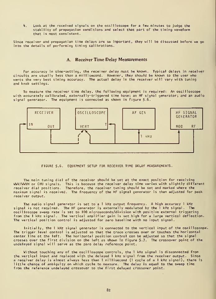
k. Look at the received signals on the oscilloscope for a few minutes to judge the
stability of propagation conditions and select that part of the timing waveformthat is most consistent.
Since receiver and propagation time delays are so important, they will be discussed before we go
into the details of performing timing calibrations.
A. Receiver Time Delay Measurements
For accuracy in time-setting, the receiver delay must be known. Typical delays in receiver
circuits are usually less than a millisecond. However, they should be known to the user whowants the very best timing accuracy. The actual delay in the receiver will vary with tuning
and knob settings.
To measure the receiver time delay, the following equipment is required: An oscilloscope
with accurately calibrated, externally-triggered time base; an HF signal generator; and an audio
signal generator. The equipment is connected as shown in figure 5.6-
»
RECEIVER
INOUT
OSCILLOSCOPE
VERT-+—
AF GEN HF SIGNALGENERATOR
MOD RF
n 1 kHz
i i
FIGURE 5.6. EQUIPMENT SETUP FOR RECEIVER TIME DELAY MEASUREMENTS.
The main tuning dial of the receiver should be set at the exact position for receiving
WWV/WWVH or CHU signals. This is because the receiver delay time varies with slightly different
receiver dial positions. Therefore, the receiver tuning should be set and marked where the
maximum signal is received. The frequency of the HF signal generator is then adjusted for peak
receiver output.
The audio signal generator is set to a 1 kHz output frequency. A high accuracy 1 kHz
signal is not required. The HF generator is externally modulated by the 1 kHz signal. The
oscilloscope sweep rate is set to 100 microseconds/division with positive external triggeringfrom the 1 kHz signal. The vertical amplifier gain is set high for a large vertical deflection.
The vertical position control is adjusted for zero baseline with no input signal.
Initially, the 1 kHz signal generator is connected to the vertical input of the oscilloscope.
The trigger level control is adjusted so that the trace crosses over or touches the horizontal
center line at the left. The horizontal position control can be adjusted so that the signal
crosses over the first division on the left as shown in figure 5.7- The crossover point of the
undelayed signal will serve as the zero delay reference point.
Without touching any of the oscilloscope controls, the 1 kHz signal is disconnected from
the vertical input and replaced with the delayed 1 kHz signal from the receiver output. Since
a receiver delay is almost always less than 1 millisecond (1 cycle of a 1 kHz signal), there is
little chance of ambiguity on which cycle to measure. The delay is equal to the sweep time
from the reference undelayed crossover to the first delayed crossover point.
82
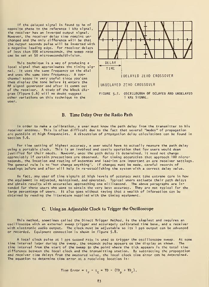
If the delayed signal is found to be of
opposite phase to the reference 1 kHz signal,the receiver has an inverted output signal.However, the receiver delay time remains un-
changed and the only difference will be that
the output seconds pulse will be inverted witha negative leading edge. For receiver delaysof less than 500 microseconds, the sweep rate
can be set at 50 microseconds/division.
This technique is a way of producing a
local signal that approximates the timing sig-
nal. It uses the same frequency on the dial
and uses the same tone frequency. A two-
channel scope is very useful since you' can
then display the tone before it enters the
RF signal generator and after it comes outof the receiver. A study of the block dia-gram (figure 5.6) will no doubt suggestother variations on this technique to the
user.
IM
DELAY
TIME
DELAYED ZERO CROSSOVER
UNDELAYED ZERO CROSSOVER
FIGURE 5.7- OSCILLOGRAM OF DELAYED AND UNDELAYED1 kHz SIGNAL.
B. Time Delay Over the Radio Path
In order to make a calibration, a user must know the path delay from the transmitter to his
receiver antenna. This is often difficult due to the fact that several "modes" of propagationare possible at high frequencies. A discussion of propagation delay calculations can be found in
section 5.6.
For time setting of highest accuracy, a user would have to actually measure the path delayusing a portable clock. This is an involved and costly operation that few users would deemjustified for their needs. However, once the path delay is determined, it need not changeappreciably if certain precautions are observed. For timing accuracies that approach 100 micro-seconds, the location and routing of antennas and lead-ins are important as are receiver settings.The general rule is to "not change anything". If changes must be made, careful records ofreadings before and after will help in re-establishing the system with a correct delay value.
In fact, any user of time signals at high levels of accuracy must take extreme care in howthe equipment is adjusted, maintained, and operated. Typical users estimate their path delaysand obtain results with accuracies approaching one millisecond. The above paragraphs are in-
tended for those users who want to obtain the very best accuracy. They are not typical for the
large percentage of users. It also goes without saying that a wealth of information can be
obtained by reading the literature supplied with the timing equipment.
C. Using an Adjustable Clock to Trigger the Oscilloscope
This method, sometimes called the Direct Trigger Method, is the simplest and requires an
oscilloscope with an external sweep trigger and accurately calibrated time base, and a receiverwith electronic audio output. The clock must be adjustable so its 1 pps output can be advancedor retarded. Equipment connection is shown in figure 5-8.
A local clock pulse at 1 pps second rate is used to trigger the oscilloscope sweep. At sometime interval later during the sweep, the seconds pulse appears on the display as shown. Thetime interval from the start of the sweep to the point where the tick appears is the total timedifference between the local clock and the transmitting station. By subtracting the propagationand receiver time delays from the measured value, the local clock time error can be determined.The equation to determine time error at a receiving location is:
Time Error = t - t = TD - (TD + TD )
,
r t p r
83
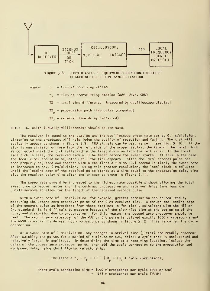
V
HFRECEIVER
SECONDSPULSE w
ORTICK
OSCILLOSCOPE
VERTICAL TRIGGER
1 pps LOCALFREQUENCYSOURCE
OR CLOCK
FIGURE 5.8. BLOCK DIAGRAM OF EQUIPMENT CONNECTION FOR DIRECTTRIGGER METHOD OF TIME SYNCHRONIZATION.
where: t = time at receiving stationr
t = time at transmitting station (WWV, WWVH, CHU)
TD = total time difference (measured by oscilloscope display)
TD = propagation path time delay (computed)
TD = receiver time delay (measured)
NOTE: The units (usually milliseconds) should be the same.
The receiver is tuned to
Listening to the broadcast wi
1
typically appear as shown in f
tick is one division or more f
is corrected until the tick fa
time tick is late, the receivethe local clock should be adjubeen properly adjusted and appis increased to say, 5 ms/diviuntil the leading edge of the
plus the receiver delay time a
the station and the oscilloscope sweep rate set at 0.1 s/division.1 help judge the quality of reception and fading. The tick will
igure 5-9. CHU signals can be used as well (see fig. 5-10). If the
rom the left side of the scope display, the time of the local clocklis within the first division from the left side. If the local
d tick will be heard before the sweep starts. If this is the case,
sted until the tick appears. After the local seconds pulse has
ears within the first division (0.1 second in time), the sweep ratesion. Using this greater resolution, the local clock is adjustedreceived pulse starts at a time equal to the propagation delay time
fter the trigger as shown in figure 5.11.
The sweep rate should be increased to the highest rate possible without allowing the total
sweep time to become faster than the combined propagation and receiver delay time less the
5 milliseconds to allow for the length of the received seconds pulse.
With a sweep rate of 1 ms/division, for example, greater resolution can be realized by
measuring the second zero crossover point of the 5 ms received tick. Although the leading edgeof the seconds pulse as broadcast from these stations is "on time", coincident with the NBS orCHU standard, it is difficult to measure because of the slow rise time at the beginning of theburst and distortion due to propagation. For this reason, the second zero crossover should be
used. The second zero crossover of the WWV or CHU pulse is delayed exactly 1000 microseconds and
the WWVH crossover is delayed 833 microseconds as shown in figure 5.12. This is called the cyclecorrect ion.
At a sweep rate of 1 ms/division, any changes in arrival time (jitter) are readily apparent.After watching the pulses for a period of a minute or two, select a cycle that is undistorted andrelatively larger in amplitude. In determining the time at a receiving location, include thedelay of the chosen zero crossover point, then add the cycle correction to the propagation andequipment delay using the following relationship:
Time Error = t - t = TD - (TD + TD + cycle correction),r t p r '
Where cycle correction time = 1000 microseconds per cycle (WWV or CHU)= 833 microseconds per cycle (WWVH)
8k
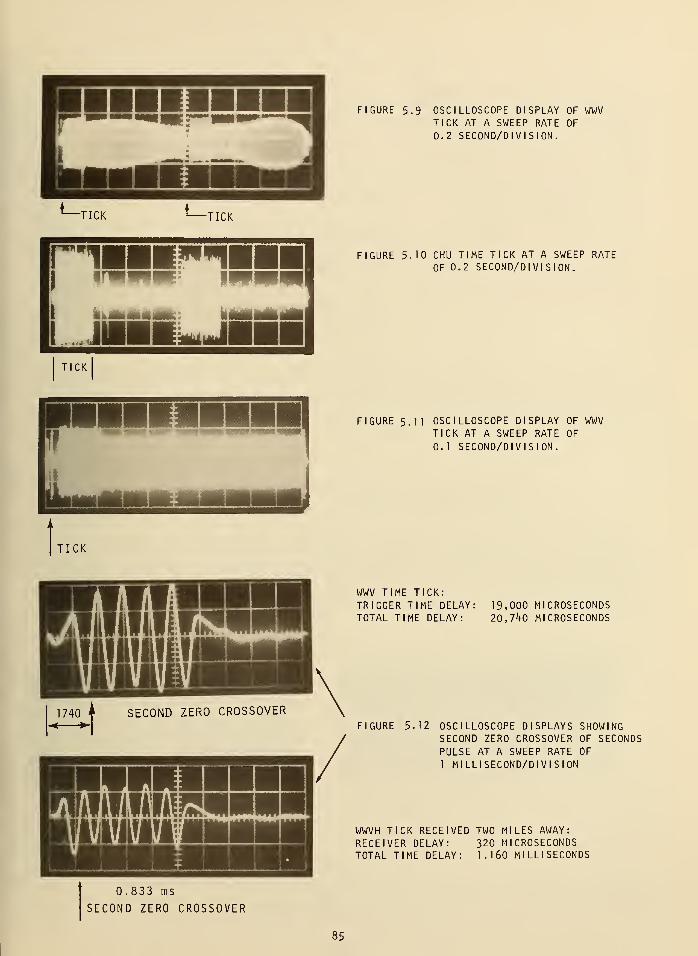
FIGURE 5-9 OSCILLOSCOPE DISPLAY OF WWVTICK AT A SWEEP RATE OF
0.2 SECOND/DIVISION.
"TICK TICK
Inmw^i wt/f
'
J1H1BHHK* 11
TICK
FIGURE 5.10 CHU TIME TICK AT A SWEEP RATE
OF 0.2 SECOND/DIVISION.
FIGURE 5.11 OSCILLOSCOPE DISPLAY OF WWVTICK AT A SWEEP RATE OF
0.1 SECOND/DIVISION.
WWV TIME TICK:
TRIGGER TIME DELAY: 19,000 MICROSECONDSTOTAL TIME DELAY: 20, IkO MICROSECONDS
FIGURE 5.12 OSCILLOSCOPE DISPLAYS SHOWINGSECOND ZERO CROSSOVER OF SECONDSPULSE AT A SWEEP RATE OF
1 MILLISECOND/DIVISION
WWVH TICK RECEIVED TWO MILES AWAY:RECEIVER DELAY: 320 MICROSECONDSTOTAL TIME DELAY: 1.160 MILLISECONDS
0.833 ms
SECOND ZERO CROSSOVER
85
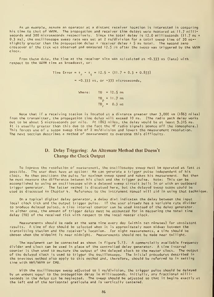
As an example, assume an operator at a distant receiver location is interested in comparinghis time to that of WWVH. The propagation and receiver time delays were measured as 11.7 milli-seconds and 300 microseconds respectively. Since the total delay is 12.0 milliseconds (11.7 ms +
0.3 ms) , the oscilloscope sweep rate was set at 2 ms/division for a total sweep time of 20 ms—slightly greater than the propagation delay + receiver delay + 5 ms total. The second zerocrossover of the tick was observed and measured 12.5 ms after the sweep was triggered by the WWVHclock.
From these data, the time at the receiver site was calculated as -0.333 ms (late) withrespect to the WWVH time as broadcast, or:
Time Error = t - t = 12.5 - (11.7 + 0.3 + 0.833)
= -0.333 ms , or -333 microseconds,
Where: TO = 1 2 . 5 ms
TD = 1 1 .7 msP
TD = 0.3 msr
Note that if a receiving station is located at a distance greater- than 3,000 km (1863 miles)from the transmitter, the propagation time delay will exceed 10 ms . (The radio path delay worksout to be about 5 microseconds per mile. At 1863 miles, the delay would be at least 9-315 ms
.
It is usually greater than this due to the fact the HF radio signals bounce off the ionosphere.)This forces use of a scope sweep time of 2 ms/division and lowers the measurement resolution.The next section describes a method of measurement to overcome this difficulty.
D. Delay Triggering: An Alternate Method that Doesn't
Change the Gock Output
To improve the resolution of measurement, the oscilloscope sweep must be operated as fast as
possible. The user does have an option: He can generate a trigger pulse independent of his
clock. He then positions the pulse for maximum sweep speed and makes his measurement. But then
he must measure the difference between his clock and the trigger pulse. Note: This can be
accomplished by using an oscilloscope with a delayed sweep circuit built in or with an outboardtrigger generator. The latter method is discussed here, but the delayed sweep scope could be
used as discussed in Chapter k. Reference to the instrument manual will aid in using that technique.
On a typical digital delay generator, a delay dial indicates the delay between the input
local clock tick and the output trigger pulse. If the user already has a variable rate dividerto produce delayed pulses, a time interval counter can be used instead of the delay generator.In either case, the amount of trigger delay must be accounted for in measuring the total time
delay (TD) of the received tick with respect to the local master clock.
Measurements should be made at the same time every day (within ten minutes) for consistentresults. A time of day should be selected when it is approximately noon midway between the
transmitting station and the receiver's location. For night measurements, a time should be
chosen when the midpoint is near midnight. Measurements should not be made near twilight.
The equipment can be connected as shown in figure 5. 13. A commercially available frequencydivider and clock can be used in place of the controlled delay generator. A time interval
counter is then used to measure the output of the delayed clock to the master clock. The outputof the delayed clock is used to trigger the oscilloscope. The initial procedures described in
the previous method also apply to this method and, therefore, should be referred to in setting
time with WWV/WWVH or CHU.
With the oscilloscope sweep adjusted to 1 ms/division, the trigger pulse should be delayed
by an amount equal to the propagation delay in milliseconds. Initially, any fractional milli-
seconds in the delay can be neglected. The sweep should be adjusted so that it begins exactly at
the left end of the horizontal graticule and is vertically centered.
86
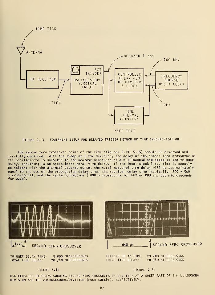
TIME TICK
V ANTENNADELAYED 1 pps
TOO kHz
o EXTTRIGGER
OSCILLOSCOPEVERTICALINPUT
TICK
CONTROLLEDDELAY GENOR DIVIDER
& CLOCK
TIMEINTERVALCOUNTER*
FREQUENCYSOURCE
OSC & CLOCK
1 pps
*STE TEXT
FIGURE 5.13. EQUIPMENT SETUP FOR DELAYED TRIGGER METHOD OF TIME SYNCHRONIZATION.
The second zero crossover point of the tick (figures 5-14, 5-15) should be observed and
carefully measured. With the sweep at 1 ms/ division, the delay of the second zero crossover on
the oscilloscope is measured to the nearest one-tenth of a millisecond and added to the triggerdelay, resulting in an approximate total time delay. If the local clock 1 pps time is exactlycoincident with the UTC(NBS) seconds pulse, the total measured time delay will be approximatelyequal to the sum of the propagation delay time, the receiver delay time (typically 200 - 500microseconds), and the cycle correction (1000 microseconds for WWV or CHU and 833 microsecondsfor WWVH).
IWI
SECOND ZERO CROSSOVER 540 ys SECOND ZERO CROSSOVER
TRIGGER DELAY TIME:
TOTAL TIME DELAY:19,000 MICROSECONDS20,7^0 MICROSECONDS
TRIGGER DELAY TIME:TOTAL TIME DELAY:
20,200 MICROSECONDS20,740 MICROSECONDS
FIGURE 5.14 FIGURE 5.15
OSCILLOSCOPE DISPLAYS SHOWING SECOND ZERO CROSSOVER OF WWV TICK AT A SWEEP RATE OF
DIVISION AND 100 MICROSECONDS/DIVISION (FOUR SWEEPS), RESPECTIVELY.
MILLISECOND/
87
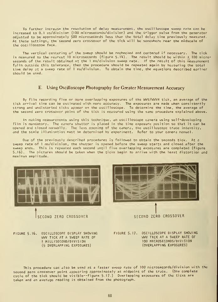
To further increase the resolution of delay measurement, the oscilloscope sweep rate can be
increased to 0.1 ms/division (100 microseconds/division) and the trigger pulse from the generatoradjusted to be approximately 500 microseconds less than the total delay time previously measured.
At these settings, the second zero crossover of the tick will be somewhere near the midscale of
the oscilloscope face.
The vertical centering of the sweep should be rechecked and centered if necessary. The tick
is measured to the nearest 10 microseconds (figure 5. 1*0. The result should be within + 100 micro-
seconds of the result obtained at the 1 ms/division sweep rate. If the result of this measurementfalls outside this tolerance, then the procedure should be repeated again by measuring the total
time delay at a sweep rate of 1 ms/division. To obtain the time, the equations described earliershould be used.
E. Using Oscilloscope Photography for Greater Measurement Accuracy
By film recording five or more overlapping exposures of the WWV/WWVH tick, an average of the
tick arrival time can be estimated with more accuracy. The exposures are made when consistentlystrong and undistorted ticks appear on the oscilloscope. To determine the time, the average of
the second zero crossover point of the tick is measured using the same procedure explained above.
In making measurements using this technique, an oscilloscope camera using self-developingfilm is mandatory. The camera shutter is placed in the time exposure position so that it can be
opened and closed manually. The lens opening of the camera, the oscilloscope trace intensity,and the scale illumination must be determined by experiment. Refer to your camera manual.
One of the previously described procedures is followed to obtain the seconds tick. At a
sweep rate of 1 ms/division, the shutter is opened before the sweep starts and closed after the
sweep ends. This is repeated each second until five overlapping exposures are completed (figure
5.16). The pictures should be taken when the ticks begin to arrive with the least distortion andmaximum amplitude.
inj^sss*
1
SECOND ZERO CROSSOVER SECOND ZERO CROSSOVER
FIGURE 5.16. OSCILLOSCOPE DISPLAY SHOWINGWWV TICK AT A SWEEP RATE OF
1 MILLISECOND/DIVISION
(5 OVERLAPPING EXPOSURES)
FIGURE 5.17. OSCILLOSCOPE DISPLAY SHOWING
WWV TICK AT A SWEEP RATE OF
100 MICROSECONDS/DIVISION(OVERLAPPING EXPOSURES)
This procedure can also be used at a faster sweep rate of 100 microseconds/division with the
second zero crossover point appearing approximately at midpoint of the trace. (One complete
cycle of the tick should be vi s
i
ble--f igure 5-17.) Overlapping exposures of the ticks are
taken and an average reading is obtained from the photograph.
88
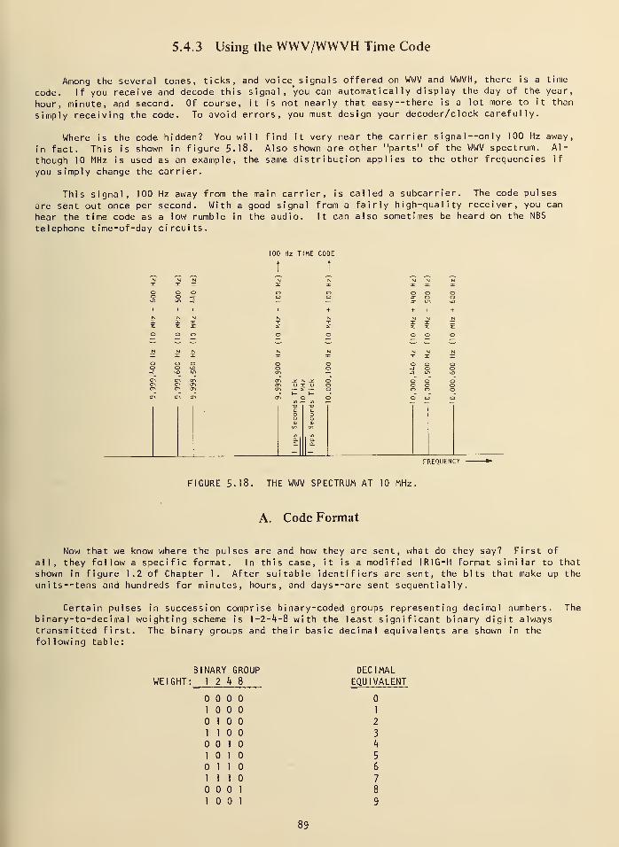
5.4.3 Using the WWV/WWVH Time Code
Among the several tones, ticks, and voice signals offered on WWV and WWVH, there is a time
code. If you receive and decode this signal, you can automatically display the day of the year,
hour, minute, and second. Of course, it is not nearly that easy-there is a lot more to it than
simply receiving the code. To avoid errors, you must design your decoder/clock carefully.
Where is the code hidden? You will find it very near the carrier signal—only 100 Hz away,
in fact. This is shown in figure 5.18. Also shown are other "parts" of the WWV spectrum. Al-
though 10 MHz is used as an example, the same distribution applies to the other frequencies if
you simply change the carrier.
This signal, 100 Hz away from the main carrier, is called a subcarrier. The code pulses
are sent out once per second. With a good signal from a fairly high-quality receiver, you can
hear the time code as a low rumble in the audio. It can also sometimes be heard on the NESS
telephone time-of-day circuits.
100 Hz TIME CODE
X)co
cOu
" <s>
Q. I
Dl1
°-Q.
—| 1
—FREQUENCY
FIGURE 5.18. THE WWV SPECTRUM AT 10 MHz.
A. Code Format
Now that we know where the pulses are and how they are sent, what do they say? First of
all, they follow a specific format. In this case, it is a modified IRIG-H format similar to that
shown in figure 1.2 of Chapter 1. After suitable identifiers are sent, the bits that make up the
units— tens and hundreds for minutes, hours, and days—are sent sequentially.
Certain pulses in succession comprise binary-coded groups representing decimal numbers. The
binary-to-decimal weighting scheme is 1-2-^-8 with the least significant binary digit alwaystransmitted first. The binary groups and their basic decimal equivalents are shown in thefollowing table:
BINARY GROUPWEIGHT: 12^8
1
1
1 1
1
1 1
1
1
1
1
1
1
1 1
DECIMALEQUIVALENT
1
2
3
h
5
6
7
89
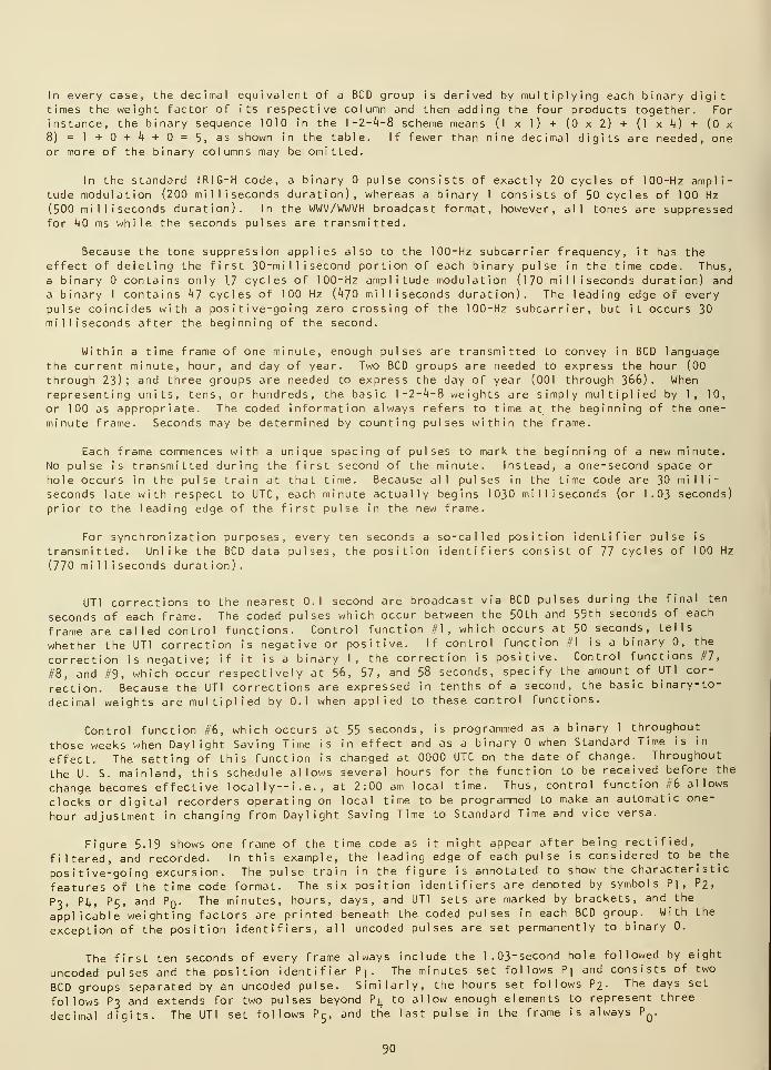
In every case, the decimal equivalent of a BCD group is derived by multiplying each binary digittimes the weight factor of its respective column and then adding the four products together. For
instance, the binary sequence 1010 in the 1-2-4-8 scheme means (1 x 1) + (0x2)+ (1 x 4) + (Ox8) = 1 + + 4 + = 5, as shown in the table. If fewer than nine decimal digits are needed, oneor more of the binary columns may be omitted.
In the standard IRIG-H code, a binary pulse consists of exactly 20 cycles of 100-Hz ampli-tude modulation (200 milliseconds duration), whereas a binary 1 consists of 50 cycles of 100 Hz
(500 milliseconds duration). In the WWV/WWVH broadcast format, however, all tones are suppressedfor 40 ms while the seconds pulses are transmitted.
Because the tone suppression applies also to the 100-Hz subcarrier frequency, it has theeffect of deleting the first 30-mi 1 1 i second portion of each binary pulse in the time code. Thus,
a binary contains only 1.7 cycles of 100-Hz amplitude modulation (170 milliseconds duration) anda binary 1 contains 47 cycles of 100 Hz (470 milliseconds duration). The leading edge of everypulse coincides with a positive-going zero crossing of the I 00-Hz subcarrier, but it occurs 30milliseconds after the beginning of the second.
Within a time frame of one minute, enough pulses are transmitted to convey in BCD language
the current minute, hour, and day of year. Two BCD groups are needed to express the hour (00
through 23); and three groups are needed to express the day of year (001 through 366). When
representing units, tens, or hundreds, the basic 1-2-4-8 weights are simply multiplied by 1, 10,
or 100 as appropriate. The coded information always refers to time at the beginning of the one-minute frame. Seconds may be determined by counting pulses within the frame.
Each frame commences with a unique spacing of pulses to mark the beginning of a new minute.No pulse is transmitted during the first second of the minute. Instead, a one-second space or
hole occurs in the pulse train at that time. Because all pulses in the time code are 30 milli-
seconds late with respect to UTC , each minute actually begins 1030 milliseconds (or 1.03 seconds)
prior to the leading edge of the first pulse in the new frame.
For synchronization purposes, every ten seconds a so-called position identifier pulse is
transmitted. Unlike the BCD data pulses, the position identifiers consist of 77 cycles of 100 Hz
(770 milliseconds duration).
UT1 corrections to the nearest 0.1 second are broadcast via BCD pulses during the final ten
seconds of each frame. The coded pulses which occur between the 50th and 59th seconds of each
frame are called control functions. Control function #1 , which occurs at 50 seconds, tells
whether the UT1 correction is negative or positive. If control function #1 is a binary 0, the
correction is negative; if it is a binary 1, the correction is positive. Control functions #7,
#8, and #9, which occur respectively at 56, 57, and 58 seconds, specify the amount of UTl cor-
rection. Because the UTl corrections are expressed in tenths of a second, the basic binary-to-
decimal weights are multiplied by 0.1 when applied to these control functions.
Control function #6, which occurs at 55 seconds, is programmed as a binary 1 throughout
those weeks when Daylight Saving Time is in effect and as a binary when Standard Time is in
effect. The setting of this function is changed at 0000 UTC on the date of change. Throughout
the U. S. mainland, this schedule allows several hours for the function to be received before the
change becomes effective local ly—i .e. , at 2:00 am local time. Thus, control function #6 allows
clocks or digital recorders operating on local time to be programmed to make an automatic one-
hour adjustment in changing from Daylight Saving Time to Standard Time and vice versa.
Figure 5.19 shows one frame of the time code as it might appear after being rectified,
filtered, and recorded. In this example, the leading edge of each pulse is considered to be the
positive-going excursion. The pulse train in the figure is annotated to show the characteristic
features of the time code format. The six position identifiers are denoted by symbols Pi, P2,
P3, P2j, P5, and P - The minutes, hours, days, and UTl sets are marked by brackets, and the
applicable weighting factors are printed beneath the coded pulses in each BCD group. With the
exception of the position identifiers, all uncoded pulses are set permanently to binary 0.
The first ten seconds of every frame always include the 1.03"Second hole followed by eight
uncoded pulses and the position identifier P]. The minutes set follows Pi and consists of two
BCD groups separated by an uncoded pulse. Similarly, the hours set follows P2- The days set
follows P3 and extends for two pulses beyond P ^ to allow enough elements to represent three
decimal digits. The UTl set follows P5, and the last pulse in the frame is always PQ
.
90
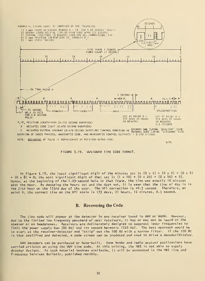
FORMAT H, SIGNAL HOOl , IS COMPOSED OF THE FOLLOWING
1) 1 ppm FRAME REFERENCE MARKER R = ( P „ AND 1.03 SECOND "HOLE")2) BINARY CODED DECIMAL TIME-OF-YEAR CODE WORD (23 DIGITS)
CONTROL FUNCTIONS (9 DIGITS) USED FOR UT! CORRECTIONS, ETC.6 ppm POSITION IDENTIFIERS (P THROUGH P
1 pps INDEX MARKERS 5
t <— 1 .03 SECONDR-l HOLE IN CODE
FOR 0.8 SECONDPULSE
-MINUTES- -HOURS
P -PsPOSITION IDENTIFIERS (0.770 SECOND DURATION)
W WEIGHTED CODE DIGIT (0.470 SECOND DURATION)
UTC AT POINT A =
173 DAYS 21 HOURS10 MINUTES
UTiCORRECTION
UT1 AT POINT A =
173 DAYS 21 HOURS10 MINUTES0.3 SECONDS
(BINARY ONE DURING DAYLIGHT TIME(BINARY ZERO DURING 'STANDARD' TIME
DURATION OF INDEX MARKERS, UNWEIGHTED CODE, AND UNWEIGHTED CONTROL ELEMENTS = 0.170 SECONDS
WEIGHTED CONTROL ELEMENT (0.470 SECOND DURATION) CONTROL FUNCTION #6
NOTE: BEGINNING OF PULSE IS REPRESENTED BY POSITIVE-GOING EDGE.
9/75
FIGURE 5.19. WWV/WWVH TIME CODE FORMAT.
In figure 5.19, the least significant digit of the minutes set is (0 x 1 ) + (0 x 2) + (0 x 4)
+ (0 x 8) = 0; the most significant digit of that set is (1 x 10) + (0 x 20) + (0 x *tO) = 10.
Hence, at the beginning of the 1.03-second hole in that frame, the time was exactly 10 minutes
past the hour. By decoding the hours set and the days set, it is seen that the time of day is in
the 21st hour on the 173rd day of the year. The UT1 correction is +0.3 second. Therefore, at
point A, the correct time on the UT1 scale is 173 days, 21 hours, 10 minutes, 0.3 second.
B. Recovering the Code
The time code will appear at the detector in any receiver tuned to WWV or WWVH. However,
due to the limited low frequency passband of most receivers, it may or may not be heard at the
speaker or on headphones. Receivers are deliberately designed to suppress lower frequencies to
limit the power supply hum (60 Hz) and its second harmonic (120 Hz). The best approach would be
to start at the receiver-detector and "strip" out the 100 Hz with a narrow filter. If the 100 Hz
is then amplified and detected, a code stream can be produced and used to drive a decoder/display,
WWV decoders can be purchased or home-built. Some hobby and radio amateur publications have
carried articles on using the WWV time code. At this writing, the NBS is not able to supply
decoder designs. As such material becomes available, it will be announced in the NBS Time and
Frequency Services Bulletin, published monthly.
91
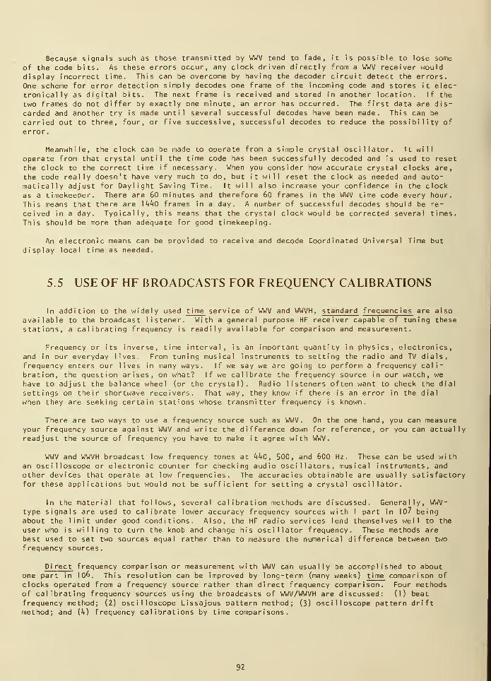
Because signals such as those transmitted by WWV tend to fade, it is possible to lose some
of the code bits. As these errors occur, any clock driven directly from a WWV receiver would
display incorrect time. This can be overcome by having the decoder circuit detect the errors.
One scheme for error detection simply decodes one frame of the incoming code and stores it elec-tronically as digital bits. The next frame is received and stored in another location. If the
two frames do not differ by exactly one minute, an error has occurred. The first data are dis-
carded and another try is made until several successful decodes have been made. This can be
carried out to three, four, or five successive, successful decodes to reduce the possibility of
error.
Meanwhile, the clock can be made to operate from a simple crystal oscillator. It will
operate from that crystal until the time code has been successfully decoded and is used to reset
the clock to the correct time if necessary. When you consider how accurate crystal clocks are,
the code really doesn't have very much to do, but it will reset the clock as needed and auto-matically adjust for Daylight Saving Time. It will also increase your confidence in the clock
as a timekeeper. There are 60 minutes and therefore 60 frames in the WWV time code every hour.
This means that there are ]kk0 frames in a day. A number of successful decodes should be re-
ceived in a day. Typically, this means that the crystal clock would be corrected several times.
This should be more than adequate for good timekeeping.
An electronic means can be provided to receive and decode Coordinated Universal Time but
display local time as needed.
5.5 USE OF HF BROADCASTS FOR FREQUENCY CALIBRATIONS
In addition to the widely used t ime service of WWV and WWVH, standard frequencies are also
available to the broadcast listener. With a general purpose HF receiver capable of tuning these
stations, a calibrating frequency is readily available for comparison and measurement.
Frequency or its inverse, time interval, is an important quantity in physics, electronics,and in our everyday lives. From tuning musical instruments to setting the radio and TV dials,
frequency enters our lives in many ways. If we say we are going to perform a frequency cali-
bration, the question arises, on what? If we calibrate the frequency source in our watch, we
have to adjust the balance wheel (or the crystal). Radio listeners often want to check the dial
settings on their shortwave receivers. That way, they know if there is an error in the dial
when they are seeking certain stations whose transmitter frequency is known.
There are two ways to use a frequency source such as WWV. On the one hand, you can measureyour frequency source against WWV and write the difference down for reference, or you can actuallyreadjust the source of frequency you have to make it agree with WWV.
WWV and WWVH broadcast low frequency tones at kkO , 500, and 600 Hz. These can be used withan oscilloscope or electronic counter for checking audio oscillators, musical instruments, and
other devices that operate at low frequencies. The accuracies obtainable are usually satisfactoryfor these applications but would not be sufficient for setting a crystal oscillator.
In the material that follows, several calibration methods are discussed. Generally, WWV-type signals are used to calibrate lower accuracy frequency sources with 1 part in 1 7 beingabout the limit under good conditions. Also, the HF radio services lend themselves well to the
user who is willing to turn the knob and change his oscillator frequency. These methods arebest used to set two sources equal rather than to measure the numerical difference between two
frequency sources.
Pi rect frequency comparison or measurement with WWV can usually be accomplished to aboutone part in 106. This resolution can be improved by long-term (many weeks) time comparison of
clocks operated from a frequency source rather than direct frequency comparison. Four methodsof calibrating frequency sources using the broadcasts of WWV/WWVH are discussed: (1) beat
frequency method; (2) oscilloscope Lissajous pattern method; (3) oscilloscope pattern driftmethod; and (k) frequency calibrations by time comparisons.
92
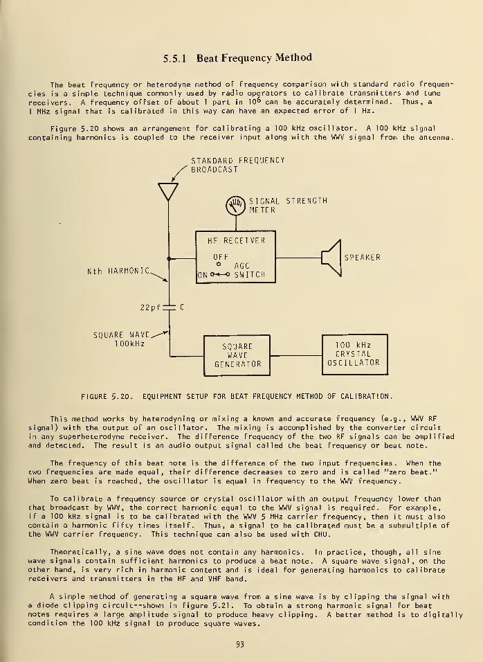
5.5.1 Beat Frequency Method
The beat frequency or heterodyne method of frequency comparison with standard radio frequen-
cies is a simple technique commonly used by radio operators to calibrate transmitters and tune
receivers. A frequency offset of about 1 part in 10° can be accurately determined. Thus, a
1 MHz signal that is calibrated in this way can have an expected error of 1 Hz.
Figure 5.20 shows an arrangement for calibrating a 100 kHz oscillator. A 100 kHz signal
containing harmonics is coupled to the receiver input along with the WWV signal from the antenna.
STANDARD FREQUENCYBROADCAST
V
Nth HARMONIC.
22pf .
SIGNAL STRENGTHMETER
HF RECEIVER
OFF° AGC
ON o-.-o SWITCH
SQUARE WAVE.1 00kHz
< SPEAKER
SQUAREWAVE
GENERATOR
100 kHzCRYSTAL
OSCILLATOR
FIGURE 5.20. EQUIPMENT SETUP FOR BEAT FREQUENCY METHOD OF CALIBRATION.
This method works by heterodyning or mixing a known and accurate frequency (e.g., WWV RF
signal) with the output of an oscillator. The mixing is accomplished by the converter circuitin any superheterodyne receiver. The difference frequency of the two RF signals can be amplifiedand detected. The result is an audio output signal called the beat frequency or beat note.
The frequency of this beat note is the difference of the two input frequencies. When the
two frequencies are made equal, their difference decreases to zero and is called "zero beat."When zero beat is reached, the oscillator is equal in frequency to the WWV frequency.
To calibrate a frequency source or crystal oscillator with an output frequency lower thanthat broadcast by WWV, the correct harmonic equal to the WWV signal is required. For example,if a 100 kHz signal is to be calibrated with the WWV 5 MHz carrier frequency, then it must alsocontain a harmonic fifty times itself. Thus, a signal to be calibrated must be a submultiple ofthe WWV carrier frequency. This technique can also be used with CHU.
Theoretically, a sine wave does not contain any harmonics. In practice, though, all sinewave signals contain sufficient harmonics to produce a beat note. A square wave signal, on theother hand, is very rich in harmonic content and is ideal for generating harmonics to calibratereceivers and transmitters in the HF and VHF band.
A simple method of generating a square wave from a sine wave is by clipping the signal witha diode clipping ci rcui t--shown in figure 5.21. To obtain a strong harmonic signal for beatnotes requires a large amplitude signal to produce heavy clipping. A better method is to digitallycondition the 100 kHz signal to produce square waves.
93
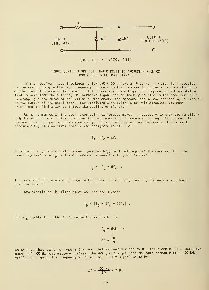
INPUT(SINE WAVE
OUTPUT(SQUARE WAVE)
CR1 , CR2 = IN270, 1N34
FIGURE 5.21 DIODE CLIPPING CIRCUIT TO PRODUCE HARMONICSFROM A PURE SINE WAVE SIGNAL.
If the receiver input impedance is low (50 -100 ohms), a 10 to 20 picofarad (pf) capacitorcan be used to couple the high frequency harmonic to the receiver input and to reduce the level
of the lower fundamental frequency. If the receiver has a high input impedance with unshieldedlead-in wire from the antenna, the harmonic signal can be loosely coupled to the receiver input
by wrapping a few turns of an insulated wire around the antenna lead-in and connecting it directlyto the output of the oscillator. For receivers with built-in or whip antennas, you mustexperiment to find a way to inject the oscillator signal.
Using harmonics of the oscillator being calibrated makes it necessary to know the relation-ship between the oscillator error and the beat note that is measured during calibration. Let
the oscillator output be designated as fp. This is made up of two components, the correctfrequency fg, plus an error that we can designate as Af. So:
fF
= fQ
+ Af.
A harmonic of this oscillator signal (written Nfp
) will beat against the carrier, f . The
resulting beat note f is the difference between the two, written as:D
fB
= fc
- Nfp |
The bars mean that a negative sign in the answer is ignored; that is, the answer is always a
positive number.
Now substitute the first equation into the second:
fB
= |fc
- NfQ
- NAfp
|.
But Nf„ equals f . That's why we multiplied by N. So:
f. = NAf, orD
Af =N
'
which says that the error equals the beat that we hear divided by N. For example, if a beat fre-
quency of 100 Hz were measured between the WWV 5 MHz signal and the 50th harmonic of a 100 kHz
oscillator signal, the frequency error of the 100 kHz signal would be:
Af100 Hz
50
94
= 2 Hz.
The oscillator frequency is in error by 2 Hz. To determine whether the oscillator is highor low in frequency, the oscillator frequency has to be changed to note which way the beat fre-quency decreases. I f ,i ncreas ing the oscillator frequency decreases the beat note, it indicatesthat the oscillator frequency is lower than the WWV/WWVH frequency.
In a receiver with no tuned RF amplifier between the mixer stage and the antenna input, a
low frequency sine wave signal can enter the mixer stage directly and generate unwanted harmonicsand confusing beat notes due to the nonlinear characteristics of a mixer circuit. However, a
good communications receiver or a specia 1 -purpose WWV receiver generally has tuned RF amplifierstages or preselectors before its first mixer stage. Then, only the desired beat note from two
input signals is produced.
If the beat note is above 50 Hz, headphones, a speaker, or a counter can be used. Belowthat frequency, a dc oscilloscope can be connected to the receiver detector. A signal strengthmeter can be used and the beats counted visually. The automatic gain control (AGC) should be
disabled, if possible, for the meter fluctuations to be more noticeable. The manual RF gain canbe adjusted to compensate for loss of the AGC.
To correct the oscillator frequency, the adjustment knob is turned in the direction whichlowers the frequency of the beat note. Between 50 Hz and about 1 Hz, the beat note cannot be
heard and the signal strength meter will begin to respond to the beat note as it approaches 1
Hz. As zero beat is approached, a very slow rise and fall of the background noise or the WWVaudio tone can also be heard on the speaker. The meter effect is much easier to follow. As it
approaches zero beat, the very slow rise and fall of the signal strength may sometimes becomedifficult to distinguish from signal fading due to propagation effects.
To overcome fading effects, the oscillator adjustment can be interpolated. First, adjustthe oscillator to a minimum beat frequency that can be measured without interference. For
accuracy, count the number of deflections of the signal strength meter in 10 seconds. Thesetting of the frequency adjustment is then marked. The adjustment is then made to pass zerobeat until the beat is again visible on the meter. By obtaining the same number of meterdeflections as the previous beat note, the frequency can be set midway between the two
adjustments
.
The frequency of crystal oscillators changes with time. This is commonly referred to as
the aging or drift rate. Therefore, all crystal oscillators must be recalibrated periodicallyif maximum accuracy is desired.
5.5.2 Oscilloscope Lissajous Pattern Method
Audio oscillators can be calibrated by using WWV/WWVH audio tones to produce Lissajous
patterns on an oscilloscope. Lissajous patterns are fully discussed in Chapter k. The WWV
audio signal is applied to the vertical input of the scope and the oscillator signal to be
calibrated is used to drive the horizontal amplifier. The resultant pattern tells the user two
things: (1) the frequency ratio between his oscillator setting and the received tone, and (2)
movement of the oscillator relative to WWV.
The tones available on WWV nd WWVH are mainly 500 and 600 Hz. CHU transmits 1 kHz ticks
that last for about one-third second. If these are used, they will produce an oscilloscopepattern at the tick rate; i.e., once per second. Even the WWV/WWVH ticks can be used this way.
Most important, the user should be aware of the exact format being broadcast to avoid making
errors. This can be a problem because WWV and WWVH switch between 500 and 600 Hz in alternateminutes and the kkO Hz is used for only one minute every hour.
95
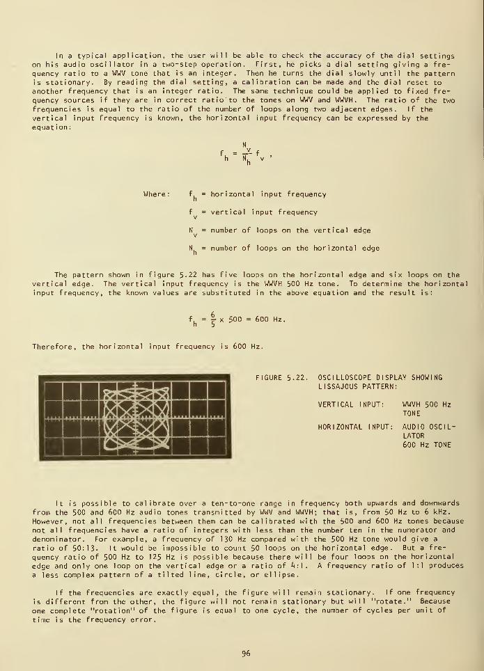
In a typical application, the user will be able to check the accuracy of the dial settingson his audio oscillator in a two-step operation. First, he picks a dial setting giving a fre-
quency ratio to a WWV tone that is an integer. Then he turns the dial slowly until the patternis stationary. By reading the dial setting, a calibration can be made and the dial reset to
another frequency that is an integer ratio. The same technique could be applied to fixed fre-
sncy sources if they are in correct ratio to the tones on WWV and WWVH. The ratio of the twoquer*-| uci I i- y D wu I i_c D II Lucy a i ^ ill \_w i i <^'_ l i o l i '~. ii~/ tnc lui icj uii rirvv anu nnmi , I lie I a L 1 U Ul Lilt
frequencies is equal to the ratio of the number of loops along two adjacent edges. If the
vertical input frequency is known, the horizontal input frequency can be expressed by the
equat ion:
f = — fh N, v
n
Where: f = horizontal input frequency
f = vertical input frequency
N = number of loops on the vertical edgev
N = number of loops on the horizontal edge
The pattern shown in figure 5.22 has five loops on the horizontal edge and six loops on the
vertical edge. The vertical input frequency is the WWVH 500 Hz tone. To determine the horizontalinput frequency, the known values are substituted in the above equation and the result is:
f, = |- x 500 = 600 Hz.
Therefore, the horizontal input frequency is 600 Hz.
FIGURE 5.22. OSCILLOSCOPE DISPLAY SHOWINGLISSAJ0US PATTERN:
VERTICAL INPUT: WWVH 500 Hz
TONE
HORIZONTAL INPUT: AUDIO OSCIL-
LATOR600 Hz TONE
It is possible to calibrate over a ten-to-one range in frequency both upwards and downwards
from the 500 and 600 Hz audio tones transmitted by WWV and WWVH; that is, from 50 Hz to 6 kHz.
However, not all frequencies between them can be calibrated with the 500 and 600 Hz tones because
not all frequencies have a ratio of integers with less than the number ten in the numerator and
denominator. For example, a frequency of 130 Hz compared with the 500 Hz tone would give a
ratio of 50:13. It would be impossible to count 50 loops on the horizontal edge. But a fre-
quency ratio of 500 Hz to 125 Hz is possible because there will be four loops on the horizontal
edge and only one loop on the vertical edge or a ratio of k:]. A frequency ratio of 1 : 1 produces
a less complex pattern of a tilted line, circle, or ellipse.
If the frequencies are exactly equal, the figure will remain stationary. If one frequency
is different from the other, the figure will not remain stationary but will "rotate." Because
one complete "rotation" of the figure is equal to one cycle, the number of cycles per unit of
time is the frequency error.
96
For example : If a Lissajous figure takes ten seconds to "rotate" through one cycle and the
frequency being compared is 600 Hz, the frequency error is:
Af = T= To='
- 1 Hz
r D 1 _• r Af 0.1 . t . n~kF = Relative Frequency = —j = yjrz- = 1./ x 10
Since the error is inversely proportional to the time it takes to complete one cycle, it is
obvious that the longer it takes to complete a cycle, the smaller the error will be.
The accuracy of measurement of a Lissajous pattern by the comparison method described aboveis inversely proportional to the frequency. For example, if the time required for a Lissajousfigure to "rotate" through one cycle is ten seconds at a frequency of 1 MHz:
r d i <-• c Af 0. 1 Hz . .--7F = Relative Frequency = —= = 7 = 1 x 10
1 x 10 Hz
If, instead of measuring at 1 MHz, we observe the Lissajous pattern at 1 kHz:
Af = f x F = 1 x 103
x 1 x 10" 7 = 10 Hz
and the observation time would be:
J_Af
10X = 10,000 seconds,
Thus, it would take too long to measure signals with relative frequencies of less than 1 x 10
at 1 kHz. A more accurate method which measures the phase shift on an oscilloscope will be
discussed next.
5
5.5.3 Oscilloscope Pattern Drift Method
The oscilloscope pattern drift method is good for comparing two frequencies if you have an
oscilloscope with external triggering. It can detect smaller frequency differences than the
Lissajous pattern at audio frequencies.
The method consists of an oscilloscope with an accurately calibrated sweep time base.
External triggering is obtained from the signal to be calibrated. This signal can be any integersubmultiple of the tone being received from WWV/WWVH. The receiver (tuned to WWV) has its audiooutput connected to the vertical input of the oscilloscope. With the sweep rate set at 1 milli-second/division, the trigger level is adjusted so that a zero crossover of the corresponding 600or 500 Hz signal is near midscale on the scope.
By measuring the phase drift during a given time interval, the frequency error is deter-mined. If the zero crossover moves to the right, the audio signal frequency is higher than theWWV signal, and if it moves to the left, the signal is lower in frequency (fig. 5 - 23 ) •
For example, if during a count of 10 seconds at 500 Hz, the zero crossover advanced fromleft to right by 0.1 millisecond, the relative frequency is:
c phase d r ift +0.1 x 10 ,. ,_-5F = -*r r—
7
r = TK =+1x10 ,time interval 10
97
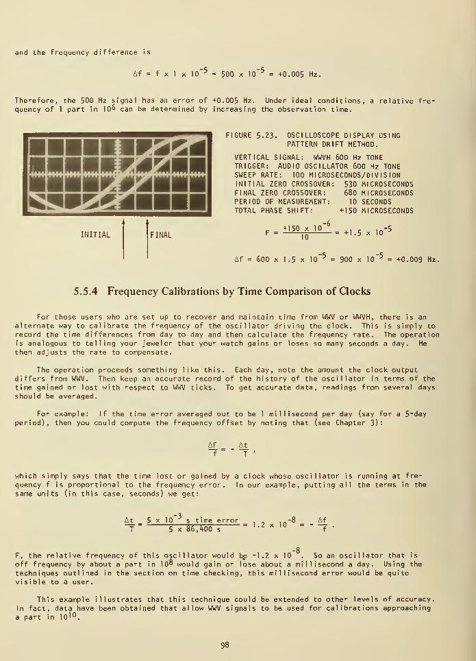
and the frequency difference is
Af = f x 1 x 10" 5 = 500 x 10"5 = +0.005 Hz.
Therefore, the 500 Hz signal has an error of +0.005 Hz. Under ideal conditions, a relative fre-
quency of 1 part in 10° can be determined by increasing the observation time.
FIGURE 5-23. OSCILLOSCOPE DISPLAY USINGPATTERN DRIFT METHOD.
VERTICAL SIGNAL: WWVH 600 Hz TONETRIGGER: AUDIO OSCILLATOR 600 Hz TONESWEEP RATE: 100 MICROSECONDS/DIVISIONINITIAL ZERO CROSSOVER: 530 MICROSECONDSFINAL ZERO CROSSOVER: 680 MICROSECONDSPERIOD OF MEASUREMENT: 10 SECONDSTOTAL PHASE SHIFT: +150 MICROSECONDS
F = +150 x 10
10
-6
= +1 .5 x 10-5
Af = 600 x 1 .5 x 105 = 900 x 10" 5
= +0.009 Hz,
5.5.4 Frequency Calibrations by Time Comparison of Clocks
For those users who are set up to recover and maintain time from WWV or WWVH, there is an
alternate way to calibrate the frequency of the oscillator driving the clock. This is simply to
record the time differences from day to day and then calculate the frequency rate. The operationis analogous to telling your jeweler that your watch gains or loses so many seconds a day. He
then adjusts the rate to compensate.
The operation proceeds something like this. Each day, note the amount the clock outputdiffers from WWV. Then keep an accurate record of the history of the oscillator in terms of the
time gained or lost with respect to WWV ticks. To get accurate data, readings from several daysshould be averaged.
For example: If the time error averaged out to be 1 millisecond per day (say for a 5-day
period), then you could compute the frequency offset by noting that (see Chapter 3):
Af
f
A_t_
T
which simply says that the time lost or gained by a clock whose oscillator is running at fre-
quency f is proportional to the frequency error. In our example, putting all the terms in the
same units (in this case, seconds) we get:
A_t_
T5 x 10
3s time error
5 x 86,400 s= 1.2 x 10
Af
f
F, the relative frequency of this oscillator would be -1.2 x 10 . So an oscillator that is
off frequency by about a part in 10° would gain or lose about a millisecond a day. Using the
techniques outlined in the section on time checking, this millisecond error would be quitevisible to a user.
This example illustrates that this technique could be extended to other levels of accuracy.
In fact, data have been obtained that allow WWV signals to be used for calibrations approachinga part in 10 10 .
98
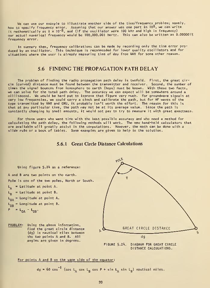
We can use our example to illustrate another side of the time/frequency problem; namely,
how to specify frequency error. Assuming that our answer was one part in 10°, we can write
it mathematically as 1 x 10_°\ and (if the oscillator were 100 kHz and high in frequency)
our actual numerical frequency would be 100,000.001 hertz. This can also be written as 0.000001%
frequency error.
In summary then, frequency calibrations can be made by recording only the time error pro-
duced by an oscillator. This technique is recommended for lower quality oscillators and for
situations where the user is already measuring time of day from WWV for some other reason.
5.6 FINDING THE PROPAGATION PATH DELAY
The problem of finding the radio propagation path delay is twofold. First, the great cir-
cle (curved) distance must be found between the transmitter and receiver. Second, the number of
times the signal bounces from ionosphere to earth (hops) must be known. With these two facts,
we can solve for the total path delay. The accuracy we can expect will be somewhere around a
millisecond. We would be hard put to improve that figure very much. For groundwave signals at
very low frequencies, we could carry a clock and calibrate the path, but for HF waves of the
type transmitted by WWV and CHU, it probably isn't worth the effort. The reason for this is
that at any particular time, the path may not be at its average value. Since the path is
constantly changing by small amounts, it would not pay to try to measure it with great exactness.
For those users who want time with the best possible accuracy and who need a method for
calculating the path delay, the following methods will work. The new hand-held calculators that
are available will greatly assist in the computations. However, the math can be done with a
slide rule or a book of tables. Some examples are given to help in the solution.
5.6. 1 Great Circle Distance Calculations
Using figure 5.24 as a reference:
A and B are two points on the earth.
Pole is one of the two poles, North or South.
L. = Latitude at point A.
L D = Latitude at point B.D
L_. = Longitude at point A.
L_ D = Longitude at point B.(Jb
P = L - L .
0A 0B
PROBLEM : Using the above information,find the great circle distance(dg) in nautical miles betweenthe two points A and B. All
angles are given in degrees.FIGURE 5.24. DIAGRAM FOR GREAT CIRCLE
DISTANCE CALCULATIONS.
For points A and B on the same side of the equator :
dg = 60 cos (cos L. cos LR
cos P + sin L. sin LR
) nautical miles,
99
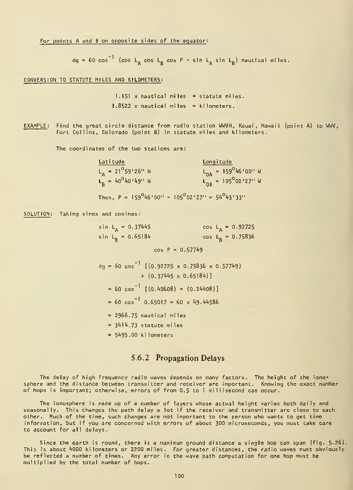
For points A and B on opposite sides of the equator :
dg = 60 cos (cos L. cos L„ cos P - sin L. sin L D ) nautical miles.A d Ab
CONVERSION TO STATUTE MILES AND KILOMETERS :
1.151 x nautical miles = statute miles.
1.8522 x nautical miles = kilometers.
EXAMPLE : Find the great circle distance from radio station WWVH, Kauai, Hawaii (point A) to WWV
,
Fort Collins, Colorado (point B) in statute miles and kilometers.
The coordinates of the two stations are:
Lati tude Longi tude
Lft
= 21°59'26" N LQA
= 159°46'00" W
L D = 40°40'49" N LnD = 105°02'27" WD Ub
Then, P = 159°^6
'00" - 105°02'27" = 54°43'33"
SOLUTION : Taking sines and cosines:
sin LA
= 0.37445 cos LA
= 0.92725
sin L D = 0.65184 cos L D = O.75836O D
cos P = 0. 577*49
dg = 60 cos"1
[(0.92725 x 0.75836 x 0.57749)
+ (0.37445 x 0.65184)]
= 60 cos"' [(0.40608) + (0.24408)]
= 60 cos"1
0.65017 = 60 x 49.44586
= 2966.75 nautical miles
= 3414.73 statute mi les
= 5495.00 ki lometers
5.6.2 Propagation Delays
The delay of high frequency radio waves depends on many factors. The height of the iono-sphere and the distance between transmitter and receiver are important. Knowing the exact numberof hops is important; otherwise, errors of from 0.5 to 1 millisecond can occur.
The ionosphere is made up of a number of layers whose actual height varies both daily and
seasonally. This changes the path delay a lot if the receiver and transmitter are close to each
other. Much of the time, such changes are not important to the person who wants to get time
information, but if you are concerned with errors of about 300 microseconds, you must take care
to account for all delays.
Since the earth is round, there is a maximum ground distance a single hop can span (fig. 5-26),
This is about 4000 kilometers or 2200 miles. For greater distances, the radio waves must obviouslybe reflected a number of times. Any error in the wave path computation for one hop must be
multiplied by the total number of hops.
100
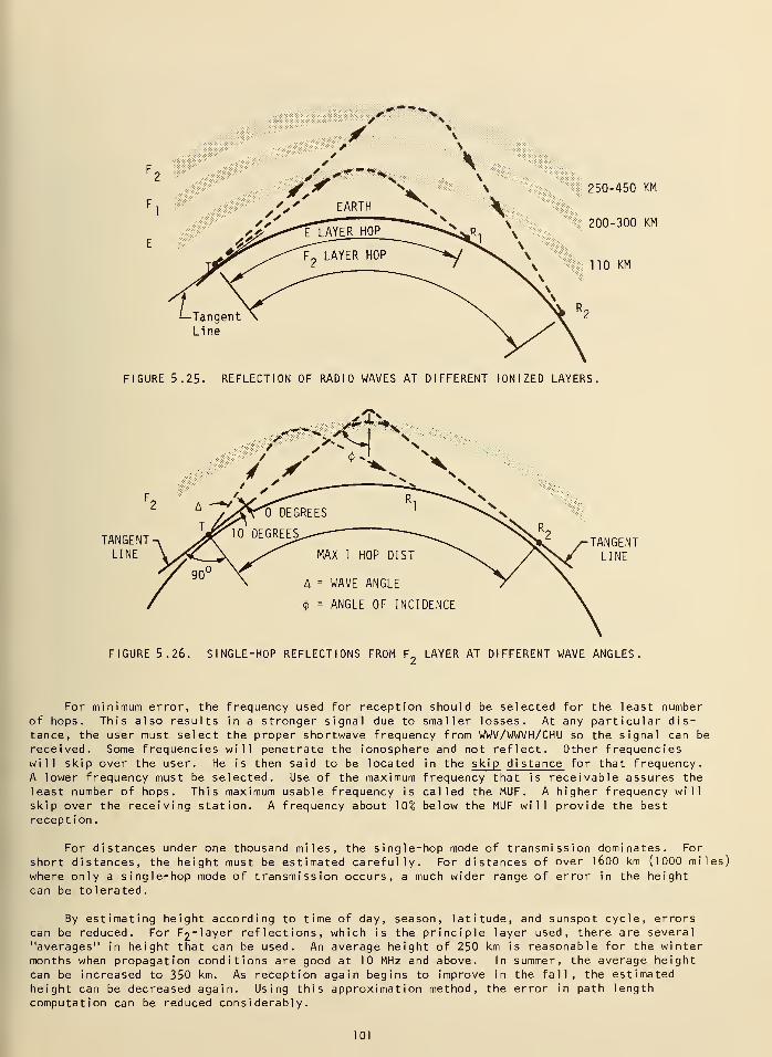
250-450 KM
200-300 KM
110 KM
igen
Line
FIGURE 5.25. REFLECTION OF RADIO WAVES AT DIFFERENT IONIZED LAYERS
TANGENTLINE
TANGENTLINE
FIGURE 5.26. SINGLE-HOP REFLECTIONS FROM F2
LAYER AT DIFFERENT WAVE ANGLES.
For minimum error, the frequency used for reception should be selected for the least numberof hops. This also results in a stronger signal due to smaller losses. At any particular dis-tance, the user must select the proper shortwave frequency from WWV/WWVH/CHU so the signal can be
received. Some frequencies will penetrate the ionosphere and not reflect. Other frequencieswill skip over the user. He is then said to be located in the skip distance for that frequency.A lower frequency must be selected. Use of the maximum frequency that is receivable assures theleast number of hops. This maximum usable frequency is called the MUF. A higher frequency will
skip over the receiving station. A frequency about 10% below the MUF will provide the best
recept ion.
For distances under one thousand miles, the single-hop mode of transmission dominates. For
short distances, the height must be estimated carefully. For distances of over 1 600 km (1000 miles)
where only a single-hop mode of transmission occurs, a much wider range of error in the heightcan be tolerated.
By estimating height according to time of day, season, latitude, and sunspot cycle, errorscan be reduced. For F2 _ layer reflections, which is the principle layer used, there are several
"averages" in height that can be used. An average height of 250 km is reasonable for the wintermonths when propagation conditions are good at 10 MHz and above. In summer, the average height
can be increased to 350 km. As reception again begins to improve in the fall, the estimatedheight can be decreased again. Using this approximation method, the error in path length
computation can be reduced considerably.
101
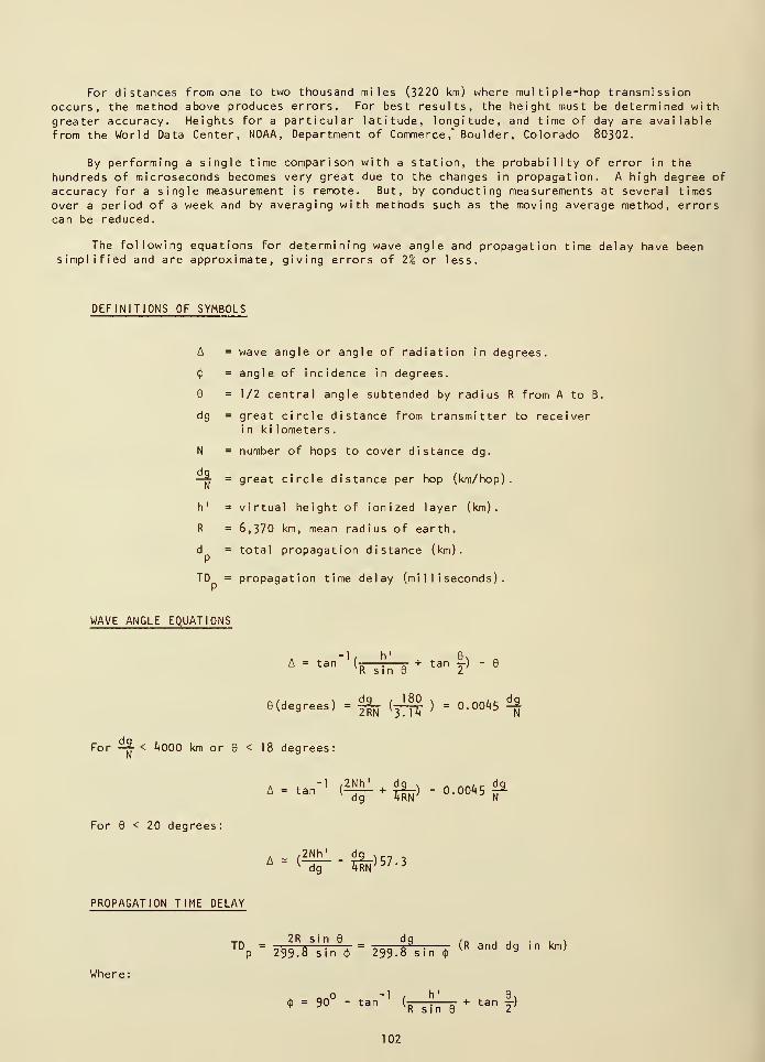
For distances from one to two thousand miles (3220 km) where multiple-hop transmissionoccurs, the method above produces errors. For best results, the height must be determined with
greater accuracy. Heights for a particular latitude, longitude, and time of day are availablefrom the World Data Center, NOAA, Department of Commerce," Boulder, Colorado 80302.
By performing a single time comparison with a station, the probability of error in the
hundreds of microseconds becomes very great due to the changes in propagation. A high degree of
accuracy for a single measurement is remote. But, by conducting measurements at several times
over a period of a week and by averaging with methods such as the moving average method, errorscan be reduced.
The following equations for determining wave angle and propagation time delay have beensimplified and are approximate, giving errors of 2% or less.
DEFINITIONS OF SYMBOLS
A = wave angle or angle of radiation in degrees.
(J)= angle of incidence in degrees.
6 = 1/2 central angle subtended by radius R from A to B.
dg = great circle distance from transmitter to receiverin ki lometers
.
N = number of hops to cover distance dg.
—jjj-= great circle distance per hop (km/hop).
h' = virtual height of ionized layer (km).
R = 6,370 km, mean radius of earth,
d = total propagation distance (km).
TD = propagation time delay (milliseconds).
WAVE ANGLE EQUATIONS
A = tan~1(fTsTn-T
+ tan I} "
e(degrees) = fa(Jl°
) = 0.00*5 *[
For -S. < 4000 km or 6 < 18 degrees:
For < 20 degrees:
PROPAGATION TIME DELAY
»-«""' <TT &> " "-a*'
S
1
,2Nh' dgN__ .A= (-di-"w 57 - 3
Where:
-itn 2R sin 9 dg /„ . . . . \
TD = _..- a : r = „__ 6J
. t- (R and dg in km)p 299.0 sin <p 299-8 sin cp
= 9°°- tan"
1
<RimT +tan £>
102
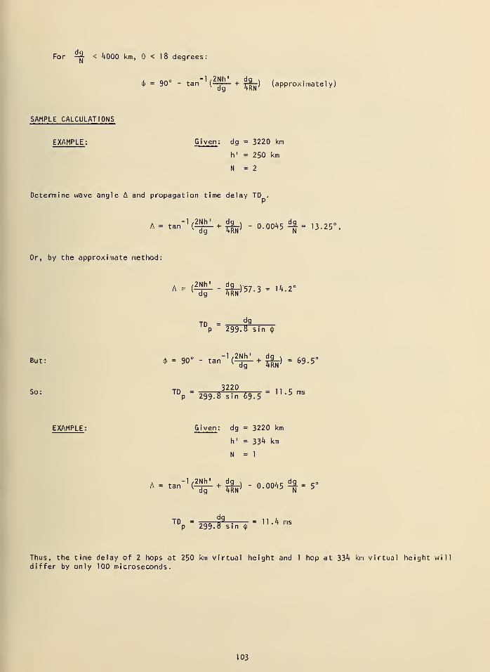
For -9- < 4000 km, 9 < 18 degrees:
(j) = 90° - tan (-jT- +
Tj^j")(approximately)
SAMPLE CALCULATIONS
EXAMPLE : Given : dg = 3220 km
h' =250 km
N = 2
Determine wave angle A and propagation time delay TD .
A - tan_1 <Tr + fe -0.00.5^=13.25%
Or, by the approximate method:
,2Nh' d
dgTD =
p 299.8 sin
* -SO- tan"1
(^Jfc)- 69.5-
So:3220 .. _
TDP
=299-8 sin 69.5
= 1K5 mS
EXAMPLE : Given : dg = 3220 km
h1 =33^ km
N = 1
*=«""<Tf*fe-»*!-''
p 299-0 sin <p
Thus, the time delay of 2 hops at 250 km virtual height and 1 hop at 33. km virtual height willdiffer by only 100 microseconds.
103
5.7 THE NBS TELEPHONE TIME-OF-DAY SERVICE
For those users who cannnot set up a shortwave receiver for WWV or who have other diffi-culties, NBS operates a telephone time-of-day service. Anyone who dials (303) ^+39 — 7111 will
hear the very same signals that are broadcast over WWV. The machines at Ft. Collins, Colorado,which generate the WWV format, are connected via telephone lines to a room in the BoulderLaboratories where the telephone equipment is maintained.
This telephone service is widely used, both in the local Denver calling area and via longdistance. The telephone service can handle eight incoming calls simultaneously. In addition,four lines are available through the government switchboard at Boulder for use by other govern-ment agencies. These are on FTS number 323-^2^5, h2kG , klkl , and klk%
.
The actual time you hear on the telephone will differ by a few milliseconds from that heardover WWV via radio. This is because of the delay in the telephone lines. In addition, if youare calling from any great distance, the way in which the telephone company handles your call
limits the total accuracy of the WWV tone to a few hertz. This means that if you are trying to
make a calibration at 1000 hertz, you could have an error as great as three cycles per second.This accuracy is not as good as that which can be achieved using radio methods. Users arewarned about this limit of accuracy over the telephone.
Because the telephone service is very often fully utilized, you may get a busy signal. If
this happens, wait a few minutes and redial. After your call is connected, the system willautomatically hang up in three minutes unless you hang up first.
5.8 SUMMARY
As stated early in this chapter, HF radio broadcasts are commonly used for time and fre-quency calibrations. Accuracies ranging from 1 ms for time-of-day to 1 part in 107 for fre-quency can be obtained. The NBS telephone time-of-day service can also be used when accuracyrequirements are not critical. However, if your requirements are higher, you should probablyuse one of the other methods discussed in the following chapters.
104
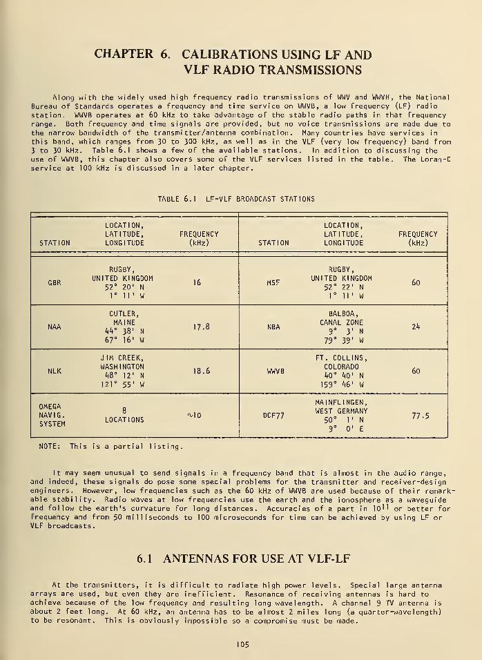
CHAPTER 6. CALIBRATIONS USING LF ANDVLF RADIO TRANSMISSIONS
Along with the widely used high frequency radio transmissions of WWV and WWVH , the National
Bureau of Standards operates a frequency and time service on WWVB, a low frequency (LF) radio
station. WWVB operates at 60 kHz to take advantage of the stable radio paths in that frequencyrange. Both frequency and time signals are provided, but no voice transmissions are made due to
the narrow bandwidth of the transmitter/antenna combination. Many countries have services in
this band, which ranges from 30 to 300 kHz, as well as in the VLF (very low frequency) band from
3 to 30 kHz. Table 6.1 shows a few of the available stations. In addition to discussing the
use of WWVB, this chapter also covers some of the VLF services listed in the table. The Loran-Cservice at 100 kHz is discussed in a later chapter.
TABLE 6. LF-VLF BROADCAST STATIONS
STATION
LOCATION,LATITUDE,LONGITUDE
FREQUENCY(kHz) STATION
LOCATION,LATITUDE,LONGITUDE
FREQUENCY(kHz)
GBR
RUGBY,UNITED KINGDOM
52° 20' N
1° 11' W
16 MSF
RUGBY,UNITED KINGDOM
52° 22' N
1' 11' W
60
NAA
CUTLER,MAINE
44° 38' N
67° 16' W
17.8 NBA
BALBOA,CANAL ZONE
9° 3' N
79° 39' W
24
NLK
JIM CREEK,WASHINGTON48° 12' N
121° 55' W
18.6 WWVB
FT. COLLINS,COLORADO40° 40' N
159° 46' W
60
OMEGANAV 1 G
.
SYSTEM
8
LOCATIONSM0 DCF77
MAINFLINGEN,WEST GERMANY
50° r N
9° 0* E
77.5
NOTE: This is a partial listing.
It may seem unusual to send signals in a frequency band that is almost in the audio range,and indeed, these signals do pose some special problems for the transmitter and receiver-designengineers. However, low frequencies such as the 60 kHz of WWVB are used because of their remark-able stability. Radio waves at low frequencies use the earth and the ionosphere as a waveguideand follow the earth's curvature for long distances. Accuracies of a part in loll or better forfrequency and from 50 milliseconds to 100 microseconds for time can be achieved by using LF orVLF broadcasts.
6. 1 ANTENNAS FOR USE AT VLF-LF
At the transmitters, it is difficult to radiate high power levels. Special large antennaarrays are used, but even they are inefficient. Resonance of receiving antennas is hard to
achieve because of the low frequency and resulting long wavelength. A channel 9 TV antenna is
about 2 feet long. At 60 kHz, an antenna has to be almost 2 miles long (a quarter-wavelength)to be resonant. This is obviously impossible so a compromise must be made.
105
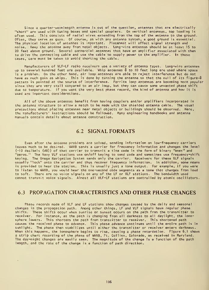
Since a quarter-wavelength antenna is out of the question, antennas that are electrically"short" are used with tuning boxes and special couplers. On vertical antennas, top loading is
often used. This consists of radial wires extending from the top of the antenna to the ground.
Often, they serve as guys. Of course, as with any antenna system, a good ground is essential.The physical location of antennas is important. Placement will affect signal strength and
noise. Keep the antenna away from metal objects. Long-wire antennas should be at least 15 to
20 feet above ground. Several commercial antennas that have an amplifier associated with them
to drive the connecting cable and use the cable to supply power to the amplifier. In those
cases, care must be taken to avoid shorting the cable.
Manufacturers of VLF-LF radio receivers use a variety of antenna types. Long-wire antennas
up to several hundred feet are available. Whip antennas 8 to 10 feet long are used where space
is a problem. On the other hand, air loop antennas are able to reject interference but do not
have as much gain as whips. This is done by turning the antenna so that the null of its figure-8
pattern is pointed at the source of interference. Ferrite loop antennas are becoming more popular
since they are very small compared to an air loop, but they can cause some unwanted phase shift
due to temperature. If you want the very best phase record, the kind of antenna and how it is
used are important considerations.
All of the above antennas benefit from having couplers and/or amplifiers incorporated in
the antenna structure to allow a match to be made with the shielded antenna cable. The usual
precautions about placing antennas near metal objects or buildings should be observed. Here,
the manufacturers' instructions should be followed. Many engineering handbooks and antennamanuals contain details about antenna construction.
6.2 SIGNAL FORMATS
Even after the antenna problems are solved, sending information on low-frequency carriersleaves much to be desired. WWVB sends a carrier for frequency information and changes the level
(-10 decibels (dB) ) of that carrier to transmit a time code in the form of binary "ones" and
"zeros." The Navy VLF stations use on/off keying to send code and sometimes use frequency-shiftkeying. The Omega Navigation System sends only the carrier. Receivers for these VLF signalsusually "lock" onto the carrier and thus recover frequency information. In addition, some meansis provided to hear the station. This is usually just a tone output. For example, if you wereto listen to WWVB, you would hear the one-second code segments as a tone that changes from loud
to soft. There are no voice signals on any of the LF or VLF stations. The bandwidth used
cannot transmit voice signals. Almost all VLF-LF stations are controlled by atomic oscillators.
6.3 PROPAGATION CHARACTERISTICS AND OTHER PHASE CHANGES
Phase records made of VLF and LF stations show changes caused by the daily and seasonal
changes in the propagation path. Among other things, LF and VLF signals have regular phaseshifts. These shifts occur when sunrise or sunset occurs on the path from the transmitter to
receiver. For instance, as the path is changing from all darkness to all daylight, the iono-sphere lowers. This shortens the path from transmitter to receiver. This shortened pathcauses the received phase to advance. This phase advance continues until the entire path is in
sunlight. The phase then stabilizes until either the transmitter or receiver enters darkness.When this happens, the ionosphere begins to rise, causing a phase retardation. Figure 6.1 showsa strip chart recording of the phase of WWVB, Ft. Collins, Colorado, as received in Maryland.The day-night changes are easily seen. The magnitude of the change is a function of the pathlength, and the rate of the change is a function of path direction.
106
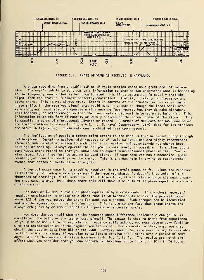
p SUNSET GREENBELT MO
r SUNSET BOULDER. COLO
.1,
SUNRISE 6REENBELT. MO
>- SUNRISE BOULDEF . COLO
SUNSET BOULDEF
SUNSET6REENBELT. MO.
. COLO - SUNRISE BOULDER. COLO -,
SUNRISE GREENBELT. MO -
EtJ- 41 -I ......III— ii|
Hjl 1!i WWVB IN TERMS OF WWV
CONTROLLING OSCILLATOR'JUNE 3.4 & 5.
'l II II
i -
r1 41 ~I
1
I
1
! J iffllhl IIIN ~i
j 411 + *1
':.!]1 1
SLOPE +1 M««/2w -it—— in;j
ji
: i : !
• HRS (1800-1800 UT) " "*
Hi-:IJLIi
)0 usic U-H-'J
1-j- 4-J4-i-!- i
— 4-+-^- 1 WWVB IS MO " pis ABOVE WWV. 1 z- -7=-
M1MIi[i:::±: i* j
j
-j-j--(-i-I-]
' illutrf w i:±::::i!! >"i-J^-.z-A-.2-.i
: = ( III—~* 't i
\ II! i
i 1; i i MM ?4HiiT t___
liisi^!ii::::E1
+ -+ -i + 4-J—1
1
j1
ifH- -h4+- .»>**-<| ±y±e
;
'! 'in4444--.4^-£:::EEi::Ei::i—-L-PWSK««
TIME(UTC)
FIGURE 6.1. PHASE OF WWVB AS RECEIVED IN MARYLAND.
A phase recording from a stable VLF or LF radio station contains a great deal of informa-tion. The user's job is to sort out this information so that he can understand what is happeningto the frequency source that is being calibrated. His first assumption is usually that thesignal from the station is almost perfectly controlled. That is, it starts on frequency andstays there. This is not always true. Errors in control at the transmitter can cause largephase shifts in the received signal that would make it appear as though the local oscillatorwere changing. Most stations operate with a near perfect record, but they do make mistakes.This happens just often enough so that the user needs additional information to help him. Thisinformation takes the form of monthly or weekly notices of the actual phase of the signal. Thisis usually in terms of microseconds advance or retard. A sample of NBS data for WWVB and othermonitored stations is shown in figure 6.2. U. S. Naval Observatory (USNO) data for its stationsare shown in figure 6.3. These data can be obtained free upon request.
The implication of possible transmitting errors to the user is that he cannot hurry throughcalibrations! Certain practices with respect to LF radio calibrations are highly recommended.These include careful attention to such details as receiver adjustments—do not change knobsettings or cabling. Always operate the equipment continuously if possible. This gives you acontinuous chart record so that you know when to expect sunrise/sunset phase shifts. You canalso detect local interference and noise conditions. If your receiver has a mechanical phasecounter, jot down the readings on the chart. This is a great help in trying to reconstructevents that happen on weekends or at night.
A typical occurrence for a tracking receiver is the cycle phase shift. Since the receiveris faithfully following a zero crossing of the received phase, it doesn't know which of thethousands of crossings it is locked to. If it loses lock, it will simply go to the next cross-ing that comes along. On a phase chart this will show up as a shift in phase equal to one cycleof the carrier.
For WWVB at 60 kHz, a cycle of phase equals 16.67 microseconds. If the chart recorder/receiver combination is producing a chart that is 50 microseconds across, the pen will moveabout 1/3 of the way across the chart for each cycle change. Such changes can be identifiedand must be ignored during calibration runs. This is due to the fact that phase charts arealways ambiguous by an amount equal to the period of a carrier cycle.
How does the user tell whether the recorded phase difference indicates a change in hisoscillator, the path, or the transmitted signal? The answer is that he knows from experience!If you plan to use VLF or LF signals for frequency calibrations, you must become very familiarwith the characteristics of the signals you are using. For accurate calibrations, you mustobtain the station data from NBS or the USNO. Battery backup for receivers is highly desirable--in fact, almost necessary if you plan to calibrate precise oscillators over a period of manydays. All of this may sound like a hopeless task, but it isn't. The results are worth theeffort when you consider that you can perform calibrations up to 1 part in lO^ 1 in 2k hours.
107
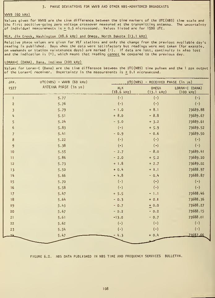
3. PHASE DEVIATIONS FOR WWVB AND OTHER NBS -MONITORED BROADCASTS
WWVB (60 kHz)
r WWVB are the time difference betwee n the time mar kers of the UTC(NBS) timeValues g iven fc scale andthe first positive-going zero voltage crossover measured at tr e transmitting antenna. The uncertaintyof indiv 'dual measurements is + 0.5 microsecond. Va 1 ues 1 i sted are fo - 1500 UTC.
NLK, Jim Creek, Washington (18.6 kHz) anc Omega, Nor th Dakota (13. 1 kH
ava iRelative phase values are given for VLF stations and only the change f "om the previous able day'sread ing 's publ ished. Day s when the date were satis factory but readings were not taken (foi• example,on weekeiids or station maintenance days) are mar <ed (-) . If data are ost, continuity is a so lost
and the 'ndication is ("), which means that read ing cannot be compa red to the previous day.
LORAN-C (DANA)
,
Dana, Indiana (100 kHz)
fference between the UTC( NBS) time pulses and theValues for Loran-C (Dana) are the time d" pps outputof the Loran-C receiver. Uncertainty in the measurements is H
:°- 1 microsecond
.
JAN.
1977
UTC(NBS) - WWVB (60 kHz)
ANTENNA PHASE (in us)
UTC( NBS) - RECEIVED PHASE (in us)
NLK OMEGA 1.0RAN--C (DANA)
(18.6 kh z) (13.1 kHz) (100 kHz)
1 5.77 (-) (") (-)
2 5.76 (-) (-) (-)
3 5.79 - 1 .0 + 8.1 73689.88
4 5.51 + 8.0 - 8.8 73689.67
5 5.2/* - 5.0 + 3.2 73689.61
6 5.83 (-) + 5.9 73689.52
7 5.41 - 0.9 - 0.6 73689.50
8 5.22 (-) (-) (-)
9 5.38 (-) (-) (-)
10 5-55 - 2.7 - 8.0 73689.41
11 5.86 - 2.0 + 5.2 73689.20
12 5.73 + 1.8 + 2.7 73689.02
13 5.50 + 0.4 + 1 .1 73688.97
14 5.66 - 4.8 - 0.4 73688.87
15 5.70 (-) (-) (-)
16 5.58 (-) (-) (-)
17 5.^7 + 5.5 -1.1 73688.46
18 5.64 - 0.3 + 0.1 73688.36
19 5.^3 - 0.7 + 0.0 73688.27
20 5.67 - 0.2 - 0.2 73688. T5
21 5.61 -13-0 - 0.7 73688.01
22 5.62 (-) (-) (-)
23 5-54
5.47
(-)
-^-4.3
(")
+ 0.4
(-)
7^687.66J • > / ^
FIGURE 6.2. NBS DATA PUBLISHED IN NBS TIME AND FREQUENCY SERVICES BULLETIN.
108
U. S. NAVAL OBSERVATORYWASHINGTON, D.C. 20390
DAILY PHASE VALUES AND TIME DIFFERENCES SERIES 4
THE TABLE GIVES: UTC(USNO MC) - TRANSMITTING STATION
20 JANUARY 1977
NO. 520
UNIT = ONE MICROSECOND
LC/9970 LC/4990 LC/9930 LC/7970 LC/7990 LC/7930 LC/5930 LC/9940FREQUENCY NW PAC. CEN. PAC. E. COAST NOR. SEA MED. SEA N. ATL. N. PAC. W. COASTkHz (UTC)
MJD100 100 100 100 100 100 100 100
JAN. 10 43153 -0.8 (4) -0.1 (5) 1.64 -2.1 -3.5 0.4 -3.6 2.5 (9
11 43154 -0.8 0.0 1.31 -2.4 -3.9 0.3 -3.5 2.612 43155 -0.8 0.1 1.28 -2.6 -4.1 0.2 -3.4 2.8
13 43156 -0.7 0.2 1.13 -2.7 -4.1 0.2 -3.4 3.014 43157 -0.6 0.4 1.17 -2.5 -3.9 0.3 -3.2 3.1
15 43158 -0.4 0.4 1.21 -2.2 -3-7 0.5 - 3.316 43159 -0.4 0.3 1.03 -2.4 -3.9 0.5 - 3.517 43160 -0.3 0.4 0.60 -3.2 -4.7 0.1 - 3.618 43161 -0.3 0.4 0.60 -2.9 - 0.1 - 3.7
19 43162 -0.3 0.6 0.58 - - 0.2 - 3.9
3 6 7 1 1 2 5
LD/4930 O/ND O/ND 0/L 0/T 0/H GBR NLK NBAFREQUENCY W. COAST 13.1 13.6 13.6 13.6 RADIATED 16.0 18.6 24.0kHz (UTC)
MJD100 6MS+ 6MS+ 25MS+ 11MS+ 19MS+ 12MS+ 11MS+
JAN. 13 43156 -50.7 417 419 149 621 - 519 480 -
14 43157 -50.9 417 419 149 622 - 517 475 -
15 43158 - 418 419 150 622 - 517 476 -
16 43159 - 417 418 150 622 - 516 476 -
17 43160 -51.4 417 418 149 621 - 514 481 -
18 43161 -51.7 417 418 147 620 - 515 481 -
19 43162 -51.6 417 418 148 621 518 480
REFERENCES: (A) TIME SERVICE INFORMATION LETTER OF 15 AUGUST 1973(B) TIME SERVICE ANNOUNCEMENT, SERIES 9, NO. 105 (LORAN-C)
(c) DAILY PHASE VALUES AND TIME DIFFERENCES, SERIES 4, NO. 389 (LORAN-D)
NOTES: (1) PROPAGATION DISTURBANCES WERE OBSERVED NEAR THE FOLLOWING TIMES:
19 JAN. 1520/3, 1655/2.
(2) NAVY STATIONS OFF-AIR TIMES:
NWC 12 JAN. 0802 TO 0851 UT, 1225 TO 1238 UT
13 JAN. 0008 TO 0200 UT
14 JAN. 1640 TO 1644 UT
19 JAN. 0941 TO 1001 UT
SCHEDULED TO EXTEND MAINTENANCE PERIOD TO 0600 UT ON 26 JAN.,
9 FEB., 23 FEB., AND 9 MAR.
NLK 12 JAN. 2345 TO 2353 UT
13 JAN. 0037 TO 0047 UT, 0135 TO 0152 UT
(3) OMEGA STATIONS OFF-AIR TIMES (FROM COAST GUARD ONSOD, WASHINGTON, D.C):
HAWAII 6 JAN. 1831 TO 1832 UT, 2210 TO 2212 UT
11 JAN. 2302 TO 2303 UT
12 JAN. 0718 TO 0719 UT, 9822 TO 0823 UT
13 JAN. 2045 TO 2046 UT
FIGURE 6.3. USNO PHASE DATA, PUBLISHED WEEKLY.
109
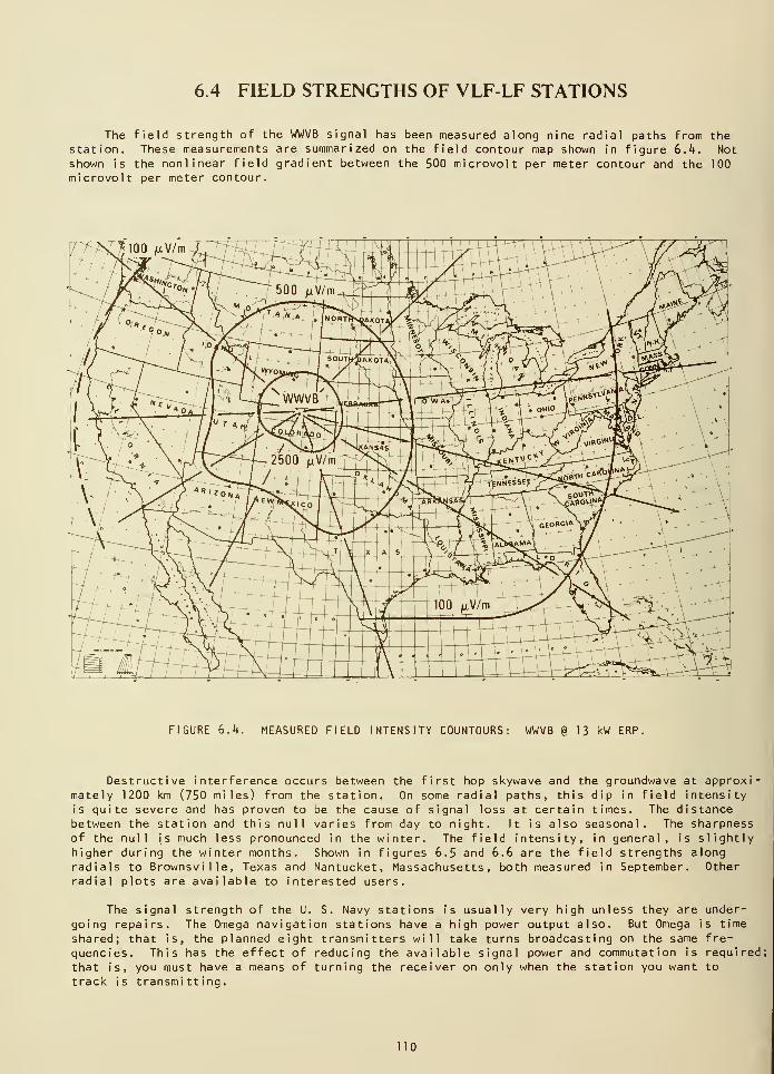
6.4 FIELD STRENGTHS OF VLF-LF STATIONS
The field strength of the WWVB signal has been measured along nine radial paths from thestation. These measurements are summarized on the field contour map shown in figure 6.4. Not
shown is the nonlinear field gradient between the 500 microvolt per meter contour and the 100
microvolt per meter contour.
FIGURE 6.4. MEASURED FIELD INTENSITY C0UNT0URS: WWVB g 13 kW ERP.
Destructive interference occurs between the first hop skywave and the groundwave at approxi-mately 1200 km (750 miles) from the station. On some radial paths, this dip in field intensityis quite severe and has proven to be the cause of signal loss at certain times. The distancebetween the station and this null varies from day to night. It is also seasonal. The sharpnessof the null is much less pronounced in the winter. The field intensity, in general, is slightlyhigher during the winter months. Shown in figures 6.5 and 6.6 are the field strengths alongradials to Brownsville, Texas and Nantucket, Massachusetts, both measured in September. Otherradial plots are available to interested users.
The signal strength of the U. S. Navy stations is usually very high unless they are under-
going repairs. The Omega navigation stations have a high power output also. But Omega is time
shared; that is, the planned eight transmitters will take turns broadcasting on the same fre-
quencies. This has the effect of reducing the available signal power and commutation is required:
that is, you must have a means of turning the receiver on only when the station you want to
track is transmitting.
110
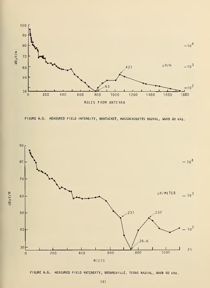
3.
-10
-10'
-10'
600 800 1000 1200
MILES FROM ANTENNA
1400 1600 1800
FIGURE 6.5. MEASURED FIELD INTENSITY, NANTUCKET, MASSACHUSETTS RADIAL, WWVB 60 kHz.
90 r
PLCO-o
yV/METER _ 1Q3
-10
10'
25
MILES
FIGURE 6.6. MEASURED FIELD INTENSITY, BROWNSVILLE, TEXAS RADIAL, WWVB 60 kHz.
Ill
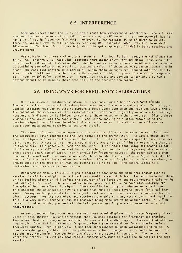
6.5 INTERFERENCE
Some WWVB users along the U. S. Atlantic coast have experienced interference from a Britishstandard frequency radio station, MSF. Some years ago, MSF was not only lower powered, but it
was also offset in frequency from WWVB. However, it now radiates 25 kW of power on 60 kHz.There are various ways to tell if one is receiving MSF instead of WWVB. The 45° phase shift(discussed in Section 6.6.1, figure 6.9) should be quite apparent if WWVB is being received andphase-tracked.
One solution is to use a directional antenna. If a loop is being used, the MSF signal canbe nulled. Eastern U. S. receiving locations from Boston south that are using loops should be
able to null MSF and still receive WWVB. Another method is to produce a unidirectional antennaby combining the voltages induced in a loop and a whip. If these two voltages are equal and in
phase, the resultant pattern is a cardioid. Since these voltages are induced into the whip by
theelectric field, and into the loop by the magnetic field, the phase of the whip voltage mustbe shifted by 90° before combination. Interested readers are advised to consult a suitableantenna manual or to discuss their problems with the receiver manufacturer.
6.6 USING WWVB FOR FREQUENCY CALIBRATIONS
Our discussion of calibrations using low-frequency signals begins with WWVB (60 kHz).
Frequency calibrations usually involve phase recordings of the received signals. Typically, a
special tracking receiver is used to compare a local oscillator with the received WWVB signals.
The output of the receiver can be displayed on its front panel digitally or as a meter reading.However, this discussion is limited to making a phase record on a chart recorder. Often, theserecorders are built into the receivers. Since we are looking at a phase recording of the
received signal, we will see the effect of any path changes. In addition, we will see our
oscillator phase change relative to the WWVB signal.
The amount of phase change depends on the relative difference between our oscillator and
the cesium oscillator controlling the WWVB signal at the transmitter. The sample phase chart
shown in figure 6.7 has very little oscillator drift. This is because a quality oscillator wasbeing measured. A more typical record would have a whole series of lines crossing the chart as
in figure 6.8. This poses a dilemma for the user. If the oscillator being calibrated is far
off frequency from WWVB, he needs either a fast chart or one that displays many microseconds ofphase across the width of paper. For high-quality frequency sources, the paper can be slowed
down or the chart width, in microseconds, can be reduced. The user is encouraged to study the
manuals for the particular receiver he is using. If the user is planning to buy a receiver, he
should consider the problem of what the record is going to look like before selecting a
particular receiver/recorder combination.
Measurements made with VLF-LF signals should be done when the path from transmitter to
receiver is all in sunlight. An all dark path would be second choice. The sunrise/sunset phase
shifts (called diurnals) will affect the accuracy of calibrations and measurements should not be
made during these times. There are other sudden phase shifts due to particles entering the
ionosphere that can affect the signal. These usually last only ten minutes or a half-hour.
This explains the advantage of having a chart that runs at least several hours for a calibra-
tion. During sudden phase shifts, the signal level may drop. Most receivers have a meter for
signal strength, but the more elaborate receivers are able to chart record the signal amplitude.This is a very useful record if the calibrations being made are to be within parts in 10 IU or
better. In other words, you need all the help you can get if you are to make the very best
measurements.
As mentioned earlier, some receivers use front panel displays to indicate frequency offset.
Later in this chapter, we mention methods that use oscilloscopes for frequency calibration.Even a zero-beat or Lissajous method could be used with the WWVB signal. Remember that what you
are getting from WWVB is a standard frequency signal that started out from a nearly perfect
frequency source. When it arrives, it has been contaminated by path variations and noise. A
chart recorder giving a history of the path and oscillator changes is very handy to have. To
get the best resolution from the WWVB signals, a chart record is mandatory. The results are
worth the effort. As with any measurement, extreme care must be exercised to realize the best
resul ts.
112
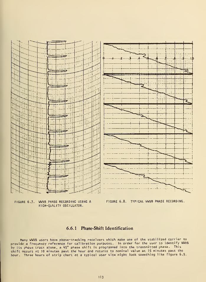
FIGURE 6.7. WWVB PHASE RECORDING US
HIGH-QUALITY OSCILLATORFIGURE 6.8. TYPICAL WWVB PHASE RECORDING,
6.6.1 Phase-Shift Identification
Many WWVB users have phase-tracking receivers which make use of the stabilized carrier to
provide a frequency reference for calibration purposes. In order for the user to identify WWVB
by its phase track alone, a ^5° phase shift is programmed into the transmitted phase. This
shift occurs at 10 minutes past the hour and returns to nominal value at 15 minutes past the
hour. Three hours of strip chart at a typical user site might look something like figure 6.9.
13
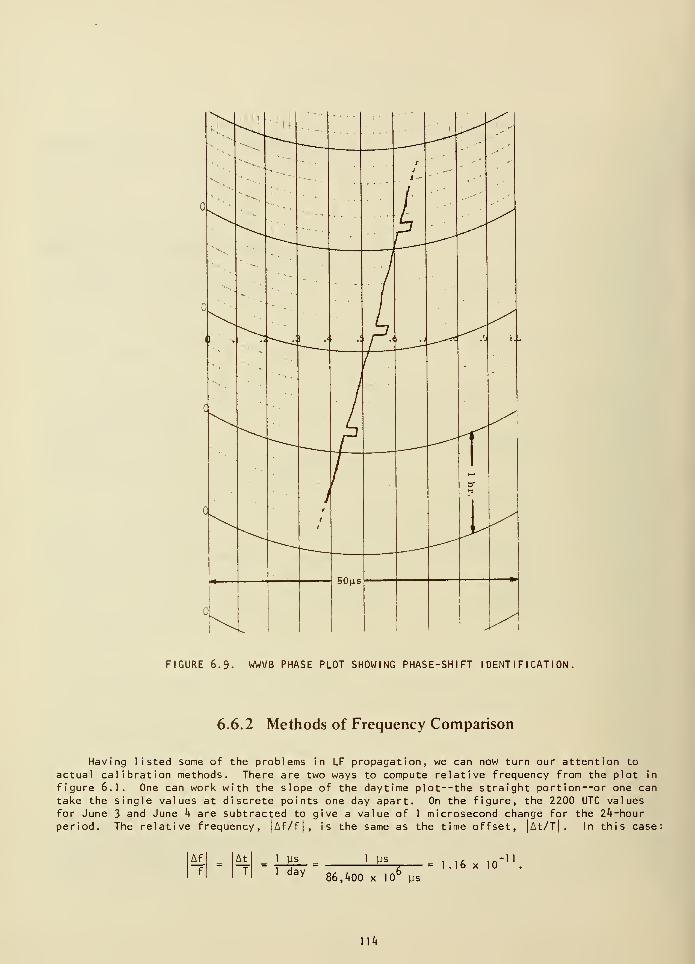
FIGURE 6.9- WWVB PHASE PLOT SHOWING PHASE-SHIFT IDENTIFICATION,
6.6.2 Methods of Frequency Comparison
Having listed some of the problems in LF propagation, we can now turn our attention to
actual calibration methods. There are two ways to compute relative frequency from the plot in
figure 6.1. One can work with the slope of the daytime plot--the straight portion--or one can
take the single values at discrete points one day apart. On the figure, the 2200 UTC values
for June 3 and June k are subtracted to give a value of 1 microsecond change for the 2^-hourperiod. The relative frequency, |Af/f|, is the same as the time offset, At/T[ . In this case:
1 ys
1 day1 ys
= 1.1686,/»00 x 10 us
10•1
]\k
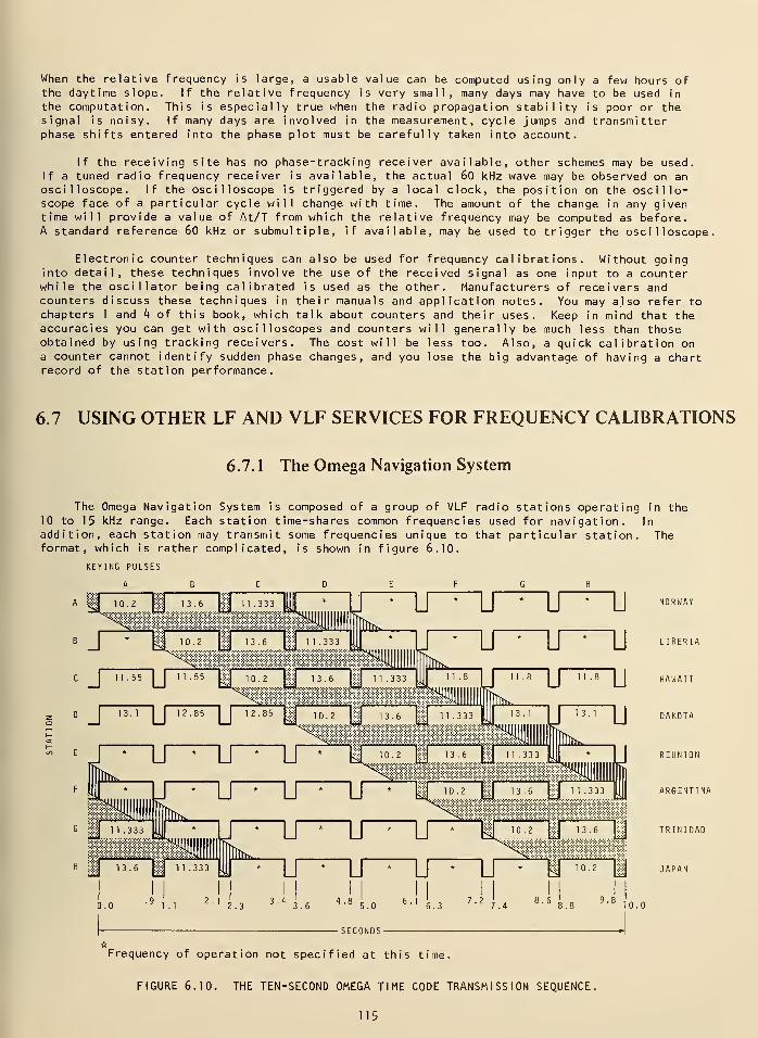
When the relative frequency is large, a usable value can be computed using only a few hours ofthe daytime slope. If the relative frequency is very small, many days may have to be used in
the computation. This is especially true when the radio propagation stability is poor or thesignal is noisy. If many days are involved in the measurement, cycle jumps and transmitterphase shifts entered into the phase plot must be carefully taken into account.
If the receiving site has no phase-tracking receiver available, other schemes may be used.If a tuned radio frequency receiver is available, the actual 60 kHz wave may be observed on anoscilloscope. If the oscilloscope is triggered by a local clock, the position on the oscillo-scope face of a particular cycle will change with time. The amount of the change in any giventime will provide a value of At/T from which the relative frequency may be computed as before.A standard reference 60 kHz or submultiple, if available, may be used to trigger the oscilloscope,
Electronic counter techniques can also be used for frequency calibrations. Without goinginto detail, these techniques involve the use of the received signal as one input to a counterwhile the oscillator being calibrated is used as the other. Manufacturers of receivers andcounters discuss these techniques in their manuals and application notes. You may also refer to
chapters 1 and k of this book, which talk about counters and their uses. Keep in mind that theaccuracies you can get with oscilloscopes and counters will generally be much less than thoseobtained by using tracking receivers. The cost will be less too. Also, a quick calibration ona counter cannot identify sudden phase changes, and you lose the big advantage of having a chartrecord of the station performance.
6.7 USING OTHER LF AND VLF SERVICES FOR FREQUENCY CALIBRATIONS
6.7. 1 The Omega Navigation System
The Omega Navigation System is composed of a group of VLF radio stations operating in the10 to 15 kHz range. Each station time-shares common frequencies used for navigation. In
addition, each station may transmit some frequencies unique to that particular station. Theformat, which is rather complicated, is shown in figure 6.10.
KEYING PULSES
w E
lT^j^^j^^J
Frequency of operation not specified at this time.
FIGURE 6.10. THE TEN-SECOND OMEGA TIME CODE TRANSMISSION SEQUENCE.
115
10.0
NORWAY
LIBERIA
HAWAII
DAKOTA
REUNION
ARGENTINA
TRINIDAD
JAPAN
If one wishes to use an Omega station for frequency calibration, a phase-tracking receiveris highly recommended. If one of the navigation frequencies is to be used, then an Omegacommutator must also be used. This is a device that turns the phase-tracking receiver on andoff at the proper times to receive only the desired Omega station.
The frequencies and the format segments of the Omega stations are derived from cesium beamoscillators. The USNO monitors and reports the Omega stations' phase values. These stationsradiate a nominal 10 kW of power. This power level should be sufficient to allow the user to
receive at least three stations no matter where he is located.
6.7.2 NLK, NAA, and MSF
Currently, several U. S. Naval Communications stations provide signals that can be used to
steer frequency standards. In the northeastern U. S., NAA (Cutler, Maine) at 17.8 kHz can be
used if WWVB cannot be received. NLK on 18.6 kHz broadcasts from Washington State. A word ofcaution concerning MSF, NAA, or any other communications station: Use of these stations for
frequency calibration is strictly secondary to their primary function which is military com-munications. These stations are subject to frequency changes, outages, and changes in schedule.The only radio station in the LF or VLF range in the U. S. that is strictly for time andfrequency use is WWVB.
6.8 MONITORING DATA AVAILABILITY
No matter which station is chosen as a basis for ca 1 i bration--WWVB, Omega, or VLF--the usermust be on a mailing list to receive notices of changes in operation schedule. WWVB currentlyoperates 24-hours a day every day. No changes in operating format are made without advancenotification. The Omega stations do schedule maintenance outages and some low-power operations.As the system becomes fully operational, these should diminish. Announcements regarding the
status of the various Omega stations in the Omega Navigation System are given hourly on bothWWV and WWVH. See figure 11.1 in Chapter 11 for announcement times. The Navy VLF stations are
the ones most likely to change their mode of operation without notification.
Currently, NBS and USNO are monitoring and reporting the phase differences of NLK, Omega,
and the East Coast Loran-C stations. In addition, NBS monitors and reports phase differencesfor WWVB and the USNO offers data on NAA. These data are available to interested users by
contacting the Time and Frequency Division of NBS or the USNO.
6.9 USING THE WWVB TIME CODE
WWVB transmits a special binary-coded-decimal time code that provides time information.This service is used by seismologists, standards labs, commercial power companies, and othersinterested in synchronizations with accuracies of the order of 0.1 to 50 milliseconds. The code
provides information of days, hours, and minutes. Seconds are resolved by counting bits. A
correction, applied to the transmitted time to obtain earth time, UT1 , is also provided for use
by some astronomers and navigators.
Unlike a code that is designed primarily for machine decoding, the WWVB code was originallydesigned to be manually decoded from strip chart recordings or tapes. To simplify this processfor a human decoder, the bits are placed such that the most significant bit occurs first in each
code word. The actual bit itself, whether a binary zero, binary one, or position identifier, is
determined by the duration of the power reduction of the transmitted carrier.
116
6.9. 1 Time Code Format
The WWVB time code is generated by shifting the power of the 60-kHz carrier. The carrierpower is reduced 10 dB at the beginning of each second and restored to full power 200 millisecondslater for a binary zero, 500 milliseconds later for a binary one, and 800 milliseconds later for
a reference marker or position identifier. Certain groups of pulses are encoded to representdecimal numbers which identify the minute, hour, and day of year. The binary-to-decimal weight-ing scheme is 8-4-2-1 with the most significant binary digit transmitted first. Note that thisweighting sequence is the reverse of the WWV/WWVH code. The BCD groups and their basic decimalequivalents are tabulated below:
BINARY GROUP DECIMALWEIGHT: 8 4 2 1 EQUIVALENT
1
1
1 1
1
1 1
1 1
1 1 1
1
1 1
1
2
3
4
5
6
7
8
9
The decimal equivalent of each group is derived by multiplying the individual binary digitsby the weight factor of their respective columns and then adding the four products together.For example, the binary sequence 1001 in 8-4-2-1 code is equivalent to (1 x 8) + (0 x 4) + (0 x 2)
+ (1 x 1 ) = 8 + + + 1 = 9, as shown in the table. If fewer than nine decimal digits arerequired, one or more of the high-order binary digits may be dispensed with.
Once every minute, in serial fashion, the code format presents BCD numbers corresponding to
the current minute, hour, and day on the UTC scale. Two BCD groups identify the minute (00
through 59); two groups identify the hour (00 through 23); and three groups identify the day ofyear (001 through 366). When representing units, tens, or hundreds, the basic 8-4-2-1 weightsare multiplied by 1, 10, or 100 respectively. The coded information refers to the time at thebeginning of the one-minute frame. Within each frame, the seconds may be determined by countingpul ses
.
Every new minute commences with a frame reference pulse which lasts for 0.8 second. Also,every ten-second interval within the minute is marked by a position identifier pulse of 0.8-
second duration.
UT1 corrections to the nearest 0.1 second are transmitted at seconds 36 through 44 of eachframe. Coded pulses at 36, 37, and 38 seconds indicate the positive or negative relationship of
UT1 with respect to UTC. Pulses at 36 and 38 seconds are transmitted as binary ones only if UT1
is early with respect to UTC, in which case a correction must be added to the UTC signals to
obtain UT1 . The pulse transmitted at 37 seconds is a binary one if UT1 is late with respect to
UTC, in which case the required UT1 correction must then be subtracted. The magnitude of the
UT1 correction is transmitted as a BCD group at 40, 41, 42, and 43 seconds. Because UT1 cor-rections are expressed in tenths of seconds, the basic 8-4-2-1 weight of that particular binarygroup is multiplied by 0.1 to obtain its proper decimal equivalent.
Figure 6.11 shows a sample frame of the time code in rectified or dc form. The negative-going edge of each pulse coincides with the beginning of a second. Position identifiers arelabeled P] , P2, P3, P/j, P5, and Pq. Brackets show the demarcation of the minutes, hours, days,and UT1 sets. The applicable weight factor is printed beneath the coded pulses in each BCD
group. Except for the position identifiers and the frame reference marker, all uncoded pulsesare binary zeros.
17
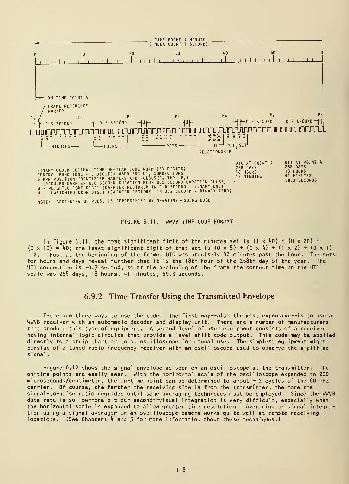
rTIME FRAME 1 MINUTE
( INDEX COUNT 1 SECOND)
I I I I I ' ' ' 'I I I '
10 20 30 40 50
i I I I I I I I I l I I I I I I I I I I 1 I I I I I 1 I I I I I I I I I 1I I I I I I I I I
ON TIME POINT A
•FRAME REFERENCEMARKER
Pi P„ P 5 Po
hV 0.3 SECOND —-{I
— . 2 SECOND —|W|
—
-jU|- —j
|—0.5 SECOND .8 SECOND -| (j"
-i n nnnnirinjTLfirnr^^
IQ => Q d ° o o
L UTrJ LUT, SET J
MINUTES- HOURS DAYS
RELATIONSHIP
UTC AT POINT A UT1 AT POINT A
BINARY COOED DECIMAL TIME-OF-YEAR CODE WORD (23 DIGITS)?fl
8H nnRS l^HOURS
CONTROL FUNCTIONS (15 DIGITS) USED FOR UT , CORRECTIONS 18 HOURS 18 HOURS
6 PPM POSITION IDENTIFIER MARKERS AND PULSES (P„ THRU P 5 )42 MINUTES
50 3 SECONDS(REDUCED CARRIER 0.8 SECOND DURATION PLUS 0.2 SECOND DURATION PULSE) •
59.3 SECONDS
W - WEIGHTED CODE DIGIT (CARRIER RESTORED IN 0.5 SECOND - BINARY ONE)
U - UNWEIGHTED CODE DIGIT (CARRIER RESTORED IN 0.2 SECOND - BINARY ZERO)
NOTE: BEGINNING OF PULSE IS REPRESENTED BY NEGAT I VE - GOING EDGE.
FIGURE 6.11. WWVB TIME CODE FORMAT.
In figure 6.11, the most significant digit of the minutes set is (1 x kO) + (0 x 20) +
(0 x 10) = kO; the least significant digit of that set is (0 x 8) + (0 x ^) + (1 x 2) + (0 x 1)
= 2. Thus, at the beginning of the frame, UTC was precisely hi minutes past the hour. The sets
for hours and days reveal further that it is the 1 8th hour of the 258th day of the year. The
UT1 correction is -0.7 second, so at the beginning of the frame the correct time on the UT1
scale was 258 days, 18 hours, *4l minutes, 59 - 3 seconds.
6.9.2 Time Transfer Using the Transmitted Envelope
There are three ways to use the code. The first way
—
also the most expensive— is to use a
WWVB receiver with an automatic decoder and display unit. There are a number of manufacturersthat produce this type of equipment. A second level of user equipment consists of a receiverhaving internal logic circuits that provide a level shift code output. This code may be applieddirectly to a strip chart or to an oscilloscope for manual use. The simplest equipment mightconsist of a tuned radio frequency receiver with an oscilloscope used to observe the amplifieds ignal
.
Figure 6.12 shows the signal envelope as seen on an oscilloscope at the transmitter. Theon-time points are easily seen. With the horizontal scale of the oscilloscope expanded to 200microseconds/centimeter, the on-time point can be determined to about +2 cycles of the 60 kHzcarrier. Of course, the farther the receiving site is from the transmitter, the more thesignal-to-noise ratio degrades until some averaging techniques must be employed. Since the WWVBdata rate is so low--one bit per second—visual integration is very difficult, especially whenthe horizontal scale is expanded to allow greater time resolution. Averaging or signal integra-tion using a signal averager or an oscilloscope camera works quite well at remote receivinglocations. (See Chapters k and 5 for more information about these techniques.)
118
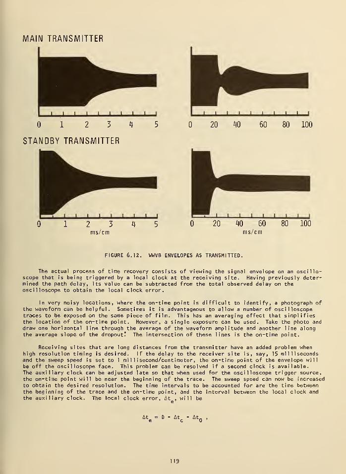
MAIN TRANSMITTER
12 3 4
STANDBY TRANSMITTER
20 40 60 80 100
ms/cm ms/cm
FIGURE 6.12. WWVB ENVELOPES AS TRANSMITTED.
The actual process of time recovery consists of viewing the signal envelope on an oscillo-scope that is being triggered by a local clock at the receiving site. Having previously deter-mined the path delay, its value can be subtracted from the total observed delay on theoscilloscope to obtain the local clock error.
In very noisy locations, where the on-time point is difficult to identify, a photograph ofthe waveform can be helpful. Sometimes it is advantageous to allow a number of oscilloscopetraces to be exposed on the same piece of film. This has an averaging effect that simplifiesthe location of the on-time point. However, a single exposure can be used. Take the photo and
draw one horizontal line through the average of the waveform amplitude and another line alongthe average slope of the dropout! The intersection of these lines is the on-time point.
Receiving sites that are long distances from the transmitter have an added problem whenhigh resolution timing is desired. If the delay to the receiver site is, say, 15 millisecondsand the sweep speed is set to 1 millisecond/centimeter, the on-time point of the envelope will
be off the oscilloscope face. This problem can be resolved if a second clock is available.The auxiliary clock can be adjusted late so that when used for the oscilloscope trigger source,the on-time point will be near the beginning of the trace. The sweep speed can now be increasedto obtain the desired resolution. The time intervals to be accounted for are the time betweenthe beginning of the trace and the on-time point, and the interval between the local clock andthe auxiliary clock. The local clock error, At , wi 1 1 be
At D - At At,
119
where: D is the propagation delay,
At is the interval between the two clocks,c
Atn
is the trace delay on the oscilloscope.
If Ate is positive, then the local clock pulse occurs after the transmitted time pulse.
If At is negative, the local clock pulse occurs first.
6.10 SUMMARY
Although you can get better accuracies by using LF and VLF broadcasts than you can fromHF broadcasts, use of these signals poses special problems that are not encountered at HF.
But if you need frequency accuracies of a part in 10'' or better, or time synchronizationfrom 50 milliseconds to 100 microseconds, VLF or LF broadcasts may suit your needs very well.
However, you must be willing the spend the time, money, and effort necessary to get maximumresul ts
.
You do have an alternative, though. The frequency calibration service using networktelevision and the TV Line-10 method of obtaining time and/or frequency may be less expensiveand easier to use.
120
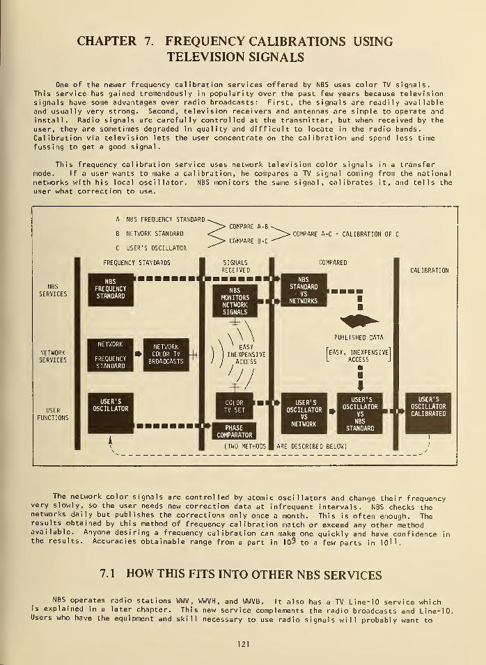
CHAPTER 7. FREQUENCY CALIBRATIONS USINGTELEVISION SIGNALS
One of the newer frequency calibration services offered by NBS uses color TV signals.This service has gained tremendously in popularity over the past few years because televisionsignals have some advantages over radio broadcasts: First, the signals are readily availableand usually very strong. Second, television receivers and antennas are simple to operate and
install. Radio signals are carefully controlled at the transmitter, but when received by the
user, they are sometimes degraded in quality and difficult to locate in the radio bands.
Calibration via television lets the user concentrate on the calibration and spend less timefussing to get a good signal.
This frequency calibration service uses network television color signals in a transfermode. If a user wants to make a calibration, he compares a TV signal coming from the nationalnetworks with his local oscillator. NBS monitors the same signal, calibrates it, and tells theuser what correction to use.
NBS
SERVICES
NETWORKSERVICES
USER
FUNCTIONS
A NBS FREQUENCY STANDARD
B NETWORK STANDARD
C USER'S OSCILLATOR
FREQUENCY STANDARDS
COMPARE A-C = CALIBRATION OF C
NBSFREQUENCYSTANDARD
FREQUENCYSTANDARD
USER'SOSCILLATOR
NETWORKCOLOR TV
BROADCASTS
SIGNALS
RECEIVED
NBSMONITORSNETWORKSIGNALS
t 1
PHASECOMPARATOR
(TWO METHODS
COMPARED
NBSSTANDARD
VSNETWORKS
USER'SOSCILLATOR
VS
NETWORK
PUBLISHED DATA
EASY, INEXPENSIVEACCESS
USER'SOSCILLATOR
VS
NBSSTANDARD
ARE DESCRIBED BELOW)
CALIBRATION
MUSER'S
OSCILLATORCALIBRATED
The network color signals are controlled by atomic oscillators and change their frequencyvery slowly, so the user needs new correction data at infrequent intervals. NBS checks thenetworks daily but publishes the corrections only once a month. This is often enough. Theresults obtained by this method of frequency calibration match or exceed any other methodavailable. Anyone desiring a frequency calibration can make one quickly and have confidence inthe results. Accuracies obtainable range from a part in 1C>9 to a few parts in 10".
7. 1 HOW THIS FITS INTO OTHER NBS SERVICES
NBS operates radio stations WWV , WWVH, and WWVB. It also has a TV Line-10 service whichis explained in a later chapter. This new service complements the radio broadcasts and Line-10.Users who have the equipment and skill necessary to use radio signals will probably want to
121
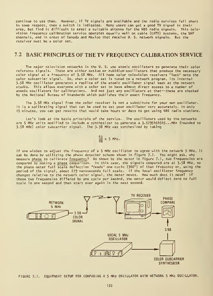
continue to use them. However, if TV signals are available and the radio services fall shortin some respect, then a switch is indicated. Many users can get a good TV signal in theirarea, but find it difficult to erect a suitable antenna for the NBS radio signals. This tele-vision frequency calibration service operates equally well on cable (CATV) systems, the UHFchannels, and in areas of Canada and Mexico that receive U. S. network signals. But thereceiver must be a color set.
7.2 BASIC PRINCIPLES OF THE TV FREQUENCY CALIBRATION SERVICE
The major television networks in the U. S. use atomic oscillators to generate their colorreference signals. These are either cesium or rubidium oscillators that produce the necessarycolor signal at a frequency of 3- 58 MHz. All home color television receivers "lock" onto the
color subcarrier signal. So, when a color set is tuned to a network program, its internal
3.58 MHz oscillator generates a replica of the atomic oscillator signal back at the networkstudio. This allows everyone with a color set to have almost direct access to a number ofatomic oscillators for calibrations. And not just any oscillators at that— these are checkedby the National Bureau of Standards which publishes their exact frequency.
The 3> 58 MHz signal from the color receiver is not a substitute for your own oscillator.It is a calibrating signal that can be used to set your oscillator very accurately. In only
15 minutes, you can get results that would take hours or days to get using NBS radio stations.
Let's look at the basic principle of the service. The oscillators used by the networksare 5 MHz units modified to include a synthesizer to generate a 3- 5795^5^5^5 • . .MHz (rounded to
3.58 MHz) color subcarrier signal. The 3- 58 MHz was synthesized by taking
§x5MHz.
If one wishes to adjust the frequency of a 5 MHz oscillator to agree with the network 5 MHz, it
can be done by utilizing the phase detector scheme shown in figure 7.\. You might ask, why
measure phase to calibrate frequency ? As shown by the meter in figure 7-1, two frequencies are
compared by making a phase comparison. In this case, the signals compared are at 3> 58 MHz, so
the phase meter full scale deflection "reads" one cycle (360°) of that frequency or, using the
period of the signal, about 279 nanoseconds full scale. If the local oscillator frequency
changes relative to the network color signal, the meter moves. How much does it move? If
those two frequencies differed by one cycle per second, the meter would deflect zero to full
scale in one second and then start over again in the next second.
NETWORK5 MHz
3.58
COLORSIGNAL
IV
TV RECEIVERPHASE
COMPARE
3.58
LOCAL 5 MHzOSCILLATOR
COLOR SUBCARRIER
SYNTHESIZER
FIGURE 7.1. EQUIPMENT SETUP FOR COMPARING A 5 MHz OSCILLATOR WITH NETWORK 5 MHz OSCILLATOR.
122
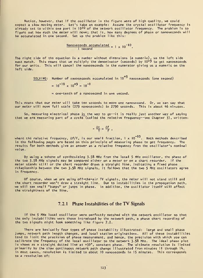
Notice, however, that if the oscillator in the figure were of high quality, we couldexpect a slow moving meter. Let's take an example: Assume the crystal oscillator frequency is
already set to within one part in 10'0 of the network oscillator frequency. The problem is to
figure out how much the meter will move; that is, how many degrees of phase or nanoseconds will
be accumulated in one second. Set up the problem like this:
Nanoseconds accumulated , ,«- 10
: 3 = 1 x 101 second
The right side of the equation is a number without dimensions (a numeric), so the left sidemust match. This means that we multiply the denominator (seconds) by 10+9 to get nanosecondsfor our units. This will cancel the nanoseconds in the numerator giving us a numeric on the
left side.
SOLVING : Number of nanoseconds accumulated in 10 nanoseconds (one second)
= 10-'° x 10+9
= 10" 1
= one-tenth of a nanosecond in one second.
This means that our meter will take ten seconds to move one nanosecond. Or, we can say that
our meter will move full scale (279 nanoseconds) in 2790 seconds. This is about 46 minutes.
So, measuring electrical phase j_s_ the way to go— it is really just another way of sayingthat we are measuring part of a cycle (called the relative frequency-see Chapter 3), written:
At Af
T f'
where the relative frequency, Af/f, is our small fraction, 1 x 10 . Both methods describedin the following pages are based on this principle of measuring phase to get frequency. Theresults for both methods give an answer as a relative frequency from the oscillator's nominalvalue.
By using a scheme of synthesizing 3.58 MHz from the local 5 MHz oscillator, the phase ofthe two 3.58 MHz signals may be compared either on a meter or on a chart recorder. If themeter stands still or the chart recorder draws a straight line, indicating a fixed phaserelationship between the two 3-58 MHz signals, it follows that the two 5 MHz oscillators agreein frequency.
Of course, when we are using off-the-air TV signals, the meter will not stand still andthe chart recorder won't draw a straight line. Due to instabilities in the propagation path,we will see small "bumps" or jumps in phase. In addition, the oscillator itself will affectthe straightness of the line.
7.2. 1 Phase Instabilities of the TV Signals
If the 5 MHz local oscillator were perfectly matched with the network oscillator so thatthe only instabilities were those introduced by the network path, a phase chart recording ofthe two signals might look something like figure 7.2.
There are basically four types of phase instability illustrated: large and small phasejumps, network path length changes, and local station originations. All of these instabilitiestend to limit the precision of phase measurement, and hence, the precision with which you cancalibrate the frequency of the local oscillator to the network 3-58 MHz. The ideal phase plotis shown as a straight dotted line at +30°, constant phase. The ultimate resolution is limitedprimarily by the slow continuous network path change illustrated from minutes 11 through \k.
In most cases, resolution is limited to about 10 nanoseconds in 15 minutes. This correspondsto a resolution of:
123
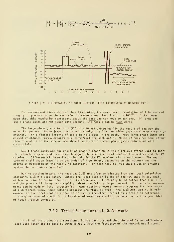
10 ns 10 ns
5 min 900 s
10
0.9 x I03
s
= 1 10
LARGE.PHASE JUMPS LOCAL STATION
ORIGINATION
DEALPHASE PLOT
SLOWCONTINUOUS NETWORK
PATH CHANGE
FIGURE 7.2 ILLUSTRATION OF PHASE INSTABILITIES INTRODUCED BY NETWORK PATH.
For measurement times shorter than 15 minutes, the measurement resolution will be reducedroughly in proportion to the reduction in measurement time; i.e., 1 x 10"'° in 1.5 minutes.Note that this resolution represents about the best one can hope to achieve. If large andsmall phase jumps are not taken into account, the result can be much worse.
The large phase jumps (up to + 90° or + 70 ns) are primarily the result of the way thenetworks operate. Phase jumps are caused by switching from one video tape machine or camera toanother, with different lengths of cable being placed in the path. Most large phase jumps arecaused by changes from a program to a commercial and back again. Using TV requires some atten-tion to what is on the screen--one should be alert to sudden phase jumps coincident withcommercial s.
Small phase jumps are the result of phase distortion in the microwave system used to carry
the network programs and to multipath signals between the local station transmitter and the TV
receiver. Differential phase distortion within the TV receiver also contributes. The magni-tude of small phase jumps is on the order of 1 to 10 ns, depending on the network and the
degree of multipath at the receiving location. For best results, you should use an antennasystem that minimizes "ghosts."
During station breaks, the received 3-58 MHz often originates from the local television
station's 3.58 MHz oscillator. Unless the local station is one of the few that is equipped
with a rubidium or cesium oscillator, its frequency will probably be no better than 1 x 10"',
and the phase will change more rapidly, about one full cycle per second. No precision measure-ments can be made on local programming. Many stations record network programs for rebroadcast
at a different time. When network programs are "tape delayed," the 3.58 MHz, again, is ref-
erenced to the local station's oscillator and is therefore invalid as a precision reference.
In any given area of the U. S., a few days of experience will provide a user with a good idea
of local program schedules.
7.2.2 Typical Values for the U. S. Networks
In all of the preceding discussions, it has been assumed that the goal is to calibrate a
local oscillator and to make it agree exactly with the frequency of the network oscillators.
24
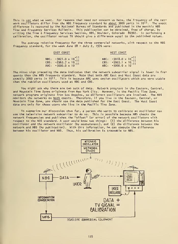
This is not what we want. For reasons that need not concern us here, the frequency of the net-
work oscillators differ from the NBS frequency standard by about 3000 parts in 10". The exactdifference is measured by the National Bureau of Standards and published in the monthly NBS
Time and Frequency Services Bulletin. This publication can be obtained, free of charge, by
writing the Time 6 Frequency Services Section, NBS, Boulder, Colorado 80302. In performing a
calibration, the oscillator versus TV should give a difference equal to the published values.
The average relative frequency for the three commercial networks, with respect to the NBS
frequency standard, for the week June 28 - July 2, 1976 were:
NBC
CBSABC
EAST COAST
-3021.0 x
-2963.7 x-3000.0 x
-11
-11
-11
NBC
CBS
ABC
WEST COAST
-3018.0 x 10
-3003.1 x 10
-3000.0 x 10
-11
-11
11
The minus sign preceding the data indicates that the network subcarrier signal is lower in fre-
quency than the NBS frequency standard. Note that both ABC East and West Coast data areexactly 3000 parts in 1
11 _ This is because ABC uses cesium oscillators which are more stable
than the rubidium oscillators used at NBC and CBS.
You might ask why there are two sets of data. Network programs in the Eastern, Central,and Mountain Time Zones originate from New York City. However, in the Pacific Time Zone,network programs originate from Los Angeles, so different oscillators are involved. The NBS
monitors the networks on both coasts. Therefore, if you live in the Eastern, Central, orMountain Time Zone, you should use the data published for the East Coast. The West Coastdata are only for those users who live in the Pacific Time Zone.
To summarize our discussion thus far, a person who wants to calibrate an oscillator canuse the television network subcarrier to do so. This is possible because NBS checks thenetwork frequencies and publishes the "offset" (or error) of the network oscillators withrespect to the NBS standard. A user would know two things: (1) the difference between his
oscillator and the network oscillator (by measurement), and (2) the difference between the
network and NBS (by publication). With this information, he can compute the differencebetween his oscillator and NBS. Thus, his calibration is traceable to NBS.
ATOMIC04CILLAT0E
NETWORK.<3TUDI0
^U^ l^ 1
>>) ) ,: nj
)
M&4 DATA
~jj*j«
informationconsultation DATA +
TV 4I6NAL =CALIBRATION
MFGrDEVELOPS flOMMER&IAL EQUIPMENT
125
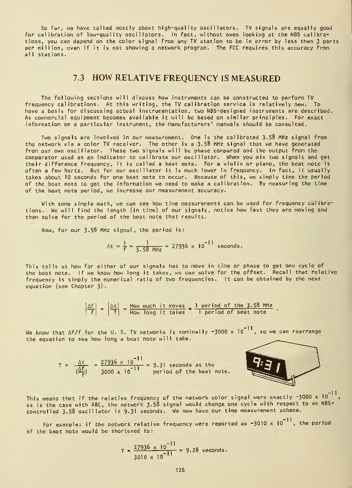
So far, we have talked mostly about high-quality oscillators. TV signals are equally good
for calibration of low-quality oscillators. In fact, without even looking at the NBS calibra-tions, you can depend on the color signal from any TV station to be in error by less than 3 parts
per million, even if it is not showing a network program. The FCC requires this accuracy fromall stations.
7.3 HOW RELATIVE FREQUENCY IS MEASURED
The following sections will discuss how instruments can be constructed to perform TV
frequency calibrations. At this writing, the TV calibration service is relatively new. To
have a basis for discussing actual instrumentation, two NBS-designed instruments are described.As commercial equipment becomes available it will be based on similar principles. For exact
information on a particular instrument, the manufacturers' manuals should be consulted.
Two signals are involved in our measurement. One is the calibrated 3-58 MHz signal from
the network via a color TV receiver. The other is a 3-58 MHz signal that we have generated
from our own oscillator. These two signals will be phase compared and the output from the
comparator used as an indicator to calibrate our oscillator. When you mix two signals and get
their difference frequency, it is called a beat note. For a violin or piano, the beat note is
often a few hertz. But for our oscillator it is much lower in frequency. In fact, it usually
takes about 10 seconds for one beat note to occur. Because of this, we simply time the period
of the beat note to get the information we need to make a calibration. By measuring the time
of the beat note period, we increase our measurement accuracy.
With some simple math, we can see how time measurements can be used for frequency calibra-
tions. We will find the length (in time) of our signals, notice how fast they are moving and
then solve for the period of the beat note that results.
Now, for our 3 • 58 MHz signal, the period is:
At = -^ = 1
f 3.58 MHz= 27936 x lO"
11seconds
This tells us how far either of our signals has to move in time or phase to get one cycle of
the beat note. If we know how long it takes, we can solve for the offset. Recall that relative
frequency is simply the numerical ratio of two frequencies. It can be obtained by the next
equation (see Chapter 3)
•
How much it moves _ 1 period of the 3-58 MHz
How long it takes "1 period of beat note
We know that Af/f for the U. S. TV networks is nominally -3000 x 10
the equation to see how long a beat note will take.
•11so we can rearrange
T =
<4f>
At _ 27936 x 10
3000 x 10~
•11
9.3' seconds as the
period of the beat note.
This means that if the relative frequency of the network color signal were exactly -3000 x 10
as is the case with ABC, the network 3. 58 signal would change one cycle with respect to an NBS-
controlled 3.58 oscillator in 9.31 seconds. We now have our time measurement scheme.
For example: if the network relative frequency were reported as -301 x 10 , the period
of the beat note would be shortened to:
11
T = 27936 x 10•11
3010 x 10-11
= 9.28 seconds,
126
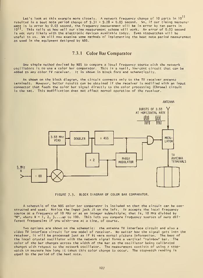
Let's look at this example more closely. A network frequency change of 10 parts in 10
resulted in a beat note period change of 9-31 ~ 9.28 = 0.03 second. So, if our timing measure-ment is in error by 0.03 second, the frequency measurement will be in error by ten parts in
10''. This tells us how well our time measurement scheme will work. An error of 0.03 second
is not very likely with the electronic devices available today. Even stopwatches will be
useful to us. We will now examine some methods of implementing the beat note period measurementas used in the equipment designed by NBS.
7.3.1 Color Bar Comparator
One simple method devised by NBS to compare a local frequency source with the networkoscillators is to use a color bar comparator. This is a small, low-cost circuit that can be
added to any color TV receiver. It is shown in block form and schemat ical ly
.
As shown on the block diagram, the circuit connects only to the TV receiver antennaterminals. However, better results can be obtained if the receiver is modified with an input
connector that feeds the color bar signal directly to the color processing (Chroma) circuitin the set. This modification does not affect normal operation of the receiver.
ANTENNA
BURSTS OF 3.58 VAT HORIZONTAL RATE
3.58 MHzVCXO
5 MHz
N
D0UBLER 455 TO
PHASEMODULATOR
MODU-LATOR
TV
ANTENNATERMINALS
FIGURE 7-3. BLOCK DIAGRAM OF COLOR BAR COMPARATOR.
A schematic of the NBS color bar comparator is included so that the circuit can be con-structed and used. Notice the input jack Jl on the left. It accepts the local frequencysource at a frequency of 10 MHz or at an integer submultiple; that is, 10 MHz divided by
"N", where N = 1, 2, 3.. ..up to 100. This lets you compare frequency sources of many dif-ferent frequencies if you wish—one at a time, of course.
Two options are shown on the schematic: the antenna TV interface circuit and also a
video TV interface circuit for one model of receiver. No matter how the signal gets into thereceiver, it will be processed just as if it were normal picture information. The beat of
the local crystal oscillator with the network signal forms a vertical "rainbow" bar. The
color of the bar changes across the width of the bar as the oscillator being calibratedchanges with respect to the network oscillator. The measurement consists of using a stop-
watch to measure how long it takes this color change to occur. The stopwatch reading is
equal to the period of the beat note.
127
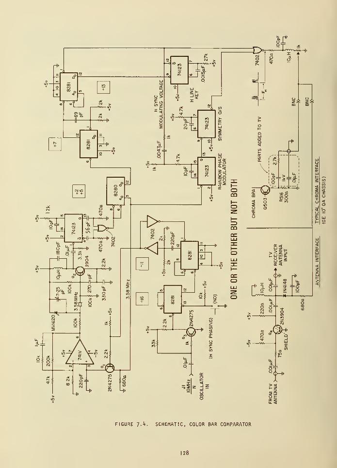
FIGURE l.k. SCHEMATIC, COLOR BAR COMPARATOR
128
To use the color bar system for oscillator calibration, tune the receiver to a network
color program, and set the oscillator to be calibrated so that the rainbow appears to move
across the bar from right to left through a complete color cycle (from red to green to blue
and back to red) in about 10 seconds. The color bar itself moves slowly across the screen
from right to left. If the frequency of your oscillator is far off, the colors in the
rainbow pattern will change very rapidly and the entire bar will move rapidly across the
screen in the direction of the color changes. The bar can be positioned to the middle of the
screen by the pushbutton labeled "Horizontal Sync Phasing."
With the rainbow repeating colors in about 10 seconds,
carefully adjust the crystal oscillator until the period is:
T = 27936 x 10•11
NBS published data for network being viewedseconds
.
If possible, check more than one network to increase the
confidence in calibration. Also, by measuring over ten beat
note periods, the effect of reaction time with the stopwatch
will be reduced. Recall that for 1 period, an error of 0.03 second corresponds to a frequency
error of 10 parts in 10^. For ten periods, a measurement error of 0.03 second will result in
a frequency error of 1 part in lO''.
As mentioned before, the rainbow will be of higher quality if the signal is connected into
the receiver as a video signal. The improvement is due to the fact that antenna injection alsomodulates the received audio carrier. This results in a visible beat note that constantlychanges with the audio content of the program. The other example circuit shown connects the
signal directly into the Chroma bandpass amplifier. The rainbow is then nearly perfect.
7.3.2 The NBS System 358 Frequency Measurement Computer
For those users who require accuracies approaching 1 part in 10 , another calibrationmethod is available. The System 358 Frequency Measurement Computer (FMC) computes and displaysthe oscillator's relative frequency directly on the TV screen. The user simply turns on theunit and waits for 15 minutes. He then comes back, reads off 10 values, and averages them to
obtain the result. Other versions of the FMC are commercially available that use a separatedigital display rather than the TV screen.
The FMC automatically performs the operation of measuring the period of the 3-58 MHz beatnote "T," computing At/T, scaling the result for readout in parts in 10^, and displaying theone- and ten-period averages on the TV screen. Readout is a series of 't-digit numbers, represent-ing the relative frequency between the oscillator being calibrated and the atomically controlledcolor subcarrier. By referring to network data published monthly in the NBS Time and FrequencyServices Bulletin, a user of the FMC can set his oscillator to agree with the NBS standard to
better than 1 part in 10'°* in five minutes and 3 parts in 10'1 in fifteen minutes. Radiomethods of calibrating oscillators traceable to NBS require several days of "averaging" to
achieve this resolution. Measurement uncertainties as a function of averaging time that may be
reasonably be expected are:
AVERAGING TIME:
MEASUREMENT UNCERTAINTY:
10 seconds 100 seconds 15 minutes
3 x 10⁻¹⁰
6 x 10-11
2 x 10¹¹
30 minutes
1 .5 x 10-11
2h hours
6 x 10" 12
When making network frequency comparisons, the FMC will also accept as input any oscillatorwhose frequency is 10/N MHz, where "N" is any integer from 1 to 100. The highest availablefrequency should be used when there is a choice.
The FMC consists of a 5- inch color TV receiver with an additional electronics package
mounted to its base. Readout for the FMC is on the TV screen, with two columns of ten4-digit numbers, and an additional analog "phase cursor."
129
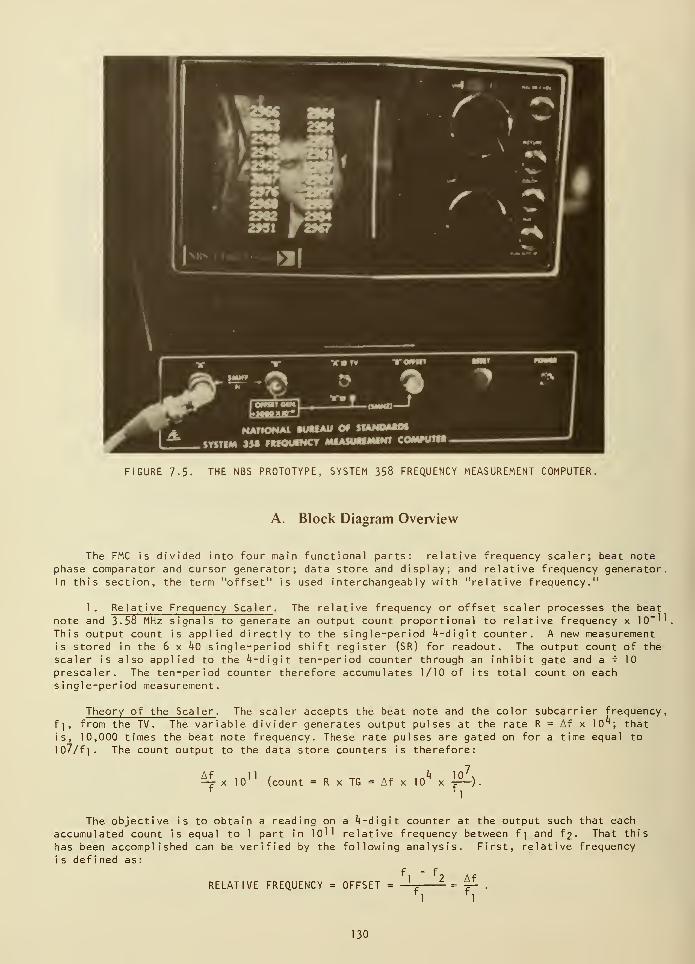
FIGURE 7-5. THE NBS PROTOTYPE, SYSTEM 358 FREQUENCY MEASUREMENT COMPUTER.
A. Block Diagram Overview
The FMC is divided into four main functional parts: relative frequency scaler; beat notephase comparator and cursor generator; data store and display; and relative frequency generator.In this section, the term "offset" is used interchangeably with "relative frequency."
1. Relative Frequency Scaler . The relative frequency or offset scaler processes the beat
note and 3.58 MHz signals to generate an output count proportional to relative frequency x 10"''
This output count is applied directly to the single-period 4-digit counter. A new measurementis stored in the 6 x ^0 single-period shift register (SR) for readout. The output count of the
scaler is also applied to the *»-digit ten-period counter through an inhibit gate and a * 10
prescaler. The ten-period counter therefore accumulates 1/10 of its total count on eachsingle-period measurement.
Theory of the Scaler . The scaler accepts the beat note and the color subcarrier frequency,
f|, from the TV. The variable divider generates output pulses at the rate R = Af x 10^; that
is, 10,000 times the beat note frequency. These rate pulses are gated on for a time equal to
107/f|. The count output to the data store counters is therefore:
Af10
11(count = R x TG = Af x 10
k
f>The objective is to obtain a reading on a '-digit counter at the output such that each
accumulated count is equal to 1 part in 10^' relative frequency between f] and f£. That this
has been accomplished can be verified by the following analysis. First, relative frequency
i s defined as
:
RELATIVE FREQUENCY = OFFSET = 1 Af
f.
130
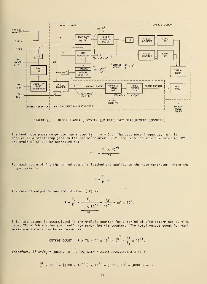
3.58 MHzFROM TV
OFFSETOUTPUT
r
5 MHzPLL
+ 3000x 10""
OFFSETGENERATOR
OFFSET GENERATOR
OFFSET SCALER
(f|)
(f,)
If.)
PHASECOMPARE
I07
TIME GATE
Tr-J£TG"f,
RATEGENERATOR
r4
INHIBIT
10 PERIODCOUNT
!=o
-E3t
(R)-if x I04
PERIODCOUNT (P)
(P) = -
OUTPUT _if|0
ll
f,xlO-"C0UNT
" fi
Af
STORE a DISPLAY
4 DIGITCOUNTER
6x40SR
4 DIGITCOUNTER
ANALOG PHASE
"BEAT NOTE"Af=f,-f,
PHASE COMPARE a PHASE CURSOR
VARIABLEPERIOD0/S
FIXEDPERIOD0/S
(30-40^.s) (0.5/xs)
H SYNCFROM TV
6x40SR
PHASE CURSOR
DISPLAY
LOGIC
VIDEOMIXER
DISPLAYVIDEOTO TV
FIGURE 7-6. BLOCK DIAGRAM, SYSTEM 358 FREQUENCY MEASUREMENT COMPUTER.
The beat note phase comparator generates fj ~ ^1~ ^f. The beat note frequency, Af , is
applied as a start-stop gate to the period counter, "P." The total count accumulated in "P" in
one cycle of Af can be expressed as:
-kf x 10
iipu _ _JAf
For each cycle of Af , the period count is latched and applied to the rate generator, where theoutput rate is
R =
The rate of output pulses from divider (tP) is:
R =P-1 Af
nr—
nrf. x 10 10
Af
Af x 10 .
This rate output is accumulated in the '-digit counter for a period of time determined by timegate, TG, which enables the "and" gate preceding the counter. The total output count for eachmeasurement cycle can be expressed as:
OUTPUT COUNT = R x TG = Af x 1
0**x ^- = ^- x 1
]'
.
Therefore, if Af/f. = 3000 x 10 , the output count accumulated will be
Af in 11[3000 x lO
-11] x 10
11= 3000 x 10° = 3000 counts.
131
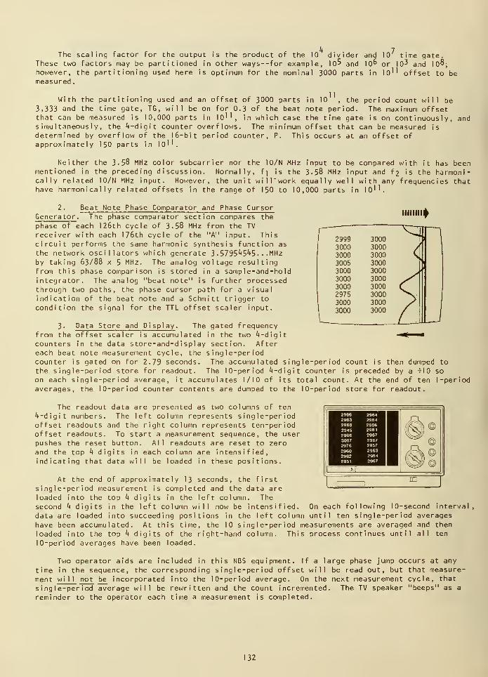
Z, 7The scaling factor for the output is the product of the 10 divider and 10 time gate.
These two factors may be partitioned in other ways--for example, 10^ and 10^ or 10^ and lo8;
however, the partitioning used here is optimum for the nominal 3000 parts in 10*' offset to bemeasured
.
With the partitioning used and an offset of 3000 parts in 10 , the period count will be
3,333 and the time gate, TG , will be on for 0.3 of the beat note period. The maximum offsetthat can be measured is 10,000 parts in 10'^, in which case the time gate is on continuously, andsimultaneously, the 4-digit counter overflows. The minimum offset that can be measured is
determined by overflow of the 16-bit period counter, P. This occurs at an offset ofapproximately 150 parts in 10''.
Neither the 3.58 MHz color subcarrier nor the 10/N MHz input to be compared with it has beenmentioned in the preceding discussion. Normally, f] is the 3 • 58 MHz input and f2 is the harmoni-cally related 10/N MHz input. However, the unit will" work equally well with any frequencies thathave harmonically related offsets in the range of 150 to 10,000 parts in lo'^.
IIIIIIII+2. Beat Note Phase Comparator and Phase Cursor
Generator . The phase comparator section compares the
phase of each 126th cycle of 3.58 MHz from the TV
receiver with each 176th cycle of the "A" input. Thiscircuit performs the same harmonic synthesis function as
the network oscillators which generate 3 • 5735^5^5 •• -MHz
by taking 63/88 x 5 MHz. The analog voltage resultingfrom this phase comparison is stored in a sampl e-and-holdintegrator. The analog "beat note" is further processedthrough two paths, the phase cursor path for a visualindication of the beat note and a Schmitt trigger to
condition the signal for the TTL offset scaler input.
3. Data Store and Display . The gated frequencyfrom the offset scaler is accumulated in the two '-digitcounters in the data store-and-d isplay section. Aftereach beat note measurement cycle, the single-periodcounter is gated on for 2.79 seconds. The accumulated single-period count is then dumped to
the single-period store for readout. The 10-period '-digit counter is preceded by a t10 soon each single-period average, it accumulates 1/10 of its total count. At the end of ten 1-periodaverages, the 10-period counter contents are dumped to the 10-period store for readout.
2999 3000
3000 30003000 3000
3005 3000
3000 3000
3000 3000
3000 3000
2975 3000
3000 3000
3000 3000
The readout data are presented as two columns of ten'-digit numbers. The left column represents single-periodoffset readouts and the right column represents ten-periodoffset readouts. To start a measurement sequence, the userpushes the reset button. All readouts are reset to zeroand the top h digits in each column are intensified,indicating that data will be loaded in these positions.
At the end of approximately 13 seconds, the first ID
single-period measurement is completed and the data are —
•
—~~
loaded into the top k digits in the left column. Thesecond k digits in the left column will now be intensified. On each following 10-second interval,
data are loaded into succeeding positions in the left column until ten single-period averageshave been accumulated. At this time, the 10 single-period measurements are averaged and then
loaded into the top k digits of the right-hand column. This process continues until all ten
10-period averages have been loaded.
Two operator aids are included in this NBS equipment. If a large phase jump occurs at any
time in the sequence, the corresponding single-period offset will be read out, but that measure-
ment will not be incorporated into the 10-period average. On the next measurement cycle, that
single-period average will be rewritten and the count incremented. The TV speaker "beeps" as a
reminder to the operator each time a measurement is completed.
32
B. Use of FMC with Unstable Crystal Oscillators
The FMC is primarily intended to calibrate oscillators with stability of better than 1 partin lO? per day. In fact, if the oscillator being calibrated will not hold still to better than1 part in 107 (+ 10,000 parts in lO'M, the digital readout cannot be used. About the best onecan do with a really poor-quality oscillator is make the cursor "stand still" momentarily.
If the cursor moves less than one cycle each three seconds, then the oscillator is within1 part in 10' of the color subcarrier. By switching between networks, one can obtain a "concensus;"however, there is no way to really verify if the subcarrier is originating from a network, as canbe done when checking a good oscillator.
The FCC requires all stations to maintain 3-5795^5. • .MHz + 10 Hz on their subcarriers, so by
comparing with several stations, one is assured of being within 3 parts in 10°. If the oscillatorbeing calibrated is stable to 0.001% (1 part in 10->), it is close enough.
7.4 GETTING GOOD TV CALIBRATIONS
Although the frequency calibration service using TV reduces the labor of calibrating an
oscillator, it does not relieve the user of the responsibility of verifying that "good" dataare actually being processed. The user must be sure that the station being used is actuallytransmitting network-originated programs.
At the present time, data for three networks are available from NBS. The easiest thing to
do is to take successive readings, if possible, on all three networks for 1.5 minutes each andverify that they differ relative to each other by approximately the correct amount. Nominally,on the East Coast, CBS operates at -3000 parts in 10^ ] and NBC operates at -3020 parts in 10 1 '.
ABC operates at exactly -3000 parts in 10 11.
Assume relative frequency readings were taken with the following correct results:
11
11
11
ABC: -3131 x 10
NBC: -3150 x 10
CBS: -3130 x 10
The readings are consistent from one network to another. If one of the three had differedradically from its correct relative value, we could assume that the station involved was on
local programming. For example, if the reading for NBC were -2^60, then the NBC station wouldnot be used at that time.
Measurements must be made only when network-originated programs are on the air. Networkstations in the Eastern, Central, and Pacific time zones typically carry 10 to ]k hours of
network-originated programs per day. The Mountain time zone carries about four hours per day.
It should be noted that network-originated programs arenot necessarily "live" programs (such as football or basket-ball games). It simply means that the programs are originatedfrom the network centers in either Los Angeles or New York City
and are not tape delayed by the local stations. Programsoriginating at the local stations (such as the channel k newsas opposed to CBS Evening News) cannot be used.
The best choices are the daytime soap operas and quiz
shows. These usually are daily programs and originate fromthe New York and/or Los Angeles network centers. Weeklyevening programs are usual ly network-originated except in
the Mountain Time Zone. Once the programming schedule in
any given city is identified, a log can be made to indicate
when measurements can be made.
133
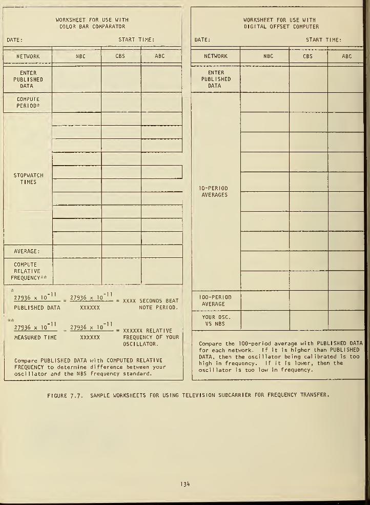
WORKSHEET FOR USE WITHCOLOR BAR COMPARATOR
DATE: START TIME:
NETWORK NBC CBS ABC
ENTERPUBLISHED
DATA
COMPUTEPERIOD*
STOPWATCHTIMES
AVERAGE:
COMPUTERELATIVE
FREQUENCY**
27936 x lo"11
= 27936 x Itf11
= xxxx SEC0N[)S BEAT
PUBLISHED DATA XXXXXX NOTE PERIOD.
27936 x 10' 11
= 27936 x l<fn
= mm RELAT|yEMEASURED TIME XXXXXX FREQUENCY OF YOUR
OSCILLATOR.
Compare PUBLISHED DATA with COMPUTED RELATIVEFREQUENCY to determine difference between your
oscillator and the NBS frequency standard.
FIGURE 7.7. SAMPLE WORKSHEETS FOR USING
WORKSHEET FOR USE WITHDIGITAL OFFSET COMPUTER
DATE: START TIME:
NETWORK NBC CBS ABC
ENTERPUBLISHED
DATA
10-PERIODAVERAGES
lOO-PERIODAVERAGE
YOUR OSC.
VS NBS
Compare the 100-period average with PUBLISHED DATA
for each network. If it is higher than PUBLISHED
DATA, then the oscillator being calibrated is too
high in frequency. If it is lower, then the
oscillator is too low in frequency.
.EVISION SUBCARR IER FOR FREQUEh CY TRANSFER
134
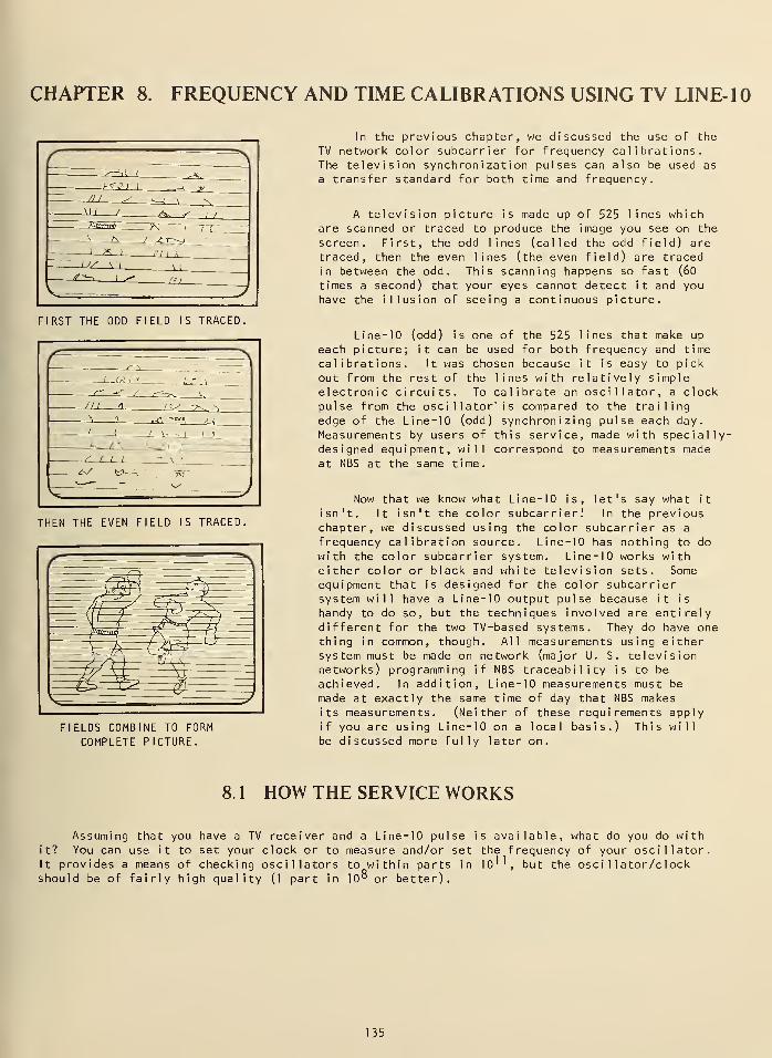
CHAPTER 8. FREQUENCY AND TIME CALIBRATIONS USING TV LINE- 10
c~ "Ar~^K i ,Jt
>.«-.SI | -A' ^/H s '—1 \ -N
\\i /<**- /- / /„.„
=e r-rr Z_Z
1 X 1 '•' ' i
,S
us \-\\ i
//^ 1^< r/i
vl 3^
FIRST THE ODD FIELD IS TRACED.
>—
i
-T^T— c /-'.v-v '•- a
s- ~r / ^-->, -L
II 1 /\ /C^ ->v ^•\ '/ ^\ ""BO". J 1
/ 1 / \. - 1 1 1
A. //\ ^J7\—7
S f 1 1 - V 1.
<6/_ t?—
,
... _^„
JL_^
THEN THE EVEN FIELD IS TRACED.
In the previous chapter, we discussed the use of the
TV network color subcarrier for frequency calibrations.The television synchronization pulses can also be used as
a transfer standard for both time and frequency.
A television picture is made up of 525 lines whichare scanned or traced to produce the image you see on the
screen. First, the odd lines (called the odd field) aretraced, then the even lines (the even field) are traced
in between the odd. This scanning happens so fast (60
times a second) that your eyes cannot detect it and youhave the illusion of seeing a continuous picture.
Line-10 (odd) is one of the 525 lines that make up
each picture; it can be used for both frequency and time
calibrations. It was chosen because it is easy to pickout from the rest of the lines with relatively simpleelectronic circuits. To calibrate an oscillator, a clockpulse from the osci 1 lator' is compared to the trailingedge of the Line-10 (odd) synchronizing pulse each day.
Measurements by users of this service, made with specially-designed equipment, will correspond to measurements made
at NBS at the same time.
FIELDS COMBINE TO FORM
COMPLETE PICTURE.
Now that we know what Li
isn't. It isn't the color su
chapter, we discussed using t
frequency calibration source,with the color subcarrier sys
either color or black and whi
equipment that is designed fo
system will have a Line-10 ouhandy to do so, but the techndifferent for the two TV-basething in common, though. All
system must be made on networnetworks) programming if NBS
achieved. In addition, Line-made at exactly the same time
its measurements. (Neither o
if you are using Line-10 on a
be discussed more fully later
ne-10 is, let's say what it
bcarrier! In the previoushe color subcarrier as a
Line-10 has nothing to do
tern. Line-10 works withte television sets. Some
r the color subcarriertput pulse because it is
iques involved are entirelyd systems. They do have onemeasurements using either
k (major U. S. televisiontraceability is to be
10 measurements must be
of day that NBS makes
f these requirements applylocal bas is.) Thi s will
on
.
8. 1 HOW THE SERVICE WORKS
Assuming that you have a TV receiver and a Line-10 pulse is available, what do you do withit? You can use it to set your clock or to measure and/or set the frequency of your oscillator,It provides a means of checking oscillators to within partsshould be of fairly high quality (1 part in 10° or better).
10 1 ', but the oscillator/clock
135
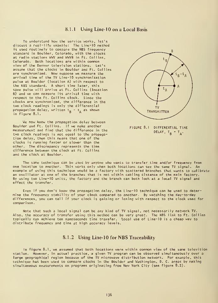
8. 1 . 1 Using Line- 1 on a Local Basis
To understand how the service works, let'sdiscuss a real-life example: The Line-10 methodis used routinely to compare the NBS frequencystandard in Boulder, Colorado, with the clocksat radio stations WWV and WWVB in Ft. Collins,Colorado. Both locations are within commonview of the Denver television stations. Let'sassume that the clocks in Boulder and Ft. Collinsare synchronized. Now suppose we measure thearrival time of the TV Line-10 synchronizationpulse at Boulder (location A) with respect to
the NBS standard. A short time later, thissame pulse will arrive at Ft. Collins (locationB) and we can measure its arrival time withrespect to the Ft. Collins clock. Since theclocks are synchronized, the difference in thetwo clock readings is only the differentialpropagation delay, written t
in f i gure 8.1.B
t. as shownA
We now know the propagation delay betweenBoulder and Ft. Collins. If we make anothermeasurement and find that the difference in the
two clock readings is not equal to the propaga-tion delay, then this means that one of the
clocks is running faster or slower than the
other. The discrepancy represents the time
difference between the clock at Ft. Collinsand the clock at Boulder.
FIGURE 8.1 DIFFERENTIAL TIMEDELAY, T D - T„.
' B A
The same technique can be used by anyone who wants to transfer time and/or frequency fromone location to another. This works only when both locations can see the same TV signal. Anexample of using this technique would be a factory with scattered branches that wants to calibratean oscillator at one of the branches that is not within cabling distance of the main factory.By using two Line-10 units, the factory and the branch can both look at a local TV signal andeffect the transfer.
Even if you don't know the propagation delay, the Line-10 technique can be used to deter-mine the frequency stability of your clock compared to another. By watching the day-to-daydifferences, you can tell if your clock is gaining or losing with respect to the clock used for
compar i son
.
Note that such a local signal can be any kind of TV signal, not necessarily network TV.
Also, the accuracy of transfer using this method can be very great. The NBS 1 i.nk to Ft. Collinstypically can achieve ten nanoseconds time transfer. Local use of Line-10 is a cheap way to
distribute frequency and time at high accuracy levels.
8.1.2 Using Line-10 for NBS Traceability
In figure 8.1, we assumed that both locations were within common view of the same televisionstation. However, in actual practice, a given TV program can be observed simultaneously over a
large geographical region because of the TV microwave distribution network. For example, this
technique has been used to compare clocks in the Boulder and Washington, D. C. areas by makingsimultaneous measurements on programs originating from New York City (see figure 8.2).
136
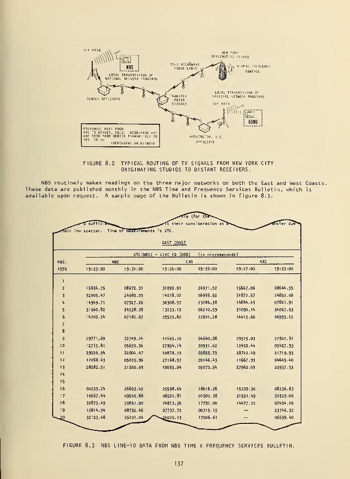
NEW YORKORIGINATING STUDIO
ATOMIC FREQUENCY
CONTROL
MICROWAVE PATH FROMNYC TO DENVER, COLO. 4000-6400 km*VHF PATH FROM DENVER TRANSMITTER TONBS 30 km
•DEPENDING ON NETWORK
WASHINGTON, O.C.
AFFILIATE
FIGURE 8.2 TYPICAL ROUTING OF TV SIGNALS FROM NEW YORK CITYORIGINATING STUDIOS TO DISTANT RECEIVERS.
NBS routinely makes readings on the three major networks on both the East and West Coasts,These data are published monthly in the NBS Time and Frequency Services Bulletin, which is
available upon request. A sample page of the Bulletin is shown in figure 8.3'
Ta (for tF
^*<*&~% u f f i cTSr ^*<^t- thei r cons Ideration ails r^nsfer due^
^»«(fle i r low scatter. 1 ime or measurements is UTC.
EAST COAST
AUG.
1976
UTC(NBS) - LINE 10 (ODD) (in mlcroseconc s)
NBC CBS ABC
19:25:00 19:31 :00 19:26:00 19:32:00 19:27:00 19=33:00
1
2 15694.75 08672.31 31093.91 24071.52 15667.06 08644.55
3 32005.47 24983.03 14018.02 06995.50 31872.57 24850.06
4 14949.71 07927.26 30308.97 23286.38 14884.43 07861.91
5 31260.82 24238.38 13233.12 06210.59 31090.14 24067.63
6
7
14205.24 07182.67 29523.82 22501 .28 14015.66 06993-12
8
9 29771.69 22749.24 11663.10 04640.58 29525.03 22502.51
10 12715.81 05693.36 27954.14 20931 .62 12450.44 05427.93
11 29026. 9*4 22004.47 10878.29 03855.73 28742.49 21719.93
12 1 2058.43 05035.96 27168.97 20146.43 11667.93 04645.40
13
I1*
28282.51 21260.09 10093.04 03070.54 27960.03 20937-53
15
16 00259.24 26603.42 25598.64 18616.28 15259.36 08236.83
17 16567.44 09542.88 08522.81 01500.38 31551.49 24529.06
18 32873.49 25851.00 24813.56 17791 .00 14477-22 07454.66
'9 15814.94 08792.46 07737.72 00715.15 -- 23746.32
U^20 32123.48 25101.04 /*""^4029. 13 17006.61 -- 06699.40
FIGURE 8.3 NBS LINE-10 DATA FROM NBS TIME & FREQUENCY SERVICES BULLETIN,
37
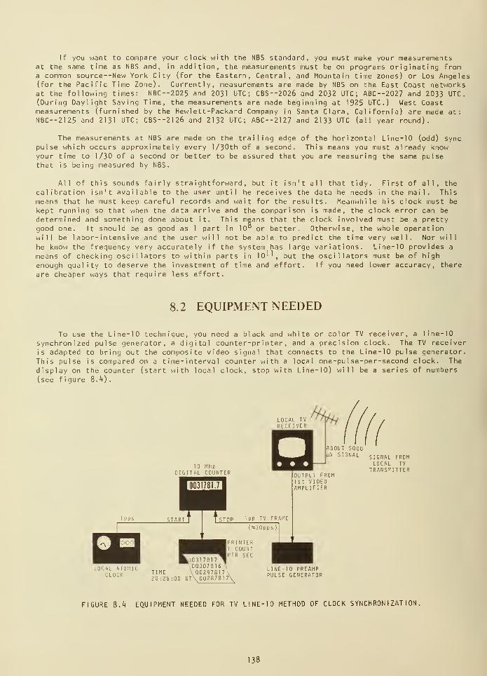
If you want to compare your clock with the NBS standard, you must make your measurementsat the same time as NBS and, in addition, the measurements must be on programs originating froma common source—New York City (for the Eastern, Central, and Mountain time zones) or Los Angeles(for the Pacific Time Zone). Currently, measurements are made by NBS on the East Coast networksat the following times: NBC--2025 and 2031 UTC ; CBS--2026 and 2032 UTC ; ABC--2027 and 2033 UTC.(During Daylight Saving Time, the measurements are made beginning at 1925 UTC.) West Coastmeasurements (furnished by the Hewlett-Packard Company in Santa Clara, California) are made at:
NBC--2125 and 2131 UTC; CBS--21 26 and 2132 UTC; ABC--2127 and 2133 UTC (all year round).
The measurements at NBS are made on the trailing edge of the horizontal Line-10 (odd) syncpulse which occurs approximately every 1 /30th of a second. This means you must already knowyour time to 1/30 of a second or better to be assured that you are measuring the same pulsethat is being measured by NBS.
All of this sounds fairly straightforward, but it isn't all that tidy. First of all, the
calibration isn't available to the user until he receives the data he needs in the mail. Thismeans that he must keep careful records and wait for the results. Meanwhile his clock must be
kept running so that when the data arrive and the comparison is made, the clock error can be
determined and something done about it. This means that the clock involved must be a prettygood one. It should be as good as 1 part in 10" or better. Otherwise, the whole operationwill be labor-intensive and the user will not be able to predict the time very well. Nor will
he know the frequency very accurately if the system has large variations. Line-10 provides a
means of checking oscillators to within parts in 10'', but the oscillators must be of high
enough quality to deserve the investment of time and effort. If you need lower accuracy, there
are cheaper ways that require less effort.
8.2 EQUIPMENT NEEDED
To use the Line-10 technique, you need a black and white or color TV receiver, a line-10
synchronized pulse generator, a digital counter-printer, and a precision clock. The TV receiver
is adapted to bring out the composite video signal that connects to the Line-10 pulse generator.
This pulse is compared on a t ime- i nterval counter with a local one-pul se-per-second clock. The
display on the counter (start with local clock, stop with Line-10) will be a series of numbers
(see f i gure 8.4) .
10 MHzDIGITAL COUNTER
lpps START
LOCAL ATOMICn nrK TIME \ °
20:25:00 UT\ 00287817
OUTPUT FROM1st VIDEOAMPLIFIER
LINE-10 PREAMPPULSE GENERATOR
SIGNAL FROMLOCAL TV
TRANSMITTER
FIGURE 8.4 EQUIPMENT NEEDED FOR TV LINE-10 METHOD OF CLOCK SYNCHRONIZATION.
38
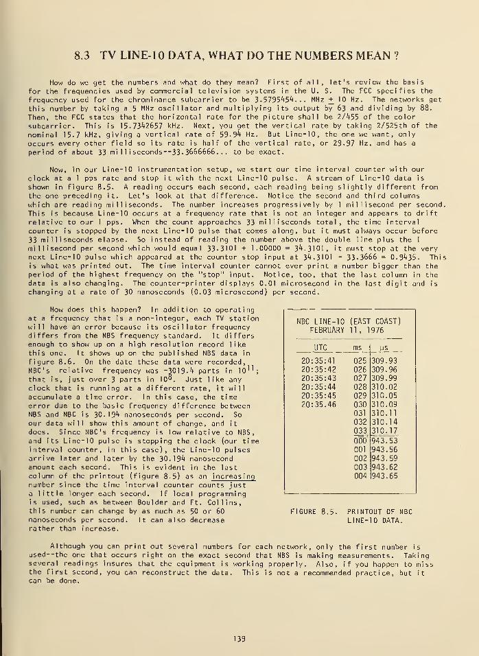
8.3 TV LINE-10 DATA, WHAT DO THE NUMBERS MEAN ?
How do we get the numbers and what do they mean? First of all, let's review the basis
for the frequencies used by commercial television systems in the U. S. The FCC specifies the
frequency used for the chrominance subcarrier to be 3-5795454... MHz +_ 10 Hz. The networks get
this number by taking a 5 MHz oscillator and multiplying its output by 63 and dividing by 88.
Then, the FCC states that the horizontal rate for the picture shall be 2/455 of the color
subcarrier. This is 15-7342657 kHz. Next, you get the vertical rate by taking 2/525th of the
nominal 15-7 kHz, giving a vertical rate of 59-94 Hz. But Line-10, the one we want, only
occurs every other field so its rate is half of the vertical rate, or 29-97 Hz, and has a
period of about 33 mi 1 1 i seconds--33- 3666666. . . to be exact.
Now, in our Line-10 instrumentation setup, we start our time in
clock at a 1 pps rate and stop it with the next Line-10 pulse. A st
shown in figure 8.5- A reading occurs each second, each reading bei
the one preceding it. Let's look at that difference. Notice the se
which are reading milliseconds. The number increases progressivelyThis is because Line-10 occurs at a frequency rate that is not an in
relative to our 1 pps. When the count approaches 33 milliseconds to
counter is stopped by the next Line-10 pulse that comes along, but i
33 milliseconds elapse. So instead of reading the number above themillisecond per second which would equal 33-3101 + 1.00000 = 3^-3101next Line-10 pulse which appeared at the counter stop input at 3^+ -31
is what was printed out. The time interval counter cannot ever prinperiod of the highest frequency on the "stop" input. Notice, too, t
data is also changing. The counter-printer displays 0.01 microseconchanging at a rate of 30 nanoseconds (0.03 microsecond) per second.
terval counter with ourream of Line-10 data is
ng slightly different fromcond and third columnsby 1 millisecond per second.teger and appears to drifttal , the time interval
t must always occur beforedouble 1 ine pi us the 1
, it must stop at the very01 - 33-3666 = 0.9435. Thist a number bigger than the
hat the last column in the
d in the last digit and is
How does this happen? In addition to operatingat a frequency that is a non-integer, each TV stationwill have an error because its oscillator frequencydiffers from the NBS frequency standard. It differsenough to show up on a high resolution record like
this one. It shows up on the published NBS data in
figure 8.6. On the date these data were recorded,NBC's relative frequency was -301 9 • ^ parts in 10^;that is, just over 3 parts in 10°. Just like anyclock that is running at a different rate, it willaccumulate a time error. In this case, the timeerror due to the basic frequency difference betweenNBS and NBC is 30.194 nanoseconds per second. So
our data will show this amount of change, and it
does. Since NBC's frequency is low relative to NBS,
and its Line-10 pulse is stopping the clock (our timeinterval counter, in this case), the Line-10 pulsesarrive later and later by the 30.194 nanosecondamount each second. This is evident in the lastcolumn of the printout (figure 8.5) as an increas ing
number since the time interval counter counts justa little longer each second. If local programmingis used, such as between Boulder and Ft. Collins,this number can change by as much as 50 or 60
nanoseconds per second. It can also decreaserather than increase.
NBC LINE-10 (EAST COAST)
FEBRUARY 11 , 1976
UTC ms ys
20:35:41 025 309.9320:35:42 026 309.9620:35:43 027 309.9920:35:44 028 310.0220:35:45 029 310.0520:35.46 030 310.09
031 310.11
032 310.14033 310.17
000 943.53001 943.56002 943.59003 943.62004 943.65
FIGURE 8.5- PRINTOUT OF NBCLINE-10 DATA.
Although you can print out several numbers for each network, only the first number is
used— the one that occurs right on the exact second that NBS is making measurements. Takingseveral readings insures that the equipment is working properly. Also, if you happen to missthe first second, you can reconstruct the data. This is not a recommended practice, but it
can be done.
139
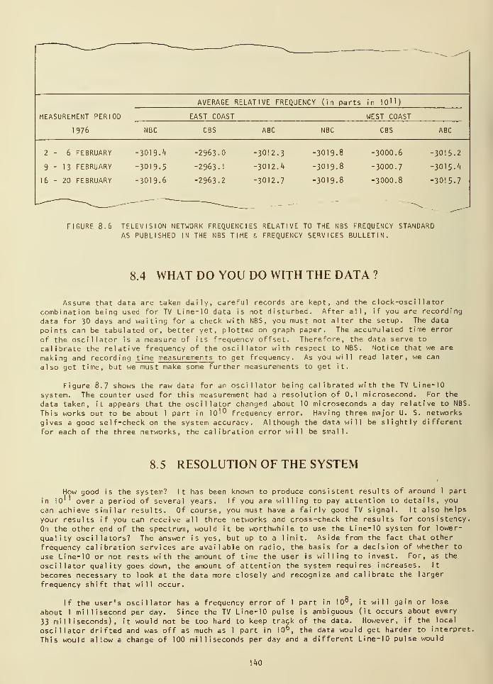
AVERAGE RELATIVE FREQUENCY (in parts in 10")
MEASUREMENT PERIOD
1976
EAST COAST WEST COAST
NBC CBS ABC NBC CBS ABC
2-6 FEBRUARY
9-13 FEBRUARY
6-20 FEBRUARY
301 9-
^
-2963.0 -3012.3 -3019.8 -3000.6 -3015.2
3019.5 -2963.I -3012. k -3019.8 -3000.7 -3015. k
3019.6 -2963.2 -3012.7 -3019.8 -3000.8 -3015.7
FIGURE 8.6 TELEVISION NETWORK FREQUENCIES RELATIVE TO THE NBS FREQUENCY STANDARD
AS PUBLISHED IN THE NBS TIME & FREQUENCY SERVICES BULLETIN.
8.4 WHAT DO YOU DO WITH THE DATA ?
Assume that data are taken daily, careful records are kept, and the clock-oscillator
combination being used for TV Line-10 data is not disturbed. After all, if you are recording
data for 30 days and waiting for a check with NBS, you must not alter the setup. The data
points can be tabulated or, better yet, plotted on graph paper. The accumulated time error
of the oscillator is a measure of its frequency offset. Therefore, the data serve to
calibrate the relative frequency of the oscillator with respect to NBS. Notice that we are
making and recording t ime measurements to get frequency. As you will read later, we can
also get time, but we must make some further measurements to get it.
Figure 8.7 shows the raw data for an oscillator being calibrated with the TV Line-10
system. The counter used for this measurement had a resolution of 0.1 microsecond. For the
data taken, it appears that the oscillator changed about 10 microseconds a day relative to NBS.
This works out to be about 1 part in 10'0 frequency error. Having three major U. S. networks
gives a good self-check on the system accuracy. Although the data will be slightly different
for each of the three networks, the calibration error will be small.
8.5 RESOLUTION OF THE SYSTEM
How good is the system? It has been known to produce consistent results of around 1 part
in 10 over a period of several years. If you are willing to pay attention to details, you
can achieve similar results. Of course, you must have a fairly good TV signal. It also helps
your results if you can receive all three networks and cross-check the results for consistency.
On the other end of the spectrum, would it be worthwhile to use the Line-10 system for lower-
quality oscillators? The answer is yes, but up to a limit. Aside from the fact that other
frequency calibration services are available on radio, the basis for a decision of whether to
use Line-10 or not rests with the amount of time the user is willing to invest. For, as the
oscillator quality goes down, the amount of attention the system requires increases. It
becomes necessary to look at the data more closely and recognize and calibrate the larger
frequency shift that will occur.
If the user's oscillator has a frequency error of 1 part in 10°, it will gain or lose
about 1 millisecond per day. Since the TV Line-10 pulse is ambiguous (it occurs about every
33 milliseconds), it would not be too hard to keep track of the data. However, if the local
oscillator drifted and was off as much as 1 part in 10°, the data would get harder to interpret,
This would allow a change of 100 milliseconds per day and a different Line-10 pulse would
\k0
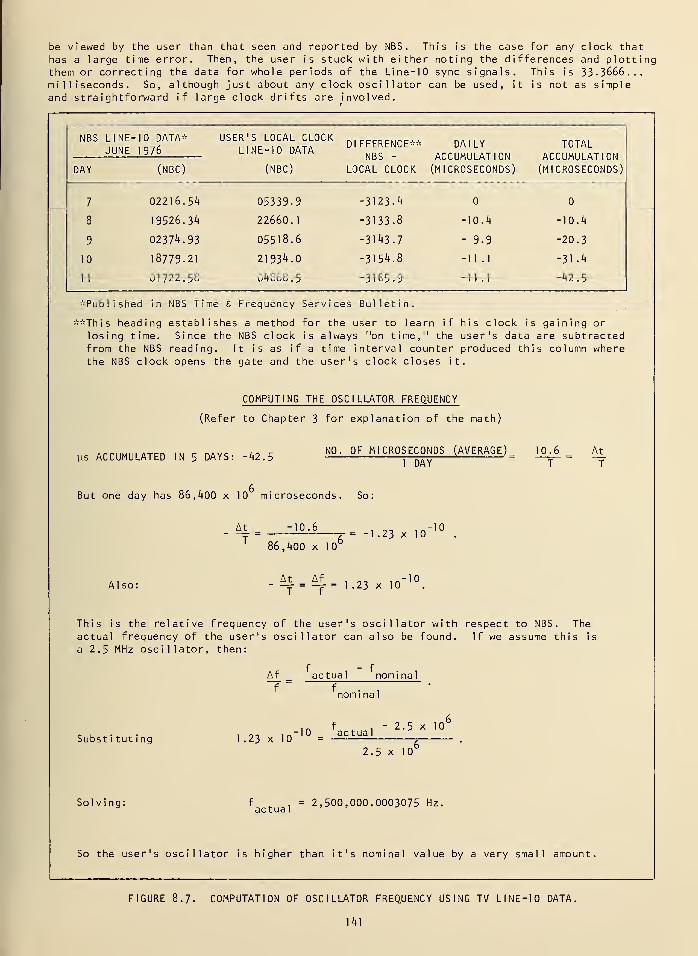
be viewed by the user than that seen and reported by NBS . This is the case for any clock thathas a large time error. Then, the user is stuck with either noting the differences and plottingthem or correcting the data for whole periods of the Line-10 sync signals. This is 33-3666...milliseconds. So, although just about any clock oscillator can be used, it is not as simpleand straightforward if large clock drifts are involved.
NBS LINE-10 DATA*JUNE 1976
USER'S LOCAL CLOCKLINE-10 DATA
DIFFERENCE**NBS -
LOCAL CLOCK
DAILYACCUMULATION(MICROSECONDS)
TOTALACCUMULATION(MICROSECONDS)DAY (NBC) (NBC)
7 02216. 54 05339.9 -3123.4
8 19526. 3^ 22660.1 -3133.8 -10.4 -10.4
9 02374.93 05518.6 -3143.7 - 9.9 -20.3
10 18779.21 21934.0 -3154.8 -11 .1 -31.4
11 01722.58 04888.5 -3165.9 -11 .1 -42.5
*Published in NBS Time & Frequency Services Bulletin.
-*This heading establishes a method for the user to learn if his clock is gaining or
losing time. Since the NBS clock is always "on time," the user's data are subtractedfrom the NBS reading. It is as if a time interval counter produced this column wherethe NBS clock opens the gate and the user's clock closes it.
COMPUTING THE OSCILLATOR FREQUENCY
(Refer to Chapter 3 for explanation of the math)
ys ACCUMULATED IN 5 DAYS: -42.5NO. OF MICROSECONDS (AVERAGE )
1 DAY
10.6 At
T
But one day has 86,400 x 10 microseconds. So:
At.
T
•10.6
86,400 x ]0
= -1 .23 x 10-10
Also:At Af ._ -10-= = —
j = 1 .23 x 10
This is the relative frequency of the user's oscillator with respect to NBS. The
actual frequency of the user's oscillator can also be found. If we assume this is
a 2.5 MHz oscillator, then:
Subst i tut ing
Solving:
Aff
.23 x 10
actual nominalr
• 1nomi nal
.. f . . - 2.5 x 10v
-10 actual
2.5 x 10
f ,= 2,500,000.0003075 Hz.
actual
So the user's oscillator is higher than it's nominal value by a very small amount
FIGURE 8.7. COMPUTATION OF OSCILLATOR FREQUENCY USING TV LINE-10 DATA.
141
8.6 GETTING TIME OF DAY FROM LINE-1
Since the Line-10 data are directly traceable to NBS , it contains time-of-day information.As noted in the above paragraph, it is ambiguous to 33 milliseconds. This means that if youwant to set a clock accurately (to within microseconds), you must first set it to within 33
milliseconds using some other scheme. A good way would be to use radio station WWV and an
oscilloscope. Once you are within the ambiguity range of the Line-10 data, you can use Line-10to set the clock more precisely. You would need to know the path and equipment delays. Thepath delay would just about have to be measured by carrying a clock to the NBS in Boulder.Once the delays are known, and if the user records data regularly from several networks, chancesare he can keep time to within several microseconds using Line-10.
The need to calibrate the path and resolve the ambiguity may seem to penalize this systemand suggest to the user that he use some other method, but there are not very many ways to get
accurate timing. Chapter 9 describes Loran-C techniques for accurate time setting. It, too,
needs to be calibrated and is ambiguous in the same way. So the steps are the same and Line-10
costs less.
8.7 MEASUREMENTS COMPARED TO THE USNO
The USNO also publishes Line-10 measurements on the East Coast TV networks originating in
New York City. Their measurements are made at the same time as the NBS measurements. Users
desiring to compare their clocks with the USNO may obtain the USNO data from their Time Services
Bulletin, Series k. For more information, write to the Time Services Division, U. S. Naval
Observatory, Washington, D. C. 20390.
8.8 LINE-10 EQUIPMENT AVAILABILITY
There are several manufacturers of TV Line-10 equipment. The NBS has also designed equip-
ment to recover the Line-10 pulse from a commercial TV receiver. The circuit diagram is shown
in figure 8.8. The instrument accepts 0.5 to 1.5 volts of video signal of either polarity from
a TV receiver and makes available a Line-10 pulse referenced to either the leading or trailingedge of sync. (Note that the Line-10 measurements published in the NBS Time and FrequencyServices- Bui let in are referenced to the trailing edge of the Line-10 sync pulse.) The problemis that you will have an error equal to the width of the sync pulse if you use the leading edgeand NBS uses the trailing edge. This design uses standard TTL integrated circuits and could be
assembled by a skilled technician.
For more information about equipment availability or the NBS-designed circuits, write to
the Time and Frequency Services Section, National Bureau of Standards, Boulder, CO 80302.
]h2
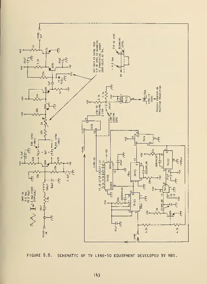
FIGURE 3.8. SCHEMATIC OF TV LINE-10 EQUIPMENT DEVELOPED BY NBS.
143
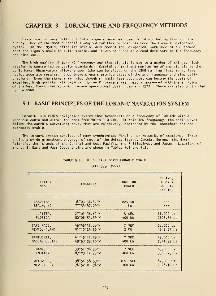
CHAPTER 9. LORAN-C TIME AND FREQUENCY METHODS
Historically, many different radio signals have been used for distributing time and fre-
quency. One of the most successful adapted for this purpose has been the Loran-C navigationsystem. In the 1950's, after its initial development for navigation, work done at NBS showedthat the signals could be quite stable, and it was proposed as a candidate service for frequencyand time use.
The high quality of Loran-C frequency and time signals is due to a number of things. Each
station is controlled by cesium standards. Careful control and monitoring of the signals by the
U. S. Naval Observatory allows a user (who can be placed on the USNO mailing list) to achieverapid, accurate results. Groundwave signals provide state of the art frequency and time cali-brations. Even the skywave signals, though slightly less accurate, can become the basis of
excellent high-quality calibrations. Loran-C coverage was greatly increased with the additionof the West Coast chains, which became operational during January 1977. These are also controlledby the USNO.
9. 1 BASIC PRINCIPLES OF THE LORAN-C NAVIGATION SYSTEM
Loran-C is a radio navigation system that broadcasts on a frequency of 100 kHz with a
spectrum contained within the band from 90 to 110 kHz. At this low frequency, the radio wavesfollow the earth's curvature; thus, they are relatively unbothered by the ionosphere and areextremely stable.
The Loran-C system consists of many synchronized "chains" or networks of stations. Thesechains provide groundwave coverage of most of the United States, Canada, Europe, the NorthAtlantic, the islands of the Central and West Pacific, the Philippines, and Japan. Locations of
the U. S. East and West Coast chains are shown in Tables 9-1 and 9.2.
TABLE 9.1- U. S. EAST COAST LORAN-C CHAIN
RATE 9930 (SS7)
STATIONNAME
LOCATIONFUNCTION,
POWER
CODING,DELAY &
BASELINELENGTH
CAROLINABEACH, NC
3V03'36.50"N77 5V»7.29"W
MASTER1 MW
JUPITER,FLORIDA
27°01'58.85"N
80°06'53.59"WW SEC400 kW
11 ,000 ys
2605-51 ys
CAPE RACE,NEWFOUNDLAND
46°46'31.88"N
53o 10'29.l6"W
X SEC
2 MW28,000 ys
8389-57 ys
NANTUCKET,MASSACHUSETTS
4l°15'12.29"N69
o 58'39.10"WY SEC
400 kW49,000 ys
3541.33 ys
DANA,
INDIANA
39°51 '08.30"N87°29'12.75"W
Z SEC
400 kW65,000 ys
3560.73 ys
WILDW00D,NEW JERSEY
38°56'58.59"N74°52'01 .9V'W
TEST SEC.
400 kW82,000 ys
2026.19 ys
145
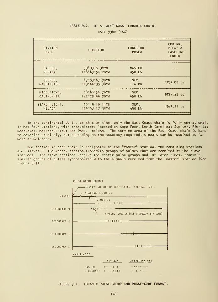
TABLE 9.2. U. S. WEST COAST LORAN-C CHAIN
RATE 99^0 (SS6)
STATIONNAME
LOCATIONFUNCTION,
POWER
CODING,DELAY &
BASELINELENGTH
FALLON,NEVADA
39°33'6.38"N118°49'56.20"W
MASTER450 kw
---
GEORGE,WASHINGTON
47°03'47.90"NI19°44'39.38"W
SEC.
1.4 MW2797.00 us
MIDDLETOWN,CALIFORNIA
38°46'56.76"NI22°29'44.30"W
SEC.
450 kw1094.52 ys
SEARCH LIGHT,
NEVADA35°19' I8.11"N
1 1 4°i*8 '
1 7- 35"WSEC.
450 kW1967.21 ys
In the continental U. S., at this writing, only the East Coast chain is fully operational,
It has four stations, with transmitters located at Cape Fear, North Carolina; Jupiter, Florida
Nantucket, Massachusetts; and Dana, Indiana. The service area of the East Coast chain is hard
to describe precisely, but depending on the accuracy required, signals can be received as far
west as Colorado.
One station in each chain is designated as the "master" station; the remaining stations
are "slaves." The master station transmits groups of pulses that are received by the slave
stations. The slave stations receive the master pulse groups and, at later times, transmit
similar groups of pulses synchronized with the signals received from the "master" station (See
figure 9.1).
PULSE GROUP FORMAT
MASTER
SECONDARY W
SECONDARY X
SECONDARY Y
SECONDARY Z
-START OF GROUP REPETITION INTERVAL (GRI)
f4-(-
SPACING 1 ,000 us
I I i n I I I . 1
2,000 us
1 GRI-
SPACING 1,000 us (ALL SECONDARY STATIONS)
I H I II I I
I I I I I I II
II II I I I I
PHASE CODE
1ST GRI
MASTER ++ +—
t
SECONDARY -I- ++-M
ALTERNATE GRI
FIGURE 9.1. LORAN-C PULSE GROUP AND PHASE-CODE FORMAT,
146
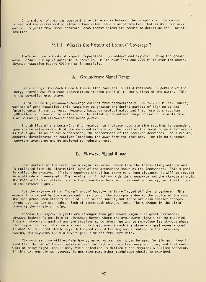
On a ship or plane, the constant time differences between the reception of the masterpulses and the corresponding slave pulses establish a 1 ine-of-pos i t ion that is used for navi-
gation. Signals from three separate Loran transmissions are needed to determine the line-of-
posi tion.
9. 1 . 1 What is the Extent of Loran-C Coverage ?
There are two methods of signal propagation: groundwave and skywave. Using the ground-wave, Loran-C timing is possible to about 1500 miles over land and 2000 miles over the ocean.
Skywave reception beyond 5000 miles is possible.
A. Groundwave Signal Range
Radio energy from each Loran-C transmitter radiates in all directions. A portion of the
energy travels out from each transmitting station parallel to the surface of the earth. This
is the so-called groundwave.
Useful Loran-C groundwave coverage extends from approximately 1500 to 2000 miles. Duringperiods of good reception, this range may be greater and during periods of high noise and
interference, it may be less. However, based on typical noise and interference situations,1500 miles is a reasonable estimate of the reliable groundwave range of Loran-C signals from a
station having 300 kilowatts peak pulse power.
The ability of the Loran-C timing receiver to indicate accurate time readings is dependentupon the relative strength of the received signals and the level of the local noise interference.As the signal-to-noise ratio decreases, the performance of the receiver decreases. As a result,accuracy deteriorates at receiver locations far away from the stations. For timing purposes,long-term averaging may be employed to reduce errors.
B. Skywave Signal Range
Some portion of the Loran radio signal radiates upward from the transmitting antenna andis reflected from the electrified layer of the atmosphere known as the ionosphere. This signalis called the skywave. If the groundwave signal has traveled a long distance, it will be reducedin amplitude and weakened. The receiver will pick up both the groundwave and the skywave signals,The receiver cannot easily lock to the groundwave because it is weak and noisy, so it will lockto the skywave signal.
But the skywave signal "moves" around because it is reflected off the ionosphere. Thismovement is caused by the corresponding motion of the ionosphere due to the action of the sun.
The most pronounced effects occur at sunrise and sunset, but there are also smaller changesthroughout the day and night. Each of these path changes looks like a change in the signalphase at the receiving point.
Because the skywave signals are stronger than groundwave signals at great distances,skywave lock-on is possible at distances beyond where the groundwave signals can be received.A strong skywave signal allows the receiver to do averaging and to reproduce its skywave phaseplot day after day. What we are saying is that, even though the skywave signal moves around,it does so in a predictable way. With good record-keeping and attention to the receivingsystem, the skywaves can yield very good time and frequency data.
The next section will explain how Loran works and how it can be used for timing. Keep in
mind that the use of Loran implies a need for high accuracy frequency and time, and that underweak or noisy signal conditions, cycle selection is difficult and requires a skilled operator.If this extreme timing accuracy is not required, other techniques should be examined.
147
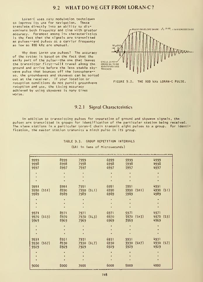
9.2 WHAT DO WE GET FROM LORAN-C ?
Loran-C uses many modulation techniquesto improve its use for navigation. Thesetranslate directly into an ability to dis-seminate both frequency and time with greateraccuracy. Foremost among its characteristicsis the fact that the signals are transmittedas pulses--and pulses at a carrier frequencyas low as 100 kHz are unusual.
Why does Loran use pulses? The accuracyof the system is based on the fact that the
early part of the pulse--the one that leaves
the transmitter first—will travel along the
ground and arrive before the less stable sky-wave pulse that bounces off the ionosphere--so, the groundwaves and skywaves can be sortedout at the receiver. If your location or
reception conditions do not permit groundwavereception and use, the timing accuracyachieved by using skywaves is many times
worse.
• PULSE ENVELOPE SHAPE = t2e
z,/65; t IN MICROSECONDS
r'
CYCLE ZEROCROSSING TO BEIDENTIFIED ANDTRACKED
FIGURE 9.2. THE 100 kHz LORAN-C PULSE
9.2.1 Signal Characteristics
In addition to transmitting pulses for separation of ground and skywave signals, the
pulses are transmitted in groups for identification of the particular station being received.The slave stations in a particular Loran-C chain transmit eight pulses to a group. For identi
fication, the master station transmits a ninth pulse in its group.
TABLE 9-3. GROUP REPETITION INTERVALS
(GRI In Tens of Microseconds)
99999998
9997
89998998
8997
79997998
7997
699969986997
•
59995998
5997
•
*»999
4998
4997
•
9991
99909989
(SSI)
•
8991
89908989
•
7991
79907989
*
(SL1)
•
6991
6990
6989
•
•
5991
5990
5989
•
(SHI)
•
^991
4990
4989
(si)
9971
99709969
(SS3)
•
8971
89708969
•
•
7971
79707969
(SL3)
•
6971
69706969
•
•
5971
5970
5969
•
(SH3)
•
4971
^970^969
•
(S3)
9931
99309929
(SS7)
8931
89308929
7931
79307929
(SL7)
6931
69306929
5931
59305929
(SH7)
*»931
^9304929
(S7)
9000 8000 7000 6000 5000 *»000
148
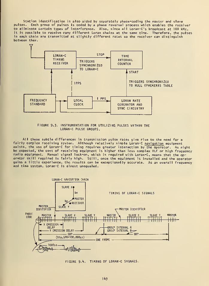
Station identification is also aided by separately phase-coding the master and slavepulses. Each group of pulses is coded by a phase reversal process which enables the receiverto eliminate certain types of interference. Also, since all Loran-C's broadcast at 100 kHz,it is possible to receive many different Loran chains at the same time. Therefore, the pulsesin each chain are transmitted at slightly different rates so the receiver can distinguishbetween them.
V
LORAN-CTIMINGRECEIVER
STOP
TRIGGERSSYNCHRONIZEDTO LORAN-C
TIMEINTERVALCOUNTER
1PPS
FREQUENCYSTANDARD
LOCALCLOCK
PPS
i L START
TRIGGERS SYNCHRONIZEDTO NULL EPHEMERIS TABLE
LORAN RATEGENERATOR ANDSYNC CIRCUITRY
FIGURE 9.3. INSTRUMENTATION FOR UTILIZING PULSES WITHIN THELORAN-C PULSE GROUPS.
All these subtle differences in transmission pulse rates give rise to the need for afairly complex receiving system. Although relatively simple Loran-C navigation equipmentexists, the use of Loran-C for timing requires greater interaction by the operator. As mightbe expected, the cost of receiving equipment is higher than less complex VLF or high frequencyradio equipment. Manual signal lock-on, which is required with Loran-C, means that the op-erator skill required is fairly high. Still, once the equipment is installed and the operatorgains a little experience, the results can be exceptionally accurate. As an overall frequencyand time system, Loran-C is almost unequaled.
LGRAN-C NAVIGATION CHAIN
SLAVE X»
PHASECODE
by.
SLAVE Y
bx
MASTER
• RECEIVER
SLAVE X SLAVE Ymm
TIMING OF LORAN-C SIGNALS
MASTER IDENTIFIER
. . - MASTER V SLAVE X SLAVE Y MASTER
mim trnlrni —1
-* X EMISSIONDELAY
h* Y EMISSION DELAY »-
GRP
(SS<J>,GPR=l00,000ys)
lOOOpS
-^%ma^—^Wlrtl/Mh
ZJ2-GROUP INTERVAL A
GROUP INTERVAL B-
ONE FRAME
FIGURE S.k. TIMING OF LORAN-C SIGNALS.
149
Figure 3.k shows how signals from a Loran-C chain are timed. Plus and minus signs overindividual pulses indicate the phase code, where (+) represents a relative phase of 0° and (-)
represents 180°. All master stations are phase-coded one way, and all slaves are phase-codedanother.
9.2.2 Time Setting
To make time calibrations, the user of Loran-C must take into account the fact that the
pulse repetition rates used are not at one pulse per second, nor are they at a convenientmultiple thereof. Instead, a time of coincidence, TOC (when a Loran pulse coincides with a
one-second pulse) may occur as infrequently as every sixteen minutes. After the receiver is
locked to the incoming signal, the one pul se-per-second timing output must be synchronized to
the time of coincidence. This is done by pushing a button on the receiver just before thecorrect second arrives. Assuming power is not lost, and the receiver does not lose lock, thetiming pulses will stay "on time." It is important to keep a battery supply connected to thereceiver to prevent loss of synchronization in case of power outages.
Loran-C is most often used when the required timing accuracies are equal to or better than
ten microseconds. Remember that any user of a timing system that provides accuracies of this
order must take into account path and equipment delays. In addition, he must pay very closeattention to how the receiving equipment is maintained and have the necessary battery backups.Simply stated, as with any scheme for time and frequency calibrations, if you are looking for
high accuracies, you must be willing to pay the price in equipment complexity and operatorattention.
The most difficult part of Loran-C timing is recognizing the sample point where thereceiver is locked onto the signal. Since Loran-C operates at 100 kHz, it is possible to lock
onto carrier zero crossings separated by the 10 microsecond period. An oscilloscope display ofLoran-C pulses is imperative and under noisy conditions, it is of great assistance to the
operator to have a plot made of the received pulse showing the exact position of the samplepoint. Receiving equipment sold for Loran timing usually incorporates this plotting capability.
Setting Local Time . In a timing system, it is often convenient or necessary to operate"on time" rather than simply with a known but possibly larger time offset. The equipmentneeded is basically a clock that employs a display for the time-of-day readout. The onlyaspect of the system that may be unconventional enough to require explanation is the digitalslewing system used to shift timing outputs forward or backward in time. Basically, this is a
digital phase shifter.
Normally, the phase shifter input and output are at 1 MHz. When the shifter receives a
step-command pulse, the phase of the output advances or drops back by exactly one microsecond.Thus, if "N" step-command pulses are fed into the phase shifter, the output (and all subsequentdivider outputs) will shift by exactly "N" microseconds.
The following steps show how to synchronize local time by Loran-C:
1. Synchronize the clock time to coarse UTC by reference to WWV . Allow for propagationdelay (1 microsecond per 1 86 miles) and receiver delay.
2. Acquire and track on desired cycles of Loran-C transmission from either a slave or
the master transmitter.
3. Synchronize clock phase to Loran receiver tracking gate (tracking gate is locked to
received Loran-C signal).
k. Using Loran-C emission and propagation delay figures furnished by USNO and receiver
delay from the receiver operating manual, the clock can be set "on time" with the
beginning of the transmitted pulse.
5. On an upcoming t ime-of-coincidence (TOC) , operate the clock-sync controls so that
clock circuits will synchronize to the internal "on time" signal when the TOC appears.
50
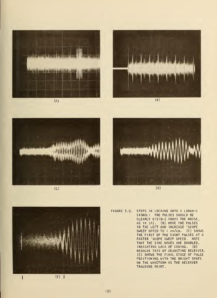
1 I1W!
i.iilri
(A)
FIGURE 9.5- STEPS IN LOCKING ONTO A LORAN-CSIGNAL: THE PULSES SHOULD BE
CLEARLY VISIBLE ABOVE THE NOISE,AS IN (A). (B) MOVE THE PULSESTO THE LEFT AND INCREASE 'SCOPE
SWEEP SPEED TO 1 ms/cm. (C) SHOWSTHE FIRST OF THE EIGHT PULSES AT A
FASTER 'SCOPE SWEEP SPEED. NOTE
THAT THE SINE WAVES ARE DOUBLED,INDICATING LACK OF CODING. (D)
RESOLVE THIS BY ADJUSTING RECEIVER.
(E) SHOWS THE FINAL STAGE OF PULSEPOSITIONING WITH THE BRIGHT SPOTSON THE WAVEFORM AS THE RECEIVERTRACKING POINT.
151
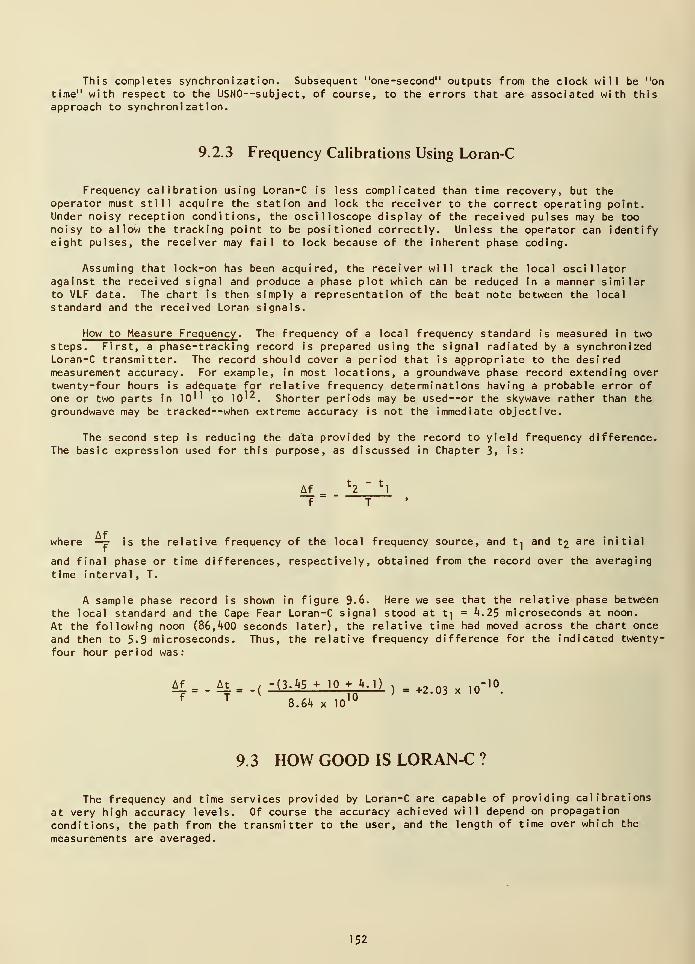
This completes synchronization. Subsequent "one-second" outputs from the clock will be "on
time" with respect to the USNO
—
subject, of course, to the errors that are associated with thisapproach to synchronization.
9.2.3 Frequency Calibrations Using Loran-C
Frequency calibration using Loran-C is less complicated than time recovery, but theoperator must still acquire the station and lock the receiver to the correct operating point.Under noisy reception conditions, the oscilloscope display of the received pulses may be toonoisy to allow the tracking point to be positioned correctly. Unless the operator can identifyeight pulses, the receiver may fail to lock because of the inherent phase coding.
Assuming that lock-on has been acquired, the receiver will track the local oscillatoragainst the received signal and produce a phase plot which can be reduced in a manner similarto VLF data. The chart is then simply a representation of the beat note between the local
standard and the received Loran signals.
How to Measure Frequency . The frequency of a local frequency standard is measured in twosteps. First, a phase-tracking record is prepared using the signal radiated by a synchronizedLoran-C transmitter. The record should cover a period that is appropriate to the desiredmeasurement accuracy. For example, in most locations, a groundwave phase record extending overtwenty-four hours is adequate for relative frequency determinations having a probable error ofone or two parts in 10'' to lO'^. Shorter periods may be used—or the skywave rather than the
groundwave may be tracked—when extreme accuracy is not the immediate objective.
The second step is reducing the data provided by the record to yield frequency difference.The basic expression used for this purpose, as discussed in Chapter 3, is:
Af h ~ ll
f T
where —r is the relative frequency of the local frequency source, and tj and t2 are initial
and final phase or time differences, respectively, obtained from the record over the averaging
time interval , T.
A sample phase record is shown in figure S.G. Here we see that the relative phase between
the local standard and the Cape Fear Loran-C signal stood at t] = 4.25 microseconds at noon.
At the following noon (86,400 seconds later), the relative time had moved across the chart once
and then to 5.9 microseconds. Thus, the relative frequency difference for the indicated twenty-
four hour period was:
Af = . At m _(-J3A5+ 1Q + 1.1)
, = +2 . 03 x 10-
f T8.64 x 10
10
10
9.3 HOW GOOD IS LORAN-C ?
The frequency and time services provided by Loran-C are capable of providing calibrations
at very high accuracy levels. Of course the accuracy achieved will depend on propagation
conditions, the path from the transmitter to the user, and the length of time over which the
measurements are averaged.
152
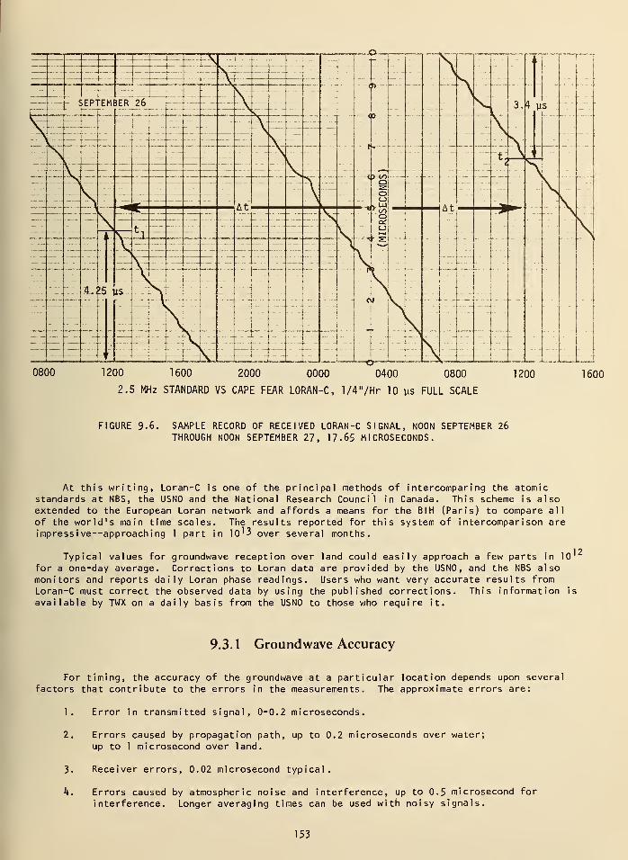
1
—
zz
_z
.
—
j
<
a.
i>—
"
—
— -ZZ zz
~
—
-
1 r~~
"--
— — — ....
—"—
3.
———— -— ————— -V"
—.
—
~- ::
ZZ CCI ! HI :• "j£. —<
t
4 us
<
, . ...
.
-—— — —:—
~t;1
-
—
-— — ——•— — — — v~ —
•
V
\
zz-- — N5Z
._. —--
— — -"- 9':- zz— -
. . .
ZZ
— V— - —— - o "—
1
—ej
.„—, _™.. ^ „— At V UI At
:z zz— — —
i
ZZ >
.:..:
c
-—
c
.;„.. zz
_
* .
—
k_ -
r s:iz-
-——
—
— ; i s
—
- - - •
>
—
'
zz
—.. ._,..
_4z is is
zz \
—
-
-
V-
z z ....
zz
z:zz—:z:^ "Z"—
—_Lj
0800 1200 1600 2000 0000 0400 0800
2.5 MHz STANDARD VS CAPE FEAR LORAN-C, 1/4 "/Hr 10 ys FULL SCALE
1200 1600
FIGURE 9.6. SAMPLE RECORD OF RECEIVED LORAN-C SIGNAL, NOON SEPTEMBER 26
THROUGH NOON SEPTEMBER 27, 17-65 MICROSECONDS.
At this writing, Loran-C is one of the principal methods of intercompar ing the atomicstandards at NBS, the USN0 and the National Research Council in Canada. This scheme is alsoextended to the European Loran network and affords a means for the BIH (Paris) to compare all
of the world's main time scales. The results reported for this system of intercompar i son areimpressive—approaching 1 part in 10^3 over several months.
Typical values for groundwave reception over land could easily approach a few parts in 10
for a one-day average. Corrections to Loran data are provided by the USN0, and the NBS alsomonitors and reports daily Loran phase readings. Users who want very accurate results fromLoran-C must correct the observed data by using the published corrections. This information is
available by TWX on a daily basis from the USN0 to those who require it.
12
9.3.1 Groundwave Accuracy
For timing, the accuracy of the groundwave at a particular location depends upon several
factors that contribute to the errors in the measurements. The approximate errors are:
1. Error in transmitted signal, 0-0.2 microseconds.
2. Errors caused by propagation path, up to 0.2 microseconds over water;
up to 1 microsecond over land.
3. Receiver errors, 0.02 microsecond typical.
k. Errors caused by atmospheric noise and interference, up to 0.5 microsecond for
interference. Longer averaging times can be used with noisy signals.
153
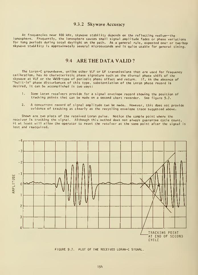
9.3.2 Skywave Accuracy
At frequencies near 100 kHz, skywave stability depends on the reflecting medium--theionosphere. Frequently, the ionosphere causes small signal amplitude fades or phase variationsfor long periods during total daylight on the path. As a general rule, expected one- or two-hopskywave stability is approximately several microseconds and is quite usable for general timing.
9.4 ARE THE DATA VALID ?
The Loran-C groundwave, unlike other VLF or LF transmissions that are used for frequencycalibration, has no characteristic phase signature such as the diurnal phase shift of theskywave at VLF or the WWVB-type of periodic phase offset and return. If, in the absence of"built-in" phase disturbances of this type, substantiation of the Loran phase record isdesired, it can be accomplished in two ways:
1. Some Loran receivers provide for a signal envelope record showing the position oftracking points that can be made on a second chart recorder. See figure 9.7.
2. A concurrent record of signal amplitude can be made. However, this does not provideevidence of tracking as clearly as the recycling envelope trace suggested above.
Shown are two plots of the received Loran pulse. Notice the sample point where thereceiver is tracking the signal. Although this method does not always guarantee cycle count,it at least will allow the operator to reset the receiver at the same point after the signal is
lost and reacquired.
Q=5
~
TRACKING POINTAT END OF SECONDCYCLE
FIGURE 9-7. PLOT OF THE RECEIVED LORAN-C SIGNAL.
15**
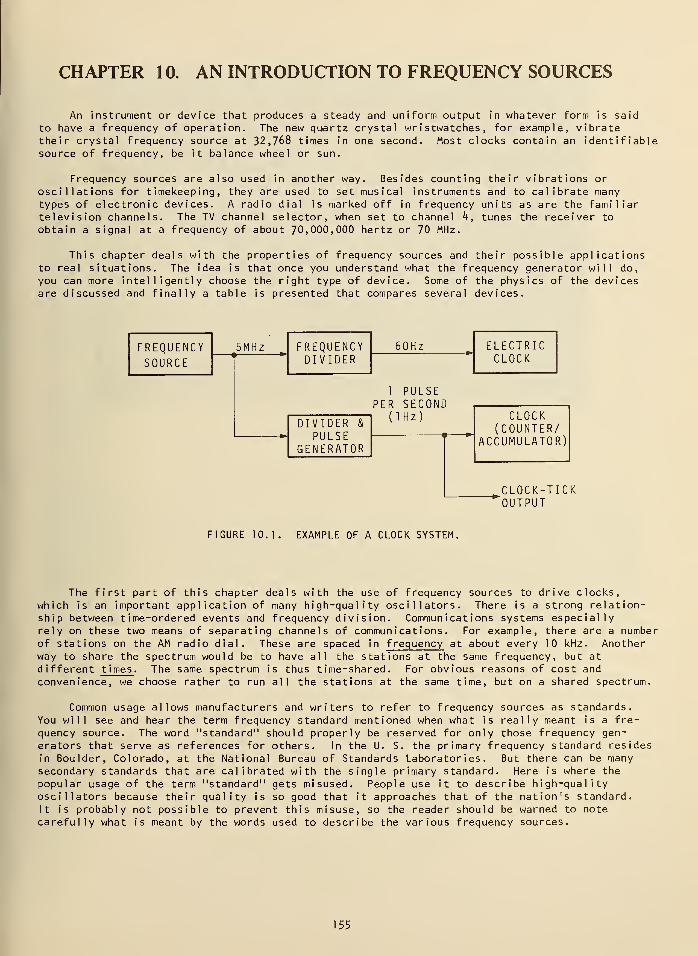
CHAPTER 10. AN INTRODUCTION TO FREQUENCY SOURCES
An instrument or device that produces a steady and uniform output in whatever form is said
to have a frequency of operation. The new quartz crystal wr i stwatches , for example, vibratetheir crystal frequency source at 32,768 times in one second. Most clocks contain an identifiablesource of frequency, be it balance wheel or sun.
Frequency sources are also used in another way. Besides counting their vibrations or
oscillations for timekeeping, they are used to set musical instruments and to calibrate manytypes of electronic devices. A radio dial is marked off in frequency units as are the familiartelevision channels. The TV channel selector, when set to channel *t, tunes the receiver to
obtain a signal at a frequency of about 70,000,000 hertz or 70 MHz.
This chapter deals with the properties of frequency sources and their possible applicationsto real situations. The idea is that once you understand what the frequency generator will do,
you can more intelligently choose the right type of device. Some of the physics of the devicesare discussed and finally a table is presented that compares several devices.
FREQUENCYSOURCE
5MHz FREQUENCYDIVIDER
DIVIDER &
PULSEGENERATOR
60Hz
1 PULSEPER SECOND
(1Hz)
ELECTRICCLOCK
CLOCK(COUNTER/
ACCUMULATOR
CLOCK-TICK'OUTPUT
FIGURE 10.1. EXAMPLE OF A CLOCK SYSTEM.
The first part of this chapter deals with the use of frequency sources to drive clocks,which is an important application of many high-quality oscillators. There is a strong relation-ship between time-ordered events and frequency division. Communications systems especiallyrely on these two means of separating channels of communications. For example, there are a numberof stations on the AM radio dial. These are spaced in frequency at about every 10 kHz. Anotherway to share the spectrum would be to have all the stations at the same frequency, but at
different times . The same spectrum is thus time-shared. For obvious reasons of cost and
convenience, we choose rather to run all the stations at the same time, but on a shared spectrum.
Common usage allows manufacturers and writers to refer to frequency sources as standards.
You will see and hear the term frequency standard mentioned when what is really meant is a fre-
quency source. The word "standard" should properly be reserved for only those frequency gen-
erators that serve as references for others. In the U. S. the primary frequency standard resides
in Boulder, Colorado, at the National Bureau of Standards Laboratories. But there can be manysecondary standards that are calibrated with the single primary standard. Here is where the
popular usage of the term "standard" gets misused. People use it to describe high-qualityoscillators because their quality is so good that it approaches that of the nation's standard.
It is probably not possible to prevent this misuse, so the reader should be warned to notecarefully what is meant by the words used to describe the various frequency sources.
155
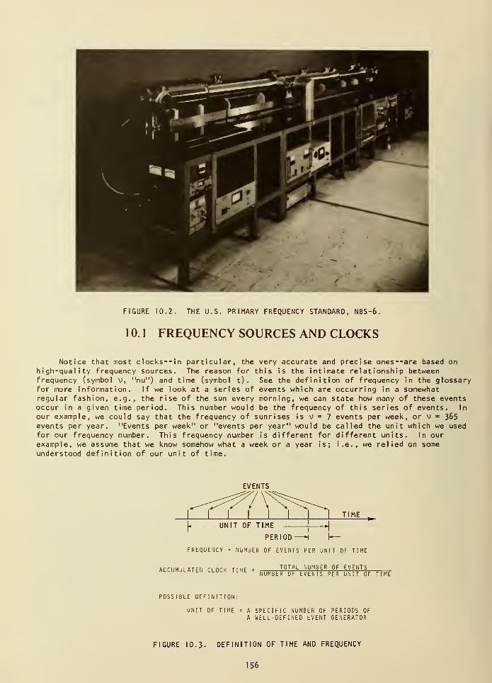
FIGURE 10.2. THE U.S. PRIMARY FREQUENCY STANDARD, NBS-6.
1 0. 1 FREQUENCY SOURCES AND CLOCKS
Notice that most clocks--in particular, the very accurate and precise ones--are based onhigh-quality frequency sources. The reason for this is the intimate relationship betweenfrequency (symbol v, "nu") and time (symbol t) . See the definition of frequency in the glossaryfor more information. If we look at a series of events which are occurring in a somewhatregular fashion, e.g., the rise of the sun every morning, we can state how many of these eventsoccur in a given time period. This number would be the frequency of this series of events. In
our example, we could say that the frequency of sunrises is v = 7 events per week, or v = 365events per year. "Events per week" or "events per year" would be called the unit which we used
for our frequency number. This frequency number is different for different units. In ourexample, we assume that we know somehow what a week or a year is; i.e., we relied on some
understood definition of our unit of time.
EVENTS
TIME
UNIT OF TIME
PERIOD —H h—FREQUENCY = NUMBER OF EVENTS PER UNIT OF TIME
ACCUMULATED CLOCK TIME TOTAL NUMBER OF EVENTSNUMBER OF EVENTS PER UNIT OF TIME
POSSIBLE DEFINITION:
UNIT OF TIME = A SPECIFIC NUMBER OF PERIODS OFA WELL-DEFINED EVENT GENERATOR
FIGURE 10.3. DEFINITION OF TIME AND FREQUENCY
156
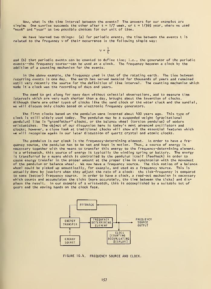
Now, what is the time interval between the events? The answers for our examples are
simple.: One sunrise succeeds the other after t = 1/7 week, or t = 1/3&5 year, where we used
"week" and "year" as two possible choices for our unit of time.
We have learned two things: (a) for periodic events, the time between the events t is
related to the frequency v of their occurrence in the following simple way:
1
v = -
and (b) that periodic events can be counted to define time; i.e., the generator of the periodicevents--the frequency source--can be used as a clock. The frequency becomes a clock by the
addition of a counting mechanism for the events.
In the above example, the frequency used is that of the rotating earth. The time betweenrecurring events is one day. The earth has served mankind for thousands of years and remaineduntil very recently the source for the definition of time interval. The counting mechanism whichmade it a clock was the recording of days and years.
The need to get along for many days without celestial observations, and to measure time
intervals which are very much shorter than a day, brought about the invention of clocks.Although there are other types of clocks like the sand clock or the water clock and the sundial,we will discuss only clocks based on electronic frequency generators.
The first clocks based on the pendulum were invented about 400 years ago. This type ofclock is still widely used today. The pendulum may be a suspended weight (gravitationalpendulum) like in "grandfather" clocks, or the balance wheel (torsion pendulum) of modernwr istwatches. The object of our discussion here is today's most advanced oscillators and
clocks; however, a close look at traditional clocks will show all the essential features whichwe will recognize again in our later discussion of quartz crystal and atomic clocks.
The pendulum in our clock is the frequency-determining element. In order to have a fre-quency source, the pendulum has to be set and kept in motion. Thus, a source of energy is
necessary together with the means to transfer this energy to the frequency-determining element.In a wristwatch, this source of energy is typically the winding spring or battery. The energyis transferred by a means which is controlled by the pendulum itself (feedback) in order to
cause energy transfer in the proper amount at the proper time in synchronism with the movementof the pendulum or balance wheel. We now have a frequency source. The tick motion of a balancewheel could be picked up acoustically, for example, and used as a frequency source. This is
actually done by jewelers when they adjust the rate of a clock: the tick-frequency is comparedto some (better) frequency source. In order to have a clock, a read-out mechanism is necessarywhich counts and accumulates the ticks (more accurately, the time between the ticks) and dis-
plays the result. In our example of a wristwatch, this is accomplished by a suitable set ofgears and the moving hands on the clock face.
ENERGYSOURCE
FEEDBACK
ENERGYTRANSFER
FREQUENCYDETERMINING
ELEMENT
FREQUENCYSOURCEOUTPUT
CLOCK(COUNTINGACCUMULATING
DISPLAY )
FIGURE 10.4. FREQUENCY SOURCE AND CLOCK.
157
We have just discussed how the addition of a mechanism to a frequency source which countsand accumulates and possibly displays the result creates a clock. This task can also be per-formed by an electronic frequency divider which, for example, derives a frequency of 60 Hz
directly from a 5 MHz crystal oscillator (fig. 10.1). The 60 Hz voltage can be used to drivean electrical clock motor similar to those driven by the 60 Hz power line frequency that we useat home and at work. Or, an additional electric pulse generator may be used that generates onevery sharp electrical pulse per second. The time interval of 1 second between the pulses(corresponding to a frequency of 1 Hz) is derived from the output of our frequency source. Thepulses can be directly used in time comparisons with those of other similar clocks, or theycan drive a counter/accumulator.
The electric power line is a very good frequency source for many applications. A clockdriven from the power line will keep excellent time. This is because the power system is care-fully controlled to maintain its frequency within definite limits. By increasing and decreasingthe individual generator frequencies, the flow of power in the interconnected system can be
regulated. Each power company is notified in advance to set their frequency to a particularvalue so that the millions of clocks on the system--those in homes and offices across the
country-will gain or lose time as required to keep the clocks correct. The time correctionsare usually done at night.
The basic unit of time is the second (symbol s). It is defined with reference to a
frequency-determining element. Since 1967, by international agreement, this element or "naturalpendulum" has been the cesium atom. One second is defined in the official wording as "theduration of 9,192,631,770 periods of the radiation corresponding to the transition between the
two hyperfine levels of the ground state of the cesium-133 atom." Accordingly, the frequencyof the cesium pendulum is 9,192,631,770 events per second (the cesium atom is a very rapidlyoscillating pendulum). The unit of frequency is then defined as hertz (symbol Hz) which meansthe repetitive occurrence of one event per second (the use of "hertz" is preferred to the olderterm "cycle per second", cps)
.
1 0. 2 THE PERFORMANCE OF FREQUENCY SOURCES
The performance of a frequency source is usually described in terms of its accuracy,reproducibility, and stability. These are defined as:
Accuracy: How well does it relate to the definition? In the case of
frequency, this means how well it relates to the definitionof a second (in terms of cesium) mentioned previously.
Reproducibility: If you built a number of such frequency sources and adjustedthem properly, how well would they agree in frequency?This term obviously applies to sources that are manufacturedand then tested to see how they differ.
Stability: Once the device is set to a given frequency, how well does
it generate that value during some period of time?
It is obvious from these definitions that frequency accuracy will be of great interest in
scientific measurements and in the evaluation and intercompar ison of the most advanced devices.
Good reproducibility is an asset in applications where it is important to expect some agreement
among several devices. However, the stability of a frequency source is usually most important
to the user.
The frequency stability (symbol o, "sigma") of a frequency source will depend on a variety
of internal and external physical and electronic influences that cause frequency fluctuations.
The frequency stability measured will be defined by the procedure used for the measurement. To
explain, frequency stability can be measured by taking a reasonably large number of successive
readings on an electronic counter which counts the frequency of the device to be evaluated.
Each counter reading (in hertz) is obtained by counting the output frequency for some specified
time (the sampling time "tau", symbol x) . This sampling time can usually be chosen by simply
adjusting a knob on the counter; for example, a sampling time of 0. 1 s or 1 s or 1 s may be
chosen. The result can be expected to change as x changes. So the stability needs to be
defined for a certain "tau".
158
Further, it might be expected that fluctuations in the readings of measured frequencywould tend to average out if observed long enough. This is not always so. The stability ofthe frequency source (sigma or a) will therefore usually depend on the sampling time of themeasurement and tends to get smaller with longer sampling times, T. But, again, there are manyexceptions to this.
It may happen that the frequency fluctuations at some later time are partially caused by,
or depend to some degree upon, the previous fluctuations. In this case, the computed value of awill depend on the particular way in which the many counter readings are averaged and evaluated.Another influence on measured stability depends on whether the counter starts counting againimmediately after completion of the preceeding count or if some time elapses ("dead-time")before counting starts again.
Finally, the electronic circuits used in measuring frequency stability will have a finiteresponse time; i.e., they cannot follow frequency fluctuations faster than some given rate.For example, our eyes cannot register light fluctuations which occur faster than about every1/10 of a second; using eq. (1), we say that the eye has a frequency response of 10 Hz, or thatits bandwidth is only 10 Hz; i.e., the eye cannot follow frequencies higher than 10 Hz.
In order to measure frequency stabilities for sampling times smaller than some value t,
our measurement equipment has to provide for an electronic frequency bandwidth which is largerthan 1/t.
To summarize: A recommended way of properly measuring and describing frequency stabilityis the following: (a) make sure that the frequency bandwidth of the total measuring setup is
larger than 1/t, where x is the smallest desired sampling time; (b) use a counter with a dead-time as small as possible (the dead-time should be less than the reciprocal bandwidth; if not,use the computation procedures that exist to allow for larger dead-times); (c) take a suffi-ciently large number of readings at a given sampling time which is held constant and compute:
7 Addition of the squares of the differences between successive readings2 x total number of differences used
(In the scientific literature this a is often called the square root of the Allan variance.)The counter readings can be taken in Hz; a will then have the dimensions of Hz; (d) repeatstep (c) for other sampling times x and tabulate or plot a as it depends on x.
Commonly, a will be expressed as a relative value. Existing literature often uses the
term "fractional" instead of relative, so the reader should treat the two terms equal ly--theymean the same thing. The value obtained for the frequency stability is divided by the carrierfrequency. For example, if a frequency stability of a§v = 10 Hz were measured at a carrierfrequency of v = 5 MHz (MHz = megahertz = million Hz) then the fractional or relative frequencystabi 1 i ty would be
a = a. , = 2 x 10y 6v/v
We denote the kind of a we are using by a subscript, 6v ("delta nu") , referring to fre-quency fluctuation (measured in Hz) or 6v/v = y, referring to relative frequency fluctuations(d imens ionless) . A stability of one part in a million is thus
a = 1 x 10" 6,
y
and one part in a trillion is written as
a = 1 x 10" 12.
y
There is a sound basis for using the relative frequency stability a instead of using
frequency stability a$v directly. o~y
is a numeric and is independent of the actual operatingfrequency of the oscillator being discussed. Thus, it is possible to compare the stability
of a 10 MHz oscillator with one that has an output at 10 kHz.
159
In fact, many high-quality oscillators have outputs at 1, 5, and 10 MHz. But an applica-tion for these sources might require the generation of a different frequency, e.g., the tele-vision color subcarrier signal at 3-58 MHz. If the original source, before the synthesis ofthe TV signal, had a relative frequency stability of one part per million (l x 10"°), then the3.58 MHz signal would have the same relative frequency stability a .
This assumes, of course, that the synthesis or generation of new frequencies does notchange the stability of the frequency source. This is generally true for most applications.
10.3 USING FREQUENCY STABILITY DATA
Suppose you have a clock. Let's say its frequency source is a crystal oscillator, and youwant to know the time error. If you know enough about the oscillator, you can compute the timeerror. You can even predict the error ahead of time— fairly accurately, too.
First, let's define a few things that we will need to write an equation. There are onlyabout three things that can happen to our clock—assuming we don't drop it or pull the plug!
1. The clock could be reading the wrong time because we didn't set it at all or becausewe set it wrong. Call this the initial time error AtQ . Until we correct it, we have
to have it in our equation as a constant.
2. The frequency of the oscillator driving the clock may be fluctuating. If that is the
case, then we will have a term in our equation that relates the fluctuation and the
length of time it has been drifting. Let's call this length of time t. It would be
the time from zero time (when the clock was right or we measured the error AtQ ) till
now. From what we said about the stability, we see that we need a term such as:
a (t) x t.
Actually, we know the value of t that we want. It's simply t, the time since we last
set the clock. So our term becomes approximately:
a (t = t) x t.
This then takes care of the instabilities of the oscillator frequency driving our
clock.
3. There is one more possible error. Was the oscillator "on frequency" when it started
to drift? If it was not, then we must account for this offset. To do this, we
define the relative frequency offset as:
Av .
This term means that our oscillator may have had a frequency error when it started to
drift. In other words, we allow for an arbitrary starting point.
To review then, we have an oscillator connected to a clock and it may or may not have
had a time error At in addition to having or not
either the correct or incorrect frequency Av/v x t
had a time error At in addition to having or not having some drift a x t from
Addition of these time errors gives us the clock error at time t.
At = At + a (x = t) x t + — x to y v
The equation shows how the relative frequency offset and stability accumulate time
error as t grows larger. Let's plug in some numbers and see what happens to our
clock. Assume the oscillator was off frequency by 1 part in 10' , fluctuates by
1 part in loll per day, and had a 1 microsecond error yesterday at this time.
Reading the graph we see that our clock error would be about three microseconds.
We get almost 1 microsecond error from fluctuations, 1 microsecond from frequency
offset and one from our initial setting error.
160
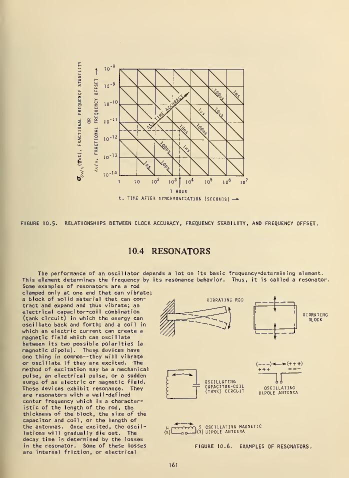
10
C/l (/)£ 10
:>
-9
-1 <* <* in" 1 1< o u. 10
- 10
10'
12
10"
x <£sV
\ cSi V\\^>y V \XX r^
\\1 10 10
2io
3
I10
410
510
610
7
1 HOUR
t, TIME AFTER SYNCHRONIZATION (SECONDS)—*
FIGURE 10.5- RELATIONSHIPS BETWEEN CLOCK ACCURACY, FREQUENCY STABILITY, AND FREQUENCY OFFSET.
10.4 RESONATORS
VIBRATING ROD
VIBRATINGBLOCK
The performance of an oscillator depends a lot on its basic frequency-determining element.
This element determines the frequency by its resonance behavior. Thus, it is called a resonator,
Some examples of resonators are a rod
clamped only at one end that can vibrate;a block of solid material that can con-tract and expand and thus vibrate; an
electrical capacitor-coil combination(tank circuit) in which the energy can
oscillate back and forth; and a coil in
which an electric current can create a
magnetic field which can oscillatebetween its two possible polarities (a
magnetic dipole). These devices have
one thing in common--they will vibrateor oscillate if they are excited. Themethod of excitation may be a mechanicalpulse, an electrical pulse, or a suddensurge of an electric or magnetic field.
These devices exhibit resonance. Theyare resonators with a well-definedcenter frequency which is a character-istic of the length of the rod, thethickness of the block, the size of the
capacitor and coil, or the length of
the antennas. Once excited, the oscil-lations will gradually die out. Thedecay time is determined by the lossesin the resonator. Some of these lossesare internal friction, or electrical
(+ + +)+ + +
OSCILLATINGCAPACITOR-COIL(TANK) CIRCUIT
IfOSCILLATING
DIPOLE ANTENNA
H ry~Y^r>rw~} S
(S)L_^>o—I(n
OSCILLATING MAGNETICDIPOLE ANTENNA
FIGURE 10.6. EXAMPLES OF RESONATORS
161
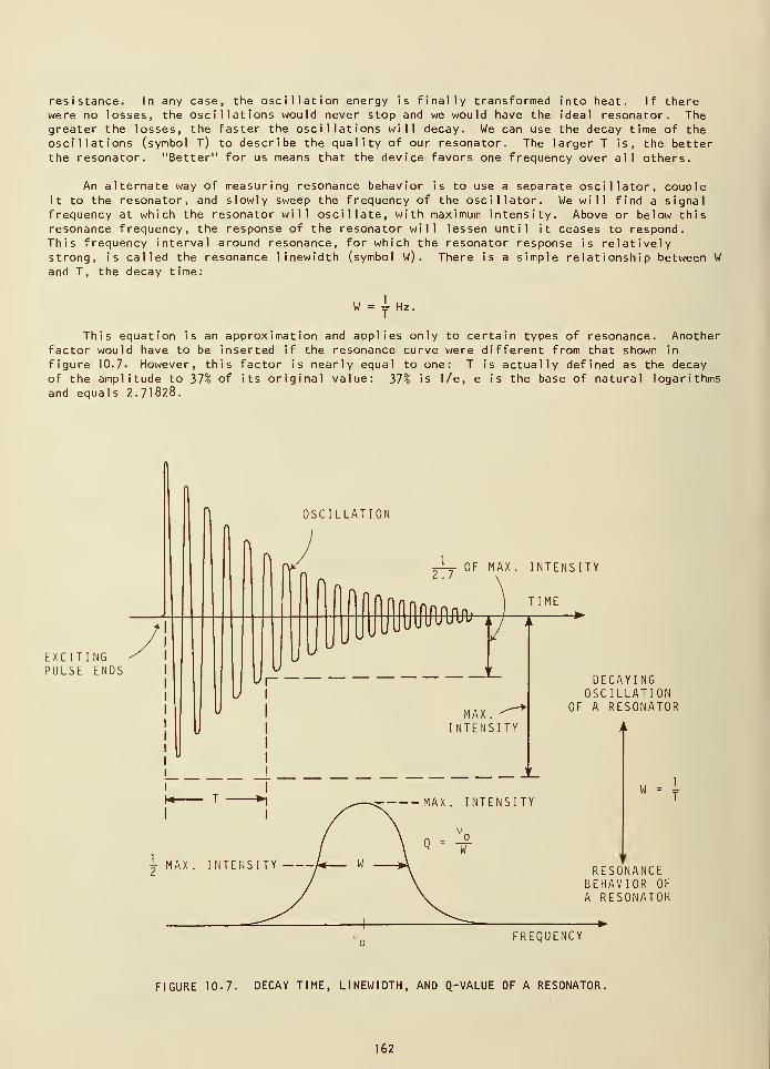
resistance. In any case, the oscillation energy is finally transformed into heat. If therewere no losses, the oscillations would never stop and we would have the ideal resonator. Thegreater the losses, the faster the oscillations will decay. We can use the decay time of theoscillations (symbol T) to describe the quality of our resonator. The larger T is, the better
the resonator. "Better" for us means that the device favors one frequency over all others.
An alternate way of measuring resonance behavior is to use a separate oscillator, coupleit to the resonator, and slowly sweep the frequency of the oscillator. We will find a signalfrequency at which the resonator will oscillate, with maximum intensity. Above or below thisresonance frequency, the response of the resonator will lessen until it ceases to respond.This frequency interval around resonance, for which the resonator response is relativelystrong, is called the resonance 1 inewidth (symbol W) . There is a simple relationship between Wand T, the decay time:
W = j Hz.
This equation is an approximation and applies only to certain types of resonance. Anotherfactor would have to be inserted if the resonance curve were different from that shown in
figure 10.7- However, this factor is nearly equal to one: T is actually defined as the decayof the amplitude to 37% of its original value: 37% is 1/e, e is the base of natural logarithmsand equals 2.71828.
OSCILLATION
OF MAX. INTENSITY
EXCITINGPULSE ENDS
DECAYINGOSCILLATION
OF A RESONATOR
W .T
RESONANCEBEHAVIOR OF
A RESONATOR
FREQUENCY
FIGURE 10-7. DECAY TIME, LINEWIDTH, AND Q-VALUE OF A RESONATOR.
162
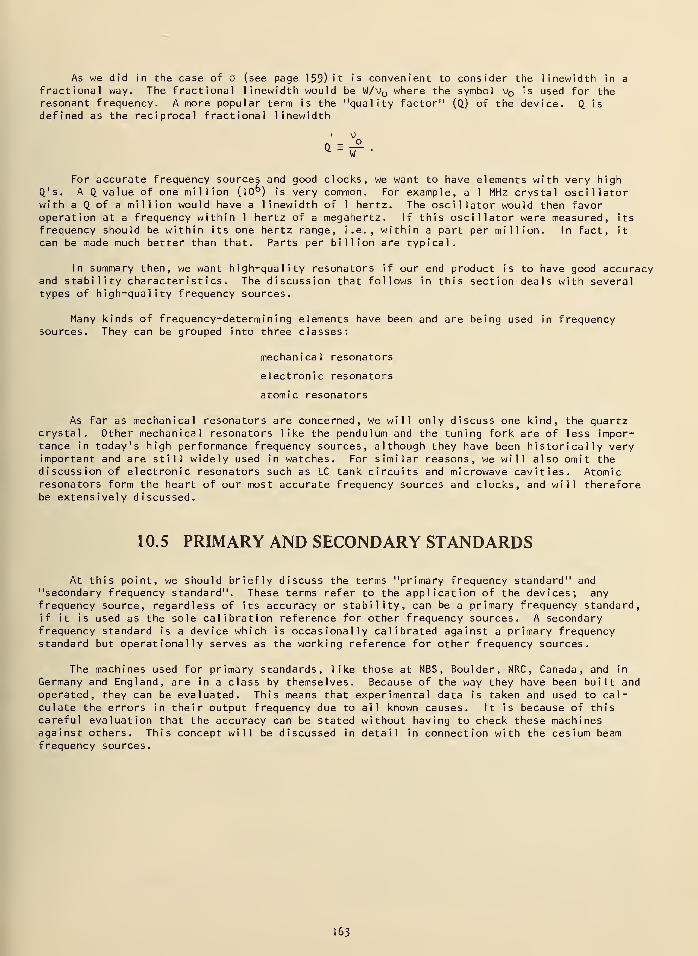
As we did in the case of a (see page 159) it is convenient to consider the linewidth in a
fractional way. The fractional linewidth would be W/v where the symbol v is used for theresonant frequency. A more popular term is the "quality factor" (Oj of the device. Q. is
defined as the reciprocal fractional linewidth
• v
For accurate frequency sources and good clocks, we want to have elements with very highQ's. A Q. value of one million (10°) is very common. For example, a 1 MHz crystal oscillatorwith a Q of a million would have a linewidth of 1 hertz. The oscillator would then favoroperation at a frequency within 1 hertz of a megahertz. If this oscillator were measured, its
frequency should be within its one hertz range, i.e., within a part per million. In fact, it
can be made much better than that. Parts per billion are typical.
In summary then, we want high-quality resonators if our end product is to have good accuracyand stability characteristics. The discussion that follows in this section deals with severaltypes of high-quality frequency sources.
Many kinds of frequency-determining elements have been and are being used in frequencysources. They can be grouped into three classes:
mechanical resonators
electronic resonators
atomic resonators
As far as mechanical resonators are concerned, we will only discuss one kind, the quartzcrystal. Other mechanical resonators like the pendulum and the tuning fork are of less impor-tance in today's high performance frequency sources, although they have been historically veryimportant and are still widely used in watches. For similar reasons, we will also omit thediscussion of electronic resonators such as LC tank circuits and microwave cavities. Atomicresonators form the heart of our most accurate frequency sources and clocks, and will thereforebe extensively discussed.
10.5 PRIMARY AND SECONDARY STANDARDS
At this point, we should briefly discuss the terms "primary frequency standard" and"secondary frequency standard". These terms refer to the application of the devices; anyfrequency source, regardless of its accuracy or stability, can be a primary frequency standard,if it is used as the sole calibration reference for other frequency sources. A secondaryfrequency standard is a device which is occasionally calibrated against a primary frequencystandard but operationally serves as the working reference for other frequency sources.
The machines used for primary standards, like those at NBS, Boulder, NRC , Canada, and in
Germany and England, are in a class by themselves. Because of the way they have been built andoperated, they can be evaluated. This means that experimental data is taken and used to cal-culate the errors in their output frequency due to all known causes. It is because of thiscareful evaluation that the accuracy can be stated without having to check these machinesagainst others. This concept will be discussed in detail in connection with the cesium beamfrequency sources.
163
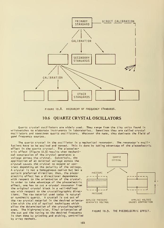
PRIMARYSTANDARD
DIRECT CALIBRATION
I
CALIBRATION
SECONDARYSTANDARDS
OTHERSTANDARDS
FIGURE 10.8. HIERARCHY OF FREQUENCY STANDARDS.
1 0.6 QUARTZ CRYSTAL OSCILLATORS
QUARTZ
CRYSTAL
PRESSURE
Quartz crystal oscillators are widely used. They range from the tiny units found in
wristwatches to elaborate instruments in laboratories. Sometimes they are called crystaloscillators and sometimes quartz oscillators. Whatever the name, they dominate the field ofgood frequency sources.
The quartz crystal in the oscillator is a mechanical resonator. The resonator's oscil-lations have to be excited and sensed. This is done by taking advantage of the piezoelectriceffect in the quartz crystal. The piezoelec-tric effect (figure 10.9) results when mechani-cal compression of the crystal generates a
voltage across the crystal. Conversely, the
application of an external voltage across the
crystal causes the crystal to expand or con-tract depending on the polarity of the voltage.A crystal is not a homogeneous medium but has a
certain preferred direction; thus, the piezo-electric effect has a directional dependencewith respect to the orientation of the crystal.In order to take advantage of the piezoelectriceffect, one has to cut a crystal resonator from
the original crystal block in a well-definedway with respect to the crystal lographic direc-tions. The raw material used today is natural
or synthetic quartz. A crystal is cut out of
the raw crystal material in the desired orienta-tion with the aid of optical techniques whichallow the determination of the crystal lographicaxes. The high-precision, final orientation of
the cut and the tuning to the desired frequencyis then done by grinding and etching, controlledby x-ray methods.
164
++++++++++++++
PRESSURE
APPLIED PRESSUREGENERATES VOLTAGE
l 1
1
(i
?
i i
APPLIED VOLTAGECAUSES CONTRACTION
FIGURE 10.9- THE PIEZOELECTRIC EFFECT.
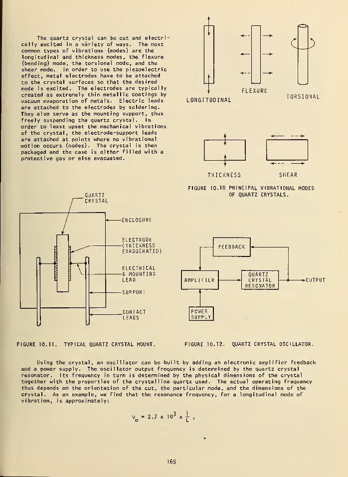
The quartz crystal can be cut and electri-
cally excited in a variety of ways. The mostcommon types of vibrations (modes) are the
longitudinal and thickness modes, the flexure(bending) mode, the torsional mode, and theshear mode. In order to use the piezoelectriceffect, metal electrodes have to be attached
to the crystal surfaces so that the desired
mode is excited. The electrodes are typically
created as extremely thin metallic coatings by
vacuum evaporation of metals. Electric leads
are attached to the electrodes by soldering.
They also serve as the mounting support, thus
freely suspending the quartz crystal. In
order to least upset the mechanical vibrationsof the crystal, the electrode-support leads
are attached at points where no vibrationalmotion occurs (nodes). The crystal is then
packaged and the case is either filled with a
protective gas or else evacuated.
"
C_3
FLEXURE
LONGITUDINALTORSIONAL
THICKNESS SHEAR
QUARTZCRYSTAL
\
-ENCLOSURE
electrode-(thicknessexaggerated;
ELECTRICAL-& MOUNTINGLEAD
-SUPPORT
CONTACTLEADS
FIGURE 10.10 PRINCIPAL VIBRATIONAL MODESOF QUARTZ CRYSTALS.
ccrncnri/
'1
AMPLIFIERQUARTZCRYSTAL
RESONATORi
POWERSUPPLY
OUTPUT
FIGURE 10.11. TYPICAL QUARTZ CRYSTAL MOUNT. FIGURE 10.12. QUARTZ CRYSTAL OSCILLATOR.
Using the crystal, an oscillator can be built by adding an electronic amplifier feedbackand a power supply. The oscillator output frequency is determined by the quartz crystalresonator. Its frequency in turn is determined by the physical dimensions of the crystaltogether with the properties of the crystalline quartz used. The actual operating frequencythus depends on the orientation of the cut, the particular mode, and the dimensions of the
crystal. As an example, we find that the resonance frequency, for a longitudinal mode of
vibration, is approximately:
vQ
= 2.7 10-1
XL
165
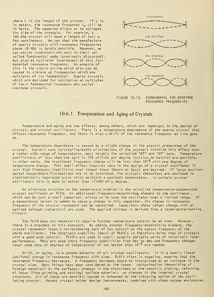
where L is the length of the crystal. If L is
in meters, the resonance frequency vQ will be
in hertz. The equation allows us to estimatethe size of the crystals. For example, a
100 kHz crystal will have a length of just a
few centimeters. We see that the manufactureof quartz crystals with resonance frequenciesabove 10 MHz is hardly possible. However, we
can excite resonators not only in their so-
called fundamental mode (previously discussed),but also at multiples (overtones) of this fun-damental resonance frequency. An example of
this is the violin string which also can be
caused to vibrate at frequencies which aremultiples of its fundamental. Quartz crystalswhich are designed for excitation at multiplesof their fundamental resonance are calledovertone crystals.
FUNDAMENTAL
2nd OVERTONE
4tn OVERTONE
FIGURE 10.13. FUNDAMENTAL AND OVERTONERESONANCE FREQUENCIES.
1 0.6. 1 Temperature and Aging of Crystals
Temperature and aging are two effects, among others, which are important in the design of
crystals and crystal oscillators. There is a temperature dependence of the quartz crystal thataffects resonance frequency, and there is also a drift of the resonance frequency as time goeson
.
The temperature dependence is caused by a slight change in the elastic properties of thecrystal. Certain cuts (crystal lographic orientations of the crystal) minimize this effect overa rather wide range of temperatures, most notably the so-called "AT" and "GT" cuts. Temperaturecoefficients of less than one part in 100 million per degree (celsius or kelvin) are possible.In other words, the fractional frequency change will be less than 10"° with one degree of
temperature change. This small effect requires care in the design of a crystal oscillator if
very high frequency stabilities over longer times (hours or days) are desired. If large environ-mental temperature fluctuations are to be tolerated, the crystals themselves are enclosed in
electronically regulated ovens which maintain a constant temperature. In certain crystaloscillators this is done to better than 1/1000 of a degree.
An alternate solution to the temperature problem is the so-called temperature-compensatedcrystal oscillator or TCX0. An additional frequency-determining element in the oscillator,which can be just a small capacitor, allows us to tune the oscillator over a limited range. If
a temperature sensor is added to cause a change in this capacitor, the change in resonancefrequency of the crystal resonator can be cancelled. Capacitors whose values change with an
applied voltage (varactors) are used. The applied voltage is derived from a temperature-sensingc i rcui t
.
The TC X does not necessarily require further temperature control by an oven. However,there is a drawback to this approach. By adding another frequency-determining element, the
crystal resonator loses a corresponding part of its control on the output frequency of the
whole oscillator. The long-term stability (days) of TCXO's is therefore below that of crystalswith a good oven control. TCXO's are used in small, usually portable units of relatively lower
performance. They are used where frequency stabilities from day to day and frequency changes
(over some tens of degrees of temperature) of not better than 10"9 are needed.
Drift, or aging, is a common behavior of all crystal oscillators. It is a nearly linear
(uniform) change in resonance frequency with time. Drift often is negative, meaning that the
resonance frequency decreases. A frequency decrease could be interpreted as an increase in the
crystal size. Many things have been considered as the cause: contamination (depositing of
foreign material) on the surfaces; changes in the electrodes or the metallic plating; reforming
of loose (from grinding and etching) surface material; or changes in the internal crystal
structure. All of these are possibly caused or enhanced by the vibrating motion of the oscil-
lating crystal. Recent crystal holder design improvements, combined with clean vacuum enclosures,
166
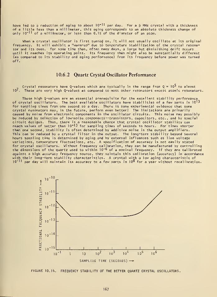
have led to a reduction of aging to about 10"'' per day. For a 5 MHz crystal with a thicknessof a little less than a millimeter, this aging corresponds to an absolute thickness change of
only 10~'' of a millimeter, or less than 0.1% of the diameter of an atom.
When a crystal oscillator is first turned on, it will not usually oscillate at its originalfrequency. It will exhibit a "warm-up" due to temperature stabilization of the crystal resona-tor and its oven. For some time then, often many days, a large but diminishing drift occursuntil it reaches its operating point. Its frequency then might also be substantially different(as compared to its stability and aging performance) from its frequency before power was turnedoff.
10.6.2 Quartz Crystal Oscillator Performance
Crystal resonators have Q-values which are typically in the range from Q = lO-' to almost10'. These are very high Q_-values as compared to most other resonators except atomic resonators.
These high Q-values are an essential prerequisite for the excellent stability performanceof crystal oscillators. The best available oscillators have stabilities of a few parts in 10'3
for sampling times from one second to a day. There is some experimental evidence that somecrystal resonators may, in the future, perform even better! The limitations are primarilycaused by noise from electronic components in the oscillator circuits. This noise may possiblybe reduced by selection of low-noise components--trans i stors , capacitors, etc., and by specialcircuit designs. Thus, there is a reasonable chance that crystal oscillator stability canreach values of better than 10~'3 for sampling times of seconds to hours. For times shorterthan one second, stability is often determined by additive noise in the output amplifiers.This can be reduced by a crystal filter in the output. The long-term stability beyond severalhours sampling time is determined by aging and by external influences such as line voltagevariations, temperature fluctuations, etc. A specification of accuracy is not easily statedfor crystal oscillators. Without frequency calibration, they can be manufactured by controllingthe dimensions of the quartz used to within 10"° of a nominal frequency. If they are calibratedagainst a high accuracy frequency source, they maintain this calibration (accuracy) in accordancewith their long-term stability characteristics. A crystal with a low aging characteristic of10"'' per day will maintain its accuracy to a few parts in 10° for a year without recal ibrat ion
.
10-10
10•1 1
io-12 -
10•13
•14
10-15
10" 1
1
7 3 410 10 10 10 10
510
6
SAMPLING TIME (SECONDS) —*
FIGURE 10. 14. FREQUENCY STABILITY OF THE BETTER QUARTZ CRYSTAL OSCILLATORS,
167
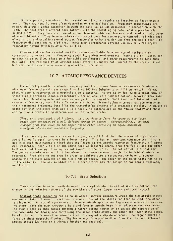
It is apparent, therefore, that crystal oscillators require calibration at least once a
year. They may need it more often depending on the application. Frequency adjustments aremade with a small added capacitor in much the same way as was discussed in connection with theTCXO. The most stable crystal oscillators, with the lowest aging rate, cost approximately$2,000 (1975). They have a volume of a few thousand cubic centimeters, and require input powerof about 10 watts. They have an elaborate crystal oven for temperature control, wel
1
-designedelectronics, and usually several output frequencies which are derived from the oscillator withfrequency dividers and multipliers. These high performance devices use 2.5 or 5 MHz crystalresonators having Q-values of a few million.
Cheaper and smaller crystal oscillators are available in a variety of designs withcorresponding reductions in frequency stability and/or environmental insensi tivi ty . Costs cango down to below $100, sizes to a few cubic centimeters, and power requirements to less than0.1 watt. The reliability of crystal oscillators is usually not limited by the crystal itself,but also depends on the accompanying electronic circuits.
10.7 ATOMIC RESONANCE DEVICES
Commercially available atomic frequency oscillators are based on resonances in atoms atmicrowave f requencies--in the range from 1 to 100 GHz (gigahertz or billion hertz). We maypicture atomic resonance as a magnetic dipole antenna. We typically deal with a great many ofthese dipole antennas (atomic resonators), and we can, as a simplification, separate them intotwo kinds: Receiving antennas receive energy from a magnetic field that oscillates at theirresonance frequency, much like a TV antenna at home. Transmitting antennas radiate energy attheir resonance frequency just like the transmitting antenna of a broadcast station. A physicistmight say that the atoms that act like a receiving antenna are in the "lower state" and thoseacting like a transmitting antenna are in the "upper state."
There is a peculiarity with atoms: an atom changes from the upper to the lowerstate upon emission of a well-defined amount of energy. Correspondingly , an atomchanges from the lower to the upper state after receiving an equal amount ofenergy at the atomic resonance frequency.
If we have a great many atoms as in a gas, we will find that the number of upper stateatoms is nearly equal to those in a lower state. This has an important consequence: If thisgas is placed in a magnetic field that oscillates at the atomic resonance frequency, all atomswill resonate. Nearly half of the atoms receive (absorb) energy from the field, and the otherhalf emit (add) energy of an equivalent amount to the field. The net effect is almost zero.
The gas as a whole acts as if it has almost no resonance even though the individual atoms do
resonate. From this we see that in order to achieve atomic resonance, we have to somehow
change the relative amounts of the two kinds of atoms. The upper or the lower state has to be
in the majority. The way in which this is done determines the design of our atomic frequency
osci 1 lator.
10.7.1 State Selection
There are two important methods used to accomplish what is called state selection—thechange in the relative numbers of the two kinds of atoms (upper state and lower state):
Spatial state selection relies on an actual sorting procedure where the two atomic states
are sorted into different directions in space. One of the states can then be used; the other
is discarded. An actual system may produce an atomic gas by heating some substance in an oven.
The atoms leave the oven through a hole and form an atomic beam in an adjacent vacuum chamber.
The atomic beam is then passed through a rather strong magnet which causes the separation of
the beam into two beams, one containing the upper state atoms, the other the lower state atoms.
Recall that our picture of an atom is that of a magnetic dipole antenna. The magnet exerts a
force on these magnetic dipoles. The force acts in opposite directions for the two different
atomic states (we note this without further explanation).
168
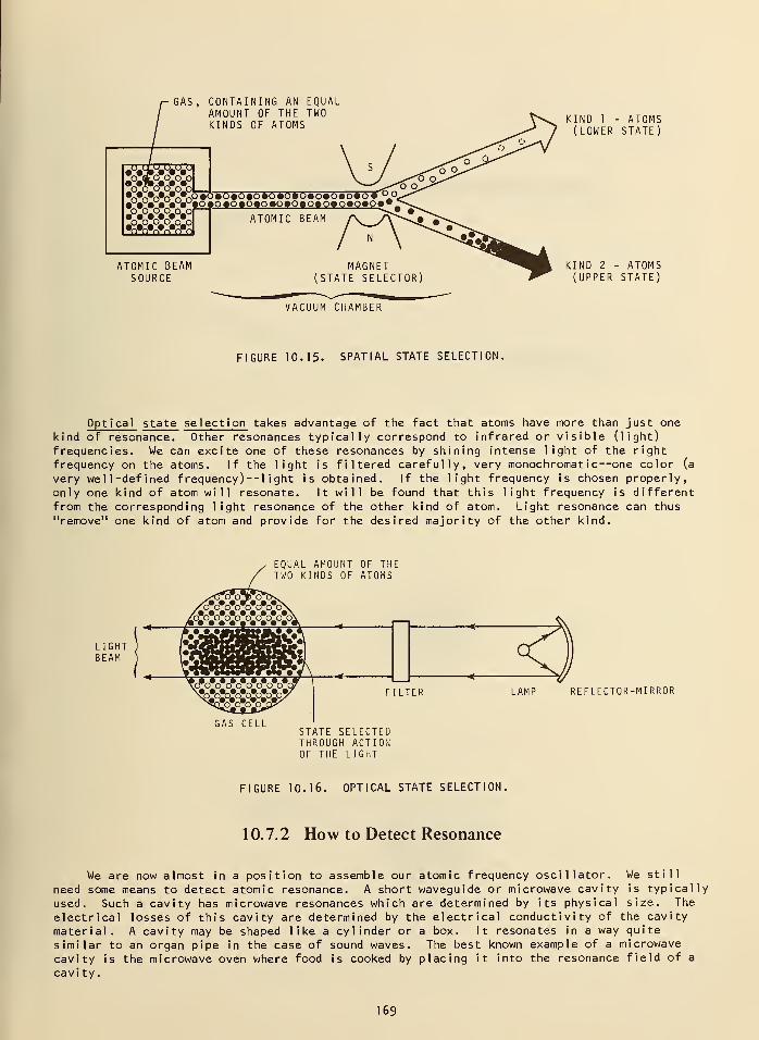
GAS, CONTAINING AN EQUALAMOUNT OF THE TWOKINDS OF ATOMS
o <~> crcfo ol—SM££B#^282>2*2&teS2S2S2S2*.
Jojooooot° o»oto»o>o>o«o«oto«o>ot '
ATOMIC BEAMSOURCE
ATOMIC BEAM
KIND 1 - ATOMS(LOWER STATE)
MAGNET(STATE SELECTOR
KIND 2 - ATOMS(UPPER STATE)
VACUUM CHAMBER
FIGURE 10.15. SPATIAL STATE SELECTION.
Optical state selection takes advantage of the fact that atoms have more than just one
kind of resonance. Other resonances typically correspond to infrared or visible (light)
frequencies. We can excite one of these resonances by shining intense light of the right
frequency on the atoms. If the light is filtered carefully, very monochromat ic--one color (a
very well-defined f requency)--l ight is obtained. If the light frequency is chosen properly,
only one kind of atom will resonate. It will be found that this light frequency is differentfrom the corresponding light resonance of the other kind of atom. Light resonance can thus
"remove" one kind of atom and provide for the desired majority of the other kind.
EQUAL AMOUNT OF THETWO KINDS OF ATOMS
STATE SELECTEDTHROUGH ACTIONOF THE LIGHT
FILTER LAMP REFLECTOR-MIRROR
FIGURE 10.16. OPTICAL STATE SELECTION.
10.7.2 How to Detect Resonance
We are now almost in a position to assemble our atomic frequency oscillator. We still
need some means to detect atomic resonance. A short waveguide or microwave cavity is typically
used. Such a cavity has microwave resonances which are determined by its physical size. The
electrical losses of this cavity are determined by the electrical conductivity of the cavity
material. A cavity may be shaped like a cylinder or a box. It resonates in a way quite
similar to an organ pipe in the case of sound waves. The best known example of a microwave
cavity is the microwave oven where food is cooked by placing it into the resonance field of a
cavity.
169
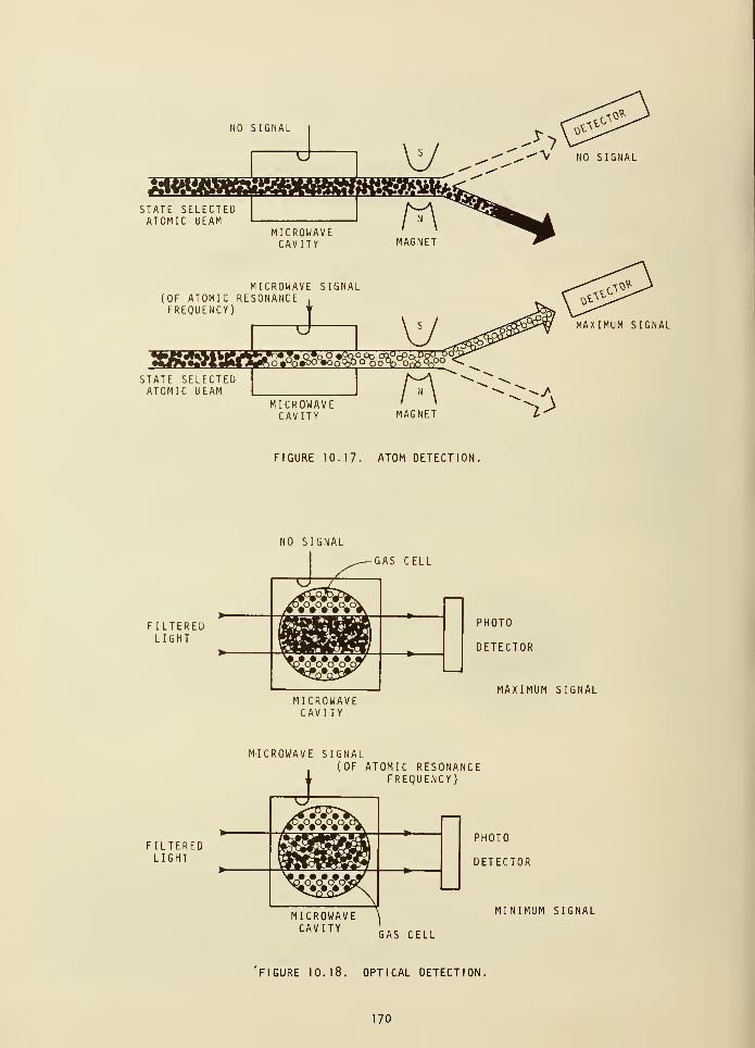
NO SIGNAL
tfeftfc>ttgrtWTATE SELECTED
ig^Bfgygja^g^j^gegcgQffgjxiSTATE SELECTEDATOMIC BEAM
MICROWAVECAVITY
IAMAGNET
MAXIMUM SIGNAL
~f>
FIGURE 10.17. ATOM DETECTION,
NO SIGNAL
FILTEREDLIGHT
^— GAS CELL
4$&&
^wMICROWAVECAVITY
PHOTO
DETECTOR
MAXIMUM SIGNAL
FILTEREDLIGHT
MICROWAVE SIGNAL(OF ATOMIC RESONANCE
1 FREQUENCY)
/4www^
**S^?MICROWAVECAVITY
PHOTO
DETECTOR
MINIMUM SIGNAL
GAS CELL
FIGURE 10.18. OPTICAL DETECTION.
170
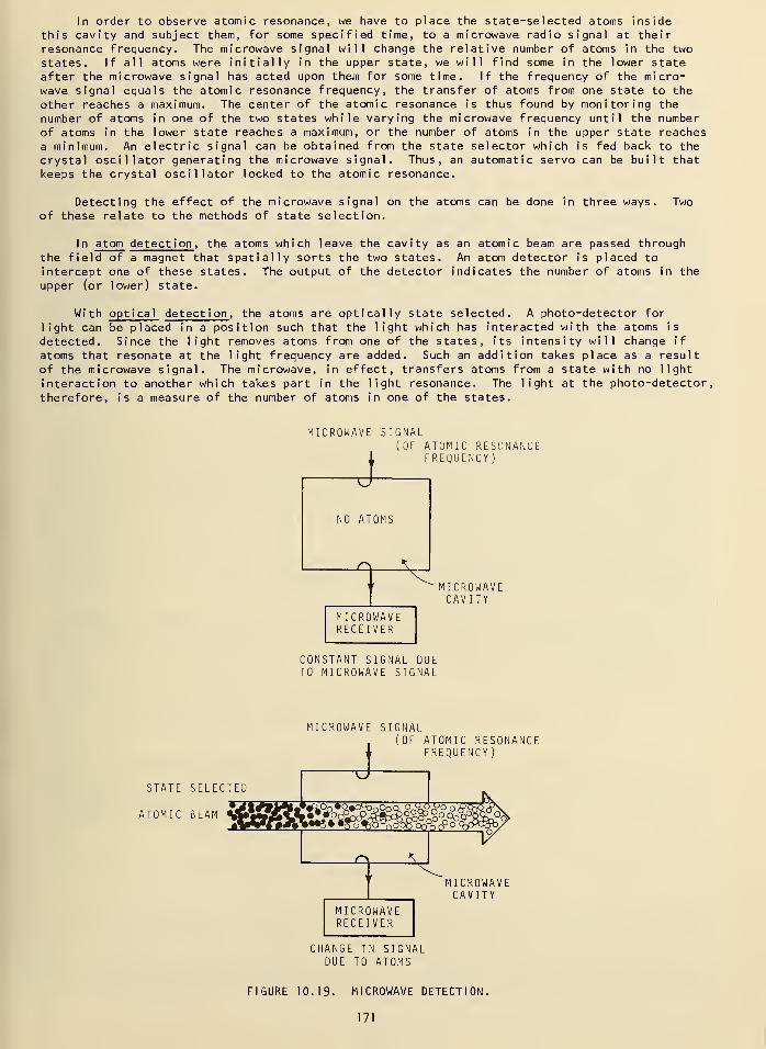
In order to observe atomic resonance, we have to place the state-selected atoms inside
this cavity and subject them, for some specified time, to a microwave radio signal at theirresonance frequency. The microwave signal will change the relative number of atoms in the two
states. If all atoms were initially in the upper state, we will find some in the lower stateafter the microwave signal has acted upon them for some time. If the frequency of the micro-wave signal equals the atomic resonance frequency, the transfer of atoms from one state to the
other reaches a maximum. The center of the atomic resonance is thus found by monitoring the
number of atoms in one of the two states while varying the microwave frequency until the numberof atoms in the lower state reaches a maximum, or the number of atoms in the upper state reachesa minimum. An electric signal can be obtained from the state selector which is fed back to the
crystal oscillator generating the microwave signal. Thus, an automatic servo can be built that
keeps the crystal oscillator locked to the atomic resonance.
Detecting the effect of the microwave signal on the atoms can be done in three ways. Twoof these relate to the methods of state selection.
In atom detection , the atoms which leave the cavity as an atomic beam are passed throughthe field of a magnet that spatially sorts the two states. An atom detector is placed to
intercept one of these states. The output of the detector indicates the number of atoms in the
upper (or lower) state.
With optical detection , the atoms are optically state selected. A photo-detector for
light can be placed in a position such that the light which has interacted with the atoms is
detected. Since the light removes atoms from one of the states, its intensity will change if
atoms that resonate at the light frequency are added. Such an addition takes place as a resultof the microwave signal. The microwave, in effect, transfers atoms from a state with no light
interaction to another which takes part in the light resonance. The light at the photo-detector,therefore, is a measure of the number of atoms in one of the states.
MICROWAVE SIGNAL(OF ATOMIC RESONANCE
FREQUENCY)
"O
NO ATOMS
MICROWAVECAVITY
MICROWAVERECEIVER
CONSTANT SIGNAL DUETO MICROWAVE SIGNAL
MICROWAVE SIGNAL(OF ATOMIC RESONANCE
FREQUENCY
STATE SELECTED
ATOMIC BEAM
MICROWAVECAVITY
CHANGE IN SIGNALDUE TO ATOMS
FIGURE 10. 19- MICROWAVE DETECTION.
171
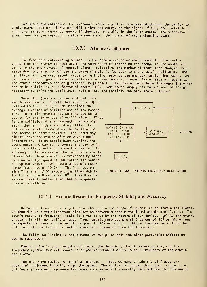
For microwave detection , the microwave radio signal is transmitted through the cavity toa microwave detector. The atoms will either add energy to the signal if they are initially in
the upper state or subtract energy if they are initially in the lower state. The microwavepower level at the detector is thus a measure of the number of atoms changing state.
10.7.3 Atomic Oscillators
The frequency-determining element is the atomic resonator which consists of a cavitycontaining the state-selected atoms and some means of detecting the change in the number ofatoms in the two states. A control signal, related to the number of atoms that changed theirstate due to the action of the microwave signal, is fed back to the crystal oscillator. Theoscillator and the associated frequency multiplier provide the energy-transferring means. Asdiscussed before, good crystal oscillators are available at frequencies of several megahertz.The atomic resonances are at gigahertz frequencies. The crystal oscillator frequency thereforehas to be multiplied by a factor of about 1000. Some power supply has to provide the energynecessary to drive the oscillator, multiplier, and possibly the atom state selector.
Very high Q. values can be achieved withatomic resonators. Recall that resonator Q is
related to the time T, which describes the
average duration of oscillations of the resona-tor. In atomic resonators, we find two chief
causes for the dying out of oscillations. Firstis the collision of the resonating atoms with
each other and with surrounding walls. Each
collision usually terminates the oscillation.The second is rather obvious. The atoms maysimply leave the region of microwave signal
interaction. In an atomic beam machine, the
atoms enter the cavity, traverse the cavity in
a certain time, and then leave the cavity. As
an example, let us assume that we have a cavityof one meter length which is traversed by atoms
with an average speed of 100 meters per second
(a typical value). We assume an atomic reso-
nance frequency of 10 GHz. The interactiontime T is then 1/100 second, the linewidth is
100 Hz, and the 0. value is 10°. This 0_ valueis considerably better than that of a quartzcrystal oscillator.
'
QUARTZ CRYSTALOSCILLATOR
AND FREQUENCYMULTIPLIER
ATOMICRESONATOR
J i
POWERSUPPLY
•-OUTPUT
FIGURE 10.20. ATOMIC FREQUENCY OSCILLATOR.
10.7.4 Atomic Resonator Frequency Stability and Accuracy
Before we discuss what might cause changes in the output frequency of an atomic oscillator,we should make a very important distinction between quartz crystal and atomic oscillators: The
atomic resonance frequency itself is given to us by the nature of our device. Unlike the quartz
crystal, it will not drift or age. Thus, atomic resonators with Q values of 10°> or higher may
be expected to have accuracies of one part in 10° or better. This is because we will not be
able to shift the frequency further away from resonance than the linewidth.
The following listing is not exhaustive but gives only the minor perturbing effects on
atomic resonators:
Random noise in the crystal oscillator, the detector, the microwave cavity, and the
frequency synthesizer will cause corresponding changes of the output frequency of the atomic
osci 1 lator.
The microwave cavity is itself a resonator. Thus, we have an additional frequency-determining element in addition to the atoms. The cavity influences the output frequency by
pulling the combined resonance frequency to a value which usually lies between the resonances
172
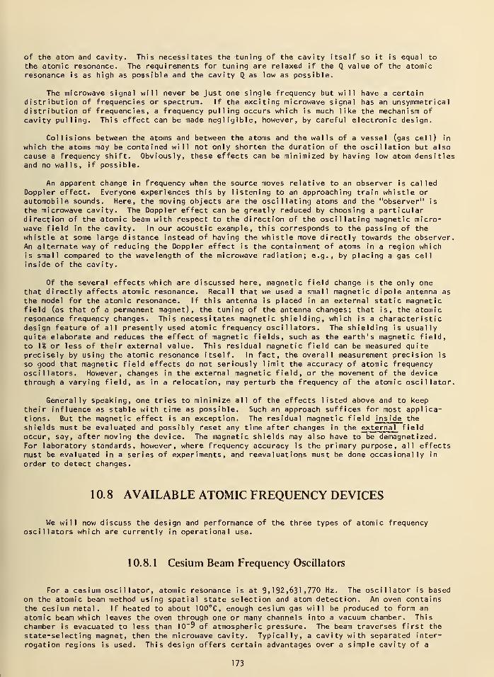
of the atom and cavity. This necessitates the tuning of the cavity itself so it is equal to
the atomic resonance. The requirements for tuning are relaxed if the Q value of the atomicresonance is as high as possible and the cavity Q_ as low as possible.
The microwave signal will never be just one single frequency but will have a certaindistribution of frequencies or spectrum. If the exciting microwave signal has an unsymmetr ical
distribution of frequencies, a frequency pulling occurs which is much like the mechanism ofcavity pulling. This effect can be made negligible, however, by careful electronic design.
Collisions between the atoms and between the atoms and the walls of a vessel (gas cell) in
which the atoms may be contained will not only shorten the duration of the oscillation but alsocause a frequency shift. Obviously, these effects can be minimized by having low atom densitiesand no walls, if possible.
An apparent change in frequency when the source moves relative to an observer is calledDoppler effect. Everyone experiences this by listening to an approaching train whistle orautomobile sounds. Here, the moving objects are the oscillating atoms and the "observer" is
the microwave cavity. The Doppler effect can be greatly reduced by choosing a particulardirection of the atomic beam with respect to the direction of the oscillating magnetic micro-wave field in the cavity. In our acoustic example, this corresponds to the passing of thewhistle at some large distance instead of having the whistle move directly towards the observer.An alternate way of reducing the Doppler effect is the containment of atoms in a region whichis small compared to the wavelength of the microwave radiation; e.g., by placing a gas cell
inside of the cavity.
Of the several effects which are discussed here, magnetic field change is the only onethat directly affects atomic resonance. Recall that we used a small magnetic dipole antenna as
the model for the atomic resonance. If this antenna is placed in an external static magneticfield (as that of a permanent magnet), the tuning of the antenna changes; that is, the atomicresonance frequency changes. This necessitates magnetic shielding, which is a characteristicdesign feature of all presently used atomic frequency oscillators. The shielding is usuallyquite elaborate and reduces the effect of magnetic fields, such as the earth's magnetic field,
to \% or less of their external value. This residual magnetic field can be measured quiteprecisely by using the atomic resonance itself. In fact, the overall measurement precision is
so good that magnetic field effects do not seriously limit the accuracy of atomic frequencyoscillators. However, changes in the external magnetic field, or the movement of the devicethrough a varying field, as in a relocation, may perturb the frequency of the atomic oscillator.
Generally speaking, one tries to minimize all of the effects listed above and to keeptheir influence as stable with time as possible. Such an approach suffices for most applica-tions. But the magnetic effect is an exception. The residual magnetic field inside the
shields must be evaluated and possibly reset any time after changes in the external fieldoccur, say, after moving the device. The magnetic shields may also have to be demagnetized.For laboratory standards, however, where frequency accuracy is the primary purpose, all effectsmust be evaluated in a series of experiments, and reevaluat ions must be done occasionally in
order to detect changes.
10.8 AVAILABLE ATOMIC FREQUENCY DEVICES
We will now discuss the design and performance of the three types of atomic frequencyoscillators which are currently in operational use.
10.8.1 Cesium Beam Frequency Oscillators
For a cesium oscillator, atomic resonance is at 9.192,631,770 Hz. The oscillator is based
on the atomic beam method using spatial state selection and atom detection. An oven containsthe cesium metal. If heated to about 100°C, enough cesium gas will be produced to form an
atomic beam which leaves the oven through one or many channels into a vacuum chamber. This
chamber is evacuated to less than 10"9 of atmospheric pressure. The beam traverses first the
state-selecting magnet, then the microwave cavity. Typically, a cavity with separated inter-
rogation regions is used. This design offers certain advantages over a simple cavity of a
173
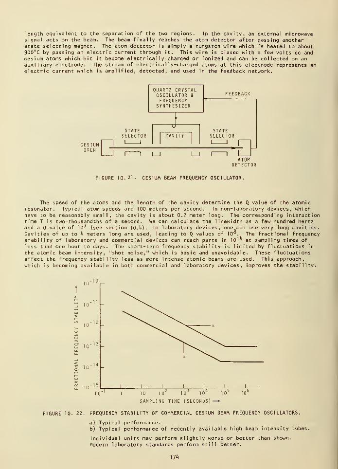
length equivalent to the separation of the two regions. In the cavity, an external microwavesignal acts on the beam. The beam finally reaches the atom detector after passing anotherstate-selecting magnet. The atom detector is simply a tungsten wire which is heated to about900°C by passing an electric current through it. This wire is biased with a few volts dc andcesium atoms which hit it become electrical ly» charged or ionized and can be collected on anauxiliary electrode. The stream of electrically-charged atoms at this electrode represents anelectric current which is amplified, detected, and used in the feedback network.
QUARTZ CRYSTALOSCILLATOR & FEEDBACK
FREQUENCYSYNTHESIZER
"
STATESELECTOR
VSTATE
CAVITY SELECTOR[ |
1 '1CES IUM 1
OVEN1 1 1 L_l L_l 1 1 1
ATOMDETECTOR
FIGURE 10.21. CESIUM BEAM FREQUENCY OSCILLATOR.
The speed of the atoms and the length ofresonator. Typical atom speeds are 100 metershave to be reasonably small, the cavity is abotime T is two-thousandths of a second. We canand a Q. value of 10? (see section 10.4). In la
Cavities of up to k meters long are used, lead
stability of laboratory and commercial devicesless than one hour to days. The short-term fr
the atomic beam intensity, "shot noise," whichaffect the frequency stability less as more in
which is becoming available in both commercial
the cavity determine the Q value of the atomicper second. In non-laboratory devices, which
ut 0.2 meter long. The corresponding interactioncalculate the linewidth as a few hundred hertzboratory devices, one can use very long cavities,ing to Q values of 10 . The fractional frequencycan reach parts in 10^ at sampling times of
equency stability is limited by fluctuations in
is basic and unavoidable. These fluctuationstense atomic beams are used. This approach,and laboratory devices, improves the stability.
10- 10r-
o-n
r-
10c
io-13 -
10
£ 10-lb
10 10 10 10
SAMPLING TIME (SECONDS)
10'
FIGURE 10. 22. FREQUENCY STABILITY OF COMMERCIAL CESIUM BEAM FREQUENCY OSCILLATORS.
a) Typical performance.b) Typical performance of recently available high beam intensity tubes.
Individual units may perform slightly worse or better than shown.
Modern laboratory standards perform still better.
174
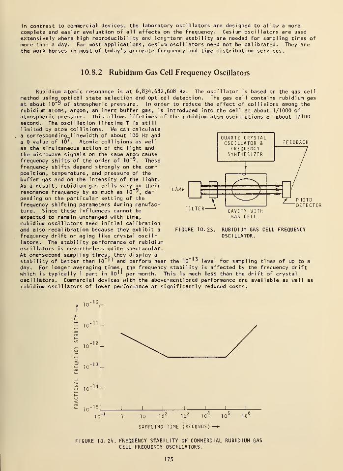
In contrast to commercial devices, the laboratory oscillators are designed to allow a morecomplete and easier evaluation of all effects on the frequency. Cesium oscillators are used
extensively where high reproducibility and long-term stability are needed for sampling times ofmore than a day. For most applications, cesium oscillators need not be calibrated. They are
the work horses in most of today's accurate frequency and time distribution services.
10.8.2 Rubidium Gas Cell Frequency Oscillators
QUARTZ CRYSTALOSCILLATOR &
FREQUENCYSYNTHESIZER
FEEDBACK
LAMP
FILTER_A
Rubidium atomic resonance is at 6,83^,682,608 Hz. The oscillator is based on the gas cell
method using optical state selection and optical detection. The gas cell contains rubidium gas
at about 10~° of atmospheric pressure. In order to reduce the effect of collisions among therubidium atoms, argon, an inert buffer gas, is introduced into the cell at about 1/1000 ofatmospheric pressure. This allows lifetimes of the rubidium atom oscillations of about 1/100second. The oscillation lifetime T is still
limited by atom collisions. We can calculatea corresponding 1 inewidth of about 100 Hz and
a Q value of 10. Atomic collisions as well
as the simultaneous action of the light and
the microwave signals on the same atom causefrequency shifts of the order of 10"°. Thesefrequency shifts depend strongly on the com-
position, temperature, and pressure of the
buffer gas and on the intensity of the light.
As a result, rubidium gas cells vary in theirresonance frequency by as much as 10"°, de-
pending on the particular setting of the
frequency shifting parameters during manufac-ture. Since these influences cannot be
expected to remain unchanged with time,
rubidium osci I lators need initial calibrationand also recal ibrat ion because they exhibit a
frequency drift or aging like crystal oscil-lators. The stability performance of rubidiumoscillators is nevertheless quite spectacular.At one-second sampling times, they display a
stability of better than 10"'' and perform near the 10" '^ level for sampling times of up to a
day. For longer averaging times, the frequency stability is affected by the frequency drift
which is typically 1 part in 10'' per month. This is much less than the drift of crystaloscillators. Commercial devices with the above-mentioned performance are available as well as
rubidium oscillators of lower performance at significantly reduced costs.
FIGURE 10. 23.
CAVITY WITHGAS CELL
RUBIDIUM GAS CELL FREQUENCYOSCILLATOR.
o-10
,-
10
o-12 -
1013
-14
,-1 5
1
_L _L J_
10 10 10 10
SAMPLING TIME (SECONDS)
10
IGURE 10. 2k. FREQUENCY STABILITY OF COMMERCIAL RUBIDIUM GAS
CELL FREQUENCY OSCILLATORS.
175
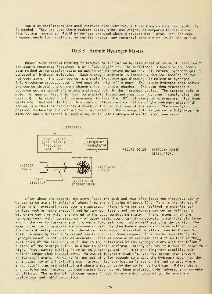
Rubidium oscillators are used wherever excellent med ium- term- -minutes to a day-stabilityis needed. They are used where reduced costs, size, and weight, as compared to cesium oscil-lators, are important. Rubidium devices are used where a crystal oscillator, with its morefrequent needs for recal ibrat ion and its greater environmental sensitivity, would not suffice.
10.8.3 Atomic Hydrogen Masers
Maser is an acronym meanThe atomic resonance frequencbeam method using spatial stacomposed of hydrogen moleculehydrogen atoms. The beam sou
This discharge produces atomi
the source through one or manstate-selecting magnet and en
made from quartz glass whichcavity Q_. The storage bulb i
walls are lined with Teflon,the walls without significantphysical mechanisms are not ydiameter and dimensioned in s
i ng "microwave amplification by stimulated emission of radiation."y is at 1,^20,405,752 Hz. The oscillator is based on the atomicte selection and microwave detection. All natural hydrogen gas is
s. Each hydrogen molecule is formed by chemical bonding of tworce is a radio frequency gas discharge in molecular hydrogen,c hydrogen with high efficiency. The atomic hydrogen beam leaves
y channels into a vacuum chamber. The beam then traverses a
ters a storage bulb in the microwave cavity. The storage bulb is
has low electric losses and thus does not significantly alter thes evacuated to less than 10"!
' of atmospheric pressure. Its innerThis coating allows many collisions of the hydrogen atoms with
ly disturbing the oscillations of the atoms. The underlyinget fully understood. The storage bulb is typically 0.15 meter in
uch a way as to hold hydrogen atoms for about one second.
FEEDBACK
lYDROGENSOURCE
FIGURE 10.25- HYDROGEN MASEROSCILLATOR.
CAVITY WITHSTORAGE BULb
After about one second, the atoms leave the bulb and thus also leave the microwave cavity.
We can calculate a linewidth of about 1 Hz and a Q. value of about 109. This is the highest 0_
value in all presently-used atomic standards. Higher Q values are realized in experimentaldevices such as methane-stabilized helium-neon lasers and ion storage devices as well as in
microwave cavities which are cooled to the superconducting state. If the intensity of the
hydrogen beam, which consists only of upper state atoms (emitting atoms), is sufficiently large
and if the cavity losses are sufficiently low, self-oscillation will start in the cavity. The
maser itself will generate a microwave signal. We then have a maser-osci 1 lator with an outputfrequency directly derived from the atomic resonance. A crystal oscillator can be locked to
this frequency by frequency comparison techniques. When compared to a cesium oscillator, the
hydrogen maser is not quite as accurate. This is because of experimental difficulties in the
evaluation of the frequency shift due to the collisions of the hydrogen atoms with the Teflon
surface of the storage bulb. In order to obtain self-oscillation, the cavity Q_ must be relativelyhigh. Thus, cavity pulling is relatively strong, and it limits the long-term stability over
periods longer than several days. Values of long-term stability are not better than those of
cesium oscillators. However, for periods of a few seconds to a day, the hydrogen maser has the
best stability of all existing oscillators. Its application is rather limited to uses where
these stabilities are critical and where a rather bulky device is not handicap. Unlike cesium
and rubidium oscillators, hydrogen masers have not yet been evaluated under adverse environmental
conditions. The number of hydrogen masers in use is very small compared to the numbers of
cesium beam and rubidium devices.
.TM
76
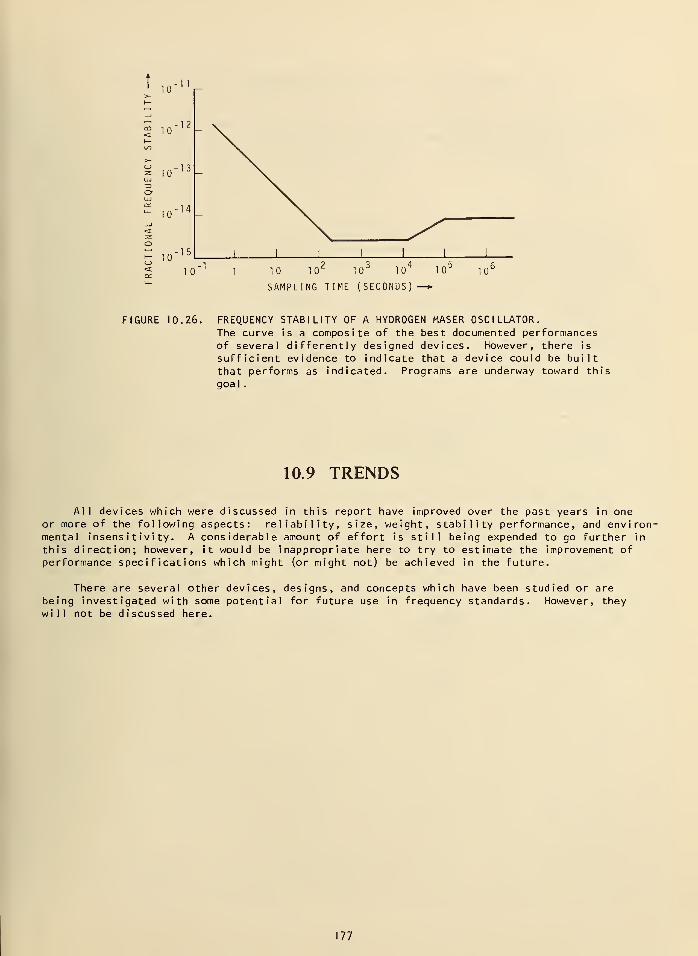
10 -
" ,„-15
10 10 10" 10J
10
SAMPLING TIME (SECONDS)
10' 10
FIGURE 10.26. FREQUENCY STABILITY OF A HYDROGEN MASER OSCILLATOR.The curve is a composite of the best documented performancesof several differently designed devices. However, there is
sufficient evidence to indicate that a device could be built
that performs as indicated. Programs are underway toward this
goal .
10.9 TRENDS
All devices which were discussed in this report have improved over the past years in oneor more of the following aspects: reliability, size, weight, stability performance, and environ-mental insensi
t
ivi ty. A considerable amount of effort is still being expended to go further in
this direction; however, it would be inappropriate here to try to estimate the improvement ofperformance specifications which might (or might not) be achieved in the future.
There are several other devices, designs, and concepts which have been studied or are
being investigated with some potential for future use in frequency standards. However, theywill not be discussed here.
177
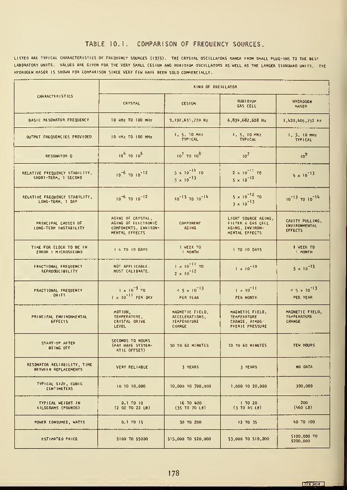
TABLE 10.1. COMPARISON OF FREQUENCY SOURCES.
LISTED ARE TYPICAL CHARACTERISTICS OF FREQUENCY SOURCES (1975). THE CRYSTAL OSCILLATORS RANGE FROM SMALL PLUG-INS TO THE BEST
LABORATORY UNITS. VALUES ARE GIVEN FOR THE VERY SMALL CESIUM AND RUBIDIUM OSCILLATORS AS WELL AS THE LARGER STANDARD UNITS. THE
HYDROGEN MASER IS SHOWN FOR COMPARISON SINCE VERY FEW HAVE BEEN SOLD COMMERCIALLY.
CHARACTERISTICS
KIND OF OSCILLATOR
CRYSTAL CESIUMRUBIDIUMGAS CELL
HYDROGENMASER
BASIC RESONATOR FREQUENCY 10 kHz TO 100 MHz 9,192,631 ,770 Hz 6, 83^, 682, 608 Hz 1 ,1*20, ^05, 752 Hz
OUTPUT FREQUENCIES PROVIDED 10 kHz TO 100 MHz 1 , 5, 10 MHzTYPICAL
1 , 5, 10 MHzTYPICAL
1 , 5, 10 MHzTYPICAL
RESONATOR QIt 6
10 TO 10 107
TO I08
107
I09
RELATIVE FREQUENCY STABILITY,SHORT-TERM, 1 SECOND
10"6 TO lO"'2 5 x 10"" TO
5x 10"' 3
2 x 10~'' TO
5x ,o"'2
5x ,0"' 3
RELATIVE FREQUENCY STABILITY,LONG-TERM, 1 DAY
I0"6
TO I0"'2
,
" ,3T0 lO""
1
-1 25 x 10 TO
3x ,0"' 3lO"'
3TO lO""
1
PRINCIPAL CAUSES OFLONG-TERM INSTABILITY
AGING OF CRYSTAL,AGING OF ELECTRONICCOMPONENTS, ENVIRON-MENTAL EFFECTS
COMPONENTAGING
LIGHT SOURCE AGING,FILTER & GAS CELLAGING, ENVIRON-MENTAL EFFECTS
CAVITY PULLING,ENVIRONMENTALEFFECTS
TIME FOR CLOCK TO BE IN
ERROR 1 MICROSECOND1 s TO 10 DAYS
1 WEEK TO1 MONTH
1 TO 10 DAYS1 WEEK TO
1 MONTH
FRACTIONAL FREQUENCYREPRODUCIBILITY
NOT APPLICABLE.MUST CALIBRATE.
1 x 10"" TO
2x lO"'2
1 x lO"' 5x 10"' 3
FRACTIONAL FREQUENCYDRIFT
1 x I0"9 TO
1 x 10"" PER DAY
< 5 x 10"' 3
PER YEAR
I x 10""
PER MONTH
< 5 x 10"' 3
PER YEAR
PRINCIPAL ENVIRONMENTALEFFECTS
MOT 1 ON
,
TEMPERATURE,CRYSTAL DRIVELEVEL
MAGNETIC FIELD,ACCELERATIONS,TEMPERATURECHANGE
MAGNETIC FIELD,TEMPEkATURECHANGE, ATMOS-PHERIC PRESSURE
MAGNETIC FIELD,TEMPERATURECHANGE
START-UP AFTERBEING OFF
SECONDS TO HOURS(MAY HAVE SYSTEM-ATIC OFFSET)
30 TO 60 MINUTES 10 TO 60 MINUTES FEW HOURS
RESONATOR RELIABILITY, TIMEBETWEEN REPLACEMENTS
VERY RELIABLE 3 YEARS 3 YEARS NO DATA
TYPICAL SIZE, CUBICCENTIMETERS
10 TO 10,000 10,000 TO 700,000 1 ,000 TO 20.000 300,000
TYPICAL WEIGHT IN
KILOGRAMS (POUNDS)0.1 TO 10
(2 OZ TO 22 LB)
16 TO itOO
(35 TO 70 LB)
1 TO 20
(3 TO 1*5 LB)
200Ci60 LB)
POWER CONSUMED, WATTS 0.1 TO 15 30 TO 200 12 TO 35 i.0 TO 100
ESTIMATED PRICE $100 TO $5000 $15,000 TO $20,000 $3,000 TO $10,000$100,000 TO
$200,000
178
[77X 3414
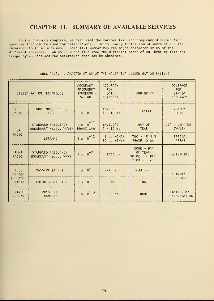
CHAPTER 11. SUMMARY OF AVAILABLE SERVICES
In the previous chapters, we discussed the various time and frequency dissemination
services that can be used for calibrations. The following tables should serve as a quickreference to these services. Table 11.1 summarizes the major characteristics of the
different services. Tables 11.2 and 11.3 show the different means of calibrating time and
frequency sources and the accuracies that can be obtained.
TABLE 1
1
CHARACTERISTICS OF THE MAJOR T&F DISSEMINATION SYSTEMS
i
DISSEMINATION TECHNIQUES
ACCURACYFREQUENCYSYNCHRONI-ZATION
ACCURACYFORDATE
TRANSFERAMBIGUITY
COVERAGEFOR
STATEDACCURACY
VLFRADIO
GBR, NBA, OMEGA,ETC. 1 x 10" n
ENVELOPE1
- 10 ms1 CYCLE
NEARLYGLOBAL
LF
RADIO
STANDARD FREQUENCYBROADCAST (e.g. , WWVB)
1 x lO"1 '
PHASE 24h
ENVELOPE1
- 10 ms
DAY OF
YEARUSA - LIMITED
(WWVB)
LORAN-C 5x 10" 12 1 ys (GND)
50 ys (SKY)
T0C -15 MIN
PHASE 10 ys
SPECIALAREAS
HF/MFRADIO
STANDARD FREQUENCYBROADCAST (e.g. , WWV)
1 x 10~ 71000 ys
CODE - DAY
OF YEARVOICE - 1 DAY
TICK - 1 s
HEMISPHERE
TELE-VISION(VHF/SHFRADIO
PASSIVE LINE-10 1 x lO"11
~1 ys -33 msNETWORKCOVERAGE
COLOR SUBCARRIER 1 x lO"11
NA NA
PORTABLECLOCKS
PHYSICALTRANSFER
1 x 10' 13100 ns NONE
LIMITED BY
TRANSPORTATION
179
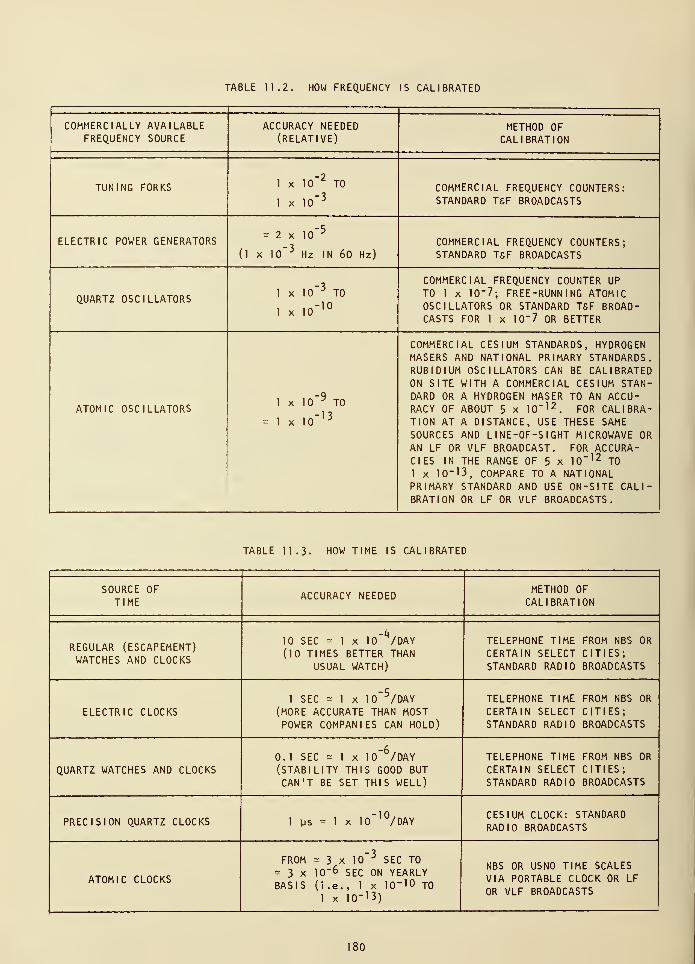
TABLE 11.2. HOW FREQUENCY IS CALIBRATED
COMMERCIALLY AVAILABLEFREQUENCY SOURCE
ACCURACY NEEDED(RELATIVE)
METHOD OF
CALIBRATION
TUNING FORKS 1 x 10" 2 TO
1 x 10" 3
COMMERCIAL FREQUENCY COUNTERS:STANDARD T&F BROADCASTS
ELECTRIC POWER GENERATORS= 2 x 10
_5
(1 x 10~ 3Hz IN 60 Hz)
COMMERCIAL FREQUENCY COUNTERS;STANDARD T&F BROADCASTS
QUARTZ OSCILLATORS1 x 10" 3
TO
1 x 10" 10
COMMERCIAL FREQUENCY COUNTER UP
TO 1 x 10⁻⁷; FREE-RUNNING ATOMICOSCILLATORS OR STANDARD T&F BROAD-CASTS FOR 1 x 10"7 OR BETTER
ATOMIC OSCILLATORS1 x 10" 9 TO
1 x ,0" 13
COMMERCIAL CESIUM STANDARDS, HYDROGENMASERS AND NATIONAL PRIMARY STANDARDS.RUBIDIUM OSCILLATORS CAN BE CALIBRATEDON SITE WITH A COMMERCIAL CESIUM STAN-DARD OR A HYDROGEN MASER TO AN ACCU-RACY OF ABOUT 5 x 1
0~n 2
. FOR CALIBRA-TION AT A DISTANCE, USE THESE SAMESOURCES AND L 1 NE-OF-S IGHT MICROWAVE ORAN LF OR VLF BROADCAST. FOR ACCURA-CIES IN THE RANGE OF 5 x 10" 12 TO
1 x 10-13, COMPARE TO A NATIONALPRIMARY STANDARD AND USE ON-SITE CALI-BRATION OR LF OR VLF BROADCASTS.
TABLE 11.3. HOW TIME IS CALIBRATED
SOURCE OFTIME
ACCURACY NEEDEDMETHOD OF
CALIBRATION
REGULAR (ESCAPEMENT)WATCHES AND CLOCKS
-k10 SEC = 1 x 10 /DAY
(10 TIMES BETTER THANUSUAL WATCH)
TELEPHONE TIME FROM NBS OR
CERTAIN SELECT CITIES;STANDARD RADIO BROADCASTS
ELECTRIC CLOCKS1 SEC = 1 x 10
_5/DAY
(MORE ACCURATE THAN MOSTPOWER COMPANIES CAN HOLD)
TELEPHONE TIME FROM NBS OR
CERTAIN SELECT CITIES;STANDARD RADIO BROADCASTS
QUARTZ WATCHES AND CLOCKS0.1 SEC - 1 x 10" /DAY(STABILITY THIS GOOD BUTCAN'T BE SET THIS WELL)
TELEPHONE TIME FROM NBS OR
CERTAIN SELECT CITIES;STANDARD RADIO BROADCASTS
PRECISION QUARTZ CLOCKS 1 ys = 1 x 10"'°/DAYCESIUM CLOCK: STANDARDRADIO BROADCASTS
ATOMIC CLOCKS
FROM = 3 x 10" 3SEC TO
= 3 x 10" 6 SEC ON YEARLYBASIS (i.e., 1 x 10" 10 TO
1 x 10-13)
NBS OR USNO TIME SCALESVIA PORTABLE CLOCK OR LF
OR VLF BROADCASTS
80
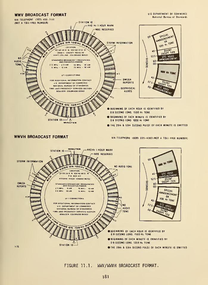
WWV BROADCAST FORMATVIA TELEPHONE 1303) 499-7111
[NOT A TOLL-FREE NUMBER}
US DEPARTMENT OF COMMERCENational Bureau of Standards
-STATION 10
-440 Hz 1 HOUR MARK
-NBS RESERVED
BEGINNING OF EACH HOUR IS IDENTIFIED BY
8 SECONO LONG. 1500 Hz TONE
BEGINNING OF EACH MINUTE IS IDENTIFIED BY
8 SECOND LONG. 1000 Hz TONE
THE 29th & 59th SECONO PULSE OF EACH MINUTE IS OMITTED
WWVH BROADCAST FORMAT VIA TELEPHONE {8081 335-4363 INOT A TOLL-FREE NUMBERI
MIIMUTISTATION ID , o
440 Hz 1 HOUR MARK
NBS RESERVEO
STORM INFORMATION
NO AUDIO TONE
1/75STATION 10
• BEGINNING OF EACH HOUR IS IDENTIFIED BY
8 SECOND LONG. 1500 Hz TONE
• BEGINNING OF EACH MINUTE IS IDENTIFIED BY
8 SECOND LONG. 1200 Hz TONE
• THE 29th & 59th SECONO PULSE OF EACH MINUTE IS OMITTED
FIGURE 11.1. WWV/WWVH BROADCAST FORMAT,
181
GLOSSARY
The following definitions are offered as an aid to the reader. However, they may notconform to the definitions as recommended by the CC1R or other appropriate organizations.Further, we have not attempted to include all possible unfamiliar terms. Many terms are fullyexplained in the text and have not been repeated here.
ACCURACY - how well something agrees with the definition or standard. In the case of frequency,an oscillator is said to be accurate if it agrees with the master oscillator at theNational Bureau of Standards in Boulder, Colorado. There is often confusion aboutthe definition of the terms resolution, precision, and accuracy.
AGING - the process whereby crystals change their characteristics. A quartz crystal of 100 kHzmay age until its frequency becomes 100.01 kHz. The process of aging is not well
understood.
AMBIGUITY - the properties of something that allows it to have more than one possible meaning.In the case of a clock, if it displays 3 hours, 5 minutes, it could be morning or night.The clock is then said to be ambiguous to the hour. Ambiguity is overcome in time codesby sending the day number. This makes that particular time code ambiguous to the year.
ANALOG FREQUENCY METERS - that class of instruments that uses needle movements rather thanlighted digits to indicate frequency. Accuracies obtained with these meters are oftenless than with their digital counterparts.
AT CUTS - one of the many ways in which bulk quartz material can be sliced to produce frequencycontrolling crystals. The AT cut is usually used for frequencies above 500 kHz andhas excellent frequency versus temperature characteristics.
ATOM DETECTION - a process used in atomic clocks to detect atoms.
ATOMIC TIME (TA) - the time obtained by counting cycles of an atomic clock as opposed to timebased on the earth's rotation. Atomic time is extremely uniform.
AUTOMATIC GAIN CONTROL (AGC) - a circuit used in communications receivers so that both weakand strong stations can be heard with nominally equal volume.
BALANCE WHEEL - a small wheel in watches under control of the hairspring. The oscillatingbalance wheel determines the rate of the watch.
BURST - the name given to a short signal consisting of a number of cycles. The WWV tick couldproperly be called a burst.
CALIBRATION - a frequency source can be calibrated by measuring its frequency difference withrespect to the National Bureau of Standards frequency standard. It is also possibleto calibrate one frequency source against another.
CESIUM STANDARD (Cs) - This term is often used to describe any oscillator that uses cesiumto obtain atomic resonance.
CHRONOMETER - a very accurate clock or watch, usually used on ships for navigation. Thisname has also been applied to digital instruments driven from quartz crystals.
CHU - the call letters of the Canadian broadcasting station at Ottawa, Canada, which broadcastsfrequency and time signals similar to those of WWV.
COLOR BAR COMPARATOR - an instrument that is used to compare a user's oscillator to the
television color subcarrier by putting a colored vertical bar on the television screen.
CYCLE CORRECTION - the correction applied to low frequency radio data that allows for the
chance that the receiver may be locked to the incorrect carrier cycle. In the caseof Loran-C, one cycle is 10 microseconds. For the WWV tone, one cycle would be
1 mi 1 1 i second.
183
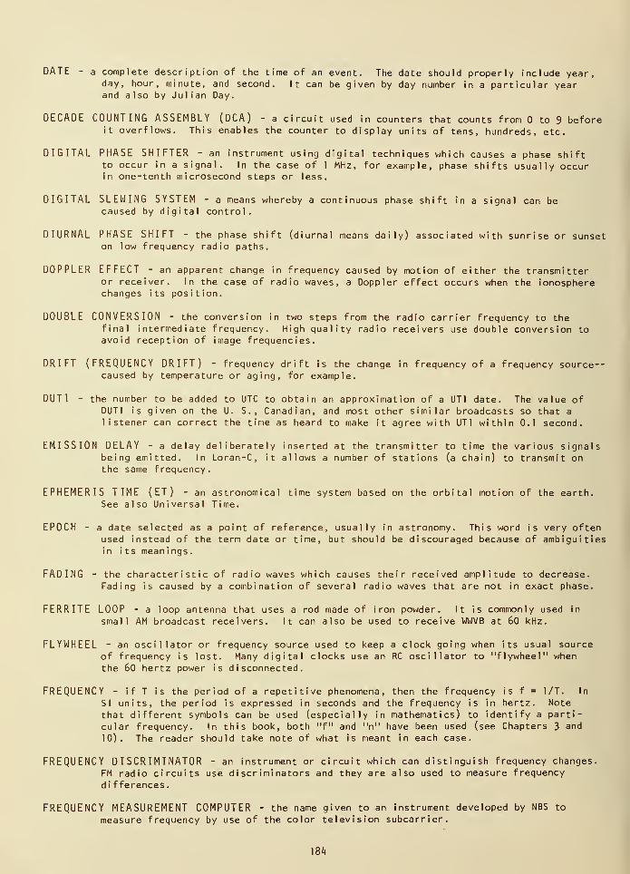
DATE - a complete description of the time of an event. The date should properly include year,day, hour, minute, and second. It can be given by day number in a particular yearand also by Julian Day.
DECADE COUNTING ASSEMBLY (DCA) - a circuit used in counters that counts from to 9 beforeit overflows. This enables the counter to display units of tens, hundreds, etc.
DIGITAL PHASE SHIFTER - an instrument using digital techniques which causes a phase shiftto occur in a signal. In the case of 1 MHz, for example, phase shifts usually occurin one-tenth microsecond steps or less.
DIGITAL SLEWING SYSTEM - a means whereby a continuous phase shift in a signal can becaused by digital control.
DIURNAL PHASE SHIFT - the phase shift (diurnal means daily) associated with sunrise or sunseton low frequency radio paths.
DOPPLER EFFECT - an apparent change in frequency caused by motion of either the transmitteror receiver. In the case of radio waves, a Doppler effect occurs when the ionospherechanges its position.
DOUBLE CONVERSION - the conversion in two steps from the radio carrier frequency to thefinal intermediate frequency. High quality radio receivers use double conversion toavoid reception of image frequencies.
DRIFT (FREQUENCY DRIFT) - frequency drift is the change in frequency of a frequency source-caused by temperature or aging, for example.
DUT1 - the number to be added to UTC to obtain an approximation of a UT1 date. The value ofDUT1 is given on the U. S., Canadian, and most other similar broadcasts so that a
listener can correct the time as heard to make it agree with UT1 within 0.1 second.
EMISSION DELAY - a delay deliberately inserted at the transmitter to time the various signalsbeing emitted. In Loran-C, it allows a number of stations (a chain) to transmit onthe same frequency.
EPHEMERIS TIME (ET) - an astronomical time system based on the orbital motion of the earth.See also Universal Time.
EPOCH - a date selected as a point of reference, usually in astronomy. This word is very oftenused instead of the term date or time, but should be discouraged because of ambiguitiesin its meanings.
FADING - the characteristic of radio waves which causes their received amplitude to decrease.Fading is caused by a combination of several radio waves that are not in exact phase.
FERRITE LOOP - a loop antenna that uses a rod made of iron powder. It is commonly used in
small AM broadcast receivers. It can also be used to receive WWVB at 60 kHz.
FLYWHEEL - an oscillator or frequency source used to keep a clock going when its usual sourceof frequency is lost. Many digital clocks use an RC oscillator to "flywheel" when
the 60 hertz power is disconnected.
FREQUENCY - if T is the period of a repetitive phenomena, then the frequency is f = 1/T. In
SI units, the period is expressed in seconds and the frequency is in hertz. Note
that different symbols can be used (especially in mathematics) to identify a parti-cular frequency. In this book, both "f" and "n" have been used (see Chapters 3 and
10). The reader should take note of what is meant in each case.
FREQUENCY DISCRIMINATOR - an instrument or circuit which can distinguish frequency changes.
FM radio circuits use discriminators and they are also used to measure frequency
di f ferences.
FREQUENCY MEASUREMENT COMPUTER - the name given to an instrument developed by NBS to
measure frequency by use of the color television subcarrier.
184
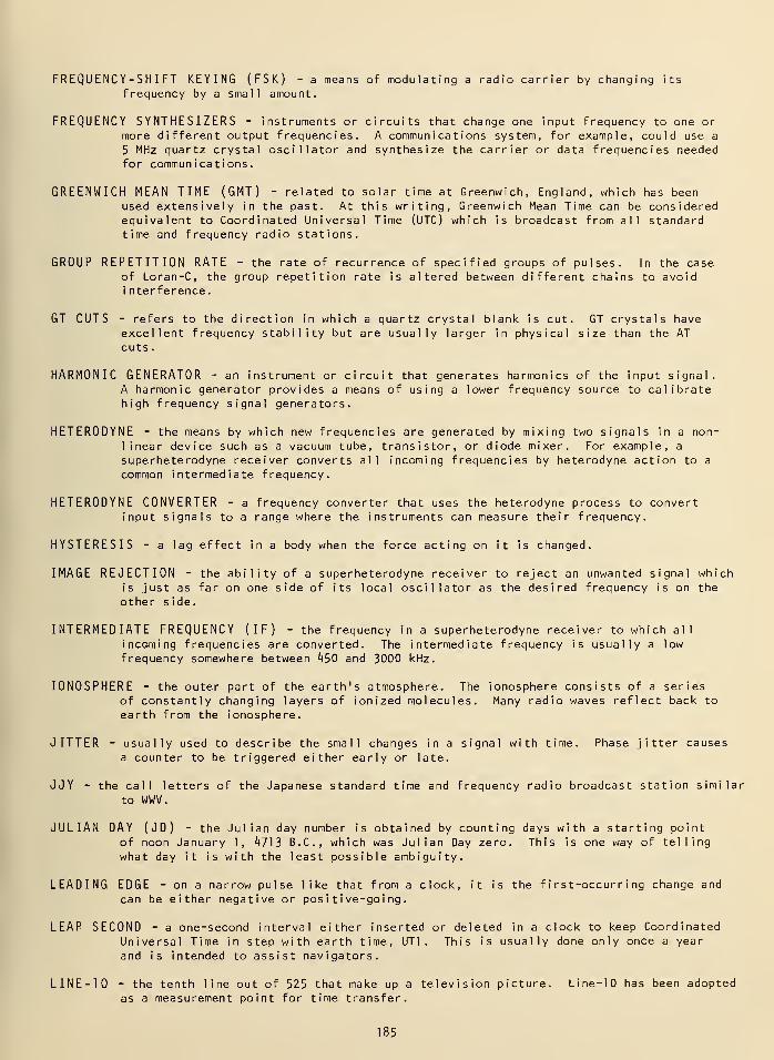
FREQUENCY-SHIFT KEYING (FSK) - a means of modulating a radio carrier by changing its
frequency by a small amount.
FREQUENCY SYNTHESIZERS - instruments or circuits that change one input frequency to one or
more different output frequencies. A communications system, for example, could use a
5 MHz quartz crystal oscillator and synthesize the carrier or data frequencies neededfor communications.
GREENWICH MEAN TIME (GMT) - related to solar time at Greenwich, England, which has been
used extensively in the past. At this writing, Greenwich Mean Time can be consideredequivalent to Coordinated Universal Time (UTC) which is broadcast from all standardtime and frequency radio stations.
GROUP REPETITION RATE - the rate of recurrence of specified groups of pulses. In the caseof Loran-C, the group repetition rate is altered between different chains to avoidi nterference.
GT CUTS - refers to the direction in which a quartz crystal blank is cut. GT crystals haveexcellent frequency stability but are usually larger in physical size than the AT
cuts
.
HARMONIC GENERATOR - an instrument or circuit that generates harmonics of the input signal.A harmonic generator provides a means of using a lower frequency source to calibratehigh frequency signal generators.
HETERODYNE - the means by which new frequencies are generated by mixing two signals in a non-
linear device such as a vacuum tube, transistor, or diode mixer. For example, a
superheterodyne receiver converts all incoming frequencies by heterodyne action to a
common intermediate frequency.
HETERODYNE CONVERTER - a frequency converter that uses the heterodyne process to convertinput signals to a range where the instruments can measure their frequency.
HYSTERESIS - a lag effect in a body when the force acting on it is changed.
IMAGE REJECTION - the ability of a superheterodyne receiver to reject an unwanted signal whichis just as far on one side of its local oscillator as the desired frequency is on the
other side.
INTERMEDIATE FREQUENCY (IF) - the frequency in a superheterodyne receiver to which all
incoming frequencies are converted. The intermediate frequency is usually a low
frequency somewhere between ^50 and 3000 kHz.
IONOSPHERE - the outer part of the earth's atmosphere. The ionosphere consists of a seriesof constantly changing layers of ionized molecules. Many radio waves reflect back to
earth from the ionosphere.
JITTER - usually used to describe the small changes in a signal with time. Phase jitter causesa counter to be triggered either early or late.
JJY - the call letters of the Japanese standard time and frequency radio broadcast station similar
to WWV.
JULIAN DAY (JD) - the Julian day number is obtained by counting days with a starting point
of noon January 1, ^713 B.C., which was Julian Day zero. This is one way of telling
what day it is with the least possible ambiguity.
LEADING EDGE - on a narrow pulse like that from a clock, it is the first-occurring change and
can be either negative or positive-going.
LEAP SECOND - a one-second interval either inserted or deleted in a clock to keep Coordinated
Universal Time in step with earth time, UT1 . This is usually done only once a year
and is intended to assist navigators.
LINE-10 - the tenth line out of 525 that make up a television picture. Line-10 has been adopted
as a measurement point for time transfer.
185
LISSAJOUS PATTERNS - the patterns obtained on a cathode ray tube by driving both the hori-zontal and vertical deflection plates with particular signals. Lissajous patternsare used for frequency calibration and phase measurement.
LONG-TERM STABILITY - describes the frequency change of an oscillator that occurs with time.Long-term usually refers to changes over times longer than 1 second.
LOOP ANTENNA - an antenna used for radio reception at many different frequencies. It consistsof a number of turns of wire usually in a shielded or pipe-type of enclosure. A loopantenna operates in the magnetic field of the signal and has a "figure-8" receptionpattern which enables it to null out undesired signals.
MASER (MICROWAVE AMPLIFICATION BY SIMULATED EMISSION OF RADIATION) - a device thatuses the natural oscillations of atoms and molecules to generate signals usually in
the microwave region.
MAXIMUM USABLE FREQUENCY (MUF) - the highest frequency that can be used for radio trans-missions without having the signal escape through the ionosphere. Signals below themaximum usable frequency will reflect off the ionosphere.
MEAN SOLAR TIME - time based on a mean solar day, which is the average length of all solardays in a solar year. The mean solar second is 1/86,^00 of a mean solar day.
MIXER - an electrical circuit that mixes two signals and produces a new signal that is usuallyeither the sum or the difference of the two inputs.
MODIFIED JULIAN DAY (MJD) - this is equal to the Julian date shifted so its origin occursat midnight on November 17, 1858. That is, it differs from the Julian Day by
2,^00,000.5 days exactly.
MULTIPATH - propagation of radio waves by more than one path from transmitter to receiver.This usually causes either fading or distortion.
NETWORK TELEVISION PROGRAM - any program that originates at either the East or West Coastnetworks of the U. S. broadcasters. It does not have to be a live program. It
simply has to start out at the network studios.
NULL DETECTOR - an instrument that is used to detect the absence of a signal. Null detectorsare usually more sensitive than peak detectors.
OFFSET (FREQUENCY) - frequency offset is the difference in the available frequency and the
nominal frequency. It is often deliberate. In the case of the U. S. televisionnetworks at this writing, the offset is about -3000 parts in 10^'. The term fre-
quency offset is used interchangeably with the terms relative or fractional
frequency.
OMEGA NAVIGATION SYSTEM - a low frequency (10 to 20 kHz) navigation system usually used in
the hyperbolic mode.
OPTICAL DETECTION - detection of signal or its properties by optical means.
OVERTONE CRYSTALS- crystals designed to operate at a frequency higher than their fundamental.
Crystal controlled oscillators as distinguished from crystal oscillators often use
overtone crystals.
PERIOD MEASUREMENT - a measurement of frequency by measuring the duration of the periods in
time units of the signal. Period measurements are always more accurate than
frequency measurements unless the frequency being measured is as high as the frequency
counter's time base. For example, a counter with a 1 MHz time base can be used in
the period mode for greater accuracy for frequencies up to 1 MHz.
PHASE DETECTOR - a circuit or instrument that detects the difference in phase (sometimes
in degrees or microseconds) between two signals. Phase detection is useful in
high resolution frequency detection.
186
PHASE ERROR MULTIPLIERS - a scheme whereby the difference in phase between two signals is
enhanced by multiplication and mixing techniques.
PHASE JUMP - the name given to sudden phase changes in a signal.
PHASE LOCK - a servo mechanism technique for causing one signal to follow another. They canbe but do not have to be at the same frequency. Phase locking in terms of frequencysources is analogous to a mechanical servo where one shaft or wheel follows another.
PHASE SIGNATURE - a deliberate phase offset to identify a signal. WWVB as broadcast is
deliberately phase shifted at 10 minutes after the hour. This aids the user by
letting him know that he really is tracking WWVB and not some other signal.
POWER LINE FREQUENCY - In the United States the power lines are held to a nominal 60 hertz.Variations in this of about + 50 ppm occur when the power system adjusts the frequencyto regulate power flow.
PORTABLE CLOCK - any clock which is designed to be transported. Usually it is an atomic clockwith suitable batteries.
PRECISION - the reproducibility of a given measurement. For example, a clock pulse could be
consistently measured to a precision of a few nanoseconds. Not to be confused withaccuracy. The same clock that is measured to a precision of a few nanoseconds couldbe in error by several seconds.
PRESCALING - the process whereby a frequency out of range of a measurement instrument can be
scaled down to within the range of that instrument.
PROPAGATION DELAY - the delay experienced by a signal as it traverses a radio path.
Q - the quality of a signal or detector or device. Q of coils is defined as the ratio of theinductive reactance to the resistance. It is also equal to the ratios of bandwidthof a resonator to its central frequency.
QUARTZ - a brilliant, crystalline mineral, mainly silicon dioxide.
RECEIVER DELAY - the delay experienced by the signal going from the antenna to the detector or
output device, speaker, or oscilloscope terminal. Typical receiver delays in highfrequency radio receivers are of the order of a few milliseconds.
REPRODUCIBILITY - the degree to which an oscillator will produce the same output frequencyfrom one time to another after it has been properly aligned.
RESOLUTION - the degree to which a measurement can be determined is called the resolution ofthe measurement. A time interval counter might only resolve tenths of seconds or a
few mi 1 1 i seconds.
RUBIDIUM (Rb) OSCILLATOR - an oscillator based on a resonance of rubidium gas.
SELECTIVITY - the ability of radio receiver circuits to separate one signal from another.
SENSITIVITY - the characteristic of a radio receiver that allows it to detect weak signals.
SHAPER - a circuit that provides uniform pulses from a variety of inputs. An example would be
a circuit to change sine waves into sharp pulses.
SHORT-TERM STABILITY - a description of the frequency fluctuations caused by random noisein an oscillator. To properly state the short-term stability, the number of samples,averaging time, repetition time, and system bandwidth must be specified.
SIDEREAL TIME (SIGH DEER 1 EEE AL) - time based on observations of stars rather than the
sun. Sidereal time is used by astronomers and a sidereal day is equal to about 23
hours, 56 minutes, and h seconds of solar time. Because it is based on observationsof stars, it is more accurately determined than solar time.
187
SIGNAL-TO-NOISE RATIO (SNR) - the ratio of the strength of a radio signal to that of the
noise. This is often a more useful term than simply signal strength.
SQUARING CIRCUIT - a circuit designed to produce square waves from an input waveform, quiteoften a sinusoid. This reduces the indecision about where zero crossings will occur.
STANDARD - a universally accepted reference. The NBS frequency standard is a cesium oscillatorlocated at the National Bureau of Standards in Boulder, Colorado. Many frequenciesgenerated and used in the United States are referenced to this standard.
STANDARD FREQUENCY BAND - radio bands allocated expressly for the purpose of distributingstandard frequency and/or time. For example, all of the transmissions of WWV occurin standard frequency bands centered on 2.5, 5, 10, and 15 MHz.
STATE SELECTION - the process whereby atoms or molecules are separated from atoms ormolecules in a different state.
SUBCARRIER - an additional signal inserted along with the main carrier in radio or televisiontransmission. The television color subcarrier is a signal added to the televisionformat at about 3.58 MHz from the main carrier.
SUNSPOTS - dark spots sometimes seen on the surface of the sun which are related to magneticand radio propagation disturbances on earth.
SUNSPOT CYCLES - cycles in the number of sunspots.
SYNCHRONIZATION - in the context of timing, synchronization means to bring two clocks or datastreams into phase so they agree. They need not be on time.
TCXO (TEMPERATURE COMPENSATED CRYSTAL OSCILLATOR) - a crystal oscillator that containsspecial components to minimize the effect of temperature on the crystal frequency.
TICK - an electrical signal, usually a pulse, designed for use in resetting of dividers, etc.
The WWV tick heard on its radio broadcast consists of 5 cycles of a 1 kHz sine wave.
TIME BASE - in a frequency counter that oscillator which provides the timing signals for meas-urement and control. The accuracy of the counter is directly related to the
time base.
TIME INTERVAL COUNTER - a counter designed to measure the time between events, zero
crossings for example.
TIME OF COINCIDENCE (LORAN) - that time when the Loran signal is coincident with an exact
second of Coordinated Universal Time. These times of coincidence will occur about
every 10 or 15 minutes and have been tabulated by the U. S. Naval Observatory.
TTL INTEGRATED CIRCUITS - a family of integrated circuits that uses transistor-transistorlogic. At this writing TTL has become the most popular family of integrated circuits
and is characterized by fast rise times. Unless deliberately modified, output levels
are nominally zero to 5 volts positive.
TRANSFER STANDARDS - the name given to a signal that is used to perform a calibration when
it can be referenced to a standard. An example would be the use of a VLF frequency
source to transfer frequency to a location based on its calibration at NBS.
TRIGGER ERROR - the error associated with false triggering caused by phase noise or jitter
on a signal .
UNIVERSAL TIME (UT) FAMILY - Universal Time is given in several ways. Apparent solar time
is first corrected by the equation of time to mean solar time, UTO. It is then again
corrected for migration of the earth's poles to obtain UT1 . This is further corrected
for periodicity of unknown origin to obtain UT2.
VFO - variable frequency oscillator as distinguished from a fixed frequency oscillator such as
a crystal
.
188
WAVE ANGLE - the angle above the surface of the earth at which a signal is transmitted from or
received by an antenna.
WAVEMETER - a meter for measuring frequency. Wavemeters usually work by having a coil that
collects part of the energy from a transmitter or a transmission line and displaysresonance on a meter movement.
ZERO BEAT - that condition between two signals when no beat is heard or seen between thesignals; that is, the frequencies are equal.
189
INDEX
AT CUT IN CRYSTALS 166
ACCURACY
ATOMIC RESONATORS 172
CALIBRATION
CHU 73Loran-C 150Televi s ion
Frequency 121,1 AO
Time 136,138,140
WWV/WWVH 73WWVB 105,107
CESIUM 174,178COUNTER 45DEFINITION 158
HYDROGEN MASER. ATOMIC 176,178QUARTZ CRYSTAL OSCILLATOR 167,178RUBIDIUM 175,178
ADJUSTABLE RATE DIVIDERS 70
AGING
QUARTZ CRYSTAL 10,45,166
ALGEBRA OF TIME AND FREQUENCY MEASUREMENTS 25
AMBIGUITY
PHASE CHART, WWVB 107+ 1 COUNT 34,45TELEVISION LINE-10 142
ANALOG FREQUENCY METER, DIRECT-READING 63
ANTENNAS
HF 77LF/VLF 105
TO REDUCE INTERFERENCE AT LF/VLF 112
WWV/WWVH, CHU 77WWVB 105
APPARENT SOLAR TIME 15
ASTRONOMICAL OBSERVATORIES 21
ASTRONOMICAL TIME 15
ASTRONOMY, USE OF TIME SCALES FOR 20
ATOMIC
BEAM, CESIUM 173
CLOCK
Cesium 173
World's First 16
191
FREQUENCY SOURCE 155-178HYDROGEN MASER I76OSCILLATORS 172
Cesium 173Rubidium 175Hydrogen 1 76
RESONATOR 172RUBIDIUM OSCILLATOR 175TIME (TA) 16
TIME SCALES (See TIME SCALES)
ATOMIC RESONANCE, ACHIEVING I69
AUTOMATIC TRANSFER OSCILLATOR 37
AVERAGE, SIGNAL 69
BIH (BUREAU INTERNATIONAL DE L'HEURE)
ROLE IN INTERNATIONAL COORDINATION OF TIME AND FREQUENCY 22
TIME SCALE, TA I (BIH) 16
BAND, RADIO FREQUENCY 9
BASE UNITS OF MEASUREMENT 3
BASIC STANDARDS 3
BEAM, CESIUM . 173
BEAT FREQUENCY METHOD 93
BROADCAST STATIONS (See RADIO BROADCASTS, Using for Calibration)
BULLETIN, NBS TIME AND FREQUENCY SERVICES
MONITORING DATA FOR TRACEABILITY TO NBS
Loran-C 1 16
NLK 116
Omega 1 16
Television
Color Subcarrier Frequency 125
Line-10 137
WWVB 116
BULLETIN, USNO TIME SERIES
MONITORING DATA FOR TRACEABILITY TO USNO
Loran-C 116
NAA/NLK 116
Omega 1 1 6
Television Line-10 1^2
BUREAU INTERNATIONAL DE L'HEURE (See BIH)
CGPM (GENERAL CONFERENCE ON WEIGHTS AND MEASURES) 16
CHU
ACCURACY, CALIBRATION 73
ANTENNAS 77
BROADCAST FORMAT 75
192
CALIBRATION TECHNIQUES
Frequency 92Time 81
CARRIER FREQUENCIES 75PROPAGATION PATH DELAY 99TIME CODE 13
TIME-OF-DAY ANNOUNCEMENTS 81
CABLE, DISTRIBUTION OF TIME AND FREQUENCY VIA 10
CALIBRATION
ACCURACY
HF Broadcasts (Time and Frequency ~lk
LF/VLF 107
Televi si on
Frequency 121,129,1^0Time \k0
DEFINITION 6
CALIBRATION TECHNIQUES
ELECTRONIC FREQUENCY COUNTER, USE OF 33FREQUENCY
CHU 92-99LF/VLF Broadcasts 112-116HF Broadcasts (WWV/WWVH, CHU)
Beat Frequency Method 93Oscilloscope Methods 95Time Comparison of Clocks 98
Television
Color Subcarrier 121-13**
Line-10 1 35~1 A3
WWV/WWVH 92-99WWVB 112-115
FREQUENCY COMPARISONS 52
OSCILLOSCOPE 50
PHASE LOCK 70
TIME
Loran-C 150
HF Broadcasts (WWV/WWVH, CHU) 81-88
WWV Time Code 89
Television Line-10 135-H3WWVB Time Code 116
CARRIER FREQUENCIES
CHU 75WWV/WWVH IkWWVB 105
LORAN-C 185
NAA, NLK, MSF 116
OMEGA 115
CATHODE-RAY OSCILLOSCOPE 50
CESIUM BEAM FREQUENCY OSCILLATORS 173
193
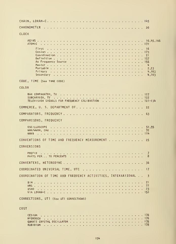
CHAIN, LORAN-C 1 45
CHRONOMETER 20
CLOCK
AGING 10,45 , 166
ATOMIC 172
First 16
Cesium 173Coordination 21
Definition 157As Frequency Source 156Master 4
Portable 2,23Primary 4,163Secondary 4,163
CODE, TIME (See TIME CODE)
COLOR
BAR COMPARATOR, TV 127
SUBCARRIER, TV 122
TELEVISION SIGNALS FOR FREQUENCY CALIBRATION 121-134
COMMERCE, U. S. DEPARTMENT OF 22
COMPARATORS, FREQUENCY 63
COMPARISONS, FREQUENCY
OSCILLOSCOPE 52,95WWV/WWVH, CHU 92
WWVB 114
CONVENTIONS OF TIME AND FREQUENCY MEASUREMENT 25
CONVERSIONS
PREFIX 7
PARTS PER... TO PERCENTS 8
CONVERTERS, HETERODYNE 36
COORDINATED UNIVERSAL TIME, UTC 17
COORDINATION OF TIME AND FREQUENCY ACTIVITIES, INTERNATIONAL . . 3
BIH 21
NBS 22
USNO 23
VIA LORAN-C 153
CORRECTIONS, UT1 (See UT1 CORRECTIONS)
COST
CESIUM 178
HYDROGEN 178
QUARTZ CRYSTAL OSCILLATOR 178
RUBIDIUM 178
194
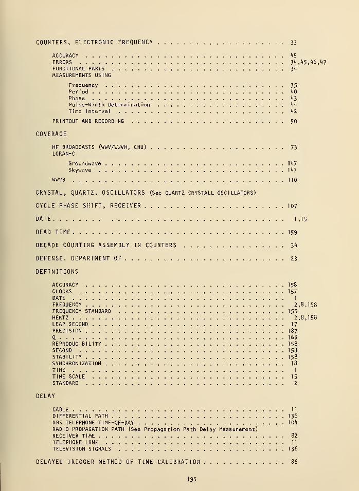
COUNTERS, ELECTRONIC FREQUENCY 33
ACCURACY 45
ERRORS 3^,^5,^6,47FUNCTIONAL PARTS 34
MEASUREMENTS USING
Frequency 35Period 40Phase 43Pulse-Width Determination 44
Time Interval 42
PRINTOUT AND RECORDING 50
COVERAGE
HF BROADCASTS (WWV/WWVH, CHU) 73LORAN-C
Groundwave , 147
Skywave 147
WWVB 110
CRYSTAL, QUARTZ, OSCILLATORS (See QUARTZ CRYSTALL OSCILLATORS)
CYCLE PHASE SHIFT, RECEIVER 107
DATE 1,15
DEAD TIME 159
DECADE COUNTING ASSEMBLY IN COUNTERS 34
DEFENSE. DEPARTMENT OF 23
DEFINITIONS
ACCURACY 158
CLOCKS 157
DATE 1
FREQUENCY 2,8,158FREQUENCY STANDARD 155HERTZ 2,8,158LEAP SECOND 17
PRECISION 187
Q 163REPRODUCIBILITY 158SECOND 158
STABILITY 158SYNCHRONIZATION 18
TIME 1
TIME SCALE 15
STANDARD 2
DELAY
CABLE 11
DIFFERENTIAL PATH 136
NBS TELEPHONE TIME-OF-DAY 104
RADIO PROPAGATION PATH (See Propagation Path Delay Measurement)RECEIVER TIME 82
TELEPHONE LINE 11
TELEVISION SIGNALS 136
DELAYED TRIGGER METHOD OF TIME CALIBRATION 86
195
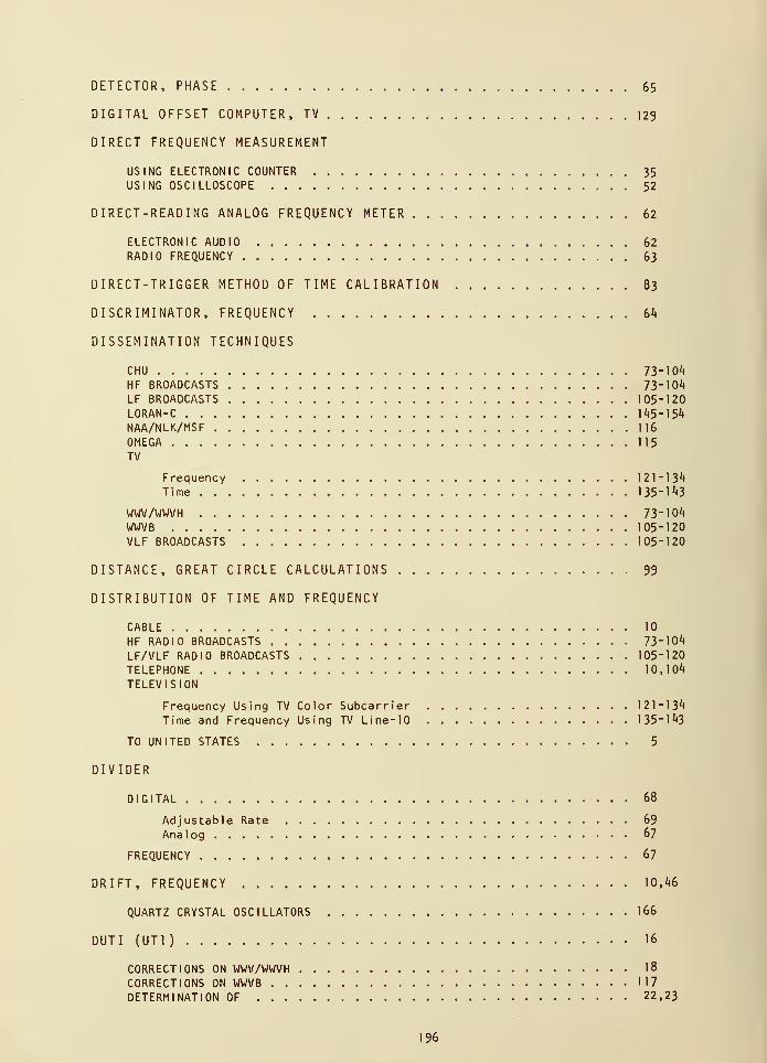
DETECTOR, PHASE 65
DIGITAL OFFSET COMPUTER, TV 129
DIRECT FREQUENCY MEASUREMENT
USING ELECTRONIC COUNTER 35USING OSCILLOSCOPE 52
DIRECT-READING ANALOG FREQUENCY METER 62
ELECTRONIC AUDIO 62RADIO FREQUENCY 63
DIRECT-TRIGGER METHOD OF TIME CALIBRATION 83
DISCRIMINATOR, FREQUENCY 64
DISSEMINATION TECHNIQUES
CHU 73-104HF BROADCASTS 73"104LF BROADCASTS 105-120LORAN-C 145-154NAA/NLK/MSF 116
OMEGA 115
TV
Frequency 121-134Time 135-143
WWV/WWVH 73-104WWVB 105-120
VLF BROADCASTS 105-120
DISTANCE, GREAT CIRCLE CALCULATIONS 99
DISTRIBUTION OF TIME AND FREQUENCY
CABLE 10
HF RADIO BROADCASTS 73"104
LF/VLF RADIO BROADCASTS 105-120
TELEPHONE 10,104
TELEVISION
Frequency Using TV Color Subcarrier 121-134
Time and Frequency Using TV Line-10 135-143
TO UNITED STATES 5
DIVIDER
DIGITAL 68
Adjustable Rate 69Analog 67
FREQUENCY 67
DRIFT, FREQUENCY 10,46
QUARTZ CRYSTAL OSCILLATORS 166
DUTI (UT1 )16
CORRECTIONS ON WWV/WWVH 18
CORRECTIONS ON WWVB 117
DETERMINATION OF 22,23
196
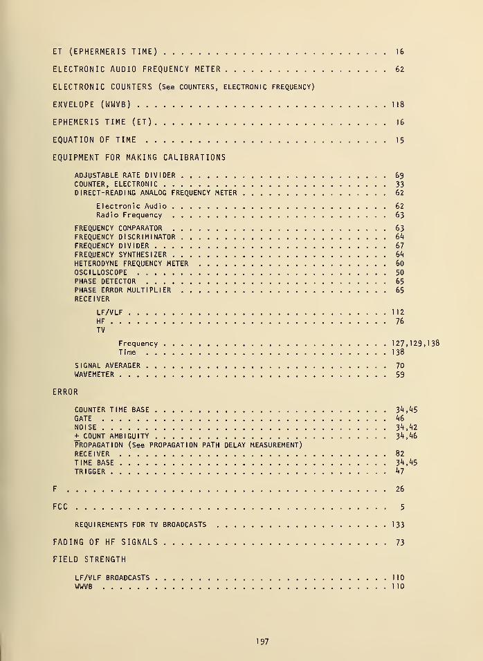
ET (EPHERMERIS TIME) 16
ELECTRONIC AUDIO FREQUENCY METER 62
ELECTRONIC COUNTERS (See COUNTERS, ELECTRONIC FREQUENCY)
ENVELOPE (WWVB) 118
EPHEMERIS TIME (ET) 16
EQUATION OF TIME 15
EQUIPMENT FOR MAKING CALIBRATIONS
ADJUSTABLE RATE DIVIDER 69
COUNTER, ELECTRONIC 33DIRECT-READING ANALOG FREQUENCY METER 62
Electronic Audio 62
Radio Frequency 63
FREQUENCY COMPARATOR 63FREQUENCY DISCRIMINATOR 64
FREQUENCY DIVIDER 67
FREQUENCY SYNTHESIZER 64
HETERODYNE FREQUENCY METER 60
OSCILLOSCOPE 50
PHASE DETECTOR 65PHASE ERROR MULTIPLIER 65
RECEIVER
LF/VLF 112
HF 76TV
Frequency 127,129,138Time 138
SIGNAL AVERAGER 70WAVEMETER 59
ERROR
COUNTER TIME BASE 34, 45GATE 46
NOISE 34,42+ COUNT AMBIGUITY 34,46PROPAGATION (See PROPAGATION PATH DELAY MEASUREMENT)RECEIVER 82
TIME BASE 34,45TRIGGER 47
F 26
FCC 5
REQUIREMENTS FOR TV BROADCASTS 133
FADING OF HF SIGNALS 73
FIELD STRENGTH
LF/VLF BROADCASTS 110
WWVB 110
197
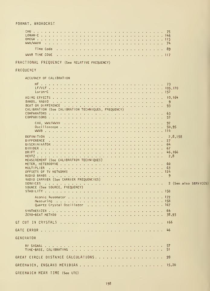
FORMAT, BROADCAST
CHU 75LORAN-C 146OMEGA 115WWV/WWVH 74
Time Code 89
WWVB TIME CODE 117
FRACTIONAL FREQUENCY (See RELATIVE FREQUENCY)
FREQUENCY
ACCURACY OF CALIBRATION
HF 73LF/VLF 105,120Loran-C 152
AGING EFFECTS 10,164
BANDS, RADIO 9
BEAT OR DIFFERENCE 93CALIBRATION (See CALIBRATION TECHNIQUES, FREQUENCY)COMPARATORS 63COMPARISONS 52
CHU, WWV/WWVH 92
Oscilloscope 50,95WWVB 114
DEFINITION 2,8,158DIFFERENCE 27DISCRIMINATOR 64
DIVIDER 67
DRIFT 46,166HERTZ 2,8MEASUREMENT (See CALIBRATION TECHNIQUES)METER, HETERODYNE 60
MULTIPLIER 63
OFFSETS OF TV NETWORKS 124
RADIO BANDS 9
RADIO CARRIER (See CARRIER FREQUENCIES)SERVICES 2 (See also SERVICES)SOURCE (See SOURCE, FREQUENCY)STABILITY 158
Atomic Resonator 172
Measuring 158
Quartz Crystal Oscillator 167
SYNTHESIZER 64
ZERO-BEAT METHOD 38,93
GT CUT IN CRYSTALS 166
GATE ERROR 46
GENERATOR
RF SIGNAL 57
TIME-BASE, CALIBRATING 51
GREAT CIRCLE DISTANCE CALCULATIONS 99
GREENWICH, ENGLAND MERIDIAN 15,20
GREENWICH MEAN TIME (See UTC)
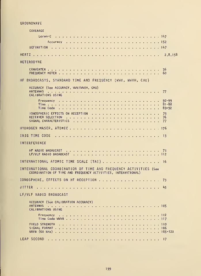
GROUNDWAVE
COVERAGE
Loran-C 1^7
Accuracy 152
DEFINITION 147
HERTZ 2,8,158
HETERODYNE
CONVERTER 36
FREQUENCY METER 60
HF BROADCASTS, STANDARD TIME AND FREQUENCY (WWV, WWVH, CHU)
ACCURACY (See ACCURACY, WWV/WWVH, CHU)
ANTENNAS 77CALIBRATIONS USING
Frequency 92-99Time 81-88Time Code 89-92
IONOSPHERIC EFFECTS ON RECEPTION 73RECEIVER SELECTION 76
SIGNAL CHARACTERISTICS 77
HYDROGEN MASER, ATOMIC 176
IRIG TIME CODE 13
INTERFERENCE
HF RADIO BROADCAST 73
LF/VLF RADIO BROADCAST 112
INTERNATIONAL ATOMIC TIME SCALE (TAI) 16
INTERNATIONAL COORDINATION OF TIME AND FREQUENCY ACTIVITIES (SeeCOORDINATION OF TIME AND FREQUENCY ACTIVITIES, INTERNATIONAL)
IONOSPHERE, EFFECTS ON HF RECEPTION 73
JITTER US
LF/VLF RADIO BROADCAST
ACCURACY (See CALIBRATION ACCURACY)ANTENNAS 105
CALIBRATIONS USING
Frequency 112
Time Code WWVB 117
FIELD STRENGTH 110
SIGNAL FORMAT 106
WWVB (60 kHz) 105-120
LEAP SECOND 17
199
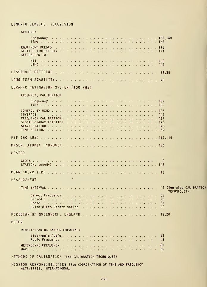
LINE-10 SERVICE, TELEVISION
ACCURACY
Frequency 136,140Time 1 36
EQUIPMENT NEEDED I38GETTING TIME-OF-DAY 1 42
REFERENCED TO
NBS 136USNO 1 42
LISSAJOUS PATTERNS 53,95
LONG-TERM STABILITY 46
LORAN-C NAVIGATION SYSTEM (100 kHz)
ACCURACY, CALIBRATION
Frequency 152Time 152
CONTROL BY USNO 145COVERAGE 147
FREQUENCY CALIBRATION 152
SIGNAL CHARACTERISTICS 148SLAVE STATION 146
TIME SETTING 150
MSF (60 kHz) 112,116
MASER, ATOMIC HYDROGEN 176
MASTER
CLOCK 4
STATION, LORAN-C 146
MEAN SOLAR TIME 15
MEASUREMENT
TIME INTERVAL 42 (See also CALIBRATIONTECHNIQUES)
Direct Frequency 35Period 40
Phase 43
Pulse-Width Determination 44
MERIDIAN OF GREENWICH, ENGLAND 15,20
METER
DIRECT-READING ANALOG FREQUENCY
Electronic Audio 62
Radio Frequency 63
HETERODYNE FREQUENCY 60
WAVE 59
METHODS OF CALIBRATION (See CALIBRATION TECHNIQUES)
MISSION RESPONSIBILITIES (See COORDINATION OF TIME AND FREQUENCY
ACTIVITIES, INTERNATIONAL)
200
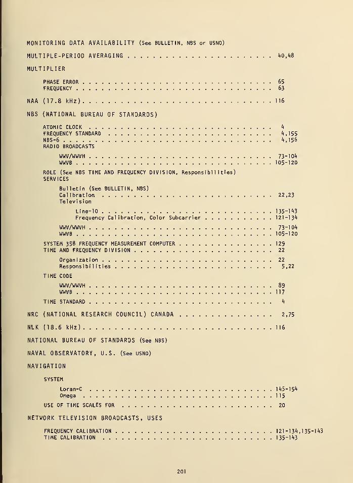
MONITORING DATA AVAILABILITY (See BULLETIN, NBS or USNO)
MULTIPLE-PERIOD AVERAGING 40,48
MULTIPLIER
PHASE ERROR 65
FREQUENCY 63
NAA (17.8 kHz) 116
NBS (NATIONAL BUREAU OF STANDARDS)
ATOMIC CLOCK 4
FREQUENCY STANDARD 4,155NBS-6 4,156RADIO BROADCASTS
WWV/WWVH 73-104WWVB 105-120
ROLE (See NBS TIME AND FREQUENCY DIVISION, Responsibilities)SERVICES
Bulletin (See BULLETIN, NBS)
Calibration 22,23Televi si on
Line-10 135-143
Frequency Calibration, Color Subcarrier 121-134
WWV/WWVH 73-104WWVB 105-120
SYSTEM 358 FREQUENCY MEASUREMENT COMPUTER 129TIME AND FREQUENCY DIVISION 22
Organization 22
Responsibilities 5,22
TIME CODE
WWV/WWVH 89WWVB 117
TIME STANDARD 4
NRC (NATIONAL RESEARCH COUNCIL) CANADA 2,75
NLK (18.6 kHz) 116
NATIONAL BUREAU OF STANDARDS (See NBS)
NAVAL OBSERVATORY, U.S. (See USNO)
NAVIGATION
SYSTEM
Loran-C 145-154Omega 115
USE OF TIME SCALES FOR 20
NETWORK TELEVISION BROADCASTS, USES
FREQUENCY CALIBRATION 121-134,135-143TIME CALIBRATION 135"l43
201
NOISE
ERRORS 34,32,42QUARTZ CRYSTAL OSCILLATOR 167
NULL DETECTORS 37
OBSERVATORIES, ASTRONOMICAL 21
OMEGA NAVIGATION SYSTEM
FORMAT 115
MONITORING DATA 116
ORGANIZATION OF TIME AND FREQUENCY ACTIVITIES, INTERNATIONAL (See
COORDINATION OF TIME AND FREQUENCY ACTIVITIES, INTERNATIONAL)
OSCILLATOR
ATOMIC 4,172AUDIO 57AUTOMATIC TRANSFER 37
CESIUM BEAM 173,178HYDROGEN MASER 176,178QUARTZ CRYSTAL (See QUARTZ CRYSTAL OSCILLATOR)RUBIDIUM 175,178TELEVISION NETWORK 122
TRANSFER
Automatic 37Phase-Locked 37
VARIABLE FREQUENCY (VFO) 37
OSCILLOSCOPE, CATHODE-RAY 50
OSCILLOSCOPE, METHODS OF CALIBRATION USING
DIRECT MEASUREMENT OF FREQUENCY 52
FREQUENCY COMPARISON 52
LISSAJOUS PATTERNS 53,95PHOTOGRAPHY 88
PATTERN DRIFT 97
SWEEP FREQUENCY CALIBRATION 58
TIME BASE, CALIBRATING 51
TIME INTERVAL 59
PTTI (PRECISE TIME AND TIME INTERVAL) 23
PATH DELAY, RADIO PROPAGATION (See PROPAGATION PATH DELAY MEASUREMENT)
PATTERN DRIFT METHOD OF CALIBRATION 97
PATTERNS, LISSAJOUS 53,95
PERIOD MEASUREMENT ^0
PHASE
CHANGES, WWVB, LF/VLF 106
DETECTOR 56,65
ERROR MULTIPLIER 56,65
INSTABILITY OF TV SIGNALS 123
JUMPS, TELEVISION 123
LOCK LOOP 71
LOCK TECHNIQUE 71
202
MEASUREMENT 43,122RECORDINGS FOR FREQUENCY CALIBRATION, WWVB 114RETARDATION, LF/VLF 106
SHIFT IDENTIFICATION, WWVB 113SHIFT
LF/VLF 106Cycle 107
TRACKING RECEIVER 71
PHOTOGRAPHY, OSCILLOSCOPE 88
PIEZOELECTRIC EFFECT 164
+ 1 COUNT AMBIGUITY 34,46
PORTABLE CLOCK 23
PRECISION, DEFINITION 1 87
PRESCALING 36
PRIMARY
CLOCK 4
FREQUENCY STANDARD 163
PRINTER-RECORDER 50
PROPAGATION
CHARACTERISTICS
HF 73LF/VLF 106
DIFFERENTIAL PATH DELAY 1 36
PATH DELAY MEASUREMENT
HF 83,99LF/VLF 107Time Code 14
PUBLICATIONS (See BULLETIN, NBS or USNO)
PULSE-WIDTH DETERMINATION MEASUREMENT 44
Q, RESONATOR
CESIUM 174DEFINITION 163HYDROGEN 176QUARTZ CRYSTAL 167REQUIREMENTS 64
RUBIDIUM 175
QUARTZ CRYSTAL OSCILLATOR
ACCURACY 167,178AGING 10,46,166CHARACTERISTICS 164
COST 168,178DRIFT 10,46,166FREQUENCY STABILITY 167
LONG-TERM DRIFT 46
PERFORMANCE 1 67PROPERTIES 164
Q 167
SHORT-TERM STABILITY 45
TEMPERATURE EFFECTS 1 66
203

RADIO ASTRONOMY OBSERVATORY 21
RADIO BROADCASTS (USING FOR CALIBRATION)
CHU 73-104FORMAT 74HF 73"104LF/VLF 105-120LORAN-C 145-154NAA, NLK, MSF 116
NBS 73-104,105-120OMEGA 115U. S. NAVY 105-120WWV/WWVH 73-104WWVB 105-120
RADIO FREQUENCY
BAND 9
METER 63
RADIO PROPAGATION DELAY MEASUREMENT (See PROPAGATION PATH DELAY MEASUREMENT)
RECEIVER
CYCLE PHASE SHIFT, LF/VLF 107
DELAY 14,82SELECTION (HF) 76
TIME DELAY MEASUREMENTS 82
RELATIVE FREQUENCY
DIFFERENCE 5'27
F 26
REPRODUCIBILITY 158
RESONANCE
ATOMIC 168
DETECTING 169
RESONATOR
ATOMIC
Accuracy 172
Detecting Resonance 169
Stability 172
State Selection 168
QUARTZ CRYSTAL 164
RESPONSIBILITIES IN TIME AND FREQUENCY COORDINATION (See COORDINATIONOF TIME AND FREQUENCY ACTIVITIES, INTERNATIONAL)
RUBIDIUM GAS CELL OSCILLATOR 175
S, RELATIVE FREQUENCY DIFFERENCE 27
SCALE, TIME (See TIME SCALE)
SCHMITT TRIGGER 48
SECOND
DEFINITION 158
LEAP 17
204
NBS
SECONDARY
CLOCK 4
FREQUENCY STANDARD 1 63
SECONDS TICK, WWV/WWVH 81
SERVICES
BULLETIN
NBS Time and Frequency Services (See BULLETIN, NBS)USNO Time Series (See BULLETIN, USNO)
Telephone Time-of-Day 104
Televi si on
Frequency Calibration, Color Subcarrier 121-13**
Time and Frequency Calibration, Line-10 135-143
Time and Frequency Division 22WWV/WWVH 73-10**
WWVB 105-120
RADIO BROADCAST
CHU 73-10**
HF 73-10**
LF/VLF 105-120Loran-C 145-15**
NAA, NLK, MSF 116
Omega 115
USNO 23
SHIFT, DIURNAL, LF/VLF 106
SHORT-TERM STABILITY 45
SIDEREAL TIME 15
SIGNAL
AVERAGER 71
CHARACTERISTICS
HF 77LF/VLF 106
Loran-C 148Television 123WWV/WWVH 77WWVB 106
FORMAT
CHU 75Loran-C 145
Omega 115
WWV/WWVH 74WWVB 106
SKYWAVE
COVERAGE, LORAN-C 147
Accuracy 154
DEFINITION 147HOPS, HF 100
205
SLAVE STATION, LORAN-C 146
SOLAR TIME 15
SOURCE, FREQUENCY
ATOMIC OSCILLATOR
Cesium Beam 1 73Hydrogen Maser 1 76
Rubidium 175
COMPARISONS OF 178PERFORMANCE 158PRIMARY AND SECONDARY STANDARDS 1 63QUARTZ CRYSTAL OSCILLATOR 164
RESONATORS 161
STABILITY (See STABILITY)
SPECIFICATIONS, STABILITY 45
STABILITY
ATOMIC OSCILLATOR
Cesium Beam 174,178Hydrogen Maser 176,178Rubidium 175,178
DEFINITION 153FRACTIONAL FREQUENCY 159QUARTZ CRYSTAL OSCILLATOR 163
SPECIFICATIONS
Long-Term 46
Short-Term 45
TELEVISION COLOR SUBCARRIER 133
STANDARDS
ATOMIC 4
BASIC 3
CESIUM BEAM 173DEFINITION 2,155FREQUENCY 4
HYDROGEN MASER 176NBS TIME AND FREQUENCY 4
PRIMARY (DEFINED) 163
RUBIDIUM 175SECONDARY (DEFINED) 163
STATE SELECTION, ATOMIC 168
STATE STANDARDS LABS 5
SUBCARRIER, COLOR TELEVISION, 3.58 MHz 122
SUNDIAL 15
SWEEP FREQUENCY CALIBRATION 58
SYNTHESIZER, FREQUENCY 64
SYNCHRONIZATION, SYSTEMS 18
TA (ATOMIC TIME) 16
TAI (INTERNATIONAL ATOMIC TIME) 16
206
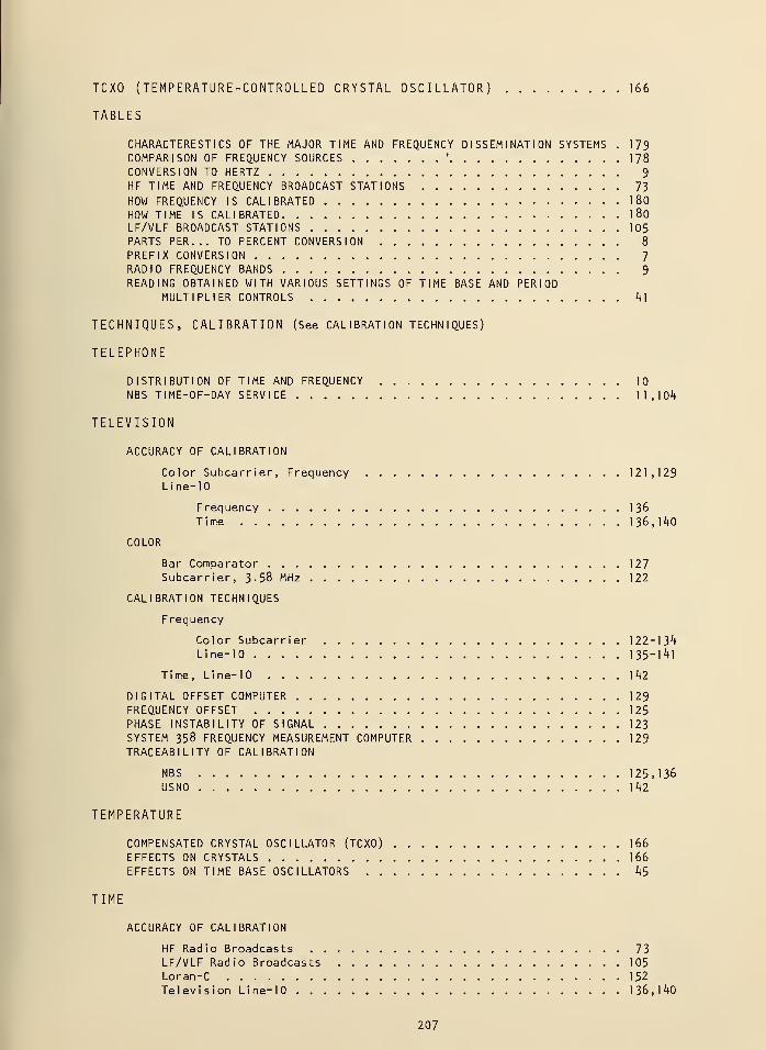
TCXO (TEMPERATURE-CONTROLLED CRYSTAL OSCILLATOR) 166
TABLES
CHARACTERESTICS OF THE MAJOR TIME AND FREQUENCY DISSEMINATION SYSTEMS . 179COMPARISON OF FREQUENCY SOURCES '
178CONVERSION TO HERTZ 9
HF TIME AND FREQUENCY BROADCAST STATIONS 73
HOW FREQUENCY IS CALIBRATED 180
HOW TIME IS CALIBRATED 1 80LF/VLF BROADCAST STATIONS 105PARTS PER... TO PERCENT CONVERSION 8
PREFIX CONVERSION 7RADIO FREQUENCY BANDS 9READING OBTAINED WITH VARIOUS SETTINGS OF TIME BASE AND PERIOD
MULTIPLIER CONTROLS 41
TECHNIQUES, CALIBRATION (See CALIBRATION TECHNIQUES)
TELEPHONE
DISTRIBUTION OF TIME AND FREQUENCY 10
NBS TIME-OF-DAY SERVICE 11,1 O^t
TELEVISION
ACCURACY OF CALIBRATION
Color Subcarrier, Frequency 121,129Line-10
Frequency 136
Time 136,140
COLOR
Bar Comparator 127Subcarrier, 3-58 MHz 122
CALIBRATION TECHNIQUES
Frequency
Color Subcarrier 122-134Line-10 135- Hi
Time, Line-10 1 42
DIGITAL OFFSET COMPUTER 129FREQUENCY OFFSET 125
PHASE INSTABILITY OF SIGNAL 123SYSTEM 358 FREQUENCY MEASUREMENT COMPUTER 129
TRACEABILITY OF CALIBRATION
NBS 125,136USNO 142
TEMPERATURE
COMPENSATED CRYSTAL OSCILLATOR (TCXO) 166
EFFECTS ON CRYSTALS 166
EFFECTS ON TIME BASE OSCILLATORS 45
TIME
ACCURACY OF CALIBRATION
HF Radio Broadcasts 73LF/VLF Radio Broadcasts 105
Loran-C 152
Television Line-10 136,140
207
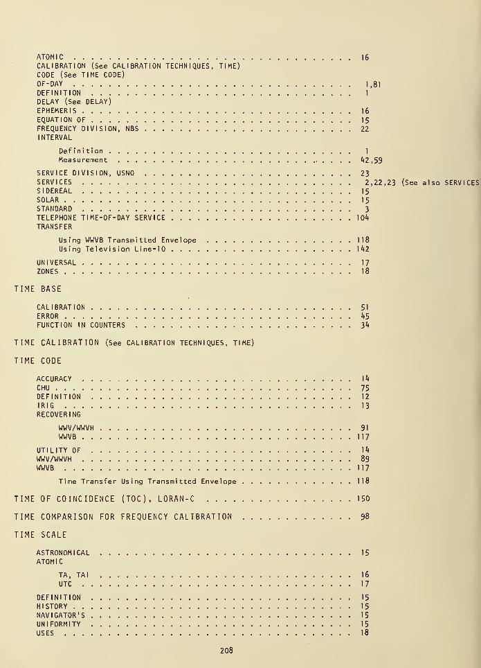
ATOMIC 16
CALIBRATION (See CALIBRATION TECHNIQUES, TIME)
CODE (See TIME CODE)
OF-DAY 1,81
DEFINITION 1
DELAY (See DELAY)EPHEMERIS 16
EQUATION OF 15
FREQUENCY DIVISION, NBS 22
INTERVAL
Definition 1
Measurement *»2,59
SERVICE DIVISION, USNO 23SERVICES 2,22,23 (See also SERVICES]SIDEREAL 15
SOLAR 15
STANDARD 3
TELEPHONE TIME-OF-DAY SERVICE 10*4
TRANSFER
Using WWVB Transmitted Envelope 118
Using Television Line-10 142
UNIVERSAL 17
ZONES 18
TIME BASE
CALIBRATION 51
ERROR k5
FUNCTION IN COUNTERS }>k
TIME CALIBRATION (See CALIBRATION TECHNIQUES, TIME)
TIME CODE
ACCURACY \k
CHU 75
DEFINITION 12
IRIG 13
RECOVERING
WWV/WWVH 91
WWVB 117
UTILITY OF \k
WWV/WWVH 89WWVB 117
Time Transfer Using Transmitted Envelope 118
TIME OF COINCIDENCE (TOC), LORAN-C 150
TIME COMPARISON FOR FREQUENCY CALIBRATION 98
TIME SCALE
ASTRONOMICAL 15
ATOMIC
TA, TAI 16
UTC 17
DEFINITION 15
HISTORY 15
NAVIGATOR'S 15
UNIFORMITY 15
USES 18
208
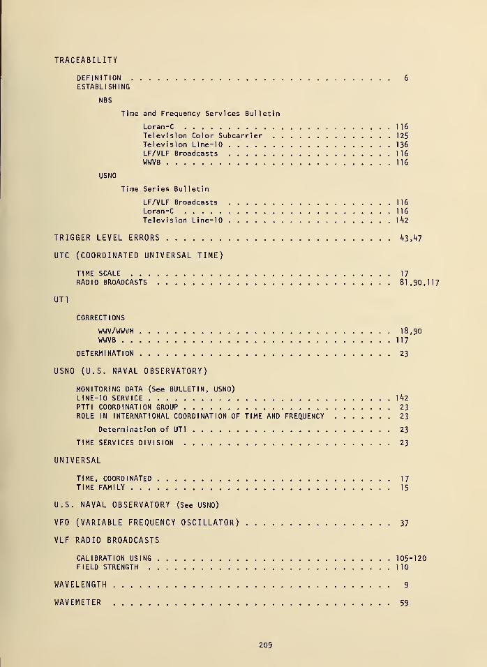
TRACEABILITY
DEFINITION 6
ESTABLISHING
NBS
Time and Frequency Services Bulletin
Loran-C 116
Television Color Subcarrier 125
Television Line- 10 136
LF/VLF Broadcasts 116WWVB 116
USNO
Time Series Bulletin
LF/VLF Broadcasts 116Loran-C 116
Television Line- 10 ]k2
TRIGGER LEVEL ERRORS ^3,^7
UTC (COORDINATED UNIVERSAL TIME)
TIME SCALE 17
RADIO BROADCASTS 81,90,117
UT1
CORRECTIONS
WWV/WWVH 18,90WWVB 117
DETERMINATION . 23
USNO (U.S. NAVAL OBSERVATORY)
MONITORING DATA (See BULLETIN, USNO)LINE-10 SERVICE 142
PTTI COORDINATION GROUP 23ROLE IN INTERNATIONAL COORDINATION OF TIME AND FREQUENCY 23
Determination of UT1 23
TIME SERVICES DIVISION 23
UNIVERSAL
TIME, COORDINATED 17
TIME FAMILY 15
U.S. NAVAL OBSERVATORY (See USNO)
VFO (VARIABLE FREQUENCY OSCILLATOR) 37
VLF RADIO BROADCASTS
CALIBRATION USING 105-120FIELD STRENGTH 110
WAVELENGTH 9
WAVEMETER 59
209
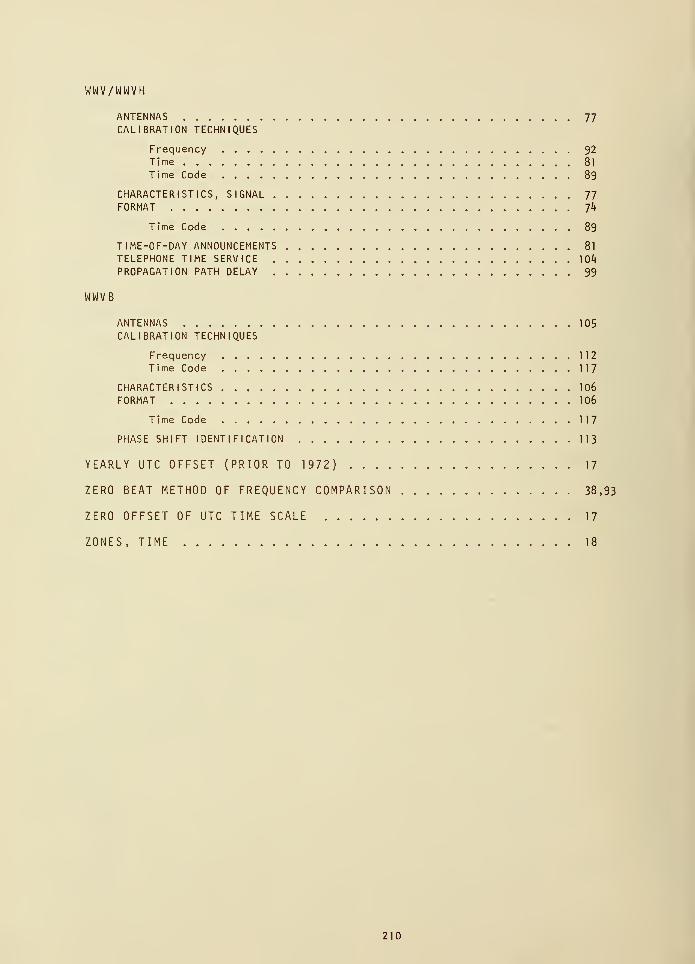
WWV/WWVH
ANTENNAS 77CALIBRATION TECHNIQUES
Frequency 92Time 8l
Time Code 89
CHARACTERISTICS, SIGNAL 77FORMAT 7k
Time Code 89
TIME-OF-DAY ANNOUNCEMENTS 81
TELEPHONE TIME SERVICE \0kPROPAGATION PATH DELAY 99
WWVB
ANTENNAS 105
CALIBRATION TECHNIQUES
Frequency 112
Time Code 117
CHARACTERISTICS 106
FORMAT 106
Time Code 117
PHASE SHIFT IDENTIFICATION 113
YEARLY UTC OFFSET (PRIOR TO 1972) 17
ZERO BEAT METHOD OF FREQUENCY COMPARISON 38,93
ZERO OFFSET OF UTC TIME SCALE 17
ZONES, TIME 18
210
NBS-114A (REV. 7-73)
U.S. DEPT. OF COMM.BIBLIOGRAPHIC DATA
SHEET
1. PUBLICATION OR REPORT NO.
NBS-TN-695
2. Gov't AccessionNo.
3. Recipient's Accession No.
4. TITLE AND SUBTITLE 5. Publication Date
May 1977
TIME AND FREQUENCY USERS 1 MANUAL 6. Performing Organization Code
277.067. AUTHOR(S)
George Kamas, editor8. Performing Organ. Report No.
9. PERFORMING ORGANIZATION NAME AND ADDRESS
NATIONAL BUREAU OF STANDARDSDEPARTMENT OF COMMERCEWASHINGTON, D.C. 20234
10. Project/Task/Work Unit No.
277621711. Contract/Grant No.
EIIIM-6
12. Sponsoring Organization Name and Complete Address (Street, City, State, ZIP)
Same as 9.
13. Type of Report & PeriodCovered
FINAL14. Sponsoring Agency Code
15. SUPPLEMENTARY NOTES
16. ABSTRACT (A 200-word or less factual summary of most significant information. If document includes a significant
bibliography or literature survey, mention it here.)
This manual has been written for the person who needs information
on making time and frequency measurements. It has been written at a
level that will satisfy those with a casual interest as well as labora-
tory engineers and technicians who use time and frequency every day.
It gives a brief history of time and frequency, discusses the roles
of the National Bureau of Standards and the U. S. Naval Observatory,
and explains how time and frequency are internationally coordinated.
It also explains what time and frequency services are available and
how to use them. It discusses the accuracy that can be achieved using
the different services as well as the pros and cons of using various
calibration methods.
17. KEY WORDS (six to twelve entries; alphabetical order; capitalize only the first letter of the first key word unless a proper
name; separated by semicolons)
Frequency calibration; high frequency; Loran-C; low frequency; radio broadcasts;standard frequencies ;- television color subcarrier; time and frequency calibrationmethods; time calibration; time signals.
18. AVAILABILITY Unlimited
IFor Official Distribution. Do Not Release to NTIS
| y j
Order From Sup. of Doc, U.S. Government Printing OfficeWashington, D.C. 20402, SD Cat. No. C13.46 :695
I !
Order From National Technical Information Service (NTIS)Springfield, Virginia 22151
19. SECURITY CLASS(THIS REPORT)
UNCLASSIFIED
20. SECURITY CLASS(THIS PAGE)
UNCLASSIFIED
21. NO. OF PAGES
217
22. Price
$2.80USCOMM-DC 29042-P74
•frU.S. Government Printing Office: 19 7 7-77 7-045/1243 Region 8
NBS TECHNICAL PUBLICATIONS
PERIODICALS
JOURNAL OF RESEARCH reports National Bureauof Standards research and development in physics,
mathematics, and chemistry. It is published in twosections, available separately:
• Physics and Chemistry (Section A)Papers of interest primarily to scientists working in
these fields. This section covers a broad range of physi-
cal and chemical research, with major emphasis onstandards of physical measurement, fundamental con-stants, and properties of matter. Issued six times a year.
A.nnual subscription: Domestic, $17.00; Foreign, $21.25.
• Mathematical Sciences (Section B)Studies and compilations designed mainly for the math-ematician and theoretical physicist. Topics in mathemat-ical statistics, theory of experiment design, numericalanalysis, theoretical physics and chemistry, logical de-
sign and programming of computers and computer sys-
tems. Short numerical tables. Issued quarterly. Annualsubscription: Domestic, $9.00; Foreign, $11.25.
DIMENSIONS/NBS (formerly Technical News Bulle-
tin)—This monthly magazine is published to informscientists, engineers, businessmen, industry, teachers,
students, and consumers of the latest advances in
science and technology, with primary emphasis on thework at NBS. The magazine highlights and reviewssuch issues as energy research, fire protection, building
technology, metric conversion, pollution abatement,health and safety, and consumer product performance.In addition, it reports the results of Bureau programsin measurement standards and techniques, properties of
matter and materials, engineering standards and serv-
ices, instrumentation, and automatic data processing.
Annual subscription : Domestic, $12.50; Foreign, $15.65.
N0NPERI0DICALS
Monographs—Major contributions to the technical liter-
ature on various subjects related to the Bureau's scien-
tific and technical activities.
Handbooks—Recommended codes of engineering andindustrial practice (including safety codes) developed
in cooperation with interested industries, professional
organizations, and regulatory bodies.
Special Publications—Include proceedings of conferencessponsored by NBS, NBS annual reports, and other
special publications appropriate to this grouping suchas wall charts, pocket cards, and bibliographies.
Applied Mathematics Series—Mathematical tables, man-uals, and studies of special interest to physicists, engi-
neers, chemists, biologists, mathematicians, com-puter programmers, and others engaged in scientific
and technical work.
National Standard Reference Data Series—Providesquantitative data on the physical and chemical proper-
ties of materials, compiled from the world's literature
and critically evaluated. Developed under a world-wideprogram coordinated by NBS. Program under authorityof National Standard Data Act (Public Law 90-396).
NOTE: At present the principal publication outlet for
these data is the Journal of Physical and ChemicalReference Data (JPCRD) published quarterly for NBSby the American Chemical Society (ACS) and the Amer-ican Institute of Physics (AIP). Subscriptions, reprints,
and supplements available from ACS, 1155 Sixteenth
St. N.W., Wash. D. C. 20056.
Building Science Series—Disseminates technical infor-
mation developed at the Bureau on building materials,
components, systems, and whole structures. The series
presents research results, test methods, and perform-ance criteria related to the structural and environmentalfunctions and the durability and safety characteristics
of building elements and systems.
Technical Notes—Studies or reports which are completein themselves but restrictive in their treatment of a
subject. Analogous to monographs but not so compre-hensive in scope or definitive in treatment of the sub-
ject area. Often serve as a vehicle for final reports of
work performed at NBS under the sponsorship of othergovernment agencies.
Voluntary Product Standards—Developed under proce-
dures published by the Department of Commerce in Part10, Title 15, of the Code of Federal Regulations. Thepurpose of the standards is to establish nationally rec-
ognized requirements for products, and to provide all
concerned interests with a basis for common under-
standing of the characteristics of the products. NBSadministers this program as a supplement to the activi-
ties of the private sector standardizing organizations.
Consumer Information Series—Practical information,
based on NBS research and experience, covering areas
of interest to the consumer. Easily understandable lang-
uage and illustrations provide useful background knowl-edge for shopping in today's technological marketplace.
Order above NBS publications from: Superintendentof Documents, Government Printing Office, Washington,D.C. 20402.
Order following NBS publications—NBSIR's and FIPSfrom the National Technical Information Services,
Springfield, Va. 22161.
Federal Information Processing Standards Publications
(FIPS PUBS)—Publications in this series collectively
constitute the Federal Information Processing Stand-ards Register. Register serves as the official source of
information in the Federal Government regarding stand-
ards issued by NBS pursuant to the Federal Propertyand Administrative Services Act of 1949 as amended,Public Law 89-306 (79 Stat. 1127), and as implementedby Executive Order 11717 (38 FR 12315, dated May 11,
1973) and Part 6 of Title 15 CFR (Code of FederalRegulations).
NBS Interagency Reports (NBSIR)—A special series of
interim or final reports on work performed by NBS for
outside sponsors (both government and non-govern-
ment). In general, initial distribution is handled by the
sponsor; public distribution is by the National Techni-
cal Information Services (Springfield, Va. 22161) in
paper copy or microfiche form.
BIBLIOGRAPHIC SUBSCRIPTION SERVICES
The following current-awareness and literature-survey
bibliographies are issued periodically by the Bureau:Cryogenic Data Center Current Awareness Service. A
literature survey issued biweekly. Annual subscrip-
tion: Domestic, $20.00; Foreign, $25.00.
Liquified Natural Gas. A literature survey issued quar-
terly. Annual subscription: $20.00.
Superconducting Devices and Materials. A literature
survey issued quarterly. Annual subscription: $20.00.
Send subscription orders and remittances for the pre-
ceding bibliographic services to National Bureau of
Standards, Cryogenic Data Center (275.02) Boulder,
Colorado 80302.
U.S. DEPARTMENT OF COMMERCENational Bureau of StandardsWashington, D.C. S0S34
OFFICIAL BUSINESS
Penalty for Private Use, $300
POSTAGE AND FEES PAIDU.S. DEPARTMENT OF COMMERCE
COM-215
SPECIAL FOURTH-CLASS RATE
.
BOOK