Embed Size (px)
Citation preview

Time-reversed absorbing condition: application to inverse problems
This article has been downloaded from IOPscience. Please scroll down to see the full text article.
2011 Inverse Problems 27 065003
(http://iopscience.iop.org/0266-5611/27/6/065003)
Download details:
IP Address: 132.66.7.211
The article was downloaded on 13/05/2011 at 13:08
Please note that terms and conditions apply.
View the table of contents for this issue, or go to the journal homepage for more
Home Search Collections Journals About Contact us My IOPscience

IOP PUBLISHING INVERSE PROBLEMS
Inverse Problems 27 (2011) 065003 (18pp) doi:10.1088/0266-5611/27/6/065003
Time-reversed absorbing condition: application toinverse problems
F Assous1, M Kray2, F Nataf2 and E Turkel3
1 Bar-Ilan University, 52900 Ramat-Gan & Ariel University Center, 40700 Ariel, Israel2 UPMC Universite Paris-06, UMR 7598, Laboratoire J L Lions, F-75006 Paris, France3 Department of Mathematics, Tel-Aviv University, 69978 Ramat Aviv, Israel
E-mail: [email protected], [email protected], [email protected] [email protected]
Received 20 October 2010, in final form 28 February 2011Published 10 May 2011Online at stacks.iop.org/IP/27/065003
AbstractThe aim of this paper is to introduce time-reversed absorbing conditions in time-reversal methods. They enable one to ‘recreate the past’ without knowing thesource which has emitted the signals that are back-propagated. We present twoapplications in inverse problems: the reduction of the size of the computationaldomain and the determination, from boundary measurements, of the locationand volume of an unknown inclusion. The method does not rely on any a prioriknowledge of the physical properties of the inclusion. Numerical tests withthe wave and Helmholtz equations illustrate the efficiency of the method. Thistechnique is fairly insensitive to noise in the data.
(Some figures in this article are in colour only in the electronic version)
1. Introduction
Since the seminal paper by Fink et al [16], time reversal is a subject of very active research.The main idea is to take advantage of the reversibility of wave propagation phenomena,for example in acoustics or electromagnetism in a non-dissipative but unknown medium, toback-propagate signals to the sources that emitted them. The initial experiment, see [16],was to refocus, very precisely, a recorded signal after passing through a barrier consisting ofrandomly distributed metal rods. The remarkable feature of this experiment is the practicalpossibility to precisely focus a signal after it has crossed random barriers. There have beennumerous applications of this physical principle, see [15], [19] and references therein. Thefirst mathematical analysis can be found in [3] for a homogeneous medium and in [9] and [8]for a random medium. In this study we do not consider random or inhomogenous media.
We will introduce a new method that enables one to ‘recreate the past’ without knowingthe source which has emitted the signals that will be back-propagated. This is made possible
0266-5611/11/065003+18$33.00 © 2011 IOP Publishing Ltd Printed in the UK & the USA 1

Inverse Problems 27 (2011) 065003 F Assous et al
by using time-reversed absorbing conditions (TRAC) after removing a small region enclosingthe source. This technique has at least two applications in inverse problems:
(i) the reduction of the size of the computational domain by redefining the reference surfaceon which the receivers appear to be located;
(ii) the location of an unknown inclusion from boundary measurements.
The first application is reminiscent of the redatuming method introduced in [7]. In ourcase, we use the wave equation and not a paraxial or parabolic approximation to it. This extendsthe domain of validity of the redatuming approach. Concerning the second application thereis a huge literature that deals with this inverse problem. We mention the MUSIC algorithm[25] and its application to imaging [20], the sampling methods first introduced in [11], seethe review paper [10] and references therein, and the DORT method [23]. Mathematicalanalysis of this kind of approach can be found in [12]. These methods were developed in thetime-harmonic domain for impenetrable inclusions. The TRAC method is designed in boththe time-dependent and harmonic domains and does not rely on any a priori knowledge of thephysical properties of the inclusion. It works both for impenetrable and penetrable inclusions.
The outline of the paper is as follows. In sections 2.1 and 2.2 we introduce the principle ofthe TRAC method both in the time-dependent and harmonic domains. We present in section 2.3two applications of the method in the context of inverse problems. The end of section 2 isdevoted to the explicit derivation of the method to the wave and Maxwell equations in boththe time-dependent and harmonic cases. In section 3 we give numerical applications of theTRAC method for the wave equation and the Helmholtz equation. We propose various criteriafor applying our method to inverse problems. We investigate the sensitivity with respect tothe magnitude of the noise in the data and its ability to handle penetrable inclusions.
2. The TRAC method and applications
2.1. The TRAC method in the time-dependent case
We consider an incident wave UI impinging on an inclusion D characterized by differentphysical properties from the surrounding medium. We denote by ∂D the boundary of thisinclusion. The total field UT can be decomposed into the incident and scattered field, soUT := UI + US . We consider the problem in d dimensions d = 1, 2, 3 and assume that thetotal field satisfies a linear hyperbolic equation (or system of equations) denoted by L, thatcan be written as
L(UT ) = 0 in Rd (1)
together with zero initial conditions, which will be detailed later. The scattering field US hasto satisfy a radiation condition at the infinity to ensure the uniqueness of the solution. Forthe wave equation we use the Sommerfeld radiation condition, or the Silver–Muller radiationcondition for the Maxwell equations (see below).
Let � denote a bounded domain that surrounds D with �R as its boundary. Weassume that the incident wave UI is generated by a point source such that after atime Tf the total field UT is negligible in the bounded domain �. Let V be afield that satisfies equation (1). We denote by VR the corresponding time-reversedfield that also satisfies the same physical equation. The time-reversed solution uT
R
of the wave equation (11) is defined by uTR := uT (Tf − t, �x), see section 2.4.
For the Maxwell equation (24), the time-reversed electromagnetic field is defined by(ET
R,BTR
):= (−ET (Tf − t, �x),BT (Tf − t, �x)), see section 2.6. Similar definitions are
used for the incident and scattered fields.
2

Inverse Problems 27 (2011) 065003 F Assous et al
Our first aim is to derive a boundary value problem (BVP) whose solution is the time-reversed field. For this purpose, we assume that we have recorded the value of the total fieldUT on the boundary �R that encloses the domain �. However, we do not assume that weknow the physical properties of the inclusion or the exact location of the body, i.e. we do notknow the exact form of the operator L inside the inclusion D. The only things we know arethe physical properties of the surrounding medium, i.e. the operator L outside D. There L isassumed to be a constant coefficient operator denoted L0. Thus, UT
R satisfies the followingequation:
L0(UT
R
) = 0 in (0, Tf ) × �\D. (2)
We impose Dirichlet boundary conditions on �R equal to the time reversal of the recordedfields and zero initial conditions. The key point is that we lack a boundary condition on theboundary of the inclusion ∂D in order to define a well-posed BVP on the time-reversed fieldUT
R in �\D. For inverse problems, the shape and/or location of the inclusion D is not knownand sometimes the type of boundary condition (hard or soft inclusion) on the body is also notknown.
To overcome these difficulties, the classical approach, for example, solves the problem (2)in the entire domain �, assuming that there is no inclusion D, see [19] and references therein.Denote by WT
R this ‘approximate’ time-reversed solution, we have in the entire domain �:
L0(WT
R
) = 0 in (0, Tf ) × � (3)
with Dirichlet boundary conditions on �R equal to the time reversal of the recorded fieldsand zero initial conditions for the time reverse problem. One can readily verify that thisapproximate time-reversed solution WT
R differs from UTR .
Remark 1. Another possibility is to try to reconstruct the reversed scattered field USR instead
of the total reversed field UTR . In this case, the classical approach consists in solving
L0(WS
R
) = 0 in (0, Tf ) × �
with Dirichlet boundary conditions on �R equal to the time reversal of the recorded fieldsminus the time-reversed incident field and zero initial conditions. It is easy to check that thisapproximate time-reversed solution WS
R differs as well from USR .
To derive a boundary value problem satisfied by UTR without knowing the physical
properties of the inclusion D or its exact location, we introduce B a subdomain enclosingthe inclusion D, see figure 1. Then, we have to determine a specific boundary condition forUT
R on the boundary ∂B so that the solution to this problem will coincide with UTR in the
restricted domain � \ B.In order to derive this boundary condition, we note that L0(U
I ) = 0 so that the scatteredwave US satisfies{
L0(US) = 0 in Rd \ D
US satisfies a radiation condition at ∞ (4)
and zero initial conditions. We now make use of the property that the surrounding medium�\D is homogeneous. As a first step, we look for a relation satisfied by US on ∂B. Numericalabsorbing boundary conditions, e.g., [14] and [6] construct accurate approximations to aperfectly absorbing boundary condition. We denote by ABC an absorbing boundary condition,that can be formally written as
ABC(US) = 0 on ∂B. (5)
3

Inverse Problems 27 (2011) 065003 F Assous et al
Figure 1. Geometry.
Since UT = UI + US , we have ABC(UT − UI ) = 0 or equivalently ABC(UT ) =ABC(UI ). Our main ingredient is to time-reverse this relation into a relation that we willdenote
TRAC(UT
R
) = g(UI ) on ∂B (6)
where g(UI ) denotes a known function which is related to the time reversal of ABC(UI ).The design of TRAC and g(UI ) will be specified in the subsequent sections depending on thespecific problem. We shall see that the absorbing boundary condition ABC is different fromits time-reverse companion TRAC that will be referred to as a TRAC (time reversed absorbingcondition). To summarize, the problem satisfied by UT
R in the restricted domain � \ B can bewritten as {
L0(UT
R
) = 0 in (0, Tf ) × �\BTRAC
(UT
R
) = g(UI ) on ∂B(7)
together with Dirichlet boundary conditions on �R equal to the time reversal of the recordedfields and zero initial conditions. By solving (7), we are able to reconstruct the total field UT
at any point of the domain � \ B and any time in (0, Tf ).We illustrate our approach by explicitly deriving equation (7) from equation (4) for several
classical examples: the wave equation and the Maxwell system. The same procedure can beapplied to the elasticity system and nonlinear hyperbolic problems before a shock formation.
2.2. The TRAC method in the harmonic case
We consider the time-harmonic counterpart of problem (1) and denote by L the Fouriertransform in time of the operator L. The unknown total field UT (�x) is decomposed into thesum of an incident field UI (�x) and of a scattered field US(�x). We have{
L(UT ) = 0 in Rd
US(�x) := UT (�x) − UI (�x) satisfies a Sommerfeld condition at ∞ .(8)
In this context, the analog to the time-reversal method is the phase conjugation technique, see[13]. Let V be a field that satisfies the harmonic equation. We denote by VR the correspondingharmonic time-reversed field that still satisfies the same harmonic equation. For the Helmholtzequation (21) we proceed in the following way. Let v(t, �x) be a time-dependent real-valuedfunction solution to the wave equation and vR(t, �x) := v(−t, �x) its associated time-reversedfunction. Since we consider the harmonic case, there is no notion of a final time Tf as above.The Fourier transform in time of the above definition yields
vR(ω, �x) =∫
v(−t, �x) e−iωt dt =∫
v(t, �x) eiωt dt =∫
v(t, �x) e−iωt dt = v(ω, �x).
4

Inverse Problems 27 (2011) 065003 F Assous et al
This identity shows that the phase conjugation is the Fourier transform of the time-reversalprocess in the case of the Helmholtz equation. For the harmonic Maxwell equation (31), weproceed in a slightly different way. Recall that for the Maxwell equation (24), the time-reversedelectromagnetic field was defined by (ER,BR) := (−E(−t, �x),B(−t, �x)), see section 2.6.The Fourier transform in time of the above definition yields
(ER(ω, �x), BR(ω, �x)) = (−E(ω, �x), B(ω, �x)).
Thus, the classical time-reversal process in the harmonic regime applied to (8) amounts toconjugating the recorded data (and in the Maxwell case to take the opposite of the electricfield) and solving the following harmonic time-reversed problem:{
L0(WT
R
) = 0 in �
WTR = UT
R on �R
(9)
which is the equivalent to (3) in the harmonic regime. Hence, following the same steps asabove for deriving equation (7) from equation (1), we get{
L0(UT
R
) = 0 in �\BTRAC
(UT
R
) = g(UI ) on ∂B(10)
together with Dirichlet boundary conditions on �R equal to the harmonic time-reverse of therecorded fields.
We illustrate our approach by deriving equation (10) for several classical examples: theHelmholtz equation and the time harmonic Maxwell system. The same process can be appliedto the time harmonic elasticity system.
2.3. Derivation of the TRAC method
A first application to inverse problems is a reduction of the size of the computational domain.Assume we know that the inclusion D is a subset of a domain B, the TRAC method enablesus to compute the total field UT in � \ B and in particular on ∂B. It is thus equivalent tohaving the boundary �R moved to ∂B. As a consequence, the inverse problem can be solvedby any method in the smaller computational domain B. This reduces the cost of the sequenceof forward problems involved in the identification algorithm.
A second application is to localize the inclusion by a trial and error procedure. At theinitial time t = 0, the total field UT is 0. Thus, if B encloses the inclusion D, UT
R which isexactly the time reversal of UT is zero everywhere, in particular in � \ B, at the final time Tf
that corresponds to the initial time of the physical problem (1). Conversely, if after solvingequation (7), UT
R is not zero at the final time Tf, it proves that the assumption that D is a subsetof B is false. Hence, by playing with the location and size of the subdomain B, it should bepossible to determine the location and volume of the inclusion D. This technique will be thecore subject of section 3.
2.4. The wave equation
We first consider the case of the three-dimensional acoustic wave equation with a propagationspeed c which is constant outside an inclusion D. We denote the total field as uT which isdecomposed into an incident uI and a scattered field uS. With these notations, equation (4)reads ⎧⎪⎪⎨⎪⎪⎩
∂2uS
∂t2− c2�uS = 0 in R3\D
uS(t, �x) satisfies a Sommerfeld condition at ∞homogeneous initial conditions.
(11)
5

Inverse Problems 27 (2011) 065003 F Assous et al
This problem is under-determined since we do not specify any boundary condition on∂D. Thus, uS is not necessarily 0. We define the time-reversed total field uT
R byuT
R(t, ·) := uT (Tf −t, ·). Since, the wave equation involves only second-order time derivatives,this definition ensures that the reverse field uT
R is a solution to the wave equation as well. Inorder to derive the absorbing boundary condition (5), we consider, for the sake of simplicity,that the subdomain B is a ball of radius ρ centered at the origin denoted Bρ . Let r be the radialcoordinate, we consider the first order Bayliss–Turkel ABC BT1 [5, 6]:
∂uS
∂t+ c
∂uS
∂r+ c
uS
r= 0. (12)
For ease of the derivation in three dimensions, we use an equivalent form of equation (12):
∂
∂t(ruS) + c
∂
∂r(ruS) = 0 . (13)
This equation was originally developed to be set on an external boundary to reducereflections and so simulate an infinite exterior. In our application this is now set on theartificial interior surface Bρ (see figure 1) so that the system does not see inside this ball.In this case, r is measured from the center of the ball to its boundary. We next express (6)explicitly for the time-reversed equation (13). The total field uT = uI + uS satisfies
∂
∂t(ruT (t, ·)) + c
∂
∂r(ruT (t, ·)) = ∂
∂t(ruI (t, ·)) + c
∂
∂r(ruI (t, ·)).
Using uTR(t, ·) = uT (Tf − t, ·) we get(
− ∂
∂t
(ruT
R
)+ c
∂
∂r
(ruT
R
)) ∣∣∣∣∣Tf −t
= ∂
∂t(ruI (t, ·)) + c
∂
∂r(ruI (t, ·)) ,
or equivalently
− ∂
∂t
(ruT
R(t, ·)) + c∂
∂r
(ruT
R(t, ·)) =(
∂
∂t(ruI ) + c
∂
∂r(ruI )
) ∣∣∣∣∣Tf −t
.
Note, that on ∂Bρ , ∂/∂r = −∂/∂n where n is the outward normal to the restricted domain� \ Bρ . Multiplying by −1, we get
∂
∂t
(r uT
R(t, ·)) + c∂
∂n
(r uT
R(t, ·)) = −(
∂
∂t(r uI ) − c
∂
∂n(r uI )
) ∣∣∣∣Tf −t
. (14)
Another way to write this boundary condition is to introduce the time-reversed incident field
uIR(t, ·) := uI (Tf − t, ·),
so that (14) can be expressed as
∂
∂t
(r uT
R(t, ·)) + c∂
∂n
(r uT
R(t, ·)) = ∂
∂t
(r uI
R(t, ·)) + c∂
∂n
(r uI
R(t, ·)). (15)
This expression is the counterpart of equation (6). Since ∂r/∂n = −1, relation (15) can berewritten as
∂
∂t
(uT
R(t, ·)) + c∂
∂n
(uT
R(t, ·)) − cuT
R(t, ·)r
= ∂
∂t
(uI
R(t, ·)) + c∂
∂n
(uI
R(t, ·)) − cuI
R(t, ·)r
.
(16)
So we define the boundary condition TRAC by
TRAC(uT
R
):= ∂
∂t
(uT
R(t, ·)) + c∂
∂n
(uT
R(t, ·)) − cuT
R(t, ·)r
. (17)
6

Inverse Problems 27 (2011) 065003 F Assous et al
As noted above this absorbing boundary condition is intended to render ‘invisible’ whateveris inside the ball Bρ .
Note, that due to the minus sign before the term uTR/r , the TRAC (16) is not the BT1
absorbing boundary condition. The time-reversed problem analog to (7) reads⎧⎪⎪⎪⎪⎨⎪⎪⎪⎪⎩∂2uT
R
∂t2− c2�uT
R = 0 in (0, Tf ) × �\Bρ
TRAC(uT
R
) = TRAC(uIR) on ∂Bρ
uTR(t, �x) = uT (Tf − t, �x) on �R
zero initial conditions.
(18)
The TRAC is not only not the standard BT1 ABC but also has an ‘anti absorbing’ term(−cuTR
/r). This raises a concern about the well-posedness of BVP (18). Although we have
not developed a general theory, we prove an energy estimate for this problem in a specialgeometry, see [2]. In many computations we have never encountered stability problems.In section 3 a numerical procedure for inclusion identification will be deduced from thisformulation.
The generalization of (17) to two space dimensions is straightforward, see [5, 6]. In theabove computation, it is sufficient to replace r by
√r and 1/r by 1/(2r) and (17) reads
∂uS
∂t+ c
∂uS
∂r+ c
uS
2r= 0 . (19)
In the above derivation we have assumed that the surface B is a sphere or a circle. Since weare finding an approximate location of the inclusion this is usually sufficient. For an elongatedbody a ball can be replaced by an ellipse or spheroidal surface. Absorbing boundary conditionsfor these cases have been developed in [4, 21, 22]. For more general surfaces several absorbingconditions have been developed, for example [1, 18]. Comparisons between many options arepresented in [21, 22]. As shown above, a first order TRAC method simply reverses the signof the non-differentiated term of the corresponding first order absorbing boundary condition.Thus, a first order TRAC for a general bounding surface in two dimensions is given by
TRAC(uT
R
):= ∂
∂t
(uT
R(t, ·)) + c∂
∂n
(uT
R(t, ·)) − cκ
2uT
R(t, ·) (20)
where κ is the curvature of the bounding surface B.
2.5. The Helmholtz equation
Denote by ω the dual variable of t for the Fourier transform in time. The total field uT can bedecomposed into an incident and scattered field, i.e. uT := uI + uS . The Helmholtz equationis derived by taking the Fourier transform in time of the wave equation, yielding{−ω2uT − c2�uT = 0 in R3
(uT − uI ) satisfies a Sommerfeld radiation condition at ∞.(21)
Recall that our aim is to write a BVP whose solution is the conjugate of uT. Followingsection 2.2, it is sufficient to take the Fourier transform of equation (18) to get:⎧⎪⎪⎨⎪⎪⎩
−ω2uTR − c2�uT
R = 0 in �\Bρ
iω uTR + c
∂uTR
∂n− c
uTR
r= iωuI
R + c∂uI
R
∂n− c
uIR
ron ∂Bρ
uTR(�x) = uT (�x) on �R.
(22)
We emphasize that the time-reversed absorbing condition TRAC:
TRAC(uT
R
):= iω uT
R + c∂uT
R
∂n− c
uTR
r= given (23)
7

Inverse Problems 27 (2011) 065003 F Assous et al
is not the BT1 absorbing boundary condition
iωuT + c∂uT
∂n+ c
uT
r= given.
As before, generalizations to two dimensions and other shapes for B are straightforward.
2.6. The Maxwell equation
As a second case, we consider the three-dimensional Maxwell equations. For the sake ofsimplicity, we assume that outside the inclusion D the medium is linear, homogeneous andisotropic with a constant speed of light denoted by c. Denote by E the electric field andby B the magnetic induction. Denote the total field by (ET ,BT ) which is decomposed asabove into an incident (EI ,BI ) and a scattered field (ES,BS). With these notations, thecounterpart of equation (4) reads⎧⎪⎪⎪⎪⎪⎪⎨⎪⎪⎪⎪⎪⎪⎩
∂ES
∂t− c2∇ × BS = 0, in R3 \ D,
∂BS
∂t+ ∇ × ES = 0, in R3\D,
(ES(t, �x),BS(t, �x)) satisfies a Silver–Muller radiation condition at ∞and zero initial conditions .
(24)
We introduce the time-reversed solution(ET
R(t, �x),BT
R(t, �x)) := (−E(Tf − t, �x),B(Tf − t, �x)) . (25)
Note, that the Maxwell system is a first order hyperbolic system, but is not invariant undera time reversal. So, we multiply the electric field by (−1) so that the electromagneticfield
(ET
R(t, �x),BTR(t, �x)
)solves a time-reversal equation and we can construct an absorbing
boundary condition analog to (5). We still consider a subdomain B that is a ball of radius ρ
centered at the origin and denoted Bρ . We assume that the following approximate absorbingSilver–Muller boundary condition is reasonable:
(ES × ν) × ν + c BS × ν = 0 (26)
where ν is the outward normal to the ball Bρ . The above equation is the counterpart of equation(5) for the Maxwell equation. The next step is to derive an explicit expression for the timereverse of equation (26). This means that the total field satisfies
(ET × ν) × ν + cBT × ν = (EI × ν) × ν + cBI × ν. (27)
Using definition (25), we get( − ETR × ν
) × ν + cBTR × ν = ((EI × ν) × ν + cBI × ν)Tf −t . (28)
Note, that on ∂Bρ , n = −ν and multiplying by −1, we get(ET
R × n) × n + c BT
R × n = −((EI × ν) × ν + c BI × ν)Tf −t . (29)
This expression is the counterpart of (6). Finally, the time-reversed problem analog to (7)reads⎧⎪⎪⎪⎪⎪⎪⎪⎪⎪⎨⎪⎪⎪⎪⎪⎪⎪⎪⎪⎩
∂ETR
∂t− c2∇ × BT
R = 0, in � \ Bρ,
∂BTR
∂t+ ∇ × ET
R = 0, in �\Bρ,(ET
R × n) × n + c BT
R × n = −((EI × ν) × ν + c BI × ν)Tf −t on ∂Bρ(ET
R(t, �x),BTR(t, �x)
) = (−E(Tf − t, �x),B(Tf − t, �x)) on �R
and zero initial conditions.
(30)
8

Inverse Problems 27 (2011) 065003 F Assous et al
The penultimate equation in the above system expresses that we have time-reversed the datarecorded on �R .
2.7. Time harmonic Maxwell system
We again, denote by ω the dual variable of t for the Fourier transform in time. The total field(ET (�x),BT (�x)) can be decomposed into an incident and scattered field, (ET (�x),BT (�x)) :=(EI (�x),BI (�x))+(ES(�x),BS(�x)). The time-harmonic Maxwell equation is written by takingthe Fourier transform in time of the Maxwell equation:⎧⎨⎩
iωET − c2∇ × BT = 0, in R3,
iωBT + ∇ × ET = 0, in R3,
(ET ,BT ) − (EI ,BI ) satisfies a Silver–Muller radiation condition at ∞.
(31)
Recall that our aim is to write a BVP whose solution is the harmonic time reverse of(ET (�x),BT (�x)). Following 2.2, it is sufficient to take the Fourier transform of equation(30) to get⎧⎪⎪⎪⎨⎪⎪⎪⎩
iωETR − c2∇ × BT
R = 0, in � \ Bρ,
iωBTR + ∇ × ET
R = 0, in �\Bρ,(ET
R × n) × n + c BT
R × n = −((EI × ν) × ν + c B
I × ν) on ∂Bρ(ET
R(�x),BTR(�x)
) = (−E(�x),B(�x)) on �R.
(32)
In this study, we do not present any computational results for the Maxwell equations.This requires a separate interior scheme to solve the system of equations (as opposed to thesingle second-order wave equation). Within a Maxwell code it is straightforward to implementabsorbing boundary conditions. Hence, the extension of the results to the Maxwell systemrequires no new techniques. We intend to extend the current results to both three dimensionsand the Maxwell equations in the future.
3. Numerical applications of the TRAC method
In section 3.1, we describe the TRAC method to locate a scatterer in the two-dimensional casetogether with computational results. We first consider the time-dependent wave equation. TheHelmholtz equation will be studied in section 3.2. As explained in section 2.1, the methoddoes not rely on any a priori knowledge of the physical properties of the inclusion. We willtreat, in the same manner, the cases of a hard, soft or penetrable inclusion. In the harmoniccase, we compare the TRAC approach with the phase conjugation approach presented in (9).
3.1. The wave equation
We consider an inclusion D surrounded by a homogeneous and isotropic medium with avelocity of sound denoted by c0. The scatterer is illuminated by an incident field uI. Equation(1) reads ⎧⎪⎪⎨⎪⎪⎩
∂2uT
∂t2− c2�uT = 0 in R2
(uT (t, �x) − uI (t, �x)) satisfies a Sommerfeld condition at ∞zero initial conditions.
(33)
In order to create synthetic data, equation (33) is approximated by the FreeFem++ package[17] which implements a finite element method in space. In this study we use a standard
9

Inverse Problems 27 (2011) 065003 F Assous et al
P1 finite element method. The advancement in time is given by a second-order central finitedifference scheme so that it is time reversible also on the numerical level. The incident waveis simulated by the same procedure with a uniform velocity of sound, c0. We introduce aboundary �R where the signal is recorded. The boundary �R encloses a domain denoted by�, see figure 1. The next stage of the method is to introduce a ‘trial’ surface Bρ and solve thetime-reversed problem (18) in � \ Bρ with the TRAC absorbing boundary condition.
The principle of the method (see section 2.3) is that when the ball Bρ encloses the inclusionD then, at the final time of the reverse simulation, the solution must be equal to the initialcondition of the forward problem, i.e. 0. Conversely, if at the end of the reverse simulation thefield is not 0, it shows that the ball Bρ does not enclose the inclusion D.
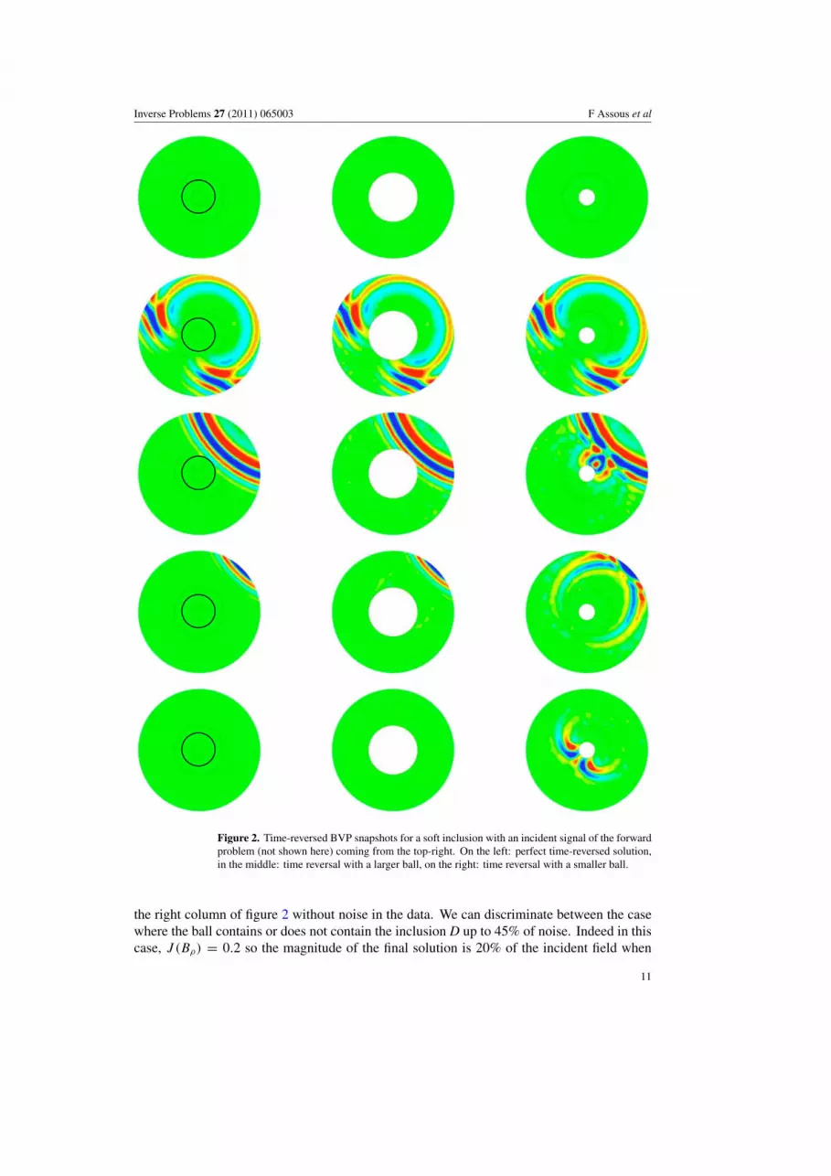
As a first test case, we consider an inclusion that is a soft disk and Bρ is a disk of thevariable radius. In figure 2, we have several rows and three columns. Each column correspondsto a numerical time-reversed experiment and each row corresponds to a snapshot of the solutionat a given time. The top line corresponds to the initial time for the time-reversed problem,equivalent to t = Tf for the forward problem. The last line is the solution at the final time ofthe reversed simulation which corresponds to the initial time t = 0 for the forward problem.In the left column, we display the perfect time reverse solution which is the reverse of theforward problem. For the inverse problem, the data is not known. It is shown for referenceonly.
In the middle column, we display the solution of the reversed problem (18) with a ball Bρ
which encloses the inclusion. As expected, the sequence of snapshots is the restriction to thedomain � \ Bρ of the left column. This exemplifies one application of the TRAC method: ifwe know that the ball Bρ encloses the inclusion we are able to reconstruct the signal in a regionthat is closer to the inclusion than the line of receivers �R . This allows for the reduction ofthe size of the computational domain. In this respect, the method is related to the redatumingmethod, see [7]. In the last column we show the solution of the reversed problem (18) with aball Bρ smaller than the soft disk. In contrast to the previous case, the sequence of snapshotsdiffers from the left column.
For the inverse problem of locating the scatterer, we only know that at the final time thesolution should be 0. In the middle column, this criterion is satisfied and we can thus inferthat the inclusion D is included in the ball Bρ . On the other hand, when the final solution inthe last column is not zero it shows that D is not included in the ball Bρ . This observationleads to an easy to compute criterion which is independent of the size of the domain:
J (Bρ) :=∥∥uT
R(Tf , ·)∥∥L∞(�\Bρ)
supt∈[0,Tf ] ‖uI (t, ·)‖|L∞(�)
(34)
which vanishes when the artificial ball encloses the inclusion. Due to numerical errors and thefact that the TRAC is not an exact ABC, the criterion is small but not 0, see figure 5.
Inverse problems are frequently ill-posed. Hence, a crucial question is the sensitivityof the method with respect to noise in the data. Therefore, we shall add Gaussian noise byreplacing the recorded data uT on �R by
uT := (1 + Coeff ∗ randn) ∗ uT , (35)
where randn satisfies a centered reduced normal law and Coeff is the level of noise. Thesolutions at the final time are depicted on figure 3. The level of noise is between 10% and50%. On the top line we display the results for a ball larger than the inclusion. Due to thenoise, the final solution is no longer zero but is a random signal of size related to the levelon noise. In the bottom line we display the result when the ball is smaller than the inclusion.Now, together with a random signal a structured non-zero solution appears which looks like
10
Inverse Problems 27 (2011) 065003 F Assous et al
Figure 2. Time-reversed BVP snapshots for a soft inclusion with an incident signal of the forwardproblem (not shown here) coming from the top-right. On the left: perfect time-reversed solution,in the middle: time reversal with a larger ball, on the right: time reversal with a smaller ball.
the right column of figure 2 without noise in the data. We can discriminate between the casewhere the ball contains or does not contain the inclusion D up to 45% of noise. Indeed in thiscase, J (Bρ) = 0.2 so the magnitude of the final solution is 20% of the incident field when
11

Inverse Problems 27 (2011) 065003 F Assous et al
Figure 3. Time-reversed solutions at the final time for noise on the recorded data from left to right:10%, 30%, 45% and 50%, for a ball larger than the inclusion on the top and a smaller ball on thebottom.
Table 1. Results of J (Bρ) for inclusions that do not intersect the artificial balls, see figure 4(a).
Radius Radius Radius Results for Results forinclusion large ball small ball large ball small ball
2λ 5.2λ λ <5% 100%λ 5.2λ λ <5% 100%λ 3.2λ λ <5% 100%0.5λ 5.2λ λ <5% 50%0.5λ 2.2λ λ <5% 50%
the ball Bρ encloses the inclusion whereas J (Bρ) = 0.6 when the ball does not enclose theinclusion. Thus, the method TRAC appears to be relatively insensitive to noise on the recordeddata.
In previous tests, for the sake of simplicity, the artificial balls and the inclusion wereconcentric. We now consider the case where either the artificial ball and the inclusion D donot intersect or the artificial ball crosses D without including or being included, see figure 4.Results are shown in tables 1 and 2. In table 1, the inclusion is between the artificial boundaries.Since in our tests the source emits from the North–East, we place the inclusion respectively inNorth–East, North–West, South–West and South–East for table 2. The radius of the inclusionis 1.35λ, the radius of the larger ball is about 3λ and the radius of the smaller one is alwaysλ. In all these cases, the criterion J (Bρ) discriminates between the possibilities since it takesvalues smaller than 0.05 when the artificial ball encloses the inclusion whereas it lies between0.3 and 1.0 in the other cases. Moderate values of the criterion (J (Bρ) = 0.3) correspond toa situation where the inclusion is in the shadow of the ball.
As a second test case we illustrate the TRAC method by taking penetrable inclusions withspeeds that correspond to medical applications. The value of the speed in the backgroundmedium is c = 1 and in the inclusion the values are taken from [24]: c = 1.7 (breast tumor),c = 1.14 (fibroadenoma) and c = 0.93 (surrounding tissue). We again stress that the method
12

Inverse Problems 27 (2011) 065003 F Assous et al
(a) (b)
Figure 4. (a) Inclusion between the artificial boundaries and (b) inclusion crossing the artificialboundaries.
Table 2. Results of J (Bρ) for an inclusion crossing the artificial balls, see figure 4(b).
Geographical Results for Results forposition large ball small ball
N–E <5% 65%N–W <5% 70%S–W <5% 30%S–E <5% 75%
does not rely on any a priori knowledge of the data. For these inclusions, the ball and theinclusion are concentric disks and we vary the size of the artificial balls. In figure 5, weplot the criterion J (Bρ) as a function of the distance between the inclusion and the artificialballs for various penetrable bodies. When the abscissa is negative, the ball does not enclosethe inclusion. J (Bρ) is even larger when the ball is smaller than the inclusion. The criterionincreases with the distance between the ball and the inclusion. On the other hand, when the ballencloses the inclusion (i.e., the abscissa is positive) the criterion is smaller than 0.1 and nearlyflat. Note, that as expected, the larger the contrast between the inclusion and the surroundingmedium the larger is J (Bρ). We have performed other experiments with inclusions of variousshapes. One such example is given later for the Helmholtz equation. In all cases, theresults are independent of the shape of the inclusion as long as its size is greater than onewavelength.
In conclusion, when we enclose the body with Bρ then J (Bρ) is small. When the balldoes not include the body D then the size of J (Bρ) indicates the distance between the scattererand the artificial ball.
13

Inverse Problems 27 (2011) 065003 F Assous et al
0 0.05 0.1−0.05−0.1
0.25
0.50
0.75
soft object c = 0
breast tumor c = 1.7
surrounding tissues c = 0.93
♦
♦
♦ ♦♦
♦♦ ♦ ♦ ♦ ♦
♦ fibroadenoma c = 1.14
Figure 5. Criterion J (Bρ) versus the algebraic distance between the inclusion and the artificialballs for various penetrable inclusions.
3.2. The Helmholtz equation
For the harmonic case, we again consider a scatterer D surrounded by a homogeneous andisotropic medium with a velocity of sound denoted by c0. The inclusion is illuminated by anincident field uI. Equation (8) becomes{−ω2 uT − c2�uT = 0 in R2
(uT (�x) − uI (�x)) satisfies a Sommerfeld condition at ∞.(36)
In order to create synthetic data, equation (36) is approximated by the FreeFem++ package[17] which constructs a finite element method in space. The incident wave is simulated by thesame procedure with a uniform velocity of sound equal to c0. We then introduce a boundary�R where the signal is recorded. The boundary �R encloses a domain denoted by �, seefigure 1. The next stage of the method is to introduce a ‘trial’ surface Bρ and solve the phaseconjugated problem (22) in � \ Bρ using an absorbing boundary condition. In contrast tothe time-dependent case, we cannot use the criterion defined in (34) since in the harmoniccase, there is no time and thus no final time. We define, later, two new criteria adapted to theharmonic case. We first look at the numerical simulations obtained with artificial balls anda soft square shaped inclusion that are concentric, see figure 6. In the top-left figure we plotthe modulus of the total field |uT | which coincides with the modulus of its conjugate field|uT |. On the right, we display the field obtained by the phase-conjugation method presentedin section 2.2, see equation (9). We see that there is a large difference between the total fieldand the field reconstructed by the phase conjugation method. The two bottom figures illustratethe TRAC method. In the left figure, the ball encloses the square and the computed field is the
14

Inverse Problems 27 (2011) 065003 F Assous et al
Figure 6. Phase conjugation for a soft square shaped inclusion of length 2 λ. From left to right,from top to bottom: perfect, phase conjugation, TRAC with a ball enclosing the inclusion, TRACwith a ball inside the inclusion.
restriction of the total field. In the right figure, the ball is inside the square and the computedfield is very different from the total field.
In practice, we do not know the total field and we have to introduce a way to measurewhether the artificial ball encloses the inclusion or not. For this purpose, we introduce twodifferent criteria. The first one is based on Dirichlet and Neumann data and the second oneis based on the TRAC method. The latter will prove to be more robust with respect to noisewithout requiring regularization techniques. For the first criterion, we assume that in additionto the total field uT we have also recorded the value of the normal derivative ∂uT /∂n on theboundary �R . When the ball encloses the inclusion, the normal derivative of the solution to thephase conjugation problem (22) coincides with the conjugation of the corresponding recordeddata. Thus, we introduce the following first criterion:
JDN(Bρ) :=∥∥ ∂uT
R
∂n− ∂uT
∂n
∥∥L∞(�R)∥∥ ∂uT
∂n
∥∥L∞(�R)
. (37)
The second criterion is derived from the TRAC method itself. Indeed, the basis of the methodis that the phase conjugated scattered field
uS := uT − uI
satisfies
TRAC(uS) = TRAC(uT − uI ) = 0 (38)
at any point outside the inclusion. In equation (22) this relation is used on the boundaryof the artificial ball Bρ . Since uT is computed numerically and uI is given data, that isreadily available at any point in � \ Bρ . Equation (38) can be computed at any point in �.
15

Inverse Problems 27 (2011) 065003 F Assous et al
Figure 7. Boundary �JABC inside the region for the new criterion JABC.
Thus, following the principle of the TRAC method, we introduce a new boundary �JABC (seefigure 7) to design a new criterion:
JABC(Bρ, �JABC) :=∥∥TRAC
(uT
R − uI)∥∥
L∞(�JABC )∥∥TRAC(uI )∥∥
L∞(�JABC )
. (39)
Note, that this criterion is not based on a direct comparison between numerical data andrecorded data in contrast to the first criterion. Hence, it does not require any additionalrecorded data. The criterion JABC, equation (39), could be used everywhere. However, sinceits accurate computation has some cost, we introduced a curve �TRAC on which we computeit.
Both criteria (37) and (39) should be 0 when the artificial ball Bρ encloses the inclusion.Since the TRAC is not derived from an exact ABC, the above criteria are small but not zero.Since, equation (38) is imposed on ∂Bρ in order to compute uT
R (see equation (22)), we haveto take �JABC different from ∂Bρ .
We tested both criteria for a soft circular inclusion of radius two wavelengths (2 λ) withvarious noise magnitudes on the recorded data defined as in (35). The radius of the artificialball can be as small as one wavelength and still avoid difficulties because of the absorbingboundary, with a small radius. The results are summarized in table 3. The results of theenclosing case correspond to a concentric artificial ball Bρ of radius 3 λ and the results of anon-enclosing ball correspond to a concentric ball of radius λ. The first criterion JDN worksonly up to 5% noise. However, the use of a filtering technique could improve the domainof validity of this criterion. The second criterion JABC enables one to discriminate betweenthe enclosing and non-enclosing cases up to 30% noise even though we have not filteredthe data. This robustness can be explained by the fact that the noise comes from boundarymeasurements while, the Helmholtz equation has regularizing properties so that the computedfield uT
R is much less noisy on the internal boundary �JABC than on the boundary �R .In the last experiment, we consider a soft inclusion with a non-smooth shape. We use
the TRAC method to detect the location of the inclusion by varying the respective locationsof the artificial ball. The results are summarized in table 4. First we take a large ball Bρ sothat we check that the inclusion D is not too close to the boundary �R . Then, we move Bρ tothe left. The high value of the criterion shows us that the inclusion D is not included inside.The third and fourth show other failed attempts to enclose the inclusion. The last columncorresponds to a successful location of the inclusion. This shows the possibility, by trial and
16

Inverse Problems 27 (2011) 065003 F Assous et al
Table 3. Values of the various criteria for several levels of noise.
JDN JABC
Noise magnitude Enclosing Non enclosing Enclosing Non enclosing
0% 5.04% 69.20% 6.34% 69.18%5% 46.38% 93.55% 12.79% 71.62%10% 103.40% 91.77% 13.55% 70.87%20% 213.65% 231.30% 35.99% 80.23%30% 301.46% 269.07% 51.03% 87.80%40% 532.97% 374.67% 57.99% 84.34%50% 644.47% 552.57% 63.28% 124.30%
Table 4. Criterion JABC for a soft inclusion and various ball locations.
Cases
JABC 8.52% 66.09% 60.28% 28.35% 11.89%
error, of recovering the approximate location of the inclusion. In future work we will try toreplace the trial and error procedure by an iterative technique.
4. Conclusion
We introduce the time-reversed absorbing conditions (TRAC) for time-reversal methods. Theyenable one to ‘recreate the past’ without knowing the source which has emitted the signalsthat are back-propagated. This is made possible by removing a small region surrounding thesource. We present two applications in inverse problems: the reduction of the size of thecomputational domain and the determination of the location of an unknown inclusion fromboundary measurements. We stress that in contrast to many methods in inverse problems, thismethod does not rely on any a priori knowledge of the physical properties of the inclusion.Hard, soft and penetrable inclusions are treated in a similar way. The feasibility of the methodwas shown with both time-dependent and harmonic examples. Moreover, the method hasproved to be fairly insensitive with respect to noise in the data.
References
[1] Antoine X, Barucq H and Bendali A 1999 Bayliss–Turkel like radiation conditions on surfaces of arbitraryshape J. Math. Anal. Appl. 229 184–211
[2] Assous F, Kray M, Nataf F and Turkel E 2010 Time reversed absorbing conditions C. R. Math. 348 1063–7[3] Bardos C and Fink M 2002 Mathematical foundations of the time reversal mirror Asymptotic Anal. 29 157–82[4] Barucq H, Djellouli R and Saint-Guirons A 2009 Performance assessment of a new class of local absorbing
boundary conditions for elliptical- and prolate spheroidal-shaped boundaries Appl. Numer. Anal. 59 1467–98
17

Inverse Problems 27 (2011) 065003 F Assous et al
[5] Bayliss A, Gunzburger M and Turkel E 1982 Boundary conditions for the numerical solution of elliptic equationsin exterior regions SIAM J. Appl. Math. 42 430–51
[6] Bayliss A and Turkel E 1980 Radiation boundary conditions for wave-like equations Commun. Pure Appl.Math. 33 707–25
[7] Berryhill J 1979 Wave-equation datuming Geophysics 44 132944[8] Blomgren P, Papanicolaou G and Zhao H 2002 Super-resolution in time-reversal acoustics J. Acoust. Soc.
Am. 111 230–48[9] Clouet J F and Fouque J P 1997 A time-reversal method for an acoustical pulse propagating in randomly layered
media Wave Motion 25 361–8[10] Colton D, Coyle J and Monk P 2000 Recent developments in inverse acoustic scattering theory SIAM
Rev. 42 369–414 (electronic)[11] Colton D and Kirsch A 1996 A simple method for solving inverse scattering problems in the resonance region
Inverse Problems 12 383–93[12] Colton D and Kress R 1998 Inverse Acoustic and Electromagnetic Scattering Theory (Applied Mathematical
Sciences vol 93) 2nd edn (Berlin: Springer)[13] Curlander J and McDonough R 1991 Synthetic Aperture Radar (New York: Wiley)[14] Engquist B and Majda A 1977 Absorbing boundary conditions for the numerical simulation of waves Math.
Comput. 31 629–51[15] Fink M 2009 Renversement du temps, ondes et innovation (College de France: Fayard)[16] Fink M, Wu F, Cassereau D and Mallart R 1991 Imaging through inhomogeneous media using time reversal
mirrors Ultrason. Imaging 13 199[17] Hecht F 2010 FreeFem++ numerical mathematics and scientific computation. Laboratoire J.L. Lions, Universite
Pierre et Marie Curie, http://www.freefem.org/ff++/, 3.7 edition[18] Kriegsmann G, Taflove A and Umashankar K 1987 A new formulation of electromagnetic scattering using on
surface radiation condition approach IEEE Trans. Antennas Propag. AP35 153–61[19] Larmat C, Montagner J-P, Fink M, Capdeville Y, Tourin A and Clevede E 2006 Time-reversal imaging of
seismic sources and application to the great sumatra earthquake Geophys. Res. Lett. 33 L19312[20] Lehman S K and Devaney A J 2003 Transmission mode time-reversal super-resolution imaging J. Acoust. Soc.
Am. 113 2742[21] Medvinsky M and Turkel E 2009 On surface radiation conditions for an ellipse JCAM 234 1647–55[22] Medvinsky M, Turkel E and Hetmaniuk U 2008 Local absorbing boundary conditions for elliptical shaped
boundaries J. Comput. Phys. 227 8254–67[23] Prada C, Manneville S, Spoliansky D and Fink M 1996 Decomposition of the time reversal operator: application
to detection and selective focusing on two scatterers J. Acoust. Soc. Am. 99 2067–76[24] Sinkus R, Tanter M, Xydeas T, Catheline S, Bercoff J and Fink M 2005 Viscoelastic shear properties of in vivo
breast lesions measured by mr elastography 23 159–65[25] Therrien C W 1992 Discrete Random Signals and Statistical Signal Processing (Englewood Cliffs, NJ: Prentice-
Hall)
18


