Title: Measuring developmental noise in bilateral traits

Title: Measuring developmental noise in bilateral traits.

Authors and Institutions:

Darryl J. Holman1, Laura L. Newell-Morris1, Carrie M. Kuehn, Christina M. Giovas1,

Robert E. Jones3, Ann Streissguth2

1 Department of Anthropology

2 Department of Psychiatry and Behavioral Science

University of Washington

Seattle, WA 98195 USA

3 Center for Demography and Ecology

University of Wisconsin-Madison

Madison, WI 53706 USA

Total Number of Pages: 33 Number of Figures: ? Number of Tables: ? Number of Footnotes: ? Number of References: ? Abbreviated title: Measuring developmental noise

Send Proof to: Darryl Holman Department of Anthropology University of Washington Box 353100 Seattle, WA 98195 USA Phone: (206) 543-7586 Email: [email protected]

Keywords: Fluctuating asymmetry, Directional asymmetry, Antisymmetry, measurement error,

developmental homeostasis.

2

Introduction

The body plan of most animals includes a major longitudinal axis of symmetry. Most structures

develop along this axis as nearly identical antimers, that is, they are expressed as mirror images of one

another. The genome of the developing embryo is believed to contribute equally to both sides of these

bilateral structures, so that there is an expectation that antimers will be symmetrical. Usually the

structures do not achieve perfect symmetry; instead, phenotype is expressed with small deviations from

perfect symmetry, that represent a departure from an ideal developmental plan encoded by genes (Van

Valen 1962).

For a half-century biologists have used departures from perfect symmetry as a means of

exploring the nature of development, developmental stability, and the effects of endogenous and

exogenous stresses on development. Many exogenous stressors are predicted to elevate asymmetry in

individuals, especially in areas or structures where developmental homeostasis is low and easily

disrupted (Livshits and Kobyliansky 1991). Endogenous disturbances like chromosomal abnormalities,

Mendelian-transmitted disease, and mulitfactorial hereditary defects have been shown to increase the

asymmetry of traits such as dermatoglyphic ridge counts (Kobylianski et al. 2000).

The tool most commonly used in investigations of asymmetry has been the distribution of left-

minus-right (LMR) values of a character. This distribution has been used to quantify two types of

bilateral asymmetry: directional asymmetry (DA) and fluctuating asymmetry (FA). Directional

asymmetry is the condition in which the trait on one side has a larger measure, on average, than its

counterpart. Directional asymmetry is usually quantified as the mean of the LMR distribution. A mean

of zero implies no DA and values that differ significantly from zero are evidence for DA.

Fluctuating asymmetry quantifies random deviations from perfect symmetry that occur when

antimeres are not perfect mirror images of each other. A number of indices have been developed for

quantifying fluctuating asymmetry. Nearly all of them are based on the variance (or standard deviation)

of the distribution of LMR differences (Palmer and Strobeck 1986). A variance near zero in this

distribution reflects perfect symmetry.

3

A third type of asymmetry, called antisymmetry (AS) arises when there is consistent DA within

individuals, but that the direction of the asymmetry is distributed randomly among individuals. In other

words, one of the antimeres tends to be consistently larger for each individual, but among individuals

there is no apparent bias for one side or the other. A well-known example of AS in nature is the

asymmetric claws on the male fiddler crab. Subtle examples of AS are not as widely recognized,

perhaps because the tools to distinguish AS from other types of asymmetry have not been available.

In this paper, we develop a new approach for investigating asymmetries. Rather that using the

LMR distribution as the basis for quantifying asymmetry, our approach is to estimate a distribution of

developmental noise along with the distribution of the trait itself. We base this approach, to the extent

possible, on the processes believed to bring about the expression of bilateral traits. As a result, the

parameters estimated for particular traits should provide insight into developmental processes and

disruptions by which asymmetries arise.

We begin by discussing some of problems and limitations inherent in the traditional methods for

studying asymmetries and developmental noise. Next, we describe the new method for directly

investigating developmental stability that is applicable to a wide variety traits, and solves many of the

problems encountered by the traditional analytic methods. Finally, we provide a number of examples of

the new method.

Standard Approaches to Measuring Asymmetry

Current approaches to the study developmental noise depend almost entirely on estimating

indices of FA and DA. A plethora of indices have been proposed, and nearly all are based on the

distribution of LMR differences between bilateral traits. Detailed descriptions of different methods, and

comparisons among them can be found elsewhere (Palmer and Stroebeck, 1986; Palmer, 1994; Møller

and Swaddle, 1997). For our purposes it is sufficient to point out that the most basic forms for

measures of DA and FA are Mean(L – R) and Var(L – R), respectively. Additionally, for a trait with

no DA, Mean(| L – R |) is another way to characterize the dispersion of the LMR distribution, and can

form the basis of a measure of FA.

4

A fundamental problem with current methods for assessing FA is that they are not based on a

specific etiologic model of developmental noise and measurement error. It is the non-etiologic nature of

the FA indices that leads, in part, to analytical difficulties and hinders interpretation. Some of the

problems of using and interpreting FA (and to a lesser extent, DA) are as follows:

Different index, different result: Different FA indices can produce different results on the

same data, making interpretation unclear. No single index is considered clearly superior under all

circumstances. Palmer and Stroebeck (1986), after examining many different indices, and after

analyzing different simulated data sets, found no universally superior index. They recommend computing

and reporting several indices. Clearly, a single index that provides an unambiguous result is preferred to

multiple, and possibly conflicting, indices.

Non-normal traits and discrete traits: A universal approach has not been developed for

working with traits that are not normally distributed. As discussed later in this paper we should exploit

the very reasonable assumption that developmental noise is normally distributed. Yet, the LMR

distribution is not, in general, normally distributed. For example, if the bilateral trait is distributed as a

negative exponential, then the resulting distribution of LMR differences is a Laplace (or double

exponential) distribution (Johnson et al. 1995). Ad hoc versions of FA indices have arisen in response.

A related problem arises in working with meristic (discrete) traits that have low trait counts.

Indices of FA are based on continuous traits, so that ad hoc adjustments are typically used with meristic

traits (Palmer and Stroebeck 1986; M∅ller and Swaddle 1997).

Incompletely observed traits: A difficulty arises when the bilateral trait under investigation is

incompletely observed. For example, traits that are measured as the timing to some bilateral event

(suture closure, tooth emergence, etc.) can entail right-censoring of one or both of the measurement

pairs. Additionally, these traits are usually measured over an interval, rather than as an exact time to the

event. The interval encloses the unobserved time. This type of observation referred to as interval-

censored in the statistical literature. Methods to assess asymmetry in interval-censored traits have never

been developed. For this reason some type of bilateral traits—particularly those that are timings to

some developmental stage—have rarely been explored.

Exploring asymmetry. The traditional methods are not conducive to exploring the causes and

nature of asymmetries. For example, there is no reason to believe that FA cannot be measured as a

5

signal on top of AS. Likewise, directional effects can be considered a continuous spectrum that begins

with DA (where a size bias arises 100% to one side) to AS (where the size bias occurs 50% to one

side). Finally, an understanding of how FA, DA, and AS arise and are affected by endogenous and

exogenous stresses requires that we simultaneously model all three asymmetries. Furthermore, we

should be able to incorporate the effects of covariates on the properties of asymmetries. Current

methods lack this degree of flexibility.

Measurement Error: It was recognized early on that measurement error can severely affect

estimates of FA (REF). This is because the variance in the LMR distribution is the sum of the variance

arising out of true differences and the variance resulting from errors of measurement. Some methods

have been developed that disentangle FA from measurement error given repeated measures of each

trait. Palmer and Stroebeck (1986) introduced a two-way mixed analysis of variance (ANOVA)

framework (see also, Møller and Swaddle 1997; Boklage 1992). The ANOVA framework provides

for systematic tests of hypothesis about fluctuating and directional asymmetry, and can be used to

examine effects of other covariates (e.g. sex, treatment). The technique yields a single error-adjusted

variance computed using repeated measurements (Palmer 1994). More recently, Van Dongen and

colleagues (1999) have proposed a mixed regression model that yields the same results as the

ANOVA, but provides a more direct interpretation of estimated parameters, allows for more flexibility

for hypothesis testing, and can be used to estimate individual error-corrected estimates of FA.

Methods

Measuring developmental noise

We have developed a new approach to quantifying developmental noise in bilateral traits. The

approach is motivated by simple biological principles, and we believe it can be broadly applied to the

study of asymmetries. Briefly, the difference between our approach and previous approaches is that our

6

method simultaneously estimates two parametric distributions from pairs of bilateral traits: (1) a

distribution of developmental noise and (2) a single distribution for the underlying trait. The first

distribution, developmental noise, is expected to be normally distributed (although even this assumption

is easy to relax). In the absence of directional asymmetry, the distribution of developmental noise will

have a mean of zero and a variance that characterizes the developmental noise. The second distribution

represents the distribution of the underlying phenotype, unmodified by developmental noise. This

distribution need not be (and arguably should rarely be) a normal distribution. Some of the difficulty

encountered using the traditional approaches is that distribution of the trait and the distribution of

developmental noise are confounded.

We are able to estimate both distributions using maximum likelihood to estimate parameters.

The method should have broad applicability for a wide variety of traits and missing data situations.

Simple extensions of the method allow for quantification of the effects of covariates. The covariates can

be modeled as affecting the bilateral trait in several ways. They can affect the variance in developmental

noise, akin to increase or decrease in fluctuating asymmetry. Covariates effects can also be modeled as

affecting the mean of the underlying trait. For example, disturbances might retard the rate of

development, resulting in longer mean times to developmental events. Third, the covariates might affect

the variance of the underlying trait. For example, the expression of a trait in individuals exposed to an

environmental perturbation might be more variable, but with the same mean as individuals not exposed.

Finally, covariates can affect directional asymmetry in a number of ways.

In the following section we provide details of the new approach, beginning with the simplest

case of a continuous trait. We then generalize the basic model to incorporate discrete traits, directional

asymmetry, time-varying covariates, measurement error, and incomplete observations. The result is a

flexible approach that overcomes many of the disadvantages of the standard methods used to quantify

FA.

We begin with a single bilaterally symmetric trait, denoted by random variable T. Trait T is

distributed according to probability density function (PDF) fT(t; µT, σT), where µT and σT are the

location and scale parameters respectively. For now, we need not specify any particular distribution of

the trait T, although a normal or a lognormal distribution tends to be used for many continuous traits

(Wright 1968). For all traits, it is difficult or impossible to measure specific values of ti (the value of t

7

for the i-th individual) because of the presence an unknown amount of developmental noise and

measurement error superimposed on ti. Hence, T is a latent random variable because it cannot be

measured directly.

Instead of measuring ti for individual i, we can measure li and ri, the left and right measurements

of the bilateral trait. Aside from a common but unmeasureable value of ti, measurements li and ri also

include developmental noise and possibly measurement error. Call A a random variable that describes

all sources of departures from the true values of T. In particular, A includes developmental noise (which

will be represented by random variable D) and measurement error (which will be represented by

random variable E).

Random variables for the left and right measurements (L and R respectively) share a common

value T and the bilateral measurements provide information on two independent realizations of A.

(1) l l l

r r r

L T A T D ER T A T D E

= + = + += + = + +

.

Note that we do not subscript T for each side. This results from the assumption that the trait is a single

phenotype that is expressed identically on both sides. When A is subdivided into its two components, E

can frequently be assumed normally distributed with a mean of zero. The variance of A is σA2 = σD

2 +

σE2, where σD

2 is the variance attributable to developmental noise, and σE2 is the variance in

measurement error.

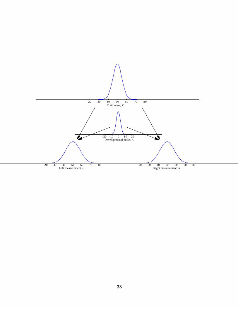
A graphical representation is given in Figure 1. The top of the figure shows the distribution of

the trait, T. Added to T are two values drawn from the distribution of developmental noise (and

perhaps measurement error) shown as the distributions in the center. The result are the two distributions

of measured values (L and R) shown on the bottom.

We begin with the simplest model in which E is minimal, which corresponds to the case where

traits can be measured in a way that ensures a very small measurement error. This assumption is used

when repeated measures are not available for each side to separate A into its two components. The

PDF of A is denoted g(a|0, σA); usually we can assume A is normally distributed with a mean of zero

and a variance of σA2.

8

Suppose for a moment that ti, ali, and ari could be measured directly in a sample of N

individuals. For each individual, we would have a single realization from T, and two independent

realizations from A, one left and right, with a mean of zero and a common variance. It would the be

simple to estimate parameters for the three distributions fT(t|µT, σT), g(aL|0, σA), and g(aR|0, σA). If the

distributions were Normal, estimates of µT, σT could be obtained as a mean and standard deviation

from the array of N measurements t = (t1, t2, ... tN). Likewise, σa could be found as the standard

deviation among N measurements aL = (aL1, aL2, ... aLN) and aR= (aR1, aR2, ... aRN). An alternative

method of finding µT, σT and σA is maximum likelihood. The likelihood for the i-th individual would be

constructed as the product of values of the three distributions as

(2) ( , , | , , ) ( | , ) ( |0, ) ( |0, )i T T A i Li Ri T i T T A Li A A Ri AL t a a f t g a g aµ σ σ = µ σ σ σ .

The likelihood over all N individuals would be the product of the individual likelihoods, or

(3) 1

( , , | , , ) ( | , ) ( |0, ) ( |0, )N

T T A T i T T A Li A A Ri Ai

L f t g a g a=

µ σ σ = µ σ σ σ∏L Rt a a .

The values of µT, σT and σA that maximize L for a given set of observations are the maximum likelihood

estimates for these parameters.

One advantage of using the likelihood over the least-squares estimation is that any parametric

distribution can be specified for fT( ). For that matter, any parametric distribution can be used for gA( ),

as well. Additional advantages come from being able to build complex models to incorporate, for

example, measurement error, directional asymmetry, and the effects of covariates on the distributions, as

done in later sections.

So far, we have made the assumption that ti, aLi and aRi could be measured directly. In

practice we only have measurements li and ri from which to make inferences about parameters of fT( )

and gA( ). To construct a likelihood that only makes use of li and ri, suppose we could measure ti, li

and ri, but not aLi, and aRi. Then, given that li = ti + aLi and ri = ti + aRi, likelihood (3) would be

changed to

9

(4) 1

( , , | , , ) ( | , ) ( |0, ) ( |0, )N

T T A T i T T A i i A A i i Ai

L f t g l t g r t=

µ σ σ = µ σ − σ − σ∏t l r .

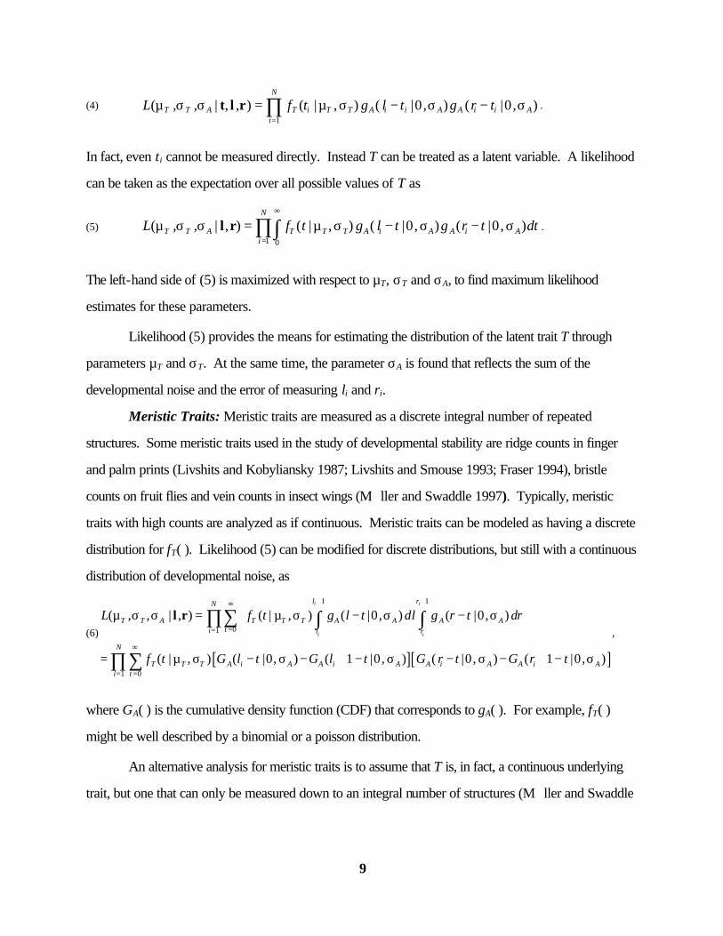
In fact, even ti cannot be measured directly. Instead T can be treated as a latent variable. A likelihood

can be taken as the expectation over all possible values of T as

(5) 1 0

( , , | , ) ( | , ) ( |0, ) ( |0, )N

T T A T T T A i A A i Ai

L f t g l t g r t dt∞

=

µ σ σ = µ σ − σ − σ∏∫l r .

The left-hand side of (5) is maximized with respect to µT, σT and σA, to find maximum likelihood

estimates for these parameters.

Likelihood (5) provides the means for estimating the distribution of the latent trait T through

parameters µT and σT. At the same time, the parameter σA is found that reflects the sum of the

developmental noise and the error of measuring li and ri.

Meristic Traits: Meristic traits are measured as a discrete integral number of repeated

structures. Some meristic traits used in the study of developmental stability are ridge counts in finger

and palm prints (Livshits and Kobyliansky 1987; Livshits and Smouse 1993; Fraser 1994), bristle

counts on fruit flies and vein counts in insect wings (M∅ller and Swaddle 1997). Typically, meristic

traits with high counts are analyzed as if continuous. Meristic traits can be modeled as having a discrete

distribution for fT( ). Likelihood (5) can be modified for discrete distributions, but still with a continuous

distribution of developmental noise, as

(6)

[ ][ ]

1 1

01

01

( , , | , ) ( | , ) ( |0, ) ( |0, )

( | , ) ( |0, ) ( 1 |0, ) ( |0, ) ( 1 |0, )

i i

i i

l rN

T T A T T T A A A Ati l r

N

T T T A i A A i A A i A A i Ati

L f t g l t dl g r t dr

f t G l t G l t G r t G r t

+ +∞

==

∞

==

µ σ σ = µ σ − σ − σ

= µ σ − σ − + − σ − σ − + − σ

∑∏ ∫ ∫

∑∏

l r,

where GA( ) is the cumulative density function (CDF) that corresponds to gA( ). For example, fT( )

might be well described by a binomial or a poisson distribution.

An alternative analysis for meristic traits is to assume that T is, in fact, a continuous underlying

trait, but one that can only be measured down to an integral number of structures (M∅ller and Swaddle

10

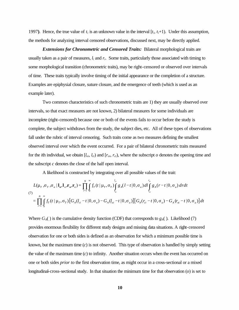
1997). Hence, the true value of ti is an unknown value in the interval [ti, ti+1). Under this assumption,

the methods for analyzing interval censored observations, discussed next, may be directly applied.

Extensions for Chronometric and Censored Traits: Bilateral morphological traits are

usually taken as a pair of measures, li and ri. Some traits, particularly those associated with timing to

some morphological transition (chronometric traits), may be right-censored or observed over intervals

of time. These traits typically involve timing of the initial appearance or the completion of a structure.

Examples are epiphysial closure, suture closure, and the emergence of teeth (which is used as an

example later).

Two common characteristics of such chronometric traits are 1) they are usually observed over

intervals, so that exact measures are not known, 2) bilateral measures for some individuals are

incomplete (right-censored) because one or both of the events fails to occur before the study is

complete, the subject withdraws from the study, the subject dies, etc. All of these types of observations

fall under the rubric of interval censoring. Such traits come as two measures defining the smallest

observed interval over which the event occurred. For a pair of bilateral chronometric traits measured

for the ith individual, we obtain [loi, lci) and [roi, rci), where the subscript o denotes the opening time and

the subscript c denotes the close of the half open interval.

A likelihood is constructed by integrating over all possible values of the trait:

(7)

[ ][ ]

1 0

1 0

( , , | , , , ) ( | , ) ( |0 , ) ( |0, )

( | , ) ( |0, ) ( |0 , ) ( |0, ) ( |0, )

ci ci

oi o i

l rN

T T a T T T A a A ai l r

N

T T T A ci a A oi a A ci a A oi ai

L f t g l t dl g r t drdt

f t G l t G l t G r t G r t dt

∞

=

∞

=

µ σ σ = µ σ − σ − σ

= µ σ − σ − − σ − σ − − σ

∏∫ ∫ ∫

∏∫

o c o cl l r r

Where GA( ) is the cumulative density function (CDF) that corresponds to gA( ). Likelihood (7)

provides enormous flexibility for different study designs and missing data situations. A right-censored

observation for one or both sides is defined as an observation for which a minimum possible time is

known, but the maximum time (c) is not observed. This type of observation is handled by simply setting

the value of the maximum time (c) to infinity. Another situation occurs when the event has occurred on

one or both sides prior to the first observation time, as might occur in a cross-sectional or a mixed

longitudinal-cross-sectional study. In that situation the minimum time for that observation (o) is set to

11

zero, and the maximum time (c) is set to the time of the first observation (Wood et al. 1992; Holman

and Jones 1998).

Paleontological samples present some analytical difficulties because individual specimens may

have fragmented or broken measures for one or both sides, or may simply be missing one of the two

measurements. Depending on the process by which missing observations arise, excluding incomplete

specimens can result in biased parameter estimates. Under some mild statistical assumptions,1 we can

use the same technique as we did for interval censored observations. A missing side is handled as

having a minimum length of zero and a maximum length of infinity. The missing side adds no information

to the distribution gA( ) on the missing side, but the side that is not absent contributes to a better

determination of fT( ) and gA( ). When one or both sides of a structure are incompletely preserved (i.e.

a portion has broken off and has been lost), the missing measurement may be treated as a right-

censored observation, taking the minimum length as the measured size and the maximum length as

infinity (or the maximum length possible in a confined grave).

Measurement Error: An important issue in the recent FA literature is the development of

methods to disentangle measurement error from developmental noise, as the measurement error for

some traits may swamp the developmental noise (Greene 1984; Palmer and Strobeck 1986; 1997;

Fields et al. 1995). The effects of measurement error and developmental instability can be disentangled

when repeated measures are available for each trait. With repeated measures we can refine the

methods so that the distribution gA( ) is now separated into a distribution of measurement error, gE( ),

and the distribution of developmental noise, gD( ).

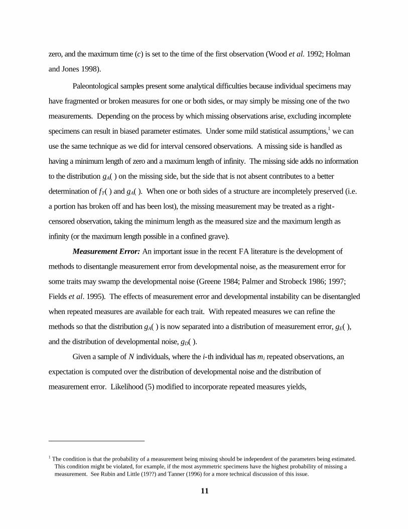
Given a sample of N individuals, where the i-th individual has mi repeated observations, an

expectation is computed over the distribution of developmental noise and the distribution of

measurement error. Likelihood (5) modified to incorporate repeated measures yields,

1 The condition is that the probability of a measurement being missing should be independent of the parameters being estimated. This condition might be violated, for example, if the most asymmetric specimens have the highest probability of missing a measurement. See Rubin and Little (19??) and Tanner (1996) for a more technical discussion of this issue.

12

(8)1 10

( , , , | , ) ( | , ) ( |0, ) ( |0 , ) ( |0, )imN

T T D E T T T E E D ij D D ij Di jx

L f t g e g l t e g r t e dedt∞ ∞

= =

µ σ σ σ = µ σ σ − − σ − − σ∏ ∏∫ ∫l r .

The other likelihoods are similarly modified to incorporate measurement error.

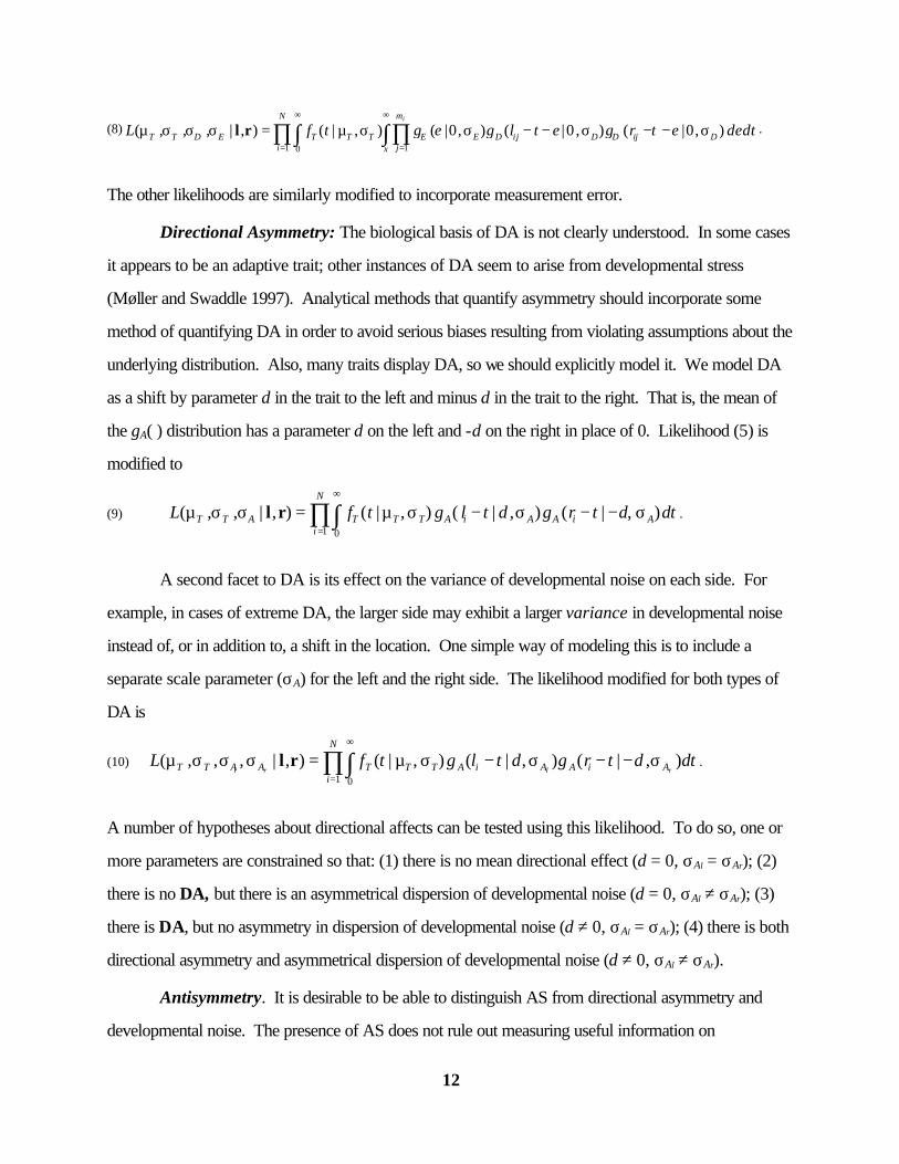
Directional Asymmetry: The biological basis of DA is not clearly understood. In some cases

it appears to be an adaptive trait; other instances of DA seem to arise from developmental stress

(Møller and Swaddle 1997). Analytical methods that quantify asymmetry should incorporate some

method of quantifying DA in order to avoid serious biases resulting from violating assumptions about the

underlying distribution. Also, many traits display DA, so we should explicitly model it. We model DA

as a shift by parameter d in the trait to the left and minus d in the trait to the right. That is, the mean of

the gA( ) distribution has a parameter d on the left and -d on the right in place of 0. Likelihood (5) is

modified to

(9) 1 0

( , , | , ) ( | , ) ( | , ) ( | , )N

T T A T T T A i A A i Ai

L f t g l t d g r t d dt∞

=

µ σ σ = µ σ − σ − − σ∏∫l r .

A second facet to DA is its effect on the variance of developmental noise on each side. For

example, in cases of extreme DA, the larger side may exhibit a larger variance in developmental noise

instead of, or in addition to, a shift in the location. One simple way of modeling this is to include a

separate scale parameter (σA) for the left and the right side. The likelihood modified for both types of

DA is

(10) 1 0

( , , , | , ) ( | , ) ( | , ) ( | , )l r l r

N

T T A A T T T A i A A i Ai

L f t g l t d g r t d dt∞

=

µ σ σ σ = µ σ − σ − − σ∏∫l r .

A number of hypotheses about directional affects can be tested using this likelihood. To do so, one or

more parameters are constrained so that: (1) there is no mean directional effect (d = 0, σAl = σAr); (2)

there is no DA, but there is an asymmetrical dispersion of developmental noise (d = 0, σAl ≠ σAr); (3)

there is DA, but no asymmetry in dispersion of developmental noise (d ≠ 0, σAl = σAr); (4) there is both

directional asymmetry and asymmetrical dispersion of developmental noise (d ≠ 0, σAl ≠ σAr).

Antisymmetry. It is desirable to be able to distinguish AS from directional asymmetry and

developmental noise. The presence of AS does not rule out measuring useful information on

13

developmental noise. Additionally, questions like the effect of stressors on antisymmetric traits might be

asked. Currently, these question are almost entirely unexplored. It is reasonable to suppose that

developmental noise will leave a signature superimposed on AS. Until recently, there have been few

methods for the analysis of traits exhibiting AS. Van Dongen, Lens and Molenberghs (1999)

introduced a method using finite mixture models to estimate FA, DA, and AS. We adopt a similar

mixture model approach to quantify AS, but within the framework of estimating developmental noise.

Under this approach, AS is assumed to represent a form of DA that is distributed between both sides.

For an individual observation, the largest side will usually, but not necessarily always, reflect the

direction in which development is biased. (It is conceivable that developmental noise added to the

smaller side or removed from the larger side will result in a side reversal of the side with the largest trait.)

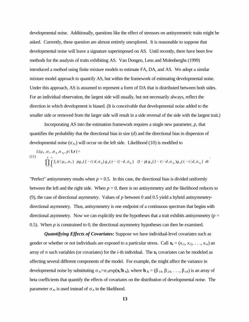
Incorporating AS into the estimation framework requires a single new parameter, p, that

quantifies the probability that the directional bias in size (d) and the directional bias in dispersion of

developmental noise (σA1) will occur on the left side. Likelihood (10) is modified to

(11)1 2

1 2 2 11 0

( , , , , | , )

( | , ) ( | , ) ( | , ) (1 ) ( | , ) ( | , )

T T A A

N

T T T A i A A i A A i A A i Ai

L p

f t pg l t d g r t d p g l t d g r t d dt∞

=

µ σ σ σ =

µ σ − σ − − σ + − − − σ − σ ∏∫

l r.

"Perfect" antisymmetry results when p = 0.5. In this case, the directional bias is divided uniformly

between the left and the right side. When p = 0, there is no antisymmetry and the likelihood reduces to

(9), the case of directional asymmetry. Values of p between 0 and 0.5 yield a hybrid antisymmetry-

directional asymmetry. Thus, antisymmetry is one endpoint of a continuous spectrum that begins with

directional asymmetry. Now we can explicitly test the hypotheses that a trait exhibits antisymmetry (p =

0.5). When p is constrained to 0, the directional asymmetry hypotheses can then be examined.

Quantifying Effects of Covariates: Suppose we have individual-level covariates such as

gender or whether or not individuals are exposed to a particular stress. Call xi = (x i1, x i2, . . ., x in) an

array of n such variables (or covariates) for the i-th individual. The xi covariates can be modeled as

affecting several different components of the model. For example, the might affect the variance in

developmental noise by substituting σAi=σAexp(xi'β A), where β A = (β1A, β2A, . . ., βnA) is an array of

beta coefficients that quantify the effects of covariates on the distribution of developmental noise. The

parameter σAi is used instead of σA in the likelihood.

14

The xi covariates might also affect other aspects of growth. For example, the size of the trait

itself might be affected some particular stress. This can be examined by replacing µT for an individual

measure µTi = µTexp(xi'β T), where β T = (β1T, β2T, . . ., βnT) is an array of beta coefficients that

quantify the effects of covariates on the mean of trait T. (Alternatively, the linear parameterization µTi =

µT + xi'β T can be used). Another possible effect of covariates might be to change the magnitude of

directional asymmetry, which is accomplished by substituting di = dexp(xi'β d) in place of d, where β d

= {β1d, β2a, . . ., βnd} is an array of beta coefficients.

Subjects

Asymmetry and developmental noise are estimated for several types of traits in two different

samples. The first is a sample of Javanese children for whom we examine asymmetry in developmental

noise in the time to emergence of deciduous teeth. The second is a sample of individuals with known

prenatal exposure to alcohol, as well as a group of unexposed controls. We examine the effect of

alcohol exposure on two dermatoglyphic traits: a-b ridge counts, and atd angle.

Deciduous tooth emergence in Javanese children. Data on bilateral emergence of

deciduous teeth come from the Ngaglik project, a three-year prospective investigation of maternal and

child health and nutrition, breastfeeding, and birth spacing dynamics carried out in the late 1970’s in

Central Java, Indonesia (Ngaglik Study Team 1978; Hull 1983). A description and previous analyses

of the dental data can be found elsewhere (Holman and Jones 1991, 1998; Hull 1983). Briefly, 468

children in two rural villages were examined for clinical emergence of deciduous teeth prospectively over

the two and one-half year course of the study. Children recruited into the study were from zero to six

months of age, but none had emerged a tooth at the first observation. Exact dates of birth and dates of

dental examinations are known. Interviews were scheduled every 35 days (one Javanese month);

however, about 5% were of emergence events were observed over a larger interval because one or

more visits were missed. Hence, times to emergence are always observed as the minimum time (to) and

the maximum possible time (tc) of emergence. Together, [to, tc) defined an interval within which

emergence occurs; for right censored observations, tc is set to infinity.

15

The timing of tooth emergence is modeled as being lognormally distributed beginning at one

month in utero. The use of a lognormal distribution for tooth emergence

Emergence age is shifted by a constant of eight months, back to one month after conception,

corresponding to the time when the dental lamina are initially formed (Ten Cate, 1998). Using

conception, or shortly thereafter, as the starting point for tooth emergence was suggested by Kihlberg

and Koski (1954) and Hayes and Mantel (1958), and has been used or discussed in a number of

previous studies (Holman and Jones, 1998; Magnússon, 1982; Smith et al., 1994). The distribution of

developmental noise is modeled as a normal distribution. A single trait, emergence of the lower central

deciduous incisor, is analyzed here.

a-b ridge count in children exposed to prenatal alcohol. Right and left hand prints were

obtained from individuals affected with fetal alcohol syndrome (FAS) or fetal alcohol effects (FAE) and

a control sample of individuals who reported that their mothers do not drink alcohol. The affected

sample was 193 subjects diagnosed with fetal alcohol syndrome (FAS) (29F, 39M) or fetal alcohol

effects (FAE) (52F, 73M). All affected individuals had been referred to the Fetal Alcohol Syndrome

Diagnostic Clinic at the University of Washington for diagnostic evaluation during 1994-95 for further

follow-up. The patients were typically referred for cognitive and behavioral problems, and had a

confirmed or suspected history of prenatal alcohol exposure. (Striessguth et al. 1996). At the time of

recruitment, ages of subjects ranged from 6-51 years of age, 74% were 6-11 years, 62%, 12-20 years

and 36%, 21-51 years.

The control sample of 190 subjects (80F, 110M) was recruited from students (19-35 years

old) at the University of Washington during the periods 1995-96 and 2001). All were screened for

eligibility by interview. Participants had no prior diagnosis as FAS/E, had no familial history of heritable

diseases or congenital defects, and reported that their mother did not consume alcohol.

Handprints were taken using the standard carbon-paper-tape technique (Reed and Meier

1990). The prints were scanned into digital images at 400 dots per inch resolution. Prints were

assesed for left and right a-b ridge count. Intraobserver error in ridge count error was XXX ridges and

for ATD angle was XXX degrees. After the prints were read the case number was used to identify the

individual characteristics like sex and diagnosis (FAS/E or Control).

16

Numerical methods and model selection

Maximum likelihood estimates of parameters were found by numerically evaluating likelihoods

using the mle programming language (Holman 2000). Estimates of the standard errors for all

parameters are found by the method of Nelson (1982), which involves inverting a numerical

approximation of Fisher's information matrix. Akaike Information Criterion (AIC) is used to select the

between competing forms of each models (Akaike 1973, 1992; Burnham and Anderson 1998). The

model that minimizes AIC is taken to be the most parsimonious model. (Alternatively, likelihood ratio

tests can be used, and we provide loglikelihoods for that purpose.)

Results

Developmental noise in tooth emergence. Parameter estimates for these interval- and

right-censored observations were found as those that maximize likelihood (7), modified to include the

directional asymmetry parameter (d) as in likelihood (9).

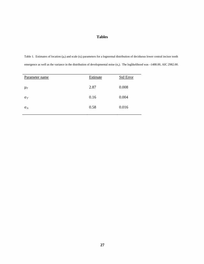
Parameter estimates for the simplest model that includes two parameters of the underlying trait

(µT, σT) and developmental noise (σA) are given in Table 1. Developmental noise was clearly identified

along with the underlying trait of tooth emergence time.

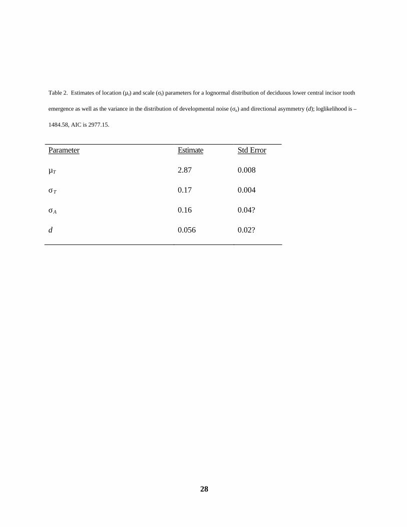
The bottom panel is an analysis that includes DA. Significant DA was found to the left. Clearly,

some of the variance in developmental noise found in the first analysis was an artifact of DA. Even after

when DA is estimated, developmental noise is still detectable. The difference between the two analyses

in Akaike Information Criteria indicate that the second analysis provides a better fit to the observations

even with one extra parameter.

a-b ridge count. Alcohol is a known teratogen and its effects on morphology and especially,

neurobehavior are well documented (Streissguth et al. 1994). Alcohol presents a potentially robust

stressor to the developing embryo/fetus; as a result, developmental instability is predicted to be

increased in the phenotype of an individual exposed prenatally. Kieser (1992) documented greater

17

odontometric asymmetry compared to controls in 112 non-FAS children of alcoholic mothers.

Significantly higher FA was found for the intercore ridge count in macaque monkeys experimentally

exposed to alcohol in utero (Newell-Morris, Mauer and Clarren 1997), the a-b ridge count in patients

diagnosed with FAS (Wilber, Newell-Morris and Streissguth 1993), and females diagnosed with

FAS/E (Kuehn et al. 2001).

For this analysis we treat the a-b ridge count as a continuous, normally distributed trait, and the

distribution of developmental noise as normally distributed. Parameters were estimated using likelihood

(5), modified for some analyses to include the directional asymmetry parameter (d) and for some the

effect of alcohol exposure on the distribution of developmental noise (βa). The results of a series of

analyses are given in Table 3.

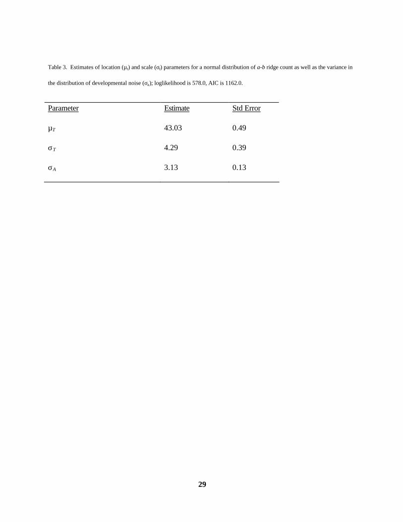
The first analysis estimates a mean ridge count of 43.0 and a standard deviation of 4.29. These

figures are close to the means and standard deviations estimated for the right (µ: 42.0, σ: 5.29) and left

ridge counts (µ: 44.1, σ: 5.17) separately. The standard deviation in developmental noise for the

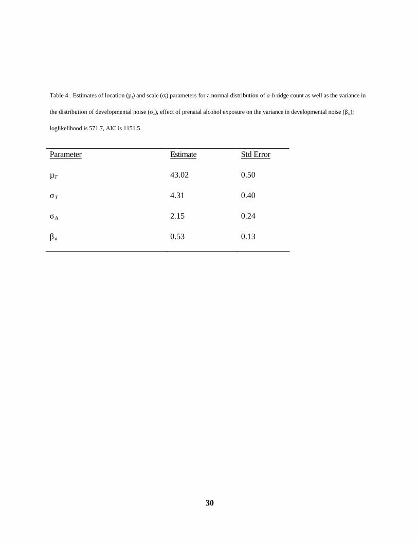
combined sample (affected and controls) was 3.13. In the second analysis, the effect of alcohol

exposure on the distribution of developmental noise (βa) is estimated. The value of 0.53 (SE 0.13) is

significantly different from zero, and indicates an increase in the standard deviation of the distribution of

developmental noise of about 70 percent. (A likelihood ratio test indicates that this second model fits

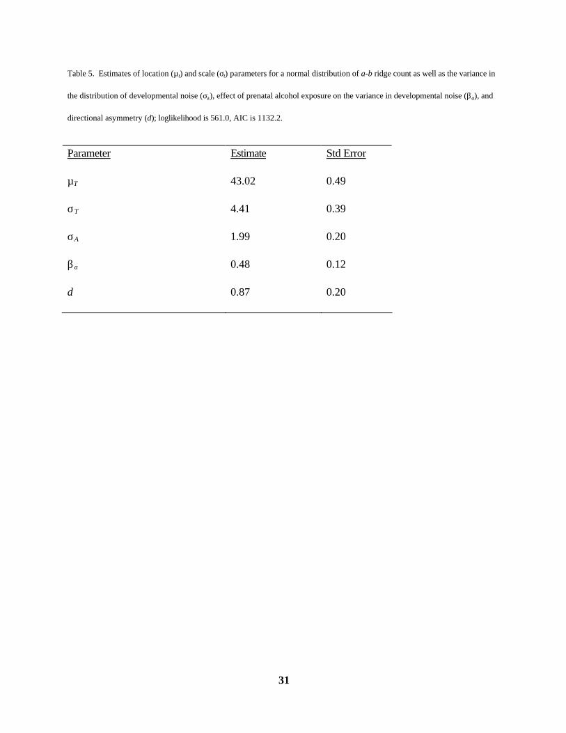
significantly better). For the third analysis, we add a parameter for directional asymmetry (d), which is

highly significant, and the AIC difference or likelihood ratio test indicates that this third model fits the

data much better. The directional asymmetry is slightly less than one excess ridge to the left. In this

third analysis, the βa parameter is still significant at p < 0.05, and indicates an increase in the standard

deviation of the distribution of developmental noise of about 62 percent after controlling for DA.

This analysis shows that modeling of DA is important when measuring the effects of stressors on

developmental noise. Although the biological mechanisms for subtle directional asymmetry (as exhibited

in the a-b ridge count trait) is poorly understood, there is evidence that stressors may act to amplify the

degree of DA (Graham, Freeman and Emlen 1994). A natural extension to the current analysis would

be to explicitly model an effect of prenatal exposure on the DA parameter (as outlined in the Statistical

Methods Section).

18

References cited

Akaike H (1973, 1992) Information theory and an extension of the maximum likelihood principle. In

Petrov BN and Csaki F (eds.), Second International Symposium on Information Theory.

pp. 268-81. Budapest: Hungarian Academy of Sciences. Reprinted in Kotz S and Johnson N

(eds.). Breakthroughs in Statistics. New York:Springer Verlag, pp. 610-24.

Arrieta MI, Criado B, Martinez B, Lobato MN, Gil A and Lostao CM. Fluctuating dermatoglyphic

asymmetry: genetic and prenatal influences. Ann Hum Biol 20: 557-63.

Babler WJ (1978) Prenatal selection and dermatoglyphic pattern. Am J Phys Anthropol 48: 21-8.

Babler WJ (1979) Quantitative differences in morphogenesis of human epidermal ridges. In: Wertelecki

W, Plato CC and Paul NW (eds). Dermatoglyphics-FiftyYears Later. New York, Wiley-

Liss, pp.199-208.

Babler WJ (1991) Embryonic development of epidermal ridges and their configurations. In: Plato CC,

Garruto RM and Schaumann BA (eds.). Dermatoglyphics: Science in Transition. New

York, Wiley-Liss, pp. 95-112.

Boklage CE (1992) Method and meaning in the analysis of developmental asymmetries. J Hum Ecol

Special Issue 2: 147-56.

19

Bookstein FL, Sampson PD, Streissguth AP and Connor PD (2001) Geometric morphometrics of

corpus callosum and subcortical structures in the fetal-alcohol-affected brain. Teratology 64:4-

32.

Bratley P, Fox BL and Schrage LE (1983) A Guide to Simulation New York: Springer-Verlag.

Brown NA, McCarthy A, Wolpert L (1991) Development of handed body asymmetry in mammals. In.

Bock GR and Marsh J (eds.) Biological Asymmetry and Handedness. Chichester:Wiley. pp.

198-201. (Documents the sensitive period of development and handedness).

Burnham KP and Anderson DR (1998) Model Selection and Inference: A Practical Information-

Theoretic Approach. New York: Springer Verlag.

Connor PD, Sampson PD, Bookstein FL, Barr HM and Streissguth AP (2000) Direct and indirect

effects of prenatal alcohol damage on executive function. Develop Neuropsychol 18: 331-54.

Cummins H. (1936) Dermatoglyphic stigmata in Mongolian idiocy. Anat Rec 64 (Suppl. 3):11.

Cummins H and Midlo C (1943) Finger Prints, Palms and Soles. South Berlin, Mass: Research

Publishing Co.

Dell DA and Munger BL (1986) The early embyogenesis of papillary (sweat duct) ridges in primate

glabrous skin: the dermatoglyphic map of cutaneous mechanoreceptors and dermatoglyphics. J

Comp Neurol 244: 511-32.

Fields SJ, Spiers M, Hershkovitz I, Livshits G (1995) Reliability of reliability coefficients in the

estimation of asymmetry Am J Phys Anthropol 96: 83-7.

Fraser FC (1994) Developmental instability and fluctuating asymmetry in man. In Markow TA (ed.)

Developmental Instability: Its Origins and Evolutionary Implications. Netherlands: Kulwer

Academic Publishers. pp. 319-34.

20

Geoffe WL, Ferrier GD and Rogers J (1994) Global optimization of statistical functions with simulated

annealing. J Econ 60: 65-99.

Greene (1984) Fluctuating dental asymmetry and measurement error. Am J Phys Anthropol 65: 283-

9.

Halgrímsson B(1993) Fluctuating asymmetry in Macaca fascicularis: A study of the etiology of

developmental noise. Int J Primatol 14:421-43.

Hayes RL, Mantel N. 1958. Procedures for computing the mean age of eruption of human teeth. J Dent

Res 37:938-947.

Holman DJ and Jones RE (1991) Longitudinal analysis of deciduous tooth emergence in Indonesian

children: I. Life table methodology. Am J Hum Biol 3: 389-403.

Holman DJ and Jones RE (1998) Longitudinal analysis of deciduous tooth emergence II: Parametric

survival analysis in Bangladeshi, Guatemalan, Japanese and Javanese children. Am J Phys

Anthropol 105: 209-30.

Holman DJ (2000) mle: A Programming Language for Building Likelihood Models. Version 2

(Software and manual). http://faculty.washington.edu/~djholman/mle/

Holt SB (1968) The Genetics of Dermal Ridges. Springfield, Illinois: Charles C. Thomas.

Hull VJ (1983) The Ngaglik study: An inquiry into birth interval dynamics and maternal and child health

in rural Java. World Health Stat. Q. 36: 100-118.

Johnson NL, Kotz S, Balakrishnan N (1995) Continuous Univariate Distributions, Volume 2. New

York: John Wiley and Sons.

Kahn HS, Ravindranath R, Valdez R and Venkat Narayan KM (2001) Am J Epidemol 153:338-44.

21

Kieser JA (1992) Fluctuating odontometric asymmetry and maternal alcohol consumption. Ann Hum

Biol 19: 513-20.

Kihlberg J, Koski KK. 1954. On the properties of the tooth eruption curve. Suom Hammaslaeaek

Toim 50(Suppl 2):6-9.

Kobyliansky E, Bejerano M, Yakovenko K and Katznelson B-M (1999) Relationship between genetic

anomalies of different levels and deviations in dermatoglyphic traits. Part V. Dermatoglyphic

peculiarities of males and females with Cystic Fibrosis. Family study. Zeitschrift fur Morph u

Anthropol 82: 249-302.

Kobyliansky E, Bejerano M, Yakovenko K and Katznelson B-M (2000) Relationship between genetic

anomalies of different levels and deviations in dermatoglyphic traits. Newsl Am Dermatoglyph

Assoc 21: 3-60.

Kuehn C, Newell-Morris L, Reason L and Streissguth A (2001) Fluctuating dermatoglyphic asymmetry

in individuals exposed to alcohol prenatally. Am J Hum Biol 13: 127-8 (Abstract).

Lacroix B, Wolff-Quenot M-J and Haffen K (1984) Early hand morphology: an estimation of fetal age.

Early Hum Develop 9: 127-36.

Livshits G and Kobyliansky E (1987) Dermatoglyphic traits as possible markers of developmental

processes in humans. Am J Med Genet 26: 111-22.

Livshits G and Kobyliansky E (1991) Fluctuating asymmetry as a possible measure of developmental

homeostasis in humans: A review. Hum Biol 63: 441-66.

Livshits G and Smouse PE (1993) Multivariate fluctuating asymmetry in Israeli adults. Hum Biol 65:

547- 78.

22

Magnússon TE. 1982. Emergence of primary teeth and onset of dental stages in Icelandic children.

Community Dent Oral Epidemiol 10:91-97.

Malhotra KC, Majumdar L, Reddy BM (1991) Regional variation in ridge count asymmetry on hand.

In Reddy BM, Roy SB, Sarkar BN (eds.) Dermatoglyphics Today. Calcutta:Anthropological

Survey of India and Indian Statistical Institute. pp. 153-66.

Malina RM and Buschang PH (1984) Anthropomorphic asymmetry in normal and mentally retarded

males. Ann Hum Biol 11: 515-31.

Markow TA (1992) Genetics and developmental stability: an integrative conjecture on aetiology and

neurobiology of schizophrenia. Editorial. Psychol Medicine 22: 295-305.

Markow TA and Wandler K (1986) Fluctuating dermatoglyphic asymmetry and the genetics of liability

to schizophrenia. Psychiatry Research 19: 323-8.

Mellor CS (1992) Dermatoglyphic evidence of fluctuating asymmetry in schizophrenia. Brit J Psychiat

160:467-72.

M∅ller and Swaddle (1997) Asymmetry, Developmental Stability and Evolution. Oxford: Oxford

University Press.

Ngaglik Study Team (1978) Birth interval dynamics in village Java: The methodology of the Ngaglik

study. Methodology Series No. 4. Population Studies Center, Gadjah Mada University,

Yogyakarta, Indonesia.

Nelson W (1982) Applied Life Data Analysis. New York: John Wiley and Sons.

Newell-Morris L, Fahrenbruch C and Sackett GP (1989) Prenatal psychosocial stress, dermatoglyphic

asymmetry and pregnancy outcome in die pig-tailed macaque (Macaca nemestrina). Biol

Neonate 56: 61-75.

23

Newell-Morris L, Fahrenbruch C and Yost C (1982) Nonhuman primate dermatoglyphics: implications

for human biomedical research. In: Bartsocas C. (ed.), Progress in Dermatoglyphic

Research, NY: Alan R. Liss, pp. 189-202.

Newell-Morris L and Weinker TF (1991) The dermatoglyphics of nonhuman primates: A neglected

resource. In: Plato CC, Garuto RM and Schumann B (eds.), Dermatoglyphics: Science in

Transition (Birth Defects Original Article Series 27), pp. 267-90.

Newell-Morris LL, Mauer T and Clarren SK (1997) Maternal consumption of alcohol and association

with dermatoglyphic asymmetry in a monkey model. Am J Phys Anthropol 24 (Suppl):177

(abstract).

Noreen EW (1989) Computer Intensive Methods for Testing Hypotheses. New York: John Wiley

and Sons.

Okajima M and Newell-Morris L (1988) Development of dermal ridges in the volar skin of fetal

pigtailed macaques (Macaca nemestrina) Am J Anat 183: 323-37.

Palmer AR and Strobeck C (1986) Fluctuating asymmetry: Measurement, analysis, pattern. Ann Rev

Ecol System 17: 391-421.

Parsons PA (1990) Fluctuating asymmetry: an epigenetic measure of stress. Biol Rev 65: 131-45.

Reed T and Meier RJ (1990) Taking Dermatoglyphic Prints: A Self-Instruction Manual. Suppl

Newsletter, American Dermatoglyphics Association.

Rose RJ, Reed T and Bogle A (1987) Asymmetry of a-b ridge count and behavioral discordance of

monozygotic twins. Behav Genet 17: 125-40.

Rubin and Little ()

24

Sampson PD, Sreissguth AP, Bookstein FL, Little RE, Clarren SK, Dehaene P, Hanson JW and

Graham JM Jr. (1997) Incidence of fetal alcohol syndrome and prevalence of alcohol-related

neurodevelopmental disorder. Teratology 56: 317-26.

Schaumann B and Alter M (1976) Dermatoglyphics in Medical Disorders. New York: Springer

Verlag.

Smith AFM and Roberts GO (1993) Bayesian comuptation via the Gibbs sampler and related Markov

chain Monte Carlo methods. J Royal Stat Soc B 55: 3-23.

Smith BH, Garn SM and Cole PM (1982) Problems of sampling and inference in the study of

fluctuating asymmetry. Amer J Phys Anthropol 58: 281-9.

Smith BH, Crummett TL, Brandt KL. 1994. Ages of eruption of primate teeth: A compendium for aging

individuals and comparing life histories. Yrbk Phys Anthropol 37:177-231.

Steele J and Mays S (1995) Handedness and directional asymmetry in the long bones of the human

upper limb. Interntl J Osteoarch 5: 39-49.

Streissguth AP, Sampson PD, Carmichael Olson H, Bookstein FL, Barr HM, Scott M and Feldman J

(1994) Maternal drinking during pregnancy and attention/ memory perfomance in 14-year-old

children: A longitudinal prospective study. Alcohol: Clin and Exper Res 18: 202-18.

Ten Cate AR. 1998. Oral Histology: Development, Structure and Function. Fifth edition. St. Louis:

Mosby.

Tanner MA (1996) Tools for Statistical Inference: Methods for the Exploration of Posterior

Distributions and Likelihood Functions, 3rd edition. New York: Springer-Verlag.

25

Van Dongen S, Lens L and Molenberghs G (1999) Mixture analysis of asymmetry: Modelling

directional asymmetry, antisymmetry and heterogeneity in fluctuating asymmetry. Ecology

Letters 2:387-96.

Van Valen L (1962) A study of fluctuating asymmetry. Evolution 16: 125-42.

Weiss KM (1990) Duplication with variation: Metameric logic in evoluation from genes to morphology.

Yrbk Phys Anthropol 33: 1-23.

Wilber E, Newell-Morris L and Streissguth A (1993) Dermatoglyphic asymmetry in fetal alcohol

syndrome. Biol Neonate 64: 1-6.

Wood JW, Holman DJ, Weiss KM, Buchanan AV and LeFor B (1992) Hazards models for human

population biology. Yrbk Phys Anthropol 35: 37-63.

Wright S (1968) Evolution and the Genetics of Populations. Vol. 1. Chicago: University of Chicago

Press.

26

Acknowledgments

We are grateful to V. Hull for facilitating work in Indonesia, Matthew Johnson and Letitia

Reason for assisting with handprints. This research was supported by grants from NSF

(BNS8115586) (REJ), the Alcohol and Drug Abuse Institute, University of Washington (LNM), ...

27

Tables

Table 1. Estimates of location (µt) and scale (σt) parameters for a lognormal distribution of deciduous lower central incisor tooth

emergence as well as the variance in the distribution of developmental noise (σa). The loglikelihood was –1488.00, AIC 2982.00.

Parameter name Estimate Std Error

µT 2.87 0.008

σT 0.16 0.004

σA 0.58 0.016

28

Table 2. Estimates of location (µt) and scale (σt) parameters for a lognormal distribution of deciduous lower central incisor tooth

emergence as well as the variance in the distribution of developmental noise (σa) and directional asymmetry (d); loglikelihood is –

1484.58, AIC is 2977.15.

Parameter Estimate Std Error

µT 2.87 0.008

σT 0.17 0.004

σA 0.16 0.04?

d 0.056 0.02?

29

Table 3. Estimates of location (µt) and scale (σt) parameters for a normal distribution of a-b ridge count as well as the variance in

the distribution of developmental noise (σa); loglikelihood is 578.0, AIC is 1162.0.


µT 43.03 0.49

σT 4.29 0.39

σA 3.13 0.13

30


the distribution of developmental noise (σa), effect of prenatal alcohol exposure on the variance in developmental noise (βa);

loglikelihood is 571.7, AIC is 1151.5.


µT 43.02 0.50

σT 4.31 0.40

σA 2.15 0.24

βa 0.53 0.13

31


the distribution of developmental noise (σa), effect of prenatal alcohol exposure on the variance in developmental noise (βa), and

directional asymmetry (d); loglikelihood is 561.0, AIC is 1132.2.


µT 43.02 0.49

σT 4.41 0.39

σA 1.99 0.20

βa 0.48 0.12

d 0.87 0.20

32

Figure Captions

Figure 1. The logic of a distribution of developmental noise imposed on a single underlying trait. The distribution of left and right

measurements (L and R, bottom) are constructed from the value of the latent trait (T, top) and the distribution of developmental

noise (A, middle).

33

20 30 40 50 60 70 80Trait value, T

20 30 40 50 60 70 80Left measurement, L

20 30 40 50 60 70 80Right measurement, R

-20 -10 0 10 20Developmental noise, A