Radiometric Consistency in Source Specifications for Lithography Alan E. Rosenbluth*a, Jaione Tirapu Azpirozb, Kafai Laib, Kehan Tianb, David O.S. Melvillea, Michael

Totzeckc, Vladan Blahnikc, Armand Koolend, Donis Flagelloe aIBM T.J. Watson Research Center, Yorktown Heights, NY;

bIBM Semiconductor Research and Development Center, Hopewell Junction, NY cCarl Zeiss SMT, Oberkochen, Germany;

dASML Netherlands B.V., Veldhoven, The Netherlands; eASML TDC, Tempe, Arizona

ABSTRACT There is a surprising lack of clarity about the exact quantity that a lithographic source map should specify. Under the plausible interpretation that input source maps should tabulate radiance, one will find with standard imaging codes that simulated wafer plane source intensities appear to violate the brightness theorem. The apparent deviation (a cosine factor in the illumination pupil) represents one of many obliquity/inclination factors involved in propagation through the imaging system whose interpretation in the literature is often somewhat obscure, but which have become numerically significant in today's hyper-NA OPC applications. We show that the seeming brightness distortion in the illumination pupil arises because the customary direction-cosine gridding of this aperture yields non-uniform solid-angle subtense in the source pixels. Once the appropriate solid angle factor is included, each entry in the source map becomes proportional to the total |E|^2 that the associated pixel produces on the mask. This quantitative definition of lithographic source distributions is consistent with the plane-wave spectrum approach adopted by litho simulators, in that these simulators essentially propagate |E|^2 along the interfering diffraction orders from the mask input to the resist film. It can be shown using either the rigorous Franz formulation of vector diffraction theory, or an angular spectrum approach, that such an |E|^2 plane-wave weighting will provide the standard inclination factor if the source elements are incoherent and the mask model is accurate. This inclination factor is usually derived from a classical Rayleigh-Sommerfeld diffraction integral, and we show that the nominally discrepant inclination factors used by the various diffraction integrals of this class can all be made to yield the same result as the Franz formula when rigorous mask simulation is employed, and further that these cosine factors have a simple geometrical interpretation. On this basis one can then obtain for the lens as a whole the standard mask-to-wafer obliquity factor used by litho simulators. This obliquity factor is shown to express the brightness invariance theorem, making the simulator's output consistent with the brightness theorem if the source map tabulates the product of radiance and pixel solid angle, as our source definition specifies. We show by experiment that dose-to-clear data can be modeled more accurately when the correct obliquity factor is used.

Keywords: Radiometry, obliquity factor, inclination factor, direction-cosine space, source radiance, mask diffraction.

INTRODUCTION

Overview To the authors' knowledge, all major litho simulators are based on fundamentally equivalent imaging equations. However, the radiometric interpretation of these equations has received little if any coverage in the lithographic literature. And though all litho simulators can be expected to handle input source patterns in a consistent way, there appears to be no clearcut common understanding of the exact physical quantity that a lithographic source should represent; at any rate we have not found any previous discussion of lithographic source radiometry in the literature. In our opinion the question has been somewhat clouded by the presence of a number of cosine factors in the standard imaging equations (referred to as obliquity or inclination factors) whose interpretation can be somewhat confusing. Such factors arise in describing diffraction of the E-field from the mask into the projection lens, and are not easy to relate conceptually to measurements of open frame irradiance patterns obtained with wafer-plane detectors. Such radiometric measurements involve cosine factors of their own, and we know of no previous work to reconcile the two sets of geometrical correction factors. (It should be noted that until recently the source-side obliquity factors in 4X reduction systems have involved fairly small angles.)

*aerosen@us.ibm.com †Color copies of the figures are available from the author upon request.

Optical Microlithography XXI, edited by Harry J. Levinson, Mircea V. Dusa, Proc. of SPIE Vol. 6924, 69240V, (2008) · 0277-786X/08/$18 · doi: 10.1117/12.775121

Proc. of SPIE Vol. 6924 69240V-12008 SPIE Digital Library -- Subscriber Archive Copy

PwObj

hImagehObj

wImage

dObject and d are theout-of-plane field sizes.

Image

θ θ'

θ = cos-1 gObject

θ' = cos-1 gImage

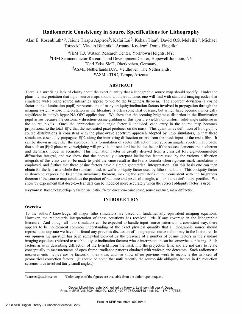
Figure 1† - Each Fourier order diffracted into the imaging system (assumed double telecentric here without loss of generality) constitutes a parallel bundle in object or image space whose width corresponds to an isoplanatic patch. Such bundles can be considered large compared to the lens resolution but small compared to the overall field size, and so can essentially be propagated through the lens as single rays. The areas cut by each Fourier bundle as it crosses the object and image planes must stand in the ratio of magnification squared, but the perpendicular cross-sections of the bundles vary over the pupil by an additional cosine factor. This gives rise to the so-called radiometric obliquity factor.

In deriving the obliquity factors for the imaging equations, the litho literature typically references classical treatments of scalar diffraction theory; by doing so the imaging equations can incorporate the cosinusoidal angular apodization factors (inclination or obliquity factors) that the classical diffraction theories predict. As we discuss below, the various diffraction formulations in the literature predict inclination factors that are (nominally) somewhat different.

Since these classical theories assume idealized thin-mask stencil screens (and in some cases Fresnel-type approximations in the geometry), it may not be immediately clear how applicable their inclination factors are to modern litho simulations involving e.g. hyper-NA and/or phase masks with thick multilayered topography. The question is one of practical importance since accurate OPC requires consideration of the detailed source shape1,2, and to address this need, state-of-the-art process models often include a measured tabulation of the intensity in the illumination pupil (or an accurate parametric representation). Moreover, as source design becomes more sophisticated it will be increasingly advantageous to employ precisely constructed source patterns of appreciable complexity3. In general, it is important that lithographic source maps provide the proper input to simulation tools, and that simulators properly interpret the source maps measured by exposure tools.

A key goal of this paper is to provide a definition of lithographic sources that is radiometrically valid, and that provides a correct prediction of image intensity (i.e. the |E|2 distribution within the resist film, which is a measure of the local resist reponse4). In addition, we will clarify the derivation of the various obliquity factors that arise in the standard imaging equations, and will provide intuitive explanations of their functional form. We will also demonstrate experimentally that measurements which include these factors provide appreciably better fits to measured intensities in resist (via dose to clear measurements).

Our goal is to provide a conceptually sound definition for the sources used in lithographic imaging models, but we will consider only the physical consistency of the underlying equations; numerical consistency is outside the scope of this paper. (We likewise ignore many practical issues of source metrology that must be considered once the conceptual definition is clearly established.) The radiometrically appropriate definition of the source that we derive is a new result, to our knowledge. The diffraction theory upon which it is based is certainly well-known, but we have tried to develop a more intuitive explanation of the cosine factors involved than we have

seen elsewhere. We will show that the obliquity factors involved in propagating from source to mask, and from mask to entrance pupil, both have common underpinnings - More specifically, they both describe the nonuniformity that arises in mapping direction cosine space to direction solid angle.

Generic imaging model in lithography Litho simulators use the input source description to set the magnitude E of the electric field illuminating the mask (as well as its state of polarization). To the best of our knowledge, all major simulators follow the equivalent of a more specific procedure appropriate to the Abbe model of image formation: User-input source maps are treated as a tabulation of the normalized |E|2 intensity of a gridded set of plane waves that illuminate the mask, or as a sampling in direction cosine space of the |E|2 produced by a continuous source. In many cases we have confirmed this both by querying the developers of these simulators, and by our own benchmark testing. Their choice of |E|2 for the source strength metric, instead of e.g. radiometric brightness (which would be an appropriate choice in a conventional

Proc. of SPIE Vol. 6924 69240V-2

0 0.2 0.4 0.6 0.80

1.0

2.0

0.5

1.5

2.5

a [at wafer]

Sour

ce E|

|2

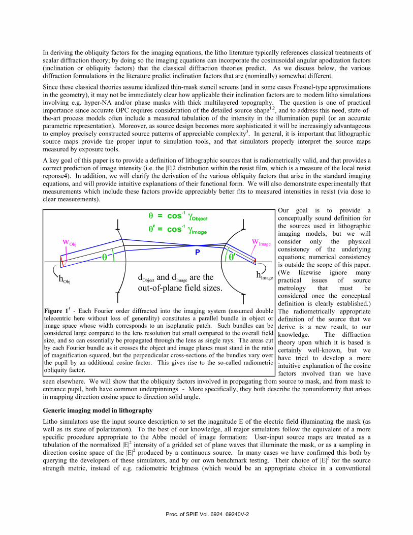
Figure 2† - Due to the eqs.[2] & [5] obliquity factor, a "tophat" source (red solid) that produces a uniform |E|2 out to some source radius (shown here as α=0.9) will produce a nonuniform |E|2 in the directional distribution illuminating the wafer (blue dashed). This example is for a non-immersion 4X system. |E|2 is calculated in air at both conjugates, it being assumed that thin-film models are used in a separate step to account for the effect of refraction into the resist layer, and into the mask blank. Lens transmission and the constant factor of magnification-squared are neglected in the plots.

radiometric measurement) affects the shape of the output image, as well as its dimensionality or overall scale. Of course, sources are conventionally supplied in normalized form, rather than in physical units (which for squared electric field might be e.g. [statvolt/cm]2), but even when normalized the interpretation of the source as proportional to |E|2 has influence on the shape of the calculated image. In fact, we show in section II that even a simple open frame intensity calculated by litho simulators would be in violation of the brightness invariance theorem (a fundamental physical result; see ref. 5) if the source intensity were interpreted as having standard radiometric units (i.e. brightness). For example, we will show that in the simple case of an imaging system for which the radiometric obliquity factor is unity, the open-frame wafer intensity |E|2 becomes independent of the radial distance at which a monopole test source (of specified size [in σ units] and intensity) is displaced from the optical axis, as long as the source intensity is interpreted as |E|2. However, we show that when source intensity is specified as a brightness measure, the open-frame intensity must instead change as the radial position of a fixed-brightness test source is made more oblique; this is a consequence of the brightness theorem, which states that the (index-scaled) source brightness must be the same in the object and image spaces (for an ideal lossless lens).

Sources are often tabulated in pupil coordinates (i.e. in "σ-space"), which, to within a constant of proportionality (NA), is the same as direction cosine space. In other cases the grid-step may be explicitly given in direction cosine units, e.g. as a step ∆αS, ∆βS (using here the conventional direction cosine notation, with subscript S denoting the source), meaning that the lS,mSth entry in an input source table supplies the intensity of the illuminating wave from a direction with k-vector

S Sk l ,m given by:

( )S S S S S S

2 20 0 S S S SS S S S Sˆ ˆ ˆ ˆk k , 1 ( ) ( ) ,k α x y z= = ∆α + ∆β + γ γ = − ∆α − ∆βl ,m l ,m l ,ml m l m [1]

where as usual 0k 2 ,≡ π λ z represents the optical axis, and lS and mS are integers whose range is determined by the maximum σ. Sometimes the source distribution is explicitly given in k-space; our assumption here is that the direction cosine space variables αS and βS are used. For concreteness we will assume that the αS, βS source coordinates refer to the propagation directions in air, rather than within the (typically SiO2) mask blank. However, in an accurate simulation it is necessary to consider the effect of refraction into the mask substrate, as discussed in section II.

Lithographic imaging models are ultimately grounded in the familiar Abbe model - In some cases the Abbe formulation is used explicitly, i.e. the partially coherent image is explicitly calculated as the incoherent sum of sub-images that are each coherently formed by an illuminating planewave from a particular source pixel (as in refs. 4,6,7), or the calculation may be carried out using the mutual coherence function (spatial domain), or TCC's (frequency domain), which essentially derive from the Abbe formulation by switching the order of integration/summation [so that the source integral precedes the integration(s) over the mask]. However, in all treatments that the authors are aware of (e.g. refs. 8-13), the source integration is carried out in the direction cosine units αS, βS of the eq.[1] grid (or in pupil coordinates where the direction cosines are simply scaled by a factor of NA), with the source intensities being treated as the square of the illuminating E-field. We also note that while most of our discussion is couched in terms of source inputs that are supplied in tabular form (per eq.[1]), our conclusions apply to any method that specifies the source as an |E|2 distribution in direction-cosine space (or in pupil coordinates).

The source tabulation is treated as applying to the mask plane illumination, though some simulators allow the overall image normalization to optionally be applied in the wafer space. It is natural under an Abbe model to employ a mask-plane normalization because the light in a given illuminating ray will typically arrive at the wafer along paths from many different pupil coordinates (having been split by diffraction at the mask). As will be discussed further below, the standard radiometric obliquity factor introduces a pupil-dependent

Proc. of SPIE Vol. 6924 69240V-3

Diffraction orders are uniformly spaced in direction cosine.

Spacing is non-uniform in solid angle.

∆α∆α/γ

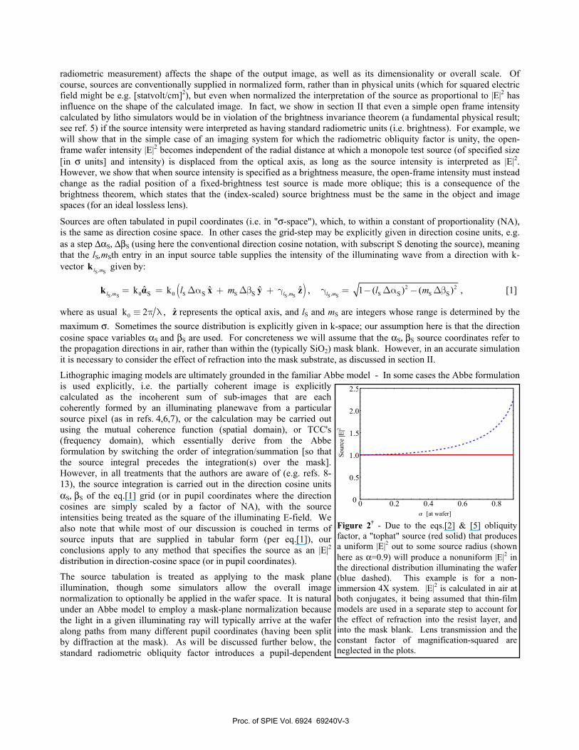
Figure 3† - When an object is illuminated by a source point that is focused into the pupil (shown here at a finite conjugate for simplicity), the directional distribution of the diffracted spectrum is uniform in cosine space, but nonuniform in solid angle. This follows from the grating law in the case of discrete orders (periodic boundary conditions), and the grid step between successive orders (which is constant in direction cosine units) subtends a solid angle that is increased by a factor 1/γ for orders that are steeply propagating. This can be understood to resultfrom foreshortening of the near-field spatial frequencies at steep obliquity.

apodization in E that is present even when the lens is ideal. This means that even in a mask-free open-frame exposure, a source having a classic tophat disk shape will not produce a tophat illuminating profile in the projection lens image space (Figure 2). As discussed further below, this has the implication that source brightness measurements should not be used directly as lithographic source inputs.

The interpretation of sources as |E|2 distributions is computationally appropriate under an Abbe model, since most steps of the detailed lens simulation involve the E-field, usually referring to the amplitude of planewaves. More generally, this "field-centric" representation is appropriate for the simulation of most aspects of the lithographic process. For example, rigorous E&M solvers that calculate the mask transmission use field variables, the Jones matrices that characterize the lens14 use the E field as input, as do the thin-film matrices that characterize the wafer process stack, and the resist response is likewise proportional to |E|2. Most simulators assume periodic boundary conditions on the mask, meaning that the Abbe orders are diffracted on a discrete grid in direction cosine space. A similar discrete gridding for integration might be used when TCCs are calculated. We note that interpolation may be necessary to mesh the grids of the illumination and collection pupils; however such numerical issues are generally outside the scope of this paper.

Similar issues of interpolation and anti-aliasing arise in simulating mask electromagnetic properties (so called EMF effects15). To account for large-angle effects in an accurate way it is necessary to make an accurate calculation of the mask transmission (using e.g. FDTD or RCWA [see ref. 16 for further background]), thereby obtaining the amplitudes of the Abbe imaging orders via Fourier transform of the E-field transmitted through each mask period (assuming periodic boundary conditions). Note that rigorous methods calculate mask "transmission" only in the formal sense of calculating the vector field at the output plane that is produced by a specified vector input. For practical efficiency one might stipulate that the detailed interactions of the illuminating fields with the mask topography entail only a slowly varying adjustment to

the ideal shift-invariant behavior of a generic thin mask (often referred to as Hopkins shift-invariance), allowing the fields diffracted from most of the discretely sampled source-waves to be obtained by interpolation across a limited number of mask simulations. We do not consider such computational questions in this paper. And while it is possible for reasons of computational efficiency to absorb certain limited departures of the mask behavior from pure shift invariance into an effective "optical" kernel12, we are concerned here with a conceptually accurate accounting of the imaging model, and do not consider this computational shortcut which in effect blurs the division between mask and lens. (We likewise ignore the computational advantages gained by absorbing resist diffusion and film stack effects into the optical kernel.)

Obliquity factor Litho simulators apply a so-called radiometric obliquity factor to the individual Abbe plane wave components. To the authors' knowledge it was Richards and Wolf17 who first recognized the need for this radiometric correction. Though the basic Abbe model is essentially angular-spectrum-based, most published derivations of the obliquity factor obtain it through application of classical diffraction theory to three separate stages of propagation through the lens (see for example ref. 4), in order to take into account the apodizing inclination factor that arises in diffracting from the mask to the entrance pupil:

Proc. of SPIE Vol. 6924 69240V-4

Light

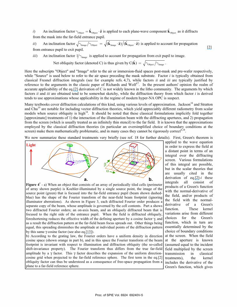
a. b.Figure 4† - a) When an object that consists of an array of periodically tiled cells (perimeter of array shown purple) is Koehler-illuminated by a single source point, the image of the source point (green) that is focused into the far-field entrance pupil (beam shown dashed-blue) has the shape of the Fourier transform of the near-field beam footprint (ignoring illuminator aberrations). As shown in Figure 3, each diffracted Fourier order produces a separate copy of the beam, whose amplitude is governed by the cell contents. Part a shows two diffracted Fourier orders; an on-axis beam, and an obliquely diffracted beam that is focused to the right side of the entrance pupil. When the field is diffracted obliquely, foreshortening reduces the effective width of the defining aperture by a cosine factor γ, and as a result the diffraction pattern at the far-field beam focus spreads out. Other things being equal, this spreading diminishes the amplitude at individual points of the diffraction pattern by this same γ cosine factor (see also eq.[13]). b) According to the grating law, the Fourier orders have a uniform density in direction cosine space (shown orange in part b), and in this space the Fourier transform of the beam footprint is invariant with respect to illumination and diffraction obliquity (the so-called shift-invariance property). The Fourier transform thus differs from the true far-field amplitude by a γ factor. This γ factor describes the expansion of the uniform direction-cosine grid when projected to the far-field reference sphere. The first term in the eq.[2]obliquity factor can thus be understood as a consequence of free-space propagation from a plane to a far-field reference sphere.

Object Object Object

Image Object Im

ˆ ˆˆ) An inclination factor is applied to each plane-wave component as it diffractsfrom the mask into the far-field entrance pupil.

ˆ) An inclination factor (

γ = ⋅

γ γ =

k z k

k

i

ii age Object

Image

ˆˆ ˆ) ( ) is applied to account for propagationfrom entrance pupil to exit pupil.

) An inclination factor 1 is applied to account for propagation from exit pupil to image.

Net obliqui

⋅ ⋅

γ

z k z

iii

Object Imageˆty factor (denoted C) is thus given by C( ) .= γ γk

[2]

Here the subscripts "Object" and "Image" refer to the air or immersion-fluid spaces post-mask and pre-wafer respectively, while "Source" is used below to refer to the air space preceding the mask substrate. Factor i is typically obtained from classical Fresnel diffraction integrals (see for example refs. 4,7), while factors ii and iii are typically justified by reference to the arguments in the classic paper of Richards and Wolf17. In the present authors' opinion the realm of accurate applicability of the eq.[2] derivation of C is not widely known in the litho community. The arguments by which factors ii and iii are obtained tend to be somewhat sketchy, while the diffraction theory from which factor i is derived tends to use approximations whose applicability in the regime of modern hyper-NA OPC is suspect.

Many textbooks cover diffraction calculations of this kind, using various levels of approximation. Jackson18 and Stratton and Chu19 are notable for including vector diffraction theories, which yield appreciably different radiometry from scalar models when source obliquity is high18. It should be noted that these classical formulations implicitly fold together [approximate] treatments of 1) the interaction of the illumination beam with the diffracting apertures, and 2) propagation from the screen (which is usually treated as an infinitely thin stencil) to the far field. It is known that the approximations employed by the classical diffraction theories (in particular an oversimplified choice of boundary conditions at the screen) make them mathematically problematic, and in many cases they cannot be rigorously correct8,18.

We now summarize these standard treatments very briefly (see ref. 18 for further details). First, Green's theorem is applied to the wave equation in order to express the field at a distant point in terms of an integral over the diffracting screen. Various formulations of this integral are possible, but in the scalar theories that are usually cited in the derivation of eq.[2]-i these integrals all consist of products of a Green's function with the normal-derivative of the field, and/or products of the field with the normal-derivative of a Green's function. These kernel variations arise from different choices for the Green's function, which in turn are essentially determined by the choice of boundary conditions at the screen. When the field at the aperture is known (assumed equal to the incident field multiplied by the screen transmission in classical treatments), the kernel includes the derivative of the Green's function, which gives

Proc. of SPIE Vol. 6924 69240V-5

rise in the far-field to the γObject inclination factor i in eq.[2]. (The associated scalar diffraction integral is known as the Rayleigh-Sommerfeld integral with Dirichlet boundary conditions.) However, one can instead assume that the known quantity at the screen is the derivative of the field in the outward-normal direction. Classically, this quantity is assumed to be equal to the derivative of the incident field (within the open screen apertures). With this second choice of boundary conditions the classical formulations arrive at an inclination factor of γSource (Rayleigh-Sommerfeld with Neumann boundary conditions). Alternatively, by using the simplest choice of boundary conditions (which, however, gives rise in the classical treatments to the most severe mathematical inconsistencies) one arrives at the Kirchoff formulation, in which the inclination factor is (γObject + γSource)/2.

In the far-field all of these scalar formulations differ only in their obliquity factor. Though the Kirchoff boundary conditions are the most problematic mathematically18, the Kirchoff obliquity factor has intuitive plausibility in registering an effect from inclination of either the source or collection directions. And in point of fact all of these boundary conditions are known to be mathematically invalid unless the field exhibits a singularity along the aperture edges8, in the case of the idealized perforated screens (infinitely conductive and infinitely thin) that are assumed in the classical theory. This difficulty seemingly calls into question the accuracy of any of the standard choices for the obliquity factor that might be used in item i of eq.[2], and of course today's lithographic masks bear little resemblance to the idealized classical apertures.

However, it is not widely appreciated that all of these formulations can readily be made consistent and rigorous if the fields are accurately known at the exit of the screen/mask, a point we discuss in detail in the next section. (See also Kerwien et al.20) We then show that an appropriate reformulation is already implicitly incorporated into the standard Abbe model used by litho simulators, with one qualification - It appears not to have been explicitly recognized before now that in order to properly calculate the correct |E|2 distribution within the resist, such simulators must be provided with a source map that is proportional to the product of source radiance (brightness) and pixel solid angle, the latter factor being essentially equivalent to a 1/γSource apodization.

Before turning to these topics we should note that the literature includes a derivation of the eq.[2] obliquity factor which is quite different from that described above. Gallatin21 derives the obliquity factor by applying an energy conservation expression for scalar fields to the case of high-NA scalar imaging. A more intuitive derivation along the same lines (which applies equally well in the vector-imaging case) had previously been made in ref. 6, and was later elaborated in ref. 22; we now summarize it here.

For purposes of discussion we can analyze the imaging radiometry by considering a mask region that covers a single isoplanatic patch (i.e. a region of uniform imaging), and in a high-quality imaging application we can assume the isoplanatic patch to be many times larger than the object period. This is illustrated in Figure 1. Under illumination by a single source point, each Fourier order will diffract from the isoplanatic patch as a bundle of rays that is converged through a common point P in the pupil. (In fact the bundle forms a diffraction pattern at point P corresponding to the Fourier transform of the beam aperture, as we discuss later.) Energy conservation and Poynting's theorem require that the total power in the bundle satisfy

2 2Image Lens Object(n A E ) T (n A E ) where A w d.= ≡⊥ ⊥ ⊥ [3]

Here n represents the refractive index, in object space or image space. (We define the image space as the coupling medium immediately above the wafer; the effect of refraction into the resist layer is assumed to be dealt with separately via a thin-film calculation4.) TLens is the intensity transmission of the lens, E is the electric field, w the perpendicular cross-section of the bundle in the plane of the Figure 1 diagram, and d the out-of-plane cross-section. The oblique (non-perpendicular) cross-sections of the bundle as taken across the object and image planes must stand in the fixed ratio of the lens magnification (which we will denote as M), and as a result the perpendicular cross-section A⊥ will vary with diffracted direction. Thus, letting h denote the (oblique, non-perpendicular) span of the beam boundaries as cut by the object or image planes, we have Image Image Image Object Object Object Image Object Image Objectw h , w h , h Mh , d Md .= γ = γ = = [4]

Eqs.[3] and [4] then yield the following expression for the obliquity factor C:

Object Object ObjectLens

Image Image Image

Image

Object

n1T

M n

EC (Usually only the cosine factors are retained.)

Eγ γ

γ γ≡ = ∝ [5]

Proc. of SPIE Vol. 6924 69240V-6

The obliquity factor arises automatically in any moderately well-corrected lens when the Fourier orders are reconverged with rescaled direction cosines in order to create a demagnified image. Through very similar arguments we show in section II that this process maintains the brightness theorem. We first show in section I that such geometrical considerations also underlie the diffraction-based inclination factor in eq.[2]-i. When employing the eq.[2] line of argument one might question whether a Rayleigh-Sommerfeld (Dirichlet) inclination factor is applicable in modern high-NA vector imaging simulations. For example, in critical cases where rigorous mask EMF simulations are carried out, use of an obliquity factor from Rayleigh-Sommerfeld scalar diffraction theory appears to mix exact and approximate diffraction calculations. We show below that these approaches are in fact quite consistent.

I. INCLINATION FACTOR IN MASK DIFFRACTION

Inclination factor in the plane wave spectrum The angular spectrum approach to diffraction theory can be derived directly from Maxwell's equations23, and is a well-known framework for analyzing imaging systems24. In an angular spectrum treatment one can use the arguments of refs. 6,21,22 (summarized in Figure 1 and eqs.[3]-[5] above) to derive the obliquity factor. However, in order to clarify the connection between this approach and the more prevalent diffraction-based treatment summarized as eq.[2] above, we show in an Appendix that the rigorous Franz vector diffraction formula reproduces the angular spectrum result used by litho simulators. The Franz formula is regarded as the most rigorous of the standard vector diffraction formulations (see ref. 25, and also ref. 26), in that other vector diffraction formulae require the addition of ad hoc edge terms when used with classical boundary conditions. A key point, however, is that in free space all of these vector formulations are equivalent (see the Appendix). By using a Maxwell solver to numerically propagate the illuminating fields to the output face of the mask, the analytical problem faced by litho simulators in carrying out the eq.[2]-i propagation from mask to entrance pupil is greatly eased. In particular, we show in the Appendix that as long as the mask exit plane is offset by a finite distance from the mask topography, the Franz formula will simply reproduce the angular spectrum result. More specifically, the Appendix shows that if we begin by formally calculating the local angular spectrum as a mathematical 2D Fourier transform of the field at the mask exit plane z = zM, i.e. if we represent this field by

( ) ( ) ( ) ( ) M M M Mx y

M

2D Inverse Fourier Transform

j1 or dk dk , z or , z e ,2≡

π ∫∫k rE r H r k kE H ⋅ [6]

with tildes denoting 2D vectors in the x,y plane, then Maxwell's equations imply that

( ) ( )M M0k , z , z ,= ×k k kE H [7]

and the Franz formula for the fields in a further-distant plane z = zP reduces upon Fourier transformation to the angular spectrum result

( ) ( ) ( ) ( ) P M0P P M M jk (z z ), z or , z , z or , z e .k k k k γ −=E H E H [8]

The 2D forward-transform that inverts eq.[6] is

( ) ( ) j1, z dxdy , z e .2

k rk E r −=π ∫∫E ⋅ [9]

Evaluating this in the zP and zM planes, and substituting into eq.[8], we find from the identity 0k zk r k r⋅ ≡ ⋅ + γ :

( ) ( ) ( ) ( ) PP Px y

j1 or dk dk ,0 or , 0 e ,2

k rE r H r k k ⋅=π ∫∫ E H [10]

indicating that the 2D Fourier components of the field in fact propagate in 3D as plane waves. We should note a subtlety in the notation used here: We have written the field Fourier amplitudes with a script font to indicate their calculation via a simple 2D Fourier transform over a plane, i.e. eq.[6] implicitly defines them by a purely mathematical or numerical operation whose equivalence to planewave decomposition is derived rather than presumed. This transformation is two-dimensional, i.e. over x and y (or kx and ky in the inverse transform), which we indicate using a tilde over the

Proc. of SPIE Vol. 6924 69240V-7

corresponding vector variable, e.g. x y 0ˆ ˆ ˆ ˆk k k ( )≡ + = α + βk x y x y , where as usual the direction cosines of the full 3D

propagation vector k are denoted α,β,γ, so that 0 ˆk= + γk k z . These 2D transforms do not involve any adjustments in z or kz; however the eq.[10] result from the Franz formula shows that the Fourier components do in fact propagate along z as plane waves. (This fundamental angular spectrum result is usually obtained directly from Maxwell's equations, and can in fact be used as a basis for deriving the Franz formula [reversing the procedure of the last two paragraphs; see Appendix], under the free-space conditions in which there are no currents or back-propagated waves between the mask exit plane and the far field.)

Eq.[10] applies no obliquity factor to the Fourier order, and thus may appear inconsistent with factor i of eq.[2]. As discussed above, factor i arises during propagation to the far-field (entrance pupil), and is the first of a sequence of terms in eq.[2] which together comprise the radiometric obliquity factor. However, propagation to the far-field is not precisely equivalent to plane-wave propagation. Though this point may be seen by close reading of the literature, it is not explicitly explained in the treatments known to the authors. In order to provide an intuitively clear explanation, we make use of a lemma of Jones27, cited by Alonso and Borghi28, which states the mathematical result that when a vector field F can be represented as a distribution A over a set of plane waves that are uniformly dense in direction, i.e.

0

ForwardSolidAngle

jk ˆˆ( ) d ( )e ,w rF r A w ⋅= Ω∫ [11]

we find that at a large distance R from the origin 0(Rk 1), the field will asymptotically approach the far-field value

0jk Reˆ ˆ(R ) ( ) ,

j(R )≅

λF r A r [12]

where we have assumed all waves to be forward-traveling. Eq.[12] states the intuitively plausible result that when the planewave components are uniformly distributed in solid angle Ω, the field that propagates outward in some direction r will become equal to the amplitude of the particular planewave component ˆ( )A r which is propagating in that same direction, phase-shifted across the propagation distance (with additional π/2 quadrature phase shift), and attenuated with a 1/R2 intensity scaling. Note that the eq.[12] result contains no obliquity factor. However, eq.[12] is based on the eq.[11] expansion over a planewave basis that is directionally uniform, i.e. uniform in direction solid angle. In contrast, the grating law implies that the planewave spectrum diffracted from a planar mask will be uniformly dense in direction-cosine space, not direction solid angle. Equi-spacing in direction-cosine simply expresses the elementary requirement that the oscillation across the unit cell x y(e.g. of periodicity p ,p ) must increment by one cycle between successive diffraction orders, in order that the spatial frequency harmonics of the near-field be matched by the oscillation along cross-sections of the diffracted planewaves. Foreshortening of these spatial frequencies implies a non-constant angular step between adjacent orders (for diffraction angles outside the paraxial regime). Quantitatively, each uniform step in direction cosine (denoted ,∆α ∆β , with

x y, / p , / p∆α ∆β ≡ λ λ ) will subtend a solid angle that varies over the pupil according to (see Figure 3):

2 2

( , ) .1

∆α∆β ∆α∆β∆Ω α β = =

γ −α −β [13]

If we now use eq.[13] to substitute 2 2x y 0 0dk dk k d d k d= α β= γ Ω into eq.[10], and apply the eqs.[11] and [12]

asymptotic identity with A set to ,γE rP set to ˆR ,α and with F set to P( ),E r we obtain for the far-field amplitude:

( )0jk R

ObjectFarField

eˆ(R ) ,0 ,jR

= γE α kE [14]

which now includes an obliquity factor (specifically factor i of eq.[2], traditionally obtained from the Rayleigh-Sommerfeld [Dirichlet] diffraction integral). We have given γ the subscript "Object" to emphasize that it refers to the

Proc. of SPIE Vol. 6924 69240V-8

propagation angle (against z) in the object space between mask and entrance pupil. In a similar way γSource denotes the inclination of a planewave component illuminating the mask, and γImage the inclination of a planewave illuminating the wafer. (Note that the above discussion assumes periodic boundary conditions and a discrete spectrum for purposes of discussion, but is in fact quite general.)

The inclination factor in eq.[14] that multiplies the planewave amplitude is seen to arise from the decreased density of the angular spectrum at high obliquity. We show in the next subsection that this is essentially a foreshortening effect. We can put eq.[14] in conventional Fraunhofer-like form by using eq.[8] to back-propagate to the origin, i.e. setting

( ) ( ) 0MM jk z,0 , z e ,k k γ−=E E [15]

and then applying eq.[9] at z = zM to obtain from eq.[14] M M ˆ(using z):≡ + γr r

0jk R

MM MObject

FarField

M0ˆjkeˆ(R ) dx dy ( ) e ,

jR−

= γ ∫∫α rE α E r ⋅ [16]

which is the standard Fraunhofer result, containing the usual obliquity factor γObject.

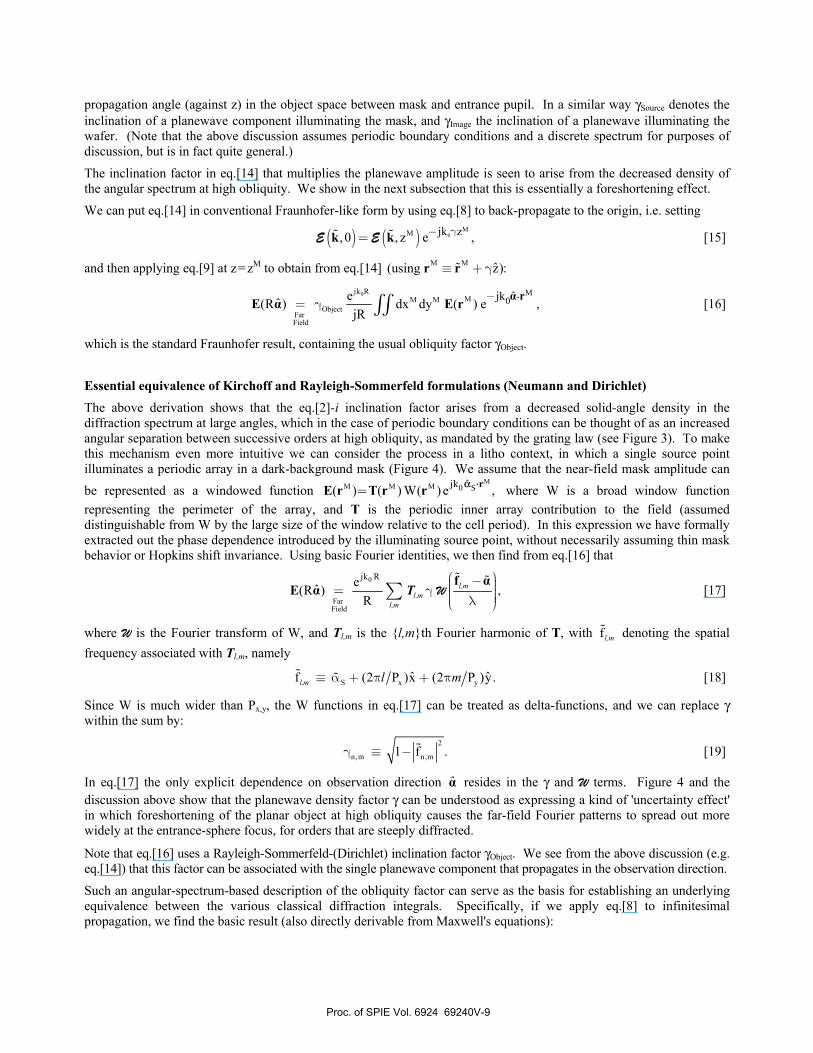
Essential equivalence of Kirchoff and Rayleigh-Sommerfeld formulations (Neumann and Dirichlet) The above derivation shows that the eq.[2]-i inclination factor arises from a decreased solid-angle density in the diffraction spectrum at large angles, which in the case of periodic boundary conditions can be thought of as an increased angular separation between successive orders at high obliquity, as mandated by the grating law (see Figure 3). To make this mechanism even more intuitive we can consider the process in a litho context, in which a single source point illuminates a periodic array in a dark-background mask (Figure 4). We assume that the near-field mask amplitude can be represented as a windowed function

MM M M 0 Sˆjk( ) ( ) W( ) e ,rE r T r r ⋅= α where W is a broad window function

representing the perimeter of the array, and T is the periodic inner array contribution to the field (assumed distinguishable from W by the large size of the window relative to the cell period). In this expression we have formally extracted out the phase dependence introduced by the illuminating source point, without necessarily assuming thin mask behavior or Hopkins shift invariance. Using basic Fourier identities, we then find from eq.[16] that

0

FarField

jk Reˆ(R ) ,R

⎛ ⎞− ⎟⎜ ⎟⎜= γ ⎟⎜ ⎟⎟⎜ λ⎝ ⎠∑

f αE α WT l,m

l,ml,m

[17]

where W is the Fourier transform of W, and Tl,m is the l,mth Fourier harmonic of T, with fl,m denoting the spatial frequency associated with Tl,m, namely

S x yˆ ˆf (2 P )x (2 P )y.≡ α + π + πl,m l m [18]

Since W is much wider than Px,y, the W functions in eq.[17] can be treated as delta-functions, and we can replace γ within the sum by:

2

n,m n,m1 f .γ ≡ − [19]

In eq.[17] the only explicit dependence on observation direction α resides in the γ and W terms. Figure 4 and the discussion above show that the planewave density factor γ can be understood as expressing a kind of 'uncertainty effect' in which foreshortening of the planar object at high obliquity causes the far-field Fourier patterns to spread out more widely at the entrance-sphere focus, for orders that are steeply diffracted.

Note that eq.[16] uses a Rayleigh-Sommerfeld-(Dirichlet) inclination factor γObject. We see from the above discussion (e.g. eq.[14]) that this factor can be associated with the single planewave component that propagates in the observation direction. Such an angular-spectrum-based description of the obliquity factor can serve as the basis for establishing an underlying equivalence between the various classical diffraction integrals. Specifically, if we apply eq.[8] to infinitesimal propagation, we find the basic result (also directly derivable from Maxwell's equations):

Proc. of SPIE Vol. 6924 69240V-9

Measured vs. Simulated E0

0

2

4

6

8

10

12

0.5 0.6 0.7 0.8 0.9σcenter

E0 (m

J/cm

2)

with Obliquity

E0_meas

without Obliquity

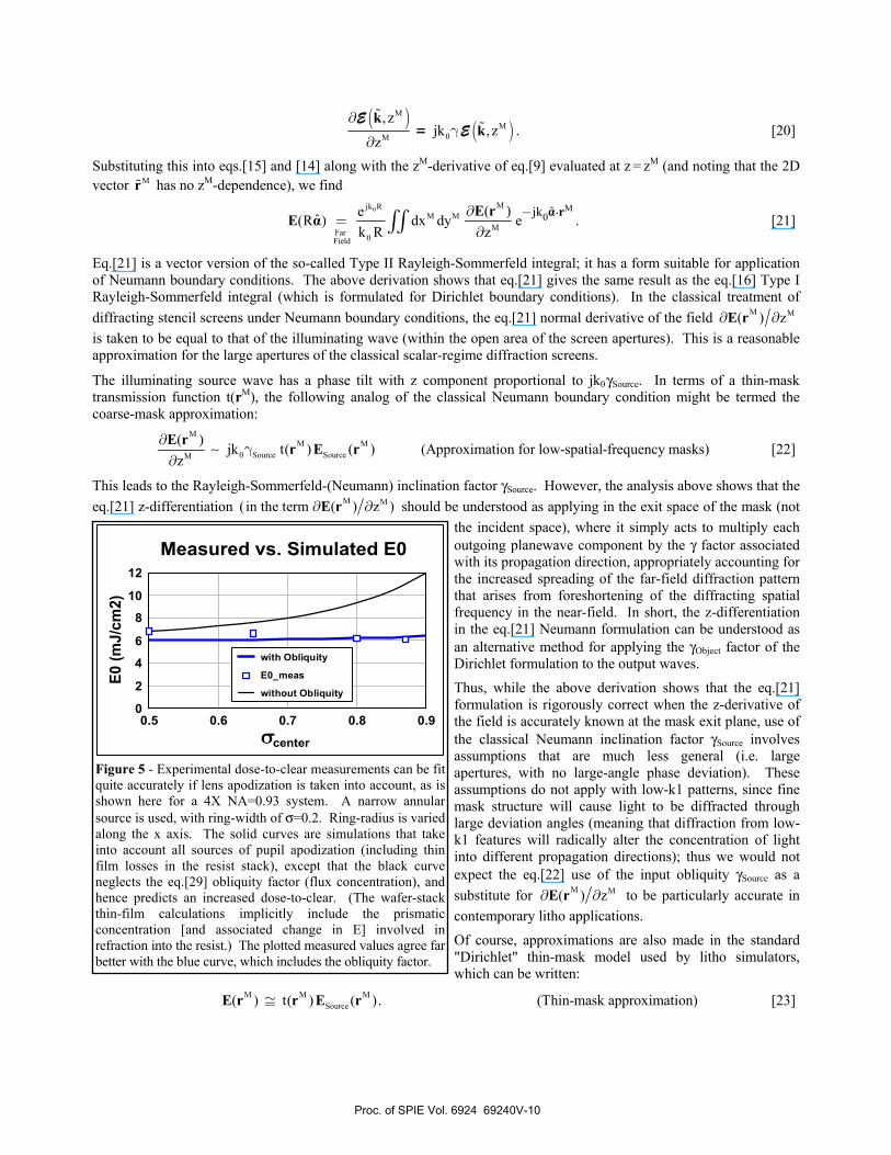
Figure 5 - Experimental dose-to-clear measurements can be fit quite accurately if lens apodization is taken into account, as is shown here for a 4X NA=0.93 system. A narrow annular source is used, with ring-width of σ=0.2. Ring-radius is varied along the x axis. The solid curves are simulations that take into account all sources of pupil apodization (including thin film losses in the resist stack), except that the black curve neglects the eq.[29] obliquity factor (flux concentration), and hence predicts an increased dose-to-clear. (The wafer-stack thin-film calculations implicitly include the prismatic concentration [and associated change in E] involved in refraction into the resist.) The plotted measured values agree far better with the blue curve, which includes the obliquity factor.

( )

( )M

M0M

, zjk , z .

z

∂γ

∂

kk

E= E [20]

Substituting this into eqs.[15] and [14] along with the zM-derivative of eq.[9] evaluated at z = zM (and noting that the 2D vector Mr has no zM-dependence), we find

0 Mjk R

M MMFar 0Field

M0 ˆjk( )eˆ(R ) dx dy e .

k R z−∂

=∂∫∫

α rE rE α ⋅ [21]

Eq.[21] is a vector version of the so-called Type II Rayleigh-Sommerfeld integral; it has a form suitable for application of Neumann boundary conditions. The above derivation shows that eq.[21] gives the same result as the eq.[16] Type I Rayleigh-Sommerfeld integral (which is formulated for Dirichlet boundary conditions). In the classical treatment of diffracting stencil screens under Neumann boundary conditions, the eq.[21] normal derivative of the field M M( ) z∂ ∂E r is taken to be equal to that of the illuminating wave (within the open area of the screen apertures). This is a reasonable approximation for the large apertures of the classical scalar-regime diffraction screens.

The illuminating source wave has a phase tilt with z component proportional to jk0 γSource. In terms of a thin-mask transmission function t(rM), the following analog of the classical Neumann boundary condition might be termed the coarse-mask approximation:

M

M M0 Source SourceM

( )jk t( ) ( ) (Approximation for low-spatial-frequency masks)

z∂

γ∂E r

r E r∼ [22]

This leads to the Rayleigh-Sommerfeld-(Neumann) inclination factor γSource. However, the analysis above shows that the eq.[21] z-differentiation M M(in the term ( ) z )∂ ∂E r should be understood as applying in the exit space of the mask (not

the incident space), where it simply acts to multiply each outgoing planewave component by the γ factor associated with its propagation direction, appropriately accounting for the increased spreading of the far-field diffraction pattern that arises from foreshortening of the diffracting spatial frequency in the near-field. In short, the z-differentiation in the eq.[21] Neumann formulation can be understood as an alternative method for applying the γObject factor of the Dirichlet formulation to the output waves. Thus, while the above derivation shows that the eq.[21] formulation is rigorously correct when the z-derivative of the field is accurately known at the mask exit plane, use of the classical Neumann inclination factor γSource involves assumptions that are much less general (i.e. large apertures, with no large-angle phase deviation). These assumptions do not apply with low-k1 patterns, since fine mask structure will cause light to be diffracted through large deviation angles (meaning that diffraction from low-k1 features will radically alter the concentration of light into different propagation directions); thus we would not expect the eq.[22] use of the input obliquity γSource as a substitute for M M( ) z∂ ∂E r to be particularly accurate in contemporary litho applications. Of course, approximations are also made in the standard "Dirichlet" thin-mask model used by litho simulators, which can be written:

M M MSource( ) t( ) ( ). (Thin-mask approximation)E r r E r≅ [23]

Proc. of SPIE Vol. 6924 69240V-10

θ = cos-1 gObject

θ' = cos-1 gImage

θ θ'

hImagehObj

( )∆α ∆β, ObjectS S ( )∆α ∆βS, ImageS

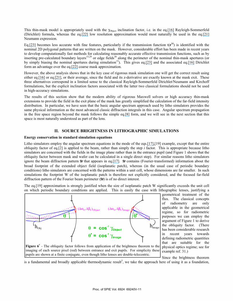
Figure 6† - The obliquity factor follows from application of the brightness theorem to the imaging of each source pixel (red) between entrance and exit pupils. For simplicity these pupils are shown at a finite conjugate, even though litho lenses are double-telecentric.

This thin-mask model is appropriately used with the γObject inclination factor, i.e. in the eq.[16] Rayleigh-Sommerfeld (Dirichlet) formula, whereas the eq.[22] low resolution approximation would most naturally be used in the eq.[21] Neumann expression. Eq.[23] becomes less accurate with fine features, particularly if the transmission function t(rM) is identified with the nominal 2D polygonal patterns that are written on the mask. However, considerable effort has been made in recent years to develop computationally fast methods for calculating reasonably accurate effective transmission functions, such as by inserting pre-calculated boundary layers15,29 or edge fields30 along the perimeter of the nominal thin-mask apertures (or by simply biasing the nominal apertures during simulation15). This gives eq.[23] and the associated eq.[16] Dirichlet form an advantage over the eq.[22] coarse mask approximation. However, the above analysis shows that in the key case of rigorous mask simulation one will get the correct result using either eq.[16] or eq.[21], or their average, since the field and its z-derivative are exactly known at the mask exit. These three alternatives correspond in a limited sense to the classical Rayleigh-Sommerfeld Dirichlet/Neumann and Kirchoff formulations, but the explicit inclination factors associated with the latter two classical formulations should not be used in high-accuracy simulations. The results of this section show that the modern ability of rigorous Maxwell solvers or high accuracy thin-mask extensions to provide the field in the exit plane of the mask has greatly simplified the calculation of the far-field intensity distribution. In particular, we have seen that the basic angular spectrum approach used by litho simulators provides the same physical information as the most advanced classic diffraction integrals in this case. Angular spectrum propagation in the free space region beyond the mask follows the simple eq.[8] form, and we will see in the next section that this space is most naturally understood as part of the lens.

II. SOURCE BRIGHTNESS IN LITHOGRAPHIC SIMULATIONS Energy conservation in standard simulation equations Litho simulators employ the angular spectrum equations in the mode of the eqs.[17],[19] example, except that the entire obliquity factor of eq.[2] is applied to the beam, rather than simply the step i factor. This is appropriate because litho simulators are concerned with the fields in the image plane rather than in the entrance pupil (and Figure 1 shows that the obliquity factor between mask and wafer can be calculated in a single direct step). For similar reasons litho simulators ignore the beam diffraction pattern W that appears in eq.[17]. W contains (Fourier-transformed) information about the broad footprint of the extended object field (isoplanatic patch), whereas (in the usual case of periodic boundary conditions) litho simulators are concerned with the patterns within a unit cell, whose dimensions are far smaller. In such simulations the footprint W of the isoplanatic patch is therefore not explicitly considered, and the focused far-field diffraction pattern of the Fourier beam perimeter (W) is of no direct interest.

The eq.[19] approximation is strongly justified when the size of isoplanatic patch W significantly exceeds the unit cell on which periodic boundary conditions are applied. This is easily the case with lithographic lenses, justifying a

geometrical treatment of the flux. The classical concepts of radiometry are only applicable in the geometrical regime, so for radiometric purposes we can employ the argument of Figure 1 to derive the obliquity factor. (There has been considerable research in recent years towards defining radiometric quantities that are suitable for the physical optics regime; see for example ref. 31.) Since the brightness theorem

is a fundamental and broadly applicable thermodynamic result5, we take the approach here of using it as a foundation,

Proc. of SPIE Vol. 6924 69240V-11

LightPixels at large radii in direction cosine space subtend larger solid angles.

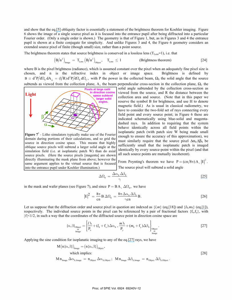
Figure 7† - Litho simulators typically make use of the Fourier domain during portions of their calculations, and so grid the source in direction cosine space. This means that highly oblique source pixels will subtend a larger solid angle at the simulation field (i.e. at isoplanatic patch W) than do axial source pixels. (Here the source pixels [magenta] are shown directly illuminating the mask plane from above; however the same argument applies to the virtual source that is focused into the entrance pupil under Koehler illumination.)

and show that the eq.[5] obliquity factor is essentially a statement of the brightness theorem for Koehler imaging. Figure 6 shows the image of a single source pixel as it is focused into the entrance pupil after being diffracted into a particular Fourier order. (Only a single order is shown.) The geometry is that of Figure 1, but, as in Figures 3 and 4 the entrance pupil is shown at a finite conjugate for simplicity. And unlike Figures 3 and 4, the Figure 6 geometry considers an extended source pixel of finite (though small) size, rather than a point source. The brightness theorem states that source brightness is conserved in a lossless lens (TLens=1), i.e. that

( ) ( )2 2Lens LensImage Object

B n T B n , T 1 (Brightness theorem)= ≤ [24]

where B is the pixel brightness (radiance), which is assumed constant over the pixel when an adequately fine pixel size is chosen, and n is the refractive index in object or image space. Brightness is defined by

2 2S S CB ( )d P d dA 1 R d P d d ,≡ =Ω Ω Ω⊥ with P the power in the collected beam, ΩS the solid angle that the source

subtends as viewed from the collection plane, A⊥ the beam perpendicular cross-section in the collection plane, ΩC the solid angle subtended by the collection cross-section as viewed from the source, and R the distance between the collection area and source. (Note that in this paper we reserve the symbol B for brightness, and use H to denote magnetic field.) As is usual in classical radiometry, we have to consider the two-fold set of rays connecting every field point and every source point; in Figure 6 these are indicated schematically using blue-solid and magenta-dashed rays. In addition to requiring that the system behave identically across all field points within the isoplanatic patch (with patch size W being made small enough to ensure the accuracy of this approximation), we must similarly require that the source pixel ∆αS ∆βS be sufficiently small that the isoplanatic patch is imaged identically by every source-point within the pixel (and that all such source points are mutually incoherent).

From Poynting's theorem we have 2P (cn 8 ) A E .⊥= π The source pixel will subtend a solid angle

S SS

∆α ∆β∆Ω =

γ [25]

in the mask and wafer planes (see Figure 7), and since SP BA ,⊥= ∆Ω we have

S SS

882E B B.cn cn

π∆α ∆βπ= ∆Ω =

γ [26]

Let us suppose that the diffraction order and source pixel in question are indexed as l,m (eq.[18]) and lS,mS (eq.[1]), respectively. The individual source points in the pixel can be referenced by a pair of fractional factors fx,fy, with | f |<1/2, in such a way that the coordinates of the diffracted source point in direction cosine space are

Object S x S S y SObjector x y orImageImage

, ( f ) , ( f ) .P P

⎧ ⎫⎪ ⎪λ λ⎪ ⎪α β = + + ∆α + + ∆β⎨ ⎬⎪ ⎪⎪ ⎪⎩ ⎭

l ml m [27]

Applying the sine condition for isoplanatic imaging to any of the eq.[27] rays, we have

( ) ( )Image Object

Image S, Image Object S,Object Image S, Image Object S,Object

M n , n , ,

which implies:M n n ; M n n .

α β = α β

∆α = ∆α ∆β = ∆β [28]

Proc. of SPIE Vol. 6924 69240V-12

(The sine condition simply expresses the requirement that any interfering set of spatial frequencies in the object reproduce the same interference pattern in the image at the reduced scale dictated by magnification M.) If we now substitute eqs.[28] and [26] into the brightness theorem (eq.[24]), we recover the eq.[5] expression for the obliquity factor C:

Object ObjectLens

Image Image

Image

Object

n1T

M n

EC .

Eγ

γ≡ = [29]

Eq.[29] describes the cumulative effect of beam refraction across all surfaces in the projection lens. It does not include the effect of refraction into the resist film. (Recall that the refractive index nImage appearing in eq.[29] is the index of the air or immersion fluid adjacent to the wafer.) To properly account for vector imaging effects it is necessary to propagate the waves into the resist layer, and this can be accomplished using a thin-film model of the resist stack4, for which eq.[29] properly corrects the incident field.

We also note that in an open frame exposure the transfer equation Image ImageObject Object22E E∝ γ γ used by litho

simulators and the similar equation Image Image2E B∝ γ involving source brightness predict different numerical outputs

when a source pole of constant numerical input intensity Object2

( E versus B) is translated in the pupil, except in the

limit where the object-side NA is small. This means that if measured source brightness is used as an input to a litho

simulator instead of Object2

E , the output image intensity cannot be radiometrically correct. We will return to this point

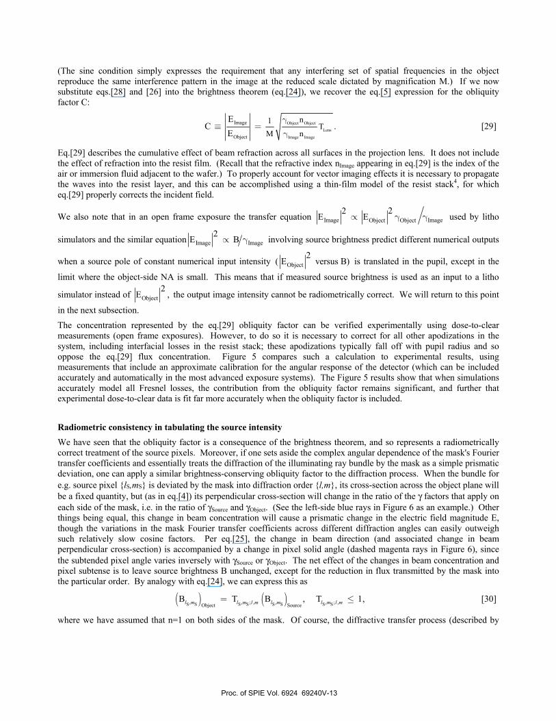
in the next subsection. The concentration represented by the eq.[29] obliquity factor can be verified experimentally using dose-to-clear measurements (open frame exposures). However, to do so it is necessary to correct for all other apodizations in the system, including interfacial losses in the resist stack; these apodizations typically fall off with pupil radius and so oppose the eq.[29] flux concentration. Figure 5 compares such a calculation to experimental results, using measurements that include an approximate calibration for the angular response of the detector (which can be included accurately and automatically in the most advanced exposure systems). The Figure 5 results show that when simulations accurately model all Fresnel losses, the contribution from the obliquity factor remains significant, and further that experimental dose-to-clear data is fit far more accurately when the obliquity factor is included.

Radiometric consistency in tabulating the source intensity We have seen that the obliquity factor is a consequence of the brightness theorem, and so represents a radiometrically correct treatment of the source pixels. Moreover, if one sets aside the complex angular dependence of the mask's Fourier transfer coefficients and essentially treats the diffraction of the illuminating ray bundle by the mask as a simple prismatic deviation, one can apply a similar brightness-conserving obliquity factor to the diffraction process. When the bundle for e.g. source pixel lS,mS is deviated by the mask into diffraction order l,m, its cross-section across the object plane will be a fixed quantity, but (as in eq.[4]) its perpendicular cross-section will change in the ratio of the γ factors that apply on each side of the mask, i.e. in the ratio of γSource and γObject. (See the left-side blue rays in Figure 6 as an example.) Other things being equal, this change in beam concentration will cause a prismatic change in the electric field magnitude E, though the variations in the mask Fourier transfer coefficients across different diffraction angles can easily outweigh such relatively slow cosine factors. Per eq.[25], the change in beam direction (and associated change in beam perpendicular cross-section) is accompanied by a change in pixel solid angle (dashed magenta rays in Figure 6), since the subtended pixel angle varies inversely with γSource or γObject. The net effect of the changes in beam concentration and pixel subtense is to leave source brightness B unchanged, except for the reduction in flux transmitted by the mask into the particular order. By analogy with eq.[24], we can express this as

( ) ( )S S S S S S S S, , ; , , , ; ,Object SourceB T B , T 1,= ≤l m l m l m l m l m l m [30]

where we have assumed that n=1 on both sides of the mask. Of course, the diffractive transfer process (described by

Proc. of SPIE Vol. 6924 69240V-13

a.

b.

c.

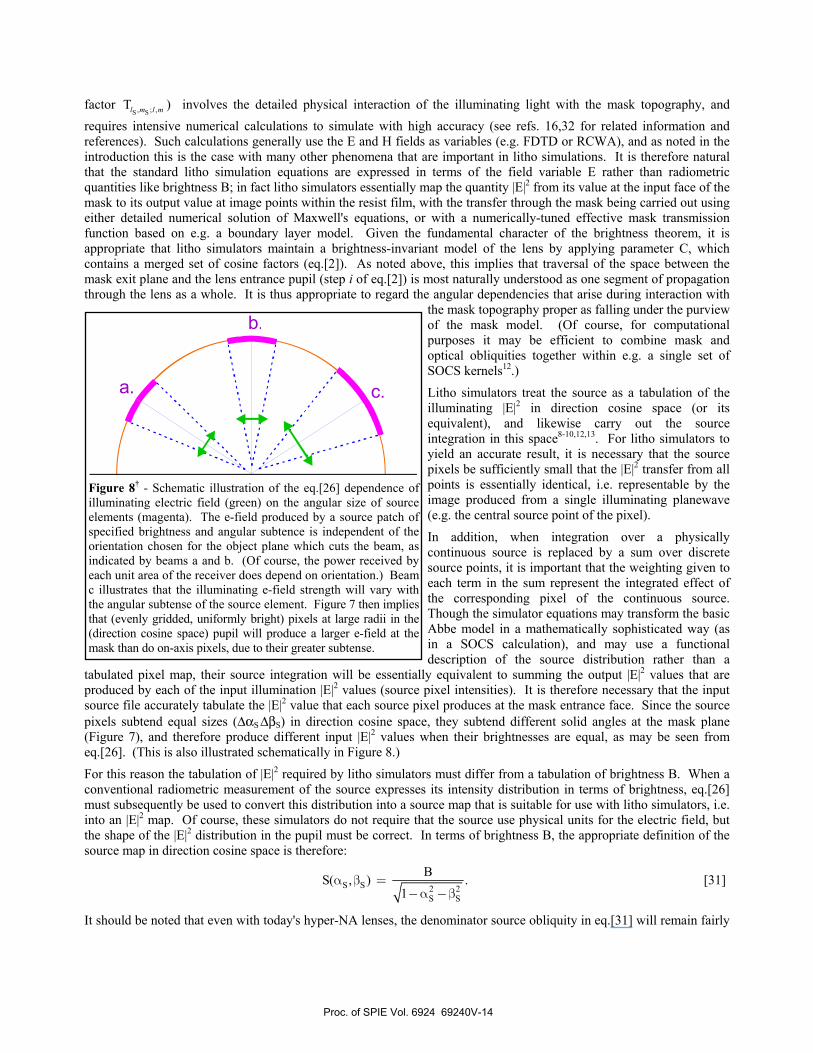
Figure 8† - Schematic illustration of the eq.[26] dependence of illuminating electric field (green) on the angular size of source elements (magenta). The e-field produced by a source patch of specified brightness and angular subtence is independent of the orientation chosen for the object plane which cuts the beam, as indicated by beams a and b. (Of course, the power received by each unit area of the receiver does depend on orientation.) Beam c illustrates that the illuminating e-field strength will vary with the angular subtense of the source element. Figure 7 then impliesthat (evenly gridded, uniformly bright) pixels at large radii in the (direction cosine space) pupil will produce a larger e-field at the mask than do on-axis pixels, due to their greater subtense.

factor S S, ; ,Tl m l m ) involves the detailed physical interaction of the illuminating light with the mask topography, and

requires intensive numerical calculations to simulate with high accuracy (see refs. 16,32 for related information and references). Such calculations generally use the E and H fields as variables (e.g. FDTD or RCWA), and as noted in the introduction this is the case with many other phenomena that are important in litho simulations. It is therefore natural that the standard litho simulation equations are expressed in terms of the field variable E rather than radiometric quantities like brightness B; in fact litho simulators essentially map the quantity |E|2 from its value at the input face of the mask to its output value at image points within the resist film, with the transfer through the mask being carried out using either detailed numerical solution of Maxwell's equations, or with a numerically-tuned effective mask transmission function based on e.g. a boundary layer model. Given the fundamental character of the brightness theorem, it is appropriate that litho simulators maintain a brightness-invariant model of the lens by applying parameter C, which contains a merged set of cosine factors (eq.[2]). As noted above, this implies that traversal of the space between the mask exit plane and the lens entrance pupil (step i of eq.[2]) is most naturally understood as one segment of propagation through the lens as a whole. It is thus appropriate to regard the angular dependencies that arise during interaction with

the mask topography proper as falling under the purview of the mask model. (Of course, for computational purposes it may be efficient to combine mask and optical obliquities together within e.g. a single set of SOCS kernels12.) Litho simulators treat the source as a tabulation of the illuminating |E|2 in direction cosine space (or its equivalent), and likewise carry out the source integration in this space8-10,12,13. For litho simulators to yield an accurate result, it is necessary that the source pixels be sufficiently small that the |E|2 transfer from all points is essentially identical, i.e. representable by the image produced from a single illuminating planewave (e.g. the central source point of the pixel). In addition, when integration over a physically continuous source is replaced by a sum over discrete source points, it is important that the weighting given to each term in the sum represent the integrated effect of the corresponding pixel of the continuous source. Though the simulator equations may transform the basic Abbe model in a mathematically sophisticated way (as in a SOCS calculation), and may use a functional description of the source distribution rather than a

tabulated pixel map, their source integration will be essentially equivalent to summing the output |E|2 values that are produced by each of the input illumination |E|2 values (source pixel intensities). It is therefore necessary that the input source file accurately tabulate the |E|2 value that each source pixel produces at the mask entrance face. Since the source pixels subtend equal sizes (∆αS ∆βS) in direction cosine space, they subtend different solid angles at the mask plane (Figure 7), and therefore produce different input |E|2 values when their brightnesses are equal, as may be seen from eq.[26]. (This is also illustrated schematically in Figure 8.) For this reason the tabulation of |E|2 required by litho simulators must differ from a tabulation of brightness B. When a conventional radiometric measurement of the source expresses its intensity distribution in terms of brightness, eq.[26] must subsequently be used to convert this distribution into a source map that is suitable for use with litho simulators, i.e. into an |E|2 map. Of course, these simulators do not require that the source use physical units for the electric field, but the shape of the |E|2 distribution in the pupil must be correct. In terms of brightness B, the appropriate definition of the source map in direction cosine space is therefore:

S S 2 2S S

BS( , ) .1

α β =−α −β

[31]

It should be noted that even with today's hyper-NA lenses, the denominator source obliquity in eq.[31] will remain fairly

Proc. of SPIE Vol. 6924 69240V-14

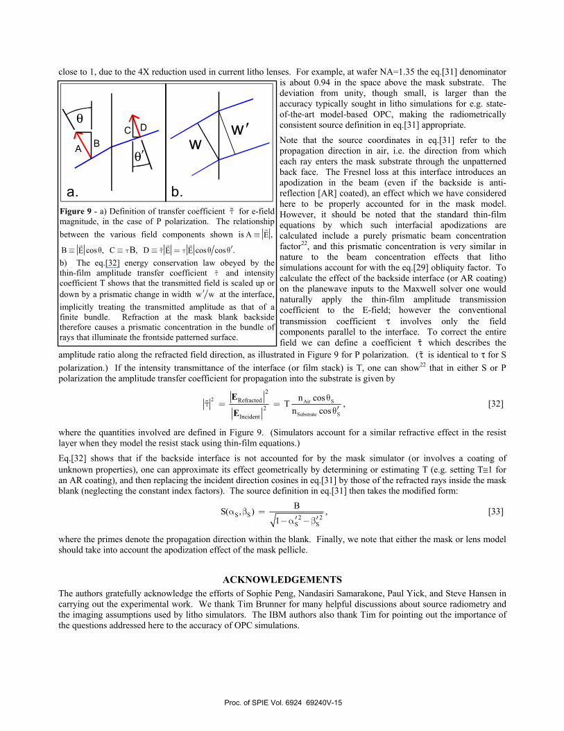
close to 1, due to the 4X reduction used in current litho lenses. For example, at wafer NA=1.35 the eq.[31] denominator is about 0.94 in the space above the mask substrate. The deviation from unity, though small, is larger than the accuracy typically sought in litho simulations for e.g. state-of-the-art model-based OPC, making the radiometrically consistent source definition in eq.[31] appropriate. Note that the source coordinates in eq.[31] refer to the propagation direction in air, i.e. the direction from which each ray enters the mask substrate through the unpatterned back face. The Fresnel loss at this interface introduces an apodization in the beam (even if the backside is anti-reflection [AR] coated), an effect which we have considered here to be properly accounted for in the mask model. However, it should be noted that the standard thin-film equations by which such interfacial apodizations are calculated include a purely prismatic beam concentration factor22, and this prismatic concentration is very similar in nature to the beam concentration effects that litho simulations account for with the eq.[29] obliquity factor. To calculate the effect of the backside interface (or AR coating) on the planewave inputs to the Maxwell solver one would naturally apply the thin-film amplitude transmission coefficient to the E-field; however the conventional transmission coefficient τ involves only the field components parallel to the interface. To correct the entire field we can define a coefficient τ which describes the

amplitude ratio along the refracted field direction, as illustrated in Figure 9 for P polarization. (τ is identical to τ for S polarization.) If the intensity transmittance of the interface (or film stack) is T, one can show22 that in either S or P polarization the amplitude transfer coefficient for propagation into the substrate is given by

2 Air S

Substrate S

2Refracted

2Incident

n cosT ,n cos

E

E

θτ = =

′θ [32]

where the quantities involved are defined in Figure 9. (Simulators account for a similar refractive effect in the resist layer when they model the resist stack using thin-film equations.) Eq.[32] shows that if the backside interface is not accounted for by the mask simulator (or involves a coating of unknown properties), one can approximate its effect geometrically by determining or estimating T (e.g. setting T≅1 for an AR coating), and then replacing the incident direction cosines in eq.[31] by those of the refracted rays inside the mask blank (neglecting the constant index factors). The source definition in eq.[31] then takes the modified form:

S S 2 2S S

BS( , ) ,1

α β =′ ′−α −β

[33]

where the primes denote the propagation direction within the blank. Finally, we note that either the mask or lens model should take into account the apodization effect of the mask pellicle.

ACKNOWLEDGEMENTS The authors gratefully acknowledge the efforts of Sophie Peng, Nandasiri Samarakone, Paul Yick, and Steve Hansen in carrying out the experimental work. We thank Tim Brunner for many helpful discussions about source radiometry and the imaging assumptions used by litho simulators. The IBM authors also thank Tim for pointing out the importance of the questions addressed here to the accuracy of OPC simulations.

a. b.

w'w

θ

θ'A BDC

Figure 9 - a) Definition of transfer coefficient τ for e-field magnitude, in the case of P polarization. The relationship between the various field components shown is A ,E≡

B cos ,E≡ θ C ,Bτ≡ D cos cos .E Eτ τ ′≡ = θ θ b) The eq.[32] energy conservation law obeyed by the thin-film amplitude transfer coefficient τ and intensity coefficient T shows that the transmitted field is scaled up or down by a prismatic change in width w w′ at the interface, implicitly treating the transmitted amplitude as that of a finite bundle. Refraction at the mask blank backside therefore causes a prismatic concentration in the bundle of rays that illuminate the frontside patterned surface.

Proc. of SPIE Vol. 6924 69240V-15

APPENDIX This Appendix shows that in calculations where the mask transmission is accurately known (either from rigorous E&M simulation, or by means of a numerically calibrated approximate model such as boundary layers or edge-DDM), the angular spectrum representation of a rigorous vector diffraction integral (the Franz formula) yields the same result as the standard angular spectrum propagation equation, as long as the mask exit plane is placed beyond all currents in the mask topography (i.e. offset slightly beyond the topography into free space, with optional back-propagation for re-focus). More generally, we can show that under these conditions all of the standard diffraction integrals (Helmholtz-Kirchoff, Stratton-Chu, Kottler, Franz) simplify considerably; in particular, they can be made to take the form of a "redundant" pair of integrals along the lines of an integration by parts for which the total differential is zero, causing each alternative in the by-parts integration to give an equal result. (An example of this has already been shown in the main text; if the equal results in eqs.[16] and [21] are added, the result resembles the integral of a chain-rule differentiation of the product of E and the Fourier propagator, and this product can be assumed on physical grounds to vanish at large radii within the mask exit plane, as is also suggested by the equality of the two equations.) When we apply the analysis below to any of these standard diffraction integrals, we find that each of a pair of terms can be derived (or analyzed) using a similar set of steps involving the angular spectrum representation. The physical basis for this simplification is the absence of source currents in the half-space beyond the mask exit pupil, the assumption that no back-propagated waves illuminate the mask patterns from the exit side, and in particular the fact that precise boundary conditions are automatically provided by modern mask simulation methods. We will exhibit the derivation in some detail for one of the terms in the Franz diffraction formula, as an illustration of how the full Franz result can be derived from an angular spectrum analysis. We will also sketch out the derivation for the complementary approach in which the Franz formula reduces to the eq.[8] angular spectrum propagator in free space. Both approaches depend on well-known results from spatial domain Fourier transformation of Maxwell's harmonic equations in free space, which we briefly review here. In free-space the E-field satisfies the homogeneous Helmholtz equation 2 2

0( k ) ( ) 0.∇ + =E r Substituting in the (purely mathematical) 2D inverse transform of eq.[6], we have

( ) ( ) ( ) ( )2

2 2 2 22 0

Mj , z10 d e , z k , z ,z2

⎧ ⎫⎡ ⎤⎪ ⎪∂⎪ ⎪⎪ ⎪⎢ ⎥= − + + + γ⎨ ⎬⎢ ⎥∂⎪ ⎪π ⎢ ⎥⎪ ⎪⎣ ⎦⎪ ⎪⎩ ⎭∫ k r k

k k k k kE

E E⋅ [34]

x ywhere d denotes dk dk .k Since this must hold for all values of z, we conclude that

( ) ( )2

2 22 0

, zk , z ,z

∂= − γ

∂k

kE

E [35]

from which we obtain in standard fashion the angular spectrum result in eq.[8] (and thence eq.[10]), for the case in which all waves are forward traveling. We will also make use of the angular spectrum results obtained by substituting the eq.[6] inverse transform into the free-space harmonic Maxwell equations 0jk 0∇× + =H E and 0∇⋅ = ∇⋅ =H E , namely

( ) ( ) ( ) ( )0k , z , z and , z , z 0 .= × ⋅ = ⋅ =k k k k k k kE H H E [36]

In Gaussian units, the Franz formula states that the field measured at a point rp is given by:25

( ) ( ) ( ) ( ) ( )P M P M M M P M MP P P

0

1 ˆ ˆd G , z d G , z ,jk

E r r r r H r r r r E r⎛ ⎞⎡ ⎤⎟ ⎡ ⎤⎜= ∇ × ∇ × × + ∇ × ×⎟⎜ ⎢ ⎥ ⎢ ⎥⎟⎟⎜ ⎣ ⎦ ⎣ ⎦⎝ ⎠∫ ∫ [37]

where the P subscript on ∇ indicates differentiation with respect to the measurement-point coordinates, and where the free-space Green's function G is given by

( )P M

0P M

2P M0

P Mjk j ( )e j eG , d .8 k4

− ⋅ −−= =

π γπ − ∫r r k r r

r r kr r

[38]

The right-hand form is the Weyl expansion, which, as suggested by eqs.[11] and [13], can be intuitively understood to

Proc. of SPIE Vol. 6924 69240V-16

represent the Green's function spherical wave as a superposition of plane waves that (by symmetry) are uniformly distributed in direction solid angle. We now show that the eq.[37] Franz formula for free-space propagation can be derived from the angular spectrum result of eq.[10] for free space propagation. (Later we will briefly sketch the reverse derivation.) Using vector identities and eq.[36], eq.[10] can be written

( ) ( ) ( )( )P P

P MP0P MP P

P0P P M MP P P P P

0 P

jk (z z )jk (z z )j j1 1 e ˆ, z d e e , z d e , z ,

2 2 k

γ −γ − ⎡ ⎤= = − × ×⎢ ⎥⎣ ⎦π π γ∫ ∫k r k rE r k k k k z kE E⋅ ⋅

[39]

where we have also employed eq.[15]. Using P PP M MP P

P P0 0jk (z z ) jk zj je e e eγ − − γ=k r k r⋅ ⋅ and the expression for the curl of a planewave, we have

( ) ( )( )P

MPP0

P P MP P P

0 P

jk zjj e e ˆ, z d , z .2 k

− γ

= − ∇ × ×π γ∫

k rE r k z kE

⋅ [40]

Substituting in the inverse transform of eq.[6]

( ) ( )( )P

P

MPP0MP P M M M

P P20 P

jk zjjj e e ˆ, z d d e , z .

4 k

− γ−= ∇ × ×

π γ∫ ∫k r

k rE r k r z E r⋅

⋅ [41]

According to the eq.[38] Weyl expansion, this can be written

( ) ( ) ( )( )P P M P M M MP ˆ, z 2 d G , , z .= ∇ × ×∫E r r r r z E r [42]

This is twice the right hand term of the Franz formula. Through similar steps we can likewise show that the left term also gives ( )P P, z 2.E r When the doubled right-hand term of the Franz formula is used as a standalone expression, the resulting diffraction integral (i.e. eq.[42]) is known as the Smythe formula18. It is also straightforward to show that when the Franz formula in free space is re-cast in terms of the angular spectrum, it simply expresses the eq.[8] propagation law. In brief, this can be shown by first using the above derivation of eqs.[35] and [36] from Maxwell's equations to derive the eq.[10] three-dimensional angular spectrum transform, and then using eq.[10] to replace the fields in the eq.[37] Franz formula by superpositions of plane waves (doing likewise with the Green's function via eq.[38]), and finally inverse transforming both sides of the resulting equation (by applying the

eq.[6] 2D Fourier transform). If one then repeatedly invokes the delta-function representation 2 j4 ( ) d eπ δ = ∫ k rr k ⋅ to simplify the nested integrals, one finds that the Franz formula reduces to a simple expression of the propagation law for the angular spectrum amplitudes (eq.[8]). These results show that the modern ability of rigorous Maxwell solvers or high accuracy thin-mask extensions to provide the field in the exit plane of the mask greatly simplifies the diffraction calculation for propagation to the far field. Under these conditions the basic angular spectrum approach used by litho simulators provides the same information as the most advanced classical diffraction integrals.

REFERENCES [1] T.C. Barrett, “Impact of illumination pupil-fill spatial variation on simulated imaging performance,” SPIE v.4000 - Optical Microlithography XIII (2000): p. 804. [2] C.T. Bodendorf, R.E. Schlief, and R. Ziebold, “Impact of measured pupil illumination fill distribution on lithography simulation and OPC models,” SPIE v.5377 - Optical Microlithography XVII: p. 1130. [3] A.E. Rosenbluth and N. Seong, “Global Optimization of the Illumination Distribution to Maximize Integrated Process Window,” SPIE v.6154 Optical Microlithography XIX (2006): p. 61540H. [4] D.G. Flagello, T. Milster, and A.E. Rosenbluth, “Theory of high-NA imaging in homogeneous thin films,” J. Opt. Soc. Am. A 13, no.1 (1996): p. 53.

Proc. of SPIE Vol. 6924 69240V-17

[5] H. Ries, “Thermodynamic limitations of the concentration of electromagnetic radiation,” J. Opt. Soc. Am. 72, no.3 (1982): p. 380. [6] D.G. Flagello and A.E. Rosenbluth, “Lithographic tolerances based on vector diffraction theory,” J. Vac. Sci. Technol. B 10, no.6 (1992): p. 2997. [7] M.S. Yeung, D. Lee, R.S. Lee, and A.R. Neureuther, “Extension of the Hopkins theory of partially coherent imaging to include thin-film interference effects,” SPIE v.1927 -- Optical/Laser Microlithography (1993): p. 452. [8] M. Born and E. Wolf, Principles of Optics, 5th ed. (Oxford: Pergamon, 1975). [9] J.W. Goodman, Statistical Optics (Wiley, 1985). [10] D.C. Cole, E. Barouch, U. Hollerbach, and S.A. Orszag, “Derivation and Simulation of Higher Numerical Aperture Scalar Aerial Images,” Jpn. J. Appl. Phys. 31 (1992): p. 4110 [11] N.B. Cobb and A. Zakhor, “A mathematical and CAD framework for proximity correction,” in SPIE v.2726 - Optical Microlithography IX, (1996), p. 208. [12] A.E. Rosenbluth, G. Gallatin, R.L. Gordon, W. Hinsberg, J. Hoffnagle, F. Houle, K. Lai, A. Lvov, M. Sanchez, and N. Seong, “Fast calculation of images for high numerical aperture lithography,” SPIE v.5377 Optical Microlithography XVII (2004): p. 615. [13] T.V. Pistor, “Electromagnetic Simulation and Modeling with Applications in Lithography” (University of California, Berkeley, 2001). [14] K. Lai, A.E. Rosenbluth, G. Han, J. Tirapu-Azpiroz, J. Meiring, A. Goehnermeier, B. Kneer, M. Totzeck, L.d. Winter, W.d. Boeij, and M.v.d. Kerkhof, “Modeling polarization for hyper-NA lithography tools and masks,” SPIE v.6520 - Optical Microlithography XX (2007): p. 65200D. [15] J. Tirapu-Azpiroz, A.E. Rosenbluth, K. Lai, C. Fonseca, and D. Yang, “Critical impact of mask electromagnetic effects on optical proximity corrections performance for 45nm and beyond,” Journal of Vacuum Science & Technology B 25, no.1 (2007). [16] A. Erdmann and P. Evanschitzky, “Rigorous electromagnetic field mask modeling and related lithographic effects in the low k1 and ultrahigh numerical aperture regime,” JM3 6, no.3 (2007): p. 031002. [17] B. Richards and E. Wolf, “Electromagnetic diffraction in optical systems II: Structure of the field in an aplanatic system,” Proc Roy Soc London Ser A 253 (1959): p. 358. [18] J.D. Jackson, Classical Electrodynamics, 2nd ed. (Wiley, 1975). [19] J.A. Stratton, Electromagnetic Theory (IEEE Press Series on Electromagnetic Wave Theory, 2007). [20] N. Kerwien, T. Schuster, S. Rafler, W. Osten, and M. Totzeck, “Vectorial thin-element approximation: a semirigorous determination of Kirchhoff's boundary conditions,” J. Opt. Soc. Am. A 24, no.4 (2007): p. 1074. [21] G. Gallatin, “High-numerical-aperture scalar imaging,” Applied Optics 40, no.28 (2001): p. 4958. [22] A.E. Rosenbluth, G. Gallatin, K. Lai, N. Seong, and R.N. Singh, “Topics in polarization ray tracing for image projectors,” SPIE - Volume 5875, Novel Optical Systems Design and Optimization VIII (2005): p. 587503. [23] P.C. Clemmow, The Plane Wave Spectrum Representation of Electromagnetic Fields (Oxford University Press, 1996). [24] J.W. Goodman, Introduction to Fourier Optics (McGraw-Hill, 1968). [25] C.T. Tai, “Direct Integration of Field Equations,” Progress in Electromagnetic Research 28 (2000): p. 339. [26] J. Tirapu-Azpiroz, “Analysis and Modeling of Photomask Near-Fields in Sub-Wavelength Deep Ultraviolet Lithography” (PhD, UCLA, 2004). [27] D.S. Jones, “Removal of an inconsistency in the theory of diffraction,” Proceedings of the Cambridge Philosophical Society 48 (1952): p. 733. [28] M.A. Alonso and R. Borghi, “Complete far-field asymptotic series for free fields,” Optics Letters 31, no.20 (2006): p. 3028 [29] J. Tirapu-Azpiroz and E. Yablonovitch, “Modeling of Near-Field effects in Sub-Wavelength Deep Ultraviolet Lithography,” in Future Trends of Microelectronics - 2003, ed. S. Luryi, J. Xu, and A. Zaslavsky (Wiley-IEEE Press), p. 80. [30] K. Adam, “Modeling of Electromagnetic Effects from Mask Topography at Full-Chip Scale,” SPIE v.5754 - Optical Microlithography XVIII (2004): p. 498. [31] A.T. Friberg, G.S. Agarwal, J.T. Foley, and E. Wolf, “Statistical wave-theoretical derivation of the free-space transport equation of radiometry,” J. Opt. Soc. Am. B 9, no.8 (1992): p. 1386. [32] J. Tirapu-Azpiroz, G.W. Burr, A.E. Rosenbluth, and M.S. Hibbs, “Massively-Parallel FDTD Simulations to Address Mask Electromagnetic Effects in Hyper-NA Immersion Lithography,” in Optical Microlithography XXI (San Jose: 2008).

Proc. of SPIE Vol. 6924 69240V-18