Production and Costs1. We move from behaviour of consumers to

behavior of producers2. Firms use economic resources to produce

goods & services and incur costs3. Firms make monetary payments to

resource owners to call them as explicit costs (ex. wages to workers)

4. These payments/costs together with implicit costs (opportunity costs of own resources) make up the firms costs of production

1

Theory of Production and Costs

We will look at:

1.Economic Costs and profits

2. Short-run Production Costs and Relationships

3. Long-run Production Costs and Relationships

2

Firm - a production unit• Every economy consists of thousands of firms that produce the goods and services that we enjoy everyday.

• Some firms are large-– they employ thousands of workers– Have large numbers of shareholders who share in the firm’s profits

• Other firms are small– They employ a few number of people – Owned by one man/ one family (sole proprietorship) or few people (partnership)

3

What Are Costs• According to the Law of SupplyLaw of Supply:

– Firms are willing to produce and sell a greater quantity of a good when the price of the good is higher.

– This results in a supply curve that slopes upward

• The Firm’s objective/goal:The economic objective / goal of the firm is to maximize profits

4

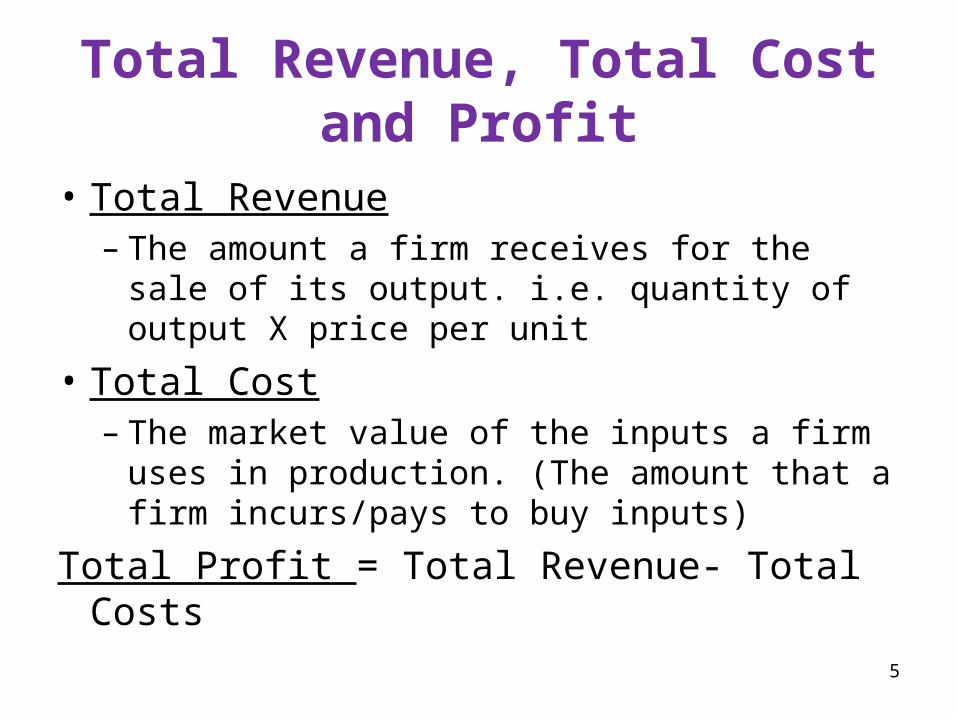
Total Revenue, Total Cost and Profit

• Total Revenue– The amount a firm receives for the sale of its output. i.e. quantity of output X price per unit

• Total Cost– The market value of the inputs a firm uses in production. (The amount that a firm incurs/pays to buy inputs)

Total Profit = Total Revenue- Total Costs

5

Total Revenue, Total Cost and Profit

Profit is the firm’s total revenue minus its total cost.

Profit = Total revenue - Total cost•Total Revenue is easy to compute: – it is the quantity of output the firm produces times the price at which it sells its output.

•Total Cost is more difficult to measure

6

Costs as Opportunity cost

• Recall that the cost of something is the value of what you give up/sacrifice to get it.

• Opportunity cost of an item refers to all those that must be foregone to acquire the item

• When the economist talks of a firm’s cost of production, they include all the opportunity costs of making its output of goods and services

7

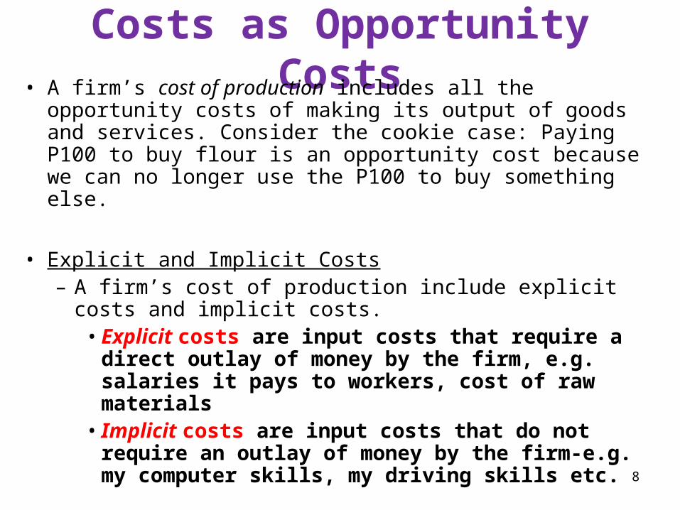
Costs as Opportunity Costs• A firm’s cost of production includes all the

opportunity costs of making its output of goods and services. Consider the cookie case: Paying P100 to buy flour is an opportunity cost because we can no longer use the P100 to buy something else.

• Explicit and Implicit Costs– A firm’s cost of production include explicit costs and implicit costs.•Explicit costs are input costs that require a direct outlay of money by the firm, e.g. salaries it pays to workers, cost of raw materials

• Implicit costs are input costs that do not require an outlay of money by the firm-e.g. my computer skills, my driving skills etc. 8

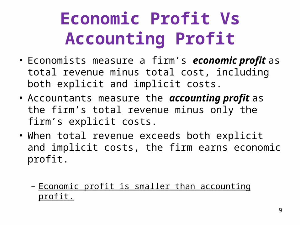
Economic Profit Vs Accounting Profit

• Economists measure a firm’s economic profit as total revenue minus total cost, including both explicit and implicit costs.

• Accountants measure the accounting profit as the firm’s total revenue minus only the firm’s explicit costs.

• When total revenue exceeds both explicit and implicit costs, the firm earns economic profit.

– Economic profit is smaller than accounting profit.

9

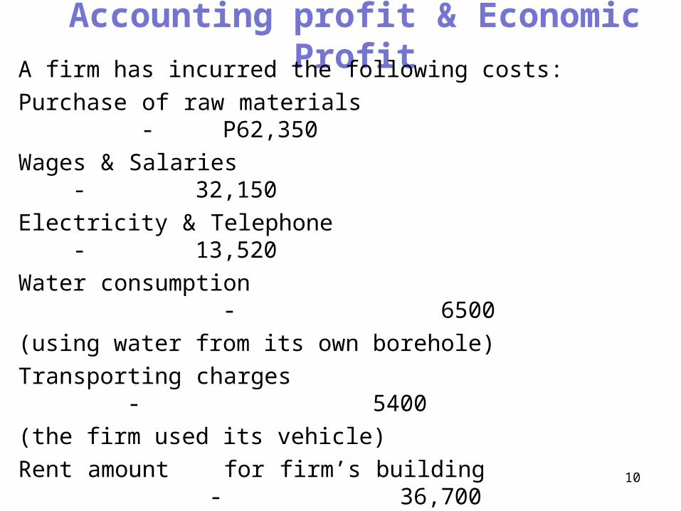
Accounting profit & Economic ProfitA firm has incurred the following costs:

Purchase of raw materials - P62,350Wages & Salaries - 32,150Electricity & Telephone - 13,520Water consumption - 6500(using water from its own borehole) Transporting charges - 5400(the firm used its vehicle)Rent amount for firm’s building - 36,700(The firm used its own factory building)The value of the firm’s owner’s managerial abilities - 52,000(No manager is employed)Total Revenue of the firm - 275,750Calculate Accounting profit and economic profit

10

Production• The total amount of output The total amount of output produced by a firm is a function produced by a firm is a function of the levels of input usage by of the levels of input usage by the firm.the firm.

• The Production Function– The production function shows the relationship between quantity of inputs used to make a commodity and the quantity of output of that commodity/good produced.

11

Short-run & Long-run production relationships

• Short run is a period too brief for a firm to alter its plant capacity. The firm can for a time increase its output by adding only units of variable resources like labour to its fixed plant capacity.

• Long run is the period of time long enough to enable producers to change the quantities of all the resources they employ and increase production..

12

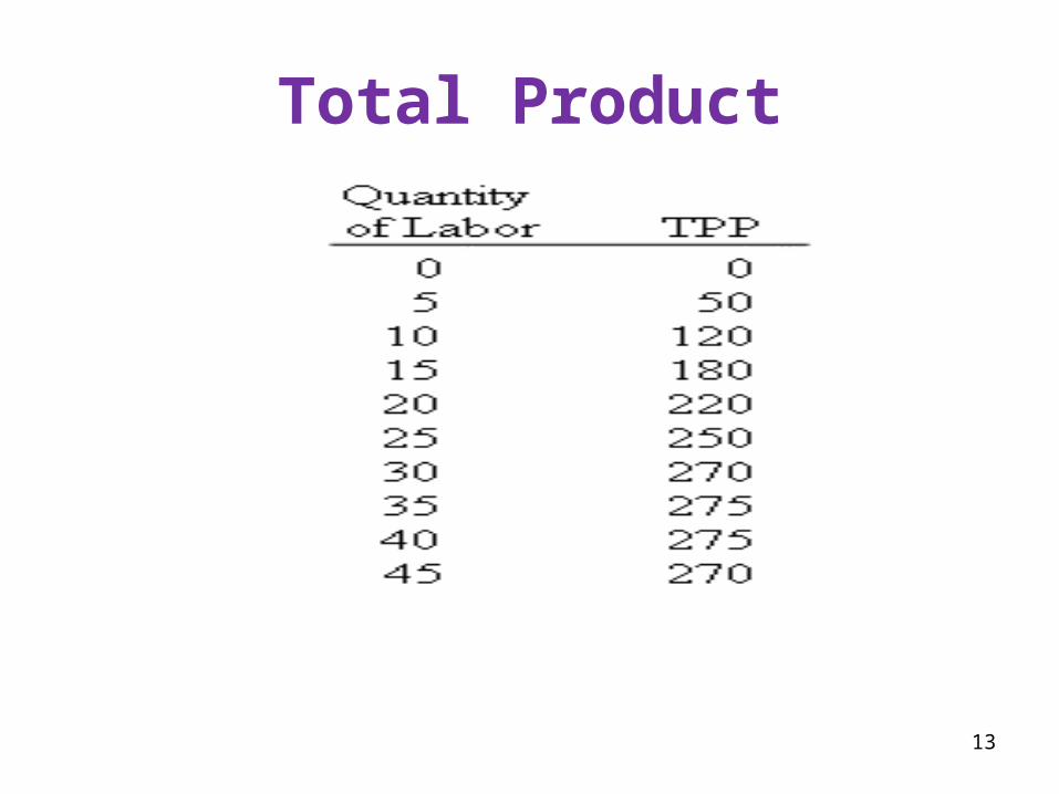
Total Product

13

14

Total Product (TP), Average Product (AP) & Marginal product (MP)

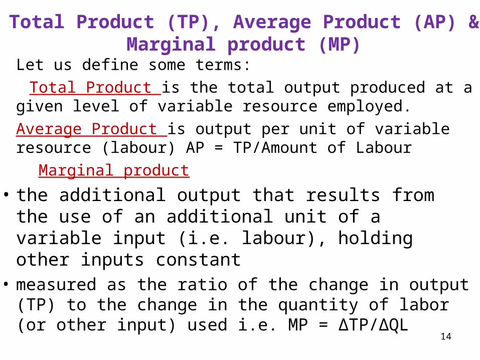
Let us define some terms: Total Product is the total output produced at a given level of variable resource employed.Average Product is output per unit of variable resource (labour) AP = TP/Amount of Labour

Marginal product• the additional output that results from the use of an additional unit of a variable input (i.e. labour), holding other inputs constant

• measured as the ratio of the change in output (TP) to the change in the quantity of labor (or other input) used i.e. MP = ∆TP/∆QL

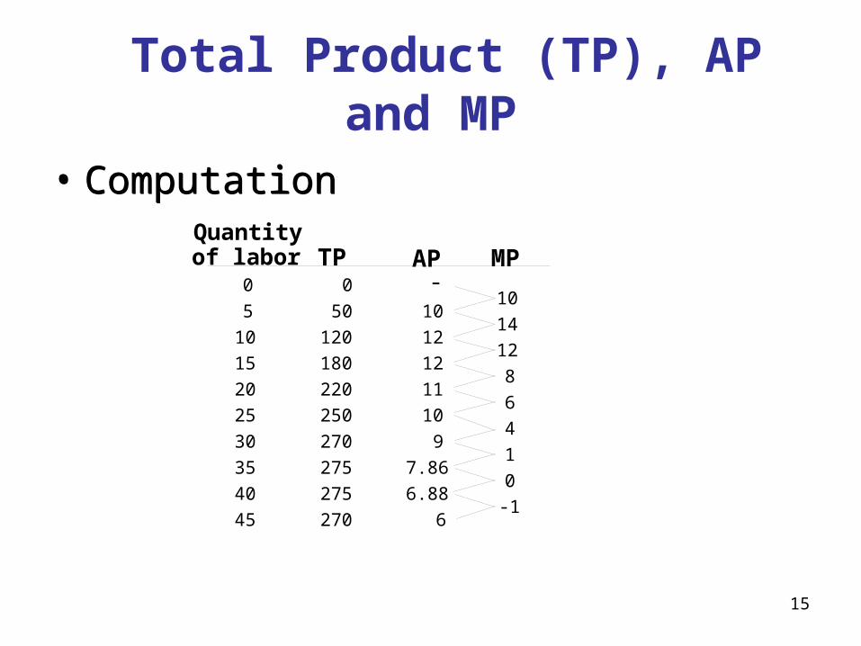
Total Product (TP), AP and MP

• Computation

15

Quantityof labor TP AP

051015202530354045

MP0

50120180220250270275275270

-10121211109

7.866.88

6

10141286410-1

• Computation

Law of Diminishing Returns or Law of Diminishing Marginal Product

• In the short run, diminishing returns operate. As the level of a variable input rises in a production process in which other inputs are fixed, output increases at decreasing rate and then declines after reaching certain maximum level.

• The Law of Diminishing Returns states that as successive units of a variable resource (say labour) are added to a fixed resource (say capital or land), beyond some point, marginal product that can be attributed to each additional unit of the variable resource will decline.

•Example: As more and more workers are hired at a firm, each additional worker contributes (MP) less and less to production because the firm has a limited amount of fixed equipment. 16

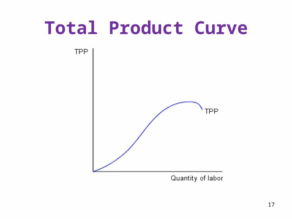
Total Product Curve

17

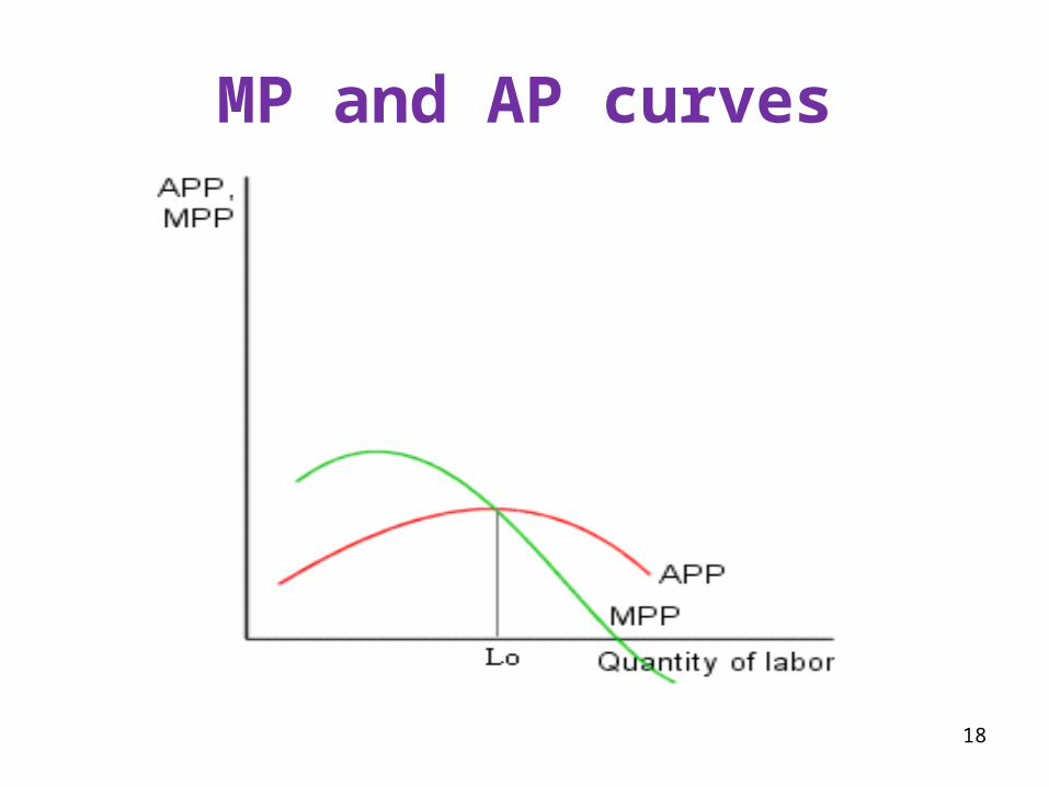
MP and AP curves

18

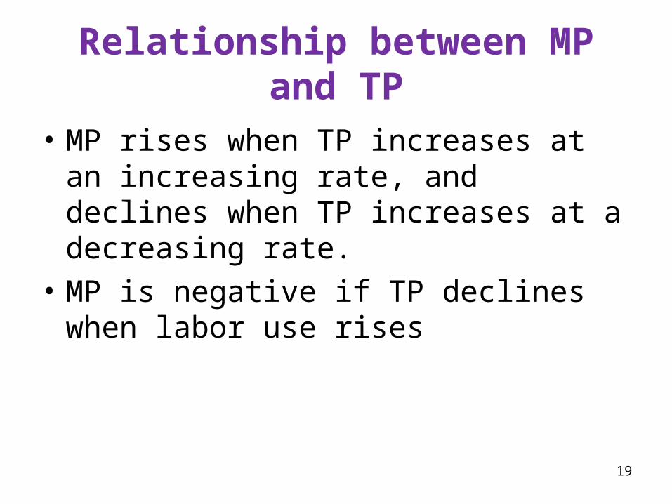
Relationship between MP and TP

• MP rises when TP increases at an increasing rate, and declines when TP increases at a decreasing rate.

• MP is negative if TP declines when labor use rises

19

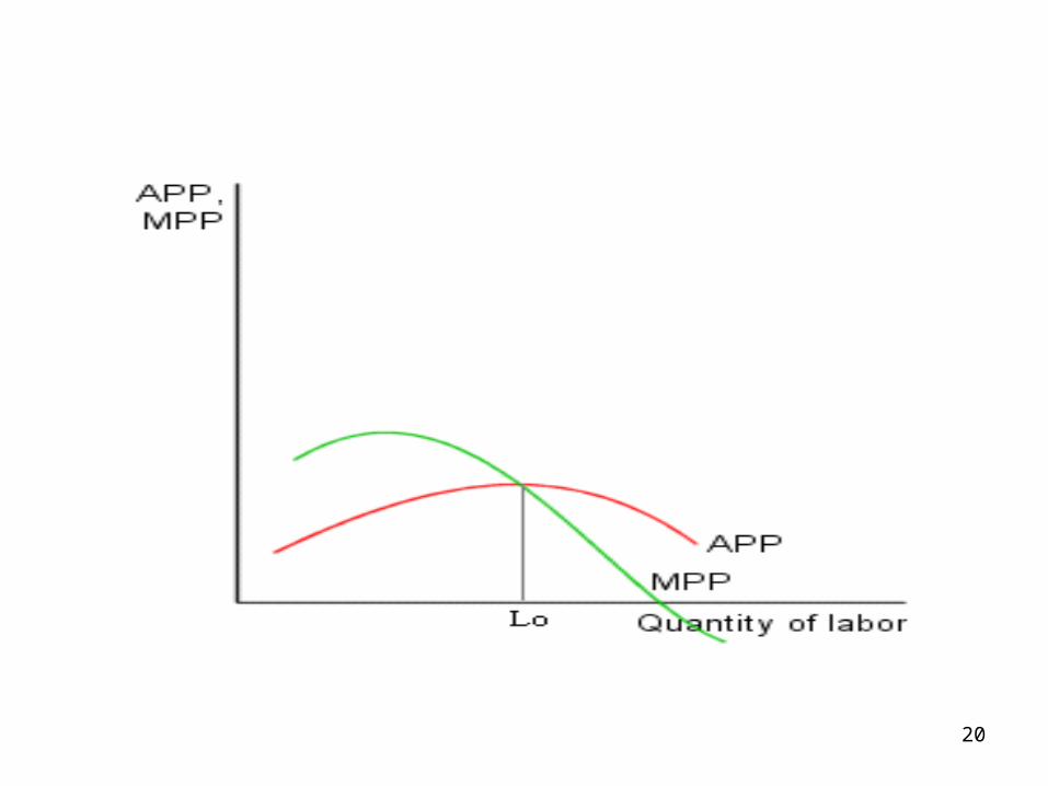
Relationship of AP and MP

20

Relationship between AP and MP

•AP rises when MP > AP•AP falls when MP < AP•AP is at a maximum when MP = AP

21

From Production to Costs• The relationship between the quantity a firm can produce and its costs determines pricing decisions.

• The total-cost curve shows this relationship graphically

22

Short Run Costs• Short run costs have two components:

– Fixed costs – costs that do not vary with the level of output. Fixed costs remain constant/ same at all levels of output (even when output equals zero) in the short run.

– Variable costs – costs that vary with the level of output (Variable costs are zero when output is zero). Variable costs arise when production of goods is done.

23

Short run Costs con..• Total Costs in the short run:

– Total Fixed Costs (TFC)– Total Variable Costs (TVC)– Total Costs (TC) – TC = TFC + TVC

24

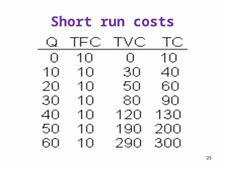
Short run costs

25

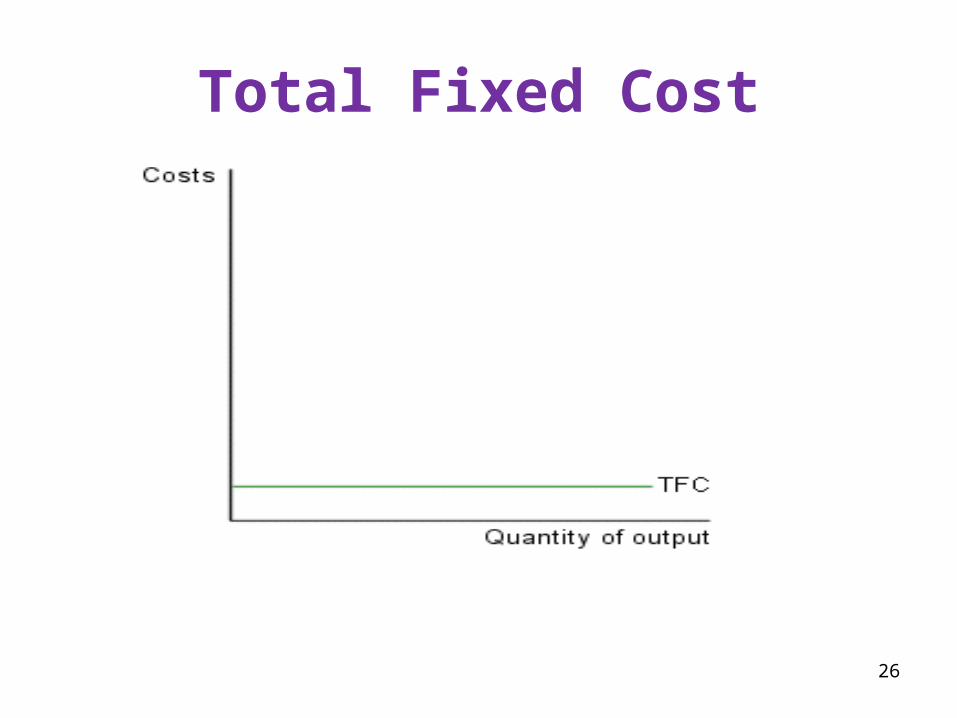
Total Fixed Cost

26

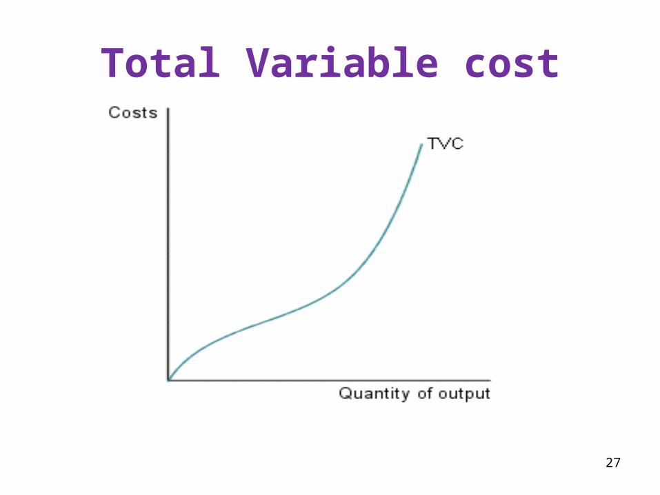
Total Variable cost

27

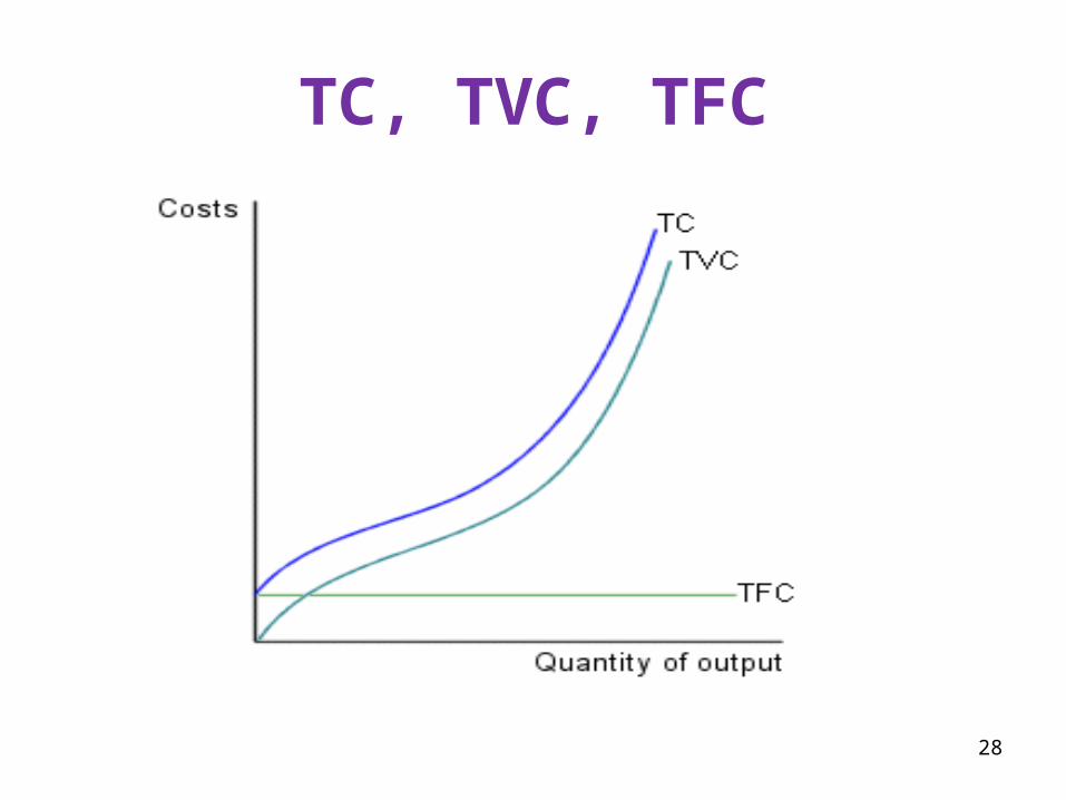
TC, TVC, TFC

28

Average costs• Average Costs• - Average Total cost (ATC)

– Average Fixed Costs (AFC)– Average Variable Costs (AVC)– Average Total Costs (ATC)– ATC = AFC + AVC

29

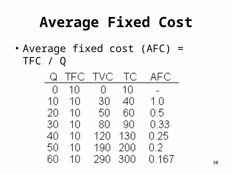
Average Fixed Cost• Average fixed cost (AFC) = TFC / Q

30

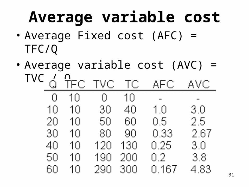
Average variable cost• Average Fixed cost (AFC) = TFC/Q

• Average variable cost (AVC) = TVC / Q

31

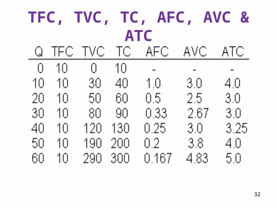
TFC, TVC, TC, AFC, AVC & ATC

32

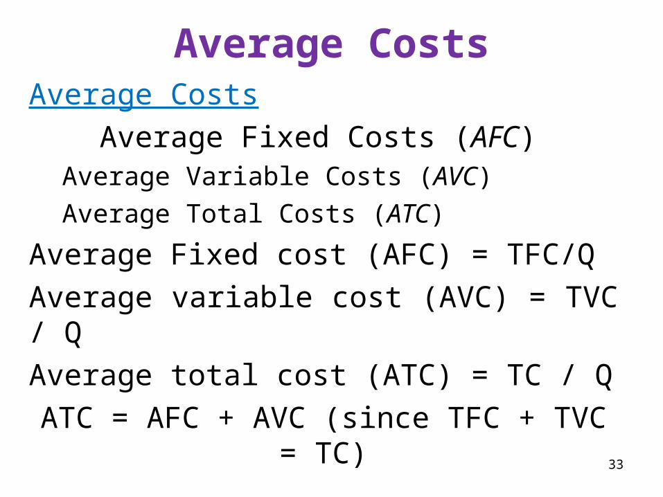
Average CostsAverage Costs Average Fixed Costs (AFC)

Average Variable Costs (AVC)Average Total Costs (ATC)

Average Fixed cost (AFC) = TFC/QAverage variable cost (AVC) = TVC / QAverage total cost (ATC) = TC / QATC = AFC + AVC (since TFC + TVC

= TC) 33

Marginal cost• .

– Marginal cost helps answer the following question:•How much does it cost to produce an additional unit of output?

34

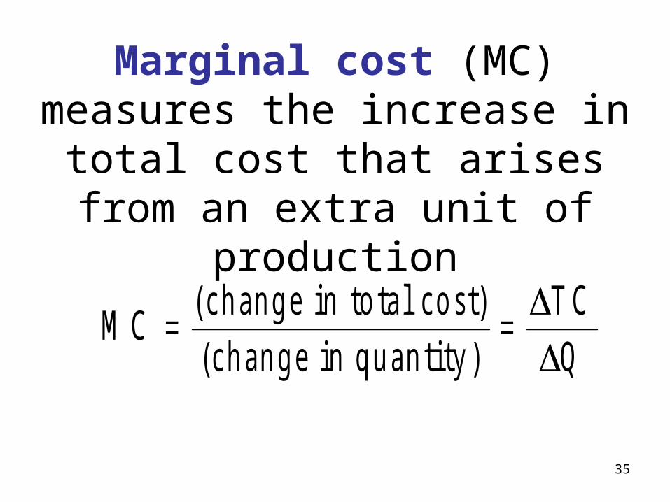
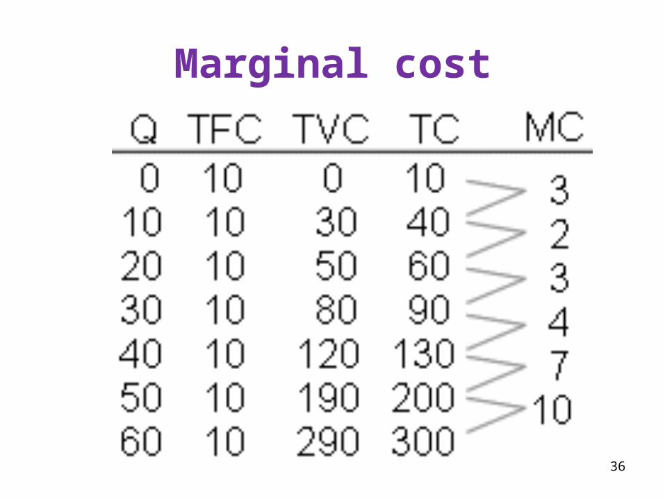
Marginal cost (MC) measures the increase in total cost that arises from an extra unit of

productionM C T C

Q (change in total cost)(change in quantity)

35

Marginal cost

36

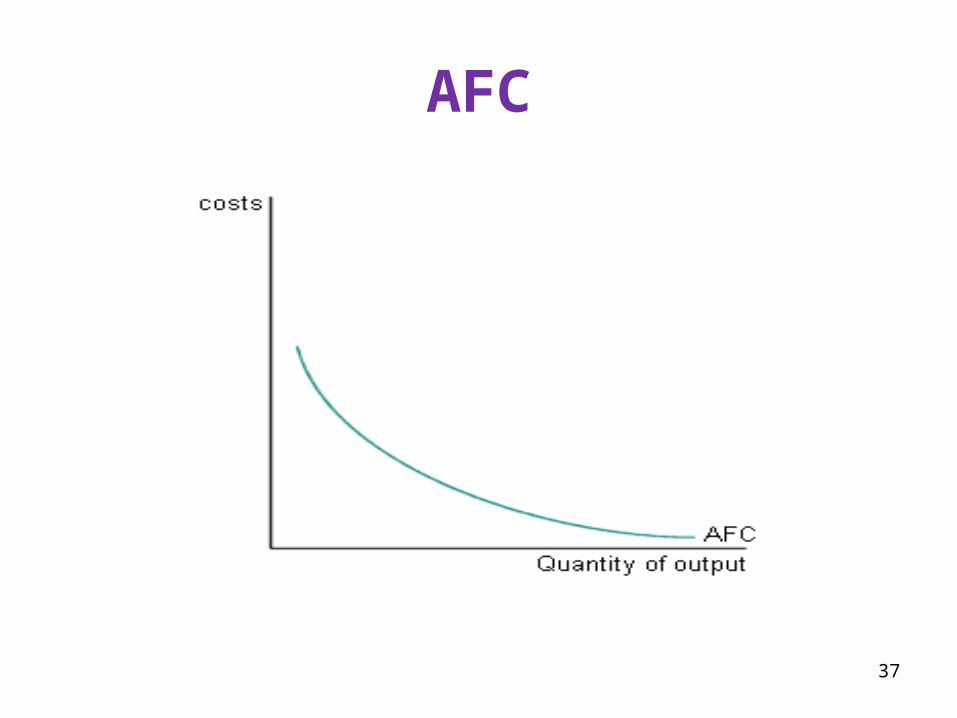
AFC

37

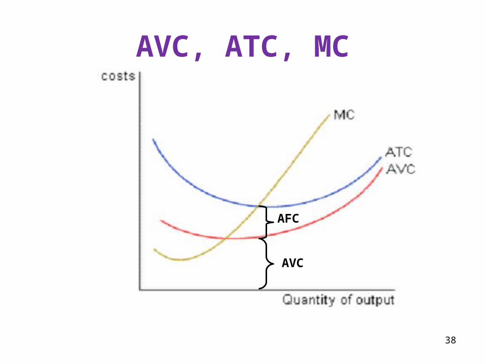
AVC, ATC, MC

AVC

AFC

38

ATC • ATC=AFC + AVC• AFC always declines as output rises because fixed cost is spread over larger number of units

• AVC rises as output rises because of Diminishing Marginal Product

• ATC reflects the shape of the AFC and AVC curves

39

MC, AVC & ATC• MC rises with the quantity of output• The AC curve is U-shaped • The MC curve intersects the AVC and ATC at their respective minimum points

• MC curve reflects the law of DMP– At low levels of output, few workers are hired, much of the equipment (fixed resources) are unused

– MP of an extra worker is large– MC of an extra unit produced is small– At larger outputs, MP is of an extra worker is low, MC of an extra unit produced is large

40

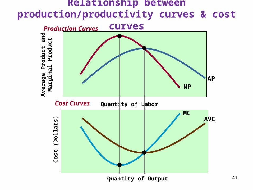
Relationship between production/productivity curves & cost

curvesAv

erage

Produc

t and

Marg

inal

Pro

duct

Quantity of Labor

MPAP

MCAVC

Quantity of Output

Cost

(Do

llars)

Cost Curves

Production Curves

41

Relationship between production/productivity curves & cost curves in the short run

• Assuming labour is the only variable resource/input & its price is constant:

– When MP is rising, MC is falling– When MP is maximum, MC is minimum – When MP is falling, MC is rising,– When MP is rising, AVC is falling and– When AP is maximum, AVC is minimum – When AP is falling, AVC is rising

42

LONG RUN costs & curves• Long run costs: For many firms, in the long run there is no such division of total costs as fixed and variable costs because all costs will change. In the long run, fixed costs become variable costs.

• A firm’s long-run cost curves differ from its short-run costs.

43

L-R cost curves

44

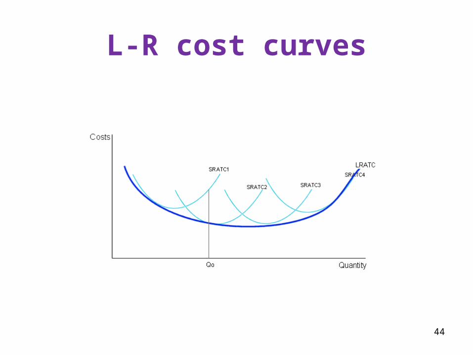
LR cost and LRATC curve• In the long run, a firm may choose its level of capital, and will select a size of firm that provides the lowest level of ATC.

• Each point on the ATC gives the minimum average cost of producing the corresponding level of output as the firm’s scale of operations (size) increases. I.e. The firm grows in terms of its size of investment and the use of resources in the long run.

• Firm does not face diminishing returns in the long run because the size of all resources increases and there is no such fixed costs and variable costs as all costs will change.

• Firm will derive economies of scale and diseconomies of scale in the long run.

45

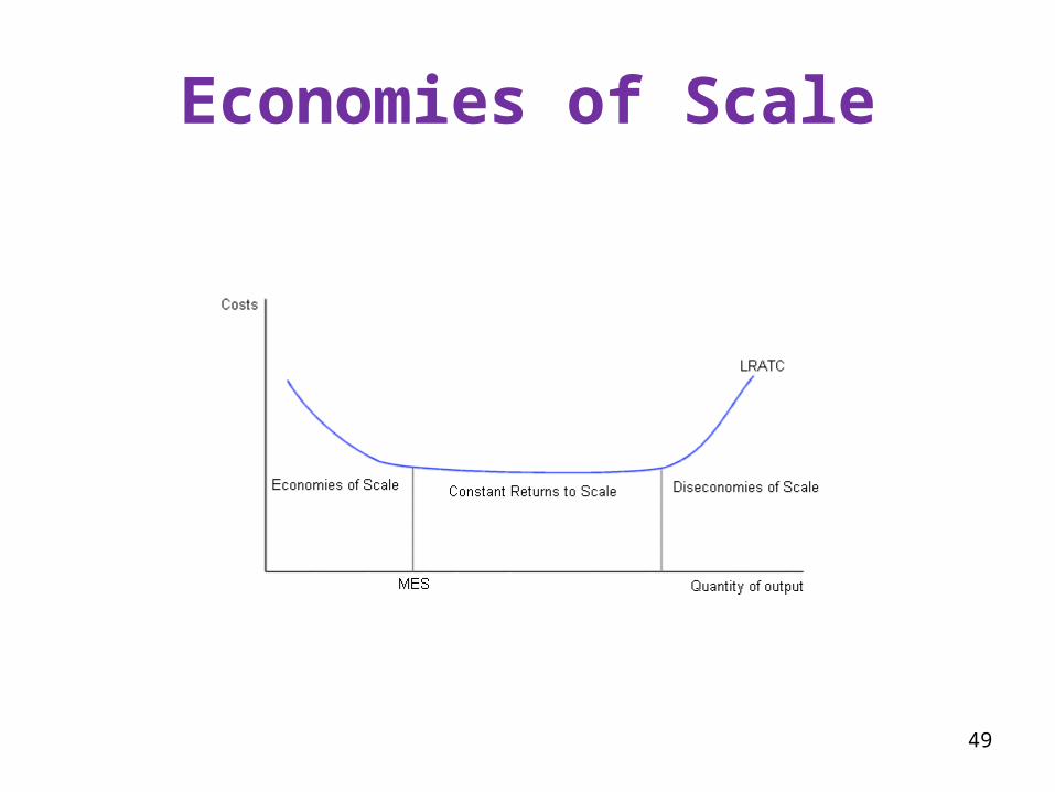
Economies and Diseconomies of Scale• Economies of scale refer to the property whereby long-

run average total cost falls as the quantity of output increases.– Economies of scale are the factors that contribute to lower average total cost (ATC) with the increase in output, as the size of the firm rises in the long run

– Sources/Factors: specialization and division of labor, indivisibilities of capital, etc.1.Division of labor–available at large scale production and helps save time that would be lost by moving from one role to another2.Specialisation, Managerial specialization – Better use of specialists by undertaking greater specialization in management3.Capital efficiency – small firms often cannot afford the most efficient equipment. Bigger the size of the firm, higher the economies of scale4.Learning by doing – available at large scale production46

Economies and Diseconomies of Scale con..• Diseconomies of scale refer to the property

whereby long-run average total cost rises as the quantity of output increases when the firm’s size grows beyond particular size.Diseconomies of scale – factors that influence to raise average total cost as the size of the firm rises in the long run

Sources/Factors: – increased cost of managing and coordination as firm size rises – e.g., executive far from the production line

– Lack of adequate control over production and resources

– Managerial bureaucracy – Workers may feel far removed from their employers & may care less about working efficiently. 47

Economies and Diseconomies of Scale con…• Given the following info indicate if the

industry exhibits, Economies of scale or diseconomies of scale– A 1% increase in all resources used in production cause output to increase by more than 1% is Increasing returns to scale/economies of scale

– A 1% increase in all resources used in production causes output to increase by less than 1% is decreasing returns to scale/diseconomies of scale

- A 1% increase in all resources used in production

causes output to increase by 1% is Constant returns to scale 48

Economies of Scale

49

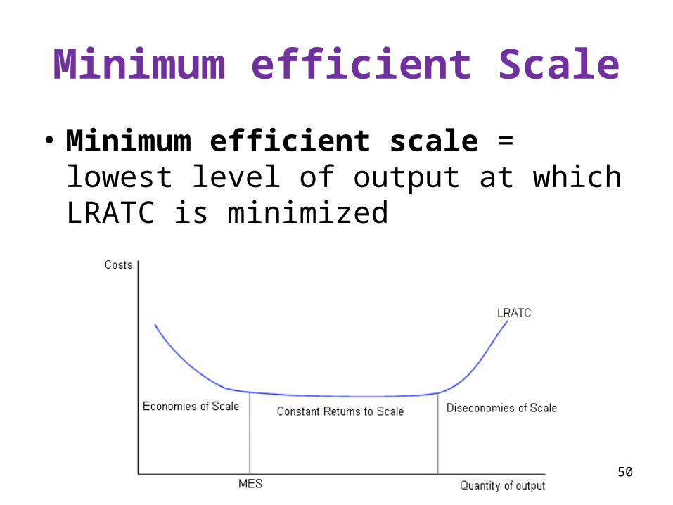
Minimum efficient Scale• Minimum efficient scale = lowest level of output at which LRATC is minimized

50

MES & industry structure• Economies & diseconomies are important determinants of industry structure

• An industry where economies of scale are: - few & diseconomies set in quickly, i.e. MES occurs at low output levels will be populated by small firms (size is not an advantage)– large and diseconomies set in only at very

high levels of output, i.e., MES occurs at high levels of output will be populated by few large firms

– Continue over an extended range of output, i.e., MES at low output and extend to high output levels, will be populated by firms of different sizes. Size doesn’t matter in competitiveness 51

Summary• The goal of firms is to maximize profit, which equals total revenue minus total cost.

• When analyzing a firm’s behavior, it is important to include all the opportunity costs of production.

• Some opportunity costs are explicit while other opportunity costs are implicit.

52

Summary• A firm’s costs reflect its production process.

• A typical firm’s production function gets flatter as the quantity of input increases, displaying the property of diminishing marginal product.

• A firm’s total costs are divided between fixed and variable costs. Fixed costs do not change when the firm alters the quantity of output produced; variable costs do change as the firm alters quantity of output produced.

53

Summary• Average total cost is total cost divided by the quantity of output.

• Marginal cost is the amount by which total cost would rise if output were increased by one unit.

• Average cost and marginal cost first fall as output increases and then rise.

54

Summary• The average-total-cost curve is U-shaped.

• The marginal-cost curve always crosses the average-total-cost curve at the minimum of ATC.

• A firm’s costs often depend on the time horizon being considered.

• In particular, many costs are fixed in the short run but variable in the long run.

55