Embed Size (px)
Citation preview

Science of Computer Programming 35 (1999) 191–221www.elsevier.nl/locate/scico
Tractable constraints in �nite semilattices
Jakob Rehof a;∗;1, Torben �. MogensenbaMicrosoft Research, One microsoft Way, Redmond, WA 98052, USA
bDIKU, Department of Computer Science, Universitetsparken 1, DK-2100 Copenhagen I, Denmark
Abstract
We introduce the notion of de�nite inequality constraints involving monotone functions in a�nite meet-semilattice, generalizing the logical notion of Horn-clauses, and we give a linear timealgorithm for deciding satis�ability. We characterize the expressiveness of the framework of def-inite constraints and show that the algorithm uniformly solves exactly the set of all meet-closedrelational constraint problems, running with small linear time constant factors for any �xed prob-lem. We give an alternative technique for reducing inequalities to satis�ability of Horn-clauses(HORNSAT) and study its e�ciency. Finally, we show that the algorithm is complete for a max-imal class of tractable constraints, by proving that any strict extension will lead to NP-hardproblems in any meet-semilattice. c© 1999 Elsevier Science B.V. All rights reserved.
Keywords: Finite semilattices; Constraint satis�ability; Program analysis; Tractability;Algorithms
1. Introduction
It is well known that many program analysis problems can be solved by generatinga set of constraints over a �nite domain and then solving these. Examples include owanalysis (closure analysis) [24], binding time analysis [15, 4, 5, 11], usage count anal-ysis [23], multiplicity inference for region-size analysis [3], strictness analysis [16, 1].In many cases such analyses can be speci�ed by annotated-type systems [27], and theanalyses can be implemented using non-standard type-inference, where constraints be-tween type annotations are collected from the program. Some more detailed examplestaken from ow analysis and usage count analysis are given in Section 6.In this paper we show how to solve certain classes of constraints over �nite domains
e�ciently, and characterize classes that are not tractable. The solution methods can beused as a tool for analysis designers, and the characterization can help the designerrecognize when an analysis may have bad worst-case behaviour.
∗ Corresponding author. Fax: (+1) 425-705-2404.E-mail addresses: [email protected] (J. Rehof), [email protected] (T.�. Mogensen)1 This work was done while the �rst author was at DIKU.
0167-6423/99/$ - see front matter c© 1999 Elsevier Science B.V. All rights reserved.PII: S 0167 -6423(99)00011 -8
192 J. Rehof, T.�. Mogensen / Science of Computer Programming 35 (1999) 191–221
Our classi�cation of constraint problems evolves from the notion of de�nite in-equalities, which can be seen as a generalization of the logical notion of Horn clauses[14, 10], from the two-point boolean lattice of the truth values to arbitrary �nite semi-lattices. De�nite inequality constraints are inequalities of the form �6A where � is anexpression built from an arbitrary set of function symbols denoting monotone func-tions and A is either a variable or a constant. We show that the �xpoint computationtechnique of Kildall [22] and the decision procedure for Horn-clause satis�ability ofDowling and Gallier [10] can be adapted to the framework of general �nite semilat-tices, leading to an algorithm, called D, for solving sets of de�nite constraints, withthe following properties:– The algorithm runs in linear time with small constant factors, for any �xed �nitesemilattice.
– The algorithm operates uniformly over all �nite semilattices and all monotone func-tions, and hence it can be thought of as a general solver for the uniform problemwhich is parameterized on both the domain (semilattice), the monotone functionsand the constraint set. The algorithm can therefore serve as a general purpose, o�-the-shelf solver, which supports a whole range of program analyses.
We are interested in understanding the range of applicability of the frameworkof de�nite constraints, i.e., we would like to know, what problems can algorithmD solve e�ciently? At a super�cial level, the applicability of the algorithm is re-stricted to the class of de�nite constraints, since the algorithm assumes its constraintset parameter to be of this form. However, constraint problems which are not givenin de�nite form might be transformed into equivalent de�nite ones, and hence thequestion above translates into the problem of determining the expressive power ofde�nite inequality constraints: which problems can be expressed by equivalent setsof de�nite constraints? In order to demonstrate that generality does not come at thecost of sacri�cing e�ciency, our investigation of this latter question is accompa-nied by an analysis of the cost of the transformations into de�nite form. We showthat– Algorithm D solves exactly the set of all meet-closed relational constraint problems,modulo linear time transformations, with small constant factors, into de�nite form.Hence, the generic use of the algorithm is feasible, remaining within the e�cientlinear time framework.
Here, the notion of a relational constraint problem is a generalization of the logicalnotion introduced by Schaefer [26] to prove his remarkable Dichotomy Theorem, ac-cording to which any relational boolean constraint problem either falls into one of foureasily recognizable tractable (polynomial time solvable) classes, or else the problemis NP-complete. One of the four tractable classes corresponds exactly to Horn-clauses.For recent generalizations of Schaefer’s Dichotomy Theorem in various directions, see[12, 7, 21].By composing Birkho�’s Representation Theorem for �nite lattices with Schaefer’s
Dichotomy Theorem we get an easy proof of the following completeness property foralgorithm D:

J. Rehof, T.�. Mogensen / Science of Computer Programming 35 (1999) 191–221 193
– Any strict extension of the class of meet-closed problems solved by algorithm Dwill lead to an NP-complete uniform problem.
– For distributive lattices we can exhibit simple meet-closed problems with a �xedsemilattice and a �xed set of relations such that no matter how the problems areextended with non-meet-closed relations the resulting problems will be NP-complete.
This shows that algorithm D is complete for a maximal tractable class of problems,namely the meet-closed ones, and the theorems on non-extendability can be used torecognize the borderline between tractable and intractable problems.Finally, we show that de�nite constraint problems can be represented by boolean
Horn-implications, leading to an alternative linear time solution procedure, by reductionto the procedure of Dowling and Gallier [10]. We compare algorithm D to reductionto Horn-clauses with respect to time and space e�ciency.The paper is organized as follows. Section 2 introduces the framework of constraint
problems involving monotone functions on �nite semilattices, and Section 3 de�nes therestricted form of de�nite inequalities and introduces algorithm D, which appears inAppendix A. Section 4 introduces the generalized framework of relational problems; theexpressiveness of de�nite constraints is studied (Section 4.1) and the alternative methodof transformation into logical Horn-clauses is described (Section 4.2). The results onintractability of extensions of the meet-closed framework are given in Section 5.Section 6 contains some more detailed examples of how the results presented inthis paper can be used to reason about concrete program analysis problems. Finally,Section 7 compares the behaviour of an implementation of algorithm D and an imple-mentation of constraint solving by reduction to Horn-clauses. Section 8 concludes thepaper.
2. Monotone function problems
Let P be a poset and F a �nite set of monotone functions f :Paf →P with af¿1the arity of f. We call the pair �=(P; F) a monotone function problem (MFP).Given �=(P; F) we let T� denote the set of �-terms, ranged over by �; � and givenby � ::= � | c |f(�1; : : : ; �af) where c ranges over constants in P; �; �; range overa denumerably in�nite set V of variables and f is a function symbol corresponding tof∈F . Constants and variables are collectively referred to as atoms, and we let A rangeover atoms. We assume a �xed enumeration of V;V= v1; v2; : : : ; vn; : : : For each num-ber m¿0 we let Vm denote the sequence of the m �rst variables in the enumeration ofV. Let �∈ Sm for some set S. We write [�]i for the ith coordinate of �; i∈{1; : : : ; m}.Any �∈ Sm is implicitly considered a mapping � :Vm → S by de�ning �(vi) to be [�]i,for i∈{1; : : : ; m}. For �∈ Sm; 16k6m we let �↓k =([�]1; : : : ; [�]k)∈ Sk .A constraint set C over � is a �nite set of formal inequalitites of the form �6�′
with �; �′ ∈T�. The set of distinct variables occurring in a term � is denoted Var(�),and if C is a constraint set, then Var(C) denotes the set of distinct variables

194 J. Rehof, T.�. Mogensen / Science of Computer Programming 35 (1999) 191–221
occurring in C. In this paper, we always assume that Var(C)=Vm for some m.If �∈Pm, � a (P; F)-term with Var(�)⊆Vm, then � is called a valuation of � inP. A valuation is tacitly lifted to an interpretation <�=� of �, given by <�=�= �(�),<c=�= c; <f(�1; : : : ; �k)=�=f(<�1=�; : : : ; <�k =�). Let Var(�)⊆Vm. Then the m-ary func-tion denoted by � is the map <�= :Pm →P given by <�=(�)= <�=�. Since every functionin F is assumed to be monotone, the function <�= is easily seen to be monotone, forevery (P; F)-term �.Let �; �′ be (P; F)-terms. If Var(�)∪Var(�′)⊆Vm, �∈Pm, we say that � satis�es
the constraint �6�′, written P; � |= �6�′, i� <�=�6<�′=� is true in P. If C is a con-straint set over (P; F), Var(C)⊆Vm, �∈Pm, we say that � is a valuation of C inP; we say that � satis�es C, written P; � |= C, i� P; � |= �6�′ for every constraint�6�′ in C. We say that C is satis�able if and only if there exists a valuation � ofC in P such that P; � |= C. The set of solutions to C, denoted Sol(C), is the set{�∈Pm |P; � |= C;m= |Var(C)|} (|Var(C)| denotes the size of Var(C)).If �=(P; F) is an MFP, then we de�ne the decision problem �-SAT to be the fol-
lowing: Given a constraint set C over �; determine whether C is satis�able over P.We assume that f∈F are given by af-dimensional operation matrixes Mf withMf[x1; : : : ; xaf ] =f(x1; : : : ; xaf). Under this representation, evaluating a function f atgiven arguments x1; : : : ; xaf is a constant time operation, and hence evaluating an ar-bitrary functional term � is O(|�|) (we measure the size of a term by |�|, the numberof occurrences of symbols (constants, variables and function symbols) in �; the sizeof a constraint set C, denoted |C|, is the number of occurrences of symbols in C).If P is a lattice, the component P is assumed to be given as the set of elements ofP together with an additional operation matrix, Mt, de�ning the least upper bound ofL, i.e., Mt[x; y] = x t y. From this we can recover the order relation of P, using thatx6y i� xty=y. This representation will be referred to as the matrix representation.As we shall see, this is also an appropriate representation when P is a semilattice,since this case will be reduced to the case where P is a lattice.There are many problems � for which �-SAT is NP-hard (every problem �-SAT is
obviously in NP, since we can guess and verify a solution non-deterministically inpolynomial time). Simple examples of this occur whenever P is a �nite lattice andboth the least upper bound (t) and the greatest lower bound (u) operations are in theF-component of �:
Example 1. For any non-trivial �nite lattice L, the problem �=(L; {u;t}) is NP-complete, by reduction from CNF-SAT (propositional satis�ability, [13]): We can assumethat L contains at least one atom, i.e., an element c∈L such that c 6=⊥ and for everyx∈L; ⊥6x¡c implies x=⊥. Any logical clause C (a set of literals representing theirdisjunction) can be written in the form
(P1 ∧ · · · ∧Pk)⇒ (Q1 ∨ · · · ∨Qm)
where the Pi are the propositional variables which occur negated in the clause, and theQi are the variables which occur unnegated; here the empty disjunction is the logical

J. Rehof, T.�. Mogensen / Science of Computer Programming 35 (1999) 191–221 195
constant false, and the empty conjunction is true. Then C is logically satis�able if andonly if
(P1 u · · · u Pk)6(Q1 t · · · t Qm)
is satis�able under the additional constraints that �6c for every variable � in C, trueis interpreted as c and false as ⊥, where c is any �xed atom of L.
Also, the structure of the poset P is important for complexity, see [25].The foregoing observations show that we need to impose restrictions on problems
to make them tractable. In the following development, we shall generally assume thatP is a meet-semilattice. Note, though, that the whole development transfers to join-semilattices by lattice-theoretic dualization.
3. De�nite problems
Let �=(P; F) be an MFP. A constraint set C over � in which every inequality isof the form �6A, with an atom on the right hand side, is called de�nite. A de�niteset C = {�i6Ai}i∈I can be written C =Cvar ∪Ccnst where Cvar = {�j6�j}j∈J are thevariable expressions in C, having a variable (�j) on the right-hand side of 6, andCcnst = {�k6ck}k∈K are the constant expressions in C, having a constant (ck) on theright-hand side. Notice that propositional Horn-clauses are a special case of de�niteinequalities:
Example 2. Satis�ability of de�nite inequalities over �=(2; {u}), with 2 the two-point boolean lattice, is exactly the HORNSAT problem (satis�ability of propositionalHorn clauses [14, 10]) since Horn clauses have the form P1 ∧ · · · ∧Pn ⇒ Q, which isequivalent to the inequality P1 u · · · u Pn6Q.
A term � will be called simple if � is a constant, a variable or has the form�=f(A1; : : : ; Am); i.e., there are no nested function applications; a constraint set C iscalled simple if all terms in it are simple. The L-normalization →L transforms a de�-nite set into a simple and de�nite set: let C be de�nite, C =C′ ∪{f(: : : g(�) : : :)6A}with Var(C)=Vm and � a tuple of terms, and de�ne →L by
C→L C′ ∪{f(: : : vm+1 : : :)6A; g(�)6vm+1}Normalizing a set with respect to →L expands the set with only a small constantfactor:
Lemma 1. The reduction →L is strongly normalizing; and if C∗ is a normal form ofa de�nite set C; then C∗ is de�nite with |C∗|63|C|.
Proof. Given de�nite set C, let ‖C‖ denote the number of distinct occurrences offunction symbols that are nested under a function symbol in C; it is easy to see that if

196 J. Rehof, T.�. Mogensen / Science of Computer Programming 35 (1999) 191–221
C→L C′ then ‖C′‖= ‖C‖−1, and hence no L-reduction sequence starting from C canhave more than ‖C‖ steps. Also, if C→L C′, then |C′|= |C|+ 2. Moreover, we have‖C‖6|C|, since |C| counts the total number of occurrences of symbols in C, whereas‖C‖ counts only a subset. It follows that, if C∗ is a normal form of C, we must have
|C∗|62‖C‖+ |C|62|C|+ |C|=3|C|The normal form C∗ is obviously de�nite, since C is.
Monotonicity guarantees that solving an L-normalized set is equivalent to solvingthe original set:
Lemma 2. If C→L C′ then Sol(C)= {�′ ↓m | �′ ∈Sol(C′)} where Var(C)=Vm.
Proof. Let C =C′′ ∪{f(: : : g(�) : : :)6A}; Var(C)=Vm with
C→L C′′ ∪{f(: : : vm+1 : : :)6A; g(�)6vm+1}=C′
Suppose � is a solution to C. De�ne �′ by �′(vi)= �(vi) for i6m and �′(vm+1)=<g(�)=�. Then
f(: : : �′(vm+1) : : :)=f(: : : <g(�)=� : : :)6<A=�= <A=�′
(we used <A=�= <A=�′, since vm+1 does not occur in A) and so �′ solves the �rstinequality of the reduct. For the second, we have
<g(�)=�′= <g(�)=�= �(vm+1)
where we used vm+1 =∈Var(g(�)) at the �rst equation. So �′ solves the second inequalityalso. We have shown the left-to-right inclusion.Assume, for the other inclusion, that �′ ∈Sol(C′). De�ne �= �′ ↓m. Then (since �′
solves C′)
<g(�)=�′6�′(vm+1)
and therefore, by monotonicity, we have
f(: : : <g(�)=� : : :)=f(: : : <g(�)=�′ : : :)6f(: : : �′(vm+1) : : :)6<A=�′= <A=�
where we used again that vm+1 occurs neither in A nor in g(�). This shows that�= �′ ↓m is a solution to C.
Fig. 4 in Appendix A gives an algorithm, called D, for solving de�nite constraintsover an MFP �=(L; F) with L a �nite lattice. 2 Algorithm D exploits L-normalization
2 Algorithm D is similar to the technique of Kildall [22] for fast �xed point computation in data- owframeworks and also to the linear time algorithm of Dowling and Gallier [10] for solving the HORNSAT-problem. Compare also the functional dependency closure algorithm of Beeri and Bernstein [2]. In fact,the iteration step of algorithm D is easily seen to be equivalent to a search for the least �xed point of amonotone operator F on a lattice, since the least �xed point of F is identical to the least post-�xed pointof F . We already observed (beginning of Section 3) that de�nite inequalities strictly subsume Horn clauses.See Sections 4.1 and 4.2 for more on the connection to Horn clauses.
J. Rehof, T.�. Mogensen / Science of Computer Programming 35 (1999) 191–221 197
to achieve linear time worst case complexity. Later, we shall change D slightly intoan algorithm D> which works for meet-semilattices.Correctness of algorithm D follows from the properties:
(1) after every update of the current valuation � at �, �(�) increases strictly in theorder of L, so in particular, termination follows, since L has �nite height;
(2) the iteration step �nds the least solution � to the set of variable expressions in C,so if any solution to C exists, then � must also satisfy the constant expressions,by monotonicity of all functions <�=.
Since the correctness proof is a straightforward consequence of the properties mentionedabove, we leave out the proof of the following theorem.
Theorem 3 (Correctness). If C has a solution over �; then it has a minimal solution;and algorithm D outputs � the minimal solution of C; and if C has no solution; thenthe algorithm fails.
We analyse the complexity of algorithm D, showing that it runs in linear time witha small constant factor for �xed problem �. Let h(L) denote the height of a �nitelattice L, i.e., the maximal length of a chain in L.
Theorem 4 (Complexity). For �xed MFP � algorithm D runs in time O(|C|) andperforms at most 3h(L) · |C| basic computations on input C.
Proof. Initialization: We can assume (Lemma 1) that C is in L-normal form moduloan expansion by a factor 3 (hence |C| below is at worst three times the size of theinput set). It is easy to see that initialization can be done in time of the order O(|C|).We use that arrays are assumed to be indexed by variables, and every test of the form�; L |= �6� (or the negation of such) can be performed in constant time, by L-normalform. A detailed argument is straightforward and is left out.Iteration: We amortize the number of times the test of the conditional in the for-
loop, �; L 6|= �6 , can be executed in total on input C, in the worst case. We observethat each time an item Clist[�][k] is inspected in this test the current valuation � hasincreased strictly (w.r.t. the order on L) at �. It follows that no single item Clist[�][k]can be inspected more than h(L) times, since � cannot increase more than h(L) timesat �. Now, the number of entries in Clist[�] is equal to the number of occurrencesof variable � in C (cf. description of Clist, Appendix A). Since the number of itemsin total in Clist is therefore bounded by |C|, it follows that no more than h(L) · |C|single inspections can be performed over a complete run of the algorithm on input C.The bound on the number of tests implies that all the other instructions in the iterationstep can at most be executed h(L) · |C| times over a complete run of the algorithm, oninput C. By L-normal form, all instructions are constant time (depending only on thearity of function symbols in �, which is held �xed). Since the �nal test at the outputstep is clearly computable in time O(|C|), we have shown that, at any control pointof the algorithm, the instruction at that point can consume at most h(L) · |C| units oftime in total on input C.

198 J. Rehof, T.�. Mogensen / Science of Computer Programming 35 (1999) 191–221
Algorithm D operates uniformly in �, so it can be considered a decision procedurefor the uniform problem parametric in � and C. In this case, taking h(L)= |L| in theworst case, |L|amax the size of the function matrixes with amax the maximal arity offunctions in �, we have input size N = |L|+ |L|amax + |C|. With log-cost for a matrixlook-up we get a maximum cost of O(amax · log |L|) for a basic computation, resultingin O(amax · log |L| · |L| · N ) worst case behaviour for the uniform problem.Algorithm D generalizes to the cases where the poset is a �nite meet-semilattice, as
follows. Let P> denote the lattice obtained from P by adding a top element >, takingc6> for all c∈P. We change algorithm D by adding the test if ∃�:�(�)=> thenFAIL at the beginning of the output step. We extend the functions in � such thatf(x1; : : : ; xaf)=> if any xi=>. This modi�cation of algorithm D will be referred toas algorithm D>. Algorithm D> is obviously sound, by soundness of algorithm D, andit is a complete decision procedure for semilattices, since if P has no top element andthe least solution to the variable expressions in C maps a variable to the top elementof P>, then clearly C can have no solutions in P.
4. Relational problems
Inequality constraints are a special case of the much more general framework ofrelational constraints. A relational constraint problem is a pair �=(P;S) with P a�nite poset and S a �nite set of �nite relations R⊆PaR , with 16aR (the arity ofR). Any R⊆Pk is called a relation over P. A relational constraint set C over � isa �nite set of �-terms of the form R(A1; : : : ; AaR) where A ranges over variables inV and constants drawn from P. The size of a constraint term t=R(A1; : : : ; AaR) is|t|= aR; the size |C| of a constraint set is the sum of the sizes of all terms in C. Wesay that a constraint set C is satis�able if there exists a valuation � of C in P such that(<A1=�; : : : ; <AaR =�)∈R for every term R(A1; : : : ; AaR) in C. If Var(C)=Vm, then Sol(C)is the set of valuations �∈Pm satisfying C. We de�ne the decision problem �-SAT tobe: Given a constraint set C over �; is C satis�able? If x∈Pm and 16i6m then[x]i denotes the ith coordinate of x. We use the vector notation x=(x1; : : : ; xm), and ifR⊆Pm we write R(x) as an abbreviation for R(x1; : : : ; xm) also when this expressionis considered a term.
4.1. Representability
We are interested in the following question: How many relational constraint problemscan be (e�ciently) solved using algorithm D? This translates to the question: Howmany problems can be transformed into de�nite inequality problems and what is thecost of the transformation?A relation R⊆Pm is called representable with respect to a constraint problem
�=(P;S) if R=Sol(C) for some constraint set C over �. We say that a problem �is a problem with inequality if the order relation 6 on P is representable with respect

J. Rehof, T.�. Mogensen / Science of Computer Programming 35 (1999) 191–221 199
to �. We say that a problem � has minimal solutions if Sol(C) has a minimal elementwith respect to 6 for any constraint set C over � with Sol(C) 6= ∅. If �=(P;S) withP a meet-semilattice and it holds for all R∈S that x; y∈R implies xuy∈R, then �is said to be a meet-closed problem. A relational problem �=(P;S) is representablein de�nite form if P is a meet-semilattice and there exists an MFP � such that for allconstraint sets C over � there exists a de�nite set C′ over � with Sol(C)= Sol(C′).Suppose that R⊆Pm is a meet-closed relation, P a meet-semilattice. Then de�ne the
partial function HR :Pm →Pm by HR(x)=∧ ↑R (x) where ↑R (x)= {y∈Pm | y¿x;
R(y)} and with HR unde�ned if ↑R (x) = ∅. Then HR is monotone when de�ned, i.e.,∀xy∈dom(HR): x6y⇒HR(x)6HR(y), and if ↑R (x) 6= ∅, then x∈dom(HR). More-over, for all x∈dom(HR) one has HR(x)¿x, since every y∈↑R(x) satis�es y¿x, andso we have
∧ ↑R (x)¿x.
Lemma 5. x∈R if and only if x∈dom(HR) and HR(x)6x.
Proof. If x∈R then x∈↑R(x), hence ↑R (x) 6= ∅, x∈dom(HR), and HR(x)6x. On theother hand, if x∈dom(HR) and HR(x)6x, then one has HR(x)= x, and since R ismeet-closed we have R(HR(x)), hence R(x).
We can now characterize the class of relational problems which can be solved usingalgorithm D, i.e., the problems which can be expressed by de�nite inequalities.
Theorem 6 (Representability). (1) Let �=(P;S) with P a meet-semilattice. Then �is representable in de�nite form if and only if � is meet-closed. In particular; if � ismeet-closed; then any constraint set C over � can be represented by a de�nite andsimple constraint set C′ with |C′|6m(m+2) · |C| where m is the maximal arity of arelation in S.(2) Let �6=(P;S) be a relational constraint problem with inequality; P arbitrary
poset. Then the following conditions are equivalent:(i) �6 has minimal solutions.(ii) �6 is meet-closed and P is a meet-semilattice.(iii) �6 is representable in de�nite form.
Proof. (1): (⇒) If � is representable in de�nite form, then for R∈S, R⊆Pk one hasSol(CR)=R with CR= {R(�1; : : : ; �k)}. By assumption there is a de�nite set C overa problem � with Sol(C)=Sol(CR)=R. But for �∈T�<�= is monotone, hence forany �; �′ ∈Sol(C) and any de�nite inequality �6A in C one has <�=(� u �′)6<�=� u<�=�′6<A=�u<A=�′= <A=(�u�′), hence any de�nite set C has Sol(C) meet-closed, henceR must be meet-closed.(⇐) If � is meet-closed, then (Lemma 5) � is representable in de�nite form,
hence it can be solved using algorithm D or D>, as follows. For every R∈S aterm t=R(A1; : : : ; Am) is equivalent, by Lemma 5, to HR(A1; : : : ; Am)6(A1; : : : ; Am),which can be written in de�nite form as Ct = {Hi
R(A1; : : : ; Am)6Ai | i=1 : : : m}, with

200 J. Rehof, T.�. Mogensen / Science of Computer Programming 35 (1999) 191–221
HiR(x)= [HR(x)]i, all monotone (when de�ned), by Lemma 5. Note that |Ct |= aR(|t|+2)= aR(aR + 2). If P is not a lattice, we use algorithm D> starting with a set ofextended relations S>= {R∪>aR |R∈S} with >aR the top element in (P>)aR ; thenall functions Hi
R :Pm →P are total and monotone. Hence, solving a set C over a meet-
closed problem �=(P;S) is equivalent to solving the de�nite and simple constraintset C′=
⋃t ∈C Ct over �=(P; F) with F =
⋃R∈S{Hi
R | ∈ {1; : : : ; aR}}.(2). (i)⇒ (ii) Since �6 has inequality, we can assume w.l.o.g. that S contains the
order relation 6 on P. Then Sol({�6�})=P, hence (by minimality of solutions) Phas a bottom element, ⊥. For any x; y∈P, consider C =
⋃z∈↓({x;y}){z6�}, where
↓({x; y})= {z ∈P | z6x; z6y}. Since P has a bottom element, we have ↓ ({x; y}) 6= ∅,and since x; y∈Sol(C) it follows by minimality of solutions that Sol(C) has a leastelement, which is
∨ ↓({x; y})= xuy. This shows that P is a meet-semilattice. Tosee that � is meet-closed, let R∈S and x; y∈R, and consider Cx;y =(
⋃aRj=1{�j6[x
uy]j})∪{R(�1; : : : ; �aR)}. Since x; y∈Sol(Cx;y), Sol(Cx;y) has a least element, z. Thenz¿xuy by construction of Cx;y, but also z6xuy because x; y∈Sol(Cx;y). Moreover,z ∈R by construction of Cx;y, and hence xuy= z ∈R. We have shown (i)⇒ (ii). Theimplication (ii)⇒ (iii) follows from item (1) of the present theorem, and (iii)⇒ (i) istrue, since by Theorem 3 any de�nite problem with solutions has minimal solutions.
Observe that property 1 of Theorem 6 can be seen as a strict generalization ofthe well-known fact that a set R⊆ 2k of boolean vectors is de�nable by a set ofpropositional Horn-clauses if and only if R is closed under conjunction. 3 Under thisview, the notion of de�nite inequalities generalizes the notion of Hornpropositions fromthe boolean case of 2 to an arbitrary meet-semilattice. 4
We have seen that any meet-closed problem can be represented by de�nite, func-tional constraints. Conversely, consider distributive constraint sets over an MFP, i.e.,constraint sets C where all �6�′ ∈C have the right-hand side �′ built from distributivefunctions only. 5 Distributive sets strictly include the de�nite ones, but every distribu-tive set can be represented by a relational set over a meet-closed problem, since thefunctions in F can be regarded as relations (graphs), hence (Theorem 6(1)) algorithmD can solve any �-SAT problem restricted to distributive constraint sets. In practice,it may be convenient to translate a distributive set directly into a de�nite one, usingthe auxiliary functions Hg, de�ned thus: let g :Pm →P with P a meet-semilattice; then
3 The de�nability condition for propositional Horn-clauses is a special case of a much more general modeltheoretic characterization of Horn-de�nability in �rst-order predicate logic, by which an arbitrary �rst-ordersentence � is logically equivalent to a Horn-sentence if and only if � preserves reduced products of models;see [6] or [17] for in-depth treatments of this result. See also [9].4 Note that in de�nite inequalities we are allowed to use any monotone functions, whereas in the special
case of Horn-implications we may use only one function, the meet operation. It is easy to see that onecannot, in general, de�ne an arbitrary meet-closed relation using only the meet operation of the semilattice,since, for instance, any set C of inequalities in one variable using only the meet function must be convex(i.e., x; y∈Sol(C) and x6z6y imply z∈Sol(C).) So, for instance, taking L to be the three element chain0¡1¡∞, the subset {∞; 0} is meet-closed but not convex and hence it cannot be de�ned using just themeet operation.5 A function f is distributive if f(xu y)=f(x)uf(y).

J. Rehof, T.�. Mogensen / Science of Computer Programming 35 (1999) 191–221 201
Hg :P→Pm is the partial function given by Hg(x)=∧{y∈Pm | x6g(y)} with Hg
unde�ned if no y∈Pm satis�es y6g(x). If P is a lattice, then Hg is a total function,and it is always monotone. We have
Lemma 7. Let f :Pn →P; g :Pm →P with g distributive. Then f(x)6g(y) if andonly if f(x)∈dom(Hg) and Hg(f(x))6y.
Proof. Assume f(x)6g(y). Then y∈{z |f(x)6g(z)}, hence f(x)∈dom(Hg) withHg(f(x))6y. Assume f(x)∈dom(Hg) with Hg(f(x))6y. Then (g◦Hg)(f(x))6g(y),since g is (distributive and therefore) monotone. For any w∈dom(Hg) one has, bydistributivity of g, that (g◦Hg)(w)=
∧{g(z) |w6g(z)}¿w. Hence we have f(x)6(g◦Hg)(f(x))6g(y).
The transformation →R given by
C ∪{A6g(: : : h(�) : : :)}→ RC ∪{A6g(: : : vm+1 : : :); vm+16h(�)}
is analogous to L-normalization and satis�es properties corresponding to Lemmas 1and 2. For MFP �=(L; F), L meet-semilattice, let �′=(L; F ′) with F ′=F ∪ ⋃
g∈ Fd{Hi
g | i=1 : : : ag} where Fd is the set of distributive functions in F and Hig(x)= [Hg(x)]i.
Using → L and → R one has by Lemma 7
Proposition 8. Let �=(P; F) be an MFP; P a meet-semilattice. Then for any dis-tributive constraint set C over � there exists a de�nite and simple constraint set C′
over �′ with Sol(C)= {�′ ↓ k | �∈Sol(C′)}; where Var(C)=Vk ; and with |C′|63|C|+2n(m+ 2) where n is the number of inequalities in C and m is the maximal arity ofa function in F .
Proof. We describe a transformation from C to C′ in several steps, as follows. LetC =
⋃ni=1{�i6�′i} be a given distributive set over � with Var(C)=V‖.
1. Split C into a de�nite set CL and an anti-de�nite CR, with CL=⋃n
i=1{�i6vk+i}and CR=
⋃ni=1{vk+i6�′i}. Then we have |CL|+ |CR|= |C|+ 2n.
2. Transform CL to L-normal form, C∗L , and transform CR to R-normal form, C∗
R . Wehave |C∗
L |63|CL| and |C∗R |63|CR|, by Lemma 1 and corresponding properties for
R-normalization.3. For every inequality �6g(A1; : : : ; Am) in C∗
R we have, by Lemma 7, the equivalentinequality Hg(�)6(A1; : : : ; Am), which in turn can be transformed into the equivalentset
m⋃
i=1{Hi
g(�)6Ai}
with Hig(x)= [Hg(x)]i. Let C′
R denote the set which results from performing thistransformation on every inequality of the form �6g(A1; : : : ; Am) in C∗
R . Then |C′R|6
2n(m− 1) + |C∗R |.

202 J. Rehof, T.�. Mogensen / Science of Computer Programming 35 (1999) 191–221
Taking C′=C∗L ∪C′
R, it is clear that C′ is a de�nite and simple constraint set overthe monotone problem �=(P; F ′). By Lemma 2 (and corresponding properties forR-normalization), we clearly have Sol(C)= {�′ ↓ k | �′ ∈Sol(C′)}. As for the size ofC′, we have
|C′| = |C∗L |+ |C′
R|6 3|CL|+ 2n(m− 1) + 3|CR|= 3(|CL|+ |CR|) + 2n(m− 1)= 3(|C|+ 2n) + 2n(m− 1)= 3|C|+ 2n(m+ 2)
4.2. Boolean representation
We show how sets of de�nite inequalities over �nite lattices can be translated intopropositional formulae, such that there is a direct correspondence between solutions tothe propositional system and solutions to the lattice inequalities.Given a lattice L with n+1 elements, we represent each element of L by an element
in 2n. First we number the elements in L\{⊥}= {l1; : : : ; ln}. We then represent eachelement x in L by a vector of boolean values �(x) :L→ 2n where
�(x)= (b1; : : : ; bn) where bi=1 i� li6x
We also de�ne a mapping : 2n → L:
((b1; : : : ; bn))=∨{li | bi=1}
It is clear that x= (�(x)) and v6�( (v)). Moreover, both are monotone. Hence, �and form a Galois connection between L and 2n. We will translate de�nite inequalitiesover lattice terms into sets of de�nite inequalities over 2n. We will assume that we havealready transformed the constraints to the form f(A1; : : : ; Aaf)6A0. We translate con-straints over the L-variables v1; : : : ; vk into sets of constraints over the boolean variablesv11; : : : ; v1n; : : : ; vk1; : : : ; vkn. We extend � to variables by setting �(vi)= (vi1; : : : ; vin) andde�ne �i(x) to be the ith component of �(x).Even though we do not use an index for ⊥ in our representation, we will for
convenience assign it index 0 and de�ne �0(x)= 1 for all x∈L. This corresponds toextending the representation vector with an extra bit, which is always 1 (since ⊥ is6 all elements in L).We �rst generate, for each variable vi, the set of constraints vik6vij whenever lj6lk
(we actually need only do so for a set of pairs lj6lk whose transitive and re exiveclosure yields the ordering on L). These constraints will ensure that any solution to theconstraint set will be in the image of �. Note that this only works because we are ina lattice, since whenever we have two solutions to the constraints for a variable, themeet and join of these are also solutions. Even if we use more general Horn-clauses

J. Rehof, T.�. Mogensen / Science of Computer Programming 35 (1999) 191–221 203
to model the ordering relation, it will be meet-closed, so at best we can extend theconstruction to meet semilattices.Let the ith frontier of f, Fi(f) be the smallest subset of Laf such that �i(f(y1; : : : ;
yaf))= 1 i� there exist (x1; : : : ; xaf)∈Fi(f); (x1; : : : ; xaf)6(y1; : : : ; yaf). This is wellde�ned, because the set of all (x1; : : : ; xaf) such that �i(f(x1; : : : ; xaf))= 1 is one such,and since the intersection of two such sets is also one. While Fi(f) in the worst casemay be of size O(|Laf |), it is often smaller. If f is distributive, |Fi(f)|61.For each i between 1 and n and for each (x1; : : : ; xaf) ∈ Fi(f), we generate from the
constraint f(A1; : : : ; Aaf)6A0 a new constraint:
�j1 (A1) u · · · u �jaf(Aaf)6�i(A0)
where jk is the index of xk in L.The translation of f(A1; : : : ; Aaf)6A0 is the set of all these new constraints.
Theorem 9. The constraint f(A1; : : : ; Aaf)6A0 is satis�able i� all the constraints inthe translation and all the ordering constraints between the components of the vari-ables are. Moreover; any solution to the translation is in the image of � and mapsby to a solution of f(A1; : : : ; Aaf)6A0. Since � and are order-preserving; leastsolutions map to least solutions.
Proof. Let us assume that f(A1; : : : ; Aaf)6A0 has a solution �. Hence, we havef(�(A1); : : : ; �(Aaf))6�(A0), and thus either the right-hand size �i(�(A0))= 1 or theleft-hand side �i(f(�(A1); : : : ; �(Aaf))= 0. In the �rst case, the constraint
�j1 (�(A1)) u · · · u �jaf(�(Aaf))6�i(�(A0))
is trivially true. In the second case, there is by the de�nition of Fi(f) no (x1; : : : ; xaf)∈Fi(f); (x1; : : : ; xaf)6(�(A1); : : : ; �(Aaf)). Hence, there must be a k such that ¬(xk6�(Ak)). Hence, �jk (�(Ak))= 0, and hence the entire left hand side of the inequalityevaluates to 0 which satis�es the inequality. The constraints that ensure that a solutionis in the image of � are trivially satis�ed, so the complete set of constraints are.Conversely, let us assume that we have a solution �′ to all the constraints that ensure
each variable-tuple is in the image of � and all constraints of the form
�j1 (A1) u · · · u �jn(Aaf)6�i(A0)
We de�ne a mapping � of the variables in the original constraint: �(vi)= (�′(vi1); : : : ;�′(vin)). Since �′ maps variable-tuples to images of �, we have �′(�j(A))=�j(�(A))for any j and any atom A in the original constraint set.Let us further assume that � is not a solution to the original constraint. Then
for some i, �i(f(�(A1); : : : ; �(Aaf))= 1 and �i(�(A0))= 0. By the above, we have�′(�i(A0))=�i(�(A0)) = 0. Since, by assumption, �i(f(�(A1); : : : ; �(Aaf))= 1, theremust be an (x1; : : : ; xaf)∈Fi(f); (x1; : : : ; xaf)6(�(A1); : : : ; �(Aaf). This means that forall k ∈{1; : : : ; af}; �jk (�(Ak)) = 1. Hence, �j1 (�(A1)) u · · · u �jn(�(Aaf))= 1 and the

204 J. Rehof, T.�. Mogensen / Science of Computer Programming 35 (1999) 191–221
constraint
�′(�j1 (A1))) u · · · u �′(�jn(Aaf))6�′(�i(A0))
is not solved, which is in contradiction with our �rst assumption.
Complexity. We have translated a set C of constraints over an (n+ 1)-point lattice Linto a set C′ of constraints over the boolean 2-point lattice. The size of the translatedconstraint set can be calculated as follows:For any variable vi in C, we introduce n variables vi1; : : : ; vin in C′. For each vi, C′
contains at most n2 constraints to ensure that any solution to C′ will map vi1; : : : ; vinto an image of an element in L.For any constraint f(A1; : : : ; Aaf)6A0, we introduce a number of constraints, each
of size af + 1. The number of constraints is∑n
i=1 |Fi(f)|6n× naf . Since the size ofthe constraint f(A1; : : : ; Aaf)6A0 is (af + 1), the size of the translation is less thann1+af times the size of the original constraint.Bringing these together, we get that |C′|6n1+amax × |C| + n2 × |V |, where amax is
the maximal arity of a function symbol in C and |V | is the number of variables inC. For a �xed lattice and set of function symbols, this is a linear expansion. For theuniform problem, the input is given as operation matrices for the function symbolsplus the constraints. The size of an operation matrix for a function with arity a isna, so the size of the input is greater than namax + |C|. The size of the output isn1+amax × |C|+ n2 × |V |. The size of the input is hence the sum of two values and thesize of the output is (approximately) the product of these. Hence, we get a quadraticworst-case expansion for the uniform problem.The exponential dependence on the arity of the function symbols may seem bad, but
it can be argued that any reasonable translation to boolean constraints will expand non-polynomially in the arity of the function symbols. We assume that each constraint istranslated individually. Hence, each occurrence of a function symbol f in the constraintset will in the translation contain enough information to uniquely represent f. Thenumber of monotone functions over a lattice La can be nna , where n=O(|L|). Hence,a uniform representation of functions from La → L using a �xed alphabet will in theworst case use at least O(na) symbols. Since constraints contain variables as well asthe �xed boolean symbols, the actual �gure is a bit smaller, but given a reasonablelimit on the number of variables used, it is still more than polynomial. Comparing withalgorithm D (see Theorem 4) we see that D runs in time linearly dependent on amaxfor the uniform case, hence boolean representation should, in general, only be used incase arities are known to be small.
Equivalence. The translation of constraint sets produce equivalent instances of theHORNSAT-problem: Each constraint in the translation is of the form A1 u · · · u Am6A0,where the Ai are variables or constants ranging over the lattice {0; 1}. These constraintsare isormorphic to Horn-clauses, and can hence be solved in time linear in the size ofthe constraint set using a HORNSAT-procedure [10].

J. Rehof, T.�. Mogensen / Science of Computer Programming 35 (1999) 191–221 205
5. Intractability of extensions
We have seen that algorithm D e�ciently decides the uniform satis�ability problem(i.e., uniform in both � and C), when instances � are restricted to be meet-closed. Itis relevant to ask whether this can be extended to cover more relations than the meet-closed ones (perhaps by �nding an algorithm entirely di�erent from D). The mainpurpose of this section is to demonstrate that, unless P=NP, no such extension ispossible for any meet-semilattice L. This shows that algorithm D is complete for amaximal tractable class of problems, namely the meet-closed ones. We proceed to givesome technical de�nitions which will be needed to prove this result.If L is a meet-semilattice, we say that a problem �=(L;S) is a maximal meet-
closed problem if � is meet-closed and for any R⊆Lk which is not meet-closed, the(particular, non-uniform) satis�ability problem (L;S∪{R})-SAT is NP-complete. We�rst show that any distributive lattice has a maximal meet-closed problem and dealwith the general case afterwards. The proof is by composing Birkho�’s Representa-tion Theorem for �nite lattices 6 with Schaefer’s Dichotomy Theorem [26] for thecomplexity of logical satis�ability problems.For lattice L, let Idl(L) be the set of order ideals of L and Irr(L) the set of join-
irreducible elements of L. If L is a �nite, distributive lattice with Irr(L)= c1; : : : ; cn any�xed enumeration of Irr(L), then Birkho�’s Representation Theorem entails that, with� : L→ Idl(Irr(L)) de�ned by �(x)= {y∈ Irr(L) |y6x}, the map ’ : L→ 2n becomesan order-embedding by setting [’(x)]i=1, if ci ∈ �(x), and [’(x)]i=0, if ci =∈ �(x),for i=1; : : : ; n. We refer to ’ as the canonical embedding of L. For R⊆Lk we let 7
’(R)= {〈’(x1); : : : ; ’(xk)〉 | (x1; : : : ; xk)∈R}, so x∈R ⇔ ’(x)∈’(R). With �=(L;S), L distributive, de�ne the problem ’(�)= (2; ’(S)) with ’(S)= {’(R) |R∈S}.We use ’(R) to denote the relation symbol corresponding to the relation ’(R). If Cis a constraint set over ’(�), one has ’(R)⊆ 2kn for all relations ’(R)∈’(S), wheren= |Irr(L)| and k is the arity of R.Now, we are interested in problems � such that ’(�)-SAT becomes polynomial
time reducible to �-SAT. The problem here is that such reduction is not possible ingeneral, because the constraint language of ’(�) is more expressive than that of �.For instance, a unary relation symbol R may get translated into a symbol ’(R) of arityn= |Irr(L)| with n¿1, so we can write (taking n=3) constraints with patterns like{’(R)(x; y; z); ’(R)(z; y; x)} expressing that there exists b∈ 23 such that both it andits reversal is in ’(R); in general this cannot be expressed in the constraint language
6 See [8]. We recall also that, for lattice L, an order ideal in L is a down-closed subset of L; x∈ Lis join-irreducible if x 6=⊥ and x= y t z implies x= y or x= z for all y; z∈ L; L is distributive if (x ty)u z= (xu z) t (yu z) for all x; y; z ∈ L; an order-embedding of lattices is an injective map preservingmeet and join.7 We use the notation 〈y1; : : : ; yk〉, for yi ∈ Ln, to denote the “ attened” kn-vector z obtained by
concatenating the tuples y1; : : : ; yk into a single tuple, in that order; in detail, z= (z1; : : : ; zkn) withz1 = [y1]1; : : : ; zn = [y1]n; : : : ; z(k−1)n+1 = [yk ]1; : : : ; zkn = [yk ]n. For x= (x1; : : : ; xk)∈ Lk we write ’(x) for〈’(x1); : : : ; ’(xk)〉.

206 J. Rehof, T.�. Mogensen / Science of Computer Programming 35 (1999) 191–221
of �. However, if � has a certain kind of relations, then this becomes possible. Givendistributive lattice L with canonical embedding ’ and |Irr(L)|= n we let �L denotethe set of “projection relations” �ij ⊆L2, i; j∈{1; : : : ; n}, de�ned as follows:
�ij = {(x; y)∈L2 | [’(x)]i= [’(x)]j}It is easy to check that �ij are all meet-closed relations, since ’ is an order-embedding.If L is non-trivial, there must be a; b∈L with a¡b, so that ’(a)¡’(b), and hence[’(a)]j =0 and [’(b)]j =1 for some j; we can therefore express that [’(x)]i=0 and[’(x)]i=1 by �ij(x; a) and �ij(x; b), respectively. Constraints of the form �ij(x; y) willbe written as [’(x)]i= [’(y)]j or [’(x)]i= b (b∈{0; 1}). One does not, of course,need explicit reference to ’ in order to de�ne the projection relations, so long as onecan talk about the join-irreducible elements in an appropriate way:
Example 3. Let �=(L; F), Irr(L)= c1; : : : ; cn and suppose we have a function fci ∈Ffor each ci ∈ Irr(L) where fci(x)=> if ci6x and fci(x)=⊥ otherwise. Then all fci
are distributive functions, and since the condition [’(x)]i= [’(y)]j is equivalent to thecondition ci6x ⇔ cj6y, the �rst mentioned condition can be expressed by distributiveinequalities over �, because ci6x⇒ cj6y is equivalent to the distributive constraintfci(x)6fcj (y).
If �=(L;S) and C is a constraint set over ’(�), we describe a translation of C,called ’−1(C), to a constraint set over �′=(L;S∪�L), as follows. Let t1; : : : ; tm bean enumeration of the constraint terms in C. Each ts can be written as a term of theform ts=’(R)(〈A1; : : : ;Ak〉), where each Ai is a vector of n atomic terms, n= |Irr(L)|,k the arity of R. We let ts ⇓ (p; i)= [Ap]i (16p6k; 16i6n.) For each term ts welet �s
1; : : : ; �sk be k unique, fresh variables to be used in the translation of term ts.
The relational term ts=’(R)(〈A1; : : : ;Ak〉) then gets translated into the constraint setCs=Cs;1 ∪Cs;2 ∪Cs;3, where
Cs;1 = {R(�s1; : : : ; �
sk)}
Cs;2 = {[’(�sj)]i= b | [Aj]i= b with b∈{0; 1}}
Cs;3 = {[’(�sp)]i= [’(�
uq)]j | ts ⇓ (p; i) is variable x ∧ ∃tu ∈C: tu ⇓ (q; j)= x}
For C = t1; : : : ; tm we de�ne ’−1(C)=⋃m
s=1 Cs. The constraints in ’−1(C) using �ij
can simulate all patterns in ’(C), leading to
Lemma 10. Let �=(L;S) with L non-trivial distributive lattice; and let C be aconstraint set over ’(�). Then C is satis�able over ’(�) if and only if ’−1(C) issatis�able over �′=(L;S∪�L).
Proof. (⇒) Assume C satis�able over ’(�). Let � be a solution to C and de�ne thevaluation �′ by �′(�u
q)=’−1(�(Aq)), where Aq is the qth argument vector in the termtu in C (tu is the unique component of ’−1(C) where the variable �u
q is introduced,

J. Rehof, T.�. Mogensen / Science of Computer Programming 35 (1999) 191–221 207
and this variable has exactly one occurrence in ’−1(C)). This de�nes �′ on all thevariables in ’−1(C).We now consider the possible constraints in ’−1(C), demonstrating that �′ satis�es
them all.(1) Let ts=R(�s
1; : : : ; �sk) be a term coming from the component Cs;1 in ’−1(C).
Then ’(R)(〈A1; : : : ;Ak〉) is a term in C, and so 〈�(A1); : : : ; �(Ak)〉 ∈’(R), hence
(’−1(�(A1)); : : : ’−1(�(Ak)))∈R; i:e:; (�′(�s1); : : : ; �
′(�sk))∈R
(2) Consider a Cs;2-constraint of the form [’(�sj)]i= b in ’−1(C). Then ts=’(R)
(A1; : : : ;Ak) is a term in C with [Aj]i= b, hence �([Aj]i)= b; moreover, �′(�sj)=’−1
(�(Aj)), hence [’(�′(�sj))]i= [’(’
−1(�(Aj)))]i= [�(Aj)]i= �([Aj]i)= b, as desired.(3) Consider a Cs;3-constraint of the form [’(�s
p)]i= [’(�uq)]j in ’−1(C). Then
ts=’(R)(A1; : : : ;Ak) and tu=’(R′)(B1; : : : ;Br) are terms in C with [Ap]i= x= [Bq]j,two di�erent occurrences of variable x. Then �([Ap]i)= �([Bq]j)= �(x), and so wehave �′(�s
p)=’−1(�(Ap)) and �′(�uq)=’−1(�(Bq)), hence [’(�s
p)]i= [�(Ap)]i= �(x)= �([Bq]j)= [’(�u
q)]j, as desired.(⇐) Assume ’−1(C) is satis�able, and let � be a solution. We now de�ne a valu-
ation �′ for C, using the following auxiliary de�nition. If x∈Var(C), we write (withslight abuse of notation) ’−1(x)= (�s
p; i) where �sp is an arbitrary but �xed chosen
variable in Var(’−1(C)) such that the term ts=R(A1; : : : ;Ak) is in C with x= [Ap]i.By construction of ’−1(C) such a variable �s
p and index i can always be found inCs;1. Now de�ne valuation �′ by taking �′(x)= [’(�(�u
q))]j where ’−1(x)= (�uq; j).
Now let ts=’(R)(A1; : : : ;Ak) be an arbitrary constraint in C. Then the termR(�s
1; : : : ; �sk) is in Cs;1, and hence (�(�s
1); : : : ; �(�sk))∈R, from which it follows that
〈’(�(�s1)); : : : ; ’(�(�
sk))〉 ∈’(R)
We now claim that
〈�′(A1); : : : ; �′(Ak)〉= 〈’(�(�s1)); : : : ; ’(�(�
sk))〉 (1)
from which it follows that ts is satis�ed under �′. To see that the claim is true, weconsider an arbitrary component [Ap]i in 〈A1; : : : ;Ak〉. There are two cases to consider:(1) [Ap]i= x is a variable. Here we have �′([Ap]i)= �′(x)= [’(�(�u
q))]j for someu; q; j with tu a term in C and variable x occurring as the jth component of the qthargument vector of tu. Therefore, the constraint [’(�s
p)]i= [’(�uq)]j is in Cs;3 (and also,
in fact, in Cu;3) which � satis�es, and therefore we get �′(x)= [’(�(�sp))]i, as desired.
(2) [Ap]i= b is a logical constant, b∈{0; 1}. Then �′([Ap]i)= b. Moreover, theconstraint [’(�s
p)]i= b is in Cs;2, hence [’(�(�sp))]i= b= �′([Ap]i), as desired.
Items (1) and (2) establish claim (1), and the proof is complete.
The translation of constraint sets incurs an expansion which is at most polynomialin the size of the original set:
Lemma 11. For every constraint set C over ’(�) one has |’−1(C)|6|C|2 ·(2|C|+3).

208 J. Rehof, T.�. Mogensen / Science of Computer Programming 35 (1999) 191–221
Proof. Consider the de�nition of Cs=Cs;1 ∪Cs;2 ∪Cs;3. The size of Cs;1 is clearlybounded by |C|. The number of constraints in Cs;2 is clearly bounded by |C|, andthe size of each of these constraints is 2, hence the size of Cs;2 is bounded by 2|C|.The third set Cs;3 contributes at most |C|2 new constraints, since each new constraintis determined by a distinct pair of occurrences of variables in C. Each of the newconstraint terms has size 2, so the size of Cs;3 is bounded by 2|C|2. We then get, foreach term ts ∈C, that |Cs|63|C|+ 2|C|2. Since there are at most |C| terms in C, weget at most |C| sets Cs in the translated set, and so we have |’−1(C)|6|C|(3|C| +2|C|2)= |C|2(2|C|+ 3):
We now recall the contents of Schaefer’s Dichotomy Theorem [26]. It yields thefollowing very powerful classi�cation (see also [19]):
Theorem 12 (Schaefer [26]). Let �=(2;S) be any boolean problem. Then the satis-�ability problem �-SAT is polynomial time decidable; if one of the following fourconditions are satis�ed: either (1) every relation in S is closed under disjunction;or (2) every relation in S is closed under conjunction; or (3) every relation in S
is bijunctive; i.e.; it satis�es the closure condition ∀x; y; z ∈ 2k : x; y; z ∈R ⇒ (x∧y) ∨(y∧ z) ∨ (z ∧ x)∈R; or (4) every relation in S is a�ne; i.e.; it satis�es the closurecondition ∀x; y; z ∈ 2k : x; y; z ∈R ⇒ x⊕y⊕ z ∈R; where ⊕ is the exclusive disjunction.Otherwise; if none of the above conditions are satis�ed; the problem �-SAT is NP-
complete under log-space reductions.
If L is a meet-semilattice which is not a lattice, we let L> denote the extension of Lto a lattice under addition of a top element, as earlier. If L is already a lattice, we letL>= L, by de�nition. We say that L is a distributive meet-semilattice if L is a meet-semilattice such that L> is a distributive lattice. If L is a distributive meet-semilatticewe know by previous remarks that L> has a canonical embedding into 2n, and this map’ will be referred to as the canonical embedding of L also. For any meet-semilatticeL we let ML= {(x; y; z)∈L3 | z= x u y}, the meet-relation of L.
Lemma 13. Let L be a non-trivial distributive meet-semilattice; and let ’ be itscanonical embedding. Then the relation ’(ML) satis�es: ’(ML) is closed under con-junction; ’(ML) is not closed under disjunction; ’(ML) is not bijunctive; and ’(ML)is not a�ne.
Proof. Let L be a non-trivial distributive meet-semilattice with canonical embedding ’,Irr(L>)= c1; : : : ; cn. Let a∈L be any atom, i.e., such that ⊥¡a and for any x∈L with⊥¡x6a one has x= a. Then a is join-irreducible, hence a= ci, for some i, in theenumeration of Irr(L>). Inspection of ’ shows that ’(⊥)= 0 and that ’(a)= 0[1=i],where we use the convention, for x∈ 2n; y∈ 2, of writing x[y=j] for the vector zsuch that [z]k = [x]k for k 6= j and [z]j =y. Fixing an atom a in L, de�ne the relationRa ⊆ 23 by
Ra= {(x; y; z)∈ 23 | 〈0[x=i]; 0[y=i]; 0[z=i]〉 ∈’(ML)}

J. Rehof, T.�. Mogensen / Science of Computer Programming 35 (1999) 191–221 209
where i is the unique index such that [’(a)]i=1. We claim that Ra=M2. To seethat Ra ⊆M2, consider that, since ’ is an order embedding preserving meets, onehas by de�nition of ML that for any 〈0[x=i]; 0[y=i]; 0[z=i]〉 ∈’(ML) it will be the casethat z= x∧y. To see that M2⊆Ra, consider that ’(a)= 0[1=i] and ’(⊥)= 0, hence{[’(a)]i ; [’(⊥)]i}= {0; 1}, and therefore any combination (x; y)∈ 22 can be written as(x; y)= ([u]i ; [v]i) for u; v∈{’(a); ’(⊥)} and with (u; v; u∧ v)∈Ra. It follows that, forany (x; y)∈ 22 one has (x; y; x∧y)∈Ra.We now show that M2 is neither closed under disjunction, nor bijunctive, nor a�ne.
It is obvious that M2 is not closed under disjunction, since (0; 1; 0); (1; 0; 0) ∈M2 but(1; 1; 0) =∈M2. To see that M2 is not bijunctive, let x=(0; 1; 0); y=(1; 1; 1); z=(1; 0; 0).We have x; y; z∈M2, but (xu y)∨ (yu z)∨ (zu x)= (1; 1; 0) =∈M2. To see that M2 isnot a�ne, consider that x; y; (0; 0; 0)∈M2 (with x; y as above) but x⊕ y⊕ (0; 0; 0)=(1; 1; 0) =∈M2.Since M2=Ra and M2 satis�es none of conditions (1); (3); (4) of Theorem 12, it
follows from the de�nition of Ra that ’(ML) does not satisfy any of these conditions.On the other hand, it is evident that ’(ML) is closed under conjunction, because ML
is meet-closed and ’ preserves meets.
Let L be distributive and S=�L ∪{ML}; then the problem �̃=(L;S) is meet-closed. We can show that, for any relation R over L which is not meet-closed, theproblem �+-SAT with �+ = (L;S∪{R}) is NP-hard, by reduction from ’(�)-SAT,which, in turn, can be shown to be NP-hard by Lemmas 10, 11 and 13 togetherwith Schaefer’s Dichotomy Theorem:
Theorem 14 (Intractability of extensions; distributive case). For any non-trivial; dis-tributive meet-semilattice L the problem �̃=(L;�L ∪ {ML}) is maximal meet-closed.
Proof. Let L be a non-trivial, distributive meet-semilattice. Let ’ be its canonicalembedding, mapping L> into 2n with n= |Irr(L>)|. By Lemma 13 the relation ’(ML)is meet-closed but not join-closed, not bijunctive and not a�ne. Let S=�L ∪ {ML};then the problem �̃=(L;S) is meet-closed. We claim that, for any relation R over Lwhich is not meet-closed, the problem �+-SAT with �+ = (L;S ∪ {R}) is NP-hard.First assume L= L>. To prove �+-SAT NP-hard, we �rst show that, with �=(L;
{R;ML}), the problem ’(�)-SAT is NP-complete, for any R⊆Lk which is not meet-closed. We then show that �+-SAT is NP-complete by reduction from ’(�)-SAT.To see that ’(�)-SAT is NP-complete, note that, since ’(R) cannot be meet-closed
(since R is not meet-closed and ’ is order-embedding), and (by Lemma 13) ’(ML)is meet-closed but in no other of the tractable classes de�ned by Schaefer, the set{’(R); ’(ML)} cannot belong to any of Schaefer’s tractable classes. It then followsfrom Theorem 12 that ’(�)-SAT is NP-complete. Now to reduce ’(�)-SAT to �+-SAT,let C be a constraint set over ’(�). Then ’−1(C) is a constraint set over �+, andby Lemma 11 we have |’−1(C)| polynomially bounded by |C|; moreover, Lemma 10

210 J. Rehof, T.�. Mogensen / Science of Computer Programming 35 (1999) 191–221
shows that ’−1(C) is equivalent to C, hence ’−1 de�nes a polynomial time reductionfrom ’(�)-SAT to �+-SAT. This proves the theorem for L= L>.Assume L 6= L>. Since R⊆Lk , ML ⊆L6 and ’ is an order-embedding, ’(>) cannot
be a component in any of ’(R) or ’(ML). Therefore, the translation of constraint setsin Lemma 10 using projection relations over the lattice L> can equally well be carriedout using the projection relations � over L, yielding a set ’−1(C) over �+ equivalentto C over ’(�). From this it follows that the problem �+-SAT is also NP-complete inthe case where L is not a lattice.
Example 4. The problem �=(2; {u }) is maximal meet-closed. To see this, represent� as relational problem �=(2; {M2;6}). It then follows from Theorem 14 that � ismaximal, because all relations in the set �2 can already be de�ned in terms of M2, byHorn-de�nability (cf. comment after Theorem 6) together with the fact that all relationsin �2 are meet-closed.
By Birkho�’s Theorem we know that L embeds into 2n if and only if L is distribu-tive, hence the method used to prove Theorem 14 will not work for arbitrary �nitelattices. However, if L is an arbitrary meet-semilattice we have the following weakerresult:
Theorem 15 (Intractability of extensions; general case). Let L be any non-trivialmeet-semilattice and let R⊆Lk be any relation over L which is not meet-closed.Then there exists a meet-closed problem �=(L;S) such that the problem �̃-SAT isNP-complete with �̃=(L;S∪{R}).
Proof. It is possible to obtain the theorem by exploiting Theorem 14. However, it maybe instructive to see that the result can be obtained by a simple, direct reduction fromCNF-SAT, and this we proceed to give now. We �rst show how certain relations can bede�ned when an arbitrary non-meet-closed relation is given, and after that we de�ne�; �̃ and give a polynomial time reduction.Let R⊆Lk be any relation which is not meet-closed. Then there are a; b∈R with
au b =∈R. Let X = {a; b; au b}, let Y = {〈a; b〉; 〈b; a〉; 〈au b; au b〉}, and let Z be theleast meet-closed subset of L3k which contains the set A= {〈a; b; a〉; 〈a; a; a〉; 〈b; a; a〉;〈b; b; b〉}; then X , Y and Z are all meet-closed relations over L. Given relations U; Vover L we write U×V = {〈x; y〉 | x∈U; y∈V}. We can then de�ne the relation N givenby N =(R × R)∩Y = {〈a; b〉; 〈b; a〉} and the relation T given by T =R∩X = {a; b};�nally, note that we have A de�nable in terms of Z and R, since A= Z ∩ (R×R×R).We now claim that CNF-SAT can be encoded using constraints over the problem
�̃=(L; {R; X; Y; Z}). First, observe that the three relations T; A; N are de�ned in termsof the relations R; X; Y; Z using only the operations ∩ and ×. It follows that the re-lations T; A; N can be represented using constraints with relation symbols R; X; Y; Zsince the solution set of the constraint set {U (x); V (y)} is just U ×V and the solutionset of {U (x); V (x)} is just U ∩V . Next, observe that, if we interpret a as the truth

J. Rehof, T.�. Mogensen / Science of Computer Programming 35 (1999) 191–221 211
value false and b as the truth value true, then T (x) holds i� x∈{true; false}, N (〈x; y〉)holds i� y=¬x and A(〈x; y; z〉) holds i� z= x∧y. It easily follows that any instanceof CNF-SAT can be represented, in polynomial time, by an equivalent constraint set over�̃. Take �=(L; {X; Y; Z}), then � is a meet-closed problem with the desired property.
Theorem 15 entails that the uniform satis�ability problem restricted to meet-closedrelations becomes NP-hard no matter how it is extended, since the theorem saysthat there will always be a particular (non-uniform) problem over such an extensionwhich is NP-hard; here the hard problem depends on the given extension. In contrast,Theorem 14 asserts the existence of a particular (non-uniform) problem which becomeshard no matter how it is extended. The results given here extend, in the case of �nitedomains, the results of [18], which considers totally ordered domains. See also [20].
6. Applications in program analysis
One important application of the constraint solving technology studied in this paper isconstraint-based program analysis over �nite domains. Constraints are extracted froma program which typically describe run-time properties of the program. Solving theconstraints is the main part of the analysis.Several such analyses fall within the framework studied here. In many applications in
program analysis the semilattice L will be thought of as a domain of abstract programproperties with lower elements representing more information than higher elements. 8 Ifan analysis can be implemented as a constraint problem with minimal solutions it willhave the desirable property that it is guaranteed to yield a uniquely determined pieceof information which is optimal relative to the abstraction of the analysis. Theorem 6says that all and only inequality constraint problems with this natural property canbe represented as de�nite inequalities and hence can be solved in linear time usingalgorithm D.In the remainder of this section, we give some examples of how our results can be
used to reason about concrete program analysis problems. We consider set constraintbased ow analysis and usage count analyses. Hopefully, it should be possible to seehow the principles used in these examples could work in other contexts also.
6.1. Set constraints and ow analysis
Flow analysis (or closure analysis) is an important, pervasive program analysis,which can be presented as a constraint satisfaction problem over a �nite domain. Con-sider set constraint based ow analysis, as de�ned by Palsberg and O’Keefe [24]. Here,the domain ranged over by constraint variables is the power set lattice over a �nite set
8 Alternatively, elements with more information may sit higher in the semilattice. Our results still ap-ply, since the whole development in this paper can of course be dualized in the lattice-theoretic sense toencompass join-semilattices and join-closed problems over such.

212 J. Rehof, T.�. Mogensen / Science of Computer Programming 35 (1999) 191–221
of labels, where each label typically designates an occurrence of some object in theprogram. Suppose L= {c1; : : : ; cn} is the set of labels, then the lattice domain is theset ˝(L) of subsets of L. Constraints are of the following forms:1. ci ⊆X2. X ⊆Y3. ci ⊆X ⇒ Y ⊆ZHere, ci denotes the singleton {ci}, and X; Y; Z are constraint variables ranging oversubsets of L. The formal inequality (⊆) is interpreted as set inclusion (also denoted ⊆).The constraints shown in the third class above are called conditional constraints; a val-uation � assigning subsets of L to variables satis�es a conditional constraint ci ⊆X ⇒Y ⊆Z if and only if ci ∈ �(X ) implies �(Y )⊆ �(Z).Tractability of ow analysis. Using the framework developed in the present paper
we can easily verify that constraint-based ow analysis is indeed tractable. To do so,we present the problem relationally, by introducing a binary relation R⊆ such thatR⊆(X; Y ) holds if and only if X ⊆Y and n ternary relations R⇒
i , one for each constantci, such that R⇒
i (X; Y; Z) holds if and only if ci ⊆X ⇒ Y ⊆Z . It is easy to verify thatthese relations are all meet-closed: the relation R⊆ is meet-closed, because intersectionis monotone with respect to set inclusion; and for the R⇒
i , suppose that ci ⊆X1 ⇒Y1⊆Z1 and ci ⊆X2 ⇒ Y2⊆Z2; we must show that
ci ∩ ci ⊆X1 ∩X2 ⇒ Y1 ∩Y2⊆Z1 ∩Z2
But ci ⊆X1 ∩X2 implies Y1⊆Z1 and Y2⊆Z2 by the assumed conditionals, and there-fore we have Y1 ∩Y2⊆Z1 ∩Z2, thereby proving meet-closure of the relations R⇒
i . ByTheorem 6 we conclude that set constraint-based ow analysis can be represented inde�nite form and it can be solved by algorithm D.E�cient ow analysis. It is instructive to consider the e�ciency of the ow analysis
obtained so far in the present framework. If we stick to the easy, abstract considerationabove, which establishes tractability of the analysis, we will get an algorithm whichruns in linear time in the size of the constraint set, provided the lattice ˝(L) is �xedand the evaluation of a simple inequality �⊆ �′ is a constant time operation. However,the conditions mentioned here are typically not satis�ed in ow analysis. Firstly, thelattice is not �xed, because the size of the label set depends linearly on the size ofthe program being analysed (and program size is the interesting complexity parameterfor ow analysis). Thus, the height of the lattice grows linearly, and for this reasonour algorithm uses at least time n2 (n is program size). Secondly, it is no longerfair to regard the evaluation of simple inequalities (subset inclusions) as constant timeoperations; they, too, grow linearly with the size of L. We must now conclude thatthe algorithm is at least O(n3). Finally, the size of the constraint set extracted from aprogram in the ow analysis under consideration is in fact quadratic (in program size)in the worst case. We are left with an algorithm running in worst-case time O(n4). Thisis in contrast to the well-known result (see [24] for references) that constraint-based ow analysis can be done in cubic time.

J. Rehof, T.�. Mogensen / Science of Computer Programming 35 (1999) 191–221 213
Our observations above raise the question whether the cubic time result for owanalysis can be understood in the present framework. It turns out that it can, modulothe following representation trick. Suppose that we represent subsets of L as bitvectorsof length n (the size of L). We can then give a faithful representation of ow constraintsover ˝(L) as de�nite inequalities over 2, the two point lattice of bits {0; 1}, with order061, as follows. To each set variable X in the ow constraint system we introducen variables Xi ranging over 2, with the intention that Xi=1 if and only if ci ∈X . Therepresentation of individual ow constraints is:1. For each constraint ci ⊆X , use the constraint Xi=1.2. For each constraint X ⊆Y , use the constraints Xi= Yi for i=1 : : : n.3. For each constraint ci ⊆X ⇒ Y ⊆Z , use the constraints Xi uYj6Zj for j=1 : : : n.Here the operation u is the greatest lower bound in 2. The constraints over 2 canbe read as propositional Horn-clauses (recall Example 2), where Xi6Yi representsthe proposition ci ∈X ⇒ ci ∈Y , and the clause Xi uYj6Zj represents the propositionci ∈X ∧ cj ∈Y ⇒ cj ∈Z .If n is the size of L (which is of the order of program size), we see that a ow con-
straint set C gets translated into a set over 2 of size at most n · |C|. Since, as we havepreviously noted, the size of the ow constraint set C is of the order n2, in the worstcase, the ow analysis problem gets translated into a set of Horn-constraints of sizeO(n3) (worst case). Since Horn-constraints are solved in linear time by algorithm D,we get back cubic time ow analysis, thereby explaining it within our general frame-work.From this example one may conclude that, for some representable (meet-closed)
problems, one has to think in order to arrive at an e�cient representation in de�niteform. On the other hand, we see that the present framework may lead one to discovera good algorithm by a rather natural representation shift (in this case, moving fromthe lattice ˝(L) to the lattice 2 via a bitvector representation), while the underlyingconstraint solver remains the same.
6.2. Usage count analyses
We turn to some examples taken from usage count analyses.
Example 5. The usage count analysis from [23] has annotations in the lattice 3={0; 1;∞} with 0616∞. The constraints use the following binary operators:

214 J. Rehof, T.�. Mogensen / Science of Computer Programming 35 (1999) 191–221
Table 1
Count Translation Constraint Translation0 00 k1 = k2 l1 = l2; r1 = r21 01 16k r=1∞ 11 k16k2 l16l2; r16r2
k1 + k26k3 116l3; r16r3; l26l3; r26r3; r1 ∧ r26l3∞ · k16k2 r16l2k1 · k26k3 r1 ∧ r26r3; l1 ∧ r26l3; l2 ∧ r16l3k1 B k26k3 r1 ∧ l26l3; r1 ∧ r26r3
+ and · are addition and multiplication over counts. k1 B k2 is 0 if k1 = 0, otherwisek1 B k2 = k2.The constraints are of one of the forms k1 = k2, 16k, k16k2, k1+k26k3, ∞·k16k2,
k1 · k26k3 or k1 B k26k3. Hence (noting that k1 = k2 is equivalent to k16k2; k26k1),they are of the kind that can be solved by the methods shown, either by the directmethod or by translation into boolean constraints.To illustrate the translation, we can use the mapping shown below for lattice ele-
ments. We replace each constraint variable ki by two variables li and ri over the binarydomain, with the constraint li6ri. The constraints are translated using the translationshown in Section 4.2. Table 1 shows the result after reduction has been made for theconstraints that involve constants.
Example 6. The distributive lattice 3 (see previous example) occurs in many programanalyses involving usage counting, e.g., [23, 28, 3].Let pred denote the predecessor function on 3, with pred(0)= 0; pred(1)= 0;
pred(∞)= 1. Then pred is a distributive function. Consider the problem �=(3;{u ; pred}), it is clearly meet-closed (viewed relationally), and, moreover, it ismaximal. To see this, �rst note that the join-irreducible elements are {1;∞}. Nowde�ne the function f1 by setting f1(x)= 1u x and de�ne the function f∞ bysetting f∞(x)=pred(x). Then f1(x)= 1 if 16x and f1(x)= 0 otherwise; moreover,f∞(x)= 1 if ∞6x and f∞(x)= 0 otherwise. Recalling Example 3 we see that thefunctions f1 and f∞ are su�cient to represent the projection relations in �3, sincewe can express the condition ci6x ⇒ cj6y, for ci; cj ∈ Irr(3), by the distributive con-straint fci(x)6fcj (y). It then follows from Theorem 14 that � is a maximal problem.Contrast this with Example 7 below.
Example 7. Multiplicity inference approximates the number of store operations per-formed on regions in order to enhance the region inference-based memory manage-ment of [3], where an e�cient equational (uni�cation based) multiplicity inferencealgorithm is described. Attempts (made by Tofte and the �rst author of the presentpaper) at generalizing multiplicity inference by using non-equational constraints of theform considered in the present paper all turned out to require the simultaneous use ofmultiplication and subtraction of multiplicities, which are elements of the lattice 3 of

J. Rehof, T.�. Mogensen / Science of Computer Programming 35 (1999) 191–221 215
Example 6. Here multiplication (x · y) is de�ned as in Example 5), and subtraction,x − y, is given by setting 0− x=0; ∞− 0=∞− 1=∞; x − x=0. Moreover, it ap-peared to be necessary to generate constraints which may contain arbitrary subtractionson the right-hand side of inequalities, thus leading to a non-distributive problem (inthe sense of Section 4.1). Unfortunately, this mixture of operators yields an intractablesatis�ability problem, which can be seen as follows: subtraction is not distributiveand · restricted to the two-point chain {0; 1} equals the greatest lower bound opera-tion on that chain; this shows that the problem (3; {·;−}) corresponds to a relationalproblem containing a non-meet closed extension of a maximal problem, viz., that ofExample 4.
7. Implementations
We have tested the constraint solution algorithm D described in Appendix A ontwo di�erent lattices: the 3-point lattice used in Example 5 and a 5-point lattice ofheight 4. For the 3-point lattice we have used �ve binary operators: the three shownin Example 5 plus meet and join. For the 5-point lattice we have used three binaryoperators: meet, join and an irregular (but still monotone) operator.For the 3-point lattice we have also tested the method that translates the constraints
to boolean constraints and solve these by a Horn-clause solver. We have used a variantof the �rst algorithm from [10] to solve the Horn clauses.We have implemented the algorithms in the C programming language and tested it on
a number of randomly generated constraint sets. While it is well known that randomlygenerated test sets rarely show the worst-case asymptotic complexity of algorithms, thiswill not matter for these tests as the asymptotic worst-case complexity is the same asthe asymptotic best case, i.e. linear.With randomly generated constraints, the number of variables relative to the to-
tal number of constraints will a�ect how constrained each variable is. If the num-ber of constraints is low compared to the number of variables, most variables willbe unconstrained, and if the number of constraints is high, most variables will beconstrained to the top element of the lattice (we generate only constraints with vari-ables on the right-hand side). We have run tests where the number of variables isequal to the number of constraints (which means most are unconstrained), wherethe number of variables is 25 of constraints (which sends most to the top element)and one with 50 variables, which spreads the solution roughly evenly across thelattice.In all cases we have tested four di�erent constraint sets of each size and averaged
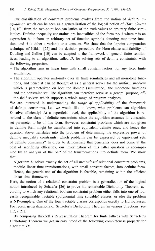
the running times. The programs are run on a HP9000=735 and timed using the ‘time’command. The compiler is the HP C compiler, using standard optimization (-O).The results for the 3-point lattice using the algorithm in Appendix A is shown in
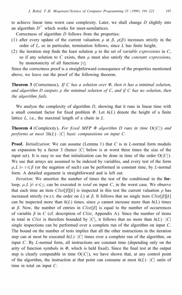
Fig. 1. Timings for the same constraint sets when translating to Horn-clauses is shownin Fig. 2. Timings for the 5-point lattice is shown in Fig. 3.

216 J. Rehof, T.�. Mogensen / Science of Computer Programming 35 (1999) 191–221
Fig. 1. Running times for algorithm D on 3-point lattice.
Fig. 2. Running times for algorithm D on 5-point lattice.
Fig. 3. Running times for 3-point lattice when translating to Horn clauses.
The results show a lightly more than linear increase in running time, but this canbe explained by an increase in cache misses when the data sets grow. For the con-straints used in the test, the methods solve roughly 100 000 constraints per second.This is fast enough that the problem is not time, but space. Roughly 30 bytes are used

J. Rehof, T.�. Mogensen / Science of Computer Programming 35 (1999) 191–221 217
per constraint in the current implementation, so solving a million constraints can bedone in 11 s, but it uses about 30MB of memory, most which is randomly accessed.This makes the wall-clock time increase dramatically when the data set size exceedsthe available physical memory, as swapping dominates. While constraints over the3-point lattice show little di�erence in time when solved by translation to Horn-clauses,the latter uses roughly twice as much memory, which makes it less practical for largedata sets. This will be even more of a problem when larger lattices or higher-arityoperators are used.The space problem can to an extent be reduced by using incremental versions of the
algorithm. It is fairly easy to modify the algorithm to keep a minimal solution whichis incrementally updated as more constraints are added. If a variable reaches the topof the lattice, all constraints with the variable on the right-hand side can be removedfrom the constraint set, as no monotonic changes can cause these to be unsatis�ed.The worst-case space cost is, however, unchanged, as variables may never reach thetop element of the lattice.
8. Conclusion
We have studied e�cient solution methods for the following classes of constraintproblems over �nite meet-semilattices:– De�nite inequalities involving monotone functions.– Distributive inequalities.– Boolean inequalities (Horn clauses).– Meet-closed relational constraints.We have shown that these classes are equivalent modulo linear time transformations forany �xed problem, and we have estimated the constant factors involved. For any �xedlattice and any �xed set of function=relation symbols the methods are linear time in thesize of the constraint set, but, in the case of boolean representation, the time dependsnon-linearly on the maximal arity of relation symbols used, and memory consumptionmay become rather large. Boolean representation should therefore be used only whenarities of functions involved are known to be small.We have characterized the expressiveness of the framework of de�nite constraints,
and we have shown that this framework captures a class of problems which is maximal,in the sense that adding any non-meet-closed relation to any non-trivial problem yieldsNP-hard uniform problems.
Acknowledgements
We wish to thank Fritz Henglein, Neil Jones, Helmut Seidl, Mads Tofte and ourreferees for helpful discussions and comments.

218 J. Rehof, T.�. Mogensen / Science of Computer Programming 35 (1999) 191–221
Appendix A. Algorithm
We assume the following structures and operations, together with some invariantproperties these items are required to satisfy:(1) A list Ilist of records representing the inequalities in C, the given de�nite con-
straint set; there is one record for each inequality in C. Each record holds a pointerto an inequality record in addition to the inequality itself. Each record also holds aboolean variable, called inserted. The intention is that the records in Ilist can be in-serted into a structure called NS (see below), and the �eld inserted must be set to true,if the inequality represented by the record is inserted in NS; it must be set to false,if the record is not in NS. The operations POP, INSERT and DROP (for which see below)will update the inserted �eld.(2) An array Clist[�] indexed by variables in Var(C). Each entry Clist[�] holds an
array of pointers to inequalitites in Ilist, one entry for each inequality in C in which� occurs. Thus, to each item in Clist[�] there corresponds a unique occurrence of �in C. Hence, the number of distinct items Clist[�][k] is bounded by |C|. Moreover,for each inequality in Cvar there is at least one entry in Clist pointing to it.(3) The structure NS is a doubly linked list of pointers to inequalitites in Ilist.
Pointers in NS point only to inequalities in Ilist which are among the inequalities inCvar, i.e., only those inequalities in Ilist which have a variable on the right-hand sidecan be pointed to by an element in NS. Each inequality in Ilist is represented by atmost one item in NS, but it may be the case that items in Ilist are not represented inNS. Each pointer in NS points to the item in Ilist which it represents, and that item inIlist has its pointer set to the representing item in NS. There is a pointer to the headelement of NS. The idea is that NS holds pointers to those inequalities in Cvar whichare not satis�ed under the current interpretation � (see below.)(4) A �nite map � mapping each distinct variable of C to an element in L. The
map � holds the current “guess” at a satisfying valuation for Cvar. The map ⊥Var(C)→ L
is the map which sends every variable of C to the bottom element of L. The map� is implemented as an array of lattice elements indexed by the variables. We write�(�) for �[�]. Evaluating �(�) is a constant time operation, and so is the operation ofupdating � at �, meaning that �(�) is changed into some new constant of L.(5) An operation POP which removes the head element of NS and returns it (i.e.,
POP returns a pointer to an inequality in Ilist.) Operation POP sets the inserted �eld tofalse in the inequality record in Ilist represented by the popped element of NS. Thisis a constant time operation (since there is a pointer to the head element of NS whichis maintained by POP).(6) An operation INSERT(i) which inserts an inequality pointer i at the front of NS.
Here i is an inequality pointer in Clist, and it is assumed that INSERT �rst checks to seeif the ag inserted associated with the Ilist-element pointed to by i is set to true. Ifthis is the case, then insert does nothing. If the ag is set to false, then INSERT sets the ag inserted to true, and then it inserts the pointer in the front of the list NS, updatingthe head pointer of NS. This is a constant time operation.

J. Rehof, T.�. Mogensen / Science of Computer Programming 35 (1999) 191–221 219
Fig. 4. Algorithm D for satis�ability of de�nite constraints over �.
(7) An operation DROP(i), where i is a pointer to an element of NS. Here i is aninequality pointer in Clist, and DROP �rst checks to see if the ag inserted associatedwith the inequality in Ilist pointed to by i is set to true; if this is the case, then DROP
removes the pointer from NS, and if the ag inserted is set to false, then DROP doesnothing. This is a constant time operation (since NS is a doubly linked list.)(8) An operation L-NORMALIZE which transforms a de�nite set into L-normal form.
This operation can be assumed to run in time O(|C|), and the size of L-NORMALIZE(C)is O(|C|), by Lemma 1. Moreover, solving L-NORMALIZE(C) is equivalent to solving C,by Lemma 2.In the algorithm we have followed the convention of writing the pattern of an
inequality pointed to by an inequality pointer instead of the pointer itself. Thus, theoperation �6� := POP(NS) is a shorthand for popping a pointer to the inequality �6�from NS and loading that pointer into a temporary variable while at the same timepulling the inequality (pointed to by the pointer) apart by pattern matching. This allcomes down to leaving a few indirections and a simple form of analysis of inequalitiesimplicit, in passing from elements in Clist t elements in Ilist and in NS. Also, inthe for-loop the pattern �6 is really a pointer to an element of Ilist containing theinequality �6 . Likewise, the set notation for the initialization of NS really means thatNS is initialized to a doubly linked list of pointers to the inequalities of C satisfyingthe condition of the set.

220 J. Rehof, T.�. Mogensen / Science of Computer Programming 35 (1999) 191–221
References
[1] T. Amtoft, Local type reconstruction by means of symbolic �xed point iteration, in: Proc. 5th EuropeanSymp. on Programming (ESOP), Edinburgh, Scotland, Lecture Notes in Computer Science, Vol. 788,Springer, Berlin, April 1994, pp. 43–57.
[2] C. Beeri, P. Bernstein, Computational problems related to the design of normal form relation schemes,ACM Trans. Database Systems (TODS) 4 (1) (1979) 30–59.
[3] L. Birkedal, M. Tofte, M. Vejlstrup, From region inference to von Neumann machines via regionrepresentation inference, in: Proc. 23rd Annual ACM Symp. on Principles of Programming Languages(POPL), ACM Press, New York, January 1996, pp. 171–183.
[4] L. Birkedal, M. Welinder. Binding-time analysis for Standard ML, Lisp and Symbolic Comput. 8 (3)(1995) 191–208.
[5] A. Bondorf, J. J�rgensen, E�cient analyses for realistic o�-line partial evaluation, J. Funct. Programming3 (3) (1993) 315–346.
[6] C.C. Chang, H.J. Keisler, Model Theory, Studies in Logic and the Foundation of Mathematics, 3rdEdition, Vol. 73, North-Holland, Amsterdam, 1990.
[7] N. Creignou, A dichotomy theorem for maximum generalized satis�ability problems, J. Comput. SystemSci. 51 (3) (1995) 511–522.
[8] B.A. Davey, H.A. Priestley, Introduction to Lattices and Order, Cambridge Mathematical Textbooks,Cambridge University Press, Cambridge, MA, 1990.
[9] R. Dechter, J. Pearl, Structure identi�cation in relational data, Arti�cial Intell. 58 (1992) 237–270.[10] William F. Dowling, Jean H. Gallier, Linear-time algorithms for testing the satis�ability of propositional
horn formulae, J. Logic Programming 3 (1984) 267–284.[11] D. Dussart, F. Henglein, C. Mossin, Polymorphic recursion and subtype quali�cations: polymorphic
binding-time analysis in polynomial time, in: Proc. 2nd Internat. Static Analysis Symp. (SAS), Glasgow,Scotland, Lecture Notes in Computer Science. Springer, Berlin, September 1995.
[12] T. Feder, M.Y. Vardi, Monotone monadic SNP and constraint satisfaction, in: 25th Annual Symp. onthe Theory of Computing (STOC), ACM, New York, 1993, pp. 612–622.
[13] M. Garey, D. Johnson, Computers and Intractability – A Guide to the Theory of NP-Completeness,Freeman, New York, 1979.
[14] R. Greenlaw, H.J. Hoover, W. Ruzzo, Limits to Parallel Computation. P-Completeness Theory, OxfordUniversity Press, Oxford, 1995.
[15] F. Henglein, E�cient type inference for higher-order binding-time analysis, in: J. Hughes (Ed.),Functional Programming Languages and Computer Architecture, Cambridge, Massachusetts, August1991, Lecture Notes in Computer Science, Vol. 523, ACM, Springer, Berlin, 1991, pp. 448–472.
[16] F. Henglein, Iterative �xed point computation for type-based strictness analysis, in: BaudouinLe Charlier (Ed.), 1st Internat. Static Analysis Symp. (SAS), Namur, Belgium, Lecture Notes inComputer Science, Vol. 864, Springer, Berlin, September 1994, pp. 395–407. Also DIKU SemanticsReport D-192.
[17] W. Hodges, Model Theory. Encyclopedia of Mathematics and its Applications, Vol. 42, CambridgeUniversity Press, Cambridge, 1993.
[18] P. Jeavons, M. Cooper, Tractable constraints on ordered domains, Arti�cial Intell. 79 (1995) 327–339.[19] P. Jeavons, D. Cohen, An algebraic characterization of tractable constraints, in: First Annual Conf. on
Computing and Combinatorics (COCOON), Lecture Notes in Computer Sciences, Vol. 959, Springer,Berlin, 1995, pp. 633–642.
[20] P. Jeavons, D. Cohen, M. Gyssens, A unifying framework for tractable constraints, in: 1st Internat.Conf. on Principles and Practice of Constraint Programming, Lecture Notes in Computer Sciences,Vol. 976, Springer, Berlin, 1995, pp. 276–291.
[21] S. Khanna, M. Sudan, D.P. Williamson, A complete classi�cation of the approximability of maximizationproblems derived from boolean constraint satisfaction, in: Proc. 29th Annual ACM Symp. on Theoryof Computing (STOC), ACM, New York, May 1997.
[22] G. Kildall, A uni�ed approach to global program optimization, in: Proc. ACM Symp. on Principles ofProgramming Languages (POPL), 1973.
[23] T.�. Mogensen, Types for 0, 1 or many uses, in: Proc. 9th Internat. Workshop on Implementation ofFunctional Languages, St. Andrews, Scotland, September 1997.
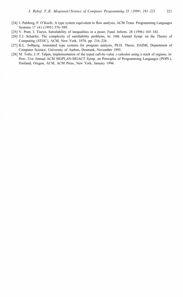
J. Rehof, T.�. Mogensen / Science of Computer Programming 35 (1999) 191–221 221
[24] J. Palsberg, P. O’Keefe, A type system equivalent to ow analysis, ACM Trans. Programming LanguagesSystems 17 (4) (1995) 576–599.
[25] V. Pratt, J. Tiuryn, Satis�ability of inequalities in a poset, Fund. Inform. 28 (1996) 165–182.[26] T.J. Schaefer, The complexity of satis�ability problems, in: 10th Annual Symp. on the Theory of
Computing (STOC), ACM, New York, 1978, pp. 216–226.[27] K.L. Solbjerg, Annotated type systems for program analysis, Ph.D. Thesis, DAIMI, Department of
Computer Science, University of Aarhus, Denmark, November 1995.[28] M. Tofte, J.-P. Talpin, Implementation of the typed call-by-value �-calculus using a stack of regions, in:
Proc. 21st Annual ACM SIGPLAN-SIGACT Symp. on Principles of Programming Languages (POPL),Portland, Oregon, ACM, ACM Press, New York, January 1994.


