Embed Size (px)
Citation preview
Traffic ControlDevices, Geometrics,Visibility, andRoute Guidance
TRANSPORTATION RESEA RCH BOARD
COM M ISS/ON ON SOC/ OTECH N I CAL SYSTEMSNATIONAT RESEA RCH COUNCIL
NATIONAL ACADEMY OF SC/ENCESWASHINGTON, D.C. 1979 ,i,
Transportation Research Reeord 737Price $6.60Edited for TRB by Amy E. Shaughnessy and Brenda J, Vumbaco
Sponsorship of the Papers in This Transportation Research Record
GROUP 3-OPERATION AND MAINTENANCE OF TRANSPORTA.
modes TIOILEÁ,CILIÏIES
r hþhway transportation Adorf D. May, university of &riþmia, Berkerey, chairman
3 rail transportation Committee on Traffic Control Devices
subject areas52 human facto¡s54 operations and traffic control
Transportation Research Board publications are available by order-ing directly f¡om TRB. They may also be obtained on a regularbasis through organizational or individual alfiliation with TRB; af-filiates or Library subscribers are eligible for substantial discounts.For fu¡ther information, write to the Transportation Resea¡chBoard, National Academy of Sciences, 2101 Constitution Avenue,N.W., Washington, DC 20418.
NoticeThe papers in this Record have been teviewed by and accepted forpublication by knowledgeable persons other than the authors ac-cording to procedures approved by a Report Review Committeeconsisting of members of the National Academy of Sciences, theNational Academy of Engineering, and the Institute of Medicine.
The views expressed in these papers are those of the authorsand do not necessarily reflect those of the sþonsoring committee,the Transportation Research Board, the National Academy ofSciences, ot tlte sponsors of TRB actvities.
Library of Congress Cataloging in Publication DataNational Research Council. Transportation Research Board.
Traffic control devices, geometrics, visibility, and route guid¿nce.
(Transportation research rcco¡d,; 7 37)1. Electronic traffÏc controls-Addresses, essays, lectures,
2. Roads-Lighting-Addresses, essays, lectures. 3. Roads-Inter-changes and intersections-Design and construction-Addresses,essays, lectures. 4. T¡affic safety-Addresses, essays, lectures.I. Title. II. Series.
lEl.Hs yo.737 [TE228] 380.5s l6zs.7'941 8G17s43ISBN 0-309-02992-9
Ken F. Kobetsky, West Virginia Deryrtment of Highwøys, chairmtnH, Milton Heywood, Federal Highway Adminisfføtion, IecretaryIohn L. Barker, Robert L. Bleyl, Edward L. Cook, Charles E. Dare,J. R. Doughty, Thomts I. Foody, Paul H. Fowler, Robert M.Garrett, Alan T. Gonseth, Robert L. Gordon, Gerhart F. King,Kay K, Krekorian, Hugh Ilt. McGee, Robert D. McMillen, Ioseph A.Mickes, Zoltøn A. Nemeth, Harold C. Rhudy, fohn C. Rice, DavídG. Snider, Ronald E. Stemmler,,Iames L Tøylor, James A. Thomp-son, Thomas L. Vønvechten, Clinton A, Venøble, Earl C. l4tittiamífr,, l4/alter P. Youngblood, Jason C. Yu
Committee on VisibilityNathaniel H. Pulling, Libefty Mutuøl Reseørch Center, chairmanSamuel P. Sturgís, Liberty Mutual Research Center, secretaryAlbert Burg, Charles l4t. Oøig, Warren H. Edrn¿n, Ralph A.'Ehrhardt, Eugene Farber, W, S, Fanell, T, lU. Forbes, Vincent p.Gallagher, S. A, IIeenan, Robert L. Henderson, Clarles H. Kaehn,Antan¿s Ketvirtis, Lee Ellß King, Ken F. Kobetsky, Ralph R. I¿u,Richørd N. Schwab, Richørd E. Stark, Ftederick E. Vanosilall,Ned E. l4talton, Eørl C. h)illiams, Jr., Ítlilli¿m L. 't4tüiams, Henry L.Woltman, Kenneth Zied man
Committee on Railroad-Hþhway Grade CrossingsOtto F. Sonefeld, Atchison, Topeka and Santa Fe Railwøy
Company, chairmanH?ward C, Palrner, Søfetran Systems Corporation, secretaryCharles L. Amos, WilliomD. Berg, Lucien M. Boton, Archie C,Burnham, Ir., Louis T. Cerny, Janet A. Coleman, Bruce F. George,Bruce Lanier Gordon, llillíam J. Hedley, John Bradford Hopkins,Robert C. Hunter, Robert A, Lavette, Richard A. Mather, G. RexNichelson, Jr., Hoy A. Richards, Eugene R. Russell, C, Shoemaker,Max R. Sproles, Barry M. Sweedler, Richørit A. Wüto
Committee on Operational Effects of GeometricsStanley R. Byington, Federal Híghwøy Administtation, chairman4obert B. Helland, Federal Highway Administrøtion, secretaryFrank E, Barker, Robert E. Ctøven, Edwin ll). Dayton, f, GknnEbersole,Ir., Daniel B, Fambro,,Iulie Anna Fee,Iohn Feolø,John C. Glennon, George F. Høgenauer, Raiendra Jain, Janis H.I¿cis, William John Laubøch,.Ir., Lltittiam A. McConnell, WoodrowL, Moore, f,r., Robert P. Morris, Thomøs E, Mulirazzi, SheldonSchumacher, Jømes f. Schuster, Robert B. Shaw, C, RobertShinhøm, Bob L. Smith, Robert C. iltin¿ns
Committee on Traffic Flow Theory and CharacteristicsKenneth I4t. Oowley, Pennsylvønio State University, chairmanMmund A. Hodgkins, Federal Highway Administration, secretatyCþrles R, Berger, Said M. Easa, Iohn W Erdman, Antranig V.GaførÍan;Nathan H. Gartner, f,ohn L Haynes, F-ichard L.EõEiltge4ryqtthew f. Huber, Iohn B. Kreer, Joseph K. Lam, Tenny N. I"øm,E_dward B. Lieberman, Roy C. Loutzenheiser, Canott L'Messer,Pøul Ross,_Richard Rothery,Ioel Schesser, Steven R, Shapùo,A. D. St. John, W. ll. lilolman
Committee on User Information Systemsl4tøllace G. Berger, U.S. Senate Appropriations Commíttee,
chairmanFre d R. Ha n sco m, B io Te chno lo gy, In c., se ø e taryTerrence M. Allen, Hebert J. Bøuer, Normøn J. Cohen, Koren p,Damsgaard, Robert Dev)ar, f. Gþnn Ebersole, fr., Eugene Føber,Iohn C. Hayward, Robert S, Hostetter, Gerhørt F. King, HatoldLunenfeld, Truman Mast, Peter B. Moreland, Theodore J. post,Martin L. Reiss, Arthur W. Roberts III, Bob L. Smith, Eugeræ M.I4)ilson
David K. Witheford and James K. Williams, Transportation ResearchBoard staff
Sponsorship is indicated by a footnote at the end of each report.The organizational units and officers and members are as ofDecember 31,L978.
C ontents
WARRA}TTS FOR LEFT-TURN SIGNAL PHASINGKenneth R. Agent and Robert C. Deen . . . . . , 1
GUIDELINES ¡OR TRAFFIC COI.ITROL AT ISOLATEDINTERSECTIONS ON HIGH-SPEED RURAL HIGHWAYS
Ahmed Essam Radwan, Kumares C. Sinha, andHaroldl,Michael ....10
USE OF EC-DC DETECTOR FOR SIGNALIZATION OFHIGH -SPEED I}ITERSE qTIONS
Peter S. Parsonson, Richard A. Day, James A. Crawlas,andGeorgeW.Black,Jr.... .,,,..L7
MAI}ITENANCE COSTS OF TRAFFIC SIGNALSPeter S. Parsonson and Philip J. Tarnoff . , . 24
REFLECTORIZATION OF RAILROAD ROLLING STOCKRichardG.McGinnis .......31
DiscussionLouisÎ.Cerny. ..,..40JohnB.Hopkins .....40OttoF.Sonefeld .....4L
Author'sClosure .......42ACCIDETTT AND OPERATIONAL GUIDELINES FORCO}ITINUOUS TWO-WAY LE T'T-TURNMEDIAN LANES
C. Michael Walton, Randy B. Machemehl, Thomas Horne,andWilliamFUng.. ...43
DiscussionStanleyl.Ring ......52JohnC.Glennon .....53ZottanA.Nemeth ....53
BENEFIT-COST ANALYSIS OF ADVANCE TREATMENTFoR NO-PASSING ZONES G¡ri¿gment)
Donald L. Woods and Graeme D. Weaver . , . . 5õ
SHOULDER IMPROVEME}ÍTS ON TWO-LANEROADS G,uriagment)
Davidl. Davis. ...... 59
MODERN ROTARIES: A TRANSPORTATION SYSTEMSMANAGEME}TT ALTERNATTVE
KennethTodd. ......61Discussion
G. F. Hagenauer . . ., . 68RobertJ.Noþn .,....69JackE. Leisch ......69
AuthorrsClosure .....,.70
ltl
IV
HIGHWAY GUIDE SIGNS: A FRAME\4/ORK FORDESIGN AND EVALUAÎION
J. Paul Dean. 72
FORMATION AND DISSIPATION OF TRAFFIC QUEUES:SOME MACROSCOPIC CONSTDERATIONS (Abridgment)
Panos G. Michalopoulos, Vijay B. pisharody,George Stephanopoulos, and GregoryStephanopoulos . . . . . . . . . g1
DISCOMFORT GLARE: A REVIEW OF SOME RESEARCH(Abriogment)
CorwinA. Bennett ....... g4
ECONOMIC MODELS FOR HIGHWAY AND STREETILLUMINATION DESIGNS
Richard W. Slocum and Daniel R. prabudy . . . , . . g6
TEST OF 4OO-W HIGH-PRESSURE SODIUM VAPORLIGHTING (Abridgment)
MichaelC.Belangie ....,.91PAVEMENT INSET LIGHTS FOR USE DURING FOG(Abridgment)
FrankD.Shepard .......98DRIVER PERFORMANCE WIÎH RIGHT-SIDE CONVEXMIRRORS
Ronald R. Mourant and Robert J. Donohue . . . . . . gbDiscussion
ThomasH.Rockwell .....101Robert L. Henderson . . .. . . . . . ,101Rudolf G. Mortimer ..,,..l)zAuthorstClosure . ....104
HI]MAN FACTORS CONSIDERATIONS FOR IN-VEHICLEROUTE GUIDANCE
Conrad L. Dudek . . .LOA
FEASIBILTTY STUDY OF ROUTE GIIIDANCE SYSTEMF\rmihiko Kobayashi .. .. ..10?
OÜTLINE OF THE COMPREHENSryE AIITOMOBILETRAFFIC CO}I"TROL PILOT TEST SYSTEM
Nobuo Yumoto, Hirokazu Ihara, Tsutomu Tabe, andMasaruNaniwada ...119
Warrants for Left-Turn Signal PhasingKenneth R. Agent and Robert c. Deef\ Division oI Hesearcnr lJureau ot
Highways, Kentucky Department of Transportation, Lexington
Warrants for the ¡nstallation of left-turn phasing in Kentucky were de-veloped. A review of the l¡terature was conducted, along with a surveyof the pol¡cies of other states. F¡eld data on-delays and conflicts weretaken before and after installat¡on of exclusive left-turn s¡gnalizat¡on.Left-turn delay studies were conducted at intersect¡ons that had vary¡ngvo¡ume condit¡ons. Analysis of the effect on accidents of adding a left-turn phase was made. The relationship between left-turn accidents andconflicts was ¡nvest¡gated. Other types of analyses concerning gap ac-
ceptance, capac¡ty, and benef¡t-cost rat¡os were also performed. lt wasfound that exclusive left-turn phasing significantly reduced left'turn ac-
cidents and conflicts. This reduction was offset in part by an increasein rear-end accidents. Left-turn delay was reduced only during periodsof heavy traffic flow, Total delay for an intersection increased after in'stallat¡on of left-turn phasing. Warrants were developed deal¡ng withaccident experience, delay, volumes, and traffic conflicts.
A vehicle attempting to turn left across opposing trafficis a common problem. Separate left-turn lanes mini-mize the problem but may not be the final solution. Atsignalized intersections, left-turn phasing can þe usedas an additional aid. Ho',vever, warrants have not beenestablished for the addition of separate left-turn lanesor signal phasing, In this study, warrants or guideswere developed for installing left-turn phasing at sig-nalized intersections that have separate left-turn lanes'Before-and-after data were taken at locations where left-turn phasing had been added. Studies at locations thathad varied traffic conditions were made to determinethe relationship between various volumes and left-turndelays. The relationship between left-turn accidentsand conflicts was investigated, Comparisons of sig-nalized intersections with and without left-turn signalswere also made.
SURVEY OF OTHER STATES
Other state highway agencies were requested to des-cribe their procedure used to determine the need forleft-turn phasing. Of the 45 states responding, only 6
cited numerical warrants for left-turn phasing. In one
state, warrants were proposed. The various numericalwarrants used when considering left-turn phasing wereas follows (some states had more than one warrant):
1l pã¿uct ot ttre tett- tui¡r nighe st- houi volumeand the opposing traffic > 50 000;
2. Five or more left-turn accidents within a 12-month period (two states);
3. Cross product of left turns and conflictingthrough peak-hour volumes >100 000 (two states, onelisting this for traffic-actuated signals only);
4. De1ay to left-turning vehicle in excess of twocycles;
5. One left-turning vehicle delayed one cycle ormore in t h;
6. At a pretimed signal, left-turn volume of morethan trvo vehicles per approach per cycle during a peakhour;
1. Average speed of through traffic exceeds 72
km/h (45 mph) and the left-turn volume is 50 or moreon an approach during a peak hour;
B. Left-turning volume exceeds 100 vehicles duringthe peak hour;
9. More than 90 vehicles,/h making a left turn; and10. For four-lane highways with left-turn refuges, a
relationship between left-turn volume, opposing-trafficvolume, and posted speed.
Nearly all of the responses listed guidelines that havebeen used. Following is a list of the general guidelines(areas that should be considered) that were mentioned,some of which were listed by several states: accidentex¡lerience, capacity analysis, delay, volume counts(peak-hour left-turn and opposing through volumes),turning movements, speed, geometrics, signal progres-sion (consistency with and effect on adjacent signals),queue lengths, right-of-way available, number of op-posing lanes to cross, gaps, consequences imposed onother traffic movements, type of facility, sight distance,and percentage of trucks and buses, Several states listedmore detailed guidelines involving specific left-turnvolumes, etc.
Following is a summary of guidelines used when con-sidering a separate left-turn signal phase: left-turnvolume > 500 (two-lane roadway), wherever a left-turnlane is installed on divided highways; 100-150 left-turning vehicles during the peak hour (small cities);150-200 left-turning vehicles during the peak hour (largecities); at new installations, where left-turn phases al-ready exist at other intersections on the same roadway;average cycle volume exceeds two vehicles turning leftfrom the left-turn bay, and the sum of the number ofleft-turning vehicles per hour and the opposing-trafficvolume per hour exceeds 600 vehicles; high percentageof left-turning vehicles (20 percent or greater); not pro-vided at intersections with left-turn volume < 80vehicles,/h for at least I h/day; the number of left-turning vehicles is about 2 per cycle; 120 left-turningvehicles in the design hour;.turning volume in excess of100 vehicles fh, and, more than one cycle of the signalneeded to clear a vehicle stopped on the red; left-turnvolumes of 90-120 in peak hours; and more than 100turns/h.
RESULTS
Accident rffarrant
Bef ore- and-After Accident Studies
Accident data before and after installation of separateleft-turn phasing were collected for 24 intersections'The length of the before and after periods was usuallyone year, but it varied in some cases depending onthe available data. There was an 85 percent reductionin left-turn accidents, defined as those occurring whenone vehicle turned left into the path of an opposingvehicle. This reduction in left-turn accidents was off-set in part by a 33 percent increase in rear-end acci-dents. There was a reduction of 15 percent in totalaccidents.
Accident severity was reduced only slightly afterinstallation of the left-turn phasing. Rear-end acci-dents (which were increased) are less severe than left-turn (angle) accidents (which were decreased). Injuryaccidents decreased from 13 to 11 percent after left-
2
turn phasing uras installed.
Comparison of Accident Rates at
For P = 0.995, the critical number of left-turn acci-dents per year p'er approach was found to be four. Usingthe high probability increases the likelihood of selecting
Left-Turn Phasing left-turn probleín. Therefore, four left-turn accidentsin one year on an approach would make that approach
Accident rates at intersections in Lexington, Kentucky, critical. The number of accidents in a two-year periodwith and without left-turn phasing were compared. Rate necessary to make an approach critical was also deter-were calculated by using 1972 accident data, and the vol- mined. There was an approximate average of two left-ume data were taken for 19?1 through 1973. Volume turn accidents on an approach during a two-year period.counts were available for a 12-h period (?:00 a. m. to By using this average of two accidents, the numbãr of7:00 p' m. ) at each intersection. The assumption was lelt-turn accidents necessa"y tn
" ¡*6-year period to
made that 80 percent of the total daily volume occurred make an approach critical was found to be six.in this 12-h period, so the volumes were multiplied by The same procedure was used to determine the1.25 to obtain the 24-h volume. The total rate of the critical number of accidents for both approaches whenintersection-type accidents was computed in terms of a street has left-turn lanes in both directions. Foraccidents per million vehicles entering the intersection. 1968 through 19?2, the average number of left-turn ac-The left-turn accident rate was calculated, for each ap- cidents for both approaches on a street was 2.1 (for 36proach that had a separate left-turn lane, in terms of streets with left-turn lanes for both directions at anleft-turn accidents per million vehicles turning left from intersection but no separate phase). This resulted in athe approach. Interseetions without left-turn phasing critical number of 6 for a one-year period for both ap-(44 intersections) had average annual daily traffic proaches. For a two-year period, án average of 4(AADT) of approximately 20 000, compared with slightty accidents resulted in a critiial number of 10 for bothmore than 32 000 for intersections that had left-turn approaches.phasing (16 intersections). The higher AADT affectsthe accident rate. Calculating rates for only the high- Delay Warrantvolume intersections (AADT > 25 000) eliminated thisvariable. There were 13 intersections that had sepa- Before-and-After Delay and Conflictrate phasing and 10 intersections without separate Studiesphasing that met this criterion.
The left-turn accident rate was drastically lov¿er for To determine the change in vehicular delay, studiesthe approaches that had left-turn phasing (0.77 left-turn were conducted before and after installation of left-turnaccidents/mÍllion vehicles entering the intersection for phasing at three intersections that had two-phase, semi-all intersections, 0.86 for high-volume intersections) actuated signalization. Left-turn delay was defined asthan for approaches without left-turnphasing (2.741or the time from whenthe vehicle arrived inthe queue orall intersections and 3.?6 for high-volume intersections). at the stop bar until it cleared the intersection. TheThe lower rate agreed with the findings of the before- arrival and departure times of each left-turning vehicleand-after accident studies. The data again showed that were noted; delay could then be calculated. If theleft-turn phasing did not reduce the total intersection vehicle did not have to stop, a zero delay was noted.accident rate. The total accident rate was almost iden- The number of left turns was counted. Opposing vol-tical at locations with (1.66 for aII intersections and umes and left-turn conflicts were also counted during1.63 for high-volume intersections) and without (1.63 the study period, usually 30 min of each hour.for all intersections and 1.69 for high-volume inter- Because of high volumes involved when determiningsections) left-turn phases. total intersection delays, the stop-type delay, the time
in which the vehicle is actgally stopped, was used be-Critical Left-Turn Accident Number cause it was the easiest and most piactical delay to
measure (2, 3). The estimating procedure consisted ofBy using the Lexington data base, the average number counting the number of vehicles stopped in each inter-of left-turn accidents for the approaches with no left- section approach at periodic intervals. The intervalturn phasing was calculated. By using this average used was 15 s for two of the intersections and 20 s fornumber of accidents, the crilical number of accidents the other. The volume on eaqh 4pplqaSb w4C 4LSSwas also determined. Foi 1968 through 19?2, ttre cointè¿. The total ct.lay w-s ttrelro¿uit of tne totataverage number of left-turn accidents per approach was vehicles stopped at periodic intervals and the length of0.93 (for 96 approaches with a left-turn lane but no the interval.
- The dèlay per vehicle was obtained-by
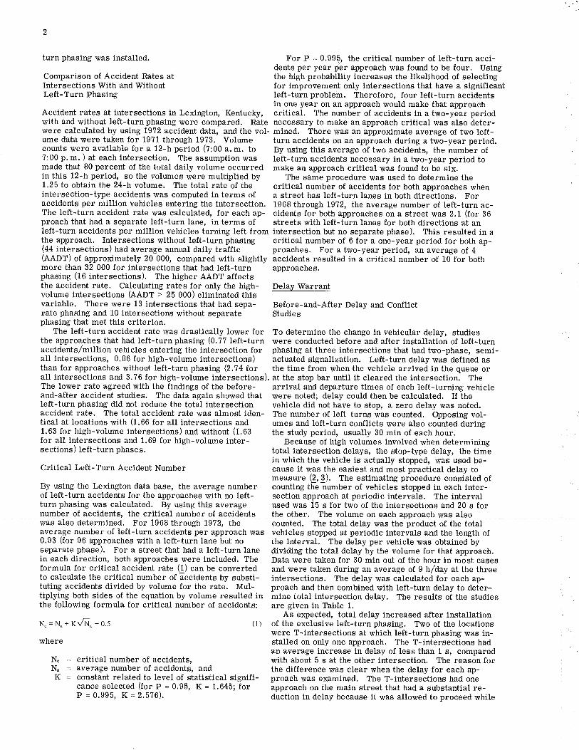
separate phase). For a street that had a left-turn lane dividing the total delay'by the volume for that appròach.in each direction, both approaches were included. The Data were taken for 30 min out of the hour in most casesformula for critical accident rate Q) can be converted and were taken during an average of.9 h/day at the threeto calculate the critical number of ãccidents by substi- intersections. The dãlay was câIculated for each ap-tuting accidents divided by volume for the rate. Mul- proach and then combined ryith left-turn delay to deter-tiplying both sides of the equation by volume resulted in mine total intersection delay. The results of the studiesthe following formula for critical number of accidents: are given in Table 1.
As expected, total delay increased after installationN. = N^ + rr,fiq + o.s (1) of the exèlusive left-turn pirasing. Two of the locations
were T-intersections at which left-turn phasing was in-where stalled on only one approach, The T-intersections had
an average increase in delay of less than 1 s, comparedN" = critical number of accidents, with about 5 s at the other intersection. The reason forNe = average number of accidents, and the difference was clear when the delay for each ap-K = constant related to level of statistical signifi- proach was e><a.mined, The T-intersections had one
cance selected (for P = 0.gS, K = 1.645; for ãpproach on the main street that had a substantial re-P = 0.995, K = 2.5?6). duction in delay because it was allowed to proceed while
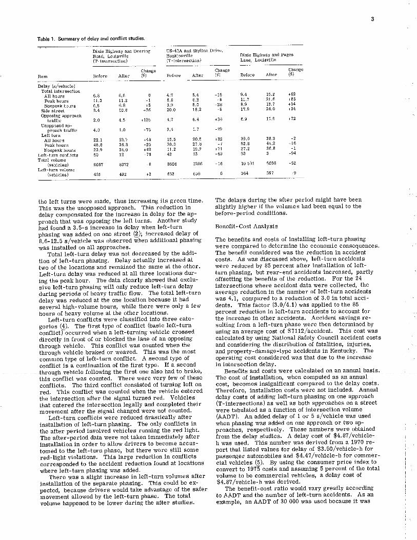
Table 1. Summary of delay and conflict stud¡es.
Dixie Highway and Deering US-414 and Skyline D¡ive'Ilopkinsville Dixie Highway and Pages
ChangeBefore After (í\
ChangeAfter $)
changeAfter $)
Delay (s/vehicle)Total intersection
AII hoursPeak hoursNonpeak hours
Side streetOpposing approach
trafficUnopposed ap-
proach trafficLett turnAII hou¡sPeak hoursNonpeak hours
Left-turn conflictsTotal volume
(vehicles)Left-turn volume
(vehicles )
6.811.36.58.4
2.0
4.0
22.148.823.950
905?
481
6.8Lt.26.810.6
4.5
1.0
32.',t36.834.072
8372
492
0-1r5
+26
+125
4.16.83.920.0
4.7
2.4
15.530.011.242
5.46.25.078.2
6.4
7.7
20.5
19.213
7208
650
+15-9
+28-9
+36
-29
+32
+?1-69
-16
0
-75
+48-25+42-?6
-8
+2
8606
653
9.4 t5.2 +6211.? 21.6 +858.9 13,7 + 541?.9 24,O +34
6.9 11.9 +72
39.0 38.3 -252.8 44.2 -1637.2 36.8 - I53 3 -94
10 531 5036 -52
364 39? +9
the left turns were made' thus increasing its green time'This was the unopposed approach. This reduction indelay compensated for the increase in delay for the ap-proach that was opposing the left turns' Another studyhad found a 3.5-s increase in delay when left-turnphasing was added on one street (?); increased delay of8.6-12.5 s/vehicle was observed when additional phasÍngr¡ùas installed on all approaches.
Total left-turn delay was not decreased by the addi-tion of left-turn phasing. Delay actually increased attwo of the locations and remained the same at the other.Left-turn delay was reduced at all three locations dur-ing the peak hour. The data clearly showed that exclu-sive left-turn phasing will only reduce left-turn delayduring periods of heavy traffic flow' The total left-turndelay was reduced at the one location because it had
several high-volume hours, rvhile there were only a fewhours of heavy volume at the other locations'
Left-turn conflicts'üere classified into three cate-gories (4)' The first type of conflict (basic left-turnconflictfoccurred when a left-turning vehicle crosseddirectly in front of or blocked the lane of an opposingthrough vehicle. This conflict was counted when thethrough vehicle braked or weaved' This was the mostcommon type of left-turn conflict. A second type ofconflict is a continuation of the first type. If a second
Jh+ough vehicle following the firslone alsoha-d Lo þrake'this conflict was counted' There were very fe"v of theseconflicts. The third conflict consisted of turning left onred, This conflict was counted',vhen the vehicle enteredthe intersection after the signal turned red. Vehiclesthat entered the intersection legally and completed theirmovement âfter the signal changed were not counted.
Left-turn conflicts were reduced drastically afterinstallation of left-turn phasing' The only con-flicts inthe after period involved vehicles running the red light.The after-period data were not taken immediately afterinstallation in order to allow drivers to become accus-tomed to the left-turn phase, but there were still somered-light violations. This large reduction in conflictscorresponded to the accident reduction found at locationswhere left-turn phasing lt¡as âdded.
There was a slight increase in left-turn volumes afterinstallation of the separate phasing. This could be ex-pected, because drivers would take advantage of the safermovement allowed by the left-turn phase. The totalvolume happened to be lower during the after studies.
The delays during the after period might have beenslightty higher if the volumes had been equal to thebefore-period conditions.
Benefit-Cost Analysis
The benefits and costs of installing left-turn phasingwere compared to determine the economic consequences.The benefit considered was the reduction in accidentcosts, As was discussed above' left-turn accidentswere reduced by Bb percent after installation of left-turn phasing, but rear-end accidents increased, partlyoffsetting the benefits of the reduction. For the 24intersections where accident data were collected' theaverage reduction in the number of left-turn accidentswas 4.1, compared to a reduction of 3.0 in total acci-dents. This factor (3.0/4,1) was applied to the 85percent reduction in left-turn accidents to account forthe increâse in other accidents. Accident savings re-sulting from a left-turn phase were then determined byusing an average cost of $?112,/accident. This cost wascalculated by using National Safety Council accident costsãnd considering the distribution of fatalities, injuries'and property-damage-type accidents in Kentucky' Theoperating cost considered was that due to the increasein intersection delay.
ienelits a¡d clsts were calqulated on an a¡4uall4$qtThe cost of installation, when computed as ân annualcost, becomes insignificant compared to the delay costs.Therefore, installation costs were not included. Annualdelay costs of adding left-turn phasing on one approach(T-intersections) as well as both approaches on a streetv/ere tabulated as a function of intersectÍon volume(AADT). An added delay of 1 or 5 s/vehicle was usedwhen phasing was added on one approach or two ap-proaches, respectively. These numbers were obtainedirom the delay studies. A delay cost of $4.8?/vehicle-h was used. This number ¡¡¿as derived from a 19?0 re-port that listed values for delay of. $3.5O/vehicle-h forpassenge" automobiles and $4.41 /vehicle-h for commer-cial vehicles (5). By usÍng the consumer price index toconvert to 1975 costs and assuming 5 percent of the totalvolume to be commercial vehicles' a delay cost of$4. 8?/vehicle-h was derived.
The benefit-cost ratio would vary greatly accordingto AADT and the number of left-turn accidents. As ane)<a.mple, an AADT of 30 000 was used because it was
4
close to the average volume for the Lexington inter- approximating ?3 s, this ratio was about 1.b. By usingsections that had left-turn phases. This would result this ratio, a value of 35 s for the mean delay waä det"i-in an annual delay cost of $14 800 and $?4 100 for add- mined. This value of 35 s was used as the minimuming phasing to one and two apprn¡ehes, respectively. average clelay¡ecessary, sinee this eonstituted theThe critical number of left-turn accidents in one yearwas used to determine accident savings. For a T-intersection, the critical number of four yields an an-nual savings of $17 ?00. The benefit-eost ratio wouldbe 1.20, For two approaches, the critical number is
lower bound of excessive delay.When considering what would constitute excessive
delay, the delay to left-turning vehicles turning only onthe amber phase was calculated. This would approxi-mate peak-flow conditions when the only gap available
six' which gives an accident savings of $26 500. Using to turn left occurs at the end of the amber phase. Thethe delay cost of $74 100 yields a benefit-cost ratio of maximum delay possible if none of the vehiìles had to0.36. wait more than one cycle length was determined. The
As a general ru1e, the savings attributable to acci- maximum delay possible would occur when the left-dent reduction should offset the increased cost due to turning vehicle arrived at the start of the red phase anddelay when street geometry makes left-turnphasing departed during the amber phase. This delayiould benecessary on only one approach that has a critical approximately equal to oneìycle. The numb-er of ve-number of accidents. This situation would be approxi- hicles that could turn left in t h during the amber phasesmated if both approaches must be signalized but left- was dependent on the cycle length. Since peak-hoúr con-turn volume on one approach is very low. Since the ditions were specified, the assumption wai made thatleft-turn phasing would be actuated, this would approxi- side-street traffic would be heavy enough to make anmate the T-intersection situation if the left-turn phasing actuated signal behave as a fixedrtime signal with afor one approach was used only during a very small constant cycle length, If the cycle length were 60 s,percentage of the cycles. However, when a street has there would be 60 amber phases available to left-relatively high left-turn volumes on both intersection turning vehicles. Thirty amber phases would be avail-approaches' the cost of increased delay will be much able during the peak hour at a signal with a 120-s cycle .
higher than the savings from accident reduction. length. If an average of 1.6 vehicles turned left duiingeach phase of amber, 96 vehicles,/h could turn left if
Left-Turn Delay the cycle length were 60 s. This volume would decreaseto 4B/h for a cycle length of 120 s. For a maximum
Excessive delay in left turns is one of the major rea- delay of one cycle, the total delay for the peak hour wassons for installing separate left-turn signals. A good determined to be 1.6 vehicle-h for both cyèle lengthsdelay criterion should include both delay and volume. Field e><perience has shown that during peak conditionsMultiplying the average delay per vehicle (seconds) by the number of vehicles turning left duiing each phasethe corresponding left-turn volume yields the number of amber can become close to 2 if the left-turn volumeof vehicle-hours of delay. This unit of delay was used is heavy. If an average of 2 vehicles turn left duringin this study. Also, further safeguards were built into each amber phase, the total left-turn delay becomeJ2.0the delay warrant. Minimum delay per vehicle and vehicle-h during the peak hour. Delays in excess of theseminimum volumes were specified so that neither very values could be considered excessive. These delayslow volumes with excessive delays nor very high vol- would apply to the critical approach.umes with minimal delays would meet the warrant. Delay data collected at several intersections wereThe delay during peak-hour conditions was specified, compared with these values to check their validitysince these are the conditions that create excessive As stated earlier, studies were done before installationdelays' of left-turn phases at three intersections, During
Cycle time and the number of vehieles that might peak-hour conditions before installation, left-turn de-turn left during amber periods were considered when lays of 2,45, t.2'7, and 1.64 vehicle-h were found atdetermining a minimum left-turn volume. The maxi- those three locations. The location that had a delay ofmum cycle that normally would be used is 120 s. This 1.2? vehicle-h also had an average left-turn delay dur-would give 30 periods oÍ. amber/h for use by left-turning ing the peak hour of only 30 s, Six intersections invehicles. Assuming that a minimum average of 1.6 Lexington that had high left-turn delays were selectedvehicles could turn left during each amber phase, 48 for detailed delay studies, Delays were measured onvehicles,/h could turn left during amber undãr peak both streets at one of the intersections. Left-turnopposing-fJow eonditions- Therefore, a minimum left- delays were measured for several hours during the day.turn volume of 50 vehicles in the peak hour was speci- The peak-hour delay was > 2.0 vehicle-h (varying fromfied. 1.?6 to 5.96) in aII but one case. Only two of the critical
A minimum value necessary for the average left-turn approaches had peak-hour delays > 2.5 vehicle-h. Alldelay was also determined. Since installing a separate of these approaches met the criteria of minimum left-left-turn phase would increase total delay at the inter- turn delay and volume. The field data show that peak-section, the supposition was made that a minimum delay hour, left-turn delay in excess of 2.0 vehicle-h canwas necessary to left-turning vehicles independent of occur regularly at locations that have a left-turnthe left-turn volume. To determine this level of delay, problem.a past survey of engineers was used (6). This survey A review of the literatue (!) disclosed two peak-asked the engineers for their opinion õf wnat consti- hour delay warrants for the insta[ation of traffic sig-tuted maximum tolerable delay for a vehicle controlled nals that had been developed in terms of vehicle hoursby a traffic signal. A mean value of 73 s was found, of delay. One warrant requires that the average side-The criterion used was that 90 percent of all left-turning street vehicle delay in seconds multiplied by side-streetvehicles be delayed less than this maximum of ?3 s. volume per hour be equal to or exceed 8000. This is
Assuming that the distribution of delays was approxi- equivalent to 2.2 vehicle-h of delay. Another peak-hourmately normal, it was then possible to find the mean of delay warrant for a single, critical left-turn approachthe delay distribution whose 90th percentile value was was 2.0 vehicle-h of delay. A minimum volume of 100 i
approximately 73 s/vehicle. From field data, it was on the approach during the peak hour was also required.found that the ratio of the mean to the standard deviation Assuming the delays for side-street vehicles canbeincreased as the mean increased. For average delays applied to left-turning vehicles, a delay of 2.0 vehicle-h
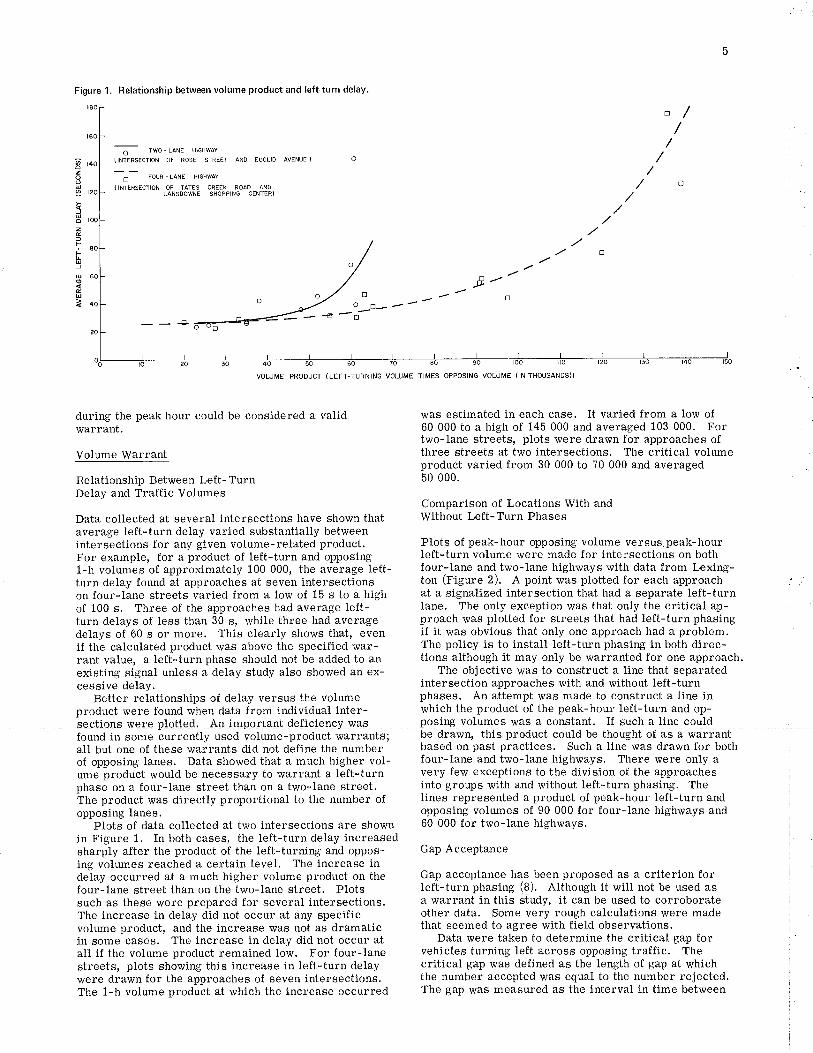
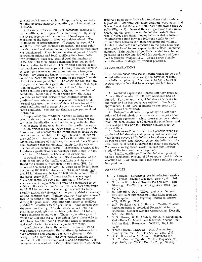
Figure 1. Relationship between volume product and left-turn delay.
ozoaUI
5UozElts
FUJ
uoÉu
^ TWO. LANE HIGHWAY
(INÍERSECTION OF ROSE STREÉT AND EUCLIO AVENUE )
-o- toun - Lare "'clwav
(INTERSECTION OF TATES CREEK ROAD ANDLÂNSDOWNE SHOPPING CENIER)
--4
during the peak hour could be considered a validwarrant,
Volume Warrant
Relationship Between Left- TurnDelay and Traffic Volumes
Data collected at several intersections have shown thataverage left-turn delay varied substantially betrveenintersections for anv given volume-related product.
40
E-/.vtr
70
VOLUME PROOUCT (LEFT-TURNING VOUJME TIMES OPPOSING VOLUME (INTHOUSANDS))
was estimated in each case, It varied from a low of60 000 to a high of 145 000 and averaged 103 000. Fortwo-lane streets, plots were drawn for approaches ofthree streets at two intersections. The critical volumeproduct varied from 30 000 to 70 000 and averaged50 000.
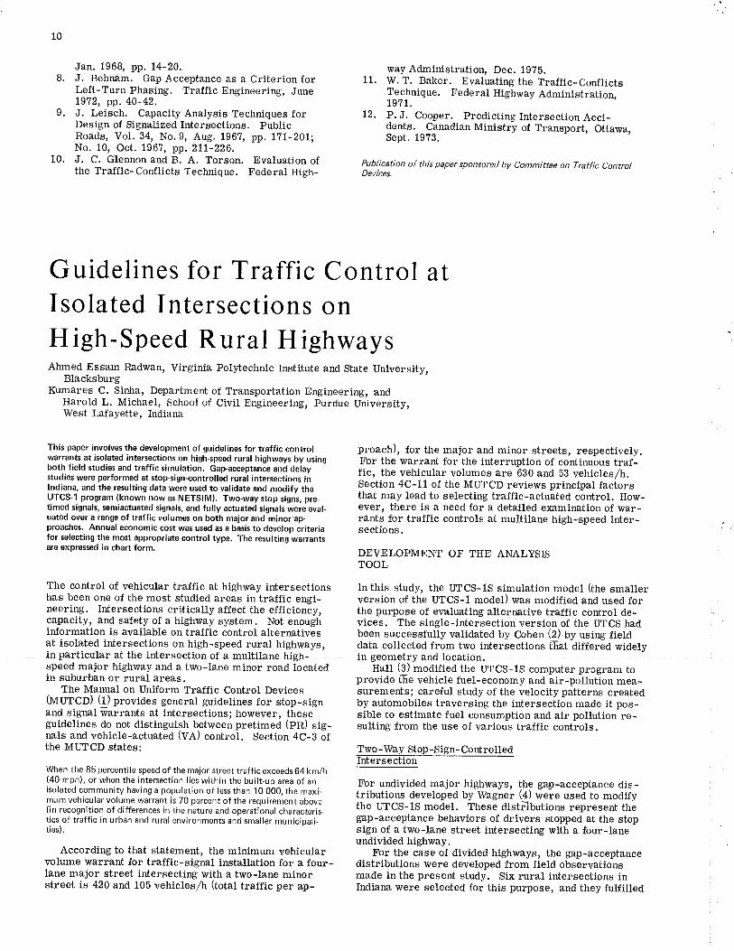
Comparison of Locations With andWithout Left- Turn Phases
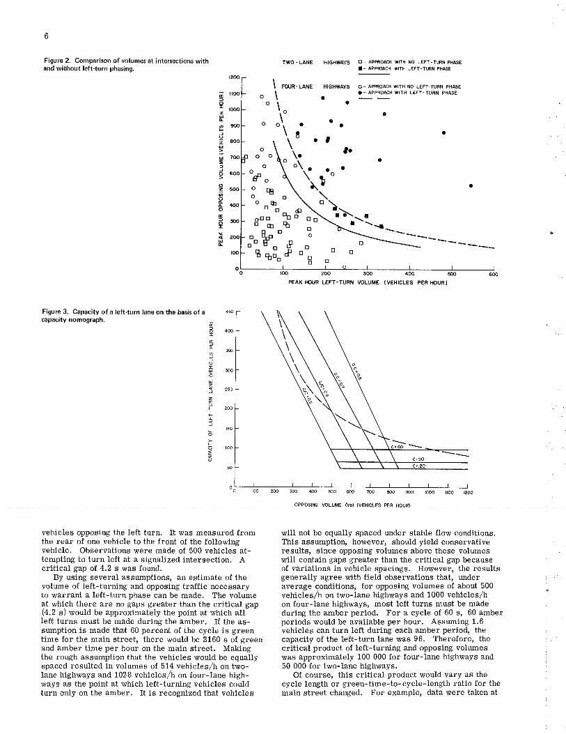
Plots of peak-hour opposing volume versus peak-hour
of 100 s. Three of the approaches had average left-turn delays of less than 30 s, while three had averagedelays of 60 s or more. This clearly shows that, evenif the calculated product was above the specified war-rant value, a left-turn phase should not be added to anexisting signal unless a delay study also showed an ex-cessive delay.
Better relationships of delay versus the volumeproduct were found when data from individual inter-èectio¡s¡uerqplotted-Anjmpo¡taut deücje4çylilLs pps:!¡g volumes wasa conqtaqt. It s,!SIL? q"elgqufoun6 in some currentlv used volume-oroduct warrants: be drawn, this product could be thought of as a warr
Iane. The only exception was that only the critical ap-proach was plotted for streets that had left-turn phasingif it was obvious that only one approach had a problem.The policy is to install left-turn phasing in both direc-tions although it may only be warranted for one approach.
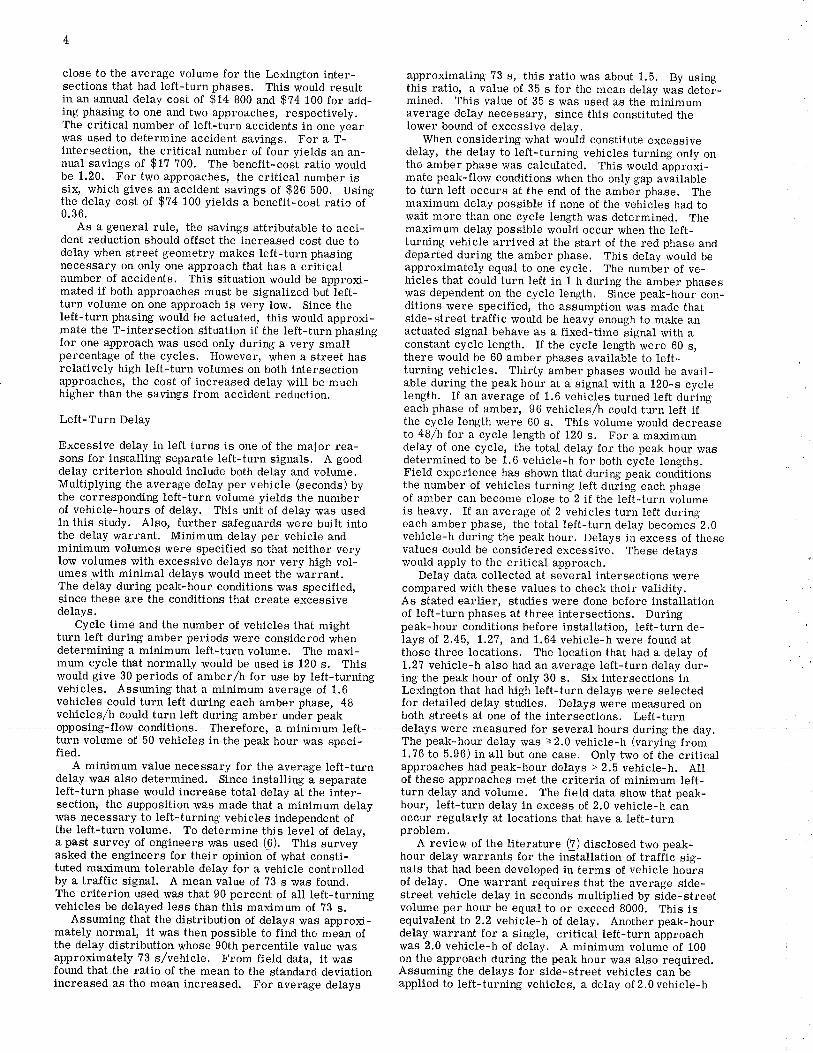
The objective was to construct a line that separatedintersection approaches with and without left-turnphases. An attempt was made to construct a line inwhich the product of the peak-hour left-turn and op-
found in some currently used volume-product warrants; as a warrantall but one of these warrants did not define the number based on past practices. Such a line was drawn for both
For example, for a product of left-turn and opposing left-t,urn volume were made for intersections on both1-h volumès of approimately 100 000, the average left- four-lane and. two-lane highways with data from Lexing-turn delay found ãt approaches at seven intersections ton (Figure 2). A point was plotted for each approachon four-lane streets varied from a low of 15 s to a high at a signalized intersection that had a separate left-turn
of opposing lanes. Data showed that a much higher vol- four-lane and two-lane highways' There were only aume product would be necessary to warrant a left-turn very few exceptions to the division of the approachesphasè on a four-lane street than on a two-lane street. into groups with and without left-turn phasing. Thethe product was directly proportional to the number of lines represented a product of peak-hour left-turn and
oppoãing lanes. opposing volumes of 90 000 for four-lane highways andplots of data collected at two intersections are shown 60 000 for two-lane highways.
in Figure 1, In both cases, the left-turn delay increasedsharply after the product of the left-turning and oppos- Gap Acceptanceing volumes reached a certain level, The increase indelay occurred at a much higher volume product on the Gap acceptance has.been proposed as a criterion forfour-lane street than on the trvo-lane street. plots left-turn phasing (8). Although it witt not be used as
such as these were prepared for several intersections . a warrant in this study, it can be used to corroborateThe increase in deláy did not occur at any specific other data. Some very rough calculations were made
volume product, and the increase was not as dramatic that seemed to agree with field observations.in some cases. The increase in delay did not occur at Data were taken to determine the critical gap forall if the volume product remained low. For four-lang vehicles turning left across opposing traffic. Thestreets, plots showing this increase in left-turn delay critical gap lvas defined as the length of gap at whichrvere dra-wn for the approaches of seven intersections. the number accepted r'vas equal to the number rejected.The 1-h volume product at which the increase occurred The gap was measured as the interval in time betrveen
6
Figure 2. Comparison of volumes at intersect¡ons withand without left-turn phasing.
TÌVO-LANE HtcHWAyS O- appRoacil WrfH flo LEFT-ILRN pHAsE
!- APPROACH WlH LEFl.flNN PHASE
cfIEúÀøEJ9¡u>-
U-lJo
IzØoÀÀoGforxuÀ
E3qmIGUd
350UJ9IUÐO¿Uz:! 2so
zElF 2ootsUJ
r tsooFõ rooÉo
il90
rooo
900
aoo
700
6()0
500
¿loo
I FOUR.LANE HIGHWAYS 9- APPROÁCII WITH t{O LEFI-IURN PBASE
I '-
APPROACH WITH LEFT-TURN PHASEo t a
--o
\o ',J . '. ';\; ¡ ,
oo o\ \.
roo 200 3m 400 aoo
PEAI( I.IOUR LEFT.TURN VOLUME (VEHICLES PER IIOURI
"r'. \"\, t'o '
too
o
Figure 3. Capac¡ty of a left-turn lane on the basis of acapacity nomograph.
vehicles opposing the left turn. It was measured fromthe rear of one vehicle to the front of the followingvehicle. Observations were made of 500 vehicles at-tempting to turn left at a signalized intersection. Acritical gap of. 4.2 s was found.
By using several assumptions, an estimate of thevolume of left-turning and opposing traffic necessaryto warrant a left-turn phase can be made, The volumeat which there are no gaps greater than the critical gap(4.2 s) would be approximately the point at which allleft turns must be made during the amber. If the as-sumption is made that 60 percent of the cycle is greentime for the main street, there would be 2160 s of greenand amber time per hour on the main street, Makingthe rough assumption that the vehicles would be equallyspaced resulted in volumes of 514 vehicles,/h on two-lane highways and 1028 vehicles/h on four-lane high-ways as the point at which left-turning vehicles couldturn only on the amber. It is recognized that vehicles
will not be equally spaced under stable flow conditions.This assumption, however, should yield conservativeresults, since opposing volumes above these volumeswill contain gaps greater than the critical gap becauseof variations in vehicle spacings. However, the resultsgenerally agree with field observations that, underaverage conditions, for opposing volumes of about 500vehicles/h on two-lane highways and 1000 vehicles/hon four-lane highways, most left turns must be madeduring the amber period. For a cycle of 60 s, 60 amberperiods would be available per hour. Assuming 1.6vehicles can turn left during each amber period, thecapacity of the left-turn lane was 96. Therefore, thecritical product of left-turning and opposing volumeswas approximately 100 000 for four-lane highways and50 000 for two-lane highways.
Of course, this critical product would vary as thecycle length or green-time-to-cycle-length ratio for themain street changed. For example, data were taken at
7
one intersection on a four-lane highway that had a cycle entirely on field data, there was a close agreement of
of 60 s and a green-time-to-cycle-tengttt ratio of about the results, A volume warrant based on aII sources of
0.?b for the niain street. For peak-hõur opposing vol- input was developed. The warrant required that the ad-
umes of srigtrtriãõie ttrãñ tvehicles did not have to turn during the amber. This when the product of left-turning and opposing volumes
was the result of more green time for the main street. during peak-hour conditions exceeds 100 000 on a four-By using the same assumptions as before, except that lane street or 50 000 on a two-lane street' A limitation?b percént of the cycle is assumed to be devoted to the is that the left-turn volume must be at least 50. This ismain street, a volúme of 1286 vehicles/h was the point based on the same reasoning as that for the minimum
at which lefi-turning vehicles could turn only on the am- volume requirement in the delay warrant. It is impor-ber. This would yiétA a critical product of iZ¡ OOO. tant to note that, even if the calculated product exceeds
the warrant, a left-turn phase should not be added to
Relationship Between Left-Turn Accidents an existing signal unless a study shows excessive left-and Traffic Volumes turn delaY'
By using the same Lexington data base' plots weredrawn of the highest number of left-turn accidents inone year for an approach versus the product of peak-hour left-turn volume and opposing volume, as well asjust the left-turn volume. The highest accident yearwas used so that a comparison could be made with thecritical accident number' The plots showed that therelationship was very poor in nearly all cases. Plotswere drawn for both two- and four-lane highways.'vVith one exception, the maximum coefficient of deter-mination (r2) was 0.2' The one exception was the plotof accidents versus the product of peak-hour left-turnand opposing volumes for four-lane streets; the r2
value for this plot was 0.5. Four accidents on an ap-proach in one year had previously been found to be
the critical number. This corresponded to a volumeproduct of approximately 80 000. A plot of left-turnäccidents veisus left-turn volume reiutted in an r2value of only 0.19. A value of four accidents relatedto a left-turn volume of 120. The inability to fit acurve to the points makes it hard to draw any validconclusions from the plots' However, the higher r'z
value for the plot that used the product of left-turningand opposing volumes indicates that this product was a
better estimator of left-turn accidents than was left-turn volume.
Capacity Analysis
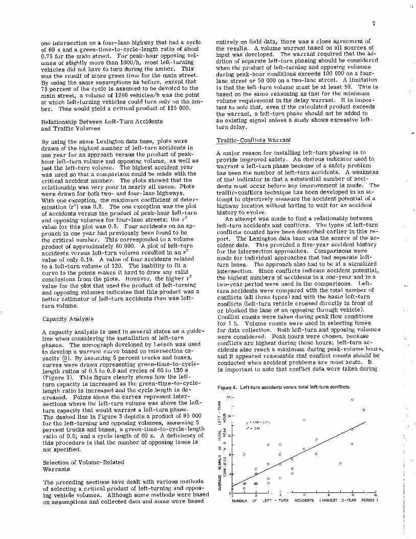
A capacity analysis is used in several states as a guide-line when considering the installation of left-turnphases. The nomograph developed by Leisch was usedto develop a warrant curve based on intersection ca-pacity (9). By assuming 5 percent trucks and buses,curves were drawn representing green-time-to-cycle-length ratios of 0.5 to 0.8 and eyeles ol 60 to 120 s(riàure 3). This figure clearly shows how the left-turn capacity is increased as the green-time-to-cycle-length ratio is increased and the cycle length is de-creased, Points above the curves represent inter-sections where the left-turn volume was above the left-turn capacity that would warrant a left-turn phase'The daÀhed line in Figure 3 depicts a product of 95 000for the teft-turning and opposing volumes, assuming 5
percent trucks and buses; a green-time-to-cyele-lengthiatio of 0.6; and a cycle length of 60 s. A deficiency ofthis procedure is that the number of opposing lanes isnot specified.
Selection of Volume-Related'rwarrants
The preceding sections have dealt with various methodsof selecting a critical product of left-turning and oppos-ing vehicle volumes. Although some methods were basedon assumptions and collected data and some were based
Traffic- Conflicts Warrant
A major reason for installing left-turn phasing is toprovide improved safety. An obvious indicator used towarrant a left-turn phase because of a safety problemhas been the number of left-turn accidents. A weaknessof that indicator is that a substantial number of acci-dents must occur before any improvement is made' Thetraffic-conflicts technique has been developed in an at-tempt to objectively measure the aecident potential of ahighway location without having to wait for an accidenthistory to evolve.
An attempt was made to find a relationship between.Ieft-turn accidents and conflicts. The types of left-turnconflicts counted have been described earlier in this re-port. The Lexington data base was the source of the ac-cident data. This provided a five-year accident historyfor the intersection approaches. Comparisons weremade for individual approaches that had separate left-turn lanes. The approach also had to be at a signalizedintersection. Since conflicts indicate accident potential,the highest numbers of accidents in a one-year and in atwo-year period were used in the comparisons. Left-turn accidents were compared with the total number ofconflicts (all three types) and with the basic left-turnconflicts (left-turn vehicle crossed directly in front ofor blocked the lane of an opposing through vehicle).Conflict counts were taken during peak flow conditionsfor t h. Volume counts were used in selecting timesfor data collection. Both left-turn and opposing volumeswere considered. Peak hours were chosen, becauseconflicts are highest during these hours; left-turn ac-cidents also reach a maximum during peak-volume houts,and it appeared reasonable that conflict counts should beconducted when accident problems are most acute. Itrcj4ppl!4nt t! 49!9 tÞt qo"fqc! satq 1grltqeq lgltns
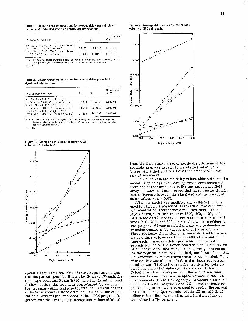
Figure 4. Left-turn accidents versus total left-turn conflicts.
zÉlFtetsÞuoUTJ
J4<U5dh
ozÉ
=s¿fJZLzoUOoÊüI
y=1.58+l.17x
12 - 0.61
NUMBER OF LEFT - TURN ACCIDENTS ( HIGHEST z.YEAR PERIOD )
I
Table 2. Relationship between left-turn accidents and left-turn conflicts.
Linear Critical
U".rror" fã
Nmber of total conflictsversus
Highest one-yearperiod of accidents
Highest two-yearpe¡iod of accidents
Nmb€r of basic conflictsversus
Highest one-yearperiod of accidents
Highest two-yearperiod of accldents
'Y = number of conflicts; X = number of accidents.b Probab¡l¡ty level = 95 percent.
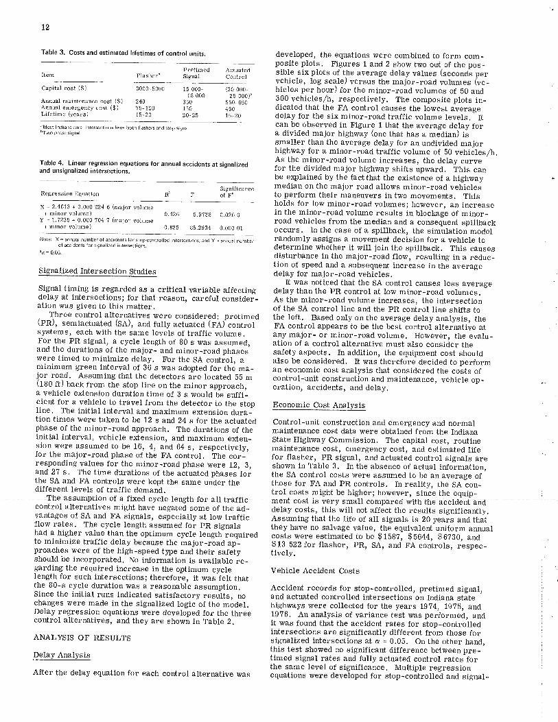
Figure 5. Total left-turn conflicts in peak hour versus product of peak-hour left-turn volume and opposing volume.
Y = 1.26 + 1.87X 0.50 8.?
Y = 1.58 + 1.1?X 0.61 8.6
Y = 1.42 + 1.13X 0.39 5.9
Y = 1.?0 + 0.69X 0.45 5.8
5.4
4.8
4.7
3.9
tr
t6
t5
9
I
o //
//
/t^'ooa xo'lt'= O 44
GãIE
H-ol-9Jltt(Jz,5FI
EJt-oF
^ IWO - LANE
-n- FOUR - LANE
o
Ì
È,
u-f-
E)
ooy.1.97 x lo-l ro?3
¡!' 0.76
5,O0O 0ooo sqooo þqooo
PRODIJCT OF PEAK HOI.R LEFT-Ttnil \þLUffi AIf) oPFæII{G \Ioum
I
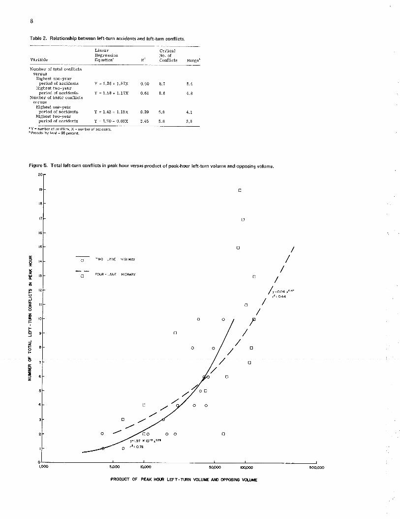
several peak hours at each of 82 approaches, so that a Separate plots were drawn for four-lane and two-lane
reliable average number of conflicìs per hour could be highways. Both total and basic conflicts were used, and
obtained. it was found that the use of total conflicts gave better re-
turn conflicts; see Figure 4 for an example. By using tried,,and the power curve yielded the best-fit line.Iinear regresÁion andlhe method of least squares, The r' values for these figures indicate that a better
equationiof the best-fit lines were determined. ifte relationship exists between left-turn conflicts and
coefficients of determination (r') ranged between 0.3g volume than bet',veen left-turn accidents and volume'
and 0.61. For both conflict categoriãs, the best rela- A total of nine left-turn conflicts in the peak hour was
tionship was found when the two--year accident maximum previously found to correspond to the critical accident
was considered, Also, better reiationships were found number. This number of conflicts related to volume
between accidents and total conflicts than basic left- products of 65 000 and 100 000 for two-lane and four-turn conflicts; however, data showed the number of lane highways' respectively' These agree closelybasic conflicti to be more consistent from one period with the other findings for critical products.
of observation to the next. The critical number of left-turn accidents for one approach was previously found tobe four for a one-year period and six for a two-yearperiod. By using the linear regression equations, thenumber of conflicts corresponding to the critical numberof accidents was predicted. The equations for one- andtwo-year accident data gave similar results. The equa-tions predicted that about nine total conflicts or sixbasic conflicts corresponded to the critical number ofaccidents. Since the 12 values were low, the range(confidence interval) within which conflicts could bepredicted was determined' A probability level of 95percent was used. A range of about Ì5 was found fortotal conflicts, and a range of about +4 was found forbasic conflicts, The various findings are summarizedin Table 2.
Simply using the predicted number of conflicts re-lated to the critical accident number as a warrant forleft-turn signalization would not be very reliable; thisis so because of the uncertainty of the prediction equa-tion, as evidenced by the large range in values possible.A warrant that considered the confidence interval rvouldbe much more reliable. The upper bound of values in
' the confidence interval was used as the conflict warrant.Given that number of conflicts, there rvould be a 95 per-cent certainty that the potential exists for the criticalnumber of accidents to occur. Therefore, a warrant forIeft-turn signalization was developed that listed 14 totalconflicts or 10 basic conflicts as its criterion.
A recent report included a critical evaluation of thestate of the art of the traffic-conflicts technique and
. listed the results of work done in this area (10). Interms of accidents per conflict, there were 20 left-turnaccidents,/lO0 000 lãft-turn conflicts in one study (11)
and 15 left-turn accidents,/100 000 left-turn conflicts inthe other study (12). If those results are averaged
critical, the critical number of left-turn conflicts wouldbe 22 851 in one year. Assuming the conflicts to be
equally distributed throughout the year yielded an averageof 62.6 conflicts/day. Volume data for Lexington showedthat 14 percent of the daily left-turn volume occurredduring the peak hour. Applying this factor to conflictsyielded ?.0 conflicts in the peak hour. This agreed withthe previous finding: 6 basic left-turn conflicts in apeak hour would give an accident potential of 4 left-iurn accidents in one year. Thosè two studies gave r'values of 0.38 and 0.1i. The values for rz from 0.39 to0,61 found for the linear regression lines of accidentsand conflicts in this study compared favorably.
Conflicts are inherently related to volume. Plotswere drawn to determine the relationship between left-turn conflicts and volumes for data collected in thisstudy. Peak-hour conflicts were plotted against theproduct of left-turn volume and opposing volume. Vol-umes were counted while the conflict data were collected'
RECOMMENDATIONS
It is recommended that the following warrants be usedas guidelines when considering the addition of sepa-rate left-turn phasing. The warrants apply to inter-section approaches that have a separate left-turnlane.
1. Accident experÍence-Install left-turn phasingif the critical number of left-turn accidents has oc-curred, For one approach, 4 left-turn accidents inone year or 6 in two years are critical. For bothapproaches, 6 left-turn accidents in one year or 10
in two years are critical.2. Delay-Install left-turn phasing if a left-turn
delay of 2.0 vehicle-h or more occurs in a peak houron a critical approach, AIso, there must be a mini-mum left-turn volume of 50 during the peak hour, andthe average delay per left-turning vehicle must beat least 35 s.
3. Volumes-Consider left-turn phasing when theproduct of left-turning and opposing volumes duringpeak hours exceeds 100 000 on a four-lane street or50 000 on a two-lane street. Also, the left-turn vol-ume must be at least 50 during the pçak-hour period.Volumes meeting these levels indicate that furtherstudy of the intersection is required.
4. Traffic conflicts-Consider left-turn phasingwhen a consistent average of 14 or more total left-turnconflicts or 10 or more basic left-turn conflicts oceursin a peak hour.
REFERENCES
1. T. Yamane. Statistics: An Introductory Analy-sis, 2nd ed. Harper and Row, New York, 196?.
Phasing. Traffic Engineering, June 1969, pp'50- 53.H. Sofokidis, D. C. Tilles, and D. R' Geiger.E valuation of Inte r section- Delay Meas urem entTechniques. HRB, Highway Research Record453, L973, pp. 28-39.S. R. Perkins and S. J. Harris. Traffic ConflictCharacteristics: Accident Potential at Inter-sections. General Motors Corporation, Detroit'MI, Dec. 196?,V. G. Stover, W.G. Adkins, and J. C. Goodknight.Guidelines for Medial and Marginal Access Con-trol on Major Roadways. NCHRP, Rept. 93'19?0.Traffic Signal Warrants. KLD Associates,Huntington, NY, KLD TR No. 17, Nov. 19?3.P. C. Box and W. A. Alroth' Warrants forTraffic Control Signals. Traffic Engineering'Nov. 196?, pp. 32-41; Dec. 1967, pp' 22-29;
(1?-b accidedÊ11o! 0!q confliets) and if 4 Iaccidents on an approach in a year is considered to be 2. f. furnett. IñtêÍsectiõn Dêlafãnd Left=T-urn
3.
4.
5.
6.
1.
10
Jan. 1968, pp. 14-20. way Administration, Dec. 19?b.8. J. Behnam' Gap Acceptance as a criterion for 11. w. T. Baker. Evaluating the Tra-ffic-conflictsLeft-Turn Phasing. Traffic Engineering, June Technique. Federal Higiway Administration,1912. gp. 40-42. tg,t!. -
9. J. LeÍsch. Capacity Analysis Techniques forDesign of Signalized Intersections. PublicRoads, Vol. 34, No.9, Aug" 1967, pp. L7l-20t;No. 10, Oct. 196?, pp.2tL-226,
10. J. C. Glennon and B. A. Torson. Evaluation ofthe Traffic-Conflicts Technique. Federal High-
L2, P. J. Cooper. Predicting Intersection Acci-dents. Canadian Ministry of Transport, Ottawa,Sept. 19?3.
Publication of this paper sponsored by Committee on Traffic ControtDevices.
proach), for the major and minor streets, respectively.For the warrant for the interruption of continuous traf-fic, the vehicular volumes are 630 and 53 vehicles/h,Section 4C-11 of the Mti"TCD reviews principal factorsthat may lead to selecting traffic-actuated control. How-ever, there is a need for a detailed e¡ra.mination of war-rants for traffic controls at multilane high-speed inter-sections.
DEVELOPME}TT OF THE ANALYS$TOOL
In this study, the IIICS-1S simulation model (the smallerversion of the üICS-1 model) was modiJied and used forthe purpose of evaluating alternative traffic control de-vices, The single-intersection version of the IJTCS hadbeen successfully validated by Cohen (2) by using fielAdata collected from two intersections tlat differed widelyin geometry and location.
HaU (3) modified the IITCS-15 computer program toprovide t-ñe vehicle fuel-economy and ãir-pollution mea-surements; careful study of the velocity patterns createdby automobiles traversing the intersection made it pos-sible to estimate fuel consumption and air pollution re-sulting from the use of various traffic controls.
For undivided major highways, the gap-acceptance dis-tributions developed by Wagner (4) were used to modifythe IJTCS-IS model. These distr-ibutions represent thegap-acceptance behaviors of drivers stopped at the stopsign of a two-lane street intersecting with a four-laneundivided highway.
For the case of divided highways, the gap-acceptancedistributions were developed from field observationsmade in the present study. Six rural intersections inIndiana were selected for this purpose, and they futJilled
Guidelines for Traffic Control atIsolated Intersections onHigh-Speed Rural HighwaysAhmed Essam Radwan, virginia Polytechnic Institute and state university,
BlacksburgKumares C. Sinha, Department of Transportation Engineering, and
Harold L. Michael, School of Civil Engineering, Purdue University,West Lafayette, Indiana
This paper involves the development of guidelines for traffic controlwarrants at ¡solated intersections on high-speed rural highways by usingboth field studies and traffic simulation. Gap-acceptance and delaystudies were performed at stop-sign-controlled rural ¡ntersect¡ons inlndiana, and the result¡ng data were used to val¡date and mod¡fy theUTCS-I program (known now as NETSIM). Two-way stop signs, pre-timed signals, semiactuated signals, and fully actuated signals were eval-uated over a range of traffic volumes on both major and minor ap-proaches. Annual economic cost was used as a basis to develop criteriafor selecting the most appropr¡ate control type. The resulting warrantsare expressed in chart form.
The control of vehicular traffic at highïray intersectionshas been one of the most studied areas in traffic engi-neering. Intersections critically affect the efficiency,capacity, and safety of a highway system. Not enoughinformation is available on traffic control alternativesat isolated intersections on high-speed rural highways,jn+adicular at the-intersection oÈa multilane high-speed major highway and a two-lane minor road locatedin suburban or rural areas.
The Manual on Uniform Traffic Control Devices(Utff CO) (1) provides general guidelines for stop-signand signal warrants at intersections; however, theseguidelines do not distinguish between pretimed (pn) sig-nals and vehicle-actuated (VA) control. Section 4C-3 ofthe MIIICD states:
When the 85 percentile speed of the major street traffic exceeds 64 km/h(40 mph), or when the intersection lies within the bu¡lt-up area of anisolated community having a population of less than 10 000, the maxi-mum vehicular volume warrant is 70 percent of the requirement above(in recognition of differences in the nature and operational characteris-tics of traffic in urban and rural environments and smaller municipali-ties).
According to that statement, the minimum vehicularvolume warrant for traffic-signal installation for a four-lane major street intersecting with a two-lane minorstreet is 420 and 105 vehicles/h (total traffic per ap-
Two -Way Stop -Sign- ControlledIntersection
11
Table 1. Linear regression equations for averaç delay per vehicle ondivided and undivided stop-sign-controlled intersections.
Figure 2. Averaç delay values for minor'roadvolume of 300 vehicles/h.
negression Equation
Y = 2.1368 + 0.001 841 (major volume)+ 0,002 113 (minor volume) 0.71'l'l
z = 7.5543 + 0.001 054 (major volume)+ 0.010 46 (minor volume) 0.8379 100.8126 0.000 01
Note: Y = Naperian logarithm (âverage delay per vehicle on und¡vided major highwây); and Z= Naperian logarìthm {average delay per veh¡cle on divided mâjor highway).
"a = 0.05.
Table 2. Linear regression equat¡ons for average delay per vehicle ats¡gnalized intersections.
0.000 01
0.oJ.J
dØ
Regression EquâtionSignificance ! s,ooofF å
X = 2.6564 + 0.000 386 6 (ma.jor
volume)+ 0.001 861 (minor volume)Y = 1.1239 + 0.002 862 (major
volume) + 0.003 43? (minor volume)Z = l.B7l4 + 0.000 ?24 9 (major
volume) + 0.003 1?5 (minor voÌume)
0.?453 48.2861 0.000 01
0.8?84 0.000 01
0.?365 46.1393 0.000 01
oooãqq
(9oJ
LØ
oõooÞo
Note: X = Naper¡an logarithm (average delay for pretimed signalsl; Y = Naperian logar¡thm(average delay lor semiâctuated control); and z = Naper¡an logôrithm {average delayfor fully actuated control).
"a = 0.05.
Figure 1. Averaç delay values for m¡nor-roadvolume of 50 vehiclesih.
specific requirements. One of these requirements wasthat the posted speed limit must be Sg km/h (55 mph) forthe major road and 64km/h (40 mptr) for the minor road.A slow-motion film technique was adapted for securingthe necessary data, and gä.p-acceptanee distributions fordifferent maneuvers were obtained. By using the distri-bution of driver type embedded in the IIICS program to-gether with the average gap-acceptance values obtained
1400 vehicles/h), and three levels for minor traffic vol-ümes (lOOJ0O, and S00 vehicles/h)r ¡pere eonsidered-
from the field study, a set of decile distributions of ac-ceptable gaps ì,vas developed for various maneuvers.These decile distributions were then embedded in thesimulation model.
In order to validate the delay values obtained from themodel, stop delays and move-up times were measuredfrom one of the films used in the gap-acceptance fieldstudy. Statistical tests showed that there r,vas no signifi-cant difference between the simulated and the observeddelay values at q = 0.05.
After the model ï¡as modified and validated, it wasused to perform a series of large-scale, two-way stop-sÍgn-controlled intersection simulation runs. Fourlevels of major traffic volumes (500, 800, 1100, and
The purpose of these simulation runs v/as to develop re-gression equations for purposes of delay prediction.Three replicate simulation runs were obtained for everymajor-minor volume combination (+OO of simulationtime each). Average delay per vehicle measured inseconds for major and minor roads was chosen to be thedelay measure for this study. Homogeneity of variancesfor the replicated data was checked, and it was found thatthe Naperian logarithm transformation was needed. Testof normality \üas also checked, and a linear regressionequation was fitted to the transformed data for both di-vided and undivided highways, as shovrn in Table 1.Velocity profiles developed from the simulation runswere used as an input to an adapted version of the U.S.Environmental Protection Agency' s Automobile ExhaustEmission Modal Analysis Model (5). Simitar linear re-gression equations urere developei[to predict the amountõf fuel cons-umed þer vehicte) within 122 m (400 ft) ofeither side of the intersection, as a function of maiorand minor traffic volumes.
3.6
L2
Table 3. Costs and estimated lifetimes of control units.raore r. uosIs anq esümared ttïettmes ot control un¡ts- develOped, the equatiOns Were Combined tO form COm_
",""r,*. ^_*". posite plots, Figures 1 and 2 show two out.of the pos-
rt"^ rr""r,"r" stgr sible six plots of the average delay values (seconds per
Capital cost ,*,
Annual maintenance cost (g) z4o ,# ooo
,åt-333f 300 veñicles/h, respectively. The composite plots in-Annual emergency cost (g) ?b-100 1b0 4b0 dicated that the FA control causes the lowest averageLifetime (yea¡s) 1b-Zo 20-25 1b-zo delay for the six minor_road traffiC volume levels. ItaMostlnCjiânarural'"-canbeobservedinFigure1thattheaveragede.1ayforbrwophasesisnar. a divided major highway (one that has a median) is
smaller than the average delay for an undivided majorhighway for a minor-road traffic volume of b0 vehicles/h.
Table 4. Linear regression equations for annual accidents at signalized As the minor-road volume increases, the delay curveand unsignatized intersecrions.
sr rrvrrorr'Eu for the divided major highway shifts upward. This canbe e:çlained by the fact that the existence of a highway t
Iïïïïry" ;:ii?ä:å,if"i"#å::î:å"1"-åiil:i;å"å$J:1ï.iiJx=2.46l3*o,ooholdsforlowminor-roadvolumes;however,anincrease
+ minor votume) 0.426 b.b?3g 0.026 0 in the minor-road volume results in blockage of minor-y = 1.?235 + 0.000 ?04 7 (ma.ior volume road vehicles from the median and a consequent spillback+ mino¡ volume) 0 825 85 2934 0.000 01 occurs. In the case of a spillback, the simulation modelrandomlyassignsamovementdecisionforavehic1etooracc¡rJentsrorsisnalizedíntersections determine whether it witl join the spillback. This causes¡c=0'0s disturbance in the major-ioad flow, resulting in a reduc-
sisnarized rntersection srudies :'Jå;ijii3j3::ff;iJri:e¡t.increase in the averag
It was noticed that the SA control causes less averageSignal timing is regarded as a critical variable affecting delay than the pR control at low minor-road volumes.delay at intersections; for that reason, careful considei- As the minor-road volume increases, the intersectionation was given to this matter. of the SA control line and the pR control line shifts toThree control alternatives \¡/ere considered: .pretimed the left. Based only on the average delay analysis, the(PR), semiactuated (sA), and rutty actuàié¿ (i;alï*i"åi- FA control appears to be the best controt alternative atsystems, each with the same levels of traffic volume, any major- oï minor-road volume. However, the evalu-For the PR signal, a cycle length of B0 s was assumed, ation of a control alternative must also consider theand the durations of the major- and minor-road phases safety aspects. In addition, the equipment cost shouldwere timed to minimize delay. For the SA control, a also be considered. It was therefore decideo to performminimum green interval of 36 s was adopted for thé ma- an economic cost analysis that considered the costs ofjor road. Assuming that the detectors are located bb m control_unit construction and maintenance, vehicle op_(fgO tt) back from the stop line on the minor approach, eration, accidents, and delay.a vehicle extension duration time of B s would be suffi_cient for a vehicle to travel from the detector to the stop Economic Cost Analysisline. The initial interval and maximum extension dura_tion times were taken to be t2 s and 24 s for the actuated Control-unit construction and emergency and normalphase of the minor-road approach. The durations of the maintenance cost data were obtained from the Indianainitial interval, vehicle extension, and maximum exten- state Highway Commission. The capital cost, routinesion were assumed to be 16, 4, and 64 s, respectively, maintenãnce cost, emergency cost, and estimated lifefor the major-road phase of the FA control. The cor-' for flasher, PR signal, and actuated control signals are '..responding values for the minor-road phase were 12, 3, shown in fâ¡te S. In the absence of actual information,and 27 s' The time durations of the actuated phases-for the SA control costs were assumed to be an average ofthe SA and FA controts were kept the same under the those for FA and pR controls. In reality, the SA con-different levels of traffic demand. trol costs might be higher; however, since trre equip-
Annual emergency cost ($)Lifetime (yea¡s)
75- 10015-20
'Most lndiâna rural intersections have both flashers ând stop signs_bTwo phase siqnal.
Table 4, Linear regression equations for annual accidents at signal¡zedand unsignalized intersections.
" SignificanceR' F ofF'
X = 2.4613 + 0,000 224 6 (major volume+ minor volume) 0.426 b.b?39 0.026 0
Y = 1.7235 + 0.000 ?04 ? (ma.ior volume+ minor volume) 0.825
4he assumpíion of a fixed eyele length for all Èraffic ment cosf isvrry smill cémparediith fhe acclilenfãñfcontrol alternatives might have negated some of the ad_ delay costs, this will not affect the results significanily.vantages of SA and FA signals, especially at low traffic Assúming tÍrat the life of all signals is 20 years and thatflow rates. The cycle length assumed for pR signals they havã no salvage value, the equivalent uniform annualhad a higher value than the optimum cycle length required costs were estimaied to i": Eiáeil-çáo¿¿, $oz¡0, "n¿to minimize traffic delay because the major_road ap_ $13 b22 i"" n""tô",-pR, SA, and FA controls, respec_proaches were of the high-speed t5zpe and their safety tively.
should be incorporated. No information is available re_garding the required increase in the optimum cycle Vehicle Accident Costslength for such intersections; therefore, it was felt thatthe 80-s cycle duration was a reasonable assumption, Accident records for stop-controlled, pretimed signal,Since the initial runs indicated satisfactory results, no and actuated controlled intersections on Indiana statechanges were made in the signalized logic of the model. highways were collected for the years 1g74, 19?5, andDelay regression equations were developed for the three tg76, ¿n analysis of variance test was performed, andcontrol alternatives, and they are shown in Table 2. it was found thát the accident rates for Jtop_controlled
ANALysrs oF REsuLr, :T!ï:;1å"iååiå:li#:'ï'yl åTri;:.åi',ïåtH:îå";,perav Analvsis titr":":l-"iÎäî#JJ.'T""i,i*åTf:ä"å"ï.fffHå":ïAfrer the deray equarion for each control auernative was 3äffiå:T#:i:i:iäfjå,Tï;,#:ji"l,tåí,""*0"åiåt3i*"r-
ized intersections to be used in estimating an annualnumber of accidents, as shown in Table 4.
One survey of particular relevance to this research
13
this study. By using the severity fractions, the directcosts, and the indirect-cost value, the weighted aver-age cost per accident was found to be $1595.
was performed by HeJaI and Mrcnael \þ/ to evaruate tnedirect cost per rural accident in Indiaña. By updatingthe accident cost values to 1978 prices with the aid ofthe appropriate consumer price indices, the figureswere estimated to be $25 954, $59?1, and $845 forfatal, personal injury, and property-damage-only acci-dents, respectively.
In order to determine the average cost of an accident,the study conducted by Abramson (?) was used; in thisstudy, the results of statewide accident in:formation fromIllinois, Massachusetts, Utah, and New Mexico wereused. By assuming that the results of this study are ap-plicable to the state of Indiana, the fractions of fatal,personal injury, and property-damage-only accidentswere estimated to be 0.0041, 0.0826, and 0.9133, re-spectively.
A recent study by Wuerdemann (B) proviOed nationalindirect costs of motor vehicle acciîents. An averageindirect cost value of $160/accident was adopted from
Automobile Operating Cost
Knowing the quantity of gasoline consumed in driving avehicle through an intersection under the four types ofcontrol alternatives, as simulated by the UTCS-ISmodel, permitted gasoline cost calculations. It wasassumed that the average cost of gasoline was 17 cents/L(64 cents/gal) in 19?8. Federal and state gasoline taxes,which accounted for 3.5 cents/L (13 cents,/gal) of thisprice, are returned to the road user through maintenancebenefits. Hence, the actual gasoline operating cost wasassumed to be 13.5 cents/L (51 cents/gal).
Winfrey (9) estimated the other automobile operatingexpenses (tiies, oil, maintenance, and depreciatioil onthe basis of empirical data. By updating these prices to1978 dollar values, it was found that the other operatingcosts were 1.980 and 1.806 cents/vehicle for major- andminor-road signalized approaches, respectively. As for
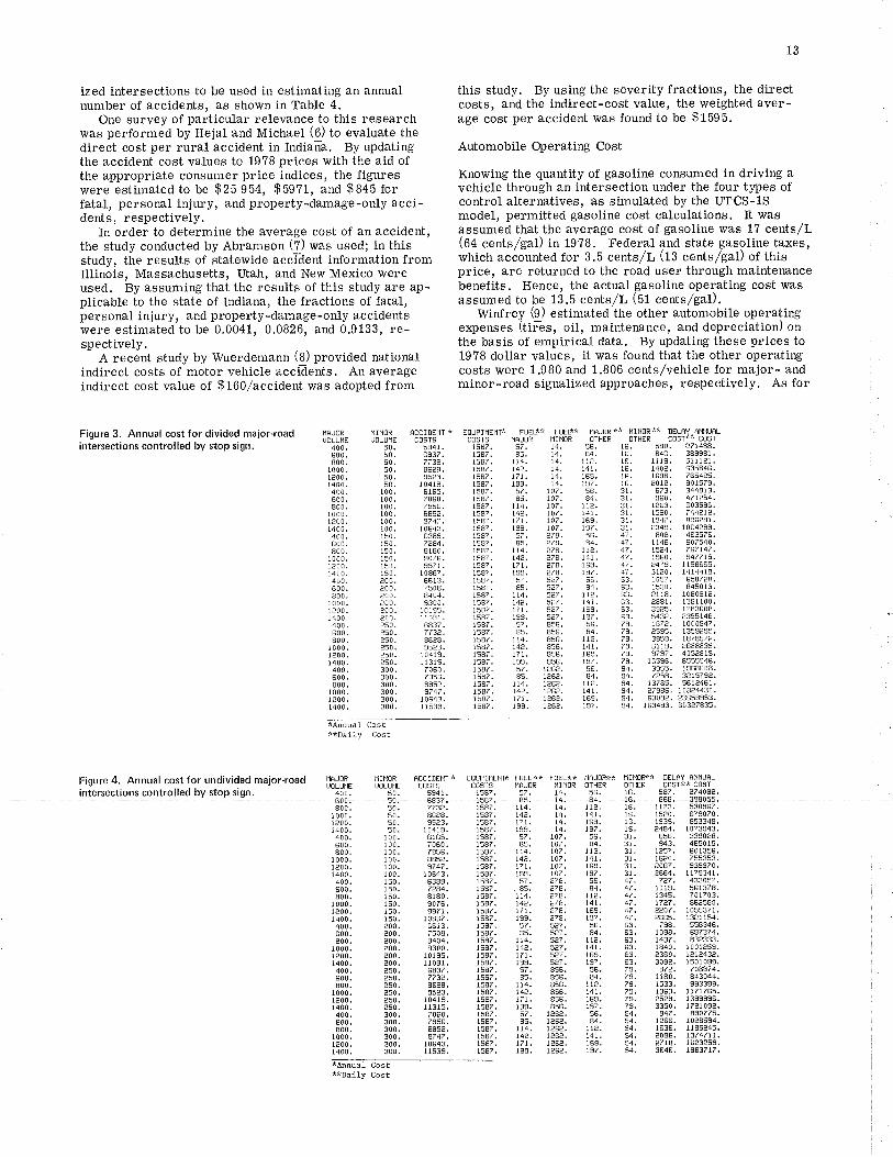
Figure 3. Annual cost for divided major-road¡ntersect¡ons controlled by stop sign.
ÊccIDEN'I * E0UPItlENlk FU€L** FUEü|*COSTS COSTS HâJOR I1INOR
594I. 1587. 57, 14.6837. 1587. 85, !4.7732, 1587. ll4, 14.8628. 1587. 142. 14.9523. LsA?. l7r. 14.
r04lg. t5a7. lss. 14,6165. 1587. 5?. L07,7060. 1587. 85. 107.79s6. 1587, ll4. 107.88se. 1587, 142. 107.974? . 15a7. l7L 107.
10643. 1587. 199. 107.6389. 1587. 57. 274.7?A4. t5A7. 85. ??4.8180. 1587. ll4. e7A,9076. 1587. 142. ?74.997r. 1587. l7l. ?74.
10867. r5A7. tgs. 278.6613. 1587. 57. 527.7508. LSA7. 85. s27.a404. rsaz. il4. 5¿7.9300. 1587. r4?. 5?7.
r 0 rg5. 15a7. t? |, 5?7 .I I 09r. 1587. r93, 5¿7 .6A37, 1587, 57, 856.773?. 1587. 85, 85S.8628. 1587. ll4. 856.9523. .1587. l4?. 856,
10413. 1587. l7l. 856.I 1315, 1587. r99. 856.7060. 1587, 57. 1262.7956. 1587, 8s. 126e,885e. 1587, ll4, 1?6?.3747. 1587. L4e. 1¿6¿.
10643, 1587. 171. 126e.11539. 1587. 199, I26e,
ffAJOR** ÍINOR** DELÂY ANNUÊTorHER orHER cosr** cosr
56. 16, 580. ?714A8.84. 16, 846, 389981.
It¿, 16. lll9, 5lll2l.l4t. 16. 1402, 635846.169, 16. 1698. 76s4P5,rs7. 16. 201?. 901579.56, 31. 673, 344913.84. 31. 960. 471?54.
1r2. 31. 1263. 603596,141. 31. 1530. 744e1?.169. 3t, 134?. 896e81.197. 3l, 4349. 1064299.56. 47, 808. 462576.a4. 4?. 1146, 607540.
1 le. 47 . 1524. 76? 14? .141. 47. 1360. 3477t3.169. 47. 2473. 1158665.t97, 47 . 31e0. 1414419.56. 63. 1057. 650728..84. 63. 1530. 845013.
112. 63. 2118. 1080912.141. 63. 2881. 1381100,169. 63. 3925. 1783608.r97. 63. 5432, 4355146.56. 73, 1672, 1000347.84. ?3, e595. 1359255.
lle. ?3. 3359. 1878972.141. 7s. 6119, 2688839.169. 79. 9797. 4052819.rs7. 7s. 16596. 6555946,s6. 34, 3955. 1988608.a4. 94. 725A. 3?15732,
112. 94. 13765. 561¿461.14r. s4. ?7986. 10844430.r6s. 94, 63032, 23659953,197. 34. t63493. 603¿7835.
I1AJOR ilINORUOLUI1E UOLUT1E
400. 50.600. 50,a00. 50.
1000. 50.1200. 50,1400, 50.400. 100.600. 100.800. 100.
1000, 100.1200. 100.1400. ¡00,400, t50.600, 150,800. 150.
1000. 150.1200. 150.1400, r50.400, e00.600, 200.800. 200.
1000. ¿00.1200. ¿00,1400. 200,400. e50.600. e50.a00. 250.
1000. e50,1200. 250,1400, 250.400, 300.600. 300.800. 300.
1000, 300.1200. 300.t400. 300.
*Annuêl Cost**Daily cost
Fisure4. Annualcostforundividedmajor-road i3J3[. üåi!i. .33ëlE"'. '33!+!.*. [X5bå. 'Hihåå |îi!f. HilPF-. !E!îï.^iä!î'
intersections controlled by stop sign. 400, s0. sgqr. lssz, s7. 14. s6, 16. s87. 2?40a¿.0-û-683?. 1587- €5. 14- €4-15. €6e. J38055'
800. 50. 7ße. 1587, 1r4. 14. 1te' 16. 1173. 530367.1000, 50. 86e8. 158?. L4?, 14. 141. 16, 1520. Ê79070.t200. 50. 95e3. 1587. L7l, 14. 169. 16. 1939. 85334S.1400. 50. 10419. 1587. 199. 14. 197. 16' 24A4. 10?3343.4oo. 100. 6165. 1587. 5? ' lO7. 56. 31. 956. 339028'600. 100. 7060. 1587. 85. 107 ' 84. 31. 943. 465015.800. 100. 7956. 1587. Il4. 107. 1r2. 31. 1257- 601356.
lo0o. lo0. 885e. 1587. l4?, lO7, t4l. 31. 1Se0. 755353.leoo, 100. 9747. 1587. 171, 107, 169. 31. ?067. S3S370.1400, 100. 10643. 1587, 199. 107. 197' 31. ¿664' 117334¡.400. r5o. 6389. ¡587. 57. ?7A, 56' 47. 727 ' 433057.600. I5o. 72A4, 1587. . 85, A7A, A4' 4?. 1019. 581378.800. l5o. 8180. 158?. 114. ?78, 112, 47. 1345. 701703'
tooo. 150. 3076. 1587. l4?. "7A,
141. 47. !??7. 862580.leoo, 150. 997t. 1587, 1?1' ?7A. 16S. 47. e407. 1059371.1400. 150, 10867. 1587. 193. 27A. 197. 47. e865. 1321154.400. aoo. 6s!3, 1587. 57, 5?7. 56' 63' 798. 556346'600, eoo. 7508. 1587. 85. 5?7. 84. 63. 1098. 847374.800. eoo. 8404. 1587. lt4. 527. 1l¿. 63. 1437. 832333.
1000. eoo, 9300. 1587' l4a. S?7. L4l. 63. 1840' t001259.te00. eoo. 10195. 1587. l7L, 5?7, 169' 63. e360. lale43e.1400. 2oo. llo91. 1587. 199. 527. 137. 63. 309e' 150.10s9.4oo, eso. 6837. 1587. 57 ' 856. 56' 79. A72. 704474,600. e50, ?73?. 1587. 85. 856. A4. 73. ll80' 443044.8oo. eso. 8628. 1587. tl4. 856. li.e' 79. 1533. 993399'
1ooo. 250. 35e3. 1587. 142. 856. 141' 79. 1963. 1171765.1¿OO. 250. 10419. 1587. l7l. 856. 159' 79. 2529. 1399396.1400. eso. ll3t5. t587. t99. 856. 197' 79' 3350. 17ar0S2'4oo. 300. 7060, 158?. 57. 1262. 56' 34. 947. 830775.600. 3oo. 795t' 1587. 85. 1262. 84. 34. 1466. 1028594.8oo. 3oo, 885¿, 1587. 114. 126e. lla. 94' 1536. 1185245.
1000, 300. 9?47. 1587. L4?, 1262. 1,41. 94. 2096. 1374711.1¿OO, 3o(). t0643, 1587. L7L, l26e' 169' 34. ?7t8. 1643259.1400, 3oo. 11539, 1587. 199. l26e' 197. 94. 364Ê' 1983712'
*Annua**Daily Cost
14
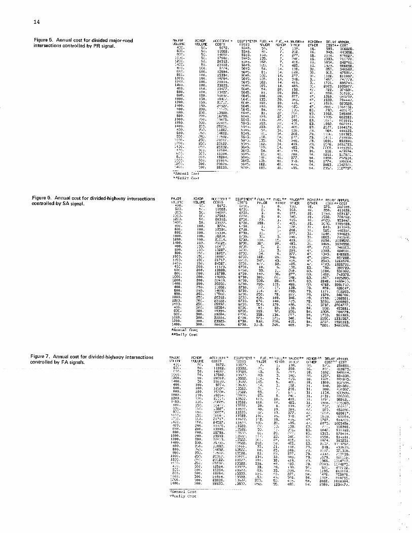
Figure 5. Annual cost for divided major-roadintersections controlled by PR signal.
IlAJORUOLUIIE
400,600.
l6e.t89.54,
.108.135.
r89.54.81.
108.135.164.189.54.81,
r 08.
185.54.81.
108.135.162.183.54.
108.135.t62.l8s,
5645.5645,5645.5645.
5645.5645,5645,5645,5645.
5645.
5645.5645,5645,5645.5645.5645,5645.5645.5645,5645.5645,5645.5645.5645.
5645.5645.5645,
I1âJOR ì1INOR ÊccIDENl* EOUP¡MENT*FUEL** FUEL** IAJoR** üINo;s** DELêV âN¡IUALuoLUriE uoLUrlE cosrs cg9ls mAJoR ¡rnoB orlÈB orHER ðósi** Cijõï-400. s0, 902¿. 6?30. t. 0. iss. 16. szs, eeãias.600. s0. UBB¿. qi30. e. 0. aõe. t6. Bso. ¡¡ioaõ:800. s0. l46s¿. q290, 3. o. azl, 16. riie. s-ãiãi.1000. s0. lzsoa. qi?q, B. 0. ¡ce. 16. rsse. iáoiø¿.re00. s0, e03la. 6230. e3. r, clã, 16, ¿083. s5ãca7.1400. s0. ¿3r?2. 873c. lsg. z, qai. 16. :o¡s, rã5s¿és.400. 100, ez?4. 6230. l. 0. rãe. 31. 643. ãiisã5,600. 100. rasg4. 6230. s. t. ãõB: 31. ses. i1sãoi.800. t00. ¡s3s4, 6730. 11, t. àzi, ã1: rããe. 6d46ãà:lqgS. r00. lB?04. 6230. 31, g. jqs, 31, l66a: ieist6:1e00. 100. at0r4. 6230. 184. ts. ct5. ai: ããéõ. loõàsäã.1400, r00. a3sas. 6230. 3a7. ¿8. ¿ai. ãi: -¡6s: i6ãããõB:400. lso. t04z?, 6230. s. a. rãe, 1i, iiã: -ã¡6õõã:
ÞgS. 150. t3esz.. 6230. lt. s. ãos. 47. looe, ieioõi,8û0. 1s0, 15092. 6730. 34, s. à27. 42. r34s. sisási.1000. lso. lgsoz. 6230. 166. ¿s. 345. 47. lgo4. asiã8s,1e00. tso. ¿rzr?. 6230. 34?. 43. its. 4?, as¿0. rãsssãs,1400. tso. z4sa?. 6730. s7z. 6e, cs5. 47, ¡õ¿ã: iõã#ãi:400. ?00. .u1zs. q230. t0. s. 13s. 63. zeã, áaãzãâ,600, ?00, t39as. qzqo. 33. lt. aoe. 63. roea. aãlàõã:800. ê00. 16299. 6230. t4e. 36, z?2, 63. l4sa. iaãai6.1000. e00. t960s. q¡39. 3oo. 60, 346, 63. 1s67. roê-ãò5:1e00. e00. ee4rs. 6?30. 5oB. Bs. 4rs. 63. ae¡e, ilssiiõ,1400. a00. asa30. 6230. z6s. tog. 4Bs. 63, czes. àælìiá,400. aso. lrgga. 6730. ?2. t?. t3B. zg. 8a6. 4¿Bó4i.600. eso. l46sa. 6730. ll4. 4?, eog. za: Llll: 6iããdä:800. ?s0. rzsoe. 6730. ¿s0, za. ???, zã. iS?õ: Bq6iã6:1000. a50. a03la. 6230. 43s. ro9. 346, ?9. eiss. riégà6i.l¿00. aso, a3tza. 6210. 620. t4o, 415. ?9, :eãe. i6s6e6s.1400. eso, es$a. qzgo, 9s4. r?0, 4Bs. zs, szsz. ãiÉ1iä,400. 300, r¿584. 6230, 8r. 60. l3B. s4. 93a, c5sàiri,600. 300. 1s394. ql9g. rss, sz. ?08. s4. ta6s. zoõ?is,s00. 300. tee04, q13g. 3sB. 134. ¿??. s4. iiõ-: séiàôã.1000. 300. et0l4, q¿qg, szt. t7L. 346. 94. esso. rããiÈ6i.1a00, 300, a38¿s. q290. 83¿, ¿08. ¡rÈ. s4. szsz. is6oi6à.1400. 300. a663s. 6230, ll4a. ¿4s. 4Bs, 94. zasr, iioiãis.
5. 485. t6. 1900, s675s4.3. 138. 31. 640, 324981,5. ¿08. 31. 900. 454307.7. ?7?, 31. 1164. 588586.9, 346. 31. 1431. 7¿6306.10. 415. 3r. 1704. 868421,12. 485. 31. 1984. 1015363,8, 138, 47. 707. 36010t.10, a08. 47. S70. 49ea96.13. e77. 47. 1237, 628617.15. 346. 47. 1509, 769e84,t8. 415. 47 , 1787. 914?¿3,20. 485. 47, ?073. 1065458.13. 138. 63. 777. 396e06.17. e08, 63. 104e. 531162.20. ?77, 63. 1313, 6?0414.?3. 346. 63. 15S0. 814lol,?7. 415. 63, ß?4, 963a51.30, 4e5. 63. 2t67, lll8a67.el. 138. 75, 848. 433533.e5. ¿08. 79, 1117, 57¡308.23. e77. 73. 139a. ?13733.33. 346. 73, 1675. 861332,38. 415. 73, 1966. 1014713.4?. 485. 79. ¿263, tt?4¿73.e9. 138. 94. 9¿1, 4?¿?32.35. e08. 34, 1195, 613110.40. ?77. 94. 1476. 759079.45, 346, 94, t765. 910755.50. 415, 94. e066. 1068904.55. 485. 94. a380. 123447e.
50,50,50.50.
100.100.100.10 0.l0 0.100.150.150.150.150.150.t50,¿00.e00.¿00.200.20 0.e00.250.250.250.250.250.250.300.300.300.300.300.300.
HÊJ0RUOLUIlE
400.6¡¡-800.
1000.1200.r400,400,600.800.
1000.1200.t400.400.600.800.
1000.120 0.140 0.400.600.800.
100 0.1¿00.1400.400.60t.800.
I 000.r e00.I 400.400.600.800.
r000,I 200.140ú.
7. 415,7. 485.
14. 138.14. e08.14. ?7?,t4. 345,14. 415.14. 485.20. l3B.e0. e08.20. ?77.e0. 346.20 . 415.a0, 485.47, 138.e7. 208.e7. 2?7.?7. 346,27 . 415.??. 485.34, 138.34. 208.
34. 346.34. 415.34. 485.4l, 138,4t. a08,41. e77.41. 346.41. 415.41. 4a5.
1e00.I 400.
40 0.600.80 0.
t000.120 0,¡400.400,600.800.
100 0.1a00.140 0.400.600.800,
1000,la00,I 400.400.60 0.80 0.
t000,1¿0 0.I 400.400,600.800.
100 0.1200.140 0.
50.50,
100,¡00,t00.¡ 00.t 00.t00.150.r50.150.150,150.150.20c.200.20 0.?00,200.200.250.e50.¿50.250.250.250.30 û.300.300,300,300.300.
3t ae.977 4.
1e584.15394.18e04.el014.23825.10477 .13487.16097.18907.?L7t?.245?7 .11179.r3989.16799,I9603.2¿419.25230,l r88¿.r469¿.17502.20312.23124.¿5934,12584.15394.18204.21014.e38e5,2663s.
.Figure 6. Annual cost for divided-highway intersectionscontrolled by SA signal,
Figure 7. Annual cost for divided-highway ¡ntersectionscontrolled by FA signals.
*Annual Cost**Da11y Cost
ffi**Dally Cost
T1INOR ÊCCIDENT* EOUPII1ENT * FUEL ** FUEL** ÍAJOR** íINOR** OELÊY ÊNNUALuoLUriE cosrs cosrs t1ÊJoR IrrNoR oIHER ornÈn aosi** Côsï-50. 907e. t35e2. 7. t. 138. 16. 573. 230Ss1
14692.17502,2031e.?312.
3??4.12584.15394.18e04.21014.238¿5.10477,
r6097.18907.?1717.?4527 .I I 173.13983,t6799.13609.2?4!3.25a30.I 188¿.r469¿.1750a,203 re,23rae.e593¿.12584.15394,18e04,2 r 014.e3845.26635.
135ae. 145.13524. M.13524. 31.13542. 55.
35?a, r68,35¿?, 20,35¿¿, 40.352¿. 67.352¿. 10 1.3522. t4?..35¿2. 190.3522. 27.3522. 50.352e. 81.35ee. 117.35¿e, 161,352e. atz.3522. 33-
60.13522. 60.135¿e. 93.135¿2, t34,135ae. r8l.l35e¿. 235.
l35ae. 69.135¿2, 106,I35ee. 150.1352¿. a00.135ee, 2sA.
*AnnuâI Cost**Daily Cost
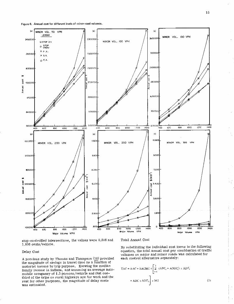
15
Figure 8. Annual cost for different levels of minor-road volumes.
MINOR VOL. IOO VPH
MINOR VOL. I5O VPH
MINOR VOL. 25O VPH MINOR VOL. 3OO VPHMINOR VOL. 2OO VPH
O
II
ECÊ E
400 6æ 800
Moior Volum€ VPH
stop-controlled intersections, the values were 0.806 and1.806 cents,/vehicle.
Delay Cost
A previous study by Thomas and Thompson (10) providedthe magnitude oi sávings in travel time as a Fnction ofmotorist income by trip purpose. Knowing the medianfamily income in Indiana, and assuming an average auto-mobile occupancy of 1.5 persons/vehicle and that one-third of the trips on rr.ral highways are for work and therest for other purposes, the magnitude of delay costswas estimated.
Total Annual Cost
By substituting the individual cost items in the followingequation, the total annual cost per combination of trafficvolumes on major and minor roads was calculated foreach control alternative separately:
fzTAC= AAC+ EACMC+I > 1ANC, + AOOC) X ADT¡
Li='
800 1000t{qior Volumt
t200 1400VPH
+ ADC x AorJ x 36s
800 1000
Moior Voluna
(l)
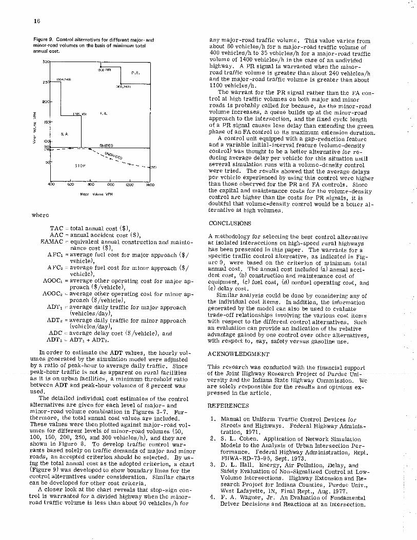
16
Figure 9. Control alternatives for different major- andminor-road volumes on the basis of min¡mum totalannual cosl.
any major-road traffic volume. This value varies fromabout 80 vehicles/h for a major-road traffic volume of400 vehicles/h to 35 vehicles/h for a major-road traffic
highway. A PR signal is warranted when the minor-road traffic vohDne is greater than about 240 vehicles/hand the major-road traffic volume is greater than about1100 vehicles/h.
The warrant for the PR signal rather than the FA con-trol at high traffic volumes on both major and minorroads is probably called for because, as the minor-roadvolume increases, a queue builds up at the minor-roadapproach to the intersection, and the fixed cycle lengthof a PR signal causes less delay than extending the greenphase of an FA control to its maximum extension duration.
A control unit equipped with a gap-reduction featureand a variable initial-interval feature (volume-densitycontrol) was thought to be a better alternative for re-ducing average delay per vehicle for this situation untilseveral simulation runs with a volume-density controlwere tried. The results showed that the average delaysper vehicle e:rperienced by using this control were higherthan those observed for the PR and FA controls. Sincethe capital and maintenance costs for the volume-densitycontrol are higher than the costs for PR signals, it isdoubtful that volume-density control would be a better al-ternative at high volumes.
CONCLUSIONS
A methodology for selecting the best control alternativeat isolated intersections on high-speed rural highwayshas been presented in this paper. The warrants for aspecific traffic control alternative, as indicated in Fig-ure 9, \¡/ere based on the criterion of minimum totalannual cost. The annual cost included (a) annual acci-dent cost, (b) construction and maintenance cost ofequipment, (c) fuel cost, (d) nonfuel operating cost, and(e) delay cost.
Similar analysis could be done by considering any ofthe individual cost items. In addition, the informationgenerated by the model can also be used to evaluatetrade-off relationships involving the various cost itemswith respect to the different control alternatives. Suchan evaluation can provide an indication of the relativeadvantage gained by one control over other alternatives,with respect to, say, safety versus gasoline use.
In order to estimate the ADT values, the hourly vol- ACKNOWLEDGMEIIT'umes generated by the simulation model were adjustedby a ratio of peak-hour to average daily traffic. Since This research was conducted with the financial supportpeak-hour traffic is not as appa+ent-on rulal faeiliÈies of the .Ioht Highway Research project of purdurUni-as it is on urban facilities, a minimum threshold ratio versity and thã Indiâna State Highwäy Commission. Webetween ADT and peak-hour volumes of I percent was are soiely responsible for the rãsults and opinions ex-used. pressed in the article.
The detailed individual cost estimates of the controlalternatives are given for each level of major- andminor-road volume combination in Figures 3-7. trirr-thermore, the total annual cost values are included.These values were then plotted against major-road vol-umes for different levels of minor-road volumes (b0,100, 150, 200, 250, and 300 vehicles/h), and they areshown in Figure L To develop traffic control war-rants based solely on traffic demands of major and minorroads, an accepted criterion should be selected, By us-ing the total annual cost as the adopted criterion, a chart(Figure 9) was developed to show bìundary lines for thecontrol alternatives under consideration. Similar chartscan be developed for other cost criteria,
A closer look at the chart reveals that stop-sign con-trol is warranted for a divided highway when the minor-road traffic volume is less than about g0 vehicles/h for
TÀ
E
g
.s
where
TAC = total annual cost ($),AAC = annual accident cost ($),
EAMAC = equivalent annual construction and mainte-nance cost ($),
AFCr = average fuel cost for major approach ($/vehicle),
AFCz = average fuel cost for minor approach ($/vehicle),
AOOCr = averâge.other operating cost for major ap-proach ($/vehicle),
AOOC¿ = âverage other operating cost for minor ap-proach ($/vehicle),
ADT1 = average daily traffic for major approach(vehicles/day),
ADT¿ = average daily.traffic for minor approach(vehicles,/daY),
ADC = average delay cost ($/vehicle), andADTg=ADTr+ADT¿,
REFERENCES
1. Manual on Uniform Traffic Control Devices forStreets and Highways. Federal Highway Adminis-tration, 1971.
2. S. L. Cohen. Apptication of Network SimulationModels to the Analysis of Urban Intersection per-formance. Federal Highway Administration, Rept.FHWA-RD-?3-95, Sept. 1973.
3. D. L. Hall. Energy, Air Pollution, Delay, andSafety Evaluation of Non-Signalized Control at Low-Volume Interseetions, Highway Extension and Re-search Project for Indiana Counties, Purdue Univ.,West Lafayette, IN, Final Rept., Aug. 197?.
4. F. A. Wagner, Jr. An Evaluation of FUndamentalDriver Decisions and Reactions at an Intersection.
--_$tu,oo
sroP \.* \ -
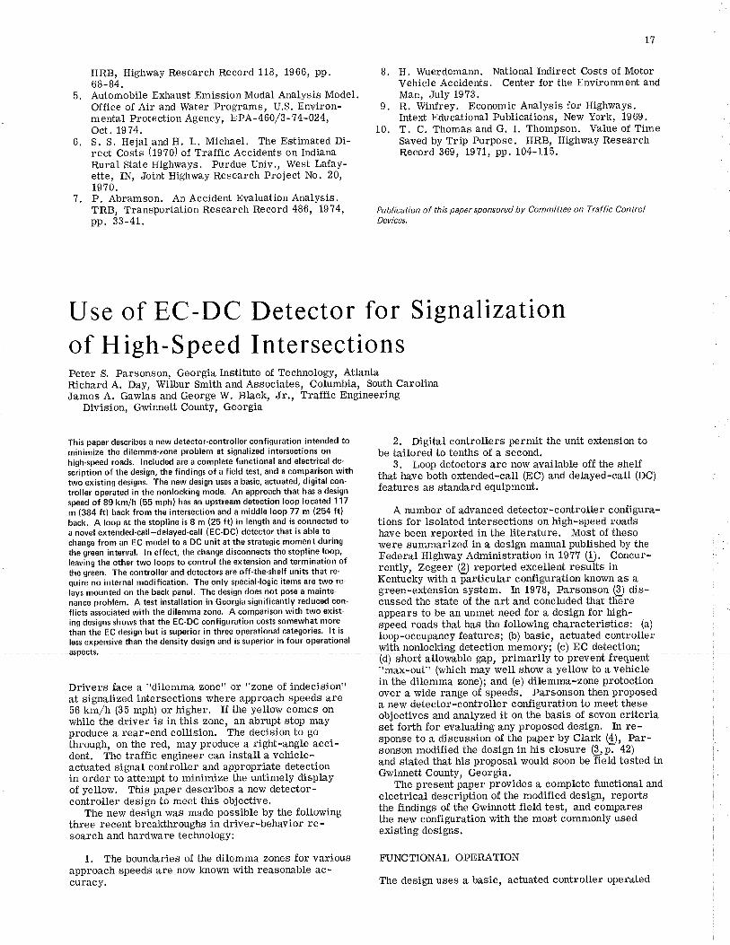
HRB, Highway Research Record 118, 1966, pp.6B-84.
5. Automobile Exhaust Emission Modal Analysis Model.
mental Protection Agency, EPA-460/3-74-024,Oct.1974.
6. S. S. Hejal and H. L. Michael. The Estimated Di-rect Costs (1970) of Traffic Accidents on IndianaRural State Highways. Purdue Univ., West Lafay-ette, IN, Joint Highway Research Project No. 20,1970.
'l . P. Abramson. An Accident Evaluation Analysis.TRB, Transportation Research Record 486, t974,pp. 33-41.
L7
8. H. Wuerdemann. National Indirect Costs of MotorVehicle Accidents. Center for the Environment andMan, July 1973.
Intext Educational Publications, New York, 1969.10. T. C. Thomas and G. I. Thompson. Value of Time
Saved by Trip Purpose. HRB, Highway ResearchRecord 369, 1971, pp, 104-115.
Publicatìon of this paper sponsored by Comm¡ttee on Traffic ControlDevices.
Use of EC-DC Detector for Signallzatton
Peter S. Parsonson, Georgia Institute of Technology, AtlantaRichard A. Day, Wilbur Smith and Associates, Columbia, South CarolinaJames A. Gawtas and George W. Black, Jr., TrafÏic Engineering
Division, Gwi¡¡nett County, Georgia
of High-Speed Intersections
This paper describes a new detector-controller configuration ¡ntended tominimize the d¡lemma-zone problem at signalized ¡ntersections onhigh-speed roads. lncluded are a complete funct¡onal and electrical de-
script¡on of the des¡gn, the findings of a field test, and a comparison withtwo existing designs. The new design uses a basic, actuated, digital con-
troller operated in the nonlocking mode. An approach that has a design
speed of 89 km/h (55 mph) has an upstream detection loop located 1 17
m (384 ft) back from the intersection and a middle loop 77 m (254 ft)back. A loop at the stopline ¡s 8 m (25 ft) in length and is connected toa novel extended-call-delayed-call (EC-DC) detector that ¡s able tochange from an EC model to a DC unit at the strategic moment duringthe green interval. ln effect, the change disconnects the stopline loop,leav¡ng the other two loops to control the extension and termination offüe green. The controller and detectors are off'the-shelf un¡ts that re-
quire no internal modification. The only special-logic ¡tems are two re-
lays mounted on the back panel. The design does not pose a ma¡nte'nance problem. A test ¡nstallat¡on in Georgia significantly reduced con-flicts associated with the dilemma zone' A comparison with two exist-ing designs shows that the EC-DC configuration costs somewhat morethan the EC design but is superior ¡n three operational categor¡es. lt ¡s
less expensive than the density design and is superior in four operational
Drivers face a "dilemma zone" or "zone of indecision"at signalized intersections where approach speeds are56 km/h (35 mph) or higher. If the yellow comes onwhile tlre driver is in this zone, an abrupt stop mayproduce a rear-end collision. The decision to gothrough, on the red, may produce a right-angle acci-dent. The tra"ffic engineer can install a vehicle-actuated signal controller and appropriate detectionin order to attempt to minimize the untimely displayof yellow. This paper describes a new detector-controller design to meet this objective.
The new design was made possible by the followingthree recent breakthroughs in driver-behavior re-search and hardware technology:
1. The boundaries of the dilemma zones for variousapproach speeds are now knorvn with reasonable ac-curacy.
2, Digital controllers permit the unit extension tobe tailored to tenths of a second.
3. Loop detectors are now available off the shelfthat have both extended-call (EC) and delayed-call (DC)features as standard equiPment.
A number of advanced detector-controller confígura-tions for isolated intersections on high-speed roadshave been reported in the literature. Most of thesewere summarized in a design manual published by theFederal Highway Administration in 1977 (!. Concur-rently, Zegeer @) reported excellent results inKentucky with a particular configuration known as agreen-extension system. In 1978, Parsonson (Q dis-cussed the state of the art and concluded that thereappears to be an unmet need for a desígn for high-speed roads that has the following characteristics: (a)loop-occupancy features; (b) basic, actuated controllerwith nonlocking detection memory; (c) EC detection;(d) short atlowable gap, primari þevenI-requen-"max-out" (which may well show a yellow to a vehiclein the dilemma zone); and (e) dilemma-zone protectionover a wide range of speeds. Parsonson then proposeda new detector-controller configuration to meet theseobjectives and analyzed it on the basis of seven criteriaset forth for evaluating any proposed design. In re-sponse to a discussion of the paper by Clark $), Par-sonson modified the design in his closure Qrp. a2)and stated that his proposal would soon be field tested inGwinnett County, Georgia.
The present paper provides a complete functional andelectrical description of the modified design, reportsthe findings of the Gwirmett field test, and comparesthe new configuration with the most commonly usedexisting designs.
FUNCTTONAL OPERATION
The design uses a basic, actuated controller operated
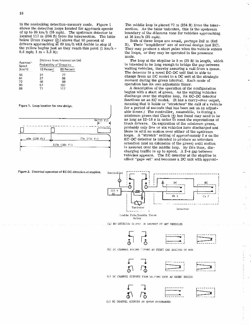
18
in the nonlocking detection-memory mode. Figure I
ApproachSpeed(km/h)
below ürom Zegeer @J shows ihat 90 percent ofdrivers approaching at 89 km/h rvill decide to stop ifthe yellow begins just as they reach tlris point (1 km/h =0.6mph;1m=3.3ft):
Distance from lntersection (m)
The middle loop is placed 77 m \254 ft) from the inter-section. As the table indicates, this is the upstreamboundary of tåe dilemtna zone for vehicles approaching
Both of these loops are small, perhaps 2x2 m (6x6ft). Their "amplifiers" are of normal design (not EC).They may produce a short pulse when the vehicle entersthe loops, or they may be operated in the presencemode.
The loop at the stopline is 8 m (2õ ft) in length, whichis intended to be long enough to bridge the gap betweenwaiting vehicles, thereby assuring a call from a queue.The detector is a novel EC-DC unit that is able tochange from an EC model to a DC unit at the strategicmoment during the green interval. Each mode ofoperation has its own adjustable timer.
A description of the operation of the configurationbegins with a start of green. As the waiting vehiclesdischarge over the stopline loop, its EC-DC detectorfunctions as an EC model. (It has a carry-over output,meaning that it holds or "stretches" the call of a vehiclefor a period of seconds that has been set on an adjust-able timer.) The controller, meanwhile, is timing aminimum green that Cfark (S has found may need to beas long as 12-18 s in order lo meet the enpectations oftruck drivers. On expiration of the minimum green,probably only five or six vehicles have discharged andthere is still no motion over either of the upstreamloops. A "stretch" setting of approximately 2 s on theEC-DC detector is intended to produce an unbrokenactuation (and an extension of the green) until motionis assured over the middle loop. By this time, dis-charging tra-ffic is up to speed. A 2-s gap betweenvehicles appears. The EC detector at the stoptine ineffect "gaps out" and becomes a DC unit with approxi-
DetecÈor
Probabil ity of Stopping
10 Percent 90 Percent
5664728089
3137465271
778699
107117
Figure 2, Electricâl operation of EC.DC detection at stopline.
Double Pole/Double ThrowRelay
Loop location for new design.
77û (254 ftl17n (384 ft)
EC--- -------l
-rl
.------;-.ji----i
(b) DC CHANNEL BEGINS TIMING AS TIRST CAR ARRIIES ON RED
II
II
_-t
F__i(d) Ec
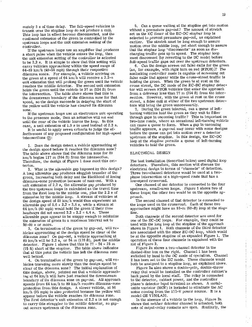
mately 5 s of time delay. The fuIl-speed vehicles intransit over the stopline loop do not produce a call.
19
5. Can a queue waiting at the stopline get into motionwittrout a premature gap-out? The amount of stretchset on the EC timer of the EC-DC stopbar loop isbecome disconnected. and the
continued extension of the green is controlled byupstream loops and tj¡e unit extension setting of thecontroller.
If tl¡e upstream loops use an amplifier that producesa short pulse when ttre vehicle enters the loop, thenthe unit extension setting of the controller is selectedtobe 2.2 s. It is simple to show t¡at thÍs settÍng willcarry vehicles approaching within the speed range of64-89 km/h (40-55 mph) through their respectivedílemma zones. For e>rample, a vehicle arriving onthe green at a speed of 64 km/h will receÍve a 2,2-sunit extension that will prolong the green until the vehiclereaches the middle detector. The second unit extensionholds the green until the vehicle is 37 m (124 ft) fromthe intersection. The table above shows tÌ¡,at this isthe downstream boundary of the dilemma zone for thatspeed, so the design succeeds ín delaying the start ofthe yellow until the vehicle has cleared its dilemmazoîe.
If the upstream loops use ar electronics unit operatingÍn the presence mode, tùen a¡ actuation will not enduntil the rear of the vehicte leaves the loop. In thiscase, a unit e*ension of 1.9 s is used instead of 2.2 s.
It'is useful to apply seven criteria to judge the ef-fectiveness of any proposed configtrration for high-speedintersections ($:
1. Does the design detect a vehicle approaching atthe design speed before it reaches the dilemma zone?The table above shows that the dilemma zone for 89
km/h begins 117 m (384 ft) from the intersection.Therefore, the design of Figure 1 does meet this cri-terÍon.
2, What is the allowable gap imposed by this design?A long allowable gap produces sluggish transfer of thegreen, increasing both delay and the likelihood of losingdilemma-zone protection because of max-out. \¡fith aunit extension o1.2.2 s, the allowable gap produced bythe two upstream loops is calculated as the travel timefrom the first loop to the middle one, plus the 2.2 s ofextension by the middle loop. A stream of vehicles atthe design speed of 89 km/h would thus e4perience anallowable gap of 1.6 + 2.2 = 3.8 s, while a stream at64 km/h (40 mph) would hold the green if their tÍmeheadways did not exceed 2.2 + 2.2 = 4,4 s. Theseallowable gaps appear to be snappy enough to minimizethe extension of green to a maximum interval set to
prevent preearlier. The stretch must be long enough to assuremotion over tlre middle loop, yet short enough to assuretirat the stopbar loop "disconnects" as soon as dis-charging traffic gets up to speed. The stopbar loopmust discornect þy reverting to the DC mode) beforefull-speed tra-ffic gaps out over the upstream detectors.
6. Ca¡ the design screen out false calls for the greenhs, for example, with right turn on red (RTOR)J? Thenonlocking controller mode is capable of screening outfalse calls that appear while ttre cross-street tra-ffic isholding the green. When ttre green is at rest on thecross street, the DC mode of the EC-DC stopbar detec-tor will screen RTOR vehicles that enter the approachfrom a driveway less than 77 m (264 ft) from the inter-section. However, with the green at rest on the crossstreet, a false call at either of the two upstream detec-tors will bring the green unnecessarily.
1, During the green interval, can a queue of left-turning vehicles hold the green as they wait to filterthrough gaps in oncoming tra-ffic? This is important ontwo-lane roads, where an occasional left-turning vehiclecan cause a queue to form. When a gap in oncomingtraJfic appears, a gap-out may occur vr¡ith some designsbefore the queue can get into motion over a detectorupstream of the stopline. In tlris design, the EC-DCloop at the stopline permits a queue of left-turningvehicles to hold the green.
ELECTRICAL DESÍGN
The test installation (described below) used digital loopdetectors. Therefore, this section rvill discuss theelectrical design in terms of "channels" of detection.Three two-chan¡el detectors would be used at a two-phase intersection of a high-speed route that has alow-speed crossroad.
One char¡nel of one detector is connected to the fourupstream, small-area loops. Figure 1 sho"vs two ofthese loops; the other two would be on the opposite ap-proach.
The second channel of that detector is cormected tothe loops used on the crossroad. Each of these twoapproaches might have an 18-m (60-ft) loop at tlte stop-line.
Both charurels of the second detector are used forone of the EC-DC loops. For example, they could be
.60 s or more. used rvith the long loop at the stopline of the approach3. g¡¡ ¡s¡min¿¡ien of the green by gap-ou
5O-ßO s ôr môre-
hicles approaching at the design speed be clear of the are associated with the other EC-DC loop, which woulddilemmã zone? On gap-out, á vehicle approaching at be at the opposite stopline of an expanded Figure 1. The89 km/h will be 2.2 sr- or 54 m (1?8 ft), past the middle operation of these four eharurels Ís explained with thedetector. Figure 1 shows that this is 7? - 54 = 23 m aid of Figure 2.(?5 ft) short of tlle stopline. The table above indicates Figure 2a shows a two-channel detector in thedt¡at at this point the vehicle has teft the dilemma zone dashed-line box on the right. Charurel t has been
rvell behind. srvitched by hand to ttre DC mode of operation. Channel4. On termination of the green by gap-out, will ve- 2 has been set to the EC mode. These charnels would
hicles traveling more slowly than the design speed be both be assigned to a stopline loop, as ex¡plained above.clear of the dilemma zone? The initial erçlanation of Figure 2a also shows a double-pole, double-throwthis design. above, pointed out that a vehicle approach- relay that would be installed on the controller cabinet'sing at 64 kiir/h will have just reached the downstream back panel by the local staff. The relay is cornectedboundary of its dilemma zon¡e on gap-out. AI1 approach to t}re detector, cabinet power, and the controllerspeeds from 64 km/h to 89 km/h receive dilemma-zone phase's detestor input terminal as shown. A metal-protection from this design. A slower vehicle, at 56 oxide varÍstor (MOV) Ís included to eliminate the ACÌ<m/ir (¡S mph) is also protected because the yellow will noise coming from the 115-V power source. It is aappear before the vehicle reaches its dilemma zone. model GE V150L420.The first detector's unit extension ot 2,2 s is not enough In the absence of a vehicle in the loop, Figure 2ato carry this straggler to the middle detector, so gap- shows that neitler detector cha¡urel is actuated; bothout occurs upstream of the dilemma zone. sets of output-relay contacts are open. Similarly, the
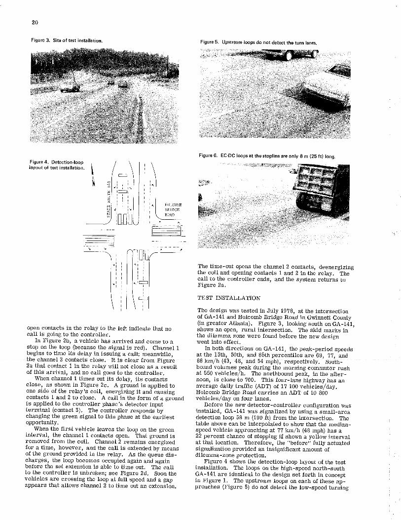
20
Figure 3. Site of test installat¡on. Figure 5. Upstream loops do.not detect the turn lanes.
Figure 4. Detect¡on-looplayout of test installation,
-_-.- -; --- --
I
lvI
I
l"I
\
\
open contacts in the relay to the left indicate that nocall is going to the controller.
In Figure 2b, a vehicle has amived and come to astop on the loop þecause the signal is red). Channel 1begins to time its delay in issuing a call; meanwhile,
Jhe ehannel 2 contacts close. It is clear from Figure2athat contact 1 in the retay will not close as a resultof this arrival, and no call goes to the controller.
When charmel 1 times out its delay, its contactsclose, as shown in Figure 2c. A ground is applied toone side of the relay's coil, energizingit and causingcontacts 1 and 2 to close. A call in the form of a groundis applied to the controller phase's detector inputterminal (contact 3). The controller responds bychanging the green signal to this phase at the earliestopportunity.
When the first vehicle leaves the loop on the greeninterval, the channel 1 contacts open. That ground isremoved from the coil. Charu¡el 2 remains energizedfor a time, however, and the call is extended by meansof the ground provided in the relay. As the queue dis-charges, the loop becomes occupied again and againbefore the set extension is able to time out. The callto the controller is unbroken; see Figure 2d, Soon thevehicles are crossing the loop at full speed and a gapappears that allows chaûiet 2 to time out an extension.
Figure 6. EC-DC loops at the stopl¡ne are only I m (25 ft) long.
#+
)
The time-out opens the charurel 2 contacts, deenergizingthe coil and opening contacts 1 and 2 in the relay. Thecall to the controller ends, and the system returns toFigure 2a.
TEST INSTALLATION
The design',vas tested in July 1g?8, at the intersectionof GA-141 and Holcomb Bridge Road in Gwi¡rrett County(in greater Atlanta). Figure 3, looking south on GA-141,shows an open, rural intersection. The skid marks inthe dilemma zone were found before the new designwent into effect.
In both directions on GA-141, the peak-period speedsat the 15th, 50th, and BSth percentiles are 6g, ??, and86 kmlï (43, 48; ãrd 54 mph), respeõtivGly. Soufh-bound volumes peak during the morning commuter rushat 550 vehicles/h. The northbound peak, in the a-fter-noon, is close to 700. This four-la¡e highway has anaverage daily traffic (ADT) of 1? 100 vehicles/day.Holcomb Bridge Road carries an ADT of 10 800vehicles/day on four 1anes.
Before the new detector-controller configuration wasinstalled, GA-141 was signalized by using a sma-ll-areadetection loop 58 m (190 ft) from the intersection. Thetable above can be interpolated to show thai the median-speed vehicle approaching at 77 km/h (49 mph) has a22 percent chance of stopping if shown a yellolv intervalat that location, Therefore, the "before" fully actuatedsignalization provided an insignificant amount ofdilemma-zone protection.
Figure 4 shows the detection-loop layout of the testinstallation. The loops on the high-speed north-southGA-141 are identical to the design set forth in conceptin Figure 1. The upstream loops on each of these ap-proaches (Figure 5) do not detect the low-speed turning
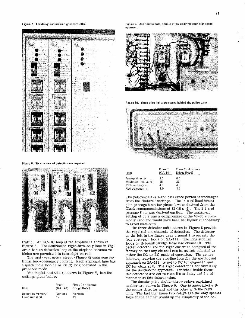
2t
Figure 7. The design requires a digital controller. Figure 9. One double-pole, double"throw relay for each high-speedapproach.
O-...o..".^'
-0":':::
ilr**
H
O-...a'.-..'-
_.*'-
ilrr*
M i¡,;I
oooo
Figure 8. Six channels of detection are required,
traffic. An EC-DC loop at the stopline is shown inFigure 6. The southbound right-turn-only lane in Fig-ure 4 has no detection loop at the stopline because ve-hicles are permitted to turn right on red.
The east-west cross street (Figure 4) uses conven-tional loop-occupancy control. Each approach lane hasa quadrupole loop 18 m (60 ft) long operated in thepresence mode.
The digital controller, shown in Figure 7, has thesettings given below.
Figure 10. Three pilot l¡ghts are stored behind the police panel.
Phasel Phase2(Holcomb(GA-141) Bridge Road)
Passage time (s)
Maximum interval (s)
Yellow change (s)
Red clearance (s)
2.2554.31.5
0.5354.31.7
The yellow-plus-all-red clearance period is unchangedfrom the "before" settings. The 14 s of fixed initialplus passage time for phase 1 were derived from theClark recommendations of 12-18 s ($. The 2.2 s ofpassage time was derived earlier, The maximumsetting of 55 s was a compromise of the 50-60 s com-monly used and would have been set higher if necessaryto avoid max-outs.
The three detector units shown in Figure I providethe required six channels of detection. The detectoron the left in the figure uses channel 1 to operate thefour upstream loops on GA-141. The long stoplineloops on Holcomb Bridge Road use charmel 2. Thecenter detector and the right one were designed at thefactory so that any channel can be switch-selected toeither the DC or EC mode of operation. The centerdetector, serving the stopline loop for the northboundapproach on GA-141, is set to DC for channel 1 andEC for charurel 2. The right detector is set similarlyfor the southbound approach. Slitches inside thesetwo detectors are set to time 5 s of delay and 2 s ofextension at this intersection.
The double-pole, double-throw relays e¡plainedearlier are shown in Figure 9. One is associated withthe center detector unit and the other with the riehtunit. The fact that these two relays are the only speciallogic in the cabinet points up the simplicity of the de-
Item
ItemPhasel Phase2(Holcomb(cA-141) Bridse Road)
Detection memory Nonlock NonlockFixed initial (s) 12 12
ffi'
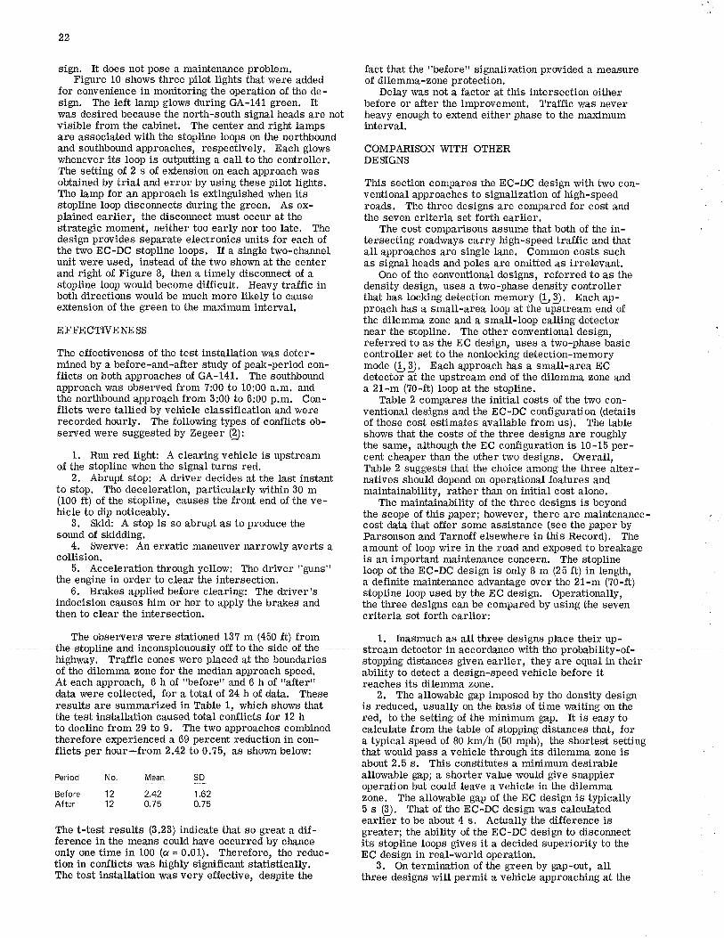
síTn- The lefË þrnp Slews dErinÊ GA-141 Sreen; It before or after tl¡e improvement; Trwas desired because the north-south signal heads are not heavy enough to extend either phase to the maximum
22
sign. It does not pose a maintenance problem.Figure 10 shows three pilot lights that were added
for convenience in monitoring the operation of tJre de-
visible from the cabinet. The center and right lampsare associated with the stopline loops on the northboundand southbound approaches, respectively. Each glowswhenever its loop is outputting a call to the controller.The setting of 2 s of extension on each approach wasobtained by trial and error by using these pilot lights.The lamp for an approach is extinguished when itsstopline loop disconnects during the green. As ex-plained earlier, the discormect must occur at thestrategic moment, neither too early nor too late. Thedesign provides separate electronics units for each ofthe two EC-DC stopline loops. If a single two-charnelunit were used, instead of the two shown at the centerand right of Figure 8, then a timely discormect of astopline loop would become di-fficult. Heavy traffic inboth directions would be much more likely to causeextension of the green to the maximum interval.
EFFECTTVENESS
The efïectiveness of the test installation was deter-mined by a before-and-after study of pea}-period con-flicts on both approaches of GA-141. The southboundapproach was observed from 7:00 to 10:00 a.m. andthe northbound approach from 3:00 to 6:00 p.m. Con-flicts were tallied by vehicle classification arid wererecorded hourly. The following types of conflicts ob-served lvere suggested by Zegeer (þ:
1. Run red light: A clearingvehicle is upstreamof the stopline when the signal turns red.
2. Abrupt stop: A driver decides at the last instantto stop. The deceleration, particularly within 30 m(100 ft) of the stopline, causes the front end of the ve-hicle to dip noticeably.
3. Srid: A stop is so abrupt as to produce thesound of skidding.
4. Swerve: An erratic m¿ùneuver namowly averts acollision.
5. Acceleration through yellow: The driver "guns"the engine in order to clear the intersection,
6. Brakes applied before clearing: The driver'sindecision causes him or her to apply the brakes andthen to clear the intersection.
The observers were stationed 137 m (450 ft) fromthe stopliae and ineonspieuousl¡sff ts the side of thehighway. Tra-tfic cones were placed at the boundariesof the dilemma zone for the median approach speed.At each approach, 6 h of "before" and 6 h of "after"data were collected, for a total of 24 h of data. Theseresults are sumûErized in Table 1, which shows thatthe test installation caused total co¡¡flicts for 12 hto decline from 29 to 9. The two approaches combinedtherefore experienced a 69 percent reduction in con-flicts per hour-from 2.42 to 0.75, as shown below:
Period No.
Before 12After 12
SD
1.620.75
The t-test results (3.23) indicate that so great a dif-ference in the means could have occurred by chanceonly one time ir 100 (a = 0.01). Therefore, the reduc-tion in co¡rflicts was highly significant statistically.The test installation was very effective, despite the
fact that the "before" signalization provided a meaÉiureof dilemma-zone protection.
Delay was not a factor at this intersection either
interval.
COMPARISON WITH OTHERDESIGNS
This section compares the EC-DC design with two con-ventional approaches to signalization of high-speedroads. The three designs are compared for cost andthe seven criterÍa set forth earlier.
The cost comparisons assume that both of the in-tersecting roadways carry high-speed tra.ffic and thatall approaches are single lane. Common costs suchas sigrnl heads and poles are omitted as irrelevant.
One of the conventional designs, referred to as thedensity design, uses a two-phase density controllerthat has locking detection memory [, S. Each ap-proach has a small-area loop at the upstream end ofthe dilemma zone and a small-loop calling detectornear the stopline. The other conventional design,referred to as the EC design, uses a two-phase basiccontroller set to the nonlocking detection-memorymode $S. Each approach hås a small-area ECdetector at the upstream end of the dilemma zone andaZt-m (70-ft) loop at the stopline.
Table 2 compares the initial costs of the two con-ventional designs and the EC-DC configuration (detaitsof these cost estimates available from us). The tableshows that the costs of the three designs are roughlythe same, although the EC configuration is 10-15 per-cent cheaper tltan the other two designs. Overall,Table 2 suggests that the choice among the three alter-natives should depend on operational features andmaintainability, rather tha¡ on initial cost alone.
The maintainability of the three designs is beyondthe scope of this paper; however, there are maintenance-cost data that offer some assistance (see the paper byParsonson and Tarnoff elsewhere in this Record). Theamount of loop wire in the road and e:çosed to breakageis an important maintenance concern. The stoplineIoop of the EC-DC design is only I m (25 ft) in length,a definite maintenance advantage over the 21-m (70-ft)stopline loop used by the EC design. Operationally,the three designs can be compared by using the sevencriteria set forth earlier:
1. Inasmuch as all three designs pl,ace their up-stream detectorin accordance witù theprobabilitf-of-stopping distances given earlier, they are equal in theirability to detect a design-speed vehicle before itreaches its dilemma zone.
2. The allowable gap imposed by the density designis reduced, usually on the basis of time waiting on thered, to the setting of tìe minimum gap. It is easy tocalculate from the table of stopping distances that, fora typical speed of 80 km/h (50 mph), the shortest settingthat would pass a vehicle through its dilemma zone isabout 2.5 s. This constitutes a minimum desirableallowable gap; a shorter value would give snappieroperation but could leave a vehicle in the dilemmazone. The allowable gap of the EC design is typically5 s (Ð. That of the EC-DC design was calculatedearlier to be about 4 s. Actually the difference ísgreater; the ability of the EC-DC design to disco¡mect l
íts stopline loops gives it a decided superiority to theEC design in real-world operation.
3. On termination of the green by gap-out, allthree designs will permit a vehicle approaching at the
Mean
2.420.75
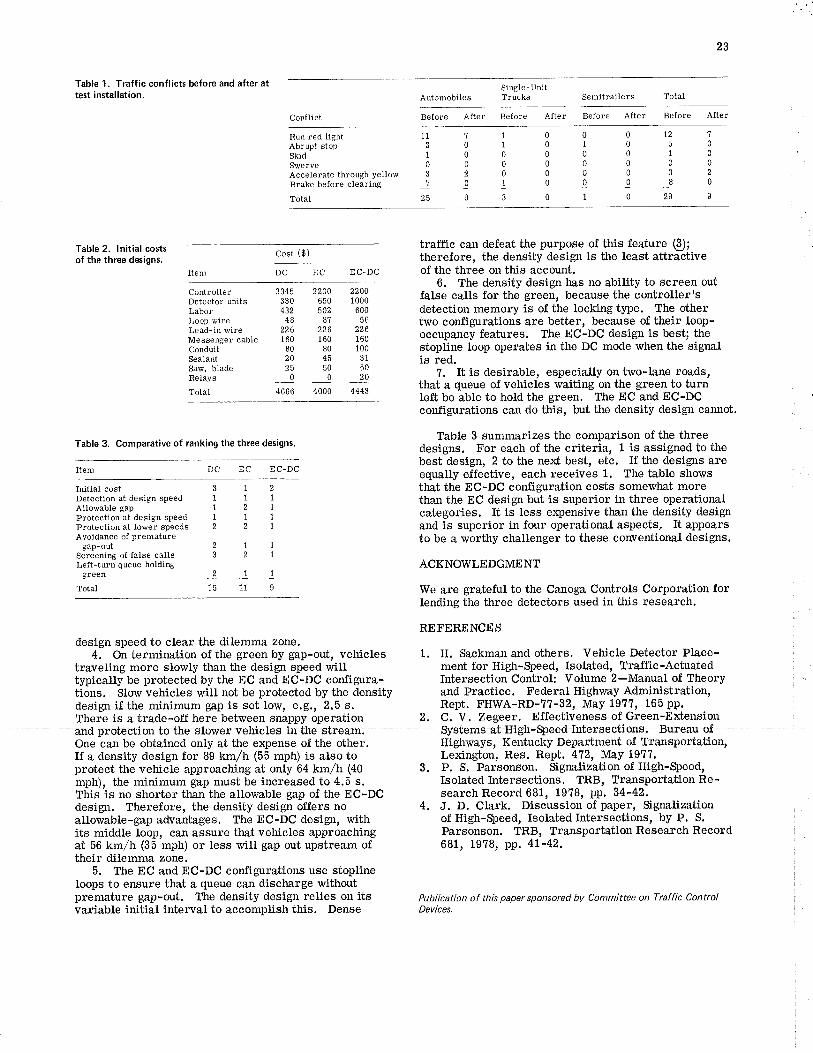
23
Table 1. Traffic conflicts before and after attest installat¡on.
Table 2. lnitial costsof the three des¡gns.
Item
CôntrollerDetector unitsLaborLoop wireLead-in wireMessenger cableConduitSealantSâw, bladeReIays
Total
Initial costDetection at desÍgn speedAllowable gapProtection at design speedProtection at lower speedsAvoidânce of premature
gap-outScreening of false callsLeft-turn queue holding
green
Total
AutomobilesSingle-UnitTrucks Semitrailers Total
Run red lightAbrupt stopskidSwerveAccelerate through yellowBrake before clearing
Totâl
12 'l501000328_q
299
11 ',l
3010007_q
259
0010000000q!10
10100000001-q30
Table 3. Comparative of ranking the three designs.
DC EC EC-DC
1
1
1
2
traffic can defeat the purpose of this feature (S;therefore, the density design is the least attractiveof the three on this account.
6. The density design has no ability to screen outfalse calls for the green, because the controller'sdetection memory is of the locking type. The othertwo configurations are better, because of their loop-occup¿ulcy features. The EC-DC design is best; thestopline loop operates in the DC mode when the signalis red.
1. It is desirable, especially on two-lane roads,that a queue of vehicles waiting on the green to turnleft be able to hold the green. The EC and EC-DCconfigurations can do this, but the densÍty design carmot.
Table 3 summarizes the comparison of the threedesigns. For each of the criteria, 1 is assigned to thebest design, 2 to the next best, etc. If the designs areequally effective, each receives 1. The table showsthat the EC-DC configuration costs somewhat morethan the EC design but is superior in three operationalcategories. It is less expensive than the density desigrtand is superior in four operational aspects. It appearsto be a worthy challenger to these conventional designs.
ACKNOWLEDGMENT
We are grateful to the Canoga Controls Corporation forlending the three detectors used in this research.
REFERENCES
1. H. Sackman and others. Vehicle Detector Place-ment for High-Speed, Isolated, TraffÍc-ActuatedIntersection Control: Volume 2-Manual of Theoryand Practice. Federal Highway Administration,Rept. FIIWA-RD-77-32, May 1977, 165 pp.
2, C. V. Zegeer. Effectiveness of Green-Extension
Cost ($)
EC EC-DC
3345 2200330 650432 50248 8?
226 226160 16080 8020 4525 5000
4666 4000
22001000
60056
226160100
5020
4443
l2112L112L
21132121!
15119
design speed to clear the dilemma zone.4. O¡r termination of the green by gap-out, vehicles
traveling more slowly than the design speed willtypically be protected by the EC and EC-DC configura-tions. Slow vehicles will not be protected by the densitydesigrr if the minimum gap is set low, e.g., 2.5 s.There is a trade-off here between snappy operation
TrotectÍonn fothrslourerrrehiclerlrrthestream; stems at lÌigh-$peed lnterseetioas. Bureau ofOneìan be obtained only at the expense of the other. Highways, Kentucky Department of Transportation,If a density design for 89 km/h (55 mph) is also to Lexington, Res. Rept. 412, lvlay 1977.protect the vehicle approaching at onfu b¿ tm/tr (+O 3. P. S. Parsonson. Signalization of High-Seed,mph), the minimum gap must be increased to 4.5 s. Isolated Intersections. TRB, Transportation Re-fñidis no shorter than the allowable gap of the EC-DC search Record 681, 1978, pp. 34'42.design. Therefore, the density design offers no 4. J. D. Clark. DiscussÍon of paper, Signalizationallowable-gap advantages. The EC-DC design, wÌth of High-SBeed, Isolated Intersections, by P. S.
its middle loop, can assure that vehicles approaching Parsonson. TRB, Transportation Research Recordat 56 km/h (35 mph) or less will gap out upstream of 681, 1978, pp. 41-42.their dilemma zone.
5. The EC and EC-DC configurations use stoplineloops to ensure that a queue can discharge wit}outpremature gap-out. The density design relies on its Pubtication of this paper sponsored by Committee on Traffic Con¡olvariable initial interval to accomplish this. Dense Devices.
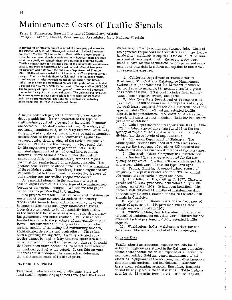
24
Maintenance Costs of Traffic SignalsPhilip J. TarnofÏ, Álao À4,-Voorhees and associatãs, Inc., Mclean, Virginia
develop guidelines for the selection of the type of ïl-iltra-ffÍc-sìgnal control to be used at individuàllnánintu"- years were obtained'coru¡ected or "isolated") intersections. 1'ne choice of ^^-';-
Ohio Department of Trans^por!1li-on (DOT): Ohiopretimed, semiactuated, basic fully actuatea,
-o" au*itv DoT furnished approximate data for 1976 on the fre-
iullyactuâtedsisnats weíehsthe tow price ;ri"d;#;ä gT9,_tg of repair of their 558 actuated trafTic signals,mainrenance or [he pretiried conrroúers asai'rãt-iüã-'--*- divided
iülilrjffåB:ilir",1j,irtii"åliiiii;, ,r"reduced costs, delays, etc., of the tra-tfic-responsive .., ]:-models. The staff óf ihe
"eiearch project t"rriJtrr"t- Minneapolis District furnished data co¡¡ering several
tra-tfic engineers generally prefer tã instatt tuú.*- I_"1,1: -fo" the frequency of repair of 135 actuated con-
actuated slgnat co;trol at individual intersectiils. trollers and several hundred detectors of various types.However, there is some concern over tfte cosioî' 5: 9iitirmlþ lttio: Computerized maintenance
maintainíng fully actuated controls, rvNch is ftign"" summ¿ries tot 272 years were obtained for the fre-ihan that for semiactuated or pretiíned
"o"t"ol"l..änu gu:nc,y of repair of more than 700 controllers and their
professional literature sheds iitge light on tir" *ug-ttifu¿" detectors, which were of various types and ages.of these higher costs. Therefore, trä-tfic u"gilg;;;;;;- . 6. Tampa, Florida: A computerized record ofat present -unable to document the cost-effe"d;;;;;- frequency oJ repair was obtained for 1974 for almost
A current major research project is aimed at developing guidelines forthe selection of types of traffic-signal control at indívidual (noninter-connected, "isolated") ¡ntersections. Most traffic eng¡neers prefer to¡nstall fully ac.tuated signals at such locations; however, these are some-what more costly to ma¡ntain than sem¡actuated or pretimed signals.Traffic engineers need to take ¡nto account the incremental maintenancecosts of the more sophisticated types of control. Almost two years ofrna¡ntenance-cost data from the California Department of Transpor.tation (Caltrans) are reported for 121 actuated traffic signals of variousdesigns. The costs include those for íield maintenance, bench repair,travel, and pañs. Also reported are the annual costs of the time re-quired for the field maintenance of almost 1 800 pretimed and ac,tuatedsignals of the New York Stãte Department of Transportat¡on (NYSDOT).The frequency of repair of various types of controflers and detectorsis reported for eight other cities and states. The Caltrans and NySDOTdata were merged to reach conclusions for the total annual cost tomaintain electromechanical and so lid-state controllers, includ ingmicroprocessors, for various numbers of phases,
A major research project is currently under way to
their preference for traffic -responsive control.An essential element in the selection of type of
in the snorv belt because of severe winters, deteriorat-ing pavements, and other reasons. There have been
fiers", and difTiculties in hiring and retaining tech-nicians capable of installing and maintaining modern,sophisticated detectors and controllers. There hasbeen a growing feeling that, if a fully actuated con-troller cannot be kept in fully actuated operation butmust be placed on recall to one or both phases, it woutdthen have been more economical to select semiactuatedor pretimed control at the outset. It was this climateof concern that prompted the research to determinethe maintenance costs of tra-tfic signals.
RESEARCH APPROACH
Telephone contacts were made with many state andlocal trafïic engineering agencies throughout the United
States in an effort to obtain maintenance data. Most ofthe agencies responded that their data are in raw form-handwritten malfunction reports-that could not be sum-marized at reasonable cost. However, a few werefound to have manual tabulations or computerized sum-maries of raw data in a form susceptible to tabulationat reasonable expense.
1. California Department of Transportation(Caltrans): The Caltrans Maintena¡ce ManagementSystem (MMS) included data for 23 recent months onthe total cost to maintain 121 actuated tra-ffic signalsof various designs. Total cost includes field mainte-n¿ulce, bench repair, travel, and parts,
2. New York State Department of Transportation(NYSDOT): NYÐOT maÍntains a computerized fite ofthe work hours required for the field maintena¡rce of theapproximately 2500 pretimed and actuated tra-fficsignals in its jurísdiction. The costs of bench repair,travel, and parts are not included. Data for two recent
400 controllers of various ty¡les and ages.7, Charlotte, North Carolina: In 1977, Charlotte
9. Winston-Salem, North Carolina: Four yearsof detailed maintenance cost data were obtained for one
signals.10. Washington, D.C.: Maintenance data for one
year were obtained on a total of 497 loop detectors.
Caltra¡s Data
Traffic -signal mainter¡ance-expense records for 12 1selected locations are stored in the Caltrans computer.These costs include the dollar e4)ense of all scheduledand nonscheduled field and bench maintenance of allelectrical equipment at the location, including lampouts,detector malfunctions, and knockdowns. (Caltranshas a group relamping program; therefore, lampoutsshould be negligible in these statistics.) Table 1 showsdata for the 23 months from Juty 1, 1976, to May 30,
purchased ?2 microprocessor controllers of type 1g0traffic-signal control is a knowledge of the maintenar¡ce q"1:l-o"" rz mrsr'oprosessQr corurolrers or Eype rvubur¿en of fhe vqrinus rìosims .rvo t¡atian¡o +¡i.-^.^l---- design. As of May 1978, 50 had been installed. Theburden of t.l.e various designs. We believe this paper project sta-ff obtained 14 months of maintenance datais the first to prwide that information.
these signals and 6 months of data on the other 388The project sta^ff found that tra-tÏic-signal maintenance ol mlse. srgnals ¿rnd
rfs nrc .] ".-o .nn¡êrñ ihrnrrohnrri +rr^ ^^,,-+-,1 signals in Charlotte.costs are of some concern throughout the country. 8. Springfield, Illinois: Data on the frequency ofThese costs seem to be a particular worry, however,itt so-" notttteast""tt an¿ ipp"" *iá*""tãi.i "taiã.]-'
repair of springfietd's 144 pretimed and actuated
1e16'-tow-¡iA barriers to ttre purchase of high-qua1ú;';;p[- :fiP_t" each of pretimed and tuUy actuated tra-tfic
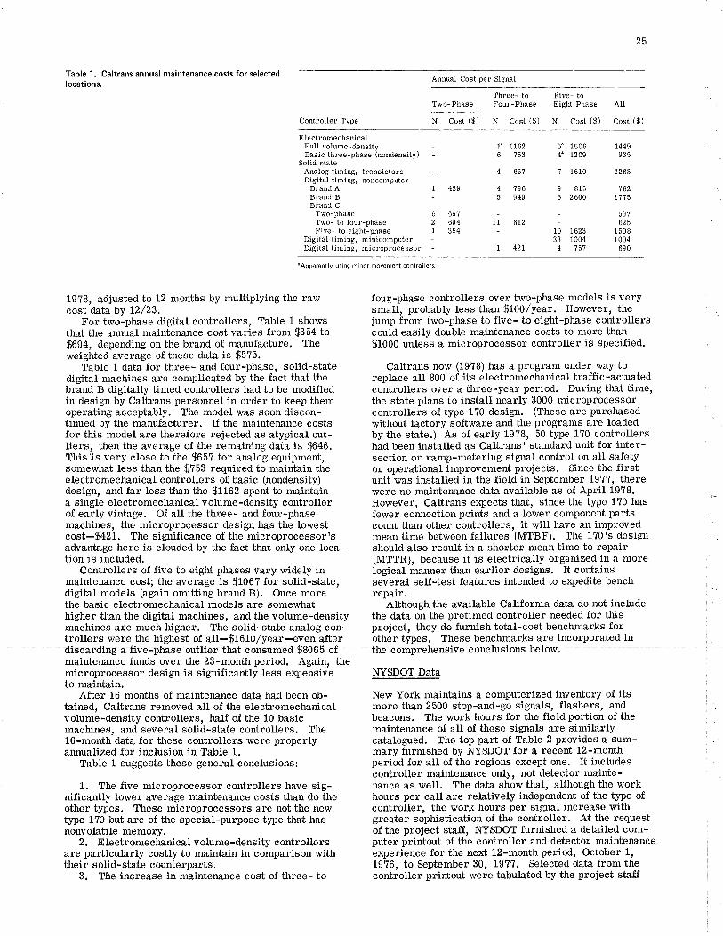
25
Table 1. Caltrans annual maintenance costs for selectedlocations.
Annual Cost per Signâl
Three- to Five- to
Controller Type N Cost ($) N cost ($) N cost ($) cost ($)
ElectromechanicalFull volume-densityBasic three-phase (nondensity)
Solid stateAnalog timing, transistorsDigitâl timing, noncomputer
Brand ABrand BBrand C
Two-phâselwo- to four-phaseFive- to eight-phase
Digitâl timing, minicompute¡Digital timing, microprocessor
7 429
1' 11626 753
4 65?
4 ?965 949
5' 1506 t4494' 1209 935
? 1610 1263
9 815 7825 2600 1??5
- 59?- 625
10 1623 1ã0833 1004 10044 75'.t 690
6 59?2 6941 354
tl 672
1 421
"Apparently using m¡nor movement controllers.
19?8, adjusted to 12 months by multiplying the rawcost data by t2/23.
For two-phase digital controllers, Table 1 showsthat the annual maintenance cost varies from $354 to$694, depending on the brand of manufacture. Theweighted average of these data is $5?5.
Table 1 data for three- and four-phase, solid-statedígital machines are complicated by the fact that thebrand B digitally timed controllers had to be modifiedin design by Caltrans persormel in order to keep themoperating acceptably. The model was soon discon-tinued by the manufacturer. If the maintenance costsfor this model are therefore rejected as atypical out-Iiers, then the average of the remaining data is $646.This'is very close to the $657 for an:alog equipment,somewhat less than the $753 required to maintain thee lectrome chanical c ontrolle rs of basic (nondensity)design, and far less than the $1162 spent to maintaina single electromechanical volume -derisity controlerof early vintage. Of all the three- and four-phasemachines, the microprocessor design has the lowest
tion is included.Controllers of five to eight phases vary widely in
maintenance cost; the average is $1067 for solid-state,
four-phase controllers over two-phase models is verysmall, probably less than $lOO/year. However, thejump from two-phase to five- to eight-phase controllerscould easily double maintenance costs to more than$1000 unless a microprocessor controller is specified. .
Caltrans now (1978) has a program under way toreplace atl 800 of its electromechanical tra-fÏic-actuatedcontrollers over a three-year period. During that time,the state plans to instatl nearly 3000 microprocessorcontrollers of type 1?0 design. (These are purchasedwithout factory sbftware and the programs are loadedby the state.) As of early 19?8, 50 type 1?0 controllershad been installed as Caltrans' standard unit for inter-section or ramp-metering signal control on all safetyor operational improvement projects. Since the firstunit was installed in the field in September 1977, therewere no maintenance data available as of April 1978.However, Caltrans expects that, since the
-ype 1?0 has
fewer con¡rection points and a lower component partscount than other controllers, it will have an improved
digibf models (again omitting brand B). Once more repair.the basic electromechanical models are somewhat Although the available California data do not insludehigher than the digital machines, and the volume-density the data on the pretimed controller needed for thismachines are much higher. The solid-state analog con- project, they do furnish total-cost benchmarks fortrollers were the highest of all-$1610/year-even after other types. These benchmarks are incorporated in
8O65 of tlte comprelænsì.ue conclusionsbeÏo-maintenance funds over the 23-montå period. Again, themicroprocessor design is significantly less expensiveto maintain.
After 16 months of maintenance data had been ob-tained, Caltrans removed all of the electromechanicalvolume-density controllers, haü of the 10 basicmachines, and several solid-state controllers. The16-month data for these controllers were properlyarurualized for inclusion in Table 1.
Table 1 suggests these general conclusions:
1. The five microprocessor controllers have sig-nificantly lower average maintenance costs than do theother types. These microprocessors are not the newtype 170 but are of the special-purpose type that hasnonvolatile memory.
2. E lectromechanical volume-density controllersare particularly costly to maintain in comparison withtheir solid-state counterparts.
3. The increase in maintenance cost of three- to
cost-$421. The significance of the microprocessor's mean time between failures (MTBF), The 170's designadvantage here is clouded by the fact that ònfy one loca- should also result in a shorter mean time to repair
(MTTR), because it is electricaUy organized Ín a morelogical manner than earlier designs. It containsseveral self-test features intended to er<pedite beneh
NYSDOT Data
New York maintains a computerized inventory of itsmore tlran 2500 stop-and-go signals, flashers, andbeacons. The work hours for the field portion of themaintenance of all of these signals are similarlycatalogued. The top part of Table 2 provides a sum-mary furnished by NYSDOT for a recent 12-monthperiod for all of the regions except one. It includescontroller maintenance only, not detector mainte-nance as well. The data show that, although the workhours per call are retatively independent of the type ofcontroller, the work hours per signal increase withgreater sophistication of the controller. At the requesfof the project staJf, NSSDOT furnished a detailed com-puter printout of the controller and detector mainter¡anceercperience for the next l2-month period, October 1,19?6, to September 30, 1977. Selected data from thecontroller printout were tabulated by the project staff
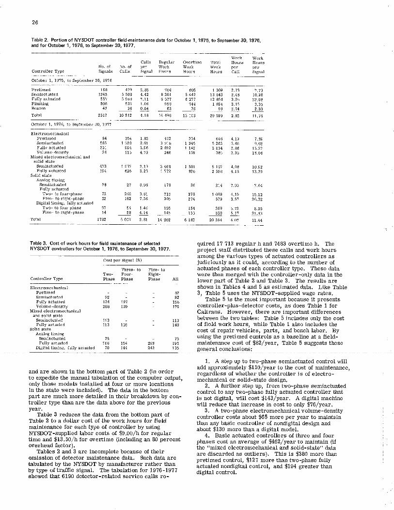
26
f able 2. Portion of NYSDOT controller field-maintenance data for October 1,1975, to September 30, 1976,and for October 1, 1976, to September 30, 1977 .
Controller Type
HoursperSignal
No. ofSignals
309300
20 384
CallsNo. of perCalls Signal
Regular Overtime Total HoursWork Work Work perHours Hours Hours Câll
October 1, 1975, to September 30, 19?6
PÌetimedSemiactuatedFully actuatedFlashingBeacon
Total
168 479 2.85 ',t041243 5 500 4.42 I 20155? 3 960 ?.11 6 5??506 53? 1.06 95043 36 0.84 63
25t',1 t0 5t2 4.18 16 496
1 309 2.73 7 .'1913 643 2.48 10.9812 854 3.25 23.081 694 3.15 3.35
99 2.74 2.30
29 599 2.82 11.76
6055 4426 z't',l
74436
13 103
October 1, 1976, to September 30, 19?7
ElectromechânicalPretimedSemiâctuatedFully actuatedVolume-density
Mixed electromechânicâl ândsolid state
SemiactuatedFully actuated
Solid stateAnalog timing
SemiactuatedFully actuated
TÞo- to four-phaseFive- to eight-phase
Digital timing, f ully actuatedTwo- to four phâseFive- to eight-phase
Total
154 1.83 4721520 2.61 3 918
994 3.96 2 692115 4.',t9 246
1 03? 2.19 3 666626 3.23 7 772
27 0.96 1?8
260 3.61 713162 ?.36 305
54 1.46 15558 4.t4 145
5 00? 2.87 14 202
4.t9 ?.693.46 9.033.86 75.2',13.35 16.04
4.98 10.924.1b 13.39
214 ?.93 7.64
1 089 4.19 15.725?9 3.57 26.32
84583251
24
473t94
7222
3?t4
1782
2341 3457 t42
139
1 501826
36
6465 2633 834
385
5 16?2 598
3?6274
154155
6 182
5.72 8.355.77 21.43
4.07 71.44
Controller Tjrpe
Table 3. Cost of work hours for field maintenance of selectedNYSDOT controllers for October 1,1976, to September 30,1977.
Cost per Signal ($)
quired 1? ?13 regular h and 7483 overtime h. Theproiect sta^tf distributed these calls and work hoursamong the various types of actuated controllers asjudiciously as it could, according to the number ofactuated phases of each controller type. These datawere then merged with the controller-only data in thelower part of Table 2 and Table 3. The results areshown in Taþles 4 and 5 as estirnated data. Like Table3, Table 5 uses the NYSDOT-supplied wage rates.
Table 5 ís the most important because it presentscontroller-plus-detector costs, as does Table 1 forCaltrans. However, there are important differencesbetween the two tables: Table 5 includes only the costof field work hours, while Table 1 also includes thecost of repair vehicles, parts, and bench labor. Byusing the pretimed controls as a baseline at a field-maintenance cost of fiïZ/year, TaþIe 5 suggests thesegeneral conclusions:
Two-Phase
Three- to Five- toFour- Eight-Phase Phase AII
Elect¡omechanicalPretimedSemiactuatedFully actuatedVolume-density
Mixed electromechanicaland solid state
SemiâctuatedFully actuated
Solid stateAnalog timing
SemiactuatedFully actuated
Digital timing, fully actuated
-82-92- 158- 1?0
- 113_ 140
-?5293 191243 135
ni-134 19?208 109
113113 155
75166 15410 144
and are shown in the bottom part of Table 2 (in orderto e4pedite the manual tabulation of the computer output,only those models installed at four or more locationsin the state were included). The data in the bottompart are much more detailed in their breakdown by con-troller type than are the data above for tl¡e previousyear.
Table 3 reduces the data from the bottom part ofTable 2 to a dollar cost of the work hours for fieldmaintenance for each t¡pe of controller by usingNYSDOT-supplied labor costs of $9.00/h for regulartime and $13,50/h for overtime (including an 80 percentoverhead factor).
Tab1es 2 and 3 are incomplete because of theiromission of detector maintenance data. S.rch data aretabulated by the NIISDOT by manufacturer ratber t¡anby type oftra-ffic signal. The tabulation for 19?6-197?showed that 6190 detector-related service calls re-
1. A step up to two-phase semiactuated control u¡illadd approximately $110/year to the cost of maintenance,regardless of whether the controller is of electro-mechanical or solid-state design.
2. A further step up, from two-phase semiactuatedcontrol to any two-phase fully actuated controller tl¡atis not digital, will cost $143/year. A digital machinervill reduce that increase in cost to only fi76/year.
3. A two-phase electromechanical volume -densitycontroller costs about $65 more per year to maintainthan any basic controller of nondigital design andabout $130 more th¿ü a digital model.
4. Basic actuated controllers of three and fourphases cost an average of.fi462/year to maintain (ifthe "mixed electromechanical and solid-state" dataare discarded as outliers). This is $380 more thanpretimed control, $12? more than two-phase fullyactuated nondigital control, and $194 greater thandigiial control.
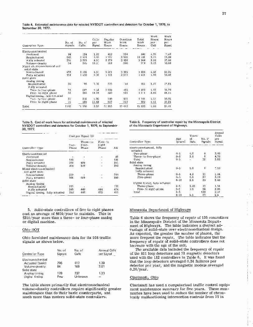
27
Table4. Est¡matedma¡ntenancedataforselectedNYSDOTcontrollersanddetectorsforOctoberl,19T6,toSeptember 30,1977.
Controller TypeNo. ofSignals
CallsperSignal
No. ofCâl1s
Regular Overtime TotaÌ Hours HoursWork Work Work per perHours Hours Hours CaU Signal
ElectromechânicalPretimedSemiactuatedFully âctuatedVolume-density
Mixed electromechanical andsolid state
SemiactuatedFully actuated
Solid stateAnalog timing
SemiactuatedFuIIy actuated
Two- to four-phaseFive- to eight-phase
Digital timing, fully actuâtedTwo- to four-phaseFive- to eight-phase
Total
154 1.83 4t22 874 4.93 '.t 7972 385 9.51 6 6?8
246 10.21 618
646 4.19 7.6910 ?81 3.?5 18.49I 504 3.98 37.86
914 3.73 38.08
9 626 4.52 20.357 461 4.10 38.46
491 5.77 7'.t .54
2 829 4.12 39.291 411 3.86 64.t4
7 741 4.47 30.84829 4.4t 59.21
45 633 4.08 25.61
84583251
24
473t94
6 8015 191
2 7321 820
2342 9842 826
296
2 8252 270
373 118
1 936 893890 621
28 95
't2 68722 366
4.519.39
3.39
9.541 6.64
JI
74
t782
401312
13 680
259 ?.00 740188 13.43 51?
11 190 6.28 31 953
Table 5. Cost of work hours for estimated ma¡ntenance of selectdNYSDOT controllers and detectors for October 1, 1976, to September30,1977.
Cost per Signal ($)
Controller Type
Three- to Five- toTwo- Four- Eight-Phâse Phase Phase
Table 6. Frequency of controller repair by the Minneapol¡s Districtof the Minnesota Department of Highways.
Controller Type
AnnualYears CâUs
Age of No. of per(years) Data signals Signâl
All
ElectromechanicalPretimedSemiâctuatedFully actuatedVoIume-density
Mixed electromechanicaland solid state
SemiactuatedFully actuated
Solid stateAnalog timing
S€miactuatedFully actuated
Digital timing, fully actuated
-82- 189- 391- 398
_ 210- 399
- 117684 4',t4633 411
Electromechanical, f ullyactuated
Two-phaseThree- to five-phâseTotaI
Solid stateAnalog timing
SemiactuatedFully actuated
Three-phaseFive-phase
Digital timing, fully âctuatedThree-phaseFive- to eight-phase
Totâl
3.45 13 1.343.0 24 2.05- 100 2.3't2.5 23 2.4
0-5 5.0 I0-5 3.0 40-5 - 72
5.0
4.95.02.5
2.404.702.92189
330398
270309
717365268
4S;398
44;448
619
0-5
0-50-56- 10
0-50-5u-b6- 10
2 7.70
11 1.84z'.î 3.1923 2.40
Ohio DOT
Ohio furnished maintenarce data for its 558 tra-fficsignals as showlr below.
5. Solid-state controllers of five to eight phasescost ¿ur average of $659/year to maintai.n. This isfiZL}/year more than a three- or four-phase analogor digital machine.
Minnesota Department of Highways
Table 6 shows the frequency of repair of 135 controllersin the Minneapolis District of the Minnesota Depart-ment-of llighways. The-Jablejndicates a-distinct ad-vantage of solid-state over electromechanical design'As expected, the greater the number of phases, themore frequent the repair, The table indicates t¡at thefrequency of repair of solid-state controllers does notincrease with the age of the unit.
The available data included the frequency of repairof the 811 loop detectors and 12 magnetic detectorsused with the 112 controllers in Table 6. It was foundthat the loop detectors averaged 0.24 failures perdetector per year, and the magnetic models averagedQ.26/year.
Cincinnati, Ohio
Cincirurati has used a computerized tra-flic control equip-ment maintenance sumrnary for five years. These sum-maries have been used to reduce the number of chron-ically malfunctíoning intersection controls from 17 in
No. of No. ofController Type Signals Calls
E lectromechanicalActuated (basic)Volume-density
Solid stateAnalog timingDigital timing
296 412 1.3984 169 2.O1
178Few
237Unknown
Annual Callsper Signal
1.33
The table shows primarily tùat electromechanicalvolume -density controllers require significantly greatermaintena¡ce than do their basic cowrterparts, andmuch more than modern solid-state controllers.
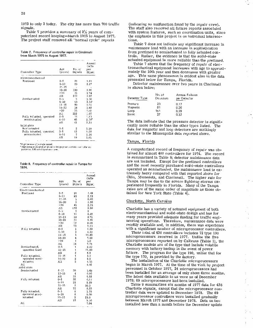
28
1973 to only 2 today. The city has more than 700 tra-fficsignals.
Tabte ? provides a sumrnary ot 2L/2 yearc of com-
The project staff removed all "normal cycle" reports
Table 7. Frequency of controller repair in Cincinnatifrom March 1975 to August 1977.
Controller Type
AnnualCaIls
Age No. of per(years) Signals Signal
ElectromechanicalPretimed
(indicating no malfunction found by the repair crew),The sta-ff also removed all failure reports associatedwith system features, such as coordination units, since
tions.Table 7 does not indicate any significant increase in
rnainteriance load with an increase in sophisticationfrom pretimed to semiactuated to fully actuated con-trols. Rather, the evidence is that the solid-stateactuated equipment is more reliable than the pretimed.
Table 7 shows that the frequency of repair of elec-tromechanical equipment increases with age to approxi-mately the 10th year and then decreases with greaterage. This same phenomenon is evident also in the datapresented below for Tampa, Ftorida.
Detector maintenance over two years in Cincinr¡atiis shown below:
0-56- 1011- 1516-20>20All0-56-1011- 1516-20>20Au0-56- 10AII
0-50-56- 10AII
1.812.t'l
1.99t.7 47.921.502.5tL701.651.681.8?1.132.7 60
1.501.001.t41.05
No. ofDetectors
31Jâ
trã72
2'Ì't2
48805438
222164561
272
19
Detector Type
PressureMagneticLoopSonic
Annual Failuresper DetectorSemiactuated
FuÌl.y actuated, operatedsemiâctuated
Solid stateSemiactuatedFully actuated, operâted
semiactuâted
23 0.178f 0.26151 0.2937 0.32
ControÌ.ler TypeAge No, of(years) signals
" H igh becâuse of a s¡ngle model.bHigh because 20 un¡ts of an early-d6ign phase,modular controller ex,
per¡enced 3.85 calls/signal eâch year.
Table 8. Frequencyof controller repair in Tampa for1974.
The data indicate that the pressure detector is signifi-cantly more reliable than the other types Listed. Thedata for rnagnetic and loop detectors are strikinglysimilar to the Mirureapolis data reported above.
Tampa, Florida
A computerized record of frequency of repair was ob-tained for almost 400 controllers for 1g?4. The recordis summarized in Table 8; detector maintena.nce dataare not included. Except for the pretimed controllersand the most recently purchased solid-state controllersoperated as semiactuated, the maintenance load is ex-tremely heavy compared'¡¡ith that reported above forOhio, Minnesota, and Cincinnati. The higher rate forTampa may be due to the severe lightning storms ex-perienced frequently in Florida. Many of the Tamparates are of the same order of magnitude as those ob-tained for New York State (Table 4).
Charlotte. North Carolina
Charlotte has a variety of actuated equipment of bothelectromechanical and sotid-state design and has formany years provided adequate funding for traffic engi-neering operations. Therefore, maintenance data were
Their total of 438 controllers includes ?2 type 190microprocessors received in 19TT. Unlike the fivemjcroprocessors reported on by Caltrans (Table 1), theCharlotte models are of the type that include volatilememory witlt battery backup in the event of powerfaÍlure. The program for the type 190, unlike that forthe type 170, is provided by the factory.
The inst¿llation of the Charlotte microprocessorsbegan in March 19??. At the time of tire visit by projectpersonnel in October L977, 24 microprocessors hadbeen installed for an average of only about three months.
'The latest data availa.ble to us '!¡/ere as of December1978; 69 microprocessors had been installed. l
Table I summarizes six months of 19TT data for 4BBCharlotte signals, except that the microprocessor con-troller clata were updated to December 1g?8. The 6gmicroprocessor controllers were installed gradually ]
between March 197? and December 19?8. Data on twoinstalled less tha¡ a month before the December update
AmualCallsperSignal
ElectromechanicalPretimed 0-5 32
6-10 9311- 15 516-20 1>20 45All 1?60-5 1
6-10 111t-15 3816-20 11
6- 1011- 1516-20>20
1.692.330.401.002.762.2606.828.? 1
4.46>20 t2 9.08 - ,., " : -.,:,-_,---'Âu 1j j-tr rea¿tty avatta¡te anC
Fully actuated 0-5 1 1.00 with a significant number of microprocessor controllers.
Semiactuated
Semiactuated,operâted fixed
Fully actuated,operated semi-actuated
AllSolid state
Semiâctuâted
Ful.ly âctuated
Fully actuated,operated semi-actuated
All
AÌ10-511-15All11- 1516-20All
6- 1011- 15AII0-56-1011- 15All0-56- 1011- 15Alt
4.33I 1.807.505.0,t.71
2.0011,00
6.53.05.04.3 34.09
5.486.005.5 5
6.1?9.09
30.08.237.755.00
23.05.56't.04
l4I1t1
2
294
óó35
2?0I82
18
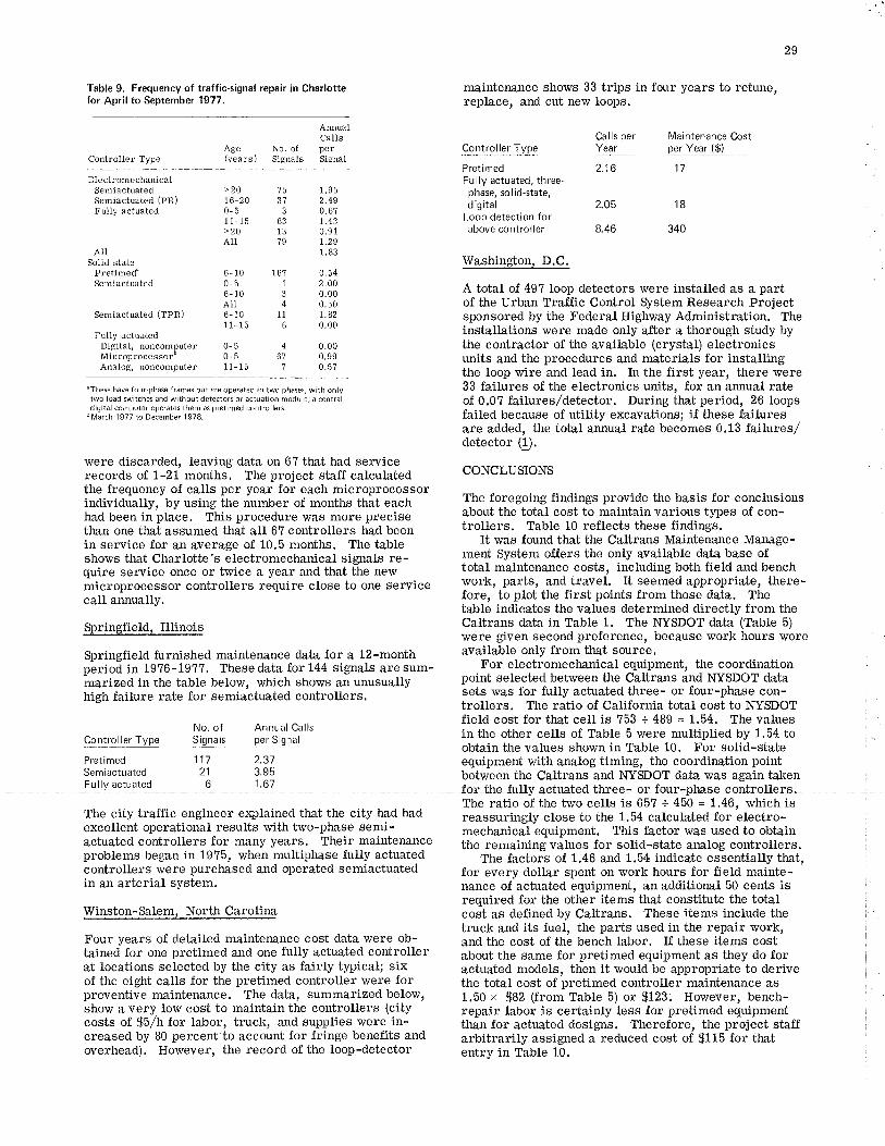
29
Table 9. Frequency of traffic-signal repair in Charlottefor April to September 1977.
Controller Type
ArnrualCalls
Age No. of per(years) Signals Signal
maintenance shows 33 trips in four years to retune,repÞce, and cut new loops.
Controller TypeCalls per Maintenance CostYear per Year ($)
Pretimed 2.16Fu lly actuated, three-
phase, solid-state,digital 2.O5
Loop detection forabove controller
Washington, D.C.
1.9 5
2.490.671.430.917.291.83
0.542.000.000.501.820.00
8.46
17
18
340
ElectromechanicalSemiâctuatedSemiactuated (PR)Fully actuâted
AllSolid state
P¡etimed'Semiactuated
semiactuâted (TPF)
Fully actuatedDigital, noncomputerMic rop roce sso r"Analog, noncomputer
>2016-200-511- 15>20AIl
6- 100-56- 10All6- 1011- 15
0-50-511- 15
75
J
bJ
?9
16?1
34
11b
467
6_10 3 0.00 A total of 497 loop detectors were installed as a part
semiactuâted (rp*) å]i, 1l Î:å9 0f the urban Traffic control system Research Project
Fu"y ac,ua,ed 11-15 6 o o0 itrHå1i:#Jli"ixi::iir"HH *tni;:!il$ä; i,l"Disital, noncomputer 0-b 4 0.00 the contractor of the available (crystal) electronicsMicroprocessor" 0-5 67 0.99 units and the proCedures and materials for installingAnalos' noncomputer 11-15 ? 0 57 the loop wire and lead in. I¡r the first year, there were
.Theæ have foutrphas frames but are operated ¡n lwo phases. wìth onty 33 failures of the electronics units, for an arurual raterwoloadswitchesandwirhourderecrorsoractuarionmodute;acentrat Of 0.0? failUfeSr/deteCtOf. DUfing that pefiOd, 26 IOOpSdigital computer operates them as pretimed controllers.
brvarch re77 to Dæember 1e78. failed because of utility excavations; if these failuresare added, the total amual rate becomes 0.13 failures/detector Q.
were discarded, leaving data on 6? that had servicerecords of 1-21 monthsl The project staff calculated coNcLUsIoNSthe frequency of calls per year for each microprocessorindivid,ally, by using ihe number of months iËt;;th - The foregoing findings provide the basis for conclusions
had been inþface. This procedure was r"o"u p"uàiÀã 3Uo¡t the total cost to maintain various types of con-
than one that assumed that all 6? controller" fñ¿ ¡ã"n trollers. Table 10 reflects these findings.in seryice for an average of 10.5 months. The table It was found that the caltrans Maintenance Manage-
shows that Charlotte's ðlectromechanicat signats'rã- ment System offers the only available database ofquire service once or twice a year a¡rd that tire-ne* total maintenance costs, including both field and bench
iri""op"oc".sor controllers réquire close to one service work, parts, and travel. It seemed appropriate, there-call annually {o19, .to plot the first points from those data. The
table indicates the values determined directly from the
Sþringfield. Illinois Caltrans data in Table 1. The NYSDOT data (Table ã)were given second preference, because work hours were
Springfield furnished maintenance data for a 12-month available only from that source'
ññã in-is?6-t9zz. These data for 144 signats are sum- .For electromechanical equþment, tre coordinationmarized in the table below, rvhich shows an unusually point selected between the Caltrans and NYSDOT data
high failure rate for semiactuated controllers. sets- was for fully actuated three- or four-phase con-trollers. The ratio of California total cost to NYSDOT
No. of Annuat ca's field cost for that cell is 753 + 489 = L.64. The values
ggqlgllgflylg sisnals persisnal in the other cells of Table 5 were multiplied by 1'54 toobtain the values shown in Table 10. For solid-state
Pretimed 117 2.37 equipment with analog timing, the coordination pointsemiactuated 21 3'95 between the Caltrans and NYÐOT data was again talenFully actuated 6 1.67 tor the f'
The city traffic engineer explained that the city had hadexcellent operational results with two-phase semi-actuated controllers for many years. Their maintenanceproblems began in 1975, when multiphase fully actuatedcontrollers were purchased and operated semiactuatedin an arterial system.
'Winston-Salem. North Carolina
Four years of detailed maintenance cost data lvere ob-tained for one pretimed and one fully actuated controllerat locations selected by the city as fairly typical; sixof the eight calls for the pretimed controller were forpreventive maintenance. The data, summarized below,show a very low cost to maintain the controllers (citycosts of $5/h for labor, truck, and supplies were in-creased by B0 percent to account for fringe benefits andoverhead). However, the record of the loop-detector
The ratio of the two cells is 657 + 450 = 1.46, which isreassuringly close to the 1.54 calculated for electro-mechanical equipment. This factor was used to obtainthe remaining values for solid-state analog controllers.
The factors of 1.46 and 1.54 indicate essentially that,for every dollar spent on work hours for field mainte-nance of actuated equipment, an additional 50 cents isrequired for the other items that constitute the totalcost as defined by Caltrans. These items include thetruck and its fuel, the parts used in the repair work,and the cost of the bench labor. If these items costabout the same for pretimed equipment as they do foractuated models, then it would be appropriate to derivethe total cost of pretimed controller maintenance as1.50 x $82 (from Table 5) or $123: However, bench-repair labor is certainly less for pretimed equipmentthan for actuated designs. Therefore, the project sta"ffarbitrarily assigned a reduced cost of $115 for thatentry in Table 10.
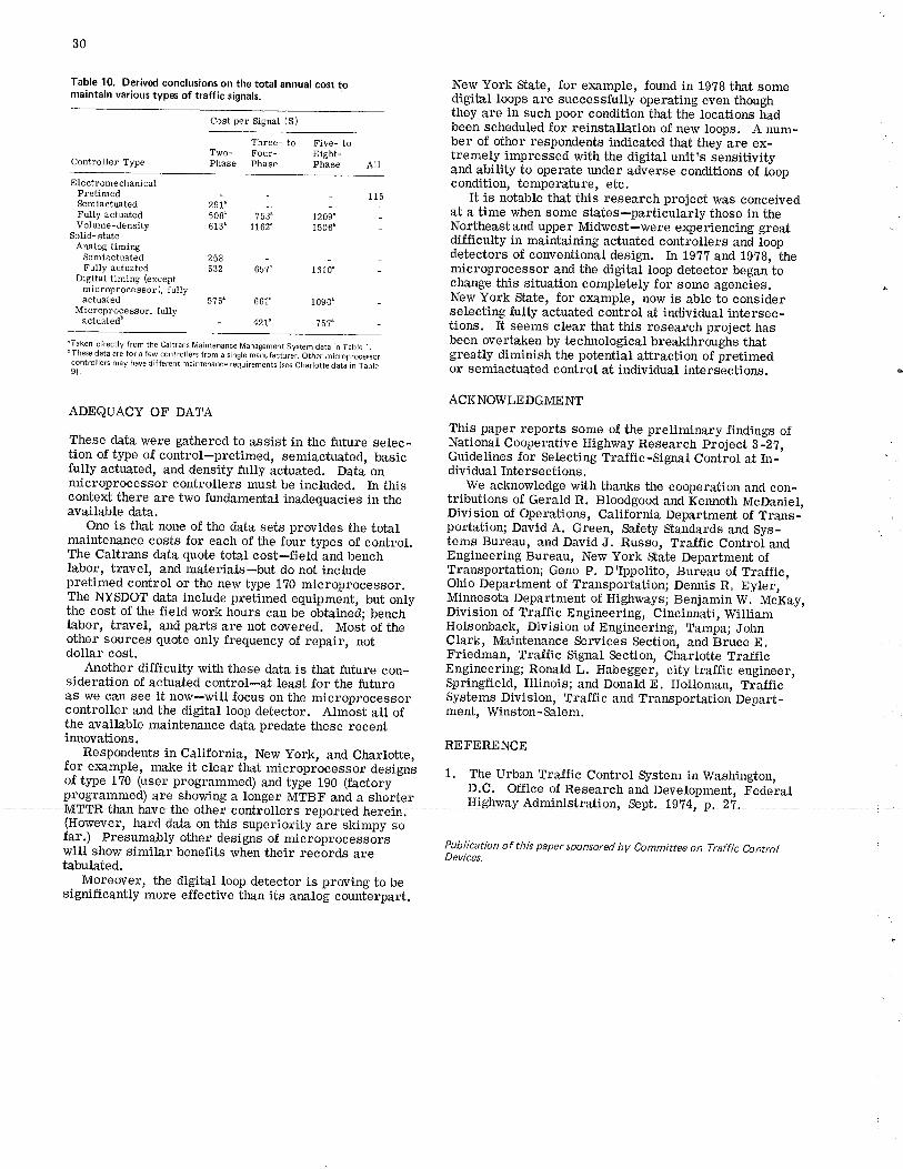
Cost per Signal ($)""-. "", ",".,-r r*
30
Table 10. Derived conclusions on the total annual cost toma¡nta¡n various types of traffic signals.
New York Süate, for example, found in 19?B that somedigitat loops are successfully operating even thoughthey are in such poor condition tj¡at the locations had
þer of other respondents indicated that they are ex-tremely impressed with the digital unit,s sensitivityand abi[ty to operate under adverse conditions of loopcondition, temperature, etc.
It is notable that this research project was conceivedat a time when some states-particularly those in theNortheast and upper Midwest-were e4periencing greatdifficulty in maintaining actuated controllers and loopdetectors of conventional design. h 19?? and 19T8, themicroprocessor and the digitat loop detector began tochange this situation completely for some agencies.New York State, for e:ømple, now is able to considerselecting fully actuated control at individual intersec-tions. It seems clear that this research project hasbeen overtaken by technological breakthroughs thatgreatly diminish the potentiat attraction of pretimedor semiactuated control at individual intersections.
ACKNO\ryLEDGMEI{I
This paper reports some of the preliminary findings ofNational Cooperative Highway Research project B-2?,Guidelines for Selecting Traffic-Signal Control at In-'dividual Intersections.
'We acknowledge with thanks the cooperation and con-tributions of Gerald R. Bloodgood and Kenneth McDaniel,Division of Operations, California Department of Trans-portation; David A. Green, Safety Standards and Sys-tems Bureau, and David J. Russo, Tra^tfic Control andEngineering Bureau, New York Sate Department ofTransportation; Geno P. Drlppotito, Bureau of Traflic,Ohio Department of Transportation; Dennis R. Eyler,
-
Minnesota Department of Highways; Benjamin W. McKay,Division of Tra-ffic Engineering, CincÍrurati, WilliamHolsonback, Division of Engineering, Tampa; JohnClark, Maintenance Services Section, and Bruce E.Friedman, Tra^ffic Signal Section, Charlotte Tra-fficEngineering; Ronald L. Habegger, city traffic engineer,Springfield, Illinois; and Donald E. Holloman, TrafficSystems Division, Tra-ffic and Transportation Depart-ment, Winston-Salem.
REFERENCE
1. TheD.C.
Urban Tra-tfic Control System in Washington,Office of Research and Development, Federal
1
Controller Type
Three- to Five- toTwo- Four- Eight-Phase Phase Phase All
ElectromechanicalPretimedSemiactuatedFully âctuatedVolume-density
Solid- stateAnalog timing
SemiactuâtedFully âctuâted
Digital timing (exceptmicroprocessor), fullyactuated
Microprocessor, fullyâctuâtêdò
zsì"50tr613'
258
zsã:1162'
65?'
-1209'1506'
161 0'
1090"
757^
tt:
5?5' 661"
_ 427'
'Taken directly from the Caltrans Maintenance lvlanagementsystem data ¡n Table l_bTheæ data are for a lew controllers from a single ma-nutactuidr. ätt ai.i"rop,o"u*o,controllers may have d¡fferent ma¡ntenance requirements (se Charlotte data in Table
ADEQUACY OF DATA
These data were gathered to assist in Ûre future selec-tion of type of control-pretimed, semiactuated, basicfully actuated, and density fully actuated. Data onmicroprocessor controllers must be included. I¡r thiscontext there are trvo fundamental inadequacies in theavailable data.
One is that none of the data sets provides the totatmaintenance costs for each of the four types of control.The Caltra¡rs data quote total cost-field and benchlabor, travel, and materials-but do not includepretimed control or the new type 1?0 microprocessor.The NYSDOT data include pretimed equipment, but onlythe cost of the field work hours can be obtained; benchlabor, travel, and parts are not covered. Most of theother sources quote only frequency of repair, notdollar cost.
A¡other difficulty with these data is tt¡,at future con-sideration of actuated control-at least for the futureas vr'e can see it now-will focus on the microprocessorcontroller and the digital loop detector. Almõst all ofthe available maintenance data predate these recentinnovations.
Respondents in California, New york, and Charlotte,for example, make it clear that microprocessor designsof type 170 (user programmed) and type 190 (factoryprogrammed) are showing a longer MTBF and a shorter
will show similar benefits when their records are
, P' 27'(However, hard data on this superiority áre skimpy sofar.) Presumably other designs of microprocessors
tabulated.Moreover, the digital loop detector is prwing to be
significantly more effective than its analog counterpart.
Publication of th¡s paper sponsored by Committee on Traffic ControlDevices.
31
Reflecto rization of Railroad Rolling StockRichard G. McGinnis, Department of Civil Engineering, Bucknell University, Lewisburg,
Permsylvania
This paper examines the effectiveness of retroreflectors on the s¡des ofrailroad rolling stock as a means of reducing highway-railroad grade-crossing accidents, and it estimates the benefits and costs of reflec-torizing the U.S. fleet of railroad cars. Factors that affect the amountof reflected light received by a driver (including reflector characteris-tics, vehicle-reflector positioning, reflector cleanliness, headlight clean-liness and beam usaç, windsh¡eld transm¡ttance, and atmospheric con-ditions) were analyzed, and expected reflector illuminance levels wereprcd¡cted. Under conditions expected in railroad operat¡on, the analys¡s¡nd¡cates that 15cm (6-in) square delineators of high-intensity-grade re-flective sheeting will permit detect¡on d¡stances sufficient for safe stop-ping in most highway s¡tuat¡ons, even under low-beam headlight illumina-tion. Benefits were estimated from the 1975 Federal Railroad Ad-ministration accident data. Acc¡dents were categorized into four groupsbased on the speeds of the train and motor vehicle and the collisionpoint on the train. Reflector effectiveness for each of these groups wasestimated by considering the type of crossing warning device, daylightacc¡dent rates, weather cond¡tions. presence of obstruct¡ons, human fac-tors associatd with nighttime driving, and the train and motor vehicleçeeds. The costs of a reflectorization program were estímated and aoost+ffect¡veness analysis was performed to assess the impact of v¡si-bility at grade crossings on annual benefits, since no reliable informa-tion is available on this important factor.
Conflicts between trains and automobiles at highway-railroad grade crossings have long been recognized asa major safety problem. Since the 1920s, the railroadsand various local, state, and federal government agen-cies have worked to reduce hazards at the 220 000 publicgrade crossings in the United States.
Statistics indicate that efïorts to improve the safetyat grade crossings have been effective: in 1928 therewere 2568 fatalities resulting from grade-crossingaccidents (!); in 19?7, this figure was 63 percent lower,even though vehicle kilometers of travel increased morethan 800 percent during the same period Q).
Unfortunately, the problem of grade-crossing acci-dents has still not been completely solved. There weremore than 12 000 grade-crossing accidents reported tothe Federal Railroad Administration (FRA) in 1977.Consequently, FRA and the Federal Highway Administra-tion are continuíng their programs to reduce the hazardsof railroad-highway grade crossings.
Most grade-crossing sa-fety programs have beeni$red atimproving
crossing, but another approach is to improve the con-spicuity of the train, so that motorists can actuallydetect it near a crossing. At some crossings, for ex-ample, street lights Ìrave been installed to improvenighttime visibility. On-train devices have also beenproposed. Recently, interest has been high in the useof strobe lights on locomotives to Ímprove both dayand nighttime train visibility. Also, the use of reflec-tors on the sides of railroad cars has long been ad-vanced by some as an effective way of increasing night-time train visibility.
The purpose of this study was to examine the efïec-tiveness of reflectors on the sides of railroad cars asa means of reducing grade-crossing accidents. Theuse of reflectors on railroad cars has been discussedin many documented studies (!q-Ð, but the conclusionsreached in these investigations are not consistent andindicate that the effectiveness of reflectors in reducinggrade-crossing accidents may be either very con-siderable or absolutely minimal. This paper provides
both an in-depth analysis of reflector effectiveness andan exa,mination of the benefits and costs of reflectoriz-ing the sides of the U.S. railroad car fleet.
REFLECTORIZATION
Reflectorization has its greatest sa-fety potential foraccidents that occur at nigirt and irwolve a motor vehiclestriking the side of a train. In many of these accidents,the motorist is apparently unable to see the train intime to stop the vehicle saJely. Reflectors on the sideof a railcar rvill reflect Light from a motor vehiclersheadlights back toward tlte vehicle and, to the driver,such reflectors will appear as light sources or "brightspots" against a dark background.
The approach t¿ken to analyze the effectiveness ofreflectorization was to examine first the factors tÀata^ffect the amount of reflected light that can be erçectedat various distances from a grade crossing and then tocompare these light levels witlt visual detection stan- .
dards to see whether detection (and perception) of atrainrs presence is likely.
The type of reflector that wor¡ld be used on railroadcars is called a retroreflector or reflexreflector.Retroreflectors reflect incident light back toward thelight source in a narrow beam. Retroreflective ma-terials are used extensively for highway signs, pave-ment markings, and motor vehicle markings.
The amount of light received by an observer from aretroreflector is a-tTected by six factors: the reflectiveintensity of the reflector, its size, the intensity of theoriginal light source, atmospheric transmissivity,windshield transmittance, and its distance from theobserver. The relationship between these factors andillumina¡ce received by the observer is given by Equa-tion 1:
L=(t.ARt2dw)/d4
where
Eo=Is=
illuminance received by the observerintensity of the light beam toward the
(1)
(lx),reflector
ARt
wd
areá of the reflector (m2),ref Ie ctiv e intensity of
'
the' ref le ct or l(cd / lÐ / rrt l,= transmissivity of the atmosphere per meter,= rvindshield transmittance, and= distance between the obseryer and the reflector
(m).
A FORTRAN computer program was written to com-pute reflector illumina¡ce received by a driver forvarious reflector (train) locations. The program usedheadÞmp luminous -intensity distributions and retrore-flector properties to determine expected reflectorbrightness. Values were computed for reflector loca-tions from 30 m (100 ft.) to 244 m (800 ft) in front of themotor vehicle and from 122 m (400 ft) to the left to122 mto the right of the projected path of the motorvehicle. tr addition, the program allowed for variationin the size, efficiency, and placement height of reflec-tors; the conditions of headlights, windshields, and
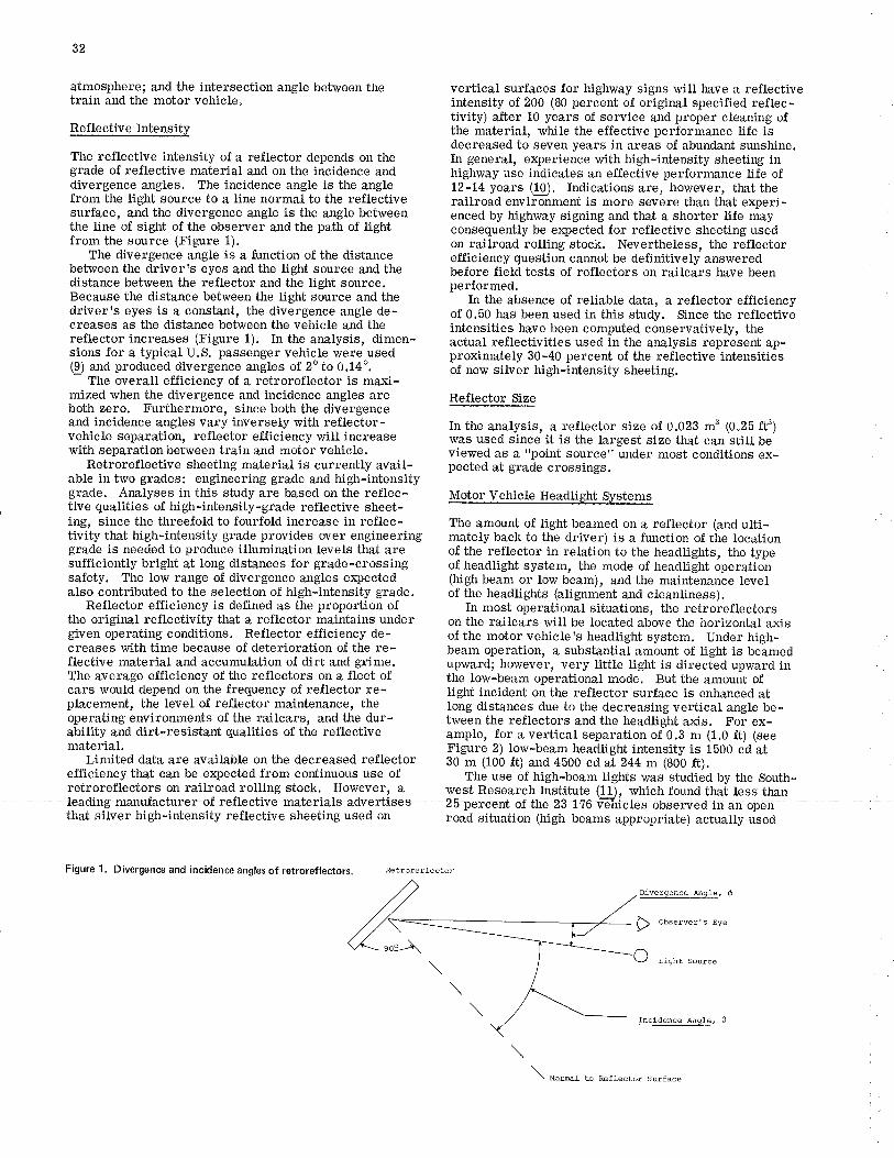
tivity that high-intensity grade provides over engineering mately back to the driver) is a function of the locationgrade is needed to produce illumination levels that are of the reflector in relation to the headlights, the typesufficiently bright at long distances for grade-crossing of headlight system, the mode of headlight óperationsafety. The low range of divergence angles e¡pected (high beam or lorv beam), a¡d the mainténance levelalso contributed to the selection of high-intensity grade. of the headlights (atignment a¡rd cleanliness).
Reflector efliciency is defined as the proportion of In most operational situations, the retroreflectorsthe original reflectivity that a reflector maintains under on the railcars will be located above the horizontal axisgiven operating conditions. Reflector efficiency de- of the motor vehiclers headlight system. Under high-creases with time because of deterioration of the re- beam operation, a sulrstantial amôunt of light is beãmedflective material and accumulation of dirt and grime. upward; however, very litge light is direcled upward inThe average efliciency of the reflectors on a fleet of the low-beam opérational mode. But the amo'nt ofcars would depend on the frequency of reflector re- üght incident oñ the reflector surface is enha¡rced atplacement, the level of reflector maintenance, the tong distances due to the decreasing vertical angle be-operating environments of the railcars, and the dur- tween the reflectors and the headfifht axis. For ex-ability and dirt-resistant qualities of the reflective ample, for a vertical separation ofg.B * (1.0 ft) (seematerial. Figure 2) low-beam headlight intensity is i5oo cO at
Limited data are available on the decreased reflector 30 m (10b ft) and 4500 cd {t Z++ m (g¡b ft).efficiency that can be e4pected from continuous use of The use óf nigh-neam lights was stu¿iéO Uy the South-retroreflectors on railroad rolling stock. However, a west Research Institute (11j, which found thai less thanfcading-rn'anufaeturerofrreflestive materials adçertises ?Spc¡ecnt of ¡re23 126 vre'eÉÍaOSOnrythat silver high-intensity reflective sheeting used on road situation (high beams appropriate) actually uied
32
atmosphere; and the intersection angle between thetrain and the motor vehicle"
Reflective Intensity
The reflective intensity of a reflector depends on thegrade of reflective material and on the incidence anddivergence angles. The incidence angle is the anglefrom the light source to a line normal to the reflectivesurface, and the divergence angle is the angle betweenthe tine of sight of the observer and the path of lightfrom the source (Figure 1).
The divergence angle is a function of the distancebetween the driver's eyes and tlte light source and thedistance between the reflector and the light source.Because the distance between the light sourse and thedriveris eyes is a constant, the divergence angle de-creases as the distance between the vehicle and thereflector increases (Figure 1). In the analysis, dimen-sions for a typical U.S. passenger vehicle were used(p) attd produced divergence angles of 2o to 0.14o.
The overall efïiciency of a retroreflector is maxi-mized when the divergence and incidence angles areboth zero. Furthermore, since both the divergenceand incidence angles vary inversely with reflector-vehicle separation, reflector efficiency rvill increasewith separation between train and motor vehicle.
Retroreflective sheeting material is currently avail-able in two grades: engineering grade and high-intensitygrade. Analyses in this study are based on the reflec-tive qualities of high-intensity-grade reflective sheet-ing, since the threefold to fourfold increase in reflec-
Figure 1. Divergence and incidence angles of retroreflectors. Retrorerrcc:o'
vertical surfaces for highway signs will have a reflectiveintensity of 200 (80 percent of origin:al specified reflec-tivity) after 10 years of service ard proper cleaning ofthe material, while tlte eflective performance life isdecreased to seven years in areas of abundant sunshine.fn general, experience with high-intensity sheeting inhighway use indicates an effective performance life of12-14 years (10). Indications are, however, that therailroad environment is more severe than that experi-enced by highway signing and that a shorter life mayconsequently be expected for reflective sheeting usedon railroad rolling stock. Nevertheless, the reflectorefficiency question cannot be definitively answeredbefore field tests of reflectors on railcars have beenperformed.
ln the absence of reliable data, a reflector efficiencyof 0.50 has been used in this study. Since the reflectiveintensities have been computed conservatively, theactual reflectivities used in tJre aaalysis represent ap-proximately 30-40 percent of the reflective intensitiesof new silver high-intensity sheeting,
Reflector Size
In the analysis, a reflector size of 0.023 m' 1O.ZS tt'¡was used since it is the largest size that can still beviewed as a "point source" under most conditions ex-pected at grade crossings.
Motor Vehicle Headlight Systems
The amount of tight beamed on a reflector (and ulti-
Divergence hgle, 0
\ observer's Eye
Light Source
Incidence hg1e, 0
\ to.*t Lo RefÌector suface
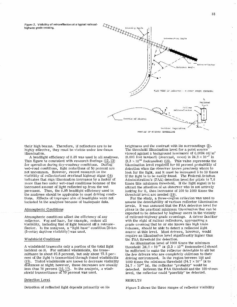
33
Retroreflecto¡Entrance hgle
PN VIEW OF MILROAD - HTGH}IAY G¡ÀM CROSSING
brightness and the contrast with its surroundings Q).The threshold illumination level for a point sourceviewed against a background luminance of 0.0034 cd/rn'z(0.001 foot lambert) (overcast, moon) is 24.? x 10-'g Ix(2.3 x 10⁴ footcandles) (19. This value represents theillumin:ation level requirèd for 98 percent probability ofdetection when the observer knows precisely where tolook for the light, and it must be increased 5 to 10 timesif the light is to be easily found. The Federal AviationAdministration's (FAA) detection level for pilots is ?.8times this minimum threshold. If the light signal is toattract the attention of an observer who is not activelylooking for it, then increases of 100 to 1000 times thethreshold level are needed (19).
For the study, a three-region criterion was used toassess the deteclability of various reflector illuminationlevels. It was assumed that the FAA detection level for
"*p""þrdlP" b+ä:lå:?HËffiåil,";iHHi"1'ffiH*?iff +
Figure 2. Visibility of retroreflectors at a typical railroad-highway grade crossing.
their high beams. Therefore, if reflectors are to behighly effective, they must be visible under low-beamillumination.
A headtight efficiency of 0.85 was used in all analyses.This figure is consistent with research findings (¡4!!)for operation during dry-roadway conditions. Duringwet-road conditions, light reductions of 50 percent arenot uncommon. However, recent research on thevisibility of reflectorized overhead highway signs (14)indicates that sign illumination increases by a factor ofmore than two under wet-road conditions because of theincreased amount of light reflected up from the wetpavement. Thus, the 0.Bb headlight efficiency used inthe analyses should be applicable to most driving condi-tions. Effects of improper aim of headlights were notincluded in the analyses because of inadequate data.
Atmospheric conditions affect the efficiency of anyreflector. Fog and haze, lor example, reduce allvisibility, including that of light bounced ofï a retrore-
(5-mile) daytime visibilityl was used.
Windshield Conditions
A windshield transmits only a portion of the total lightincident on it. For untinted windshields, the trans-mittance is about 87.5 percent, but only about 72.5 per-cent of the light is transmitted through tinted windshields(!!). Tinted windshields are kno',vn to decrease visibilitydistances at night; horwever, these decreases are usuallyIess than 10 percent (l!.,¡l). In the analysis, a wind-shield transmittance ol 70 percent was used.
Detection Level
Detection of reflected light depends primarily on its
crossing
of railroad-highway grade crossings. A driver familiarwith the sight of railcar reflectors, approaching agrade crossing that he or she knows has high train
source at this level. Most drivers, however, wouldrequire an illumination level significantly higher thanthe FAA threshold for detection.
An illumination level of 1000 times the minimumthreshold 124.1 x 10'6 lx (2.3 x 104 footcandles)J shouldbe sufficient to make the reflector detectable to all butthe few drivers who are completely oblivious to theirdriving environment. In the region between 100 and1000 times the minimum threshold (24,1 x 10⁻⁷ lx to24,7 x 10-6 lx), the reflector "probably" would bedetected. Between the FAA threshold and the 100-timeslevel, the reflector could "possibly" be detected.
RESULTS
Figure 3 shows the three ranges of reflector visibility
flector. In the analyses, a "light haze" condition [B-km volumes, should be able to detect a reflected light
q,
Rail¡oad
Rai 1 carRêtrorefl-ector
v
PROFIU OF HIGHWÀY @NMRLINE
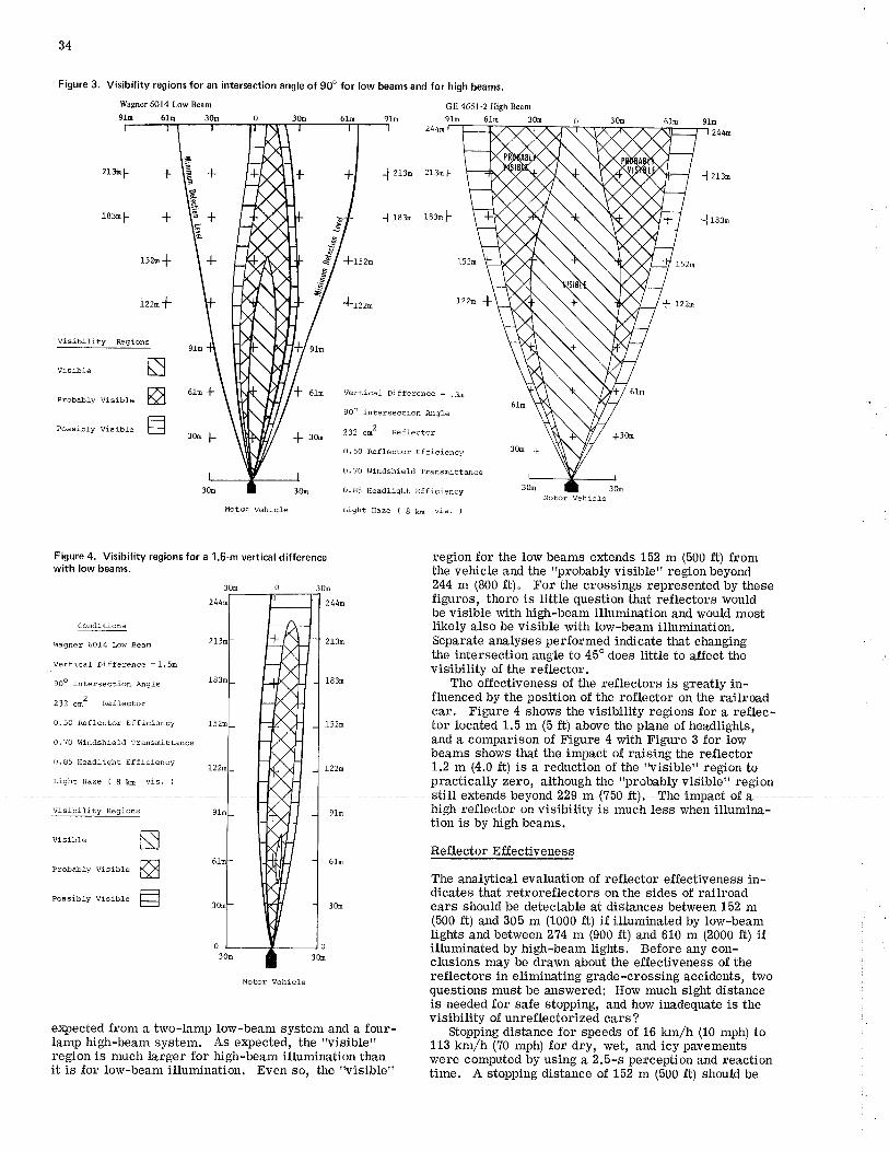
34
Figure 3. Visibility regions for an intersection angle of 90o for low beams and for high beams.
Wagner 6014 I¡w Bsn91¡ 6h 30r
GE 4651-2 High Beam
91d 618 3OE
213ú F J 213û 2130 l-
J 183m ls3mf
*rszt
4':',z^ 122a {
Vertical Diffe¡ence = .30
9Oo Intersection Angle
232 cm2 Reflector
0.50 Reflecto¡ Efficiency
0.?0 windshield transmittdce
0.85 Headl.ight Efficiency
Light Haze ( 8 kn vis. )
J zr:o
vi6íble
Probably VisibJ,e
Possj.bly visible
sntr
Motor Vehlcle
F igure 4. Visibility regions for a 1 .5-m vert¡cal d ifferencewith low beams.
* er'
+ 30^30o +
Ìlotor Vehi.cle
Con¿litions
Wagner 6014 bw Bean
Vertical Difference = L.5û
9oo lnèe¡section Àngle
232 c¡2 ReflectoÌ
0.50 Reflector Efficiency
0.70 windshield T¡asnittance
0.85 Headlight Efficiency
Light Hazê 1 6 ¡q vis. )
visibilj.¿y Regions
Visible
Probably visibLe
PossÍb1y vlsible
Moto¡ Vehicle
e).pected from a two-lamp low-beam system and a four-lamp high-beam system. As expected, the "visible"region is much larger for high-beam illumination thanit is for low-beam illumination. Even so, the "visible"
ñõ
=
region for the low beams extends 152 m (500 ft) fromthe vehicle and the "probably visible" region beyond244 m (800 ft)" For the crossings represented by thesefigures, there is little question that reflectors wouldbe visible wÍth high-beam illumination and would mostlikely also be visible with tow-beam illumination.Separate ar¡alyses performed indicate tbat changingthe intersection angle to 45o does little to a-ffect thevisibility of the reflector.
The effectiveness of the reflectors is greatly in-fluenced by the position of the reflector on the railroadcar. Figure 4 shows the visibility regions for a reflec-tor located 1.5 m (5 ft) above the plane of headtights,and a comparison of Figure 4 with Figure 3 for lowbeams shows that the impact of raising the reflector1.2 m (4.0 ft) is a reduction of the "visible" region topractically zero, although the "probably visible" region
high reflector on visibility is much less when illumira-tion is by high beams.
Reflector Effectiveness
The analytical evaluation of reflector effectiveness in-dicates that retroreflectors on the sides of railroadcars should be detectable at distances between 152 m(500 ft) and 305 m (1000 ft) if illuminated by low-beamlights and between 274 m (900 ft) and 610 m (2000 fi) ifilluminated by high-beam lights. Before any con-clusions may be drawn about the effectiveness of thereflectors in elíminåting grade-crossing accidents, twoquestions must be ¿mswered: How much sight distanceis needed for safe stopping, and ho"v inadequate is thevisibility of unreflectorized cars?
Stopping distance for speeds of 16 km/h (10 mph) to113 km/h (?0 mph) for dry, wet, and icy pavementswere computed by using a 2.5-s perception and reactiontime. A stopping distance of 162 m (500 ft) should be
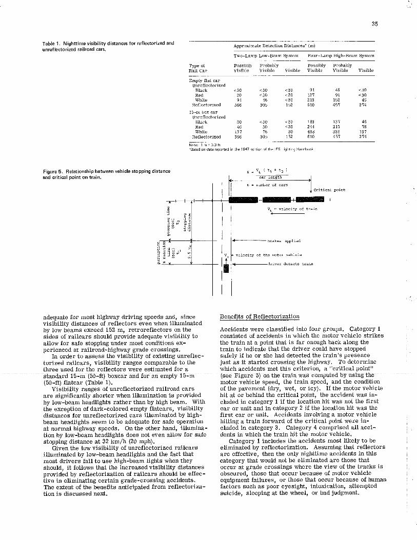
35
Table 1. N¡ghtt¡me visibility distances for reflectorized and
unref lectorized railroad cars.Approximate Detection Distances' (m)
Two-Lamp Low-Beam System Four-Lamp High-Beam System
Type ofRåiI Car
Possibly ProbablyVisible Visible Visible
Possibly ProbablyVisible Visible Visible
EmpW flat carUnrellectorized
BlackRedWhite
Rellectorized
15-m box carUnreflectorized
BlackRedWhite
Refl.ectorized
<30 <3030 <3091 46
366 305
30 <3046 30
13? ',16
366 305
<30<30<30152
<30<30
30152
9113?273610
183244488610
13?21333545',t
4691
\52451
<30<30
46274
4616
13?214
Note: 1 m=3.3ft." Based on data repoded in the 1 947 edition of the I ES L¡ghting Handbook.
Figure 5. Relationship between vehicle stopping distanceand critical po¡nt on train.
adequate for most highway driving speeds and, sincevisibility distances of reflectors even when illuminatedby low beams exceed 152 m, retroreflectors on thesides of railcars shor¡Id provide adequate visibility to
torized railcars, visibility ranges comparable to thethree used for the reflectors were estÍmated for a
illuminated by low-beam headlights and the fact thatmost drivers fail to use high-beam lights when they
Benefits of Reflectorization
Accidents were classified into four groups. Category 1
consisted of accidents in which the motor vehicle strikes
just as it started crossing the highway. To determinewhich accidents met this criterion, a "critical point"
are effective, then the only nighttime accidents in thiscategory that would not be eliminated are those that
allow for safe stopping under most conditions ex- the train at a point that is far enough back along theperienced at railroad-highway grade crossings, train to indicate that the driver could have stopped
In order to assess the visibility of existing unreflec- sa-fely if he or she had detected the train's presence
bTusingtll-(50-ft) flatcar (Table 1). motor vehicle speed, the train.speedr. and the condition
Visibilityrangesof unreflectorizedrailroadcars of thepavement(dry, wet, oricy). If themotorvehicleare significantly shorter when illumir¡,ation is provided hit at or behind the critical point, the accident was in-by low-beam headlights rather than by high beam. With cluded in category 1 if the location hit was not the firstthe exception of dark-colored empty flatcars, visibilíty car or unit and in category 2 if the location hit was thedistances for unreflectorized cars Ílluminated by high- first car or unit. Accidents involving a motor vehiclebeam headlights seem to be adequate for sa-fe operation hitting a train forward of ùhe critical point were Ín-at normal highway speeds. On the other hand, illumina- cluded in category 3. Category 4 comprised all acci-tion by low-beam headlights does not even allow for sa-te dents in which the train hit the motor vehicle.stopping distance at 32 km/h (20 mph). Category 1 includes the accidents most likely to be
Civen tire low visibility of unreflectorized railcars eliminated by reflectorization. Assuming that reflectors
should, it follows tÌ¡at the increased visibility distances occur at grade crossings where the view of the tracks isprovided by reftectorization of railcars should be effec- obscured, those that occur because of motor vehiclelive in elíminating certain grade-crossing accidents. equipment failures, or those that occur because of humanThe extent of the þenefits anticipated from reflectoriza- factors such as poor eyesight, intoxication, attempted
critical point
a-- brakes applied
velocity of the motor vehicle
tion is discussed next. suicide, sleeping at the $/heel, or bad judgment.
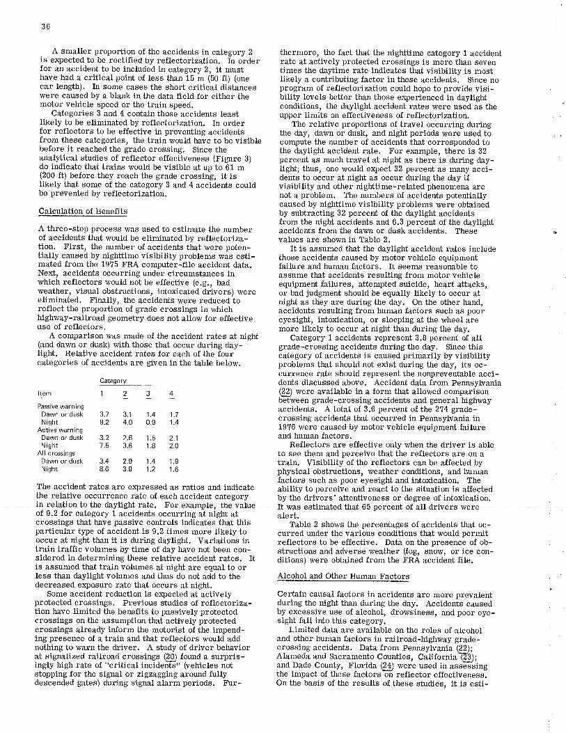
36
A smaller proportion of the accidents in category 2 thermore, the fact that the nighttime category 1 aecidentis enpected to be rectified by reflectorization. In order rate at actively protected croÀsings is more than sevenfor an accident to be included in category 2, it must times the daytinìe rate indicates that visibiuty is mosthave had a crÍtical point of less than 15 m (50 ft) (one likely a contributing factor in these accidents. Since nocar lengtù). In some cases the short critical distances program of reflectorization could hope to provide visi-were caused by a blank in the data field for either the bility levels better than those experÍènceùin daylightmotor vehicle speed or the train speed. conditions, ihe daylight accidenCrates were used as tåe
Categories 3 and 4 contain those accidents least upper límiis on effeciiveness of reflectorization.Iikely to be eliminated by reflectorization. In order The relative proportions of travel occurring duringfor reflectors to be effective in preventing accidents the day, dawn or dusk, and night periods were used tofrom these categories, the train would have to be visible computê the number oi accidents lhat corresponded tobefore it reached the grade crossing. Since the the daylight accident rate. For example, there is 82analytical studies of reflector effectiveness (Figure 3) percent is much travel at night as ttrere is during day-do indicate that trains would be visible at up to 61 m iight; thus, one would expeci32 percent as many acci-1?00 ft) before they reach the grade crossing, it is ¿entÁ to oécur at night as occur ãuring ihe day iilikely that some of the category 3 and 4 accidents could visibility and other-nighttime-related-phenomena arebe prevented by reflectoriz,ation. not a problem. The numbers of accidãnts potentially
calcuration of Benef*s ;i"Jf$lJ"l,"Tåi"î:J;:*'ift'JH;Ëi,i::ì¡btainedfrom the night accidents and 6.3 percent of the daylight
A three-step process was used to estimate the number accidents fiom üre dawn or duskãccidents. These -
of accidents that would be eliminated by reflectoriza- values are shown in Table 2.11o". First, the number of accidents tl¡at were poten- It is assumed Ûrat the daylight accident rates includetially caused by ryglq49 visibility problems was esti- those accidents caused by motõr vehicle equipmentmated from the 1975 FRA computer-file accident data. failure and huma¡ factors. It seems reasõnable toNext, accidents occurring under circumstances in assume that accidents resulting from motor vehiclewhich reflectors would not be effective (e.g., bad equipment failures, attemptediuicide, heart attacks,weather, visua-l obstructions, intoxicated drivers) were oi ¡àA judgment should be equally likeiy io occur ateliminated. Finally, the accidents were reduced to night as thãy are during the day.
- On the other hand,
reflect the proportion of grade crossings in which ac-cidents résulting from human factors such as pooíhighway-railroad geometry does not allow for effective eyesight, intoxicatìon, or sleeping at the wheel àreuse of reflectors. more likely to occur át night than during the day.
A comparison was made of the accident rates at night Category 1 accidents represent B.g pãrcent of alt(and dawn or dusk) with those that occur during day- grade-ciossing accidents during the day. Since thislight. ReÞtive accident rates for each of the four ðategory of acõidents is caused primarily by visibilitycategories of accidents are given in the table below, problems that should not exist düring the day, its oc--
cumence rate should represent the nonpreventable acci-categorv dents discussed above. Accident data from PennsylvaniaItem L ? q L .Ç) were available in a form that allowed comparison
Pass ve warn ngDawn or dusk 3.7 3.1 1 .4 1 .7Night g.2 4.0 0.9 1.4 crossing accidents that occurred in Pennsylvania in
Active warning 1976 were caused by motor vehicle equipment failureDawn or dusk 3.2 2.6 1.5 2.1 and human factors.Night 7.5 3.6 f .B 2.o Reflectors are effective only when the driver is able
All crossings to see tllem and perceive that the reflectors are on aDawn or dusk 3.4 2.9 1.4 1.9 train. Visibilíty of Ûre reflectors can be affected byNight 8'6 3'9 1.2 1.6 physical obstruétions, weather conditions, a¡rd human
rhe accidenr rares are expressed as rarios and indicate liTlirir":rli3:ti:äåHj3ilfrflJ:tr?f"iiji"* Jå:,"dthe relative occurrence rate of each accident category by thé drivers'attentiveness or degree of intoxication.in relationlolhe rlay-lighlrate- Jor example, lhe value l¿ ças estirnated tùat 65 percent oiãlLdrivers¡,vereof 9.2 for category 1 accidents occurring at night at alert.crossings that have passive controls indicates that this Table 2 shows the percentages of accidents 6at oc-particular type of accident is 9.2 times more likely to curred under the variõus conditions that would permitoccur at night than it is during daylight. Variations in reflectors to be effective. Data on the presencè of ob-train tra"fiic volumes by time of day have not been con- structions and adverse weather (fog, snow, or ice con-sidered in determining these relative accident rates. It ditions) were obtained from ttre ÈnÁ accidãnt file.is assumed that train volumes at night are equal to orless than daylight volumes and thus do not add to ttre Alcohol and Other Human Factorsdecreased exposure rate that occurs at night.
Some accident reduction is e4pected atãctively Certain causal factors in accidents are more prevalent I
protected crossings. Previous studies of reflectoriza- during the night than during the day. Accidents causedtion have limited the benefits to passively protected by excessive use of alcohol, drowsiness, alrd poor eye- l
crossings on the assumption that actively protected sight fall into this category. l
crossings already inform the motorist of the impend- Limited data are available on the roles of alcohol ,
ing presence of a. train and that reflectors woutd add and other human factors in railroad-highway grade- ]
nothing to warn the driver. A study of driver behavior crossing accidents. Data from Pennsylvania (22); ;
at signalized railroad crogsingq Q!) found a surpris- Alameda and Sacramento Counties, California@);ingly high rate of "critical incidents" (vehicles not and Dade County, Florida (ZÐ were used in ass-ssingstopping for the signal or zígzagg¡ng around fully the impact of these factorsõã reflector effectiveness.descended gates) during signal alarm periods. Fbr- On the basis of the results of these studies, it is esùi-
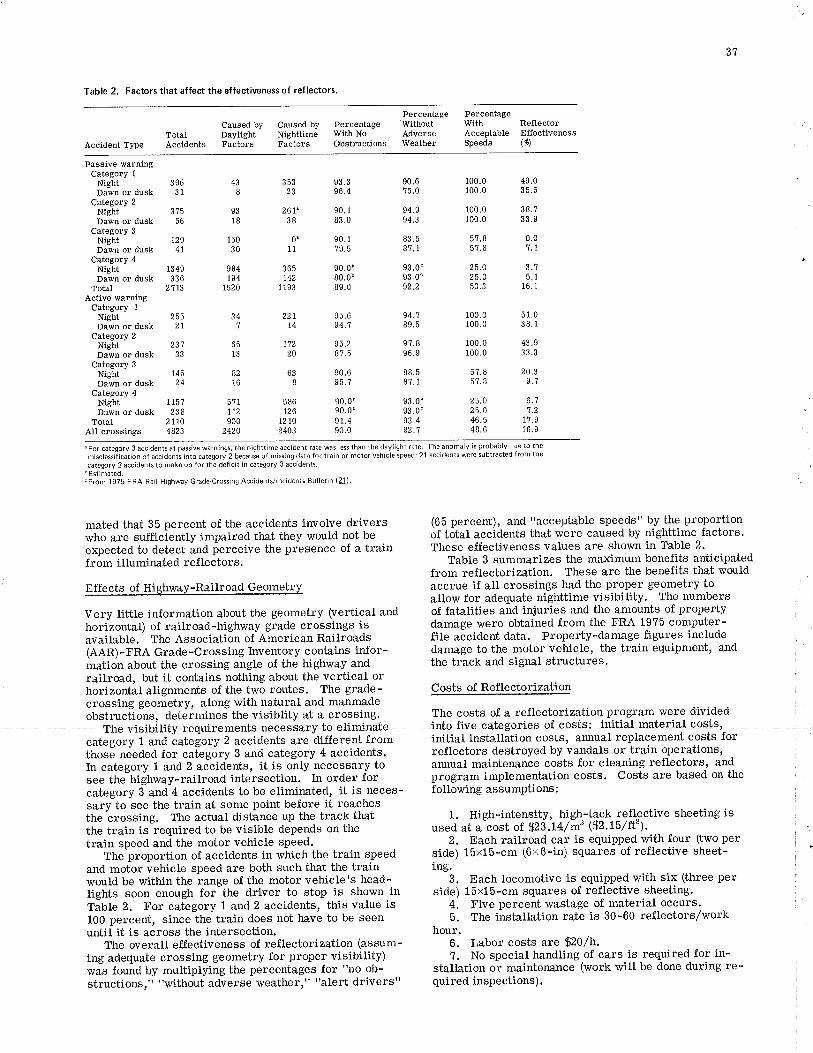
37
Table 2. Factors that affect the effectiveness of reflectors.
TotalAccidentType Accidents
Caused by Percent¿geNighttime With NoFactors Obstructions
With RellectorAcceptablê EflectivenessSpeeds (#l
Caused byDaylightFactors
WithoutAdverseWeather
Passive warningCategory I
NiehtDawn or dusk
Category 2NiehtDawn or dusk
Category 3NightDawn or dusk
Category 4NightDawn or dusk
TotalA.ctive wârning
Category 1
NtghtDawn or dusk
Category 2NightDawn or dusk
Category 3
NightDawn or dusk
Category 4NiehtDawn or dusk
TotalAll crossings
39631
3?556
1294L
1349336
z',t13
2552l
23133
14524
1 15?238
27t04823
5?1tL2900
2420
63I
586t26
12 102403
90.6?5.0
94.994.3
83.58'.1.7
93.0"93.0"s2.2
94.789.5
9?.896.9
88.587.1
93,0"93.0"93.4
93.396.4
90.183.0
90.179.5
35323
267"38
0"11
365742
1193
22tt4
17220
43I
9318
15030
984194
1520
34,|
6513
8216
100.0 49.0100.0 35.5
90.0b80.0b89.0
95.694.'.|
95,287.5
90.695. ?
100.0 38.?100.0 33.9
5?.8 0.05?.8 '.t.t
25.0 3.?25.0 5.150.3 16.1
100.0 51.0100.0 38.1
100.0 43.9100.0 33.3
20.39.7
6.?'t.2
1?.916.9
90.0ù90.0b91.490.0
5?.8
2 5.025.046.548.6
" For categorv 3 accidents at passive warn¡ng€, the n¡ghttime accident rate was less than the daylight râte. The anomaly is probably Je to the
mi$lassificat¡on of accidents into categort2 becauJe of missing data for train or motor vehicle speed; 21 accidents were subtrâcted from the
category 2 acc¡dents to make up for the def¡cit in category 3 accidents.b Estimâted." From 1 975 F RA Rail-H¡ghway Grade-Crossing Accident$/lnciden$ Bulletìn {2f)
mated that 35 percent of the accidents involve driverswho are sufTiciently impaired that they would not bee)rpected to detect and perceive the presence of a trainf rom illuminated reflectors.
Effects of Highway-Railroad Geometry
Very little information about the geometry (vertical andhorizontal) of railroad-highway grade crossings isavailable. The Association of American Railroads(AAR) - FRA Grade -Crossing tnventory c ontains inf or-mation about the crossing angle of the highway andrailroad, but it contains nothing about the vertical orhorizontal alignments of the two routes. The grade-crossing geometry, along with natural and manmadeobstructions, determines the visiblity at a crossing.
(65 percent), and "acceptable speeds" by the proportionof tõtaf accidents that were caused by nighttime factors.These effectíveness values are shown in Table 2.
Table 3 summarizes the maximum benefits anticipatedfrom reflectorization. These are the benefits that wouldaccrue if all crossings had the proper geometry toallow for adequate nighttime visibility. The numbersof fatalities and iniuríes and the amounts of propertydamage were obtained from the FRA 1975 computer-file accident data. Property-damage figures includedamage to the motor vehicle, the train equipment, andthe track and signal structures.
Costs of Reflectorization
The costs of a reflectorization program were divided
initial installation costs, arutual replacement costs forreflectors destroyed by vandals or train operations,armual maintenance costs for cleaning reflectors, andprogram implementatíon costs. Costs are based on the
1. High-intensity, high-tack reflgctive sheeting isused at a cost of fi23.14/nf ($2.15lft).
2, Each railroad car is equipped r¡¡Ìth four (two perside) 15x15-cm (6x6-in) squares of reflective sheet-ing.
3. Each locomotive is equipped with six (three perside) 15x15-cm squares of reflective sheeting.
4, Five percent wastage of material occurs.5. The insbffation rate is 30-60 reflectors/work
hour.6. Labor costs are $20/h.7. No special handling of cars is required for in-
stallation or maintenance (work will be done during re-quired inspections).
category 1 and category 2 accidents are different fromthose needed for category 3 and category 4 accidents.In category t and 2 accidents, it is only necessary tosee the highway-railroad intersection. In order forcategory fand-4 accidents to be eliminated, it is neces- following assumptions:sary to see the train at some point before it reachesthe crossing. The actual distance up the track thatthe traín is required to be visible depends on thetrain speed and the motor vehicle speed.
The proportion of accidents in which the train speedand motor vehicle speed are both such that the trainwould be within the range of the motor vehicle's head-lights soon enough for the driver to stop is shown inTable 2. For category 1 a¡d 2 accidents, this value is100 percent, since the train does not have to be seenuntil it is across the intersectíon.
The overall effectiveness of reflectorization (assum-ing adequate crossing geometry for proper visibility)was found by multiplying the percentages for "no ob-structionsr" "without adverse weatherr" "alert drivers"
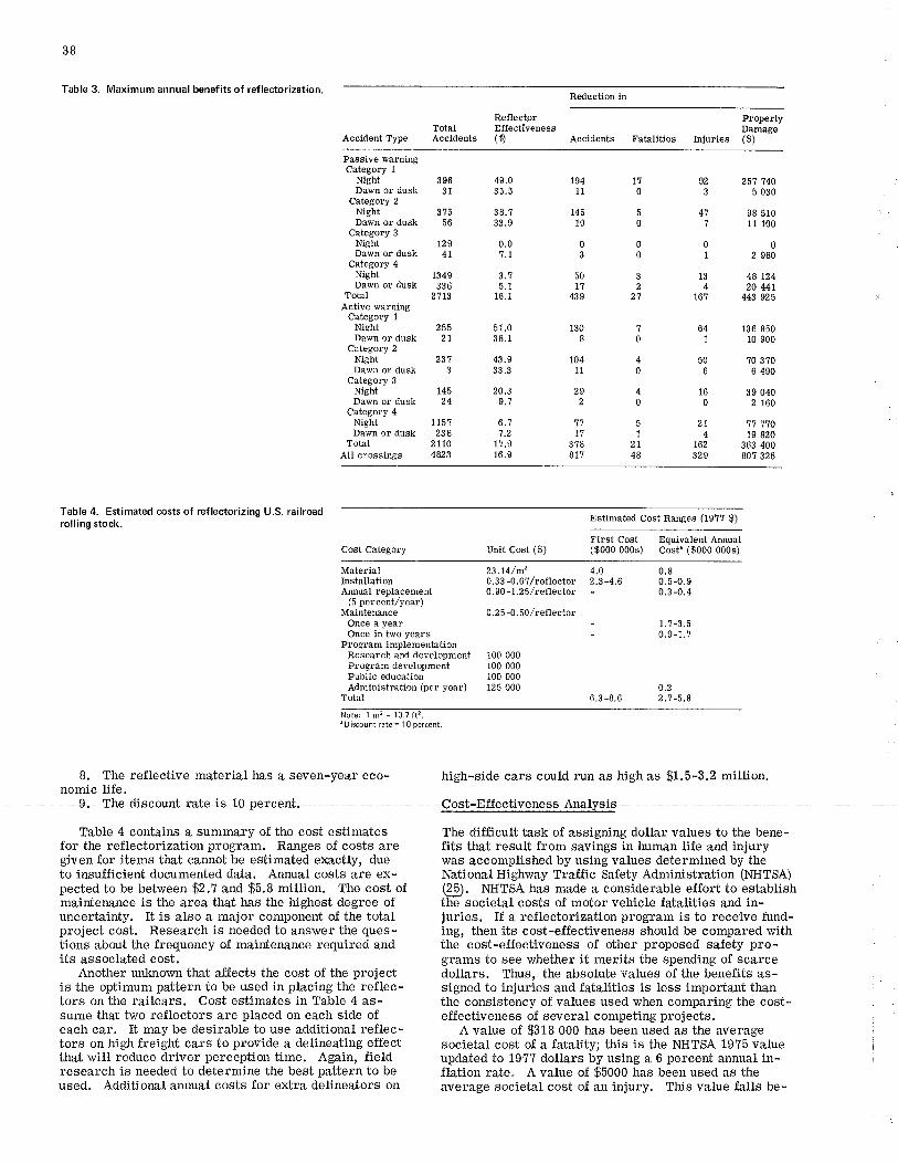
3B
Table 3. Maximum annual benefits of reflectorizat¡on.
Reflector Property
Reduction in
Accident Type Accldents ($) Accidents Fatalities Injuries ($)
Paasive warningCâtegory I
NiehtDâwn or dusk
Cãtegory 2NightDawn or dusk
Category 3NightDawn or dusk
Category 4NightDawn or dusk
TotaIActive warning
Category 1
NightDawn or dusk
Câtegory 2NightDawn or dusk
Category 3NightDawn or dusk
Category 4NightDawn or dusk
TotåIAII crossings
923
471
01
13
416?
194 t711 0
145 51900030
503772
439 21
396 49.03 1 35.5
3?5 38.756 33.9
129 0.047 1.7
641
506
160
2t4
t62329
251 7405 030
98 51011 100
1349336
2713
25527
2313
74624
1157238
21104823
3.15.1
16.1
5 1.038.1
43.933.3
20.39.7
o. t7.2
1?.916.9
130 780
104 411 0
29420
11 57',t 1
3?8 2t81? 48
02 980
48 12420 447
443 525
136 85010 900
?0 3?06 490
39 0402 160
11 11019 820
363 400807 325
Table 4. Est¡mated costs of ref lectorizing U.S. railroadrolling stock. Estimated Cost Ranges (197? $)
First Cost Equivalent Amual($000 000s) Cost' ($000 000s)Cost Category Unit Cost ($)
MateriâlInstallationAmual replacement
(5 percent/year)Maintemnce
Once a yearOnce in two years
Program implementationResearch and developmentProgram developmentPublic educationAdministration (per year)
Totâl
23.74/m20.33 -0,6?/reflector0.90 -1.25/rellector
0.2 5 -0.50/reflector
100 000100 000100 000125 000
4.0 0.82.3-4.6 0.5-0.9- 0.3-0.4
- 1.?-3.5- 0.9-1.7
0.26.3-8.6 2.1-5.8
j'Jlå;,1"ï,'"; 1oi'o Il;"" ",.
8. The reflective material has a seven-year eco- high-side cars could n¡n as high as $1.5-3.2 míllion.nomic Ufe.
I- The4iseount r¿te is 10 pe+eent#ost-Effeetiveness Arra1ysi
Table 4 contains a summary of the cost estimatesfor the reflectorization program. Ranges of costs aregiven for items that cannot be estimated exactly, dueto insufäcient documented data. Annual costs are ex-pected to be between $2.7 and $5.8 million. The cost ofmaintenance is the area that has the highest degree ofuncertainty. It is also a ma¡or component of the totalproject cost. Research is needed to answer the ques-tions about the frequency of maintenance required andits associated cost.
Another unknown that a-ffects the cost of the projectis the optimum pattern to be used in placing the reflec-tors on the railcars. Cost estimates in Table 4 as-sume that two reflectors are placed on each side ofeach car. It may be desirable to use additional reflec-tors on high freight cars to provide a delineating effectthat will reduce driver perception time. Again, fieldresearch is needed to determine the best pattern to beused. Additional annual costs for extra delineators on
The difficult task of assigning dollar values to the bene-fits that result from savings in human life and injurywas accomplished by using values determined by theNational Highway Tra-tfic Sa-tety Administration (NHTSA)(3Ð. NHTSA has made a sonsiderable effort to establishthe societal costs of motor vehicle fatalities and in-juries. If a reflectorization program is to receive fund-ing, then its cost-effectiveness should be compared withthe cost-effectiveness of other proposed safety pro-grams to see whether it merits the spending of scarcedollars. Thus, the absolute values of the benefits as-signed to injuries and fatalities is less important thanthe consistency of values used when comparing the cost-effectÍveness of several competing projects.
A value of $318 000 has been used as the averagesocietal cost of a fatality; this is the NHTSA 1975 valueupdated to 1977 dollars by using a 6 percent arurual in-flation rate" A value of $5000 has been used as theaverage societal cost of an injury. This value falls be-
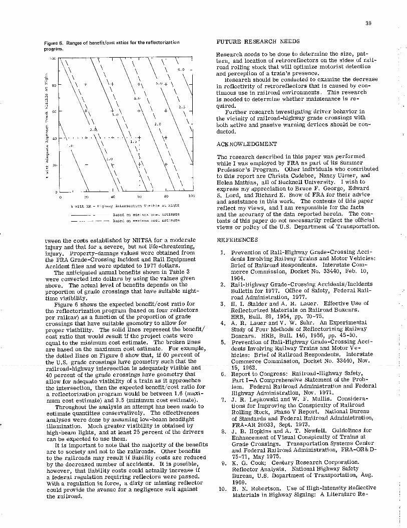
Á.i
x60odtsH
IooþÊ¿o
aoE¿20!3
Figure 6. Ranges of benefit/cost rât¡os for the reflector¡zat¡onprogram,
ro0
=go
o20406080
t with RR - Highway Inëersection Visible at Night
\ \', \ \' \ \\ \\, \'\ \ \ 6.0\ \\, \'\ \ r\ + \\¡ \ìr u'l*\\ \\, \ '1 \ \
\, \')', '\",
\'.\ \\, \)." \ \, \\ \2.o\ \', \ \' .+'\\. .*.\.\. .* \+r' \ \ir \"
.- \ \,, \",\ :\', \ \
39
FUTURE RESEANCH NEEDS
Research needs to be done to determine the size, pat-tern, and location of retroreflectors on the sides of rail-road rolling stock that will optimize motorist detectionand perception of a train's presence.
Research should be conducted to examine tùe decreasein reflectivity of retroreflectors that is caused by con-tinuous use in railroad environments" This researchis needed to determine whether maintenance is re-quired.
Further research investigating driver behavior inthe vicinity of railroad-highway grade crossings witltboth active and passive warning devices should be con-ducted.
ACKNO\ryLEDGMEI{f
The research described in this paper was performedwhile I was employed by FRA as part of its SummerProfessor's Program. Gher individuals who contributedto tåis report are Christa Cudebec, Nancy Ulmer, andHelen Mathias, all of Bucknell University' I rvish toexpress my appreciation to Bruce F. George, EdwardS. Lord, and Richard E. Srow of FRA for their adviceand assistance in this work. The contents of this paperreflect my views, and I am responsible for the factsand the accuracy of the data reported herein. The con-tents of this paper do not necessarily reflect the officialviews or policy of the U.S. Department of Transportaùion.
REFERENCES
1. Prevention of Rail-Highway Grade-Crossing Acci-dents Involving Railway Trains and Motor Vehicles:Brief of Railroad Respondents. Interstate Com-merce Commission, Docket No. 33440, Feb. 10,
1964.2. Rail-Highway Grade -Crossing Accidents,/Incidents
Bulletin for 1977. Office of Safety, Federal Rail-road Administration, 19?7.
3. H. I. Stalder and A. R. Lauer. Effective Use ofReflectorized Materials on Railroad Boxcars.HRB, Bult. 89, 1954, PP' ?0-75.
4. A. R. Lauer andV. 1{. Suhr. An Ex¡lerimentalStudy of Four Methods of Reflectorizing RailwayBoxcars. HRB, Bull. 146, 1956, pp' 45-50.
5. Prevention of Rail-Highway Grade-Crossing Acci-dents Involving Railway Trains and Motor Ve-hicles: Brief of Railroad Respondents. Interstate
6. Report to Congress: Railroad-Highway Sa-fety,
Part I-A Comprehensive Statement of the Prob-lem. Federal Railroad Administration and FederalHighway Administration, Nw. 1971.
?. J. R. Lepkowski and W. F. Mullis. Considera-tions for Improving the Conspicuity of RailroadRolling Stock, Phase V Report. National Bureauof Standards and Federal Railroad Administration,FRA-AR 20033, SePt. 19?3.
8. J. B. Hopkins a¡rd A. T. Newfell. Guidelines forEnhancement of Visual Conspicuity of Trains atGrade Crossings. Transportation Systems Centerand Federal Railroad Administration, FRA-OR&D-15-7t, May 197õ.
9. K. G. Cook; Century Research Corporation.Reflector Analysis. National Highway Sa-fety
Bureau, U.S" Department of Transportation, Aug.1969.
10. R. N. Robertson. Use of High-Intensity ReflectiveMaterials in Highway Signing: A Literature Re-
the U.S. grade crossings have geometry such that the Commerce Commission, Docket No' 33440, Nov. I
railroad
_::::: :l i::iTi :::: :::ü::
tween the costs established by NHTSA for a moderateinjury and that for a severe, but not life-threatening,injury. Property-damage values were obtained fromthe trR'A Grade-Crossing Incident and Rail EquipmentAccident files and were updated to 197? dollars.
The anticipated annual benefits shown in Table 3
were corrverted into dollars by using the values givenabove. The actual levet of benefits depends on theproportion of grade crossings that have suitable night-time visibility.
Figure 6 shows the e:çected benefit,/cost ratio forthe reflectorization program (based on four reflectorsper railcar) as a function of the proportion of gradeõrossings that have suitable geometry to allow forproper lisiuiuty. The solid lines represent the benefit/cost ratio that would result if the project costs wereequal to the minímum cost estimate. The broken linesare based on the ma:rimum cost estimate. For example,the dotted lines on Figure 6 show that, if 60 percent of
40 percent of the grade crossings have geometry tlratallõw for adequate visibility of a train as it approachesthe intersection, then the e4pected benefit'/cost ratio fora reflectorization program would be between 1.6 (maxi-mum cost estimate) and 3.5 (minimum cost estimate)'
Throughout the analysis an attempt has been made toestimate quantities conseruatively. The effectivenessanalyses were done by assuming low-beam headlightillumination. Much greater visibility is obtained byhigh-beam lights, and at least 25 percent of the driverscan be ex¡lected to use them.
It is important to note that the majority of the benefitsare to society and not to the railroads. Other benefitsto the railroads may result if liability costs are reducedby the decreased number of accidents. It is possible,however, that liabitity costs could actually increase ifa federal regulation requíring reflectors were passed.With a regulation in force, a dirty or missing reflectorcould provide the avenue for a negligence suit againstthe railroad.
40
11.
12.
13.
L4.
15.
16.
t7.
20.
2L.
22.
23.
18.
19.
view. Virginia Research Couneil, Charlottesville,Aug. 19?8.C. T. Hare and R. H. Hemion. Head-Lamp-BeamUsage on U.S. Highways" Southwest Rcscarch In-stitute, San Antonio, TX, and Federal HighwayAdministration, Rept. No. AR-666, Dec. 1968.N. T. Cox. The Effect of Dirt on Vehicle Head-Lamp Perform¿ùnce" U, K. Transport and RoadResearch Laboratory, Crowthorne, Berkshire,England, Rept. LR 240, 1968.K. Rumar. Dirty Headlights: Frequency andVisibility Effects. University of Uppsala, Uppsala,Sweden, Rept. 136, 1973.H. L. Woltman and W. P. Youngblood. IndirectFactors Affecting Reflective Sign Brightness. TRB,Transportation Research Record 611, 1977, pp.35-37.P. L. Connolly. Vision, Man, Vehicle, and High-way. In The Prevention of Highway Injury, High-way Safety Research hstitute, Ann Arbor, MI,1967, pp. t22-t49.W. Heath and D. M. Finch. Effect of Tinted Wind-shields and Vehicle Headlighting on Night Visibility.HRB, Bull. 68, 1953, pp. 1-15.E. Wolf, R. A. McFarland, and M. ZigLer. In-fluence of Tinted Windshield Glass on Five VisualFunctions. HRB, Bull. 255, 1960, pp. 30-46.IES Lighting Handbook, 5th ed. IlluminatingEngineering Society, New York, 19?2.F. C. Breckenridge and C. A. Douglas. Develop-ment of Approach and Contact-Light Systems.Illuminating Engineering, Vol. 40, 1945, p. 785.G. J. S, Wilde and others. An Observational Studyof Driver Behavior at Signalized Railroad Cross-ings. Ca:radian Institute of Guided Ground Trans-port, Kingston, Ontario, Feb. 19?6.Rail-Highway Grade -Crossing Ac cidents/IncidentsBulletin for 1975. Office of Sa-fety, Federal Rail-road Administration, 1975.Statistical Summary for the Period January throughDecember 1976, Encompassing All RailroadCrossing Accidents. Pennsylvania Department ofTransportation, Hamisburg, 1917.J. A. Waller. The RoIe of Alcohol in Fatal Col-lisions with Trains. Northwest Medicine, Sept.1968, pp. 852-856.Alcohol, Violence, and the Automobile. MedicalExaminer's Office, Dade County, FL, 1968.19?5 Societal Costs of Motor Vehicle Accidents.National Hi ghway Tra-ffic Safety Admini strati on,U.S. Department of Transportation, Dec. 1976.
could be concentrated at railroad terminals in areas ofhigh unemployment. This project would appear to in-volve direct federal funding because of the mobile r¡atureof the railroad vchiclcs, which are not restricted to onestate.
It appears, however, that a certain effect thatweakens the case for reflectorization was not con-sidered, In a substantial percentage of cases, head-lights from highway tra^tfic in the opposing directionca¡ be seen through the spaces betrveen the movingtrain cars, or under the bodies of the cars between thewheels, thus ereating a very eye-catching effect thatis more visible than the reflectors, and this is an addi-tional circumstance under whÍch the reflectors wouldnot be effective.
In category 3 and 4 accidents, the locomotive's head-light would normally be visible long before the reflec-tors, because its visibility does not depend on reflec-tivity and because it is much higher off the ground thanthe reflectors. The illumination of objects around thecrossing by the locomotive headlights as the train ap-proaches may also attract more attention to the traintha¡ the reflectors would, especially since this effectprecedes the arival of the train,
I am skeptical that reflectors on the cars couldcreatea significant increase in attracting a motorist's atten-tion when the crossing is protected by gates (whichnormally have flashing lights on the gate in addition tothose on the mast); I believe, therefore, that accidentsoccurring at gated crossings are very unlikely to beprevented by reflectors. In some cases, the gate mayactually block the view of the reflector. Is there anyreason that the distinction between gates and flashersa¡d flashers alone was not made? Perhaps the acci-dents that occur at gated crossings should be taken asthe limit of the effectiveness of reflectors, rather tha¡daylight conditions.
Perhaps a further analysis of category 2 accidentsshould be made. The paper indicates that in "somecases" accidents fell into this category because of a"blank in the data field." Notes in Tabte 2 indicatethat some adjustment was made, but no justificationis given. It would appear that a similar adjustmentwould be needed in the "active ',varning" category.
More than four reflectors per car (two per side)would proba.bly be needed on cars more than 18 m (60 ft)long. Common types of cars, such as piggyback, auto-mobile racks, and automobile parts cars are about 26-27 m (85-90 fi) long. It would seem that the maximumdistance between reflectors should be about I m (30 ft).I feel that answers to these questions, which reflect
24.
25.
botå positively and negativelyon tåegojeefare \vorth-evaluating.
DiscussionLouis T. Cerny, Erie Western Railway Company,Huntington, Indiana
The reflectorization of railroad rolling stock appears tome to be a good idea. Certain factors would make itappear even more favorable than the study shows. Inmost cases the reflectors would be moving, causingincreased probability of detection, and more than onereflector is likely to be in view at all times. I do notbelieve these additional favorable efÏects were takeninto consideration.
Another favorable aspect is that the cleaning andapplication of the reflectors is a low-skill job and, be-cause of the natio¡ral nature of the car fleet, the work
John B. Hopkins, Transportation Systems Center, U.S. De-partment of Transportation, Cambridge, Massachusetts
McGinnis has carried out a comprehensive and pene-trating analysis that appears to achieve as definitive anans\¡/er as can reasonably be expected concerning thecosts and benefits of railcar reflectorization. His paperbrings out many of the uncertainties that are inherentto our basic lack of knowledge concerning accidentcausation, driver behavior, reflector degradation inthe railrq.d environment, etc. I¡r most cases I find hisassumptions and estimates to be quite reasonable. Itis my purpose in these brief comments to address onlya few aspects in which I feel the ambiguities are so
4t
important as to warrant special attention. MI¡ aim is scenario, ultlt ful1 consideration of the limitations on
nodio ériticize, r.or I havô no substantive complaints potential safety effectiveness described above, reason-
with the study. Rather, I wish to emphasize s-ou"ces able minimum and maximum benefits might be approxi-of uncertainti trtat I coúslder to be relevurt to inter- mately 25 and ?5 perccnt of the values projected in the
pretation of the results, particutarly with reference to paper. The net effect of these modifications, wlich re-îo"*ol"tio' of policy in this area. ãuãe both costs and benefits, is relatively small; I
McGiruris has effectively placed an upper bound (the infer a subjective "most- l jkely" benefit-cost ratio -
¿avüáttt accident rate) on mË sa¡ety benifits that might probably in excess o.t f .o litt less than 2.0. It should
¡e"asîociated with reÍlectorization. The question thén be noted at this point that the benefits accrue primarilybecomes one of estimating appropriate reductions from to society ín general and only to a limÍted degree to
this value due to various limitations. One could quibble the raihôads. Installation at railroad expense would
over matters of headlight aim, the assumption of low- thus almost certainly have a benefit-cost ratio for them
¡uu* op"t"tion, stopping distances, etc. However, well below 1.0. From either the societal or railroad
these are minor points, änd they teir¿ to balance onâ viewpoint, t^h9re..m1y well be other investments in
another. More complex is the need to assess whether crosèing Safety that- can be. .expected to yie.ld greater
lnoiã accioents ideniified as relevant are truly caused benefits. To keep this matter in perspective, note
by visibility problems of a type that could Ue äitigateO !Þ! tl" above estimates imply a maximum saving of
ry reflectois, vry suljeciiväviewis that reflectõr ef- 12 to 36 lives/year, p.rior.to.correction for geometric
fectiveness as shown in Table 2 is somewhat optimistic, factors that could easily diTinish the benefits by another
or at least represents only a reasonable upper bound, factor of 2 to 4. The net effect on crossing sa'fety would
parii.ur""rv a:t crossings l¡at h"vu active-ïarning syr- thus be an improveme.nt 9T approximately 1-2 percent'
ié*". Foi example, Iïnd it quite untikely ttrat 11 per- Thus, while reflectorization may ultimately prove to be
cent of the drivers who fail to iespond to conventioùI a worthwhile step, with significant benefits, it_ does
railroad-crossing flashing lights (some with gates) for not appear to be of major importance to crossing sa-fety
night-related reaÈons will be deterred any more effec- in general'tiv"erv ¡v railcar reflectors. This is a re-tativety im- Í am in full agreement with the research needs
portänt question, since Table 3 shows tbat 46 percent McGinnis has identified, and I would only add reflectorãt tire expected áccident reduction is to occur ãt such type and cost to the reflector optimization study' At
erossings. tirè same time, the T^l?iiygly limited promise o.f reflec-A faðtor that a"ffects both cost and effectiveness is torization, and the difficulty of obtaining definitive
reflector maintenance. One can envision many possible answers to these questions, seems to warrant only a
maintenance scenarios, each with its own benefil-cosù modest priority for such research,
implications. To my mind, the most realistic assump-tion is that of no maintena¡rce at all' This substantiallyreduces estimated costs (by 33 percent for the "mini-mum cost" case and by 60 pereent for "maximum cost"),while having a negative but indeterminate effect on
safety. (It is appropriate to mention here that othertypes of reflectors could be used. For example, plasticdevices used as highway delineators have somewhat less
Otto F. Sonefeld, Atchison, Topeka, and Santa FeRailway CompanY, Chicago, Illinois
äãåiilorä Jt,å:riï:ru}]iliilii"J * tüiJ äõp*r'"át'"", u"t As lvlcGinnis indicated, the rerlectorization or railroad^i ^ ^¿ ^4 l^L^+^ *^-" #i rúaarolling stock has been the subject of debate many times
over the past few decades. Arguments favoring re-flectorizátion have generally failed to show significantevidence of the effectiveness of this approach, par-ticularly when compared with substa¡rtial argument infavor of other grade-crossing safety activities.
The McGinnis study is perhaps the most compre-
active-wárninþ systems and to achieve mõre widespread hensive look at this subject to date, although it leaves
installation of train-activated devices. Reflectorizedcrossbucks, improved flashing lights, and increased
they appear to perform well in a rather dirty environ-*ent for many years without cleaning or replacement.)
In the context of policy formulation, another set offactors takes on real significance. These involve theeffects of other activities that are expected to improvegrade-crossing sa"tety. For example, there are nowunder way major efforts to improve both passive- and
many questions unansrvered. The problem, in myopinion, is in the attempt to draw fairly firm conclu-
Serious government and industry consideration is cur-rently belng given to widespread installatio¡ oflocomotivelmounted strobe lights, which should do
all that can be done through vísibitity enhancement to e><plored'
prevent the accidents Mcõinnis placðs in categories 3 - ._,The part of the study that deals with reflector visi-
and 4 (collisions occurriná ctosô to the front of the bility distances appears to be well documented and rea-
train). These repre."nt g"t percent of the total esti- sonable. one of the shortcomings of previous proposals
*"tu¿ t"t"uty reãuction, whieh would thus be eliminated for reflectorization has been the inability of engineering-
,.-, pot""tiri reflector úenefit. There could also be ¿ grade reflective material to function effectively in the
uãñtigniri"ant impact ãn categorles 1 and 2. (It is severe railroad environment without diligent mainte-
not claimed that strobé rigrtt" .,räu necessarily pievent nance.- The introduction of high-intensity reflective
these accidents. Howevãi, ior potentiat colúsions material would seem to diminish this problem, although
n"r" tt" locomotive, if str'obes ão not help, reflectors it is not clear that even the use of that material would
are unlikely to succeed either.) produce the 0.50 rate of efficiency used in the study.
The basic conclusions of thé paper, as presented in The recommended location for the reflective material
Figure 6, assume maximum and miniinurncost esti- is the most severe erwironment on a railcar.*Ët"r. i suggest that for a more realistic estimate This is not to say that diligent maintenance could not
one should uãã a single no-maintenance cost assumption overcome this problem; how9v91, ex¡lerience in the .
thesubþct. sionr- frorn data t*at ds nst lend themselvesJs sueh de- l
tailed analysis. McGinnis has done a commendable job I
under these circumstances, but it has required makingcertain assumptions that I feel should be more critically
that still has two curves, based on minimum and maxi-mum estimates of benefits. For the no-maintenance
automatic car identification (ACI) program does not in-dicate the capability or will of the rail industry to
42
properly n¡aintain the reflective material unless thereis a return to the industry far greater than that providedby the ACI program, St¡ch benefits are not apparent.In any event, the long-term efTectiveness of tt¡i materialseems open to question. Certainly, the cost-benefitratios would be a-tfected by increased maintena¡ce re-quirements.
In the same vein, although the report acknowledgesthat a motorist may have a problem perceiving therecommended light source as a railroad train on acrossing, the perception time used in the report appearsto assume that a motorist immediately recognizes the
requires more rigorous enamination.McGinnis correctly suggests further research into
various aspeots of this matter. I agree wittr these sug-gestions and, as indicated by my comments in this dis-cussion, I would also suggest further refinements orclarifÍcations of some of the critical factors involvedin the development of costs and benefits associated rvitlrthis subject.
light source as a crossing hazard a¡d comes to a prompthali. I would suggest that a train crossing is unusual Atf thOf rS ClOSa11. eenough in the total tra-fTic scheme ttr,at a longer percep-tion time would be required to recognize it for what it is. It does not seem t}at blinking lights from opposÍng- In developing the "ctitical point" used as the basis headlights shining tlrough ttrã spaces betwee¡ movingfor analysis of the FRA accident reports, apparently railcars will a-t¡eõt the iesults ôt tiris study; if whatvehicle speeds as stated on the reports are used. If so, Cerny says is true, and I think it is, then älivers aidedit appears tåat vehicle speeds would tend to be con- by thóse åtir*ing lights are alreadyieeing the train andsistently understatedr. inasmuch as the accident reports are sa-fely stoppingl Thus, they are not blecoming FRArequire speed at the time of impact, not üre approach accident itatiÀticJanA would nol be touched by thõspeed at which the decision to stop must be made. U I potential benefits of reflectorization.understand the rationale behind development of the Cerny indicated a concern about the impact of loco_c-ritical point, this would then have the efÏect of placing motive headlights on potential reductions ôf category 3that point further back in the train and thus of reducing and 4 accidenis from reflectorization, There aré piob-botlt the number of accidents shown in categories 1 and lems Ín the use of locomotive headlights as a means of2 and the number of vehicles ttr,at would realize any informing motorists about the impenãing danger of anbenefits from reflectorization. approaching train. Locomotive hìaOUgñts are placed
Highly important are the assumptions in tåis study ciõse togetñer, giving the impression õf a singÍe light,that result in a finding tfiat category 1 accidents at and are aimed'in a very narrow beam. First;the tací<active-warning crossings are 7.5 times more likely to of space between the two lamps does not allow aoccur at night than during daylight. This further motorist to judge distance inihe way he or she ca¡rtranslates to a finding that reflectorization would pre- with widely äpaãeA automobile Þmpä. Second, thevent5lpercent, or130, oftheseaccidents. Rawdata narrowbeàrnof thelocomotivetreaàUgntmakesdetec-for.1975, however, show a total of ?04 nighttime acci- tion of ttrese lights difficult for approiching vehicles.dents at active-warning crossings of the ran-into-train In a study cond-ucted on the visuaiìonspicuîty of trainsvariety, and 650 during daylight. The exact methodology at grade crossings (g), Hopkins and Newfell concludedfor derivation of the figures in the study is not know¡, t'hai,ú;* *idtñ oì-ui,lo ild-*äuia ãe'ráquired itbut my reaction is lhat the study figureg are excessively visibility to a great mäjorüy of vehicles is to behigh, compared rvith actual figures. This, of -course, achieveã. Veiy Uttte úght is visible from a locomo_has a significant effect on the cost-benefit analysis in tive headlight at angtes õf greater than 1bo ¡;-¿O;ftirus,the report' locomotive"headügñts carurot be assumed to be effectiveAlso important to this analysis is the number of acci- in providing visibillity to approaching vehicles.dents used as tåe base figure, t¡at is, potentially pre- The misling data responiible foithe misclassifica_ventable. If 6:00 p.m. to 6:00 a.m. is a reasonable tion of certaintategory
-3 accidents into category 2 doperiod in which to categorize nighttime accidents, the not seem to be too impbrtant in regard to thJtin¿t stuOy
FRA report for 1975 shows only 1658 ran-into-train results. A sensitivity analysis wa-s conducted to de-accidents ín that period, many of which would involve termine the impact of changing perception and reactionstriking the locomotive. The study, .gllh" otherÏand, time on accideñt cbssificatlioñ.- rnis analysis indicatedappears to be using a base figure of 4823 potentia[y that the results are very insensitive to reaition a¡rdpreventahle accideuLs-Jdo ¡ot understandjhese dif-pereeption tirne¡rrhieh alsojndicatestt¡afttre assultsferences.
Another problem t¡at is acknowredged but not used åifå:jä::ly insensitive to variations in vehicle and
in tàe cost-benefit study is the number of crossings at All ihree discussants expressed concern about thewhich vertical and horizontal alig:rment is such as to high efÏectiveness of refleciors shown at actively con-eliminate these crossings as candidates for improve- tróUed crossings. I would point out tllat the analysisment by reflectorizing cars. I would suggest that the indicated that 51 percent ofìategory 1 acõidents woutdnumber is sizable. ha atìminoiaÀ nl ^¡*i,,^ ãú^dõiñ^^ :c ^r1 ^-^^^i-numper rs slzaore' be eliminated at active crossings if all crossings had- Another category of accidents that is not discussed adequate visibility. I suspect that more of the accidentsin tJre report, but that could possibly be elimin,ted from at active-warning crossin'gs ihan at passive_warningconsideratíon for treatment by car reflectorization, is crossings are ciused by rãstricted visiUitity
"i g"uä"
those ran-into-train accidents that occurred at illumi- crossings and would nol be eliminateA Uy renãctäriza-nated crossings. This involves a minimum of 5?6 acci- tion. Hówever, this question carmot be answered untildents in 1975 (677 in 19?7), although the FRA report more is knownâbout áctual visibitity at grade cross-does not break these into nighttime and daylight acci- ings.dents' Sonefeld questioned the source of several figures
These comments are not meant to belittle the basic and the exacl methodology used in determÍningiiru*.concept of reflectorizing rolling stock. Undoubtedly A more detailed descrip-tion of the mefiroaologî is avaif-there are many crossing situations that lend themselves able in an FRA publicatìon (2e. The 180
"ã"Tä""t"to this treatment. Whetl¡er they are of the magnitude referred to by donefeld repñent b1 percent of the 2b5suggested in the study ís, in my opinion, a matter that category 1 accidents that ôccurred at night at cròssings
43
ttrat have active-warning systems (see Table 2). The on installation costs andr more importantly, until in-
base figure of 4g2B potentially preventable accidents formation on grade-crossing visibility is obtained, so
includes accidents in which the motor vehicle was that ranges of benefits can be established' At this
struck bY the train, i.e.r categorlVithout specific regulations to require the cleaning
of refiectòrs', tlopt<insi no-maintena¡ce scenario is REFERENCE
probably the most realistic. However, it certainlywould be nice to have some
""""à""nã" tttãìuãstiän or 26, R. G. McGinnis. The Benefits and costs of a
the impact of tack of reflector maintenance ôn reflector Program to Reflectorize the u.s. Fteet of Railroad
brightness. "
.- Rolting stock. Federal Railroad Administration,
Hopkins' suggestion for using a single cost e-stinrate 19?9'
witir eitimates of minimum and maximum benefits tog'e a more realistic idea of the programts benefit/cost publication of this paper sponsored by Committee on Railroad'Highway
iatio is impossible until better cost data are available Grade Crossings
Accident and Operational Guidelines
An¡nvestigationwasbeguntoprovidehighwaydesignersandtraffic Basically, threetypes.ofleft-turnfacilitiesarecon-;;;;;;ìih ;ore U"rìnit¡uliniormat¡ãn on the iñ*allation of left" sidered in itris study: raised channelized one-way left-irin mea¡an lanes. primary emphasis was on documentation of ex- turn median lane (raised COWLTML), flush COWLTML,periences with continuous two-way left-turn median-lanes; however' and continuous two-way left-turn median laneio, prrpot"t of comparison, channelized one-way left'turn med¡an. - ICTWLTML)lanes (ra¡sea and rlush markinss) were included. tn', o.o.i
,:'rili;' '- ï'c-ówl-ilurl, (Figure 1) is a median left-turn lane
L::îîìl;;ï'lîi:':lli"i:iiifl!iiioj.:iåjliliillå"ï,åïili;",,, trrat prãvi¿es "p"à"
ior spéea changes and storage ror
resutts of fietd studies, and guidelines for use. A l¡teratur"lriey anã- ' left-turning veñicles trave-lins in onl¡ one traffic.direc-
analysis of questionnaires r"trr*ä ¡V representatives.from Texai cities tion to turn at a designated location along a two-direction
and the Texas Stare Departmãni ot riigd;.vr and Public Transportation roadway. A CTWLTML is a left-turn median lane thatlugærir¿ ãt""r in whicir definitive guidelines were. required. Based on provides common space for speed changes and storagethã-analysis of these two-phases of the studv, field studies-w.ere con--^ ior left-turning vehicles traveling in either direction andducted that conc€ntrated on operat¡onal character¡st¡cs, aäii:"åi: it
"t-rifo*" turning movements aiany location along a
'¿:itr'jli,ïllfi:i[ï:i,::,t,lJå::î:";ii:å1ì:ii,ÏlJ, ffi**'' t g.-'""v """dway." Raised. crra¡urerizatio" is ce"er;lllo,,
for Continuous Two-WaY Left-TurnMedian LanesC. Michael'vValton and Randy B. Machemehl, Department of Civil Engineering'
University of Texas at AustinThomas Horne, city of Beaumont, TexasWilliam Fung, Federal Highway Administration
:fffi',å'ri¿Tä':iläiiå"";iä;¿Ëi.T|ii;ii,'- derined as the use of a curb or otherttnontransversible"luaiõrrs.dndÍmlings rs
-ñeluded, andrecommendation-ellineator, while-flush ehamrelizationgenerally refers ]äiã'årã"iä.ã tã ¡tprouå current prãctices. ln the.op€ratioltl, "l11-t:'' to the use of paint, buttons, tile, or other easily trans-irtË ;ñ of the itudy, emphasis was placed on th€ lateral !199:T9^"t u"""ibl" markings.of vehicles in the left'turn lane and the entering and maneu-ver¡ngdrs' --Àitfrough
sucñ median lanes have been in operation
fiffi:j;:|;î":ìîil1'LliËJïå;iï',iJä'"'ff1,iå:$iffi""ilä . t"." ii;meiil;, ;erv ritire i"ro"mation has beèn compiled
designers in determining the opt¡mum design elements to, ,uui-,a¿1i r"t- about their operational -differences and about trade-offs
turn lanes. 'Prrrrrur¡r ue'rsrr ererrrerru !v¡
between eactitype of left-turn facility, Therefore, the
primary objective of this paper is to present the resultsof a study tLat was designed to (a) review previous
In recent years, there has been increased emphasis ^on sfudies related to traffic operations of left-turn lanes,
ilp;;itidiire cäpacitv and satety of existing t1?^lfr..|"- iU) cottect and analyze data for evaluating the operational
ãiüti"" tñrough tow-côst improväments or modifications. òharacteristics of left-turn facilities, (c) identify rela-One concern among rrighwtyïesigners and traffic engi- iiõn"nlpr and characteristics of accidents associated with
neers is the treatment of medians on non-controlled- iãtt-toin¡ane facilities, and (d) develop guidelines for
acãessfrigtrways in urban areas and the development of design and operational decisions for median treatments.
il;tc" anã operational standards for median improve- Theiesutts þresented- shguld enable traffic engineers
,nenã". Aithough many guidelines have been developed to better undìrstand the impacts and trade-offs among
to aid traffic eñgineers in considering left-turning ve- various types of lef:t-tu_rn-facilities in their decision-
i.i.ìã", there arã still many unanswered questions about making process an$ will facilitate the design of left-turnhow aád when special median facilities should be pro- lanes for individual sites'vided.
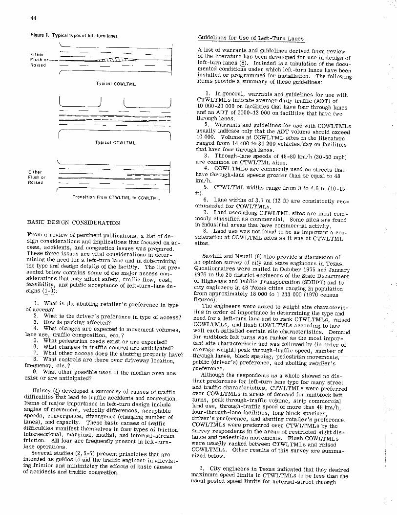
44
Figure 1. Typical types of left.turn lanes.
BASIC DESIGN CONSIDERATION
From a review of pertinent publications, a list of de_sign considerations and implications that focused on ac_cess, accidents, and congestion issues was prepared,These three issues are vital considerations in deter_mining the need for a left-turn lane and in determiningthe type and design details of the facility. The list prã_sented below contains some of the major access con_siderat_i.ons that may affect safety, traffic flow, eost,feasibility, and public acceptance of left-turn-lane de_signs (1-3):
1. What is the abutting retailerrs preference in typeof access?
2. What is the driverrs preference in type of access?3. How is parking affected?4, What changes are expected in movement volumes,
lane use, traffic composition, etc. ?
?. What pedestrian needs exist or are e¡pected?I. What changes in traffic control are anîicipated?
G.ridelines for Use of Left-Turn Lanes
A list of warrants and guidelines derived from review
left-turn lanes (8). Included is a tabulation of the docu_mented condition-s under which left-turn lanes have beeninstalled or programmed for installation, The followingitems provide a summary of these guidelinesl
1, In general, warrants and guidelines for use withCTWLTMLs indicate average daily traffic (ADT) of10 000-20 000 on facilities that have four through lanesand an ADT of 5000-12 000 on facilities that have twothrough lanes,
2, Warrants and guidelines for use with COWLTMLsusually indicate only that the ADT volume should exceed10 000. Volumes at COWLTML sites in the literatureranged from 14 400 to B1 200 vehicles/day on facilitiesthat have four through lanes.
3. Through-lane speeds of 48-80 kmlh (80_bO mph)are common on CTWLTML sites,
4. COWLTMLs are commonly used on streets thathave through-lane speeds greater than or equal to 48km/h.
5. CTWLTML widths range from B to 4.6 m (10-1bfÐ.
6. Lane widths of J.T m (12 ft) are consistenfly rec_ommended for COWLTMLs.
1. Land uses atong CTWLTML sites are most com_monly classified as commercial, Some sites are foundin industrial areas that have commercial activity.L Land use was not found to be as importani a con_sideration at COWLTML sites as it \,vas al CfWf,flvIf,sites.
Sawhill and Neuzil (8) also provide a discussion ofan opinion survey of ciFy and state engineers in Texas,Questionnaires were mailed in October lg?b and January1976 to the 25 district engineers of the State Departmeniof Highways and Public Transportation (SDHpTf and tocity engineers in 48 Texas cities ranging in populationfrom approximatety 1B 000 to 1 233 O-00 119?õ censusfigures),
The engineers were asked to weight site characteris_tics_in order,of importance in determining the þpe andneed for a left-turn lane and to rank CTWLTMLS-, raisedCOWLTMLs, and fIush COWLTMLs according to howwell each satisfied certain site characteristics. Demandfor midblock left turns was ranked as the most impor_tant site characteristic and was followed by (in order of
Typicol COWLTML
lt
EitherFlush orRo ¡ sed
ai/erage weight) peak through-traJfic speed, number of
TypicolCTWLTML
ïronsition From CTWLTML to COWLTML
1. What other8. What controls are there over driveway licaiion,
frequency, etc. ?9. What other possible uses of the median area now
exist or are anticipated?
Halsey (4) developed a summary of causes of trafficdifficultiesÏhat lead to tra.ffic acciãents and congestion.Items of major importance in left-turn design includeangle"s of movement, velocity differences, icceptablespeeds, convergence, divergence (changing number oflanes), and capacity. These basic causès ãf hafficdifficulties manifest themselves in four types of friction:intersectional, marginal, medial, and iniðrnal-streamfriction. All four are frequenily present in left-turn-lane operations,
. Several studies (Z,Z-! present principles that areintended as guides tõ afd-ttre traffic enginãer in alleviat_ing friction and minimizing the effects of basic causesof accidents and traffic congestion.
public (driver's) preference, and abutting retailer?spreference.
Although the respondents as a whole showed no dis_tinct preference for left-turn lane type for many streetand traffic characteristics, CTWLTMLs were preferredover COWLTMLs in areas of demand for midblbck leftturns, peak through-traffic volume, strip commercialland use, through-traffic speed of more lhan 48 km/tr,four-through-lane facilities, Iong block spacings,{!y9r's preference, and abutting retailei's prãfórence.COWLTMLs were preferred over CTWLTMis by thesurvey respondents in the areas of restricted sight dis_tance and pedestrian movements. Flush COWLTMLswere usually ranked between CTWLTMLs and raisedCOWLTMLs. Other results of this survey are summa-rized below.
1. City engineers in Texas indicated that they desiredmaximum speed limits in CTWLTMLs to be less than theuzual posted speed limits for arterial-street through
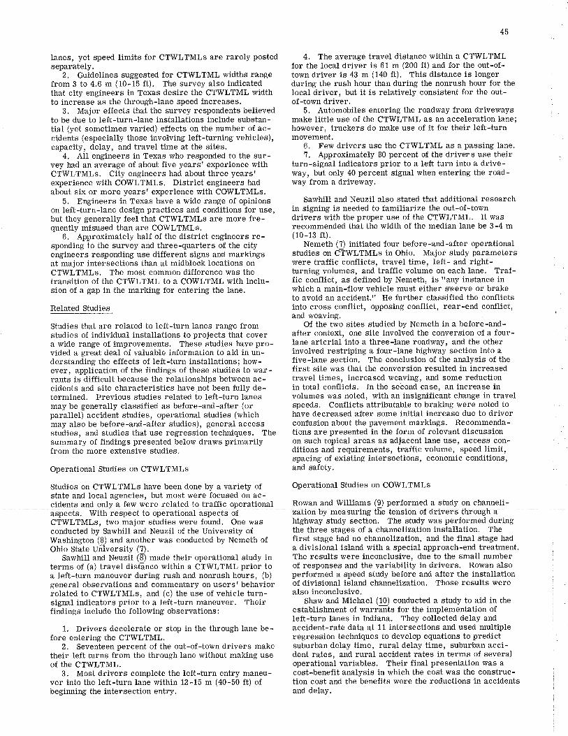
Ianes, yet speed limits for CTWLTMLs are rarely postedseparately.
2. Guidelines suggested for CTTtrLTML widths range
45
4. The average travel distance within a CTWLTMLfor the local driver is 61 m (200 ft) and for the out-of-town driver is 43 m (140 ft). This distance is longer
Irom ó Io +,o m (ru-ro rt,r. Ine sul'vey alsu ¡IlqluaLcqthat city engineers in Texas desire the CTWLTML widthto increase as the through-lane speed increases.
3. Major effeets that the survey respondents believedto be due to left-turn-lane installations include substan-tial (yet sometimes varied) effects on the number of ac-cidents (especially those involving left-turning vehicles),capacity, delay, and travel time at the sites.
4. AII engineers in Texas who responded to the sur-vey had an average of about five years' experience withCTWLTMLs. City engineers had about three years'e4perience with COWLTMLs. District engineers hadabout six or more yearsr e4perience with COWLTMLS.
5, Engineers in Texas have a wide range of opinionson left-turn-Iane design practices and conditions fot use,but they generally feel that CTWLTMLS are more fre-quently misused than are COWLTMLS.
6. Approximately half of the district engineers re-sponding to the survey and three-quarters of the cityengineers responding use different signs and markingsat major intersections than at midblock locations onCTWLTMLs. The most common difference was thetransition of the CTWLTML to a COWLTML with inclu-sion of a gap in the marking for entering the lane.
Related Studies
Studies that are related to left-turn lanes range fromstudies of individual installations to projects that covera wide range of improvements. These studies have pro-vided a great deal of valuable information to aid in un-derstanding the effects of left-turn installations; how-ever, application of the findings of these studies to war-rants is difficult because the relationships between ac-cidents and site characteristics have.not been fully de-termined, Previous studies related to left-turn lanesmay be generally classified as before-and-after (orparallel) accident studies, operational studies (whichmay also be before-and-after studies), general accessstudies, and studies that use regression techniques, Thesummary of findings presented below draws primarilyfrom the more extensive studies.
Operational Studies on CTIVLTMLs
Studies on CTIVLTMLs have been done by a variety ofstate and local agencies, but most were focused on ac-cidents and only a few were related to traffic operational Rowan and Williams (9) performed a study on channeli-aspects, With respect to operational aspectsCTWLTMLs, two major studies were found. One wasconducted by Sawhill and Neuzil of the University of
qurlng f,Ile rusrr rruul Lrtil,rr qufurB, Lllg rrurrfusll lluul rul' Lrlu
Iocal driver, but it is relatively consistent for the out-of-town driver,
5. Automobiles entering the roadway from drivewaysmake little use of the CTWLTML as an acceleration lane;however, truckers do make use of it for their left-turnmovement.
6. Few drivers use the CTWLTML as a passing lane.1. Approximately 80 percent of the drivers use theil
turn-signal indicators prior to a left turn into a drive-way, but only 40 percent signal when entering the road-way from a driveway.
Sawhill and Neuzil also stated that additional researchin signing is needed to familiarize the out-of-towndrivers with the proper use of the CTWLTML. It wasrecommended that the width of the median lane be 3-4 m(10-13 fr).
Nemeth (7) initiated four before-and-after operationalstudies on CTWLTMLs in Ohio. Major study parameterswere traffic conflicts, travel time, left- and right-furning volumes, and traffic volume on each lane, Traf-fic conflict, as defined by Nemeth, is t'any instance inwhich a main-flow vehicle must either swerve or braketo avoid an accident," He further classified the conflictsinto cross conflict, opposing conflict, rear-end conflict,and weaving.
Of the two sites studied by Nemeth in a before-and-after context, one site involved the conversion of a four-lane arterial into a three-lane roadway, and the otherinvolved restriping a four-lane highway section into afive-lane section. The conclusion of the analysis of thefirst site was that the conversion resulted in increasedtravel times, increased weaving, and some reductionin total conflicts. In the second case, an increase involumes was noted, with an insignificant change in travelspeeds. Conflicts attributable to braking were noted tohave decreased after some initial increase due to driverconfusion about the pavement markings, Recommenda-tions are presented in the form of relevant discussionon such topical areas as adjacent lane use, access con-ditions and requirements, traffic volume, speed limit,spacing of existing intersections, economic conditions,and safety.
Operational Studies on COWLTMLS
highway study section. The study was performed duringthe three stages of a channelization installation. The
luashington (B) and another was conducted by Nemeth of first stage had no channelization, and the final stage had
Ohio State Uñiversity (?). a divisional island with a special approach-end treatment.Sawhill and Neuzil (8) made their operational study in The results were inconclusive, due to the small number
terms of (a) travel distãnce within a CTWLTML prior to of responses and the variability in drivers. Rowan alsoa left-turn maneuver during rush and nonrush hours, (b) performed a speed study before and after the installationgeneral observations and commentary on users'behavior of divisional island channelization. Those results wererelated to CTWLTMLs, and (c) the use of vehicle turn- also inconclusive.signal indicators prior to a left-turn maneuver. Their Shaw and Michael (10) conducted a study to aid in thetiñOings include tñe following observations¡ €stablishment of warrã-nts for the implementation of
left-turn lanes in Indiana. They collected delay and1. Drivers decelerate or stop in the through lane be- accident-rate data at 11 intersections and used multiple
fore entering the CTWLTML. regression techniques to develop equations to predÍct2. Seventeen percent of the out-of-town drivers make suburban delay time, rural delay time, suburban acci-
their left turns from the through lane without making use dent rates, and rural accident rates in terms of severalof the CTWLTML. operational variables. Their final presentation was a
3. Most drivers complete the teft-turn entry maneu- cost-benefit analysis in which the cost was the construc-ver into the left-turn lane within 12-15 m (40-50 ft) of tion cost and the benefits were the reductions in accidentsbeginning the intersection entry. and delay.
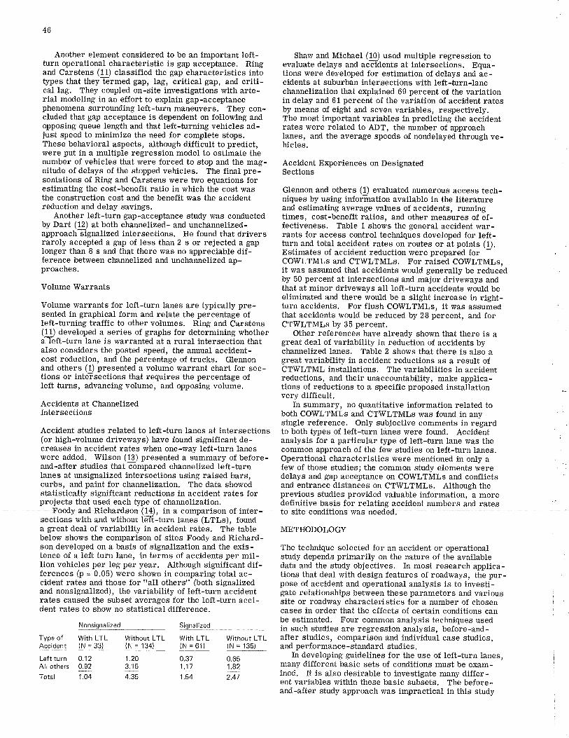
46
Another element considered to be an important left-turn operational characteristic is gap acceptance. Ring
Shaw and Michael (10) used multiple regression toevaluate delays and aiõÏdents at intersections. Equa-tions were developed for estimation of delays and ac-and Carstens (11) classified the gap characteristics into
Þ*rt 'EÞtcal lag. They coupled on-site investÍgatíons with arte-rial modeling in an effort to explain gap-acceptancephenomena surrounding left-turn maneuvers. They con-cluded that gap acceptance is dependent on following andopposing queue length and that left-turning vehicles ad-just speed to minimize the need for complete stops.These behavioral aspects, although difficult to predict,were put in a multiple regression model to estimate thenumber of vehicles that were forced to stop and the mag-nitude of delays of the stopped vehicles. The final pre-sentations of Ring and Carstens were two equations forestimating the cost-benefit ratio in which the cost wasthe construction cost and the benefit was the accidentreduction and delay savings.
Another left-turn gap-acceptance study was conductedby Dart (12) at both channelized- and unchannelized-approach-Signalized intersections. He found that driversrarely accepted a gap of less than 2 s or rejected a gaplonger than 8 s and that there was no appreciable dif-ference between channelized and unchannelized ap-proaches.
Volume Warrants
Volume warrants for left-turn lanes are typically pre-sented in graphical form and relate the percentage ofleft-turning traffic to other volumes. Ring and Carstens(11) developed a series of graphs for determining whethera left-turn lane is warranted at a rural intersection thatalso considers the posted speed, the annual accident-cost reduction, and the percentage of trucks, Glennonand others (1) presented a volume warrant chart for sec-tions or inteisections that requires the percentage ofleft turns, advancing volume, and opposing volume.
Accidents at ChannelizedIntersections
Accident studies related to left-turn lanes at intersections(or high-volume driveways) have found significant de-creases in accident rates when one-way left-turn laneswere added. Wilson (13) presented a summary of before-and-after studies thatlõmpared channelized left-turnIanes at unsignalized intersections using raised bars,curbs, and paint for channelization, The data showedstatistically significant reductions in accident rates forprojeets that used each type of channelization.
@dsections with and without left-turn lanes (LTLs), founda great deal of variability in accident rates. The tablebelow shows the comparison of sites Foody and Richard-son developed on a basis of signalization and the exis-tence of a left turn lane, in terms of accidents per mil-lion vehicles per leg per year. Although significant dif-ferences (p = 0.05) were shown in comparing total ac-cident rates and those for "all others'1 (both signalizedand nonsignalized), the variability of left-turn accÍdentrates caused the subset averages for the left-turn acci-dent rates to show no statistical difference.
Nonsignal ized Signalized
channelization that e4plained 69 percent of the variationin delay and 61 percent of the variation of accident ratesby means of eight a¡d seven variables, respectively.The most important variables in predicting the accidentrates were related to ADT, the number of approachlanes, and the average speeds of nondelayed through ve-hicles.
Accident Experiences on DesignatedSections
Glennon and others (1) evaluated numerous aceess tech-niques by using inforhation available in the literatureand estimating average values of accidents, runningtimes, cost-benefit ratios, and other measures of ef-fectiveness. Table 1 shows the general accident war-rants for access control techniques developed for left-turn and total accident rates on routes or at points (1).Estimates of accident reduction were prepared for -COWLTMLS and CTWLTMLs. For raised COWLTMLs,it was assumed that accidents would generally be reducedby 50 percent at intersections and major driveways andthat at minor driveways all left-turn accidents would beeliminated and there would be a slight increase in right-turn accidents, For flush COrt¡/LTMLs, it was assumedthat accidents would be reduced by 28 percent, and forCTWLTMLS by 35 percent.
Other references have already shown that there is agreat deal of variability in reduction of accidents bychannelized lanes. Table 2 shows that there is also agreat variability in accident reductions as a result ofCTWLTML installations. The variabilities in accidentreductions, and their unaccountability, make applica-tions of reductions to a specific proposed installationvery difficult.
In summary, no quantitative information related toboth COWLTMLs and CTWLTMLs was found in anysingle reference, Only subjective comments in regardto both types of left-turn lànes were found. Accidentanalysis fìr a particular type of left-turn lane was thecommon approach of the few studies on left-turn lanes,Operational characteristics were mentioned in only afew of those studies; the common study elements weredelays and gap acceptance on COWLTMLs and conflictsand entrance distances on CTWLTMLs. Although theprevious studies provided valuable information, a moredefinitive basis for relating accident numbers and rates i'to sitssondÍtions- warnqsd
METHODOLOGY
The technique selected for an accident or operationalstudy depends primarily on the nature of the availabledata and the study objectives. In most research apptica-tions that deal with design features of roadways, the pur-pose of accident and operational analysis is to investi-gate relationships between these parameters and varioussite or roadway characteristics for a number of chosencases in order that the effects of certain conditions canbe estimated. Four common analysis techniques usedin such studies are regression analysis, before-and-after studies, comparison and individual case studies,and perf ormance - standard studies.
In developing guidelines for the use of left-turn lanes,many different basic sets of conditions must be exam-ined. It is also desirable to investigate many differ-ent variables within these basic subsets. The before-and-after study approach was impractical in this study
Type of With LTLAccident 1N = 33)
Left turn 0.12All others O.92
Total 1.O4
Without LTL With LTL(N = 134) (N = 6f)
1.203.15
4.35
Without LTL(N = 135)
0.371.'t7
1.54
0.651.82
2.47
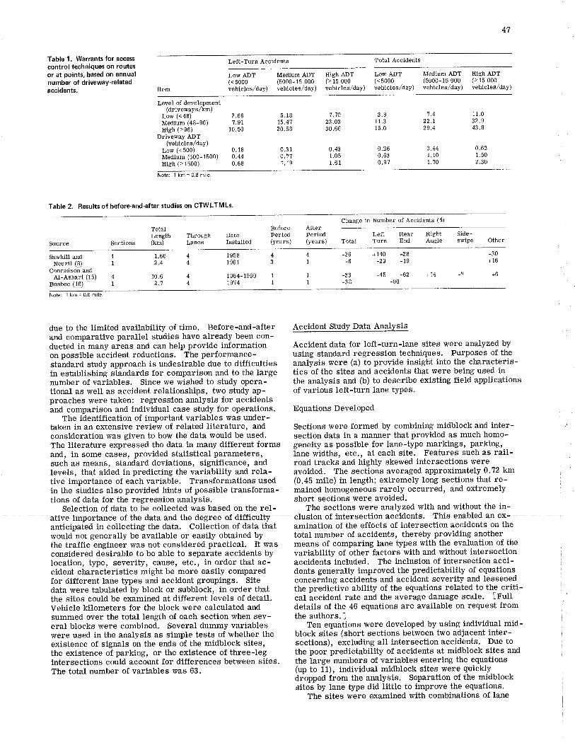
47
Table 1. Warrants for access
control techniques on routesor at points, based on annualnumber of driveway-relstedaccidents.
Left-Turn Accidents Total Accidents
Low ADT Medium A.DT High ADT(<5000 (5ooo-15 000 (>15 000vehicles/day) vehicles/day) vehicles/day)
Low A.DT Medium ADT High ADT(.5000 (5000-15 000 (>15 000vehicles/day) vehicles/day) vehicles/day)
Level of development(driveways/km)
Low (<48)Medium (48-96)Hieh (>96)
Driveway ADT(vehicles/day)
Low (<500)Medium (500-1500)Hieh (> 1500)
2.66?.91
10.50
0.180.440.68
5.1815.4120.58
0.310.711.19
0.441.101. ?0
7.7023.0330.66
0.431.051.61
3.8I 1.3t5,0
0.260.630.9?
1,422.t29.4
I 1.032.943.8
0.621.502.30
Note: 1 km = 0.6 mile.
Table 2. Results of before-and"after studies on CTWLTMLS.
Change in Number of Accidents (ß)
TotaILength Through
Sections (km) Lanes
Before AfterPeriod Period(years) (years)
DateInstalled
Side-swipe Other
LeftTotal Turn
Rear RightEnd AngieSource
Sawhill and INeuzil (8) 1
Conradson- andAl-Ashari (15) 4
Busbee (16) - 1
+140 -28-25 -19
-45 -62-90
tions of data for the regression analysis.Selection of data to be collected was based on the rel-
41
1
1
short sections were avoided.The sections were analyzed with and withot¡t the in-
1.662.4
10.6
-26-6
-33-38
-30+16
+14 -7 +6
43
1
I
19581961
44
44
1964-19691974
ffi; 1 k. = os.¡le
-L
due to the limited availabiliW of time. Before-and-after Accident Study Data Analysisand comparativeparallel studieshavealreadybeencon-
-
:
ducted in many aieas and can help provide inÍormation Accident data for left-turn-lane sites were analyzed by
on possible accident reductions. -The performance- using standard regression techniques' Purposes of the
sta-ndard study approach is undesirablè due to difficulties analysis were (a) to provide insight into the characteris-in establishing s-tandards for comparison and to the large tics of the sites and accidents that were being used innumber of variables. Since we wished to study opera- the analysis and (b) to describe existing field applicationstional as well as accident relationships, two study ap- of various left-turn lane types.proaches were taken: regression analysis for accidentsãnd comparison and individual case study for operations. Equations Developed
The identification of important variables was under-taken in an extensive review of related literature, and Sections were formed by combining midblock and inter-consideration was given to how the data would be used. section data in a manner that provided as much homo-The literature expressed the data in many different forms geneiff as possible for lane-type markings' parking'and, in some cases, provided statistical parameters, lane widths, etc,, at each site, Features such as rail-such as means, standard deviations, significance, and road tracks and highly skewed intersections wereIevels, that aided in predicting the variability and rela- avoided. The sections averaged approximately 0'?2 km
I
tive importance of each variable. Transformations used (0.45 mile) in length; extremely long sections that re-in the studies also provided hints of possible transforma- mained homogeneãus rarely o."u""õd, and extremely
@1hêlata andllle degree of difficult-y cluEiorof-i¡tersection-¿ccidents. Thisenabledan ex.anticipatled in collecting the data. Co[èction of data that amination of the effects of intersection accidents on the
would not generally be ãvailable or easily obtained by total number of accidents, thereby providing anotherthe trafficlngineer was not considered practical. It was means of comparing lane types with the evaluation of the
considered desirable to be able to separãte accidents by variability of other factors with and without intersectionlocation, type, severity, cause, etc., in order that ac- accidents included. The inclusion of intersection acci-cident ciraiácteristics might ¡e more easily compared dents generally improved the predictability of equationsfor different lane types and accident groupings. Site concerning accidents and,accident severity and le,ssened
data were tabulatedby block or subbtãck,- inìrder that the predictive ability of the equations related to the criti-the sites could be examined at different levels of detail. cal àccident rate and the average damage scale. lFutlVehicle kilometers for the block were calculated and details of the 46 equations are available on request fromsummed over the total length of each section when sev- the authors. leral blocks were combined. Several dummy variables Ten equations were developed by using_ individual mid-were used in the analysis as simple tests oi whether the block sites (short sections between two adjacent inter-existence of signals on the ends õf the midblock sites, sections), excluding all intersection accidents. Due to
the existence oi parking, or the existence of three-Ieg the poor predictability of ac,cidents at midblock sites and
intersections could accõunt for differences between sites. the large numbers of variables entering the equations
The total number of variables was 63. (up to 11), individual midblock sites were quicklydropped from the analysis. Separation of the midblocksites by lane type did little to improve the equations'
The sites were examined with combinations of lane
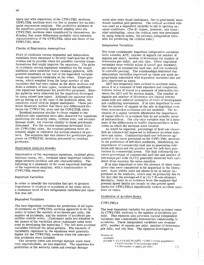
scale also were found inadequate, due to previously men-tioned residual plot patterns. The critical accident ratewas used as a dependent variable to aid in spotting un-uzual conditions. (The R2 values, however, ate so¡ne-what misleading, since the critical rate was developedby using vehicle miles, the primary independent vaii-airte tor predicting the'critical rate,)
Independent Variables
The most consistently important independent variableswere weekday ADT, number of signals (or number ofsignals per mile), number of driveways (or number ofdriveways per mile), and city size. Other importantvariables were vehicle miles of travel (per weekday),percentage of commercial land use, and the existenceof curbside parking. The relationships indicated thatindependent variables expressed as rates are most ap-propriately associated with dependent variables that arealso ex¡lressed as rates,
ADT has frequently been related to accident rates,since it is a measure of both exposure and congestion,Vehicle miles of travel is a measure of interaction be-tween the ADT and the section length. The number ofsignals and number of driveways are logical entriessince both are indirect measures of level of developmentand conflicting movements, It is also important to notethat the number of signals on the site is important evenwhen intersection accidents are not included, The in-clusion of a signal variable illustrates the importanceof signal effects on accidents that do not actuálly occurat intersections. The city-size variable may be a mea-sure of the differences in traffic characteristics of thecities in which the sections were located.
As might be e>ipected, percentage of land use classi-fied as commercial appeared to infl.uence accident num-bers and rates, Commercial-Iand-use influences ap-peared to be more prevalent on the CTWLTML sectionsin the prediction of left-turn accidents, illustrating theimportance of .commercial land use in generating mid-block left turns and the greater need for left-turn pro-visions in commercial areas, The high colinearity be-tween percentage of commercial land use and number ofdriveways per mile (0.6?1) generally deterred both vari-ables from entering the same equation,
It is also important to note the absence of other vari-ables that were considered to be important in the litera-ture, Lane widths were not shown to be of major im-portance in the analysis, which may be primarily due tothe fact that the average-3.6 m (11.7 ft)-is adequate.Similarly, there is no evidence from the analysis that
lrrorderto identify thevariablertffi areofgreatest present speed limits arsr¡nsaCercr that posted speedimportance in relation to accidents at the study sites, limits for CTWLTMLs significantly reduce accident num-a maximum level of five independent variables per equa- bers or rates.tion was set,
Prediction of Accident RatesDependent Variables
The best dependent variables for prediction of all typesof accidents on CTWLTML sections appeared to be (inorder of value) the number of accidents per mile, thenumber of accidents, a4d the number of accidents permillion vehicle miles. lCustomary units are retained inthe names of the variables since customary units wereused in developing the equations. I the left-turn accidentvariables followed the same pattern. The amounts ofvariability e>çlained by the equations were generallyhigher for the CTWLTML sections when the intersec-tion accidents were included.
The severity index and average damage scale werevery unpredictable, as was expected. The equations forprediction of the severity index and average damage
48
types and with separation of the CT\ryLTML sections.COWLTML sections were too few in number for an ade-quate regression analysis. The predictive abilities ofthe equations generally improved slightly when theCT\ryLTML sections were considered by themselves, in-dicating that some differences probably exist betweencharacteristics of the CTWLTML sites and those of theCOWLTML sites.
Checks of Regression Assumptions
Plots of residuals versus dependent and independentvariables were examined to identify inadequacies of themodels and to provide clues for possible variable trans-formations that might improve the equations. The plotsof residuals versus dependent variables for the singlemidblock sites exhibited linear residual patterns, withpositive residuals on one end of the dependent variablerange and negative residuals on the other. These pat-terns, which resulted from the large number of sitevariables that had zero values on the short sections andfrom a mixture of lane types, rendered the midblock-site equations inadequate for predictive purposes. Simi-lar patterns were observed for the equations developedby using mixed lane types. Although the patterns werenot as strong as in the case of the midblock sites, theequations would still be judged inadequate. These pat-terns illustrate further that there are differences be-tween the CTWLTML sites and the COWLTML sites.
Residual patterns similar to those related to themidblock-site equations were also observed for equationspredicting the severity index, critical rate, and averagedamage scale, for reasons similar to those prevÍouslydiscussed, For the section equations developed fromthe CTWLTML sites, the residual patterns were ex-tremely slight or exhibited the normal absence of pat-tern. The equation that was chosen for predictive pur-poses on CTWLTML sections presented no residualproblems.
Regression Analysis Results
Examination of the regression equations, residual plots,extreme cases, etc., revealed many important relation-ships between accident and site characteristics. Thefollowing is a summary of the most important findingsof the regression analysis, with a concentration onCTWLTML equations.
Important Variables
CTWLTMLS
The best dependent variable for predicting accident rateson CTWLTML sections is the number of accidents permile. This equation also provides logical independentvariables that consistently demonstrate relationship toaccidents, These independent variables are weekdayADT, number of signals per mile, number of drivewaysper mile, and city size. The equation developed is
Number ofaccidentsper mile = -43.5 + 0.002 03(ADT) + 0.000 175 (city population)
+ 0.491 (number of driveways per mile)+ 9.2fJ (number of signals per mile) (l)
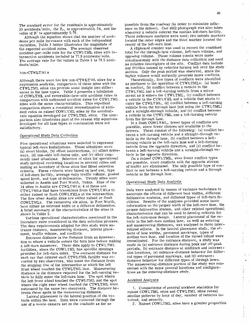
49
The standard error for the residuals is approximately possible from the roadway (in order to minimize influ-33 accidents/mile, the F,"g is approximat-e-þ 34, and ihe ence on the driver)' One still photograph was also taken
,áf"ã ãlntis appíoximatrif' O.iå. whenever a vehicle entered the median left-turn facility'Although
dents per mile inôreases with each of the independent located the outer edges and the third marker located the
variables, Table 3 better illustrates the magnitude of center of the left-turn lane.the elçecied accident rates. The average observed A clipboard counter was used to record the combined
accident-per-mile rate for the CTWLTùL sites with in- total for the through-lane volume, Ieft-turn volume, and
tersectioñ accidents included is ??.9 accidents/mile. opposing volume.. .These volume counts were made
The average rate for the values in Table 3 is ?9.5 acci- simultaneously with the distance data collection and used
Jé"t"/-ii"i. as relative descriptors of the site. Conflict data includeany friction caused by vehicles turning left over the study
N.'-CTWLTML5 "eätion. OnIy the peak period was observed, since the
higher volume would normally generate more confl'icts'
Although there were too few non-CTWLTML sites for a Theoretically, five types of conflicts were identified .reg"esiion analysis, comparison of these sites with the as pertinent to the operation of CTWLTMLs: (a) head-
CTWLTML siteä caí p"ovìde some insight into differ- on õonflict, (b) conflict between a vehicle in the
ences in the lane types. Table 4 presents a tabulation CTWLTML and a left-turning vehicle from a minorof COWLTML and reversible-Iane-site accident rates in street as it enters the CTWLTML, (c) conflict between
comparison with estimated accident rates for CTWLTML a vehicle in the CTÏ|¡LTML and a vehicle that starts tositeà with the same characteristics. This expedient enter the CTWLTML, (d) conflict between a left-turning ù
comparison shows a consistent overestimation of acci- vehicle from the through lane (not using the CTWLTML)dent rates on raised COWLTML sites by the accident- and a straight-through vehicle, and (e) conflict between
rate equation developed for CTWLTML sites. The com- a vehicle in the CTWLTML and a left-turning vehicleparison also illustrates part of the reason why equations from the through lane'äeveloped for all lane tyþes in combination were not In a flush COWLTML, fewer types.of .conflicts are
satisfactory. possible, since fewer choices are available to theãrivers. These consist of the following: (a) conflict be-
Operational Study Data Collection tween a left-turning vehicle and a straight-through ve-hicle in the through lane, (b) conflict between a left-
Five operational situations were selected to represent turning vehicle in the left-turn lane and a left-turningtypicaf left-turn installations. These situations were vehiclã from the opposite direction, a$-(c) conflict be-(äj short blocks, (b) offset intersections, (c) offset drive- tween a left-turning vehicle and a straight-through ve-ways, (d) one-side left-turns only, and (e) other com- hicle in the opposite direction'monfí use¿ situations. Selection of sites for operational On a raised COWLTML, even fewer conflict types
study involved reviewing locations in several cities and are possible, since conflicts with the opposite stream
maklng an inventory of those sites that fitted selection of trãffic are eliminated. The only possible type of con-
criteria, These criteria were based on land use, type flict is one between a left-turning vehicle and a throughof left-turn facility, average daily traffic volume, posted vehicle in the through lane.speed limit, and type of delineation. Twenty sites weresèlected in Austin ánd Fort Worth, Texas. Nine of the Operational Study Data Analysis14 sites in Austin are CTWLTMLs; 4 of these arecTwLTMLs that have transitions from cTWLTMLs to Data were analyzed by means of variance techniques to
either raised or flush COWLTMLs at the intersection. ascertain the effects of different lane widths, differentThe five other Austin sites are either raised or flush delineation systems, and different types of left-turn fa-COWLTMLs. The remaining six sites, in Fort Worth, cilities. Results of the analyses provided some basic
have either an extreme width or a different delineation. information on the proper width of the left-turn lane, the
A brief s.r*-""y of the characteristics of the sites is proper delineation system, and other re.Iated operationalshown in Table b. õharacteristics that can be used to develop criteria for
Various operational characteristics mentioned in the the left-turn-lane design. Lateral placement of the ve-Iiterature welre considered in the data selection process. hicle in the left-turn median lane, as well as entering
asauatY zedin thre rinter -trance distance, *anerrver-ing distance, lateral place- related efforts. In the lateral placement study, the ef-ment, traffic .1ró1o*", and co-nflicts. fects of lane widths, pavement markings, types of
Entrance distance is the distance from an intersec- median turn lane, and location of the raised island were
tion to where a vehicle enters the turn lane before making investigated. For the entrance distance, a study was
a left-turn maneuver. These data apply to CTWLTML made on (a) entrance distance during peak and off-peak
facilities, since the COWLTML hasþðcific openings periods, (b) entrance dista¡ce at midblock and intersec-provided for left-turn entry. The entiance diÃtance for tion locations, (c) entrance-distance behavior for differ-each car that entered each CTWLTML facility was re- ent types of pavement markings' and (d)
-entrance-corded by two observers, who noted the distance from distance behavior for different types of through lanes.
the stopplng line of the iátersection at which the left The maneuvering-distance portion of the study was con-
front wheel touched the CTWLTML line. Maneuvering cerned with the same general locations and configura-
distance is the distance required for the left-turning ve- tions as the entering-distance study'
hicle to fuIIy enter the left-turn lane' The spot wherethe left front wheel touched the CTWLTML and the spotwhere the right rear wheel touched the CTWLTML wereestimated by the same two observers. The distance be-tween these spots is the maneuvering distance.
Lateral placement is the lateral position of the ve-hicle within the lane. Data were collected through theuse of a movie camera set on the roadside as far as
Accident Analyses
1, Comparisons of general accident statistics forraised COWLTML sites and CTWLTML sites revealsimilar patterns by hour of day, number of vehicles in-volved, and severitY,
2. Raised COWLTML sites have a greater proportion
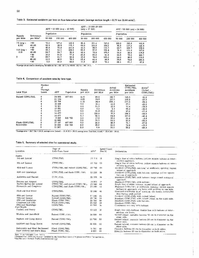
50
Table 3. Est¡mated accidents per lane on four-lane urban streets [average section length = 0.71 km (0.44 mile]].
ADT = 15 000-20 000uvw \4Yó - ¡v ¿:u/ (¿vts = rr uuu, PL. -¿v uuu (avg = z{ ÐUU)
Population Population PopulationStg¡als Drivewaysper Mile per Mile' 50 000 250 000 400 000 50 000 250 000 400 000 50 000 250 000 400 000
>3 (avg = >604.63) 40-60
<û1-3 (avg = >60
2,0) 410-60<û
0 >60ItO-60<,40
72.353.940.448.129,716.229.111.30.0
10?.388.975,483.164.161.264,146.332.8
133.5115.1101.6109.390.9,t7.4
90.972.559.0
86.468.054.562.243.830.843.825.41 1.9
127.4103.089.591.278.865.378.860.446.9
147.6129.2t15.1123.4105.091.5
105.086.6?3.1
100.6 135.6 161.882.2 171 .2 143 .468.? 103.? 129.516.4 111.4 13?.658.0 93.0 t19.244.5 ?9.5 105.?58.0 93.0 119.239.6 74.6 100.826.7 61.1 8?.3
'Averag€valuesusd¡ndevelop¡ngthetablearefor>60: 87.7;for4G60: 50l.for<4Ot 22.7,
Table 4. Comparison of acc¡dent rates by lane type.
NumberofThrough
Lare Type LanesSignals
Population per Mile
ActualDriveways Accidentsper Mile per MileAÐT
EstimatedCTWLTMLAccidentsper Mile
Error(Actual -CTWLTML)
Ralsed COWLTML 40? 000 4.114.653.130.00.00.00.00.02.7
283 ?00 0.03.2
40? 000 0.0283 ?00 2.0
2.9
Flush COWLTMLReversible
66644444
46422
29 56231 13432 ?0615 48313 92113 591t4 47174 41174 471I 323
13 66017 t9?13 22311 367
39.639.584.416.13 1.30.0
81.8100.062,51?.03 5.523.356,0
5.9
166.?721.9253.141.9t2.59.4
65.9?6.364.936.229.046.466.03 5.3
145.6153.23 1?.5
67.171.455.49?.3
106.310?.031.481.014.178.959.2
+27.2-25.3-64.4-25.2-58, I-46.0-31.4-30.0-42.4+4,8
-52.0-27.6-t2.9-23.9
'Ave/agè error = 29,7 (SD = 24.3); average error (raisd) = -31.8 (SD = 26.1 ); average error (four-lane. rahed) = -33.4 (SD = 20.3)
Table 5. Summary of selected s¡tes for operational study.
LocationType ofLeft-Turn Lane
Speed LimitADT' (km/h) Delineation
Austin5th and Lamar
6th and Lamãr
45th and Lamar
4ãth and Guadalupe
Anderson and Burnet
CTWLTML
CTWLTML
CTWLTML and raised COWLTML
CTWLTML and flush COWLTML
CTWLTML
31 110 56
31 110 56
25 ?80 64
23 2t0 56
22 '',t0
64
Single line of white buttons; yellow square buttons at inter-section approach.
Single line of white buttons: yellow square buttons at inter-section approach.
Standard CTWLTML markingb at midblock; opening; raisedisland at approach.
Standard CTWLTML with buttonsi opening; yellow squarebuttons at approach.
Stân.lâr.i ÍìTWI.TMT. with h¡ft¡nc. lâroê ¡^,,nd hr#^ñê ol
Denson and AirportBarton SÞring and LamarRiverside and Congress
32rd and Red River
45th and Lamar19th and Lamar45th and GradalupeCongress and 1gth26th and Gradalupe
FoÌt WorthCockell and Berry
Wichita and Mansfield
Bigham and Camp Bowie
Guliford and Camp Bowie
University and West SettlementEâst Vickery and South Main
CTWLTMLCTWLTML and raised COWLTMLCTWLTML and flush COWLTML
CTWLTML
Raised COWLTMLRaised COWLTMLFlush COTVLTMLFlush COWLTMLCOWLTML
CTWLTML
Raised COWLTML
Raised COWLTML
Raised COWLTML
Flush COWLTMLFlush COWLTML
19 06029 94027 340
t2 240
21 68025 79020 73025 04026 980
19 500
14 500
28 ?00
32 200
't2
56
48
6456564856
56
64
56
56
approach.Standard CT\Í/LTML with buttons.Single Line of white buttons; raised island at approach.Standard CTWLTML at midblocki opening; yellow square
buttons at approach; six lanes with parking on one side.Standard reversible laneb marking; two lanes; reversible
lane during peak period.Standard COWLTML with raised island.Standard COWLTML with raised island on the right side.Standard COWLTML with buttons.Standard COWLTML.Continuous one-wav with buttons.
Single line with buttonst double line with buttons at inter-section; six lanes.
Raised island; metâllic buttons 30 cm in diameter on theother side.
Raised islandl ceramic buttons 20 cm in diameter on theother side.
Raised island; ceramic buttons 20 cm in diameter on theother side.
Ceramic buttons 20 cm in diameter on both sides.Metallic buttons 30 cm in diameter on both sides.
16 ?00 48I 000 48
Note: 1 km = 0,6 m¡le; 1 cm = 0,4 in"Obtained from 'l 975 volume count furn¡shed by the Texas Department of H¡ghways and Publ¡c Transportation.bSee Manual on Un¡fornì Traffic Control Devices (17).
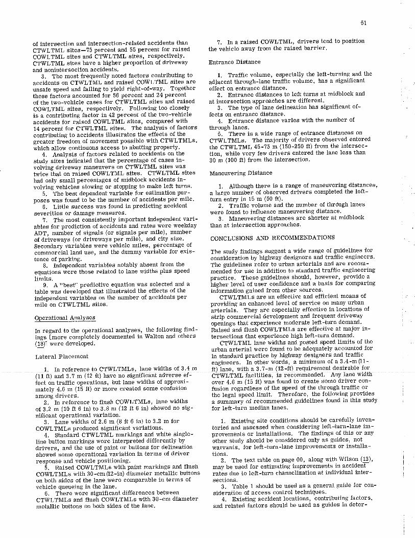
COWLTML sites and CTWLTML sites, respectively'CTïI¡LTML sites have a higher proportion of driveway Entrance Distanceand nonintersection accidents'
B. The most frequenUy noted factors contributing to 1. Traffic volume, especially the left-turning and the
accidents on CTWLTML and raised CO\ryLTML sites are adjacent through-lane traffic volume, has a significantunsafe speed and failing to yield right-of-way' Together effect on entrance distance'these faõtors accounteal- for-56 percent and 24 percent 2. Entrance distances to left turns at midblock and
of the two-vehicle cases for CiWf,fUL sites and raised at intersection approaches are different'CO'ffLTML sites, respectively. Following too closely 3. The type of lane delineation has significant ef-is a contributing factor in 42 percent of the two-vehicle fects on entrance distance.accidents for ráised COWLTML sites, compared with 4, Entrance distance varies with the number of
14 percent for CTWLTML sites. The analysis of factors through lanes.õòntrifuting to accidents illustrates the effects of the 5. There is a wide range of entrance distances on
F""¡;" frèËAom of movement possible with CTTtrLTMLs, CTWLTMLs, The majority of drivers observed entered
luhi.h a¡o* continuous access to abutting property. the CT\üLTML 45-15 m (150-250 ft) from the intersec-4, Analysis of factors related to accidènts on the tion, while very few drivers entered the lane less than
study siteslndicated that the percentage of cases in- 30 m (100 ft) from the intersection'volving driveway maneuvers on CTWLTML sites wastwice lhat on raised COWLTML sites. CT'üLTML sites Maneuvering Distancehad only small percentages of midblock accidents in-volving vehicleà slowing or stopping to make left turns. 1. Although there is a range of maneuvering-distances,
S. ïne best dependeni variá¡le lor estimation pur- a large number of observed drivers completed the left-poses was found to be the number of accidents per mile. turn entry in 15 m (50 ft)'
.6. Little success was found inpredicting accident 2. Traffic volume and the number of thrciugh lanes
severities or damage measures. were found to influence maneuvering distance.
7. The most consistenly important independent vari- 3. Maneuvering distances are shorter at midblock
ables for prediction of acciáents and rates were weekday than at intersection approaches'ADT, number of signals (or signals per mile), numberof d"iuu*"y" (or driveways per mile), and city size. CONCLUSIONS AND RECOMMENDATIONS
Secondary variables were vehicle miles, percentage ofcommercial land use, and the dummy variable for exis- The study findings suggest a wide range of guidelines fortence of parking. consideration by highway designers and traffic engineers.
g. Iridependãnt variables notably absent from the The guidelines refer to urban arterials and are recom-equations were those related to lanô widths plus speed mended for use in addition to standard traffic engineeringlimits. practice. These guidelines should, however, provide a
g. A "best" predictive equation was selected and a irigher leve1 of user confidence and a basis for comparingtable was developed that illustrated the effects of the information gained from other sources.independent variãb1es on the number of accidents per CTWLTMLs are an effective and efficient means of
mile on CTWLTML sites. providing an enhanced level of service on many urbanãrterialJ. They are especially effective in locations of
Operational Analyses strip. commercial development and frequent drivewayopenrngs that experience moderate left-turn demand'
In regard to the operational analyses, the following find- naise¿ and flush CO!üLTMLs are effective at major in-ittg" Ï*o"" co*píãt"ly documenied in \üalton and others tersections that experience high left-turn d9ma1d'(fõ): fu"" developed.
- CTWLTML lane widths and posted speed limits of the
urban arterial were found to be adequately accounted for
51
1. In a raised COWLTML, drivers tend to positionthe vehicle away from the raised barrier.of intersection and intersection-related accidents than
CTWLTML sites-?5 percent and 55 percent for raised
fect on traffic operations, but lane widths of approxi-mately 4.6 m (15 ft) or more created some confusionamong drivers.
2, In reference to fLush COWLTMLs, lane widthsof 3.2 m (10 ft 6 in) to 3.8 m (12 ft 6 in) showed no sig-nificant operational variation'
3. Lane widths of 2.6 m (8 ft 6 in) to 3'2 m forCOWLTMLs produced significant variations'
4. Standard CTWLTML markings and white single-Iine button markings were interpreted differently bydrivers, and the use of paint or buttons for delineationshowed some operational variation in terms of driverresponse and vehicle positioning'
5. Raised COWLTMLs withpaint markings and flushCOWLTMLs with 30 -cm (12 -in) diameter metallic buttonson both sides of the lane were comparable in terms ofvehicle queueing in the lane.
6. There were significant differences betweenCT'trLTMLs and fLush COWLTMLs with 30-cm diametermetallic buttons on both sides of the lane.
Lateral Placement
1. InreferencetoCT'vVLTMLs. lanewidthsof 3.4m ft)lane. withaS.?-m(12-ft) requirementdesirablefor
in sta¡dard practice by highway designers and trafficengineers, In other words, a minimum of a 3.4-m (11-
over 4.6 m (15 ft) was found to create some driver con-fusion regardless of the speed of the through tra-ffic orthe legal speed lÍmit. Therefore, the following providesa s.tm-a"y of recommended guidelines found in this studyfor left-turn median lanes'
1. Existing site conditions should be carefully inven-toried and assessed when considering left-turn-Iane im-provements or installations. The findings of this or any
ãther study should be considered only as guides, notwarrants, for left-turn-lane improvements or installa-tions,
2. The text table on page 00, along with Wilson (13),
may be used for estimating improvements in accidentrates due to left-turn char¡nelization at individual inter-seetions.
3. Table 1 should be used as a general guide for con-sideration of access control techniques.
4. Existing accident locations, contributing factors,and related factors should be used as guides in deter-
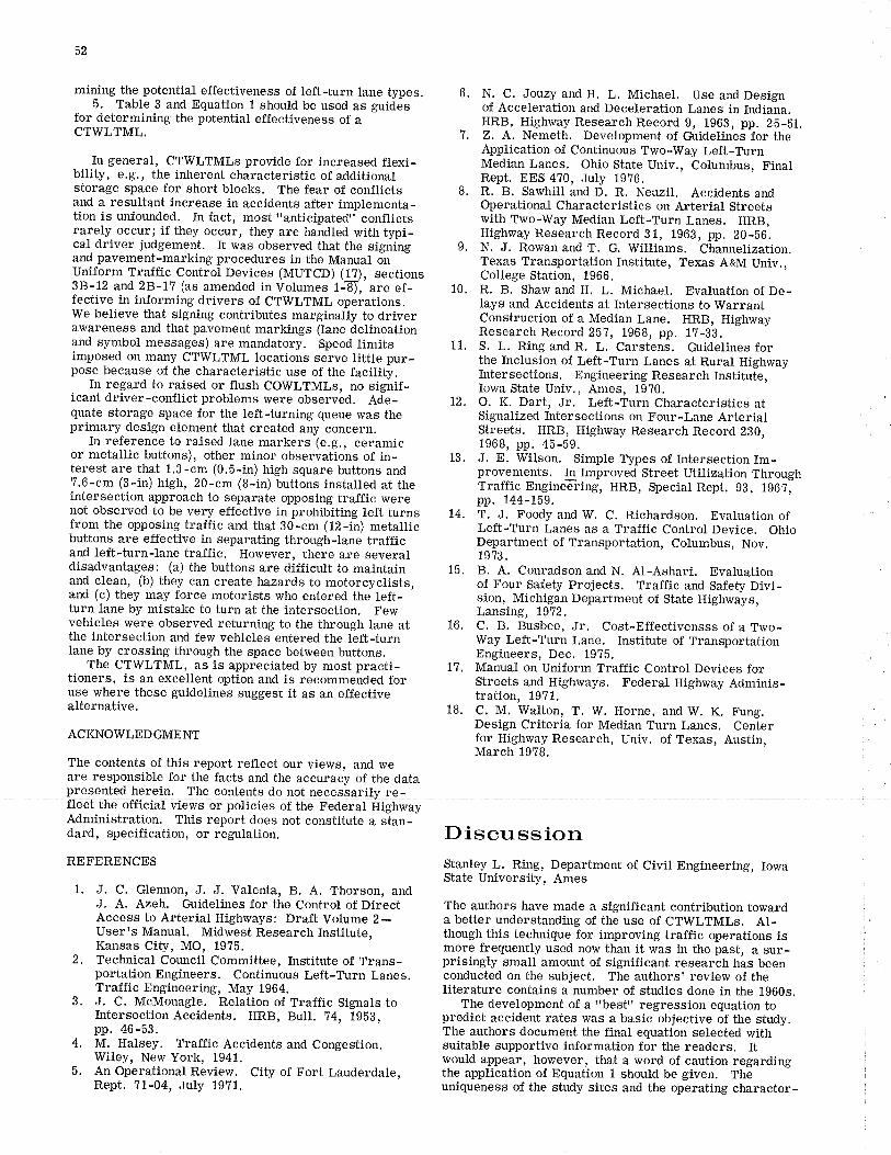
52
mining the potential effectiveness of left-turn lane types.5. Table 3 and Equation 1 should be used as guides
for determining the potential effectiveness of aCTWLTML.
In general, CTWLTMLs provide for increased flexi-bility, e.9., the inherent characteristic of additionalstorage space for short blocks. The fear of conflictsand a resultant increase in accidents after implementa-tion is unfounded, In fact, most t'anticipated" conflictsrarely occur; if they occur, they are handled with typi-cal driver judgement, It was observed that the signiìgand pavement-marking procedures in the Manual onUniform Traffic Control Devices (MUTCD) (1?), sections38-12 and 2B-17 (as amended in Volumes 1Æ), are ef-fective in informing drivers of CTWLTML operations.We believe that signing contributes marginally to driverawareness and that pavement markings (lane delineationand symbol messages) are mandatory. Speed limitsimposed on many CTWLTML locations serve litfle pur-pose because of the characteristic use of the facility.
In regard to raised or flush COWLTMLs, no signif-icant driver-conflict problems were observed. Ade-quate storage space for the left-turning queue was theprimary design element that created any concern.
In reference to raised lane markers (e.g., ceramicor metallic buttons), other minor observations of in-terest are that 1.3-cm (0.5-in) high square buttons and?.6-cm (3-in) high, 20-cm (B-in) buttons installed at theintersection approach to separate opposing traJfic werenot observed to be very effective in prohibiting left turnsfrom the opposing traffic and that S0-cm (12-in) metallicbuttons are effective in separating through-Iane traffi.cand left-turn-lane traffic, However, there are severaldisadvantages: (a) the buttons are difficult to maintainand clean, (b) they can create hazards to motorcyclists,and (c) they may force motorists who entered the left- '
turn lane by mistake to turn at the intersection. Fewvehicles were observed returning to the through lane atthe intersection and few vehicles entered the left-turnlane by crossing through the space between buttons.
The CTWLTML, as is appreciated by most practi-tioners, is an excellent option and is recommended foruse where these guidelines suggest it as an effectivealternative.
ACKNOWLEDGMENT
The contents of this report reflect our views, and weare responsible for the facts and the accuracy of the datapresented herein. The contents do not necessarily re-
Administration. This report does not constitute a stan-dard, specification, or règuhtion. DiSCtf SSiOn
Stanley L. Ring, Department of Civil Engineering, IowaState University, Ames
The authors have made a significant contribution towarda better understanding of the use of CTWLTMLs. AI-though this technique for improving traffic operations ismore frequently used now than it was in the past, a sur-prisingly small amount of significant research has beenconducted on the subject. The authors' review of theliterature contains a number of studies done in the 1g60s.
The development of a "besttt regression equation topredict accident rates was a basic objective of the study.The authors document the final equation selected withsuitable supportive information for the readers. Itwould appear, however, that a word of caution regardingthe application of Equation 1 should be given. Theuniqueness of the study sites and the operating character-
6. N. C. Jouzy and H. L. Michael. Use and Designof Acceleration and Deceleration Lanes in Indiana,HRB, Highway Research Record 9, 1963, pp, 25-51,
L Z. A. Nemeth. Development of G¡idelines for theApplication of Continuous Two-Way Left-TurnMedian Lanes. Ohio State Univ,, Columbus, FinalRept. EES 4?0, July 19?6,
L R, B. Sawhill and D. R. Neuzil. Accidents andOperational Characteristics on Arterial Streetswith Two-Way Median Left-Turn Lanes. HRB,Highway Research Record 31, 1968, pp. 20-b6.
I. N. J. Rowan and T. G. Wiltiams. Channelization.Texas Transportation Institute, Texas A&M Univ.,College Station, 1966.
10. R. B. Shaw and H. L. Michael. Evaluation of De-lays and Accidents at Intersections to WarrantConstruction of a Median Lane. HRB, HighwayResearch Record 257, 1968, pp. 17-33.
11. S. L. Ring and R. L. Carstens. G¡idelines forthe Inclusion of Left-Turn Lanes at Rural HighwayIntersections. Engineering Research Institute,Iowa State Univ,, Ames, 1970,
12. O. K. Dart, Jr, Left-Turn Characteristics atSignalized Intersections on Four-Lane ArterialStreets. HRB, Highway Research Record 280,1968, pp. 45-59.
13. J. E. Wilson. Simple Types of Intersection Im-provements. In Improved Street Utilization ThroughTraffic Engineiõring, HRB, Special Rept. 93, 196?;pp.144-159.
14. T. J. Foody and W. C. Richardson. Evaluation ofLeft-Turn Lanes as a Traffic Control Device. OhioDepartment of Transportation, Columbus, Nov,1973.
15. B. A. Conradson and N. Al-Ashari. Evaluationof Four Safety Projects. Traffic and Safety Divi-sion, Michigan Department of State Highways,Lansing, l9?2.
16. C. B. Busbee, Jr. Cost-Effectivensss of a Two-Way Left-Turn Lane. Institute of TransportationEngineers, Dec. 1975.
I7. Manual on Uniform Traffic Control Devices forStreets and Highways. Federal Highway Adminis-tration, l9?1.
18. C. M. Walton, T. W. Horne, and W. K. Fung.Design Criteria for Median Turn Lanes. Centerfor Highway Research, Univ, of Texas, Austin,March 1978.
REFERENCES
1. J. C, Glennon, J. J. Valenta, B. A, Thorson, andJ. A. Azeh. Gridelines for the Control of DirectAccess to Arterial Highways: Draft Volume 2-User's Manual. Midwest Research Institute,Kansas City, MO, 1975.
2. Technical Council Committee, Institute of Trans-portation Engineers. Continuous Left-Turn Lanes.Traffic Engineering, May 1964.
3. J. C. McMonagle, Relation of Traffic Signals toIntersection Accidents. HRB, Bull. 74, Lgïl,pp. 46-53.
4. M. Halsey. Traffic Accidents and Congestion.Wiley, New York, 1941.
5. An Operational Review. City of Fort Lauderdale,Rept, 71-04, July 19?1.
53
istics of the traffic fLow are related to the specific model citíes, this ingenious traffic engineering device is notpresented. In view of this applicable environmental con- being used to its full potential. In fact, it is not beingstraint, the reader should be cautioned in making appli-cations to other environments,
Also, it should be noted that a relatively large nega-tive intercept constraint exists in Equation 1. Again, aword of caution regarding the extension of the predictingrange beyond the data would be in order.
The operational study phase prcivided some usefuI re-sults. I was, however, somewhat concerned with theprocedure for measuring vehicle entrance and maneu-vering distance and lateral placement. ObservatÍonsfrom the side of the road "as far as possible from theroadway (in order to minimize influence on the driver)"would appear to introduce considerable judgment deci-sions and estimating because of visual shorteomings andparallax. A number of photographic or video studiesfrom elevated positions have been made in similar situa-tions and have yielded more reliability.
It has been reported that, in certain locations, ve-hicles entering the roadway from an entrance tend to
used at all in many cities, although the date of the firstinstallation goes back to at least 1950, when it was in-troduced in Michigan, There are various misconceptionsunderlying the resistance, and every bit of evidence re-garding the safety a¡d effectiveness of CTWLTMLSshould be shared with the traffic engineering community.
Every traffic engineer recognizes that urban arterialsusually perform two conflicting functions, namely theprovision of access to abutting land uses and the provi-sion of flow for through tra,ffic. By permittÍng parkingin the curb lane, for example, access is being favored,while the removal of curb parking increases the levelof service for the tra"ffic flow. CTWLTMLS can do both:They improve access to driveways and reduce delay tothrough traffic.
The main purpose of my comments is to support someof the findings of this paper. The basis for my commentsis mostly the information gathered in two different sur-veys of traffic engineers around the country: an earlier
use the CTWLTML for storage or for merging with adja- one in connection with sponsored research (7) and a re-cent through traffic at a moré convenient anglä. i; ;;" cent one in connection with the work of a coñmittee Icases, trucks especially benefit from these facilities.It would have been helpful if this aspect were observedand reported for the reader's total knowledge of benefits.
Other questions arose in regard to increased potential subject paper.for U-turns, signal progression as an independent vari-
chair for the Institute of Transportation Engineers (thissurvey resulted in 106 responses from 29 states).
My comments will be directed at three areas of the
1. Among the findings of the accident analysis Ís theinformation that "unsafe speed,r' "failing to yield theright-of-way," and "following too closely" are the majorcontributing factors in 70 percent of the accidents atCTWLTML sites. These factors are among the con-tributing factors commonly listed on standard accidentreporting forms and, in general, are not very usefulfor the purposes of cause-and-effect accident studies.The more important conclusion is that "CTWLTML siteshad only small percentages of midblock accidents in-volving vehicles slowing or stopping to make left turns.r'
I would like to add that, among the traffic engineerswho responded to the above-mentioned surveys, only 11
percent indicated that accident problems were experi-enced at CTWLTMLs. Furthermore, all but one of therespondents who reported accident problems also indi-cated that some problems existed with improper use ofthe median lane. In contrast, only 50 percent of the total
able, and changes in total vehicle delay, Answers maybe available in the detailed project report, or they mayhave been beyond the scope of this study. These ques-tions may be related to the limitations of the manualobservation technique.
The authors are to be commended overall for an ex-cellent study.
John C, Glennon, Overland Park, Kansas
I would like to commend the authors on their paper. Itoffers a significant contribution to our knowledge aboutIeft-turn median treatments. I have no other direct
flow and commercial-development conditions, Thestudies I recommend, therefore, would be aimed atdelineating the traffic operational benefits of two-wayIeft-turn medians under various conditions,
comments about the paper, but I would like to recom- the meclian lane. rn contrast, only Ðu pe.rcen[ or f,ne torar
mend further operational ét tdies. My observation is that survey population reported problems with improper use'several jurisdictions around the couniry are sti[ reluc- In other words, few CTWLTMLs have accident problemstant to try the two-way left-turn median. Although some and those that do also have problems with improper use' :
jurisdictions may be a-fraid of increased accidents, more As one of the respondents to the survey explained, I'mo-
âre probabty relüctant because of the lack of convíncing torists sometimes stop in the median lane at an angle,ttenceorrsignificænfbenefits. c¡ith the rear oflhe ear prot+uding'into the throughJan€- +uence on s¡.B¡u.rruarrl oellerrLs.It seems clãar that two-way left-turn medians would This causes some rear-end accidents, which most often
offer substantial delay reductions where traffic volumes do not involve the left-turning vehicles themselves."are moderate to high in strip commercial areas. Yet Also, sideswipe accidents occur when some drivers4¡ç ¡l¡wç¡4Lç !U r¡rÉr¡ ¡rr Þur¡l/ vur¡u¡!çru¡4 4¡ç4È. rs! '-F- -----'-_---no studies have cleãrly shown the capacity improvement enter the CTWLTMLs too early and travel down the la¡evalue of two-way left-iurn medians under various traffic- only to be struck by another driver entering the
CTWLTML nearer to the left-turn point.Sometimes right-angle collisions occur between ve-
hicles entering the CTWLTML from the through lane andvehicles exíting from a driveway and making a left turninto or across the CTWLTML.
Generally, the responses indicate that the incidenceof other types of accidents (especially head-on collisions)was very rare.
Some other improper uses reported in the surveysZoLtan A. Nemeth, Department of Civil Engineering, include turning improperly from the through lanes, pass-Ohio State University,'Columbus ing slower vehicles for many blocks in the CTWLTML
before turning left, truckers stopping for loading or un-Let me begin by congratulating the authors of this valu- loading, bicyclists using it as a bike way' Improperable contribution to the very limited literature on uses that are due to unfamiliarity will' of course, di-CTWLTMLS. With the excêption of a few states and minish in time. At the beginning, however' education
54
of the public is important, and the cooperation of theenforcement agencies is needed, (In an extreme caseof noncooperation, one respondent reported that, in anearly use, the police considered CTWLTMLs to be me-dian divider islands and ticketed left-turning vehicles.)
I would like to add that CTWLTMLs can, in case ofemergency, provide a path for emergency vehicles, adetour lane during blocking of through lanes by construc-tion or vehicle breakdown, or even a place for storingsnow removed from the through lanes.
2. The accident prediction equation (Equation 1)includes only four independent variables, and they arereadily available. This should make it easy for othersto test the equation and compare results, It was sur-prising at first to find that operating speeds were notincluded among the independent variables. A closerlook at the study-site characteristics revealed, however,that speed limits ranged mostly from 48 to 64 km/h (30-40 mph) lonly one site had a12-km/h (45-mph) speedlimitl, In this range, apparently, speed has no signifi-cant effect on accident statistics. It would have been in-teresting to see the effect of higher operating speed.Fifty-seven percent of the respondents to our surveysuggested that the speed limit should be less than 88km/h (55 mph) on arterials where CTWLTMLs are tobe introduced. On the other hand, there are severalexamples of CTWLTMLs working properly even at 105km/h (65 mph) (prior to imposition of the 88-km,/h speedlimit). One respondent stated that there is "no magicinvolved in the speed-limit sign. We have TWLTLs formiles on open rural unposted state highways,..," It isprobable, however, that, if the frequency of midblockleft turns justifies CTWLTMLs, then the lower speedIimit is also justified by the intensity of roadside devel-opment.
3. The paper states that the authors believe thatsigning contributes marginally to driver awareness but
vehicles. These comments indicate that many agencieshave a rational approach to the decision on overheadversus side-m'ounted signs.
MUTCD itself has gone through severâI changes re-garding the subject of signing CTWLTMLs. I am notat all sure that I am aware of all the relevant changes,but let me attempt to summarize briefly my understand-ing of the evolution of the relevant sections in MUTCD:(a) Section 2 B-11 stated that signs "shall" be used,while Section 3 B-12 stated that signs "should" be usedwith pavement markings (19?1); (b) Change M-24 (9/21/?4) eliminated the contradiction by changing'rshould'r to?tshallrt in Section 3 B-12; (c) Change Sn-156 (6/25/16\stated that "The R3-9 or R3-9a sÍgn shall be mountedoverhead and over the two-way left-turn lane when thereare more than three lanes"; and (d) Change: Reconsid-eration of Ruling Sn-156 (9/LS/11)t 'rThe post-mountedR3-9b sign may be used as an alternate to or a supple-ment to the overhead-mounted R3-9a sign,"
In conclusion, let me state again that two-way left- .turn lanes provide a good solution to the problem createdby midblock left turns. Starting-up problems can be ex-pected when they are first introduced in an area. How-ever, they provide such an obviously needed service thatdrivers will soon get used to them and the level of im-proper use will drop to a minimum, as with other formsof traffic control.
Authors' ClostlreWe wish to express our appreciation to those who sub-mitted discussions. These discussions emphasize that,
that pavement markings, including arrows, are essen- in general, the vast majority of current e¡perience withtial. The MUTCD (1?) requires both signs and pavement CTWLTMLS indicates that accident problems are not amarkings. primary deterrent to the use of these facilities. Ex-
Our surveys found that g6 percent of the respondents cessive accident rates seem to be related to impropercomplied with the MUTCD for pavement markings and use of CTWLTMLS; the comþination of appropriate con-76 percent did for signing. At least one respondent even trol devices and driver e4perience should have a positiveexpressed concern that ihe e>.penses involved in the re- effect on this situation,quired signing may keep some agencies from installing MUTCD (17) does require that signs, as well as pave-CTWLTMLS. Some agencies reported that they use signs ment markings, be used along CTWLTMLS, The re-to comply with MUTCD, but they do not really think that consideration (9/LS/11) of Change Sn-156 allows a choicethey are necessary. Some 50 percent of the reporting between post- and overhead-mounted signs. Opinionsagencies use overhead signs as well as ground-mounted expressed by the vast majority of those contacted duringsigns. Some interesting comments were received from this reserach indicate that driver response to pavementthem regarding their policy on overhead signs: They use markings is clearly more positive than that for post-
erhea* signs whersobliteratiorrof pavenre¡t markings-Írounteù oroverhead:rnounted sig¡s; ás-noted-irrtheby snow can be expected, where curb parking or roadside discussions, areas where markings are often obliterateddevelopment can detract from ground-mounted signs, by snow have definite need for effective signage.where frequent improper use has been observed during In summary, the CTWLTML is an effective and ef-use of pavement markings and ground-mounted signs, ficient treatment for midblock turn problems, Its con-and on major multilane streets that have frequent sig- trolled use is recommended for a substantial varietynalized intersections. They reported that overhead signs of conditions.are spaced at quarter to half points between major in-tersections, no less than 305 m (1000 ft) apart at otherIocations, and no less than 46 m (150 ft) away from major pubtication of th¡s paper sponsored by Committee on Operationalintersections to ensure adequate visibility for turning Effects of Geometrics.
55
Abridement
Benefit-Cost Analysis of AdvanceTreatment for No-Passing ZonesDonald L. \iloods and Graeme D. Weaver, Terca.s Transportation
Institute, Te)Ê.s A&M University, College Station
It was the objective of a recent Federal Highway Ad- fession are constantly forced to apportion alreadyministration (rnw¡) research project Q) to devetop scarce funds to those areas in wtriõtr they believe theimproved criteria and guidelines for establishing pass- greatest return will be achieved.ing and no-passing zones, regulatory traffic control The concept of advance notification is a philosophydevices, and traffic regulations, enforcement methods, generally regarded among traffic engineers as beingand legal requirements that can be uniformly applied highly desirable in eliciting proper driver responsethroughout the nation for the safety and benefit of aII and, therefore, as contributing noticeably to highwaydrivers. Alternative methods of establishing and desig- safety, The need for advance warning of a no-passingnating passing and no-passing zones were developed to zone is evidenced by the rapidly spreading adoption ofenhance current practice to supply the safety needs. the NO PASSING ZONE pennant sign, the primaryThe suggested system was selected because it exhibited approved traffic control device for this purpose. Inthe greatest feasibility on the basis of driver under- many cases, the administrative decision to adopt thestanding, continuity of accepted type of demarcation concept of advance warning for the no-passing zone(longitudinal line adjacent to roadway centerline), appears not to have been made on the basis oi a de-satisfaction of the driverrs visual information needs, tailed benefit-cost analysis but rather as the result ofand practicality of installation and maintenance with the conviction that driver conditioning to potentialexisting mechanized striping equipment. It consisted hazard is in itself beneficial and the cost of implement-of a dotted yellow line adjacent to the roadway centerline ing such a system will be offset by improved operationsthroughout the do',vnstream end of the passing zone in and safety and reduced potential for litigation, althoughconjunction with the standard NO PASSING ZONE pen- these elements may not have been quantified precisely.nant sign at the beginning of the no-passing zone's solid The concepts developed in the research regardingyellow barrier stripe. criteria, application, and design of the traffic control
The details of criteria development, driver under- devices by which no-passing zones should be establishedstanding studies, and research methodology are included and designated (1) were critically reviewed by 36 trafficin the final report Q) ana are not discussed here, but engineeri in various parts of the country and by a groupthe salient research results are summarized belo',v: of members of the National Advisory Committee on
Uniform Traffic Control Devices and FHWA in a two-1. To avoid ambiguity in definitive terminology re- day workshop. In general, the concepts remained un-
lating to the passing maneuver, the distance elements in- challenged; the primary concern erpressed was that
is defined as the sight distance at which a passing driver provide a framework for basing a decision to evaluate,at the critical position (passing and passed vehicles in actual operation, a concept [hat theoretically appearedabreast) must be able to perceive an opposing vehicle to sound and ieasonable. In response to this rather unani-permit safe completion of the maneuver. mous expression of opinion, ai economic analysis was '
.3, A concept of advance marking treatment pre- conducteã to predict the expected benefit-cost ratio ofceding a no-passing zone demarcation system with a application ofthe advance-warning no-passing-zone treat-
r NO PASSING ZONE pennant at the beginning of the solid ment proposed in the research effort. This abridged'yellow no-passing-zone line was suggested as a system paper presents the results of the economic analysis. i
oFtraf f I sgonfroffi evlsssthaf wo uld p ro vide t he neede ddriver information to designate that the passing zone will General Approachsoon end and that a no-passÍng zone will be reached.
4. Establishment of a no-passing-zone system should The intent during the economic analysis was to be con-be predicated on minimum passing sight distance for a servative, so that the resulting benefit-cost ratio wouldspecified operating speed, The advance marking treat- represent a very conservative estimate of the relativement begins at the point at which sight distance first value of the system. In all probability, the benefitsbecomes less than the specified minimum passing sight would be substantially greater. To ensure conserva-distance and continues for a distance equal to the pass- tism, several assumptions were made: (a) relativelycompletion distance for the specified operating speed; short sign life was assumed, (b) only those drivers whothe no-passing zone begins at the downstream end of the "clip" the no-passing zone (complete the pass beyondadvance marking treatment and continues until the the start of the solid yellow line) were asiumed to bene-minimum passing sight distance again becomes available. fit from the advance treatment, and (c) an interest rate
on the high side was assumed.
volved in the maneuver r,vere defined as illustrated inFigure 1.
2, Minimum passing sight distance (2/3dz + dg + d+)
PURPOSE OF THE ECONOMICANALYSIS
Traditionally, one of the primary considerations inevaluating a proposed change in concept or practiceinvolves the question, What benefits can be expectedfrom the change ? Administrators in the highway pro-
there was a definite need to evaluate the benefits thatcould reasonably be expected from implementation of theproposed treatments for no-passing zones, This would
The approach adopted to compare expected benefitswith expected costs on a nationwide basis included esti-mating the (a) costs of proposed no-passing-zone advancetreatment nationwide, (b) number of no-passing zonesnationwide, (c) number of passing maneuvers executedannually on two-lane highways nationwide, (d) numberof passing maneuvers that involve "clipping", (e)
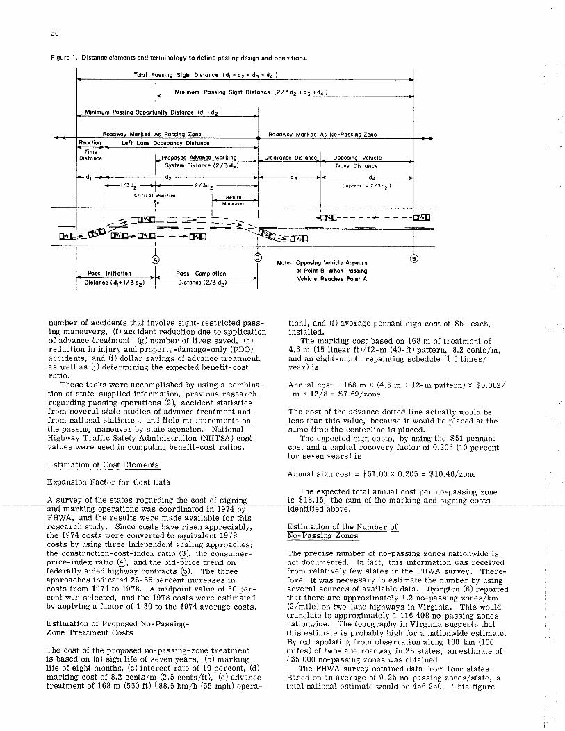
Totol Dlstonca (dr + dr + d¡ + d¿ )
I, r f*¡nimum Possing Slght Distonce (2/f,dz + dt +d4 ) rI
Minimum tuss¡no ODoorlunilv Dislorce (dr + da ) I
-r
Roodwoy Morhed As Possinq Zone 1 Roo¿*o, Morked As No-Possinq Zone
ñæclirrn ¡ . l:'lf Lona OccuÞoncy Dlslonce
,Cleoronce Disloæe I Oggosinq V€hicleTime '
0islonc€
-t
Proposed Advonce MorkinSyslem Dislonco (2/ 3 dz) Trovel Dislonc€
'r3d- >l 2t!¿- +
Cñlrcol Po¡il¡d I R¡turnfc f-nñ;;-
I Apyox = 2/3d21
56
Figure 1. Distance elements and terminology to def¡ne passing design and operations.
+
Poss ln¡tlotlon Poss Complellon
Dastonc. (dt+ l/3da) Dlsionce (2Æ dr)
tionl, and (f) average pennant sign cost of $51 each,installed.
The marking cost based on 168 m of treatment of4.6 m (15 linear ft)h2-m (40-ft) pattern, 8.2 cents/m,and an eight-month repainting schedule (1.5 times/vear) is
Annual cost = 168 ¡1 x (4.6 m + 12-m pattern) x $0.0S2/mxtZ/B=97.65/zone
The cost of the advance dotted line actually would beless than this value, because it would be placed at thesame time the centerline is placed,
The e:ipected sign costs, by using the $51 pennantcost and a capital recovery factor of 0.205 (10 percentfor seven years) is
Annual sign cost = $51.00 x 0.205 = $10.46/zoneExpansion Factor for Cost Data
The ex¡pected total annual cost per no-passing zoneA survey of the states regarding the cost of signing is $18.15, the sum of the marking and signing costs
FHWA, and the results were made available for thisresearch study. Since costs have risen appreciably,the 19?4 costs were converted to equivalent 19?8costs by using three independent scaling approaches:the construction-cost-index ratio (3), ttre consumer-price-index ratio (l), and the bid-price trend onfederally aided highway contracts (5). The threeapproaches indicated 25-35 percenfincreases incosts from 19?4 to 1978. A midpoint value of 30 per-cent was selected, and the 1978 costs were estimatedby applying a factor of 1.30 to the 1974 average costs.
Estimation of Proposed No- Passing-Zone Treatment Costs
The cost of the proposed no-passing-zone treatmentis based on (a) sign life of seven years, (b) markingIife of eight months, (c) interest rate of 10 percent, (d)marking cost of 8.2 cents/m (2.5 cents^t), (e) advancetreatment of 168 m (550 ft) [eA.¡ tm/h (55 mph) opera-
Note, Oppcing Veh¡cle Appcoreot Po¡nt B lfhcn PossingV€hicle RôodÉs Polnl A
number of aecidents that involve sight-restricted pass-ing maneuvers, (f) accident reduction due to applicationof advance treatment, (g) number of lives saved, (h)reduction in injury and property-damage-only (PDO)accidents, an¿ (i) dollar savings of advanee treatment,as rvell as (j) determining the expected benefit-costratio,
These tasks were accomplished by using a combina-tion of state-supplied information, previous researchregarding passing operations (?), accident statisticsfrom several state studies of advance treatment andfrom national statistics, and field measurements onthe passing maneuver by state agencies. NationalHighway Traffic Safety Administration (NHTSA) costvalues tffere used in computing benefit-cost ratios,
Estimation of Cost Elements
Estimation of the Number ofNo-Passing Zones
The precise number of no-passing zones nationwide isnot documented, In fact, this information was receivedfrom relatively few states in the FHWA survey. There-fore, it 'r¡as necessary to estimate the number by usingseveral sources of available data. Byington (6) reportedthat there are approximately 1.2 no-passing zõnes/km(2/mile) on two-lane highways in Virginia. This wouldtranslate to approximately 1 116 408 no-passing zonesnationwide. The topography in Virginia suggests thatthis estimate is probably high for a nationwide estimate.By extrapolating from observation along 160 km (100miles) of two-lane roâdway in 28 states, an estimate of835 000 no-passing zones was obtained.
The FHWA survey obtained data from four states.Based on an average of 9125 no-passing zones/state, atotal national estimate would be 456 250. This figure
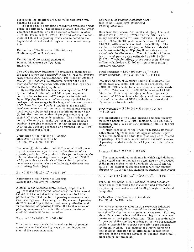
represents the smallest probable value that could rea-sonably be expected.
The three basic esimating procedures produced a widerange of estimates. The average is about 800 000, whichcompares favorably with the estimate obtained by sam-pling 160 km in several states, For this reason, the esti-mate of 835 000 no-passing zones was selected as theexpected value and used throughout the economic analy-sis.
Estimation of the Benefits of the Advance
Estimation of the Annual Number ofPassing Maneuvers on Two-LaneHighways
The 1974 Highway Statistics [) presents a summary ofthe length of two-lane roadway in each of several averagedaily traffic (ADT)classifications. The Highway CapacityManual (8) presents a relationship between the peakloadings and the frequency with which the loadings occuron the two-lane highway system.
By multiplying the average percentage of the ADTby the midpoint value of the ADT ranges, ex¡lectedhourly volumes for each ADT range can be obtained,By multiplying the number of hours represented by thepeak-period percentage by the length of roadway in eachADT classification, hourly kilometers at each ADTlevel can be generated. By using relationships betweentotal hourly volume and passes per kilometer per hour(9,10), the average number of passing maneuvers foreãc-h ADT group can be determined. The product of thehourly kilometers at each ADT level and the averagenumber of passing maneuvers for that group summedover all ADT groups produces an estimated 7461.2 x tO6passing maneuvers/year.
Estimation of the Number of PassingManeuvers Performed with NoOn-Coming Vehicle in Sight
Normann (11) determined that 59.? percent of all pass-ing maneuvers were performed in the absence of anopposing vehicle, The product of this percentage and thetotal-number of passing maneuvers performed (7451,2x 10o) provides an estimate of the number of passingmaneuvers executed when available sight distance wasthe limiting factor (P,^).
Psn = 0.597 x 7451.2x 106 = 4448x 106
51
Estimation of Passing Accidents ThatInvolve an lllegal Sight- RestrictedPassing Maneuver
Data from the Federal Aid Fatal and Injury AccidentRate Study in 19?4 (13) reveal that the fatality andinjury accident rates for rural federal aid highwayswere 1.99 and 3?/100 million vehicle-km (3.2 and59.5h00 million vehicle miles), respectively. Thenumber of fatalities and injury accidents eliminatedcan be estimated by multiplying these rates and theannual vehicle kilometers. The total vehicle kilome-ter of travel per day was estimated as 849.1 x 10⁶(SZl .l x 106 vehicle miles), which represents 309 800million vehicle-km (192 600 million vehicle miles)annually; therefore,
Fatal accidents = 1.99 x 309 800 x 10-'z = 6160Injury accidents = 3? x3Og 800x 10-2 = 114 600
The 1974 edition of Accident Facts (14) indicates that19 300 fatal accidents, 230 000 injury accidents, and2 240 000 PDO accidents occurred on rural state roadsin 19?3. This resulted in 420 000 injuries and 23 300fatalities. E>çanding the injury accÍdent figures bythe ratio of PDO accidents to injury accidents, an esti-mate of the number of PDO accidents on federal aidhighways can be obtained:
PDO accidents = (2 240 000 + 230 000) x 114 600= 1 116 000
The distribution of two-lane-highway accident severitytherefore becomes 6160 fatal accidents, 114 600 injurvaccidents, and 1 116 000 PDO accidents(total=1 236?60accidents).
A study conducted by the Franklin Institute ResearchLaboratories (9) concluded that approximately 10 per-cent of the accidents on two-Iane roadways were relatedto passing. Therefore, an estimate of the total numberof passing-related accidents is 10 percent of the valuesabove:
4"o.",'o = 0.10 x 1 236 ?60 = 123 676
The passing-related accidents in which sight distanceis the visual restriction can be estimated by the productof the total passing-related accidents (Aro..,ro) and theratio of the number of passing manuevers that involveclipping (P"r,r) to ttre tõtal number of passing maneuvers:
Estimation of the Number of PassingManeuvers That Involve ClÍpping
A study by the Michigan State Highway Department(12) revealed that clipping (completing the pass beyondthe start of the solid yellow line) occurred in 14-1?percent of the total number of passing maneuvers on atwo-Iane highway. Assuming that 15 percent of passingdrivers would clip in the normal passing situation andin the absence of opposing traffic, the total number ofpassing maneuvers for which the advance treatmentcould be beneficial is estimated as
Pcup = 0.15 x4448x 106 = 66? x 106
This number represents the annual number of passingmaneuvers on two-lane highways that end beyond thestart of the no-passing zone,
Acurp = 123 676 x 667 x 451x1 11 071
Thus, an estimated 11 071 passing-related accidentsoccur annually in which the maneuver was initiated inthe passing zone and involved an illegal sight-restrictedcompletion.
Estimation of the Number of AccidentsThat Wou1d Be Eliminated
The human-factors studies in this research indicatedthat approximately 14 percent of the subject driversoccasionally clip during the passing maneuver. Further,about 69 percent understood the meaning of the advancetreatment without prior education. Thus, approximately51 percent of the drivers (product of the two percentages)could be expected to respond correctly to the advancetreatment system. The number of clipping accidentsthat could be e¡gected to be eliminated through exten-sive use of the proposed advance no-passing-zone treât-ment can be estimated as
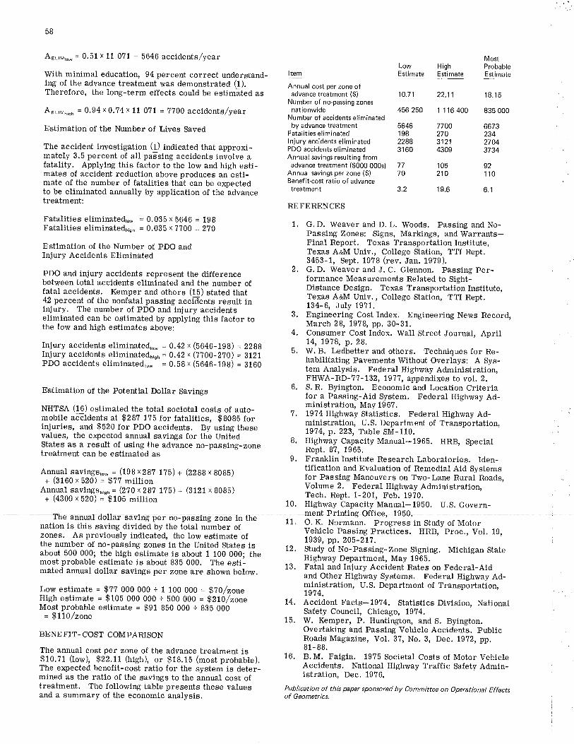
58
Ar.,",o* = 0.51 x 11 0?1 = 5646 accidents/year
With minimal education, 94 percent correct understand-ing of the advance treatment was demonstrated (1).Therefore, the long-term effects could be estimãted as
A.r'rn,nn = 0.94 x 0'74 x 11 0?1 = 7?00 accidents/year
Estimation of the Number of Lives Saved
The accident investigation (1) indicated that approxi-mately 3.5 percent of all paFsing accidents involve afatality. Applying this factor to the low and high esti-mates of accident reduction above ptoduces an esti-mate of the number of fatalities that can be expectedto be eliminated annually by application of the advancetreatment:
Fatalities eliminated,* = 0.035 x 5646 = 198Fatalities eliminated¡¡n¡ = 0.035 x7700 = 270
Estimation of the Number of PDO andInj ury Accidents Eliminated
PDO and injury accidents represent the differencebetween total accidents eliminated and the number offatal accidents. Kemper and others (15) stated that42 percent of the nonfatal passing accidents result ininjury. The number of PDO and injury accidentseliminated can be estimated by applying this factor tothe low and high estimates above:
Injury accidents eliminatedr* = 0.42 x (b646-19B) = 22BBInjury accidents eliminatedn,nn = 0.42 r (7700-2?0) = 3121PDO accidents eliminated,o* = 0.bB x (b646-198) = 3160
Estimation of the Potential Dollar Savings
NHTSA (16) estimated the total societal costs of auto-mobile accidents at $28? 1?5 for fatalities, g808b forinjuries, and $520 for PDO accidents. By using thesevalues, the e4gected annual savings for the UnitedStates as a result of using the advance no-passing-zonetreatment can be estimated as
Annual savingsrow = (198 xZg? 175) + (2ZBB x B0Bb)+ (3160 x 520) = $?? million
Annual savingsn¡n¡ = (270 x 281 Lj5) + (3121 x B0Bb)+ (4309 r 520) = $105 million
nation is this saving divided by the total number ofzones. As previously indieated, the low estimate ofthe number of no-passing zones in the United States isabout 500 000; the high estimate is about 1 100 000; themost probable estimate is about 835 000. The esti-mated annual dollar savings per zone are shown below.
Low estimate = $7? 000 000 + 1 100 000 = g?O/zoneHigh estimate = $105 000 000 + 5OO 000 = g?tl/zoneMost probable estimate = $91 850 000 + 83b 000
= 9110/zone
BENEFIT. COST COMPARISON
The annual cost per zone of the advance treatment is$10.?1 (low), $22.11 (high), or 918.1b (most probabte).The expected benefit-cost ratio for the system is deter-mined as the ratio of the savings to the annual cost oftreatment. The following table presents these valuesand a summary of the economic analysis.
Item
Annual cost per zone ofadvance treatment ($)
Number of no-passing zonesnationwide
Number of accidents eliminatedby advance treatment
Fatalities eliminatedI njury accidents eliminatedPDO accidents eliminatedAnnual savings resulting from
advance treatment ($000 000s)Annual savings per zone ($)Benefit-cost ratio of advancetreatment
REFERENCES
LowEstimate
MostHigh ProbableEstimate Estimate
10.7 1 22.11 18.1 5
456250 1 116400 835000
1. G. D. Weaver and D. L. Woods. Passing and No-Passing Zones: Signs, Markings, and Warrants-Final Report. Texas Transportation Institute,Texas AaM Univ., College Station, TTT Rept.3453-1, Sept. 1978 (rev. Jan. 1979).
2, G. D. Tffeaver and J. C, Glennon, Passing Per-formance Measurements Related to Sight-Distance Design. Texas Transportation Institute,Texas AaM Univ., College Station, TTI Rept.134-6, July 19?1.
3. Engineering Cost Index. Engineering News Record,March 28, t978, pp. 30-31.
4. Consumer Cost Index. Wall Street Journal, April14, 1978, p, 28.
5. W. B. Ledbetter and others. Techniques for Re-habilitating Pavements'vVithout Overlays: A Sys-tem Analysis. Federal Highway Administration,FH\IVA-RD-71-132, 1971, appendixes to vol. 2.
6. S. R. Byington. Economic and Location Criteriafor a Passing-Aid System. Federal Highway Ad-ministration, May 1967.
7. 19?4 Highway Statistics. Federal Highway Ad-ministration, U,S, Department of Transportation,1974, p.223, Table SM-110.
8. Highway Capacity Manual-1965. HRB, SpecialRept. 87, 1965.
9. Franklin Institute Research Laboratories. Iden-tification and Evaluation of Remedial Aid Systemsfor Passing Maneuvers on Two-Lane Rural Roads,Volume 2. Federal Highway Administration,Tech. Rept. 1-201, Feb. 19?0.
10. Highway Capacity Manual-1950. U.S. Govern-
vehi cle pas sing p ractic"JJ. "irîäl' pîö'iår. r s,
1939, pp. 205-2L1.Study of No-Passing-Zone Signing. Michigan StateHighway Department, May 1965.Fatal and Injury Accident Rates on Federal-Aidand Other Highway Systems. Federal Highway Ad-ministration, U,S. Department of Transportation,1914.Accident Facts-19?4. Statistics Division, NationalSafety Council, Chicago, 19?4.'vV. Kemper, P. Huntington, and S. Byington.Overtaking and Passing Vehicle Accidents. PublicRoads Magazine, Vol. 37, No. 3, Dec. 19?2, pp.81- 88.B.M. Faigin. 1975 Societal Costs of Motor VehicleAccidents. National Híghway Traffic Safety Admin-istration, Dec. 1976.
Publication of this paper sponsored by Committee on Operational Effectsof GeometrÍcs.
5646 7700 6673198 270 2342288 3121 27043160 4309 3734
77 105 9270 210 1f0
3.2 19.6 6.1
Iãr saviñg per no-passing zone in the ., mentPrintirls=offieet a9Sno rlir¡irta¡t lrrr #ha jaror n,,*ha- ^r ,1, O. K. Normann. progress in Study of Motor
12.
13.
L4.
15.
16.
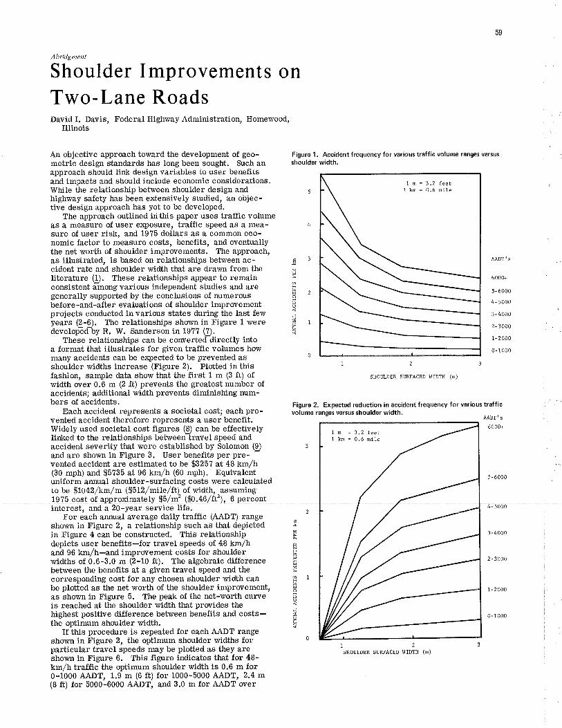
59
Abridgment
Shoulder Improvements onTwo-Lane RoadsDavid I. Davis, Federal Highway Administration, Homewood,
Illinois
An objective approach toward the development of geo-metrÍc design standards has long been sought. Such anapproach should link design variables to user benefitsand impacts and should include economic considerations.While the relationship between shoulder design andhighway safety has been extensively studied, an olojec-tive design approach has yet to be developed.
The approach outlined inthís paper uses traffic volumeas a measure of user exposure, traffic speed as a mea-sure of user risk, and 19?5 dollars as a common eco-nomic factor to measure costs, benefits, and eventuallythe net worth of shoulder improvements. The approach,as illustrated, is based on relationships between ac-cident rate and shoulder width that are drav¡n from theliterature (!). These relationships appear to remainconsistent among various independent studies and aregenerally supported by the conclusions of numerousbef ore -and -afte r evaluations of shoulde r improv e mentprojects conducted in various states during the þst fewyears @-p). The relationships shown in Figure 1 weredevelopGd by R. W. Sanderson in 1977 þ.
These relationships can be converted directly intoa format that illustrates for given traffic volumes howmany accidents can be e>rpected to be prevented asshoulder widths increase (Figure 2). Plotted in thisfashion, sample data show that the first 1 m (3 ft) ofwidth over 0.6 m (2 ft) prevents the greatest number ofaccidents; additional width prevents diminishing num-bers of accidents.
Each accident represents a sociefal cost; each pre-vented accident therefore represents a user benefit.Widely used societal cost figures ($ can be effectivelylinked to tlte relationships between travel speed andaccident severity that were established by Solomon (p)and are shown in Figure 3. User benefits per pre-vented accident are estimated to be $325? at 48 km/h(30 rnph) and $5735 at 96 km/h (60 mph). Equivalentuni.f orm annual shoulder -surfacing costs were calculated
Figure 1, Accident frequency for various traffic volume ranges versusshoulder width.
4
-3
H
âoO
JÉrz
AADT's
6000+
5- 6000
4- 5000
3-4ó00
2-3000
1- 2000
0- 1000
t23SHOTLDER SURFACED WIDTH (m)
Figure 2. Expected reduct¡on in accident frequency for various trafficvolume rançs versus shoulder width.
AAD',s
1m=3.2feet1 lm = 0.6 mile
lm =3.2feet1 km = 0.6 nile
to be $1042lkm/m \fi512/mile/ft) of width, assumingof anoroximate .46 6 percent
interest, and a 2O-year service life.For each arurual average daily trafïic (AADT) range
shown in Figure 2, a relationship such as that depictedin Figure 4 canbe constructed. This relationshipdepicts user benefits-for travel speeds of 48 km/hand 96 km/h-and imprwement costs for shoulderwidths of 0.6-3.0 m (2-10 ft). The algebraic differencebetween the benefits at a given travel speed and thecorresponding cost for any chosen shoulder width canbe plotted as the net worth of the shoulder improvement,as shown in Figure 5. The peak of the net-worth curveis reached at the shoulder width that provides thehighest positive diflerence between benefits and costs-the optimum shoulder width.
If this procedure is repeated for each AADT rangeshown in Figure 2, the optimum shoulder widths forparticular travel speeds may be plotted as they areshov¡n in Figure 6. This figure indicates that for 48-km/h traffic the optimum shoulder width is 0.6 m for0-1000 AADT, 1.9 m (6 ft) for 1000-5000 AAÐT, 2.4 m(8 ft) for 5000-6000 AADT, and 3.0 m for AADT over
êts
Ø1F
aoo¡Þzz
5-6000
0- 1000
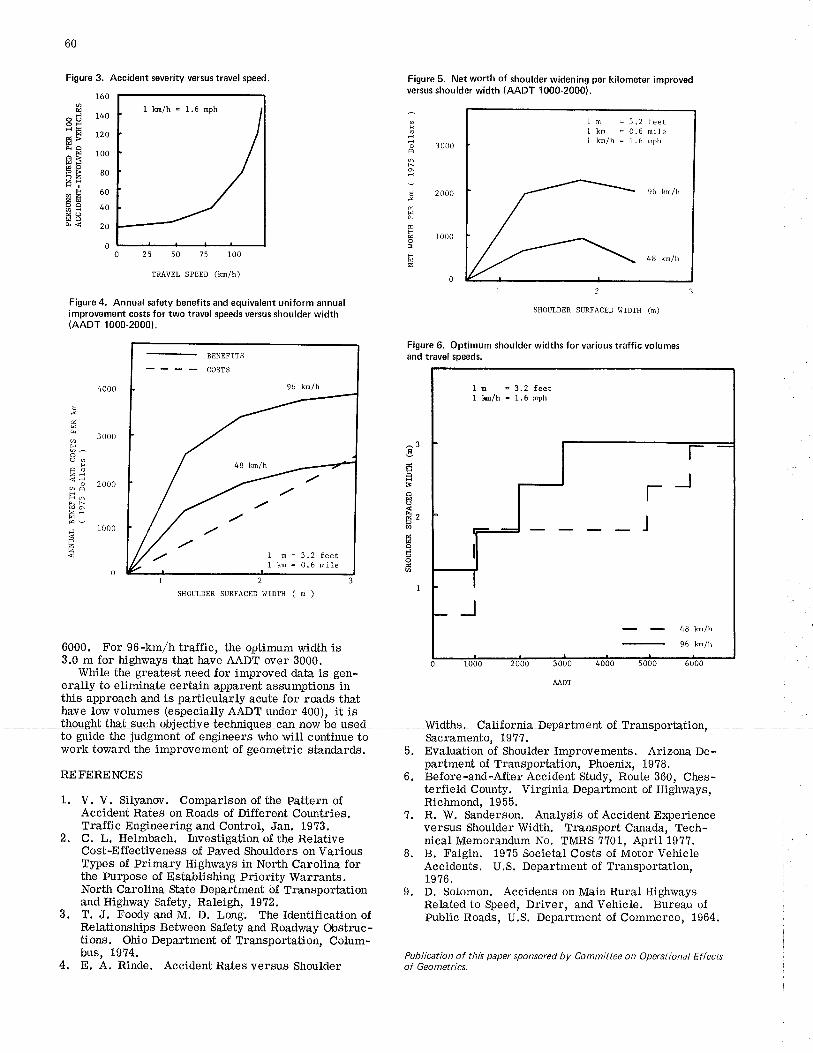
160
Hod 140OH
gH 120
Aâ^a 100HJÉoBÈ 80ZHHl
-E 60ZH3Ê 40&aÞoA< 20
o
60
Figure 3. Accident severity versus travel speed.
1 kn/h = 1.6 nph
25 50 75 100
TRAVEL SPEED (kn/h)
Figure 4. Annual safety benefits and equ¡valent uniform annualimprovement costs for two travel speeds versus shoulder width(AADT 1000.2000).
Figure 5. Net worth of shoulder widening per kilometer improvedversus shoulder width (AADT 1000-2000).
!
oa
noBts
3000
2000
1000
0
1m =3.2feet1 km = 0.6 mileI kn/h = 1,6 'O¡
48 km/h
.v
tso
zÅo
ts
Jsz
4000
3000
2000
1000
0
BENEFITS
- COSTS
48 km/h
,/ .// 1 m=3.2feer
1 kn = 0.6 nile
SHOULDER SURFACED WIDTH (m)
3000
AÀDT
Figure 6. Optimum shoulder widths for various traffic volumesand travel speeds.
1n =3.2feetI h/h = 1,6 0ph
r-Jr
I
I48 I'm/h
96 kn/h
^3E
FÊBaHo
É'ÊEôÉoE:ø
2
SHOULDER SURFACED WIDTH ( n )
6000. For 96-km/h trafTic, the optimum widttr is3.0 m for highways that have AADT over 3000.
While tìe greatest need for improved data is gen-eraUy to eliminate certain apparent assumptions inthis approach and is particularly acute for roads thathave low volumes (especially AADT under 400), it isthought that such obiectíve techniques can¡ow be used wirlt¡s. C¿liforni¿ìepartrnerrt of T'ansportation"to guide the judgment of engineers who ï/ill continue to Sacramento, 19??.work toward the improvement of geometric standards. 5. Evaluation of Shoulder Improvements. Arizona De-
REFEREN.ES 6. å?iffi"åliitri"J?'Jllaiåiiähånl3ö, "n""-terfield County. Virginia Department of Highways,
1. V. V. Silyanov. Comparison of the Pattern of Richmond, 195b.Accident Rates on Roads of Different Corurtries. 7. n. W. Sanderson. Analysis of Accident ExperienceTraffic Engineering and Control, Jan. 1973. versus Shoulder \ryifth. Transport Canada, Tech-2. C. L. Heimbach. Investigation of the Relative nical Memorandum No. TMRS ??01, April'19?7.Cost-Effectiveness of Paved Shoulders on Various g. B. Faigin. 19?b Societal Costs of Uotõr VehicleTypes of PrÍmary Highways in North Carolina for Accideñts. U.S. Department of Transportation,the Purpose of Establishing Priority \üarrants. 19?6.North Carolina Süate Department õf Transportation 9. D. Solomon. Accidents on Main Rural Highways
- and Highway Safety, Raleigh, 1972. Retated to Sþeed, Driver, and Vehicle. Bureau of3. T. J. Foody arld M. D. Long. The ldentification of public Roadè, U.S. Oepaitment of Commerce, 1964.Relationships Between Sa-fety and Roadway Obstruc-tions. Ohio Department of Transportation, Colum-
. bus, 1974. Publication of this paper sponsored by Committee on Operational Effects4. E. A. Rinde. Accident Rates versus Shoulder of Geometrics.
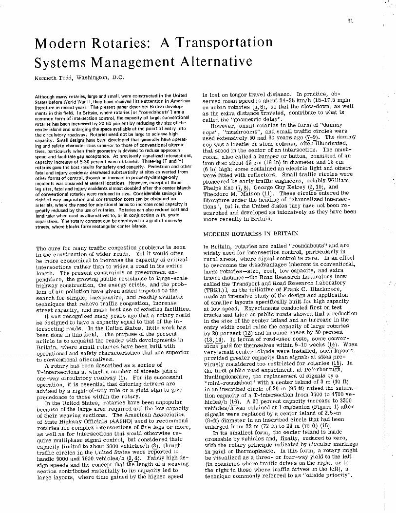
Modern Rotaries: A TransPortationSystems Management AlternativeKenneth Todd, Washington, D.C.
Although many rotaries, large and small, were constructed in the United
States before World War I l, they have received l¡ttle attention in American
literature ¡n recent years, The present paper describes British develop-
ments in this field. ln Britain, where rotaries (or "roundabouts") are a
common form of intersection control, the capac¡ty of large, conventional
rotaries has been increased by 20-50 percent by reducing the size of the
center island and enlarging the space available at the point of entry ¡nto
the c¡rculatory roadway. Rotaries need not be large to achieve high
capacity. Small designs have been developed that generally have operat-ing and safety character¡st¡cs superior to those of convent¡onal alterna-tives, particularly when the¡r geometry is devised to reduc€ approachspeed and fac¡l¡tate gap acceptance, At previously signalized intersections,cäpacity increases oi5-30 percent were obtained. Three'leg (T and Y)
roiaries qave the best results for safety and capacity. Pedestrian and otherfatal and injury accidents decrcæed substantially at sites converted fromother forms of control, though an increase in property-damage€nlyincidents was observed at several locations. However, except al three'leg s¡tes, fatal and injury accidents almost doubled after the center ¡slands
ofconventional rotaries were reduced in size' Considerable savings inright-of-way acquisition and construct¡on costs can be obtained onarterials, where the need for additional lanes to ¡ncrease road capacity is
greatly reduced by the use of rotaries. Rotaries can also reduce cost and
iand take when used as alternat¡ves to, or ¡n conjunction with, grade
æparation. The rotary concept can be employed in a grid of one-waystreets, where blocks form rectangular center ¡slands.
61
The cure for many traffic congestion problems is seenin the construction of wider roads. Yet it would oftenbe more economical to increase the capacity of criticalintersections rather than to widen a road in its entirelength. The present constraints on government ex-penditure, the growing public resistance to large-scaleirigtrway construction, the energy crisis, and the prob-lem of air pollution have given added impetus to thesearch for simple, inexpensive, and readily availabletechniques that relieve traflic congestion, increasestreet capacity, and make best use of existing facilities.
It was recognized many years ago th,at a rotary couldbe designed to have a capacity equal to ttrat of the in-tersecting roads. In the United States, Iittle work has
been done in this field. The purpose of the presentarticle is to acquaint the reader with developments in
is lost on longer travel distance. In practice, ob-served mean ipeed is about 24-28 km/h (15-17.5 mph)
on urban rotaries Q,Ð, .o that the slow-down, as wellas the extra distanceTraveled, contribute to what iscalled the "geometric delaY".
However, small rotaries in the form of "dummycops", "mushrooms", and small tra-ffic circles wereusãd éxtensively ã0 and 60 years aco (3.-Ð. The dummycop was a trestle or stone column, often illuminated,that stood in the center of an intersection. The mush-room, also called a bumper or button, consist'ed of aniron disc about 45 cm (18 in) in diameter and 15 cm(6 in) high; some contained an electric light and otherswere fitted rvith reflectors' Small traffic circles werepioneered by early tra-tfic engineers, notably \üillíamÞnelps nno $!), George GuyKelcey !Ð!0, "tt¿Theoãore M.-I\Á-atson (11). These circles entered theliterature under the heãing of "charurelized intersec-tions", but in the United States they have not been re-searched and developed as intensively as they have beenmore recentlY in Britain.
MODERN ROTARIES IN BRITAIN
In Britain, rotaries are called "roundabouts" and arewidely used for intersection control, particularly inrural areas, where signal control is rare- In an effortto overcome the disadvantages inherent in conventional,large rotaries-size, cost, low capacity, and extratraiel distance-the Road Research Laboratory l¡owcalled the Transport and Road Research Laboratory(TRRL)I, on the initiative of Fra¡¡k C' Blackmore'made á¡'intensive study of the design and applicationof smaller Layouts specifically built for high capacityat low speed. E¡periments conducted first on testtracks an¿ tater on public roads showed that a reductionin the size of the center island and an increase in theentry width could raise the capacity of large rotariesby 20 percent GÐ a"d in some cases by 50 percent(13.14), In terms of road-user costs, some conver-ilonFóaid for themselves rvithin 5-10 weeks (14). WhenBritain, where small rotaries have been built with
e small center islands were installed, such layoutsprovided greater pre-
to c onventional alternative s.A rotary has been described as a series of
T-intersections at which a number of streets join aone-way circulatory roadway Q. For its successfuloperation, it is essential that entering drivers areaãvised by a right-of-way rule or a yield sign to giveprecedence to those within the rotary.-
In the United States, rotaries have been unpopularbecause of the targe area required and the low capacityof their weaving sections. The American Associationof State Highway Officials (AASHO) used to recommendrotaries for complex intersections of five legs or more,as well as for intersections that would otherwise re-quire multiphase signal control, but considered theircapacity limited to about 3000 vehicles/h \Ð, thoughtra-ffic circles in the United States were reported tohandle 5000 and ?600 vehicles/h (!rÐ. Fairlv high de-sign speeds and the concept that the length of a weavingsection contributed materiatly to its capacity led tolarge layouts, where time gained by the higher speed
viously considered too restricted for rotaries (15). Inthe first public road experiment, at Peterborough,Huntingdonshire, the replacement of signals by a
"mini-roundabout" with a center istand of 3 m (10 ft)in an inscribed circle of 29 m (95 ft) raised the satura-tion capacity of a T-intersection from 3700 to 4?00 ve-irictes/ir (16). A 20 percent capacity increase to 3300
vehicles,/Iî-was obtained at Longbenton (Figure 1) a-ftersignals were replaced by a center island of 2.5-m(8-ft) diameter in an inscribed circle that had beenenlaiged from 22 m (?2 ft) to24 m (?9 ft) GÐ.
In its smallest form, the center isLand is made
crossable by vehicles and, finally, reduced to zero,with the rotary principte indicated by circular markingsin paint or thermoplastic. In this form, a rotary mightbeïisualized as a three- or four-way yield to the left(in countries where tra-tfic drives on the right, -or
tothe right in those where tra-ffic drives on the left), atechnique commonly referred to as "offside priority".
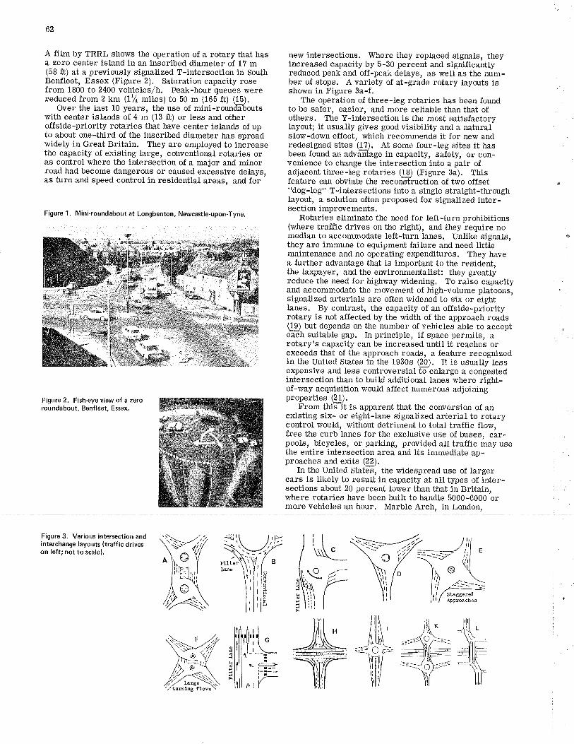
62
A film by TRRL shows the operation of a rotary that hasa zero center island in a¡ inscribed diameter of 1? m(58 ft) at a previously signalized T-intersection in SouthBenfloot, Essex (Figure 2), Saturation capacity rosefrom 1800 to 2400 vehicles,/h. Peak-hour queues werereduced from 2 km (1% miles) to 50 m (165 ft) qÐ.
Over the last 10 years, the use of mini-roundaboutswith center islands of 4 m (13 ft) or less and otheroffside-priority rotaries that have center islands of upto about one-third of the inscribed diameter has spreadwidely in Great Britain. They are employed to increasethe capacity of existing large, cohventional rotaries oras control where the intersection of a major ard minorroad had become dangerous or caused excessive delays,as turn and speed control in residential areas, and for
Figure 1. Mini-roundabout at Longbenton, Newcastle-upon-Tyne.
Figure 2. Fishcye view oÍ a zeroroundabout, Benf leet. Essex,
new intersections. Where they replaced signals, theyincreased capacity by 5-30 percent and significantlyreduced peak and off-peak delays, as well as the num-ber of stops. A variety of at-grade rotary tayouts isshown in Figure 3a-f.
The operation of three-leg rotaries has been foundto be safer, easier, and more reliable than that ofothers. The Y-intersection is the most satisfactorylayout; it usually gives good visibility and a naturalslow-down effect, which recommends it for new andredesigned sites (1?). At some four-leg sites it hasbeen found an advantage in capacity, sa-tety, or con-venience to change the intersection into a pair ofadjacent three-leg rotaries (18) (Figure 3a). Thisfeature can obviate the recons-truction of two olfset"dog-leg" T-intersections into a single straight-throughlayout, a solution often proposed for signalized inter-section improvements.
Rotaries eliminate the need for left-turn prohibitions(where tra-tfic drives on tlre right), and they require nomedian to accommodate left-turn lanes. Unlike sígnals,they are immune to equipment failure and need littlemaintenanse and no operating ex¡lenditures. They havea further advantage that ís important to the resident,the ta4payer, and the environmentalist: they greatlyreduce the need for highway widening. To raise capacityand accommodate the movement of high-volume platoons,signalized arterials are often widened to six or eightlanes. By contrast, the capacity of an offside-priorityrotary is not affected by the width of the approach roads[!) but depends on the number of vehícles able to accepteach suitable gap. In principle, if space permits, arotary's capacity can be increased until it reaches orexceeds that of the approach roads, a feature recognizedin the United States in the 1930s eg). It is usually lessexpensive and less controversial to enlarge a congestedintersection than to build additional lanes where right-of-way acquisition would affect numerous adjoiningproperties (21).
From this it is apparent tlrat the conversion of anexisting six- or eight-lane signalized arterial to rotarycontrol would, without detriment to total traffic flow,free the curb lanes for the exclusive use of buses, car-pools, bicycles, or parking, provided all tra-ffic may usethe entire intersection area and its immediate ap-proaches and exits (??).
In the United States, the widespread use of largercars is likely to result in capacity at all types of inter-sections about 20 percent lower than tùat in Britain,where rotaries have been built to handte 5000-6000 ormore vehicles an hour. Marble Arch, in London,
Figure 3. Various intersection andinterchange layouts (traff ic driveson left; not to scale).
sH
F11ter
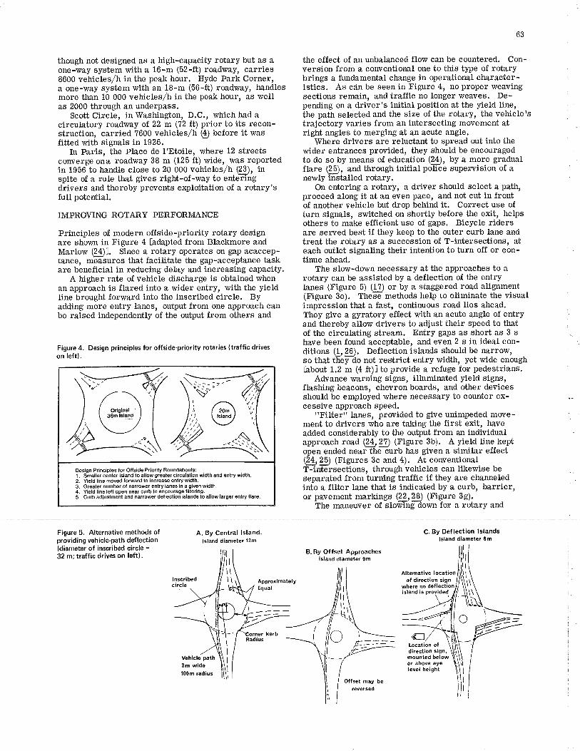
though not designed as a high-capacity rotary but as aone-way system with a 16-m (52-ft) roadway, carries8600 vehicles/h in the peak hour. Hyde Park Corner,a one-way system with an 18-m (56-ft) roadway, handlesmore than 10 000 vehicles/h in the peak hour, as weIIas 2000 through an underpass.
Scott Circle, in Washington, D.C., which had acirculatory roadway oÎ.22 m (?2 ft) prior to its recon-struction, carried ?600 vehicles/h (Ð before it wasfitted with signals in 1926.
In Paris, the Ptace de I'Etoile, where 12 streetsconverge ona roadway 38 m (125 ft) wide, was reportedin 1956 to handle close to 20 000 vehicles/h €Ð, inspite of a rule that gives right-of-way to enteringdrivers and thereby prevents exploitation of a rotary'sfull potential.
IMPROVING ROTARY PERFORMANCE
Principles of modern offside-priority rotary designare shown in Figure 4 hdapted from Blackmore andMarlow (?ÐJ. Since a rotary operates on gap acaccep-tance, measures that facilítate the gap-acceptance taskare benefieial in reducing delay and increasing capacity.
A higher rate of vehicle discharge is obtained whenan approach is flared into a wider entry, with the yieldline brought forward into the inscriloed circle. Byadding more entry lanes, output from one approach canbe raised independently of the output from others and
Figure 4. Design principles for offside-priority rotar¡es (traffic driveson left).
63
the effect of an unbal;anced flow can be countered. Con-version from a conventional one to ttris t¡pe of rotarybrings a fundamental change in operational character-istics. As c¿in be seen in Figure 4, no proper weavingsections remain, and tra-ffic no longer weaves. De-pending on a driver's Ínitial position at the yield line,the path selected and the size of the rotary, the vehicle'strajectory varies from an intersecting movement atright angles to merging at an acute angle.
Where drivers are reluctant to spread out into thewider entrances provided, they should be encouragedto do so by means of education (?4), by a more gradualflare (25), and through initial police supervision of anewly installed rotary.
On entering a rotary, a driver should select a path,proceed along it at an even pace, and not cut in frontof another vehicle but drop behind it. Correct use ofturn signals, switched on shortly before the exit, helpsothers to make efTicient use of gaps. Bicycle ridersare served best if they keep to the outer curb lane andtreat the rotary as a succession of T-intersections, ateach outlet signaling ttreir intention to turn off or con-tinue ahead.
The slow-down necessary at the approaches to arotary can be assisted by a deflection of the entrylanes (Figure 5) É.!) or by a staggered road alignment(Figure 3e). These methods help to eliminate the visualimpression that a fast, continuous road lies ahead.They give a gyratory effect with an acute angle of entryand thereby allow drivers to adjust their speed to thatof ttre circulating stream. Entry gaps as short as 3 shave been found acceptable, and even 2 s in ideal con-ditions (1,26). Deflection islands should be narrow,so that t-treÍäo not restrict entry width, yet wide enoughhbout 1.2 m (a ft)l to provide a refuge for pedestrians.
Advance warning signs, illuminated yield signs,flashing beacons, chevron boards, and other devicesshould be employed where nesessary to counter ex-cessive approach speed.
"Filter" lanes, provided to give unimpeded move-ment to drivers who are taking the first exit, haveadded considerably to the output from an individualapproach road €4, Ð (Figure 3b). A yield line keptopen ended near the curb has given a similar effect1232j) (Figures 3c and 4). At co¡¡ventionalT-intersections, through vehicles can likervise beseparated from turning tra-ffic if they are channeledinto a filter lane that is indicated by a curb, barrier,or pavement markings (U,29 (Figure 3g).
The maneuver of slowing down for a rotary and
r-,)qï7
Dæign Principles for Offside Pr¡orily Roundabouts:1 . Smaller center ¡sland to allow gteater c¡rculal¡on wldth 8nd entry width.2. Yield l¡ne moved Joruard to ¡ncrease entry w¡dth.3. Greater number ol nar¡ower entry lanos in a given width,4. Y¡eld line lelt open near curb to encourage lilt6r¡ng.5. Curb adiustment and narrower deflætion islands lo allow lsrger entry tlare.
Figure 5. Alternative methods ofproviding vehicle-path def lection(diameter of inscribed circle =32 m; traffic drives on left),
A. By Central lsland,lsland d¡ameter t2m
C. By Deflection lslandslsland d¡amstCr 6m
B. By Offset Approacheslsland diameter 9m
Ir
fi\
Alternâlive local¡onof dirclion
where no deflêc
Locåt¡on old¡rection s¡gn,
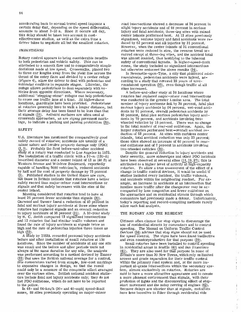
64
accelerating back to normal travel speed imposes acertain delay tiat, depending on the speed differential,amounts to about 2-10 s. Since it occurs all day,
road intersections showed a decrease of 34 percent inslight injury accidents and of 46 percent in seriousinjury and fatal accidents; three-Ieg sites with raised
efÏectiveness studies, as well as the extra time adriver takes to negotiate all but the smallest rotaries.
PEDESTRIANS
Rotary control appears to bring considerable benefitsto both pedestrian and vehicle sa-fety, This can beattributed to a smooth flow and to comparatively simpledecisions made at low speed. Crosswalks, ptaced twoto three car lengths away from the yield line across thethroat of the entry flare and divided by a center refuge(Figure 4), allow the driver to deal with pedestrian andvehicular conflicts in separate stages. Likewise, therefuge allows pedestrians to deal separately with ve-hicles from opposite directions. Wrere necessary,additional " stepping- stone " refu ge s can help pede striansto cross one tra-tfic lane at a time, At high-volumelocations, guardrails have been provided. Pedestriansat rotaries generally have to walk a longer distance, buttheir average delay has been found to be less than thatat signals (19). Aniiskid surfaces are often used atcrosswalk approaches, as are zigzag pavement mark-ings, to indicate a parking and passing prohibition (?9).
SAFETY
U.S. literature has mentioned the comparatively goodsa-fety record of rotaries; accidents are usually of aminor nature and involve property damage only (PDO)(å Ð. Probably the first before-and-a-tter accidentstudy at a rotary was conducted in Los Angeles in L922.The installation of a tra-ffic circle with a37-m (120-ft)inscribed diameter and a center island of 12 m (40 ft) atWestern Avenue and Wilshire Boulevard, reportedlycapable of handling 5000 vehicles,/h, reduced accidentsby half and the cost of property damage by 75 percent(Ð. Published studies in the United SLates are rare,but those in BrÍtain indicate that rotaries have a bettersa-fety record than major-minor road intersections orsignals a¡d that safety increases with the size of thecenter island.
Manning considered that rotaries tend to have atleast 25 percent fewer accidents than signals (30).Garwood and Tanner found a reduction of 83 percent infatal and serious injury accidents at three sites whererotaries had replaced signals and an overall reductionin injury accidents of ã6 percent (.31). A l0-year study THE ROTARY AND THE RESIDENTby If. C. Smiffircompãreã 12 sigffizeA intersections
signalized, serious injury and fatal accidents were re-duced by 62 percent and all injuries by 31 percent.However, when the center islands of 31 conventionalrotaries were reduced in size, the reverse trend oc-curred except at t¡ree-leg sites, and tl¡e accident totalwas almost doubled, thus testifying to the inherentsafety of conventional layouts. In higher-speed-Iimitzones, the study included no signalized intersectionsbut otherwise endorsed the above results GÐ.
In Newcastle-upon-Tyne, a city that pioneered mini-roundabouts, pedestrian accidents were halved, ac-cording to a study tlrat covered 22 years of mini-roundabout operation (Ð, even though tra-ffic at allsites increased.
A before-and-after study at 38 locations whererotaries had replaced major-minor road intersectionswas conducted in tlre greater London area. The totalnumber of injury accidents fell by 39 percent, fatal plusserious injury accidents by 64 percent, wet-road acci-dents by 51 percent, overall pedestrian accidents by46 percent, fatal plus serious pedestrian injury acci-dents by 70 percent, and accidents involving two-wheeled vehicles by 18 percent. There was no chångein the total number of rear-end collisions. Again, theLarger rotaries performed best-overall accident re-duction of 52 percent. At sites with curbless centerislands, total accident reduction was only 23 percent;these sites showed an increase of 60 percent in rear-end collisions and of ? percent in accidents involvingtwo-wheeled vehicles (t9).
Despite the general reduction in injury accidents andtheir severity, more sideswipes and other PDO incidentshave been observed at several sites (14, 19,Ð; this isattributed to a higher level of activity at high-capacityrotaries, To allow a true assessment of the effect of achange in tra-ffic control devices, it would be useful ifstudies included every incident, the tra-ffic volumes,and accidents within the neighboring roadnet. For ex-ample, an increase in accidents at an intersection thathandles more tra-ffic a-fter the changeover may be ac-companied by less congestion and fewer collisions onthe approaches and on residential streets through whichcommuters had previously made a detour. Unfortunately,today's reporting and record-compiling methods rarelyallow such full analysis.
and 12 rotaries that had similar tra-ffic volumes andfound the rate of injury accidents at signals twice ashigh and the rate of pedestrian injuries three times asnieh (9Ð.
A study by TRRL recorded personal injury accidentsbefore and after installation of small rotaries at 150locations. Since the number of accidents at any one site
tics include fatal and injury accidents only; they do notlist PDO collisions, which do not l¡ave to be reportedto the police.
In 48- and 64-km/h (30- and 40-mph) speed-limitzones, 88 sites previously operating as major-minor
Citizens often clamor for stop signs to discourage theuse of residentíal streets by commuters and to controlspeeding. The Manual on Uniform Tra-ffic ControlDevices L3B) advises that stop signs shouLd not be usedfor speed control. The signs have been found ineffectiveand even counterproductive for that purpose (39).
Small rotaries have been installed to contrõÍ speedingwas small and the before and after periods were not in residential areas in Seattle É9 ard San Franciscoalways of the same duration for any site, the analysis (41). They are also used for tffi purpose in some ofwas performed according to a method devised by Tanner Éätain's more than 30 New Tolns, which rely onlimited€Ð that uses the British national average for a control. access and grade separation for their tra-ffic controlSite conversions varied from simple, Iow-cost markings within the primary road system and, at the more im-to e4pensive changes in design, so that the result portant at-grade intersections within the secondary sys-could only be a measure of the composite effect averaged tem, almost exclusively on rotaries. Rotaries areover the various sites. British national accident statis- said to have a more attractive appearance and to create
a more pleasant environment than signals, with theirprofusion of lights and the disconcerting efTect of stop-start movement and the noisy rewing of engines (42).Because delays are shorter than at signals, motoristshave less incentive to filter through residential side
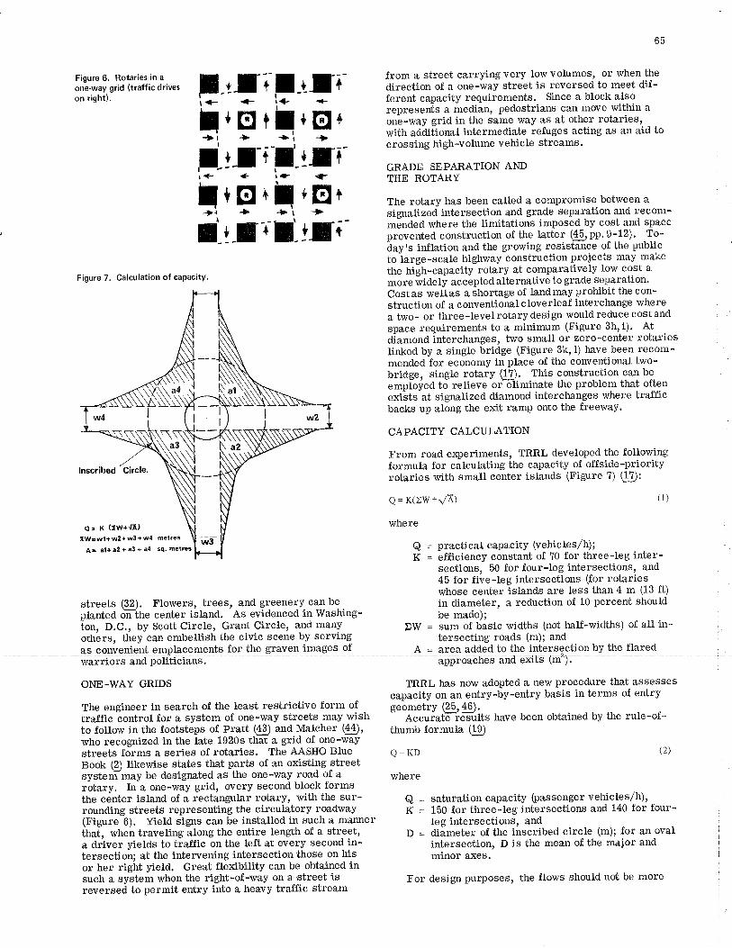
Figure 6. Rotar¡es in aone-way grid (traffic driveson right).
I r-r r^-i+- <- l<- <-
f '9'l'9't-rf-il.tf{-r<É- + t* +
f t@ii-Etriirrl:tr'i-
65
from a street carrying very low volumes, or when thedirection of a one-way street is reversed to meet dif-ferent capacity requirements. Since a block alsorepresents a median, pedestrians can move within aonè-way grid in the same way as at other rotaries,with additior¡al intermediate refuges acting as an aid tocrossing high-volume vehicle streams.
GRADE SEPARATION ANDTHE ROTARY
The rotary has been called a compromise between asignalized intersection and grade separation and recom-mãnded where the limitations imposed by cost and spaceprevented construction of the latter GÐ pp.9-12). To-ãay's inftation a¡rd the growing resistance of the publicto-Large-scale highway construction proiects may ma}ethe hiáh-capacity rotary at comparatively low cost a
more ioidety accepted alternative to grade separation'Cost as well as a shortage of land may prohibit the con-s truction of a c onventi onal c love rlea-t inte rchange whe rea two- or three -level rotary design would reduce cost and
space requirements to a minimum (Figure 3h'i). Aldiamond interchanges, two small or zero-center rotariesLinked by a single bridge (Figure 3k, 1) have been recom-mended for economy in place of the conventional two-bridge, single rotary (1?). This construction can be
empioie¿ tõ re[eve or-lliminate the problem that oftenexists at signatized diamond interchanges where tra-fficbacks up along the exit ramp onto tJle freeway.
CAPACITY CALCULATION
From road e4periments, TRRL developed the followingformula for calculating the capacity of ofTside-priorityrotaries v¡ith small center islands (Figure 7) qf):
q = r1:w +/Ã)
where
0)
streets (!Ð, Flowers, trees, .and greenery. can beptanted oî-the center island. As evidenced in Washing-ton, D.C., by Scott Circle, Grant Circle, and many ÞW =others, they can embeltish the civic scene by serving
= practical capacity (vehictes/h);efÏiciency constant of ?0 for tlree-leg inter-sections, 50 for four-leg intersections, and45 for five-leg intersections (for rotarieswhose center isl,ands are less than 4 m (13 ft)in diameter, a reduction of 10 percent shouldbe made);sum of basic widths (not half-widths) of all in-tersecting roads (m); and
aK
Figure 7. Calculation of capacity.
a¡ K (tw+{Ã)tw.wttw2+w3+w¿l m"ttc3
A. ¡l+ a2 + å3 + âl !q. mettcs
ONE-WAY GRIDS
The engineer ín search of the least restrictive form oftra-ffic ãontrol for a system of one-way streets may wishto follow in the footsteps of Pratt €X) and Malcher Q!)'who recognized in the late 1920s that a grid of one-waystreets forms a series of rotaries. The AASHO BlueBook (2) likewise states tftat parts of aa existing streetsysterñmay be desigrrated as the one-way road of arôtary. In a one-way grid, every second block formsthe center island of a rectangular rotary, with tlte sur-rounding streets representing the circulatory roadway(Figure 6). Yield signs ca¡ be installed in such a marulerthat, when travelíng along the entire length of a street,a driver yields to tra-ffic on the left at every second in-tersection; at the intervening intersection those on hisor her right yield. Great flexibility can be obtained insuch a system when the right-of-way on a street isreversed to permit entry into a heavy tra-tfic stream
TRRL has now adopted a new procedure that assessescapacity on an entry-by-entry basis in terms of entrygeometry (?9r!Ð.- Accuiatã1e-zults have been obtained by the rule-of-thumb formuta (!$
Q=KD (2)
where
= saturation capacity þassenger vehicles,/h),= 150 for three-leg intersections and 140 for four-
leg intersections, and
= diámeter of the inscribed circle (m); for an ovalintersection, D is the mean of the major andminor axes.
aK
D
For design purposes, tJ:e flows should not be more
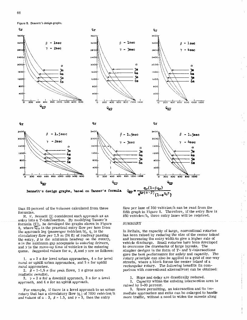
66
Figure 8. Bennett's design graPhs.
qr
QEI'
qrqlqr
ß
"l
- l.Jecc
- 2e¿c
a<þ IOOO l2OO l,loo lóOO
ûþl+.uh
aoo óoo
cEP
Bcnnett's ileetgn
aoo aoo tooo reoo
QEI,
gra¡ùre, basod on Tan¡¡er's for¡r¡lr b.
than 85 percent of the volumes calculated from these flow per lane of 350 veNcles /h can be read from theformulas. fifth graph in Figure 8. Therefore, if the entry flow is
R. F. Bennett Q considered each approach as an 850 vehictes/h, three entry lanes will be required.entry into a T-intersection. By modifying Tanner'sformula (4?), he developed the graphs shown in Figure SUMMARYB, where Q-¡p is the practical entry florr per lane fromttie approaôtr leg þalsenger vehieles,/h), q. is the In Britain, the capacity of large, conventíonal rotariescircu-iàtorv flow pãr 7.5 m (24 ft) of roadwáy passing has been raised by reducing the size of tlte center islandcirculatory flow per 7.5 m (24 ft) of roadway passing has þeen raisect by rectucing tne srze or fne ceruer ls,
the entry, -B
is tlie minimum heâdway on the rotary, and increasing the entry width to give a higher rate ofa is the
-minimum gap acceptable to entering drivers, vehicle discharge. SmaII rotaries have been developed
and 7 is the move -up time õf vehicles in the entering to overcome the drawbacks of large layouts. Thequeue. Suggestedvàlues for a, B,andTare as foUows: simpler designs inthe form of T- andY-intersections
gave the best performance for sa-fety and capacity. The
1. e= 3 s for levelurbanapproaches, 4 s for level rotaryprinciple canals^obe appliedtoa gridof one-wayrural or uphill urban approachôå, and 6 é for uphill streets, where. a block forms the center isÞnd of arural apprìaches. rectangular rotary. The f.ülowing benefits (in com-
2. i-= f -f .O s (for peak flows, 1 s gives more parison with conventional alternatives) can be obtained:
realistic results).B. f=2sfoiadownhillapproach,3sforalevel 1. Stopsanddeliayaredrasticallyreduced.
app"oaäh, and 4 s for an uphiiliapproách. 2, Capacity within the existing intersection area israised bY 5-30 Percent.
For example, if there is a level approach to an urban 3. Sþace permitting, an intersection and its im-rotary that has â circulatory flow (q.) of 1600 vehicles/h mediate approaches and exits can be enlarged to handle
and vähes of a = 3, Ê = L,5; and 7'='i, then the entry more tra-tfic, without a need to widen the streets along
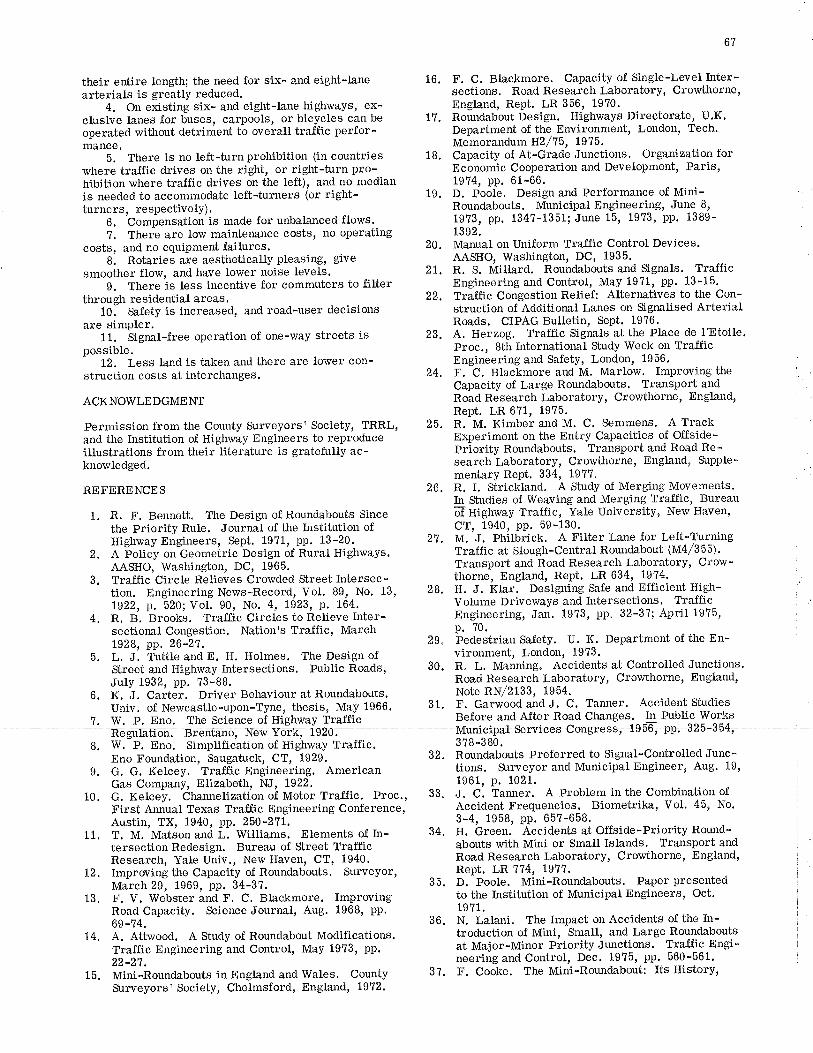
l. Yv. r. s¡¡u. ¡¡¡v wrv¡¡vv vÀ ¡¡¡õ¡^rY4J
-
nicipal services gongress,{956, pp;3*5-38+,8. 'tr.-P. Eno. Simplifióation of Higihway Traffic. 378-380'
6',1
their entire lengfh; the need for six- and eight-tane 16. F. C. Blackmore. Capacity of Single-Level Inter-arterials is greãtti reduced. sections. Road Research Laboratory, Crowthorne,
4. On eãsting six, and eight-lane highways, ex- Engl;and, Re¡t. IR 356., .1970.clusive lanes for buses, carpoõb, or bicycles can be L7. Roundabout Design. Highways Directoratc, U.K.operated without detriment to oveialt traúic perfor- Department of the Environment, London, Tech.mance. -
Memorandum H2/15t L975.
b. There is no left-turn prohibition (in countries 18. Capacity of At-Grade Junctions. Organization forwhere tra-tfic drives on the right, or right-turn pro- Economic Cooperation and Development, Paris,hibition where tra.ffic drives on the left), and no median 19?4, pp. 61-66.is needed to accommodate left-turners'(or right- 19. D. Poole. Design and Performance of Mini-lu"""rÀ, respectively). Roundabouts. Municipat Engineeri,ng, June- 8,
O. 'Compensation'is made for unbalanced flows. 1973, pp. 134?-1351; June 15, 19?3, pp. 1389-
1. Therì are low maintenance costs, no operating 1392'
costs, ano no equipment failures. 20. Ma¡rual on Uniform Tra-ffic Control Devices.
8: RotarieJ aie aesthetically pleasing, give AASIIO, Washington, DC, 1935.- --
smoother flow, and have lower nôièe teveiÁ. 2L, R. s. Miltard. Roundabouts and signals. Tra-tfieg. There is less incentive for commuters to filter Engneering and Control, May 19?1, pp. 13-15.-
through residential areas. 22, Tra-tfic Congestion Relief: Alternatives to the Con-
1ol satety is increased, and road-user decisions struction of Additional Lanes on Signalised Arterialare simpler. Roads. CIPAG lulletin, sept. 1976.
11. 'S\gr¡al-free operation of one-way streets is 23. A. Herzog. Tra^ffic Signâls at the Place de lrEtoile.possible. Proc., 8th International Sbudy Week on Traffic
t2, Less land is taken and there are lower con- Engineering and Safety, Londoa, 1956.
struction costs at interchanges . 24. F. C. Blackmore and M. Marlolv. Improving theCapacity of Large Roundabouts. Transport and
ACKNOWLEDGMENT Road Research Laboratory, Crowthorne, England,RePt. LR 671, 1975.
permission from the County Surveyors' Society, TRRL, 25, R. M. Kimber and M. C. Semmens. A Trackand the Institution of Hishwäy Engineers to reploduce Experiment on the Entry- Capacities of offside-illustrations from greir"Iiteräturõ is gratefully ac- Priority Roundabouts_. Transport and Road Re-knowledged. search Laboratory, Crowthorne, Engl,;and, Supple-
REFEREN.ES 26. ffi:åi"*ithÍl-itriil; or Merging Movemenrs.In Studies of lVeaving and Merging Tra-tfic, Bureau
1. R. F. Bennett. The Design of Roundabouts Since õTnighway Traffic,.-Yale University, New Haven,
the Priority Rule. Journal of the Institution of CT, 1940, Bp.' 59'130'.-Highway Engineers, Sept. 19?1, pp. 13-20. 27. M. J. Philbrick. A Filter Lane for Left-Turning
2. A policy on Geometric Design of Rural Highways. Traffic at Slough-Central Roundabout (M4/355).
AAsHo; Washington, DC, 1õ6b. Transport and load Research Laboratory, Crow-3. TratTic Circle Relieves irowded Street Intersec- thorne, England, .ne.nt' -l'! 634, tg74'
tion. Engineering News-Record, Vol. 89, No. 13, 28. I. J. Klar. Designing Safe and Efficient High-
l9zz, p. *szo;
voti ï0, ¡lo. 4, ró2g, p. ró+. volume Driveways and Intersections. Tra-ffic
4. R. B. Brooks. Traffic Circles to Relieve Inter- Engineering, Jan. 1973, pp' 32-37; April 1975,
sectional Congestion. Nation's Tra-ffic, March p' 70'
iOZe, pp. 26:27.--'-' ' 29, Pedestrian Sa-fety. U. K. Department of the En-
5. L. J. Tuttle and E. H. Holmes. The Design of vironment, London, 19?3.
Street a¡rd Highway Intersections. public ñoads, 30. R. L. Manning. Accidents at Controlled Junctions.
July 1982, ppl Zg-gg. Road Research Laboratory, Crowthorne, England,
6. K. J. Carter. Driver Behaviour at Roundabouts. Note RN/2133, 1954"
Univ. of Newcastle-upon-Tyne, thesis, May 1966. 31. F. Garwood ald J. C. Tanner. Accident Studies
7. W. p. Eno. The Sciônce oi Hígtrway'iratfic Before and After Road Changes-. -þ PubliS^pgrt<s
Traffic at Slough-Central Roundabout (M4/3 55).Transport and Road Research Laboratory, Crow-thorne, England, RePt. LR 634, t974.H. J. Klar. Designing Safe and Efficient High-Volume Driveways and Intersections. Tra-fficEngineering, Jan. 1973, pp. 32-37; April 1975,p.70.
29, Pedestrian Sa-fety. U. K. Department of the En-vironment, London, 19?3.
30. R. L. Manning. Accidents at Controlled Junctions.Road Research Laboratory, Crowthorne, England,Note RN/2133, 1954"
31. F. Garwood atd J. C. Tanner. Accident Shdies
Eno Foundation, Saugatuck, CT, 1929. 32. Roundabouts Preferred to Signal-Controlled Junc-9. G. G. Kelcey. Traffic Engineering. American
Gas Company, Elizabeth, NJ, 1922.10. G. Kelcey. ótra¡rneuzation oi Motor Tra-ffic. Proc., 33.
First Annual Texas Tra^ffic Engineering Conference,Austin, TX, 1940, pp. 250-271.
11. T. M. MatÁon and i, Williams. Elements of In- 34.
tersection Redesign, Bureau of Street Tra^fficResearch, Yale Univ., New Haven, CT, 1940.Improving the Capacity of Roundabouts. Surveyor,March 29, 1969, pp. 34-37.F. V. Webster and F. C. Bþckmore. ImprovingRoad Capacity. Science Journal, Aug. 1968, pp.69-74.A. Attwood. A Siudy of Roundabout Modifications.Traffic Engineering and Control, May 1973, pp.22-21.Mini-Roundabouts in England and Wales. CountySurveyors' Society, Chelmsford, England, 1972.
tions. Surveyor and Municipal Engineer, Aug. 19,
1961, p. 1021.J. C. Tanner. A Problem in the Combination ofAccident Frequencies. Biometrika, Vol. 45, No.3-4, 1958, pp. 657-658.H. Green. Accidents at Offside-Priority Round-abouts with Mini or Small Islands. Transport andRoad Research Laboratory, Crowthorne, England,Rept. LR 114, 19'17.D. Poole. Mini-Roundabouts. Paper presentedto the l¡rstitution of Municipal Engineers, Oct.19?1.N, Latani. The Impact on Accidents of the I¡-troduction of Mini, Small, and Large Roundaboutsat Major-Minor Priority Junctions. Traffic Engi-neering and Control, Dec. 1975, pp. 560-561.F. Cooke. The Mini-Roundabout: Its History'
t2.
13.
L4.
35.
36.
15. 3?.
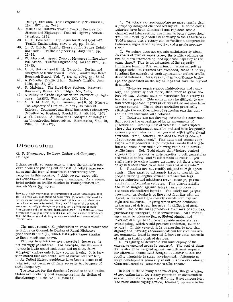
6B
44. F. Malcher. The Steadyflow System. Harvard g. "Rotaries require more right-of-way and road-University Press, Cambridge, MA, 1935. way, and generally cost more, than other at-grade in-
45. A Policy on Grade Separation for Intersecting High- tersections. Access must be controlled for frotary toways. 4AS_|1O, Washington, DC, 1544, function properly. This control may be difficult to ôb-46. M. G. M. Glen, S. L. Sumner, and R. M, Kimber. ¡¿in wheñ approãch highways or streets do not also haveThe Capacity of OfÏside-Priority Roundabout access control.,' Theðe characteristics practicaltyEntries. Transport and Road Research L,aboratory, eliminate the consideration of replacing èxisting higil-Crowthorne, England, Special Rept. SR 436, 1979. volume intersections with rotaries.
41. J. C. Ta¡ner. A Theoretical Analysis of Delay at 4, "Rotaries are not directly suitable for conditionsar Uncontrolled Intersection. Biometrika, Vol. 49, that require the crossings of Laige movements of1962, pp. 163-170. pedestrians. Orderly flãw of vehicles is interrupted
where this requirement must be met and it is frequantlynecessary for rotaries to be operated with traffic signalcontrols, This, however, violates the rotary conceptof continuous movement." This statement seems very
Discussion iifiï¡i"-:i1'":"i;..:,1iffål;"JjÏffJil'ffi'S'TTJ'"îätra-ffic lanes. Yet, Todd states that "Rotary control
G. F. Hagenauer, De Leuw Cather and Companyt àppears to bring considerable benefits to both pedestrianChicago añã vehicle saJety" and "Pedestrians at rotaries gen-
erally have to walk a longer distance, but their averageI think we all, to some extent, shâ.re the author's con- delay has been found to be less than ihat at signals."cern about the phasing out of existing rotary intersec- b. "Rotaries are not readily adapted to high-speedtions a¡d the lack of interest in constructing new roads. They must be extremeiy large to provide therotaries in this country. I think we can agree with proper weaving lengths between inteisectibn legs.his assessment of their many advantages. As a recent Large rotaries add additional travel mileage, partic-brief article on traffic circles in Transportation Re- ubrly for left-turning vehicles. This characteristicsearch News (49) noted, should be weighed agáinst delays likely to occur at
alternate channelized layouts. For saJety and properln view of their many apparent advantages, it would seem logical that operation, particularly of t¡oSe not familiar with üretrafficcircleswouldcontinuetobeuniversallypopular. Theneedfor byout, nú*ero.rssignSclearlyvisiblebothdayandexpensive and complicated conventional traffic control devices may ;:;; l-^;:-:;;:r--ï;:;::-.,'"rr;;;.,:,;:-;be reduced or even etiminated. The graceful lines of circles would night are essential. Signing which avoids confusionseem aesthetically preferable to the angularity of typical at-grade on the part of drivers, however, is difficult of attain-i¡relseeûorrr añd their corrtÍol h-rdwãaé-luttétl The contÍñuoutflõw menffiOne oÊthernan¡problems foruSersof=otaries,of vehicles through a circle provides a quieter and cleaner environment particularly strangers, is disorientation. As a result,than the stopping and starting actions associated with conventional care must be taken so that sufficient signing andintersections. marking is supplied to properly guide motoiists; yet
rhe mosr recenr u.s. pubricarion in rodd's rererences ;i:tT;å:t? riiT"ååäÏ#i"tifå""""#i-'?å'ri:"ril;is Policy on Geometric Design of Rural Highways, signing and marking recommendations for rotaries arepublished in 1965 (Ð, which lists advantages similar not commonly found in current federal or state manualsto those mentioned above. of uniform tra-ffic control devices.
Design, and Use. Civil Engineering Technician,Nov. 19?3, pp. 7-23.
38. Manual on Uniform Tra-ffic Control Devices forStreets and Highways. Federal Highway Admin-istration, 1978.
39. R. F. Beaubien. Stop Sigrrs for Speed Control?Tra^ffic Engineering, Nov. 1976, pp. 26-28.
40. L. C. Orlob, Tra-ffic Diversion for Better Neigh-borhoods. Tra-tfic Engineering, July 19?5, pp.22-25.
4L. W. Marconi. Speed Control Measures in Residen-tial Areas. Traffic Engineering, March 1977, pp.28-30.
42. C. B. Horman and H. H. Tt¡rnbull, Design andAnalysis of Roundabouts. Proc., Australian RoadResearch Board, Vol. 7, No. 4, 19?4, pp. 58-82.
43. A Proposed Tra-ffic PIan. Nation's Traffic, June1929, pp. 31, 37.
1. 'rA rotary can accommodate no more traffic thana properly designed channelized layout. In some cases,rotaries have been elimirlated and replaced with acharmelized intersection, resulting in better operation."This statement by AASHO is contrary to the assertion inTodd's paper tìat a rotary can be "called a compromisebetween a signalized intersection and a grade separa-tion."
2. "A rotary does not operate satisfactorÍly when,on roads of four or more lanes, the tra-tfic volumes ontwo or more intersecting legs approach capacity at thesame time." This is an extension of the capacityIimitation found in U.S. e4perience. When capacitiesof approaches to rotaries are exceeded, there is no wayto adjust the capacity of each approach to reflect tra,fficdemand volumes. As a result, disproportionate back-ups are generated on the leg or legs that have the highestdemands,
6. "Lighting is desirable and landscaping of theextensive unpaved areas is required. The cost of theseitems should be weighed against installations requiredfor alternate charineüzed designs, . . . Rotaries are notreadily adaptable to stage development. Attempts atstage development generally result in some over-designwhen measured by immediate tra-ffic needs."
The way in which they are described, however, isnot strongly persuasive. For example, the statement"the¡e is little speed reduction and no delay fromstopping" applies only to low volume levels. It is fur-ther stated tJlat accidents "are of minor nature" but,in the United States, accidents have been a concern atrotaries, not because of their severity but because oftheir frequency.
The reasons for the demise of rotaries in the United In light of these many disadvantages, the generatingStates are probably best summarized in the listing of of new enthusiasm for rotary retention or constructiondisadvantages in the AASHO Manual: in the United States appears difficult, if not impossible.
The most discouraging advice, however, appears in the
69
report of the Committee on Urban Street Design of tlre in advance of the circle in order to meter the flow intoInstitute of Transportation Engineers (ITE). Íhe re- the circle. Since this approach used no additional right-port, Guideunes fìr Urban uajor sf¡eet nesign, is of-way, it does not disturb the land use adiacent to the
described as "a proposed recommended practice"; it is circle, nor does it involve lengthy and complicated con-in tÌre final stages of review and approval by ITE's struction.Technical Council and Board of Direction. Rotary in- Since tra"ffic circles in our state tend to be the
tersections are mentioned on only one page of this very preferred locations for gasoline stations, shopping cen-Iarge report: ,'rotary intersections are not recom- ters, and diners, the Last item_is not a minor one. We
mended....Rotaries are undesirable because of the have at present one circle that has five approach road-high number of weaving movements that must be ac-commodated in a short distance."
It would appear that the handwriting has been on thewall for quite a few years. Todd's paper is based onextensive references from both the United States andoverseas. The latter, however, are mostly fromGreat Britain, where rotaries have been uniquelysuccessful. Those from this country, on the otherhand, are principally from the years prior to 1940, andtheir applicability to present conditions can be ques-tioned.
Since at least the 1960s, however, U.S. engineerson the state and local levels and consultants have beenworking to produce good operation in existing rotaries Jack E. Leisch, Jack E. Leisch and Associates,and, based on their e¡perience, have recommended Evanston, Illinoisthat new rotaries should not be constructed. In theface of these facts, a resurgence of interest in rotaries Todd's paper is an enlightening account of the designin this country *oúld s"u* extremely unlikely. and operation of rotary intersections in Great Britain.
Normally the subject would draw little interest in the
REFERENCE UNiTCd StAtES.The rotary as a real tra-ffic carrier has been written
48, Tra-ffic Circles: Their Past, Present, and Future.Transportatíon Research News, Sept. -Oct. 19?Btpp. 4-6.
have been used to replace tra.ffic signals. This is iustopposite to our practice. 'vVe have reconstructed anumber of circles by cutting through them and signaliz-
ways, all signalized, with detectors in both the ap-proach roadways a¡d the circle proper, wired into aèomputer instatled in a trailer inside the circle. Studiesnow under way at that location, Ellisburg Circle, showthat we can achieve total hourly volumes in excess of4000 vehicles/tr but that above 4400 vehicles/h the flowtends to become unstable and "Iockups" occur beyondthat point.
off and, for the most part, considered a relic inmodern transportation engineering practice in theUnited States. Of course, the rotary may have itsplace for local or distributor-type tra-ffic at low volumesior aesthetic or architectural purposes and occasionallyfor maintaining low speed levels in residential com-munities. Such minor use, however, is incidental,since this discussion focuses on situations where theability and necessity to handle tra-tfic is of primaryconcern.
Although this paper at first glance may not seemrelevant, it does command interest and perhaps someanalysis because of the unusually optimistic and highlyfavorable account presented in terms of increasedcapacity, operational efficiency, safety, and a multitude
the past 10 years. Their adva¡rtage is that the capacityhas been increased 50 percent by means of reducingthe size of the center island (of previous designs) andincreasing the entrY wÌdth.
Atthough it is assumed that such design and attendantperformance could not be achieved and certainly wouldnot be attempted in the United States, we must recognizethat Todd's presentation draws on actual e4perienceand research, and it consequently deserves properattention. There must be an ex¡llanation for suchdiversity in design application and operatio¡ral ex-
Robert J. Nolan, Bureau of Tra^ffic Engineering,New Jersey Department of Transportation,Trenton
Although the New Jersey Department of Transportationis not constructing any new circles on its highway sys-tem, we do have approximately 60 circles o_n our sys-temj most of ttrembuilt in the 1920s and 1930s. No one of other advantages attributed to the use of rotaries inis advocating building any more. Therefore, insofar Great Britain. The troublesome aspect of this reviewas our highway system ié concerned, the basic problem is that nearly every performa¡ce level or characteristicis not how to design new trarfic circles but what is the cited as an attribute and an advantage for the Britishbest approach to improve the operation of those we have. situation is considered a failure and a disadvantage for
Todd states that, in somliAccording to our experience in the United States, it
is hard to conceive that rotaries could improve safety,lessen delays, and reduce pedestrian-vehicular hazards
ing the resulting intórsectiõns. Wé have found that such What is realty difficult to comprehend is that "mini-a technique results in a smoother flow, witlr less con- roundabouts" with center islands less than 4 m (13 ft)gestion -¿ t"* accidents. At circles ihat have no more in diameter have become popular in Great Britain during
than four approaches and large enough radii to handlethe storage of turning vehicles, this approach hasworked very well.
We have had no e¡perience with reducing the size ofthe circle, as Todd mentioned. \üe believe that thebasic problem lies not in the size of the circle or evenin the shape of the circle (for in New Jersey we havemany "circles" that vary in shape from ellipsoid toovoid) but in the conJlicts generated between,overlyaggrdssive and overly timid drivers' Our observationslead us to believe that, if tfiis conflict can be resolvedor ameliorated, the flow through the circle will improve. perience.
Therefore, our tatest approach has been to try to The decline in the use of rotary intersectíons in theimprwe flow'into tlre circle by installing tra-ffic signals United Sbates, which began some 30 or 35 years ago,onbne or more of the approaches 100 m (300 ft) or more is supported by specific and valid reasons. Also the
grow with the use of rotary configurations. The incen- the mini-roundabout would be somervhat akin to revert-
70
adherence to the rotary, or roundabout, in Great Britainto the present time-and its increased use in recentyears-is also fully understandable. The claims offunctional advantages or disadvantages, or operationalefficiency or inefficiency, as the case may be, can betully comprehended and e4plained if they are properlyanalyzed.
Let us first consider the course that the United Statespursued in its highway development and what goals wereto be achieved in tra"ffic operations: increase in capacity;íncrease in speed, followed by improvement in safety;and a desire to maintain higher levels of service. Thewillingness to make changes, coupled wÍth availableadministrative, engineering, and budgetary resources,during a period of intensive improvement programs,provided the means to convert rotaries to other formsof intersections. Although it was only part of the totalimprovement programs, the replacement of the rotarywas a step to',vard the goals desÍgned to improve opera-tions.
Contrary to highway development and programmingof improvement in the United States, the approach inGreat Britain during the past several decades was ap-parently to maintain the operation of its existing round-abouts and to continue to provide new facilities as theywere considered appropriate. Such perseverance in theuse of the rotary-type intersection has encouraged theengineer to e:çeriment and improve its operation and,in the process, to justify its existence. At the sametime, the driving public has continued to acclimate and
tive to maintain their existence and to improve theiroperation has apparently produced the results Toddreported.
The obvious question that cannot be avoided is,
more conventional intersection configurations and con-trols? The obvious answer is that each country will,and perhaps should, continue its present practice. Ifeach considers it has a degree of success with its ap-proach, and there is a reasonable explanation on thepart of each, the discussion can thus be appropriatelyconcluded. However, it is difficult to brush this issue
formr" "easy to follow and maneuverr" and with "leastpossible points of confüct."
2, Human factors: As an extension of the service-level considerations, there are further operationalaspects relating to the driver. This concerns the morein-depth characteristics of driver behavior and thereasons behind it. In addition to his or her physiologicalcharacteristics, t¡e driverrs psychological and emo-tional makeup play a significant role in how to designthe facility and its operation. For this reason, thenumber and complexity of tasks the driver must performshould be kept to a minimum.
3. Principle of system configuration: An importantfeature of highway facilitÍes, essential for optimumoperation, is the principle of nonoverlapping routes. Amajor effort to eliminate overlapping routes has beenevident in recent years. The principle applies to asingle intersection or to a length of highway and its in-terconnections" Accordingly, improvements and cor-rections to the system are continually eliminatingstaggered intersections, rotaries, cloverleaf inter-changes, other forms of intersections and interchangesthat have weaving sections, and direct overlappings ofroutes in which two roadways join on one roadway and(after some distance) separate as independent roadways.
These three points embody the reasons for not usingrotaries in the United States. The mini-roundaboutdescribed by Todd would probably receive an even lessenthusiastic response. It would seem that introducing
ing back to intersections r¡¡ithout control. There isevidence that, at heavily traveled intersections, ap-proximately as much tra^ffic can be ha¡dled rvithoutsignal control as with it if properly regimented tra-ffic
would the larger rotary, which presents the driver rvitha multitude of overlapping tasks, worries, and harass-ments during periods of heavy flow.
It is problematical to what extent these principles,philosophy, or policies would apply or have any bearingon design and operation of.rotaries in other countries.Certainly the differences are not in the number of ve-
Author's ClosureI would like to thank the discussants for their stimulat-íng comments. I agree that many rotaries in the UnitedStates do not perform as well as they should. Theirdecline, in spite of so many advantages, is perhaps dueto a lack of effort to eliminate their many disadvantages.It was said Iong ago that "the failure to function wellshould not be attributed to the fact that they are tra-fficcircles, but to the fact that many of the most fundamentalrequirements for successful operation are lackingt'(!!). The reasons for this failure may be worth lookinginto more closely.
Built long before the automobile arrived, the earliestrotaries in the United States were an architecturalfeature, not a tra-tfic control device. The outer curbline
Should we in the United States return to building rotaries, proceeds intermittently. Although this has been demon-or should rotaries in Great Britain be replaced with the strated, its application would not be accepted here, nor
off by implying that practice and drivers are sufficiently hicles measured, accidents reported, or left turns (ordifferent in each country that the same design may work right turns) accommodated, but in human factors as-well in one and not in the other. pects and in quality and uniformity of operation. The
It may be true that the education, orientation, standard by which operational quality and driver satis-attitude, and tolerance of drivers may differ from area faction is measured, coupled with other local charac-to area, but an issue so major cannot be so simply ex- teristics, determines the success or failure of a certainplained away. It is therefore appropriate to look at the design.proffier poiñt of view in anattempt to obtain a better e4planation.
I believe the main issues in the question before ushave to do with philosophy, human factors, and thebroad principles of system configuration. It is herethat the real difïerences may be found. Although thefollowing is stated in the light of U.S. perspective andreasoning, the points made would appear to haveuniversal application, although emphasis and valuesmay differ.
1. Philosophy: What degree of serviceability,quality of operation, or level of service for the driverare considered appropriate? What allowances for com-fort, convenience, freedom to maneuver, and speed ofoperation-as policy-are provided and adhered to indesign and operations? This refers not just to an in-tersection point but to a linear facility or a network offacilities. Another philosophical approach to designald operation is to make it "simpler" "directr" "uni-
7t
of many runs concentric with the center island rather duces rotary traffic f low, but a rotary is more commonly considered to
thaninthe opposite direction. The resultingtight haveacentralareaorislandof somesize. lnthisdiscussion,thename
entry-curb radii slow the entering vehicles u".Ë.åiu"rv :"iüJ:::iåii$åi'i:",I:ï:litt".iir'å.-,ii:tåi1i#iiä,:#ìi":::i:"and force them to swing out into the clrculatory ¡'oadway, ã"ti *i,rr small central islands of radiiless thãn 75 feet require speed
merge and tien weave rvith circulating tra^ffic; the larger able because of the high number of weaving movements
the weaving volume, the longer the weaving section had that must be accommodated within a short distance"should not be applied to a type of rotary that has noto be (50,p.13). It led to the belief that rotaries had to
be verilLarge to handle heavy tra-tTic and that the capacito handle heavy tralTic and that the capacity weaving sections.
leaving dead pavement areas, Nevertheless, theserotaries do handle tra-ffic moving at low speeds. Theirproper operation was most severely impeded in the dayswhen streetcars were present.
As the use of rotaries spread into rrrral areas in the1920s, speeds below 40 km/h (25 mph) were found un-satisfactory in conjunction with highway speeds of64km/h (40 mph) or more. Design speeds of not lessthan 40 km/h were recommended, and the minimumradius required for the design speed determined thesize of a rotary. To avoid excessive dimensions, themaximum recommended desigrr speed was 64km/h.
The desígns provided that entering vehicles should
of existing layouts could only be raised by enlarging theinscribed diameter or by cutting a road through thecenter.
When urbanization spread and brought more traffic,rotaries that had primarily been built to speed require-
on what seems to them a major road; some centerislands had even been shaped to keep speed fairly highalong the busier road. A rotary functions
"vorse still
where the basic yietd-to-the-right rule gives the right-of-way to entering drivers. This prevents vehicleswithin the rotary from leaving and causes tra-ffic toIock. I am told it happens frequently in New Jersey,but the American literature does not seem to be arvareof the problem. We should remember that by the early1930s, the heyday of the rotary, all staùes had adoptedthe yield-to-the-right rule. (Stop or yield signs placedat the entries will cure the Iocking by reversing theright-of-way, but the stop sign violates the principle
on the scene until 1951, Iong after the rotary had fallenout of favor.) A similar problem existed in Britain,where no legally defined right-of-way was in force until1966, when legislation was introduced that required
many signals that had been put up to overcome it werenever removed. In the United Sbates, some jurisdic-tions (Delaware, Massachusetts, Maine, New York,
reduction to less than 25 mph [40 km/h] .
A radius of 23 m (?5 ft) plus a 7-m (24-ft) circulatoryroadway would give an inscribed circle diameter of60 m (198 ft) as the minimum size AASHO considered'In Britain, a modern roundabout of that size would be
expected to handle about 6000 vehicles/h. -
"A lsection] length below 100 feet [30 m] resolvesweaving movements into typical at-grade erossings'"stated the 1965 AASHO Blue Book (p. 482). Theserotaries have no weaving sections, and tra-ffic doesnot weave-it intersects. úr consequence, the passagequoted from the ITE report that "rotaries are undesir-
"Where the distance hetween adjacent entrances andexitsl is so small that vehicles cross at an obliqueangle without weaving, the intersection is not classedas a rotary but rather as a channelized intersection"(51, p. 514). The performancg.of !hi1-ty.pe.oJ intersec-
ments were found to lack õapacity. Many-had beeñ buitt tÎõñ iras never been evaluated in the United States, and
with two-la¡e approaches merging into a two-Lanecirculatory roadway, TVo heavy streams of traffic,each on two lanes, cannot be expected to merge suc-cessfully into two lanes on any type of road.
A rotary does not function properly when driverswithin ûre circle tend to yieldio fast lraffic approaching of overcoming the disadvantages previously encounte-red,
conclusions drawn from experience with large layoutsof pre-1942 design, all of them operating under theyield-to-the-right rule until the early 1950s and manyuntil this day, carurot simply be transferred to a typeof rotary that was developed for the e4press purpose
point by geometric changes, but this is not always pos-sible. Signals are likely to increase overall delaytparticularly if they are kept in operation during hours
ãiärti""""i *ovemettt ân¿ ihe yield sign did notãppear serious accidents, as well as reductions in accidents
a type that occupies far Iess space, is not designed forspeed but for capacity, and lends itself to stage de-velopment far better than any other type of intersection.
As to the accident frequency mentioned by Hagenauertin spite of much effort no data have been found thatallow a comparison of unsignalized rotaries with otherforms of control in the United States. Any informationfrom readers would be welcome. Rotaries have beenblamed for accidents that were, in fact, due to in-adequate signposting, a lack of advance warningr astippery pavement, or poor design. If more PDOcollisions do occur, which is quite possible, theyshould be set off against any reduction in the more
and operating costs due to less congestion and fewerstops in the road network as a whole.
In regard to Nolan's remarks on signalizing rotaries,this has also been done in Britain. A more positive
eni iltg drr+vers i¡.FekL This-cured tlre lockrng-, but -olution would be te*aise t*re output altåe-eritieal ent+y-
North Carolina, Rhode Island, Virginia, and the District when the problem they were put up to cure does notoccur. Several methods other than stop-go signalsof Columbia) have adopted similar laws, begirming in o-ccur. Several metnods otner üuul srop-go srgnals
Lg1Z, (for instance, pedestrian movements or peak-hour
Hagenauer's comments rely largely on quotations police control) corrld be used to generate gaps in afrom lhe 1g6b AASH9 Blue Bobk tg, wttose section on predominant tra-tfic stream at a rotary or elsewhere,rotaries is almost a verbatim coplbt ttlat in the 1954 but their description is beyond the scope of this paper.
edition. The 1g54 edition, in turn, gave an abridged The timid, or defensive., driver will always reduce
version of A policy on iãir"y l¡tei"sãcüons (50), capacity at unsignalized intersections when he or she
published in 1g42. -
Hence, the comments arè-based on rejects the shorter gaps. At a rotary, this is minimizec
è>rperience with large byóuts ofpre-1g42 design that when more entry Lanes are provided that other drivershaîe design speedsãr +0"-o+ tm/ir (zs-+o mph¡, many c¿ur use while the timid driver is hesitating. Defensive
of which are beset with the problems ¡ust oúttíieA. drivers also reduce capacity at signals by leaving longer
Smaller rotaries that have oesign speêds below 40 km/h headways. It is the aggressive driver v¡ithin the rotarywere specifically excluded from consideration in the who reduces capacity; he or she intimidates others into1042 pulrication, which said þ.1), rejecting short gaps. Although it has often been shown
that drivers accept shorter gaps in faster tra-ffic, thereAccording 1o definition, even a center post at a street intersection pro- are sou¡rd reasons to believe that an enforced speed re-
rejects the shorter gaps. At a rotary, this is minimized
72
duction to about 25 km/h (16 mph) can raise gap ac-ceptance -and capacity-at rotaries and elsewhere.
A road has been cut through the center of severalcircles in the Washington, D.C., area. The circle thenno longer operates on the rotary principle, which re-quires that all entering drivers yield. It functions ina manner similar to two jug handles and needs signals,
Finally, Iike Leisch, I am interested in the philos-ophy of tra^fÏic control. Since the profession has for b0years advocated the use, wherever possible, of con-trols less restrictive Ûran signals €Z,p.18;!!rpp.¡ZZ-323), I do not think that anyone wouftfrvish tô recom-mend signals (with more stops, delay, queueing, andcongestion) in order to achieve better operational qualityand greater driver satisfaction.
For the design engineer, the difference in philosophyis perhaps whether to build for speed or to build forcapacity. A philosophy developed for the constructionof high-speed roads in the days when money was plentifulis not necessarily the most suitable for treating botile-necks in times of severe inflation. But this paper doesnot deal with philosophy. It confines itself to describingthe potential of modern rotaries, and the reader ca¡rdecide according to his or her own philosophy what todo with the information. Nevertheless, when a highwaydepartment proposes the widening of a road, the elimina-tion of a street jog, or the construction of an inter-change, it would be expected to submit other feasible,prudent, and less harmful alternatives, together withits own recommendations and reservations. The fact
that past and present design standards do not dealadequately with rotaries should not deprive the pubticof the benefits of a highly cost-effective TSM alterna-tive.
REFERENCES
49. Control and Design of Multiple Intersections.Proc., American Road Builders Association, BuIl.32, t932, pp. 81-92.
50. A Policy on Rotary Intersections. AASHO, Wash-ington, DC, t942.
51. T. M. Matson, W. S. Smith, and F. W. Hurd.Tra"ffic Engineering. McGraw-HiII, New York,19 55.
52. A Standard Code for Tra-ffic Control Signal In-stallation and Operation. Massachusetts Depart-ment of Public Works, Boston, 1929.
53. L. J. Pignataro. Tra-ffic Engineering: Theoryand Practice. Prentice-HalI, Englewood Cliffs,NJ, 1973.
Publication of this paper sponsored by Committee on Operatíonal Effectsof Geometrics.
NOTTCË
This paper was previously published ín the ITE Journal (July 1979),without the three discussions and authar's closure that accompanythís version of the paper.
Highway Guide Signs: A Frameworkfor Design and EvaluationJ. Paul Dean*, Reid, Crowther, and Partners Ltd., Calgary, Alberta, Canada
lnadequate guide-sign design and location pract¡ces are responsible for a rected toward the provision of a highway facility on papergreat number of instances of inefficient and porent¡ally hazardous traffic that clearly satisfies recOgnized needs before construc_operat¡ons w¡th¡n the highway system. Many of rhese deficiencies are *;^; ;:" ;:""^:;;;;;^-,;;:;;:-.:; ;:;::_:; .roored in inadequate highway sysrem pranning. The great majority of tion and before the facility is put into operation'these locarions, however, have operational problems that are direcrly re. Until recently, the driver ãnd the diiving task havelated to the fa¡lure to coordinate guide-sign design and functional désign been largely neglected by highway engineers; the driver
-as+aÌt of theJrighway development precess-A framework for rh€-ooo+-tras been obseu+edlfgross staListieal deseripgioÊs-€oll--dination of guide-sign design with functional design is proposed and il- tained in design manuals, handbooks, and policies underlustrated; emphasis is on the guide-sign development, design, and evalua- the label of "driver and traffiC characteristics.r' Sincetiontasks. Acomputerprogramtoplotperspectiveswasmodifiedto nrrnnanr -oooo-^h; r.,,-"-ì.-*;;:-^-;,;^^;.provide the means of accurately depicting proposed guide signs within current research in human factors engineering, as ap-the perspective of a highway facility from the position of the dr¡ver,s plied to the driver and the driving task, are gaining moreeye.' The view presentád by the peispective prävides the designer with acceptance among highway engineers, attitudes arethe third dimension-the view of the'sign from the road. Shifts in verti- changing in the designerst approach to planning and de-cal, lateral, and longitudinal sign position can be stud¡ed accurately by sign of new facilities and in refurbishment of obsoleteus¡ng the perspective as a tool. Examples were taken from two existing highways. This attitude can be described as an a'r¡/are-highway locations and provide the means for evaluating the suggesred ness and concern fOr the driver and for facility opera_guide-sisn design procedure for both existing and ptopottd.^q1'3-t-:ls:_11- tion; it incorporates a design philosophy that aitempts to:T*'#',:iï,".:",iHi3;T;å'ïJ;i':l;:Jfi:i:Lïå::J:'å:i:i$" i;-"l'd
" the driver
providing the designer wirh maximum incenrive to, ¡nu"rt¡é"iiái'oJãi-' T.h" need for recognition of new tools and techniquesternatives, graphicdetails, and variations thereof. - for design by the designer is absolutely necessary in
order for him or her to deal effectively with obviouspast deficiencies (obvious after the facility is put into
Highway design philosophy, procedures, tools, and tech- õperatioil. Why should accident experienie oi ineffi-niques have undergone rapid change in response to a cient traffic operations be the primè motive for changerecognized need for safe, efficient, environme.ntally ac- and evolution õf design procedures ?ceptable, and economic highway facilities (1-5). The An important component of the design process is themajor objective of these studies, taken toge-thãr, is di- design of the formal èommunications system for a high-
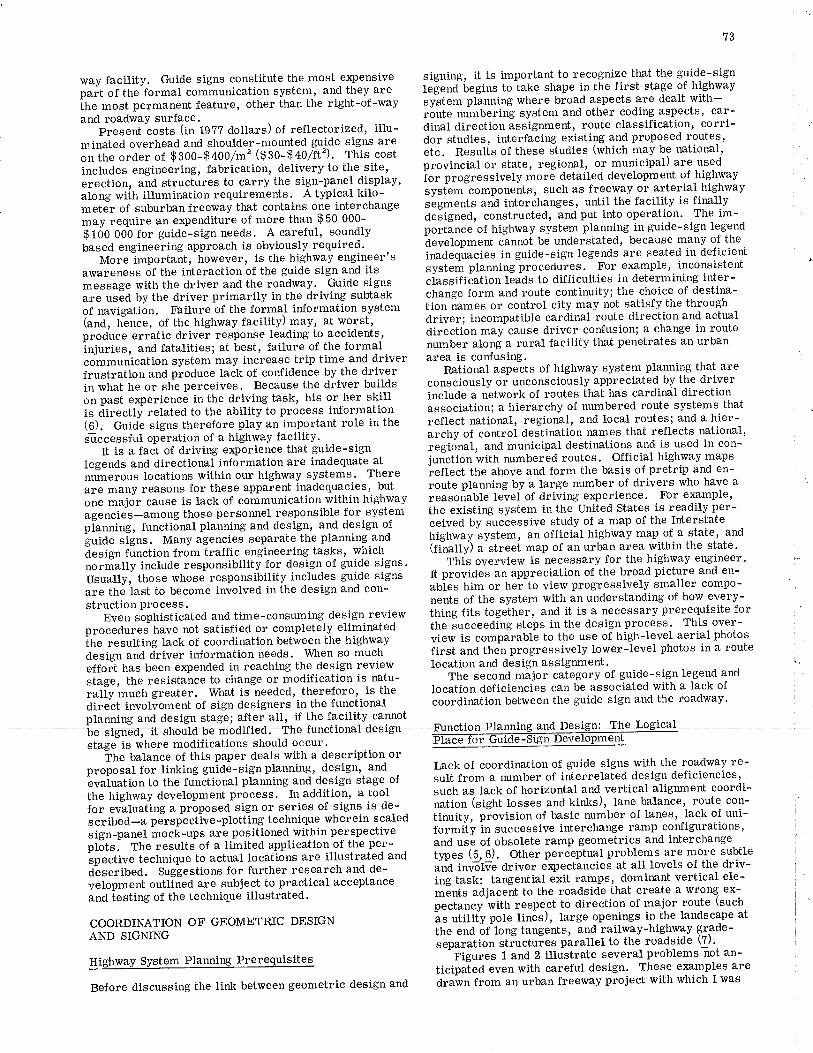
way facility. Guide signs constitute the most expensivepa"t of the formal communication system, and they areihe most permanent feature, other than the right-of-wayand roadwav surface.
Present costs (in 19?? dollars) of reflectorized, illu-minated overhead and shoulder-mounted gu-ide signs areã" lrt" o"a"" of $300-$400/m'z ($so-$ o/rf). This costincludes engineering, fabrication, delivery to the site'erection, and structures to carry the sign-panel display'along with illumination requirements. A typical kilo-meter of suburban freeway that contains one interchangemay require an erpenditure of more than $ 50 000-
$fOO OOb for guide-sign needs. A careful, soundlybased engineering approach is obviously required.
More important, however, is the highway engineer'sawareness of the interaction of the guide sign and itsmessage with the driver and the roadway. Guide signsa"e osed by the driver primarily in the driving subtaskof navigation. FÞilure of the formal information system(and, hãnce, of the highway facility) may, at r,vorst,produce erratic driver response leading to accidents,injuries, and fatalities; at best, failure of the formalcommunication system may increase trip time and driverfrustration and produce lack of confidence by the driverin what he or she perceives. Because the driver buildson past experiencè in the driving task, his or her skillis directly related to the ability to process information(O). Guide signs therefore play an important role in the
successful operation of a highway facility.It is a fact of driving erçerience that guide-sign
legends and directional information are inadequate at
tttme"o.ts locations within our highway systems. Thereare many reasons for these apparent inadequacies, but
one majõr cause is lack of communication within highwayagencies-among those personnel responsible for systemplanning, functiõnal planning and design, and design ofguide signs. Many agencies separate the planning and
ãesign function from traffic engineering tasks, whichnorrially include responsibility for design of guide signs'Usually, those whose responsibility includes guide signsare the last to become involved in the design and con-struction Process.
Even sophisticated and time-consuming design reviewprocedureJ have not satisfied or completely eliminatedihe resulting lack of coordination between the highwaydesign and driver information needs. When so mucheffoit has been e:çended in reaching the design reviewstage, the resistance to change or modification is natu-rafy much greater. What is needed, therefore, is the
direct involvement of sign designers in the functional
?3
signing, it is important to recognize t}:rat the guide-signleãend ùegins to take shape in the first stage of highwaysyitem planning where broad aspects are dealt with-róute numbering system and other coding aspects, car-dinal direction assignment, route classification, corri-dor studies, interfacing existing and proposed routes,etc. Resulis of these studies (which may be national,provincial or state, regional, or municipal).are used
io" p"og"e.tively more detailed development of highway
system-components, such as freeway or arterial highway
sägments and interchanges, until the facility is finallydeãigned, constructed, and put into operation. The im-portánce'of highway system planning in guide-sign legend
ãevelopment cannot be understated, because many of the
inadequacies in guide-sign legends are seated in deficientsystem planning procedures. For erømple, inconsistentciassifiõation leads to difficulties in determining inter-change form and route continuity; the choice of destina-tion names or control city may not satisfy the throughdriver; incompatible cardinal route direction and actualdirectíon may cause driver confusion; a change in routenumber along a rural facility that penetrates an urbanarea is confusing.
Rational aspects of highway system planning that areconsciously or unconsciously appreciated by the driverinclude a network of routes that has cardinal directionassociation; a hierarchy of numbered route systems thatreflect national' regional, and local routes; and a hier-archy of control destination names that reflects national,regional, and municipal destinations and is used in con-junction with numbered routes. Official highway maps
ieflect the above and form the basis of pretrip and en-
route planning by a large number of drivers who have a
reasoiable levei of driving experience. For example,the existing system in the United States is readily per-ceived by successive study of a map of the Interstatehighway system' an official highway map of a state, and
Ginally) a street map of an urban area within the state 'This overview is necessary for the highway engineer'
It provides an appreciation of the broad picture and en-
ables him or her to view progressively smaller compo-
nents of the system with an understanding of how every-thing fits together, and it is a necessary prerequisite forthe succeeding steps in the design process. This over-view is comparable to the use of high-level aerial photos
first and then progressÍvely lower-level photos in a routelocation and design assignment.
The second major category of guide-sign legend and
location deficiencies can be associated with a lack ofcoordination between the guide sign and the roadway'
planning and design stage; after all, if the facility-cannotæR"-"ouro ¡e mo¿:lred;-ihsrunctional design Funetjgn Plar,rlinäandJel
stageis where modifications should occur. Prace rorihe balattce of this paper deals with a description or
proposal for linking guiaô-sien planning, a"tignl ana ral\ot coordination of guide signs with the roadway re-
evaluation to the functional planning ano aesigi-Ëtagã of sult, from a number of interrelated design deficiencies,
the highway development process. In aaaitioü, ã tõoi such as lack of horizontal and vertical alignment coordi-
for evaluating a proposed sign or series or rignr i" ¿"- natio.n (sight losses and kinks), lanetalance,- route- con-
scribed-a perspective-plotting technique wneîÀin scaled tinuity, provision of basic number of lanes, lack of uni-
sign-panel mock-ups are positioned within p"""pã.Ii"" rormití in successive interchange ramp configurations'
plots. The results of ã timite¿ application-oitfti p."- and usè of obsolete ramp geometrics and interchange
spective technique to actual locatiôns are ittustràñO anO types (5,6)' Other perceptual problems are more subtle
described. Suggestions for further research and de- anA invotve driver e4)ectancies at all levels of the driv-
velopment ouilined are subject to practical acceptance ing task: tangential exit ramps, dominant vertical ele-
and testing of the technique illustrated. ments adjacent to the roadside that create a wrong ex-pectarrcy ïith respect to direction of major route (such
COORDINATION OF GEOMETRIC DESIGN ãs utilityp,ole linès), .large openings in the landscape at
AND SIGNING the end óf tong tangents' and railwav-highway grade-
."p""áiiott stiuctuies pâra[el to the, roadsid" 9)'.Highway system planning prerequisites Fígures 1 and 2 illustrate several problems not an-
ticipated even with careful design' These e>rarnples are
Before discussing the link between geometrÍc design and drawn from an urban freeway project with which I was
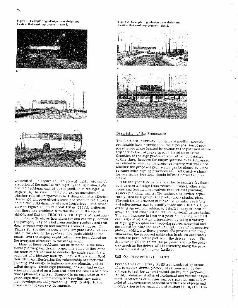
74
Figure 1. Example of guide.sign panel design andlocation that need improvement: s¡te 1.
Figure 2, Example of guide-sign panel design andlocation that need improvement: site 2.
Description of the Framework
The functional drawings, in plan and profile, providereasonable base drawings for the superposition of pro-posed guide signs located by station in the plan and shownadjacent to the roadways in each direction of travel.Graphics of the sign panels should not be too detailedat this time, because the major question to be addressedis related to whether the proposed signing will work andwhether the proposed geometrics can be signed by usingrecommended signing practices (8). Alternative signs
-for particular locations should be-considered and dis-played.
associated. In Figure la, the view at night, note the ob_struction of the panel at far right by the light standardsand the problems caused by the position of the lighting.Figure lb, the view in daylight, raises questions ofwhether relocation upstream or a diagrammatic alterna-tive would improve effectiveness and whether the arrowson the two right-hand panels are ineffective. The closerview in Figure 1c, from about 100 m (ggO ft), indicates
The designer then is in a position to acquire feedbackby means of a design team review, in which other engi-neers and technicians involved in functional planning,system planning, and traffic engineering review sepa-rately, and as a group, the preliminary signing plan.Through the interaction of these individuals, revisionsand adjustments can be readily made and a basic signingdrawing agreed on, subject to detailed study of locaiion,that there are problems with the desiEn of the
ful. Figure 2a shows how signs for one roadway, acrosstlte parapet, may be read from another roadway and thatdown arrows may be meaningless around a curve, InFigure 2b, the down arrow on the left panel does not re-late to the view of the roadway, the route shield is toosmall, and the display might better have been placed onthe overpass structure in the background.
Many of these problems can be detected in the func-tÍonal planning and design stage; this stage is thereforethe most effective time to develop the guide signs for a-s-egmgnt
of a highway facility. Figure 3 is a simplifiedflow diagram illustrating the relationship of functlonalplanning and design to highway system planning and de-tailed design. Guide sign planning, design, and evalu-ation are depicted as a loop that uses the results of func-tional planning studies. Figure 4 is an epansion of theguide-sign task, commencing with preliminary guide-sign development and proceeding, step by step, to thepreparation of contract documents.
erds and that the THRU TRAFFIC sign is not meaning_ The sign designer is then in a position to study in detaileach sign panel and its alternatives by using a varietyof signing principles and procedures recommended anddescribed by King and Lunenfetd (9). Use of perspectiveplots in addition to these proceduiõs provides the thirddimension; the proposed guide sign is shown accuratelywithin the perspective plot from the driverrs eye. Thédesigner is able to relate the proposed sign to the road-way much as the driver will in traveling along the pro-posed (or existing) highway facility.
USE OF PERSPECTIVE PLOTS
Perspectives of highway facilities, produced by meansof a computer-driven plotter, have been used by de-signers to test for general visual quality of a proposedfacility, detailed studies of horizontal and verticál align-ment, aesthetics of bridges and overpasses, and safety-related improvements associated with fixed objects anàmodification to the roadside and median (4, 10, 11). Ex-
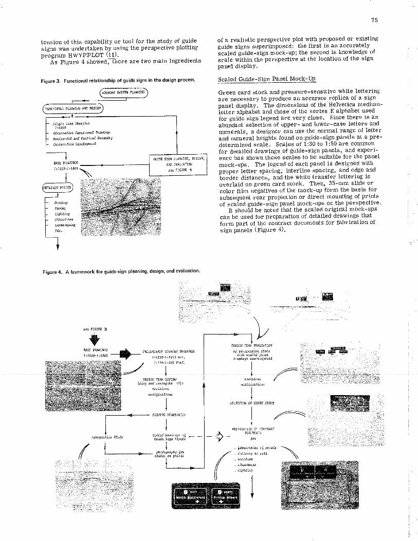
tension of this capability or tool for the study of guide
signs was undertaken by using the perspective plottingp"õg"am HWYPPLOT (11).-
Ãs Figure 4 showedlhere are two main lngredients
75
of a realistic perspective plot with proposed or existingguide signs superimposed: the first is an accuratelyãcated guiae-sign mock-up; the second is knowledge ofscale within the perspective at the location of the signpanel display.
Scaled Guide-Sign Panel Mock-UP
Green card stock and pressure-sensitive white letteringare necessary to produce an accurate replica of a signpanel display. The dimensions of the Helvetica medium-ietter aþhabet and those of the series E alphabet usedfor guide sign legend are very close. Since there is an
abuñdant selection of upper- and lower-case letters and
numerals, a designer can use the normal range of letterand numeral heights found on guide-sign panels at a pre-determined scale. Scales of 1:30 to 1:50 are commonfor detailed drawings of guide-sign panels, and experi-ence has shown these scales to be suitable for the panel
mock-ups. the legend of each panel is designed withproper letter spacing, interline spacing, and edge and-¡o"ãe"
distances, and the white transfer lettering isoverlaid on green card stock. Then, 35-mm slide orcolor film negatives of the mock-up form the basis forsubsequent rear proiection or direct mounting of printsof scaied guide-sign panel mock-ups on the -perspective'
It should be noted that the scaled original mock-upscan be used for preparation of detailed drawings thatform part of the contract documents for fabrication of
sign panels (Figure 4).
siqte Line shQ.tchü1ú800
,'ll.ùnaùiv e t uncf'íanaL ,wingtHmjzonføL Md vüiícol CwelÌqcÃo ¿ áeol it t 0 e! øLoPQltt
Figure 4. A framework for guide-sign planning, design, and evaluat¡on'
1 t1200-1.2400
Ih¡rtttto otslcu I
lo*^"I Pav.íng
L ,a¡*,^L saurn^*L"r¡^"oo,*I E".
t
EE.'' fl
---s¿ìil+=:
Figure 3. Functional relationship of guide signs in the design process'
G{IltE SIC,,I PtÁNl'Jl¡lG, tESlGN,
^u0 EvALU^ll0N
Ãøø FIA/RE +
¿¿¿ F¡GURE 3
,ESTO,,I TEA{ ÊV ALUATT ON
o I pwp¿ct iuø plotÁwí.th ócalQ.d pMel
d,;'p!au' óupeûnpoaed
I
I
LøviÁiotÁ
nod'L(ícaLi.aøII
I
Ert lF
MEPÁRÂTIOI' dF COI{ÎRÁCÍ
-N ,ocuMEl{rs
Y óotL
sErEcfro¡/ 0F cuttE s¡GÂrs
, labLica.lLoÍ oó pare|Å
. de.LLvuA 10 Äi.tø
. uee.tLon
, áþua.îuü. UghrínS
/:
i,:, :,Y,iffi -Ð- n"' l',X', :',:,1' of :y'
*'
,ESIG¡,I fEÁq REUÍEI'lKit4 uÅ Lunøtte,ll, I9)l
Lev¡Áíoünod'i(,batinø
Püpe..tLv¿ PbîÁ
I4,:mnffWsciLQl. O@iigô ol
Guid¿ si4n PMZIÁI
I
\
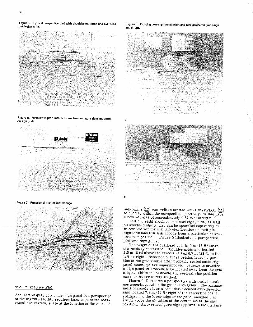
76
Figure 5. Typical perspective plot with shoulder-mounted and overheadguide-sign grids.
-t
l{"{
Il,,rrr,r,rr]
. LOCAT¡ON OF SIGN STRUCTURB. e9Z + 7O. OASeRVER POSITIONT egt , 70
ÂSADINC D¡STANCET 600 FT.CROêSLINE SPACINGT tOO pT.SICN PANEL cR¡o sPAciNc¡ e FT.
Figure 6. Perspective plot with exit.direction and gore signs mountedon sign grids.
LI)C.aTI(JN OF SIGN STRUCTURÊI agz .OES:BVER POSIIION¡ e69 r 70ÂSADII{G OISTANC€. 600 FT.CRUSSLINE SPACINGT tCJ Fl.SICN FAI{81 CnlD SPACING¡ ¿ Fl.
Figure 7. Functional plan of ¡nterchange.
<i'li!¡rar::
Figure 8. Ex¡st¡ng gore sign ¡nstallation and rear.projected guide-signmock-ups,
':)h I ::rì¡l Slntl(.lUÃE¡i.;i ,:1 .(j\t¡ ¿:lu '.-, : -..,,:i:¡ 5.ì3 ¡'.i¡¡1 , ;.- 'i.,r i ì,-, ii'...\l.
,.. -; ^1..l¡.i ! .. -
¡0:
70
The Perspective Plot
Accurate display of a guide-sign panel in a perspectiveof the highway facility requires knowledge of the hori_zontal and vertical scale at the location of the sign. A
subroutine (12) was written for use with HWyppLOT (11)to create, wllhin the perspective, plotted grids that haîèa nominal size of approximately 0.6? m (exactly 2 ft).
Left and right shoulder-mounted sign grids, as wellas overheâ drign€xjdsr €an$e speeif ied separatel¡orin combination for a single sign location or multipiesign Iocations that will appear from a particular ãriver_observer position. Figure 5 illustrates a perspectiveplot
',vith sign grids.The origin of the overhead grid is 5 m (16 ft) above
the roadway centerline. Shoulder grids are located2.5 m (B ft) above the centerline and 6.? m (22 ft) to t¡eleft or right. Selection of these origins 1eaves a por_tion of the grid visible after properly scaled guide_signpanel mock-ups are superimposed, because in practiõea sign panel will normally be located away from the gridorigin. Shifts in horizontal and vertical sign positioncan then be accurately studied.
Figure 6 illustrates a perspective with scaled mock_ups superimposed on the guide-sign grids. The arrange_ment of panels shows a shoulder-mounted exit-directionsign located 7.3 m Q4 ft) right of the centerline of theroadway and the lower edge of the panel mounted B m(10 ft) above the elevation of the centerline at the signposition. An overhead gore sign appears in the distãnce
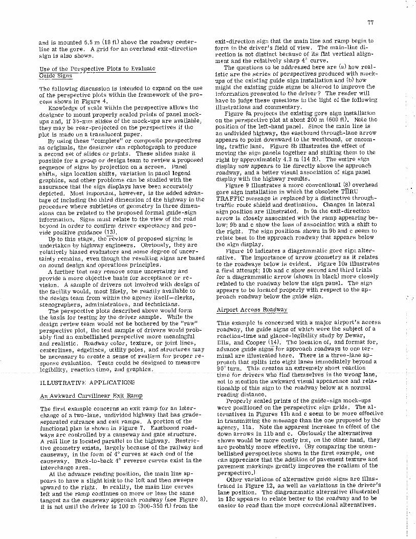
77
and is mounted 5.5 m (18 tt) above the roadway center- exit-direction sign that the main line and ramp begin toline at the gore. A grid for an overhead exit-direction form in the driver?s field of view. the main-line di-sign is also shown, rection is not distinct because of its flat vertical align-
ment and the relatively sharp 4o curve.Use of the Perspective Plots to Evaluateffi
The questions to be addressed here are (a) how real-istic are the series of perspectives produced with mock-ups of the existing guide sign installation and (b) trow
The following discussion is intended to erçand on the use might the existing guide signs be altered to improve the
of the perspective plots within the framework of the pro - information presented to the driver ? The reader willces" s-hown in Figure 4. have to judge these questions in the light of the following
Knowledge of scale within the perspective allows the illustrations and commentary.designer to mount properly scaled prints of panel mock- Figure Ba projects the existing-go"e,liqn-.in"ta_llationups ãnd, if Bb-mm-sliães óf the moìk-ops aie available, oû the perspective plot at aþout 200 m (600 ft). Note the
ttrey may be rear-projected on the perspectives if the position of the left-hand panel. Since the main line isplot is made on a translucent paper. an undivided highway, the eastbound through-Iane arrow
By using these "complete" or composite perspectives appears to point downward to the westbound, or oncom-as oiiginali, the designìr can rephotograph to produce ing, traffic lane. Figure Bb illustrates the effect ofa second set of slides or prints. These slides make it moving the sign panels together and shifting them to thepossible for a group or design team to review a proposed righi by approximately 4.3 m (f¿ tt). The entire signieqoence of signs by projection on a screen. Panel display now appears to lie directly above the approachshúts, sign loõation shifis, variation in panel legend roadrüay, and a better visual association of sign panelgraphics, and other problems can be studied with the display with the highway results .
assurance that the sign displays have been """o"*tÀty
-figure I illustrates a more conventional (8) overhead
depicted. Most important,- however, is the added adïan- gore sign installation in which the obsolete TERUtafe of including thã third dimension of the highway in the IRAFFIC message is replaced by a distinctive through-präcedure wherã subtleties of geometry in three dímen- traffic route shield and destination. Changes in lateralsions can be related to the proposed formal guide-sign sign position are illustrated. In 9a the exit-directioninformation. Signs must retatè to the view of the road arrow is closely associated with the ramp appearing be-beyond in order to confirm driver expectancy and pro- low; 9b and c show the loss of association with a shift to
viãe positive guidance (13). the right. The sign positions shown in 9b and c seem to
Up to ttris Átage, the-review of proposed signing is relate best to the approach roadway that appears below
undertaken by highway engineers. Obviously, they are the sign display.relatively biásed evaluators and some degree of uncer- Figure 10 indicates a diagrammatic gore sign alter-tainty remains, even though the resulting signs are based native. The importance of arrow geometry as it relateson sóund design and operJtions principles. to the roadways below is evident. Figure 10a illustrates
A further test may remove some uncertainty and a first attempt; 10b and c show second and third trialsprovide a more objective basis for acceptance
"o" ""-
for a diagrammatic arrow (shown in black) more closelyui.iotr. A sampte-of drivers not involved with design of related to the roadway below the signpanel. The signthe facility wo.tld, most likely, be readily available to appears to be located properly with respect to the ap-the design team from within the agency itself-clerks, proach roadway below the guide sign.stenographers, administrators, and teehnicians.
Thè nersoective plots described above would form Airport Access Roadwaythe basis for testing by the driver sample. While thedesign review team would not be bothered by the "raw't this example is concerned with a major airportrs accessperspective plot, the test sample of drivers would prob- roadway, the guide signs of which were the subject of aä¡tylinA an ãmbellished perspective more meaningful reaction-time and.glance-legibility study by Dewar,and realistic. Roadway ôo1or, texture, or joint lines, Ells, and Cooper (1Ð, the location of, and format for,centerlines, edgelines, utility poles, and structures may advance guide signs for approach roadways to one ter-be necessary to create a sense of realism for proper re- minal are illustrated here. There is a three-lane ap-sponse evatúation. Tests could be designed to measure proach that splits into eight lanes immediately beyond alÀøihilif v, rea.etion time. and Eranhics. 90o turn. This creates an extremely short reactiontegibility. reaction time, and graphics. 90o turn. This creates an extremely short reaction
ffiinilt@lane,not to mention the awkward visual appearance and rela-tionship of this sign to the roadway below at a normalreading distance.
Properly scaled prints of the guide-sign mock-upswere positioned on the perspective sign grids. The al-ternatives in Figures 11b and c seem to be more effectivein transmitting the message than the one proposed by theagency, 11a. Note the apparent increase in effect of thedown arrows in l1b and c. Obviously the altern¿tivesshown would be more costly but, on the other hand, theyare probably more effective. (By comparing the unem-bellished perspectives shown in the first e)<a.mple, onecan appreciate that the addition of pavement texture andpavement markÍngs greatty improves the realism of theperspective.)
Other variations of alternative guide signs are illus-trated in Figure 12, as well as variations in the drivertslane position. The diagrammatic alternative illustratedin 12c appears to relate better to the roadway and to beeasier to read than the more conventional alternatives'
ILLUSTRATTVE APPLICATIONS
An Awkward Curvilinear Exít RamP
The first exâmple concerns an exit ramp for an inter-change of a two-lane, undivided highway that has grade-separated entrance and exit ramps. A portion of thefunctional plan is shown in Figure 7, Eastbound road-r,vays are controlled by a causeway and gate structure.A rail line is located parallel to the highway. Restrie-tive geometry exists, largely because of the railway andcauseway, in the form of 4o curves at each end of thecauseway, Elack-to-back 4o reverse curves exist in theinterchange area,
At the advance reading position, the main line ap-pears to have a slight kink to the left and then sweepsupward to the right. In reality, the main line curvesleft and the ramp continues on more or less the sametangent as the cáuseway approach roadway (see Figure B).It is not until the driver is 100 m (300-350 ft) from the
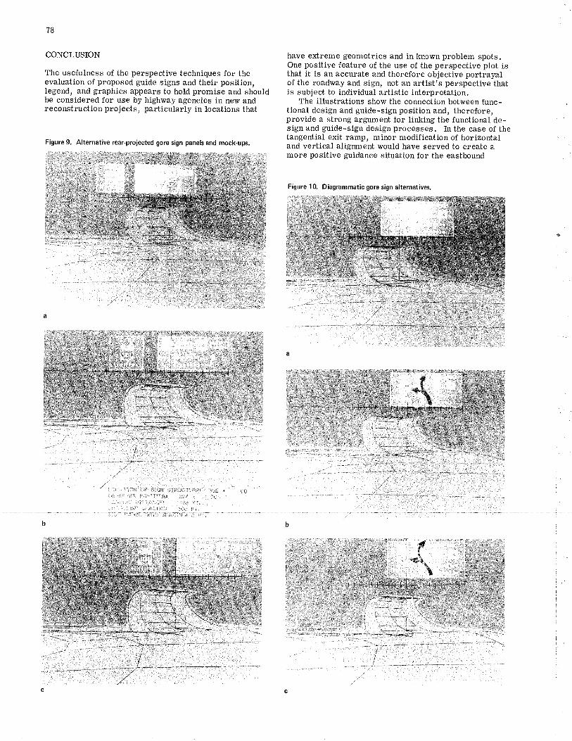
?8
CONCLUSION
The usefulness of the perspective techniques for theevaluation of proposed guide signs and their position,legend, and graphics appears to hold promise and shouldbe considered for use by highway agencies in new andreconstruction projects, particularly in locations that
have extreme geometrics and in known problem spots.One positive feature of the use of the perspective ptot isthat it is an accurate and therefore objective portrayalof the roadway and sign, not an arttst?s perspective thatis subject to individual artistic interpretation.
The illustrations show the connection between fune-tional design and guide-sign position and, therefore,provide a strong argument for linking the functional de-sign and guide-sign design processes. In the case of thetangential exit ramp, minor modification of horizontaland vertical alignment would have served to create amore positive guidance situation for the eastbound
Figure 9. Alternative rear.projected gore sign panels and mock.upa,
Figure 1 0. D iagrammatic gore sign alternatives.
30a + 00oo
LOcÁllof OF StcN C¡RUC-rURB|ù8Þf;RvgR POS¡rDil¡ ?97 .!ì3.1('r rG D¡SIANCE. 439 FT.cRi,'.:;tNq sPAÈtNo¡ l0o Fl.
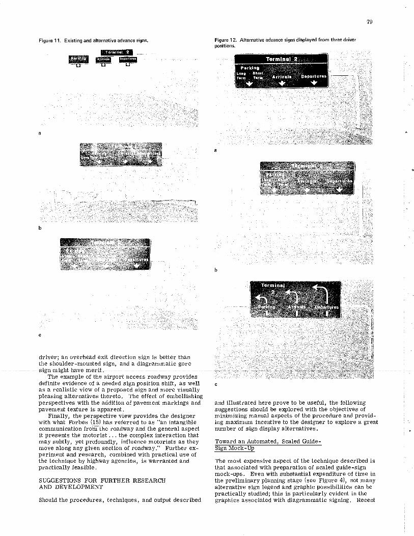
19
Figure 1 1. Existing and alternative advance signs. Figure 1 2. Alternative advance signs d isplayed f rom three driverpositions.
Tormlnal 2- ,..Pr.rklng '
Lor¡ t¡crt Attlvala Depailuresf..t ' lar!.:J W v
_, :,,-l--::---------t
c
driver; an overhead exit direction sign is better thanthe shoulder-mounted sign, and a diagrammatic goresign rnighË have merit. , rt;-:'
The example of the airport access roadway provides : .*ggdefinite evidence of a needed sign position shift, as wellas a realistic vie\,v of a proposed sign and more visuallypleasing alternatives ttrereto. The effect of embellishingperspectives with the addition of pavement markings andpavement texture is apparent.
Finally, the perspective view provides the designerwith what Forbes (tS) tras referred to as "an intangiblecommunication froñã-the roadì,vay and the general aspectit presents the motorist . , . the complex interaction thatmay subtly, yet profoundly, influence motorists as theymove along any given section of roadway," Ftrrther ex-periment and research, combined with practical use ofthe technique by highway agencies, is warranted andpractically feasible.
SUC¡GESTIONS FOR FURTHER RESEARCHAND DEVELOPMENT
Should the procedures, techniques, and output described
c
and illustrated here prove to be useful, the followingsuggestions should be explored with the objectives ofminimizing manual aspects of the procedure and provid-ing maximum incentive to the designer to explore a greatnumber of sign display alternatives.
The most extrlensive aspect of the technique described isthat associated with preparation of scaled guide-signmock-ups. Even with substantial expenditure of time inthe preliminary planning stage (see Figure 4), not manyalternative sign legend and graphic possibilities can bepractically studied; this is particularly evident in thegraphics associated with diagrammatic signing. Recent
Term ¡ nal2<ì
Parking
II
D6partures
I
Toward an Automated. Scaled Guide-
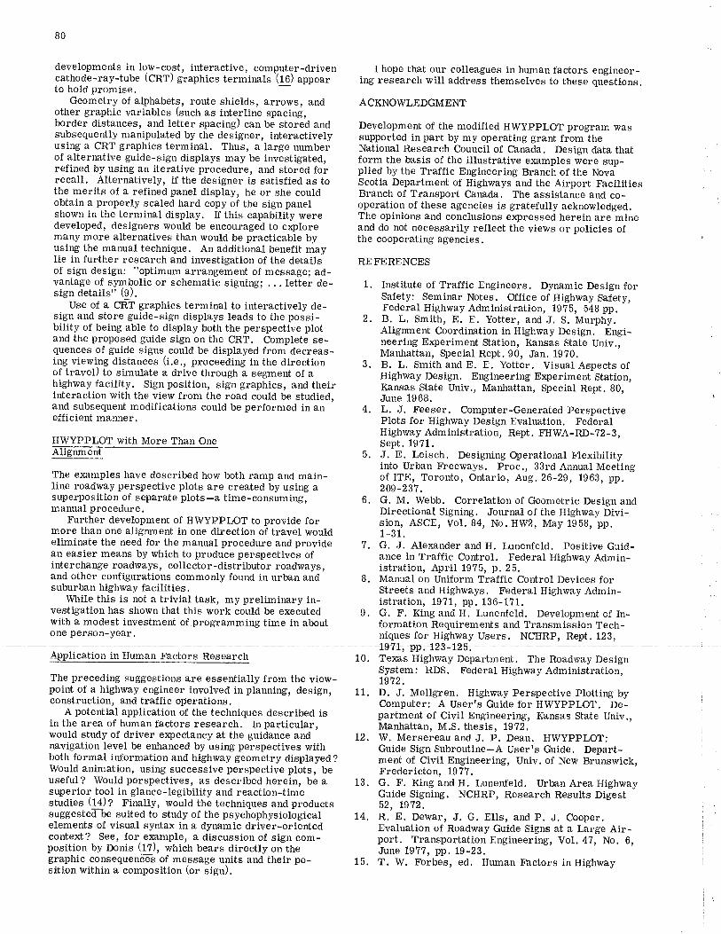
80
developments in low-cost, interactive, computer-drivencathode-ray-tu¡e (Cnf) graphics terminals (16) appearto hold promise.
Geometry of alphabets, route shields, arrotvs, andother graphic variables (such as interline spacing,border distances, and letter spacing) can be stored andsubsequently manipulated by the designer, interactivelyusing a CRT graphics terminal. Thus, a large numberof alternative guide-sign displays may be investigated,refined by using an iterative procedure, and stored forrecall. Alternatively, if the designer is satisfied as tothe merits of a refined panel display, he or she couldobtain a properly scaled hard copy of the sign panelshown in the terminal display. If this capability weredeveloped, designers would be encouraged to e>eloremany more alternatives than would be practicable byusing the manual technique. An additional benefit maylie in further research and investigation of the detailsof sign design: ltoptimum arrangement of message; ad-vantage of sj¡mbolic or schematic signing; . . , letter de-sign details" (9).
Use of a CRA graphics terminal to interactively de-sign and store guide-sign displays leads to the possi-bility of being able to display both the perspective plotand the proposed guide sign on the CRT. Complete se-quences of guide signs.could be displayed from decreas-ing viewing distances (i.e., proceeding in the directionof travel) to simulate a drivè through ã segment of ahighway facility. Sign position, sign graphics, and theirinteraction with the view from the road could be studied,and subsequent modifications could be performed in anefficient manner.
HWYPPLOI with More Than OneffiThe enamples have described how both ramp and main-line roadway perspective plots are created by using asuperpos ition of separate plots -a time - co nsuming,manual procedure.
F\rrther development of HWYPPLOT to provide formore than one alignment in one direction of travel wouldeliminate the need for the manual procedure and providean easier means by which to produce perspectives ofinterchange roadways, collector-distributor roadways,and other configurations commonly found in urban andsuburban highway facilities.
While this is not a trivial task, my preliminary in-vestigation has shown that this work could be executedwith a modest investment of.programming time in aboutone person-year.
I hope that our colleagues in human factors engineer-ing research will address themselves to these questions.
ACKNOWLEDGMENT
Development of the modified HWyppLOT program wassupported in part by my operating grant from theNational Research Council of Canada. Design data thatform the basis of the illustrative er<amples were sup-plied by the Traffic Engineering Branch of the NovaScotia Department of Highways and the Airport FbcilitiesBranch of Transport Cbnada. The assistance and co-operation of these agencies is gratefulty acknowledged.The opinions and conclusions expressed herein are mineand do not necessarily reflect the views or policies ofthe cooperating agencies.
REFERENCES
1. Institute of Traffic Engineers. Dynamic Design forSafety: Seminar Notes. Office of Highway Safety,Federal Highway Administration, 1975, 548 pp.
2. B. L. Smith, E. E. Yotter, and J. S. Murphy.Alignment Coordination in Highway Design. Engi-neering E:iqleriment Station, Kansas State Univ.,Manhattan, Special Rept.90, Jan. 1970.
3. B. L. Smith and E. E. Yotter. Visual Aspects ofHighway Design. Engineering E4reriment Station,Kansas State Univ., Manhattan, Special Rept. 80,June 1968.
4. L. J. Feeser. Computer-Generated PerspectivePlots for Highway Design Evaluation. FederalHighway Adm inistratio n, Rept. ¡IIWA- RD- ?2 - 3,Sept.1971.J. E. Leisch. Designing Operational Fl.exibilityinto Urban Fïeeways. Proc., 33rd Annual Meetingof ITE, Toronto, Ontario, Aug. 26-29, 1963, pp.209-237.G. M. Webb. Correlation of Geometric Design andDirectional Signing. Journal of the Highway Divi-sion, ASCE, Vol. 84, No. HW2, May 1958, pp.1-31 .
G. J. Ale:<ander and H. Lunenfeld. Positive Guid-ance in Traffic Control. Federal Highway Admin-istration, April 1975, p.25.Manual on Uniform Traffic Control Devices forStreets and Highways. Federal Highway Admin-istration, 1971, pp. 136-171.G. F. King and H. LunenJeld. Development of In-formation Requirements and Transmission lech-niques for Highway Users. NCHRP, Rept. 123,
5.
6.
7.
8.
9.
Application in Human Fbctors Research
the preceding suggestions are essentially from the view-point of a highway engineer involved in planning, design,construction, and traffic oþerations,
A potential application of the techniques described isin the area of human factors research, In particular,would study of driver expectancy at the guidance andnavigation level be enhanced by using perspectives withboth formal inJormation and highway geometry displayed?Would animation, using successive perspective plots, beuseful? Would perspectives, as described herein, be asuperior tool in glance-legibility and reaction-timestudies (1Ðl F'inatty, would thã techniques and productssuggested be suited to study of the psychophysiologicalelements of visual syntax in a dynamic driver-orientedcontext? See, for e:<ample, a discussion of sign com-position by Donis (17), which bears directly on thegraphic consequenciË of message units and their po-sition within a composition (or sign),
Federal Highwayt972.D. J. Mellgren. Highway Perspective Plotting byComputer: A Userrs Guide for HWYPPLOT, De-partment of Civil Engineering, Kansas State Univ.,Manhattan, M.S. thesis, 1972,W. Mersereau and J. P. Dean. HWYPPLOT:Guide Sign Subroutine-A User's Guide. Depart-ment of Civil Engineering, Univ. of New Brunswick,Fredericton,1977.G. F. King and H. Lunenfeld. Urban Area HighwayGuide Signing. NCHRP, Research Results Digest52, 1972.R. E. Dewar, J. G. Ells, and P. J. Cooper.Evaluation of Roadway Guide Signs at a Large Air-port. Transportation Engineering, Yol,47, No. 6,June 1977, pp. 19-23.
10. Te:<as HighwaySystem: RDS.
t Ev.Department. The Roadway Design
Administration,
11.
L2.
13.
L4.
15. T. W. Forbes, ed. Human trhctors in Highway
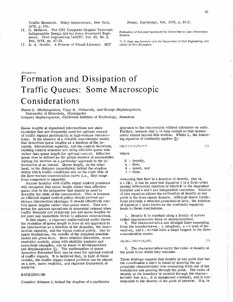
16.
17.
Traffic Research. Wiley-Interscience, New York,1972, p. 130,G. Þllaire. The CRT Computer Graphic Terminal:Indispensible Design Aid for Some Structural Engi-neers. Civil Engineering (AsCn), Vol. 46, No, 2,Feb. 1976, pp.47-53.D. A. Dondis. A Primer of Visual Literacy. MII
Press, Cambridge, MA, 1973, P. 20 ff '
Publication of this paper sponsored by Committee on User lnformatìonSystems.
*J. P. Dean was formerly with the Department of Civil Engineering, Uni-vercity of New Brunswick.
Abridgment
Formation and Dissipation ofTraffic Queues: Some MacroscopicC onsiderationsPanos G. Michalopoulos, Vijay B. Pisharody, and George Steplranopoulos,
University of Minnesota, MinneapolisGre gory Stephanopoulos, California I¡rstitute of Te chnology, Pasadena
Queue lengths at signalized intersections are state approach to the ir¡tersection rvithout entrances or exits.variables tå:at are frequentty used for optimal control Further, assume that L is long enough so that queues
of tra^tfic signals particutarly at high-volume intersec- never extend beyond this section. -Within L, the follow-tions. In the absence of a reliable macroscopic model ing equation of continuity applies ():that describes queue lengths as a function of tfie de-mands, intersection capacity, and the control decisions, (aK/ôt) + (aq/ôx) = 0 (l)existing control schemes are using effective queue sizerather than queue length for optimal control. Effective wherequeue size is defined as the actual number of automobileswaiting for service on a particular approach to the in- K = densityrtersection at an instant. Queue length, on the other { = flow,hand, is the distance immediately behind the stopline x = sPacer andwithin which tra-ffic conditions are on the right side of t = time.the flow-versus-concentration curve (i.e., they rangefrom congested to capacity).
Anyone famitiar with tra-ffic signal control problemswill recognize tù,at queue length rather than effectivequeue size is the parameter that should be used todescribe the state of the intersection. This is becausean efficient signal control policy should prevent up-stream intersection blockage; it should efÏectively con-trol queue tengths rather than queue sizes. This cri-
ion foroptimal-operatisns-i€ €sm€rvhet +€laåred when leadsJsJhese +snelusions,traftic demands are relatively low and queue lengths donot pose any immediate threat to adjacent intersections. 1. Density K is constant along a family of curves
úr this paper, a rigorous mathematical model shows called characteristic lines or characteristics.the evolutibn of queue length in time at any approach to 2. The characteristics are straight lines emanatingthe intersection ãs a funcíion of the demands,
-the inter- from the boundaries-x = L (stopline), x = 0 (end. of thesection capacity, and the signal control policy. Due to section), and t = O-that have a slope tangent to the flow-space limitations, the results of the simplest possible concentration curue:model are given here. More detailed (therefore, morerealistic) models, along with stability analysis and (dx/dt) ='h(k) = (dq/dK) (2)
numerical examples, can be found in Michalopoulousand Stephanopoutos (9. The mathematics of (ueue _ 3. .The characteristics carry the value of density atdynamiðs discussed -here can be used for optimat control the point from which they emanate.of tra-ffic signals. It is believed that, in light of theseresults, ttrJtra-tfic signal control próblemian be placed These findings suggest that density at any point trat has
on a ne*, more rea¡Jtic, and rigõrous framework of the coordinates x and t is found by drawing the ap-analysis. propriate characteristic line emanating from one of the
boundaries and passing through ttre point. The value of
BACKGROUND density at the boundary is carried through the charac-teristic line (i.e., it is maintained constant), and it cor-
Consider distance L behind the stopline of a particular responds to the density of the point of interest. If kr is
Assumíng that flow is a function of density, that is,q = f(K), it ca¡r be seen that Equation 1 is a first-orderpartial differential equation in which K is the dependentvariable and x and t are independent variables. Solutionof this equation allows the estimation of density at anypoint in the time-space domain. Although space limita-tions preclude a detailed presentation here, the solutionof Equation 1 (also known as the continuity equation)
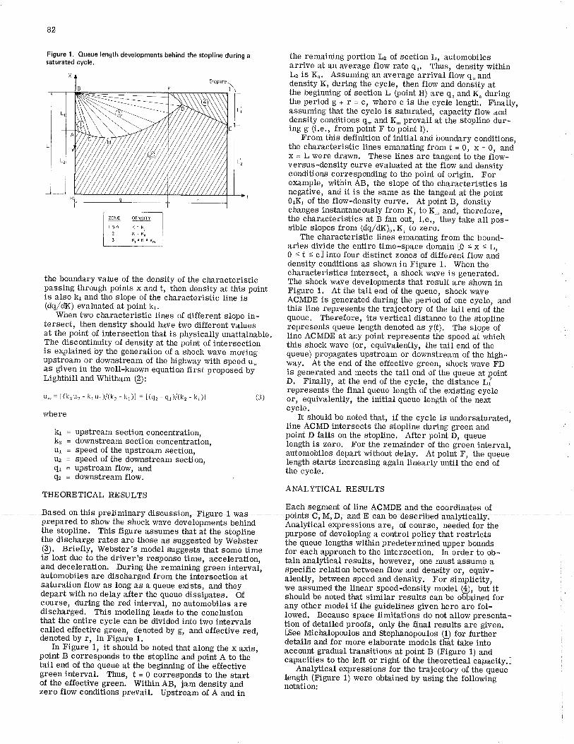
82
Figure 1. Oueue length developments behind the stopline during asaturated cycle.
the boundary value of the density of the characteristicpassing tìrough points x and t, then density at this pointis also kr and the slope of the characteristic line is(dqldlç) evaluated at point kr.
When two characteristic lines of different slope in-tersect, then density should have two different valuesat the point of intersection that is physically unattainable.The discontinuity of density at the point of intersectionis erplained by the generation of a shock wave movingupstream or downstream of the highway with speed u,,as given in tlte well-known equation first proposed byLighthill and Whitåam Q):
u* = [(k, u, - kl u1 )/(k, - kr )] = [(q2 - qr )/(k2 - kr )] (3)
the remaining podion Lz of section L, automobilesarrive at an average flow rate q". Thus, density withinL2 is K". Assuming an average arrival flow q" anddensity K" durlng the cycle, then flow and density atthe begiming of section L þoint H) are qu and Ku durÍngthe period B + r = c, where c is the cycle lengür. Finally,assuming that the cycle is saturated, capacity flow anddensity conditions qm and K- prevail at the stopline dur-ing g (i.e., from point F to point I),
From this definition of initial and boundary conditions,the characteristic lines emanating from t = 0r x = 0, andx = L were drawn. These lines are tangent to the flow-versus-density curve evaluated at the flow and densityconditions corresponding to the point of origin. Forexample, within AB, the slope of the characteristics isnegative, and it is the same as the tangent at the point0rK; of the flow-density curve. At point B, densitychanges instantaneously ftom K, to K_ and, therefore,the characteristics at B fan out, i.e., they take all pos-sible slopes from (dq/dK)., K, to zero.
The charaeteristic lines emanating from the bound-aries divide the entire time-space domain [0 < x < L,0 < t < cl into four distinct zones of difTerent flow anâdensity conditions as shown in Figure 1. When thecharacteristics intersect, a shock wave is generated.The shock wave developments that result are shown inFigure 1. At the tail end of the queue, shock waveACMDE is generated during the period of one cycle, andthis line represents the trajectory of the tait end of thequeue. Therefore, its vertical distance to the stoplinerepresents queue length denoted as y(t). The slope ofline ACMDE at any point represents the speed at whichthis shock wave (or, equivalently, the tail end of thequeue) propagates upstream or downstream of the high-way. At the end of the effective green, shock wave FDis generated and meets the tail end of the queue at pointD. Finally, at the end of t}re cycle, the distance Lírepresents the final queue length of the existing cycleor, equivalently, the initial queue length of the nextcycle.
It should be noted that, if the cycle is undersaturated,line ACMD intersects the stopline during green andpoint D falls on the stopline. After point D, queuelength is zero. For the remainder of the green interval,automobiles depart rvithout delay. At point F, the queuelength starts increasing again linearly until the end ofthe cycle.
ANALYTICAL RESULTS
where
kr=kz=llr =tlz =
Qr=qr=
THEORETICAL RESULTS
upstream section concentration,downstream section concentration,speed of the upstream section,speed of the downstream section,upstream flow, anddownstream flow.
RasedonrhispreriminaÊy¡iseussion, Figuæ 1-w"* jå'j'ii#, f#å+##-#åi,ïäi91"*W"Jr#prepared to show the shock wave developments behind Anat¡icâl é4pressions are, of course, neeåed for tt¡ethe stopline. This figure assumes that at the s_topline pu"pä"u of developing a co¡itrol policy'that restrictsthe discharge rates are those as suggested by Webster in" qu"u" lengths within predetermineO upper boundsfÐ: Briefly, Jilel¡sterls model suggests ttrat some time io" .iacrr apprãach to thelntersection. In order to ob-is lost due to the driver's response.time, acceleration, |¿in analytiõal results, however, one must assume aand deceleration. During the remaining greerr.interval, specific relation betwéen flow arid density or, equiv_automobiles are discharged from the intersection at aientty, between speed and density. noi siápUcity,saturation flow as long as a queue exists, and they we asåumed the linear speed-density model (4), but itdepart with no delay after the queue dissipates. Of sfrouU be noted that similar ""À"iti".* ¡ã-oìídi"J to"gourse, during the red interval, no automobiles^are any other model if the guidelines given here are fol_discharged. This modeling leads to tåe conclusion - lowed. Because space limitations- do not allow presenta_that the entÍre cycle can be divided into two intervals tion oi detailed prõofs, only the final results a"ä giv"rr.called effective green, denoted by g, and effective red, ßã" Ui"fr"fopouto" anâ $eihanopoulos e for furítrer¿"tlot4 by r,.in,Figure 1' details and for more elaborate models that take intoIn Figure 1, it should be noted that along the.x axis,
"ããä"rt gradual transitions at point B (Figure 1) andpoÍnt B conesponds to the stopline and point A to. tIe ;p;;ities to the left or right of the theoretical capacity.Jtail end of the queue at tlre beginning of the effective. -î*fyti"rl
e4pressions for the trajectory of the queuegreen interval. Thus, t = 0 corresponds to the start tengttr lirigu"e fj *"r" oùtained by using the followingof tle-effective green. Within AB, jam density and ;;d;i;",zero flow conditions prevail. Upstream of A and in
83
V(0) = Lr = initial queue length at t = 0ry(c) = Lí = final queue length att = cty(t) = queue length at any time point t,
B = effective green interval,r = effective red interval,c = B+r=cyclelength,
9.,n = minimum green time required forundersaturation,
Xrj = eQuation of anY line IJ,ur = free-flow speed of the approach under
consideration,k, = jam density of the approach under
consideration,Q,, k u = arrival flow and density conditions,
xi,t¡,Y¡ = coordinates ofPointi, andy¡ = eQlation of line IJ with respect to tlte y
axis (Figure 1).
Thus, the following analytical e4pressions can beobtained by following the guidelines that are offered inMichalopoulos and Stephanopoulos Q:
where
b = (k"u¡c/k¡) - [kiuig/4(k¡ - k")] (22)
If c and g are given, b is constant, i.e., it is independentof the initial queue Lr. Thus, Equation 22 can be gen-eralized for any cycle N and rewritten as
L¡11=L¡lb (23)
where Lu and LN*r are the queues at the beginning ofcycle N and N+1. Clearly, a steady state exists ifLn = LN*r or if Ln = Lr'r + b, i.e., if b = 0. Therefore,for steady state
(k"u¡c/k¡) - [\urg/4(k, - k,)l = 0 (24)
and to solve lor gfc
elc=lk¡el4(k:-k,)l =tr Q5)
Since À is positive, it is easily seen that if g,/c < À, thequeue length at the end of the cycle will be growing foras long as this situation persists. Otherwise, if b < 0or, equivalently, g/c > À, the queue at the end of thecycle will decrease. It should be noted that Equations23 and 25 ate meaningful for saturated cycles, i.e., forgreen times less than the ones given by Equation 19.
Otherwise, Ln*r is not related to Lw and it is given fromEquation 20. A final note concerning the stability ofthe steady state is worthy of emphasis. As Equation23 reveals, the steady state is metastable. If b = 0, asmall variation of the demands will change the steadystate to a nearby value tlrat is also metastable. There-fore, the queue length at the begirming of each cycle willchange according to the fluctuating values of b, whichdepend on the demands.
CONCLUSION
The approach taken here to a new and rigorous mathe-matical model and analysis that show the formation anddissipation of traffic queues at signalized intersectionsis macroscopic in nature in the sense th,at automobilesare treated as platoons rather than as single units. Theshock wave analysis is fairly realistic for moderate tohigh demands where the shock waves c¿ln be clearlyrealized. In fact, it is this volume range in which tl¡etraffic signal control problem is more pronounced.The analytical results given here have been used forthe derivation of a real-time control policy that mini-
Xs¡= L-n¡t
Xnc= (L- L,) - [(k,ur/kt)]t
Xc= L- [k;Lri(k¡ - k,)]
tc = [ kj Ll /ui(kr - k")]
Yc= [\Lrl(k: - k,)l
Ycun = [ui + h(k,,)] (t.tc)% - h(k")t
where
h(k,)=urtl -(2k"/kj)ì
tu = [u¡ + h(k,)]'? t,'/4[h(k")1':
yr,¡ = [ui + h(k")1'? t./4[h(k")l
! ¡:¡ = u¡t - ui(tg)%
tn = { (tc)7'+ [u¡(g)/'/u¡ + h(k")] ]'?
vu = ui { tc- [ufh(kÀ)g] iIu¡ + h(k,)1'?
+ [ur - h(k,)] /tur + h(k")l (etc)%l
yur = yo + [u¡k. (t - tD)/kj ]
yt¡= L't = L, + [(k"u¡c)/k;] - [kturgl/4(k; - k")
(4)
(s)
(6)
(7)
(8)
(e)
00)
(11)
(12)
( l3)
( l4)
(1s)
(16)
07)
In an undersaturated cycle, the queue dissipates intime:
s-in = [(yc/tc)+h(k")]'?tcl[h(k,)]'z (19)
This is the minimum green time to dissolve the initialqueue Lr. In such a cycle, the final queue length L{ isindependent of the initial Lr and is given by
yr:=Li=(c_e)(k,uÐ/k¡
QUEUE LENGTH STABILITY
(20)
The analybical relations between the initial and finalqueue developed in the preceding section of this papersan be used for stability analysis. Equation 17 can berewritten as
rsecfl0nconstraints at isolated critical intersections $!). Itis important to note that the tra-ffic queue dynamicsnoted here are valid for isolated intersections at whichthe assumption of constant average flow rates is fairlyrealistic. If traffic arrivals are affected by an upstreamsignal, the analysis becomes more complex. Extensionof ttre basic theory to a system of two or more intersec-tions in succession is not trivial due to the side streetsand sinks or sources between the intersections. Thefact that the ínput flows to the downstream intersectionis a function of the output of the upstream intersectionfor any pair of intersections further complicates theanalysis. 'ffe have also studied the queue dynamicsfor a system of intersections as well as the relatedoptimal traffic signal control problems (!).
It should be recogrrized that the analysis presentedhere does not include all possible combinations of shockwave developments that can occur at signalized inter-sections. Rather, the ones that are most likely tooccur are noted. However, analysis for the cases notLi=Lr+b (21)
Some Research
to Kaufman (Ð, tne former represents an overcasthorizon night sky with the moon and the Latter, anhorizon sky on a very dark day.
Obser:vers adjusted the luminance of a glare sourceto the BCD, which has been the common North Americancriterion for discomfort glare for about 30 years. Thelong instructions say that somewhere between a dimcomfortable light and a bright uncomfortable one is apoint of change or threshold called BCD. They furtherstate that this threshold is neither the one that dis-tinguishes pleasantness and comfort nor the one thatdistinguishes tolerable and intolerable. Rather, atBCD, if the glare source was made just slightly brighter,it would be uncomfortable.
The 97 paid participants in this study-primarilycollege students-adjusted (with replication) the in-
laæßõu¡ce toBCD fOr2S ofthe l2b pos-
B4
discussed can be easily performed by following similarguidelines. A number of other cases and numericalexamples are treated in Michalopoulos and Stepha-nopoulos [).ACKNOWLEDGME¡{I
We would like to acknowledge the support of the NationalScience Foundation and the Program of University Re-search of the U.S. Department of Transportation.
REFERENCES
1. P. G. Michalopoulos and G. Stephanopoulos. De-velopment and Evaluation of Optimal Control Strate-gies for Large-Scale Urban Transportation Networks.Department of Civil and Mineral Engineering, Univ.of Minnesota, Minneapolis, Final Rept., 1gT6.
Abridgntent
Putnam and others (3-Ð ¿ia what might be consideredpilot studies for this experiment by selecting the vari-ables and the range of variation and by running a fewsubjects. The study summarized here is described indetail by Bennett (Q.
Glare source size, position, and background lumi-nance were independent variables; glare source lumi-nance at the borderline between comfort and discomfort(BCD) was the dependent variable.
Glare source size was varied in five equal stepsfrom 10-6 to 10r steradian. At arm's length, thesevary from pinhole size to that of a quarter and wereselected to cover the range of practicable sizes of theluminous parts of roadway luminaires. Source positionvaried in five equal steps from 0o (along the horizon)up to 30o above the line of sight (above the occludingangle of windshield tops). Background luminance wasvaried in five equal steps from 0.0034 cd/m'z 10.OO1footlambert) to 34 cd,/mz (10 footl,amberts). According
Discomfort Glare: A Review of
Corwin A. Bennett, Kansas State University, Manhattan
Extensive research on discom,fort glare as applied toroadways has been done in Europe by De Boer (Ð atrdHopkinson Q. However, discomfort glare reseãrch inthe United States, as has most lighting research, hasfocused on interior applications. In the past few years,discomfort glare research conducted at Kansas StateUniversity under the sponsorship of the IlluminatingEngineering Research Institute has been aimed pri-marily at fixed-roadway Iighting. Thís paper surveysthis research and briefly discusses its applications.
SINGLE-SOURCE STUDY
An initial major study was conducted with a single glaresource,
2. M. H. Lighthill and G. B. Whitham. On KinematicWaves: þrt,2, A Theory of Traffic Flow on LongCrowded Roads. Proc., Royal Society, London,Series 4229, No. 11?8, 1955, pp. 317-345.
3. F. V. lVebster. Traffic Signal Settings. HerMajesty's Stationery Office, London, Road ResearchLaboratory Paper No. 39, 1958.
4. B. D. Greenshields. A Study of Traffic Capacity.Proc., HRB, Vol. 14, 1934, pp. 448-477.
5. G. Stephanopoulos and P. G. Michalopoulos. ReaITime Control of Critical Intersections Based onQueue Dynamics. Proc., IEEE Conference onDecision and Control, San Diego, 19?8, pp. 1018-L024.
Publication of this paper sponsored by Committee on Traffic FlowTh eory an d Ch aracte ri sti cs.
sible combinations of the three variables in a con-foundeddesign. The observer looked at the pole of a 0.6-m(2-ft) radius hemisphere sitting on edge. By using acombination of a transformer and several neutral densityfilters (to reduce the voltage range and, hence, thelamp color variation), the glare source was set to BCD.
Multiple regression analysis, which involved sometrial and error on transformations of variables, wasperformed. However, this work was largely guided bypreviously published research.
Results and Discussion
The selected multiple-regression model is as follows:
BCD = 200 (LB) 0.3 x eo.osA/S0.6
where
BCD (in ca/r#¡ = borderline between comfort anddiscomfort,
Lu (in cd/m'z) = luminance of the background
85
color, whether glasses are worn, type of occupation,and the sunniness of one's residential community werenot significantly or consistently reÞted to BCD.
Although Fisher and Christie (Q found a relation be- the correlation between BCD and BCA was a nonsignif-tween age and disability glare -sensitivity, no other such icant 0.19, thus discouraging the idea of general per-
tfmull-
\r'= uráur,A (in degrees) = source angle above the line of
sight (r = 0,12), ands (in steradians) = source size (r = -0.41).
Comparisons of the results of this study to those ofPutrøm Q-!), Hopkinson (þr and others show essentialsimilarities but with some differences in empirical con-stants, The BCDs in the Kansas State e4periment tendto be higher than earlier results.
A later ex¡reriment with 24 new observers comparedthe source at 22.f above the line of sight to one at22.fto the right of line of sight for the intermediate size andbackground luminance. No significant difference inBCD was found for these conditions.
Although the relative size of the comelations of theindependent variables with BCD might be thought toindicate their reÞtive importance, it is a function ofthe range of variation included in the experiment. Thus,originally there was an angle as large as 60o. This waseliminated because observers frequently could notachieve BCD at this high angle. However, to the extentthat the ranges of variation are ecologically correct(i.e., they properly simulated the real world), the rela-tive correlations are meaningful.
The coefïicients of determination for the regressionanalysis shorv that more (0.ã4) of the predicted variationin BCD is associated with observers (individual dif-ferences) tllan the three independent variables (0.28).This is based on the inclusion in the multiple regressionanalysis of observers as dummy variables. That is,each observer was called "0" or "1" depending onrvhether he or she was currently in the equation or not(i.e., treated as a measure). The substantial coefficientof determination reflects the fact that there were large,consistent (over erçerimental conditions) individualdifferences in glare sensitivity or BCD. This may alsobe seen in the variation in the multiplier of the regres-sion equation. This had a median of 217 (rounded to200 in the equation), with a range from 0.52 to 8800-aratio of almost 1? 000:1. Wide individual variations inglare sensitivity have been long known to glare re-searchers and are discussed in the next section.
INDIVIDUAL DIFFERE NCE S
and discomfort glare have occurred. In 1972, 162visitors during a Kansas State University open housemade glare adjustments and filled out personal infor-mation forms. In 1974 and 1975, 199 open housevisitors did the same. These were then interrelated.This work is described in more detail by Bennett (fl.
Observers adjusted a2.2 x 10-a steradian (one -degree) incandescent Þmp at 0o with a 5.5-cd/m' (1.6 -footlambert) background luminance to BCD. Significantsmall correlations were fqrnd between BCD and age(-0.31), eye color (0.16), and indoor versus outdooroccupations (0.17). Older observers were more glaresensitive (had lower BCDs), and the empirical rela-tion was found to be
BCD, cd/m2 = 86 000/age, years (2)
Light-eyed observers and those with indoor occupa-tions have lower BCDs (are more sensitive). The sizeof one's residential community, a person's sex or hair
almost always produce discomfort, but the moremoderate conditions that may produce discomfort neednot produce disability. Discomfort may be viewed asa warning reaction that could lead to the avoidance ofdisability-producing conditions or,vorse. Similarly,although discomfort and disability apparently have dif-ferent physiological mechanisms, it makes sense forolder people who are more sensitive to disability to bemore sensitive to discomJort effects. People with moremelanin have darker eyes, and the melanin filters outlight so that ihey are less sensitive to glare.
Lane (1Ð found that people who have recently donemore detailed close work (are visually fatigued) aremore sensitive to discomJort. Thus, one might expectindoor workers to be more sensitive also.
Al1 in all, despite a few significant correlations,this research has been rather unsuccessful in accounting ¡for differences in sensitivity to glare in terms of demo-graphic variables. Consequently, M. M. Babiker ina L911 masterrs thesis done at Kansas State Universitystudied personality and attitude variables.
A Personal Enlightment Test, given after preliminaryscreening, was developed that consisted of 6{ per-sonality, attitude, and demographic items. This testhad items such as, "f am in just as good physical healthas most of my friends" (true or false) and, "In youropinion, can headlight glare be prevented" (yes or no).This test was given in 19?7 to 101 open house visitors.The visitors adjusted to BCD in the hemisphere with a1.?6 x 10⁻⁴ steradian source at 0o with a 34-cd./m2(10-footlambert) background lumina^nce. In addition, theobservers made similar white-noise adjustments to theborderline between comfort and annoyance (BCA).
Stepwise regression analysis to predict BCD re-sulted in a22-ítem questionnaire with an R of 0.81. Thetotal sample was arbitrarily subdivided into halves. Anew nine-item question set based on stepwise regressionof one-half of the observers predicted the other set ofdata with an R of only 0.21 (nonsignificant at 0.05).
Thus, again, the attempt to predict who will besensitive to gÞre has proven elusive. It seemedplausible that personality items (largely anxiety items)and glare attitude items would be useful. Ostberg andothers (Ð did find a significant correlation (0.53) be-tween a-test of neuroticism and glare sensitivity. Also,
APPLICATION TO ROADWAYS
In one sense, the Roadway Lighting Committee of theIlluminating Engineering Society is the customer forthe ongoing research. The Standard Practice producedby this committee has not included discomfort gÞrein its considerations. Although European standards doconsider discomfort glare, U.S. and Canadian engineershave encountered difficulties in tests of these proce-dures. Consequently, North American research isunder way.
The single-source experiment gives some resultsthat should be applicable to roadway lighting. In somecases, however, such as at interchanges, vast arraysof many light sources appear in the field of view. Fora line of lights along the driver's roadway, two coun-teracting effects take place. The near lights are largerbut higher above the line of sight. The far lights aresmaller but closer to the line of sight. Research is
Mounting Height Mounting Height Yat 3-m iateral at 9.1-m Laterar various percentages of observers who would be dis-
86
Table 1. Est¡mated BCDs for roadway lighting for a single source.
BcD (cdlm'? o00s)
Longitudinal BåckgroundDistance Luminance(m) (cdlm')
Distance (m) Distance (m)
not. Generally, most discom-fort problems can beavoided by raising the mounting height. Other analysisis under way to figure out how to cope with skewed dis-
comforted.
REFERENCES
1. J. B. De Boer, ed. Public Lighting. Cleaver-Hume Press (Phillips Technical Library), London,1967.
2. R. G. Hopkinson. Discomfort Glare in LightedStreets. In Transactions of the Illuminating Engi-neering Silciety, Illuminating Society, Londãn,
-
1940, p. 5.3. R, C. Putnam and K. E. Faucett. The Threshold
of Discomfort Glare at Lo',v Adaptation Levels.Illuminating Engineering, Vol. 46, No. 10, 1951,pp.505-511.
4. R. C. Putnam and W. F. Gillmore. DiscomfortGlare at Low Adaptation Levels: Part 2, OfT-AxisSources. Illuminating Engineering, Vol. 53, No.4, 1957, pp.226-232.
5. R. C. Putnam and K. D. Bower. Discomfort Glareat Low Adaptation Levels: Part 3, Multiple Sources.Illuminating Engineering, Vol. 53, 1958, pp. 1?4-184.
6. C. A. Bennett. Discomfort Glare: ParametricStudy of Angularly Small Sources. Journal of theIlluminating Engineering Society, Vol. 7, No. 1,1911, pp.2-L5.
1. J. E. Kaufman, ed. IES Lighting Handbook,5th ed. Illuminating Engineering Society, NewYork, 1972.
8. A. J. Fisher and A. W. Christie. A Note onDisability Glare. Visual Research, 1965, pp. 5,565.
9. C. A. Be¡nett. The Demographic Variables ofDiscomfort Glare. Lighting Design and Applica-tion, Vol. 7, No. 1, 19?7, pp. 22-24,
10. B. C. Lane. Lowering of Functional PhotophobiaThreshold with Daily, Substained Closework Ac-commodation. Paper presented at OptometricAeademy Meeting, Birmingham, AL, Oct. 197?.
11. O. Ostberg, P. T. Stone, and R. A. Bensen.Free Magnitude Estimation of Discomfort GI¿reand Working-Task Difficulty. Goteborg Psycholog-ical Reports, VoI. 5, No. 15, 19?5.
Publication of this paper sponsored by Commíttee on Visibility.
12119.1t2119.1
0.00340.0340.343,4
340.00340.0340.343.4
340.00340.0340.343.4
34
11 74
45 5189 100
180 20017 t734 3869 72
13? 140270 29024 2448 5196 99
190 200380 400
2t3879
160310
2751
1102t0410
2t 21 2441 45 4582 86 93
160 1?0 180330 340 38027 27 3155 55 58
110 110 t20220 220 230450 450 480
Notesr I m= 3.3ft; 1 cd/m2 =0.292footlambert,Empry cells ¡ndicate < 20' cutoff to the top of the w¡ndsh¡eld.
under way to study such multiple-source effects.h the meantime, Merle Keck of Westinghouse and
Ramkumar Viswanathan of Ka¡sas State each didanalyses that related some representative roadway-lighting conditions to those involving a single lightsource. Table 1 shows BCDs estimated from an arialysisbased on the regression equation from the single-sourcee4periment.
It was assumed that a varying visible portion of a0.13-m'z (200-in'z) cobrahead luminaire wás mounted at9.1 m (30 ft), 11 m (35 ft), or 12 m (40 fÐ. The drivertsline of sight was assumed to be 1.2 m (4 ft) above tìeground. The lights were assumed to be either 3 m (10ft) or 9.1 m (30 ft) to the side of the driver's track. TheBCD was exa.mined at21 m (90 ft), 55 m (180 ft), and82 m (270 ft) longitudinally from the light.
fn some cases, the light at closer distances wasabove the occluding windshíeld top. The BCDs may beappraised by observing that Viswanathan and I made afew luminance measurements of roadway lights in ourneighborhood that ranged from 21 000 cd/m' (6000 foot-lamberts) to 86 000 cd/m" ¡25 000 footlamberts) (formercury, high- and low-pressure sodium). If such anactual source luminance was viewed in a position wherea lorver BCD luminance was expected, one might expectat least half the observers to be uncom-fortable. Thus,some analyzed conditions will be problems, some will
Economic Models for Highway andStreet Illumination DesignsRichard rü. Slocum and Daniel R. Prabudy, Research and Development Division,
Ministry of Transportation and Communications, Ontario
A key issue in the field of ¡llumination is energy conservation. At thesame t¡me, the application of economic resources should be optimized.For instancg, to save energy, roadway illumination lamps can be replacedby more efficient lamps that provide the same light for less wattage.However, such energy savings may be oîfset by other cost elements. For
these reasons, deta¡led cost calculations are needed to ensure lighting in-vestment optimizat¡on, The cost-effectiveness of l¡ghting systems can beestablished by the discounted total cost or annual equivalent costmodels described in this report. These economic models allow variouscost items, such as capital outlay, maintenance, and operational and en-
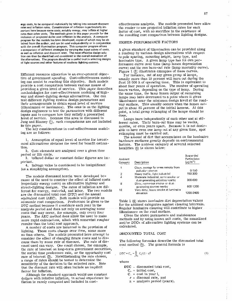
1. Assumption of equar lever of service for invesr- *Ji""i*"#å::3ij"t#li:i:ffi3ii""Ïitlii,1T#lät""ment alternatives obviates the need for benefit estima- factors. The ambiãnt cat-egoiy of several selectedtion' localities ($ is shown below:
2. Cost elements are anaLyzed over a given timeperlod or life cycle. Suspended3. InJlated dollar or constant dollar figures are im- Ambient particulatesportant. - Category Description (pglm3 )
4. Salvage value is considered to be insignificant(as a simprifying assumption).
q tv pç rrlСõ¡uuve¡¡ç i clean, average for areas remote from n_rñnpollution sources 0-150
rhe modets discussed herein were deveroped be- í il,:îi,.jlåü]å;'JilJ lXlillll\oo..o,- 150-300
cause of the need to consider the effect of in-ftated costs dust-generating activities nearby 300-600(especially energy costs) on alternative highway and I Dirty, numerous smoke- or dust-
street-lighting designs. The rates of ir¡fþtion are dif- generating sources nearby 600-1200
ferentfoi"tte-"gy, ñaterial, andlabor. Thetwomodels '16 Verydirty,heavysmokeatluminaire ..^^â¡^ñare the oiscoutrîéä total cosi (DTC) and the aruual elevation 12oo-24oo
equivalent cost (AEC). noth models will provide aneconomic cost còmparison. preference ii given to the !aff9 1 (!)- girows luminaire dirt depreciation values
DTC method because it considers each yeaiin the for the ambient categories against cleaning intervals.eg*bfluminaire-eleaning-willeont+itrute to
costÀ thal may occur, for examfle, only every four illuminance on the road surface.years. The ÁEC meihod Aoes auow ths user io make Given the above parameters and maintenance
more rapid calculations, albeit u¡ith somewhat rougher methods and by using known unit costs, the annualized
results than the total coSt approach. aîd/or DTCs of alternative lighting systems can be
A number of costs are incìrred in the provision of calculated'
ergy costs, to be compared realistically by taking into account discountrates and inflation rates. Consideration of inflation is particularly im-portant here because some costs, notably energy, may inflate at h¡gherrates than other costs. The methods given in this paper provide for theinclusion of prolected dollar cost inflation ¡n the analys¡s. A computerprogram for the models has been developed, copies of which may be ob-ta¡ned from the author, and can be used independently or in conjunctionwith the overall illumination program. This computer program allowsa comparison of d¡fferent strateg¡es by varying the input values of costs,as well as inflation and discount rates. The most effective design solu-tion can then be identif¡ed and considered in the overall evaluation ofthe alternat¡ves. The program should be a useful tool in selecting designsof l¡ght sourc€s and other features of roadway lighting systems.
Efficient resource allocation is an ever-present objec-tive of government spending. Cost-effectiveness model-ing can assist in reaching this objective. Such modelsprovide a cost comparison þetween various means ofproviding a $ven level of service. This paper describesmethodologies for cost-efTectiveness modeling of high-way and street-lighting design alternatives. One cantest different üghting system design parameters andtheir arrangements to obtain equal level oÏ service(illuminance or luminance). The onus is on the lightingdesign engineers to test the parameters with differentinputs and to compare how they satisfy a prescribedlevel of service. Because this area is discussed inJung and Blamey (Ð, such comparisons are not includedin this paper.
The key considerations in cost-effectiveness model-ing are as follows:
lighting. These costs change over time, some moreso than others. The models presented here attempt toconsider the effect of changing future costs and to dis-count them by some rate of discount. The rate of dis-count used can vary. One could choose, for example,the rate of interest on long-term government securities,the social time preference rate, or the opportunity costrate of interest (]. Notwithstanding the rate chosen,a range of rates should be tested to determine thesensitivity of the decision to the selected rate, Notethat the discount rate will often include an implicitfactor for inflation.
Atthough the standard approach would use constantdollars with relative inftation, in actual experience in-flation is rarely computed and included in cost-
87
effectiveness analysis. The models presented here allowthe reader to use projected in"fÞtion rates for eachfactor of cost, with no sacrifice Ín the relevance ofthe resulting cost comparison between lighting designs.
HIGHER - PERFORMANCE FAC TORS
A given standard of illumination can be provided alonga roadway by various design alternatives with respectto pole spacing, mounting height, lamp type, andluminaire type. A given lamp type has its own per-formance curve over time (lamp lumen depreciationcurve) and its own burn-out rate (lamp mortality curve).Figure 1 (Q illustrates examples of these curves.
For instance, out of any given group of lamps,usually more than 10 percent will burn out during thefirst 16 000 h of operating time. This is equivalent toabout four years of operation. The number of operatinghours varies, depending on the type of lamp. Duringthe same time, the lamp lumen output of remainingÞmps may lnve decreased to a point where it givesilluminance near the minimum design level at the road-way surface. This usually occurs when the lumen out-put is about 8ã percent of the initial lumens. At thispoint, a total group relamping of the lamps should bedone.
Lamps burn independently of each other and at dif-ferent rates. Their burn-out time may be weeks,months, or even years apart. Because it is not desir-able to have even one Þmp out at any given time, spotrelamping must be caruied out.
DISCOU}ffED TOTAL COST
The following formulas describe the discounted totalcost method (Q. The general formula is
t,DTC=C.+) C¡l(l+r)' (l)
i=1
where
DTC = discounted total cost,C. = initial cost,Ci = cost in year i,r = discount rate, andn = analysis period (years).
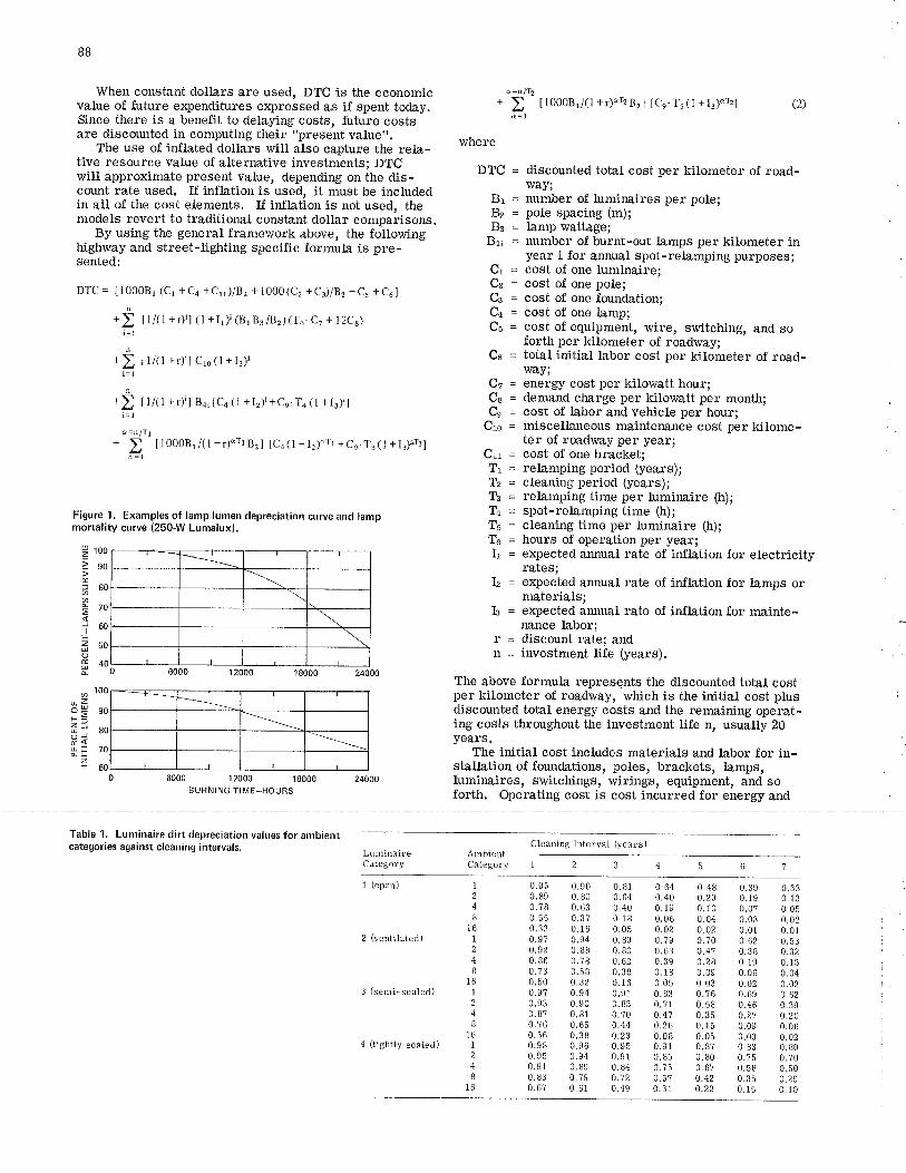
8B
When constant dollars are used, DT€ is the economicvalue of future e4penditures expressed as if spent today.Since tlere is a benefit to delaying costs, future costsare discounted in computing their 'þresent value".
The use of inflated dollars wilt also capture the rela-tive resource value of alternative investments; DTCwill approximate present value, depending on the dis-count rate used. If inflation is used, it must be includedin all of the cost elements. If inflation is not used, tlremodels revert to traditional constant dollar comparisons.
By using the general framework above, the followinghighway and street-lighting specific formula is pre-sented:
¡1ç = u000Br (cl +c4 +crr)/Bz + 1000(c2 +c3)/82 +cs +c6ln
+> tl/(1 +r)il (1 +Ir)i (BrB3/82)(T6. q + l2C8)i= I
n
+) tl/(l +r)ii cro(l +t3)ii= I
n
+t t1/(1 +r)il B+i [C4(1 +12)i+Ce.T4(l +13)i]i= I
d=n/Tl+ > [10008r/(l +r)orrBz] [C4(l +I2)"rr+Ca.T3(l +I3Frr]
q=1
Figure 1. Examples of lamp lumen depreciation curve and lampmortality curve (250-W Lumalux).
6000 r æ00 18000BURNING TIME_HOURS
e =n lT2+ ) tt000Br/(l+r)"r2B2l [ce.Ts(1+I3)ar2] Q)
where
DTC = discounted total cost per kilometer of road-way;
= number of luminaires per pole;= pole spacing (m);= lamp wattage;= nrmber of burnt-out lamps per kilometer in
year i for annual spot-relamping purposes;= cost of one luminaire;= cost of one pole;= cost of one foundation;= cost of one lamp;= cost of equipment, wire, switching, and so
forth per kilometer of roadway;= total initial labor cost per kilometer of road-
way;= energy cost per kilowatt hour;= demand charge per kilowatt per month;= cost of labor and vehicle per hour;= miscella¡eous mainteruùnce cost per kilome-
ter of roadway per year;= cost of one bracket;= relamping period (years);= cleaning period (years);= relamping time per luminaire (h);= spot-relamping time (h);= cleaning time per luminaire (h);= hours of operation per year;= e{pected annual rate of inflation for electricity
rates;= e4pected annual rate of inflation for Lamps or
materials;= expected arurual rate of i¡¡flation for mainte-
nance labor;= discount rate; and= investment life (years).
The above formula represents the discounted tot¿l costper kilometer of roadway, which is the initial cost plusdiscounted total energy costs and the remaining operat-ing costs throughout the investment life n, usually 20years.
The initial cost includes materials and labor for in-stallation of foundations, poles, brackets, lamps,luminaÍres, switchings, wirings, equipment, and soforth. Operating cost is cost incured for energy and
BrB¿
BsB¿i
CrCz
Ca
Ca,
Cs
Co
CzCe
GCro
CuTrT,TsT+TsT6Ir
1z
13
rn
z5tcfØØc
=J
IFzUoÉuÀ
LzF-z=U
E<HE
2
Table 1. Luminaire dirt depreciation values for ambientcategor¡es against cleaning intervals. Cleâning lnterval (years )
LuminaireCategory
AmbientCategorv
1 (open)
2 (ventilatecl)
3 (semi-sealed)
4 (tishtlv sealecl)
0.95 0.90 0.810.89 0.80 0,640.?8 0.63 0.400.55 0.37 0.180.32 0.16 0.050.9? 0.94 0.890.92 0.88 0.800.86 0.78 0.620.?3 0.58 0.380.50 0.32 0.1 6
0.9? 0.94 0.910.93 0.90 0.830.8? 0.81 0.700.?6 0.65 0.440.56 0.38 0.230.98 0.96 0.950.95 0.94 0.910.9 1 0. B9 0. 840.83 0.?9 0.'t20.6? 0.61 0.49
0.64 0.480.40 0.290.19 0.100.06 0.040.02 0.020.79 0.?00.63 0.4't0.39 0.280.18 0.090.05 0.030.83 0.760.71 0.580.4't 0.350.26 0.150.08 0.050.91 0.8?0. 85 0.800.?5 0.670.5't 0.420.31 0.22
0.39 0.330.19 0.130.0? 0.050.03 0.020.01 0.010.62 0.530.38 0.320.19 0.130.06 0.040.02 0.020.69 0.620.46 0.390.27 0.200.09 0.060.03 0.020.83 0.800.?5 0.?00.58 0.500.35 0.290.15 0.10
1
24
I16
1
2
4B
161
24B
161
24I
16
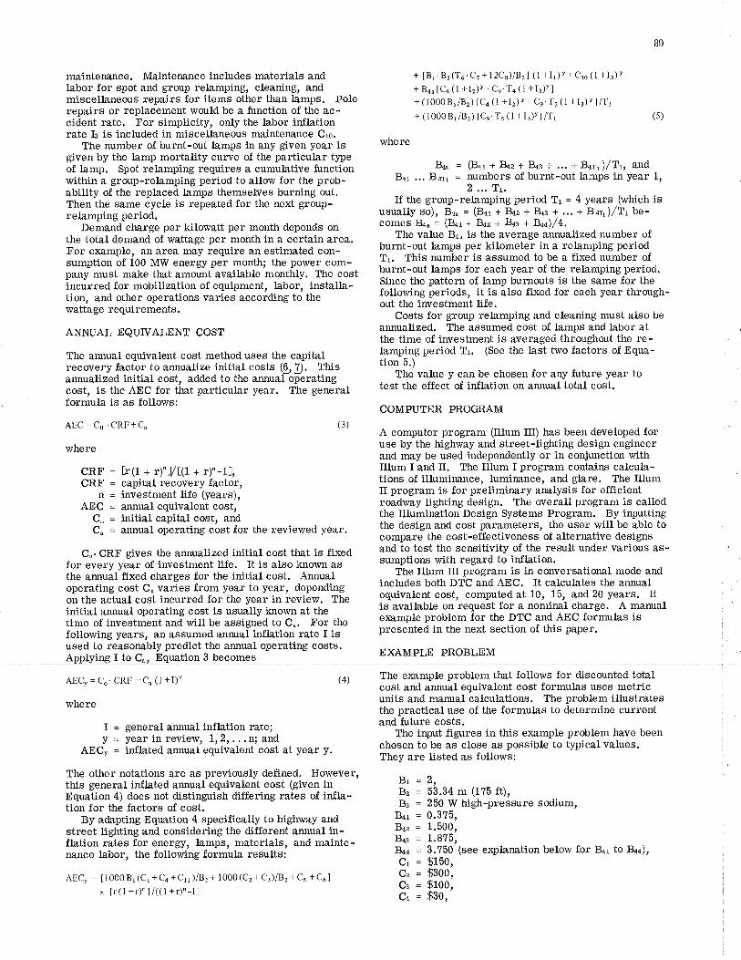
maintenance. Mainter¡ance includes materials andlabor for spot and group relamping, cleaning, andmiscellaneous repairs for items other than lamps. Polerepairs or replacement would be a function of the ac-cident rate. For simplicity, only the labor inflationrate I: is included in miscellaneous maintena¡ce Cro.
The number of burnt-out lamps in any given year isgiven by the lamp mortality curve of the particular typeof lamp. Spot reÞmping requires a cumulative functionwithin a group-relamping period to allow for the prob-ability of the replaced lamps themselves burning out.Then the same cycle is repeated for the next group-relamping period.
Demand charge per krlowatt per month depends onthe total demand of wattage per month in a certain area.For enample, an area may require an estimated son-sumption of 100 MW energy per month; the power com-pany must make thai amount available monthly. The costincurred for mobilization of equipment, labor, installa-tion, and other operations varies according to thewattage requirements.
ANNUAL EQUIVALENT COST
The arurual equivalent cost method uses the capitalrecovery factor to annualize initial costs ($ !). Thisannualized iaitial cost, added to the arutual operatingcost, is the AEC for that particular year. The generalformula is as follows;
AEC = Co .CRF+Cu
where
CRF = h(1 + r)"7[(1 + r)'-11,CRF = capital recovery factor,
n = investment life (years),AEC = a¡mual equivalent cost,
C. = initial capital cost, andC" = annual operating cost for the reviewed year.
C". CRF gives the annualized initial cost that is fixedfor every year of investment life. It is also known asthe ar¡nual fixed charges for the initial cost. Annualoperating cost C" varies from year to year, dependingon the actual cost incurred for the year in review. Theinitial armual operating cost is usually known at thetime of investment and will be assigned to C". For thefollowing years, an assumed annual inflation rate I isused to reasonably predict the arutual operating costs.ApplvinE I to C,. Equation 3 becomes
89
+ [Br. B3(T6. c1 + l2còlB2l (1 +Ir) v +cro (1 +13)v
+ 84â [C4 (l +12)v+ ce. T4 (1 +13)v ]+ fi 0008r/B:) [c¿ fi +Iz) v +cq. T¡ (1 +l¡)vl /Tr+(100081/82) [ca.Ts(l +I3)vllTr (5)
where
3n, = (B+r + B¿z + &s + ... +B+rr),/Ti, andB¿r ... Borr = numbers of burnt-out lamps in year 1,
2 ,.. TyIf the group-relamping period Tr = 4 years (which is
usually so), Bau = (Bar + B+z + B<¡ +... + B+r,)/Tr be-comes B,a. = (&r + B+z + B+a + B++)/4,
The value Be" is the average armualized number ofburnt-out lamps per kilometer in a relamping periodTr. This number is assumed to be a fixed number ofburnt-out lamps for each year of the relamping period.Since the pattern of lamp burnouts is the same for thefollowing periods, it is also fixed for each year through-out the investment life.
Costs for group relamping and cleaning must also beannualized. The assumed cost of lamps and labor atthe tíme of investment is averaged throughout the re-lamping period Tr. (See the last two factors of Equa-tion 5.)
The value y can be chosen for any future year totest the effect of inJlation on arurual total cost.
COMPUTER PROGRAM
A computer program (Illum ffi) has been developed foruse by the highway and street-lighting desiga engineerand may be used independently or in conjunction withIllum I and II. The Illum I program contains calcula-tions of illuminance, luminance, and glare. The lllumII program is for preliminary analysis for efÏicientroadway lighting design. The overall program is calledthe lllumination Design Systems Program. By inputtingthe design and cost parameters, the user will þe able tocompare the cost-effectiveness of alternative designsand to test the sensitivity of the result under various as-sumptions with regard to inflation.
The lllum III program is in conversational mode andincludes both DTC and AEC. It calculates the ar¡nualequivalent cost, computed at 10, 15, and 20 years. Itis available on request for a nominal charge. A manualexample problem for the DTC and AEC formulas ispresented in the next section of this paper.
EXAMPLE PROBLEM
(3)
AECy = Co.CRF + C" (l+I)Y @)
where
1 = general annual infl,ation rate;y = fear in review, L,2, .. .n' and
AECy = in-flated a¡nual equivalent cost at year y.
The other notations are as previously defined. However,this general inflated annual equivalent cost (given inEquatÍon 4) does not distinguish differing rates of infla-tion for the factors of cost.
By adapting Equation 4 specifically to highway andstreet lighting and considering the difïerent annual in-flation rates for energy, Iamps, materials, and mainte-nance labor, the following formula resultsl
AECy = il0008r(cl +c4+crl)/B2+ 1000(c2+c3)/B2+cs +c6lx [r(l +r)"]/[(l +r)'-1]
The example problem that follows for discounted totalcost and arurual equivalent cost formulas uses metricunits and manual calculations. The problem illustratesthe practical use of the formuLas to determine currentand future costs.
The input figures in this example problem t¡ave beenchosen to be as close as possible to typical values.They are listed as follows:
Bl=2,Bz = 53.34 m (1?5 ft),B. = 250 W high-pressure sodium,
B¿r = 0.375,B¿z = 1.500rBqs = L.876,B¿¿ = 3.750 (see explanation below for Bar to Be+),q, = 91b0,Cz = $800,g, = 9100,çn = 930,
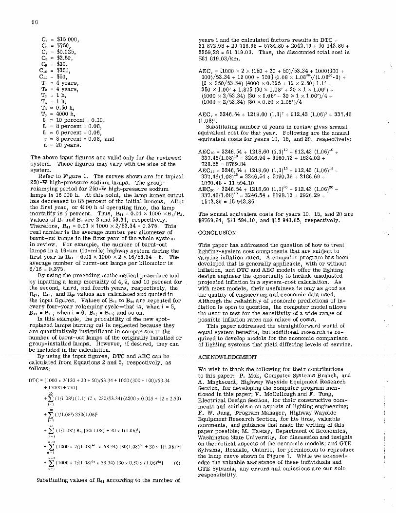
90
Cs = $15 000,Co = $750,Cr = $0.025,gu = 92.b0,gn = gB0,
Cro = $350,C" = $50,Tt = 4 years,Tz = 4 years,Ts = thrT+ = th,Ts = 0.50 h,To = 4000 h,L = 10 percent = 0.10,Iz = Spercent=0.08rIs = 6percent=0.06,r = Spercent=0.08, andn = 20 years.
The above input figures are valid only for the reviewedsystem. These figures may vary with the size of thesystem.
Refer to Figure 1. The curves shown are for typical250-W high-pressure sodium lamps. The group-relamping period for 250-W high-pressure sodiumlamps is 16 000 h. At this point, the lamp lumen outputhas decreased to 85 percent of the initial lumens. AJterthe first year, or 4000 h of operating time, the lampmortality is 1 percent. Thus, &r = 0.01 x 1000 xB/Bz.Values of Br and Bz Éùrê 2 and 53.34, respectively.Therefore, B¿r = 0.01 x 1000 x2/53.34 = 0.3?5. Thisreal numloer is the average number per kilometer ofburnt-out lamps in the first year of the whole systemin review. For example, the number of burnt-outlamps in a 16-km (10-mile) highway system during thefirst year is B'ar = 0.01 x 1000 x 2 x L6/53,34 = 6. Theaverage number of burnt-out Lamps per kilometer is6/16 = 0.3?5.
By using the preceding mathematical procedure andby inputting a þmp mortality of 4r5, and 10 percent forthe second, third, and fourth years, respectively, theBqz, Bcs, and Baa values are calculated and quoted inthe input figures. Values of B+r to Baa €!r€ repeated forevery four-year relamping cycle-that is, when i = 5,B+r = B¿r! when i = 6, B+t = B¿z; and so on.
In this example, the probability of t}te new spot-replaced lamps burning out is neglected because theyare quantitatively insignificant in comparison to thenumber of burnt-out lamps of the originally installed orgroup-installed lamps. However, if desired, they canbe included in the calculation.
years i and the calculated factors results in DTC =31 872.98 + 29 ?16.38 + 5784.80 + 2042.73 + 10 142.86 +2259.28 = 81 819.03. Thus, the discounted total cost is$81 819.03/km.
AEC" = t1000 x 2 x (150 + 30 + 50)/53.34 + 1000(300 +100)/$.34 + 15 000 + z50l (0.09 x 1.08'z0)/(1.0820-1¡ +
12 x 250/63.34) (4000 x 0.025 + 12 x 2.ã01 1.1v +350 x 1.06v+ 1.8?5 (30 x 1.08v+ 30 x 1 x 1.06v) +(1000 x 2/53.34) (30 x 1.08v + 30 x 1 xl.06v)/4 +(1000 x 2/53.34) (30 x 0.50 xr,06v)/4
AEC" = 3246.54 + 1218.60 (1.1)" + 9L2.43 (1.06)v + 337.46(1.08)v.
Substituting number of years in review gives annualequivalent cost for that year. Following are the ar¡nualequivalent costs for years 10, 15, and 20, respectively:
AECro = 3246.64 + 1218.60 (1.1)10 + 512.43 (1.06)10 +33?.46(1.08)1o = 3246.54 + 3160.?3 + 1634.02 +728.55 = 8769.84
AECrs = 3246,54 + 1218.60 (1.1)15 + 912.43 (1.06)15 +337.46(1.08)iu = 3246,54 + 5090.39 + 2186.69 +10?0.48 - 11 594.10
AECzo = 3246.54 + 1218.60 (1.1)20 + 912,43 (1.06)'z0 +33?.46(1.08)'z0 = 3246.54 + 8198.13 + 2926.29 +1572.89 = 15 943.85
The arurual equivalent costs for years 10, 15, and 20 are$8769.84, $11 594.10, and $15 943.85, respectively.
CONCLUSION
This paper lras addressed the question of how to treatlighting-system cost components that are subject tovarying inflation rates. A computer program has beendeveloped that is generally applicable, rvith or rvithoutÍnflation, and DTC and AEC models offer the lightingdesign engineer the opportunity to include unadjustedprojected ir¡flation in a system-cost calculation. Aswith most models, their usefuùress is only as good asthe quality of engineering and economic data used.Although the reliability of economic predictions of in-flation is open to questíon, the computer model allowsthe user to test for the sensitivity of a wide range ofpossible inflation rates and mixes of costs.
This paper addressed the straightfor"vard world ofequal system benefits, but additional research is re-quired to develop models for the economic comparisonof lÍghting systems that yield differing levels of service.
We wish to thank the following for their contributionsto this paper: P. Mok, Computer Systems Branch, andA. Maghsoudi, Highway Wayside Equipment ResearshSection, for developing the computer program men-tioned in this paper; V. McCullough and F. Tung,Electrical Design Section, for their constructive com-ments and criticism on aspects of lighting engineering;F. W. Jung, Program Manager, Highway WaysideEquipment Research Section, for his time, valuablecomments, and guidance that made the writing of tllispaper possible; M. Hastay, Department of Economics,Washington State University, for discussion and insightson theoretical aspects of the economic models; and GTESylvania, Rexdale, Ontario, for permission to reproducethe lamp curve shown in Figure 1. While we acknorvl-edge the valuable assistance of these individuals andGTE Sylvania, any errors and omissions are our soleresponsibility.
Bfusftg tfrnpuffrþures; ÐTC anal AEC cancalculated from Equations 2 and 5, respectively, asfollows:
p1ç = [1000 x 2(ls0 + 30 + 50)/53.34 + 1000 (300 + 100)/s3.34+15000+7501
20
+) itlt.osr){t,Ð1 Q x 250153.34)(4000 x 0.025 + 12 x 2.50)
20
+) tl/r.08i) 3s00.06)¡
20
+ ) {r/l.oat) B4i [30(1.08)i+ 30 x l(1.06)i]i= I
a=s+ ) (1000 x 21u.08)e x 53.34) t30(1.08)4" + 30 x 1(1.06)a.l
a=s+ > (1000 x 2/(1.08)a"x 53.34) t30 x 0.50 x (1.06)4"1 (6)
Substituting values of B+r ¿ùccording to the number of
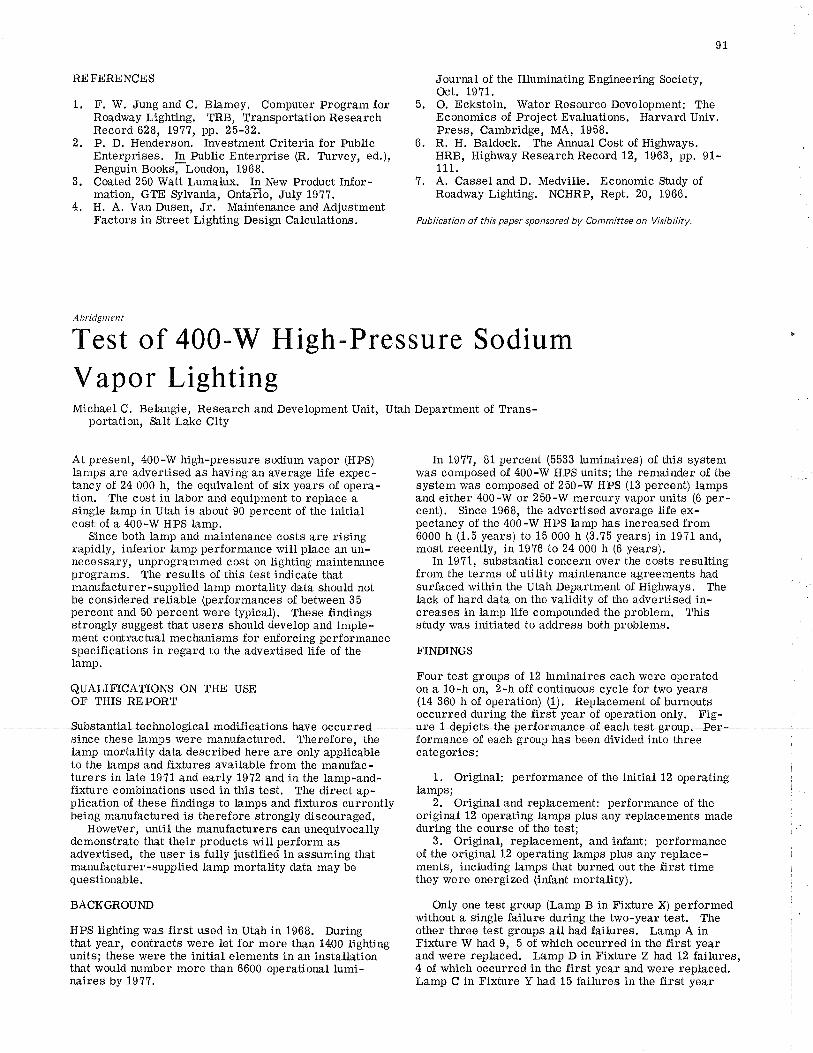
91
REFERENCES
1. F. W. Jung and C. Blamey. Computer Program for
Journal of the Illuminating Engineering SocÍety,Oct.19?1.
5. O. Eckstein. \üater Resource Development: The
3.
4.
Record 628, t977, pp. 25-32.2. P. D. Henderson. Investment Criteria for Public
Enterprises. In Public Enterprise (R. Ttrvey, ed,),Penguin Books, London, 1968.Coated 250 Watt Lumalux. In New Product lrfor-mation, GTE Sylvania, Ontaão, JuIy 19??.H. A. Van Dusen, Jr. Maintenance and AdjustmentFactors in Street Lighting Desiga Calculations.
Abridgntent
Press, Cambridge, MA, 1958.6. R. H. Baldock. The A¡u¡ual Cost of Highways.
HRB, Highway Research Record 12, 1963, pp. 91-111.
7, A, Cassel and D. Medville. Economic Shrdy ofRoadway Lighting. NCHRP, Rept. 20, 1966,
Publication of this paper sponsored by Committee on Visibility.
since these lamps were manufactured. Therefore, thelamp mortality data described here are only applicableto the Lamps and fixtures available from the manufac-turers in late 1971 and earLy 1972 and in the lamp-and-fixture combinations used in this test. The direct ap-plication of these findings to lamps and fixtures currentlybeing manufactured is therefore strongly discouraged.
However, until the manufacturers can unequivocallydemonstrate that their products wiII perform asadvertised, the user is fully justified in assuming thatmanufacturer-supplied lamp mortality data may bequestionable.
BACKGROUND
HPS lighting was first used in Utah in 1968. Duringthat year, contracts were let for more than 1400 lightingunits; these were the initial elements in an instalþtionthat would number more than 6600 operational lumi-naires by 197?.
Ín 19'17, 81 percent (5533 luminaires) of this systemwas composed of 400-rvV HPS units; the remainder of thesystem was composed of 250-W HPS (13 percent) lampsand either 400-W or 250-W mercury vapor units (6 per-cent). Since 1968, the advertised average life ex-pectancy of the 400-W HPS lamp has increased from6000 h (1.5 years) to 15 000 h (3.?5 years) in 1971 and,most recently, in 19?6 to 24 000 h (6 years).
In 1971, substantial concern over the costs resultingfrom the terms of utitity maintenance agreements hadsurfaced within the Utah Department of Highways. Thelack of hard data on the validity of the advertised in-creases in lamp life compounded the problem. Thisstudy was initiated to address both problems.
FINDINGS
Four test groups of 12 luminaires each were operatedon a 10-h on, 2-h off continuous cycle for two years(14 360 h of operation) (1). Replacement of burnouts
formance of each group has been divided into threecategories:
1. Original: performance of the initial 12 operatinglamps;
2. Original and replacement: performance of theoriginal 12 operating lamps plus any replacements madeduring the course of the test;
3. Oríginal, replacement, and infant: performanceof the original 12 operating lamps plus any replace-ments, including Lamps that burned out the first tÍmethey were energized (in-fant mortality).
Only one test group (Lamp B in Fixture X) performedwithout a single failure during the two-year test, Theother three test groups all had failures. Lamp A inFixbure W had 9, 5 of which occurred in the first yearand were replaced. Lamp D in Fixture Z had 12 failures,4 of which occurred in the first year and were replaced.Lamp C in Fixture Y had 15 failures in the first year
occurred during the first year of operation only. Fig-ialJeehnologieal msdifi-eations ha+e oee+ered- ++#cpietslhe performa+rec sf caeh test4-oup- +õ+- 1
Test of 400-W High-Pressure SodiumVapor LightingMichael C. Belangie, Research and Development Unit, Utah Department of Trans-
portation, Salt Lake City
At present, 400-W high-pressure sodium vapor (HPS)lamps are advertised as having an average life ex¡lec-tancy of 24 000 h, the equivalent of six years of opera-tion. The cost in labor and equipment to replace asingle lamp in Utah is about 90 percent of tlte initialcost of a 400-W HPS Þmp.
Since both lamp and maintenance costs are risingrapidly, in-ferior lamp performance rvill place an un-necessary, unprogrammed cost on lighting maintenanceprograms. The results of this test indicate thatmanufacturer-supplied lamp mortality data should notbe considered reliable þerformances of between 35percent and 50 percent were typical). These findingsstrongly suggest that users should develop and imple-ment contractual mechanisms for enforcing performancespecifications in regard to the advertised life of thelamp.
QUALIFICATIONS ON THE USEOF THIS REPORT
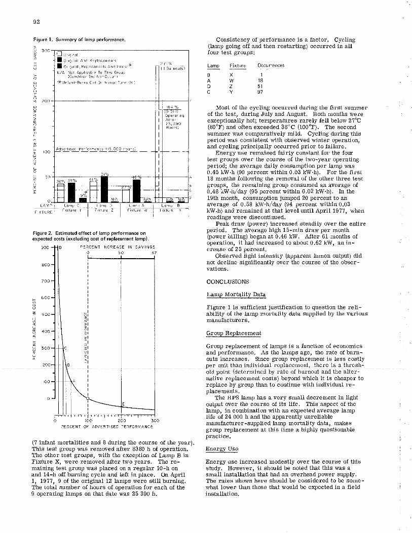
92
Figure 1. Summary of lamp performance. Consistency of performance is a factor. Cycling(lamp going off and then restarting) occurred in allfour test groups:
lo,'n'"o,,RpptocemenrsAndtnfont* n#!#""rr,N/A Not ApÞlrcoble To Thrs Group
(Condrlro¡ Drd Not'Occur )
ì( {lnfonl=Burns Out On lnrlrol lurn On)
A!vl!.ls:jlPg.llgrgnce ( l5,ooo Hours) _
OperoirngAfter25,390Hours)
LompC I LompD I LompA I Lomo B
o3 3oo
tsØts
moUtrl-? zoo
B
D
c
Lamp Fixture Occurrences
Most of the cycling occurred during the first summerof the test, during July and August. Both months wereexceptionally hot; temperatures rarely fell below 2?oC(BOoF) and often exceeded 38'C (100T'). The secondsummer was comparatively mild. Cycling during thisperiod was consistent with observed winter operation,and cycling principally occurred prior to failure.
Energy use remained fairly constant for the fourtest groups over the course of the two-year operatingperiod; the average daily consumption per lamp was0.45 kw.h (90 percent within 0.03 kw.h). For the first18 months following the removal of the other three testgroups, the remaining group connumed an average of0.48 kW.h/day (95 percent within 0.02 kw.h). In the19th month, consumption jumped 20 percent to anaverage of 0.58 kw'h/day (94 percent r¡¡ithirl 0.03kW.h) and remained at that level until April 1977, whenreadings were discontinued.
Peak draw þower) increased steadily over the entireperiod. The average high 15-min draw per monthþower bilting) began at 0.46 kW, After 61 months ofoperation, it had increased to about 0.62 kW, an in-crease of 25 percent.
Observed light intensity (apparent lumen output) didnot decline significantly over the course of the obser-vations.
CONCLUSIONS
Lamp Mortality Data
Figure 1 is sufficient justification to question the reli-ability of the lamp mortality data supplied by the variousmanufacturers.
Group Replacement
Group replacement of lamps is a function of economicsand performance. As the lamps age, the rate of burn-outs increases. Since group replacement is less costly
1
1851
97
XWzY
oz
EoÉUIôUØ
L tOOuoLot50(Uû
oLA lvl P
Figure 2. Estimated effect of lamp performance onexpected costs (excluding cost of replacement lamp).
ulol2,
=lÉolÉlul
olUIolÀl
. 600ØooZ sooU
U$ +oozFz3 3ooÉUÀ
PERCENT INCREASE IN SAVI NGS
o5067
o r00 200 300PERCENT OF ADVERTISED PERFORMANCE
(7 infant mortalities and I during the course of the year).This test group was removed after 8380 h of operation.The other test groups, with tl¡e exception of Lamp B inFixhrre X, were removed a-fter two years. The re-maining test group was placed on a regular 10-h onand 14-h off burning cycle and left in place. On April1, L977, 9 of the original 12 lamps were still burning.The total number of hours of operation for each of the9 operating lamps on that date was 25 390 h.
r unit than individual there is a thresh-old point rmined by rate of burnout and the alter-native replacement costs) beyond which it is cheaper toreplace by group than to continue with individual re-placements.
The HPS lamp has a very small decrement in lightoutput over the course of its life. This aspect of thelamp, in combination with an enpected average lamplife of 24 000 h and the apparently unreliablemanufacturer -supplied lamp mortality data, makesgroup replacement at this time a highly questionablepractice.
Energy Use
Energy use increased modestly over the course of thisstudy. However, it should be noted that this was asmall installation that had an overhead power supply.The rates shown here should be considered to be some-what lower than those that would be e4pected in a fieldinstallation.
Demand
Peak energy demand þower) rnay play a role in lightingcosts in areas where penalties are placed on users whocontribute to peat demand.
IMPLEMENTAflON
Figure 2 indieates the effect of Lamp performance onthe expected cost of maintenance. Points A through Erefer to the'equivalent reference lines drawn on the rightvertícal of Figùre 1. In a lightíng system composed oflamps performingat 50 percent of advertised capability(reference line A in Figure 1) that were replaced atburnout with Þmps of equivalent operational (as opposedto advertised) capability, the qost of maintaining thesystem would be 100 percent greater þoint A in Figure2) than the amount budgeted for the time period. Inrelating Figure 1 to Figure 2, ít can be seen that theperformance of the first three groups in Figure 1 couldhave raised the e4pected maintenance cost of a lightingsystem composed exclusively of those lamps and fix-tures by 100-900 percent of the e¡pected cost.
In considering the fourth group in Figure 1 (Lamp B,Fixture X) and relating reference line E in Figure 1
to point E in Figure 2, it would appear that this com-bination would yield substantial savings. However, ifa group replacement policy that was based on themanufacturer's lamp mortality data had been in effect,then the indicated savings would not have been realized;the lamps would have been repl,aced in groups at ap-proximately 92 percent of theír advertised life (13 800 h).It must be noted that in 197? no major lamp manufac-turer recommended group replacement of HPS l;amps.
It is apparent that the users must find some methodto protect themselves from manufacturers of in-terior
93
products. The low-bid requirement, in an area such aslamp purchases, c¿Ln cause a user to incur a substantialmaintenance liability through the mandatory purchaseof a less than satisfactory product.
The city of Seattle (Ð attd the state of ldaho Q) haveused a life-cycle costing approach to implement apartial solution to this problem. rvVhether their ap-proach is adequate is yet to be determined.
In order to achieve the savings indicated in Figure 2,group replacement that is based on manufacturer-supplied data must be eliminated in favor of either re-placement a-fter individual burnout or a group replace-ment system that is based on in-house data. Theeconomic feasibility of the latter apprech is question-able and needs to be evaluated before serious thoughtis given to its implementation.
The potential benefits of this study will be largelydetermined by the effectiveness of the steps taken byusers to require performance at the level advertised.
REFERENCES
1. M. C. Belangie. 400-Watt High-Pressure SodiumVapor Lighting Test (15 000-Hour Lamp Rating),Executive Summary. Utah Department of Trans-portation, Salt Lake City, Final Rept., July 1977.
2. B. Bermack. Cost Analysis of High-IntensityDischarge Mercury Vapor and High-PressureSodium Lamps, 1975 Annual Contract. City ofSeattle, Seattle, Washington, 1975.
3. Bid Invitation for Electric Lamps for Slate of ldahoAgencies. Idaho Division of Purchasing, Boise,llÍay 27, L917.
Publication of this paper sponsored by Comm¡ttee on Visibility.
Abidgment
During FogFrank D. Shepard, Virginia Highway and Transporlation Research
CouncilJharlottesv
Pavement Inset Lights for Use
Reduced visibility as a result of fog presents a veryhazardous condition on the highway because motoristsare unable to readily observe pavement markings andsigns and the movement of tra-ffic. Afton Mountain,which is traversed by I-64, is often the site of suchreduced visibility because of the low cloud cover onthe mountaintop during rainy periods.
An acute awareness of the fog problem on AftonMountain led to a decision by the Virginia Departmentof Highways and Trarsportation to install a lightingsystem that consists of pavement inset lights and low-level illumination lights to aid motorists during periodsof fog. The installation was made on a 9.3-km (5.8-mile) section of highway that encompasses the top ofAfton Mountain. Since fog often occurs on only a por-tion of the mountain, the installation was divided intothree sections that represent the points observed tomost often correspond rvith the fog patterns. Each
section is controlled by two fog detectors, located ator close to the endpoints of t}te sectíon, that arecapable of detecting five levels of fog density. Theintensity of the guidarce lights within each section iscontrolled by the density of the fog at each detector.
The fog guidance system consists of unidirectionalairport runway lights installed in the pavement edgeline along each side of the roadrvay in both directions,spaced at 61-m (200-ft) intervals on tangent sectionsand 30.ã-m (100-ft) intervals on curved sections. Inaddition to the white inset lights on the main line, amberlights are installed on one side of the off-ramps. Also,low-level illumination lights are installed on a shortsection of an on-ramp.
It was felt that the lighting system would helpdelineate the highway atd thus lead to an improvementin tra-tfic operations. However, it was not known howthe system of lights would a-ffect vehicle speeds, head-
automobiles in the tra^ffic lane in the a-fter period. Re-Data were collected before (Il/27h3-5/l/76) and a-fter sults for the remainder of the comparisons showed no(L/26/76-S/30/76) installation of the lighting system differences for automobiles or traðtor-trailers, withby using tape switches placed on the highway. Under the exception of automobiles in the passing tane for acle?r, dry_conditions the tape switches were attached sight-distance interval of 33.5-45.7 m (110-1õ0 ft)to the road surface with double-faced tape. During a"t¡ead of the data collection point. The decrease inadverse weather, they were attached to 0,56-mm daytime speeds is e4plained by the fact that during day-(0.022-in) metal ribbons stretched across the highway light hours, within the range of sight distances en-ar astened to rnetalãrchorsìn theslroutderandmedian. three centerline skips 1I2,2-m (40-ft) intervals; 4.6-m
Data from all the tape switches were recorded si- (15-ft) painted linel; however, the uniqueness of themultaneously on a four-clrannel chart recorder; the system, in addition to some gtare assõciated with thes\¡¡itches were identified by assigning different voltages lights, caused the motorist to slow down. It is feltto each. Since the dista¡ce betrveen the tape switches on that when the data were accumulated the inset lightsthe road and the speed of tlre chart recorder were lvere a little brighter than they needed to be, whichknown, vehicular speeds and headways were determined caused the glare and deceleration, and that, once ex-by measuring the distances between impulses on the perience allows a realistic coordination between thechart. sight distances in fog and light intensÍties, speeds wilt
Vehicle placements were obtained by installing tape tend to be closer to those found in the before conditions.
94
ways, and placement. Also, there was some concernthat the system might promote a false sense of securityand lead to higher speed and greater differentials inspeed, which would increase the possibility of accideuts.It was, therefore, the purpose of this research to in-vestigate the tra-ffic flow characteristics during fogwithin the system of pavement inset lights installed onAfton Mountain.
The scope of the study included the collection andanalysis of trafïic flow data before and a-fter the lightswere installed. The parameters evaluated were ve-hicle speeds, headways, queues, and lateral placement.A before-and-a-fter accident analysis was also made.Because of the variability of fog densities for the periodof study a¡d the Iimitations on the time, persormel, andfunding allocated for the study, it was not possible tocollect tra-ffic flow data for all fog conditions.
METHOD
The effect of the system of lights on the tra-ffic ftowcharacteristics was determined by comparing data col-lected before and a-tter the system was installed. Datawere collected for all fog conditions (day and night)occurring during the time allowed for the project. Thecollection of data was limited to weekdays and to off-peak hours.
For the accident study, data were obtained from theDivision of Motor Vehicles.
Site
One location on the two westbound lanes of I-64 overAfton Mountain just east of the Blue Ridge Parkway waschosen for data collection. This location, which hadan annual average daily tra^tfic count of approximately5000 vehicles for the period 1973-L916, is on the levelsection of the mountaintop and has a slight horizontalcurve to the right. There are no interchanges inadvar¡ce of the site for a distar¡ce of 11.3 km (? miles).Data were collected at only one site.
Collection of Data
switches of different lengths on the right edge of thetra-ffic lane and noting which switch combinations were
Weather Conditions
The fog problem considered is one caused by low cloudcover in the mountainous areas. Although the fogs arerelatively dense urd uniform, variable fog conditions,fog banks, a¡rd so on do occur at the edges of the cloudcover and in areas under broken clouds that result fromclearing weather. For the evaluation, data were takenonly during uniform fog conditions extending at least152.4-304.8 m (500-1000 ft) in advance of the test site.
Fos Densitv
It was very important that a relative measure of fogdensity be obtained, because this influences tra-ffic flowcharacteristics. The density was determined by notingthe number of visible centerline stripes on the pave-ment during daylight hours a¡d the number of reflec-torized shoulder delineators during hours of darkness.These distances were used to identify relative fogdensities in the analysis of the data.
Since the tape switches were approximately 304.8 mfrom the data recorders, the fog densities and theuniformity of the fog were monitored by driving throughthe site at regular intervals.
RESULTS
The numerous variables associated with the project,problems encountered in data co[ection during adverseweather conditions, and the time frame in which it waspossible to collect the data limited the quantity of datacollected. Therefore, the study results reflect onlythose data for which comparable before-a¡rd-a-fterconditions were available.
Speeds
The installation of the pavement inset Iights has re-sulted in a decrease in daytime speeds and an increasein nighttime speeds. For all tireìigirt distances testedin fog during daytime and nighttime, there was asignificant increase ín the variability of speeds for
Daytime fog creates restrictive driving conditions;however, it is during nighttime fog that driving becomes
activated. difficult, primarily because of the driver's inabilityThe chart recorder was placed in a vehicle parked to see pavement markings and delineators whose
approximately 304.8 m (1000 ft) past the site to eliminate retroreflectivity is significantly reduced under nightany influence the parked vehicle may have had on tra-tfic or wet-weather conditions. Also, the reflection of theflow. Also, the switches were not conspicuous to vehicle's headlights from the fog seriously restricts
the motorist's visibility. The significant increases inspeeds ùrring nighttime fog give strong support to thecontention that the inset lighting system provides
motorists.
additional delineation for guidance. However, it shouldbe noted that the increase in speed at night for the a-ftercondition increases the accident potential, since eventhe nighttime speeds before installation exceed thoserequired for a safe stopping distance.
Sa^fe Stopping Distance
For all conditions investigated (before and after), theactual sight distances were less tha¡ the sa-fe stoppingdistances, a finding that indicates that drivers tend togo too fast for sight distances in fog, It is noted abovethat the increase in nighttime speeds since the installa-tion of the lights raises the accident potential as a re-sult of the increased stopping dista¡rces required. How-ever, the low tra-ffic volume encountered on this ruralsection of Interstate highway, especially at night, leadsto a decrease in vehicle interaction that lessens thesignificance associated with the safe stopping distance.Also, the improved delineation is thought to helpprevent vehicle stoppages along the roadway.
Headways
A review of the headway data showed little difïerencein headways between the before and a-fter conditionsduring the hours of daylight. However, available datashowed a decrease in nighttime headways (below 3 s)a-fter the inset lights were installed. This finding,coupled with results that showed less vehicle queuing inthe after condition, indicates that motorists were usingthe inset lÍghts for guidance rather than relying on carfollowing.
Queuing
There was a deerease in daytime vehicle queuing for thesight distance of 33.5-45.7 m (110-150 ft) but little dif-ference within the range of 45.?-61.0 m (150-200 ft). Atnight, for both sight distances considered, there was adecrease in vehicle queuing. There was little difference
95
in the numbers of vehicles in the queues. The increasein headways a¡d decrease in vehicle queuing at nightmight indicate a reduction in tìe potential for accidentsunder the lighting system. However, it should be notedthat, for severely restricted sight distances before thesystem was Ínstalled, vehicles tended to form queuesfor the purpose of being led through the fog, which maybe thought of as being safer than having no one to follow.
Lateral Placement
During daylight, the lateral placement of automobileswas farther from the right edge line a-fter the lights wereinstalled. Also, the placement was farther from theedge line during fog for both the before and after periodstha¡ it was during clear weather conditions. Both auto-mobiles and tractor-trailers were positioned fartherfrom the edge line for nighttime fog conditions than forclear conditions.
Accidents
It would be difficult to surmise what, if any, Íncreasein accident potential would result from the differencesnoted in traffic flow parameters. There has loeen onlyone accident during fog conditions since the system oflights was installed. Also, in a recent subjectiveevaluation of the system, more tltan 95 percent of themotorists intervíewed indicated that they were aidedby the system and 90 percent reported that the lightsreduced their anxiety while driving in fog (!.
REFERENCE
1. M. F. Creech and T. A, Crisman. Evaluation of the5.8-Mile Highway Light System for Guidance in Fogon Afton Mountain. Virginia Highway and Trans-portation Research Council, Charlottesville, Sept.1976.
Publication of this paper sponsored by Committee on Visibility.
Driver Performance with Right-Side
Ronald R. Mourant, Oakland University, Rochester, MichiganRobert J, Donohue, General Motors Corporation, Warren, Michigan
The mirror-use behavior of drivers was invest¡gated as they gathered ¡n-format¡on from rearview mirrors in order to execute freeway lanechanges and merges. Nine drivers (three novice, three experienced, andthree mature) drove a 1973 Buick LeSabre with and without a right-s¡defender-mounted convex mirror along a 22.5-km (14-mile) freeway route.The total time to obta¡n information per maneuver was the same forboth cases. ln a subsequent study, the mirror-use behavior of five sub-
¡ects who drove a 1976 Nova without a r¡ght-side convex mirror wascompared w¡th that of 12 subjects who drove the same veh¡cle with aright-side door-mounted convex mirror. Again there were no differencesin total t¡me to obtain rear-vision information. Experienced drivers(mean age = 24) took less time to obtain information when a right-sideconvex mirror was available than when it was not; older drivers (meanaSe = 61 ) took more time. Also, experienced drivers required about 10h of driving experience to become efficient users of a right-side convexmirror, while older drivers required considerably more driving experience,
Finally. a comparison of right-side door- and fender-mounted convexmirrors indicated that the drivers'total time to obta¡n ¡nformat¡on wasthe same for each mounting location, but drivers who had the fender-mounted mirror made a greater number of direct looks to the rear.
Some drivers may find it difficult to obtain the properinformation necessary to execute lane changes andmerges to the right. Factors that contribute to this dif-ficulty include the following: (a) plane mirrors locatedon the right door do not always provide an adequate fieldof view, (b) sail panels located at the right rear of thevehicle can obstruct vision, (c) high head restraints canrestrict the vision of short drivers, and (d) physical af-flictions and old age can restrict turning one's head to
96
Table 1. Subjects' ages and distancesdriven, by groups.
Group 1 Group 2 Group 3 Group 4
DistanceAge Driven(years) (km 000s)
DistanceAge Driven(years) (km 000s)
DistanceAge Driven Age(years) (kn 000s) (years)
DistanceDri ve n(km 000s)
1
2J
4567
B
I1011
t2
162126
¿a424851
4.00.85.6
113130't2
320400560
20 \2023 8024 24047 48069 480
l7 55 21 3918 40 27 32020 24 22 9720 48 23 482t 48 23 9?21 320 54 8043 390 55 16044 160 58 7249 48 60 8054 80 61 14060 80 62 16063 800
Note: I km = 0.6 mile.
make direct looks to the rear, use of the right-side convex mirror, Older, matureOne way to improve right-rear vision is to mount a drivers have ingrained information-gathering habits and
convex mirror on the right side of the vehicle. A convex therefore will probably take a longer time to become ac-mirror of relatively small size [13.3 cm (5,25 in) widel customed to the convex mirror. Even though olderand moderate radius of curvature [102 cm (40 in)] will drivers, in general, have poorer vision than youngerprovide an adequate field of view (19-200) for detecting drivers, the location of the convex mirror on the rightvehicles located at the right rear of the vehicle. For side of the vehicle places it far enough away from thecalculation of field-of-view requirements, see Sugiura driver so as to eliminate the necessity for large changesand Kimura (1). in eye accommodation (as well as reducing the need for
Since the r-adius of curvature of a convex mirror is a head turn to the rear), Thus, as noted by Seeser (10),less than infinity, objects appear smaller than they would older drivers will not need corrective lenses to view-ÏÏ,in a plane mirror. The viewing of these minified objects 3. How long does it take drivers to learn to use con-may result in erroneous distance judgments; that is, vex mirrors? Since little is currently known about howdrivers may judge vehicles to be located further to the drivers use a right-side convex mirror as a detectionrear than they actually are. Several investigators have device, especially how it is used in conjunction with in-studied this problem (\-! ana have found that drivers side mirror glances, it may be difficult to tell whencan misjudge distances when they use convex mirrors. drivers have become highly skilled convex-mirror users.Walraven and Michon (4) reported that experienced However, since skill learning improves rapidly duringdrivers would accept s-maller traffic gaps than inexperi- the early part of training, it will be possible to detectenced drivers, suggesting that judgment would improve when a learning plateau has been reached.with training. Also, Mortimer (5) found that, when 4. Does the location of the right-side convex mirrordrivers use the inside mirror inionjunction with an out- (door or fender mounted) affect the method and durationside convex mirror, misjudgments in distance do not of information gathering? A door-mounted convex mÍr-
"go or no-go. device (Q), distance judgments are irrele- more information, A fender-mounted mirror, on thevant. In a "go or no-gõ" situation, a driver simply uses other hand, requires only slight eye movement fromthe convex mirror to detect a vehicle's presence. If no straight ahead. If the fender- and door-mounted mir-vehicle is present, the driver proceeds with the maneu- rors are of the same size and convexity, their fields of
occur.Furthermore, when a convex mirror is used as a
ver, If a vehicle is present, the driver checks its ac-tual location by using the inside mirror or by a directlook to the rear.
drivers executed left and right maneuvers in freewayand city traffic. They found that when a right-sidefender-mounted convex mirror was available driversmade fewer direct looks to the side or rear of the ve-hicle than when it was not available.
Questions to be answered by means of the presentresearch include the following:
1. How does the information-gathering behavior ofdrivers change when a right-side convex mirror is avail-able? Will drivers use the convex mirror in actual traf-fic situations, and will they take more or less time toobtain information? A survey by Kaehn (8) found thatdrivers of government vehicles who used?ight-hand con-vex mirrors were impressed by the improved field ofview,
2, Does convex-mirror-use behavior differ accord-ing to the age of the driver? As Mourant and Rockwell(9) reported, young novice drivers make very little useof the left-side mirror and hence are likely to make little
ror requires a greater head turn from straight ahead,and it permits the use of peripheral vision to obtain
view will be about equal.5. Does information obtained prior to the decision
to execute a lane change affect subsequent information-
the ilmemory effect" of inlormation obtained prior tomaking a decision would be fairly short. This questionwas addressed mainly for methodological considerations.If there is no memory effect, different mirror systemsmay be compared by having drivers sample their mir-rors whenever desired (the natural driving method).However, if there is a memory effect, then mirrorsshould be sampled only after the decision to make a lanechange has been reached,
METHOD
Drivers
Table 1 shows the ages and distances driven for the foursubject groups. All drivers had valid Michigan licensesand at least 20/40 visual acuity.
Burger and others (? have collected data on driversr gathering strategy? Realization that a vehicle is moving
-l.¿nee behador¡¡¡ith.c&vermi¡ror systemrwhile the ttrrougù atonstantlythangingenvÍronnrenfsuggeststhat-
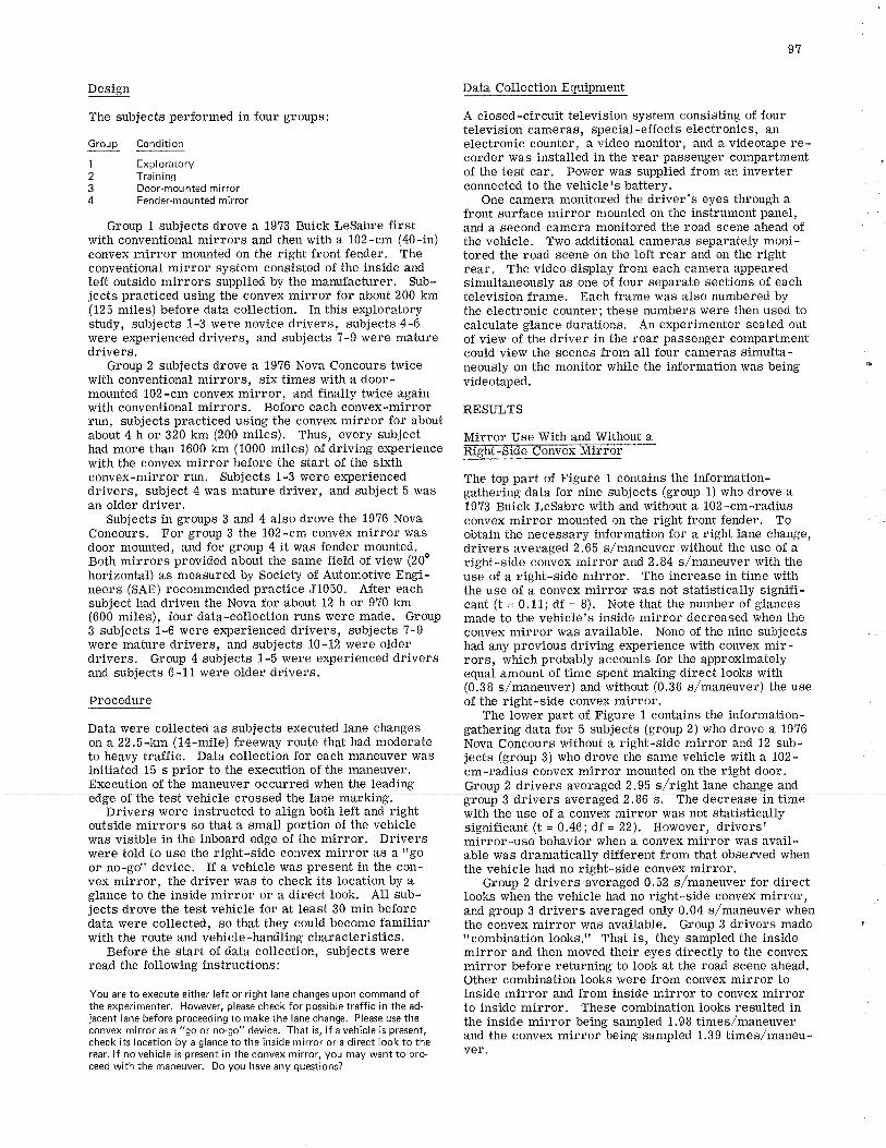
Design
The subjects performed in four groups:
Group Condit¡on
1 Exploratory2 Training3 Door-mounted mirror4 Fender-mounted mirror
Group 1 subjects drove a 19?3 Buick LeSabre firstwith conventional mirrors and then with a 102-cm (40-in)convex mirror mounted on the right front fender. Theconventional mirror system consisted of the inside andIeft outside mirrors supplied by the manufacturer. Sub-jects practiced using the convex mirror for about 200 km(125 miles) before data collection. In this elploratorysfudy, subjects 1-3 were novice drivers, subjects 4-6were experienced drivers, and subjects 7-9 were maturedrivers,
Group 2 subjects drove a 1976 Nova Concours twicewith conventional mirrors, six times with a door-mounted 102-cm convex mirror, and finally twice againwith conventional mirrors. Before each convex-mirrorrun, subjects practiced using the convex mirror for aboutabout 4 h or 320 km (200 miles). Thus, every subjecthad more than 1600 km (1000 miles) of driving experiencewith the convex mirror before the start of the sixthconvex-mirror run, Subjects 1-3 were experienceddrivers, subject 4 was mature driver, and subject 5 wasan older driver,
Subjects in groups 3 and 4 also drove the 1976 NovaConcours, For group 3 the 102-cm convex mirror wasdoor mounted, and for group 4 it was fender mounted.Both mirrors provided ã¡out tire same field of view (20o
horizontal) as measured by Society of Automotive Engi-neers (SAE) recommended practice J1050. After eachsubject had driven the Nova for about 12 h or 970 km(600 miles), four data-collection runs were made. Group3 subjects 1-6 were experienced drivers, subjects 7-9were mature drivers, and subjects 10-12 were olderdrivers. Group 4 subjects 1-5 were e4perienced driversand subjects 6-11 were older drivers.
Procedure
Data were collected as subjects executed lane changeson a 22.5-km (14-mile) freeway route that had moderateto heavy traffic. Data collection for each maneuver wasinitiated 15 s prior to the execution of the maneuver.Execution of the maneuver occurred when the leading
97
Data Collection Equipment
A closed-circuit television system consisting of fourtelevision cameras, special-effects electronfcs, anelectronic counter, a video monitor, and a videotape re-corder was installed in the rear passenger compartmentof the test car, Power was supplied from an inverterconnected to the vehicle's battery.
One camera monitored the driver's eyes through afront surface mirror mounted on the instrument panel,and a second camera monitored the road scene ahead ofthe vehicle. Two additional cameras separately moni-tored the road scene on the left rear and on the rightrear, The video display from each camera appearedsimultaneously as one of four separate sections of eachtelevision frame, Each frame was also numbered bythe electronic counter; these numbers were then used tocalculate glance durations. An experimenter seated outof view of the driver in the rear passenger compartmentcould view the scenes from all four cameras simulta-neously on the monitor while the information was beingvideotaped.
RESULTS
Mirror Use With and Without a@The top part of Figure 1 contains the information-gathering data for nine subjects (group 1) who drove a1973 Buick LeSabre with and without a 102-cm-radiusconvex mirrot mounted on the right front fender, Toobtain the necessary information for a right lane change,drivers averaged 2.65 s/maneuver without the use of aright-side convex mirror and 2.84 s/maneuver with theuse of a right-side mirror. The increase in time withthe use of a convex mirror was not statistically signifi-cant (t = 0.11; df = B), Note that the number of glancesmade to the vehicle's inside mirror decreased when theconvex mirror was available, None of the nine subjectshad any previous driving ex¡lerience with convex mir-rors, which probably accounts for the approximatelyequal amount of time spent making direct looks with(0.38 s,/maneuver) and without (0.36 s/maneuver) the useof the right-side convex mirror.
The lower part of Figure 1 contains the information-gathering data for 5 subjects (group 2) who drove a 1976Nova Concours without a right-side mirror and 12 sub-jects (group 3) who drove the same vehicle with a 102-cm-radius convex mirror mounted on the right door,
Drivers were instructed to align both left and ríghtoutside mirrors so that a small portion of the vehiclewas visible in the inboard edge of the mirror. Driverswere told to use the right-side convex mirror as a "goor no-go" device. If a vehicle was present in the con-vex mirror, the driver was to check its location by aglance to the inside mirror or a direct look. All sub-jects drove the test vehicle for at least 30 min beforedata were collected, so that they could become familiarwith the route and vehicle-handling characteristics.
Before the start of data collection, subjects wereread the following instructions:
You are to execute e¡ther left or right lane changes upon command ofthe experimenter. However, please check for possible traffic in the ad-jacent lane before proceeding to make the lane change, Please use theconvex mirror as a "go or no-go" device. That is, if a vehicle is present,check its location by a glance to the inside mirror or a direct look to therear. lf no vehicle is present in the convex mirror. you may want to pro-ceed with the maneuver. Do you have any questions?
2 drivers ave 2.95 s/right lane change andgroup rs aver se rn trmewith the use of a convex mirror was not statisticallysignificant (t = 0.46; df = 22). However, driversrmirror-use behavior when a convex mirror was avail-able was dramatically different from that observed whenthe vehicle had no right-side convex mirror,
Group 2 drivers averaged 0,52 s,/maneuver for directlooks when the vehicle had no right-side convex mirror,and group 3 drivers averaged onty 0,04 s/maneuver whenthe convex mirror was available. Group 3 drivers madeI'combination looks.l! That is, they sampled the insidemirror and then moved their eyes directly to the convexmirror before returning to look at the road scene ahead.Other combination looks were from convex mirror toinside mirror and from inside mirror to convex mirrorto inside mirror, These combination looks resulted inthe inside mirror being sampled 1.98 times/maneuverand the convex mirror being sampled 1.39 times/maneu-ver,
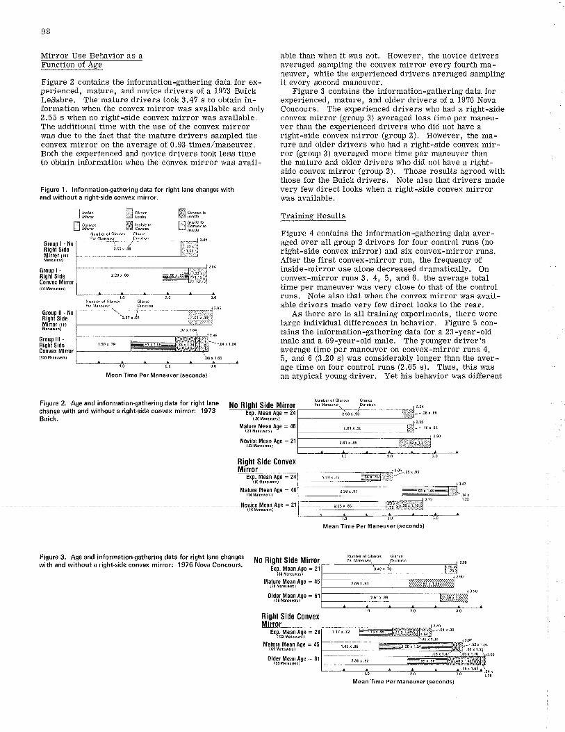
able than when it was not. However, the novice driversaveraged sampling the convex mirror every fourth ma-neuver, while the experienced drivers averaged sampling
98
Mirror Use Behavior as a@
perienced, mature, and novice drivers of a 19?3 BuickLeSabre. The mature drivers took 3.47 s to obtain in-
2,55 s when no right-side convex mirror was available.The additional time with the use of the convex mirrorwas due to the fact that the mature drivers sampled theconvex mirror on the average of 0,93 times/maneuver.
Figure 1. lnformation-gathering data for right lane changes withand w¡thout a r¡ght-side convex mirror,
Figure 3 contains the inÏormation-gathering data forexperienced, mature, and older drivers of a 1976 Nova
convex mirror (group 3) averaged less time per maneu-ver than the experienced drivers who did not have aright-side convex mirror (group 2), However, the ma-ture and older drivers who had a right-side convex mir-
formation when the convex mirror was available and only Concours, The e¡perienced drivers who had a right-side
Both the experienced and novice drivers took less time ror (group 3) averaged more time per maneuver thanto obtain information when the convex mirror was avail- the mature and older drivers who did not have a right-
side convex mirror (group 2). These results agreed withthose for the Buick drivers. Note also that drivers madevery few direct looks when a right-side convex mirrorwas available.
Training Results
Figure 4 contains the information-gathering data aver-aged over all group 2 drivers for four control runs (noright-side convex mirror) and six convex-mirror runs,After the first convex-mirror run, the frequency ofinside-mirror use alone decreased dramatically. Onconvex-mirror runs 3, 4, 5, and 6, the average totaltime per maneuver was very close to that of the controlruns. Note also that when the convex mirror was avail-able drivers made very few direct looks to the rear.
As there are in all training experiments, there werelarge individual differences in behavior. Figure 5 con-tains the information-gathering data for a 23-year-oldmale and a 69-year-old male, The younger driverrsaverage time per maneuver on convex-mirror runs 4,5, and 6 (3.20 s) was considerably longer than the aver-age time on four control runs (2.65 s). Thus, this wasan atypical young driver. Yet his behavior was different
f,ff co,,., roll¿t ,'s¡de
Group I - NoBioht SideMilrot trooMencuvers)
Group I -Riqhl SideConvex Mirror(11 flaneuvers)
Group ll - lloRiqhl SideMirror ttsmânewêrs)
Group lll -Right SideConver Mirrolf2¿0 tancuYë.s)
Figure 2. Age and information-gathering data for right lane NO Righl Side MirOlchange with and w¡thout a right-side convex mirror: 1973
-dp. ir=ean ÃSe=T¡
Buick. (36ten¿rveß)
Malüre Mean Aoe = 46(31 H¡n¿uvers) -
llovice Mean Aoe = 21{33tâncuv¿ß) -
Bight Side ConvexMinor
fl ¡¡s¡¿e
= coneer
= M¡trcr
71 or""'L-/l Looks
ffi ¡n"ø. rotiYi co¡ve¡
Glênce
2.54
.24 r.66
16x.93
2.90
Mean Time Per Maneuver (seconds)
206-.zst.ssExp. Mean Age = 24
{16 tan¿uveß)
Mature Mean Age = 46(14 tan€uveß)
(16 taneuve¡s
Figure 3. Age and informationgathering data for right lane chançswith and without a right-side convex mirror: 1976 Nova Concours.
No Righl Side MinorExp. Mean Age = 21
(36 tan!ù{eß)
Mature Mean Age = 45(28 flan€uY.ß)
older Mean Aoe = 61(28 Mån€uvs6 )-
Righl Side ConvexMirrol
Exo. Mean Aoe = 21'lrz¡ u¿n¿uveñ)
Mature Mean Aoe = 45(6f tsneuveßl -
0lder Mean Aoe = 61(56 tôneuv€ß) -
Mean Time Per Maneuver (seconds)
Mean T¡me Per Maneuver (seconds)
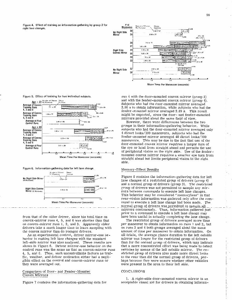
99
Figure 4. Effect of train¡ng on information gather¡ng by group 2 forright lane changes,
Figure 5. Effect of training for two individual subjects.
rge = za È'"',îT1,i,'"91-* .31,i:iAverage ol ConvexTraining Runs1,2and3Average ol ConvexTraining Runs4,5and6
Average ol FourConlrol Runs
Age = 69
Average ol ConvexTraininq Runs1,2and3Avemqe of Convexïraining Buns4,5and6
Average of FoulControl Runs
run 4 with the door-mounted convex mirror (group 3)and with the fender-mounted convex mirror (group 4).Subjects who had the door-mounted mirror averaged2.86 s to obtain information, while subjects who had thefender-mounted mirror averaged 2,89 s. This resultmight be expected, since the door- and fender-mountedmimors provided about the same field of view.
However, there were differences between the twogroups in their information-gathering behavior. Whilesubjects who had the door-mounted mirror averaged only4 direct tooks/100 maneuvers, subjects who had thefender-mounted mirror averaged 40 direct tooks/100maneuvers. This may be due to the fact that use of thedoor-mounted convex mirror requires a larger turn ofthe eye or head from straight ahead and permits the useof peripheral vision on the right side. Use of the fender-mounted convex mirror requires a smaller eye turn fromstraight ahead but limits peripheral vision to the rightside.
Memory-Effect Results
Figure I contains the information-gathering data for leftlane changes of a restricted group of drivers (group 4)and a normal group of drivers (group 3). The restrictedgroup of drivers was not permitted to sample any mir-rors between commands to execute left lane changes,This behavior may be considered "memorylesst' in thatrear-vision information was gathered only after the com-mand to execute a left lane change had been made, The
#olManeuvers
Glånce
l{o R¡ght SideM¡ilor
Riqht SideConvex Mirror
ilo B¡ght Side
M¡rror
.07 x,f.04 x 1.70
.08 ¡ 1,90.08 ¡.M
3.46
.06 x 1.383_15
1.88 r.83
l7
Figure 6. lnformat¡on-gather¡ng data for left lane change.
No Rioht Side Minor{68 tanãuversl
Right Side convexMittor tsg u"n'u',"r
from that of the older driver, since his total time onconvex-mimor runs 4, 5, and 6 was shorter than thaton convex-mirror runs 1, 2, and 3. Apparently olderdrivers take a much longer time to learn sampling withthe convex mirror than do younger drivers.
As an experimental control, driver mirror-use be-havior in making left lane changes with the standardleft-side mirror was also analyzed, These results areshown in Figure 6. Driver mirror-use behavior on thecontrol runs was the same as that on convex-mirror runs4, 5, and 6, Thus, such uncontrollable factors as traf-fic, weather, and driver motivation either had a negli-gible effect on the control and convex-mirror runs orthey were averaged out,
Comparison of Door- and Fender-Mounted
mirrors continuously, Thus, information gathered justprior to a command to execute a left lane change mayhave been useful in aetually completing the lane change.
The restricted group of drivers averaged more timeper maneuver to obtain information on runs 1 and 2, buton runs 3 and 4 both groups averaged about the sameamount of time per maneuver to obtain information. Onall trials, the average glance duration to the left outsidemirror was longer for the restricted group of driversthan for the normal group of drivers, which may indicatethat a more concentrated effort was being made to detectvehicles by means of the left outside mirror. The re-stricted group of drivers also made more direct looksto the rear than did the normal group of drivers, per-haps because they were unsure whether other vehicleswere present in the area to their left side.
CONCLUSIONS
1, A right-side door-mounted convex mirror is anacceptable visual aid for drivers in obtaining informa-
Mean T¡me Per Maneuver (seconds)
Figure 7 contains the information-gathering data for
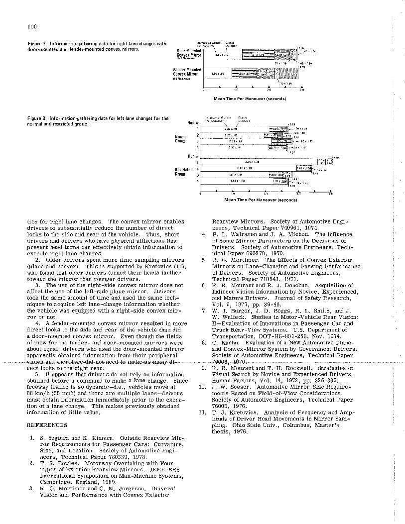
100
Figure 7. lnformat¡on-gathering data for right lane changes with |"iï,Y":,t9** 31,1i:."door-mounted and fender-mounted convex mirrors. Door M0unted
Convex Miror(240 tan!ure6l
Fender MountedConvex Mirror{92 taieuYe6l
Figure 8. lnformation-gathering data for left lane changes for thenormal and restricted group.
Mêan Time Per Mâneuver (seconds)
Num&r of Glan6 GlancsPer Mán¿uver Durâr¡ôn
l{ormalGroup
2.22 \ .95 F.ttt | .7142.23'.Ba FffiØâ:á
-.06 ¡ 1.21
l2 t 1.12
2.81
2.33 r.S 03 r 1.09
2.30 r.91 =.73x71
É.q ¡ l.l92.67
2.86 ¡ r.25 ÞrI-'¡
2.4s ¡ t.re E¡q'.s1.57t1.34 È.50t.o12'l',â
1.81 r 1.23 8.59 x
2.69
Mean Time Per Maneuver (sèconds)
5.
BestÌictedGroup
tion for right lane changes, The convex mirror enablesdrivers to substantially reduce the number of directlooks to the side and rear of the vehicle. Thus, shortdrivers and drivers who have physical afflictions thatprevent head turns can effectively obtain information toexecute right lane changes.
2. Older drivers spent more time sampling mirrors(plane and convex). This is supported by Kretovics (11),who found that older drivers turned their heads fartheTtoward the mirror than younger drivers.
3. The use of the right-side convex mirror does notaffect the use of the left-side plane mirror. Driverstook the same amount of time and used the same tech-niques to acquire left lane-change information whether
Rearview Mirrors. Society of Automotive Engi-neers, Technical Paper ?40961, I914.P. L. Walraven and J. A. Michon. The InfLuenceof Some Mirror Parameters on the Decisions ofDrivers. Society of Automotive Engineers, Tech-nical Paper 6902?0, 19?0.R. G. Mortimer. The Effects of Convex ExteriorMirrors on Lane-Changing and Passing Performanceof Drivers. Society of Automotive Engineers,Technical Paper 710543, 19?1.R. R. Mourant and R. J. Donohue. Acquisition ofIndirect Vision Information by Novice, Experienced,and Mature Drivers, Journal of Safety Research,Vol. 9, 19??, pp. 39-46.W. J. Burger, J. D. Beggs, R. L. Smith, and J.W. lVulfeck. Studies in Motor-Vehicle Rear Vision:Il-Evaluation of Innovations in Passenger Car andTruck Rear-View Systems. U.S. Department ofTransportation, DOT-HS-801-258, Nov. 1974.C. Kaehn. Evaluation of a New Automotive Plane-and Convex-Mirror System by Government Drivers,Society of Automotive Engineers, Technical Paper
4.
6.
the vehicle was equipped with a right-side convexror or not.
4. A fender-mounted convex mirror resulted in moredirect looks to the side and rear of the vehicle than dida door-mounted convex mirror. Even though the fieldsof view for the fender- and door-mounted mirrors wereabout equal, drivers who used the door-mounted mirrorapparently obtained information from their peripheral
rect looks to the right rear.5. It appears that drivers do not rely on information
obtained before a command to make a latre change. Sincefreeway traffic is so dynamic-i,e,, vehicles move at88 km/h (55 mph) and there are multiple laneslriversmust obtain information immediately prior to the execu-tion of a lane change. This makes previously obtainedinformation of little value.
REFERENCES
I. S. Sugiura and K. Kimura. Outside Rearview Mir-ror Requirements for Passenger Cars: Curvature,Size, and Location. Society of Automotive Engi-neers, Technical Paper 780339, 1978.
2. T. S. Bowles. Motorway Overtaking with FourTypes of Exterior Rearview Mirrors. IEEE-ERSInternational Symposium on Man-Machine Systems,Cambridge, England, 1969.
3. R. G. Mortimer and C, M. Jorgeson, DriversrVision and Performance with Convex Exterior
R. R. Mourant and T. H. Rockwell. Strategies ofVisual Search by Novice and Experienced Drivers.Human Factors, Vol. 14, 19?2, pp. 325-335.J. W. Seeser. Automotive Mirror Size Require-ments Based on Field-of-View Considerations.Society of Automotive Engineers, Technical Paper?6005, 1976.T. J. Kretovics. Analysis of Frequency and Amp-litude of Driver Head Movements in Mirror Sam-pling. Ohio State Univ., Columbus, Master'sthesis, 19?6.
t,
10.
11.
D is cu ssionThomas H. Rockwell, Department of Industrial and Sys-tems Engineering, Ohio State University, Columbus
The authors are to be commended for their approach tothis problem; indeed, the use of field studies for evalua-tion purposes is essential, albeit at some sacrifice ofexperimental control, Several of their experimentalfindings are consistent with my own work in mirror use,Glance durations are about right, although I would alsolike to see individual subject means and variances, sinceaggregation of the rate removes intrasubject and inter-subjeìt variation.
The paper is silent about the explicit instructionsgiven to the subject and about the effect of traffic on in-dividual maneuvers. I suspect that the velocity and den-sity of the following traffic in relation to the subjecilscar would influence glance frequency and duration, aswould the headways of automobiles directly ahead of thesubject driver. These variables are difficult to mea-sure, let alone control. I would like to have seen acomponents-of-variance analysis of key dependent mea-sures as they were affected by such independent variablesas lead-automobile headway, relative velocity andspacing of traffic following in the right lane, age, sex,and subject strategy.
The lack of sample sizes probably prohibited goodestimates of intersubject and intrasubject variation, al-though both of these give insights into the quality of ex-perimental control and interpretation of results.
The idea of using the left-side mirror sampling asan experimental control was an excellent one, partic-ularly for trip-duration effects and driver attentivenessand less so for traffic effects, The authors' concern thatperipheral vision may account for the sharp differencesin mirror sampling for the fender- versus door-mountedmirrors is probably valid (40/100 versus 4,/100 maneu-vers). I understand that the door-mounted position wasabout 800 from line of sight. Data from an Ohio State Univer-sity (OSU) study of 48 drivers (using their own cars infreeway lane changes and merges) that involved 7000mirror samples indicated that head turns cover 50 per-cent and eye movements 50 percent of the angle betweenline of sight and the mirror (11). A 40ô head turn in thiscase (to use the door-mounteã'-inirror) might have aI-lowed peripheral detection of target automobiles.
The OSU study also showed that age effects are sig-nificant in glance durations and head turns, but we foundolder drivers making greater head turns than youngerdrivers. (Older in this case was defined as over 45.)
101
As to the final judgment on convex mirrors, I be-lieve that this must wait until we ascertain the quality ofresultant maneuvers and can be assured of minimal ac-climation time. I presume from the paper that the ex-periments were not conducted in high-density trafficwith its attendant stress. This condition might be theultimate test of convex mirrors as aids to informationacquisition in driving.
Robert L. Henderson, National Highway Traffic SafetyAdministration
My remarks are directed, by request, at providing ad-ditional data on the general subject of convex mirrorsrather than diseussing the authors? paper,
I would like to describe briefly a National HighwayTraffic Safety Administration (NHTSA) contract I ammanaging that will eventually examine a rather largenumber of rearview mirror systems, It is being con-ducted for us by Bill Burger at Vector Research. Thebasic objective of the study is to evaluate driver mirror-use behavior while performing in-traffic maneuvers,The study uses a variety of mirror systems designed tomeet the requirements of a proposed new federal motorvehicle safety standard. Measures of mirror and directglance frequency and duration similar to those reportedby Mourant and Donohue will be the major criteria mea-sures, A repeated-measures design will be used inwhich the same 12 subjects will use all mirror systems.
Data collection on this main portion of the study isnow in progress. The data I will present today werecollected in the first phase of the study for the expresspurpose of selecting the radius of curvature for theconvex-mirror component of those systems that use con-vex mirrors.
The literature indicates that a 51-cm (20-in) radiusof curvature is probably the maximum usable convexitybecause of image minification and distortion. At theother extreme, when the radius exceeds about 203 cm(80 in), the limited gain in the field of view over a lessexpensive plane mirror does not justify the added cost.We have selected four specific values from within thisrange for this study-5L-cm, L02-cm (40-in), 140-cm(55-in), and 203-cm radii of curvature. Unlike somepast studies in which mirror size is held constant asconvexity varies, we held field of view constant for allconvexities by varying the size of the mirrors. The
patterns among older drivers, perhaps indicating lessconfidence in peripheral detection. We also found thatsex, driver height, and automobile size had little effecton left-side and inside mirror sampling.
The issue of memory probably is more importantwhen drivers overtake vehicles and refurn to the rightlane and may account for certain mirror sequence sam-p1ing. In that regard, were the differences in certaincombinations of mirror sampling found in group 3 (andin group 4) and not in group 1 the result of automobiletype or e4perience?
The authors are encouraged to plot glance frequencyagainst glance duration; i.e., do successive glances pro-duce shorter durations? Finally, we need to probe forthe driver's strategy in mirror use; i.e., does the driverdepend on the convex mirror for detection, evaluation,and decision information or does he or she use the con-vex mirror for detection and use other mirrors or di-rect looks and memory for the evaluation and decisionprocesses?
optimum convexity and, if there is, whether that optimumvalue varies as a function of the presence of other mir-rors in the system,
METHOD
Three vehicles were used; each vehicle had a mirrorsystem designed specifically to meet the requirementsof the proposed new mirror standard, The vehicleswere a passenger automobile, a light truck, and a van.Two Wpes of mirror systems were employed on the auto-mobile. The first type used two plane mirrors: one in-side and the other on the left outside. Each of thesemirrors was slightly larger than that found on passengerautomobiles today. The second type used a left outsideplane mirror somewhat larger than standard, a standardinside plane mirror, and a right outside convex mirror,The convex mirror (radius of curvature of 51, 102, 140,or 203 cm) was systematically varied.
The second type of automobile mirror system was
102
also used on the van and the pickup. In addition, thesetwo vehicles were tested with a combination plane andconvex mimor on each side and with a single convexmirror on each side. The convexity was again variedamong the four levels described earlier,
A semidynamic test condition was used to obtain dis-tance, speed, and gap-acceptance judgments. Subjectsviewed a target automobile approaching their own staticvehicles through the mirror system of interest, Eachof 12 subjects was tested by using each of 45 rearviewsystems properly counterbalanced in a repeated-measures design. These same 12 subjects will be usedlater in our on-the-road studies. A total of 11 BB0 trialswere run. Each subject has two blocks of eight speedand distance judgments and six lane-change judgmentsfor each mirror system. For all trials, subjects alsoperformed a forward tracking task for perceptual loading.
RESULTS
1. Learning: Significant learning effects were notedfor all mirror systems. Because of the counterbalancedorder of presentation, no clearcut and consistent learn-ing curves were noted for specific mirror systems, Inspite of the relatively large number of trials, it appearsthat learning is still taking place after approximately900 trials, indicating that learning to use convex mirrorsis a long-term phenomenon,
2. Relative distance error: Examination of the over-all relationship between convexity and overestimates orunderestimates of distance indicates some trends, butthe magnitude of the differences is so slight as to indi-cate no practical significance.
3. Absolute distance error: There was little dif-ference in average error as a function of mirror con-vexity. The same is true for the standard deviation.Although some of the differences were statistically sig-nificant, the practical differences are trivial,
4. Gap acceptance: We found small but fairly con-sistent trends toward better gap-acceptance performancefrom larger-radius mirrors. Best performance at allconvexities was found in mirror systems in which a planemirror was in close proximity to the convex mirror,
5. Subjective ratings: Perhaps the clearest and mostconsistent trends were found in the subjective ratings.Highly curved mirrors were consistenily judged to bemore difficult to learn and to produce less confideneethan less highly curved mirrors.
Rudolf G. Mortimer, Department of Health and SafetyEducation, University of Illinois at Urbana-Champaign
Historically, U.S. automobiles have been fitted withplane interior and exterior mirrors, The field of viewavailable from a plane mirror is determined by the sizeof the mirror and its distance from the eyes of thedriver. With respect to the exterior left-side mirror,the lateral field of view can be increased by increasingthe size of the mirror along its horizontal axis. Whilethere are some limitations on the extent to which themirror can be extended (due to limitations on the over-all width of motor vehicles), it is possible to obtain im-provements in the horizontal field of view to the left ofthe vehicle by improving the design location of the ex-terior left-side mimor and increasing its width. How-ever, this is not feasible with a plane mirror mountedon the right side of the vehicle, because of its muchgreater distance from the eyes of the driver.
A simple solution to increasing the field of view fromexterior mirrors is to use convex mirrors, Convexmirrors have been used by European and British driversfor years, mounted on the door or fender; a significantprecedent therefore exists to suggest that they can beused safely, However, U.S, manufacturers have notfelt that American drivers would willingly accept convexmirrors and have been concerned with the effects thatsuch mirrors can have on distance judgments becauseof the minification of objects,
To this end, a number of studies have been completedduring the last decade concerning the ability of driversto make various kinds of judgments related to the useof rearview mirrors in order to compare performancewith plane versus convex exterior mirrors. Thesestudies have used various types of measurements, suchas the frequency and duration of glances in interior andexterior mirrors (!!), detectability of vehicles in duskor dawn illumination (3), subjective evaluations of theeffects of headlight gla-re in rearview mirrors (3), dis-tance judgments (13), and gap-acceptance judgmlents(e-Ð.
As Mourant and Donohue have pointed out in theirpaper, the balance of these studies indicated that driversoverestimate the distance of a vehicle seen in a convexmirror, i.e., judge it to be further away than it reallyis, although, in a normal driving situation, when a driveralso has available the plane interior mirror, the judg-ments made when a convex exterior mirror or a planeexterior mirror were used were the same. Thus, itwould appear that drivers can make safe judgments withexterior convex mirrors, though their eye-fixation pat-
These data provide very little guidance for selectingthe convex-mirror component of the systems we are
are evident, in most instances the magnitude of the ob-served differences is so small as to håve little practicalsignificance. Consequently, we selected the convex-mirror components after considering the general litera-ture, the trends observed in our data, the extent of theobstruction to direct field of view, and judgments con-cerning what manufacturers might prefer for aestheticreasons or for overall standardization. For your in-formation, we are using 140-cm radius of curvature forthe right outside mirror for all systems that involveplane mirrors on the inside and left outside. For truckand van systems that use combination plane and convexmirrors on both sides of the vehicle, we are using 51-cm-radius convex mirrors. For the truck and van sys-tems that use a single convex mirror on each side, the102-cm radius of curvature was selected.
I appreciate the opportunity to describe this projectand hope that next year we will be able to report the re-sults of the on-the-road study.
terior mirror was used,The present study was concerned with eye-fixation
behavior of drivers who used plane and convex exteriormirrors mounted on the right side of the vehicle. Twolocations were selected for mounting of the mirror: onthe right door and on the right fender. Other variablesinvestigated were the effect of driver experience and age,effects of learning, and the effect of information obtainedfrom rearview mirrors shortly before the decision wasmade to execute a lane-change maneuver, which theauthors termed the memory effect.
The authors used a video recording technique to as-certain the frequency and duration of glances made bydrivers in lane-change maneuvers and measured the fre-quency and duration of glances in each of the rearviewmirrors. The emphasis in the study was on the compari-son of mirror use with and without a convex mirror onthe right side.
It is important to note one aspect of the instructionsgiven to the subjects. The subjects were told to use the
right-side convex mirror as a "go or no-go'r device.Furthermore, if a vehicle was noted in the convex mir-ror, the driver was to check its location by a directglance to the rear or by use of the inside mirror. Thus,any findings from this study will be limited because ofthe nature of the instructions given to the subjects abouthow they should use the convex right-side mirror'Clearly, the instructions were such that subjects werediscouraged from using the right-side convex mirrorto make estimates of distance or relative velocity of avehicle seen in the right lane before making a lanechange. One effect of this type of instruction wouldnaturally be to increase the proportion of direct glancesthe drivers would make when using a right-side convexmirror in relation to driving without it' Based on thedata presented (for example, in Figures 3 and 4 therewere relatively few direct looks to the rear when a con-vex mirror was used and there were relatively fewglances from the convex mirror to the inside mirror),it appears that there were few occasions when there wasa vehicle visible in the convex mirror at the time thata decision to make a right lane-change maneuver wasmade. There is no indication given in the paper as tothe proportion of maneuvers in which a vehicle was rea-sonably close to the subject's vehicle when the commandwas given to execute the maneuver, either when theright-side mirrors were in use or without them. Itwould seem that this could have been an important pieceof data that should have been available from the videorecordings and might have been taken into account ino<plaining some of the findings.
I was somewhat concerned that there were relativelyfew subjects used in some of the conditions. For ex-ample, the findings in Figure 2 are based on the resultof only three subjects in each of the age and experiencegroups, So few subjects would scarcely be enough toallow reasonable differences to be discovered betweencategories of this variable.
However, it was refreshing to see the findings inFigure 6, which indicated that, when mirror-use be-havior was observed in left lane changing for the fivesubjects in group 2, the performance in left lane-changemaneuvers was very similar when the vehicle wasequipped with a right-side convex mirror and on a setof control runs when it was without the right-side mir-ror. This indicates that the overall procedure appearsto have a good degree of reliability, at least when 60
or more maneuvers are involved.The authors also address the effect of the age of the
drivers. In this case, there were substantially morein the two 2 and 3) that
were used for this comparison, whichperienced drivers required less time to obtain mirrorinformation than mature and older drivers when a right-side convex mirror was available, whereas without theright-side convex mirror aII three groups required ap-proximately the same amount of mirror information-gathering time.
A comparison is also shown, in Figure ?, betweendoor- and fender-mounted right-side convex-mirror per-formance, This figure appeared to be based on the com-parison of the performance of the 12 subjects in group3 and the 11 subjects in group 4 who had a mean time toobtain rear-vision information of 2,86 s and 2.9 s, re-spectively, for the door-mounted and fender-mountedconvex mirror. It appeared to me, however, that thiscomparison was confounded by differences between thesetwo groups. Group 3 was described as carrying out theexperiment in the normal mode of mirror scanning,whereas group 4 was restricted in scanning behavior;i,e,, the subjects were not permitted to scan the mir-rors until the command had been given by the experi-
103
menter to begin a lane-change maneuver' The purposewas to permit evaluation of the memory effect' It seemsto me that these two groups should not be used to com-pare another variable. The effect of fender mountingversus door mounting of the convex mirror could per-haps be obtained from the data obtained on group 1, whichcarried out the normal task with a fender-mounted con-vex mirror on the right side, compared with group 3,which performed the task with the convex mirror mountedon the right door, In that comparison, the mean timeto obtain information was 2.84 and 2'86 s for the fender-and door -mounted convex mirrors, respectively.
The concept of eva-luating the memory effect is cer-tainly an interesting one and shows that the authors weresensitive to many subtle variables that could affectdriver behavior with rearview mirrors. This effect wasevaluated by comparing a group operating in the normalmode with a group operating in the restricted mode inmaling left lane-change maneuvers. While theinformation-gathering time was substantially longer onthe first two (out of four) trials in the restricted group,indicating a potential memory effect, there were no dif-ferences in the subsequent two trials. While this mightindicate that the memory effect had been erased by thethird and fourth trials, I feel that this is not likely. Isit possible, for example, that a motivational effect wasoperating, due to a slightly greater stress imposed onthe subjects and the interaction with the experimenter,who called out the command to begin the lane-changemaneuver?
Based on the viewing behavior that was measured inthis study, it does seem reasonable that convex mirrorscould be used on the right side of the vehicle. The totalamount of time spent viewing mirrors was not increasedsignificantly by the addition of this third mirror on theright side. Certainly, a convex right-side mirror ofadequate size and moderate radius of curvature, suchas that used in these studies, would greatly improve thefield of view to the right of the vehicle, where the pres-ent use of a plane mirror or no mirror at all providesa potentially hazardous blind spot'
Although this study indicated that the fender-mountedconvex mirror resulted in more direct looks to the sideand rear of the vehicle than did a door-mounted convexmirror, this should not be taken to imply that a fender-mounted location is undesirable, Location on the fenderhas some additional advantages, such as actually pro-viding a greater field of view to the right' This is par-ticularly valuable in dense traffic when another vehicleis close by on the right side and potentially outside thefield of view of a door-mounted mirror but visible in atencter-molrnted mrrror. Èieconcuyt a renqer-mounleomirror requires less divergence of the eyes from theforward field of view, which is the most important Io-cation to be scanned by the driver in normal drivingsituations.
This study has been useful in taking a look at age andmaturational factors. Certainly, more data of this typewould be valuable.
In this context, the authors have studied the memoryeffect, which was of considerable interest and requiresfurther study. The memory effect could be particularlyimportant in those emergency situations where there islittle time to obtain additional visual information and arapid decision must be made as to the most appropriateevasive maneuver to make. In such casesr there maybe little or no time for adequate mirror scanning to de-termine the locations of other potential vehicles, and thememory effect could be of critical importance. Eyefixations of e¡perienced drivers indicate that they scanthe environment all around the vehicle frequently; it maybe premature to suggest that drivers do not retain an
104
appraisal of the location of other vehicles around themin short-term memory,
FinaIIy, one might legitimatety ask what the relevanceof obtaining frequency and duration of glance behaviorin mirrors is in relationship to accidents in which rear-vision information may have been inadequate? The over-all duration of mirror glances would be important inthose situations where little time is available to makea decision in an evasive maneuver, On the other hand,the quality of the information that is obtained is alsocritical. Thus, one might ask whether drivers obtainmore accurate information concerning the location, dis-tance, and relative velocity of other vehicles with aright-side convex mirror than with no mirror on theright side and how safe the resulting lane-change maneu-vers are, The latter question was not addressed in thisstudy, This raises the issue of the relevance of per-formance criteria in rear-visibility sfudies. perhapssuch criteria carurot be structured properly until moreinformation becomes available as to the underlyingcauses of crashes that involve inadequacies in visibilityto the rear.
REFERENCES
12. C. R. Kelley and D. J. Prosin; Dunlap and Associ-ates, Inc. Motor Vehicle Rear Vision. NationalHighway Safety Bureau, U.S. Department of Trans-portation, 1969.
13. G. E. Rowland, C. A. Silver, S. C. Volinsþ, J.S. Behrman, N. F. Nichols, and W. Clishman. AComparison of Plane and Convex Rear-View Mir-rors for Passenger Automobiles. National HighwayTraffic Safety Administration, U.S. Department ofTransportation, 19?0,
Authors'ClosureBoth Mortimer and Rockwell had positive comments on
the use of left lane-change data for experimental controlpurposes. These left lane-change data indicated thatthe effects of traffic, weather, and driver motivationwere averaged out when computed over 60 left lane-change maneuvers, These data may also serve as astandard reference when considering driver searchbehavior with reference to left lane changes. In thisregard, the data show that drivers made only six directlooks to the rear while executing 12? left lane-changemaneuvers. However, drivers did rely heavily on theirleft outside mirrors; they looked at them more than twiceper maneuver,
Concerns were voiced about the small number of sub-jects in the study of age effects. We agree that moredata should be collected on this very important variable.The data could be used to develop aids and countermea-sures for the older driver. Perhaps older drivers willfind convex mirrors useful, in that they will partiallyeliminate the need for head turns to the right rear.
It should be noted that all data were collected whiledriving on freeways in the city of Detroit in moderateto heavy traffic. We considered this to be a very de-manding task for most drivers, Thus, instructions tothe zubjects probably had very little effect on driverperformance, Many times, when the experimenter gavethe command to execute a lane change, other traffic inadjacent lanes prevented the subject from immediatelyexecuting the maneuver, Thus drivers had to search byusing their mirrors or by making direct looks to deter-mine when to proceed with the lane change. Because thetraffic flow on the freeways was always moderate toheavy, it had little effect on comparisons between door-and fender-mounted mirrors,
Since the data in this study have shown that the useof a door-mounted convex mirror has reduced the fre-quency of direct looks per 100 maneuvers from 40 (withno right-side mirror) to 4, we believe that automobiledrivers will have no problem in using a right-side con-vex mirror.
Publication of this paper sponsored by Committee on Visibility.
HumanIn-Vehicle Route GuidanceCon¡a,{ L. Dudek, Te:<as Transportation Institute, Te¡¡as A&M University,
College Station
This paper considers füe development and mâintenance of credibilityin the design, implementation, and operation of a route guidance syi-tem. Because drivers will have positive att¡tudes about a system thatprovides them with relevant, reliable, and accurate informãtion, allprecaut¡ons must be taken to ensure that these driver expectations aremet. Mæsages must be presented clearly and must allow ample timefor the driver to respond to a given s¡tuation, Factors thãt a¡fectreading time of displays include driver work load, message load, mes-sage length, message familiarity, and display format. ln order to main-tain driver credibility, surveillance must be an integral part of a routeguidance system. Such surveillance must be able tõ deiect adversecondit¡ons, val¡date the adverse condit¡ons, and determine the natureand scope of the problem. Electronic sensor surveillance, however, hassome limitations. Because it is a blind system, (a) some form of visual
validation and assessment of incidents to ensure the accuracy of dis-played messages and (b) some guarantee of adequate system mainte-nanoe are necessary. A "forgiving" system--one that alerts the dr¡verand provides instuct¡ons about how to rcturn to a scheduled routeafter a d¡version-must also be considered.
An important consideration in a successful routeguidance system for the United States (where successis measured by achieving desirable driver response) isto develop and maintain credibility, that is, driver faittrin the system. The quickest way to fail is to lose driverconfidence. The most elaborate and costliest system can
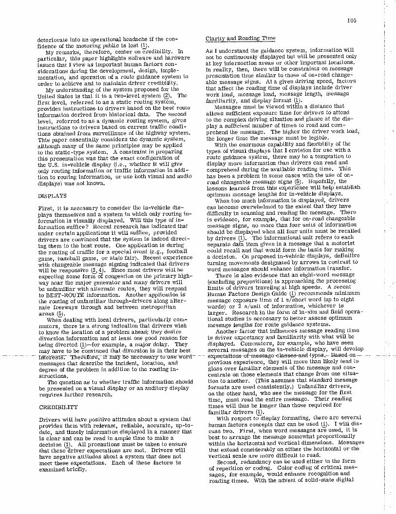
deteriorate into an operational headache if the con-fidence of the motoring public is lost Q.
My remarks, therefore, center on credibility. Inparticular, this paper highlights software and hardwareissues that I view as important human factors con-sideratio¡rs during the development, design, imple-mentation, and operation of a route guidance system inorder to achieve and to maintain driver credibility.
My understanding of the system proposed for theUnited States is that it is a two-level system (þ. Thefirst level, referred to as a static routing system'provides instructions to drivers based on the best routeinformation derived from historical data. The secondlevel, referred to as a dynamic routing system, givesinstructions to drivers based on curent traffic condi-tions obt¿ined from surveillance of the highway system.This paper essentially considers the dynamic system,although many of the same principles may be appliedto the static-type system. A constraint in preparingthis presentation was that the exact configuration ofthe U.S. in-vehicle display (i.e., whether it will giveonly routing information or traffic information in addi-tion to routing information, or use both visual and audiodisplays) was not known.
DISPLAYS
First, it is necessary to consider the in-vehicle dis-plays themselves and a system in which only routing in-iormation is visually displayed. Will this type of in-formation suffice? Recent research has índicated thatunder certain applications it will suffice, provideddrivers are convinced that the system is indeed direct-ing them to the best route. One application Ís duringthe routing of traffic for a special event (e.g., footballgame, baseball game, or state fair). Recent ex¡leriencewith changeable message signing indicated that driverswill be responsive p, !). Since most drivers will bee4pecting sbme form- oT congestion on the primary high-\¡/ay near the major generator and many drivers rvillbe unfamiliar with alternate routes, they will respondto BEST-ROUTE information. Another apptication isthe routing of unfamitiar through-drivers along alter-nate freeways through and between metropolitanareas þ.
When dealing with local drivers, particul;arly com-muters, there is a strong indication that drivers wishto know the location of a problem ahead; they desirediversion inJormation and at least one good reason forbeíng diverted (!)-for example, a major delay. Theymay have to be convinced that diversion is in their best
105
Clarity and Reading fime
As I understand the guidance system, information willnot be continuously displayed but will be presented onlyat key intersection areas or other important locations.In reality, then, there will be constraints on messagepresentation time similar to those of on-road change-able message signs. At a given driving speed, factorsthat affect the reading time of displays include driverwork load, message load, message length, messagefamiliarity, and disptay format [).
Messages must be viewed within a distance thatallows sufficient exposure tíme for drivers to attendto the complex driving situation and gliance at the dis-play a sufficient number of times to read and com-þrehend the message. The higher the driver work load,the longer time the message must be legibie.
With the enormous capability and flexibility of thetypes of visual displays that I envision for use with aroute guidance system, there may be a temptation todisplay more information ttran drivers can read a¡dcomprehend during the available reading time. Thishas þeen a problem in some cases
"¡¡ith the use of on-
road clrangeable message signs þJ. Hopetully' thelessons learned from this ex¡leriãnce will help establishoptimum message lengths for in-vehicle displays.
When too much information is displayed, driverscan become overwhelmed to the extent that they havedifficutty in scaruring and reading the message. Thereis evidence, for erømple, that for on-road changeab-Iemessage signs, no more than four units of informationshould be displayed when all four units must be recalledbv drívers (1). The informational unit refers to eachsäparate daã item given in a message tl¡at a motoristcould recall and that would form the basis for makinga decision. On proposed in-vehicle displays, definitiveturning movements designated by arrows in contrast toword messages shorld enlrance ir¡formation transfer.
There is also evidence that an eight-word message(excluding prepositions) is approaching the processinglimits of drivers traveling at high speeds. A recentHuman Factors Design Guide (! recommends minimummessage exposure time of 1 s,/short word (up to eightwords) or 2 s/unit of information, whichever isIarger. Research in the form of in-situ and field opera-tional studies is necessary to better assess optimummessage lengths for route guidance systems.
Another factor ttrat influences message reading timeis driver ex¡lectancy and familiarity with what will be
displayed. Commuters, for enample, who have seensevèral messages on the in-vehicle display, will develop
messages that describe the incident, location, anddegree of the problem in addition to the routing in-structions.
The question as to whether trafTic information shouldbe presented on a visual display or an auditory dispÞyrequires further research.
CREDIBILITY
Drivers will have positive attitudes about a system thatprovides them with relevant, reliable, accurate, up-to-date, and timely information displayed in a manner thatis clear and can be read in ample tíme to make adecision (Ð. Atl precautions must be taken to ensurethat theseãriver expectations are met. Drivers willhave negative attitudes abqrt a system that does notmeet these e4pectations. Each of these factors ise:ra,mined briefly.
prèvious ex¡rerience, they will more than likely tend to
þloss over familiar elements of the message and con-õentrate on those elements that change from one situa-tion to another. (This assumes that standard messageformats are used consistently.) Unfamiliar drivers,on the other hand, who see the message for the firsttime, must read the entire message. Their readÍngtime's will thus be longer than those required forfamiliar drivers [).
With respect tildisplay formating, there are severalhuman factors concepts that can be used Q. I will dis-cuss two. First, when word messages are used, it isbest to arrange the message somewlrat proportionallywithin the horizontal and vertical dimensions. Messagesthat extend considerably on either the horizontal or thevertical scale are more difficult to read.
Second, redundancy can be used either in the formof repetition or coding. Color coding of critical mes-sages, for example, would enhance recognition andreã¿i¡ig times. With the advent of solid-state digital

106
television image generation and anticipated technologyadvances in the future, this is not outside the realmifreality.
There are various messages Ûrat can be used todescribe traffic conditions or so-called traffic states.Recent studies have indicated that drivers can onlydistinguish about three, or at most four, levels oftra-ffic conditions (Q). The studies have also shown Û¡,atdrivers from small cities perceive congestion at amuch lower traffic density than drivers from largecities. 'lüords used to describe traffic conditions mustbe carefully selected, For example, the descriptorsSTOP AND GO TRAFFIC and NORMAL TRAFFIC arevery vague and should not be used. The traffic statedescriptor, CONGESTION, is vague and should not beused [).
Drivers who are given delay durations (or timesaved) will base their decisions to divert or to continueon the delay information more than informationabout the particular type of incident. If a quantitativeindication of delay (in minutes) is displayed, it must bereasonably accurate because its vatidity can be easilychecked by the drivers. Studies conducted in four U.S.cities revealed that more than 50 percent of the sur-veyed drivers indicated that they would divert to avoida delay of 20 min or more. OnIy B percent stated thatthey would divert to a delay duration of less than 5 min(!). MAJOR ACCIDENT implies to the average drivera deÞy of at least 20-2ã min and MINOR ACCIDENT,a delay of not more than 15 min Q.In areas where most drivers are primarily com-muters, cross-street names should be used to identifythe location of the incident. The incident location mayalso be referenced to a well-known landmark if avail-able. For unfamiliar drivers, the incident locationshould be e4pressed in terms of distance (1). Whennames of cities are used on the display, thãy shouldbe identical to those used on existing static signs [).Even with the flexibility of the in-vehicle disptafs,it will be necessary in many cases to use abbrevia-tÍons because of the physical size limitations. Driverinterpretations of several types of abbreviations morecommonly used with tra-ffic condition and routing infor-mation are not fully known at this time (5). More re-search is needed in order to ensure that-proper, well-understood abbreviations are used.
Timely Intormation
Routing and lane assignment information must be givenin ample time for drivers to respond to instructioñs.
to the static signs is important. It is yet to be deter-mined if routing instructions should be displayed inadvance of interchange signs, in coqjunction withadvance interchange signs, or beyond advance inter-change signs.
Relevant Information
Telling drivers that they are in congested traffic orrepeatedly telling commuters of recurrent congestionwhen such information is obvious decreases confidencein the capability of the system to provide useful in-for-mation. What is obvious should never be dispÞyed e.The route guidance system should not be used to -balance demands with availabte capacity during recur-rent congestion conditions, There have been attemptsto balance on-ramp demands during daily peak periõdsby suggesting that drivers use other ramps on the free-way, This approach was found to be ineffective and isa good way to lose credibility, Drivers are concernedwith their individual travel times and are unconcernedwith optimizing flow in a corridor. It is importantthat they realize a significant reduction in their personaltravel time if they are to continuously abide by the in-formation presented Q.Reliable and Accurate Information
The specific messages that can be displayed with con-fidence to maintain driver credibility are influenced bythe operating agency's ability to detect a tra-ffic problemand to determine the nature and scope of the problem.Therefore, surveillance will be an integral part of aroute guidance system and must serve the followingfunctions þ:
1. Detection of adverse conditions,2. Validation of the adverse conditions, and3. Determination of the nature and scope of the
problem.
Knowing what is occurring on the affected freewaysand streets has an impact on tlre messages one can dis-play. Driver credibility is at stale. Repeated displayof erroneous information or route recommendationsthat are not the best in the driver's viewpoint are waysof losing driver confidence.
Electronic surveillance with in-place detectors doesnot always ensure that the information received isaccurate. Detection systems seem to be a problem inseveral existing changeable message sign installations.
l-
turning point and far enough upstream of any possibletra-ffic queues so tÌ¡at drivers can maneuver into theappropriate lane. Therefore, a route guidance systemmust have the capability for measuring traffic queuesand adjusting itself accordingly so ürat drivers are nottrapped. For example, under light flow conditíons,the lane assignment in-formation can be made ratheiclose to the turning point; but, under heavy 1¡rffic con-ditions, it must be made much sooner.
We also need to consider those cases where thedriver has two choice points in close proximity. Thesituation at a freeway-to-freeway interchange is anenample. Information may have to be given far inadvance of the interchange. If so, it must be presentedclearly so that the driver does not incorrecily exit at aramp upstream of the major interchange. It may benec-e,ss€.ry, therefore,, to disptay route shields e.Without question, the in-formation displayed m-ust becompatible wÍtlt existing static guide signs. Therefore,the relative time frame or spatial frame with respect
Iimitations. First, there could be considerable delayin recognizing that an incident has occurred (S. Thisis due to several reasons:
1. Because of cost, sensors are normally placed atlong intervals-0.8 km (0.5 mile) or longer on freeways.
2. Sensors are a point source of information.3. Current incident detection algorithms are not
100 percent accurate. (Changing the atgorithm parame-ters to inòrease the percentage of incidents detectedalso increases the chance of false alarms. Thus, thereis a need for additional work in this area.)
Another limitation of electronic sensor surveilLanceis that it is a blind system. The agency must rely onother means to assess the nature of the incident inorder to display appropriate messages.
Because electronic surveillance is a blind system,some form of visual validation and assessment of inci-dents is necessary to ensure that accurate messages
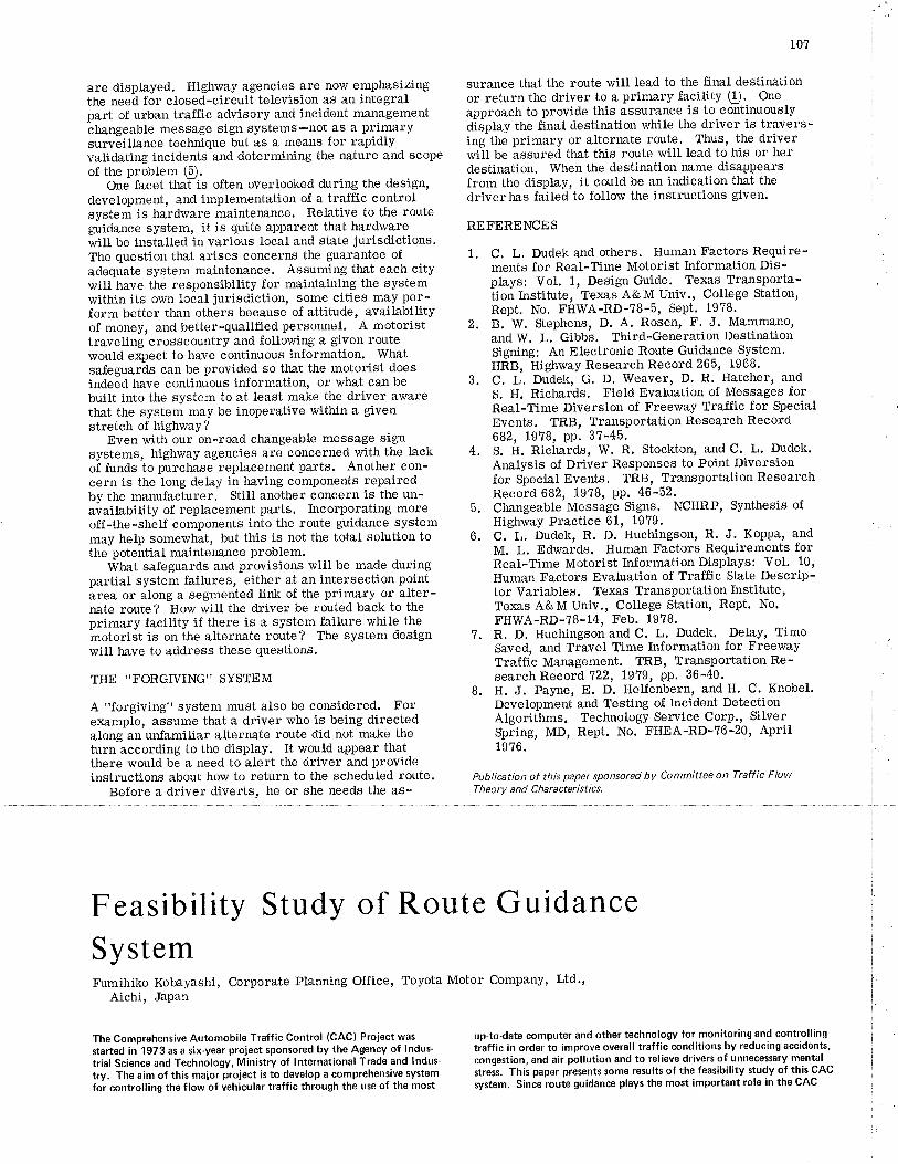
are displayed. Highway agencies are now emphasizingthe need for closed-circuit television as an integralpart of urban traffic advisory and incident managementchangeable message sign systems-not as a primarysurveillance technique but as a means for rapidlyvalidating incidents and determining the nature and scopeof the problem (Q.
One facet thafis often overlooked during the design,development, and implementation of a tra^ffic controlsystem is hardware maintenance. Relative to the routeguidance system, it is quite apparent that hardwarewill be installed in various local and state jurisdictions.The question that arises concerfft the guarantee ofadequate system maintenance. Assuming that each citywill have the responsibility for maintaining the systemwithin its own local jurisdictíon, some cities may per-form better than others because of attitude, availabilityof money, and better-qualified persormel. A motoristtraveling crosscountry and following a given routewould e>çect to have continuous information. Whatsafeguards can be provided so that the motorist doesindeed have continuous information, or what can bebuilt into the system to at least make the driver awarethat the system may be inoperative within a givenstretch of highwaY?
Even with our on-road changeable message signsystems, highway agencies are concerned with the lackof funds to purchase replacement parts. Another con-cern is the long detay in having components repairedby the manufacturer. Stitl another concern is the un-availabitity of replacement parts. Incorporating moreoff-the-shelf components into the route guidance systemmay help somewhat, but this is not the total solution tothe potential mainte¡rance problem.
What safeguards and provisions will be made duringpartial system failures, either at an intersection pointarea or along a segmented link of the primary or alter-nate route? How will the driver be routed back to theprimary facility if there is a system failure while themotorist is on the alternate route? The system designwill have to address these questions.
THE''FORGTVING'' SYSTEM
A "forgiving" system must also be considered. Forexample, assume that a driver who is being directedalong an unfamiliar alternate route did not make theturn according to the display. It would appear thatthere would be a need to alert the driver and provideinstructions about how to return to the scheduled route.
Before a driver diverts, he or she needs the as-
107
sura¡ce that the route will lead to the final destinationor return the driver to a primary facility Q. O¡¡e
approach to provide this assurance is to continuouslydisplay the final destination while the driver is travers-ing the primary or alternate route. Thus, the driverwill be assured that this route will lead to his or herdestination. When the destir¡ation name disappearsfrom the display, it could be an indication that thedriverhas failed to follow the instructions gven'
REFERENCES
1. C. L. Dudek and others. Human Factors Require-ments for Real-fime Motorist Information Dis-plays: Vol. 1, Design Guide. Texas Transporta-tion Institute, Texas A& M Univ., College Station,Rept. No. FHWA-RD-?8-5, Sept. 1978.
2. B. W. Stepherc, D. A. Rosen, F. J. Mammanotand W. L. Gibbs. Third-Generation DestinationSigning: An Etectronic Route Guidance System.HRB, Highway Research Record 265, 1968.
3. C. L. Dudek, G. D, Weaver, D. R. Hatcher, andS. H. Richards. Field Evaluation of Messages forReal-Time Diversion of Freeway TrafÏic for SpecialEvents. TRB, Transportation Research Record682, 19?8, pp. 3?-45.
4. S. H. Richards, W. R. Stockton, and C. L. Dudek.Analysis of Driver Responses to Point Diversionfor SpecÍal Events. TRB, Transportation ResearchRecord 682, 1978, PP. 46-52.
5. Changeable-Message Signs. NCHRP' Synthesis ofHighway Practice 61, 19?9.
6. C. L. Dudek, R. D. Huchingson, R. J. Koppa, andM. L. Edwards. Human Factors Requirements forReal-Time Motoríst l¡formation Displays: VoI. 10,
Human Factors Evaluation of Traffic State Descrip-tor Variables. Texas Transportation Institute,Texas A&M Univ., College Station, Rept. No.FHWA-RD-78-14, Feb. 1978.
1. R. D. HuchingsonandC. L. Dudek. DeLay, TimeSaved, and Travel Tlme Information for FreewayTra-ffic Management. TRB, Transportation Re-search Record 722, l9'l9t PP. 36-40.
B. H. J. Payne, E. D. Helfenbern, and H. C. Knobel.Development and Testing of Incident DetectionAlgorithms. Technotogy Service Corp., SilverSpring, MD, Rept. No. FHEA-RD-?6-20, April1976.
Pubtication of this paper sponsored by Committee on Traffic FlowT heo ry a nd C ha racter i st ics.
Feasibility Study of Route GuidanceSystemFumihiko Kobayashi, Corporate Planning Office, Toyota Motor Company,
Aichi, JaPan
The Comprehensive Automobile Traffic Control (CAC) Proiect was
started in 1973 as a six-year project sponsored by the Agency of lndus-trial Science and Technology, Ministry of lnternational Trade and lndus'try. The aim of this major project is to develop a comprehensive system
for controlling the flow of vehicular traffic through the use of the most
up-todate computer and other technology for monitoring and controllingtraffic in order to improve overall traffic condit¡ons by reducing accidents,
congestion, and air pollution and to relieve drivers of unnecessary mentalstress. This paper presents some results of the feasib¡lity study of this CAC
system. Since route guidance plays the most important role in the CAC
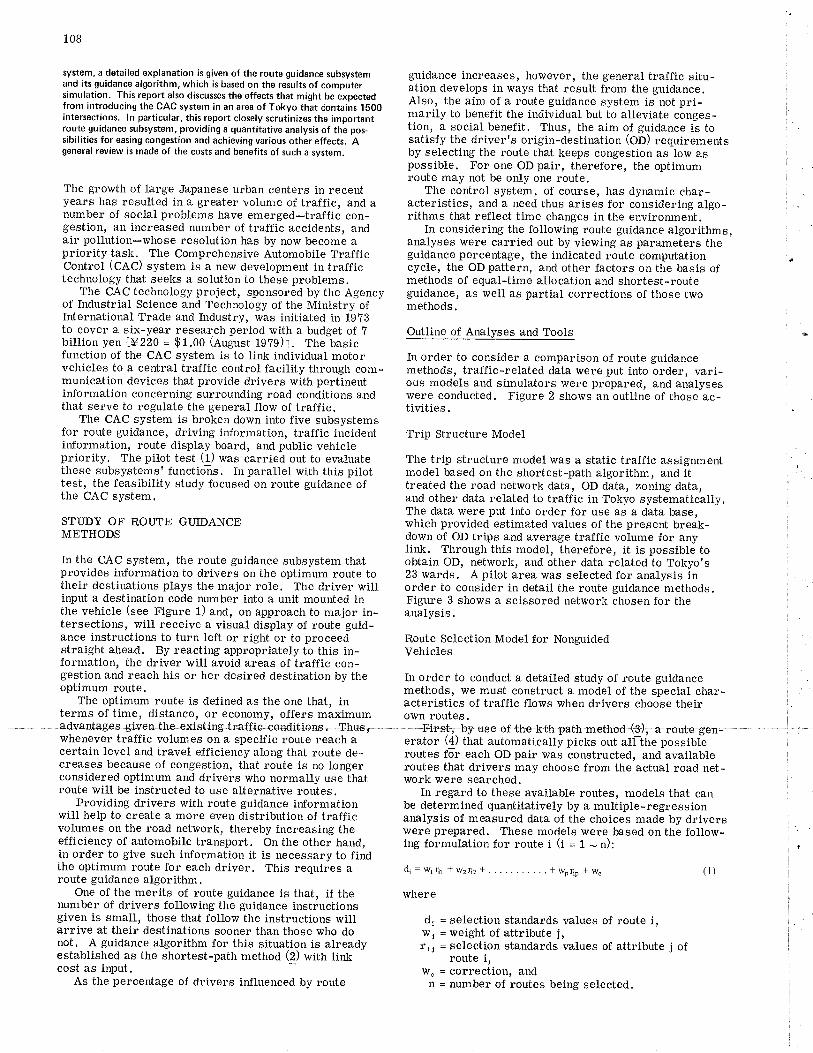
108
system, a detailed explanation is given of the route guidance subsystemand its guidance algorithm, which is based on the results of computersimulation. This report also discusses the effects that might be expectedfrom introducing the CAC system in an area of Tokyo that contains 1boointersections. ln particular, this report closely scrutinizes the importantroute gu¡danc€ subsystem, providing a quantitative analysis of the pos-sibilities for easing congestion and achieving var¡ous other effects. Açneral review is made of the costs and benefits of such a system.
The growth of large Japanese urban centers in recentyears has resulted in a greater volume of traffic, and anumber of social problems have emerged-traffic con-gestion, an increased number of traffic accidents, andair pollution-r,vhose resolution has by now become apriority task. The Comprehensive Automobile TrafficControl (CAC) system is a new development in traffictechnology that seeks a solution to these problems.
The CAC technology project, sponsored by the Agencyof Industrial Science and Technology of the Ministry ofInternational Trade and Industry, was initiated in 1973to cover a six-year research period with a budget of 7billion yen [#220 = $f .OO (August 19?9)]. The basicfunction of the CAC system is to link individual motorvehicles to a central traffic control facility through com-munication devices that provide drivers with pertinentinformation concerning surrounding road conditions andthat serve to regulate the general flow of traffic.
The CAC system is broken down into five subsystemsfor route guidance, driving information, traffic incidentinformation, route display board, and public vehiclepriority. The pilot test (1) was carried out to evaluatethese subsystemst functions. In parallel with this pitottest, the feasibility study focused on route guidance ofthe CAC system.
STUDY OF ROUTE GUIDANCEMETHODS
In the CAC system, the route guidance subsystem thatprovides information to drivers on the optimum route totheir destinations plays the major role. The driver willinput a destination code number into a unit mounted inthe vehicle (see Figure 1) and, on approach to major in-tersections, will receive a visual display of route guid-ance instructions to turn left or right or to proceedstraight ahead. By reacting appropriately to this in-formation, the driver will avoid areas of traffie con-gestion and reach his or her desired destination by theoptimum route.
The optimum route is defined as the one that, interms of time, distance, or economy, offers maximum
guidance increases, however, the general traffic situ-ation develops in ways that result from the guidance.Also, the aÌm of a route guidance system is not pri-marily to benefit the individual but to alleviate conges-tion, a social benefit. Thus, the aim of guidance is tosatisfy the driverts origin-destination (OO) requirementsby selecting the route that keeps congestion as low aspossible. For one ODpair, therefore, the optimumroute may not be only one route.
The control system, of course, has dynamic char-acteristics, and a need thus arises for considering algo-rithms that reflect time changes in the environment.
In considering the following route guidance algorithms,analyses were carried out by viewing as parameters theguidance percentage, the indicated route computationcycle, the OD pattern, and other factors on the basis ofmethods of equal-time allocation and shortest-routeguidance, as well as partial corrections of those tu/omethods.
Outline of Analyses and Tools
In order to consider a comparison of route guidancemethods, traffic-related data were put into order, vari-ous models and simulators were prepared, and analyseswere conducted. Figure 2 shows an outline of those ac-tivities.
Trip Structure Model
the trip structure model rvas a static traffic assignmentmodel based on the shortest-path algorithm, and ittreated the road network data, OD data, zoning data,and other data related to traffic in Tokyo systematically.The data were put into order for use as a data base,which provided estimated values of the present break-down of OD trips and average traffic volume for anylink. Through this model, therefore, it is possible toobtain OD, network, and other data related to Tokyo's23 wards. A pilot area was selected for analysis inorder to consider in detail the route guidance methods.Figure 3 shows a scissored network chosen for theanalysis.
Route Selection Model for. NonguidedVehicles
In order to conduct a detailed study of route guidancemethods, we must construct a model of the special char-acteristics of traffic flows when drivers choose theirown routes.
whenever traffic volumes on a specific route reach acertain level and travel efficiency along that route de-creases because of congestion, that route is no longerconsidered optimum and drivers who normally use thatroute will be instructed to use alternative routes,
Providing drivers with route guidance informationwill help to create a more even distribution of trafficvolumes on the road network, thereby increasing theefficiency of automobile transport. On the other hand,in order to give such information it is necessary to findthe optimum route for each driver. This requires aroute guidance algorithm.
One of the merits of route guidance is that, if thenumber of drivers following the guidance instructionsgiven is small, those that follow the instructions willarrive at their destinations sooner than those who donot. A guidance algorithm for this situation is alreadyestablished as the shortest-path method (2) with linkcost as input.
As the percentage of drivers influenced by route
¡r!¡¡ lr4!¡¡ \u/, 4 ¡vutg Éçt¡-erator (¿) ttrat automatically picks out ali-tÍre possiblèroutes for each OD pair was constructed, and availableroutes that drivers may choose from the actual road net-\Àrork were searched.
In regard to these available routes, models that canbe determined quantitatively by a multiple-regressionanalysis of measured data of the choices made by driverswere prepared. These models were based on the follorv-ing formulation for route i (i = t - n):
di=wrru *wzr¡z'l ....*wo¡io*w" (l)
where
dr = selection standards values of route i,wr = weight of attribute i,rr¡ = sêI€ction standards values of attribute j of
route i,\¡/c = Corre.tiOn, andn = number of routes being selected.
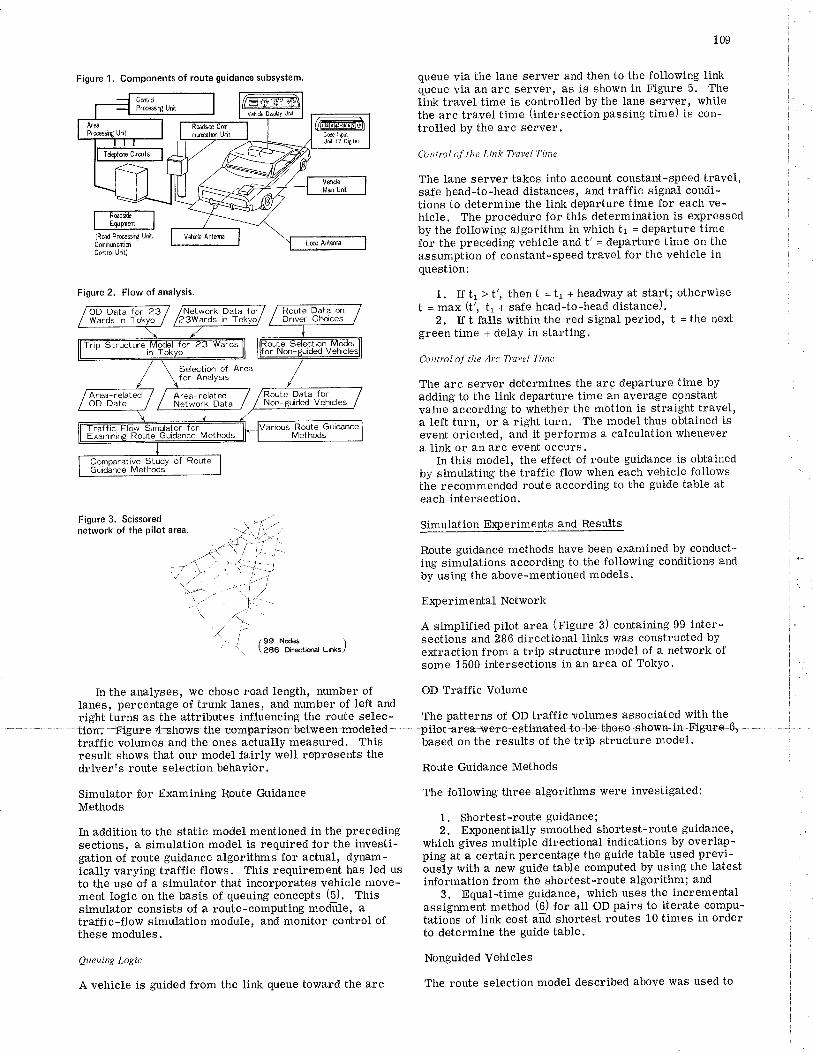
Figure 1. Components of route guidance subsystem'
Figure 3. Scissorednetwork of the pilot area.
In the analyses, we chose road length, number oflanes, percentage of trunk lanes, and number of left andright turns as the attributes inJluencing the route selec-
omParisorrtet'wetraffic volumes and the ones actually measured. Thisresult shows that our model fairly r,vell represents thedriverts route selection behavior.
Simulator for E><amining Route GuidanceMethods
In addition to the static model mentioned in the precedingsections, a simulation model is required for the investi-gation of route guidance algorithms for actual, dynam-ically varying traffic flows. This requirement has led usto the use of a simulator that incorporates vehicle move-ment logic on the basis of queuing concepts (Ð. fnissimulator consists of a route-computing module' atraffic-fl.ow simulation module, and monitor control ofthese modules.
Queuing Logic
A vehicle is guided from the link queue toward the arc
109
queue via the lane server and then to the following linkqueue via an arc server, as is shown in Figure 5. Thelink travel time is controlled by the lane server, whilethe arc travel time (intersection passing time) is con-trolled by the arc server.
Control oÍ the Linlc Travel TÌnte
The lane server takes into account constant-speed travel,safe head-to-head distances, and traffic signal condi-tions to determine the link departure time for each ve-hicle. The procedure for this determination is expressedby the following algorithm in which tr = departure timefor the preceding vehicle and t'= departure time on theassumption of constant-speed travel for the vehicle inquestion:
1. If t1 > t', then t = t1 + headway at start; otherwiset = max (t1 t, * safe head-to-head distance).
2. If t falls within the red signal period, t = the nextgreen time + delay in starting.
Control of tlxe Arc Travel Time
The arc server determines the arc departure time byadding to the link departure time an average constantvalue according to whether the motion is straight travel,a left turn, or a right turn. The model thus obtained isevent oriented, and it performs a calculation whenevera link or an arc event occurs,
In this model, the effect of route guidance is obtainedby simulating the traffic flow when each vehicle followsthe recommended route according to the guide table ateach intersection.
Simulation Extr¡eriments and Results
Route guidance methods have been examined by conduct-ing simulations according to the following conditions andby using the above-mentioned models.
Eryerimental Network
A simplified pilot area (Figure 3) containing 99 inter-sections and 286 directional links was constructed byextraction from a trip structure model of a net\ryork ofsome 1500 intersections in an area of Tokyo'
OD Traffic Volume
The patterns of OD traffic volumes assocÍated with the
based on the results of the trip structure model.
Route Guidance Methods
The following three algorithms were
1. Shortest-route guidance;2, Erqlonentially smoothed shortest-route guidance'
which gives multiple directional indications by overlap-ping at a certain percentage the guide table used previ-ously with a new guide table computed by using the latestinformation from the shortest-route algorithm; and
3. Equal-time guidance, which uses the incrementalassignment method (6) for all OD pairs to iterate compu-tations of link cost añd shortest routes 10 times in orderto determine the guide table.
Nonguided Vehicles
The route selection model described above was used to
Figure 2. Flow of analysis.
Selætim offr Arnlysìs
wsk Data fs'ards in Tokvo
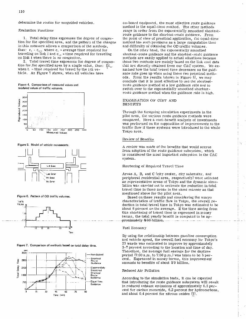
110
determine the routes for nonguided vehicles.
Evaluation Functions
L. Total delay time ex¡lresses the degree of conges-tion for the specified area, and the pattern of the changesin this measure allows a comparison of the methods,thus: c, - cr", where cr =âv€râgêtime requiredfortraveling on link i and c," = time required for travelingon link i when there is no congestion,
2. Total travel time expresses the degree of conges-tion forrthe specified area by a single value, thus: Etr,when tr = time required for travel by the ith ve- I
hicle. As Figure 7 shows, when all vehicles have
Figure 4. Comparison of measured values andmodeled values of traffic volumes.
Figure 5. Model of vehicle movements.
on-board equipment, the most effective route guidancemethod is the equal-time method. The other methodsrange in order from the exponentially smoothed shortest-route guidance to the shortest-route guidance. Fromthe point of view of practical application, the equal-timemethod has such problems as a large computation timeand difficulty of obtaining the OD traffic volumes.
On the other hand, the exponentially smoothedshortest-route guidance and the shortest-route guidancemethods are easily applied to actual situations becausethese two methods are mainly based on the link cost datathat are directly obtained from our CAC system. We ex-amined how the total travel time decreases as the guid-ance rate goes up when using these two practical meth-ods. From the results (shown in Figure 8), we mayconclude that it is most effective to use the shortest-route guidance method at a low guidance rate and toswitch over to the e:<trlonentially smoothed shortest-route guidance method when the guidance rate is high.
EXAMINATION OF COST ANDBENEFITS
Through the foregoing simulation eryeriments in thepilot area, the various route guidance methods werecompared. Here a cost-benefit analysis of investmentswas performed on the supposition of improvements to thetraffic flow if these systems were introduced to the wholeTokyo area.
Review of Benefits
A review was made of the benefits that would accruefrom adoption of the route guidance subsystem, whichis considered the most important subsystem in the CACsystem.
Shortening of Required Travel Time
Areas A, B, and C (city center, city subcenter, andperipheral residential area, respectively) were selectedas representative areas of Tokyo and the dynamic simu-lation was carried out to estimate the reduction in totaltravel time in those areas in the same manner as thatmentioned above for the pilot area.
Based on these results and considering the macrocharacteristics of traffic flow in Tokyo, the overall re-duction in total travel time in Tokyo was estimated to beabout 6 percent on the average. If the time saving fromtNs shortening of travel time is expressed in moneyterms, the total yearly benefit is computed to be ap-
F\rel Economy
By using the relationship between gasoline consumptionand vehicle speed, the overall fuel economy for Tokyots23 wards was estimated to improve by approximately3-7 percent according to the location and time of day.Therefore, the average fuel savings for the daytimeperiod (?:00 a.m. to ?:00 p.m.) was taken to be 5 per-cent. E4lressed in money terms, this improvementamounts to benefits of about *9 billion.
Reduced Air Pollution
According to the simulation tests, it can be expectedthat introducing the route guidance subsystem will resultin reduced exhaust emissions of approximately 6.5 per-cent for carbon monoxide, 6.2 percent for hydrocarbons,and about 0.4 percent for nitrous oxides (?).
3ñ
8ib
É.
o.EF
.EoôõIF-
tlTrafficVdme
l
I
Mæved Vajrg
--] LJ
Figure 6. Pattern of OD traffic volumes.
Time
Figure 7. Comparison of methods based on total delay time.
sec
-Noñ-Gu¡dêd-'-ShortêstRouteGuidance
---- ExponentiallySmoothedShortestRouteGuidance
-. - EquaLT¡meGuidance
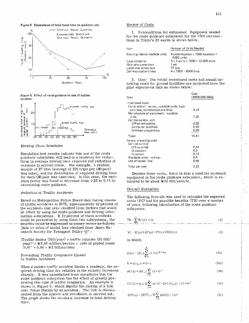
- Shortest Route Gu¡dance
------ Exponentially SmoothedShortest Route Guidance
Guidance Rate
111
oEf-o
f!pt
9E
'õ'ñÈoF
oÊ'u^POE.> b"Èo5 e_bo o_9
o3H$lR.E ì*Þs;
Figure 8. Dependence of total travel time on gu¡dance rate.
Figure 9. Effect of route guidanc€ in case of suddenacc¡dent.
prewt traffic flow
gútr traff¡c
ræoåædSimJatimtire (min.)
Keeping Close Schedules
Simulation test results indicate that use of the routeguidance subsystem \ryill lead to a tendency for reduc-tions in average driving time required and reduction ofvariance in arrival times. For example, a randomsample of 2? ODs (average of 220 trips per OD pair)\{ras taken, and the distribution of required driving timefor each OD pair was e>F.mined. In this case, the vari-ation factor was found to decrease from 0.25 to 0.15 byintroducing route guidance.
Reduction of Traffic Accidents
Based on Metropolitan Police Board data listing causesof traffic accidents in 1976, approximately 40 percent ofthe accidents that year resulted from factors that wouldbe offset by using the route guidance and driving infor-mation subsystems. If 10 percent of these accidentscould be prevented by using these two subsystems, the
Review of Costs
1. Preconditions for estimates: Equipment neededfor the route guidance subsystem for the 1500 intersec-tions in Tokyo's 23 wards is shown below.
Number of Units Needed
Route guidance roadside units
Loop antennaeMain-area computersLocal-area computersCommunications lines
4 units/location x 1 500 locations =6000 units
4 x 2 units x 1500 = 12 000 units1 set32 sets4x 1500=6000lines
2. Cost: The initial investment costs and annual op-erating costs for ground facilities are projected from thepilot experiment data as shown below:
Cost(Y000 000 000s)Item
lnvestment costsConstruction: survey, roadside units, loop
antennae, communications lines 4.74Manufacture of equipment: roadside
un¡tsCentral control unit
Office remodelingComputer purchaseSoftware preparation
TotalAnnual operating costs
Central controlOffice rentalOperati onsPersonnel
Roadside units: upkeepUse of leased lines
Total per year
7.20
o.825.45o.20
18.41
0.44o.20.130.60.86
2.23
closed
Besides these costs, there is also a need for on-boardequipment in the route guidance subsystem, which is es-timated to be about *30 0OO/vehicle.
Overall Evaluation
The following formula was used to calculate the e&eetedcosts (TC) and the possible benefits (TB) over x numberof years following introduction of the route guidancesubsystem.
ldata on value of social loss obtained from Japan Re-search Society for Transport Policy (8)1:
flraffic deaths (¡OO/year) + traffic injuries (SS OOOT
year)] x *2.46 mitlion/person x lrate of guided roads(0,0)l x 0.04 = *2 billion,/year
Preventing Traffic Congestion Causedby Sudden Accidents
When a sudden traffic accident blocks a roadway, the re-quired driving time for vehicles in the vicinity increasessharply. It 'was ascertained from simulation that theroute guidance subsystem has the effect of greatly pre-venting this tl¡pe of traffic congestion. An example isshown in Figure 9, which depicts the closing of a linknear Tokyo Station by an accident. The link is discon-nected from the system and simulation is carried out.The graph shows the resultant increase in total drivingtime.
B(i)/( I + r)i
TC = IC(x) + RC(x) + CC(x) + RCC(x)
in which
!nic
IC(x) = (IC.) X (l *.)-" "'"N=o
N=(i/n¡")i=Q-¡x
RC(x) = (Rc.) >i=0
CC(x) = to,* S)i {a'(i) + [a(i)/n""]] x (l +r)-ii=o
RCC(x) = (RCC.x S)) [a(i)l (l +r)-ii=0
(3ai)
(3aii)
(3b)
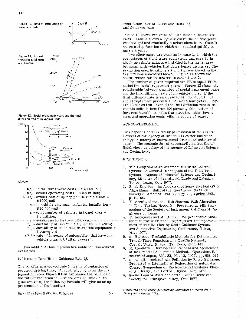
tLz
Figure 10. Rate of ¡nstallation ofin-vehicle units.
lotyea.st
Figure 11. Annualtrends in total costsand benef¡ts.
I 5 yærs
Figure 12. Social repayment years and the f¡naldiffusion rate of in-vehicle units.
50 too
where
IC" = initial investment costs = *20 billion;RC" = annual operating costs = *2.5 billion;
RCC" = annual cost of upkeep per in-vehicle unit =* 1000/unit;
a = in-vehicle unit cost, including installation =*30 000/unit;
s = total number of vehicles in target ârêâ =1.8 million;
Installation Rate of In-Vehicle Units (a)and Guidance Rate
Figure 10 shows two rates of installation of in-vehicleunits. Case A shoïr¡s a logistic curve that in five yearsreaches a/2 and eventually reaches close to c. Case Bshows a step function in which a is reached quickly inthe first year.
T\vo other cases are ercamined: case 1, in which thepêrcentages of p and e are equivalent, and case 2, inwhich in-vehicle units are installed in the target areabeginning with vehicles that drive longer distances. Theevaluation used Equations 2 and 3 and was based on theassumptions mentioned above, Figure 11 shows theannual trends for TC and TB in cases 1 and 2.
The number of years required for TB to equal TC iscalted the social repayment years. Figure 12 shows therelationship between x number of social repayment yearsand the final diffusion rate of in-vehicle units. If thefinal diffusion rate is supposed to be 100 percent, thesocial repayment period will be two to four years. Fig-ure 12 shows that, even if the final diffusion rate of in-vehicle units is less than 100 percent, this system of-fers considerable benefits that meet the initial invest-ment and operating costs within a couple of years.
ACKNOWLEDGMENT
This paper is contributed by permission of the DirectorGeneral of the Agency of Industrial Science and Tech-nology, Ministry of International Trade and Industry ofJapan. The contents do not necessarily reflect the of-ficial views or policy of the Agency of Industrial Scienceand Technology.
REFERENCES
The Comprehensive Automobile Traffic ControlSystem: A General Description of the Pilot TestSystem. Agency of Industrial Science and Technol-ogy, Ministry of International Trade and Industry,Tokyo, Japan, Oct. 1977.S. E. Dreyfus. An Appraisal of Some Shoriest-PathAlgorithms. 8u11. of the Operations ResearchSociety of America, Vol. 1, Suppl. 1, Spring 1968,p. B-166.
a
olz
1.
2.
n." = durability of in-vehicle equipment = 6 years;ni" = durability of other than in-vehicle equipment =
7 years; andd(i) = rate of increase of automobiles that have in-
vehicle units la(i) after i yearsT.
Two additional assumptions are made for this overallevaluation.
Reliance of Benefits on Guidance nate (6)
The benefits are viewed only in terms of reduction ofrequired driving time. Accordingly, by using the in-formation from Figure I that erçresses the reliance ofthe rate of reduction in required driving time on theguidance rate, the followÍng formula will give us an ap-proximation of the benefits:
B(É) = 80x (2-0)x É(Y000 000 000s/year) (4)
3. Y. Anzai and others. Kth Shortest Path Algorithmin Time-Variant Network. Presented at 14th Sym-posium of the Society of Instrument and Control En-gineers in Japan.
4, F. Kobayashi and M. Izumi. Comprehensive Auto-
Flow by Route Guidance System.Engineering Conference, Tokyo,
5. S. Stidham. Probabilistic Methods for DeterminingTravel-Time Functions in a Traffic Network.Cornell Univ,, Ithaca, NY, Tech. Rept. 141.
6. K. Okudaira. Development Process and Applicationof Incremental Assignment Method. Operations Re-search of Japan, YoL.22, No. 12, 197?, pp. 688-694.
7. S. Kokaji. Reduced Air Pollution by Route Guidance.Presented at International Federation of AutomaticControl S5rmposium on Environmental Systems Plan-ning, Design, and Control, Kyoto, Aug. 1977.
8. Social Loss of Road Accidents. Japan ResearchSociety for Transport Policy, Oct. 1977.
Publication of this paper sponsored by Committee on Traffic FlowTheo ry a n d C hara cter i st i cs.
ment of Traffic3rd AutomotiveNov. 1977.
113
Outline of the Comprehensive AutomobileTraffic Control Pilot Test SystemNöbuo Yumoto, Sumitomo Electric Industries, Ltd., Osaka, JapanHirokazu lhara, Systems Development Laboratory, Hitachi, Ltd,,
Kawasaki, JapanTsutomu Tabe, Nippondenso Company, Ltd., Aichi, JapanMasaru Naniwada, Central Research Laboratories, Nippon Electric
Company, Ltd,, I(awasaki, Japan
ln the final phase of the Comprehens¡ve Automobile Traffic Control Proj-ect, a pilot system was constructed and put into operation in october1977. ln the p¡lot area, which covers 28 km2 in southwestern Tokyo, atwo-way exchange of dig¡tal information occurs between instrumentedvehicles and roadside equipment. The driver receives a visual display ofrouting information that is based on current traffic conditions and otherinformation for safe driving. ln order to provide the drivers of non¡nstru-mented veh¡cles w¡th the routing informat¡on, new roadside displays weredeveloped. A roadside radio system, which gives the driver traffíc in-formation and provides instructions in an emergency, was also developed.This paper presents an overview of the p¡lot system and describes theprocedure of optimum route finding, the specificat¡on of the digital com-municat¡on link between road and vehicle, and the hardware features ofthe principal equipment. A preliminary evaluation of the system per-formance is also described.
The Comprehensive Automobile Traffic Control (CAC)Project 0,2), sponsored by the Agency of IndustrialScience and Technology of the Ministry of InternationalTrade and Industry, was begun in 1973 for a six-yearresearch perÍod with a budget of seven billion yenly zzo = g1.oo (August 19?9)1.
The objective of this project is to develop an inte-grated system that provides, by means of an improvedcommunication medium between vehicles and the ex-ternal world, such functions as optimum route guidanee,diversion of traffic out of high-density pollution areas,priority for public service vehicles, advanced displayof traffic regulations and alerts, and the potential forsimultaneous communication in case of emergency.Such a system will contribute to an improved public ac-ceptance of automobile transportation by reducing traf-fic congestion, traffic accidents, and air pollution.
The principal technical activities undertaken toachieve this objective were to develop (a) an optimumcontrol strategy of traffic flow, as well as monitoringof vehicular movement and assignment of optimumroute; (b) a high-speed and reliable two-way communi-
between the driver and the ground:
1. Two-way digital communication link by inductiveradio (when the vehicle's antenna passes over the roadantenna, a data transmission of about 100 bits in eachdirection occurs via the magnetic field between bothantennas ),
2, Ground-to-vehicle oral communication by meansof a roadside radio (radio transmission reaches onlythe vehicles that pass the roadside antenna, '¡hich ex-tends along the street), and
3. Roadside visual display.
Functions of the Pilot System
The pilot system has five subfunctions:
1. Route guidance, which gives the driver a visualinstruction at decision points and guides the driver tohis or her destination in the same way that the Experi-mental Route Guidance System (fnCS) Ooes (3) ltheCAC system differs from ERGS in that the route isperiodically optimized on the basis of the cument traf-fic and road conditions and in that the system has func-tions other than route guidanceJ;
2, Driving information, which gives the driver avisual display of information useful for safe driving andgives him or her a sonic alert when the vehicle exceedsthe speed limit according to ground control;
3. Priority for public service vehicles, which givespriorÍty to publie service vehicles at the signalizedintersections and improves the operating efficiency ofsuch vehicles by continuous monitoring of their indi-vidual locations;
4, Urgent information, which gives the driver in-structions in an emergency and provides audio informa-tion on localized traffic and road conditions in usual
ground; and (c) an excellent displav method that con-siders human engineering factors. In 19?4, prototypehardware was developed and evaluated in a preliminarye4perimental installation',vithin the grounds of a factory.
Between 1975 and 19?6, the soft.,vare and hardwarefor the pilot system were manufactured and installed ina 28-km" test area in the southwestern part of Tokyo.The purposes of the pilot test include evaluating the ef-fectiveness of the system in an actual urban situation,identifying potential problems regarding future adoptionof the system, demonstrating the system to the public,and obtaining their opinions about it. The pilot systemhas been in actual operation since October 197?.
OUTLINE OF THE PILOT SYSTEM
Communication Between the Driver
The pilot system has three means of communication
5, Roadside route display, ',vhich gives drivers ofnoninstrumented vehicles the routing information,
The route guidance, driving information, and priorityfor public service vehicles subsystems use the digitalcommunication link by inductive radio. The vehicletype, its identification number, and destination codeare sent from the vehicle to the ground. Routing anddriving information are sent in the opposite direetion.At some locations where only driving information isnecessary, downward data are neglected by the ground.
The urgent information subsystem uses the roadsideradio, The audio medium of communication supple-ments the visual display of route guidance and drivinginformation and provides the driver with more versatileinformation than digital communication does.
Configuration of the Pilot Systern
Arterial streets and ex¡rressways of about 100 km in
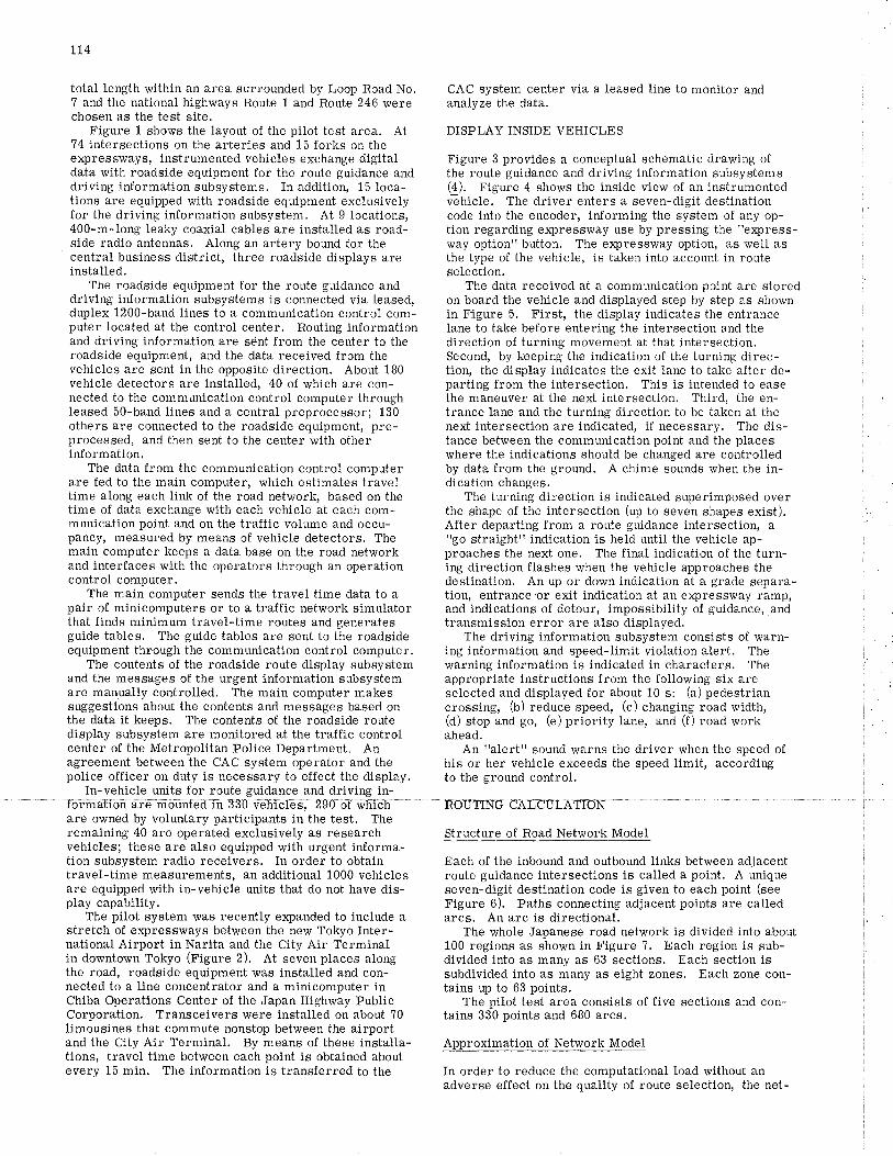
tt4
total length within an area surrounded by Loop Road No, CAC system center via a leased line to monitor and? and the national highways Route 1 and Route 246 were arLalyze the data.chosen as the test site.
data with roadside equipment for the route guidance and the route guidance and driving information subsystems
Figure 1 shows the layout of the pilot test area. At74 intersections on the arteries and 15 forks on theexpress'rvays, instrumented vehicle s exchange digital
driving information subsvstems. In addition, 15 loca-tions are equipped with roadside equipment exclusivelyfor the driving information subsystem. At g locations,400-m-long leaky coaxial cables are installed as road-side radio antennas. Along an artery bound for thecentral business district, three roadside displays areinstalled.
The roadside equipment for the route guidance and
and driving information are sént from the center to theroadside equipment, and the data received from thevehicles are sent in the opposite direction. About 180vehicle detectors are installed, 40 of which are con-nected to the communication control computer throughleased 50-band lines and a central preprocessor; 130others are connected to the roadside equipment, pre-processed, and then sent to the center with otherinformation,
The data from the communication control computerare fed to the main computer, rvhich estimates traveltime along each link of the road network, based on thetime of data exchange with each vehicle at each com-munication point and on the traffic volume and occu-pancy, measured by means of vehicle detectors. Themain computer keeps a datâ base on the road networkand interfaces with the operators through an operationcontrol computer.
The main computer sends the travel time data to a
that finds minimum travel-time routes and generatesguide tables. The guide tables are sent to the roadside
and the messages of the urgent information subsystemare manually controlled, The main computer makessuggestions about the contents and messages based onthe data it keeps. The contents of the roadside routedisplay subsystem are monitored at the traffic controlcenter of the Metropolitan Police Department. Anagreement between the CAC system operator and the
remaining 4O are operated exclusively as researchvehicles; these are also equipped with urgent informa-tion subsvstem radio receivers, In order to obtaintravel-time measurements, an additional 1000 vehiclesare equipped with in-vehicle units that do not have dis-play capability.
The pilot system was recently expanded to include astretch of ex¡lressways between the new Tokyo Inter-national Airport in Narita and the City Air Terminalin downtown Tokyo (Figure 2). At seven places alongthe road, roadside equipment was installed and con-nected to a line concentrator and a minicomputer inChiba Operations Center of the Japan Highway PublicCorporation. Transceivers were installed on about ?0limousines that commute nonstop between the airportand the City Air Terminal. By means of these installa-tions, travel time between each point is obtained aboutevery 15 min. The information is transferred to the
DISPLAY INSIDE VEHICLES
Figure 3 provides a conceptual schematic drawing of
g). Figure 4 shows the inside view of an instrumentedvehicle. The driver enters a seven-digit destinationcode into the encoder, informing the system of any op-tion regarding expressway use by pressing the "ex¡rress-way option" button. The express'"vay option, as well asthe type of the vehicle, is taken into account in routeselection,
The data received at a communication point are stored
direction of turning movement at that intersection.Second, by keeping the indication of the turning direc-tion, the display indicates the exit lane to take after de-parting from the intersection. This is intended to easethe maneuver at the next intersection. Third, the en-trance lane and the turning direction to be taken at thenext intersection are indicated, if necessary, The dis-tance between the communication point and the placeswhere the indications should be changed are controlledby data frorn the ground, A chime sounds when the in-dication changes.
The turning direction is indicated superimposed overthe shape of the intersection (up to seven shapes exist).After departing from a route guidance intersection, a"go straight" indication is held until the vehicle ap-proaches the next one. The final indication of the turn-ing direction flashes when the vehicle approaches thedestination. An up or down indication at a grade separa-tion, entrance'or exit indication at an ex¡rressway ramp,
transmission error are also displayed.The driving information subsvstem consists of warn-
appropriate instructions from the following six areselected and displayed for about 10 s: (a) pedestriancrossing, (b) reduce speed, (c) changing road width,(d) stop and go, (e) priority lane, and (f) road workahead.
An "alert" sound warns the driver when the speed ofhis or her vehicle exceeds the speed limit, according
Structure of Road Network Model
Each of the inbound and outbound links between adjacentroute guidance intersections is called a point. A uniqueseven-digit destination code is given to each point (seeFigure 6). Paths connecting adjacent points are calledarcs, An arc is directional.
The '"vhole Japanese road network is divided into about100 regions as shown in Figure 7, Each region is sub-divided into as many as 63 sections, Each section issubdivided into as many as eight zones. Each zone con-tains up to 63 points.
The pilot test area consists of five sections and con-tains 330 points and 680 arcs.
Approximation of Network Model
In order to reduce the computational load without anadverse effect on the quality of route selection, the net-
driving information subsystems is connected via leased, on board the vehicle and displayed step by step as shownduplex 1200-band lines to a communication control com- in Figure 5. First, the display indicates the entranceputer located at the control center. Routing information lane to take before entering the intersection and the
pair of minicomputers or to a traffic network simulator and indications of detour, impossibility of guidance, and
equipment through the communication control computer. ing information and speed-limit violation alert. TheThe contents of the roadside route display subsystem warning information is indicated in characters. The
police officer on duty is necessary to effect the display, to the ground control.In-vehicle units fôr route guidánce and driving in- "
I
Iormatron âre mounted ln öJU vehicles, zgu ot whichare owned by voluntary participants in the test, The
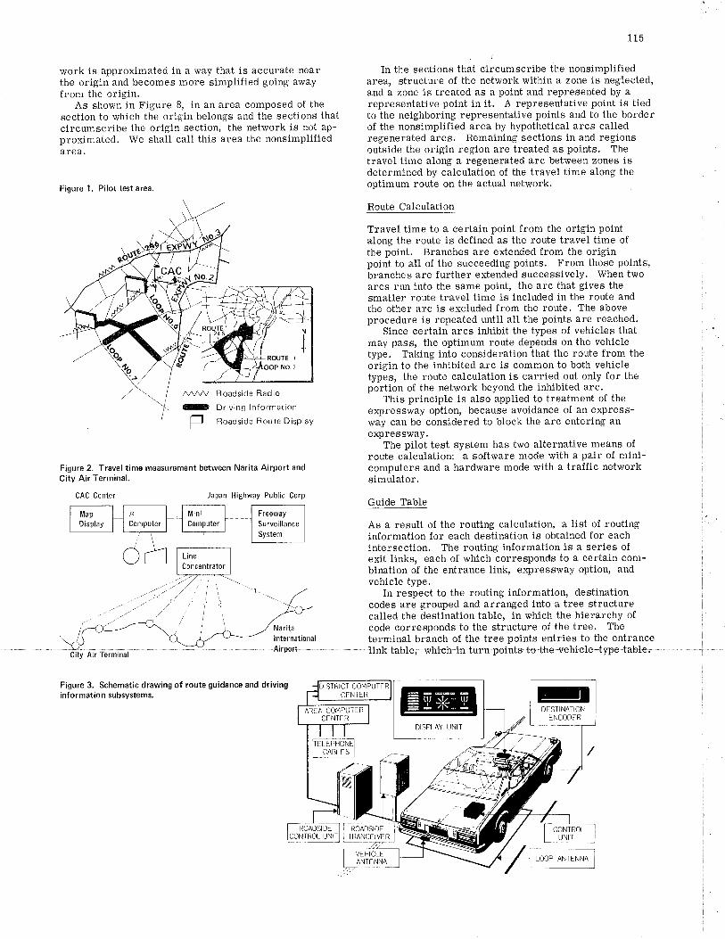
work is approximated in a way that is accurate nearthe origin and becomes more simplified going awayfrom the origin.
As shown in Figure 8, in an area composed of thesection to which the origin belongs and the sections thatcircumscribe the origin section, the network is not ap-proximated. We shall call this area the nonsimplifiedârea.
115
In the sections that circumscribe the nonsimplifiedarea, structure of the network within a zone is neglected,and a zone is treated as a point and represented by arepresentative point in it. A representative point is tiedto the neÍghboring representative points and to the borderof the nonsimplified area by hypothetical arcs calledregenerated arcs, Remaining sections in and regionsoutside the origin region are treated as points. Thetravel time along a regenerated arc between zones isdetermined by calculation of the travel time along theoptimum route on the actual network.
Route Calculation
Figure 1. Pilot test area.
Roadside Radio
Driving lnformation
Roadside Route Display
Figure 2. Travel time measurement between Nar¡ta Airport andCity Air Terminal.
CAC Center Japan Highway Public Corp
Travel time to a certain point from the origin pointalong the route is defined as the route travel time ofthe point. Branches are extended from the originpoint to all of the succeeding points. From those points,branches are further extended successively' When twoarcs run into the same point, the arc that gives thesmaller route travel time is included in the route andthe other arc is excluded from the route. The aboveprocedure is repeated until all the points are reached'
Since certain arcs inhibit the types of vehicles thatmay pass, the optimum route depends on the vehicletype. Taking into consideration that the rdute from theorigin to the inhibited arc is common to both vehicletypes, the route calculation is carried out only for theportion of the network beyond the inhibited arc.
This principle is also applied to treatment of theer<press'rvay option, because avoidance of an express-way can be considered to bloek the arc entering anexpressvfay.
The pilot test system has two alternative means ofroute calculation: a software mode with a pair of mini-computers and a hardware mode with a traffic networksimulator,
Guide Table
As a result of the routing calculation, a list of routinginformation for each destination is obtained for eachintersection, The routing information is a series ofexit links, each of which corresponds to a certain com-bination of the entrance link, expressway option, andvehicle type.
In respect to the routing information, destinationcodes are grouped and arranged into a tree structurecalled the destination table, in which the hierarchy ofcode corresponds to the structure of the tree. Theterminal branch of the tree points entries to the entrance
City Air Terminal
Figure 3. Schematic drawing of route guidance and drivinginformation subsystems. ã U.l rlz - (t,
: .å /l\ '-
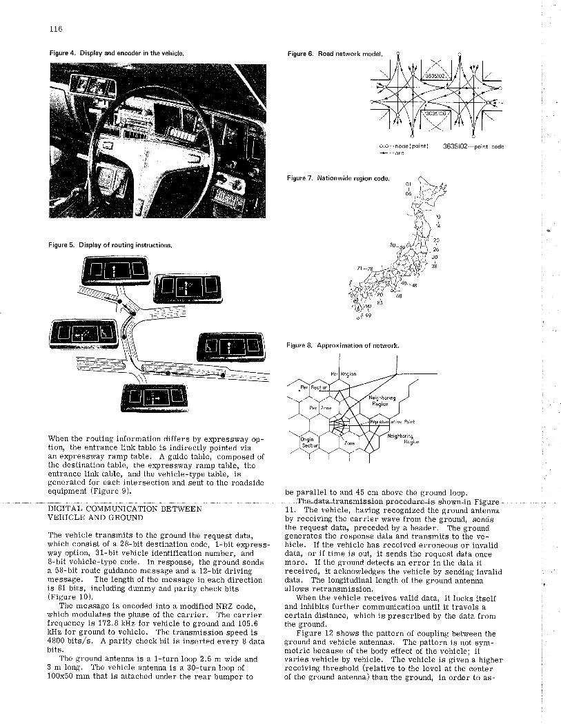
Figure 4. Display and encoder in the veh¡cle.
!t
=/
,aI
116
Figure 6. Road network model.
Figure 7.
o,o'..node(po¡nt) 3635102.'.point code+ ,..arc
Figure 5. Display of routing instruct¡ons.
When the routing information differs by expressway op-tion, the entrance link table is indirectly pointed viaan expressway ramp table, A guide table, composed ofthe destination table, the erçressway ramp table, theentrance link table, and the vehicle-type table, isgenerated for each intersection and sent to the roadsideequipment (Figure 9). be parallel to and 45 cm above the ground loop.
IThe data transmission4*oeedure is she,v*n-i#
90I
99
irFaúFigure 8. Approximation of network.
DIGITAL COMMUNICATION BE TWEENVEHICLE AND GROUND
The vehicle transmits to the ground the request data,which consist of a 28-bit destination code, 1-bit express-rÃray option, 31-bit vehicle identification number, and8-bit vehicle-type code, In response, the ground sendsa 58-bit route guidance message and a 12-bit drivingmessage. The length of the message in each directionis 81 bits, including dummy and parity check bits(Figure 10).
The message is encoded into a modified NRZ code,which modulates the phase of the carrier. The camierfrequency is 172.8 kHz for vehicle to ground and 105.6kHz for ground to vehicle. The transmission speed is4800 bits/s. A parity check bit is inserted eveiy I databits.
The ground antenna is a l-turn loop 2.5 m wide and3 m long. The vehicle antenna is a 3O-turn loop of100x50 mm that is attached under the rear bumper to
11, The vehicle, having recognized the ground antennaby receiving the carrier wave from the ground, sendsthe request data, preceded by a header. The groundgenerates the response data and transmits to the ve-hicle. If the vehicle has received erroneous or invaliddata, or if time is out, it sends the request data oncemore. If the ground detects an error in the data itreceived, it acknowledges the vehicle by sending invaliddata. The longitudinal length of the ground antennaallows retransmission.
When the vehicle receives valid data, it locks itselfand inhibits further communication until it travels acertain distance, which is prescribed by the data fromthe ground.
Figure 12 shows the pattern of coupling between theground and vehicle antennas. The pattern is not sym-metric because of the body effect of the vehicle; itvaries vehicle by vehicle. The vehicle is given a higherreceiving threshold (relative to the level at the centerof the ground antenna) than the ground, in order to as-
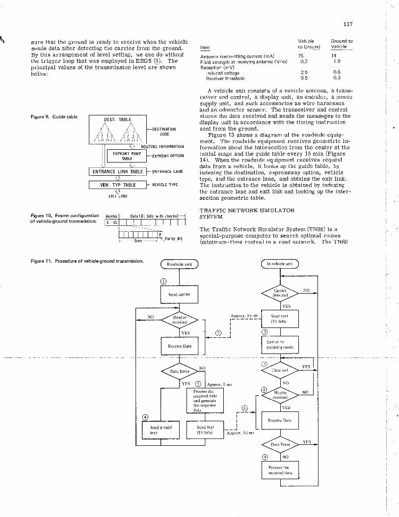
\ sure that the ground is ready to receive when the vehiclesends data after detecting the carrier from the ground.By this arrangement of level setting, we can do withoutthe trigger loop that was employed in ERGS (3). Theprincipal values of the transmission level are shownbelow:
Figure 9. Guidetable.
Antenna transmittihg current (mA) 75 14
Field strength at receiving antenna (V/m) O.2 1.9
Reception (mV)lnduced voltageReceiver threshold
2.5 0.60.5 0.3
A vehicle unit consists of a vehicle antenna, a trans-ceiver and control, a display unit, an encoder, a powersupply unit, and such accessories as wire harnessesand an odometer senser, The transceiver and controlstores the data received and sends the messages to thedisplay unit in accordance with the timing instructionsent from the ground.
Figure 13 shows a diagram of the roadside equip-ment. The roadside equipment receives geometric in-formation about the intersection from the center at theinitial stage and the guide table every 15 min (Figure14). When the roâdside equipment receives requestdata from a vehicle, it looks up the guide table, byindexing the destination, express\ilay option, vehicletype, and the entrance lane, and obtains the exit link.The instruction to the vehicle is obtained by indexingthe entrance lane and exit link and looking up the inter-section geometric table.
TRAFFIC NE TWORK SIMULATORSYSTEM
The Traffic Net'rvork Simulator System (TUSS) is aspecial-purpose computer to search optimal routes(minimum-time routes) in a road network. The TNSS
ItemVehicleto Ground
tL7
Ground toVehicle
TINATIONCODE
INFORMATION
XPRSWY OPTION
NTRANCT LANE
EHICLE TYPE
Figure 10. Frame configurationof vehicle-ground transm¡ssion.
DEST. TABLE
ING
EXP
.IN'I
'VEH
17 xr
I exenswv naueI TAELEL__________r_
ENTRANCT LINK TABLE
VEH. TYP TABLE
EXIT LINK
Figure 1 1. Procedure of vehicleground transmission.
o
Approx. l6 msf------I
I(ùr----J
(qF--III
--JApprox. 16 ms
Send text(81 bits)
Send text(81 bits)
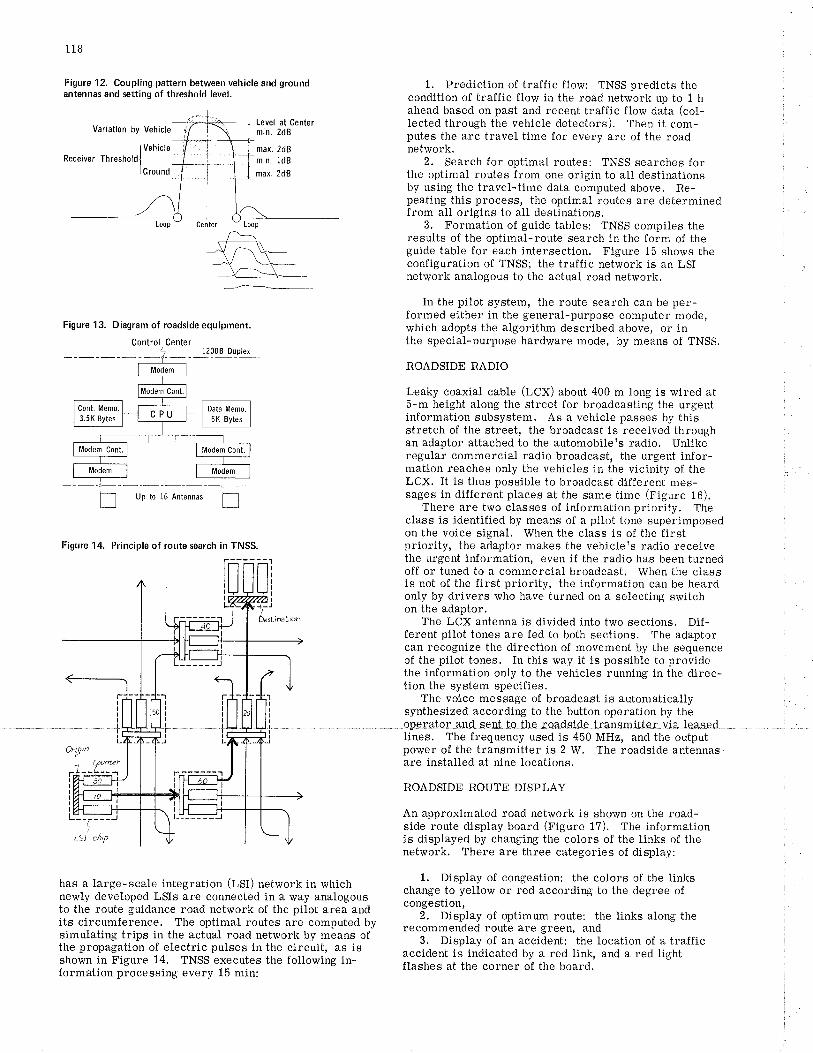
Variat¡on by Vehicle
f VehicleReceiver Thresholdl
I crnun.l
118
Figure 12. Coupling pattern between vehicle and groundantennas and settíng of threshold level.
Ät/=\L_-v \\_\- \- __j¿
-\_
Level at Centermin. 2dB
max. 2dB
min. ldBmax. 2dB
1. Prediction of traffic flow: TNSS predicts thecondition of traffie flow in the road network up to t hahead based on past and recent traffic flow data (col-lected through the vehicle detectors). Then it com-putes the arc trâvel time for every arc of the roadnetwork.
2, Search for optimal routes: TNSS searches forthe optimal routes from one origin to all destinationsby using the travel-time data computed above. Re-peating this process, the optimal routes are determinedfrorn all origins to all destinations,
3. Formation of guide tables: TNSS compiles theresults of the optimal-route search in the form of theguide table for each intersection. Figure 15 shows theconfiguration of TNSS; the traffic net',vork is an LSInetwork analogous to the actual road network,
In the pilot system, the route search can be per-formed either in the general-purpose computer mode,which adopts the algorithm described above, or inthe special-purpose hardware mode, by means of TNSS.
ROADSIDE RADIO
Leaky coaxial cable (LCX) about 400 m long is wired at5-m height along the street for broadcasting the urgentinformation subsystem, As a vehicle passes by thisstretch of the street, the broadcast is received throughan adaptor attached to the automobile's radio, Unlikeregular commercial radio broadcast, the urgent infor-mation reaches only the vehicles in the vicinity of theLCX. It is thus possible to broadcast different mes-sages in different places at the same time (Figure 16).
There are two classes of information priority. Theclass is identified by means of a pilot tone superimposedon the voice signal. When the class is of the firstpriority, the adaptor makes the vehicle's radio receivethe urgent information, even if the radio has been turnedoff or tuned to a commercial broadcast. When the classis not of the first priority, the information can be heardonly by drivers who have turned on a selecting switchon the adaptor.
The LCX antenna is divided into two sections, Dif-ferent pilot tones are fed to both sections. The adaptorcan recognize the direction of movement by the sequenceof the pilot tones. In this way it is possible to providethe information only to the vehicles running in the direc-tion the system specifies.
The voice message of broadcast is automaticallysynthesized according to the button operation by the
Cont. Memo.
3.5K Bytes
Figure 14. Principle of route search in TNSS.
::-l
has a large-scale integration (LSI) network in whichnewly developed LSIs are connected in a way analogousto the route guidance road network of the pilot area andits circumference. The optimal routes are computed bysimulating trips in the actual road network by means ofthe propagation of electric pulses in the circuit, as isshown in Figure 14. TNSS executes the following in-formation processing every 15 min:
lines. The frequency used is 450 MHz, and the outputpower of the transmitter is 2 W. The roadside antennasare installed at nine locations.
ROADSIDE ROUTE DISPLAY
An approximated road network is shown on the road-side route display board (Figure 1?). The informationis displayed by changing the colors of the links of thenetwork. There are three categories of display:
1. Display of congestion: the colors of the linkschange to yellow or red according to the degree ofcongestion,
2. Display of optimum route: the links along therecommended route are green, and
3. Display of an accident: the location of a trafficaccident is indicated by a red link, and a red lightflashes at the corner of the board.
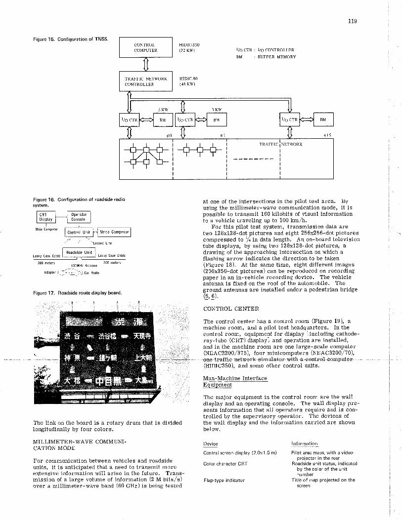
119
Figure 15. Configuration of TNSS.
Figure 16. Configuration of roadside radiosystem.
I/6 CTR : l/O CONTROLLER
BM : BIJFFER MEMORY
TRAFFTC iNETWORK
200 meters 200 meters.400MHz Antenna
Adaptor ¡;l-. \'çr, ¡r¿¡o
Figure 17. Roadside route display board.
The link on the board is a rotarv drum that is dividedlongitudinally by four colors.
MILLIME TE R- IA/AVE COMM UNI-CATION MODE
For communication between vehicles and roadsideunits, it is anticipated that a need to transmit moreextensive information will arise in the future. Trans-mission of a large volume of information (2 M bits/s)over a millimeter-wave band (60 GHz) is being tested
at one of the intersections in the pilot test area. Byusing the millimeter-wave communication mode, it ispossible to transmit 160 kilobits of visual informationlo a vehicle traveling up to 100 km/h.
For this pilot test system, transmission data aretwo 128x128-dot pictures and eight 256x256-dot picturescompressed to lfqin data length. An on-board televisiontube displays, by using two 128x128-dot pictures, adrawing of the approaching intersection on which aflashing arrow indicates the direction to be taken(Figure 18). At the same time, eight different images(256x256-dot pictures) can be reproduced on recordingpaper in an in-vehicle recording device. The vehicleantenna is fixed on the roof of the automobile. Theground antennas are installed under a pedestrian bridge(!,!).
CONTROL CENTER
The control center has a control room (figure 19), amachine room, and a pilot test headquarters. In thecontrol room, equipmènt for display lincluding cathode-ray-tube (Cnt) aisptayl and operation are installed,and in the machine room are one large-scale computer(NEAc220o/3?5), four mÍnicomputers (Nracgzoo/zo),
(HIDIca5o), and some other control units.
Man-Machine InterfaceffiThe major equipment in the control room are the walldisplay and an operating console. The wall display pre-sents information that all operators require and is con-trolled by the supervisory operator. The devices ofthe wall display and the information carried are shownbelow.
lnformation
/
Central screen display (2.0x1.5 m)
Color character CRT
Flap-type indicator
Pilot area maps, with a video-projecter in the rear
Roadside unit status, indicatedby the color of the unitnumber
Title of map projected on thesc reen
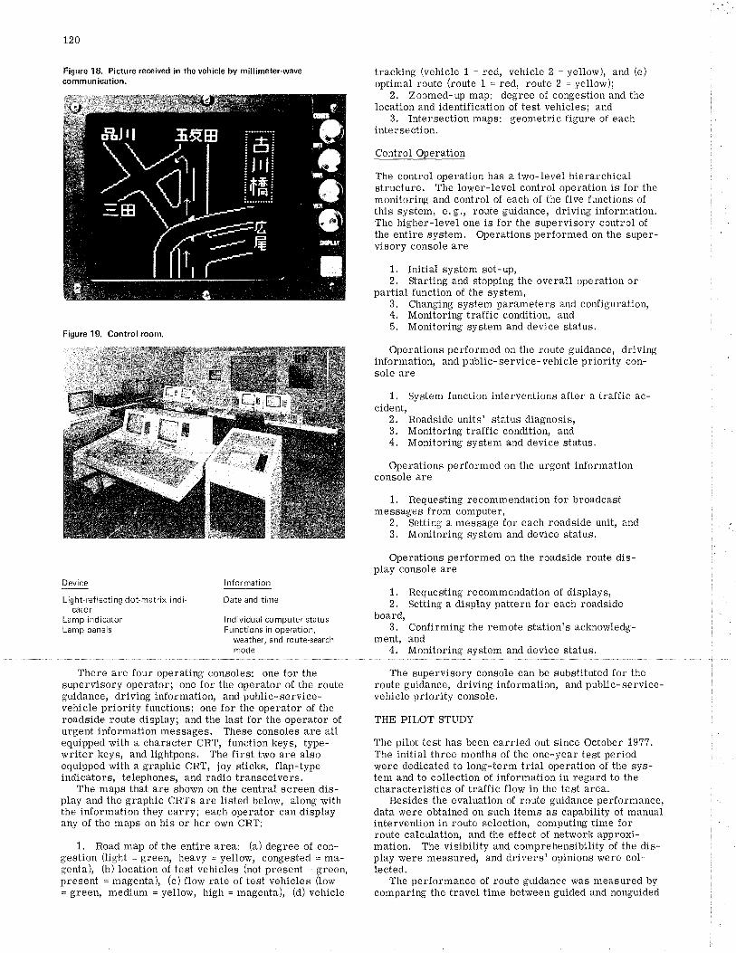
L20
Figure 18. Picture received in the veh¡cle by mill¡meter-wavecommun¡cation.
Figure 19, Control room.
tracking (vehicle 1 = red, vehicle 2 = yellow), and (e)optimal route (route 1 = redr route 2 = yellow);
2, Zoomed-up map: degree of congestion and thelocation and identification of test vehicles; and
3. Intersection maps: geometric figure of eachintersection.
Control Opelation
The control operation has a two-level hierarchicalstructure. The lower-level control operation is for themonitoring and control of each of the five functions ofthis system, e. g., route guidance, driving information.The higher-level one is for the supervisory control ofthe entire system. Operations performed on the super-visory console are
1. Initial system set-up,2, Starting and stopping the overall operation or
partial function of the system,3. Changing system parameters and configuration,4, Monitoring traffic condition, and5, Monitoring system and device status,
Operations performed on the route guidance, drivinginformation, and public-service-vehicle priority con-sole are
1, System function interventions after a traffic ac-cident,
2. Roadside unitsr status diagnosis,3. Monitoring traffic condition, and4, Monitoring system and device status,
Operations performed on the urgent informationconsole are
1. Requesting recommendation for broadcastmessages from computer,
2, Setting a message for each roadside unit, and3, Monitoring system and device status.
Operations performed on the roadside route dis-play console are
1.2.
board,3.
ment,4.
Requesting recommendation of displays,Setting a display pattern for each roadside
Confirming the remote station's acknowledg-andMonitoring system and device status.
I
Device
Light-ref lecting dot-matrix indi-cator
Lamp indicatorLamp panels
lnformation
Date and time
I nd ividual computer statusFunctions in operation,
weather, and route-searchmode
There are four operating consoles: one for thesupervisory operator; one for the operator of the routeguidance, driving information, and public-service-vehicle priority functions; one for the operator of theroadside route display; and the last for the operator ofurgent information messages. These consoles are allequipped with a character CRT, function keys, type-writer keys, and lightpens. The first two are alsoequipped with a graphic CRT, joy sticks, flap-typeindicators, telephones, and radio transceivers.
The maps that are shown on the central screen dis-play and the graphic CRTs are listed below, along withthe information they carty; each operator can displayany of the maps on his or her own CRT:
1. Road map of the entire area: (a) degree of con-gestion (tight = green, heavy = yellow, congested = ma-genta), (b) location of test vehicles (not present = green,present = magenta), (c) flow rate of test vehicles (low= green, medium = yellow, high = magenta), (d) vehicle
The supervisory console can be substituted for theroute guidance, driving information, and public-service-vehicle priority console,
THE PILOT STUDY
The pilot test has been carried out since October 19??.The initial three months of the one-year test periodwere dedicated to long-term trial operation of the sys-tem and to collection of information in regard to thecharacteristics of traffic flow in the test area,
Besides the evaluation of route guidance performance,data were obtained on such items as capability of manualintervention in route selection, computing time forroute calculation, and the effect of network approxi-mation. The visibility and comprehensibility of the dis-play were measured, and drivers' opinions were col-lected.
The performance of route guidance was measured bycomparing the travel time bet."veen guided and nonguided
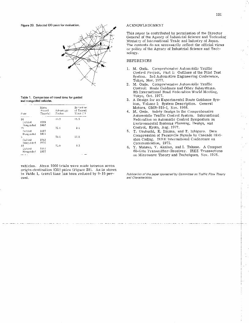
Figure 20. Selected OD pairs for evaluation.
Table 1. Comparison of travel time for gu¡dedand nonguided veh¡cles.
? 5.0
vehicles. About 1000 trials were made between sevenorigin-destination (OD) pairs (Figure 20). As is shownin Table 1, travel time has been reduced by 9-15 per-cent.
lzt
ACKNOWLEDGMENT
This paper is contributed by permission of the DirectorGeneral of the Agency of Industrial ScÍence and TechnologMinistry of International Trade and Industry of Japan.The contents do not necessarily reflect the official viewsor polÍcy of the Agency of Industrial Science and Tech-nology.
REFERENCES
1. M, Onda, Comprehensive Automobile TrafficControl Project, Part 1: Outlines of the Pilot TestSystem. 3rd Automotive Engineering Conference,Tokyo, Nov. 19??.
2. M. Onda. Comprehensive Automobile TrafficControl: Route Guidance and Other Subsystems.8th International Road FederatÍon World Meeting,Tokyo, Oct. 197?.
3. A Design for an Experimental Route Guidance Sys-tem, Volume I: System Description. GeneralMotors, GMR-815-I, Nov. 1968.M. Onda. Safety Design in the ComprehensiveAutomobile Traffic Control System. InternationalFederation on Automatic Control Symposium onEnvironmental Systems Planning, Design, andControl, Kyoto, Aug. 197?.T. Usubuchi, K. Iinuma, and T. Ishiguro, DataCompression of Facsimile Signals by Cascade Divi-sion Coding. IEEE International Conference onCommunication, 19?5.Y. Matsuo, Y. Akaiwa, and I. Takase. A Compact60-GHz Transmitter-Receiver. IEEE Transactionson Microwave Theory and Techniques, Nov. 19?6,
Publication of this paper sponsored by Committee on Traff ic Flow Theoryand Characteristics,
Pair
MeanTrâvelTime(s)
ReductionAdvantage of TrâvelFactor tirne (4) 4.
24GuidedNonguided
29GuidedNonguided
5
GuidedNonguided
18GuidedNonguided
12 39r46',t
'12.1132'.1
7464
t 5.5? 6.3
9.4
76.1
5.
6.
10. B
9.3
17631976
165?