Transfers and Development – Easy Come, Easy Go?

Luc Christiaensen United Nations University – World Institute for Development Economics Research

Katajanokanlaituri 6 B, FI-00160 Helsinki, Finland tel.: +358 96599213

email: luc@wider.unu.edu

and

Lei Pan Corresponding author

Development Economics Group, Wageningen University Hollandseweg 1, 6706KN Wageningen, The Netherlands

tel.: +31 317484354 email: lei.pan@wur.nl

Acknowledgement The authors would like to thank the participants of the Annual Meeting of the American Economic Association 2010 for useful comments, and the Chinese authorities of the World Bank’s Western Poverty Reduction Project in China (WPRP), Wang Pingping, Assistant Counsel, Department of Rural Surveys of the National Bureau of Statistics of China, and Sari Söderstrom, World Bank Task Manager of the WPRP for making the data available.

1

Transfers and Development – Easy Come, Easy Go?

April 15, 2010

Abstract

A central behavioral assumption of economic theory is that income is fungible. Yet, Thaler (1999) highlights that people code income in different mental accounts, creating a direct link between spending behaviour and income sources. This paper examines the differences in the marginal propensity to consume from earned and unearned income, a distinction that has not received much attention, using a panel dataset from rural China. The results indicate that households have a higher marginal propensity to consume unearned income and a higher marginal propensity to invest earned income. There is also larger propensity to spend (transitory) unearned income on non-basic consumption goods and (permanent) earned income on basic consumption goods. Together these results lend credence to the age-old saying ‘Easy come, easy go’. Heeding this advice might be time well spent in future theoretical and empirical research.

1 Spending and the Origins of Income

Folk wisdom holds that income that is easily earned, is also easily spent, a notion that is as

powerful as it is simple, and one that resonates throughout the world’s cultures and languages —

‘Easy come, easy go’ (English), ‘Как нажито, так и прожито’ (Russian), ‘Lai de rong yi, qu de

kuai’ (Chinese). Yet, a central behavioral assumption of economic theory is that income is

fungible.1 In this view, consumption behavior does not depend on how income has been

obtained, but only on the total amount. In technical terms, the marginal propensity to consume

(MPC) is independent of the source of income. Can the economic profession discard century old

folk wisdom as an anomaly? Or does it fundamentally alter economic models and policy

recommendations?

Following the pioneering work by Thaler (1985, 1990) the fungibility assumption is

increasingly challenged by behavioral economists. Building on insights from cognitive

psychology, they argue that people compartmentalize spending into different budget categories

(e.g. food, housing, luxuries, investments) and total income into different mental accounts such

as a current income, a future income and an asset account. Further important categorizations of

current income concern whether income gains are large or small, transient or permanent and

1 Fungibility is the notion that money has no labels and that all sources of income can be (indistinguishably) collapsed in one number.

2

expected or unexpected. The mere existence of such accounts would be inconsequential if

people would not act upon them, i.e. if they were perfectly fungible (substitutable). The

empirical evidence reviewed by Thaler (1999) suggests however that they are not and thus that

mental accounts matter, beyond being mere anomalies.

One example of the existence of mental accounts, which has been receiving more attention

lately, is the ‘fly-paper” or “labeling effect’, a phenomenon whereby people change their

consumption behavior in line with the suggestion of the label (Abeler and Marklein, 2008).

Kooreman (2000) finds for example that the MPC of child clothing out of exogenous child

benefits in the Netherlands is substantially larger than the MPC of child clothing out of other

income sources.2 Other studies explore how income windfalls affect consumption and saving

behavior (Imbens, Rubin, and Sacerdote, 2001; Agarwal, Liu, and Souleles, 2007; Kuhn et al.,

2008) and how the MPC out of windfalls also depends on the size of the gains, with the MPC

from small unexpected income gains typically much larger than the MPC from large income

gains (Thaler, 1999).

This paper focuses on a form of mental accounting which has received much less attention

so far, despite age-old folk wisdom to the contrary, the coding of income in line with the amount

of effort dispensed.3 A better understanding of whether the amount of dispensed effort affects

spending and investment behavior can have important implications for the design of many policy

interventions. For example, massive programs are being developed in many transforming

countries to stem the growing rural-urban divide. Yet, is it more efficient to do so through

(unconditional or conditional) transfers (e.g. China- Harmonious Socialist Countryside4 program;

Brazil—Bolsa Familia) or through employment guarantee schemes as in India? Similarly, are

stimulus packages in times of economic crises aimed at providing employment (Trabajar,

2 Similarly, recent studies of school feeding (Jacoby, 2002; Afridi, 2005) and supplementary nutrition (Islam and Hoddinott, 2009) programs find

that a substantial part of the supplementary feeding ‘sticks’ with the targeted child (like a fly-paper). Because these transfers are inframarginal,

parents would be expected to reallocate the transfer away from the child.

3 Incipient studies include Zhu et al. (2008) who find for example that the marginal propensity to save out of remittances in rural China is only

half that out of other sources of income based on cross-sectional data. Hoffman (2007) finds that mosquito nets received by a household as a

transfer in Uganda are more likely to be used by vulnerable members of the household, but purchased nets are more likely to be used by income

earners in the household. Households treat purchased and free goods differently.

4 An important component of China’s 11th five year plan (2005-2010) is the construction of an harmonious socialist countryside, more recently

also through a dramatic increase in land based subsidies to farmers since 2005. As a result, agricultural subsidies are now more than twice those

in the United States in per acre terms, even though the transfers are only a couple of percent in relation to average rural incomes but 10 to 15

percent of the income of the rural poor.

3

Argentina) more effective in stimulating demand than packages aimed at transferring money to

households (China’s stimulus package). At the macro-level, the findings bear on the ongoing

debate about aid effectiveness. They provide a behavioral interpretation of why aid may be less

effective in fostering development than say migration or trade (Moffitt, 1984), and inform the

debate about the optimality of different aid modalities such as grants, loans as well as the more

innovative forms of development finance (Gupta et al. 2003; Odedokun 2003; Girishankar,

2009).5

In particular, the paper examines whether the marginal propensity to consume, invest and

save from earned incomes is different from that of unearned incomes controlling for loans and

returns to other assets. The effect of two other categorizations of income is further explored, i.e.

the effect of small versus large income gains and the effects on spending of permanent/regular

and transitory/irregular income. The latter has received a lot of attention since Friedman (1957)

established the permanent income hypothesis. It implies that the MPC out of transitory income

is low (transitory income is largely saved), while the MPC of permanent income is high (Paxson,

1992; Kuhn et al., 2008). The review by Thaler (1990) of many studies of life-cycle

consumption profiles in developed countries suggests however that current consumption tracks

current income too closely for the permanent income hypothesis to hold, even after accounting

for imperfections in credit markets.

Unlike the majority of the studies reviewed above, the empirical application of this paper is

to a developing country setting, i.e. rural China. Household fixed effects and time varying

village fixed effects panel regression techniques are applied to a 5 year household panel of 1500

rural households from two provinces in western China, Gansu and Inner Mongolia, to estimate

the differences in MPCs, marginal propensity to invest (MPIs) and marginal propensity to save

(MPSs) across different income categories. Estimates thus reflect revealed preferences, as

opposed to stated preferences or experimental settings, and these differences can be non-trivial.6

The results indicate that households have a higher marginal propensity to consume

unearned income and a higher marginal propensity to invest (permanent) earned income and

5 Nonetheless, while suggestive, care must be taken in interpreting the results in this context. The findings presented here concern micro-

behavior at the household level, while the aid debate concerns decision-making processes at more aggregate levels such as local or national

governments.

6 This is nicely illustrated by the large discrepancy in demand for index based insurance observed in experimental settings versus field trials

revealed in the papers presented at the I4 conference at FAO in January 2010 (http://www.basis.wisc.edu/i4/agenda.html).

4

loans. The majority of the households also have a higher marginal propensity to save (transitory)

earned income. Unearned income gains (especially transitory ones) are more likely spent on non-

basic consumption items such as tobacco, liquor, and other non-food and non-clothing

consumption items than earned income gains. Permanent earned income gains on the other hand

are at least as likely being spent on basic consumption items such as staples, water and fuel or on

education. Gifts are mainly financed from unearned income and loans, consistent with the

reciprocity principle. The findings are not much affected by the size of household income per

capita, and the gender composition of the household. Together these results lend some credence

to the age-old saying ‘Easy come, easy go’.

In what follows, the data used in the study are described in Section 2. Section 3 explores

theoretically how mental accounting affect consumption behaviour. The empirical strategy is

reviewed in Section 4. The base results and a series of extensions are presented in Section 5.

Section 6 concludes the paper.

2 Income, Consumption and Investment among Rural Households in China

The data were collected by the National Bureau of Statistics of the Government of China as

part of the monitoring and evaluation system for the World Bank supported Western Poverty

Reduction Project. The project operated in Inner Mongolia and Gansu between 1999 and 2004

and supported households in project villages through the provision of agricultural loans and rural

infrastructure. Fifteen project counties were sampled (8 in Inner Mongolia and 7 in Gansu) and

within each sample county, 10 villages were sampled in the ratio of 6 project villages to 4 non-

project villages. Within each sample village, 10 households were sampled randomly, yielding a

sample of 800 households in Inner Mongolia and 700 in Gansu. Households were surveyed

annually between 1999 and 2004. There was no attrition across rounds.

All data on household consumption, income and loans were collected through the daily

diary method, with the exception of the baseline year 1999, when annual recall was used. To

ensure comparability, the study is confined to the 2000-2004 panel. Data on household

characteristics, e.g., demography, education, and assets were collected in December every year

using a recall method.

Income is coded into two categories based on the effort involved in obtaining the income:

earned income and unearned income. Earned income (E) includes wage income from temporary

5

migration to urban areas, wage income from participating in off-farm wage-earning activities

locally, and income from family business. Farming, forestry, fishery, animal husbandry,

construction, transportation, restaurant and other services are all considered as family business,

which is the most important earned income. Unearned income (U) includes remittances7, gifts

and transfers.

On average, most earned income is derived from family businesses (78% in Gansu and

86% in Inner Mongolia) (Tables 1 and 2). Less than half of the households have wage income. In

Gansu wage income from temporary migration is more important than wages earned locally,

while in Inner Mongolia it is the opposite. In both provinces, average unearned income is

between 300 to 400 Yuan. In Table 3, households are categorized into four groups according to

the size of their unearned income and the relative size between their unearned and earned income.

The averages of unearned and earned income are presented. While there are only a few

households with unearned income bigger than earned income, the size of unearned income is not

negligible for the households in the category unearned income bigger than its median and

unearned income smaller than earned income (around one third of the households are in this

category and on average unearned income amounts to 8%-12% of earned income in this

category).

Income is mostly spent on consumption, business and investment. In both provinces, the

sum of consumption, business and investment is very close to total income. In our data,

consumption includes food, housing, clothing, medicine, education etc. The share of food in total

consumption is 53% in Gansu and 42 % in Inner Mongolia, the richer of both provinces. Housing

and education are the next biggest ticket items. Investment spending consists of two parts:

expenditure on family business and investment in productive assets with the former multiple

times bigger than the latter in both provinces.

On a yearly basis, less than 50% of the households took loans in both provinces. In Gansu

the average amount of loans is about 8% of the average income, in Inner Mongolia it is 15%. In

both provinces, households also hold a significant amount of assets (in the form of financial

assets and livestock). Together these two forms of assets amount on average to 38% and 57% of

total income in Gansu and Inner Mongolia respectively.

7 Remittances are sent back by people who are not considered to be household members, while wage income from migrants are from household

members who have temporarily migrated to work as wage laborers. The former involves little or no effort from household members.

6

3 A Household Utility Optimization Model with Mental Accounts

Consider a rural household that derives income from multiple sources. Income from

farming is the main income for this household, which requires investment in farm inputs and

labor. The household can also allocate labor to off-farm self-employment or wage-employment

locally or in urban areas. A common characteristic of income from these sources is that they all

require effort. This type of income is denoted by E , earned income. The household obtains also

income from other sources, such as transfer income from the government or other institutions,

remittances from migrants who are no longer members of the household, and gifts received from

friends or relatives. Income from these sources requires typically little direct effort. It is denoted

by U , unearned income. The household’s total income, I, is the sum of the two types of income:

UEI += .

The household spends its income on various types of expenditures. As a farm household it

needs to buy inputs for farming and invest in productive assets. The household also needs to

spend on consumption items like food, clothes, liquor, tobacco and medicine. Expenditures on

the consumption items are denoted as c and those on farm inputs and investment as b . For

illustrative purposes, assume that the household does not save (or that b captures all income

transferred to the next period either through spending on investment items or cash savings) and

its initial wealth is equal to zero. Therefore, the only way to finance any type of expenditure is by

spending income. Thus:

,+= ue ccc (1)

,+= ue bbb (2)

where ec is earned income spent on consumption, uc is unearned income spent on consumption,

eb is earned income spent on farm inputs and investment, ub is unearned income spent on farm

inputs and investment. It follows that

,+= ee bcE (3)

.+= uu bcU (4)

The household derives its utilities from its expenditures. If the household does not mentally

put income from different sources into different accounts, it does not matter whether the income

7

spent on consumption or investment items is earned or unearned. Assuming that the household

lives for two periods, that the utilities from the two periods are additive, and that the household

cannot borrow ( 11 ≤ Ic ), the household maximizes

))-(+(+)( 1121 cIfIuβcu u , subject to 11 ≤≤0 Ic , (5)

where (.)u is the (concave) utility function(.)f is the production function, both displaying

concavity and β is the discount rate. Consumption in period one 1c is the sum of ec1 and uc1 .

Income in period one 1I is given and is the sum of 1E and 1U . Assuming that unearned income

in the second period uI 2 is exogenous and in the absence of borrowing. For simplicity we assume

it is known to the household in the first period. In this question, the decision on consumption 1c

depends only on the total income in period one 1I (and β , uI 2 , the shapes of the utility and

production function), but not the composition of 1I .

When mental accounting exists, households may feel differently about spending or

investing/saving earned and unearned income. They may for example prefer to invest earned

income given the efforts they put into obtaining it, while they could be less inclined to defer

consumption from unearned income (or vice versa). Mentally the household puts earned and

unearned income into different accounts, and evaluate the utilities derived from immediate and

deferred consumption from earned and unearned income differently. In other words, current

consumption of a certain good yields a different utility depending on whether it is financed by

earned versus unearned income.

These insights can be captured by representing the household’s utility from consumption

by )(+)( eu cucuλ (as opposed to )(cu under the fungibility assumption), with ec and uc the

expenditures from different mental income accounts. The parameter λ captures how the utilities

from spending income from different accounts differ. The household’s optimization challenge

now becomes:

,0≥ ,0≥ ,≤ ,≤ ..

)))--((+)((+)(+)(max

111111

111211

eueeuu

euueu

ccIcIcts

ccIfuIuλβcucuλ (6)

As the household’s optimization horizon ends in period two, all income from unearned income is

consumed ( uu Ic 22 = ). The Lagrange function of this optimization problem becomes :

eueee

uuu

euueu cµcµIcµIcµccIfuIuλβcucuλ 12111111111211 --)-(+)-(+))))--((+)((+)(+)((- ,

8

where uµ , eµ , 1µ and 2µ are the non-negative Lagrange multipliers.

The following conditions need to be satisfied when the utility reaches its optimum:

,0=-+)--(∂)--(∂

)--(∂∂

+∂∂

- 1111

111

1111

µµccI

ccIf

ccIf

uβ

c

uλ ueu

eu

euu

,0=-+)--(∂)--(∂

)--(∂∂

+∂∂

- 2111

111

1111

µµccI

ccIf

ccIf

uβ

c

ueeu

eu

eue

,0=)-( 11uu

u Icµ

,0=)-( 11ee

e Icµ

,0=11ucµ

,0=12ecµ

Solving these equations yields ),,,,( 111

*1 µµβ u

uu Icc = ),,,,( 211*1 µµβ e

ee Icc = From these

conditions the following cases are possible:

Case 1: 0.=, 0= 0,=, 0= 21 µµµµ eu

This represents the interior solution, where none of the constraints binds and the household saves

a portion of both its earned and unearned income. If a solution exists,

.∂∂

∂)(∂

∂)(∂

and ∂∂

∂)(∂

∂)(∂

1

1

1

*1

*1

1

*1

*1

1

1

1

*1

*1

1

*1

*1

e

eu

e

eu

u

eu

u

eu

I

I

I

cc

I

cc

I

I

I

cc

I

cc +=

++=

+

Since ,∂∂

=∂∂

1

1

1

1eu I

I

I

Iit follows that e

eu

u

eu

I

cc

I

cc

1

11

1

11

∂)+(∂

=∂

)+(∂. In this case the MPCs from earned

and unearned income are identical. The household puts earned and unearned income in different

accounts but at the margin the source of income does not affect its overall current consumption

and thus the amount it transfers to the next period, i.e. its savings/investment. Income from both

sources is de facto still fungible.

Case 2: 0.=, 0= 0,=, 0≠ 21 µµµµ eu

In this case, ,= 1´*1

uu Ic unearned income is only used for consumption, 1=∂

)+(∂1

*1

*1

u

eu

I

cc and

1≤∂

)+(∂≤0

1

*1

*1

e

eu

I

cc . Income is no longer fungible, the marginal propensity of (total) current

consumption differs depending on the source of income.

9

Case 3: 0.=, 0= 0,≠, 0= 21 µµµµ eu

Earned income is only used for consumption ( 1≤∂

)+(∂≤0

1

*1

*1

u

eu

I

cc and 1=

∂)+(∂

1

*1

*1

e

eu

I

cc).

Case 4: 0.=, 0≠ 0,=, 0= 21 µµµµ eu

Unearned income is only used for investment ( 0=∂

)+(∂1

*1

*1

u

eu

I

ccand 1≤

∂)+(∂

≤01

*1

*1

e

eu

I

cc).

Case 5: 0.≠, 0= 0,=, 0= 21 µµµµ eu

Earned income is only used for investment ( 1≤∂

)+(∂≤0

1

*1

*1

u

eu

I

cc and 0=

∂)+(∂

1

*1

*1

e

eu

I

cc).

Case 6: 0.=, 0= 0,≠, 0≠ 21 µµµµ eu

Both earned and unearned income are only used for consumption ( 1=∂

)+(∂1

*1

*1

u

eu

I

ccand

1=∂

)+(∂1

*1

*1

e

eu

I

cc).

Case 7: 0.≠, 0= 0,=, 0≠ 21 µµµµ eu

Unearned income is only used for consumption and earned income is only used for investment

( 1=∂

)+(∂1

*1

*1

u

eu

I

cc and 0=

∂)+(∂

1

*1

*1

e

eu

I

cc).

Case 8: 0.=, 0≠ 0,≠, 0= 21 µµµµ eu

Earned income is only used for consumption and unearned income is only used for investment

( 0=∂

)+(∂1

*1

*1

u

eu

I

cc and 1=

∂)+(∂

1

*1

*1

e

eu

I

cc).

Case 9: 0.≠, 0≠ 0,=, 0= 21 µµµµ eu

Both earned and unearned income are used only for investment ( 0=∂

)+(∂1

*1

*1

u

eu

I

cc and

0=∂

)+(∂1

*1

*1

e

eu

I

cc).

Income is fungible in cases 1, 6 and 9, and fungibility is possible (though not likely) in

cases 2 to 5. In cases 7 and 8 income is not fungible. To fix ideas, the decision making of a few

10

typical households in the data is illustrated using specific utility and production functions. The

average incomes (shown in Table 3) are used as uI1 and eI1 to calculate the optimal consumption

and investment/ saving. Figure 1 shows the results. When unearned income is smaller than

earned income (first and last categories in each province), unearned income is only used for

consumption and earned income is used for both consumption and investment. This is a special

case of Case 2 in our model ( 1=∂

)+(∂1

*1

*1

u

eu

I

cc and 1<

∂)+(∂

<01

*1

*1

e

eu

I

cc). When unearned income

is bigger than earned income (scenario 2), for small λ it is the fungible Case 1 in our model and

for big λ it is Case 2 ( 1=∂

)+(∂1

*1

*1

u

eu

I

cc and 1<

∂)+(∂

<01

*1

*1

e

eu

I

cc). In Gansu when λ is very close

to one we observe Case 3 ( 1<∂

)+(∂<0

1

*1

*1

u

eu

I

cc and 1=

∂)+(∂

1

*1

*1

e

eu

I

cc) as well, but this case does

not appear in Inner Mongolia.

The graphs illustrate that the relative size between earned and unearned income is a factor

which determines whether income is fungible. When unearned income is bigger than earned

income, fungibility of income becomes more likely. In this situation the MPI/MPS of unearned

income will be higher (compared to the situation when unearned income is smaller than earned

income) since unearned income is less likely to be spent entirely on consumption. When

unearned income is smaller than earned income, unearned income is more likely to be spent

entirely on consumption. In this situation the MPC of unearned income will be bigger compared

to the situation when unearned income is bigger than earned income. The parameter λ also

affects the fungibility of income. The bigger the λ, the less likely income is fungible. Households

with different initial uI1 and eI1 and different characteristics will end up in different cases (with

fungible or non-fungible income). The observed spending behavior will be a weighted average of

spending behavior from all types of households.

4 An Empirical Strategy to Compare MPCs across Income Sources

Whether household spending behavior on consumption depends on the source of income

can be tested using the following equation:

11

,+++= 210 vhtvhtvhtvht eEαUααC (7)

where vhtC is the consumption of household h living in village v at time t and vhte is the error

term. When income is fungible, the MPC from the earned income is equal to that from the

unearned income ( 21 = αα ).

Direct application of (7) to the data is problematic. First, consumption may not only

depend on income but also on credit and (returns to) assets, which are likely correlated with

income itself. Second, households are located in different villages. Local policies, facilities and

cultural characteristics that are specific to locations may simultaneously affect household income

and spending. Third, households are different. For example, a household with extensive social

networks may receive and send out more gifts and transfers than a less well-connected household.

We do not observe social networks directly in our data. Households also have different

demographic characteristics, which may affect the composition of their income as well as their

spending behavior.

These considerations are accommodated by augmenting equation (7) with loans taken

during t, the asset position at t-1, time varying village dummies, household fixed effects, and a

series of time varying household characteristics:

,++

++++++= ∑∑1=

,1=

1-51-4321

vhtvh

jtVj

n

jivht

Hi

m

ivhtvhtvhtvhtvhtvht

eu

VαHαLivαAαLαEαUαC (8)

where vhtL denote the loans incurred in t, 1-vhtA the household’s financial assets at the beginning

of year t, 1-vhtLiv the value of livestock at the beginning of year t, n the number of villages, and

jtV is the set of village-year dummies. The latter term controls for all time variant community

characteristics (including changes in relative prices and the overall macro-economic conditions).

Time invariant unobserved household heterogeneity (including preferences) is controlled for

through the inclusion of household dummies, while vhtH captures the m most important

remaining time variant household characteristics that may also affect consumption behavior (and

income). These include demographic characteristics of the household such as household size and

dependency ratio, and the number of disabled household members as well as the gender, age, and

education of the household head. A control for the household occupation is also included (a

business household who owns a shop or a factory may be more inclined to invest its income in its

12

business than to consume it) as well as whether the household belongs to the rural cadres (which

may provide them with easier access to transfers).

One important consideration is the gender composition of the household, which has been

widely documented to affect consumption behavior of the household (income earned by women

being more likely to be spent on food and human capital investment than income earned by men).

It may also affect saving behavior. If the income composition of the household is further affected

by the gender composition of the household--households with a majority of women could for

example be more (or less) likely to receive transfers—then differences in marginal propensity to

consume from earned and unearned income may be attributed erroneously to mental accounting

based on the effort involved in obtaining the income as opposed to the maintenance of separate

accounts along gender lines (Duflo and Udry, 2004). To the extent that the gender composition

of the household remains constant during the period under study (2000-2004), this would not

affect our results, given the inclusion of household fixed effects. Nonetheless, the female labor

ratio is also included to further control for any changes in the gender composition over time.

Table 4 provides a description of the different household characteristicsvhtH . The existence of

reciprocity in gift giving—income received as gift being more likely to be spent as gifts—has

been documented before (Sobel, 2005). To explore whether the marginal propensity to consume

now differs between earned and unearned income beyond gift giving, gifts given are excluded

from the overall expenditure measure examined here. How the marginal propensity to give gifts

differs between earned and unearned income will be studied separately in the later discussions.

Equation (8) forms the base equation and it is first estimated using Ordinary Least Squares

(OLS). The linear specification in (8) permits easy testing of the fungibility assumption.

Fungibility between unearned income and earned income implies 21 αα = . Inclusion of

household fixed effects obviously protects better against potential bias from unobserved

heterogeneity, but it may also reduce efficiency. More importantly, inclusion of household fixed

effects forces identification of the MPC from transitory income, while OLS estimates without

household fixed effects identify the MPCs from variations across households in both transitory

and permanent income. The potential effect of the temporary nature of income will be explored

more directly in an extension to (8) discussed below.

Similar models as in (8) are estimated to test whether the spending behavior on business

and investment and saving in financial assets depends on income sources:

13

,++

++++++= ∑∑1=

,1=

2-52-431-21-1

vhtvh

jtVj

n

jivht

Hi

m

ivhtvhtvhtvhtvhtvht

eu

VβHβLivβAβLβEβUβB

(9)

,++

++++++=- ∑∑1=

,1=

1-52-43211-

vhtvh

jtVj

n

jivht

Hi

m

ivhtvhtvhtvhtvhtvhtvht

eu

VγHγLivγAγLγEγUγAA

(10)

The parameters1β , 2β and 3β measure the marginal propensity to invest (MPI) from the two

sources of income and credit respectively. Income is lagged and assets are lagged twice, as rural

households incur most of their expenditure on family business and productive assets before the

farming season at the beginning of the year. The parameters1γ , 2γ and 3γ measure the marginal

propensity to save (MPS) from the two sources of income and credit respectively. Savings vhtA

may depend on the household’s initial savings 1-vhtA . Since 4γ is not the variable of interest in

this paper and to mitigate the usual econometric issue of dynamic panel data models, 2-vhtA is

used to capture the impact of initial asset level 1-vhtA .

Five extensions to equations (8)-(10) are explored: 1) whether the anticipation of income

(temporary versus permanent) affects its marginal propensity to consume or invest; 2) whether

the nature of the consumption (e.g. necessity or luxury) or investment good affects the MPCs and

MPIs from income sources differently, as opposed to the more aggregate distinction between

aggregated consumption and investment; 3) the sensitivity of MPC to income per capita levels—

the poor being more likely to spend than invest than the rich; 4) gender differences in MPCs

from different income sources; 5) sensitivity to the size of the income gains (the windfall

argument) and the size of the loans (e.g. small loans for shock mitigation versus big loans for

investment).

First, Friedman's theory of permanent income predicts that a household’s consumption

only depends on its permanent income. Paxson (1992) tests this theory and finds that households

save most of their transitory income but not their permanent income. If earned income in our

sample is mostly permanent and unearned income mostly transitory, the findings might simply

reflect the durability of the income gains, and not the efforts dispensed. If so, the MPC from

14

unearned income should be smaller than the MPC from earned income. To explore this further,

earned and unearned income are separated into a permanent part and a transitory part as follows:

,++)×(= ∑1=

evht

evhjj

n

jvht rvVtηE ,++)×(= ∑

1=

uvht

uvhjj

n

jvht rvVtρU (11)

where jV is village dummies, evhv and uvhv are household fixed effects, e

vhtr and uvhtr are error

terms. Define

,+)×(= ∑1=

evhjj

p

jvht vVtηEP ,= e

vhtvht rET (12)

,+)×(= ∑1=

uvhjj

p

jvht vVtρUP ,= u

vhtvht rUT

where vhtEP is earned permanent income, vhtET is earned transitory income, vhtUP is unearned

permanent income, and vhtUT is unearned transitory income.

Permanent income is the household fixed effect plus a village specific time trend and the

difference between observed income and estimated permanent income is the transitory income.

Considering that transitory income may be correlated across year, the error terms are modeled to

follow an AR(1) process:

,+= 1-e

vhte

vhte

vht frρr ,+= 1-u

vhtu

vhtu

vht frρr (13)

where evhtf and u

vhtf are identically independently distributed and follow normal distributions

with the means equal to zero. The following equations are then estimated to explore the effect of

the durability of income gains on consumption, investment and saving behavior:

,+++

++++++=

∑∑1=

,1=

1-71-654321,

vhtjtVj

n

jivht

Hi

m

i

vhtvhtvhtvhtvhtvhtvhtvht

eVφHφ

LivφAφLφETφEPφUTφUPφC

,+++

++++++=

∑∑1=

,1=

2-72-651-41-31-21-1

vhtjtVj

n

jivht

Hi

m

i

vhtvhtvhtvhtvhtvhtvhtvht

eVψHψ

LivψAψLψETψEPψUTψUPψB

,+++

++++++=-

∑∑1=

,1=

1-62-6543211-

vhtjtVj

n

jivht

Hi

m

i

vhtvhtvhtvhtvhtvhtvhtvhtvht

eVκHκ

LivκAκLκETκEPκUTκUPκAA

(14)

15

Second, to explore whether the source of income affects spending (and investment)

behavior differently across consumption (investment) items—for example earned income more

likely going to necessities and unearned income more likely going to entertainment and

luxuries—equations (8) - (10) are re-estimated by consumption (investment) item:

vhtvhjtV

lj

n

jivht

Hli

m

ivhtlvhtlvhtlvhtlvhtllvht

vhtvhjtV

kj

n

jivht

Hki

m

ivhtkvhtkvhtkvhtkvhtkkvht

euVσHσLivσAσLσEσUσBI

euVθHθLivθAθLθEθUθCI

++++++++=

,++++++++=

,1=

,,1=

2-5,2-4,3,1-2,1-1,,

,1=

,,1=

1-5,1-4,3,2,1,,

∑∑

∑∑

(15)

where kvhtCI , and lvhtBI , denote consumption item and business and investment item respectively.

Comparison of the parameters kθ1, and kθ2, provides a test of whether the MPC on item k is

different across earned and unearned income. Similarly, comparison of lσ1, and lσ2, permits

testing whether the MPI on item l is equal across income sources.

Third, it is possible that differences in MPCs and MPIs across income sources are driven

by need, i.e. the mental accounts might be more likely to bind quicker for the poor than for the

rich. To test this, specification (16) is re-estimated with both income sources and loans

interacted with income per capita percentiles.

Fourth, while inclusion of the gender composition of the household protects against

omitted variable bias, the MPCs to consume or save out of earned and unearned income may still

be sensitive to the gender composition of the household. To test this, interaction terms are

included between the female-labor ratio and the earned and unearned income terms as well as the

loans taken.

Fifth, to explore further whether the size of the unearned income and loans matters,

unearned income and loans are interacted with dummy variables indicating whether they are

larger than their 90th percentile to test whether these large values are driving our results.

16

5 The Empirics of Income Fungibility

5.1 Households consume more from unearned income and invest/save more from earned

income

The estimated marginal propensity of immediate consumptions (MPCs) (as opposed to

deferred consumption through saving/investment) from different income sources are presented in

Table 5.8 For both provinces, the OLS estimates are presented first, followed by the within

estimates (column FE). Column PT presents the estimated MPCs and MPIs/MPSs with earned

and unearned income decomposed in their transitory and permanent parts. Two panels are

presented, one for the full sample, and one excluding households with large unearned income

relative to earned income, which the theory predicts to behave differently from other households.

There are only few such households (23 and 47 in Gansu and Inner Mongolia respectively, or 0.8

and 1.5 percent of the sample).

Reflective of the existence of mental accounts according to the earned/unearned nature of

income, the OLS findings suggest that the MPC from unearned income is one and a half times

bigger than that from earned income in both provinces.9 The within estimates even suggest a

difference of a factor three. The within estimates implicitly control for a household’s permanent

income through the inclusion of household fixed effects, in essence identifying the estimated

coefficients from transitory income. This would suggest that it is especially the MPC from

transitory unearned income that is larger. Decomposing earned and unearned income in their

permanent and transitory components respectively (columns PT) provides some support for this.

An increase in transitory unearned income is two and a half to three times more likely to be

consumed than an increase in transitory earned income.

Yet, the difference increases to more than a factor four when excluding those few

observations whose transitory income is on average at least twice as large as its earned income

(PT estimates, panel 2). Furthermore, the marginal propensity to consume from unearned

permanent income also increases, which, with the MPC from earned income remaining

unaffected, results in a statistically significant difference in MPC from unearned income over

earned income of a factor 1.5 in Gansu. The gap in MPC from unearned and earned income also

8 The consumption variable does not include gifts given

9 The p-values from a Wald test of the equality of the coefficients are provided at the bottom of the tables.

17

increases to a factor 1.9 in IM, though at a p-value of 17 percent the difference remains

statistically insignificant. When unearned income largely exceeds earned income, a larger share

of unearned income is saved for the next period, reducing the marginal propensity of immediate

consumption, as predicted by the theoretical model in section 3. For about 99 percent of the

sample however, the MPC from unearned income is substantially larger than the MPC from

earned income, more so when it concerns unearned transitory income, but plausibly also when

unearned income is more permanent.

Finally, as predicted by the permanent income hypothesis, the marginal propensity to

consume is larger from permanent than from transitory income, though this only holds when

income is earned and not when income is unearned. Whether income is earned or unearned

affects consumption/saving decisions beyond their permanent or transitory nature.

These core results regarding the larger MPC from unearned income are mirrored in a lower

MPI/MPS from unearned income and a larger MPI/MPS from earned income (Table 6). This is

most clear cut for Inner Mongolia, where the marginal propensity to invest or save unearned

income is not statistically different from zero. In Gansu however, a substantial part of unearned

income is also deferred through saving in financial assets. Yet, as discussed above, it concerns

here also households whose unearned income largely exceeds its earned incomes. When

excluding these 23 observations (Table 6, panel 2), the MPS from unearned income is no longer

statistically different from zero, and only earned income is invested or saved. It furthermore

appears that it is permanent earned income that is invested (or spent on inputs in the family

business), while transitory earned income is saved in more liquid financial assets.

The MPC’s from loans on total consumption are around 0.19-0.27 (Tables 5 and 6),

slightly higher than those from earned income, but well below these from unearned income.

However, with an MPC of 0.2-0.3 it is clear that many loans are not only taken for investment

purposes, but also for consumption purposes. This is more the case in Gansu (the poorer of the

two provinces), where the MPC and the MPI from loans are about the same, than in Inner

Mongolia, where the MPI from loans is more than twice the MPC from loans.

Overall, the estimated results reported in Tables 5 and 6 point to a higher MPC for current

consumption from unearned income10 and a larger marginal propensity to invest/save

10 IIt could be argued that the larger marginal propensity to immediately consume unearned income follows from the fact that it largely consists

of transfers given to compensate for (earned) income shocks. Yet, the FE estimates already control for covariant shocks through the time varying

18

(MPI+MPS) from earned income. These distinctions in the MPC and MPS/I from earned and

unearned income are clear when earned income is larger than unearned income as in most of the

sample11 and more pronounced when income is transitory, than when income is permanent.

.

5.2 Unearned income is more likely spent on non-basic consumption items

Comparing the MPC from earned and unearned income across different consumption items

it emerges that for a number of non-basic consumption goods (though not all), the MPC is larger

from unearned income (especially transitory unearned income) than from earned income (Table

7). This holds especially for spending on non-staple food12, tobacco and other non-food

spending, but also for spending on liquor and clothing in (richer) Inner Mongolia, and housing

(durables) in (poorer) Gansu.

The MPC for spending from earned and unearned income on staple foods is not

statistically different. Nonetheless, the decline in MPC from earned income in going from OLS

to within estimates suggests the MPC on staple foods from permanent income is larger. When

explicitly considering the sustainability of the income gain, it becomes clear that the MPC from

permanent earned income on staple foods is larger than this from permanent unearned income

(coefficients on unearned permanent income are not statistically significant). Staple foods are

not financed from loans. In Inner Mongolia, the MPCs from earned income on housing (non-

durables) are bigger than those from unearned income, while in Gansu, the MPCs from unearned

income on durables are bigger than those from earned income, indicating that earned income is

more likely to be used for basic consumption items like fuel, gas etc. while unearned income is

more likely used for larger non-basic consumption items such as furniture and home

improvement. Similarly, the MPC from earned income on education is at least as large as that village level effects as well as idiosyncratic shocks through the inclusion of the disability status of the household members (which changes over

time). Moreover, if despite these controls, there was still such omitted variable bias based on the exclusion of idiosyncratic shocks, our current

estimates of the MPC on unearned income are biased downward (shocks positively correlated with unearned income and negatively correlated

with consumption (only partial smoothing)) and the current estimate of MPC on earned income would be biased upward (shocks were negatively

correlated with earned income and negatively correlated with consumption). The current gap in MPC from unearned and earned income would

thus in effect be a lower bound. Moreover, re-estimation removing relief funds from unearned incomes does not change the results. Similarly,

removing pensions from unearned income does not change the results.

11 As discussed before, the only exception is the a few households with bigger unearned income than earned income, who save a significant

portion of their unearned income.

12 Staple food includes grains, potatoes and beans.

19

from unearned income, and the MPC from permanent earned income on education is larger.13

The MPC from loans on education is as large as the MPC from earned income.

Gifts are only financed from unearned income, not from earned income, consistent with the

reciprocity hypothesis raised before. Loans are also used to finance gifts and medicines. The

MPC from loans is largest for consumption items like housing, but loans are not used to finance

staples. But, as indicated before, loans are mostly spent to finance (variable) family business

expenditures (in Gansu) and investment in productive assets (in Inner Mongolia). The marginal

propensity to invest in the family business from (permanent) earned income is largest in Inner

Mongolia.

In conclusion, there is a tendency for unearned income (and especially transitory unearned

income) to be spent more easily on non-basic consumption goods, while permanent gains in

earned incomes are spent more on basic consumption goods such as staple foods, housing (non-

durables) and education. Gifts are totally financed from unearned incomes and loans, not unlike

what is predicted by the age-old saying “What goes around, comes around.”14

5.3 Core pattern of consuming unearned and investing earned incomes largely unaffected

by the income level of households15

Does the difference in MPC from earned and unearned income differ depending on how

rich the household is? Specifications so far have assumed MPC, MPI and MPS constant across

income per capita levels. This assumption is tested through the inclusion of interactions between

income and loans variables and dummies indicating the below 25th percentile, 25th -50th

percentile and above 75th percentile income per capita percentiles of the household (Table 8).

The results of households in the middle group and the richest 25 percentiles are consistent

with our earlier findings. Households are more likely to spend their unearned income on 13 In Gansu, this is already hinted at by the higher OLS estimate of the MPC on education compared with the within estimate.

14 Excluding observations with unearned income bigger than earned income does not change the results on investment items (family business

and investment on productive assets). In general, the MPCs of unearned income become slightly bigger for almost all consumption items. This

change is however not big enough to affect the discussions of the results in the main text. The only exception is gifts. The results for Gansu are

largely unchanged. However, in Inner Mongolia unearned income is not used for gifts and gifts are financed only by loans once we only use a

sub-sample of the data. This may indicate that the reciprocity of gifts only occurs for households with relatively big unearned income. The results

are available from the authors upon request.

15 In all robustness checks excluding observations with unearned income bigger than earned income do not affect the results of living

expenditures and investment. The MPSs of unearned income become insignificant and small in all cases. The MPSs of earned income remain

almost unchanged. Results are not reported but available upon request.

20

consumption, and they are more likely to spend earned (permanent) income on their business and

investment and saving. The poorest 25 percentiles follow the same pattern (larger for the MPC of

unearned income and larger for the MPI of earned income) though the coefficients are not

significant in most of the cases. While the marginal propensity to save of unearned income is

large in Gansu, it is driven by a few observations with unearned income bigger than earned

income.

The poorest 25 percentiles rely more heavily on loans to finance consumption. The MPC

from loans are 0.44 and 0.34 for these households in Gansu and Inner Mongolia respectively.

Nonetheless, even for these poor households, loans still contribute significantly to business and

investment spending. In Gansu, some of the loans are even saved.

5.4 Consumption and investment patterns largely robust to gender composition of

household

While explicit control of the gender composition of the household helps mitigate concerns

that the results are driven by maintaining different accounts across gender lines as opposed to

across unearned and earned income, the propensity to keep different mental accounts of earned

and unearned income (λ ) may also differ by gender. To explore this, the different income

sources are interacted with the female-labor ratio within the household (Table 9). The effect of

the gender composition of the household are subsequently tested at two points, the 25th and 75th

percentile of the female labor ratio in each province. The proposition that the MPC from

unearned income largely exceeds this of earned income holds irrespective of the gender

composition of the household. Both unearned income and the interaction term between unearned

income and female labor ratio are not significant in the business and investment regression either

(at least for the OLS estimates), suggesting that unearned income does not contribute to

investment even after controlling for gender composition. Gender composition does not

significantly affect the behavior of saving as financial assets as the interaction terms are all not

significant in the third panel of Table 9.

21

6 Conclusion

Behavioral economists are calling attention to consumption phenomena that violate the

income fungibility assumption underpinning most economic modeling and policy advice. They

argue that people code income in different mental accounts, establishing an explicit link between

the source of income and spending behavior. This paper explores the existence of such accounts

with respect to the effort dispensed in earning income. This link has not received much

conceptual or empirical attention in (development) economics.

Estimation of the marginal propensity to consume, invest and save among households in

rural China supports the notion that unearned income tends to be consumed more (and even more

so when it is transitory). Earned income on the other hand (especially when it is permanent)

tends to be invested and saved more. Unearned income gains (especially transitory ones) are

also more likely spent on non-staple foods and non-basic consumption items such as tobacco,

liquor, and other non-food and non-clothing consumption items than earned income gains.

Permanent earned income gains on the other hand are at least as likely being spent on basic

consumption items such as staple foods or on education. Gifts are mainly financed from

unearned income and loans, consistent with the reciprocity principle.

These results hold controlling for time invariant unobserved household heterogeneity

(including of preferences) and time variant village characteristics and are largely robust to the

household’s income position and its gender composition. Together these revealed preferences

lend support to the psychologically grounded choice theory of mental accounting. They further

bear on important policy debates such as the modalities of stimulus packages and safety nets (e.g.

employment generating programs or unconditional cash transfers) and aid programs (loans or

grants). Heeding the much ignored age-old saying ‘Easy come, easy go’ might be time well spent

in future theoretical and empirical work.

22

References

Abeler, Johannes, and Felix, Marklein. 2008. “Fungibility, Labels and Consumption.” IZA

Discussion Paper 3500.

Afridi, Faranza. 2005. “Public Transfers and Intra-Household Resource Allocation: Evidence

from a Supplementary School Feeding Program.” Working Paper, University of Michigan, Ann

Harbor.

Agarwal, Sumit, Chunlin, Liu, and Nicholas, Souleles. 2007. “The Reaction of Consumer

Spending and Debt to Tax Rebates—Evidence from Consumer Credit Data.” Journal of Political

Economy 115-6: 986-1019.

Duflo, Esther, and Christopher, Udry. 2004. Intrahousehold Resource Allocation in Cote d’Ivoire:

Social Norms, Separate Accounts and Consumption Choices. NBER Working Paper Series

10498.

Friedman, Milton. 1957. A Theory of the Consumption Function. Princeton University Press.

Girishankar, Navin. 2009. “Innovating Development Finance – From Financing Sources to

Financial Solutions”. World Bank Policy Research Working Paper 5111: World Bank:

Washington D.C.

Gupta, Sanjeev, Benedict Clements, Alexander Pivovarsky, and Erwin R. Tiongson. 2003.

“Foreign Aid and Revenue Response: Does the Composition of Aid Matter?” Edited by Sanjeev

Gupta, Benedict Clements, and Gabriela Inchauste, Helping Countries Develop: The Role of

Fiscal Policy. Washington: International Monetary Fund.

Hoffman, Vivian. 2007. “Mental accounts, gender, or both: The intrahousehold allocation of free

and purchased mosquito nets.” Working paper, Cornell University.

Imbens, G., D., Rubin, and B., Sacerdote. 2001. “Estimating the Effect of Unearned Income on

Labor Earnings, Savings and Consumption: Evidence from a Survey of Lottery Players.”

American Economic Review 91-4: 778-794.

Islam, Mahnaz, and John, Hoddinott. 2009. “Evidence of Intrahousehold Flypaper Effects from a

Nutrition Intervention in Rural Guatemala.” Economic Development and Cultural Change 57-2:

215-37.

Jacoby, Hanan. 2002. “Is There an Intrahousehold ‘Flypaper’ Effect? Evidence from a School

Feeding Programme. “ Economic Journal 112: 196-221.

23

Kooreman, Peter. 2000. “The Labeling Effect of a Child Benefit System.“ American Economic

Review 90-3: 571-583.

Kuhn, Peter, Peter, Kooreman, Adriaan, Soetevent, Arie Kapteyn. 2008. “The Own and Social

Effects of an Unexpected Income Shock.” Tinbergen Institute Discussion Paper 48-1, Erasmus

Universiteit Rotterdam.

Moffitt, Robert. 1984. “The Effects of Grant-in-Aid on State and Local Expenditures: The Case

of AFDC.” Journal of Public Economics 23: 279-305.

Odedokun, Matthew. 2003. “Economics and Politics of Official Loans versus Grants: Panoramic

Issues and Empirical Evidence.” Discussion Paper No. 2003/04, World Institute for

Development Economics Research, Helsinki, Finland.

Paxson, Christina H. 1992. “Using weather variability to estimate the response of savings to

transitory income in Thailand.” American Economic Review 82: 15-33.

Sobel, Joel. 2005. Interdependent Preferences and Reciprocity. Journal of Economic Literature,

43 June: 392-436.

Thaler, Richard. 1985. “Mental accounting and consumer choice.” Marketing Science 4: 199-213.

----, 1990. “Anomalies: Saving, Fungibility, and Mental Accounts.” Journal of Economic

Perspectives 4-1: 193-205.

---. 1999. “Mental accounting matters.” Journal of Behavioral Decision Making 12: 183-206.

Zhu, Yu, Zhongmin, Wu, Meiyan Wang, Yang, Du, and Fang, Cai. 2008. “Do Migrants Really

Save More? Understanding the Impact of Remittances on Savings in Rural China”,

mimeographed.

24

Tables

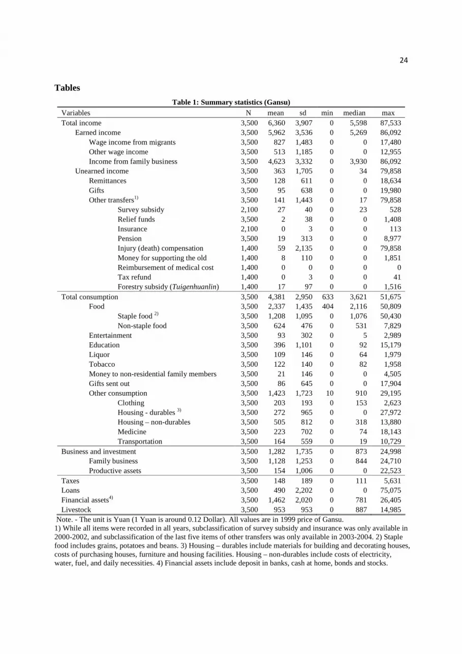
Table 1: Summary statistics (Gansu) Variables N mean sd min median max Total income 3,500 6,360 3,907 0 5,598 87,533 Earned income 3,500 5,962 3,536 0 5,269 86,092 Wage income from migrants 3,500 827 1,483 0 0 17,480 Other wage income 3,500 513 1,185 0 0 12,955 Income from family business 3,500 4,623 3,332 0 3,930 86,092 Unearned income 3,500 363 1,705 0 34 79,858 Remittances 3,500 128 611 0 0 18,634 Gifts 3,500 95 638 0 0 19,980 Other transfers1) 3,500 141 1,443 0 17 79,858 Survey subsidy 2,100 27 40 0 23 528 Relief funds 3,500 2 38 0 0 1,408 Insurance 2,100 0 3 0 0 113 Pension 3,500 19 313 0 0 8,977 Injury (death) compensation 1,400 59 2,135 0 0 79,858 Money for supporting the old 1,400 8 110 0 0 1,851 Reimbursement of medical cost 1,400 0 0 0 0 0 Tax refund 1,400 0 3 0 0 41 Forestry subsidy (Tuigenhuanlin) 1,400 17 97 0 0 1,516 Total consumption 3,500 4,381 2,950 633 3,621 51,675 Food 3,500 2,337 1,435 404 2,116 50,809 Staple food 2) 3,500 1,208 1,095 0 1,076 50,430 Non-staple food 3,500 624 476 0 531 7,829 Entertainment 3,500 93 302 0 5 2,989 Education 3,500 396 1,101 0 92 15,179 Liquor 3,500 109 146 0 64 1,979 Tobacco 3,500 122 140 0 82 1,958 Money to non-residential family members 3,500 21 146 0 0 4,505 Gifts sent out 3,500 86 645 0 0 17,904 Other consumption 3,500 1,423 1,723 10 910 29,195 Clothing 3,500 203 193 0 153 2,623 Housing - durables 3) 3,500 272 965 0 0 27,972 Housing – non-durables 3,500 505 812 0 318 13,880 Medicine 3,500 223 702 0 74 18,143 Transportation 3,500 164 559 0 19 10,729 Business and investment 3,500 1,282 1,735 0 873 24,998 Family business 3,500 1,128 1,253 0 844 24,710 Productive assets 3,500 154 1,006 0 0 22,523 Taxes 3,500 148 189 0 111 5,631 Loans 3,500 490 2,202 0 0 75,075 Financial assets4) 3,500 1,462 2,020 0 781 26,405 Livestock 3,500 953 953 0 887 14,985

Note. - The unit is Yuan (1 Yuan is around 0.12 Dollar). All values are in 1999 price of Gansu. 1) While all items were recorded in all years, subclassification of survey subsidy and insurance was only available in 2000-2002, and subclassification of the last five items of other transfers was only available in 2003-2004. 2) Staple food includes grains, potatoes and beans. 3) Housing – durables include materials for building and decorating houses, costs of purchasing houses, furniture and housing facilities. Housing – non-durables include costs of electricity, water, fuel, and daily necessities. 4) Financial assets include deposit in banks, cash at home, bonds and stocks.

25

Table 2: Summary statistics (Inner Mongolia) Variables N mean sd min median max Total income 4,000 9,716 5,972 357 8,626 70,047 Earned income 4,000 9,331 5,816 49 8,277 68,631 Wage income from migrants 4,000 328 1,146 0 0 17,349 Other wage income 4,000 669 1,429 0 0 12,687 Income from family business 4,000 8,334 5,676 0 7,308 68,631 Unearned income 4,000 329 990 0 64 22,444 Remittances 4,000 20 208 0 0 7,807 Gifts 4,000 119 834 0 0 22,388 Other transfers1) 4,000 190 483 0 56 10,815 Survey subsidy 2,400 48 52 0 56 741 Relief funds 4,000 1 22 0 0 672 Insurance 2,400 0 0 0 0 0 Pension 4,000 0 2 0 0 136 Injury (death) compensation 1,600 0 4 0 0 153 Money for supporting the old 1,600 4 75 0 0 2,056 Reimbursement of medical cost 1,600 0 3 0 0 117 Tax refund 1,600 3 34 0 0 718 Forestry subsidy (Tuigenhuanlin) 1,600 94 278 0 0 3,186 Total consumption 4,000 5,452 3,720 288 4,438 45,919 Food 4,000 2,297 885 105 2,171 8,817 Staple food 2) 4,000 838 402 0 787 4,438 Non-staple food 4,000 884 481 0 835 8,100 Entertainment 4,000 134 338 0 32 8,227 Education 4,000 630 1,329 0 154 13,713 Liquor 4,000 135 143 0 94 1,467 Tobacco 4,000 136 141 0 101 2,430 Money sent to non-residential family members 4,000 86 747 0 0 25,563 Gifts sent out 4,000 312 1,110 0 54 27,529 Other consumption 4,000 1,961 2,492 12 1,218 38,795 Clothing 4,000 346 342 0 265 5,016 Housing – durables 3) 4,000 270 1,247 0 0 28,346 Housing – non-durables 4,000 504 579 0 367 10,453 Medicine 4,000 327 999 0 92 21,465 Transportation 4,000 410 996 0 95 21,842 Business and investment 4,000 4,090 4,414 0 2,836 62,242 Family business 4,000 3,415 3,264 0 2,580 58,057 Productive assets 4,000 673 2,679 0 0 45,008 Taxes 4,000 349 482 0 201 7,964 Loans 4,000 1,404 3,358 0 0 63,800 Financial assets4) 4,000 2,784 3,357 2 1703 33,646 Livestock 4,000 1,285 3,948 0 694 61,763

Note. - The unit is Yuan (1 Yuan is around 0.12 Dollar). All values are in 1999 price of Inner Mongolia. 1) While all items were recorded in all years, subclassification of survey subsidy and insurance was only available in 2000-2002, and subclassification of the last five items of other transfers was only available in 2003-2004. 2) Staple food includes grains, potatoes and beans. 3) Housing – durables include materials for building and decorating houses, costs of purchasing houses, furniture and housing facilities. Housing – non-durables include costs of electricity, water, fuel, and daily necessities. 4) Financial assets include deposit in banks, cash at home, bonds and stocks.

26

Table 3: Average unearned and earned income in each group Unearned

income<median 1) Unearned income>median

Gansu Avg. unearned 32 (1,127) 810 (1,080) Unearned < Earned Avg. earned 6,040 (1,127) 6,415 (1,080) Avg. unearned 50 (1) 7,627 (47) Unearned > Earned Avg. earned 7 (1) 3,076 (47)

Inner Mongolia

Avg. unearned 66 (1,308) 833 (1,286) Unearned < Earned Avg. earned 9,191 (1,308) 10,145 (1,286) Avg. unearned NA (0) 6,922 (23) Unearned > Earned Avg. earned NA (0) 3,596 (23)

Note. – The number of observations in each group is in the bracket. 1) “Median” is the median of unearned income of all observations from the province with non-zero unearned income.

Table 4: Descriptive statistics of the control variables variables explanation N1) mean sd min max

Gansu Business household Dummy:=1 if household is a business

household; 0 if not 3,500 0.07 0.26 0 1

Rural cadres' household Dummy:=1 if household is a cadres' household; 0 if not

3,500 0.07 0.25 0 1

Household size Size of the household 3,500 4.77 1.34 0 10 Female labor ratio Female 16<=age<=60/household labor 3,500 0.48 0.15 0 1 Dependency ratio (household size - member

16<=age<=60)/member 16<=age<=60 3,500 0.29 0.21 0 1

Gender household head Dummy:=1 if gender of household head is male; 0 if not

3,497 1.00 0.06 0 1

Age household head Age of household head 3,497 41.88 11.10 5 83 Education level household head

Years of education 3,486 6.85 3.66 0 16

No. of disabled people No. of disabled people 16<=age<=60 3,500 0.07 0.29 0 3 Inner Mongolia Business household Dummy:=1 if household is a business

household; 0 if not 4,000 0.03 0.18 0 1

Rural cadres' household Dummy:=1 if household is a cadres' household; 0 if not

4,000 0.04 0.19 0 1

Household size Size of the household 4,000 3.72 0.98 1 8 Female labor ratio Female 16<=age<=60/household labor 4,000 0.48 0.15 0 1 Dependency ratio (household size - member

16<=age<=60)/member 16<=age<=60 4,000 0.22 0.20 0 1

Gender household head Dummy:=1 if gender of household head is male; 0 if not

3,995 0.99 0.09 0 1

Age household head Age of household head 3,995 44.10 8.89 23 78 Education level household head

Years of education 3,995 8.25 2.50 0 16

No. of disabled people No. of disabled people 16<=age<=60 4,000 0.08 0.40 0 4 1) Based on all 5 survey rounds in 2000-2004. The difference in the number of observations is due to missing values.

27

Table 5: Regressions results - Consumption Consumption (exclusive gifts given) Gansu Inner Mongolia OLS FE PT OLS FE PT Panel 1: Living expenditures (full sample) Unearned permanent income 0.473*** 0.319** (0.081) (0.116) Unearned (transitory) income 0.465*** 0.436*** 0.471*** 0.327*** 0.339*** 0.334*** (0.082) (0.076) (0.081) (0.068) (0.070) (0.075) Earned permanent income 0.390*** 0.244*** (0.035) (0.025) Earned (transitory) income 0.252*** 0.155*** 0.146*** 0.194*** 0.124*** 0.133*** (0.041) (0.042) (0.041) (0.019) (0.025) (0.023) Loans 0.277*** 0.240*** 0.275*** 0.193*** 0.197*** 0.188*** (0.075) (0.062) (0.072) (0.043) (0.044) (0.042) Unearned (permanent) = Earned (permanent) 1) 0.013 0.001 0.329 0.061 0.003 0.533 Unearned transitory = Earned transitory 0.000 0.009 R-squared 0.601 0.466 0.616 0.436 0.292 0.442 N. of Obs. 2,788 2,788 2,788 3,196 3,196 3,196 Panel 2: Living expenditures (exclusive observations with Unearned income >>Earned income) Unearned permanent income 0.614*** 0.459** (0.091) (0.156) Unearned (transitory) income 0.616*** 0.582*** 0.644*** 0.473*** 0.545*** 0.493*** (0.092) (0.105) (0.094) (0.133) (0.139) (0.137) Earned permanent income 0.393*** 0.242*** (0.035) (0.025) Earned (transitory) income 0.254*** 0.158*** 0.147*** 0.192*** 0.121*** 0.130*** (0.042) (0.044) (0.042) (0.019) (0.025) (0.023) Loans 0.273*** 0.236*** 0.270*** 0.192*** 0.196*** 0.186*** (0.074) (0.061) (0.071) (0.043) (0.044) (0.043) Unearned (permanent) = Earned (permanent) 1) 0.000 0.000 0.021 0.038 0.003 0.176 Unearned transitory = Earned transitory 0.000 0.009 R-squared 0.604 0.470 0.620 0.436 0.295 0.442 N. of Obs. 2,753 2,753 2,753 3,176 3,176 3,176

Note. – Time varying village dummies are included in all regressions. Financial assets, livestock as specified in equations (8)-(10), and variables in Table 4 are included in all regressions. Robust standard errors are shown in brackets. 1) P-values from Wald test of equality of the coefficients. *, **, *** Significant at the 10%, 5%, 1% levels.

28

Table 6: Regression results – Investment and savings

Gansu Inner Mongolia OLS FE PT OLS FE PT Business and investment L.Unearned permanent income 0.064 0.048 (0.047) (0.150) L.Unearned (transitory) income 0.039 -0.042 0.039 0.001 0.008 -0.005 (0.044) (0.047) (0.040) (0.064) (0.071) (0.077) L.Earned permanent income 0.259*** 0.527*** (0.049) (0.053) L.Earned (transitory) income 0.095** 0.004 -0.025 0.284*** -0.032 -0.023 (0.043) (0.021) (0.040) (0.031) (0.068) (0.048) Loans 0.269*** 0.291*** 0.251*** 0.471*** 0.478*** 0.425*** (0.054) (0.050) (0.051) (0.082) (0.088) (0.077) Unearned (permanent) = Earned (permanent) 0.318 0.357 0.003 0.000 0.714 0.005 Unearned transitory = Earned transitory 0.245 0.851 R-squared 0.502 0.465 0.542 0.533 0.402 0.601 N. of Obs. 2,089 2,089 2,089 2,400 2,400 2,400 Saving in financial assets Unearned permanent income 0.225* -0.037 (0.120) (0.125) Unearned (transitory) income 0.279** 0.420** 0.304** 0.063 0.125 0.098 (0.129) (0.145) (0.132) (0.081) (0.091) (0.089) Earned permanent income 0.043 0.055** (0.030) (0.021) Earned (transitory) income 0.104*** 0.140** 0.150*** 0.076*** 0.109*** 0.106*** (0.031) (0.043) (0.043) (0.017) (0.029) (0.023) Loans -0.018 -0.015 -0.019 -0.024 -0.004 -0.022 (0.012) (0.015) (0.012) (0.022) (0.029) (0.022) Unearned (permanent) = Earned (permanent) 0.184 0.061 0.143 0.877 0.877 0.479 Unearned transitory = Earned transitory 0.256 0.932 R-squared 0.402 0.394 0.407 0.284 0.233 0.285 N. of Obs. 2,089 2,089 2,089 2,400 2,400 2,400 Panel 2: without observations with Unearned income >> Earned income

Business and investment L.Unearned permanent income 0.044 0.075 (0.091) (0.180) L.Unearned (transitory) income 0.009 0.000 0.020 -0.009 0.042 0.030 (0.094) (0.080) (0.089) (0.140) (0.152) (0.131) L.Earned permanent income 0.260*** 0.528*** (0.049) (0.054) L.Earned (transitory) income 0.094** 0.004 -0.027 0.284*** -0.032 -0.023 (0.043) (0.022) (0.040) (0.031) (0.069) (0.048) Loans 0.270*** 0.290*** 0.252*** 0.469*** 0.477*** 0.423*** (0.054) (0.050) (0.051) (0.082) (0.087) (0.076) Unearned (permanent) = Earned (permanent) 0.409 0.963 0.035 0.042 0.694 0.022 Unearned transitory = Earned transitory 0.644 0.716 R-squared 0.503 0.466 0.544 0.533 0.404 0.602 N. of Obs. 2,058 2,058 2,058 2,382 2,382 2,382

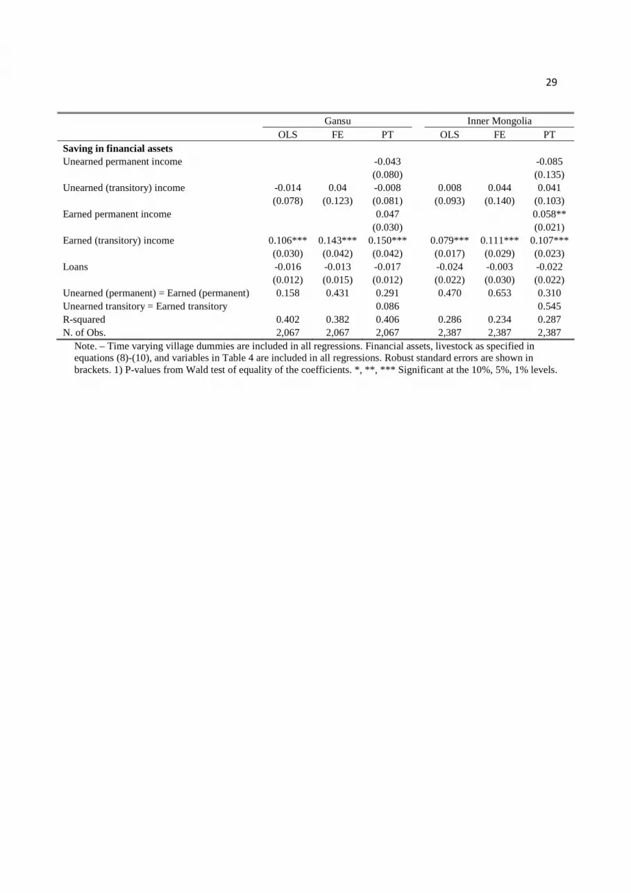
29

Gansu Inner Mongolia OLS FE PT OLS FE PT Saving in financial assets Unearned permanent income -0.043 -0.085 (0.080) (0.135) Unearned (transitory) income -0.014 0.04 -0.008 0.008 0.044 0.041 (0.078) (0.123) (0.081) (0.093) (0.140) (0.103) Earned permanent income 0.047 0.058** (0.030) (0.021) Earned (transitory) income 0.106*** 0.143*** 0.150*** 0.079*** 0.111*** 0.107*** (0.030) (0.042) (0.042) (0.017) (0.029) (0.023) Loans -0.016 -0.013 -0.017 -0.024 -0.003 -0.022 (0.012) (0.015) (0.012) (0.022) (0.030) (0.022) Unearned (permanent) = Earned (permanent) 0.158 0.431 0.291 0.470 0.653 0.310 Unearned transitory = Earned transitory 0.086 0.545 R-squared 0.402 0.382 0.406 0.286 0.234 0.287 N. of Obs. 2,067 2,067 2,067 2,387 2,387 2,387

Note. – Time varying village dummies are included in all regressions. Financial assets, livestock as specified in equations (8)-(10), and variables in Table 4 are included in all regressions. Robust standard errors are shown in brackets. 1) P-values from Wald test of equality of the coefficients. *, **, *** Significant at the 10%, 5%, 1% levels.

30

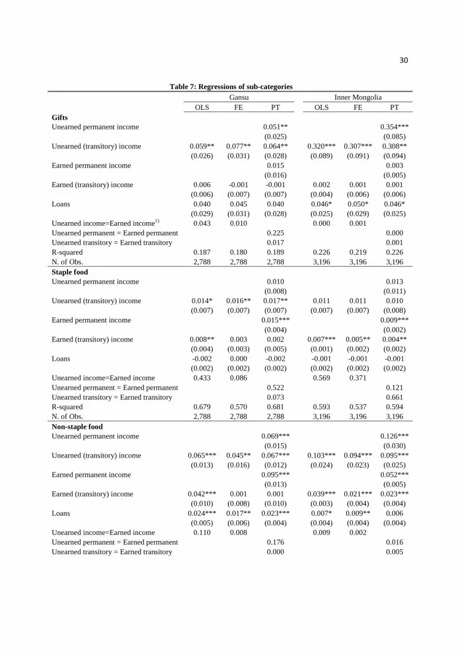
Table 7: Regressions of sub-categories Gansu Inner Mongolia OLS FE PT OLS FE PT Gifts Unearned permanent income 0.051** 0.354*** (0.025) (0.085) Unearned (transitory) income 0.059** 0.077** 0.064** 0.320*** 0.307*** 0.308** (0.026) (0.031) (0.028) (0.089) (0.091) (0.094) Earned permanent income 0.015 0.003 (0.016) (0.005) Earned (transitory) income 0.006 -0.001 -0.001 0.002 0.001 0.001 (0.006) (0.007) (0.007) (0.004) (0.006) (0.006) Loans 0.040 0.045 0.040 0.046* 0.050* 0.046* (0.029) (0.031) (0.028) (0.025) (0.029) (0.025) Unearned income=Earned income1) 0.043 0.010 0.000 0.001 Unearned permanent = Earned permanent 0.225 0.000 Unearned transitory = Earned transitory 0.017 0.001 R-squared 0.187 0.180 0.189 0.226 0.219 0.226 N. of Obs. 2,788 2,788 2,788 3,196 3,196 3,196 Staple food Unearned permanent income 0.010 0.013 (0.008) (0.011) Unearned (transitory) income 0.014* 0.016** 0.017** 0.011 0.011 0.010 (0.007) (0.007) (0.007) (0.007) (0.007) (0.008) Earned permanent income 0.015*** 0.009*** (0.004) (0.002) Earned (transitory) income 0.008** 0.003 0.002 0.007*** 0.005** 0.004** (0.004) (0.003) (0.005) (0.001) (0.002) (0.002) Loans -0.002 0.000 -0.002 -0.001 -0.001 -0.001 (0.002) (0.002) (0.002) (0.002) (0.002) (0.002) Unearned income=Earned income 0.433 0.086 0.569 0.371 Unearned permanent = Earned permanent 0.522 0.121 Unearned transitory = Earned transitory 0.073 0.661 R-squared 0.679 0.570 0.681 0.593 0.537 0.594 N. of Obs. 2,788 2,788 2,788 3,196 3,196 3,196 Non-staple food Unearned permanent income 0.069*** 0.126*** (0.015) (0.030) Unearned (transitory) income 0.065*** 0.045** 0.067*** 0.103*** 0.094*** 0.095*** (0.013) (0.016) (0.012) (0.024) (0.023) (0.025) Earned permanent income 0.095*** 0.052*** (0.013) (0.005) Earned (transitory) income 0.042*** 0.001 0.001 0.039*** 0.021*** 0.023*** (0.010) (0.008) (0.010) (0.003) (0.004) (0.004) Loans 0.024*** 0.017** 0.023*** 0.007* 0.009** 0.006 (0.005) (0.006) (0.004) (0.004) (0.004) (0.004) Unearned income=Earned income 0.110 0.008 0.009 0.002 Unearned permanent = Earned permanent 0.176 0.016 Unearned transitory = Earned transitory 0.000 0.005

31

Table 7 continued Gansu Inner Mongolia OLS FE PT OLS FE PT R-squared 0.664 0.557 0.691 0.537 0.379 0.545 N. of Obs. 2,788 2,788 2,788 3,196 3,196 3,196 Clothing Unearned permanent income 0.009** 0.008 (0.004) (0.012) Unearned (transitory) income 0.010** 0.012** 0.011** 0.020** 0.025** 0.025** (0.004) (0.006) (0.004) (0.010) (0.010) (0.010) Earned permanent income 0.014*** 0.024*** (0.002) (0.003) Earned (transitory) income 0.010*** 0.007** 0.007** 0.016*** 0.006** 0.006** (0.002) (0.002) (0.003) (0.002) (0.003) (0.003) Loans 0.004 0.005* 0.004 0.001 -0.001 0.000 (0.003) (0.002) (0.003) (0.002) (0.002) (0.002) Unearned income=Earned income 0.960 0.367 0.735 0.038 Unearned permanent = Earned permanent 0.234 0.189 Unearned transitory = Earned transitory 0.331 0.071 R-squared 0.456 0.293 0.459 0.346 0.171 0.361 N. of Obs. 2,788 2,788 2,788 3,196 3,196 3,196 Housing- durables Unearned permanent income 0.149** 0.024 (0.055) (0.057) Unearned (transitory) income 0.152** 0.137** 0.154** 0.037 0.046* 0.042 (0.051) (0.046) (0.050) (0.027) (0.024) (0.030) Earned permanent income 0.012 0.032** (0.010) (0.011) Earned (transitory) income 0.013 0.013 0.014 0.029*** 0.025** 0.026** (0.010) (0.011) (0.013) (0.008) (0.010) (0.010) Loans 0.042 0.052 0.042 0.058** 0.061** 0.058** (0.030) (0.033) (0.030) (0.023) (0.023) (0.023) Unearned income=Earned income 0.007 0.008 0.784 0.403 Unearned permanent = Earned permanent 0.013 0.895 Unearned transitory = Earned transitory 0.007 0.595 R-squared 0.241 0.214 0.241 0.182 0.153 0.182 N. of Obs. 2,788 2,788 2,788 3,196 3,196 3,196 Housing - non-durables Unearned permanent income 0.037** 0.018 (0.014) (0.021) Unearned (transitory) income 0.039** 0.049** 0.040** 0.006 0.002 0.002 (0.014) (0.020) (0.015) (0.010) (0.009) (0.012) Earned permanent income 0.053*** 0.028*** (0.013) (0.005) Earned (transitory) income 0.058** 0.064** 0.062** 0.025*** 0.019** 0.020*** (0.018) (0.024) (0.023) (0.005) (0.006) (0.006) Loans 0.028** 0.024** 0.028** 0.020** 0.023** 0.020** (0.010) (0.010) (0.010) (0.006) (0.007) (0.006) Unearned income=Earned income 0.265 0.522 0.094 0.131

32

Table 7 continued Gansu Inner Mongolia OLS FE PT OLS FE PT Unearned permanent = Earned permanent 0.309 0.646 Unearned transitory = Earned transitory 0.305 0.166 R-squared 0.500 0.456 0.500 0.353 0.211 0.354 N. of Obs. 2,788 2,788 2,788 3,196 3,196 3,196 Medicine Unearned permanent income 0.015 0.038 (0.015) (0.045) Unearned (transitory) income 0.014 0.021 0.015 0.042 0.047 0.044 (0.014) (0.014) (0.013) (0.034) (0.029) (0.034) Earned permanent income 0.020 0.003 (0.014) (0.008) Earned (transitory) income 0.010 0.003 0.002 -0.001 -0.009 -0.005 (0.011) (0.012) (0.012) (0.005) (0.008) (0.007) Loans 0.051 0.052 0.051 0.053** 0.057** 0.053** (0.035) (0.038) (0.035) (0.018) (0.017) (0.018) Unearned income=Earned income 0.790 0.323 0.231 0.078 Unearned permanent = Earned permanent 0.785 0.451 Unearned transitory = Earned transitory 0.453 0.174 R-squared 0.157 0.122 0.158 0.169 0.167 0.169 N. of Obs. 2,788 2,788 2,788 3,196 3,196 3,196 Transportation Unearned permanent income 0.055** 0.068** (0.024) (0.031) Unearned (transitory) income 0.052** 0.038 0.050** 0.047** 0.038* 0.040* (0.022) (0.024) (0.022) (0.018) (0.020) (0.021) Earned permanent income 0.034** 0.042*** (0.011) (0.006) Earned (transitory) income 0.026** 0.019** 0.019* 0.037*** 0.028*** 0.030*** (0.009) (0.008) (0.010) (0.005) (0.006) (0.007) Loans 0.027** 0.027** 0.026** 0.020** 0.021** 0.020** (0.011) (0.012) (0.012) (0.008) (0.009) (0.008) Unearned income=Earned income 0.256 0.461 0.573 0.626 Unearned permanent = Earned permanent 0.409 0.419 Unearned transitory = Earned transitory 0.172 0.625 R-squared 0.233 0.178 0.234 0.237 0.194 0.238 N. of Obs. 2,788 2,788 2,788 3,196 3,196 3,196 Entertainment Unearned permanent income 0.012 -0.003 (0.008) (0.011) Unearned (transitory) income 0.012 0.013 0.012 0.003 0.006 0.005 (0.008) (0.011) (0.009) (0.007) (0.007) (0.007) Earned permanent income 0.009** 0.008*** (0.004) (0.002) Earned (transitory) income 0.008** 0.007* 0.007 0.005** 0.003 0.003 (0.004) (0.004) (0.005) (0.002) (0.002) (0.002) Loans 0.000 0.000 0.000 0.005** 0.004 0.004**

33

Table 7 continued Gansu Inner Mongolia OLS FE PT OLS FE PT (0.002) (0.003) (0.002) (0.002) (0.002) (0.002) Unearned income=Earned income 0.660 0.647 0.706 0.713 Unearned permanent = Earned permanent 0.709 0.348 Unearned transitory = Earned transitory 0.647 0.733 R-squared 0.205 0.173 0.205 0.206 0.163 0.207 N. of Obs. 2,788 2,788 2,788 3,196 3,196 3,196 Education Unearned permanent income 0.074* -0.019 (0.040) (0.047) Unearned (transitory) income 0.065* 0.065 0.064 0.012 0.022 0.024 (0.039) (0.040) (0.040) (0.033) (0.025) (0.036) Earned permanent income 0.140*** 0.036*** (0.026) (0.008) Earned (transitory) income 0.078*** 0.036** 0.031 0.029*** 0.021** 0.021** (0.019) (0.015) (0.031) (0.007) (0.008) (0.009) Loans 0.098** 0.060** 0.097** 0.030** 0.028** 0.029** (0.044) (0.026) (0.043) (0.011) (0.010) (0.011) Unearned income=Earned income 0.751 0.498 0.614 0.967 Unearned permanent = Earned permanent 0.156 0.262 Unearned transitory = Earned transitory 0.473 0.942 R-squared 0.269 0.177 0.284 0.193 0.149 0.194 N. of Obs. 2,788 2,788 2,788 3,196 3,196 3,196 Liquor Unearned permanent income 0.010** 0.030** (0.004) (0.009) Unearned (transitory) income 0.009** 0.005** 0.008** 0.028*** 0.027*** 0.027*** (0.003) (0.003) (0.003) (0.007) (0.005) (0.007) Earned permanent income 0.010*** 0.006*** (0.002) (0.001) Earned (transitory) income 0.006** 0.003* 0.003 0.005*** 0.002** 0.003** (0.002) (0.001) (0.002) (0.001) (0.001) (0.001) Loans 0.004** 0.004*** 0.004** 0.001 0.002 0.001 (0.002) (0.001) (0.002) (0.001) (0.001) (0.001) Unearned income=Earned income 0.334 0.322 0.000 0.000 Unearned permanent = Earned permanent 0.830 0.015 Unearned transitory = Earned transitory 0.086 0.000 R-squared 0.550 0.502 0.554 0.379 0.378 0.382 N. of Obs. 2,788 2,788 2,788 3,196 3,196 3,196 Tobacco Unearned permanent income 0.013** 0.024** (0.006) (0.011) Unearned (transitory) income 0.014** 0.012** 0.014** 0.025** 0.026** 0.026** (0.005) (0.004) (0.005) (0.010) (0.010) (0.010) Earned permanent income 0.010*** 0.005*** (0.002) (0.001) Earned (transitory) income 0.005** 0.001 0.001 0.005*** 0.003*** 0.004***

34

Table 7 continued Gansu Inner Mongolia OLS FE PT OLS FE PT (0.002) (0.001) (0.002) (0.001) (0.001) (0.001) Loans 0.005*** 0.004** 0.005*** 0.001 0.002* 0.001 (0.001) (0.002) (0.001) (0.001) (0.001) (0.001) Unearned income=Earned income 0.094 0.010 0.043 0.024 Unearned permanent = Earned permanent 0.523 0.094 Unearned transitory = Earned transitory 0.012 0.031 R-squared 0.546 0.499 0.554 0.336 0.304 0.337 N. of Obs. 2,788 2,788 2,788 3,196 3,196 3,196 Family business L.Unearned permanent income 0.056* 0.113 (0.033) (0.128) L.Unearned (transitory) income 0.031 -0.045 0.026 -0.053 -0.108* -0.106* (0.029) (0.036) (0.027) (0.046) (0.056) (0.060) L.Earned permanent income 0.198*** 0.438*** (0.039) (0.034) L.Earned (transitory) income 0.085** 0.006 0.004 0.248*** 0.000 0.008 (0.038) (0.020) (0.036) (0.024) (0.048) (0.034) Loans 0.220*** 0.238*** 0.208*** 0.110** 0.046 0.073** (0.063) (0.061) (0.062) (0.034) (0.034) (0.029) Unearned income=Earned income 0.202 0.215 0.000 0.164 Unearned permanent = Earned permanent 0.004 0.016 Unearned transitory = Earned transitory 0.584 0.096 R-squared 0.537 0.475 0.569 0.543 0.304 0.634 N. of Obs. 2,089 2,089 2,089 2,400 2,400 2,400 Investment in productive assets L.Unearned permanent income 0.009 -0.063 (0.024) (0.116) L.Unearned (transitory) income 0.009 0.002 0.013 0.055 0.117** 0.102* (0.022) (0.022) (0.021) (0.042) (0.054) (0.055) L.Earned permanent income 0.062** 0.088** (0.023) (0.030) L.Earned (transitory) income 0.010 -0.003 -0.028 0.035** -0.030 -0.031 (0.012) (0.009) (0.018) (0.017) (0.029) (0.026) Loans 0.049 0.052 0.043 0.362*** 0.433*** 0.353*** (0.031) (0.033) (0.031) (0.074) (0.089) (0.074) Unearned income=Earned income 0.978 0.839 0.686 0.025 Unearned permanent = Earned permanent 0.115 0.226 Unearned transitory = Earned transitory 0.148 0.044 R-squared 0.215 0.188 0.232 0.450 0.437 0.458 N. of Obs. 2,089 2,089 2,089 2,400 2,400 2,400 Note. – Time varying village dummies are included in all regressions. Financial assets, livestock as specified in equation (15), and variables in Table 4 are included in all regressions. Robust standard errors are shown in brackets. 1) P-values from Wald test of equality of the coefficients. * Significant at the 10% level. ** Significant at the 5% level. *** Significant at the 1% level.

35

Table 8: Regression results with percentiles of income per capita Gansu Inner Mongolia OLS FE OLS FE Living expenditures Unearned income poorest 25 percentiles 0.064 0.301** 0.204 0.306 (0.145) (0.147) (0.299) (0.322) Unearned income middle 50 percentiles 0.346*** 0.416*** 0.491** 0.626*** (0.094) (0.108) (0.160) (0.165) Unearned income top 25 percentiles 0.433*** 0.400*** 0.274*** 0.265*** (0.098) (0.086) (0.066) (0.064) Earned income poorest 25 percentiles 0.021 0.029 0.066 0.026 (0.089) (0.086) (0.061) (0.068) Earned income middle 50 percentiles 0.133** 0.064 0.159*** 0.096** (0.057) (0.058) (0.032) (0.038) Earned income top 25 percentiles 0.227*** 0.147** 0.188*** 0.124*** (0.041) (0.045) (0.022) (0.028) Loans poorest 25 percentiles 0.444*** 0.343** 0.349** 0.336** (0.123) (0.129) (0.113) (0.121) Loans middle 50 percentiles 0.383** 0.356** 0.191** 0.194** (0.138) (0.133) (0.065) (0.063) Loans top 25 percentiles 0.227** 0.195*** 0.153** 0.156** (0.075) (0.057) (0.050) (0.054) Bottom p25: Unearned = Earned1) 0.748 0.049 0.641 0.386 Middle 50p: Unearned = Earned 0.012 0.000 0.039 0.002 Top 25p: Unearned = Earned 0.041 0.006 0.210 0.039 R-squared 0.609 0.477 0.441 0.300 N. of Obs. 2,788 2,788 3,196 3,196 Business and investment L.Unearned income poorest 25 percentiles 0.006 0.113 0.181 0.213 (0.113) (0.123) (0.315) (0.360) L.Unearned income middle 50 percentiles 0.013 -0.009 0.028 -0.026 (0.072) (0.086) (0.119) (0.147) L.Unearned income top 25 percentiles 0.027 -0.064 -0.035 0.002 (0.055) (0.056) (0.072) (0.080) L.Earned income poorest 25 percentiles 0.057 -0.028 0.150** -0.147 (0.084) (0.041) (0.072) (0.136) L.Earned income middle 50 percentiles 0.073 -0.007 0.217*** -0.052 (0.057) (0.027) (0.042) (0.089) L.Earned income top 25 percentiles 0.089* 0.004 0.252*** -0.036 (0.046) (0.022) (0.033) (0.075) Loans poorest 25 percentiles 0.360** 0.467** 0.169 0.256** (0.135) (0.150) (0.114) (0.120) Loans middle 50 percentiles 0.088** 0.128** 0.355*** 0.376*** (0.043) (0.055) (0.091) (0.104) Loans top 25 percentiles 0.284*** 0.298*** 0.650*** 0.646*** (0.062) (0.057) (0.096) (0.098) Bottom p25: Unearned = Earned 0.635 0.259 0.920 0.292 Middle 50p: Unearned = Earned 0.336 0.981 0.120 0.867

36

Table 8 continued Gansu Inner Mongolia OLS FE OLS FE Top 25p: Unearned = Earned 0.355 0.271 0.000 0.757 R-squared 0.508 0.476 0.549 0.420 N. of Obs. 2,089 2,089 2,400 2,400 Saving in financial assets Unearned income poorest 25 percentiles 0.231 0.329 0.421 0.615 (0.161) (0.280) (0.305) (0.454) Unearned income middle 50 percentiles 0.297** 0.535** 0.048 0.114 (0.119) (0.163) (0.134) (0.182) Unearned income top 25 percentiles 0.275* 0.395** 0.046 0.092 (0.158) (0.176) (0.091) (0.101) Earned income poorest 25 percentiles 0.021 0.031 -0.042 -0.060 (0.088) (0.112) (0.059) (0.079) Earned income middle 50 percentiles 0.111** 0.155** 0.055* 0.046 (0.052) (0.064) (0.032) (0.044) Earned income top 25 percentiles 0.102** 0.141** 0.068*** 0.094** (0.035) (0.048) (0.021) (0.031) Loans poorest 25 percentiles 0.137** 0.216*** -0.013 0.005 (0.055) (0.056) (0.086) (0.105) Loans middle 50 percentiles 0.005 -0.026 -0.006 0.030 (0.043) (0.058) (0.024) (0.031) Loans top 25 percentiles -0.035* -0.033** -0.052 -0.051 (0.018) (0.016) (0.035) (0.045) Bottom p25: Unearned = Earned 0.210 0.334 0.140 0.153 Middle 50p: Unearned = Earned 0.109 0.013 0.959 0.708 Top 25p: Unearned = Earned 0.281 0.165 0.822 0.989 R-squared 0.406 0.402 0.286 0.237 N. of Obs. 2,089 2,089 2,400 2,400

Note. – Time varying village dummies are included in all regressions. Financial assets, livestock as specified in equations (8)-(10), and variables in Table 4 are included in all regressions. Robust standard errors are shown in brackets. The 25th percentile of income per capita is 876 Yuan and 1599 Yuan in Gansu and Inner Mongolia respectively. The 75th percentile of income per capita is 1677 Yuan and 3378 Yuan in Gansu and Inner Mongolia respectively. 1) P-values from Wald test of equality of the coefficients. * Significant at the 10% level. ** Significant at the 5% level. *** Significant at the 1% level.

37

Table 9: Regression results with female labor ratio Gansu Inner Mongolia OLS FE OLS FE Living expenditures Unearned income 0.386** 0.485** 0.593** 0.684** (0.190) (0.191) (0.217) (0.225) Unearned income*female labor ratio 16<=age<=60 0.151 -0.108 -0.480 -0.626* (0.369) (0.376) (0.344) (0.352) Earned income 0.295*** 0.259** 0.163*** 0.146** (0.069) (0.086) (0.046) (0.061) Earned income*female labor ratio 16<=age<=60 -0.094 -0.226 0.063 -0.048 (0.123) (0.162) (0.085) (0.106) Loans 0.161 0.033 0.140 0.197* (0.176) (0.157) (0.111) (0.119) Loans*female labor ratio 16<=age<=60 0.261 0.465 0.109 -0.003 (0.460) (0.409) (0.224) (0.233) Ratio=p25: Unearned income=Earned income1) 0.030 0.001 0.035 0.005 Ratio=p75: Unearned income=Earned income 0.012 0.000 0.037 0.001 R-squared 0.601 0.470 0.437 0.294 N. of Obs. 2,788 2,788 3,196 3,196 Business and investment L.Unearned income -0.041 -0.324** -0.351 0.197 (0.072) (0.123) (0.284) (0.256) L.Unearned income*female labor ratio 16<=age<=60 0.164 0.576** 0.627 -0.339 (0.113) (0.210) (0.458) (0.431) L.Earned income 0.192** 0.109* 0.297*** -0.18 (0.069) (0.059) (0.076) (0.131) L.Earned income*female labor ratio 16<=age<=60 -0.199** -0.205** -0.025 0.311* (0.096) (0.096) (0.122) (0.176) Loans -0.300* -0.333** 0.515** 0.627*** (0.158) (0.158) (0.173) (0.175) Loans*female labor ratio 16<=age<=60 1.217*** 1.338*** -0.091 -0.29 (0.322) (0.329) (0.330) (0.304) Ratio=p25: Unearned income=Earned income 0.138 0.037 0.004 0.352 Ratio=p75: Unearned income=Earned income 0.348 0.348 0.000 0.643 R-squared 0.521 0.498 0.534 0.408 N. of Obs. 2,089 2,089 2,400 2,400 Saving in financial assets Unearned income 0.146 0.129 0.335 0.445 (0.175) (0.252) (0.270) (0.393) Unearned income*female labor ratio 16<=age<=60 0.271 0.587 -0.490 -0.575 (0.370) (0.532) (0.452) (0.655) Earned income 0.144** 0.239** 0.060 0.067 (0.060) (0.091) (0.045) (0.070) Earned income*female labor ratio 16<=age<=60 -0.086 -0.216 0.033 0.087 (0.108) (0.167) (0.083) (0.133) Loans -0.026 -0.01 -0.069 0.024

38

Table 9 continued Gansu Inner Mongolia OLS FE OLS FE (0.068) (0.096) (0.079) (0.116) Loans*female labor ratio 16<=age<=60 0.018 -0.007 0.089 -0.059 (0.142) (0.202) (0.148) (0.215) Ratio=p25: Unearned income=Earned income 0.227 0.114 0.451 0.409 Ratio=p75: Unearned income=Earned income 0.168 0.044 0.868 0.652 R-squared 0.402 0.396 0.284 0.233 N. of Obs. 2,089 2,089 2,400 2,400

Note. – Time varying village dummies are included in all regressions. Financial assets, livestock as specified in equations (8)-(10), and variables in Table 4 are included in all regressions. Robust standard errors are shown in brackets. The 25th and 75th percentiles of female labor ratio in Gansu are 0.4 and 0.5 respectively. In Inner Mongolia they are 0.33 and 0.5 respectively. 1) P-values from Wald test of equality of the coefficients. * Significant at the 10% level. ** Significant at the 5% level. *** Significant at the 1% level.

39

Table 10: Regression results with big unearned income and big loans

Gansu Inner Mongolia OLS FE OLS FE Living expenditures Unearned income 0.282* 0.414** 0.705** 0.331 (0.176) (0.188) (0.247) (0.294) Big unearned income 0.185 0.024 -0.378 0.010 (0.168) (0.176) (0.242) (0.288) Earned income 0.257*** 0.158*** 0.195*** 0.124*** (0.040) (0.042) (0.019) (0.025) Loans 0.593*** 0.330*** 0.308*** 0.229*** (0.078) (0.080) (0.040) (0.044) Big loans -0.338*** -0.095 -0.128** -0.034 (0.102) (0.094) (0.054) (0.059) Unearned income = Earned income1) 0.886 0.170 0.038 0.478 R-squared 0.606 0.467 0.439 0.293 N. of Obs. 2,788 2,788 3,196 3,196 Family business and investment L.Unearned income 0.102 0.014 -0.111 0.091 (0.161) (0.267) (0.311) (0.416) L.Big unearned income -0.065 -0.057 0.120 -0.078 (0.161) (0.251) (0.303) (0.404) L.Earned income 0.095** 0.004 0.284*** -0.031 (0.043) (0.021) (0.031) (0.068) Loans 0.198*** 0.279*** 0.318*** 0.380*** (0.056) (0.063) (0.067) (0.068) Big loans 0.077 0.012 0.168* 0.103 (0.075) (0.073) (0.091) (0.095) Unearned income = Earned income 0.963 0.970 0.211 0.780 R-squared 0.502 0.465 0.535 0.403 N. of Obs. 2,089 2,089 2,400 2,400 Saving in financial assets Unearned income 0.087 0.243 -0.045 0.509 (0.211) (0.308) (0.313) (0.453) Big unearned income 0.195 0.178 0.108 -0.383 (0.199) (0.284) (0.298) (0.439) Earned income 0.102*** 0.139** 0.076*** 0.110*** (0.030) (0.042) (0.017) (0.029) Loans -0.126* -0.024 -0.034 -0.019 (0.067) (0.098) (0.050) (0.074) Big loans 0.117* 0.010 0.012 0.017 (0.068) (0.099) (0.052) (0.076) Unearned income = Earned income 0.948 0.746 0.701 0.377 R-squared 0.403 0.394 0.284 0.233 N. of Obs. 2,089 2,089 2,400 2,400

Note. Time varying village dummies are included in all regressions. Financial assets, livestock as specified in equations 8 and 9, and variables in Table 4 are included in all regressions. Robust standard errors are shown in brackets. “Big” means bigger than the 90th percentile of non-zero observations in the province. 1) P-values from Wald test of equality of the coefficients. * Significant at the 10% level. ** Significant at the 5% level. *** Significant at the 1% level.

40

Figure 1: Consumption decision in each category, where

.400=,9.0=,)05.0+1(=)(,1.0/=)( 21.0 uIβxxfxxu