Transition Point Displacement Control on a Wing Equipped with Actuators

American Institute of Aeronautics and Astronautics

1

Transition point displacement control on a wing equipped with actuators

M. Labib1, A. V. Popov2, J. Fays3 and R. M. Botez4

École de technologie supérieure, Montréal, Québec, Canada, H3C 1K3

The main objective of the global project is to develop a system for active control of wing airfoil geometry during flight in order to allow the drag reduction. In-flight modification of aircraft wing airfoils will make possible the maintenance of laminar flow over the wing as flight regime changes and therefore will allow reductions in fuel consumption. Drag reduction on a wing can be achieved by modifications in the laminar to turbulent flow transition point position, which should move toward the trailing edge of the airfoil wing. As the transition point plays a crucial part in this project, this article focuses on the control of its position on the airfoil, as well as the deflection control on a morphing wing airfoil equipped with actuators, sensors and flexible skin. The reference airfoil is the laminar WTEAT-TE1 airfoil on which a flexible skin is located from 7% to 65% of the chord. This airfoil is modified by use of a single point control (at 36% of the chord), where is assumed that one actuator acts, thus creating a deflection from -2 cm to +2 cm. The values of the chord percentage, Mach number, angle of attack and deflection allow us to calculate the pressure and the transition point position at each step. A number of pressure coefficients values are collected by use of optical sensors and sent to the controller acting on the wing airfoil. The real time controller should then determine the transition point position only from the pressure coefficient distributions versus the airfoil chord, and send the appropriate command to the actuator so that the transition points can move towards the trailing edge. The inputs that vary are the deflections and the angle of attack. As they both change, the transition point position also moves accordingly. A model of a Shape Memory Alloy (SMA) has been carried out in Matlab/Simulink environment. The challenge is hence to realize the control with a SMA in the closed loop, as it has a non-linear behaviour. Several controllers, such as a PID controller, a proportional controller and variables gains (which are functions of deflections) are therefore necessary to control the SMA and the entire closed loop. Three simulations have been carried out to validate the control. The first simulation has the angle of attack constant and is performed for successive deflections. The second simulation has also different steps for the deflection but adds a sinusoidal component for the angle of attack, so that we get closer to a cruise flight regime. The third simulation has both the angle of attack and the deflection modeled as a sin wave. The outputs (the deflection and the transition point position) are well controlled and results are very good. We hence concluded that this method of control is suitable for the control of the transition point position on a morphing wing airfoil.

Nomenclature A = Ampere F = Applied force on the SMA i = Current in the SMA IMC = Internal Model Control °K = Kelvin K = Static gain of the PID

1M.Sc.A student, [email protected], AIAA Member 2 PhD student, [email protected], AIAA Member 3 Internship student, [email protected], AIAA Member 4 Professor, [email protected], AIAA Member

mailto:[email protected]





2

Kc = Critical gain of the PID Kd = Derivative gain of the PID Ki = Integral gain of the PID Kp = Proportional gain of the PID M = Mach number PID = Proportional Integral Derivative controller Re = Reynolds number SMA = Shape Memory Alloy Tc = Critical period of the SMA model TF = Transfer function Ti = Initial temperature in the SMA ZN = Ziegler and Nichols τc = Controller delay of the PID controlling the SMA model τ1 = Time delay of the PID controlling the SMA model τ2 = Time delay of the PID controlling the SMA model θ = Dead time of the PID controlling the SMA model

I. Introduction Due to fossil energy rarefaction, increases in fuel prices are burning issues. Moreover, global warming

prevention and increasing exploitation costs represent the main challenges in the aeronautical field. In the aerospace industry, these goals may be achieved by fuel consumption reduction, translated in drag reduction, and in most efficient wing design. To achieve this design, there is the need to obtain a larger part of the laminar flow on the wing, which is equivalent to the transition point displacement towards the trailing edge. Two different types of bibliographical research were realized: the first bibliographical research type concerned the existing literature on laminar flow improvement on a wing, while the second bibliographical research type concerned the Shape Memory Alloy (SMA) existing applications on a wing.

One method of laminar flow improvement study comprises wing geometry modification by inflating and

deflating installed bumps at a certain frequency. Munday et al [1] used piezoelectric actuators to inflate and deflate bumps on the upper surface of wings in a wind tunnel to determine the transition point displacement. Turbulent flow was thus delayed and the lift coefficient was increased by up to 7%. The flow active control was therefore achieved by modifying the wing geometry.

Another laminar flow study method concerned wing geometry modification by installation and optimization of a

bump on the upper surface of the airfoil to improve shock wave control in transonic flow [2]. Optimization of this bump gave a 70% reduction of friction drag and a 15% reduction of the total drag on the wing. Since bump optimization required a high number of iterations during numerical aerodynamic analysis, the Euler-2D code with a boundary layer correction was chosen to save time. Flow around the optimized wing geometry was studied using a Navier-Stokes code.

Sobieczky and Geissler [3] simulated the behavior of a wing configured with one bump at the leading edge and a

second bump at the trailing edge of the upper surface for Mach numbers ranging from 0.72 to 0.77. Results show a drag reduction of 10%.

Yet another method is the modification of the geometry by leading and trailing edge variations. Martins and

Catalano [4] studied drag reduction on adaptive wings for a transport aircraft manufactured by Embraer Aircraft Company. The camber of the adaptive wing airfoil was modified to deform the leading and the trailing edge of the airfoil. The panel method with a boundary layer correction was used. The transition point moved at 40 % from the airfoil chord (instead of 10 %), and the friction drag was reduced by 24 %.

Powers et al. [5] performed various flight tests at the NASA Dryden Flight Research Center on an F-111 aircraft.

Their results were useful for numerical aerodynamics code validation and showed an increase in the lift coefficient dependent on wing airfoil geometry modification.


3

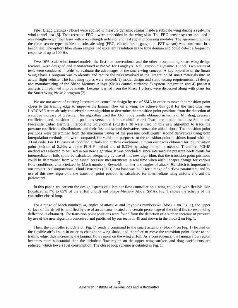
Fiber Bragg gratings (FBGs) were applied to measure dynamic strains inside a subscale wing during a real-time wind tunnel test [6]. Two recoated FBG’s were embedded in the wing skin. The FBG sensor system included a wavelength-swept fiber laser with a wavelength indicator and fast signal processing modules. The agreement among the three sensor types inside the subscale wing (FBG, electric strain gauge and PZT sensor) was confirmed in a bench test. The optical fiber strain sensors had excellent resolution in the time domain and could detect a frequency response of up to 100 Hz.

Two 16% scale wind tunnel models, the first one conventional and the other incorporating smart wing design

features, were designed and manufactured at NASA for Langley's 16 ft Transonic Dynamic Tunnel. Two series of tests were conducted in order to evaluate the advantages of the smart wing concept. A key objective of the Smart Wing Phase 1 program was to identify and reduce the risks involved in the integration of smart materials into an actual flight vehicle. The following topics were studied: 1) model design and static testing requirements; 2) design and manufacturing of the Shape Memory Alloys (SMA) control surfaces; 3) system integration and 4) post-test analysis and planned improvements. Lessons learned from the Phase 1 efforts were discussed along with plans for the Smart Wing Phase 2 program [7].

We are not aware of existing literature on controller design by use of SMA in order to move the transition point

closer to the trailing edge to improve the laminar flow on a wing. To achieve this goal for the first time, our LARCASE team already conceived a new algorithm to determine the transition point positions from the detection of a sudden increase of pressure. This algorithm used the Xfoil code results obtained in terms of lift, drag, pressure coefficients and transition point positions versus the laminar airfoil chord. Two interpolation methods: Spline and Piecewise Cubic Hermite Interpolating Polynomial (PCHIP) [8] were used in this new algorithm to trace the pressure coefficients distributions, and their first and second derivatives versus the airfoil chord. The transition point positions were determined from the maximum values of the pressure coefficients’ second derivatives using both interpolation methods and were compared, for validation purposes, to the transition point positions found with the XFoil code. For 119 cases of modified airfoils and airflow conditions, a mean error was obtained for the transition point position of 0.23% with the PCHIP method and of 0.33% by using the spline method. Therefore, PCHIP method was selected to be used in our new algorithm. It was concluded, since intermediate pressure coefficients for intermediate airfoils could be calculated adequately by use of this new algorithm, that the transition point positions could be determined from wind tunnel pressure measurements in real time when airfoil shapes change for various flow conditions, characterized by Mach numbers, Reynolds number and angles of attack [9], which is important in our project. A Computational Fluid Dynamics (CFD) data base was built for a range of airflow parameters, and by use of this new algorithm, the transition point position is calculated for intermediate wing airfoils and airflow parameters.

In this paper, we present the design aspects of a laminar flow controller on a wing equipped with flexible skin

(localized at 7% to 65% of the airfoil chord) and Shape Memory Alloy (SMA). Fig. 1 shows the scheme of the controller closed loop.

For a range of Mach numbers M, angles of attack α and Reynolds numbers Re (block 1 on Fig. 1), the upper

surface of the airfoil is modified by use of an actuator located at a certain percentage of the chord (its corresponding deflection is obtained). The transition point positions were found from the detection of a sudden increase of pressure by use of the new algorithm conceived and published by our team in [8] and shown in the block 2 on Fig. 1.

Then, the controller (block 3 on Fig. 1) sends a command to the smart actuators (block 4 on Fig. 1) located on

the flexible airfoil skin in order to change the wing shape, and therefore to move the transition point closer to the trailing edge, thus increasing the laminar flow region on the wing airfoil. As a consequence, the laminar flow region becomes more substantial than the turbulent flow region on the upper wing surface, and drag coefficients are reduced, which lowers fuel consumption. The closed loop scheme is detailed in Fig. 1:

Figure 1. Controller closed loop scheme

The reference airfoil considered in this paper is the laminar WTEAT-TE1 airfoil, with its chord of 50 cm. The

airfoil coordinates and its data expressed in terms of lift, drag, pressure coefficients and transition point position versus the chord were validated numerically and experimentally by IAR-NRC.

This reference airfoil is modified by use of a single control point localized at 36% of the chord, where is

assumed that one actuator acts, thus creating a deflection from -2 cm to +2 cm of the upper surface airfoil. Seventeen different airfoils are thus obtained by LAMSI team, and are visually shown on Fig. 2:

Figure 2. WTEAT-TE1 reference airfoil and its modified airfoils shapes

Varaa is the name of the series of modified airfoils created from the laminar WTEAT-TE1 airfoil. Here is the

nomenclature:

Table 1. Airfoil names and their associated deflections Airfoil name varaa-3 varaa-2 varaa-1 varaa1 varaa2 varaa3 varaa4 varaa5

Deflection (mm) +20 +16 +10 +8 +5 +3 +1.5 +0.5

Name of airfoil varaa6 varaa7 varaa8 varaa9 varaa10 varaa11 varaa12 varaa13 Deflection (mm) -0.5 -1.5 -3 -5 -8 -10 -16 -20

The controller simulation and validation is here performed for the following airflow conditions: angles of attack

α = -2° to +2°, Reynolds number Re = 2.29*106 and Mach number M = 0.2. These airflow conditions correspond to the cruise subsonic flight regime at low angles of attack. It is also considered that one actuator (or control point) acts at the airfoil chord percentage of 36% in order to deflect its airfoil upper surface, and therefore to modify its shape.


4

II. Closed loop controller design The controller goal mainly concerns the displacement of the transition point position closer to the trailing edge,

in order to produce a higher laminar flow region on the airfoil, and therefore to control the airfoil deflection for all airflow conditions. The closed loop is composed of three main blocks, as shown on Fig. 1:

- ‘Determination of pressure and transition point position’, block 2 - ‘Update of pressure and transition point position values’, block 5 - ‘SMA’, block 4 - ‘Controller’, block 3 Each block is detailed in the following sub-sections.

A. Block 2: ‘Determination of pressure and transition point position’ The block 2 receives the values of the four inputs (shown in block 1 on Fig. 1) and calculates the values of

pressure coefficients versus the chord and transition point positions for airflow conditions with the new algorithm recently conceived at LARCASE, and summarized in the introduction of the paper as described in [9].

Figure 3. Details of block 2: ‘Determination of the pressure coefficients versus the chord and transition

point position’ [9]

B. Block 5: ‘Update of pressure and transition point position values’ The ‘Update of pressure and transition point position values’ block (block 5 on Fig. 1) is the same as block 2.

We still have in input of bock 5 the angle of attack, the Mach number and the percentage of chord. The difference with block 2 is that we now have the new value of the deflection. In block 2, we had the deflection as defined in input. In block 5, we have the actual deflection calculated in output of the ‘SMA’ block. Block 5 hence realizes an update of the pressure and the transition point position. We therefore have the actual pressure and the actual transition point position at each step of the simulation.


5

C. Block 4: ‘SMA’ The ‘SMA block’ contains the model of the Shape Memory Alloy (SMA), as shown on the following figure:

Figure 4. Details of block 4: ‘SMA’

The goal of block 4 is to control the airfoil deflection located at 36% of the airfoil chord, created with a SMA.

The PID controller sends a command to the SMA, in order to change the airfoil shape, so that the transition point can move towards the trailing edge. One goal of this PID controller is to control the airfoil deflection (its modified shape), while its other goal is to control the displacement of the transition point position to obtain the same value of the transition point displacement (following the control application) as the value of the initial transition point displacement.

The SMA model was conceived by LAMSI team, more specifically by Dr Patrick Terriault, and the PID

controller was conceived by LARCASE team. The SMA model is shown on Fig. 5:


6

Figure 5. The SMA model scheme

The three inputs of this model are: the initial temperature Ti = 380 °K (see Fig. 6), the current intensity i of the SMA and the applied force F on the SMA. The model outputs are: the final temperature, the SMA displacement at 36% of the chord corresponding to the airfoil deflection and the SMA phase variation with temperature, as seen on Fig. 6. An SMA has a non-linear behaviour [10], due to the several phases characterizing its functioning, as shown on the following Fig. 6:

Figure 6. SMA cycle

In our paper here presented, a PID controller is designed to control the SMA. The SMA has an initial unchanged behaviour. In order to act accurately, the SMA needs to go initially through the transformation phase, and further through the cooling phase. Before these two phases, the control can not be realized, due to the intrinsic behaviour of the SMA. The SMA can behave correctly only following these two phases, as seen on results shown in Paragraph III.


7

Two methods are used to design the PID controller: The Ziegler and Nichols (ZN) method and The Internal Model Control (IMC) method. These methods are described in the next two subsections II.C.1 and II.C.2.

1. Ziegler and Nichols ZN method [11]


8

This method allows us to determine a satisfactory value for each of the three gains (Kp, Ki and Kd) present in the PID controller. Kp is the proportional gain, Ki is the integral gain and Kd is the derivative gain. The methodology to obtain the values of the three gains is next described.

In order to find the values of Kp, Ki and Kd, the first step is to determine the values of the critical gain Kc and the

oscillating period T . We therefore set Kc i and Kd to zero and we only use Kp. We increase Kp until the output starts to oscillate. When the output starts to oscillate, it means that we have found the critical gain Kc. We measure the value of K , as well as the period of oscillations T . c c

The second step is to use the values of K and T to find the correct values of Kc c p, Ki and Kd. The following relationships are used to determine these gains [11] :

0.6 ; 2 ;8

p cp c i d p

c

K TK K K K KT

= = = (1)

We obtain Kp = 171, Ki = 6.22 and Kd = 1175.60. The displacement of the actuator versus the temperature is shown on Fig. 7, while the displacement of the

actuator versus time is shown on Fig. 8.a).

300 320 340 360 380 400 4200.08

0.081

0.082

0.083

0.084

0.085

0.086

Temperature (K)

Dis

plac

emen

t of t

he a

ctua

tor (

m)

Figure 7. Displacement of the actuator versus

temperature with ZN method

0 500 1000 1500 2000 2500 3000 3500 4000 4500 50000.08

0.081

0.082

0.083

0.084

0.085

0.086

Time (s)

Dis

plac

emen

t of t

he a

ctua

tor (

m)

Ouput : Real DisplacementInput : Desired Displacement

Initialisation phase

Figure 8.a) Displacement of the actuator versus time with ZN method

The input is expressed as two successive steps as seen on Fig. 8.a). From t = 0 s to t = 1000 s, the input remains at 0.0801m. From t = 1000 s to t = 3000 s, the first step input goes from 0.0801 m to 0.0831 m. Then, from t = 3000 s to t = 5000 s, the second step input goes from 0.0831 m to 0.0822 m.

a) Initialisation phase This phase corresponds to the first 1000 seconds. We can see that the input and the output are not the same

during this period of time. This difference comes from the intrinsic behaviour of the SMA. Indeed, as seen on Fig. 6, the working point has to go through both transformation phase and cooling phase before the action of any control on the SMA. This period of time can not be avoided, and the control can not be achieved until the working point has reached the end of the cooling phase. Once this period of time is over, the control can act precisely and give satisfactory results. We found a precision of 0.12 % and a time response at 0.5 % of the input of 681 seconds.

The precision and the time response at 0.5 % of the input are calculated in this paragraph and in the following

ones, as explained underneath. The precision is defined as:

( )% *100Output Input

PrecisionInput

−= (2)

The time response at 0.5 % of the input is the time that takes the system to be stabilized at ± 0.5 % of the final value, which is the input here. To illustrate how this value is measured, we can see the following example. For the first step, the input corresponds to a displacement of the actuator from 0.0801m to 0.0831m. We can hence calculate 0.0831+0.0831*0.005 = 0.0835 and 0.0831-0.0831*0.005 = 0.0827. We plot the following equations: y = 0.0835 and y = 0.0827. The idea here is to find the moment when the output always remains between those two equations. This moment corresponds to the time response at 0.5% of the input, as shown on the following figure:


9

Figure 8.b) Measurement of the time response at 0.5 % of input

b) First step At t = 1000s, the input goes from 0.0801m to 0.0831m. We found a precision of 0.02 % and a time response at

0.5 % of the input of 374 seconds.

c) Second step At t = 3000s, the input goes from 0.0831 m to 0.0822 m. We found a precision of 0.03 % and a time response at

0.5 % of the input of 748 seconds. We summarize the precision and the time response at 0.5% of the input in the following table:

Table 2. Characteristics of the response by use of ZN method Desired displacement

Precision Time response at 0.5 % of input Initialisation phase 0.12% 681 s

First step 0.02% 374 s Second step 0.03% 748 s 2. Internal Model Control (IMC) method [12] The Internal Model Control (IMC) is another method to determine the values of the PID parameters. Two steps

are followed in order to use this method. During the first step, we have to obtain a second order transfer function


10

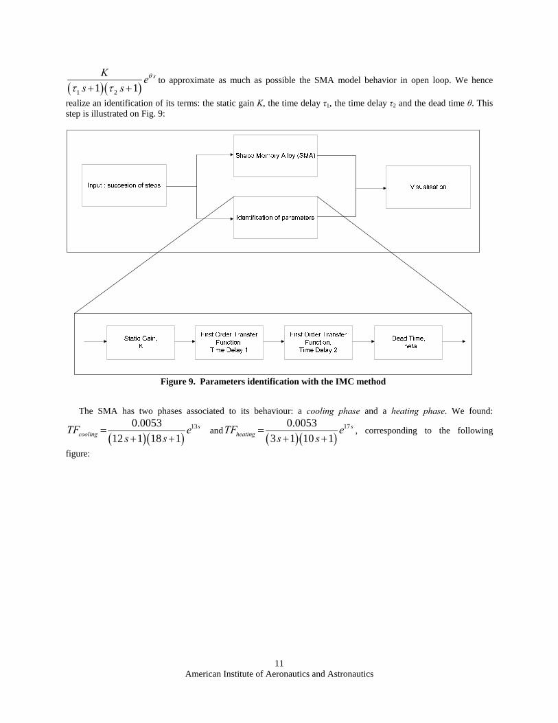
( )( )1 21 1sK e

s sθ

τ τ+ +to approximate as much as possible the SMA model behavior in open loop. We hence

realize an identification of its terms: the static gain K, the time delay τ1, the time delay τ2 and the dead time θ. This step is illustrated on Fig. 9:

Figure 9. Parameters identification with the IMC method

The SMA has two phases associated to its behaviour: a cooling phase and a heating phase. We found:

( )( )130.0053

12 1 18 1s

coolingTF es s

=+ + ( )( )

170.00533 1 10 1

sheatingTF e

s s=

+ + and , corresponding to the following

figure:


11

0 50 100 150 200 250 3000

5

10

15

Time (s)

Cur

rent

(A)

0 50 100 150 200 250 3000.08

0.082

0.084

0.086

0.088

Time (s)

Dis

plac

emen

t of t

he a

ctua

tor (

m)

Identification of parametersBehaviour of SMA model

Input : Current in the SMA

Cooling phase

Heating phase

Delays due to phase transformation

Figure 10. Current and actuator displacement versus time obtained with the IMC method


12

The second step of the IMC method is to evaluate the Kp, Ki and Kd gains by use of equations [12] in closed loop. We consider here the closed loop shown on Fig. 4, not the one shown on Fig. 1.

( ) ( ) ( )1 2 1 21; ;p i d

c c

K K KK K K c

τ τ τ τθ τ θ τ+

= = =+ +

θ τ+

(3)

We notice the presence of the new term τc (written as tau_c in Fig. 12.a) and Fig. 12.b)), which is the controller time delay, and is used in this method as an additional degree of freedom. We can modify its value to find the best control of the SMA model. The actuator displacement versus the temperature is shown on Fig. 11, while the actuator displacement versus time is shown on Fig. 12.a) for several values of τ . c

300 320 340 360 380 400 4200.08

0.081

0.082

0.083

0.084

0.085

0.086

Temperature (K)

Dis

plac

emen

t of t

he a

ctua

tor (

m)

Figure 11. Actuator displacement versus temperature with

IMC method

0 500 1000 1500 2000 2500 3000 3500 4000 4500 50000.08

0.081

0.082

0.083

0.084

0.085

0.086

Time (s)

Dis

plac

emen

t of t

he a

ctua

tor (

m)

Output : Real displacement for tauc = 0




Input : Desired displacement

Initialisation phases

Figure 12.a) Actuator displacement versus time with IMC method for several τc


13

We enforced the same successive steps as the ones used for the ZN method. We notice that the best value following different τ


14

c’s cases is the case where 0cτ = . We hence obtain Kp = 144.28, Ki = 11.10 and Kd = 332.96.

a) Initialisation phase

This phase corresponds to the first 1000 seconds. We can see that the input and the output are not the same during this period. The difference between them comes from the intrinsic behaviour of the SMA. Indeed, as seen on Fig. 6, the working point has to go through both transformation phase and cooling phase before the action of any SMA control. This phase can not be avoided, and the control can not be achieved until the working point reaches the end of the cooling phase. Once this period is over, the control can act precisely and give satisfactory results. We found a precision of 0.07 % and a time response at 0.5 % of the input of 297 seconds. The precision is here again calculated with Eq. (2).

b) First step

At t = 1000s, the input goes from 0.0801 m to 0.0831 m. We can notice a precision of 0.09 % and a time response at 0.5 % of the input of 208 seconds.

We can see on the following figure how the time responses at 0.5 % of the input are calculated:


c) Second step At t = 3000s, the input goes from 0.0831 m to 0.0822 m. We can notice a precision of 0.23 % and a time

response at 0.5 % of the input of 381 seconds. We summarize the precision and the time response at 0.5% of the input in the following Table 3:

Table 3. Characteristics of the response with IMC method Desired displacement Precision Time response at 0.5 % of input Initialisation phase 0.07% 297 s

First step 0.09% 208 s


15

3. Comparison of results obtained with both methods In order to choose between these two methods, we can compare on the same graph the obtained results:

It is clear that the parameters Kp, Ki and Kd found with IMC method for τc = 0 are better than the ones found with

ZN method. Even though the precision is a bit better with ZN method, the time response at 0.5 % of the input is by far better with the IMC method, as shown on Table 4. We therefore decided to use IMC method for the design of the PID controller.

Second step 0.23% 381 s

0 500 1000 1500 2000 2500 3000 3500 4000 4500 50000.08

0.081

0.082

0.083

0.084

0.085

0.086

Time (s)

Dis

plac

emen

t of t

he a

ctua

tor (

m)

Output : Real displacement with ZN methodOutput : Real displacement with IMC method for tauc = 0

Input : Desired displacement

Initialisation phases

Figure 13. Displacement of actuator versus time with methods ZN and IMC

Table 4. Comparison of desired displacement by use of ZN and IMC methods Desired displacement with ZN method Desired displacement with IMC method


16

4. Control improvement Even though the controller works properly, we decide to reduce the time response during the cooling phase.

Indeed, the controller designed with IMC method has a dead time θ, which creates a long time response, especially in the cooling phase. The idea here is to disconnect the controller action during the cooling phase, which physically means when the desired deflection is higher to the actual deflection. We disconnect the controller action with the instruction i = 0A in the SMA by use of the algorithm shown on Fig. 14:

The SMA responses improvements are shown on next Fig. 15 and 16.

Precision Time response Time response

at 0.5 % of input Precision at 0.5 % of input Initialisation phase 0.12% 681 s 0.07% 297 s

First step 0.02% 374 s 0.09% 208 s Second step 0.03% 748 s 0.23% 381 s

Figure 14. Algorithm for SMA control improvement

Figure 15. Displacement of the actuator versus temperature with the new algorithm

Figure 16.a) Displacement of the actuator versus time with the new algorithm


17

We can see on the following figure how the time responses at 0.5 % of the input are calculated:


We can see on Fig. 16.a) the improvement of the time response, while oscillations appear around the equilibrium

points. Following the first step, the time response at 0.5 % of the input is 44 seconds, instead of 208 seconds, and following the second step, the time response at 0.5 % of the input is 36 seconds, instead of 381 seconds as previously shown.

The oscillations which appear are caused by an inadequate evaluation of the current to enforce during the cooling

phase. Indeed, with a current of 0A, the sign of the quantity «desired deflection minus actual deflection» continuously changes. Therefore, we continuously switch in our algorithm (Fig. 14), thus creating oscillations.

Following several attempts on the current intensity value to be injected during the cooling phase, we decided to

enforce a 4A current during this phase, instead of 0A as previously. The obtained results are hence better, as seen on the following Fig. 17 and 18.a):


18

Figure 17. Displacement of the actuator versus temperature with the improved algorithm

Figure 18.a) Displacement of the actuator versus time with the improved algorithm

We can see on the following figure how the time response at 0.5 % of the input is calculated:


19


In this case, the oscillations around equilibrium point are much smaller, and the time responses are still

satisfactory. After the first step, we obtain a time response at 0.5 % of the input of 71 seconds, instead of 44 seconds previously, and after the second step, we obtain a time response at 0.5 % of the input of 52 seconds, instead of 36 seconds previously.

The SMA block (shown as block 4 on Fig. 1) is now well controlled. However, when this block is implemented

into the whole closed loop (see Fig. 1), the control is not satisfactory. For this reason, we need to implement a controller block before the SMA block in the closed loop (Fig. 1).

D. Block 3: ‘Controller’


20

The goal of this block is to control the airfoil deflection. It is located in the whole closed loop (Fig. 1), while the PID designed in the previous paragraph is only located in the SMA block.

Figure 19. Details of block 3: ‘Controller’

We have two types of closed loop dynamics (Fig. 1). On one hand, we have a very fast dynamics in block 2

(‘Determination of the pressure coefficients versus chord and transition point position’ block, see Fig. 3), with our real time algorithm which should react as fast as possible. On the other hand, we have in block 4 (‘SMA block’, see Fig. 4) a very slow dynamics, with very high time responses. For this reason, the PID controller located in the ‘SMA’ block is not capable of controlling the whole closed loop of Fig. 1. It was hence necessary to create a ‘Controller’ block located before the ‘SMA’ block in the closed loop, in order to deal with those two dynamics. This ‘Controller’ block is composed of two types of gains: a fixed proportional gain, and a variable gain. The proportional gain reduces the inertia of the system created by the SMA model. The variable gain adjusts the controller in function of the deflection value entered as input (block 1 on Fig. 1).

III Results and discussion Three different types of simulations were performed to validate the three controller design (two located in the

‘Controller’ block and one in the ‘SMA’ block), for the following airflow conditions: Mach number M = 0.2, Temperature T = 288.15 °K and Reynolds number Re = 2.29*106. The point where the actuator acts was located at 36% of the chord of the airfoil. Results obtained following these three types of simulations are represented and discussed in terms of airfoil deflections and transition point positions versus time in following sub-sections III.A, III.B and III.C. Three phases are present in these simulations, which are: initialization phase, first deflection and second deflection.

A. First simulation type

0During the first simulation, we consider the angle of attack � = 0 , while the airfoil deflection time variation is the following:

- From t = 0 s to t = 500 s, the deflection remains at 0 cm. - From t = 500 s to t = 1000 s, the deflection varies from 0 cm to 2 cm


21

- From t = 1000 s to t = 1500 s, the deflection varies from 2 to 1 cm Results are shown on Fig. 20.

Figure 20. First simulation type results

1. Initialization phase During the initialization phase, more precisely, during the first 500 seconds, the airfoil deflection input remains

at 0 cm. We can see that during the first 200 seconds period of time, the input is different from the output. During this time period of 200 seconds, the SMA has to go through both transformation phase and cooling phase (see Fig. 6). This time period can not be avoided, as is intrinsic to the SMA, and lasts actually 200 seconds. The control can not be achieved until the working point has reached the end of the cooling phase. Following this 200 seconds time period, it is seen that the transition point position and the airfoil deflection are well controlled, as both of them match well with the input. The transition point position was found to be at 31% of the chord by use of the transition point position algorithm (block 2 on Fig. 1). It was found a precision of 0.03 % for the airfoil deflection and of 0.04 % for the transition point position. The precision here and in the following paragraphs is seen as the relative error:

( )%Output Input

PrecisionInput

−=


22

*100 (4)

The time response at 5 % of the input is the time that takes the system to be stabilized at ± 5 % of the final value, which is the input here.

2. First airfoil deflection At t = 500 seconds, a deflection from 0 cm to 2 cm is enforced, which corresponds to the displacement of the

transition point position from 31% to 38% of the chord according to the algorithm described in the paper introduction [9]. The transition point and the deflection are controlled efficiently, as the time response is fast. Even

though there is an overshoot, the time response and the precision are satisfactory, for both the airfoil deflection and the transition point position (see Table 5). We found a precision of 0.5% for the airfoil deflection and of 0.02% for the transition point position. The time response at 5 % of the input is of 56 seconds for the deflection and of 57 seconds for the transition point position.

3. Second airfoil deflection At t = 1000 seconds, a second airfoil deflection from 2 cm to 1 cm is given, which corresponds to a displacement

of the transition point position between 38% and 33% of the chord according to [9]. The system time response and the precision are satisfactory. We obtained a precision of 4.7% for the deflection and 1.5% for the transition point position. The time response at 5 % of input is 47 seconds for the transition point position and 53 seconds for the airfoil deflection. We summarize the precision and the time response of the controlled quantities such as the airfoil deflection and the transition point position for all phases in the next Table 5:

Table 5. Characteristics of the responses during the first simulation Airfoil deflection Transition point position Precision Time response at 5 % of input Precision Time response at 5 % of input

Initialization phase 0.03% 200 s 0.04% 200 s First deflection 0.50% 56 s 0.02% 57 s

Second deflection 4.70% 53 s 1.50% 47 s

We can see in the following table that we succeeded in controlling the transition point position by changing the

shape of the airfoil:

Table 6. Variation of type of airfoil when transition point position changes


23

B. Second simulation type In this simulation, the angle of attack is modeled as a sinus function with 2° amplitude and with the frequency of

0.01 rad/sec, while the airfoil deflection varies with time as follows: - From t = 0 s to t = 500 s, the deflection remains at 0 cm - From t = 500 s to t = 1000 s, the deflection varies from 0 to 2 cm - From t = 1000 s to t = 1500 s, the deflection varies from 2 to 1 cm

Initialisation phase First deflection Second deflection From To From To From To

Airfoil name varaa0 varaa0 varaa0 varaa-3 varaa-3 varaa-1 Transition point position (% of chord) 31% 31% 31% 38% 38% 33%

The choice of the sin wave input for the angle of attack is justified by the fact that it corresponds to the small variations of the angle of attack around 0º, in the cruise regime, where the angle of attack may be continuously varying. The obtained results are shown on Fig. 21.

0 500 1000 1500-4

-2

0

2

4

Time (s)Def

lect

ion

of th

e ai

rfoil

(cm

)

0 500 1000 15000

0.2

0.4

0.6

0.8

Time (s)Tran

sitio

n po

int p

ositi

on (%

of c

hord

)

Time (s)Time (s)Time (s)

Output : Real deflection of the airfoilInput : Desired deflection of the airfoil

Output : Real transition point positionInput : Desired transition point position



Figure 21. Second simulation type results

It was found that the airfoil deflection is well controlled. The variation of the angle of attack in the second

simulation with respect to its variation in the first simulation does have no influence on the airfoil deflection control, as this airfoil deflection remains the same as during the first simulation. Only the transition point position oscillates and varies continuously due to the angle of attack sin wave variation.

1. Initialisation phase During the first 500 seconds, the input deflection remains at 0 cm. During this phase, the transition point position

(as output) does not fit its input, due to the non-linear behaviour of the SMA. After the 200 seconds of initialization, the transition point position control is well achieved. The position of the transition point varies very much from 7 % to 75 % of the airfoil chord; it fills the whole range of values accepted for the transition point. We found a precision of 0.03 % for the deflection and of 0.04 % for the transition point position.

2. First deflection At t = 500 seconds, a deflection from 0 cm to 2 cm is enforced. We can see on Fig. 21 a small overshoot. We

found the precision of 0.5 % for the airfoil deflection and of 0.12 % for the transition point position. The time response at 5 % of the input is 56 seconds for the airfoil deflection and is 47 seconds for the transition point position.


24

3. Second deflection At t = 1000 seconds, a deflection from 2 cm to 1 cm is given to the airfoil. We found a precision of 4.7% for the

airfoil deflection and of 0.02 % for the transition point position. The time response at 5% of the input is 53 seconds for the transition point position and 57 seconds for the transition point position. We summarize the precision and the time response of the controlled quantities such as the airfoil deflection and the transition point position for all phases in the next Table 7:

Table 7 Characteristics of the responses during the second simulation Airfoil deflection Transition point position Precision Time response at 5 % of input Precision Time response at 5 % of input

Initialisation phase 0.03% 200 s 0.04 % 200 s First deflection 0.50% 56 s 0.12 % 47 s

Second deflection 4.70% 53 s 0.02 % 57 s

C. Third simulation type The goal of this third simulation is to highlight that changing the shape of the airfoil allows us concretely to

move the transition point position towards the trailing edge. In this simulation, the angle of attack and the deflection are both modeled as sinus functions with 2° amplitude and with the frequency of 1

500 rad/sec. Results are shown on

Fig. 22.

0 500 1000 1500-4

-2

0

2

4

Time (s)

Def

lect

ion

of th

e ac

tuat

or (c

m)

0 500 1000 15000

0.2

0.4

0.6

0.8

Time (s)Tran

sitio

n po

int p

ositi

on (%

of c

hord

)

Input : Desired deflection of the airfoilOutput : Real deflection of the airfoil

Input : Desired transition point positionOutput : Real transition point position



Figure 22. Third simulation type results


25

We can notice here that the change of the shape of the airfoil allows us to move the transition point position towards the trailing edge. The principle of using a morphing wing airfoil equipped with actuators, sensors and flexible skin to reduce drag here works. The following two subsections describe in detail the results.

1. Initialization phase During this phase, the transition point position and the deflection do not fit the respective inputs, due to the non-

linear behaviour of the SMA. After the 200 seconds of initialization, both controls are well achieved. The transition point position control is well achieved, as well as the deflection. The position of the transition point varies from 15 % to 9 % of the chord. The deflection varies from 0.4 cm to 1.35 cm. The precision is here 1.07 % for the deflection and 1.03 % for the transition point position.

2. After the initialization phase During the next 1250 seconds, the control is satisfactory. The transition point position varies from 9 % to 76 %

of the chord, while the deflection varies from 1.35 cm to -0.15 cm. We find here a precision 0.94 % for the deflection and of 0.87 % for the transition point position. During all this phase, both responses are always located between ± 5 % of the input.

We can see on the following table how the airfoil changes its shape and the consequence on the position of the

transition point:

Table 8. Characteristics of the responses during the third simulation


26

IV Conclusions This article presents an easy implementing way of controlling the transition point position and the deflection on a

morphing wing airfoil equipped with actuators, sensors and flexible skin. The realization of the control has been carried out in two steps. The first step was to control the ‘SMA’ block (block 4 on Fig. 1). The SMA has a non-linear behaviour with a slow dynamics. The IMC method has been preferred to the ZN method as it provided better results. Once the closed loop inside the ‘SMA’ block has been controlled, we had to control the whole closed loop. The whole closed loop has a very fast dynamics, because of the real time controller located in the ‘Determination of the pressure coefficients versus chord and transition point position’ block (block 2 on Fig. 1). For this reason, a controller block (block 3 on Fig. 1) is necessary. The proportional gain reduces the inertia of the system created by

Name of the airfoil Transition point position (% of chord)

From To From To From To 0s 93s varaa2 varaa1 15% 13%

93s 157s varaa1 varaa-1 13% 11% 157s 358s varaa-1 varaa-2 11% 8% 358s 662s varaa-2 varaa-3 8% 7% 662s 1002s varaa-3 varaa-2 7% 16% 1002s 1205s varaa-2 varaa-1 16% 28% 1205s 1262s varaa-1 varaa1 28% 35% 1262s 1337s varaa1 varaa2 35% 46% 1337s 1391s varaa2 varaa3 46% 59% 1391s 1432s varaa3 varaa4 59% 70% 1432s 1451s varaa4 varaa5 70% 74% 1451s 1481s varaa5 varaa6 74% 75% 1481s 1500s varaa6 varaa7 75% 76%


27

the SMA model. The variable gain adjusts the control as function of the deflection value entered as input (block 1 on Fig. 1).

The simulations validated our choice of design, as we obtained fast and precise responses. The main advantage

of this method is its simplicity and its incorporation in experimental applications, such as in the controller of a morphing wing model.

Acknowledgements We would like to thank Dr Patrick Terriault (from LAMSI team) for the modeling of the Shape Memory Alloy

under Matlab/Simulink environment. We would also like to thank Dr Mahmoud Mamou and Dr Mahmood Khalid from the NSERC (National Sciences and Engineering Research Council) for the WTEA-TE1 airfoils modeling. We would like to thank Mr George-Henri Simon and Mr Philippe Molaret from Thales Avionics, and also Mr Eric Laurendeau from Bombardier Aeronautics for their collaboration on this paper.

We would like to thank aerospace companies Thales Avionics, Bombardier Aerospace and CRIAQ (Consortium of Research in the Aerospatial Industry in Quebec) for the funds that allowed the realization of this research as well as their collaboration in this work.

References [1] Munday, D., Jacob, J.D., T. Hauser, and Huang, G., 2002, Experimental and Numerical Investigation of Aerodynamic

Flow Control Using Oscillating Adaptive Surfaces, AIAA Paper No. 2002-2837, 1st AIAA Flow Control Conference, St. Louis. [2] Wadehn, W., Sommerer, A., Lutz, Th., Fokin, D., Pritschow, G., Wagner, S., 2002, Structural Concepts and

Aerodynamic Design of Shock Control Bumps, Proceedings 23nd ICAS Congress, Toronto, Canada, September 8 - 13, 2002, ICAS Paper 66R1.1

[3] Sobieczky, H., Geissler, W., 1999, Active Flow Control Based On Transonic Design Concepts , DLR German Aerospace Research Establishment, AIAA 99-3127.

[4] Martins, A. L., Catalano, F. M., 2003, Drag Optimisation For Transport Aircraft Mission Adaptive Wing, Journal of the Brazilian Society of Mechanical Sciences, vol. 25, no. 1, 2003.

[5] Powers, S.G. and Lannie D. Webb, 1997, Flight Wing Surface Pressure and Boundary-Layer Data Report from the F-111 Smooth Variable-Camber Supercritical Mission Adaptive Wing, Dryden Flight Research Center, Edwards, California, NASA Technical Memorandum 4789.

[6] Lee-Jung-Ryul et al., 2003, In-flight health monitoring of a subscale wing using a fibre Bragg grating sensor system, Smart Materials and Structures, v 12(1), p 147-155.

[7] Martin, C.A. et al., 1999, Design and fabrication of Smart Wing wind tunnel model and SMA control surfaces, Proceedings of the 1999 Smart Structures and Materials - Industrial and Commercial Applications of Smart Structures Technologies, Mar 2-Mar 4 1999, Newport Beach, CA, USA.

[8] Fritsch, F. N.; Carlson, R. E., 1980, Monotone piecewise cubic interpolation, SIAM J. Numer. Anal. 17 (1980), no. 2, 238-246.

[9] Popov A., Botez R.M., Labib, M., 2007 Transition point detection from the surface pressure distribution for controller design, AIAA Journal of Aircraft, in press.

[10] Song G., Kelly B., Agrawal BN., 2000, Active position control of a shape memory alloy wire actuated composite beam, Smart Materials & Structures 9 (5): 711-716, Oct 2000.

[11] Ziegler JG., Nichols NB., 1942, Optimum settings for automatic controllers, Transactions on ASME 1942; 64(8):759–768.

[12] Rivera DE., Morari M., Skogestad S., 1986, Internal Model Control. 4. PID Controller Design, Ind. Eng. Chem. Process Des. Dev., 25, 252-265.

Documents

Transition Point Displacement Control on a Wing Equipped with Actuators