Embed Size (px)
Citation preview
Southeast Michigan Council of Governments
TRAVEL TIME DATA COLLECTION
Technical Report
Prepared by:
MIDWESTERN CONSULTING, LLC
3815 Plaza Drive Ann Arbor, MI 48108
http://www.ms2soft.com
DEPARTMENT OF CIVIL AND ENVIRONMENTAL ENGINEERING
November 2008

(This page is intentionally left blank)
Table of Contents
Executive Summary..................................................................................................................................... i 1 Introduction............................................................................................................................................1 2 State-of-the-Practice Review ................................................................................................................2
2.1 General Guideline Documents.....................................................................................................2 2.2 Documents from State Departments of Transportation and Local Agencies ..............................3
3 Data Collection Methods.......................................................................................................................5 3.1 Test Vehicle Techniques .............................................................................................................5 3.2 Probe Vehicle Techniques...........................................................................................................7 3.3 Traffic Sampling Techniques .......................................................................................................8 3.4 Recommended Techniques.........................................................................................................9
4 Selection of Data Collection Periods.................................................................................................10 4.1 Periods for Congestion Characterization...................................................................................10 4.2 Periods for Free-flow Travel Time Characterization..................................................................10 4.3 Invalidating Factors....................................................................................................................10
5 Factors Affecting Sampling Activities...............................................................................................11 5.1 Coefficients of Variation of Travel Times...................................................................................11 5.2 Allowable Error ..........................................................................................................................12 5.3 Confidence Level .......................................................................................................................13 5.4 Need for Data Collection Across Several Days.........................................................................14 5.5 Absolute Minimum Number of Runs to Execute........................................................................17 5.6 Recommended Approach..........................................................................................................17
6 Selection of Survey Corridors and Study Segments .......................................................................18 6.1 Definition of Geographic Boundary............................................................................................18 6.2 Selection of a Network Stratification..........................................................................................18 6.3 Identification of Corridors...........................................................................................................19 6.4 Segmentation of Corridors.........................................................................................................19 6.5 Number of Segments to Survey ................................................................................................20 6.6 Segment/Corridor Selection.......................................................................................................21 6.7 Recommended Approach..........................................................................................................22 6.8 Recommended Regional Travel Time Monitoring Program ......................................................23
7 Determination of Number of Runs .....................................................................................................29 7.1 Coefficient of Variation Approach ..............................................................................................29 7.2 Average Range in Running Speed Approach............................................................................32 7.3 Recommended Approach..........................................................................................................33
8 Data Validation.....................................................................................................................................36 8.1 Sources of Error.........................................................................................................................36 8.2 Methods for Identifying Erroneous Data Points .........................................................................39
8.2.1 Visual Inspection ........................................................................................................39 8.2.2 Relative Inconsistency in Speed/Position Changes ...................................................39 8.2.3 Validation of Acceleration/Deceleration Rates ...........................................................39
8.3 Spot Data Correction Methods ..................................................................................................40 8.3.1 Data Removal.............................................................................................................41 8.3.2 Data Trimming ............................................................................................................41 8.3.3 Simple Average Data Replacement ...........................................................................41 8.3.4 Weighted Average Data Replacement .......................................................................42
8.4 Data Smoothing Techniques .....................................................................................................43 8.4.1 Simple Moving Average..............................................................................................44 8.4.2 Simple Exponential Smoothing ..................................................................................46 8.4.3 Kernel Smoothing .......................................................................................................47 8.4.4 Robust Smoothing Methods .......................................................................................49
8.5 Recommended Data Validation Method....................................................................................50 9 Data Storage Issues ............................................................................................................................52 10 Congestion Assessment and Reporting ...........................................................................................53
10.1 Congestion Assessment Parameters ........................................................................................53 10.2 Reporting Practice .....................................................................................................................55 10.3 Recommended Data Reporting .................................................................................................60
11 Estimation of Travel Time Parameters ..............................................................................................61 11.1 Cumulative Traveled Distance...................................................................................................61 11.2 Vehicle Acceleration Rates........................................................................................................62 11.3 Free Flow Speed .......................................................................................................................62 11.4 Average Speed ..........................................................................................................................62 11.5 Running Speed ..........................................................................................................................64 11.6 Number of Stops........................................................................................................................65 11.7 Segment Delay ..........................................................................................................................66 11.8 Stopped Delay ...........................................................................................................................67 11.9 Control Delay .............................................................................................................................68 11.10 Approach Delay.......................................................................................................................70
12 Data Collection.....................................................................................................................................71 12.1 Study Corridors..........................................................................................................................71
12.1.1 Segments .................................................................................................................73 12.2 Data Collection Method .............................................................................................................74
12.2.1 Training .....................................................................................................................74 12.2.2 Equipment .................................................................................................................74 12.2.3 Method ......................................................................................................................76
12.3 Data Processing ........................................................................................................................78 12.4 Results .......................................................................................................................................83
12.4.1 Travel Time Analysis Report Example (I – 75) .........................................................84 13 Appendix A – Term Glossary..............................................................................................................91 14 References ...........................................................................................................................................92
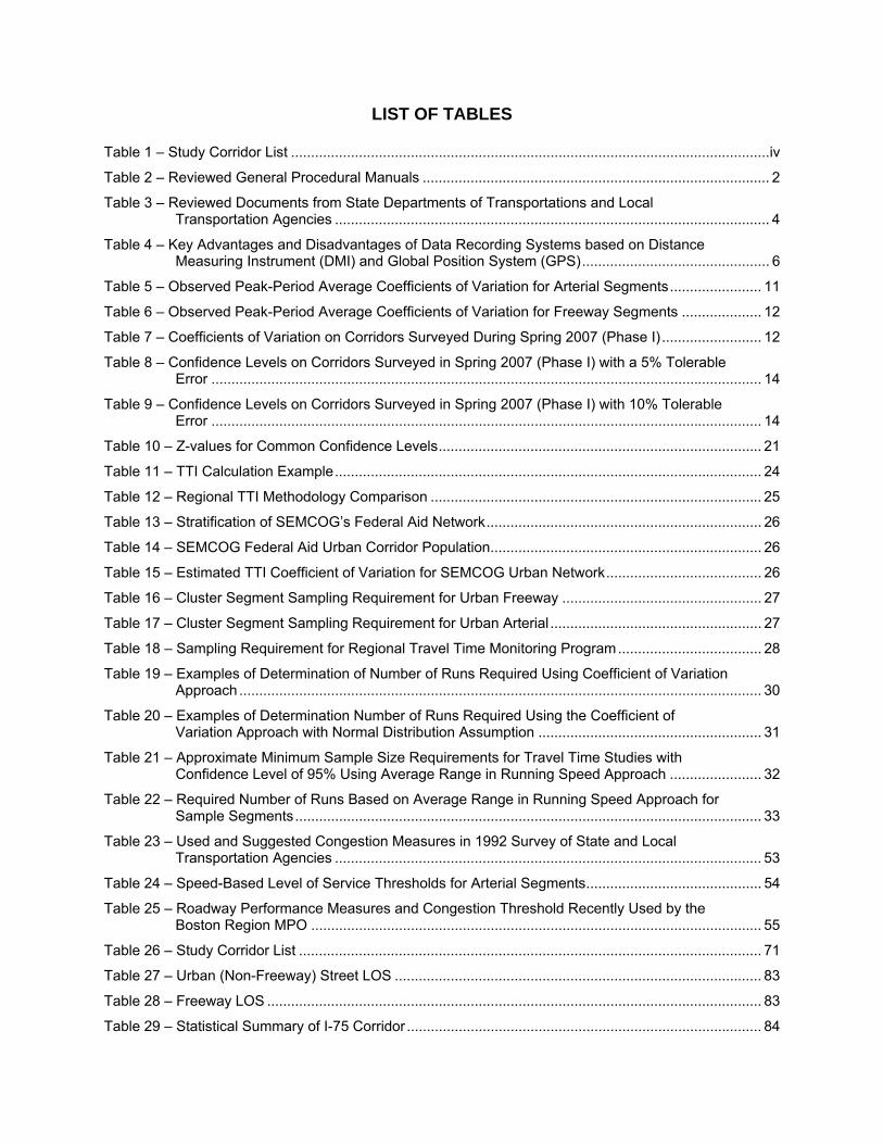
LIST OF TABLES
Table 1 – Study Corridor List ........................................................................................................................iv Table 2 – Reviewed General Procedural Manuals ....................................................................................... 2 Table 3 – Reviewed Documents from State Departments of Transportations and Local
Transportation Agencies ............................................................................................................. 4 Table 4 – Key Advantages and Disadvantages of Data Recording Systems based on Distance
Measuring Instrument (DMI) and Global Position System (GPS)............................................... 6 Table 5 – Observed Peak-Period Average Coefficients of Variation for Arterial Segments....................... 11 Table 6 – Observed Peak-Period Average Coefficients of Variation for Freeway Segments .................... 12 Table 7 – Coefficients of Variation on Corridors Surveyed During Spring 2007 (Phase I)......................... 12 Table 8 – Confidence Levels on Corridors Surveyed in Spring 2007 (Phase I) with a 5% Tolerable
Error .......................................................................................................................................... 14 Table 9 – Confidence Levels on Corridors Surveyed in Spring 2007 (Phase I) with 10% Tolerable
Error .......................................................................................................................................... 14 Table 10 – Z-values for Common Confidence Levels................................................................................. 21 Table 11 – TTI Calculation Example........................................................................................................... 24 Table 12 – Regional TTI Methodology Comparison ................................................................................... 25 Table 13 – Stratification of SEMCOG’s Federal Aid Network..................................................................... 26 Table 14 – SEMCOG Federal Aid Urban Corridor Population.................................................................... 26 Table 15 – Estimated TTI Coefficient of Variation for SEMCOG Urban Network....................................... 26 Table 16 – Cluster Segment Sampling Requirement for Urban Freeway .................................................. 27 Table 17 – Cluster Segment Sampling Requirement for Urban Arterial ..................................................... 27 Table 18 – Sampling Requirement for Regional Travel Time Monitoring Program.................................... 28 Table 19 – Examples of Determination of Number of Runs Required Using Coefficient of Variation
Approach ................................................................................................................................... 30 Table 20 – Examples of Determination Number of Runs Required Using the Coefficient of
Variation Approach with Normal Distribution Assumption ........................................................ 31 Table 21 – Approximate Minimum Sample Size Requirements for Travel Time Studies with
Confidence Level of 95% Using Average Range in Running Speed Approach ....................... 32 Table 22 – Required Number of Runs Based on Average Range in Running Speed Approach for
Sample Segments..................................................................................................................... 33 Table 23 – Used and Suggested Congestion Measures in 1992 Survey of State and Local
Transportation Agencies ........................................................................................................... 53 Table 24 – Speed-Based Level of Service Thresholds for Arterial Segments............................................ 54 Table 25 – Roadway Performance Measures and Congestion Threshold Recently Used by the
Boston Region MPO ................................................................................................................. 55 Table 26 – Study Corridor List .................................................................................................................... 71 Table 27 – Urban (Non-Freeway) Street LOS ............................................................................................ 83 Table 28 – Freeway LOS ............................................................................................................................ 83 Table 29 – Statistical Summary of I-75 Corridor ......................................................................................... 84
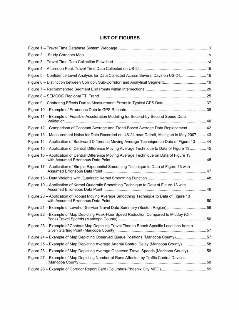
LIST OF FIGURES Figure 1 – Travel Time Database System Webpage....................................................................................iii Figure 2 – Study Corridors Map................................................................................................................... v Figure 3 – Travel Time Data Collection Flowchart........................................................................................vi Figure 4 – Afternoon Peak Travel Time Data Collected on US-24............................................................. 15 Figure 5 – Confidence Level Analysis for Data Collected Across Several Days on US-24........................ 16 Figure 6 – Distinction between Corridor, Sub-Corridor, and Analytical Segment....................................... 19 Figure 7 – Recommended Segment End Points within Intersections......................................................... 20 Figure 8 – SEMCOG Regional TTI Trend................................................................................................... 25 Figure 9 – Chattering Effects Due to Measurement Errors in Typical GPS Data ....................................... 37 Figure 10 – Example of Erroneous Data in GPS Records.......................................................................... 38 Figure 11 – Example of Feasible Acceleration Modeling for Second-by-Second Speed Data
Validation................................................................................................................................... 40 Figure 12 – Comparison of Constant Average and Trend-Based Average Data Replacement ................. 42 Figure 13 – Measurement Noise for Data Recorded on US-24 near Detroit, Michigan in May 2007......... 43 Figure 14 – Application of Backward Difference Moving Average Technique on Data of Figure 13.......... 44 Figure 15 – Application of Central Difference Moving Average Technique to Data of Figure 13 ............... 45 Figure 16 – Application of Central Difference Moving Average Technique on Data of Figure 13
with Assumed Erroneous Data Point ........................................................................................ 45 Figure 17 – Application of Simple Exponential Smoothing Technique to Data of Figure 13 with
Assumed Erroneous Data Point................................................................................................ 47 Figure 18 – Data Weights with Quadratic Kernel Smoothing Function ...................................................... 48 Figure 19 – Application of Kernel Quadratic Smoothing Technique to Data of Figure 13 with
Assumed Erroneous Data Point................................................................................................ 49 Figure 20 – Application of Robust Moving Average Smoothing Technique to Data of Figure 13
with Assumed Erroneous Data Point ........................................................................................ 50 Figure 21 – Example of Level-of-Service Travel Data Summary (Boston Region) .................................... 56 Figure 22 – Example of Map Depicting Peak-Hour Speed Reduction Compared to Midday (Off-
Peak) Travel Speeds (Maricopa County).................................................................................. 56 Figure 23 – Example of Contour Map Depicting Travel Time to Reach Specific Locations from a
Given Starting Point (Maricopa County) ................................................................................... 57 Figure 24 – Example of Map Depicting Observed Queue Positions (Maricopa County)............................ 57 Figure 25 – Example of Map Depicting Average Arterial Control Delay (Maricopa County) ...................... 58 Figure 26 – Example of Map Depicting Average Observed Travel Speeds (Maricopa County) ................ 58 Figure 27 – Example of Map Depicting Number of Runs Affected by Traffic Control Devices
(Maricopa County)..................................................................................................................... 59 Figure 28 – Example of Corridor Report Card (Columbus-Phoenix City MPO).......................................... 59
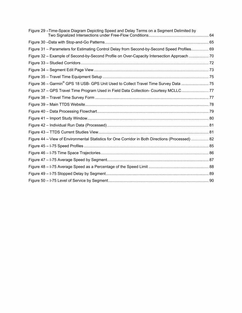
Figure 29 –Time-Space Diagram Depicting Speed and Delay Terms on a Segment Delimited by Two Signalized Intersections under Free-Flow Conditions....................................................... 64
Figure 30 –Data with Stop-and-Go Patterns............................................................................................... 65 Figure 31 – Parameters for Estimating Control Delay from Second-by-Second Speed Profiles................ 69 Figure 32 – Example of Second-by-Second Profile on Over-Capacity Intersection Approach .................. 70 Figure 33 – Studied Corridors..................................................................................................................... 72 Figure 34 – Segment Edit Page View......................................................................................................... 73 Figure 35 – Travel Time Equipment Setup ................................................................................................. 75 Figure 36 – Garmin® GPS 18 USB- GPS Unit Used to Collect Travel Time Survey Data ......................... 75 Figure 37 – GPS Travel Time Program Used in Field Data Collection- Courtesy MCLLC......................... 77 Figure 38 – Travel Time Survey Form ........................................................................................................ 77 Figure 39 – Main TTDS Website................................................................................................................. 78 Figure 40 – Data Processing Flowchart...................................................................................................... 79 Figure 41 – Import Study Window............................................................................................................... 80 Figure 42 – Individual Run Data (Processed) ............................................................................................. 81 Figure 43 – TTDS Current Studies View..................................................................................................... 81 Figure 44 – View of Environmental Statistics for One Corridor in Both Directions (Processed) ................ 82 Figure 45 – I-75 Speed Profiles .................................................................................................................. 85 Figure 46 – I-75 Time Space Trajectories................................................................................................... 86 Figure 47 – I-75 Average Speed by Segment............................................................................................. 87 Figure 48 – I-75 Average Speed as a Percentage of the Speed Limit ....................................................... 88 Figure 49 – I-75 Stopped Delay by Segment.............................................................................................. 89 Figure 50 – I-75 Level of Service by Segment............................................................................................ 90

(This page is intentionally left blank)
SEMCOG Travel Time Data Collection – Page i
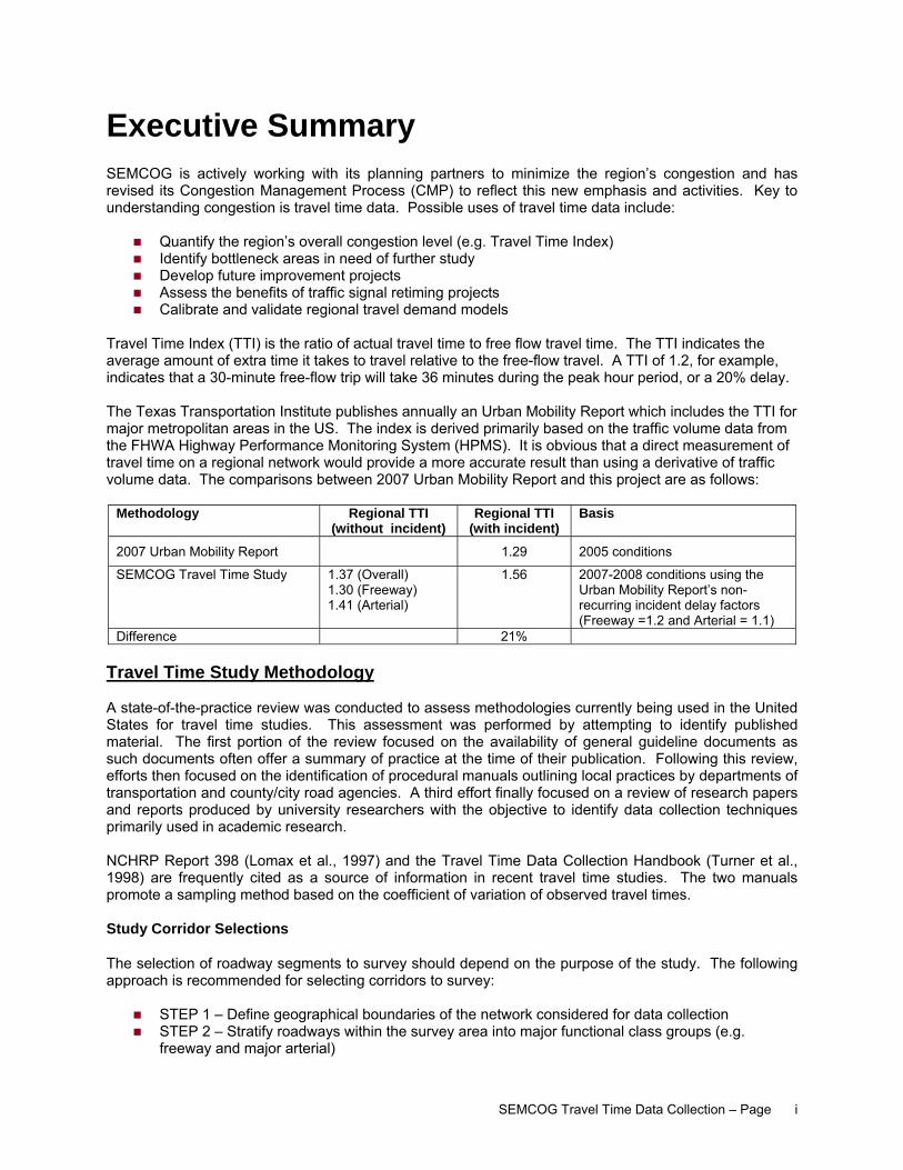
Executive Summary SEMCOG is actively working with its planning partners to minimize the region’s congestion and has revised its Congestion Management Process (CMP) to reflect this new emphasis and activities. Key to understanding congestion is travel time data. Possible uses of travel time data include:
Quantify the region’s overall congestion level (e.g. Travel Time Index) Identify bottleneck areas in need of further study Develop future improvement projects Assess the benefits of traffic signal retiming projects Calibrate and validate regional travel demand models
Travel Time Index (TTI) is the ratio of actual travel time to free flow travel time. The TTI indicates the average amount of extra time it takes to travel relative to the free-flow travel. A TTI of 1.2, for example, indicates that a 30-minute free-flow trip will take 36 minutes during the peak hour period, or a 20% delay. The Texas Transportation Institute publishes annually an Urban Mobility Report which includes the TTI for major metropolitan areas in the US. The index is derived primarily based on the traffic volume data from the FHWA Highway Performance Monitoring System (HPMS). It is obvious that a direct measurement of travel time on a regional network would provide a more accurate result than using a derivative of traffic volume data. The comparisons between 2007 Urban Mobility Report and this project are as follows:
Methodology Regional TTI (without incident)
Regional TTI (with incident)
Basis
2007 Urban Mobility Report 1.29 2005 conditions
SEMCOG Travel Time Study 1.37 (Overall) 1.30 (Freeway) 1.41 (Arterial)
1.56 2007-2008 conditions using the Urban Mobility Report’s non-recurring incident delay factors (Freeway =1.2 and Arterial = 1.1)
Difference 21% Travel Time Study Methodology A state-of-the-practice review was conducted to assess methodologies currently being used in the United States for travel time studies. This assessment was performed by attempting to identify published material. The first portion of the review focused on the availability of general guideline documents as such documents often offer a summary of practice at the time of their publication. Following this review, efforts then focused on the identification of procedural manuals outlining local practices by departments of transportation and county/city road agencies. A third effort finally focused on a review of research papers and reports produced by university researchers with the objective to identify data collection techniques primarily used in academic research. NCHRP Report 398 (Lomax et al., 1997) and the Travel Time Data Collection Handbook (Turner et al., 1998) are frequently cited as a source of information in recent travel time studies. The two manuals promote a sampling method based on the coefficient of variation of observed travel times. Study Corridor Selections
The selection of roadway segments to survey should depend on the purpose of the study. The following approach is recommended for selecting corridors to survey:
STEP 1 – Define geographical boundaries of the network considered for data collection STEP 2 – Stratify roadways within the survey area into major functional class groups (e.g.
freeway and major arterial)
SEMCOG Travel Time Data Collection – Page ii
STEP 3 – Define corridors within each group STEP 4 – Divide the corridors into segments based on the roadway characteristics such as
functional class, speed limits. Connected segments should be group into cluster segments (sub-corridors) that are between 5 to 20 miles in length to make travel time runs cost effective and practical
STEP 5 – Determine number of cluster segments to survey for each group based on sample size required
STEP 6 – Select cluster segments to survey within each functional group using a random sample method
Data Collection Methods Two most common in-vehicle monitoring devices in use today include GPS receivers and electronic Distance Measuring Instruments (DMIs). For the reasons of cost effectiveness and ease of use, it is recommended to use vehicles having GPS measurement capabilities. Test vehicle techniques collect data from vehicles driven along the roadway segments of interest. To be consistent with current practice, it is recommended that travel time runs for planning purposes be conducted using the Average Car Method. Average Car Method is a less restrictive method than others in that a driver does not attempt to pass as many vehicles as the number passing it. The test driver selects instead its travel speed according to its best judgment so as to best match perceived general traffic conditions. In addition, the driver must not exceed posted speed limits along the study corridor. Data Collection Time Periods
A number of issues must be considered when determining periods during which travel time data to be collected. These include:
Periods of congestion Periods of free-flow traffic Invalidating factors (e.g. holidays and weekends)
While travel time data can be collected for any period of the day, depending on the intended use of the data, the periods of greatest interest are usually those during which congestion occurs. For this particular study, the hours of 7:00 to 9:00 AM, 9:30 AM to 11:30 AM, and 4:00 to 6:00 PM were chosen to best represent the AM peak commuter hours, free-flow hours, and PM peak commuter hours, respectively. Phase 1 was conducted using the midday hours of 11:00 AM to 1:00 PM. In order to collect data that was more representative of free flow traffic the midday study period was changed to 9:30 AM to 11:30 AM for Phases 2 & 3. Travel time data collection should be distributed over several days or weeks to ensure that the collected data truly represent average traffic conditions. Because of the possibility of large inconsistencies in data points, this project collected data on Tuesday, Wednesday, and Thursday.
Number of Runs Required
Factors influence the minimum number of runs required to achieve certain accuracy level include:
Average facility-specific coefficients of variation when field data is unavailable Level of confidence in estimated average travel times Allowable error in estimating the average travel times Data collection needs across different days
It is recommended that use of national average coefficients of variation to characterize travel times on roadway segments to survey be considered as preliminary estimates of a minimum number of travel time runs to execute. As soon as field data is available, this information should replace any average value previously assumed.
SEMCOG Travel Time Data Collection – Page iii
Initial requirements for this project are to conduct a minimum of 4 runs per day during peak periods throughout the day over three different weekdays, for a total of at least 12 runs. As confirmed by this project, this is likely to be sufficient for a majority of segments to achieve desired accuracy in estimating weekly average travel times. A statistical method presented in this report should be followed to determine the minimum number of runs. Data Validation, Reporting, and Management
Regardless of the type of GPS used, erroneous measurements can occur as a result of signal loss between the GPS receiver and the satellites or other technical glitches. Potential methods for validating second-by-second travel data include:
Visual inspection Relative inconsistency in speed/position changes Validation of accelerations/deceleration rates
Various methods can be used to correct data, i.e., replace individual erroneous data without touching surrounding valid data. These methods have the advantage of performing minimum alterations to the collected raw data. In most cases, their application will be linked with a search algorithm applying one or more of the validation criteria presented in the report to identify the data points that need to be corrected.
Travel time data collection is often executed with the main intent to quantify congestion. This typically translates into a need to assess average travel speeds and delays incurred by motorists while traveling on surveyed roadway segments. Based on current reporting practice, it is recommended that at a minimum the following information be compiled and reported:
Table providing average observed travel time, travel time variability, average delay and average number of stops for all major travel corridors
Network graph illustrating average observed travel speeds on a segment-by-segment basis Network graph illustrating average observed segment delays on a segment-by-segment basis Network graph illustrating assessed levels of service on a segment-by-segment basis
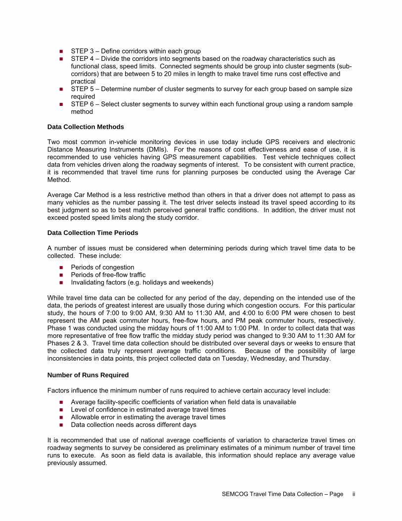
Data management is as important as data collection, validation, and reporting. To ensure that the collected information will have a life that extends beyond the end of the travel time studies, care should be exercised to properly store data. In this project, a web-based Travel Time Database System (TTDS) was deployed to manage all the information generated from the regional travel time study, ranging from raw data upload, validation, statistics, and GIS map integration (Figure 1). The system is live at:
http://www.ms2soft.com/tcds/?loc=semcog_cutline (go to TTDS)
Figure 1 – Travel Time Database System Webpage
SEMCOG Travel Time Data Collection – Page iv
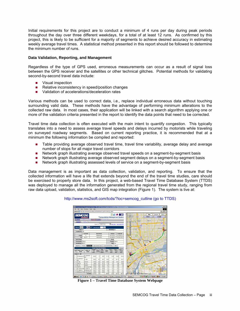
Study Results The 32 corridors (371.5 centerline miles) studied in this project were selected based on their regional significance. These corridors are consistently congested and were given priority because of their importance within the SEMCOG road network. Table 1 below lists all corridors selected for this study grouped by phase completion date.
Table 1 – Study Corridor List Corridor Name From To Length (miles) Date Completed
Phase 1 I-75A 12 Mile Rd Adams Rd 10.9 May 2007 I-94 Rotunda Dr 8 Mile Rd 16.5 April 2007 US-24A 10 Mile Rd Square Lake Rd 9.3 May 2007 M-5 Halsted Rd Bagley St 20.9 May 2007 M-17 I-94 Cross St 9.0 April 2007 M-53 I-94 18 Mile Rd 14.5 May 2007 M-59 I-75 Groesbeck Rd 19.0 May 2007 M-153 Canton Center Rd Evergreen Rd 13.0 May 2007 Phase 1 Total: 113.1
Phase 2 M-1A Jefferson Rd 8 Mile Rd 9.2 September 2007 M-1B 8 Mile Rd Quarton Rd 9.4 October 2007 M-3A Brush St 10 Mile Rd 11.1 September 2007 M-3B 10 Mile Rd 23 Mile Rd 18.8 September 2007 US-12C M-39 Woodward Ave 8.9 September 2007 M-85A Gibralter Rd Schaefer Hwy 13.7 September 2007 M-97A Glenfield St 13 Mile Rd 8.8 September 2007 M-102A Haggerty Rd M-39 11.1 September 2007 M-102B M-39 Mound Rd 9.0 October 2007 US-24C Huron River Dr Ecorse Rd 11.6 October 2007 US-23 Plymouth Rd Grand River Ave 17.9 October 2007 Phase 2 Total: 129.5
Phase 3 US-12B I-275 M-39 11.9 April 2008 MetroA Lahser Rd John R Rd 7.9 April 2008 MetroB John R Rd M-3 11.1 April 2008 MoundA Davison Ave 14 Mile Rd 7.9 April 2008 MoundB 14 Mile Rd M-59 6.2 April 2008 M-10 Fort St 14 Mile Rd 22.2 April 2008 Orchard Lake Rd 8 Mile Rd 14 Mile Rd 6.2 April 2008 I-94B Ann Arbor-Saline Rd Harris St 9.8 April 2008 Whittaker Rd Willis St I-94 5.4 April 2008 I-75D I-94 12 Mile Rd 12.2 April 2008 M-5B Whitmore Lake Rd Prospect St 13.3 April 2008 M-97B 13 Mile Rd M-59 8.3 April 2008 M-102C Mound Rd I-94 6.5 April 2008 Phase 3 Total: 128.9
SEMCOG Travel Time Data Collection – Page v
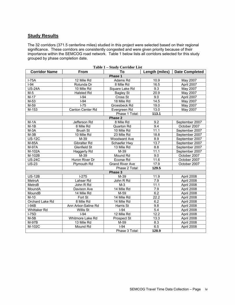
Figure 2 – Study Corridors Map
SEMCOG Travel Time Data Collection – Page vi
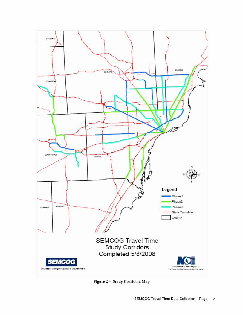
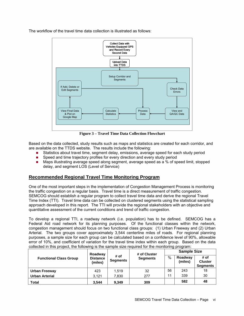
The workflow of the travel time data collection is illustrated as follows:
Setup Corridor and Segments
Collect Data with Vehicles Equipped GPS
and Record Every Second Data
View and QA/QC Data
Upload Data into TTDS
Check Data Errors
Process Data
Calculate Statistics
View Final Data & Plot on
Google Map
If Add, Delete or Edit Segments
Setup Corridor and Segments
Collect Data with Vehicles Equipped GPS
and Record Every Second Data
View and QA/QC Data
Upload Data into TTDS
Check Data Errors
Process Data
Calculate Statistics
View Final Data & Plot on
Google Map
If Add, Delete or Edit Segments
Figure 3 – Travel Time Data Collection Flowchart
Based on the data collected, study results such as maps and statistics are created for each corridor, and are available on the TTDS website. The results include the following:
Statistics about travel time, segment delay, emissions, average speed for each study period Speed and time trajectory profiles for every direction and every study period Maps illustrating average speed along segment, average speed as a % of speed limit, stopped
delay, and segment LOS (Level of Service) Recommended Regional Travel Time Monitoring Program One of the most important steps in the implementation of Congestion Management Process is monitoring the traffic congestion on a regular basis. Travel time is a direct measurement of traffic congestion. SEMCOG should establish a regular program to collect travel time data and derive the regional Travel Time Index (TTI). Travel time data can be collected on clustered segments using the statistical sampling approach developed in this report. The TTI will provide the regional stakeholders with an objective and quantitative assessment of the current conditions and trend of traffic congestion.
To develop a regional TTI, a roadway network (i.e. population) has to be defined. SEMCOG has a Federal Aid road network for its planning purposes. Of the functional classes within the network, congestion management should focus on two functional class groups: (1) Urban Freeway and (2) Urban Arterial. The two groups cover approximately 3,544 centerline miles of roads. For regional planning purposes, a sample size for each group can be calculated based on a confidence level of 90%, allowable error of 10%, and coefficient of variation for the travel time index within each group. Based on the data collected in this project, the following is the sample size required for the monitoring program:
Sample Size Functional Class Group
Roadway Distance (miles)
# of Segments
# of Cluster Segments
% Roadway
(miles) # of
Cluster Segments
Urban Freeway 423 1,519 32 56 243 18 Urban Arterial 3,121 7,830 277 11 339 30
Total 3,544 9,349 309 582 48
SEMCOG Travel Time Data Collection – Page vii
The results of this project indicates that the execution of 4 runs per period per day over 3 days is likely to be sufficient to characterize corridor travel time during the AM peak, off-peak and PM peak periods at a 90% confidence level with a 10% allowable error for both arterial and freeway segments. The effort analysis indicates that average cost of travel time data collection is about $400 per centerline mile. Therefore, SEMCOG should budget for the regional travel time monitoring program about $240,000 for each cycle. Depending on the budget available, the data collection cycle can be 2-3 years. For further information about the project, please contact the following:
Tom Bruff SEMCOG 535 Griswold Street, Suite 300 Detroit, MI 48226 Tel: (313) 324-3340 Fax: (313) 961-4869 Email: [email protected] http://www.semcog.org
Sayeed Mallick SEMCOG 535 Griswold Street, Suite 300 Detroit, MI 48226 Tel: (313) 324-3327 Fax: (313) 961-4869 Email: [email protected] http://www.semcog.org
Ben Chen, PE, PTOE Midwestern Consulting, LLC 3815 Plaza Drive Ann Arbor, MI 48108 Tel: (734) 995-0200 Fax: (734) 995-0599 Email: [email protected] http://www.ms2soft.com
Francois Dion, PhD, P. Eng (formerly Michigan State University) University of Michigan Transportation Research Institute (UMTRI) 2901 Baxter Road Ann Arbor, MI 48109 Tel: (734) 615-6521 Fax: (734) 936-1081 Email: [email protected]

SEMCOG Travel Time Data Collection – Page viii
(This page is intentionally left blank)
SEMCOG Travel Time Data Collection – Page 1
1 Introduction The primary goal of the research outlined in this document was to determine a best approach for collecting travel time data along major travel arterials within the SEMCOG jurisdiction. The objective of this data collection was to obtain information about typical travel conditions experienced by motorists within the metropolitan Detroit area during normal weekdays when travel conditions are not affected by incidents, severe weather or special events. This data is to be used not only to help characterize traffic conditions across the region but also for the development of regional congestion management plans.
A primary issue with any travel time data collection activity is the need to obtain data accurately reflecting reality and considered valid from a statistical standpoint. For this effort, travel time data is to be collected using the average car method with test vehicles equipped with GPS instrumentation allowing collection of second-by-second data. The initial proposal was to use vehicles equipped with accurate distance measuring instruments (DMI) instead of GPS receivers, primarily to eliminate problems associated with the availability of sufficient satellite coverage for accurate GPS measurements in areas with high-rise buildings and to reduce noise measurement errors. However, use of GPS-equipped vehicles was finally preferred as this equipment is less expensive, easy to install in any vehicle, and thus, more likely to be reflective of travel time studies conducted by various transportation agencies.
The following sections of this report document results of several investigations that were conducted to develop a valid data collection plan for the proposed travel time study:
• Review of state-of-practice regarding application of sampling techniques to travel time studies • Data collection methods • Selection of survey corridors • Corridor segmentation • Multi-year data collection approach • Benchmarking needs • Data collection periods • Sample size estimation techniques • Factors affecting sampling requirements • Data validation • Data storage • Estimation of trip characterization parameters
SEMCOG Travel Time Data Collection – Page 2
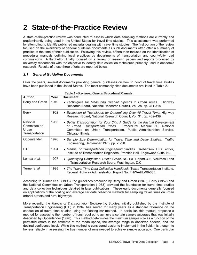
2 State-of-the-Practice Review A state-of-the-practice review was conducted to assess which data sampling methods are currently and predominantly being used in the United States for travel time studies. This assessment was performed by attempting to identify published material dealing with travel time studies. The first portion of the review focused on the availability of general guideline documents as such documents often offer a summary of practice at the time of their publication. Following this review, efforts then focused on the identification of procedural manuals outlining local practices by departments of transportation and county/city road commissions. A third effort finally focused on a review of research papers and reports produced by university researchers with the objective to identify data collection techniques primarily used in academic research. Results of these three efforts are reported below.
2.1 General Guideline Documents
Over the years, several documents providing general guidelines on how to conduct travel time studies have been published in the United States. The most commonly cited documents are listed in Table 2.
Table 2 – Reviewed General Procedural Manuals Author Year Document Berry and Green 1949
• Techniques for Measuring Over-All Speeds in Urban Areas. Highway
Research Board, National Research Council, Vol. 28, pp. 311-318.
Berry 1952 • Evaluation of Techniques for Determining Over-All Travel Time. Highway Research Board, National Research Council, Vol. 31, pp. 432-439.
National Committee on Urban Transportation
1953 • Better Transportation for Your City: A Guide for the Factual Development of Urban Transportation Plans. Procedural Manual 3B, National Committee on Urban Transportation, Public Administration Service, Chicago, Illinois.
Oppenlander 1976 • Sample Size Determination for Travel Time and Delay Studies. Traffic Engineering, September 1976, pp. 25-28.
ITE 1994 • Manual of Transportation Engineering Studies. Robertson, H.D., editor, Institute of Transportation Engineers, Prentice Hall, Englewood Cliffs, NJ.
Lomax et al. 1997 • Quantifying Congestion: User’s Guide. NCHRP Report 398, Volumes I and II. Transportation Research Board, Washington, D.C.
Turner et al. 1998 • The Travel Time Data Collection Handbook. Texas Transportation Institute, Federal Highway Administration Report No. FHWA-PL-98-035.
According to Turner et al. (1998), the guidelines produced by Berry and Green (1949), Berry (1952) and the National Committee on Urban Transportation (1953) provided the foundation for travel time studies and data collection techniques detailed in later publications. These early documents generally focused on applications of the floating and average car data collection methods for sampling travel times on urban arterial streets and rural highways.
More recently, the Manual of Transportation Engineering Studies, initially published by the Institute of Transportation Engineering (ITE) in 1994, has served for many years as a standard reference on the conduction of travel time studies using the floating car method. In particular, this manual proposes a method for assessing the number of runs required to achieve a certain sample accuracy that was initially described by Oppenlander (1976). This method determines the minimum sample size as a function of the permitted errors in the estimate of the mean speed, the average range in observed speeds, and the desired confidence level. While this method is considered easier to implement in the field, it is thought to be less reliable in assessing the true number of runs needed to achieve sample accuracy. One particular
SEMCOG Travel Time Data Collection – Page 3
critique is that this method tends to underestimate the number of runs required (Quiroga and Bullock, 1998a).
More recent assessments of the state of practice are found in NCHRP (National Cooperative Highway Research Program) Report 398 (Lomax et al., 1997) and the Travel Time Data Collection Handbook (Turner et al., 1998). Both documents are frequently cited as a source of information in recent travel time studies. NCHRP Report 398 provides technical guidelines for measuring and estimating travel times, with particular focus on how to determine the number segments to be sampled, estimate the number of required runs, and use surrogate measures for estimating speeds. The Travel Time Data Collection Handbook, which heavily draws upon the conclusion of NCHRP Report 398, provides procedural details for a range of data collection techniques, including the traditional floating car method, license plate matching, and probe vehicles using GPS or DMI instrumentation. A significant difference with respect to the ITE’s Manual of Transportation Engineering Studies in both documents is a shift in the recommended method to assess the number of runs required. Instead of focusing on the range of running speeds method, the two manuals promote instead a sampling method based on the coefficient of variation of observed travel times. This approach, which is thought to be more accurate, also appears to be generally favored among transportation textbooks, as it is described in such textbooks as those written by May (1990) and Garber and Hoel (2002).
2.2 Documents from State Departments of Transportation and Local Agencies
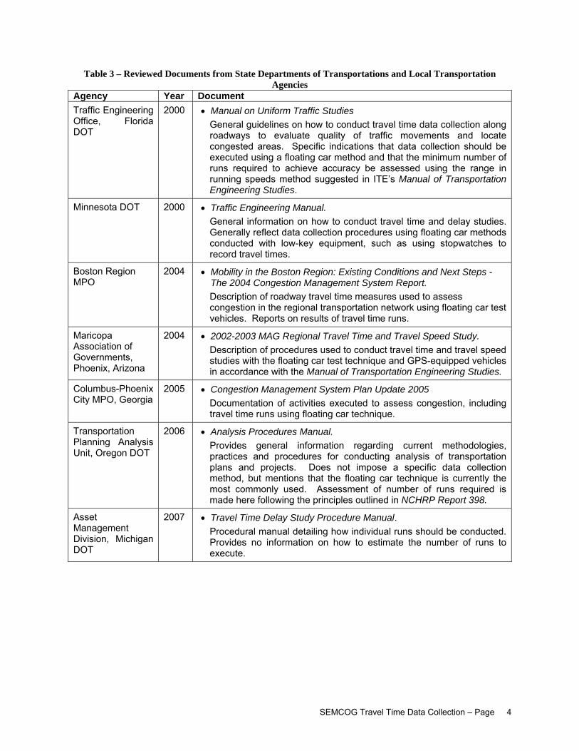
A search for procedural manuals produced by state departments of transportation and county/city road commissions has lead to the identification of a number of documents providing information about travel time studies. These documents are listed and briefly detailed in Table 3.
The documents reviewed only provide general information about how to conduct travel time studies or how specific studies were conducted. No specific step-by-step information is provided as to how to execute travel time studies and analyze collected data. The documents generally seem to indicate that travel time studies are typically executed using floating car test vehicle methods following guidelines from the ITE’s Manual of Transportation Engineering Studies, NCHRP Report 398 or the Travel Time Data Collection Handbook.
Recent travel time studies conducted as part of academic research projects generally appear to follow the sampling guidelines described in NCHRP Report 398 or the Travel Time Data Collection Handbook. Very few recent studies, outside those executed for the Florida DOT, appear to use the range sampling method described in the Manual of Transportation Engineering Studies published by ITE or the Manual on Uniform Traffic Studies published by the Florida DOT.
SEMCOG Travel Time Data Collection – Page 4
Table 3 – Reviewed Documents from State Departments of Transportations and Local Transportation Agencies
Agency Year Document Traffic Engineering Office, Florida DOT
2000
• Manual on Uniform Traffic Studies General guidelines on how to conduct travel time data collection along roadways to evaluate quality of traffic movements and locate congested areas. Specific indications that data collection should be executed using a floating car method and that the minimum number of runs required to achieve accuracy be assessed using the range in running speeds method suggested in ITE’s Manual of Transportation Engineering Studies.
Minnesota DOT 2000 • Traffic Engineering Manual. General information on how to conduct travel time and delay studies. Generally reflect data collection procedures using floating car methods conducted with low-key equipment, such as using stopwatches to record travel times.
Boston Region MPO
2004 • Mobility in the Boston Region: Existing Conditions and Next Steps - The 2004 Congestion Management System Report. Description of roadway travel time measures used to assess congestion in the regional transportation network using floating car test vehicles. Reports on results of travel time runs.
Maricopa Association of Governments, Phoenix, Arizona
2004 • 2002-2003 MAG Regional Travel Time and Travel Speed Study. Description of procedures used to conduct travel time and travel speed studies with the floating car test technique and GPS-equipped vehicles in accordance with the Manual of Transportation Engineering Studies.
Columbus-Phoenix City MPO, Georgia
2005 • Congestion Management System Plan Update 2005 Documentation of activities executed to assess congestion, including travel time runs using floating car technique.
Transportation Planning Analysis Unit, Oregon DOT
2006 • Analysis Procedures Manual. Provides general information regarding current methodologies, practices and procedures for conducting analysis of transportation plans and projects. Does not impose a specific data collection method, but mentions that the floating car technique is currently the most commonly used. Assessment of number of runs required is made here following the principles outlined in NCHRP Report 398.
Asset Management Division, Michigan DOT
2007 • Travel Time Delay Study Procedure Manual. Procedural manual detailing how individual runs should be conducted. Provides no information on how to estimate the number of runs to execute.
SEMCOG Travel Time Data Collection – Page 5
3 Data Collection Methods Techniques currently used for collecting travel time data can be categorized into three broad groups:
• Test vehicle techniques • Probe vehicle techniques • Traffic sampling techniques
3.1 Test Vehicle Techniques
Test vehicle techniques collect travel time data from vehicles intentionally driven along the roadway segments of interest for the purpose of collecting data. In most cases, the test vehicle is equipped with instruments to record travel information. While early travel time studies simply relied on the use of stopwatch or timers to mark the time taken by a vehicle to travel from one reference point to another, recent studies rely more heavily on the use of automated equipment allowing information such as position and speed to be recorded on a second-by-second basis.
The two most common in-vehicle monitoring devices in use today include GPS receivers and electronic Distance Measuring Instruments (DMIs). These systems are briefly summarized below:
• GPS receivers use signals emitted by an array of satellites to locate the position of a vehicle and determine its speed by triangulation. Basic GPS systems have a typical accuracy of 50 ft for position location and 0.1 mph for steady-state measured speed. Location accuracy can be as high as 6 ft when line of sights to at least 12 satellites can be maintained. Measurement errors are due to various factors affecting signal transmission between the satellites and a receiver on the ground. Typical error sources include atmospheric effects, multi-path effects resulting from the signal reflecting off surrounding terrain and buildings, and errors associated with the calculation of correct signal travel time due to ephemeris error and satellite clock error. Greater accuracy can be obtained with the use of Differential GPS (DGPS), which uses base satellite communication stations at known locations to produce correction factors for the GPS measurements.
• Electronic DMIs estimate speeds and traveled distance from a sensor attached to a vehicle’s transmission. Sensors typically monitor pulses sent by the transmission based on the vehicle’s speed and convert these pulses into distance measurements. Reliance on information provided directly by the vehicle results in typical measurements accuracy in the order of 1 foot per traveled mile. A typical error source associated with a DMI is improper calibration of the instrument. To ensure accurate distance measurements, the instrument must be calibrated frequently to account for differing tire pressure, weather, and user operation. If calibration is not performed regularly, the error will compound over time and eventually cause measurements to be irrelevant.
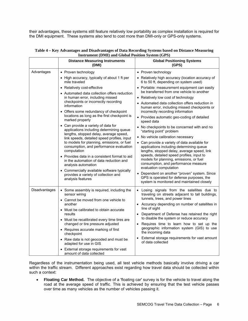
Table 4 summarizes the main advantages and disadvantages associated with the use of GPS and DMI instrumentation for recorded travel data. The main advantage of DMI-based systems is its ability to measure distances with high accuracy. In comparison, the dependence of GPS measurements on timely communications with satellites a hundred miles in the sky create some potential for delayed signals and reduced measurement accuracy. Measurements from GPS systems may also not be possible altogether at locations where lines of sight with at least three satellites cannot be maintained. On the other hand, GPS systems offer the advantage of providing direct location positioning, which then facilitate displaying collected data on GIS maps. With a DMI, the location of the data collection must be recorded separately as these systems only measure relative distance traveled from a start point.
While agencies only had in the past the choice of using either GPS or DMI, many equipment manufacturers are now offering systems combining both technologies. In these systems, distance measurements are primarily obtained through DMI technology while GPS sensing capabilities are used for location positioning, data consistency checks, and interfacing with GIS mapping software. Despite
SEMCOG Travel Time Data Collection – Page 6
their advantages, these systems still feature relatively low portability as complex installation is required for the DMI equipment. These systems also tend to cost more than DMI-only or GPS-only systems.
Table 4 – Key Advantages and Disadvantages of Data Recording Systems based on Distance Measuring
Instrument (DMI) and Global Position System (GPS) Distance Measuring Instruments
(DMI) Global Positioning Systems
(GPS)
Advantages • Proven technology • High accuracy, typically of about 1 ft per
mile traveled • Relatively cost-effective • Automated data collection offers reduction
in human error, including missed checkpoints or incorrectly recording information
• Offers some redundancy of checkpoint locations as long as the first checkpoint is marked properly
• Can provide a variety of data for applications including determining queue lengths, stopped delay, average speed, link speeds, detailed speed profiles, input to models for planning, emissions, or fuel consumption, and performance evaluation computation
• Provides data in a consistent format to aid in the automation of data reduction and analysis automation
• Commercially available software typically provides a variety of collection and analysis features
• Proven technology • Relatively high accuracy (location accuracy of
6 to 50 ft, depending on system used) • Portable: measurement equipment can easily
be transferred from one vehicle to another • Relatively low cost of technology • Automated data collection offers reduction in
human error, including missed checkpoints or incorrectly recording information
• Provides automatic geo-coding of detailed speed data
• No checkpoints to be concerned with and no “starting point” problem
• No vehicle calibration necessary • Can provide a variety of data available for
applications including determining queue lengths, stopped delay, average speed, link speeds, detailed speed profiles, input to models for planning, emissions, or fuel consumption, and performance measure evaluation computation
• Dependent on another “proven” system. Since GPS is operated for defense purposes, the system is monitored and maintained closely
Disadvantages • Some assembly is required, including the sensor wiring
• Cannot be moved from one vehicle to another
• Must be calibrated to obtain accurate results
• Must be recalibrated every time tires are changed or tire pressure adjusted
• Requires accurate marking of first checkpoint
• Raw data is not geocoded and must be adapted for use in GIS
• External storage requirements for vast amount of data collected
• Losing signals from the satellites due to traveling on streets adjacent to tall buildings, tunnels, trees, and power lines
• Accuracy depending on number of satellites in line of sight
• Department of Defense has retained the right to disable the system or reduce accuracy
• Requires time to learn how to set up the geographic information system (GIS) to use the incoming data
• External storage requirements for vast amount of data collected
Regardless of the instrumentation being used, all test vehicle methods basically involve driving a car within the traffic stream. Different approaches exist regarding how travel data should be collected within such a context:
• Floating Car Method. The objective of a 'floating car' survey is for the vehicle to travel along the road at the average speed of traffic. This is achieved by ensuring that the test vehicle passes over time as many vehicles as the number of vehicles passing it.
SEMCOG Travel Time Data Collection – Page 7
• Average Car Method. This is a less restrictive method than the floating car in that a driver does not attempt to pass as many vehicles as the number passing it. The test driver selects instead its travel speed according to its best judgment so as to best match perceived general traffic conditions.
• Maximum Car Method. With this technique the driver travels at the posted speed limit unless impeded by traffic.
• Chase Car Method. This technique sees individual vehicles randomly selected from the traffic stream and followed. This gives a sample of the performance of actual vehicles in the traffic stream rather than the performance of the test driver.
Based on frequency of citation, the floating car approach currently appears to be the most commonly used method for conducting travel time studies as this method is generally thought to produce reliable results. However, according to the Minnesota DOT’s Traffic Engineering Manual, tests have shown that some inaccuracies occur when utilizing this technique during periods of congested flow on multilane highways and on roads with very low traffic volumes. Local experience further suggests that the average-car technique has generally resulted in more representative test speeds.
The Travel Time Data Collection Handbook further indicates that most travel time studies are not strict implementation of the floating car or average car methods but tend instead to be a hybrid of both methods. In particular, according to the handbook, differences between individual test drivers are more likely to account for more variations than exist between the floating car and average car data collection methods themselves, thus allowing for some flexibility in the choice of a specific survey method. For these reasons, use of either the floating car or average car methods can be recommended for conducting travel time studies.
Regardless of the instrumentation or survey method used, the primary advantages associated with the test vehicle technique are:
• Provision of consistent data collection through the determination of driving style (floating car, average car, etc.).
• Use of in-board monitoring technology allowing detailed data covering the entire study corridor to be collected.
• Relatively low initial cost.
On the other hand, primary disadvantages include:
• Requires quality control to account for potential errors from drivers and potential measurement errors from equipment.
• Ability to collect detailed data, such as second-by-second data, can lead to data storage difficulties.
• Travel time estimates are based on only a few samples, particularly when compared to sample sizes that can be obtained with other techniques.
3.2 Probe Vehicle Techniques
Probe vehicle techniques utilize passive instrumented vehicles and remote sensing devices to collect travel information. Equipped vehicles can be personal cars, public transit vehicles or commercial vehicles. The primary difference with the test vehicle techniques is that drivers of probe vehicles are not necessarily instructed to travel a specific roadway segment in a specific manner at a specific time. Travel data is collected as the vehicle is being used for normal purposes by its owner/driver.
The main interest of the transportation community in probe vehicle techniques is associated with the ability to collect travel information on any street on which equipped vehicles are traveling and at any period of the day. Primary applications are not to collect travel time information on specific roadways since there is no means to control when and where probe vehicles are driven. Probe vehicle techniques
SEMCOG Travel Time Data Collection – Page 8
tend to be used to collect information for general transportation system monitoring, incident detection, route guidance applications, etc.
Various technologies have been used in monitoring the movement of probe vehicles. In most cases, event-based data recording equipment linked to sensors installed onboard a vehicle are used to record statistics of interest at specific intervals, such as the location and speed of a vehicle. Communication equipment is then used to periodically, or continuously, allow data downloads to a central data management facility.
3.3 Traffic Sampling Techniques
Instead of relying on information provided by specifically instrumented vehicles, traffic sampling techniques collect travel time information by remotely monitoring the time taken by individual vehicles to travel across a roadway segment. These techniques are similar to having someone standing next to a road and tracking the movement of individual vehicles.
Over the years, various techniques have been proposed to automatically monitor and collect travel times on specific roadway segments. These techniques essentially attempt to match records of vehicle passage at a given location with records of subsequent passage of the same vehicle at some downstream location. The most commonly cited sampling techniques currently include:
• License Plate Matching. License plate matching relies on video signal processing algorithms to extract the license number of vehicles passing at each detection point. Travel time between two locations is then obtained by simply calculating the time difference between detection records for the same vehicle at the two locations.
• Automatic Vehicle Identification (AVI). Similar to license plate matching, AVI systems estimate travel times between two locations by matching detection records of specific vehicles at each location. In this case, a vehicle is typically uniquely identified through the electronic signature of a transponder installed onboard the vehicle. These transponders are generally the same as those currently used for electronic toll collection.
• Cellular Geolocation Tracking. Cellular geolocation is an emerging technique that is still currently under testing and which attempts to take advantage of the fact that all cell phones are now required being equipped with a GPS locator to determine their position at all times. By tracking the location of active cell phones on a second-by-second basis, it is then possible to determine whether the cell phone is likely to be in a vehicle, and if so, the position and speed of the vehicle in which the phone is located. If a large enough sample is obtained, estimates of average travel times on the roadway segment being monitored could then be developed.
• Vehicle Signature Matching. This is another emerging technique that is still under research. This technique calculates travel time by matching unique vehicle signatures between sequential observation points. It differs from AVI identification methods in that it requires no specific instrumentation to be installed onboard the probe vehicles. Matches are made only from information provided by traditional traffic sensors, such a loop detectors or video cameras.
All of the above sampling techniques allow travel time data to be collected from much larger samples than traditional test vehicle techniques. Instead of collecting only 4 to 12 travel time samples, it may be possible to collect travel time data for 10 or 30% of all vehicles passing a given point. Some techniques, such as license plate matching even theoretically allow 100% of passing vehicles to be sampled, if no errors occur when extracting license plate information.
However, various constraints still prevent their widespread use. For instance, the requirement that a fair proportion of vehicles be equipped with transponders usually prevents the utilization of AVI-based sampling techniques outside tolled freeways. While use of AVI transponders for collecting freeway travel times has been very successful in Houston, Texas, a similar effort in San Antonio has not been successful (Carter et al., 2000). The difference between the two cities is that Houston residents use AVI transponders for traveling on the city’s toll freeways while such freeways exist around San Antonio. Thus,
SEMCOG Travel Time Data Collection – Page 9
while AVI transponders were made available for distribution, San Antonio drivers were very reluctant to install monitoring equipment in their vehicles without a clear perceived benefit. As a result, sample rates of less than 1% were obtained in San Antonio for the various roadway segments monitored, while sample rates exceeding 20 and 30% were often obtained for Houston’s monitored freeway sections.
While license plate matching equipment can theoretically be installed at any desired location, special setup may be required to obtain the desired vantage point, significantly reducing system portability. Some states may also require special permits to utilize this equipment to ensure that the system is not being used for tracking motorists other than to collect generic travel information. Finally, both cellular geolocation tracking and vehicle signature matching are still mainly in the development stage and have not yet been deployed other than for system testing/evaluation.
3.4 Recommended Techniques
To be consistent with current practice, it is recommended that travel time runs for general planning purposes be conducted using the floating-car or average test vehicle technique. While the floating car technique currently appears to be by far the most frequently used, some agencies have found that the average test vehicle technique may produce travel time estimates that are better reflective of reality and recommend its use instead of the floating car technique.
Travel time runs can further be executed using test vehicles equipped with either GPS or DMI sensors. In this case, it is strongly recommended to use vehicles having GPS measurement capabilities. GPS equipment is not only easier to implement but also facilitates interactions with GIS software by allowing direct measurement of a vehicle’s position in a transportation network. Preferably, systems combining GPS and DMI equipment can be used, if available.
Use of probe vehicles and traffic sampling techniques may also be considered where the required sensing equipment is available or already in place.
SEMCOG Travel Time Data Collection – Page 10
4 Selection of Data Collection Periods A number of issues must be considered when determining periods during which travel time data must and can be collected. These include:
• Periods for congestion characterization • Periods for free-flow travel time characterization • Invalidating factors
4.1 Periods for Congestion Characterization
While travel time data can be collected for any period of the day, depending on the intended use of the data, the periods of greatest interest are usually those during which congestion exist. These periods typically correspond to the morning and evening weekday commutes, which typically extend from 6:00 AM to 9:00 AM and from 4:00 PM to 7:00 PM in most large cities. Travel times during midday periods may also be of interest if significant traffic exists during these periods.
Another general recommendation is that travel time data collection should be distributed over several days or weeks to ensure that the collected data truly represent average traffic conditions. While it is possible to ensure that data collection on a specific segment is not affected by inclement weather or incidents, secondary effects from incidents on other roads, often miles away, may be difficult to assess. Limiting the data collection to a single day creates a potential for collected travel time data that may be skewed by events occurring on other roads, such as a major incident on a nearby freeway causing traffic diversions. By spreading the data collection over several days, there are fewer risks that a single event may indirectly affect the data collection and invalidate the whole effort.
4.2 Periods for Free-flow Travel Time Characterization
At the other end, an interest may also exist in collecting travel time data during periods of low traffic for the purpose of estimating free-flow travel time and obtaining a reference situation against which congestion levels can be assessed. For many arterials, the best weekday periods to collect free-flow travel times would be during the middle of the day, typically between 10:00 to 11:00 AM and 1:00 to 3:00 PM, or late in the evening, typically after 7:00 PM. Data collection between 11:00 AM and 1:00 PM is also sometimes suggested. However, use of this period for collecting free-flow travel time should only be considered if there is no significant surge in lunch traffic creating a situation in which drivers may be somewhat constrained by other traffic.
4.3 Invalidating Factors
Most manuals on travel time studies recommend that travel time data should only be collected under good weather conditions and in the absence of construction, incidents and unusual traffic/pedestrian patterns on the roadway that may affect driver behavior to ensure that the collected data is truly reflective of normal travel conditions on the roadway of interest.
SEMCOG Travel Time Data Collection – Page 11
5 Factors Affecting Sampling Activities A number of factors influence sampling activities and determination of a minimum number of travel time runs to be executed to achieve certain accuracy:
• Use of average facility-specific coefficients of variation when field data is unavailable • Level of confidence in estimated average travel times • Allowable error in estimating the average travel time • Data collection needs across different days
5.1 Coefficients of Variation of Travel Times
The coefficient of variation of travel times has a significant impact on the determination of the number of runs necessary to achieve certain accuracy. From a theoretical standpoint, the coefficient of variation to use in this determination should be the true coefficients for travel times along a segment or corridor. However, this coefficient is usually not known ahead of time. Often, initial estimates of the number of runs to execute are based on the use of coefficients of variation from previous analyses of generic coefficients listed in reference documents and characterizing typical traffic conditions across a range of similar corridors or segments. After a few runs have been executed, the initially assumed coefficient of variation can be replaced by the estimated coefficient to allow a more precise estimate of the minimum number of required runs to be calculated based on the site-specific traffic conditions. The true coefficient of variation is likely never known as obtaining this coefficient would require a very large sample of travel times.
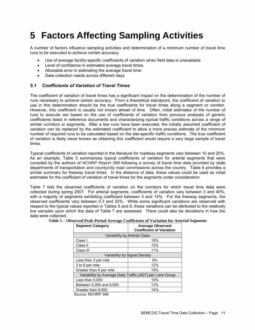
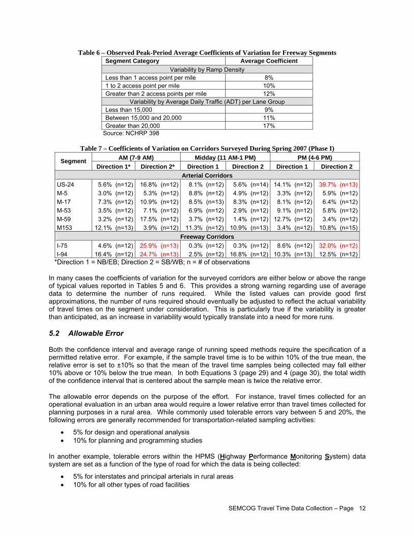
Typical coefficients of variation reported in the literature for roadway segments vary between 10 and 20%. As an example, Table 5 summarizes typical coefficients of variation for arterial segments that were compiled by the authors of NCHRP Report 398 following a survey of travel time data provided by state departments of transportation and county/city road commissions across the country. Table 6 provides a similar summary for freeway travel times. In the absence of data, these values could be used as initial estimates for the coefficient of variation of travel times for the segments under consideration.
Table 7 lists the observed coefficients of variation on the corridors for which travel time data were collected during spring 2007. For arterial segments, coefficients of variation vary between 3 and 40%, with a majority of segments exhibiting coefficient between 3 and 14%. For the freeway segments, the observed coefficients vary between 0.3 and 32%. While some significant variations are observed with respect to the typical values reported in Tables 5 and 6, these variations can be attributed to the relatively low samples upon which the data of Table 7 are assessed. There could also be deviations in how the data were collected.
Table 5 – Observed Peak-Period Average Coefficients of Variation for Arterial Segments Segment Category Average Observed
Coefficient of Variation Variability by Arterial Class
Class I 19% Class II 15% Class III 11%
Variability by Signal Density Less than 3 per mile 9% 3 to 6 per mile 12% Greater than 6 per mile 15%
Variability by Average Daily Traffic (ADT) per Lane Group Less than 5,000 10% Between 5,000 and 9,000 13% Greater than 9,000 14%
Source: NCHRP 398
SEMCOG Travel Time Data Collection – Page 12
Table 6 – Observed Peak-Period Average Coefficients of Variation for Freeway Segments Segment Category Average Coefficient
Variability by Ramp Density Less than 1 access point per mile 8% 1 to 2 access point per mile 10% Greater than 2 access points per mile 12%
Variability by Average Daily Traffic (ADT) per Lane Group Less than 15,000 9% Between 15,000 and 20,000 11% Greater than 20,000 17%
Source: NCHRP 398
Table 7 – Coefficients of Variation on Corridors Surveyed During Spring 2007 (Phase I) AM (7-9 AM) Midday (11 AM-1 PM) PM (4-6 PM) Segment
Direction 1* Direction 2* Direction 1 Direction 2 Direction 1 Direction 2 Arterial Corridors
US-24 5.6% (n=12) 16.8% (n=12) 8.1% (n=12) 5.6% (n=14) 14.1% (n=12) 39.7% (n=13)M-5 3.0% (n=12) 5.3% (n=12) 8.8% (n=12) 4.9% (n=12) 3.3% (n=12) 5.9% (n=12)M-17 7.3% (n=12) 10.9% (n=12) 8.5% (n=13) 8.3% (n=12) 8.1% (n=12) 6.4% (n=12)M-53 3.5% (n=12) 7.1% (n=12) 6.9% (n=12) 2.9% (n=12) 9.1% (n=12) 5.8% (n=12)M-59 3.2% (n=12) 17.5% (n=12) 3.7% (n=12) 1.4% (n=12) 12.7% (n=12) 3.4% (n=12)M153 12.1% (n=13) 3.9% (n=12) 11.3% (n=12) 10.9% (n=13) 3.4% (n=12) 10.8% (n=15)
Freeway Corridors I-75 4.6% (n=12) 25.9% (n=13) 0.3% (n=12) 0.3% (n=12) 8.6% (n=12) 32.0% (n=12)I-94 16.4% (n=12) 24.7% (n=13) 2.5% (n=12) 16.8% (n=12) 10.3% (n=13) 12.5% (n=12)
*Direction 1 = NB/EB; Direction 2 = SB/WB; n = # of observations
In many cases the coefficients of variation for the surveyed corridors are either below or above the range of typical values reported in Tables 5 and 6. This provides a strong warning regarding use of average data to determine the number of runs required. While the listed values can provide good first approximations, the number of runs required should eventually be adjusted to reflect the actual variability of travel times on the segment under consideration. This is particularly true if the variability is greater than anticipated, as an increase in variability would typically translate into a need for more runs.
5.2 Allowable Error
Both the confidence interval and average range of running speed methods require the specification of a permitted relative error. For example, if the sample travel time is to be within 10% of the true mean, the relative error is set to ±10% so that the mean of the travel time samples being collected may fall either 10% above or 10% below the true mean. In both Equations 3 (page 29) and 4 (page 30), the total width of the confidence interval that is centered about the sample mean is twice the relative error.
The allowable error depends on the purpose of the effort. For instance, travel times collected for an operational evaluation in an urban area would require a lower relative error than travel times collected for planning purposes in a rural area. While commonly used tolerable errors vary between 5 and 20%, the following errors are generally recommended for transportation-related sampling activities:
• 5% for design and operational analysis • 10% for planning and programming studies
In another example, tolerable errors within the HPMS (Highway Performance Monitoring System) data system are set as a function of the type of road for which the data is being collected:
• 5% for interstates and principal arterials in rural areas • 10% for all other types of road facilities
SEMCOG Travel Time Data Collection – Page 13
The ITE Manual of Transportation Engineering Studies recommend on its end permissible errors expressed as range in allowable speed rather than a percentage error. Recommended permissible errors for specific activities are as follows:
• Before and after studies: ±1 to ±3 mph (±3 recommendation in Florida for studies involving efficiency, and ±2 for studies involving safety)
• Traffic operations, trend analysis, economic evaluation: ±2 to ±4 mph • Transportation planning and highway needs studies: ±3 to ±5 mph
In a similar approach, the Georgia Department of Transportation recommends use of the following errors for reporting freeway segment travel times on variable message signs:
• ±1 min for short trips (5-6 min) • ±2 min for most conditions • ±3 min for long trips (25-28 min)
In general, a lower tolerable error will tend to increase the number of travel time runs to be executed to attain a certain confidence level. For cases in which a specific value is not set by institutional guidelines, use of a 10% tolerable error is recommended as use of this value appears to be fairly common.
5.3 Confidence Level
Typical confidence intervals for travel time studies vary between 80 and 95%, with a majority of studies reporting using a confidence level of 90 or 95%. The theoretical recommendation is always to use the highest confidence level possible to provide more accurate results. However, since such an approach tends to yield significantly high numbers of required runs, it is not always practical to require the use of a 95 or even 99% confidence level. For this reason, compromises reflecting the intended use of the data are generally made.
Suggested confidence levels in NCHRP Report 398 for the collection of travel data are:
• Between 80 and 90% for planning activities • Between 90 and 95% for operational analyses
Confidence levels used in HPMS to determine the number of required segments to sample are based on the type of facility being surveyed. The following are minimum confidence level requirements defined by FHWA for the collection of data pertaining to specific types of roadway segments in different categories of areas:
• Rural areas: o 80% for major collectors o 90% for minor arterials, principal arterials, and interstates
• Small urban areas: o 80% for collectors o 90% for minor arterials, principal arterials, expressways and interstates
• Urbanized areas with less than 200,000 population that are not in a NAAQS Non-attainment or maintenance area:
o 80% for collectors, principal arterials expressways and interstates o 90% for minor arterials
• Urbanized areas with less than 200,000 population that are in a NAAQS (National Ambient Air Quality Standards) Non-attainment or maintenance area:
o 80% for collectors o 90% for minor arterials, principal arterials expressways and interstates
• Donut areas: o 90% for minor arterials and collectors
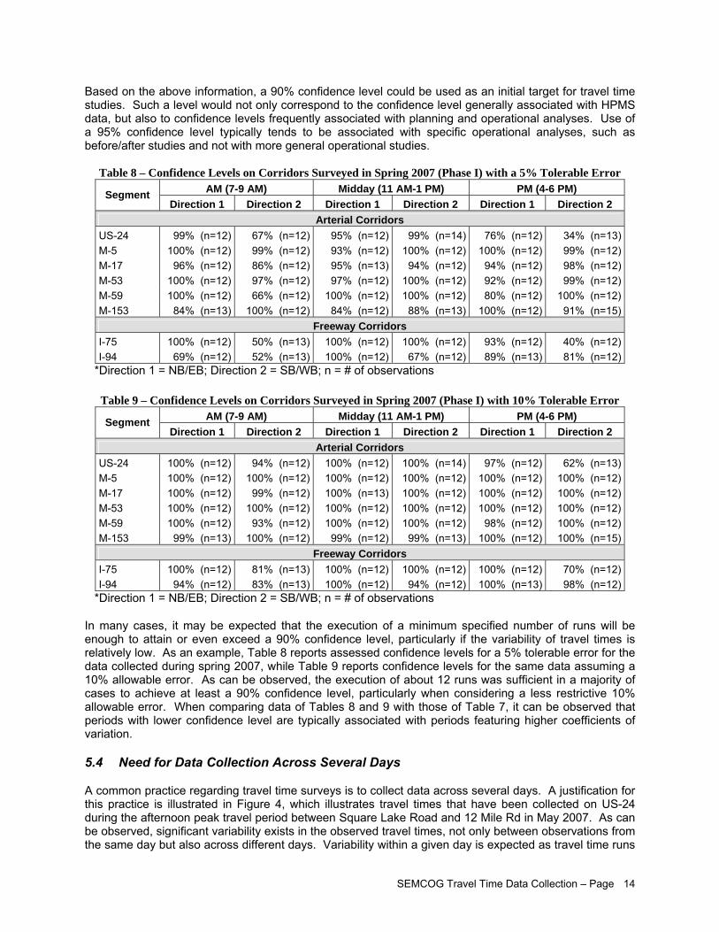
SEMCOG Travel Time Data Collection – Page 14
Based on the above information, a 90% confidence level could be used as an initial target for travel time studies. Such a level would not only correspond to the confidence level generally associated with HPMS data, but also to confidence levels frequently associated with planning and operational analyses. Use of a 95% confidence level typically tends to be associated with specific operational analyses, such as before/after studies and not with more general operational studies.
Table 8 – Confidence Levels on Corridors Surveyed in Spring 2007 (Phase I) with a 5% Tolerable Error AM (7-9 AM) Midday (11 AM-1 PM) PM (4-6 PM) Segment
Direction 1 Direction 2 Direction 1 Direction 2 Direction 1 Direction 2 Arterial Corridors
US-24 99% (n=12) 67% (n=12) 95% (n=12) 99% (n=14) 76% (n=12) 34% (n=13)M-5 100% (n=12) 99% (n=12) 93% (n=12) 100% (n=12) 100% (n=12) 99% (n=12)M-17 96% (n=12) 86% (n=12) 95% (n=13) 94% (n=12) 94% (n=12) 98% (n=12)M-53 100% (n=12) 97% (n=12) 97% (n=12) 100% (n=12) 92% (n=12) 99% (n=12)M-59 100% (n=12) 66% (n=12) 100% (n=12) 100% (n=12) 80% (n=12) 100% (n=12)M-153 84% (n=13) 100% (n=12) 84% (n=12) 88% (n=13) 100% (n=12) 91% (n=15)
Freeway Corridors I-75 100% (n=12) 50% (n=13) 100% (n=12) 100% (n=12) 93% (n=12) 40% (n=12)I-94 69% (n=12) 52% (n=13) 100% (n=12) 67% (n=12) 89% (n=13) 81% (n=12)
*Direction 1 = NB/EB; Direction 2 = SB/WB; n = # of observations
Table 9 – Confidence Levels on Corridors Surveyed in Spring 2007 (Phase I) with 10% Tolerable Error AM (7-9 AM) Midday (11 AM-1 PM) PM (4-6 PM) Segment
Direction 1 Direction 2 Direction 1 Direction 2 Direction 1 Direction 2 Arterial Corridors
US-24 100% (n=12) 94% (n=12) 100% (n=12) 100% (n=14) 97% (n=12) 62% (n=13)M-5 100% (n=12) 100% (n=12) 100% (n=12) 100% (n=12) 100% (n=12) 100% (n=12)M-17 100% (n=12) 99% (n=12) 100% (n=13) 100% (n=12) 100% (n=12) 100% (n=12)M-53 100% (n=12) 100% (n=12) 100% (n=12) 100% (n=12) 100% (n=12) 100% (n=12)M-59 100% (n=12) 93% (n=12) 100% (n=12) 100% (n=12) 98% (n=12) 100% (n=12)M-153 99% (n=13) 100% (n=12) 99% (n=12) 99% (n=13) 100% (n=12) 100% (n=15)
Freeway Corridors I-75 100% (n=12) 81% (n=13) 100% (n=12) 100% (n=12) 100% (n=12) 70% (n=12)I-94 94% (n=12) 83% (n=13) 100% (n=12) 94% (n=12) 100% (n=13) 98% (n=12)
*Direction 1 = NB/EB; Direction 2 = SB/WB; n = # of observations
In many cases, it may be expected that the execution of a minimum specified number of runs will be enough to attain or even exceed a 90% confidence level, particularly if the variability of travel times is relatively low. As an example, Table 8 reports assessed confidence levels for a 5% tolerable error for the data collected during spring 2007, while Table 9 reports confidence levels for the same data assuming a 10% allowable error. As can be observed, the execution of about 12 runs was sufficient in a majority of cases to achieve at least a 90% confidence level, particularly when considering a less restrictive 10% allowable error. When comparing data of Tables 8 and 9 with those of Table 7, it can be observed that periods with lower confidence level are typically associated with periods featuring higher coefficients of variation.
5.4 Need for Data Collection Across Several Days
A common practice regarding travel time surveys is to collect data across several days. A justification for this practice is illustrated in Figure 4, which illustrates travel times that have been collected on US-24 during the afternoon peak travel period between Square Lake Road and 12 Mile Rd in May 2007. As can be observed, significant variability exists in the observed travel times, not only between observations from the same day but also across different days. Variability within a given day is expected as travel time runs
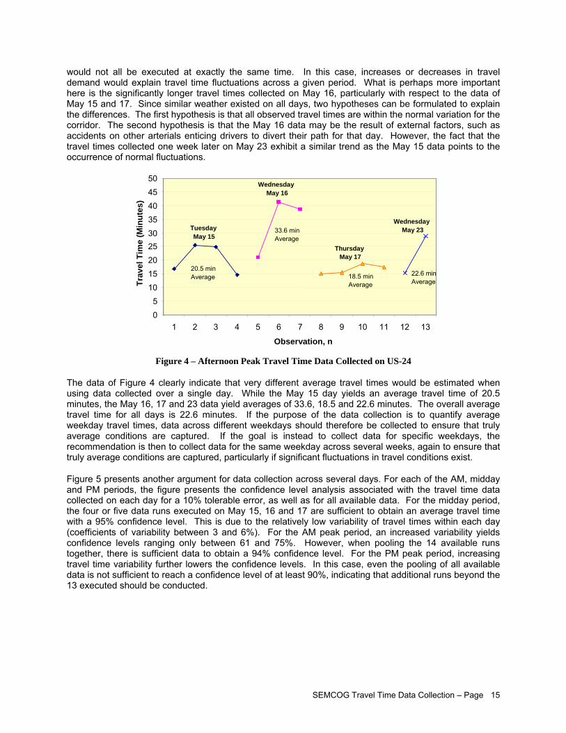
SEMCOG Travel Time Data Collection – Page 15
would not all be executed at exactly the same time. In this case, increases or decreases in travel demand would explain travel time fluctuations across a given period. What is perhaps more important here is the significantly longer travel times collected on May 16, particularly with respect to the data of May 15 and 17. Since similar weather existed on all days, two hypotheses can be formulated to explain the differences. The first hypothesis is that all observed travel times are within the normal variation for the corridor. The second hypothesis is that the May 16 data may be the result of external factors, such as accidents on other arterials enticing drivers to divert their path for that day. However, the fact that the travel times collected one week later on May 23 exhibit a similar trend as the May 15 data points to the occurrence of normal fluctuations.
Figure 4 – Afternoon Peak Travel Time Data Collected on US-24
The data of Figure 4 clearly indicate that very different average travel times would be estimated when using data collected over a single day. While the May 15 day yields an average travel time of 20.5 minutes, the May 16, 17 and 23 data yield averages of 33.6, 18.5 and 22.6 minutes. The overall average travel time for all days is 22.6 minutes. If the purpose of the data collection is to quantify average weekday travel times, data across different weekdays should therefore be collected to ensure that truly average conditions are captured. If the goal is instead to collect data for specific weekdays, the recommendation is then to collect data for the same weekday across several weeks, again to ensure that truly average conditions are captured, particularly if significant fluctuations in travel conditions exist.
Figure 5 presents another argument for data collection across several days. For each of the AM, midday and PM periods, the figure presents the confidence level analysis associated with the travel time data collected on each day for a 10% tolerable error, as well as for all available data. For the midday period, the four or five data runs executed on May 15, 16 and 17 are sufficient to obtain an average travel time with a 95% confidence level. This is due to the relatively low variability of travel times within each day (coefficients of variability between 3 and 6%). For the AM peak period, an increased variability yields confidence levels ranging only between 61 and 75%. However, when pooling the 14 available runs together, there is sufficient data to obtain a 94% confidence level. For the PM peak period, increasing travel time variability further lowers the confidence levels. In this case, even the pooling of all available data is not sufficient to reach a confidence level of at least 90%, indicating that additional runs beyond the 13 executed should be conducted.
0 5
10 15 20 25 30 35 40 45 50
1 2 3 4 5 6 7 8 9 10 11 12 13 Observation, n
Trav
el T
ime
(Min
utes
)
Tuesday May 15
Wednesday May 23
ThursdayMay 17
WednesdayMay 16
20.5 minAverage
33.6 minAverage
18.5 minAverage
22.6 minAverage
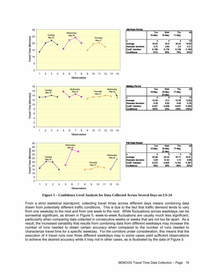
SEMCOG Travel Time Data Collection – Page 16
AM Peak PeriodTue Wed Thu All
15-May 16-May 17-May
n 4 4 4 12Average 18.63 20.6 18.04 19.09Standard deviation 3.70 3.62 2.5 3.21Coeff. Variation 0.199 0.176 0.139 0.168Confidence 61% 66% 75% 94%
Midday PeriodTue Wed Thu All
15-May 16-May 17-May23-May
n 4 5 5 14Average 13.45 13.4 13.35 13.63Standard deviation 0.36 0.52 0.49 0.76Coeff. Variation 0.027 0.039 0.037 0.056Confidence 100% 95% 100% 100%
PM Peak PeriodTue Wed Thu All
15-May 16-May 17-May23-May
n 4 5 4 13Average 20.48 29.05 16.71 22.61Standard deviation 5.58 12.93 1.74 8.98Coeff. Variation 0.272 0.445 0.104 0.397Confidence 48% 36% 85% 62%
0
5
10
15
20
25
30
1 2 3 4 5 6 7 8 9 10 11 12 13 14Observation
Trav
el T
ime
(Min
utes
) Tuesday May 15 Thursday
May 17
WednesdayMay 15
0
2
4
6
8
10
12
14
16
18
1 2 3 4 5 6 7 8 9 10 11 12 13 14Observation
Trav
el T
ime
(Min
utes
)
Tuesday May 15
WednesdayMay 23Thursday
May 17
WednesdayMay 15
05
101520253035404550
1 2 3 4 5 6 7 8 9 10 11 12 13Observation
Trav
el T
ime
(Min
utes
)
Tuesday May 15
WednesdayMay 23
ThursdayMay 17
WednesdayMay 15
AM Peak PeriodTue Wed Thu All
15-May 16-May 17-May
n 4 4 4 12Average 18.63 20.6 18.04 19.09Standard deviation 3.70 3.62 2.5 3.21Coeff. Variation 0.199 0.176 0.139 0.168Confidence 61% 66% 75% 94%
Midday PeriodTue Wed Thu All
15-May 16-May 17-May23-May
n 4 5 5 14Average 13.45 13.4 13.35 13.63Standard deviation 0.36 0.52 0.49 0.76Coeff. Variation 0.027 0.039 0.037 0.056Confidence 100% 95% 100% 100%
PM Peak PeriodTue Wed Thu All
15-May 16-May 17-May23-May
n 4 5 4 13Average 20.48 29.05 16.71 22.61Standard deviation 5.58 12.93 1.74 8.98Coeff. Variation 0.272 0.445 0.104 0.397Confidence 48% 36% 85% 62%
0
5
10
15
20
25
30
1 2 3 4 5 6 7 8
AM Peak PeriodTue Wed Thu All
15-May 16-May 17-May
n 4 4 4 12Average 18.63 20.6 18.04 19.09Standard deviation 3.70 3.62 2.5 3.21Coeff. Variation 0.199 0.176 0.139 0.168Confidence 61% 66% 75% 94%
Midday PeriodTue Wed Thu All
15-May 16-May 17-May23-May
n 4 5 5 14Average 13.45 13.4 13.35 13.63Standard deviation 0.36 0.52 0.49 0.76Coeff. Variation 0.027 0.039 0.037 0.056Confidence 100% 95% 100% 100%
PM Peak PeriodTue Wed Thu All
15-May 16-May 17-May23-May
n 4 5 4 13Average 20.48 29.05 16.71 22.61Standard deviation 5.58 12.93 1.74 8.98Coeff. Variation 0.272 0.445 0.104 0.397Confidence 48% 36% 85% 62%
0
5
10
15
20
25
30
1 2 3 4 5 6 7 8 9 10 11 12 13 14Observation
Trav
el T
ime
(Min
utes
) Tuesday May 15 Thursday
May 17
WednesdayMay 15
0
2
4
6
8
10
12
14
16
18
1 2 3 4 5 6 7 8 9 10 11 12 13 14Observation
Trav
el T
ime
(Min
utes
)
Tuesday May 15
WednesdayMay 23Thursday
May 17
WednesdayMay 15
05
101520253035404550
1 2 3 4 5 6 7 8 9 10 11 12 13Observation
Trav
el T
ime
(Min
utes
)
Tuesday May 15
WednesdayMay 23
ThursdayMay 17
WednesdayMay 15
Figure 5 – Confidence Level Analysis for Data Collected Across Several Days on US-24
From a strict statistical standpoint, collecting travel times across different days means combining data drawn from potentially different traffic conditions. This is due to the fact that traffic demand tends to vary from one weekday to the next and from one week to the next. While fluctuations across weekdays can be somewhat significant, as shown in Figure 5, week-to-week fluctuations are usually much less significant, particularly when comparing data collected in consecutive weeks or weeks that are not too far apart. As a result, the increased variability that results from combining data from different weekdays may increase the number of runs needed to obtain certain accuracy when compared to the number of runs needed to characterize travel time for a specific weekday. For the corridors under consideration, this means that the execution of 4 travel runs over three different weekdays may in some cases yield sufficient observations to achieve the desired accuracy while it may not in other cases, as is illustrated by the data of Figure 5.
SEMCOG Travel Time Data Collection – Page 17
5.5 Absolute Minimum Number of Runs to Execute
The minimum number of travel time runs to be executed for a road segment depends on the selected tolerable error, selected confidence level and typical degree of variation of travel times on the segment being surveyed.
According to NCHRP Report 398, representative sample sizes to achieve 95% confidence with a 5% allowable error using the floating car technique typically vary between 14 and 35 observations for arterials and 13 to 45 observations for freeways. These are upper limits, as lower confidence levels and higher tolerable errors can be used. In many cases, application of Equations 3 and 4 will lead to significantly lower estimates of the number of runs needed, particularly if travel times are relatively constant. Regardless of the situation, it is strongly recommended in NCHRP Report 398 that a minimum of 5 to 6 runs should be made in each direction of travel for data collection to account for potential variability associated with individual driver behavior, lane choices and random events. Variability created by such factors could be present even if care is taken to collect data in the absence of unusual events affecting traffic conditions.
5.6 Recommended Approach
Based on the survey of practice and the preliminary data analysis conducted in this section, it is recommended that use of default average coefficients of variation to characterize travel times on roadway segments to survey be considered as preliminary estimates of a minimum number of travel time runs to execute. As soon as field data is available, this information should replace any default of average value previously assumed.
Without any specific justification for higher or lower values, travel time data should be collected with the objective of estimating average travel times at a 90% confidence level with a 10% allowable error. A higher confidence level and a lower tolerable error could be used for specific operational analysis, such as before/after evaluations.
Initial requirements for this project are to conduct a minimum of 4 runs per day over three different weekdays, for a total of at least 12 runs. As indicated by the preliminary data of Tables 8 and 9, this is likely to be sufficient for a majority of segments to achieve desired accuracy in estimating weekly average travel times. This is also consistent with other documented travel time studies. For segments with significant variability in travel times, executing 12 runs may not be sufficient to adequately characterize travel conditions even if precautions are made to ensure that data collection only occurs during normal traffic conditions. For these segments, methods presented in Section 7 should be followed to determine the actual minimum number of runs needed. The governing factor determining the number of round-trip runs required on a corridor is the direction of travel requiring the highest number of runs, i.e. if NB requires 8 runs and SB requires 4 runs, you will need to perform 8 round-trip runs.
SEMCOG Travel Time Data Collection – Page 18
6 Selection of Survey Corridors and Study Segments
Selection of roadway segments to survey should depend on the purpose of the study. If the purpose is to assess traffic conditions in relation to a local development or point of interest, data collection efforts would then primarily focus on the major arterials carrying traffic to and from the site of interest. In such case, a relatively small number of roadway segments would then typically be selected for data collection. However, if the objective is to characterize traffic conditions of an entire region, all major travel corridors within the area would then be candidates for data collection. For such, a plan would need to be developed to obtain travel time data from a representative sample of roadway segments.
Elements pertaining to the identification of study corridors to survey discussed in this section include:
• Definition of geographic boundary of study • Selection of a network stratification approach • Identification of corridors • Corridor segmentation • Determination of number of segments to survey within network • Segment sample selection
6.1 Definition of Geographic Boundary
The first step of any travel time study is to define its geographical boundaries. This is important as the size of the study area affects the procedures used for selecting representative roadway samples. If a study is relatively small in scope, such as covering only a limited number of short roadway sections in the vicinity of a planned transportation improvement, it is then likely that travel data could be collected on all segments within the survey area and that no particular sampling technique would be needed. However, if the study encompasses a much larger network, such as the entire primary transportation network of an urban area, it is then unlikely that available resources would allow collecting travel data from all roadways. In this case, there would be a need to develop sampling schemes to identify reasonable groups of segments to survey for satisfying the needs of the study.
6.2 Selection of a Network Stratification
Following identification of the geographic boundary, the development of a travel time study generally focuses on the identification of types of roadways to be surveyed. For instance, travel surveys executed by transportation agencies often focus on major travel corridors. To implement such a focus, decisions are for instance often made to arbitrarily restrict data collection to freeways, expressways, major arterials and minor arterials while ignoring collectors and local streets due to their decreased role in providing mobility of throughput.
The classification scheme to be used in a particular study depends on the primary purpose of the study. In most cases, a classification scheme linked to the functional use of a similar road is used. For instance, studies conducted for planning purposes often follow classifications corresponding to the one used by local transportation planners. If the data is instead primarily collected for use in congestion management systems, functional classifications reflecting the roadway categorization used in HPMS (FHWA, 2005) or the Highway Capacity Manual 2000 (TRB, 2000) are instead favored.
Regardless of the adopted classification scheme, the specific scheme being used should result in homogeneous segment groupings, i.e., groupings in which all segments belonging to a category exhibit similar traffic and operating characteristics. As detailed in the following sections, this is to facilitate the application of sampling techniques within each group, as parameters characterizing segments within homogeneous groups will tend to have smaller variations, which then result in a need for smaller sample sizes.
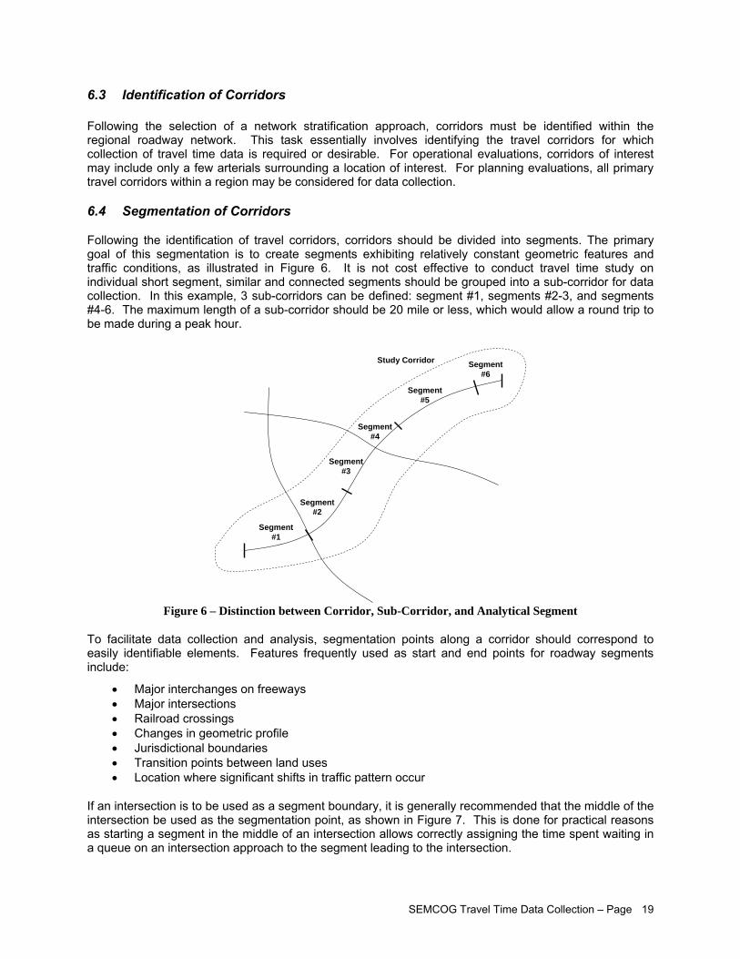
SEMCOG Travel Time Data Collection – Page 19
6.3 Identification of Corridors Following the selection of a network stratification approach, corridors must be identified within the regional roadway network. This task essentially involves identifying the travel corridors for which collection of travel time data is required or desirable. For operational evaluations, corridors of interest may include only a few arterials surrounding a location of interest. For planning evaluations, all primary travel corridors within a region may be considered for data collection.
6.4 Segmentation of Corridors
Following the identification of travel corridors, corridors should be divided into segments. The primary goal of this segmentation is to create segments exhibiting relatively constant geometric features and traffic conditions, as illustrated in Figure 6. It is not cost effective to conduct travel time study on individual short segment, similar and connected segments should be grouped into a sub-corridor for data collection. In this example, 3 sub-corridors can be defined: segment #1, segments #2-3, and segments #4-6. The maximum length of a sub-corridor should be 20 mile or less, which would allow a round trip to be made during a peak hour.
Study Corridor
Segment#1
Segment#2
Segment#3
Segment#4
Segment#5
Segment#6
Figure 6 – Distinction between Corridor, Sub-Corridor, and Analytical Segment
To facilitate data collection and analysis, segmentation points along a corridor should correspond to easily identifiable elements. Features frequently used as start and end points for roadway segments include:
• Major interchanges on freeways • Major intersections • Railroad crossings • Changes in geometric profile • Jurisdictional boundaries • Transition points between land uses • Location where significant shifts in traffic pattern occur
If an intersection is to be used as a segment boundary, it is generally recommended that the middle of the intersection be used as the segmentation point, as shown in Figure 7. This is done for practical reasons as starting a segment in the middle of an intersection allows correctly assigning the time spent waiting in a queue on an intersection approach to the segment leading to the intersection.
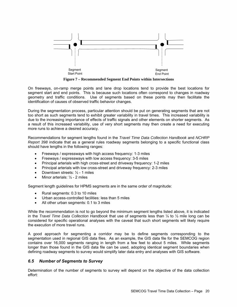
SEMCOG Travel Time Data Collection – Page 20
Figure 7 – Recommended Segment End Points within Intersections
On freeways, on-ramp merge points and lane drop locations tend to provide the best locations for segment start and end points. This is because such locations often correspond to changes in roadway geometry and traffic conditions. Use of segments based on these points may then facilitate the identification of causes of observed traffic behavior changes.
During the segmentation process, particular attention should be put on generating segments that are not too short as such segments tend to exhibit greater variability in travel times. This increased variability is due to the increasing importance of effects of traffic signals and other elements on shorter segments. As a result of this increased variability, use of very short segments may then create a need for executing more runs to achieve a desired accuracy.
Recommendations for segment lengths found in the Travel Time Data Collection Handbook and NCHRP Report 398 indicate that as a general rules roadway segments belonging to a specific functional class should have lengths in the following ranges:
• Freeways / expressways with high access frequency: 1-3 miles • Freeways / expressways with low access frequency: 3-5 miles • Principal arterials with high cross-street and driveway frequency: 1-2 miles • Principal arterials with low cross-street and driveway frequency: 2-3 miles • Downtown streets: ½ - 1 miles • Minor arterials: ½ - 2 miles
Segment length guidelines for HPMS segments are in the same order of magnitude:
• Rural segments: 0.3 to 10 miles • Urban access-controlled facilities: less than 5 miles • All other urban segments: 0.1 to 3 miles
While the recommendation is not to go beyond the minimum segment lengths listed above, it is indicated in the Travel Time Data Collection Handbook that use of segments less than ¼ to ½ mile long can be considered for specific operational analyses with the caveat that such short segments will likely require the execution of more travel runs. A good approach for segmenting a corridor may be to define segments corresponding to the segmentation used in regional GIS data files. As an example, the GIS data file for the SEMCOG region contains over 16,000 segments ranging in length from a few feet to about 5 miles. While segments longer than those found in the GIS data file can be used, adopting identical segment boundaries when defining roadway segments to survey would simplify later data entry and analyses with GIS software.
6.5 Number of Segments to Survey
Determination of the number of segments to survey will depend on the objective of the data collection effort:
Segment Start Point
Segment End Point
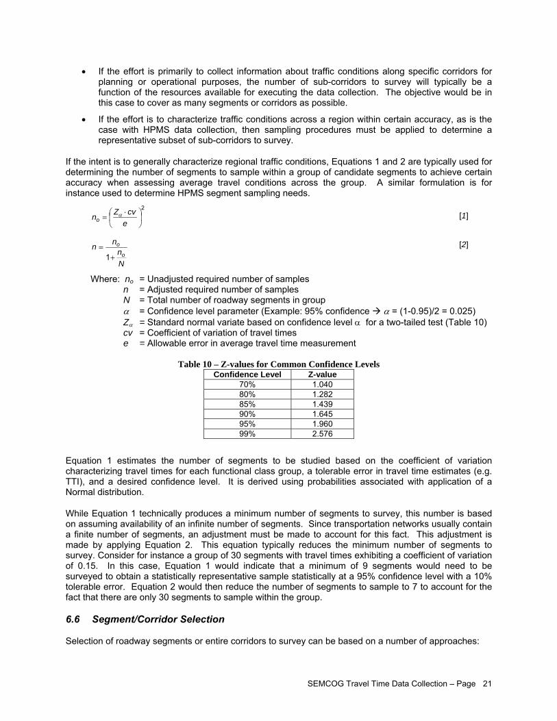
SEMCOG Travel Time Data Collection – Page 21
• If the effort is primarily to collect information about traffic conditions along specific corridors for planning or operational purposes, the number of sub-corridors to survey will typically be a function of the resources available for executing the data collection. The objective would be in this case to cover as many segments or corridors as possible.
• If the effort is to characterize traffic conditions across a region within certain accuracy, as is the case with HPMS data collection, then sampling procedures must be applied to determine a representative subset of sub-corridors to survey.
If the intent is to generally characterize regional traffic conditions, Equations 1 and 2 are typically used for determining the number of segments to sample within a group of candidate segments to achieve certain accuracy when assessing average travel conditions across the group. A similar formulation is for instance used to determine HPMS segment sampling needs.
2
⎟⎠
⎞⎜⎝
⎛ ⋅=
ecvZno
α [1]
Nn
nno
o
+=
1 [2]
Where: no = Unadjusted required number of samples n = Adjusted required number of samples N = Total number of roadway segments in group α = Confidence level parameter (Example: 95% confidence α = (1-0.95)/2 = 0.025) Zα = Standard normal variate based on confidence level α for a two-tailed test (Table 10) cv = Coefficient of variation of travel times e = Allowable error in average travel time measurement
Table 10 – Z-values for Common Confidence Levels Confidence Level Z-value
70% 1.040 80% 1.282 85% 1.439 90% 1.645 95% 1.960 99% 2.576
Equation 1 estimates the number of segments to be studied based on the coefficient of variation characterizing travel times for each functional class group, a tolerable error in travel time estimates (e.g. TTI), and a desired confidence level. It is derived using probabilities associated with application of a Normal distribution.
While Equation 1 technically produces a minimum number of segments to survey, this number is based on assuming availability of an infinite number of segments. Since transportation networks usually contain a finite number of segments, an adjustment must be made to account for this fact. This adjustment is made by applying Equation 2. This equation typically reduces the minimum number of segments to survey. Consider for instance a group of 30 segments with travel times exhibiting a coefficient of variation of 0.15. In this case, Equation 1 would indicate that a minimum of 9 segments would need to be surveyed to obtain a statistically representative sample statistically at a 95% confidence level with a 10% tolerable error. Equation 2 would then reduce the number of segments to sample to 7 to account for the fact that there are only 30 segments to sample within the group.
6.6 Segment/Corridor Selection
Selection of roadway segments or entire corridors to survey can be based on a number of approaches:
SEMCOG Travel Time Data Collection – Page 22
• Random sampling. Random selection of roadway segments across the survey area.
• Stratified random sampling. In this approach, the group of segments to survey is divided into a number of categories. The number of segments to survey within each category is then determined, followed by a random selection of specific segments to survey within each category.
• Prioritized random sampling. In this approach, a certain fraction of segments to survey is selected based on one or more specific criteria, while the remaining segments are randomly selected. For instance, the selection process could be set so that the five or ten most congested roadway segments are always selected, with the remaining segments needed to satisfy minimum sampling requirements randomly selected among the remaining candidates.
• Criteria-based sampling. Selection of all segments to survey based solely on the application of predefined criteria.
• Arbitrary sampling. Selection of all segments to survey based only on professional judgment.
While a random sampling approach conceptually follows statistical rigor, it tends to increase data collection costs by scattering segments to survey and increasing the distance required to travel to and from each segment. For this reason, use of alternative selection methods is usually preferred when limited resources constrain the data collection effort.
A stratified random sampling approach is used in HPMS to identify the segments to be surveyed (FHWA, 2005). This approach first divides roadway segments within a network based on the environment: urban areas, small urban areas and rural areas. For each area, segments are then grouped based on their annual average daily traffic (AADT). For instance, principal arterials in small urban areas with AADTs between 0 and 5000 are classified into a first group, arterials with AADTs between 5,000 and 10,000 into a second group, arterials with AADTs between 10,000 and 15,000 into a third group, and so on. This stratification allows segments with relatively similar characteristics to be grouped together and tends to reduce the number of segments needed within each group to achieve certain sampling accuracy. The number of segments to sample within each group is then determined using Equations 1 and 2, with specific segments to survey within each group selected according to a random process. While it is acknowledged that this approach is not theoretically the best to collect sample data, it is viewed as an acceptable compromise between statistical rigor and the need to develop a data collection procedure that must be simple and cost efficient to meet certain manpower and cost considerations.
The Travel Time Data Collection Handbook favors application of the prioritized sampling approach. In this case, the suggestion is to identify congested or critical segments as high priority and draw specifically 10 to 20% of the total number of segments to survey from the high-priority group. The rationale for this approach is based on the benefits it provides when applied as part of a multi-year data collection program. For instance, repetitive application of the prioritized sampling approach ensures that critical segments are surveyed frequently, if not every year, while allowing less critical segments to be surveyed on a less frequent basis. Similar to the stratified approach, while it is acknowledged that prioritized sampling may not conform to thorough statistical rigor, it is recognized that such an approach allows data collection efforts to concentrate on the most critical locations and tend to a more efficient use of available resources when considering the reasons for which travel time surveys are usually conducted.
Selection simply based on the application of selection criteria or engineering judgment is usually not recommended as such approaches do not guarantee the creation of non-biased samples. In both cases, selection is heavily influenced by the judgment of the person, or persons, selecting the sampling criteria or performing the selection. While all efforts may be put to select relevant criterion or segments, there is no guarantee that specific categories of segment may end up being over- or under-represented.
6.7 Recommended Approach
Based on elements discussed in the previous section, the following approach is recommended for selecting roadway segments for annual travel time study:
SEMCOG Travel Time Data Collection – Page 23
• STEP 1 – Define geographical boundaries of the network considered for data collection.
• STEP 2 – Stratify roadways within the survey area into major functional class groups:
o Freeways o Arterials
• STEP 3 – Identify travel corridors within roadway
• STEP 4 – Divide each identified corridor into segments having homogenous characteristics in terms of land use, roadway geometry, cross-section features, and speed limits
o Freeways / expressways High access frequency: 1-3 miles Low access frequency: 3-5 miles
o Principal arterials High cross-street and driveway frequency: 1-2 miles Low cross-street and driveway frequency: 2-3 miles
o Downtown streets: ½ - 1 miles
o Minor arterials: ½ - 2 miles
• STEP 5 – Determine number of cluster segments to survey within each group
o If the intent is to survey specific corridors for planning/operational purposes, identify number of miles that can be surveyed based on available resources.
o If the intent is to characterize regional travel conditions through statistical sampling, use Equations 1 and 2 described in Section 6.5 to determine the number of segments that need to be surveyed within each functional class group to achieve desired accuracy. This will require determining a typical coefficient of variation of travel time on the type of facility being considered (see Section 5.1), an allowable error (see Section 5.2), and a confidence level (See Section 5.3).
• STEP 6 – Select cluster segments to survey within each functional group
o Selection should start with the high priority corridors. Either all identified high priority corridors can be selected until all available resources are assigned or an arbitrary fraction of segments (for instance 20%) could be selected.
o If resources are still available after selection of high priority corridors, non-priority corridors can be randomly selected until the minimum number of segments to survey within each functional category has been met.
6.8 Recommended Regional Travel Time Monitoring Program
One of the most important steps in the implementation of Congestion Management Process is monitoring the traffic congestion on a regular basis. Travel time is a direct measurement of congestion. SEMCOG should establish an annual program to collect travel time data and track the regional Travel Time Index (TTI). Travel time data can be collected on selected segments using the statistical sampling approach developed in this report. The TTI will provide the regional stakeholders with an objective and quantitative assessment of the current conditions and trend of traffic congestion.
Travel Time Index (TTI) is the ratio of actual travel time to free flow travel time. The TTI indicates the average amount of extra time it takes to travel relative to the free-flow travel. A TTI of 1.2, for example, indicates that a 30-minute free-flow trip will take 36 minutes during the peak hour period, or a 20% delay
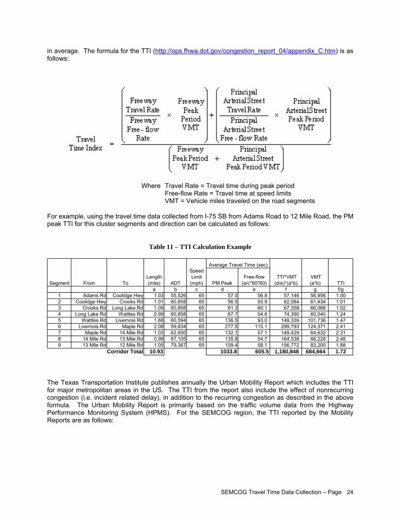
SEMCOG Travel Time Data Collection – Page 24
in average. The formula for the TTI (http://ops.fhwa.dot.gov/congestion_report_04/appendix_C.htm) is as follows:
Where Travel Rate = Travel time during peak period Free-flow Rate = Travel time at speed limits VMT = Vehicle miles traveled on the road segments
For example, using the travel time data collected from I-75 SB from Adams Road to 12 Mile Road, the PM peak TTI for this cluster segments and direction can be calculated as follows:
Table 11 – TTI Calculation Example
PM PeakFree-flow
(a/c*60*60)a b c d e f g f/g
1 Adams Rd Coolidge Hwy 1.03 55,526 65 57.0 56.8 57,146 56,956 1.002 Coolidge Hwy Crooks Rd 1.01 60,858 65 56.5 55.9 62,084 61,434 1.013 Crooks Rd Long Lake Rd 1.09 60,858 65 61.3 60.1 67,358 66,068 1.024 Long Lake Rd Wattles Rd 0.99 60,858 65 67.7 54.6 74,390 60,040 1.245 Wattles Rd Livernois Rd 1.68 60,594 65 136.5 93.0 149,339 101,736 1.476 Livernois Rd Maple Rd 2.08 59,834 65 277.5 115.1 299,793 124,371 2.417 Maple Rd 14 Mile Rd 1.03 62,650 65 132.1 57.1 149,429 64,632 2.318 14 Mile Rd 13 Mile Rd 0.99 67,105 65 135.8 54.7 164,538 66,228 2.489 13 Mile Rd 12 Mile Rd 1.05 79,367 65 109.4 58.1 156,772 83,200 1.88
10.93 1033.8 605.5 1,180,848 684,664 1.72
To
Speed Limit (mph)
VMT (a*b)
Average Travel Time (sec)
ADTLength (mile) TTI
Corridor Total
FromSegment TTI*VMT (d/e)*(a*b)
The Texas Transportation Institute publishes annually the Urban Mobility Report which includes the TTI for major metropolitan areas in the US. The TTI from the report also include the effect of nonrecurring congestion (i.e. incident related delay), in addition to the recurring congestion as described in the above formula. The Urban Mobility Report is primarily based on the traffic volume data from the Highway Performance Monitoring System (HPMS). For the SEMCOG region, the TTI reported by the Mobility Reports are as follows:
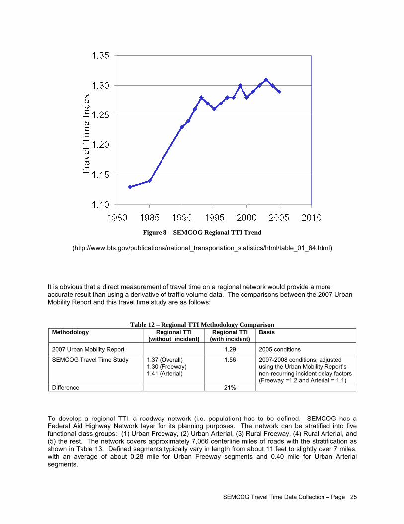
SEMCOG Travel Time Data Collection – Page 25
Figure 8 – SEMCOG Regional TTI Trend
(http://www.bts.gov/publications/national_transportation_statistics/html/table_01_64.html)
It is obvious that a direct measurement of travel time on a regional network would provide a more accurate result than using a derivative of traffic volume data. The comparisons between the 2007 Urban Mobility Report and this travel time study are as follows:
Table 12 – Regional TTI Methodology Comparison Methodology Regional TTI
(without incident) Regional TTI
(with incident) Basis
2007 Urban Mobility Report 1.29 2005 conditions
SEMCOG Travel Time Study 1.37 (Overall) 1.30 (Freeway) 1.41 (Arterial)
1.56 2007-2008 conditions, adjusted using the Urban Mobility Report’s non-recurring incident delay factors (Freeway =1.2 and Arterial = 1.1)
Difference 21%
To develop a regional TTI, a roadway network (i.e. population) has to be defined. SEMCOG has a Federal Aid Highway Network layer for its planning purposes. The network can be stratified into five functional class groups: (1) Urban Freeway, (2) Urban Arterial, (3) Rural Freeway, (4) Rural Arterial, and (5) the rest. The network covers approximately 7,066 centerline miles of roads with the stratification as shown in Table 13. Defined segments typically vary in length from about 11 feet to slightly over 7 miles, with an average of about 0.28 mile for Urban Freeway segments and 0.40 mile for Urban Arterial segments.
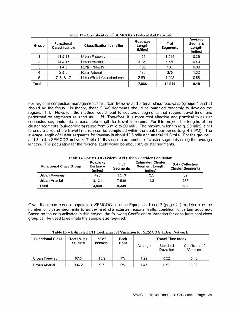
SEMCOG Travel Time Data Collection – Page 26
Table 13 – Stratification of SEMCOG’s Federal Aid Network
Group Functional Classification Classification Identifier
Roadway Length (Miles)
# of Segments
Average Segment Length (miles)
1 11 & 12 Urban Freeway 423 1,519 0.28 2 14 & 16 Urban Arterial 3,121 7,830 0.40 3 1 & 5 Rural Freeway 136 137 0.99 4 2 & 6 Rural Arterial 495 375 1.32 5 7, 8, & 17 Urban/Rural Collector/Local 2,891 4,998 0.58
Total 7,066 14,859 0.48
For regional congestion management, the urban freeway and arterial class roadways (groups 1 and 2) should be the focus. In theory, these 9,349 segments should be sampled randomly to develop the regional TTI. However, the method would lead to scattered segments that require travel time runs performed on segments as short as 11 ft! Therefore, it is more cost effective and practical to cluster connected segments into a reasonable length for travel time runs. For this project, the lengths of the cluster segments (sub-corridors) range from 5 mile to 20 mile. The maximum length (e.g. 20 mile) is set to ensure a round trip travel time run can be completed within the peak hour period (e.g. 4-6 PM). The average length of cluster segments for freeway is about 13.5 mile and arterial 11.3 mile. For the groups 1 and 2 in the SEMCOG network, Table 14 lists estimated number of cluster segments using the average lengths. The population for the regional study would be about 309 cluster segments.
Table 14 – SEMCOG Federal Aid Urban Corridor Population
Functional Class Group Roadway Distance (miles)
# of Segments
Estimated Cluster Segment Length
(miles) Data Collection
Cluster Segments
Urban Freeway 423 1,519 13.5 32 Urban Arterial 3,121 7,830 11.3 277 Total 3,544 9,349 309
Given the urban corridor population, SEMCOG can use Equations 1 and 2 (page 21) to determine the number of cluster segments to survey and characterize regional traffic condition to certain accuracy. Based on the data collected in this project, the following Coefficient of Variation for each functional class group can be used to estimate the sample size required:
Table 15 – Estimated TTI Coefficient of Variation for SEMCOG Urban Network
Travel Time Index Functional Class Total Miles Studied
% of network
Peak Hour
Average Standard Deviation
Coefficient of Variation
Urban Freeway 67.3 15.9 PM 1.29 0.52 0.40
Urban Arterial 304.2 9.7 PM 1.47 0.51 0.35
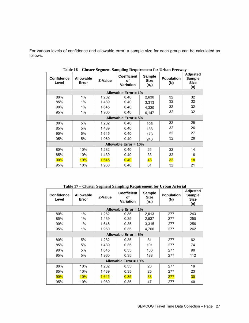
SEMCOG Travel Time Data Collection – Page 27
For various levels of confidence and allowable error, a sample size for each group can be calculated as follows.
Table 16 – Cluster Segment Sampling Requirement for Urban Freeway
Confidence Level
Allowable Error Z-Value
Coefficient of
Variation
Sample Size (no)
Population (N)
Adjusted Sample
Size (n)
Allowable Error = 1% 80% 1% 1.282 0.40 2,630 32 32 85% 1% 1.439 0.40 3,313 32 32 90% 1% 1.645 0.40 4,330 32 32 95% 1% 1.960 0.40 6,147 32 32
Allowable Error = 5% 80% 5% 1.282 0.40 105 32 25 85% 5% 1.439 0.40 133 32 26 90% 5% 1.645 0.40 173 32 27 95% 5% 1.960 0.40 246 32 28
Allowable Error = 10% 80% 10% 1.282 0.40 26 32 14 85% 10% 1.439 0.40 33 32 16 90% 10% 1.645 0.40 43 32 18 95% 10% 1.960 0.40 61 32 21
Table 17 – Cluster Segment Sampling Requirement for Urban Arterial
Confidence Level
Allowable Error Z-Value
Coefficient of
Variation
Sample Size (no)
Population (N)
Adjusted Sample
Size (n)
Allowable Error = 1% 80% 1% 1.282 0.35 2,013 277 243 85% 1% 1.439 0.35 2,537 277 250 90% 1% 1.645 0.35 3,315 277 256 95% 1% 1.960 0.35 4,706 277 262
Allowable Error = 5% 80% 5% 1.282 0.35 81 277 62 85% 5% 1.439 0.35 101 277 74 90% 5% 1.645 0.35 133 277 90 95% 5% 1.960 0.35 188 277 112
Allowable Error = 10% 80% 10% 1.282 0.35 20 277 19 85% 10% 1.439 0.35 25 277 23 90% 10% 1.645 0.35 33 277 30 95% 10% 1.960 0.35 47 277 40
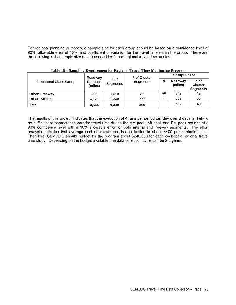
SEMCOG Travel Time Data Collection – Page 28
For regional planning purposes, a sample size for each group should be based on a confidence level of 90%, allowable error of 10%, and coefficient of variation for the travel time within the group. Therefore, the following is the sample size recommended for future regional travel time studies:
Table 18 – Sampling Requirement for Regional Travel Time Monitoring Program
Sample Size Functional Class Group
Roadway Distance (miles)
# of Segments
# of Cluster Segments
% Roadway
(miles) # of
Cluster Segments
Urban Freeway 423 1,519 32 56 243 18 Urban Arterial 3,121 7,830 277 11 339 30
Total 3,544 9,349 309 582 48
The results of this project indicates that the execution of 4 runs per period per day over 3 days is likely to be sufficient to characterize corridor travel time during the AM peak, off-peak and PM peak periods at a 90% confidence level with a 10% allowable error for both arterial and freeway segments. The effort analysis indicates that average cost of travel time data collection is about $400 per centerline mile. Therefore, SEMCOG should budget for the program about $240,000 for each cycle of a regional travel time study. Depending on the budget available, the data collection cycle can be 2-3 years.
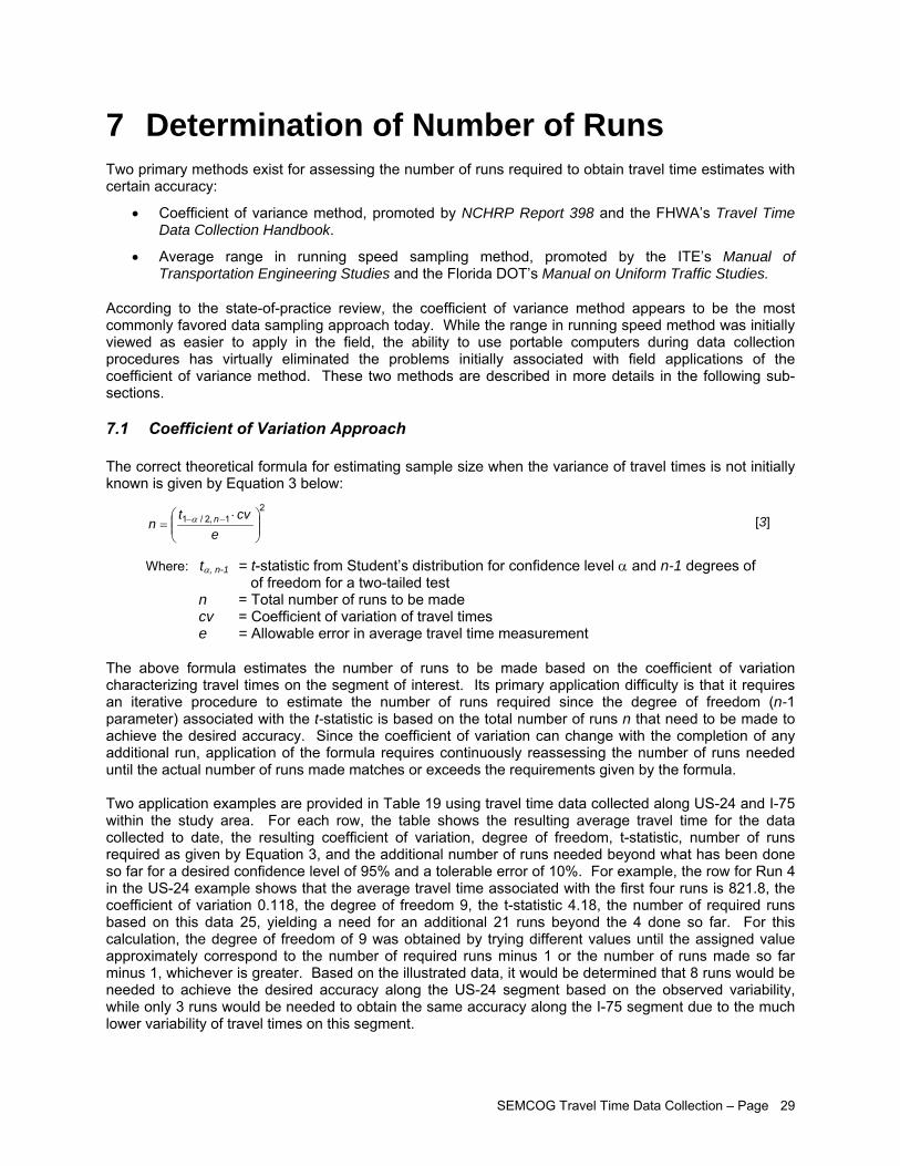
SEMCOG Travel Time Data Collection – Page 29
7 Determination of Number of Runs Two primary methods exist for assessing the number of runs required to obtain travel time estimates with certain accuracy:
• Coefficient of variance method, promoted by NCHRP Report 398 and the FHWA’s Travel Time Data Collection Handbook.
• Average range in running speed sampling method, promoted by the ITE’s Manual of Transportation Engineering Studies and the Florida DOT’s Manual on Uniform Traffic Studies.
According to the state-of-practice review, the coefficient of variance method appears to be the most commonly favored data sampling approach today. While the range in running speed method was initially viewed as easier to apply in the field, the ability to use portable computers during data collection procedures has virtually eliminated the problems initially associated with field applications of the coefficient of variance method. These two methods are described in more details in the following sub-sections.
7.1 Coefficient of Variation Approach The correct theoretical formula for estimating sample size when the variance of travel times is not initially known is given by Equation 3 below:
21 ,2/1
⎟⎟⎠
⎞⎜⎜⎝
⎛ ⋅= −−
ecvt
n nα [3]
Where: tα, n-1 = t-statistic from Student’s distribution for confidence level α and n-1 degrees of of freedom for a two-tailed test n = Total number of runs to be made cv = Coefficient of variation of travel times e = Allowable error in average travel time measurement
The above formula estimates the number of runs to be made based on the coefficient of variation characterizing travel times on the segment of interest. Its primary application difficulty is that it requires an iterative procedure to estimate the number of runs required since the degree of freedom (n-1 parameter) associated with the t-statistic is based on the total number of runs n that need to be made to achieve the desired accuracy. Since the coefficient of variation can change with the completion of any additional run, application of the formula requires continuously reassessing the number of runs needed until the actual number of runs made matches or exceeds the requirements given by the formula. Two application examples are provided in Table 19 using travel time data collected along US-24 and I-75 within the study area. For each row, the table shows the resulting average travel time for the data collected to date, the resulting coefficient of variation, degree of freedom, t-statistic, number of runs required as given by Equation 3, and the additional number of runs needed beyond what has been done so far for a desired confidence level of 95% and a tolerable error of 10%. For example, the row for Run 4 in the US-24 example shows that the average travel time associated with the first four runs is 821.8, the coefficient of variation 0.118, the degree of freedom 9, the t-statistic 4.18, the number of required runs based on this data 25, yielding a need for an additional 21 runs beyond the 4 done so far. For this calculation, the degree of freedom of 9 was obtained by trying different values until the assigned value approximately correspond to the number of required runs minus 1 or the number of runs made so far minus 1, whichever is greater. Based on the illustrated data, it would be determined that 8 runs would be needed to achieve the desired accuracy along the US-24 segment based on the observed variability, while only 3 runs would be needed to obtain the same accuracy along the I-75 segment due to the much lower variability of travel times on this segment.
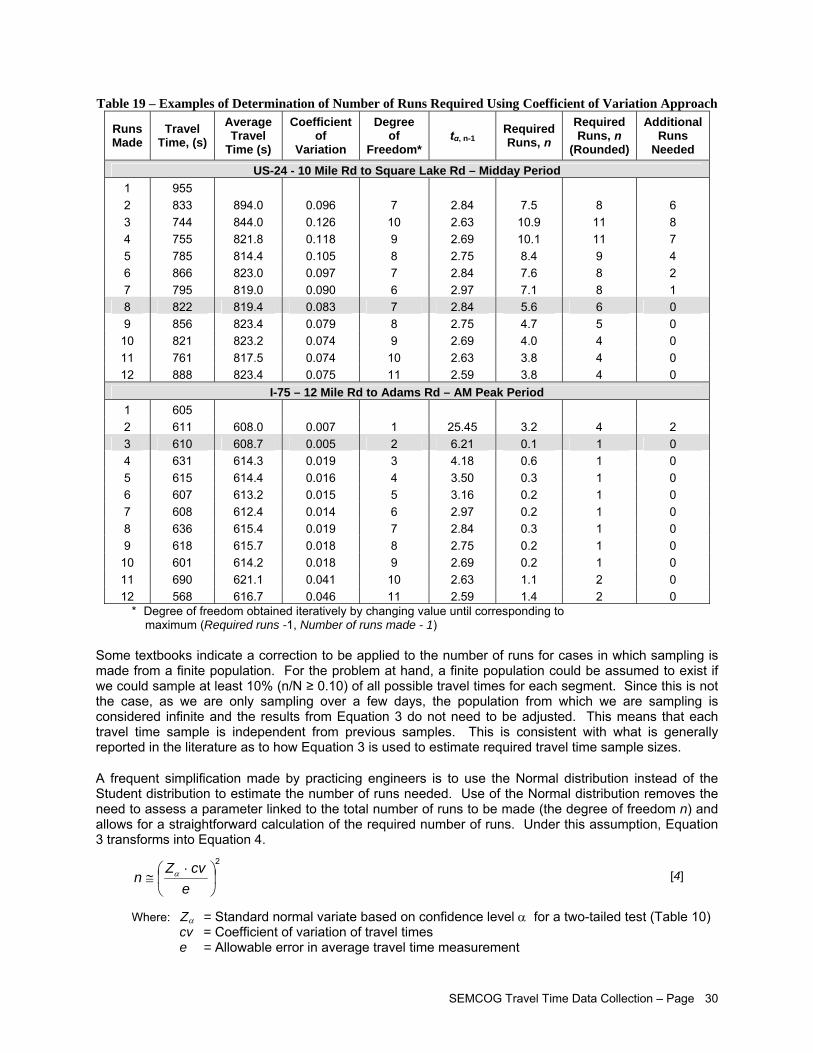
SEMCOG Travel Time Data Collection – Page 30
Table 19 – Examples of Determination of Number of Runs Required Using Coefficient of Variation Approach
Runs Made
Travel Time, (s)
Average Travel
Time (s)
Coefficient of
Variation
Degree of
Freedom* tα, n-1 Required
Runs, n Required Runs, n
(Rounded)
Additional Runs
Needed
US-24 - 10 Mile Rd to Square Lake Rd – Midday Period 1 955 2 833 894.0 0.096 7 2.84 7.5 8 6 3 744 844.0 0.126 10 2.63 10.9 11 8 4 755 821.8 0.118 9 2.69 10.1 11 7 5 785 814.4 0.105 8 2.75 8.4 9 4 6 866 823.0 0.097 7 2.84 7.6 8 2 7 795 819.0 0.090 6 2.97 7.1 8 1 8 822 819.4 0.083 7 2.84 5.6 6 0 9 856 823.4 0.079 8 2.75 4.7 5 0
10 821 823.2 0.074 9 2.69 4.0 4 0 11 761 817.5 0.074 10 2.63 3.8 4 0 12 888 823.4 0.075 11 2.59 3.8 4 0
I-75 – 12 Mile Rd to Adams Rd – AM Peak Period 1 605 2 611 608.0 0.007 1 25.45 3.2 4 2 3 610 608.7 0.005 2 6.21 0.1 1 0 4 631 614.3 0.019 3 4.18 0.6 1 0 5 615 614.4 0.016 4 3.50 0.3 1 0 6 607 613.2 0.015 5 3.16 0.2 1 0 7 608 612.4 0.014 6 2.97 0.2 1 0 8 636 615.4 0.019 7 2.84 0.3 1 0 9 618 615.7 0.018 8 2.75 0.2 1 0
10 601 614.2 0.018 9 2.69 0.2 1 0 11 690 621.1 0.041 10 2.63 1.1 2 0 12 568 616.7 0.046 11 2.59 1.4 2 0
* Degree of freedom obtained iteratively by changing value until corresponding to maximum (Required runs -1, Number of runs made - 1)
Some textbooks indicate a correction to be applied to the number of runs for cases in which sampling is made from a finite population. For the problem at hand, a finite population could be assumed to exist if we could sample at least 10% (n/N ≥ 0.10) of all possible travel times for each segment. Since this is not the case, as we are only sampling over a few days, the population from which we are sampling is considered infinite and the results from Equation 3 do not need to be adjusted. This means that each travel time sample is independent from previous samples. This is consistent with what is generally reported in the literature as to how Equation 3 is used to estimate required travel time sample sizes.
A frequent simplification made by practicing engineers is to use the Normal distribution instead of the Student distribution to estimate the number of runs needed. Use of the Normal distribution removes the need to assess a parameter linked to the total number of runs to be made (the degree of freedom n) and allows for a straightforward calculation of the required number of runs. Under this assumption, Equation 3 transforms into Equation 4.
2
⎟⎠
⎞⎜⎝
⎛ ⋅≅
ecvZn α [4]
Where: Zα = Standard normal variate based on confidence level α for a two-tailed test (Table 10) cv = Coefficient of variation of travel times e = Allowable error in average travel time measurement
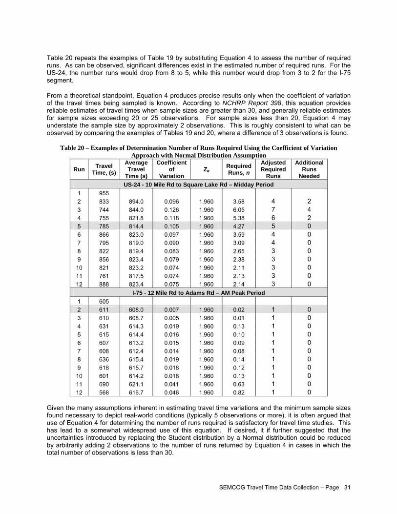
SEMCOG Travel Time Data Collection – Page 31
Table 20 repeats the examples of Table 19 by substituting Equation 4 to assess the number of required runs. As can be observed, significant differences exist in the estimated number of required runs. For the US-24, the number runs would drop from 8 to 5, while this number would drop from 3 to 2 for the I-75 segment.
From a theoretical standpoint, Equation 4 produces precise results only when the coefficient of variation of the travel times being sampled is known. According to NCHRP Report 398, this equation provides reliable estimates of travel times when sample sizes are greater than 30, and generally reliable estimates for sample sizes exceeding 20 or 25 observations. For sample sizes less than 20, Equation 4 may understate the sample size by approximately 2 observations. This is roughly consistent to what can be observed by comparing the examples of Tables 19 and 20, where a difference of 3 observations is found.
Table 20 – Examples of Determination Number of Runs Required Using the Coefficient of Variation Approach with Normal Distribution Assumption
Run Travel Time, (s)
Average Travel
Time (s)
Coefficient of
Variation Zα
Required Runs, n
Adjusted Required
Runs
Additional Runs
Needed US-24 - 10 Mile Rd to Square Lake Rd – Midday Period
1 955 2 833 894.0 0.096 1.960 3.58 4 2 3 744 844.0 0.126 1.960 6.05 7 4 4 755 821.8 0.118 1.960 5.38 6 2 5 785 814.4 0.105 1.960 4.27 5 0 6 866 823.0 0.097 1.960 3.59 4 0 7 795 819.0 0.090 1.960 3.09 4 0 8 822 819.4 0.083 1.960 2.65 3 0 9 856 823.4 0.079 1.960 2.38 3 0 10 821 823.2 0.074 1.960 2.11 3 0 11 761 817.5 0.074 1.960 2.13 3 0 12 888 823.4 0.075 1.960 2.14 3 0
I-75 - 12 Mile Rd to Adams Rd – AM Peak Period 1 605 2 611 608.0 0.007 1.960 0.02 1 0 3 610 608.7 0.005 1.960 0.01 1 0 4 631 614.3 0.019 1.960 0.13 1 0 5 615 614.4 0.016 1.960 0.10 1 0 6 607 613.2 0.015 1.960 0.09 1 0 7 608 612.4 0.014 1.960 0.08 1 0 8 636 615.4 0.019 1.960 0.14 1 0 9 618 615.7 0.018 1.960 0.12 1 0 10 601 614.2 0.018 1.960 0.13 1 0 11 690 621.1 0.041 1.960 0.63 1 0 12 568 616.7 0.046 1.960 0.82 1 0
Given the many assumptions inherent in estimating travel time variations and the minimum sample sizes found necessary to depict real-world conditions (typically 5 observations or more), it is often argued that use of Equation 4 for determining the number of runs required is satisfactory for travel time studies. This has lead to a somewhat widespread use of this equation. If desired, it if further suggested that the uncertainties introduced by replacing the Student distribution by a Normal distribution could be reduced by arbitrarily adding 2 observations to the number of runs returned by Equation 4 in cases in which the total number of observations is less than 30.
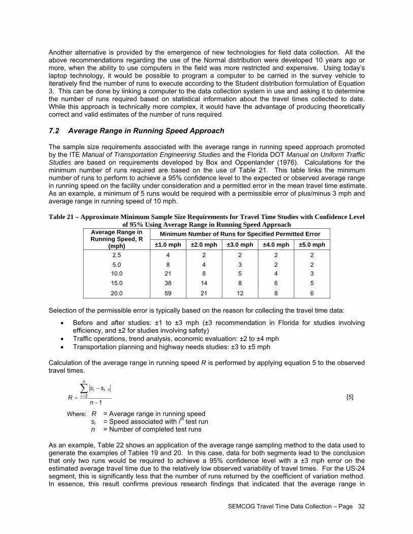
SEMCOG Travel Time Data Collection – Page 32
Another alternative is provided by the emergence of new technologies for field data collection. All the above recommendations regarding the use of the Normal distribution were developed 10 years ago or more, when the ability to use computers in the field was more restricted and expensive. Using today’s laptop technology, it would be possible to program a computer to be carried in the survey vehicle to iteratively find the number of runs to execute according to the Student distribution formulation of Equation 3. This can be done by linking a computer to the data collection system in use and asking it to determine the number of runs required based on statistical information about the travel times collected to date. While this approach is technically more complex, it would have the advantage of producing theoretically correct and valid estimates of the number of runs required.
7.2 Average Range in Running Speed Approach
The sample size requirements associated with the average range in running speed approach promoted by the ITE Manual of Transportation Engineering Studies and the Florida DOT Manual on Uniform Traffic Studies are based on requirements developed by Box and Oppenlander (1976). Calculations for the minimum number of runs required are based on the use of Table 21. This table links the minimum number of runs to perform to achieve a 95% confidence level to the expected or observed average range in running speed on the facility under consideration and a permitted error in the mean travel time estimate. As an example, a minimum of 5 runs would be required with a permissible error of plus/minus 3 mph and average range in running speed of 10 mph. Table 21 – Approximate Minimum Sample Size Requirements for Travel Time Studies with Confidence Level
of 95% Using Average Range in Running Speed Approach Minimum Number of Runs for Specified Permitted Error Average Range in
Running Speed, R (mph) ±1.0 mph ±2.0 mph ±3.0 mph ±4.0 mph ±5.0 mph
2.5 4 2 2 2 2 5.0 8 4 3 2 2 10.0 21 8 5 4 3 15.0 38 14 8 6 5
20.0 59 21 12 8 6
Selection of the permissible error is typically based on the reason for collecting the travel time data:
• Before and after studies: ±1 to ±3 mph (±3 recommendation in Florida for studies involving efficiency, and ±2 for studies involving safety)
• Traffic operations, trend analysis, economic evaluation: ±2 to ±4 mph • Transportation planning and highway needs studies: ±3 to ±5 mph
Calculation of the average range in running speed R is performed by applying equation 5 to the observed travel times.
12
1
−
−
=∑
=−
n
ssR
n
iii
[5]
Where: R = Average range in running speed si = Speed associated with ith test run n = Number of completed test runs
As an example, Table 22 shows an application of the average range sampling method to the data used to generate the examples of Tables 19 and 20. In this case, data for both segments lead to the conclusion that only two runs would be required to achieve a 95% confidence level with a ±3 mph error on the estimated average travel time due to the relatively low observed variability of travel times. For the US-24 segment, this is significantly less that the number of runs returned by the coefficient of variation method. In essence, this result confirms previous research findings that indicated that the average range in
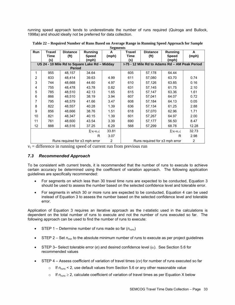
SEMCOG Travel Time Data Collection – Page 33
running speed approach tends to underestimate the number of runs required (Quiroga and Bullock, 1998a) and should ideally not be preferred for data collection.
Table 22 – Required Number of Runs Based on Average Range in Running Speed Approach for Sample Segments
Run Travel Time
(s)
Distance (ft)
Running Speed (mph)
A (mph)
Travel Time
(s)
Distance (ft)
Running Speed (mph)
A (mph)
US 24 - 10 Mile Rd to Square Lake Rd – Midday Period
I-75 - 12 Mile Rd to Adams Rd – AM Peak Period
1 955 48,157 34.64 605 57,178 64.44 2 833 48,414 39.63 4.99 611 57,080 63.70 0.74 3 744 48,668 44.60 4.97 610 57,126 63.85 0.16 4 755 48,478 43.78 0.82 631 57,145 61.75 2.10 5 785 48,510 42.13 1.65 615 57,147 63.36 1.61 6 866 48,510 38.19 3.94 607 57,041 64.07 0.72 7 795 48,579 41.66 3.47 608 57,184 64.13 0.05 8 822 48,557 40.28 1.39 636 57,134 61.25 2.88 9 856 48,666 38.76 1.51 618 57,070 62.96 1.71 10 821 48,347 40.15 1.39 601 57,267 64.97 2.00 11 761 48,600 43.54 3.39 690 57,177 56.50 8.47 12 888 48,516 37.25 6.29 568 57,299 68.78 12.28
Σ|vi-vi-1| 33.81 Σ|vi-vi-1| 32.73 R 3.07 R 2.98
Runs required for ±3 mph error 2 Runs required for ±3 mph error 2 vi = difference in running speed of current run from previous run
7.3 Recommended Approach
To be consistent with current trends, it is recommended that the number of runs to execute to achieve certain accuracy be determined using the coefficient of variation approach. The following application guidelines are specifically recommended:
• For segments on which less than 30 travel time runs are expected to be conducted, Equation 3 should be used to assess the number based on the selected confidence level and tolerable error.
• For segments in which 30 or more runs are expected to be conducted, Equation 4 can be used instead of Equation 3 to assess the number based on the selected confidence level and tolerable error.
Application of Equation 3 requires an iterative approach as the t-statistic used in the calculations is dependent on the total number of runs to execute and not the number of runs executed so far. The following approach can be used to find the number of runs to execute:
• STEP 1 – Determine number of runs made so far (nruns)
• STEP 2 – Set nmin to the absolute minimum number of runs to execute as per project guidelines
• STEP 3– Select tolerable error (e) and desired confidence level (α). See Section 5.6 for recommended values
• STEP 4 – Assess coefficient of variation of travel times (cv) for number of runs executed so far
o If nruns < 2, use default values from Section 5.6 or any other reasonable value
o If nruns ≥ 2, calculate coefficient of variation of travel times as per Equation X below
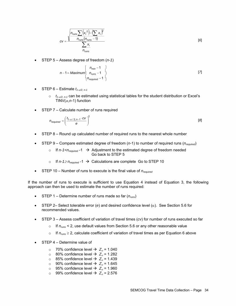
SEMCOG Travel Time Data Collection – Page 34
( ) ( )( )
runs
i
runsruns
iiruns
nx
nnxxn
cv∑
∑ ∑−
−
=1
22
[6]
• STEP 5 – Assess degree of freedom (n-1)
⎪⎭
⎪⎬
⎫
⎪⎩
⎪⎨
⎧
−−−
=−1
11
1
required
runs
min
nnn
Maximumn [7]
• STEP 6 – Estimate t1-α/2, n-1
o t1-α/2, n-1 can be estimated using statistical tables for the student distribution or Excel’s TINV(α,n-1) function
• STEP 7 – Calculate number of runs required 2
1 ,2/1⎟⎟⎠
⎞⎜⎜⎝
⎛ ⋅= −−
ecvt
n nrequired
α [8]
• STEP 8 – Round up calculated number of required runs to the nearest whole number
• STEP 9 – Compare estimated degree of freedom (n-1) to number of required runs (nrequired)
o If n-1<nrequired -1 Adjustment to the estimated degree of freedom needed Go back to STEP 5
o If n-1≥ nrequired -1 Calculations are complete Go to STEP 10
• STEP 10 – Number of runs to execute is the final value of nrequired
If the number of runs to execute is sufficient to use Equation 4 instead of Equation 3, the following approach can then be used to estimate the number of runs required:
• STEP 1 – Determine number of runs made so far (nruns)
• STEP 2– Select tolerable error (e) and desired confidence level (α). See Section 5.6 for recommended values.
• STEP 3 – Assess coefficient of variation of travel times (cv) for number of runs executed so far
o If nruns < 2, use default values from Section 5.6 or any other reasonable value
o If nruns ≥ 2, calculate coefficient of variation of travel times as per Equation 6 above
• STEP 4 – Determine value of
o 70% confidence level Zα = 1.040 o 80% confidence level Zα = 1.282 o 85% confidence level Zα = 1.439 o 90% confidence level Zα = 1.645 o 95% confidence level Zα = 1.960 o 99% confidence level Zα = 2.576

SEMCOG Travel Time Data Collection – Page 35
• STEP 5 – Calculate number of runs required as per Equation 9 below 2
⎟⎠
⎞⎜⎝
⎛ ⋅≅
ecvZnrequired
α [9]
• STEP 6 – Round up calculated number of required runs to the nearest whole number
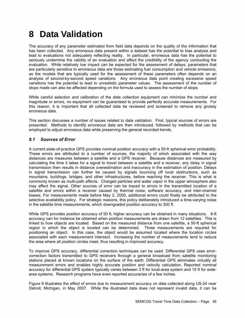
SEMCOG Travel Time Data Collection – Page 36
8 Data Validation The accuracy of any parameter estimated from field data depends on the quality of the information that has been collected. Any erroneous data present within a dataset has the potential to bias analysis and lead to evaluations not adequately reflecting reality. In particular, erroneous data has the potential to seriously undermine the validity of an evaluation and affect the credibility of the agency conducting the evaluation. While relatively low impact can be expected for the assessment of delays, parameters that are particularly sensitive to erroneous data are those estimating fuel consumption and vehicle emissions, as the models that are typically used for the assessment of these parameters often depends on an analysis of second-by-second speed variations. Any erroneous data point creating excessive speed variations has the potential to lead to unrealistic parameter values. The assessment of the number of stops made can also be affected depending on the formula used to assess the number of stops.
While careful selection and calibration of the data collection equipment can minimize the number and magnitude or errors, no equipment can be guaranteed to provide perfectly accurate measurements. For this reason, it is important that all collected data be reviewed and screened to remove any grossly erroneous data.
This section discusses a number of issues related to data validation. First, typical sources of errors are presented. Methods to identify erroneous data are then introduced, followed by methods that can be employed to adjust erroneous data while preserving the general recorded trends.
8.1 Sources of Error
A current state-of-practice GPS provides nominal position accuracy with a 50-ft spherical error probability. These errors are attributed to a number of sources, the majority of which associated with the way distances are measures between a satellite and a GPS receiver. Because distances are measured by calculating the time it takes for a signal to travel between a satellite and a receiver, any delay in signal transmission then results in distance overestimation and inaccuracy in the estimation of position. Delays in signal transmission can further be caused by signals bouncing off local obstructions, such as mountains, buildings, bridges, and other infrastructures, before reaching the receiver. This is what is commonly known as multi-path effects. Charged particles and water vapor in the upper atmosphere also may affect the signal. Other sources of error can be traced to errors in the transmitted location of a satellite and errors within a receiver caused by thermal noise, software accuracy, and inter-channel biases. For measurements made before May 2, 2000, additional errors could finally be attributed to the selective availability policy. For strategic reasons, this policy deliberately introduced a time-varying noise in the satellite time measurements, which downgraded position accuracy to 300 ft.
While GPS provides position accuracy of 50 ft, higher accuracy can be obtained in many situations. 6-ft accuracy can for instance be obtained when position measurements are drawn from 12 satellites. This is linked to how objects are located. Based on the measured distance from one satellite, a 50-ft spherical region in which the object is located can be determined. Three measurements are required for positioning an object. In this case, the object would be assumed located where the location circles associated with each measurement intersect. Increasing the number of measurements tend to reduce the area where all position circles meet, thus resulting in improved accuracy.
To improve GPS accuracy, differential correction techniques can be used. Differential GPS uses error-correction factors transmitted to GPS receivers through a general broadcast from satellite monitoring stations placed at known locations on the surface of the earth. Differential GPS eliminates virtually all measurement errors and enables highly accurate position and velocity calculation. Reported nominal accuracy for differential GPS system typically varies between 3 ft for local-area system and 15 ft for wide-area systems. Research programs have even reported accuracies of a few inches.
Figure 9 illustrates the effect of errors due to measurement accuracy on data collected along US-24 near Detroit, Michigan, in May 2007. While the illustrated data does not represent invalid data, it can be
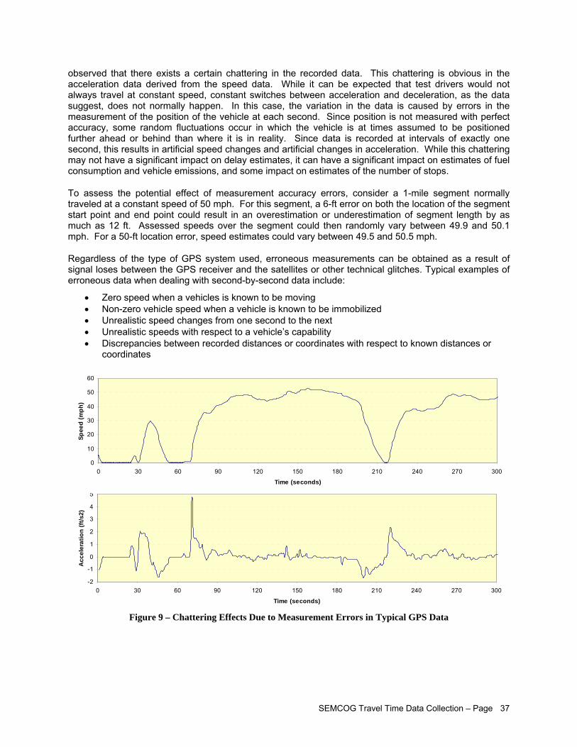
SEMCOG Travel Time Data Collection – Page 37
observed that there exists a certain chattering in the recorded data. This chattering is obvious in the acceleration data derived from the speed data. While it can be expected that test drivers would not always travel at constant speed, constant switches between acceleration and deceleration, as the data suggest, does not normally happen. In this case, the variation in the data is caused by errors in the measurement of the position of the vehicle at each second. Since position is not measured with perfect accuracy, some random fluctuations occur in which the vehicle is at times assumed to be positioned further ahead or behind than where it is in reality. Since data is recorded at intervals of exactly one second, this results in artificial speed changes and artificial changes in acceleration. While this chattering may not have a significant impact on delay estimates, it can have a significant impact on estimates of fuel consumption and vehicle emissions, and some impact on estimates of the number of stops.
To assess the potential effect of measurement accuracy errors, consider a 1-mile segment normally traveled at a constant speed of 50 mph. For this segment, a 6-ft error on both the location of the segment start point and end point could result in an overestimation or underestimation of segment length by as much as 12 ft. Assessed speeds over the segment could then randomly vary between 49.9 and 50.1 mph. For a 50-ft location error, speed estimates could vary between 49.5 and 50.5 mph.
Regardless of the type of GPS system used, erroneous measurements can be obtained as a result of signal loses between the GPS receiver and the satellites or other technical glitches. Typical examples of erroneous data when dealing with second-by-second data include:
• Zero speed when a vehicles is known to be moving • Non-zero vehicle speed when a vehicle is known to be immobilized • Unrealistic speed changes from one second to the next • Unrealistic speeds with respect to a vehicle’s capability • Discrepancies between recorded distances or coordinates with respect to known distances or
coordinates
-2
-1
0
1
2
3
4
5
0 30 60 90 120 150 180 210 240 270 300
Time (seconds)
Acc
eler
atio
n (f
t/s2)
0
10
20
30
40
50
60
0 30 60 90 120 150 180 210 240 270 300
Time (seconds)
Spee
d (m
ph)
Figure 9 – Chattering Effects Due to Measurement Errors in Typical GPS Data
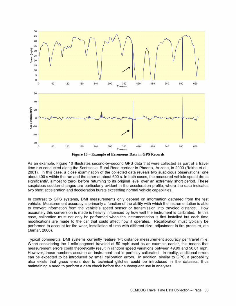
SEMCOG Travel Time Data Collection – Page 38
0
5
10
15
20
25
30
35
40
45
50
0 60 120 180 240 300 360 420 480 540 600 660Time (s)
Spee
d (m
ph)
-60
-40
-20
0
20
40
60
0 60 120 180 240 300 360 420 480 540 600 660Time (s)
Acc
eler
atio
n (f
t/s2 )
Figure 10 – Example of Erroneous Data in GPS Records
As an example, Figure 10 illustrates second-by-second GPS data that were collected as part of a travel time run conducted along the Scottsdale–Rural Road corridor in Phoenix, Arizona, in 2000 (Rakha et al., 2001). In this case, a close examination of the collected data reveals two suspicious observations: one about 400 s within the run and the other at about 600 s. In both cases, the measured vehicle speed drops significantly, almost to zero, before returning to its original level over an extremely short period. These suspicious sudden changes are particularly evident in the acceleration profile, where the data indicates two short acceleration and deceleration bursts exceeding normal vehicle capabilities.
In contrast to GPS systems, DMI measurements only depend on information gathered from the test vehicle. Measurement accuracy is primarily a function of the ability with which the instrumentation is able to convert information from the vehicle’s speed sensor or transmission into traveled distance. How accurately this conversion is made is heavily influenced by how well the instrument is calibrated. In this case, calibration must not only be performed when the instrumentation is first installed but each time modifications are made to the car that could affect how it operates. Recalibration must typically be performed to account for tire wear, installation of tires with different size, adjustment in tire pressure, etc (Jamar, 2006).
Typical commercial DMI systems currently feature 1-ft distance measurement accuracy per travel mile. When considering the 1-mile segment traveled at 50 mph used as an example earlier, this means that measurement errors could theoretically result in random speed variations between 49.99 and 50.01 mph. However, these numbers assume an instrument that is perfectly calibrated. In reality, additional errors can be expected to be introduced by small calibration errors. In addition, similar to GPS, a probability also exists that gross errors due to technical glitches could be introduced in the datasets, thus maintaining a need to perform a data check before their subsequent use in analyses.
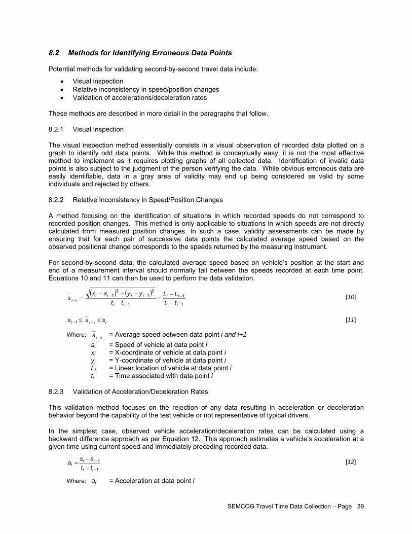
SEMCOG Travel Time Data Collection – Page 39
8.2 Methods for Identifying Erroneous Data Points
Potential methods for validating second-by-second travel data include:
• Visual inspection • Relative inconsistency in speed/position changes • Validation of accelerations/deceleration rates
These methods are described in more detail in the paragraphs that follow.
8.2.1 Visual Inspection
The visual inspection method essentially consists in a visual observation of recorded data plotted on a graph to identify odd data points. While this method is conceptually easy, it is not the most effective method to implement as it requires plotting graphs of all collected data. Identification of invalid data points is also subject to the judgment of the person verifying the data. While obvious erroneous data are easily identifiable, data in a gray area of validity may end up being considered as valid by some individuals and rejected by others.
8.2.2 Relative Inconsistency in Speed/Position Changes
A method focusing on the identification of situations in which recorded speeds do not correspond to recorded position changes. This method is only applicable to situations in which speeds are not directly calculated from measured position changes. In such a case, validity assessments can be made by ensuring that for each pair of successive data points the calculated average speed based on the observed positional change corresponds to the speeds returned by the measuring instrument.
For second-by-second data, the calculated average speed based on vehicle’s position at the start and end of a measurement interval should normally fall between the speeds recorded at each time point. Equations 10 and 11 can then be used to perform the data validation.
( ) ( )1
1
1
21
21
,1−
−
−
−−
−−
=−
−+−=−
ii
ii
ii
iiii
ttLL
ttyyxx
s ii [10]
ii sss ii ,11 ≤≤ −− [11]
Where: iis ,1− = Average speed between data point i and i+1
si = Speed of vehicle at data point i xi = X-coordinate of vehicle at data point i yi = Y-coordinate of vehicle at data point i Li = Linear location of vehicle at data point i ti = Time associated with data point i
8.2.3 Validation of Acceleration/Deceleration Rates
This validation method focuses on the rejection of any data resulting in acceleration or deceleration behavior beyond the capability of the test vehicle or not representative of typical drivers.
In the simplest case, observed vehicle acceleration/deceleration rates can be calculated using a backward difference approach as per Equation 12. This approach estimates a vehicle’s acceleration at a given time using current speed and immediately preceding recorded data.
1
1 −
−
−−
=ii
iii tt
ssa [12]
Where: ai = Acceleration at data point i
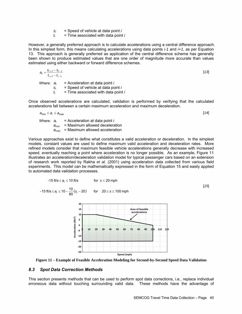
SEMCOG Travel Time Data Collection – Page 40
si = Speed of vehicle at data point i ti = Time associated with data point i
However, a generally preferred approach is to calculate accelerations using a central difference approach. In this simplest form, this means calculating accelerations using data points i-1 and i+1, as per Equation 13. This approach is generally preferred as application of the central difference scheme has generally been shown to produce estimated values that are one order of magnitude more accurate than values estimated using either backward or forward difference schemes.
11
11 −+
−+
−−
=ii
iii tt
ssa [13]
Where: ai = Acceleration at data point i si = Speed of vehicle at data point i ti = Time associated with data point i
Once observed accelerations are calculated, validation is performed by verifying that the calculated accelerations fall between a certain maximum acceleration and maximum deceleration.
maxmin aaa i ≤≤ [14]
Where: ai = Acceleration at data point i amin = Maximum allowed deceleration amax = Maximum allowed acceleration
Various approaches exist to define what constitutes a valid acceleration or deceleration. In the simplest models, constant values are used to define maximum valid acceleration and deceleration rates. More refined models consider that maximum feasible vehicle accelerations generally decrease with increased speed, eventually reaching a point where acceleration is no longer possible. As an example, Figure 11 illustrates an acceleration/deceleration validation model for typical passenger cars based on an extension of research work reported by Rakha et al. (2001) using acceleration data collected from various field experiments. This model can be mathematically expressed in the form of Equation 15 and easily applied to automated data validation processes.
( ) mph 100 20 for 20
801010 ft/s 15-
mph 20 for ft/s 01 ft/s -15
≤≤−−≤≤
≤≤≤
ssa
sa
ii
i
[15]
-25
-20
-15
-10
-5
0
5
10
15
20
0 10 20 30 40 50 60 70 80 90 100 110 120
Speed (mph)
Acc
eler
atio
n (ft
/s2 )
Area of feasible accelerations
Figure 11 – Example of Feasible Acceleration Modeling for Second-by-Second Speed Data Validation
8.3 Spot Data Correction Methods
This section presents methods that can be used to perform spot data corrections, i.e., replace individual erroneous data without touching surrounding valid data. These methods have the advantage of
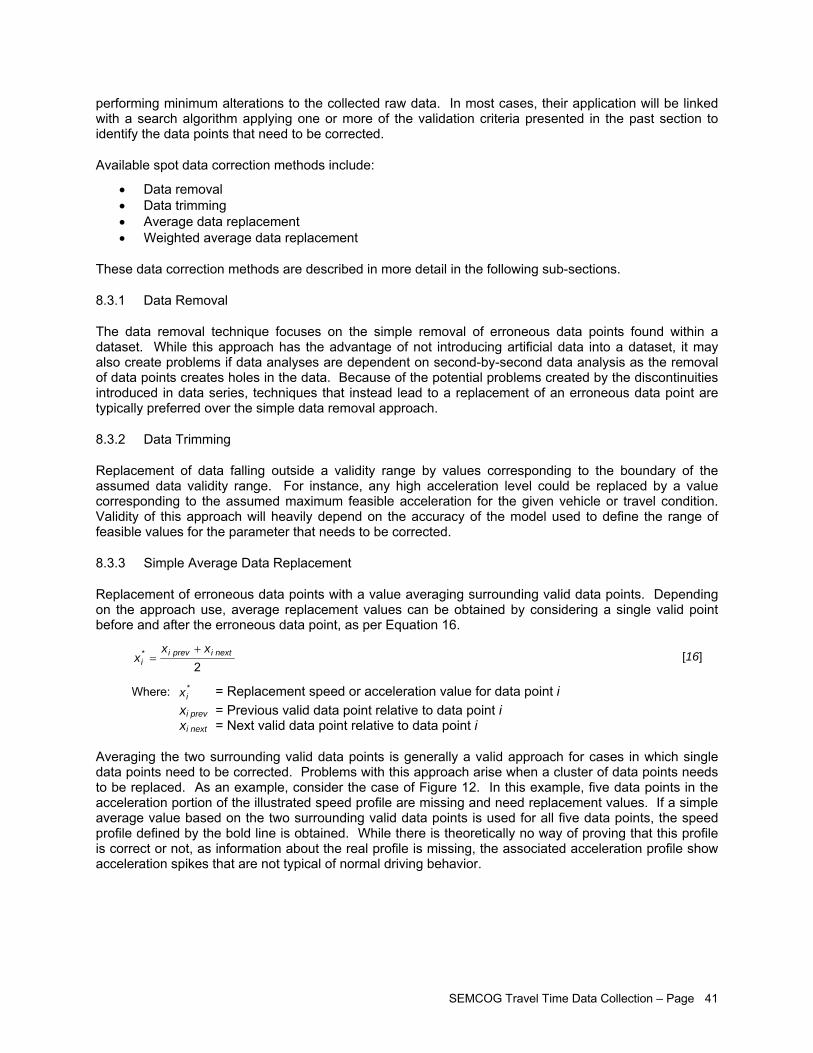
SEMCOG Travel Time Data Collection – Page 41
performing minimum alterations to the collected raw data. In most cases, their application will be linked with a search algorithm applying one or more of the validation criteria presented in the past section to identify the data points that need to be corrected.
Available spot data correction methods include:
• Data removal • Data trimming • Average data replacement • Weighted average data replacement
These data correction methods are described in more detail in the following sub-sections.
8.3.1 Data Removal
The data removal technique focuses on the simple removal of erroneous data points found within a dataset. While this approach has the advantage of not introducing artificial data into a dataset, it may also create problems if data analyses are dependent on second-by-second data analysis as the removal of data points creates holes in the data. Because of the potential problems created by the discontinuities introduced in data series, techniques that instead lead to a replacement of an erroneous data point are typically preferred over the simple data removal approach.
8.3.2 Data Trimming
Replacement of data falling outside a validity range by values corresponding to the boundary of the assumed data validity range. For instance, any high acceleration level could be replaced by a value corresponding to the assumed maximum feasible acceleration for the given vehicle or travel condition. Validity of this approach will heavily depend on the accuracy of the model used to define the range of feasible values for the parameter that needs to be corrected.
8.3.3 Simple Average Data Replacement
Replacement of erroneous data points with a value averaging surrounding valid data points. Depending on the approach use, average replacement values can be obtained by considering a single valid point before and after the erroneous data point, as per Equation 16.
2 * nextiprevi
ixx
x+
= [16]
Where: *ix = Replacement speed or acceleration value for data point i
xi prev = Previous valid data point relative to data point i xi next = Next valid data point relative to data point i
Averaging the two surrounding valid data points is generally a valid approach for cases in which single data points need to be corrected. Problems with this approach arise when a cluster of data points needs to be replaced. As an example, consider the case of Figure 12. In this example, five data points in the acceleration portion of the illustrated speed profile are missing and need replacement values. If a simple average value based on the two surrounding valid data points is used for all five data points, the speed profile defined by the bold line is obtained. While there is theoretically no way of proving that this profile is correct or not, as information about the real profile is missing, the associated acceleration profile show acceleration spikes that are not typical of normal driving behavior.
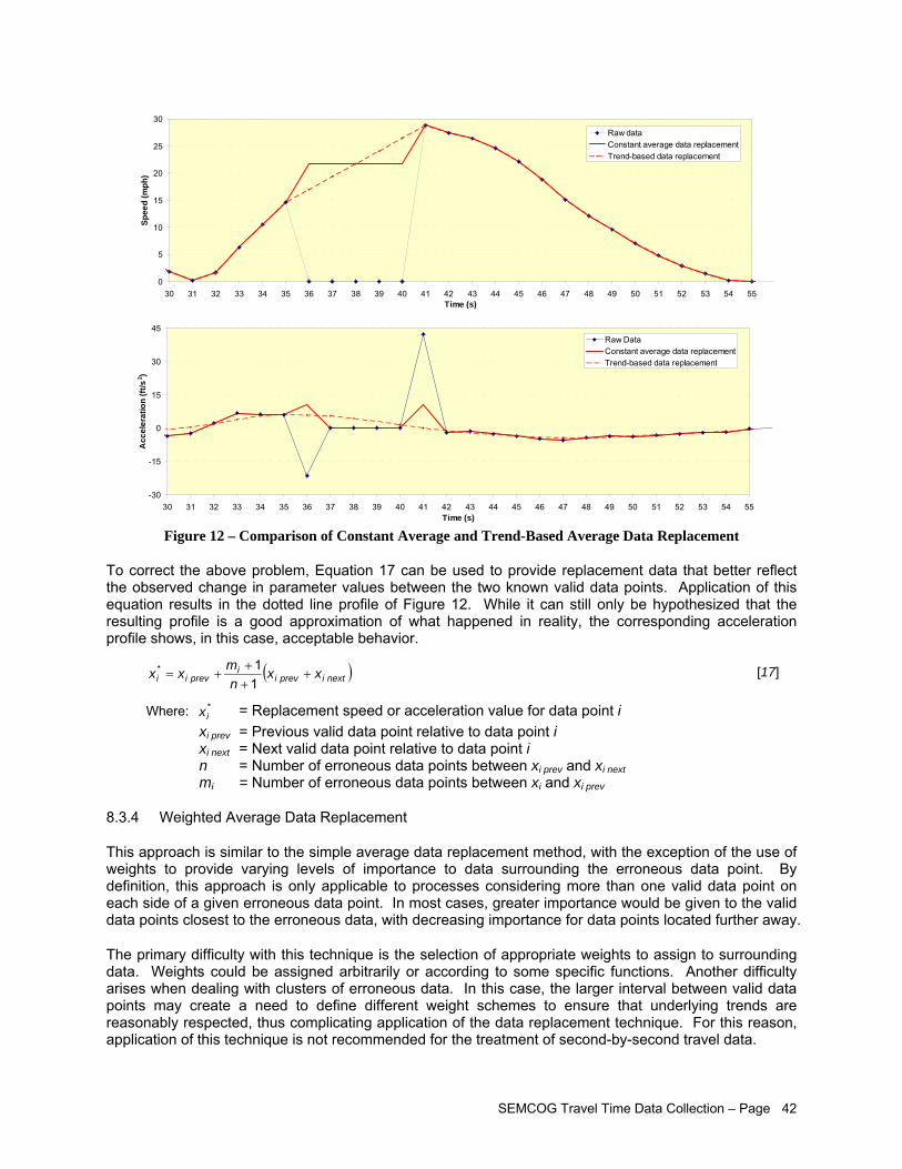
SEMCOG Travel Time Data Collection – Page 42
0
5
10
15
20
25
30
30 31 32 33 34 35 36 37 38 39 40 41 42 43 44 45 46 47 48 49 50 51 52 53 54 55Time (s)
Spee
d (m
ph)
Raw dataConstant average data replacementTrend-based data replacement
-30
-15
0
15
30
45
30 31 32 33 34 35 36 37 38 39 40 41 42 43 44 45 46 47 48 49 50 51 52 53 54 55Time (s)
Acc
eler
atio
n (ft
/s2 )
Raw DataConstant average data replacementTrend-based data replacement
Figure 12 – Comparison of Constant Average and Trend-Based Average Data Replacement
To correct the above problem, Equation 17 can be used to provide replacement data that better reflect the observed change in parameter values between the two known valid data points. Application of this equation results in the dotted line profile of Figure 12. While it can still only be hypothesized that the resulting profile is a good approximation of what happened in reality, the corresponding acceleration profile shows, in this case, acceptable behavior.
( )nextiprevii
previi xxn
mxx *
11
+++
+= [17]
Where: *ix = Replacement speed or acceleration value for data point i
xi prev = Previous valid data point relative to data point i xi next = Next valid data point relative to data point i n = Number of erroneous data points between xi prev and xi next
mi = Number of erroneous data points between xi and xi prev
8.3.4 Weighted Average Data Replacement
This approach is similar to the simple average data replacement method, with the exception of the use of weights to provide varying levels of importance to data surrounding the erroneous data point. By definition, this approach is only applicable to processes considering more than one valid data point on each side of a given erroneous data point. In most cases, greater importance would be given to the valid data points closest to the erroneous data, with decreasing importance for data points located further away.
The primary difficulty with this technique is the selection of appropriate weights to assign to surrounding data. Weights could be assigned arbitrarily or according to some specific functions. Another difficulty arises when dealing with clusters of erroneous data. In this case, the larger interval between valid data points may create a need to define different weight schemes to ensure that underlying trends are reasonably respected, thus complicating application of the data replacement technique. For this reason, application of this technique is not recommended for the treatment of second-by-second travel data.
SEMCOG Travel Time Data Collection – Page 43
8.4 Data Smoothing Techniques
Data smoothing techniques are used to eliminate noise in data series and extract real trends and patterns. As explained previously, measurement errors could result in slight variations in recorded data from one interval to the next. This effect is illustrated in Figure 13 using speed and acceleration data collected along US-24 in May 2007 with a GPS-equipped test vehicle. In this case, while recorded speeds appear to increase or decrease smoothly over the illustrated interval, small random fluctuations can be noticed when looking at the data on a second-by-second basis. These small fluctuations are particularly evident when analyzing the acceleration data that can be derived from the speed data.
0
10
20
30
40
50
60
30 45 60 75 90 105 120 135 150 165 180 195 210 225 240Time (s)
Spee
d (m
ph)
-10
-5
0
5
10
15
20
30 45 60 75 90 105 120 135 150 165 180 195 210 225 240Time (s)
Acc
eler
atio
n (f
t/s2 )
Figure 13 – Measurement Noise for Data Recorded on US-24 near Detroit, Michigan in May 2007
Random fluctuations in recorded speeds are not likely to have significant effects on travel time, average speed or delay estimates. However, these fluctuations can have a significant impact on estimates of fuel consumption and vehicle emission. This is because assessment of these parameters is typically linked to an analysis of speed fluctuations from one interval to the next. Estimates of the number of stops associated with a particular trip could also be affected if the number of stops is derived by compiling speed changes from one interval to the next. However, impact on the assessed number of stops is generally expected to be relatively small when compared to the potential impact on fuel consumption and emission parameters.
While various smoothing techniques are described in the literature, not all techniques are available for processing second-by-second trip data. First, as evidenced in Figures 9 and 10, trip data do not necessarily exhibit cyclic patterns or follow long-term uniform trends. This means that techniques primarily designed to identify patterns or trends must not be considered. Among the remaining potential candidates techniques are:
• Simple moving average • Simple exponential smoothing • Kernel smoothing
These techniques are described in more detail below.
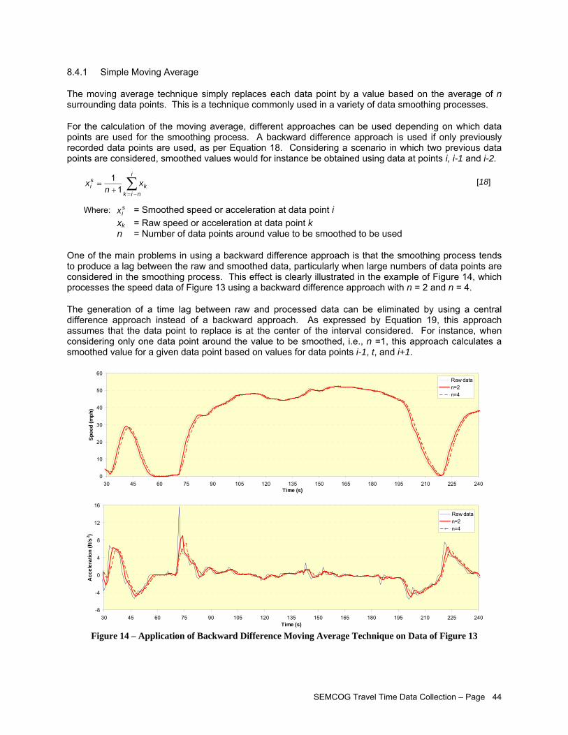
SEMCOG Travel Time Data Collection – Page 44
8.4.1 Simple Moving Average
The moving average technique simply replaces each data point by a value based on the average of n surrounding data points. This is a technique commonly used in a variety of data smoothing processes.
For the calculation of the moving average, different approaches can be used depending on which data points are used for the smoothing process. A backward difference approach is used if only previously recorded data points are used, as per Equation 18. Considering a scenario in which two previous data points are considered, smoothed values would for instance be obtained using data at points i, i-1 and i-2.
∑−=+
=i
nikk
si x
nx
11 [18]
Where: six = Smoothed speed or acceleration at data point i
xk = Raw speed or acceleration at data point k n = Number of data points around value to be smoothed to be used
One of the main problems in using a backward difference approach is that the smoothing process tends to produce a lag between the raw and smoothed data, particularly when large numbers of data points are considered in the smoothing process. This effect is clearly illustrated in the example of Figure 14, which processes the speed data of Figure 13 using a backward difference approach with n = 2 and n = 4.
The generation of a time lag between raw and processed data can be eliminated by using a central difference approach instead of a backward approach. As expressed by Equation 19, this approach assumes that the data point to replace is at the center of the interval considered. For instance, when considering only one data point around the value to be smoothed, i.e., n =1, this approach calculates a smoothed value for a given data point based on values for data points i-1, t, and i+1.
0
10
20
30
40
50
60
30 45 60 75 90 105 120 135 150 165 180 195 210 225 240Time (s)
Spee
d (m
ph)
Raw datan=2n=4
-8
-4
0
4
8
12
16
30 45 60 75 90 105 120 135 150 165 180 195 210 225 240Time (s)
Acc
eler
atio
n (ft
/s2 )
Raw datan=2n=4
Figure 14 – Application of Backward Difference Moving Average Technique on Data of Figure 13
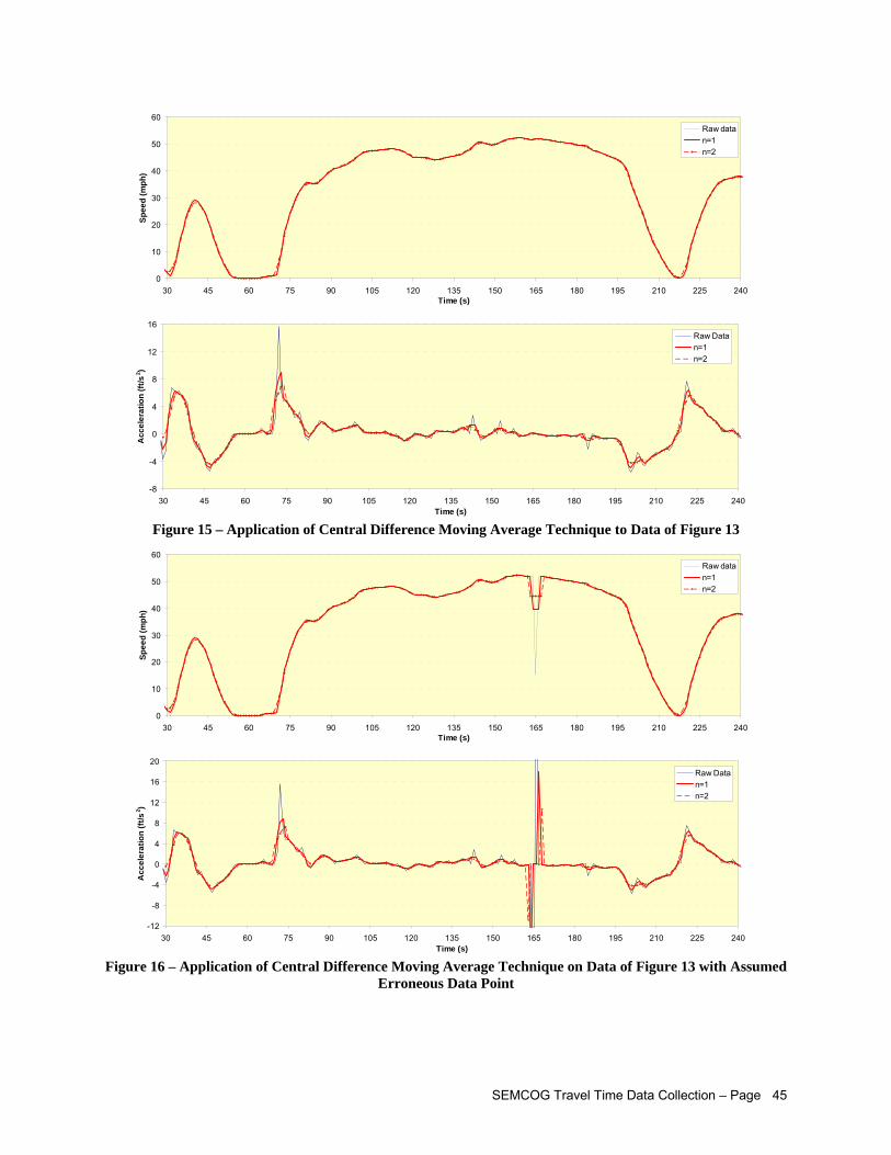
SEMCOG Travel Time Data Collection – Page 45
0
10
20
30
40
50
60
30 45 60 75 90 105 120 135 150 165 180 195 210 225 240Time (s)
Spee
d (m
ph)
Raw datan=1n=2
-8
-4
0
4
8
12
16
30 45 60 75 90 105 120 135 150 165 180 195 210 225 240Time (s)
Acc
eler
atio
n (ft
/s2 )
Raw Datan=1n=2
Figure 15 – Application of Central Difference Moving Average Technique to Data of Figure 13
0
10
20
30
40
50
60
30 45 60 75 90 105 120 135 150 165 180 195 210 225 240Time (s)
Spee
d (m
ph)
Raw datan=1n=2
-12
-8
-4
0
4
8
12
16
20
30 45 60 75 90 105 120 135 150 165 180 195 210 225 240Time (s)
Acc
eler
atio
n (ft
/s2 )
Raw Datan=1n=2
Figure 16 – Application of Central Difference Moving Average Technique on Data of Figure 13 with Assumed
Erroneous Data Point
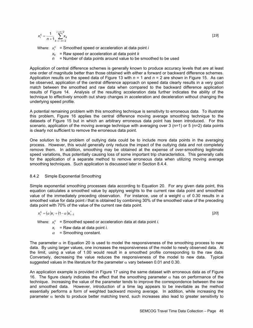
SEMCOG Travel Time Data Collection – Page 46
∑+
−=+=
2/
2/11 ni
nikk
si x
nx [19]
Where: six = Smoothed speed or acceleration at data point i
xk = Raw speed or acceleration at data point k n = Number of data points around value to be smoothed to be used
Application of central difference schemes is generally known to produce accuracy levels that are at least one order of magnitude better than those obtained with either a forward or backward difference schemes. Application results on the speed data of Figure 13 with n = 1 and n = 2 are shown in Figure 15. As can be observed, application of the central difference approach on speed data clearly results in a very good match between the smoothed and raw data when compared to the backward difference application results of Figure 14. Analysis of the resulting acceleration data further indicates the ability of the technique to effectively smooth out sharp changes in acceleration and deceleration without changing the underlying speed profile.
A potential remaining problem with this smoothing technique is sensitivity to erroneous data. To illustrate this problem, Figure 16 applies the central difference moving average smoothing technique to the datasets of Figure 15 but in which an arbitrary erroneous data point has been introduced. For this scenario, application of the moving average technique with averaging over 3 (n=1) or 5 (n=2) data points is clearly not sufficient to remove the erroneous data point.
One solution to the problem of outlying data could be to include more data points in the averaging process. However, this would generally only reduce the impact of the outlying data and not completely remove them. In addition, smoothing may be obtained at the expense of over-smoothing legitimate speed variations, thus potentially causing loss of some important trip characteristics. This generally calls for the application of a separate method to remove erroneous data when utilizing moving average smoothing techniques. Such application is discussed later in Section 8.4.4.
8.4.2 Simple Exponential Smoothing
Simple exponential smoothing processes data according to Equation 20. For any given data point, this equation calculates a smoothed value by applying weights to the current raw data point and smoothed value of the immediately preceding observation. For instance, use of a weight α of 0.30 results in a smoothed value for data point i that is obtained by combining 30% of the smoothed value of the preceding data point with 70% of the value of the current raw data point.
( ) ( ) *11 −−+= ii
si xxx αα [20]
Where: six = Smoothed speed or acceleration data at data point i.
xi = Raw data at data point i. α = Smoothing constant.
The parameter α in Equation 20 is used to model the responsiveness of the smoothing process to new data. By using larger values, one increases the responsiveness of the model to newly observed data. At the limit, using a value of 1.00 would result in a smoothed profile corresponding to the raw data. Conversely, decreasing the value reduces the responsiveness of the model to new data. Typical suggested values in the literature for the parameter α vary between 0.01 and 0.30.
An application example is provided in Figure 17 using the same dataset with erroneous data as of Figure 16. The figure clearly indicates the effect that the smoothing parameter α has on performance of the technique. Increasing the value of the parameter tends to improve the correspondence between the raw and smoothed data. However, introduction of a time lag appears to be inevitable as the method essentially performs a form of weighted backward moving average. In addition, while increasing the parameter α tends to produce better matching trend, such increases also lead to greater sensitivity to
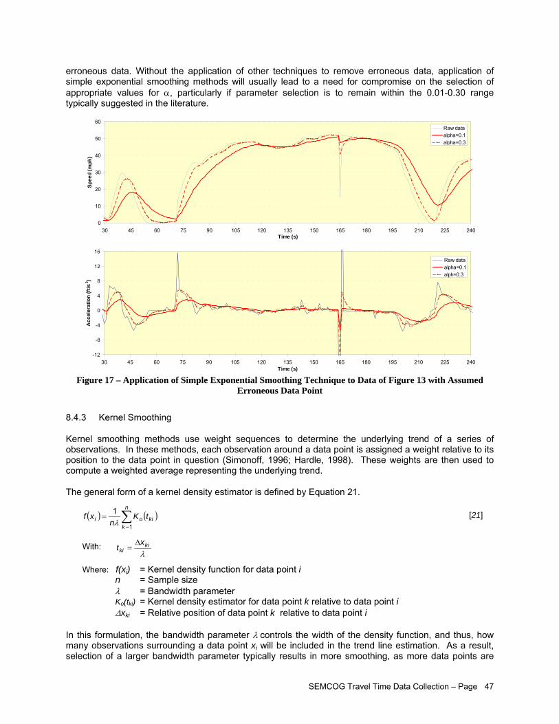
SEMCOG Travel Time Data Collection – Page 47
erroneous data. Without the application of other techniques to remove erroneous data, application of simple exponential smoothing methods will usually lead to a need for compromise on the selection of appropriate values for α, particularly if parameter selection is to remain within the 0.01-0.30 range typically suggested in the literature.
0
10
20
30
40
50
60
30 45 60 75 90 105 120 135 150 165 180 195 210 225 240Time (s)
Spee
d (m
ph)
Raw dataalpha=0.1alpha=0.3
-12
-8
-4
0
4
8
12
16
30 45 60 75 90 105 120 135 150 165 180 195 210 225 240Time (s)
Acc
eler
atio
n (ft
/s2 )
Raw dataalpha=0.1alph=0.3
Figure 17 – Application of Simple Exponential Smoothing Technique to Data of Figure 13 with Assumed
Erroneous Data Point
8.4.3 Kernel Smoothing
Kernel smoothing methods use weight sequences to determine the underlying trend of a series of observations. In these methods, each observation around a data point is assigned a weight relative to its position to the data point in question (Simonoff, 1996; Hardle, 1998). These weights are then used to compute a weighted average representing the underlying trend.
The general form of a kernel density estimator is defined by Equation 21.
( ) ( )∑=
=n
kkioi tK
nxf
1
1λ
[21]
With: λ
kiki
xt ∆=
Where: f(xi) = Kernel density function for data point i n = Sample size λ = Bandwidth parameter Ko(tki) = Kernel density estimator for data point k relative to data point i ∆xki = Relative position of data point k relative to data point i
In this formulation, the bandwidth parameter λ controls the width of the density function, and thus, how many observations surrounding a data point xi will be included in the trend line estimation. As a result, selection of a larger bandwidth parameter typically results in more smoothing, as more data points are
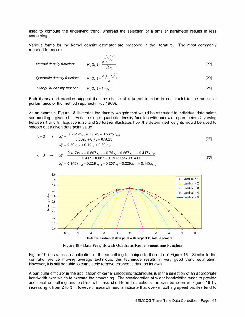
SEMCOG Travel Time Data Collection – Page 48
used to compute the underlying trend, whereas the selection of a smaller parameter results in less smoothing.
Various forms for the kernel density estimator are proposed in the literature. The most commonly reported forms are:
Normal density function: π2
)(2
2
⎟⎟⎠
⎞⎜⎜⎝
⎛−
=
kit
kioetK [22]
Quadratic density function: ( )4
1 3)(2
kikio
ttK −= [23]
Triangular density function: kikio ttK −= 1)( [24]
Both theory and practice suggest that the choice of a kernel function is not crucial to the statistical performance of the method (Epanechnikov 1969).
As an example, Figure 18 illustrates the density weights that would be attributed to individual data points surrounding a given observation using a quadratic density function with bandwidth parameters λ varying between 1 and 5. Equations 25 and 26 further illustrates how the determined weights would be used to smooth out a given data point value
11
11
30.040.030.0 5625.075.05625.05625.075.05625.0 2
+−
+−
++=++++
=→=
iiisi
iiisi
xxxx
xxxxλ [25]
2112
2112
143.0229.0257.0229.0143.0 417.0667.075.0667.0417.0
417.0667.075.0667.0417.0 3
++−−
++−−
++++=++++
++++=→=
iiiiisi
iiiiisi
xxxxxx
xxxxxxλ [26]
0.0
0.1
0.2
0.3
0.4
0.5
0.6
0.7
0.8
0.9
1.0
-5 -4 -3 -2 -1 0 1 2 3 4 5
Relative position of data point with respect to data to smooth
Dens
ity v
alue
Lambda = 1Lambda = 2Lambda = 3Lambda = 4Lambda = 5
Figure 18 – Data Weights with Quadratic Kernel Smoothing Function
Figure 19 illustrates an application of the smoothing technique to the data of Figure 16. Similar to the central-difference moving average technique, this technique results in very good trend estimation. However, it is still not able to completely remove erroneous data on its own.
A particular difficulty in the application of kernel smoothing techniques is in the selection of an appropriate bandwidth over which to execute the smoothing. The consideration of wider bandwidths tends to provide additional smoothing and profiles with less short-term fluctuations, as can be seen in Figure 19 by increasing λ from 2 to 3. However, research results indicate that over-smoothing speed profiles tend to
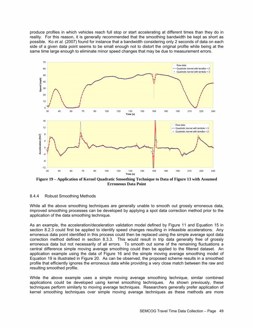
SEMCOG Travel Time Data Collection – Page 49
produce profiles in which vehicles reach full stop or start accelerating at different times than they do in reality. For this reason, it is generally recommended that the smoothing bandwidth be kept as short as possible. Ko et al. (2007) found for instance that a bandwidth considering only 2 seconds of data on each side of a given data point seems to be small enough not to distort the original profile while being at the same time large enough to eliminate minor speed changes that may be due to measurement errors.
0
10
20
30
40
50
60
70
30 45 60 75 90 105 120 135 150 165 180 195 210 225 240Time (s)
Spee
d (m
ph)
Raw dataQuadratic kernel with lamdba = 2Quadratic kernel with lambda = 3
-12
-8
-4
0
4
8
12
16
30 45 60 75 90 105 120 135 150 165 180 195 210 225 240Time (s)
Acc
eler
atio
n (f
t/s2 )
Raw dataQuadratic kernel with lambda = 3Quadratic kernel with lamdba = 2
Figure 19 – Application of Kernel Quadratic Smoothing Technique to Data of Figure 13 with Assumed
Erroneous Data Point
8.4.4 Robust Smoothing Methods
While all the above smoothing techniques are generally unable to smooth out grossly erroneous data, improved smoothing processes can be developed by applying a spot data correction method prior to the application of the data smoothing technique.
As an example, the acceleration/deceleration validation model defined by Figure 11 and Equation 15 in section 8.2.3 could first be applied to identify speed changes resulting in infeasible accelerations. Any erroneous data point identified in this process could then be replaced using the simple average spot data correction method defined in section 8.3.3. This would result in trip data generally free of grossly erroneous data but not necessarily of all errors. To smooth out some of the remaining fluctuations a central difference simple moving average smoothing could then be applied to the filtered dataset. An application example using the data of Figure 16 and the simple moving average smoothing model of Equation 19 is illustrated in Figure 20. As can be observed, the proposed scheme results in a smoothed profile that efficiently ignores the erroneous data while providing a very close match between the raw and resulting smoothed profile.
While the above example uses a simple moving average smoothing technique, similar combined applications could be developed using kernel smoothing techniques. As shown previously, these techniques perform similarly to moving average techniques. Researchers generally prefer application of kernel smoothing techniques over simple moving average techniques as these methods are more
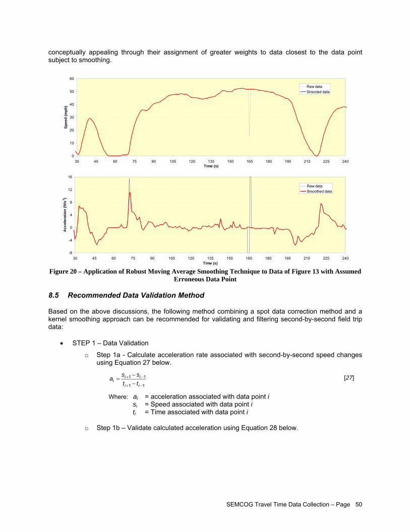
SEMCOG Travel Time Data Collection – Page 50
conceptually appealing through their assignment of greater weights to data closest to the data point subject to smoothing.
0
10
20
30
40
50
60
30 45 60 75 90 105 120 135 150 165 180 195 210 225 240Time (s)
Spee
d (m
ph)
Raw dataSmooted data
-8
-4
0
4
8
12
16
30 45 60 75 90 105 120 135 150 165 180 195 210 225 240Time (s)
Acc
eler
atio
n (ft
/s2 )
Raw dataSmoothed data
Figure 20 – Application of Robust Moving Average Smoothing Technique to Data of Figure 13 with Assumed
Erroneous Data Point
8.5 Recommended Data Validation Method
Based on the above discussions, the following method combining a spot data correction method and a kernel smoothing approach can be recommended for validating and filtering second-by-second field trip data:
• STEP 1 – Data Validation
o Step 1a - Calculate acceleration rate associated with second-by-second speed changes using Equation 27 below.
11
11 −+
−+
−−
=ii
iii tt
ssa [27]
Where: ai = acceleration associated with data point i si = Speed associated with data point i
ti = Time associated with data point i
o Step 1b – Validate calculated acceleration using Equation 28 below.
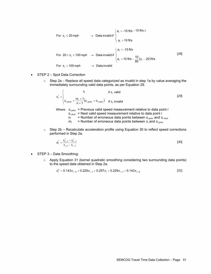
SEMCOG Travel Time Data Collection – Page 51
( )
invalid Data mph 100 For
ft/s 208010ft/s 10
ft/s -15
if invalid Data mph 100 20 For
ft/s 15-
ft/s 01
ft/s -15 if invalid Data mph 20 For
→>
⎪⎩
⎪⎨
⎧
−−>
<
→≤≤
≤
⎪⎩
⎪⎨
⎧
>
<→≤
i
ii
i
i
i
i
i
s
sa
a
s
a
as
[28]
• STEP 2 – Spot Data Correction
o Step 2a – Replace all speed data categorized as invalid in step 1a by value averaging the immediately surrounding valid data points, as per Equation 29.
( ) invalid if
valid if
11
*
i
i
nextiprevii
previ
i
i
s
s
ssn
ms
s
s⎪⎩
⎪⎨
⎧
+++
+= [29]
Where: si prev = Previous valid speed measurement relative to data point i si next = Next valid speed measurement relative to data point i
ni = Number of erroneous data points between si prev and si next mi = Number of erroneous data points between si and si prev
o Step 2b – Recalculate acceleration profile using Equation 30 to reflect speed corrections performed in Step 2a.
11
*1
*1*
−+
−+
−−
=ii
iii tt
ssa [30]
• STEP 3 – Data Smoothing:
o Apply Equation 31 (kernel quadratic smoothing considering two surrounding data points) to the speed data obtained in Step 2a.
2112 143.0229.0257.0229.0143.0 ++−− ++++= iiiiisi xxxxxs [31]

SEMCOG Travel Time Data Collection – Page 52
9 Data Storage Issues Appropriate data archiving is as important as data collection and validation. It is often very expensive to collect data. To ensure that the collected information will have a life that extends beyond the end of the travel time studies, care should be exercised to properly store data.
A particular element that often limits the future usability of collected data is the storage of raw data without any information allowing the identification of erroneous data points that may have resulted from events that occurred at the time of the data collection. If no mention is made of events affecting data collection beyond what was normally expected, it is likely that such information will be lost over time. In such a case, the danger is that someone else will later use the data assuming that all recorded data represents normal conditions and is valid. If this is not the case, assessments made from the data will be biased and invalid. For instance, knowing that slightly longer than average travel times recorded during a specific weekday may be the result of a short period of a particularly violent thunderstorm may be obvious at the time of the data collection but may be lost over time. If the same data is then used assuming normal weather conditions, longer than normal travel time estimates would then be made based on the available data.
One of the most common mistakes made when storing collected data is to simply put the data on a computer disk somewhere with no appropriate notation. At a minimum, a text file should be included on the disk documenting how the data was collected and processed. The information contained in this file should include:
• Details about surveyed segments • Data collection periods • Weather conditions at time of the data collection • Information about how the travel runs were executed, in particular what factors were used to
terminate or invalidate runs as this affects the type of data collected • Identification of database fields if such identification is not obvious • Whether the stored data are raw or processed data • Methods used for validating and processing data • Explanation of any acronyms used • Names of persons involved in the data collection and data validation
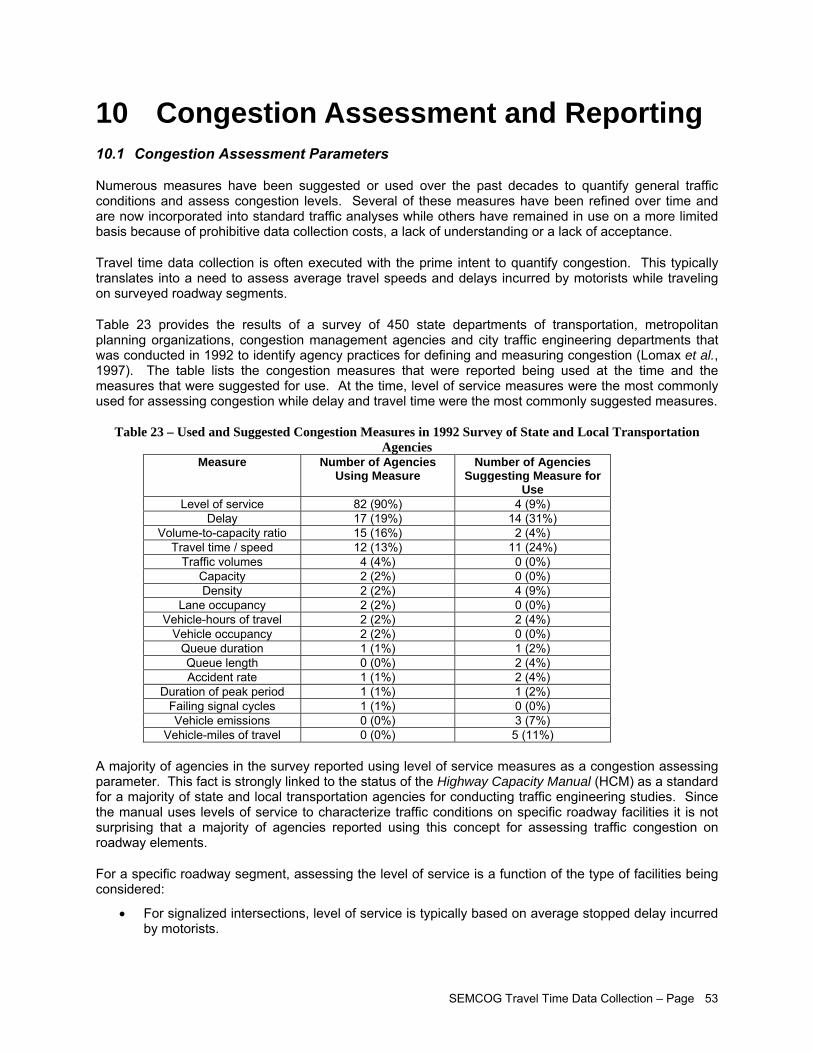
SEMCOG Travel Time Data Collection – Page 53
10 Congestion Assessment and Reporting 10.1 Congestion Assessment Parameters
Numerous measures have been suggested or used over the past decades to quantify general traffic conditions and assess congestion levels. Several of these measures have been refined over time and are now incorporated into standard traffic analyses while others have remained in use on a more limited basis because of prohibitive data collection costs, a lack of understanding or a lack of acceptance.
Travel time data collection is often executed with the prime intent to quantify congestion. This typically translates into a need to assess average travel speeds and delays incurred by motorists while traveling on surveyed roadway segments.
Table 23 provides the results of a survey of 450 state departments of transportation, metropolitan planning organizations, congestion management agencies and city traffic engineering departments that was conducted in 1992 to identify agency practices for defining and measuring congestion (Lomax et al., 1997). The table lists the congestion measures that were reported being used at the time and the measures that were suggested for use. At the time, level of service measures were the most commonly used for assessing congestion while delay and travel time were the most commonly suggested measures.
Table 23 – Used and Suggested Congestion Measures in 1992 Survey of State and Local Transportation Agencies
Measure Number of Agencies Using Measure
Number of Agencies Suggesting Measure for
Use Level of service 82 (90%) 4 (9%)
Delay 17 (19%) 14 (31%) Volume-to-capacity ratio 15 (16%) 2 (4%)
Travel time / speed 12 (13%) 11 (24%) Traffic volumes 4 (4%) 0 (0%)
Capacity 2 (2%) 0 (0%) Density 2 (2%) 4 (9%)
Lane occupancy 2 (2%) 0 (0%) Vehicle-hours of travel 2 (2%) 2 (4%)
Vehicle occupancy 2 (2%) 0 (0%) Queue duration 1 (1%) 1 (2%) Queue length 0 (0%) 2 (4%) Accident rate 1 (1%) 2 (4%)
Duration of peak period 1 (1%) 1 (2%) Failing signal cycles 1 (1%) 0 (0%) Vehicle emissions 0 (0%) 3 (7%)
Vehicle-miles of travel 0 (0%) 5 (11%)
A majority of agencies in the survey reported using level of service measures as a congestion assessing parameter. This fact is strongly linked to the status of the Highway Capacity Manual (HCM) as a standard for a majority of state and local transportation agencies for conducting traffic engineering studies. Since the manual uses levels of service to characterize traffic conditions on specific roadway facilities it is not surprising that a majority of agencies reported using this concept for assessing traffic congestion on roadway elements.
For a specific roadway segment, assessing the level of service is a function of the type of facilities being considered:
• For signalized intersections, level of service is typically based on average stopped delay incurred by motorists.
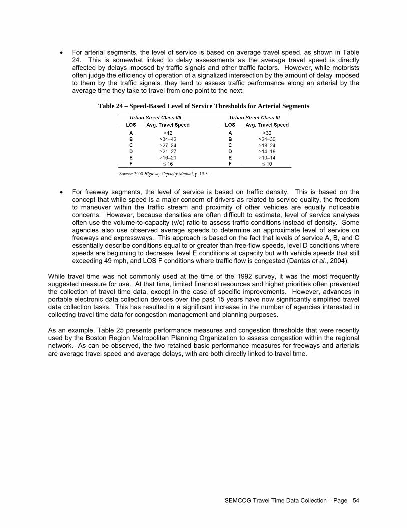
SEMCOG Travel Time Data Collection – Page 54
• For arterial segments, the level of service is based on average travel speed, as shown in Table 24. This is somewhat linked to delay assessments as the average travel speed is directly affected by delays imposed by traffic signals and other traffic factors. However, while motorists often judge the efficiency of operation of a signalized intersection by the amount of delay imposed to them by the traffic signals, they tend to assess traffic performance along an arterial by the average time they take to travel from one point to the next.
Table 24 – Speed-Based Level of Service Thresholds for Arterial Segments
• For freeway segments, the level of service is based on traffic density. This is based on the concept that while speed is a major concern of drivers as related to service quality, the freedom to maneuver within the traffic stream and proximity of other vehicles are equally noticeable concerns. However, because densities are often difficult to estimate, level of service analyses often use the volume-to-capacity (v/c) ratio to assess traffic conditions instead of density. Some agencies also use observed average speeds to determine an approximate level of service on freeways and expressways. This approach is based on the fact that levels of service A, B, and C essentially describe conditions equal to or greater than free-flow speeds, level D conditions where speeds are beginning to decrease, level E conditions at capacity but with vehicle speeds that still exceeding 49 mph, and LOS F conditions where traffic flow is congested (Dantas et al., 2004).
While travel time was not commonly used at the time of the 1992 survey, it was the most frequently suggested measure for use. At that time, limited financial resources and higher priorities often prevented the collection of travel time data, except in the case of specific improvements. However, advances in portable electronic data collection devices over the past 15 years have now significantly simplified travel data collection tasks. This has resulted in a significant increase in the number of agencies interested in collecting travel time data for congestion management and planning purposes.
As an example, Table 25 presents performance measures and congestion thresholds that were recently used by the Boston Region Metropolitan Planning Organization to assess congestion within the regional network. As can be observed, the two retained basic performance measures for freeways and arterials are average travel speed and average delays, with are both directly linked to travel time.
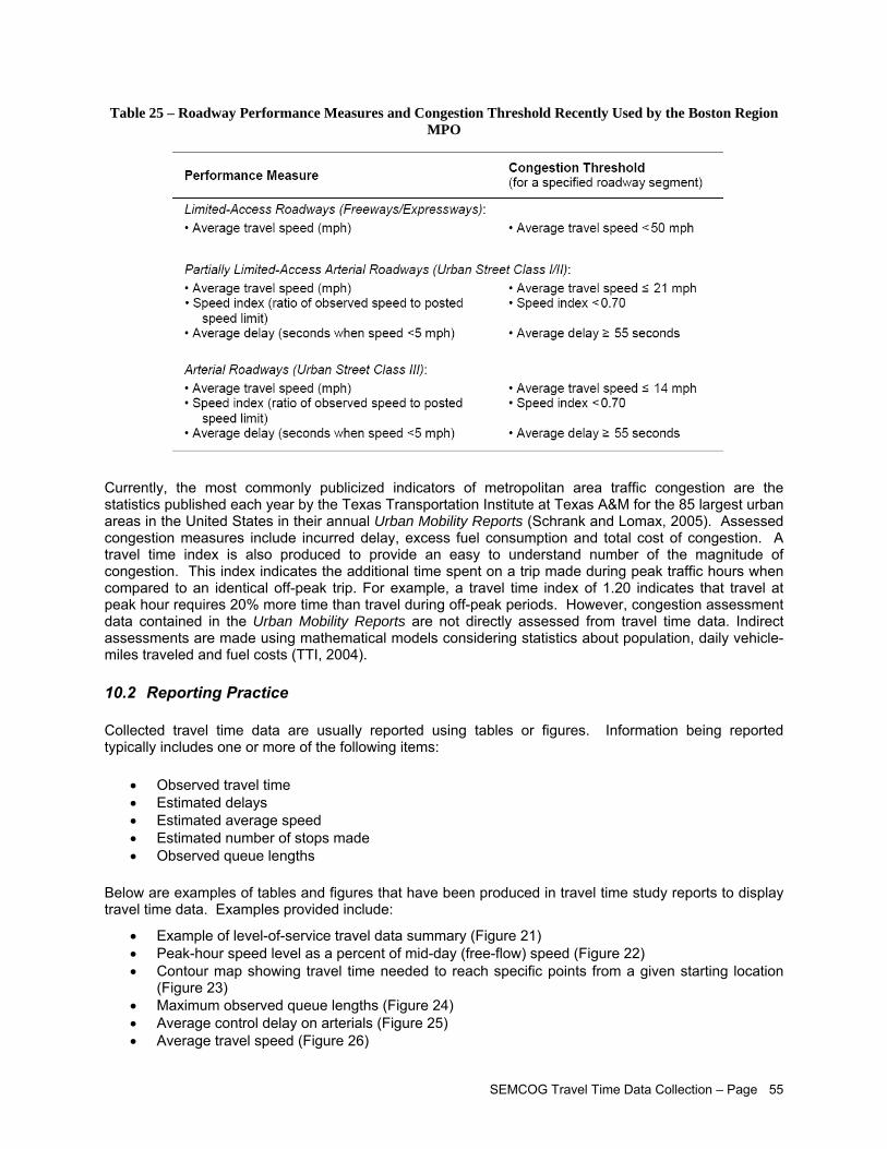
SEMCOG Travel Time Data Collection – Page 55
Table 25 – Roadway Performance Measures and Congestion Threshold Recently Used by the Boston Region MPO
Currently, the most commonly publicized indicators of metropolitan area traffic congestion are the statistics published each year by the Texas Transportation Institute at Texas A&M for the 85 largest urban areas in the United States in their annual Urban Mobility Reports (Schrank and Lomax, 2005). Assessed congestion measures include incurred delay, excess fuel consumption and total cost of congestion. A travel time index is also produced to provide an easy to understand number of the magnitude of congestion. This index indicates the additional time spent on a trip made during peak traffic hours when compared to an identical off-peak trip. For example, a travel time index of 1.20 indicates that travel at peak hour requires 20% more time than travel during off-peak periods. However, congestion assessment data contained in the Urban Mobility Reports are not directly assessed from travel time data. Indirect assessments are made using mathematical models considering statistics about population, daily vehicle-miles traveled and fuel costs (TTI, 2004).
10.2 Reporting Practice
Collected travel time data are usually reported using tables or figures. Information being reported typically includes one or more of the following items:
• Observed travel time • Estimated delays • Estimated average speed • Estimated number of stops made • Observed queue lengths
Below are examples of tables and figures that have been produced in travel time study reports to display travel time data. Examples provided include:
• Example of level-of-service travel data summary (Figure 21) • Peak-hour speed level as a percent of mid-day (free-flow) speed (Figure 22) • Contour map showing travel time needed to reach specific points from a given starting location
(Figure 23) • Maximum observed queue lengths (Figure 24) • Average control delay on arterials (Figure 25) • Average travel speed (Figure 26)
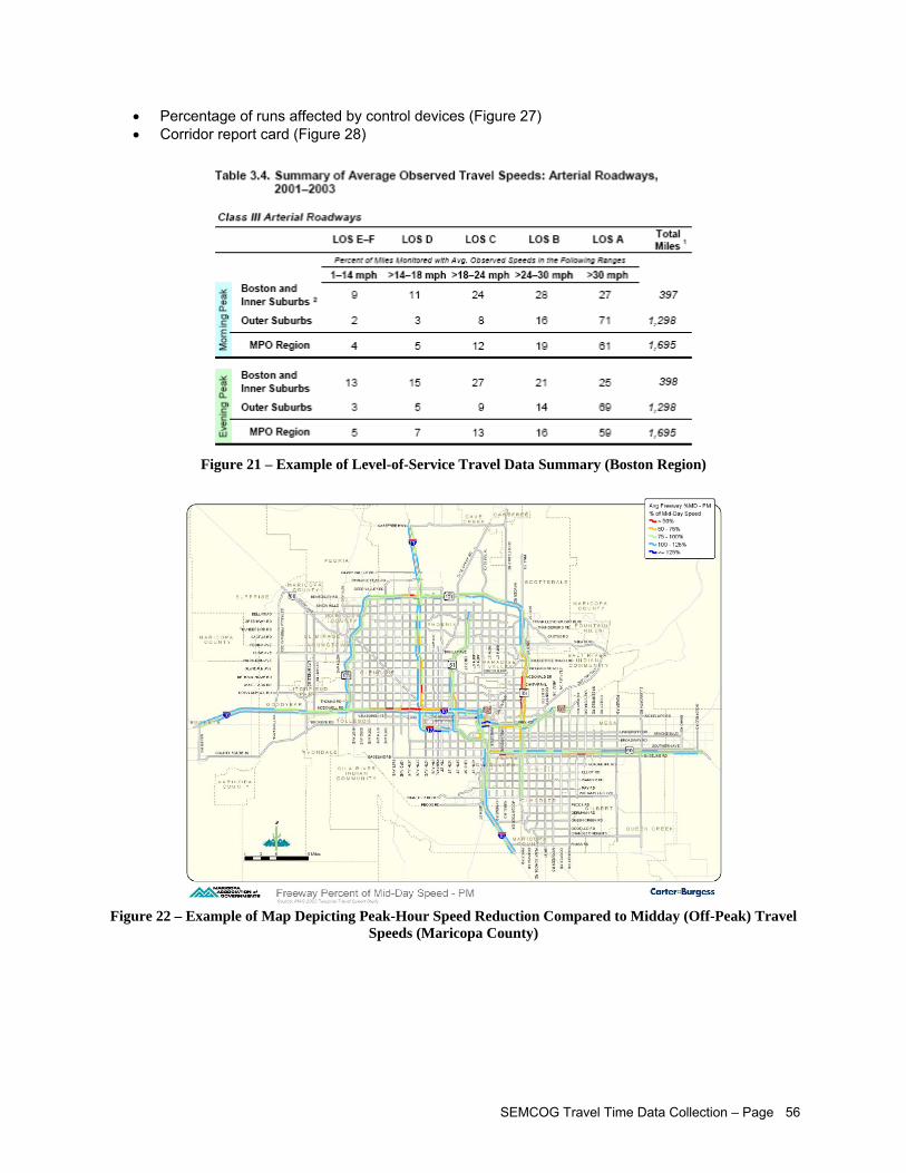
SEMCOG Travel Time Data Collection – Page 56
• Percentage of runs affected by control devices (Figure 27) • Corridor report card (Figure 28)
Figure 21 – Example of Level-of-Service Travel Data Summary (Boston Region)
Figure 22 – Example of Map Depicting Peak-Hour Speed Reduction Compared to Midday (Off-Peak) Travel
Speeds (Maricopa County)
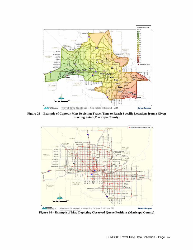
SEMCOG Travel Time Data Collection – Page 57
Figure 23 – Example of Contour Map Depicting Travel Time to Reach Specific Locations from a Given
Starting Point (Maricopa County)
Figure 24 – Example of Map Depicting Observed Queue Positions (Maricopa County)
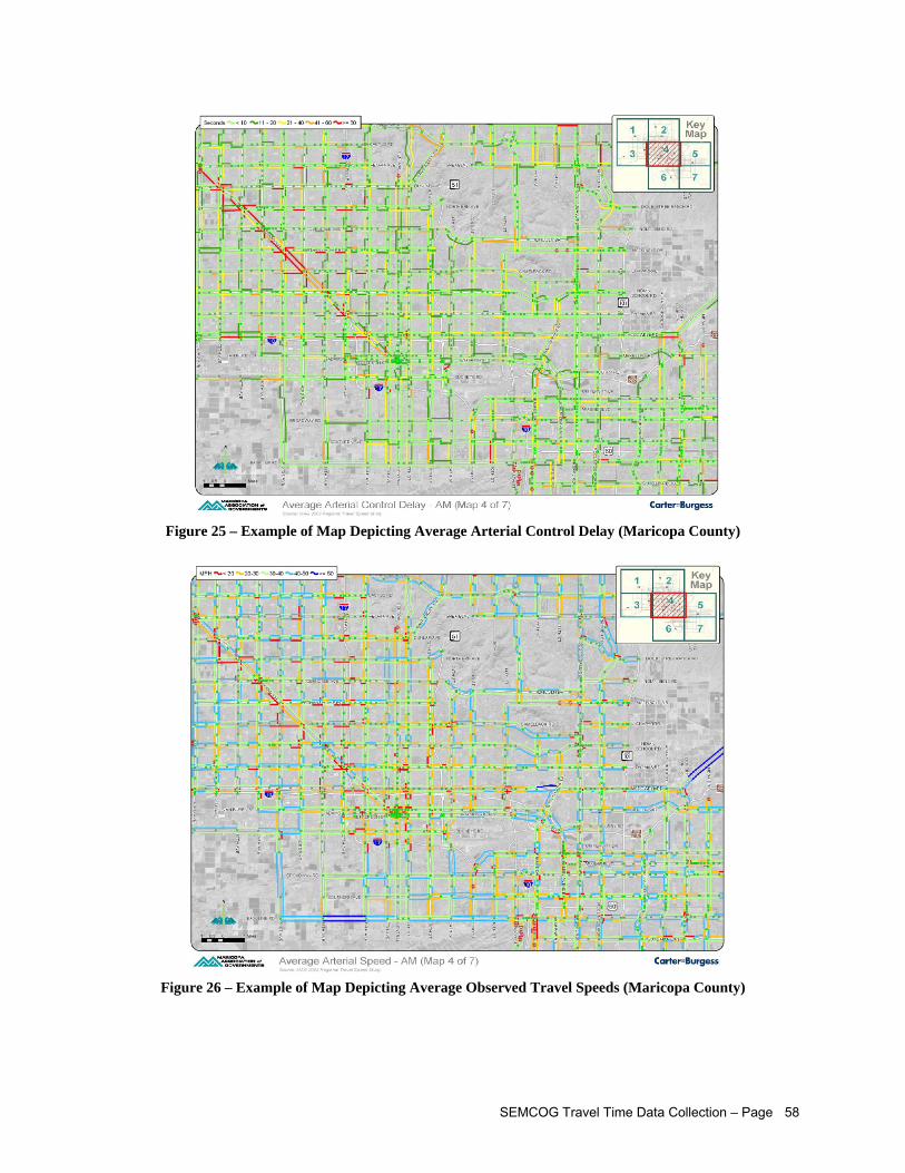
SEMCOG Travel Time Data Collection – Page 58
Figure 25 – Example of Map Depicting Average Arterial Control Delay (Maricopa County)
Figure 26 – Example of Map Depicting Average Observed Travel Speeds (Maricopa County)
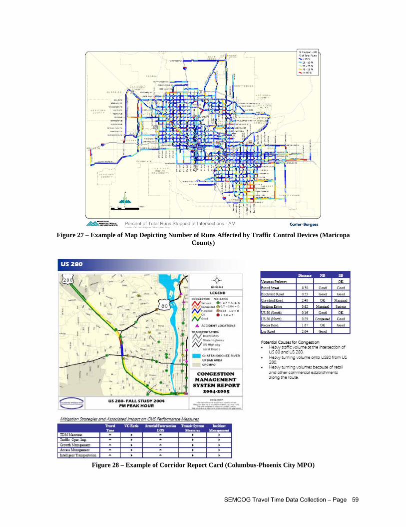
SEMCOG Travel Time Data Collection – Page 59
Figure 27 – Example of Map Depicting Number of Runs Affected by Traffic Control Devices (Maricopa
County)
Figure 28 – Example of Corridor Report Card (Columbus-Phoenix City MPO)
SEMCOG Travel Time Data Collection – Page 60
10.3 Recommended Data Reporting
Based on current reporting practice, it is recommended that at a minimum the following information be compiled and reported:
• Table providing average observed travel time, travel time variability, average delay and average number of stops for all major travel corridors
• Network graph illustrating average observed travel speeds on a segment-by-segment basis • Network graph illustrating average observed segment delays on a segment-by-segment basis • Network graph illustrating assessed levels of service on a segment-by-segment basis
SEMCOG Travel Time Data Collection – Page 61
11 Estimation of Travel Time Parameters This section provides methods for estimating travel parameters from second-by-second speed and acceleration data typically obtained from travel time runs. Parameter estimation techniques covered in this section include:
• Cumulative Traveled distance • Vehicle acceleration rates • Free-flow speed • Average speed • Running speed • Number of stops • Segment delay • Stopped delay • Control delay • Approach delay
While many of the explanations are provided with respect to segment delimited by signalized intersections, as such delimitations are the most common, the same definitions can be applied to segments delimited by arbitrary reference points.
11.1 Cumulative Traveled Distance
GPS equipment typically provides speed and position measurements in an X-Y grid. To be of greatest use, the position measurement must be converted into linear travel distance measurements.
In some cases, such measurements can be directly obtained from a DMI installed on the test vehicle. If the GPS and DMI time clocks are coordinated, it is then relatively easy to link the DMI recordings to the GPS measurements and obtained the desired information.
If direct distance measurements are not available, traveled distances must be extracted from the position measurements. If a vehicle’s position is measured using the Universal Transverse Mercator (UTM) coordinate system, the X and Y coordinates then represent the location of a vehicle on a flat grid with perpendicular axes with respect to a fixed reference point. Since GPS coordinate measurements are in meters, the linear distance traveled by a vehicle between two measurements could be assessed using Equation 32:
( ) ( )212
128084.3 −− −+−=∆ iiiii yyxxL [32]
Where: ∆Li = Linear distance traveled between data points i-1 and i (feet) xi = Recorded x coordinate at data point i yi = Recorded y coordinate at data point i
If measurements are made using another reference grid, an appropriate conversion formula must then be used to extract distances traveled from the measured x and y coordinates.
Equation 32 measures straight distances between two coordinates. Discrepancies may thus exist between actual traveled distances and calculated distances when a vehicle is not traveling in a straight line, such as along a curve. However, use of Equation 26 should provide reasonably accurate distance measurements when applied to the processing of second-by-second data given the relatively small traveled distances that then normally exist between each position measurement.
Using Equation 32, the location of a vehicle along a roadway segment at any given moment can be determined using Equation 33 as a simple summation of assessed traveled distances between each pair of successive data points.
SEMCOG Travel Time Data Collection – Page 62
∑=
∆=i
mmi LL
2
[33]
Where: Li = Linear location of vehicle at data point i (feet) ∆Lm = Linear distance traveled between data points m-1 and m (feet)
11.2 Vehicle Acceleration Rates
In the simplest case, observed vehicle acceleration/deceleration rates can be calculated using a backward difference approach as per Equation 34. This approach estimates a vehicle’s acceleration at a given time using current speed and immediately preceding recorded data.
1
1 −
−
−−
=ii
iii tt
ssa [34]
Where: ai = Acceleration at data point i si = Speed of vehicle at data point i ti = Time associated with data point i
However, a generally preferred approach is to calculate accelerations using a central difference approach. In this simplest form, this means calculating accelerations using data points i-1 and i+1, as per Equation 35. This approach is generally preferred as application of central difference scheme has generally been shown to produce estimated values that are one order of magnitude more accurate than values estimated using either backward or forward difference schemes.
11
11 −+
−+
−−
=ii
iii tt
ssa [35]
Where: ai = Acceleration at data point i si = Speed of vehicle at data point i ti = Time associated with data point i
11.3 Free Flow Speed
Free-flow speed occurs when volumes are low and drivers are not influenced by the presence of other vehicles or traffic control devices. This speed theoretically represents the maximum average speed at which traffic will typically travel on a roadway segment in the absence of any impeding factors other than roadway geometry.
A common approach to measure free-flow speed is to measure travel times during periods of light traffic. One recommendation suggested by Hoeschen et al. (2005) is to collect data when traffic volumes are less than 200 vehicles per hour per lane. Depending on the segment considered this may correspond to a mid-morning, mid-afternoon, evening or weekend period.
One potential problem in obtaining free-flow travel information through direct field measurement is that this approach may yield speeds above posted speed limits. In such a situation, the assessment of free-flow speed and free-flow travel time are often capped to values that would be obtained if traffic were actually following speed limits. The rationale for capping calculations is that congestion should only be measured with respect to the legal speed limit on each segment since these limits define the minimum travel time for which each segment is intended to operate in the absence of congestion.
11.4 Average Speed
The average speed is simply the ratio of the total distance traveled over the total time taken to travel the distance. It is a measure of how fast a vehicle is progressing along a segment when factoring all the delays imposed by other vehicles and traffic control devices. In the illustrated space-time trajectory of
SEMCOG Travel Time Data Collection – Page 63
Figure 29, the average speed would be estimated using Equation 36, arbitrarily assuming that the center points of intersections A and B mark the start and end of the segment under consideration.
05
05
ttLLsavg −
−= [36]
Where: savg = Average speed L0 = Center of upstream intersection L5 = Center of downstream intersection t0 = Time when vehicle is at center of upstream intersection t5 = Time when vehicle is at center of downstream intersection
When processing second-by-second data, Equation 36 converts to Equation 37:
⎟⎟⎟⎟⎟⎟
⎠
⎞
⎜⎜⎜⎜⎜⎜
⎝
⎛
−
−
=
⎟⎟⎟⎟⎟⎟
⎠
⎞
⎜⎜⎜⎜⎜⎜
⎝
⎛
−
∆
=
⎟⎟⎠
⎞⎜⎜⎝
⎛
−
−=
∑
∑
∑
=−
=−
=
k
k
k
k
k
k
n
iii
n
iii
n
n
ii
n
nkavg
tt
LL
tt
L
ttLL
s
21
21
1
2
1
1
46667.11
46667.11
46667.11
[37]
Where: savg k = Average speed over segment k (mph) nk = Number of data points associated with segment k ∆Li = Linear distance traveled between data points i-1 and i (feet) Li = Linear location of vehicle at data point i (feet) ti = Time associated with data point i (seconds)
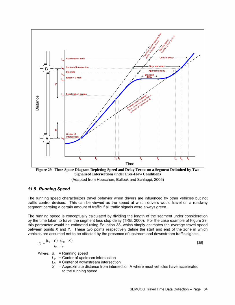
SEMCOG Travel Time Data Collection – Page 64
Figure 29 –Time-Space Diagram Depicting Speed and Delay Terms on a Segment Delimited by Two Signalized Intersections under Free-Flow Conditions
(Adapted from Hoeschen, Bullock and Schlappi, 2005)
11.5 Running Speed
The running speed characterizes travel behavior when drivers are influenced by other vehicles but not traffic control devices. This can be viewed as the speed at which drivers would travel on a roadway segment carrying a certain amount of traffic if all traffic signals were always green.
The running speed is conceptually calculated by dividing the length of the segment under consideration by the time taken to travel the segment less stop delay (TRB, 2000). For the case example of Figure 29, this parameter would be estimated using Equation 38, which simply estimates the average travel speed between points X and Y. These two points respectively define the start and end of the zone in which vehicles are assumed not to be affected by the presence of upstream and downstream traffic signals.
( ) ( )XY
r ttXLYLs
−−−−
= 05 [38]
Where: sr = Running speed L0 = Center of upstream intersection L5 = Center of downstream intersection X = Approximate distance from intersection A where most vehicles have accelerated
to the running speed
B
A
B
A L0
L1
L2
L4
L5
L6
X
Y
t0 tX t1tY t2 t3 t4 t5 t6
Acceleration ends
Center of intersection
Stop line
Speed = 0 mph
Deceleration begins
Center of intersection
Stoppeddelay
Approach delay
Segment delay
Control delayFree
-flow
spee
d tra
jecto
ryfro
m
cent
er o
f inte
rsec
tion
ARun
ning s
peed
trajec
tory
from
point
X
Average speed trajectory
from center of interse
ction A
to center of intersection B
Time
Dis
tanc
e
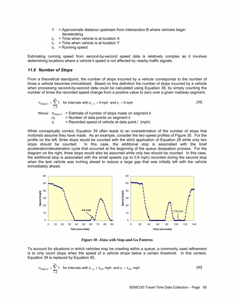
SEMCOG Travel Time Data Collection – Page 65
Y = Approximate distance upstream from intersection B where vehicles begin decelerating
tX = Time when vehicle is at location X tY = Time when vehicle is at location Y sr = Running speed
Estimating running speed from second-by-second speed data is relatively complex as it involves determining locations where a vehicle’s speed is not affected by nearby traffic signals.
11.6 Number of Stops
From a theoretical standpoint, the number of stops incurred by a vehicle corresponds to the number of times a vehicle becomes immobilized. Based on this definition the number of stops incurred by a vehicle when processing second-by-second data could be calculated using Equation 39, by simply counting the number of times the recorded speed change from a positive value to zero over a given roadway segment.
mph 0 and mph 0 withintervals for 12
=>= −=∑ i1i
n
ikstops ssn
k
[39]
Where: nstops k = Estimate of number of stops made on segment k nk = Number of data points on segment k si = Recorded speed of vehicle at data point i (mph)
While conceptually correct, Equation 39 often leads to an overestimation of the number of stops that motorists assume they have made. As an example, consider the two speed profiles of Figure 30. For the profile on the left, three stops would be counted with the strict application of Equation 28 while only two stops should be counted. In this case, the additional stop is associated with the brief acceleration/deceleration cycle that occurred at the beginning of the queue dissipation process. For the diagram on the right, three stops would also be assumed while only two should be counted. In this case, the additional stop is associated with the small speeds (up to 0.8 mph) recorded during the second stop when the test vehicle was inching ahead to reduce a large gap that was initially left with the vehicle immediately ahead.
0
10
20
30
40
50
60
0 10 20 30 40 50 60 70 80 90
Time (seconds)
Spee
d (m
ph)
4.9 mph
0
10
20
30
40
50
60
0 20 40 60 80 100 120 140
Time (seconds)
Spee
d (m
ph)
0.8 mph
Figure 30 –Data with Stop-and-Go Patterns
To account for situations in which vehicles may be crawling within a queue, a commonly used refinement is to only count stops when the speed of a vehicle drops below a certain threshold. In this context, Equation 39 is replaced by Equation 40.
mph and mph withintervals for 12
refiref1i
n
ikstops ssssn
k
<≥= −=∑ [40]
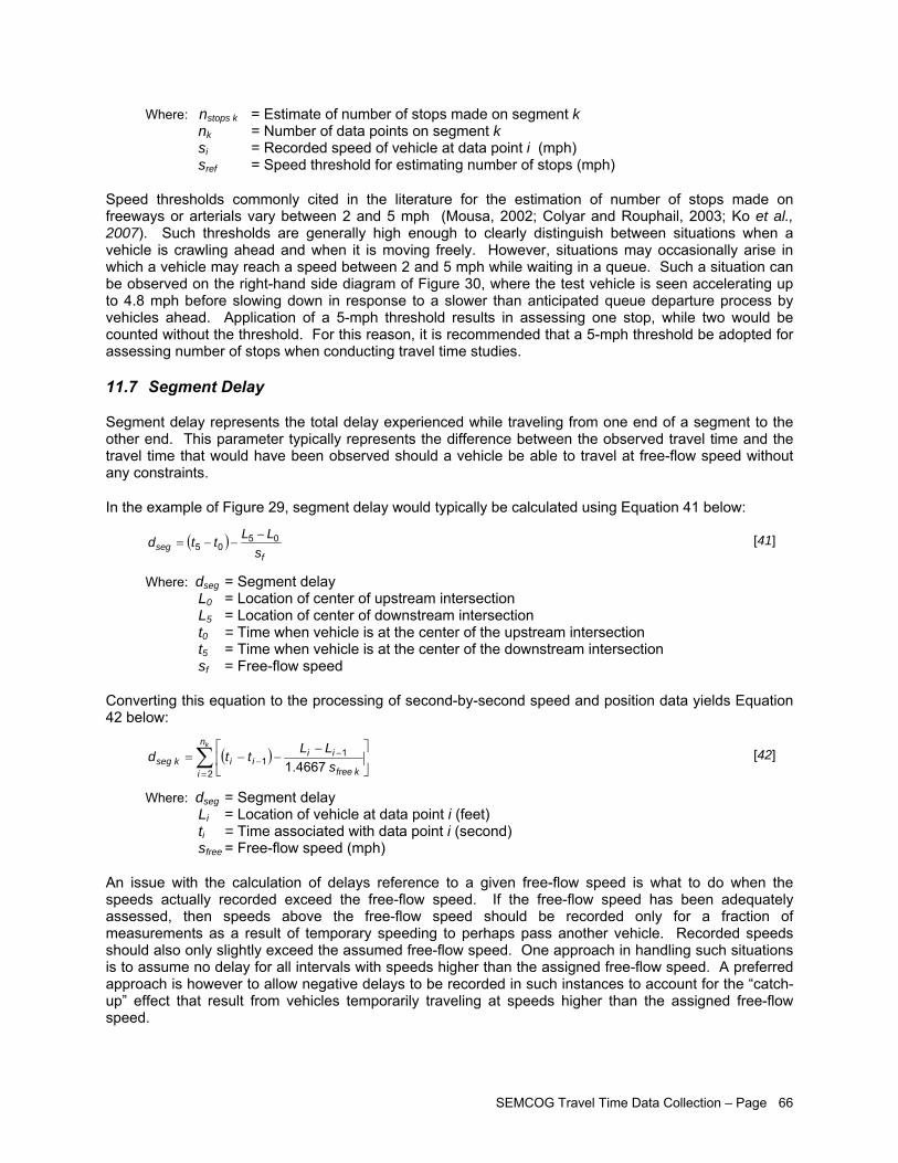
SEMCOG Travel Time Data Collection – Page 66
Where: nstops k = Estimate of number of stops made on segment k nk = Number of data points on segment k si = Recorded speed of vehicle at data point i (mph) sref = Speed threshold for estimating number of stops (mph)
Speed thresholds commonly cited in the literature for the estimation of number of stops made on freeways or arterials vary between 2 and 5 mph (Mousa, 2002; Colyar and Rouphail, 2003; Ko et al., 2007). Such thresholds are generally high enough to clearly distinguish between situations when a vehicle is crawling ahead and when it is moving freely. However, situations may occasionally arise in which a vehicle may reach a speed between 2 and 5 mph while waiting in a queue. Such a situation can be observed on the right-hand side diagram of Figure 30, where the test vehicle is seen accelerating up to 4.8 mph before slowing down in response to a slower than anticipated queue departure process by vehicles ahead. Application of a 5-mph threshold results in assessing one stop, while two would be counted without the threshold. For this reason, it is recommended that a 5-mph threshold be adopted for assessing number of stops when conducting travel time studies.
11.7 Segment Delay
Segment delay represents the total delay experienced while traveling from one end of a segment to the other end. This parameter typically represents the difference between the observed travel time and the travel time that would have been observed should a vehicle be able to travel at free-flow speed without any constraints.
In the example of Figure 29, segment delay would typically be calculated using Equation 41 below:
( )f
seg sLLttd 05
05−
−−= [41]
Where: dseg = Segment delay L0 = Location of center of upstream intersection L5 = Location of center of downstream intersection t0 = Time when vehicle is at the center of the upstream intersection t5 = Time when vehicle is at the center of the downstream intersection sf = Free-flow speed
Converting this equation to the processing of second-by-second speed and position data yields Equation 42 below:
( )∑=
−− ⎥
⎦
⎤⎢⎣
⎡ −−−=
kn
i kfree
iiiikseg s
LLttd2
11 4667.1
[42]
Where: dseg = Segment delay Li = Location of vehicle at data point i (feet) ti = Time associated with data point i (second) sfree = Free-flow speed (mph)
An issue with the calculation of delays reference to a given free-flow speed is what to do when the speeds actually recorded exceed the free-flow speed. If the free-flow speed has been adequately assessed, then speeds above the free-flow speed should be recorded only for a fraction of measurements as a result of temporary speeding to perhaps pass another vehicle. Recorded speeds should also only slightly exceed the assumed free-flow speed. One approach in handling such situations is to assume no delay for all intervals with speeds higher than the assigned free-flow speed. A preferred approach is however to allow negative delays to be recorded in such instances to account for the “catch-up” effect that result from vehicles temporarily traveling at speeds higher than the assigned free-flow speed.
SEMCOG Travel Time Data Collection – Page 67
11.8 Stopped Delay
Stopped delay measures the amount of time a vehicle is physically stopped. In most cases, this will correspond to time spent waiting in a queue at an intersection. Since stopped delay can easily be measured with the use of a simple stopwatch, this parameter was the primary measure used to characterize traffic control operations up until the late 1980s. Since then, this parameter has been replaced by the control delay.
For the case example of Figure 29, stopped delay is graphically represented by the flat portion between points 2 and 3 on the illustrated vehicle trajectory. This can be expressed mathematically by:
23 ttds −= [43]
Where: ds = Stopped delay t2 = Time when speed decreases below selected threshold t3 = Time when speed increases above selected threshold
While the concept of stopped delay is easily defined, estimating this parameter from second-by-second travel data is subject to some interpretation. From a strict standpoint, stopped delay can be estimated from such data by simply summing the time intervals during which a vehicle is has a speed of 0 mph, as per Equation 44.
( ) mph 0 withintervals all for 2
1 =−= ∑=
− i
n
iiikstop sttd
k
[44]
Where: dstop k = Stopped delay (seconds) ti = Time associated with data point i (seconds) si = Speed recorded at data point i (mph) nk = Number of data points on roadway segment k
However, a problem with the simple summation of intervals with speed of 0 mph exists when vehicles do not remain fully immobilized while waiting in a queue. Vehicles are often observed to gradually close the gap between the vehicles immediately ahead by inching forward after an initial stop. Often, this movement will be sufficient to cause a small speed to be recorded for some intervals, thus resulting in these intervals not being counted for stopped delay as they should.
To remove the above problem, a commonly used approach is to consider that a vehicle is stopped if its speed is below some predefined threshold, as shown in Equation 45. Thresholds commonly reported in the literature vary between 2 and 5 mph. For instance, the Maricopa County Association of Governments in Arizona recently requested in a request for proposals that stopped delay must be calculated by considering intervals with speeds of less than 3 mph.
( ) refi
n
i kfree
iiiikstop ss
sLLttd
k
<⎥⎦
⎤⎢⎣
⎡ −−−= ∑
=
−− withintervals all for
4667.12
11 [45]
Where: dstop k = Stopped delay (seconds) si = Recorded speed of vehicle at data point i (mph) sref = Threshold speed for calculation of stopped delay (mph) sfree k = Free-flow speed on segment k (mph) Li = Location of vehicle at data point i (feet) ti = Time associated with data point i (seconds) nk = Number of data points on roadway segment
Speeds between 2 and 5 mph are generally low enough to provide a clear distinction between a vehicle waiting in a queue, and a vehicle progressing along a roadway segment. Vehicles would not normally travel at such low speeds when not constrained by queued vehicles. However, it is possible that, on occasion, speeds between 2 and 5 mph are recorded while vehicles are still technically waiting in a queue. Consider for instance the profile illustrated on left side of Figure 30, where a vehicle is seen accelerating
SEMCOG Travel Time Data Collection – Page 68
to 4.8 mph while anticipating the start of the upcoming green. To account for such situations, it is highly recommended to use a 5 mph threshold for assessing stopped delay.
11.9 Control Delay
Control delay is the delay experienced by a vehicle when progressing through a section of road influenced by a traffic signal. It is more inclusive than stopped delay as it includes delays experienced while decelerating, being stopped at the intersection, and accelerating back to a given running speed downstream of the intersection. In the diagram of Figure 29, control delay would be conceptually estimated using Equation 46:
( )r
c sLLttd 16
16−
−−= [46]
Where: dc = Control delay t1 = Time when deceleration begins t6 = Time when acceleration ends L1 = Location where deceleration begins L6 = Location where acceleration ends sr = Running speed
Control delay is generally thought to be a better indicator of the of the impact of traffic control devices on traffic since it reflects the entire delay imposed on motorists by a control device and not just the duration during which a vehicle is stopped. This accounts for situations in which a vehicle may slow down but not reach a full stop. For this reason, control delay has now generally replaced stopped delay as the primary measure to assess delays at intersections (TRB, 2000).
A common assumption when comparing stopped and control delays is that control delay is approximately 30% greater than stopped delay. While this approximation was confirmed to be generally valid by a study conducted at Louisiana State University (Quiroga and Bullock, 1998b, 1999), the study also demonstrated that secondary effects due to signal cycle and offset make the relation between stopped and control delays more complicated than a simple linear multiplier, thus throwing caution in using the 30% conversion factor mentioned in the literature.
The difficulty in estimating control delay using second-by-second data, is identifying when a vehicle starts decelerating in response to an approaching control device (moment t1 in Figure 29) and when it stops accelerating on the other side of the device after it has reached its desired speed (moment t6 in Figure 29). Because of the potential variations in driver behavior, complex algorithms are required to analyze recorded speed profiles. This is a topic that is still subject to research (see for instance work by Quiroga and Bullock (1999), Colyar and Rouphail (2003), and Ko et al. (2007).
The following describes a simple procedure that can be used to assess control delay on roadway segments with relatively simple speed profiles. More complex algorithms may be needed to correctly handle profiles without clear boundaries between deceleration/acceleration cycles due to interactions with a traffic control device and random deceleration/acceleration events attributed to driver behavior and other traffic effects. Similar to many proposed methodologies, the procedure requires several input elements:
• Desired or free-flow travel speed (sfree) on segments upstream and downstream of intersection • Smoothed second-by-second speed profile • Second-by-second acceleration profile • Location of intersection’s stop line • Location of test vehicle associated with each data point in speed profile
Using Figure 31 as reference, control delay can be estimated by applying the following steps:
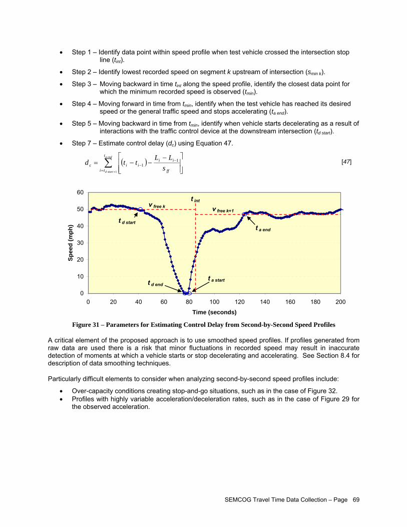
SEMCOG Travel Time Data Collection – Page 69
• Step 1 – Identify data point within speed profile when test vehicle crossed the intersection stop line (tint).
• Step 2 – Identify lowest recorded speed on segment k upstream of intersection (smin k).
• Step 3 – Moving backward in time tint along the speed profile, identify the closest data point for which the minimum recorded speed is observed (tmin).
• Step 4 – Moving forward in time from tmin, identify when the test vehicle has reached its desired speed or the general traffic speed and stops accelerating (ta end).
• Step 5 – Moving backward in time from tmin, identify when vehicle starts decelerating as a result of interactions with the traffic control device at the downstream intersection (td start).
• Step 7 – Estimate control delay (dc) using Equation 47.
( )∑+=
−−
⎥⎥⎦
⎤
⎢⎢⎣
⎡ −−−=
a end
startd
t
ti ff
iiiic s
LLttd
1
11
[47]
0
10
20
30
40
50
60
0 20 40 60 80 100 120 140 160 180 200
Time (seconds)
Spee
d (m
ph)
v free k v free k+1
t d start
t d endt a start
t a end
t int
Figure 31 – Parameters for Estimating Control Delay from Second-by-Second Speed Profiles
A critical element of the proposed approach is to use smoothed speed profiles. If profiles generated from raw data are used there is a risk that minor fluctuations in recorded speed may result in inaccurate detection of moments at which a vehicle starts or stop decelerating and accelerating. See Section 8.4 for description of data smoothing techniques.
Particularly difficult elements to consider when analyzing second-by-second speed profiles include:
• Over-capacity conditions creating stop-and-go situations, such as in the case of Figure 32. • Profiles with highly variable acceleration/deceleration rates, such as in the case of Figure 29 for
the observed acceleration.
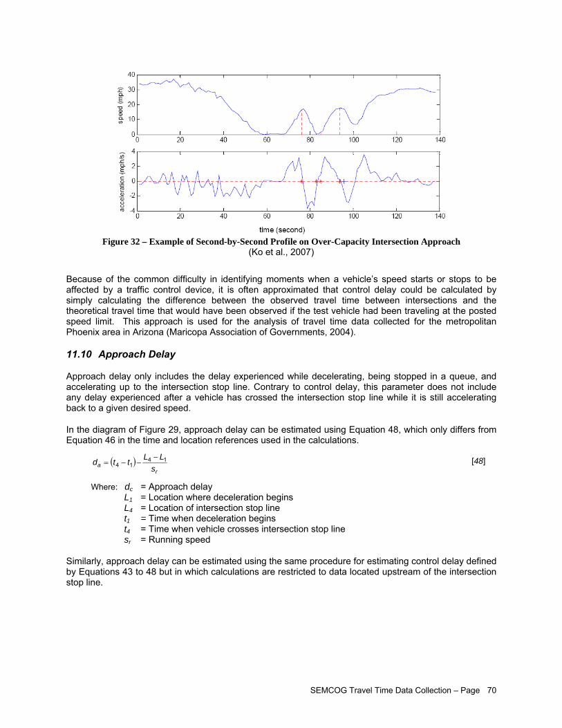
SEMCOG Travel Time Data Collection – Page 70
Figure 32 – Example of Second-by-Second Profile on Over-Capacity Intersection Approach
(Ko et al., 2007)
Because of the common difficulty in identifying moments when a vehicle’s speed starts or stops to be affected by a traffic control device, it is often approximated that control delay could be calculated by simply calculating the difference between the observed travel time between intersections and the theoretical travel time that would have been observed if the test vehicle had been traveling at the posted speed limit. This approach is used for the analysis of travel time data collected for the metropolitan Phoenix area in Arizona (Maricopa Association of Governments, 2004).
11.10 Approach Delay
Approach delay only includes the delay experienced while decelerating, being stopped in a queue, and accelerating up to the intersection stop line. Contrary to control delay, this parameter does not include any delay experienced after a vehicle has crossed the intersection stop line while it is still accelerating back to a given desired speed.
In the diagram of Figure 29, approach delay can be estimated using Equation 48, which only differs from Equation 46 in the time and location references used in the calculations.
( )r
a sLLttd 14
14−
−−= [48]
Where: dc = Approach delay L1 = Location where deceleration begins L4 = Location of intersection stop line t1 = Time when deceleration begins t4 = Time when vehicle crosses intersection stop line sr = Running speed
Similarly, approach delay can be estimated using the same procedure for estimating control delay defined by Equations 43 to 48 but in which calculations are restricted to data located upstream of the intersection stop line.
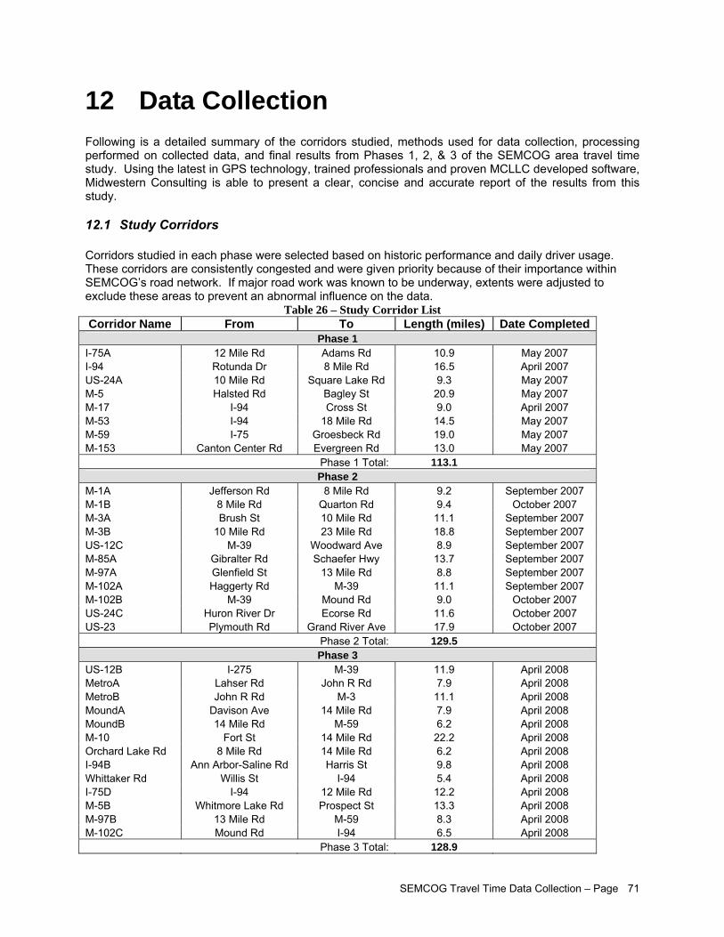
SEMCOG Travel Time Data Collection – Page 71
12 Data Collection Following is a detailed summary of the corridors studied, methods used for data collection, processing performed on collected data, and final results from Phases 1, 2, & 3 of the SEMCOG area travel time study. Using the latest in GPS technology, trained professionals and proven MCLLC developed software, Midwestern Consulting is able to present a clear, concise and accurate report of the results from this study.
12.1 Study Corridors Corridors studied in each phase were selected based on historic performance and daily driver usage. These corridors are consistently congested and were given priority because of their importance within SEMCOG’s road network. If major road work was known to be underway, extents were adjusted to exclude these areas to prevent an abnormal influence on the data.
Table 26 – Study Corridor List Corridor Name From To Length (miles) Date Completed
Phase 1 I-75A 12 Mile Rd Adams Rd 10.9 May 2007 I-94 Rotunda Dr 8 Mile Rd 16.5 April 2007 US-24A 10 Mile Rd Square Lake Rd 9.3 May 2007 M-5 Halsted Rd Bagley St 20.9 May 2007 M-17 I-94 Cross St 9.0 April 2007 M-53 I-94 18 Mile Rd 14.5 May 2007 M-59 I-75 Groesbeck Rd 19.0 May 2007 M-153 Canton Center Rd Evergreen Rd 13.0 May 2007 Phase 1 Total: 113.1
Phase 2 M-1A Jefferson Rd 8 Mile Rd 9.2 September 2007 M-1B 8 Mile Rd Quarton Rd 9.4 October 2007 M-3A Brush St 10 Mile Rd 11.1 September 2007 M-3B 10 Mile Rd 23 Mile Rd 18.8 September 2007 US-12C M-39 Woodward Ave 8.9 September 2007 M-85A Gibralter Rd Schaefer Hwy 13.7 September 2007 M-97A Glenfield St 13 Mile Rd 8.8 September 2007 M-102A Haggerty Rd M-39 11.1 September 2007 M-102B M-39 Mound Rd 9.0 October 2007 US-24C Huron River Dr Ecorse Rd 11.6 October 2007 US-23 Plymouth Rd Grand River Ave 17.9 October 2007 Phase 2 Total: 129.5
Phase 3 US-12B I-275 M-39 11.9 April 2008 MetroA Lahser Rd John R Rd 7.9 April 2008 MetroB John R Rd M-3 11.1 April 2008 MoundA Davison Ave 14 Mile Rd 7.9 April 2008 MoundB 14 Mile Rd M-59 6.2 April 2008 M-10 Fort St 14 Mile Rd 22.2 April 2008 Orchard Lake Rd 8 Mile Rd 14 Mile Rd 6.2 April 2008 I-94B Ann Arbor-Saline Rd Harris St 9.8 April 2008 Whittaker Rd Willis St I-94 5.4 April 2008 I-75D I-94 12 Mile Rd 12.2 April 2008 M-5B Whitmore Lake Rd Prospect St 13.3 April 2008 M-97B 13 Mile Rd M-59 8.3 April 2008 M-102C Mound Rd I-94 6.5 April 2008 Phase 3 Total: 128.9
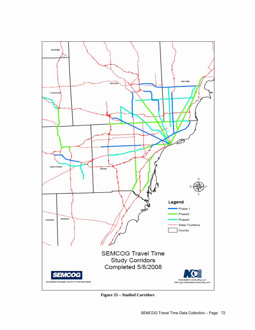
SEMCOG Travel Time Data Collection – Page 72
Figure 33 – Studied Corridors
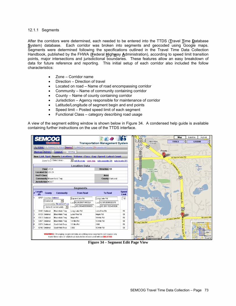
SEMCOG Travel Time Data Collection – Page 73
12.1.1 Segments After the corridors were determined, each needed to be entered into the TTDS (Travel Time Database System) database. Each corridor was broken into segments and geocoded using Google maps. Segments were determined following the specifications outlined in the Travel Time Data Collection Handbook, published by the FHWA (Federal Highway Administration), according to speed limit transition points, major intersections and jurisdictional boundaries. These features allow an easy breakdown of data for future reference and reporting. This initial setup of each corridor also included the follow characteristics:
• Zone – Corridor name • Direction – Direction of travel • Located on road – Name of road encompassing corridor • Community – Name of community containing corridor • County – Name of county containing corridor • Jurisdiction – Agency responsible for maintenance of corridor • Latitude/Longitude of segment begin and end points • Speed limit – Posted speed limit of each segment • Functional Class – category describing road usage
A view of the segment editing window is shown below in Figure 34. A condensed help guide is available containing further instructions on the use of the TTDS interface.
Figure 34 – Segment Edit Page View
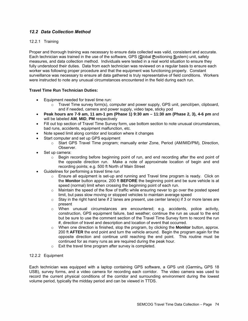
SEMCOG Travel Time Data Collection – Page 74
12.2 Data Collection Method
12.2.1 Training Proper and thorough training was necessary to ensure data collected was valid, consistent and accurate. Each technician was trained in the use of the software, GPS (Global Positioning System) unit, safety measures, and data collection method. Individuals were tested in a real world situation to ensure they fully understood their duties. Data from each technician was reviewed on a regular basis to ensure each worker was following proper procedure and that the equipment was functioning properly. Constant surveillance was necessary to ensure all data gathered is truly representative of field conditions. Workers were instructed to note any unusual circumstances encountered in the field during each run. Travel Time Run Technician Duties:
• Equipment needed for travel time run: o Travel Time survey form(s), computer and power supply, GPS unit, pencil/pen, clipboard,
and if needed, camera and power supply, video tape, sticky pod • Peak hours are 7-9 am, 11 am-1 pm (Phase 1) 9:30 am – 11:30 am (Phase 2, 3), 4-6 pm and
will be labeled AM, MID, PM respectively • Fill out top section of Travel Time Survey form, use bottom section to note unusual circumstances,
bad runs, accidents, equipment malfunction, etc. • Note speed limit along corridor and location where it changes • Start computer and set up GPS equipment
o Start GPS Travel Time program; manually enter Zone, Period (AM/MID/PM), Direction, Observer.
• Set up camera: o Begin recording before beginning point of run, and end recording after the end point of
the opposite direction run. Make a note of approximate location of begin and end recording points; e.g. 500 ft North of Main Street
• Guidelines for performing a travel time run o Ensure all equipment is set-up and running and Travel time program is ready. Click on
the Monitor button approx. 200 ft BEFORE the beginning point and be sure vehicle is at speed (normal) limit when crossing the beginning point of each run.
o Maintain the speed of the flow of traffic while ensuring never to go over the posted speed limit, but pass slow moving or stopped vehicles to maintain average speed
o Stay in the right hand lane if 2 lanes are present, use center lane(s) if 3 or more lanes are present
o When unusual circumstances are encountered; e.g. accidents, police activity, construction, GPS equipment failure, bad weather; continue the run as usual to the end but be sure to use the comment section of the Travel Time Survey form to record the run #, direction of travel and description and location of event that occurred.
o When one direction is finished, stop the program, by clicking the Monitor button, approx. 200 ft AFTER the end point and turn the vehicle around. Begin the program again for the opposite direction and continue until reaching the end point. This routine must be continued for as many runs as are required during the peak hour.
o Exit the travel time program after survey is completed.
12.2.2 Equipment Each technician was equipped with a laptop containing GPS software, a GPS unit (Garmin® GPS 18 USB), survey forms, and a video camera for recording each corridor. The video camera was used to record the current physical conditions of the corridor and surrounding environment during the lowest volume period, typically the midday period and can be viewed in TTDS.
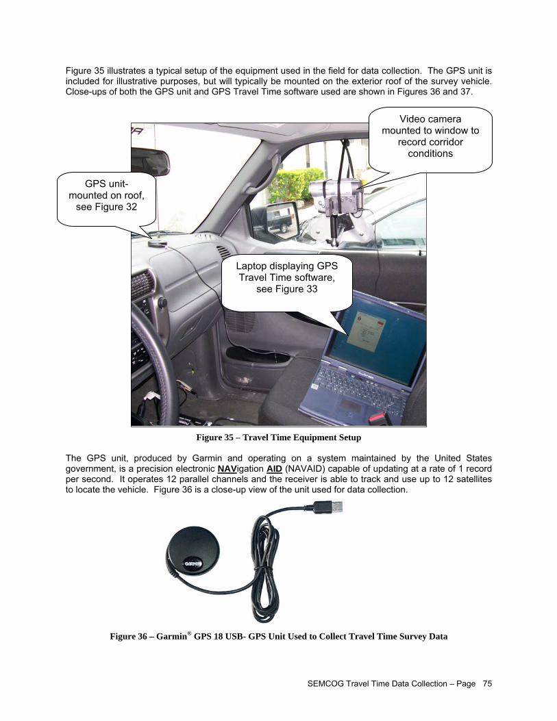
SEMCOG Travel Time Data Collection – Page 75
Figure 35 illustrates a typical setup of the equipment used in the field for data collection. The GPS unit is included for illustrative purposes, but will typically be mounted on the exterior roof of the survey vehicle. Close-ups of both the GPS unit and GPS Travel Time software used are shown in Figures 36 and 37.
Figure 35 – Travel Time Equipment Setup The GPS unit, produced by Garmin and operating on a system maintained by the United States government, is a precision electronic NAVigation AID (NAVAID) capable of updating at a rate of 1 record per second. It operates 12 parallel channels and the receiver is able to track and use up to 12 satellites to locate the vehicle. Figure 36 is a close-up view of the unit used for data collection.
Figure 36 – Garmin® GPS 18 USB- GPS Unit Used to Collect Travel Time Survey Data
GPS unit- mounted on roof,
see Figure 32
Video camera mounted to window to
record corridor conditions
Laptop displaying GPS Travel Time software,
see Figure 33
SEMCOG Travel Time Data Collection – Page 76
The GPS Travel Time program grabs data from the GPS unit every second. The data is then parsed out to a NMEA (National Marine Electronics Association) 0183 standard text file created for every run.
12.2.3 Method State of the practice research covered in detail in previous sections of this report determined that the floating car method, average car method or a hybrid of these two methods is the most widely used and statistically reasonable test vehicle method during a travel time data collection project. These two methods require the technician to pass vehicles regardless of the speed limit on each segment of roadway. During the data processing, it is necessary to remove all data points that show the vehicle going over the speed limit. Because of this, all field workers were instructed to maintain the posted speed limit whenever possible, and pass slow or blocking vehicles in order to maintain the speed limit. For safety reasons, drivers were instructed to stay in the right or center lane when possible to avoid creating a driving hazard. The GPS unit was positioned on the roof of the car and attached via USB port to the laptop inside the vehicle. The GPS Travel Time program is used to create a filename of each run and parse available data to obtain specific required data. NMEA standard data is recorded from the data stream obtained through the GPS unit. This data is recorded every second and parsed out to the text files created for every run. The following list details the data recorded every second:
• X Value – Longitude (WGS 84 Coordinate System) • Y Value – Latitude (WGS 84 Coordinate System) • Number of Satellites – Number of satellites detected by the GPS unit, up to 12 • HDOP (Horizontal Dilution of Precision) - Horizontal accuracy of 2-D coordinates,
indicator of quality of geometry of satellite. A greater angle between satellites provides a better measurement. A value less than 4 is good or larger than 8 is bad.
• Speed – Traveling speed of vehicle, mph • Timestamp - System time of each recorded second of data
Figure 37 is a view of the GPS Travel Time program used in conjunction with the GPS unit to capture second-by-second data for each corridor.
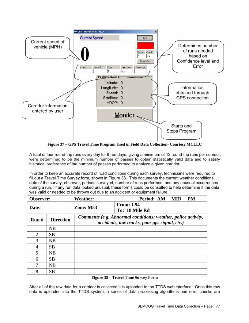
SEMCOG Travel Time Data Collection – Page 77
Figure 37 – GPS Travel Time Program Used in Field Data Collection- Courtesy MCLLC A total of four round-trip runs every day for three days, giving a minimum of 12 round-trip runs per corridor, were determined to be the minimum number of passes to obtain statistically valid data and to satisfy historical preference of the number of passes performed to analyze a given corridor. In order to keep an accurate record of road conditions during each survey, technicians were required to fill out a Travel Time Survey form, shown in Figure 38. This documents the current weather conditions, date of the survey, observer, periods surveyed, number of runs performed, and any unusual occurrences during a run. If any run data looked unusual, these forms could be consulted to help determine if the data was valid or needed to be thrown out due to an accident or equipment failure.
Figure 38 – Travel Time Survey Form After all of the raw data for a corridor is collected it is uploaded to the TTDS web interface. Once this raw data is uploaded into the TTDS system, a series of data processing algorithms and error checks are
Observer: Weather: Period: AM MID PM
Date: Zone: M53 From: I-94 To: 18 Mile Rd
Run # Direction Comments (e.g. Abnormal conditions: weather, police activity, accidents, tow trucks, poor gps signal, etc.)
1 NB 2 SB 3 NB 4 SB 5 NB 6 SB 7 NB 8 SB
Current speed of vehicle (MPH)
Information obtained through GPS connection
Starts and Stops Program
Determines number of runs needed
based on Confidence level and
Error
Corridor information entered by user
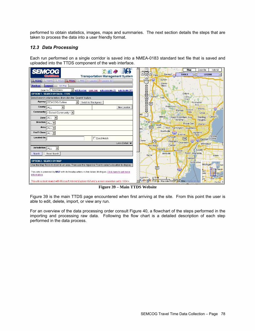
SEMCOG Travel Time Data Collection – Page 78
performed to obtain statistics, images, maps and summaries. The next section details the steps that are taken to process the data into a user friendly format.
12.3 Data Processing Each run performed on a single corridor is saved into a NMEA-0183 standard text file that is saved and uploaded into the TTDS component of the web interface.
Figure 39 – Main TTDS Website Figure 39 is the main TTDS page encountered when first arriving at the site. From this point the user is able to edit, delete, import, or view any run. For an overview of the data processing order consult Figure 40, a flowchart of the steps performed in the importing and processing raw data. Following the flow chart is a detailed description of each step performed in the data process.
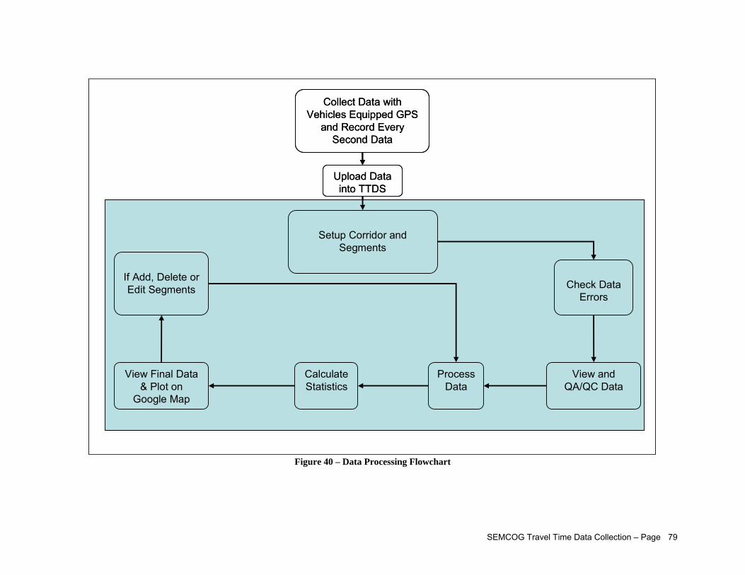
SEMCOG Travel Time Data Collection – Page 79
Setup Corridor and Segments
Collect Data with Vehicles Equipped GPS
and Record Every Second Data
View and QA/QC Data
Upload Data into TTDS
Check Data Errors
Process Data
Calculate Statistics
View Final Data & Plot on
Google Map
If Add, Delete or Edit Segments
Setup Corridor and Segments
Collect Data with Vehicles Equipped GPS
and Record Every Second Data
View and QA/QC Data
Upload Data into TTDS
Check Data Errors
Process Data
Calculate Statistics
View Final Data & Plot on
Google Map
If Add, Delete or Edit Segments
Figure 40 – Data Processing Flowchart
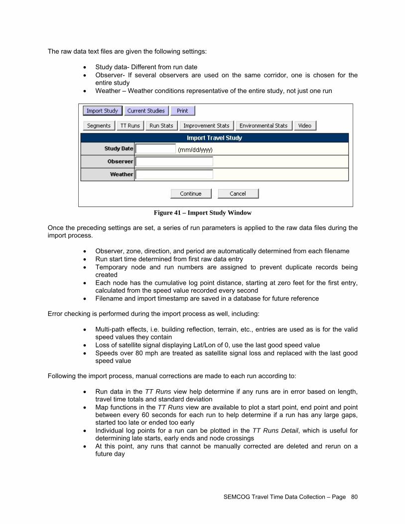
SEMCOG Travel Time Data Collection – Page 80
The raw data text files are given the following settings:
• Study data- Different from run date • Observer- If several observers are used on the same corridor, one is chosen for the
entire study • Weather – Weather conditions representative of the entire study, not just one run
Figure 41 – Import Study Window Once the preceding settings are set, a series of run parameters is applied to the raw data files during the import process.
• Observer, zone, direction, and period are automatically determined from each filename • Run start time determined from first raw data entry • Temporary node and run numbers are assigned to prevent duplicate records being
created • Each node has the cumulative log point distance, starting at zero feet for the first entry,
calculated from the speed value recorded every second • Filename and import timestamp are saved in a database for future reference
Error checking is performed during the import process as well, including:
• Multi-path effects, i.e. building reflection, terrain, etc., entries are used as is for the valid speed values they contain
• Loss of satellite signal displaying Lat/Lon of 0, use the last good speed value • Speeds over 80 mph are treated as satellite signal loss and replaced with the last good
speed value Following the import process, manual corrections are made to each run according to:
• Run data in the TT Runs view help determine if any runs are in error based on length, travel time totals and standard deviation
• Map functions in the TT Runs view are available to plot a start point, end point and point between every 60 seconds for each run to help determine if a run has any large gaps, started too late or ended too early
• Individual log points for a run can be plotted in the TT Runs Detail, which is useful for determining late starts, early ends and node crossings
• At this point, any runs that cannot be manually corrected are deleted and rerun on a future day
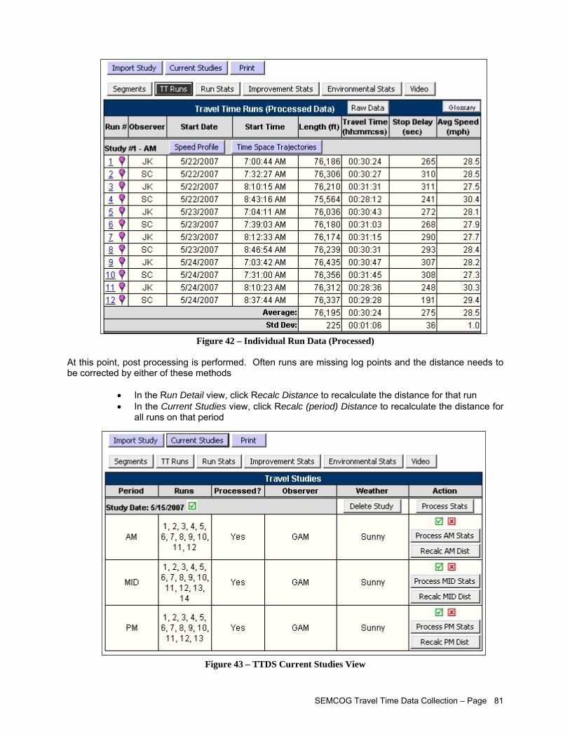
SEMCOG Travel Time Data Collection – Page 81
Figure 42 – Individual Run Data (Processed) At this point, post processing is performed. Often runs are missing log points and the distance needs to be corrected by either of these methods
• In the Run Detail view, click Recalc Distance to recalculate the distance for that run • In the Current Studies view, click Recalc (period) Distance to recalculate the distance for
all runs on that period
Figure 43 – TTDS Current Studies View
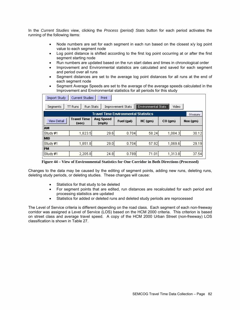
SEMCOG Travel Time Data Collection – Page 82
In the Current Studies view, clicking the Process (period) Stats button for each period activates the running of the following items:
• Node numbers are set for each segment in each run based on the closest x/y log point value to each segment node
• Log point distance is shifted according to the first log point occurring at or after the first segment starting node
• Run numbers are updated based on the run start dates and times in chronological order • Improvement and Environmental statistics are calculated and saved for each segment
and period over all runs • Segment distances are set to the average log point distances for all runs at the end of
each segment node • Segment Average Speeds are set to the average of the average speeds calculated in the
Improvement and Environmental statistics for all periods for this study
Figure 44 – View of Environmental Statistics for One Corridor in Both Directions (Processed) Changes to the data may be caused by the editing of segment points, adding new runs, deleting runs, deleting study periods, or deleting studies. These changes will cause:
• Statistics for that study to be deleted • For segment points that are edited, run distances are recalculated for each period and
processing statistics are updated • Statistics for added or deleted runs and deleted study periods are reprocessed
The Level of Service criteria is different depending on the road class. Each segment of each non-freeway corridor was assigned a Level of Service (LOS) based on the HCM 2000 criteria. This criterion is based on street class and average travel speed. A copy of the HCM 2000 Urban Street (non-freeway) LOS classification is shown in Table 27.
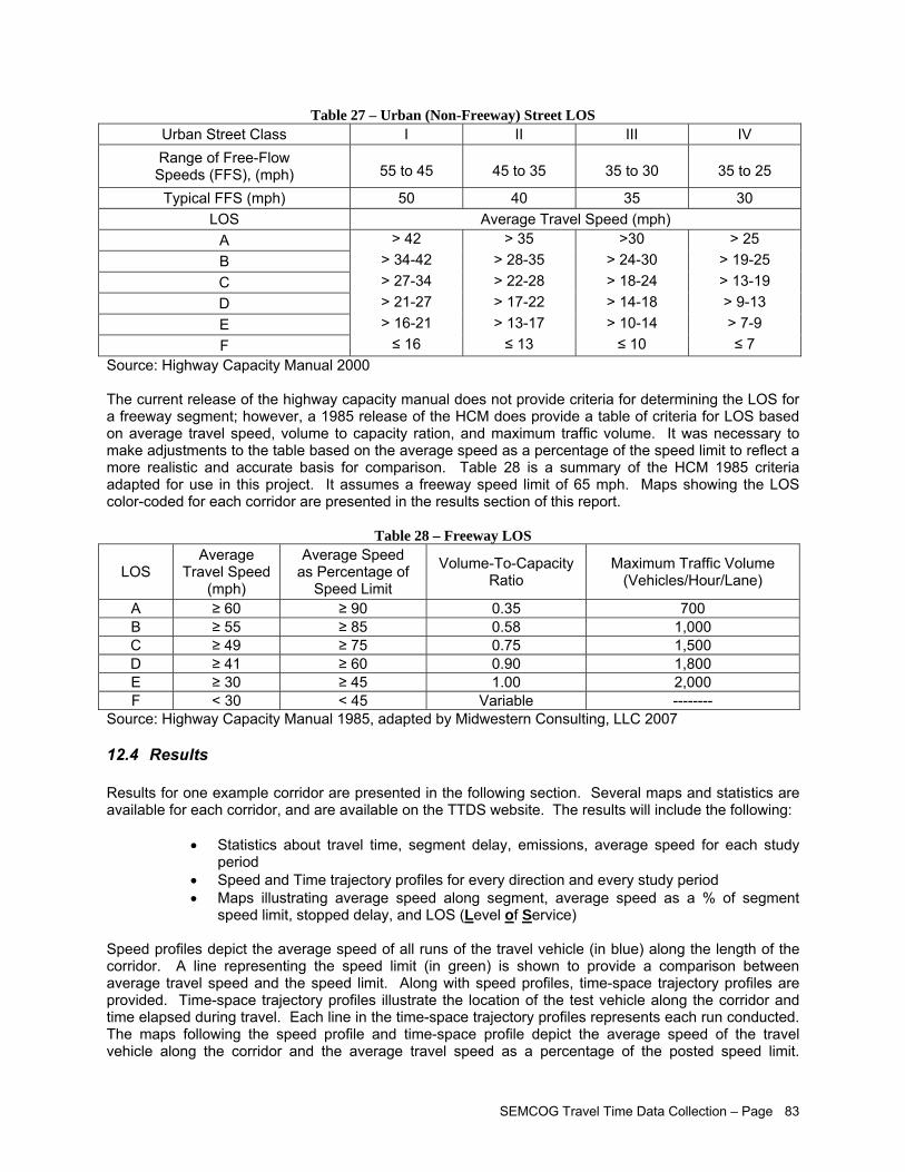
SEMCOG Travel Time Data Collection – Page 83
Table 27 – Urban (Non-Freeway) Street LOS Urban Street Class I II III IV Range of Free-Flow Speeds (FFS), (mph)
55 to 45
45 to 35
35 to 30
35 to 25
Typical FFS (mph) 50 40 35 30 LOS Average Travel Speed (mph)
A > 42 > 35 >30 > 25 B > 34-42 > 28-35 > 24-30 > 19-25 C > 27-34 > 22-28 > 18-24 > 13-19 D > 21-27 > 17-22 > 14-18 > 9-13 E > 16-21 > 13-17 > 10-14 > 7-9 F ≤ 16 ≤ 13 ≤ 10 ≤ 7
Source: Highway Capacity Manual 2000 The current release of the highway capacity manual does not provide criteria for determining the LOS for a freeway segment; however, a 1985 release of the HCM does provide a table of criteria for LOS based on average travel speed, volume to capacity ration, and maximum traffic volume. It was necessary to make adjustments to the table based on the average speed as a percentage of the speed limit to reflect a more realistic and accurate basis for comparison. Table 28 is a summary of the HCM 1985 criteria adapted for use in this project. It assumes a freeway speed limit of 65 mph. Maps showing the LOS color-coded for each corridor are presented in the results section of this report.
Table 28 – Freeway LOS
LOS Average
Travel Speed (mph)
Average Speed as Percentage of
Speed Limit
Volume-To-Capacity Ratio
Maximum Traffic Volume (Vehicles/Hour/Lane)
A ≥ 60 ≥ 90 0.35 700 B ≥ 55 ≥ 85 0.58 1,000 C ≥ 49 ≥ 75 0.75 1,500 D ≥ 41 ≥ 60 0.90 1,800 E ≥ 30 ≥ 45 1.00 2,000 F < 30 < 45 Variable --------
Source: Highway Capacity Manual 1985, adapted by Midwestern Consulting, LLC 2007
12.4 Results Results for one example corridor are presented in the following section. Several maps and statistics are available for each corridor, and are available on the TTDS website. The results will include the following:
• Statistics about travel time, segment delay, emissions, average speed for each study period
• Speed and Time trajectory profiles for every direction and every study period • Maps illustrating average speed along segment, average speed as a % of segment
speed limit, stopped delay, and LOS (Level of Service) Speed profiles depict the average speed of all runs of the travel vehicle (in blue) along the length of the corridor. A line representing the speed limit (in green) is shown to provide a comparison between average travel speed and the speed limit. Along with speed profiles, time-space trajectory profiles are provided. Time-space trajectory profiles illustrate the location of the test vehicle along the corridor and time elapsed during travel. Each line in the time-space trajectory profiles represents each run conducted. The maps following the speed profile and time-space profile depict the average speed of the travel vehicle along the corridor and the average travel speed as a percentage of the posted speed limit.
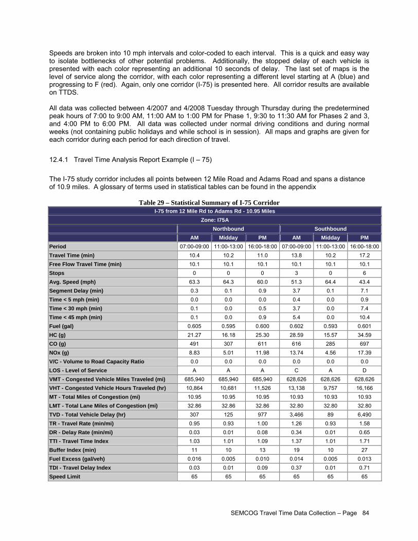
SEMCOG Travel Time Data Collection – Page 84
Speeds are broken into 10 mph intervals and color-coded to each interval. This is a quick and easy way to isolate bottlenecks of other potential problems. Additionally, the stopped delay of each vehicle is presented with each color representing an additional 10 seconds of delay. The last set of maps is the level of service along the corridor, with each color representing a different level starting at A (blue) and progressing to F (red). Again, only one corridor (I-75) is presented here. All corridor results are available on TTDS. All data was collected between 4/2007 and 4/2008 Tuesday through Thursday during the predetermined peak hours of 7:00 to 9:00 AM, 11:00 AM to 1:00 PM for Phase 1, 9:30 to 11:30 AM for Phases 2 and 3, and 4:00 PM to 6:00 PM. All data was collected under normal driving conditions and during normal weeks (not containing public holidays and while school is in session). All maps and graphs are given for each corridor during each period for each direction of travel.
12.4.1 Travel Time Analysis Report Example (I – 75) The I-75 study corridor includes all points between 12 Mile Road and Adams Road and spans a distance of 10.9 miles. A glossary of terms used in statistical tables can be found in the appendix
Table 29 – Statistical Summary of I-75 Corridor I-75 from 12 Mile Rd to Adams Rd - 10.95 Miles
Zone: I75A Northbound Southbound AM Midday PM AM Midday PM
Period 07:00-09:00 11:00-13:00 16:00-18:00 07:00-09:00 11:00-13:00 16:00-18:00Travel Time (min) 10.4 10.2 11.0 13.8 10.2 17.2 Free Flow Travel Time (min) 10.1 10.1 10.1 10.1 10.1 10.1 Stops 0 0 0 3 0 6 Avg. Speed (mph) 63.3 64.3 60.0 51.3 64.4 43.4 Segment Delay (min) 0.3 0.1 0.9 3.7 0.1 7.1 Time < 5 mph (min) 0.0 0.0 0.0 0.4 0.0 0.9 Time < 30 mph (min) 0.1 0.0 0.5 3.7 0.0 7.4 Time < 45 mph (min) 0.1 0.0 0.9 5.4 0.0 10.4 Fuel (gal) 0.605 0.595 0.600 0.602 0.593 0.601 HC (g) 21.27 16.18 25.30 28.59 15.57 34.59 CO (g) 491 307 611 616 285 697 NOx (g) 8.83 5.01 11.98 13.74 4.56 17.39 V/C - Volume to Road Capacity Ratio 0.0 0.0 0.0 0.0 0.0 0.0 LOS - Level of Service A A A C A D VMT - Congested Vehicle Miles Traveled (mi) 685,940 685,940 685,940 628,626 628,626 628,626 VHT - Congested Vehicle Hours Traveled (hr) 10,864 10,681 11,526 13,138 9,757 16,166 MT - Total Miles of Congestion (mi) 10.95 10.95 10.95 10.93 10.93 10.93 LMT - Total Lane Miles of Congestion (mi) 32.86 32.86 32.86 32.80 32.80 32.80 TVD - Total Vehicle Delay (hr) 307 125 977 3,466 89 6,490 TR - Travel Rate (min/mi) 0.95 0.93 1.00 1.26 0.93 1.58 DR - Delay Rate (min/mi) 0.03 0.01 0.08 0.34 0.01 0.65 TTI - Travel Time Index 1.03 1.01 1.09 1.37 1.01 1.71 Buffer Index (min) 11 10 13 19 10 27 Fuel Excess (gal/veh) 0.016 0.005 0.010 0.014 0.005 0.013 TDI - Travel Delay Index 0.03 0.01 0.09 0.37 0.01 0.71 Speed Limit 65 65 65 65 65 65
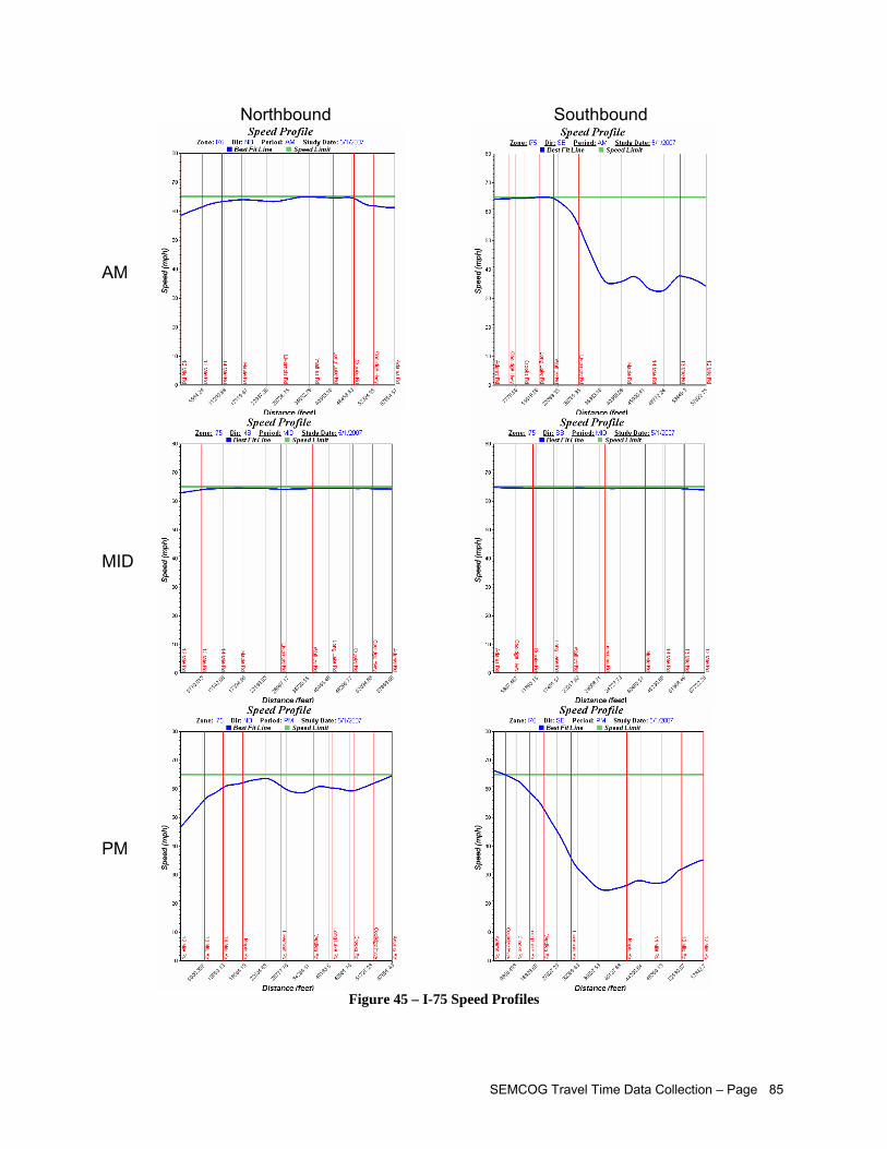
SEMCOG Travel Time Data Collection – Page 85
Northbound Southbound
Figure 45 – I-75 Speed Profiles
AM
MID
PM
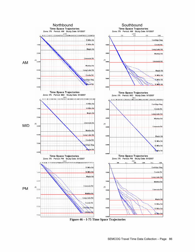
SEMCOG Travel Time Data Collection – Page 86
Northbound Southbound
Figure 46 – I-75 Time Space Trajectories
AM
MID
PM
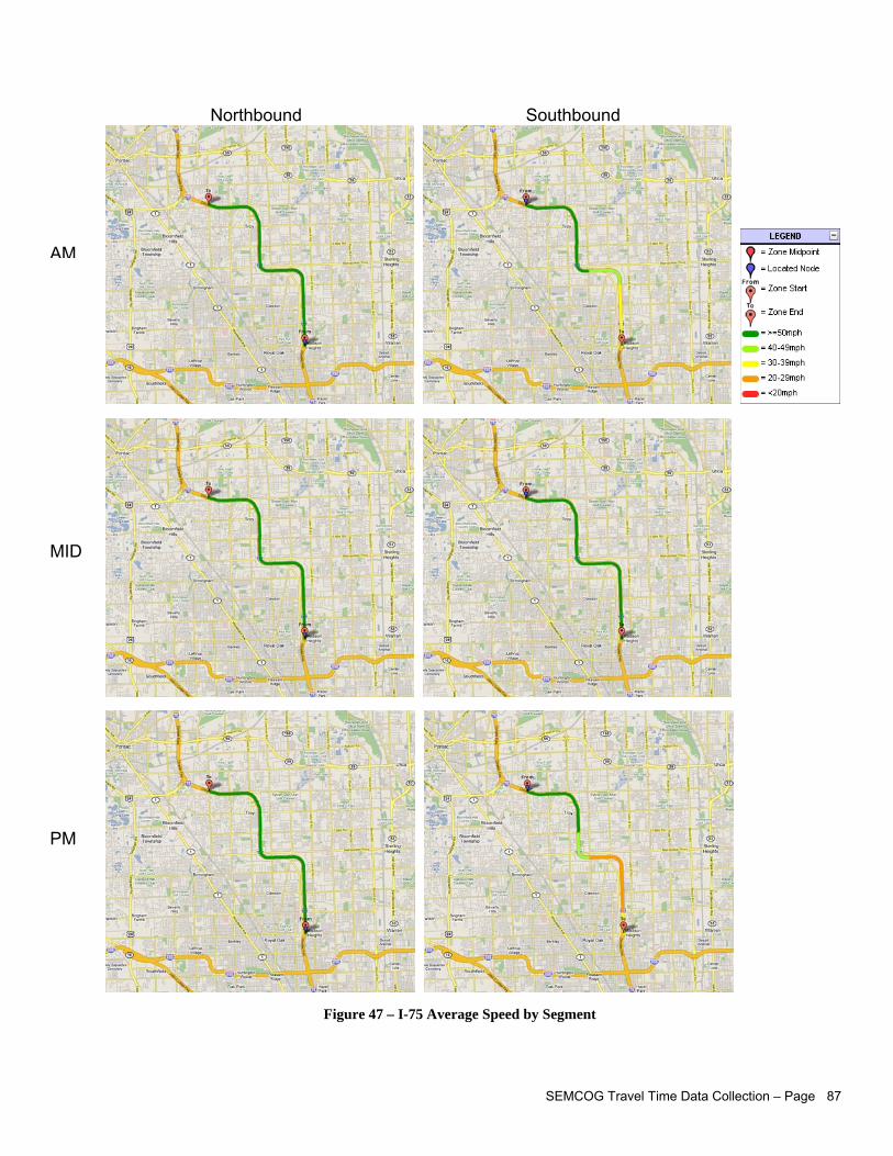
SEMCOG Travel Time Data Collection – Page 87
Northbound Southbound
Figure 47 – I-75 Average Speed by Segment
AM
MID
PM
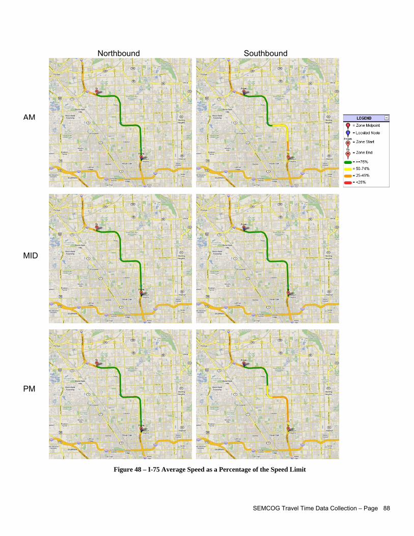
SEMCOG Travel Time Data Collection – Page 88
Northbound Southbound
Figure 48 – I-75 Average Speed as a Percentage of the Speed Limit
AM
MID
PM
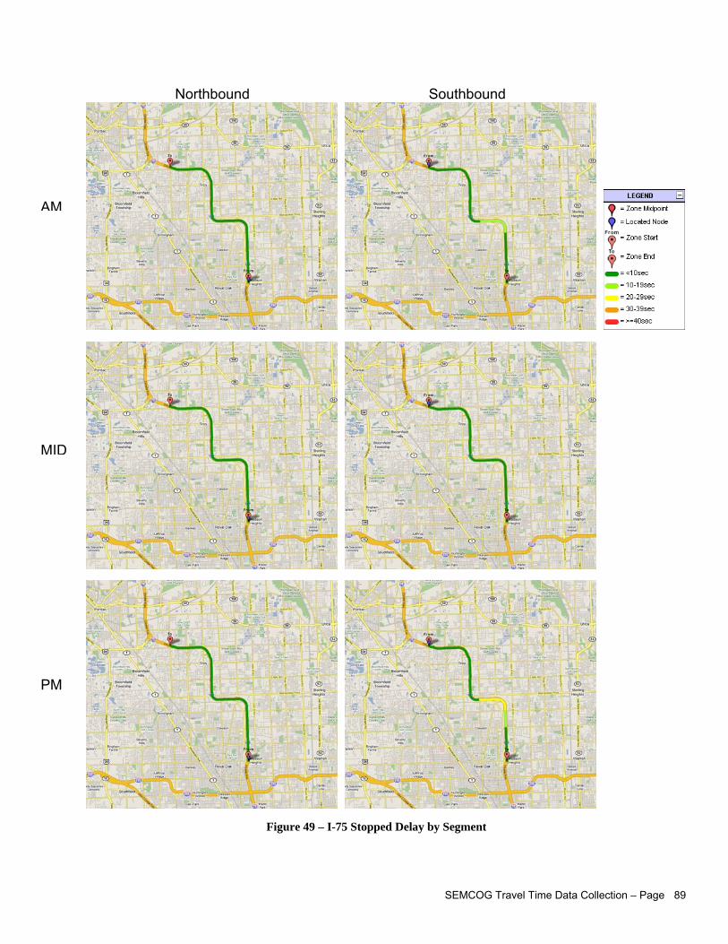
SEMCOG Travel Time Data Collection – Page 89
Northbound Southbound
Figure 49 – I-75 Stopped Delay by Segment
AM
MID
PM
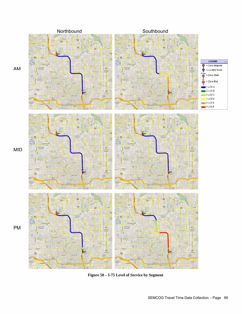
SEMCOG Travel Time Data Collection – Page 90
Northbound Southbound
Figure 50 – I-75 Level of Service by Segment
AM
MID
PM
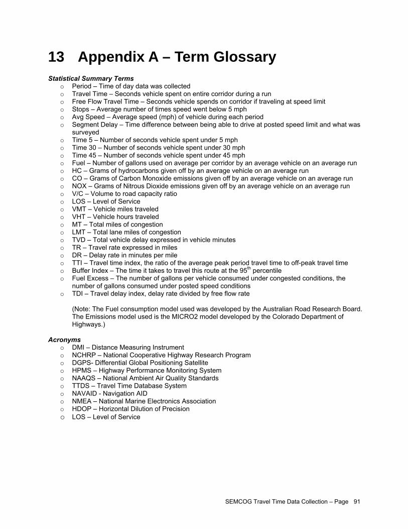
SEMCOG Travel Time Data Collection – Page 91
13 Appendix A – Term Glossary Statistical Summary Terms
o Period – Time of day data was collected o Travel Time – Seconds vehicle spent on entire corridor during a run o Free Flow Travel Time – Seconds vehicle spends on corridor if traveling at speed limit o Stops – Average number of times speed went below 5 mph o Avg Speed – Average speed (mph) of vehicle during each period o Segment Delay – Time difference between being able to drive at posted speed limit and what was
surveyed o Time 5 – Number of seconds vehicle spent under 5 mph o Time 30 – Number of seconds vehicle spent under 30 mph o Time 45 – Number of seconds vehicle spent under 45 mph o Fuel – Number of gallons used on average per corridor by an average vehicle on an average run o HC – Grams of hydrocarbons given off by an average vehicle on an average run o CO – Grams of Carbon Monoxide emissions given off by an average vehicle on an average run o NOX – Grams of Nitrous Dioxide emissions given off by an average vehicle on an average run o V/C – Volume to road capacity ratio o LOS – Level of Service o VMT – Vehicle miles traveled o VHT – Vehicle hours traveled o MT – Total miles of congestion o LMT – Total lane miles of congestion o TVD – Total vehicle delay expressed in vehicle minutes o TR – Travel rate expressed in miles o DR – Delay rate in minutes per mile o TTI – Travel time index, the ratio of the average peak period travel time to off-peak travel time o Buffer Index – The time it takes to travel this route at the 95th percentile o Fuel Excess – The number of gallons per vehicle consumed under congested conditions, the
number of gallons consumed under posted speed conditions o TDI – Travel delay index, delay rate divided by free flow rate
(Note: The Fuel consumption model used was developed by the Australian Road Research Board. The Emissions model used is the MICRO2 model developed by the Colorado Department of Highways.)
Acronyms
o DMI – Distance Measuring Instrument o NCHRP – National Cooperative Highway Research Program o DGPS- Differential Global Positioning Satellite o HPMS – Highway Performance Monitoring System o NAAQS – National Ambient Air Quality Standards o TTDS – Travel Time Database System o NAVAID - Navigation AID o NMEA – National Marine Electronics Association o HDOP – Horizontal Dilution of Precision o LOS – Level of Service
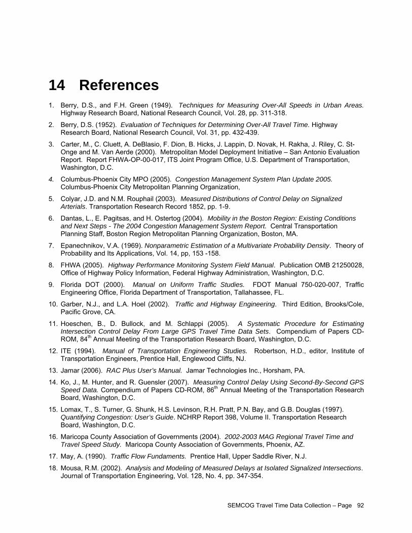
SEMCOG Travel Time Data Collection – Page 92
14 References 1. Berry, D.S., and F.H. Green (1949). Techniques for Measuring Over-All Speeds in Urban Areas.
Highway Research Board, National Research Council, Vol. 28, pp. 311-318.
2. Berry, D.S. (1952). Evaluation of Techniques for Determining Over-All Travel Time. Highway Research Board, National Research Council, Vol. 31, pp. 432-439.
3. Carter, M., C. Cluett, A. DeBlasio, F. Dion, B. Hicks, J. Lappin, D. Novak, H. Rakha, J. Riley, C. St-Onge and M. Van Aerde (2000). Metropolitan Model Deployment Initiative – San Antonio Evaluation Report. Report FHWA-OP-00-017, ITS Joint Program Office, U.S. Department of Transportation, Washington, D.C.
4. Columbus-Phoenix City MPO (2005). Congestion Management System Plan Update 2005. Columbus-Phoenix City Metropolitan Planning Organization,
5. Colyar, J.D. and N.M. Rouphail (2003). Measured Distributions of Control Delay on Signalized Arterials. Transportation Research Record 1852, pp. 1-9.
6. Dantas, L., E. Pagitsas, and H. Ostertog (2004). Mobility in the Boston Region: Existing Conditions and Next Steps - The 2004 Congestion Management System Report. Central Transportation Planning Staff, Boston Region Metropolitan Planning Organization, Boston, MA.
7. Epanechnikov, V.A. (1969). Nonparametric Estimation of a Multivariate Probability Density. Theory of Probability and Its Applications, Vol. 14, pp, 153 -158.
8. FHWA (2005). Highway Performance Monitoring System Field Manual. Publication OMB 21250028, Office of Highway Policy Information, Federal Highway Administration, Washington, D.C.
9. Florida DOT (2000). Manual on Uniform Traffic Studies. FDOT Manual 750-020-007, Traffic Engineering Office, Florida Department of Transportation, Tallahassee, FL.
10. Garber, N.J., and L.A. Hoel (2002). Traffic and Highway Engineering. Third Edition, Brooks/Cole, Pacific Grove, CA.
11. Hoeschen, B., D. Bullock, and M. Schlappi (2005). A Systematic Procedure for Estimating Intersection Control Delay From Large GPS Travel Time Data Sets. Compendium of Papers CD-ROM, 84th Annual Meeting of the Transportation Research Board, Washington, D.C.
12. ITE (1994). Manual of Transportation Engineering Studies. Robertson, H.D., editor, Institute of Transportation Engineers, Prentice Hall, Englewood Cliffs, NJ.
13. Jamar (2006). RAC Plus User’s Manual. Jamar Technologies Inc., Horsham, PA.
14. Ko, J., M. Hunter, and R. Guensler (2007). Measuring Control Delay Using Second-By-Second GPS Speed Data. Compendium of Papers CD-ROM, 86th Annual Meeting of the Transportation Research Board, Washington, D.C.
15. Lomax, T., S. Turner, G. Shunk, H.S. Levinson, R.H. Pratt, P.N. Bay, and G.B. Douglas (1997). Quantifying Congestion: User’s Guide. NCHRP Report 398, Volume II. Transportation Research Board, Washington, D.C.
16. Maricopa County Association of Governments (2004). 2002-2003 MAG Regional Travel Time and Travel Speed Study. Maricopa County Association of Governments, Phoenix, AZ.
17. May, A. (1990). Traffic Flow Fundaments. Prentice Hall, Upper Saddle River, N.J.
18. Mousa, R.M. (2002). Analysis and Modeling of Measured Delays at Isolated Signalized Intersections. Journal of Transportation Engineering, Vol. 128, No. 4, pp. 347-354.
SEMCOG Travel Time Data Collection – Page 93
19. National Committee on Urban Transportation (1953). Better Transportation for Your City: A Guide for the Factual Development of Urban Transportation Plans. Procedural Manual 3B, National Committee on Urban Transportation, Public Administration Service, Chicago, Illinois.
20. Oppenlander, J.C. (1976). Sample Size Determination for Travel Time and Delay Studies. Traffic Engineering, September 1976, pp. 25-28.
21. Overton, R. (2007). Travel Time Delay Study Procedure Manual. Data Collection Section, Asset Management Division, Bureau of Transportation Planning, Michigan Department of Transportation, Lansing, MI.
22. Quiroga, C.A., and D. Bullock (1998a). Determination of Travel Sample Sizes for Travel Time Studies. ITE Journal on the Web, August 1998, pp. 92-98.
23. Quiroga, C. and D. Bullock (1998b). Travel Time Studies with Global Positioning and Geographic Information Systems: An Integrated Methodology. Transportation Research Part C, Vol. 6C, No. 1/2, pp. 101-127.
24. Quiroga, C. and D. Bullock (1999). Measuring Control Delay at Signalized Intersections. Journal of Transportation Engineering, Vol. 125, No. 4, pp. 271-280.
25. Rakha, H., F. Dion and H.-G. Sin (2001). Using Global Positioning System Data for Field Evaluation of Energy and Emission Impact of Traffic Flow Improvement Projects. Transportation Record 1768, pp. 211-223.
26. Schrank, D., and T. Lomax (2005). The 2005 Urban Mobility Report. Texas Transportation Institute, The Texas A&M University System, College Station, TX.
27. TTI (2004). Methodology for 2004 Annual Report. Texas Transportation Institute. College Station, TX. Retrieved from http://mobility.tamu.edu/ums/report/methodology.stm on July 11, 2007.
28. TRB (2000). Highway Capacity Manual. Transportation Research Board Washington D.C.
29. Turner, S.M., W.L. Eisele, R.J. Benz, and D.J. Holdener (1998). The Travel Time Data Collection Handbook. Texas Transportation Institute, Federal Highway Administration Report No. FHWA-PL-98-035.