T

TANGANYIKA LAKE, MODELING THEECO-HYDRODYNAMICS

Jaya Naithani1, Pierre-Denis Plisnier2, Eric Deleersnijder11G. Lemaître Centre for Earth and Climate Research(TECLIM), Institute of Mechanics, Materials and CivilEngineering (iMMC), Université catholique de Louvain,Earth and Life Institute (ELI), Louvain-la-Neuve,Belgium2Royal Museum for Central Africa, Tervuren, Belgium

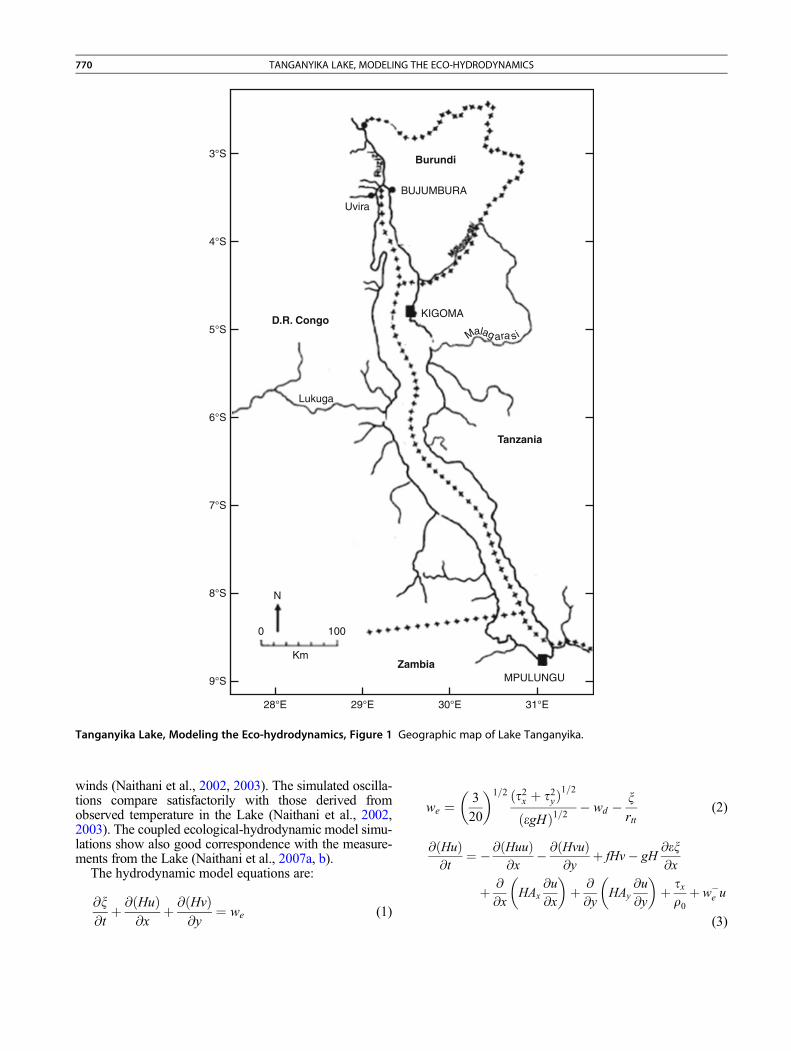
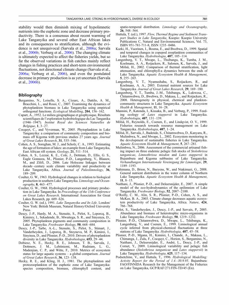
IntroductionLake Tanganyika is one of the Great Rift Valley Lakesof East Africa (Figure 1) and is situated between 3�Sand 9�S. It is 650 km long with a mean width of around50 km and an average depth of 570 m. It is a freshwaterLake characterized by a quasi-permanent thermocline.The Lake is meromictic – complete overturning of thewater never takes place – and mixing occurs only par-tially. The epilimnion (surface layer) undergoes sea-sonal temperature change annually, while thehypolimnion is anoxic with an invariant temperature.The hypolimnion is a vast reservoir of nutrients largelyisolated from surface influences (Hecky and Fee, 1981;Hecky et al., 1991). The average transparency of theLake is close to 11 m. The solar radiation around theLake varies very little in the year because of its closerproximity to the equator. The nutrients supplied to themixed layer, where photosynthesis can occur, aremainly internal nutrients from within the Lake, whereasriverine and atmospheric input of nutrients is consid-ered negligible for Lake Tanganyika (Hecky and Fee,1981; Sarvala et al., 1999a; Langenberg et al., 2003a).Nutrients from the hypolimnion are supplied to the epi-limnion mainly by wind-driven upwelling of the strongsoutheast winds during the dry season from March/April

L. Bengtsson, R.W. Herschy, R.W. Fairbridge (eds.), Encyclopedia of Lakes and R# Springer Science+Business Media B.V. 2012

until August/September (Hecky et al., 1991;Plisnier et al., 1999; Langenberg et al., 2003b). The windstress pushes the warmer surface water away from thesouthern end of the Lake toward the northern end,resulting in a well-known compensating upwelling in thesouth. This upwelling results in the seasonal enhancementof the nutrients in the euphotic layer initiating phytoplank-ton blooms. Apart from this major wind-induced southernupwelling, small coastal upwellings can also be seen fromtime to time propagating clockwise around the westernboundaries of the lake, which are the internal Kelvin wavepackets (Naithani and Deleersnijder, 2004). During the wetseason, the primary production is less important and is pri-marily dependent on the nutrients regenerated within theepilimnion (Coulter and Spigel, 1991).

The above mentioned thermodynamic, hydrodynamic,and ecological characteristics are incorporated into aneco-hydrodynamic model to study the primary food webof Lake Tanganyika. The hydrodynamic model comprisesnonlinear, reduced-gravity equations (Naithani et al.,2002, 2003). The ecological model components includeone nutrient, phytoplankton biomass, zooplankton bio-mass, and detritus (Naithani et al., 2007a, b, 2011).

Materials and methodThe model consists of a four-component ecosystem model,coupled to a hydrodynamic model. The hydrodynamicmodel considers the Lake as two homogeneous layers ofdifferent density lying above each other, representing thewarm epilimnion (surface mixed layer) and cold densehypolimnion (lower layer) separated by a thermocline(Naithani et al., 2002, 2003). The lower layer is consideredto be much deeper than the surface active/mixed layer. Themodel is forced with the wind and solar radiation data fromthe NCEP reanalysis. Studies using the hydrodynamicmodel have shown that in the motion of water there areinternal waves with oscillations similar to that in the forcing

eservoirs, DOI 10.1007/978-1-4020-4410-6,

28°E

9°S

8°S

7°S

6°S

5°S

4°S

BUJUMBURA

Uvira

KIGOMA

Lukuga

3°S

29°E

Km

N

1000

Zambia

Tanzania

D.R. Congo

Burundi

30°E

MPULUNGU

31°E

Malag ara si

Tanganyika Lake, Modeling the Eco-hydrodynamics, Figure 1 Geographic map of Lake Tanganyika.

770 TANGANYIKA LAKE, MODELING THE ECO-HYDRODYNAMICS

winds (Naithani et al., 2002, 2003). The simulated oscilla-tions compare satisfactorily with those derived fromobserved temperature in the Lake (Naithani et al., 2002,2003). The coupled ecological-hydrodynamic model simu-lations show also good correspondence with the measure-ments from the Lake (Naithani et al., 2007a, b).

The hydrodynamic model equations are:

@x@t

þ @ðHuÞ@x

þ @ðHvÞ@y

¼ we (1)

� �1=2 2 2 1=2

we ¼ 320

ðtx þ tyÞðegHÞ1=2

� wd � xrtt

(2)

@ðHuÞ @ðHuuÞ @ðHvuÞ @ex

@t

¼ �@x

�@y

þ fHv� gH@x

þ @

@xHAx

@u@x

� �þ @

@yHAy

@u@y

� �þ txr0

þ w�e u

(3)

TANGANYIKA LAKE, MODELING THE ECO-HYDRODYNAMICS 771

@ðHvÞ @ðHuvÞ @ðHvvÞ @ex

@t

¼ �@x

�@y

� fHu� gH@y

þ @

@xHAx

@v@x

� �þ @

@yHAy

@v@y

� �þ tyr0

þ w�e v

(4)

where x and y are horizontal axes, u and v are the depth-integrated velocity components in the surface layer inthe x and y directions, t is the time, x is the downward dis-placement of the thermocline, H ¼ hþ x is the thicknessof the epilimnion (the surface, well-mixed layer), h is thereference depth of the surface layer (m), and we is theentrainment velocity (ms�1). The first term on the righthand side of Equation 2 is inspired by Price (1979), txand ty are horizontal components of specific wind stressin the x and y direction (m2s�2), and e ¼ ðrb � rsÞ=rb isthe relative density difference between the hypolimnion(rb) and the epilimnion (rs), calculated using the temper-ature of the surface layer (ts) and bottom layer (tb) respec-tively. wd is the detrainment term (ms�1), defined suchthat the annual mean of the epilimnion volume remainsapproximately constant. There are large uncertainties inthe parameterization of entrainment and detrainmentterms. As a consequence, to avoid occasional spuriousvalues of x, a relaxation term (x/rtt) is needed whichslowly nudges the surface layer depth toward its equilib-rium position. The relaxation timescale, rtt, is sufficientlylong so that the relaxation term is generally smaller thanthe entrainment and detrainment terms. f is the Coriolisfactor (<0 in the southern hemisphere), and As is the hor-izontal eddy viscosity in the s (=x,y) direction.

uptake

Phytoplanktoncopepgrazi

respiratoryrelease

solubleexcretion

diso

pho

beregen

Phosphate

epilimnion

z=0surface

z=H

hypolimnion

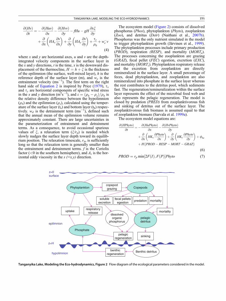
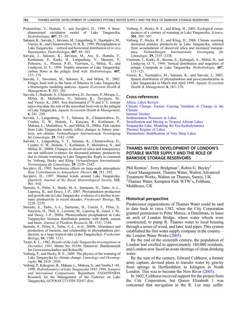
Tanganyika Lake, Modeling the Eco-hydrodynamics, Figure 2 Flo

The ecosystem model (Figure 2) consists of dissolvedphosphorus (Phos), phytoplankton (Phyto), zooplankton(Zoo), and detritus (Detr) (Naithani et al., 2007b).Phosphorus was the only nutrient simulated in the modelto trigger phytoplankton growth (Järvinen et al., 1999).The phytoplankton processes include primary production(PROD), respiration (RESP), and mortality (MORTa).The processes concerning the zooplankton are grazing(GRAZ), fecal pellet (FEC) egestion, excretion (EXC),and mortality (MORTz). Phytoplankton respiratory releaseand the excretion from zooplankton are directlyremineralized in the surface layer. A small percentage offeces, dead phytoplankton, and zooplankton are alsoremineralized into phosphate in the surface layer whereasthe rest contributes to the detritus pool, which sedimentsfast. The regeneration/remineralization within the surfacelayer represents the effect of the microbial food web andalso represents the pelagic regeneration. The model isclosed by predation (PRED) from zooplanktivorous fishand sinking of detritus out of the surface layer. Thezooplanktivorous fish biomass is assumed equal to thatof zooplankton biomass (Sarvala et al. 1999a).

The ecosystem model equations are:

@ðHPhytoÞ@t

¼� @ðHuPhytoÞ@x

� @ðHvPhytoÞ@y

þ @

@xHKx

@Phyto@x

� �þ @

@yHKy

@Phyto@y

� �þ fhe

þ H PROD� RESP �MORT � GRAZf g(6)

PROD ¼ rp min 2FðIÞ;FðPÞ½ �Phyto (7)

odng Copepods

fecal pelletsegestion

predation mortality

mortality

pelagicdetritus

sinking

solvedrganicsphorus

pelagicregeneration

nthiceration

Benthic detritus

wdiagram of the ecological parameters considered in themodel.

772 TANGANYIKA LAKE, MODELING THE ECO-HYDRODYNAMICS

RESP ¼ rarp min 2FðIÞ;FðPÞ½ �Phyto (8)

MORTa ¼ maPhyto (9)

Phyto

GRAZ ¼ rz Phytoþ kphyto

Zoo (10)

Phos

FðPÞ ¼

Phosþ kphos(11)

FðIÞ ¼ ð1=k HÞ½arctanðaI =2I Þ � arctanðaI e�keH=2:IkÞÞ�

e 0 k 0

(12)

Phyto

ke ¼ 0:066þ 0:07

rc(13)

f ¼ wþPhyto þ w�Phyto (14)

he e h e

@ðHZooÞ @ðHuZooÞ @ðHvZooÞ

@t

¼�@x

�@y

þ @

@xHKx

@Zoo

@x

� �þ @

@yHKy

@Zoo

@y

� �þ fhe

þ H GRAZ � EXC � FEC �MORTz � PREDf g(15)

EXC ¼ neGRAZ (16)

FEC ¼ nf GRAZ (17)

MORTz ¼ mzGRAZ (18)

Zoo

PRED ¼ rf Zooþ kzoo

Fish (19)

@ðHPhosÞ @ðHuPhosÞ @ðHvPhosÞ

@t

¼�@x

�@y

þ @

@xHKx

@Phos@x

� �þ @

@yHKy

@Phos@y

� �

þ fhe þ H�ðPROD� RESPÞ

CPaþ paMORTa

CPa

(

þ ðpf FEC þ pzMORTz þ EXCÞCPz

!)

(20)

@ðHDetrÞ @ðHuDetrÞ @ðHvDetrÞ

@t

¼�@x

�@y

þ @

@xHKx

@Detr

@x

� �þ @

@yHKy

@Detr

@y

� �þ fhe

þ Hfð1� mpÞMORTa þ ð1� pf ÞFECþ ð1� pzÞMORTz � rdDetrg � wdDetr

(21)

The first four terms on the right hand side of Equations 6,

15, 20, and 21 represent the horizontal advection anddiffusion of the ecological parameters, u and v aretime-dependent horizontal velocities obtained from thecirculation model, and Kx and Ky are the horizontal

diffusion coefficients. The fifth term represents entrain-ment from hypolimnion. Entrainment of phosphate fromthe hypolimnion was extrapolated exponentially from45 mgPL�1 below 60m depth to 1 mgPL�1 near the surface(Coulter and Spigel, 1991; Plisnier et al., 1996; Plisnierand Descy, 2005). This ensured that the water is richer innutrients if upwelling occurs from deeper depths. The def-inition of the parameters and their values are given inTable 1. Model was run with the thermocline at 30 mand the temperature of the surface and lower layers as27�C and 24.5�C, respectively for the years 2002–2009.

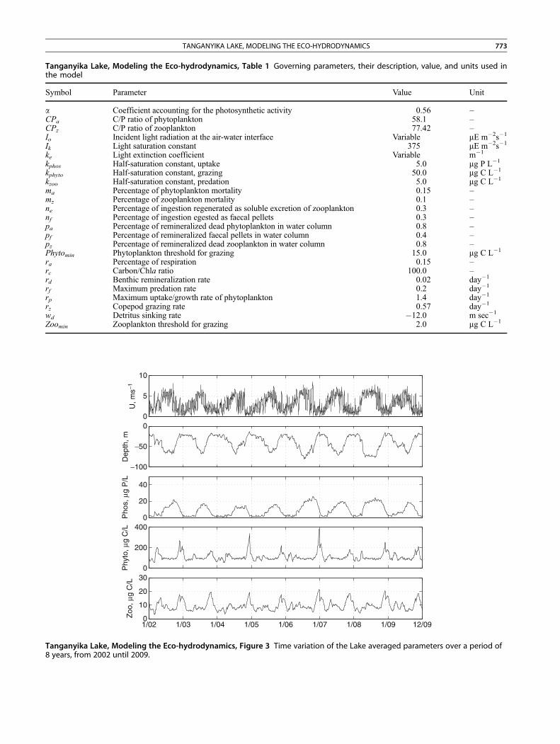
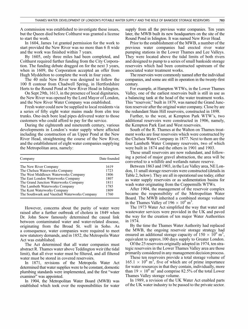
Results and discussionFigure 3 shows the time series of wind speed, modelpredicted surface layer (epilimnion) depth, and thedepth-averaged concentration in the surface layer of phos-phate, phytoplankton biomass, and zooplankton biomass.The surface layer depth increases at the beginning of thedry season because of wind driven mixing and remainsat greater depth during the whole season. It decreases atthe end of the dry season and remains more or less at thisdepth during the wet season until the beginning of the nextdry season. Phosphate concentration closely follows themixed layer depth. It increases because of entrainmentassociated to the upwelling of nutrients from below andremains high for the rest of the dry season, because ofalmost continuous upwelling, and decreases at the end ofthe dry season. Increase in the biomass of phytoplanktonat the beginning of the dry season is natural because ofthe input of nutrients in the surface layer. However, thephytoplankton biomass cannot sustain at this high valueand decreases in spite of the continuous abundance ofnutrients. The increased surface layer depth caused by per-sistently higher winds forced the algal community tospend more time in deeper water with reduced light,thereby decreasing the productivity. Phytoplankton bio-mass shows another bloom at the end of the dry seasonwhen the SE wind diminishes and, subsequently, changesdirection, and the surface layer still carrying adequateamounts of nutrients relaxes back to shallower depths(Plisnier et al., 1999). Phytoplankton biomass in effectshowed a trade-off between the availability of nutrientsand light. Negative effects of deep mixing on the phyto-plankton biomass were also considered by Sarvala et al.(1999b).

Effect of changing the model ecological parametersIncreasing (decreasing) the half-saturation constant forgrazing decreased (increased) the zooplankton biomassand increased (decreased) phytoplankton biomass(Naithani et al., 2007a). The change in the phytoplanktonbiomass is almost half the change in the zooplankton bio-mass. Decreasing the predator population increases thezooplankton biomass and vice versa. For these tests withthe predator population the change in the phytoplanktonbiomass is much less than the change in the zooplanktonbiomass. It is seen that the primary production, which

0

5

10

U, m

s−1

−100

−50

0

Dep

th, m

0

20

40

Pho

s, µ

g P

/L

0

200

400

Phy

to, µ

g C

/L

1/02 1/03 1/04 1/05 1/06 1/07 1/08 1/09 12/090

10

20

30

Zoo

, µg

C/L

Tanganyika Lake, Modeling the Eco-hydrodynamics, Figure 3 Time variation of the Lake averaged parameters over a period of8 years, from 2002 until 2009.

Tanganyika Lake, Modeling the Eco-hydrodynamics, Table 1 Governing parameters, their description, value, and units used inthe model

Symbol Parameter Value Unit

a Coefficient accounting for the photosynthetic activity 0.56 –CPa C/P ratio of phytoplankton 58.1 –CPz C/P ratio of zooplankton 77.42 –Io Incident light radiation at the air-water interface Variable mE m�2s�1

Ik Light saturation constant 375 mE m�2s�1

ke Light extinction coefficient Variable m�1

kphos Half-saturation constant, uptake 5.0 mg P L�1

kphyto Half-saturation constant, grazing 50.0 mg C L�1

kzoo Half-saturation constant, predation 5.0 mg C L�1

ma Percentage of phytoplankton mortality 0.15 –mz Percentage of zooplankton mortality 0.1 –ne Percentage of ingestion regenerated as soluble excretion of zooplankton 0.3 –nf Percentage of ingestion egested as faecal pellets 0.3 –pa Percentage of remineralized dead phytoplankton in water column 0.8 –pf Percentage of remineralized faecal pellets in water column 0.4 –pz Percentage of remineralized dead zooplankton in water column 0.8 –Phytomin Phytoplankton threshold for grazing 15.0 mg C L�1

ra Percentage of respiration 0.15 –rc Carbon/Chla ratio 100.0 –rd Benthic remineralization rate 0.02 day�1

rf Maximum predation rate 0.2 day�1

rp Maximum uptake/growth rate of phytoplankton 1.4 day�1

rz Copepod grazing rate 0.57 day�1

wd Detritus sinking rate �12.0 m sec�1

Zoomin Zooplankton threshold for grazing 2.0 mg C L�1

TANGANYIKA LAKE, MODELING THE ECO-HYDRODYNAMICS 773

774 TANGANYIKA LAKE, MODELING THE ECO-HYDRODYNAMICS

strongly depends upon the light in the water column andentrainment of nutrients, is bottom-up controlled, whileit seems that predator abundance strongly controls zoo-plankton biomass (top-down control, Naithani et al.,2007a). By contrast, fish predation influence seemsreduced on the phytoplankton level. In other words, anychange in predator biomass significantly affects the herbi-vore biomass, but has little influence on phytoplanktonbiomass. Indeed, in our simulations, reduced grazing pres-sure from top-down control of mesozooplankton did notincrease phytoplankton abundance considerably. Inplanktivore-dominated Lake Tanganyika, zooplanktonare not able to control phytoplankton, and therefore, lightor nutrient limitation and resource competition seem to becommon among the latter (Järvinen et al., 1999).

ts, °C ts, °C

ts, °C ts, °C

ts, °C ts, °C

h, m

H, m

60 50

40

a1 25 26 27 28 29

20

30

40

50

6070

40

60

80

PHOS, µg P/L

35

25

2555

15

a2 25 26 27 28 29

20

40

60

Win

d st

ress

, m2

s−2 (h=30 m), H, m

6050

40

b1 25 26 27 28 29

*0.6

*0.8

*1.0

*1.2

*1.4

*1.640

60

80

(h=30 m), PHOS, µg P/L

50 25

30

15

b2 25 26 27 28 29

20

40

60

Win

d st

ress

, m2

s−2 (ts=27 °C), H, m

60

5040

c1 30 50 70

*0.6

*0.8

*1.0

*1.2

*1.4

*1.640

60

80

(ts=27 °C), PHOS, µg P/L

1535

25 50

c2 30 50 70

20

40

60

h, mh, m

Win

d st

ress

, m2

s−2 (h=70 m), H, m

60

d1 25 26 27 28 29

*0.6

*0.8

*1.0

*1.2

*1.4

*1.640

60

80

(h=70 m), PHOS, µg P/L

6040

20

25

d2 25 26 27 28 29

20

40

60

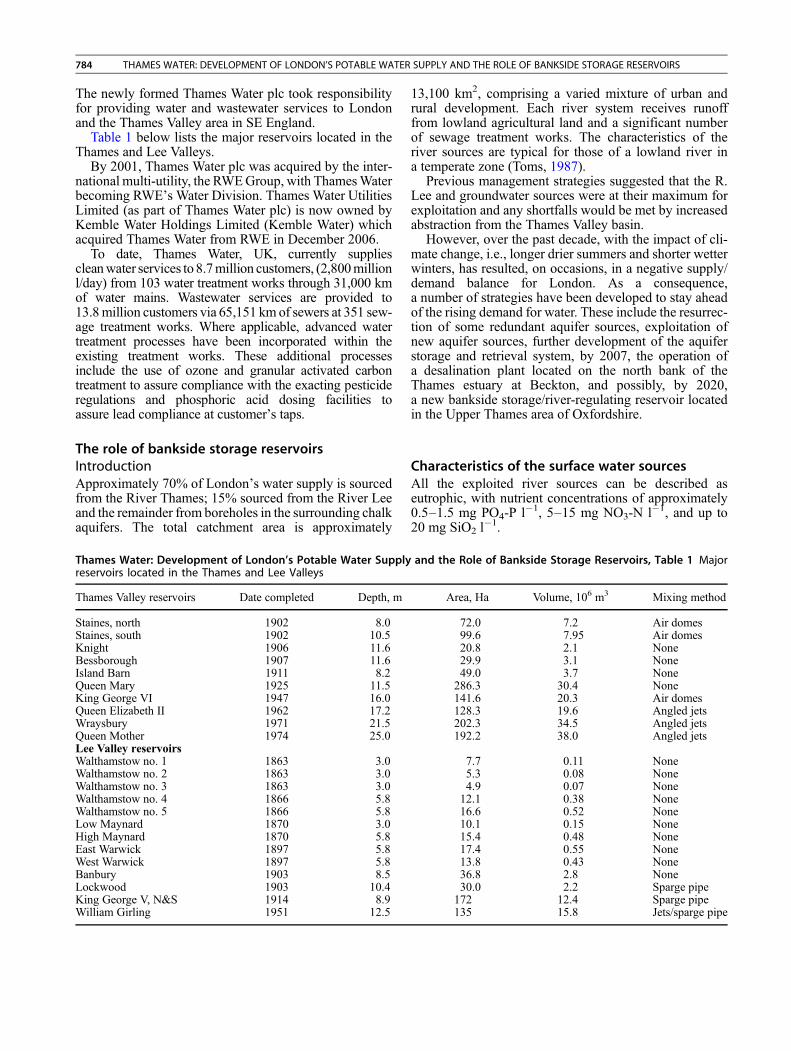
Tanganyika Lake, Modeling the Eco-hydrodynamics, Figure 4 Lastress varying by the factor indicated in the ordinate and ts, at h = 30wind stress and ts, at h = 70 m (d1–d4).

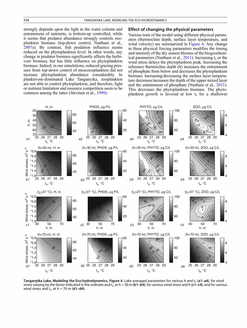
Effect of changing the physical parametersVarious tests of the model using different physical param-eters (thermocline depth, surface layer temperature, andwind velocity) are summarized in Figure 4. Any changein these physical forcing parameters modifies the timingand intensity of the dry season blooms of the biogeochem-ical parameters (Naithani et al., 2011). Increasing ts or thewind stress delays the phytoplankton peak. Increasing thereference thermocline depth (h) increases the entrainmentof phosphate from below and decreases the phytoplanktonbiomass. Increasing/decreasing the surface layer tempera-ture decreases/increases the depth of the upper mixed layerand the entrainment of phosphate (Naithani et al., 2011).This decreases the phytoplankton biomass. The phyto-plankton growth is favored at low ts for a shallower

ts, °C ts, °C

ts, °C ts, °C

ts, °C ts, °C

PHYTO, µg C/L

97

95 90

90

80

75

80

75a3 25 26 27 28 29

60

80

100ZOO, µg C/L

9

8.5

7.5

6.5

7

5.5

8.5

a4 25 26 27 28 294

6

8

(h=30 m), PHYTO, µg C/L

97

85

8065

90 90

b3 25 26 27 28 29

60

80

100(h=30 m), ZOO, µg C/L

7.5

7

5.5

7

6

b4 25 26 27 28 294

6

8

(ts=27 °C), PHYTO, µg C/L

91.2

97

80

80

7580

70

c3 30 50 70

60

80

100

h, mh, m

(ts=27 °C), ZOO, µg C/L

9

8

77

7.56.5

c4 30 50 704

6

8

(h=70 m), PHYTO, µg C/L

6080

85

80

75

d3 25 26 27 28 29

60

80

100(h=70 m), ZOO, µg C/L

56

6.5

8

d4 25 26 27 28 294

6

8

ke averaged parameters for various h and ts (a1–a4), for windm (b1–b4), for various wind stress and h (c1–c4), and for various

TANGANYIKA LAKE, MODELING THE ECO-HYDRODYNAMICS 775

thermocline and high ts at a deeper thermocline. Increas-ing wind stress favors phytoplankton production becauseof deeper mixing.

An increase in temperature will decrease the phyto-plankton and zooplankton biomass. This is because hightemperature will result in shallower thermoclines, therebydecreasing the mixing probabilities with the nutrient-richbottom water (Livingstone, 2003; Verburg et al., 2003;Verburg and Hecky, 2009). Lower temperature will leadto deeper lying thermocline thereby forcing the algal com-munity to spend more time in the low light conditions atgreater depths. Decreasing wind stress also hasa negative effect on the growth. However, if these hightemperatures are accompanied by stronger winds, theresulting wind mixing will bring the nutrients up to theeuphotic zone allowing a greater primary production.

ConclusionsThe behavior of the model-simulated parameters reflectsthat the dominant components responsible for the phyto-plankton biomass in the lake are temperature stratification,availability of light and nutrients. Primary production inthe nutrient-depleted surface layer depends upon therecycling of nutrients by wind-induced vertical mixing.The transport and mixing events are critical for theresupply of nutrients for the primary productivity and bio-geochemical processes in the stratified lake. Increasingstratification decreases mixing and entrainment of nutri-ents from the hypolimnion. At too high light conditionsat shallower depths, linked to higher surface layer temper-ature, the phytoplankton growth was limited by nutrients.Inversely, at higher nutrient levels at deeper depth, associ-ated with low surface layer temperature, phytoplanktonproduction was limited by light. The most favoring sur-face layer depth for the biomass production was found tobe between 40 and 60 m (Figure 4). This depth seems tobe linked to optimal light and nutrient conditions allowingphytoplankton production and an increase in its biomass.High winds are important for the supply of nutrients tothe euphotic zone in the Lake. They are also linked withincreased internal wave activities and turbulence. Thiscould induce an increased temporal patchiness in the pri-mary production (short moments when primary produc-tion could be very high). So the average seasonalcondition should not be considered when investigatingphytoplankton growth. But short-term strong wind eventscould also be important for local blooms in phytoplankton.

It can be inferred that a slight increase in temperaturewill still be bearable for Lake Tanganyika ecosystem, aslong as the wind is strong enough to mix water and bringnutrients from the hypolimnion to the epilimnion. Other-wise, the primary production will decrease.

BibliographyCoulter, G. W., and Spigel, R. H., 1991. Hydrodynamics. In

Coulter, G. W. (ed.), Lake Tanganyika and Its Life. London:Oxford University Press, pp. 49–75.

Hecky, R. E., and Fee, E. J., 1981. Primary production and rates ofalgal growth in Lake Tanganyika. Limnology and Oceanogra-phy, 26, 532–547.

Hecky, R. E., Spigel, R. H., and Coulter, G.W., 1991. Hydrodynam-ics. In Coulter, G. W. (ed.), Lake Tanganyika and Its Life.London: Oxford University Press, pp. 76–89.

Järvinen, M., Salonen, K., Sarvala, J., Vuorio, K., and Virtanen, A.,1999. The stoichiometry of particulate nutrients in LakeTanganyika– implications for nutrient limitation of phytoplankton.Hydrobiologia, 407, 81–88.

Johnson, T. C., and Odada, E. R., 1996. The Limnology, Climatologyand Paleoclimatology of the East African Lakes. Amsterdam:Gordon and Breach, p. 664.

Langenberg, V., Nyamushahu, S., Rooijackers, R., and Koelmans,A. A., 2003a. External nutrient sources for Lake Tanganyika.Journal of Great Lakes Research, 29, 169–180.

Langenberg, V., Sarvala, J., and Roijackers, R., 2003b. Effect ofwind induced water movements on nutrients, chlorophyll-a,and primary production in Lake Tanganyika. Aquatic EcosystemHealth & Management, 6(3), 279–288.

Livingstone, D. A., 2003. Global climate change strikes a TropicalLake. Science, 25, 468–469.

Naithani, J., and Deleersnijder, E., 2004. Are there internal Kelvinwaves in Lake Tanganyika? Geophysical Research Letters, 31,doi:10.1029/2003GL019156

Naithani, J., Deleersnijder, E., and Plisnier, P.-D., 2002. Origin ofintraseasonal variability in Lake Tanganyika. GeophysicalResearch Letters, 29, doi:10.1029/2002GL015843

Naithani, J., Deleersnijder, E., and Plisnier, P.-D., 2003. Analysis ofwind-induced thermocline oscillations of Lake Tanganyika.Environmental Fluid Mechanics, 3, 23–39.

Naithani, J., Darchambeau, F., Deleersnijder, E., Descy, J.-P., andWolanski, E., 2007a. Study of the nutrient and plankton dynam-ics in Lake Tanganyika using a reduced-gravity model. Ecolog-ical Modelling, 200, 225–233.

Naithani, J., Plisnier, P.-D., and Deleersnijder, E., 2007b. A simplemodel of the eco-hydrodynamics of the epilimnion of LakeTanganyika. Freshwater Biology, 52, 2087–2100.

Naithani, J., Plisnier, P.-D., and Deleersnijder, E., 2011. Possibleeffects of global climate change on the ecosystem of LakeTanganyika. Hydrobiologia, 671, 147–163.

Plisnier, P. D., and Descy, J.-P., 2005. Climlake: Climate variabilityas recorded in Lake Tanganyika. Final Report (2001–2005).FSPO – Global change, ecosystems and biodiversity: 105p.

Plisnier, P. D., Langenberg, V., Mwape, L., Chitamwebwa, D.,Tshibangu, K., and Coenen, E. J., 1996. Limnological samplingduring an annual cycle at three stations on Lake Tanganyika(1993–1994). FAO/FINNIDA Research for the Management ofthe Fisheries on Lake Tanganyika. GCP/RAF/271/FIN-TD/46(En), 124p.

Plisnier, P.-D., Chitamwebwa, D., Mwape, L., Tshibangu, K.,Langenberg, V., and Coenen, E., 1999. Limnological annualcycle inferred from physical-chemical fluctuations at three sta-tions of Lake Tanganyika. Hydrobiologia, 407, 45–58.

Price, J. F., 1979. On the scaling of stress-driven entrainment exper-iments. Journal of Fluid Mechanics, 90, 509–529.

Sarvala, J., Salonen, K., Järvinen, M., Aro, E., Huttula, T.,Kotilainen, P., Kurki, H., Langenberg, V., Mannini, P.,Peltonen, A., Plisnier, P.-D., Vuorinen, I., Mölsä, H., andLindqvist,O.V., 1999a. Trophic structure of LakeTanganyika: car-bon flows in the pelagic food web. Hydrobiologia, 407, 155–179.

Sarvala, J., Salonen, K., Mannini, P., Huttula, T., Plisnier, P.-D.,Langenberg, V., Vuorinen, I., Kurki, H., Mölsä, H., andLindqvist, O. V., 1999b. Chapter 8. Lake Tanganyika ecosystemassessment. FAO/FINNIDA Research for the management of theFisheries of Lake Tanganyika. GCP/RAF/271/FIN-TD/94 (En),pp. 68–73 (available from www.fao.org/fi/ltr).

776 TANGANYIKA LAKE: STRONG IN HYDRODYNAMICS, DIVERSE IN ECOLOGY

Verburg, P., and Hecky, R. E., 2009. The physics of warming ofLake Tanganyika by climate change. Limnology and Oceanog-raphy, 54, 2418–2430.

Verburg, P., Hecky, R. E., and Kling, H., 2003. Ecological conse-quences of a century of warming in Lake Tanganyika. Science,301, 505–507.

Cross-referencesAfrica, Lakes ReviewBasin-Scale Internal WavesCarbon Cycle in LakesCirculation Processes in LakesClimate Change: Factors Causing Variation or Change in theClimateInternal SeichesNutrient Balance, Light, and Primary ProductionStratification and Mixing in Tropical African LakesTanganyika Lake: Strong in Hydrodynamics, Diverse in EcologyThermal Regime of Lakes

TANGANYIKA LAKE: STRONG INHYDRODYNAMICS, DIVERSE IN ECOLOGY

Timo Huttula1, Jouko Sarvala21Freshwater Centre, Finnish Environment Institute,Jyväskylä, Finland2Department of Biology, University of Turku, Turku,Finland

IntroductionLake Tanganyika (Figure 1) is one of the few ancient lakesin the world (estimated age 9–12 million years; Cohenet al., 1993). It is the second in size of the African GreatLakes and also second in depth among lakes in the world.It locates at an altitude of 773 m above m.sl. The drainagearea is 263 000 km2. The lake is 650 km long and 50 kmwide in average. It has three main basins. In the north,the Kigoma basin extends to the depth of 1,310 m. Themiddle basin is separated from the Kigoma basin bya broad sill with a depth of 655 m, and in the south, fromthe Kipili basin by another sill with a depth of 700 m.The basin near Kipili is the deepest of the three basins,its maximum depth being 1,470 m. The lake is meromicticwith stable hypolimnetic waters, and the salt content islow for this type of lake (Coulter, 1991).

The early studies from the beginning of the last centuryhave been summarized by Coulter (1991). Later, a Belgianexploration in 1946–1947 proved the existence of internalwaves in the thermocline as they measured the lake watertemperature. Another result of the same expedition wasthe first bathymetric chart of the lake by Figure 1. In thelate 1950s, Dubois collected the first depth-time series oftemperature and oxygen data. In the early 1960s, Coulter(1963) continued the studies in the south, and later on, in1973–1975, in the northern part of the lake.

Lake Tanganyika was studied intensively during 1990sas part of the Lake Tanganyika Research for the Manage-ment of Fisheries (LTR) by FAO and also as part of Lake

Tanganyika Biodiversity Project/LTBP by UNDP/GEF(www.fao.org/fi/ltr (LTR) and http://www.ltbp.org/(LTBP)). Water level fluctuations and meteorologicaldata were collected at Bujumbura (Burundi), Kigoma(Tanzania), and Mpulungu (Zambia). Limited meteoro-logical observations were conducted also in Uvira (DRCongo), Kalemie (DR Congo), and Kipili (Tanzania).Data on the thermal regime of the lake waters werecollected with two moored buoy stations and also witha CTD-profiler near field stations, as well as from theresearch vessel during the expeditions. Data on water cur-rents were collected with flow cylinders, which were usedintensively near the field stations and also on lake-wideexpeditions. During LTBP, also acoustic Doppler currentprofilers (ADCP) were used both on board and at mooredstations.

Later four Finnish universities have arranged severalfield courses in Kigoma, Tanzania.

The CLIMLAKE “Climate Variability as Recorded byLake Tanganyika,” funded by the Belgian Science Policy,included a 3-year survey of the lake over the period2002–2004. Also hydrodynamic and ecological modelswere developed for the lake. The aim of the project wasto understand the Lake Tanganyika variability and sensi-tivity to climate change. Another Belgian project,CLIMFISH was active in years 2004–2006.

Meteorological conditionsThere are two main seasons with different weather condi-tions within the yearly cycle in the Lake Tanganyikaregion. The wet season from October to April is character-ized by weak winds over the lake, high humidity, consid-erable precipitation, and frequent thunderstorms(Figure 2). The dry season from May until the end ofAugust is characterized by little precipitation and strong,regular southerly winds. The seasonal changes of weatherand winds result from large-scale atmospheric processes,especially of the position of the global tropical windconvergence zone.

The diurnal cycle of winds is also well developed inTanganyika region. The studies of Savijärvi (1995 and1997) and Podsetchine et al. (1999) revealed that themountain slopes contributed about 50% and the tradewinds 25% to the diurnal variation of winds. The rest25% of the wind variation was due to the lake effect.The SE trade wind enhances the lake breeze considerablyat daytime and adds on the downslope winds at nighttime.

Thermal regimeThe seasonal thermal regime of the lake has beendiscussed by Capart (1952), Coulter (1963, 1991), Huttula(1997), Plisnier et al. (1999), Langenberg et al. (2002),Verburg et al. (2003), and Verburg and Hecky (2009).

Heating of the lake takes place mainly in the beginningof the wet season in October–November (Coulter, 1991;Huttula, 1997). Thermal stratification prevails all overthe lake. The thermocline is situated at the depth of

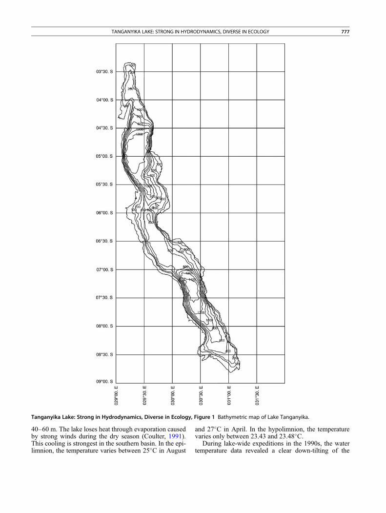
Tanganyika Lake: Strong in Hydrodynamics, Diverse in Ecology, Figure 1 Bathymetric map of Lake Tanganyika.

TANGANYIKA LAKE: STRONG IN HYDRODYNAMICS, DIVERSE IN ECOLOGY 777

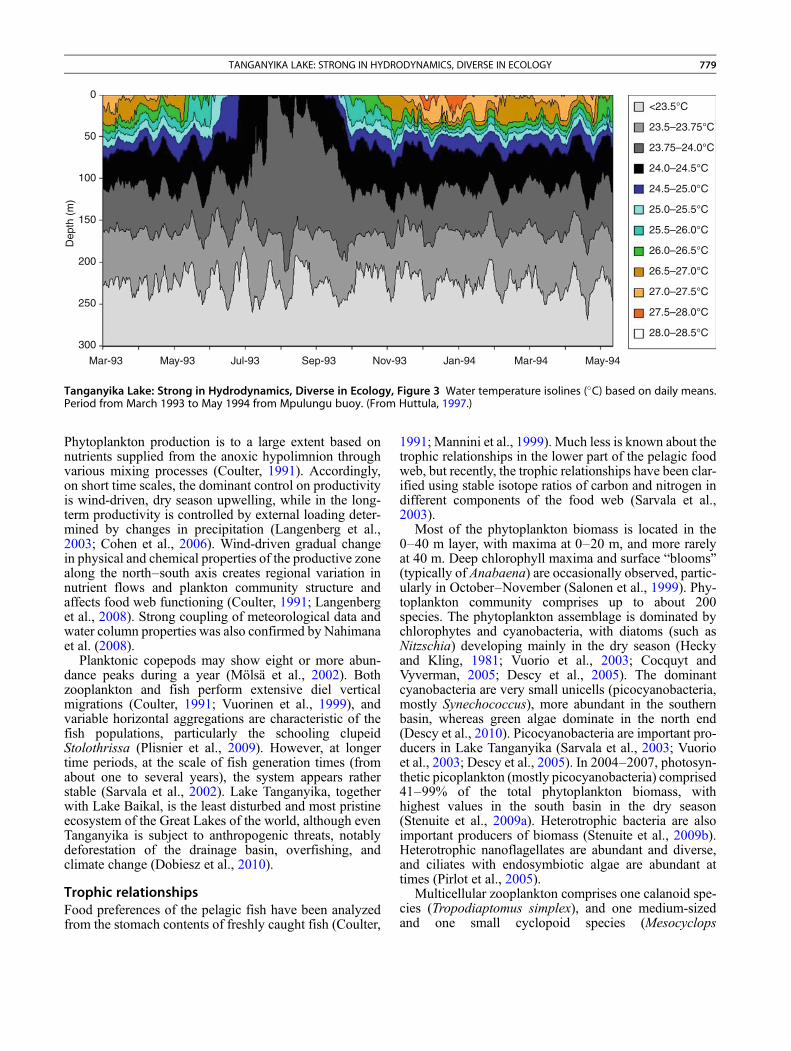
40–60 m. The lake loses heat through evaporation causedby strong winds during the dry season (Coulter, 1991).This cooling is strongest in the southern basin. In the epi-limnion, the temperature varies between 25�C in August

and 27�C in April. In the hypolimnion, the temperaturevaries only between 23.43 and 23.48�C.

During lake-wide expeditions in the 1990s, the watertemperature data revealed a clear down-tilting of the

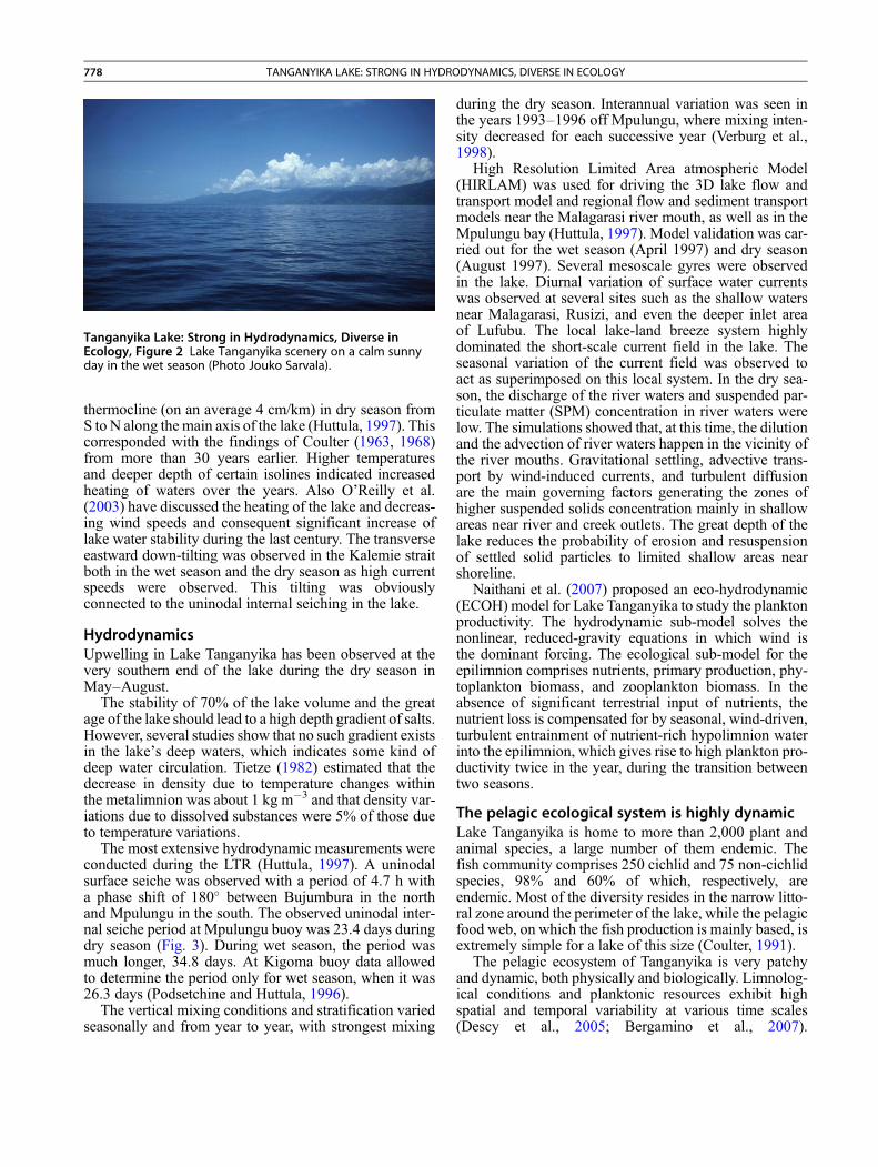
Tanganyika Lake: Strong in Hydrodynamics, Diverse inEcology, Figure 2 Lake Tanganyika scenery on a calm sunnyday in the wet season (Photo Jouko Sarvala).

778 TANGANYIKA LAKE: STRONG IN HYDRODYNAMICS, DIVERSE IN ECOLOGY

thermocline (on an average 4 cm/km) in dry season fromS to N along themain axis of the lake (Huttula, 1997). Thiscorresponded with the findings of Coulter (1963, 1968)from more than 30 years earlier. Higher temperaturesand deeper depth of certain isolines indicated increasedheating of waters over the years. Also O’Reilly et al.(2003) have discussed the heating of the lake and decreas-ing wind speeds and consequent significant increase oflake water stability during the last century. The transverseeastward down-tilting was observed in the Kalemie straitboth in the wet season and the dry season as high currentspeeds were observed. This tilting was obviouslyconnected to the uninodal internal seiching in the lake.

HydrodynamicsUpwelling in Lake Tanganyika has been observed at thevery southern end of the lake during the dry season inMay–August.

The stability of 70% of the lake volume and the greatage of the lake should lead to a high depth gradient of salts.However, several studies show that no such gradient existsin the lake’s deep waters, which indicates some kind ofdeep water circulation. Tietze (1982) estimated that thedecrease in density due to temperature changes withinthe metalimnion was about 1 kg m�3 and that density var-iations due to dissolved substances were 5% of those dueto temperature variations.

The most extensive hydrodynamic measurements wereconducted during the LTR (Huttula, 1997). A uninodalsurface seiche was observed with a period of 4.7 h witha phase shift of 180� between Bujumbura in the northand Mpulungu in the south. The observed uninodal inter-nal seiche period at Mpulungu buoy was 23.4 days duringdry season (Fig. 3). During wet season, the period wasmuch longer, 34.8 days. At Kigoma buoy data allowedto determine the period only for wet season, when it was26.3 days (Podsetchine and Huttula, 1996).

The vertical mixing conditions and stratification variedseasonally and from year to year, with strongest mixing

during the dry season. Interannual variation was seen inthe years 1993–1996 off Mpulungu, where mixing inten-sity decreased for each successive year (Verburg et al.,1998).

High Resolution Limited Area atmospheric Model(HIRLAM) was used for driving the 3D lake flow andtransport model and regional flow and sediment transportmodels near the Malagarasi river mouth, as well as in theMpulungu bay (Huttula, 1997). Model validation was car-ried out for the wet season (April 1997) and dry season(August 1997). Several mesoscale gyres were observedin the lake. Diurnal variation of surface water currentswas observed at several sites such as the shallow watersnear Malagarasi, Rusizi, and even the deeper inlet areaof Lufubu. The local lake-land breeze system highlydominated the short-scale current field in the lake. Theseasonal variation of the current field was observed toact as superimposed on this local system. In the dry sea-son, the discharge of the river waters and suspended par-ticulate matter (SPM) concentration in river waters werelow. The simulations showed that, at this time, the dilutionand the advection of river waters happen in the vicinity ofthe river mouths. Gravitational settling, advective trans-port by wind-induced currents, and turbulent diffusionare the main governing factors generating the zones ofhigher suspended solids concentration mainly in shallowareas near river and creek outlets. The great depth of thelake reduces the probability of erosion and resuspensionof settled solid particles to limited shallow areas nearshoreline.

Naithani et al. (2007) proposed an eco-hydrodynamic(ECOH) model for Lake Tanganyika to study the planktonproductivity. The hydrodynamic sub-model solves thenonlinear, reduced-gravity equations in which wind isthe dominant forcing. The ecological sub-model for theepilimnion comprises nutrients, primary production, phy-toplankton biomass, and zooplankton biomass. In theabsence of significant terrestrial input of nutrients, thenutrient loss is compensated for by seasonal, wind-driven,turbulent entrainment of nutrient-rich hypolimnion waterinto the epilimnion, which gives rise to high plankton pro-ductivity twice in the year, during the transition betweentwo seasons.

The pelagic ecological system is highly dynamicLake Tanganyika is home to more than 2,000 plant andanimal species, a large number of them endemic. Thefish community comprises 250 cichlid and 75 non-cichlidspecies, 98% and 60% of which, respectively, areendemic. Most of the diversity resides in the narrow litto-ral zone around the perimeter of the lake, while the pelagicfood web, on which the fish production is mainly based, isextremely simple for a lake of this size (Coulter, 1991).

The pelagic ecosystem of Tanganyika is very patchyand dynamic, both physically and biologically. Limnolog-ical conditions and planktonic resources exhibit highspatial and temporal variability at various time scales(Descy et al., 2005; Bergamino et al., 2007).

<23.5°C

23.5–23.75°C

23.75–24.0°C

24.0–24.5°C

24.5–25.0°C

25.0–25.5°C

25.5–26.0°C

26.0–26.5°C

26.5–27.0°C

27.0–27.5°C

27.5–28.0°C

28.0–28.5°C

May-94Mar-94Jan-94Nov-93Sep-93Jul-93May-93Mar-93

300

250

200

150

Dep

th (

m)

100

50

0

Tanganyika Lake: Strong in Hydrodynamics, Diverse in Ecology, Figure 3 Water temperature isolines (�C) based on daily means.Period from March 1993 to May 1994 from Mpulungu buoy. (From Huttula, 1997.)

TANGANYIKA LAKE: STRONG IN HYDRODYNAMICS, DIVERSE IN ECOLOGY 779

Phytoplankton production is to a large extent based onnutrients supplied from the anoxic hypolimnion throughvarious mixing processes (Coulter, 1991). Accordingly,on short time scales, the dominant control on productivityis wind-driven, dry season upwelling, while in the long-term productivity is controlled by external loading deter-mined by changes in precipitation (Langenberg et al.,2003; Cohen et al., 2006). Wind-driven gradual changein physical and chemical properties of the productive zonealong the north–south axis creates regional variation innutrient flows and plankton community structure andaffects food web functioning (Coulter, 1991; Langenberget al., 2008). Strong coupling of meteorological data andwater column properties was also confirmed by Nahimanaet al. (2008).

Planktonic copepods may show eight or more abun-dance peaks during a year (Mölsä et al., 2002). Bothzooplankton and fish perform extensive diel verticalmigrations (Coulter, 1991; Vuorinen et al., 1999), andvariable horizontal aggregations are characteristic of thefish populations, particularly the schooling clupeidStolothrissa (Plisnier et al., 2009). However, at longertime periods, at the scale of fish generation times (fromabout one to several years), the system appears ratherstable (Sarvala et al., 2002). Lake Tanganyika, togetherwith Lake Baikal, is the least disturbed and most pristineecosystem of the Great Lakes of the world, although evenTanganyika is subject to anthropogenic threats, notablydeforestation of the drainage basin, overfishing, andclimate change (Dobiesz et al., 2010).

Trophic relationshipsFood preferences of the pelagic fish have been analyzedfrom the stomach contents of freshly caught fish (Coulter,

1991; Mannini et al., 1999). Much less is known about thetrophic relationships in the lower part of the pelagic foodweb, but recently, the trophic relationships have been clar-ified using stable isotope ratios of carbon and nitrogen indifferent components of the food web (Sarvala et al.,2003).

Most of the phytoplankton biomass is located in the0–40 m layer, with maxima at 0–20 m, and more rarelyat 40 m. Deep chlorophyll maxima and surface “blooms”(typically of Anabaena) are occasionally observed, partic-ularly in October–November (Salonen et al., 1999). Phy-toplankton community comprises up to about 200species. The phytoplankton assemblage is dominated bychlorophytes and cyanobacteria, with diatoms (such asNitzschia) developing mainly in the dry season (Heckyand Kling, 1981; Vuorio et al., 2003; Cocquyt andVyverman, 2005; Descy et al., 2005). The dominantcyanobacteria are very small unicells (picocyanobacteria,mostly Synechococcus), more abundant in the southernbasin, whereas green algae dominate in the north end(Descy et al., 2010). Picocyanobacteria are important pro-ducers in Lake Tanganyika (Sarvala et al., 2003; Vuorioet al., 2003; Descy et al., 2005). In 2004–2007, photosyn-thetic picoplankton (mostly picocyanobacteria) comprised41–99% of the total phytoplankton biomass, withhighest values in the south basin in the dry season(Stenuite et al., 2009a). Heterotrophic bacteria are alsoimportant producers of biomass (Stenuite et al., 2009b).Heterotrophic nanoflagellates are abundant and diverse,and ciliates with endosymbiotic algae are abundant attimes (Pirlot et al., 2005).

Multicellular zooplankton comprises one calanoid spe-cies (Tropodiaptomus simplex), and one medium-sizedand one small cyclopoid species (Mesocyclops

780 TANGANYIKA LAKE: STRONG IN HYDRODYNAMICS, DIVERSE IN ECOLOGY

aequatorialis, Tropocyclops tenellus). Peculiarities ofTanganyika are several species of freshwater shrimps(from the genera Limnocaridina and Macrobrachium),and a medusa, Limnocnida tanganyicae (Coulter, 1991;Kurki et al., 1999).

Advanced developmental stages of Mesocyclops arepredatory. Tropodiaptomus is a herbivore, but it may feedon ciliates, too. Judging from their isotope signatures, thesmall cyclopoids and shrimps seem to be feeding onalgae, particularly cyanobacteria (Sarvala et al., 2003).Big shrimps prey upon zooplankton. The medusae feedon crustacean zooplankton, but they may contain highdensities of picocyanobacteria rendering the whole animalvisibly pink in color. In adequate light, such medusae arenet producers rather than consumers. The medusaehave no significant predators, thus being a dead end inthe food web.

Fish biology and fisheriesLake Tanganyika is renowned for its productive pelagicfishery, which is an important source of protein formillions of people in the surrounding area. About 45,000fishermen are directly engaged in fishing. In the 1990s,the total catches approached 200,000 t a�1 or about60 kg ha�1 a�1. Dried fish is sold >1,000 km away.The biological basis of the fishery was investigated in1992–2001 in a comprehensive ecosystem study“Research for the Management of the Fisheries on LakeTanganyika” (LTR; Mölsä et al., 1999; Mölsä et al.,2002; Sarvala et al., 1999).

There are three main types of fisheries in LakeTanganyika: industrial purse seines, artisanal lift nets,and various traditional methods, such as scoop nets,gillnets and hook and line (Coulter, 1991). Traditionalfishery yields a minor part of the total catch. Most fishingis done at night using light attraction. Major part of thecatch derives from the artisanal fishery in which two clu-peid species, Stolothrissa tanganicae and Limnothrissamiodon, compose about 65% of the total. The most impor-tant species in the lift-net fishery is Stolothrissa (max.length 12 cm), which spends most of its life in the pelagicarea, feeding mainly on copepod zooplankton and also onshrimps. Limnothrissa can grow to 17 cm, and feeds oncopepods, shrimps, and especially on young Stolothrissa.

A typical industrial fishing unit consists of a purseseiner, an auxiliary vessel for the seine, and 3–4 lampboats. At present, the industrial purse seine fishery targetsmainly Lates stappersii, the smallest of the four endemicLates (“perch”) species in Tanganyika. It can grow to50 cm long, but a typical size in the catch is 30–35 cm.Juvenile L. stappersii feed on zooplankton, but withincreasing size, they gradually switch to feeding onshrimps and fish, especially Stolothrissa. The otherlarge Lates species, L. mariae, L. microlepis, andL. angustifrons, all potentially growing to 50–100 cmlong, became sparse soon after the beginning of purseseining in the 1960s. L. mariae and L. angustifrons feedlargely on benthic fish and partly on shrimps and on the

small clupeids. L. microlepis is a specialized predator onStolothrissa.

There is an inverse correlation between the abundanceof Stolothrissa and L. stappersiiwhich is often interpretedas the consequence of predator–prey relations but maymainly reflect the underlying fluctuating limnologicalenvironment. Currently, the two species appear spatiallysegregated in the lake, S. tanganicae dominating in thenorth while L. stappersii is generally abundant in the southwhere it feeds mostly on shrimps. The abundance ofS. tanganicae is positively correlated to plankton biomass,while water transparency, depth of mixed layer, andoxygenated water appear important drivers for the abun-dance of L. stappersii (Plisnier et al., 2009).

The fishing pressure in Lake Tanganyika has steadilyincreased over the last decades. In the 1990s, the totallake-wide catches of Stolothrissa were estimated to beabout 25%, and those of Limnothrissa 30% of the calcu-lated production, suggesting that the present fishery ofthe planktivorous clupeids is sustainable. The harvest ratesof the Lates piscivores, in contrast, were extremely high,and excessive exploitation was likely to occur at leastlocally in the most intensively fished northern and south-ern ends of the lake (Sarvala et al., 2002; Mulimbwa,2006). According to bioenergetic calculations, the foodrequirements of the planktivorous fish were a reasonablefraction, 25–38%, of the zooplankton production. In con-trast, very high predation pressure was indicated on theshrimps and prey fish (Sarvala et al., 2002).

Estimates for primary production vary from 123to 662 g C m�2 a�1 (Sarvala et al., 1999; Stenuite et al.,2007). Bacterioplankton production is about 20–25% ofphytoplankton production (Sarvala et al., 1999; Stenuiteet al., 2009b). Zooplankton biomass (1 g C m�2) and pro-duction (23 g C m�2 a�1) suggest that the carbon transferefficiency from phytoplankton to zooplankton is low, incontrast to earlier speculations but in accordance withthe apparent importance of the microbial food web.Planktivorous fish biomass (0.4 g C m�2) and production(1.1 g C m�2 a�1) likewise indicate a low carbon transferefficiency from zooplankton into planktivorous fishproduction (Sarvala et al., 1999; Sarvala et al., 2002).Relatively low transfer efficiencies are not unexpected ina deep tropical lake because of the generally high meta-bolic losses due to the high temperatures and presumablyhigh costs of predator avoidance. The total fisheries yieldin Lake Tanganyika in the mid-1990s was 0.08–0.14%of pelagic primary production, i.e., within the range oftypical values in lakes (Sarvala et al., 1999).

Climate changeRecently, concerns have arisen on the possible effectsof climate warming on the productivity and fisheries ofTanganyika (O’Reilly et al., 2003; Verburg et al., 2003).Higher temperatures and lower wind stress could resultin increased stability of the water column and sharpeningof the vertical temperature gradient. The increased

TANGANYIKA LAKE: STRONG IN HYDRODYNAMICS, DIVERSE IN ECOLOGY 781

stability would then diminish mixing of hypolimneticnutrients into the euphotic zone and decrease primary pro-ductivity. There is a consensus about recent warming ofLake Tanganyika and several other East African lakesand its consequences to stratification, although the evi-dence is not unequivocal (Sarvala et al., 2006a; Sarvalaet al., 2006b; Verburg et al., 2006). The changing climateis ultimately expected to affect the fisheries yields, but sofar the observed variations in fish catches mainly reflectchanges in fishing practices and short-term environmentalfluctuations, not directional climate change (Sarvala et al.,2006a; Verburg et al., 2006), and even the postulateddecrease in primary production is as yet uncertain (Sarvalaet al., 2006b).

BibliographyBergamino, N., Loiselle, S. A., Cózarc, A., Dattilo, A. M.,

Bracchini, L., and Rossi, C., 2007. Examining the dynamics ofphytoplankton biomass in Lake Tanganyika using empiricalorthogonal functions. Ecological Modelling, 204, 156–162.

Capart, A., 1952. Le milieu géographique et géophysique, Résultatsscientifiques de l’exploration hydrobiologique du Lac Tanganika(1946–1947). Institut Royal des Sciences Naturelles deBelgique, 1, 3–27.

Cocquyt, C., and Vyverman, W., 2005. Phytoplankton in LakeTanganyika: a comparison of community composition and bio-mass off Kigoma with previous studies 27 years ago. Journalof Great Lakes Research, 31, 535–546.

Cohen, A. S., Soreghan, M. J., and Scholz, C. A., 1993. Estimatingthe age of formation of lakes: an example fromLake Tanganyika,East African rift system. Geology, 21, 511–514.

Cohen, A. S., Lezzar, K. E., Cole, J., Dettman, D., Ellis, G. S.,Eagle Gonneea, M., Plisnier, P.-D., Langenberg, V., Blaauw,M., and Zilifi, D., 2006. Late Holocene linkages betweendecade–century scale climate variability and productivity atLake Tanganyika, Africa. Journal of Paleolimnology, 36,189–209.

Coulter, G. W., 1963. Hydrological changes in relation to biologicalproduction in southern Lake Tanganyika. Limnology and Ocean-ography, 8, 463–477.

Coulter, G. W., 1968. Hydrological processes and primary produc-tion in Lake Tanganyika. In Proceedings of the 11th Conferenceon Great Lakes Research. International Association for GreatLakes Research, pp. 609–626.

Coulter, G. W. (ed.), 1991. Lake Tanganyika and Its Life. London/New York: British Museum, Natural History/Oxford UniversityPress.

Descy, J.-P., Hardy, M. A., Stenuite, S., Pirlot, S., Leporcq, B.,Kimirey, I., Sekadende, B., Mwaitega, S. R., and Sinyenza, D.,2005. Phytoplankton pigments and community composition inLake Tanganyika. Freshwater Biology, 50, 668–684.

Descy, J.-P., Tarbe, A.-L., Stenuite, S., Pirlot, S., Stimart, J.,Vanderheyden, J., Leporcq, B., Stoyneva, M. P., Kimirei, I.,Sinyinza, D., and Plisnier, P.-D., 2010. Drivers of phytoplanktondiversity in Lake Tanganyika. Hydrobiologia, 653, 29–44.

Dobiesz, N. E., Hecky, R. E., Johnson, T. B., Sarvala, J.,Dettmers, J. M., Lehtiniemi, M., Rudstam, L. G.,Madenjian, C. P., and Witte, F., 2010. Metrics of ecosystemstatus for large aquatic systems – a global comparison. Journalof Great Lakes Research, 36, 123–138.

Hecky, R. E., and Kling, H. J., 1981. The phytoplankton andprotozooplankton of the euphotic zone of Lake Tanganyika:species composition, biomass, chlorophyll content, and

spatio-temporal distribution. Limnology and Oceanography,26, 548–564.

Huttula, T. (ed.), 1997. Flow, Thermal Regime and Sediment Trans-port Studies in Lake Tanganyika. Kuopio: Kuopio UniversityPublications C, Natural and Environmental Sciences, Vol. 73,ISBN 951-781-711-8, ISSN 1235–0486.

Kurki, H., Vuorinen, I., Bosma, E., and Bwebwa, D., 1999. Spatialand temporal changes in copepod zooplankton communities ofLake Tanganyika. Hydrobiologia, 407, 105–114.

Langenberg, V. T., Mwape, L., Thsibangu, K., Tumba, J. M.,Koelmans, A. A., Roijackers, R., Salonen, K., Sarvala, J., andMölsä, H., 2002. Comparison of thermal stratification, lightattenuation, and chlorophyll-a dynamics between the ends ofLake Tanganyika. Aquatic Ecosystem Health & Management,5, 255–265.

Langenberg, V. T., Nyamushahu, S., Roijackers, R., andKoelmans, A. A., 2003. External nutrient sources for LakeTanganyika. Journal of Great Lakes Research, 29, 169–180.

Langenberg, V. T., Tumba, J.-M., Tshibangu, K., Lukwesa, C.,Chitamwebwa, D., Bwebwa, D., Makasa, L., and Roijackers, R.,2008. Heterogeneity in physical, chemical and plankton-community structures in Lake Tanganyika. Aquatic EcosystemHealth & Management, 11, 16–28.

Mannini, P., Katonda, I., Kissaka, B., and Verburg, P., 1999. Feed-ing ecology of Lates stappersii in Lake Tanganyika.Hydrobiologia, 407, 131–139.

Mölsä, H., Reynolds, E., Coenen, E., and Lindqvist, O. V., 1999.Fisheries research towards resource management on LakeTanganyika. Hydrobiologia, 407, 1–24.

Mölsä, H., Sarvala, J., Badende, S., Chitamwebwa, D., Kanyaru, R.,Mulimbwa, N., and Mwape, L., 2002. Ecosystem monitoring inthe development of sustainable fisheries in Lake Tanganyika.Aquatic Ecosystem Health & Management, 5, 267–281.

Mulimbwa, N., 2006. Assessment of the commercial artisanal fish-ing impact on three endemic pelagic fish stocks of Stolothrissatanganicae, Limnothrissa miodon and Lates stappersii inBujumbura and Kigoma subbasins of Lake Tanganyika.Verhandlungen Internationale Vereinigung für Limnologie, 29,1189–1193.

Nahimana, D., Brion, N., Baeyens, W., and Ntakimazi, G., 2008.General nutrient distribution in the water column of NorthernLake Tanganyika. Aquatic Ecosystem Health & Management,11, 8–15.

Naithani, J., Plisnier, P.-D., and Deleersnijder, E., 2007. A simplemodel of the eco-hydrodynamics of the epilimnion of LakeTanganyika. Freshwater Biology, 52, 2087–2100.

O’Reilly, C. M., Alin, S. R., Plisnier, P.-D., Cohen, A. S., andMcKee, B. A., 2003. Climate change decreases aquatic ecosys-tem productivity of Lake Tanganyika, Africa. Nature, 424,766–768.

Pirlot, S., Vanderheyden, J., Descy, J.-P., and Servais, P., 2005.Abundance and biomass of heterotrophic micro-organisms inLake Tanganyika. Freshwater Biology, 50, 1219–1232.

Plisnier, P.-D., Chitamwebwa, D., Mwape, L., Tshibangu, K.,Langenberg, V., and Coenen, E., 1999. Limnological annualcycle inferred from physical-chemical fluctuations at threestations of Lake Tanganyika. Hydrobiologia, 407, 45–58.

Plisnier, P.-D., Mgana, H., Kimirei, I., Chande, A., Makasa, L.,Chimanga, J., Zulu, F., Cocquyt, C., Horion, S., Bergamino, N.,Naithani, J., Deleersnijder, E., André, L., Descy, J.-P., andCornet, Y., 2009. Limnological variability and pelagic fishabundance (Stolothrissa tanganicae and Lates stappersii) inLake Tanganyika. Hydrobiologia, 625, 117–134.

Podsetchine, V., and Huttula, T., 1996. Hydrological Modelling:Activity Report for the Period of 1.4.–30.9.95. Bujumbura:FAO/FINNIDA Research for the Management of the Fisherieson Lake Tanganyika, GCP/RAF/271/FIN-TD/45 (En).

782 THAMES WATER: DEVELOPMENT OF LONDON’S POTABLE WATER SUPPLY AND THE ROLE OF BANKSIDE STORAGE RESERVOIRS

Podsetchine, V., Huttula, T., and Savijärvi, H., 1999. A three-dimensional circulation model of Lake Tanganyika.Hydrobiologia, 407, 25–35.

Salonen, K., Sarvala, J., Järvinen,M., Langenberg, V., Nuottajärvi, M.,Vuorio, K., and Chitamwebwa, D. B. R., 1999. Phytoplankton inLake Tanganyika – vertical and horizontal distribution of in vivofluorescence. Hydrobiologia, 407, 89–103.

Sarvala, J., Salonen, K., Järvinen, M., Aro, E., Huttula, T.,Kotilainen, P., Kurki, H., Langenberg, V., Mannini, P.,Peltonen, A., Plisnier, P.-D., Vuorinen, I., Mölsä, H., andLindqvist, O. V., 1999. Trophic structure of Lake Tanganyika:carbon flows in the pelagic food web. Hydrobiologia, 407,155–179.

Sarvala, J., Tarvainen, M., Salonen, K., and Mölsä, H., 2002.Pelagic food web as the basis of fisheries in Lake Tanganyika:a bioenergetic modeling analysis. Aquatic Ecosystem Health &Management, 5, 283–292.

Sarvala, J., Badende, S., Chitamwebwa, D., Juvonen, P., Mwape, L.,Mölsä, H., Mulimbwa, N., Salonen, K., Tarvainen, M.,and Vuorio, K., 2003. Size-fractionated d15N and d13C isotoperatios elucidate the role of the microbial food web in the pelagialof Lake Tanganyika. Aquatic Ecosystem Health &Management,6, 241–250.

Sarvala, J., Langenberg, V. T., Salonen, K., Chitamwebwa, D.,Coulter, G. W., Huttula, T., Kanyaru, R., Kotilainen, P.,Makasa, L., Mulimbwa, N., and Mölsä, H., 2006a. Fish catchesfrom Lake Tanganyika mainly reflect changes in fishery prac-tices, not climate. Verhandlungen Internationale Vereinigungfür Limnologie, 29, 1182–1188.

Sarvala, J., Langenberg, V. T., Salonen, K., Chitamwebwa, D.,Coulter, G. W., Huttula, T., Kotilainen, P., Mulimbwa, N., andMölsä, H., 2006b. Changes in dissolved silica and transparencyare not sufficient evidence for decreased primary productivitydue to climate warming in Lake Tanganyika. Reply to commentby Verburg, Hecky and Kling. Verhandlungen InternationaleVereiningung für Limnologie, 29, 2339–2342.

Savijärvi, H., 1995. Sea-breeze effects on large-scale atmosphericflow. Contributions to Atmospheric Physics, 68, 281–292.

Savijärvi, H., 1997. Diurnal winds around Lake Tanganyika.Quarterly Journal of the Royal Meteorological Society, 123,901–918.

Stenuite, S., Pirlot, S., Hardy, M.-A., Sarmento, H., Tarbe, A.-L.,Leporcq, B., and Descy, J.-P., 2007. Phytoplankton productionand growth rate in Lake Tanganyika: evidence of a decline in pri-mary productivity in recent decades. Freshwater Biology, 52,2226–2239.

Stenuite, S., Tarbe, A.-L., Sarmento, H., Unrein, F., Pirlot, S.,Sinyinza, D., Thill, S., Lecomte, M., Leporcq, B., Gasol, J. M.,and Descy, J.-P., 2009a. Photosynthetic picoplankton in LakeTanganyika: biomass distribution patterns with depth, seasonand basin. Journal of Plankton Research, 31, 1531–1544.

Stenuite, S., Pirlot, S., Tarbe, A.-L., et al., 2009b. Abundance andproduction of bacteria, and relationship to phytoplankton pro-duction, in a large tropical lake (Lake Tanganyika). FreshwaterBiology, 54, 1300–1311.

Tietze, K. L., 1982. Results of the Lake Tanganyika investigations inDecember, 1981, Memo No: 93356. Hannover: Bundesanstaltfur Geowissenschaften und Rohstoffe.

Verburg, P., and Hecky, R. E., 2009. The physics of the warming ofLake Tanganyika by climate change. Limnology and Oceanog-raphy, 54, 2418–2430.

Verburg, P., Kakogozo, B.,Makasa, L., Muhoza, S., and Tomba J. -M.,1998.Hydrodynamics of Lake Tanganyika 1993–1996. Synopsisand Interannual Comparisons. Bujumbura: FAO/FINNIDAResearch for the Management of the Fisheries on LakeTanganyika, GCP/RAF/271/FIN-TD/87 (En).

Verburg, P., Hecky, R. E., and Kling, H., 2003. Ecological conse-quences of a century of warming in Lake Tanganyika. Science,301, 505–507.

Verburg, P., Hecky, R. E., and Kling, H., 2006. Climate warmingdecreased primary productivity in Lake Tanganyika, inferredfrom accumulation of dissolved silica and increased transpar-ency. Verhandlungen Internationale Vereinigung fürLimnologie, 29, 2335–2338.

Vuorinen, I., Kurki, H., Bosma, E., Kalangali, A., Mölsä, H., andLindqvist, O. V., 1999. Vertical distribution and migration ofpelagic Copepoda in Lake Tanganyika. Hydrobiologia, 407,115–121.

Vuorio, K., Nuottajärvi, M., Salonen, K., and Sarvala, J., 2003.Spatial distribution of phytoplankton and picocyanobacteria inLake Tanganyika in March and April 1998. Aquatic EcosystemHealth & Management, 6, 263–278.

Cross-referencesAfrica, Lakes ReviewClimate Change: Factors Causing Variation or Change in theClimateInternal SeichesSedimentation Processes in LakesStratification and Mixing in Tropical African LakesTanganyika Lake, Modeling the Eco-hydrodynamicsThermal Regime of LakesThermobaric Stratification of Very Deep Lakes

THAMES WATER: DEVELOPMENT OF LONDON’SPOTABLE WATER SUPPLY AND THE ROLE OFBANKSIDE STORAGE RESERVOIRS

Phil Renton1, Terry Bridgman1, Robin G. Bayley21Asset Management, Thames Water, Walton AdvancedTreatment Works, Walton on Thames, Surrey, UK2Thames Water, Kempton Park WTW’s, Feltham,Middlesex, UK

Historical perspectivePredecessor organizations of Thames Water could be saidto date back to circa 1582, when the City Corporationgranted permission to Peter Morice, a Dutchman, to leasean arch of London Bridge, where water wheels wereconstructed, to pump R. Thames water to local housingthrough a series of wood, and later, lead pipes. This systemestablished the first water supply company in the country –the London Water Works (2005).

By the end of the sixteenth century, the population ofLondon had swelled to approximately 180,000 residents,and London now faced an acute shortage of clean drinkingwater.

By the turn of the century, Edward Colthurst, a formerarmy captain, devised plans to transfer water by gravityfrom springs in Hertfordshire to Islington in NorthLondon. This was to become the New River (2005).

In 1602, Colthurst received support for the project fromthe City Corporation, but Queen Elizabeth 1 wasconcerned that navigation in the R. Lee may suffer.

THAMES WATER: DEVELOPMENT OF LONDON’S POTABLE WATER SUPPLY AND THE ROLE OF BANKSIDE STORAGE RESERVOIRS 783

A commission was established to investigate these issues,but the Queen died before Colthurst was granted a licenseto start the work.

In 1604, James 1st granted permission for the work tostart provided the New River was no more than 6 ft wideand the work was finished within 7 years.

By 1605, only three miles had been completed, andColthurst required further funding from the City Corpora-tion. The funding debate dragged on for the next 3 years,when in 1609, the Corporation accepted an offer fromHugh Myddelton to complete the work in four years.

The 40 mile New River was designed to follow the100 ft contour from Chadwell Spring, in HertfordshireHerts to the Round Pond at New River Head in Islington.

On Sept 29th, 1613, in the presence of local dignitaries,the New River was opened by the Lord Mayor of London,and the New River Water Company was established.

Fresh water could now be supplied to local residents viaa series of fifty eight water mains made from elm treetrunks. One-inch bore lead pipes delivered water to thosecustomers who could afford to pay for the service.

During the eighteenth and nineteenth century, variousdevelopments in London’s water supply where affectedincluding the construction of an Upper Pond at the NewRiver Head, straightening the course of the New River,and the establishment of eight water companies supplyingthe Metropolitan area, namely:

Company

Date founded

The New River Company

1619 The Chelsea Waterworks Company 1723 The West Middlesex Waterworks Company 1806 The East London Waterworks Company 1807 The Grand Junction Waterworks Company 1811 The Lambeth Waterworks Company 1785 The Kent Waterworks Company 1809 The Southwark and Vauxhall Waterworks Company 1760

However, concerns about the purity of water wereraised after a further outbreak of cholera in 1849 whenDr. John Snow famously determined the causal linkbetween contaminated water and water-related disease,originating from the Broad St. well in Soho. Asa consequence, water companies were required to meetnew statutory demands, and in 1852, the MetropolisWaterAct was established.

The Act determined that all water companies mustabstract R. Thames water above Teddington weir (the tidallimit), that all river water must be filtered, and all filteredwater must be stored in covered reservoirs.

In 1871, revisions of the Metropolis Water Actdetermined that water supplies were to be constant, domesticplumbing standards were implemented, and the first “waterexaminer” was appointed.

In 1904, the Metropolitan Water Board (MWB) wasestablished which took over the responsibilities for water

supply from all the previous water companies. Ten yearslater, the MWB built its new headquarters on the site of theRound Pond in Islington. It was named New River Head.

Prior to the establishment of the MWB, a number of theprevious water companies had erected river waterpumping stations in the Lower Thames and Lee Valleys.They were located above the tidal limits of both riversand designed to pump to a series of small bankside storagereservoirs which had been constructed upstream of theassociated water treatment works.

The reservoirs were commonly named after the individualcompanies, and some are still in operation in the twenty-firstcentury.

For example, at Hampton WTWs, in the Lower ThamesValley, one of the earliest reservoirs built is still in use asa balancing tank at the head of the water treatment works.This “reservoir,” built in 1879, was named the Grand Junc-tion reservoir after the original water company. Close by arethe redundant Stain Hill reservoirs, constructed in 1898.

Further, to the west, at Kempton Park WTW’s, twoadditional reservoirs were constructed in 1906, namely,the Kempton Park East and West reservoirs.

South of the R. Thames at the Walton on Thames treat-ment works are four reservoirs which were constructed bythe Chelsea Water Company in 1877. Next to them are thefour Lambeth Water Company reservoirs, two of whichwere built in 1874 and the others in 1901 and 1903.

These small reservoirs are now redundant, and follow-ing a period of major gravel abstraction, the area will beconverted to a wildlife and wetlands nature reserve.

Between 1863 and 1903, in the LeeValley area, NELon-don, 11 small storage reservoirs were constructed (details inTable 2, below). They are all in operational use today, eitheras water supply reservoirs or as sedimentation basins forwash water originating from the Coppermills WTWs.

After 1904, the management of the reservoir complexbecame the responsibility of the Metropolitan WaterBoard. The MWB inherited a combined storage volumein the Thames Valley of 196 � 106 m3.

The 1973 Water Act simplified the way that water andwastewater services were provided in the UK and pavedthe way for the creation of ten major Water Authoritiesin 1974.

By the time the Thames Water Authority had replacedthe MWB, the ongoing reservoir storage strategy hadensured an additional storage capacity of 150 � 106 m3,equivalent to approx.100 days supply to Greater London.

Of the 25 reservoirs originally adopted in 1974, ten stra-tegic reservoirs in the Lower Thames Valley area are thoseprimarily considered in anymanagement decision process.

These ten reservoirs provide a total storage volume of165.1 � 106 m3, five of which are of prime importancefor water resources in that they contain, individually, morethan 19 � 106 m3 and comprise 82.5% of the total LowerThames Valley storage volume.

In 1989, a revision of the UK Water Act enabled partsof the UK water industry to be passed to the private sector.

784 THAMES WATER: DEVELOPMENT OF LONDON’S POTABLE WATER SUPPLY AND THE ROLE OF BANKSIDE STORAGE RESERVOIRS

The newly formed Thames Water plc took responsibilityfor providing water and wastewater services to Londonand the Thames Valley area in SE England.

Table 1 below lists the major reservoirs located in theThames and Lee Valleys.

By 2001, Thames Water plc was acquired by the inter-national multi-utility, the RWEGroup, with ThamesWaterbecoming RWE’s Water Division. Thames Water UtilitiesLimited (as part of Thames Water plc) is now owned byKemble Water Holdings Limited (Kemble Water) whichacquired Thames Water from RWE in December 2006.

To date, Thames Water, UK, currently suppliescleanwater services to 8.7million customers, (2,800millionl/day) from 103 water treatment works through 31,000 kmof water mains. Wastewater services are provided to13.8million customers via 65,151 km of sewers at 351 sew-age treatment works. Where applicable, advanced watertreatment processes have been incorporated within theexisting treatment works. These additional processesinclude the use of ozone and granular activated carbontreatment to assure compliance with the exacting pesticideregulations and phosphoric acid dosing facilities toassure lead compliance at customer’s taps.

The role of bankside storage reservoirsIntroductionApproximately 70% of London’s water supply is sourcedfrom the River Thames; 15% sourced from the River Leeand the remainder from boreholes in the surrounding chalkaquifers. The total catchment area is approximately

Thames Water: Development of London’s Potable Water Supplyreservoirs located in the Thames and Lee Valleys

Thames Valley reservoirs Date completed Depth, m

Staines, north 1902 8.0Staines, south 1902 10.5Knight 1906 11.6Bessborough 1907 11.6Island Barn 1911 8.2Queen Mary 1925 11.5King George VI 1947 16.0Queen Elizabeth II 1962 17.2Wraysbury 1971 21.5Queen Mother 1974 25.0Lee Valley reservoirsWalthamstow no. 1 1863 3.0Walthamstow no. 2 1863 3.0Walthamstow no. 3 1863 3.0Walthamstow no. 4 1866 5.8Walthamstow no. 5 1866 5.8Low Maynard 1870 3.0High Maynard 1870 5.8East Warwick 1897 5.8West Warwick 1897 5.8Banbury 1903 8.5Lockwood 1903 10.4King George V, N&S 1914 8.9William Girling 1951 12.5

13,100 km2, comprising a varied mixture of urban andrural development. Each river system receives runofffrom lowland agricultural land and a significant numberof sewage treatment works. The characteristics of theriver sources are typical for those of a lowland river ina temperate zone (Toms, 1987).

Previous management strategies suggested that the R.Lee and groundwater sources were at their maximum forexploitation and any shortfalls would be met by increasedabstraction from the Thames Valley basin.

However, over the past decade, with the impact of cli-mate change, i.e., longer drier summers and shorter wetterwinters, has resulted, on occasions, in a negative supply/demand balance for London. As a consequence,a number of strategies have been developed to stay aheadof the rising demand for water. These include the resurrec-tion of some redundant aquifer sources, exploitation ofnew aquifer sources, further development of the aquiferstorage and retrieval system, by 2007, the operation ofa desalination plant located on the north bank of theThames estuary at Beckton, and possibly, by 2020,a new bankside storage/river-regulating reservoir locatedin the Upper Thames area of Oxfordshire.

Characteristics of the surface water sourcesAll the exploited river sources can be described aseutrophic, with nutrient concentrations of approximately0.5–1.5 mg PO4-P l�1, 5–15 mg NO3-N l�1, and up to20 mg SiO2 l

�1.

and the Role of Bankside Storage Reservoirs, Table 1 Major

Area, Ha Volume, 106 m3 Mixing method

72.0 7.2 Air domes99.6 7.95 Air domes20.8 2.1 None29.9 3.1 None49.0 3.7 None286.3 30.4 None141.6 20.3 Air domes128.3 19.6 Angled jets202.3 34.5 Angled jets192.2 38.0 Angled jets

7.7 0.11 None5.3 0.08 None4.9 0.07 None12.1 0.38 None16.6 0.52 None10.1 0.15 None15.4 0.48 None17.4 0.55 None13.8 0.43 None36.8 2.8 None30.0 2.2 Sparge pipe172 12.4 Sparge pipe135 15.8 Jets/sparge pipe

THAMES WATER: DEVELOPMENT OF LONDON’S POTABLE WATER SUPPLY AND THE ROLE OF BANKSIDE STORAGE RESERVOIRS 785

During periods of mod-high flow, the river can alsocontain high organic carbon and silt loadings, rangingbetween 0.5 and 6.0 g C·m3, and turbidity values rangingfrom 10 to 100 NTU.

The river systems can also support a range of microbio-logical and algal species at varying concentrations depen-dant on the rainfall values, flow conditions, and seasonimpacts. In spring and summer when flows are lower,the river can be highly productive with phytoplanktonbiomasses values in excess of 200 mg-Chla/m3 recorded,the dominant algal species generally the centric diatom,Stephanodiscus hantzschii.

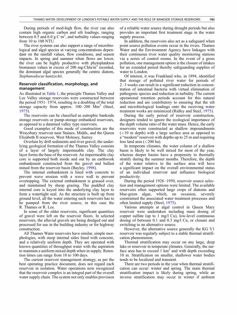
Reservoir classification, morphology, andmanagementAs illustrated in Table 1, the principle Thames Valley andLee Valley storage reservoirs were constructed betweenthe period 1951–1974, resulting in a doubling of the totalstorage capacity from approx. 100–200 Mm3 (Steel,1975).

The reservoirs can be classified as eutrophic banksidestorage reservoirs or pump-storage embanked reservoirs,as opposed to a dammed valley type reservoirs.

Good examples of this mode of construction are theWraysbury reservoir near Staines, Middx, and the QueenElizabeth II reservoir, West Molesey, Surrey.

Overlain by drift sediments and river gravel, the under-lying geological formation of the Thames Valley consistsof a layer of largely impermeable clay. The claylayer forms the base of the reservoir. An impermeable claycore is supported both inside and out by an earthworkembankment constructed from the gravel and ballastmined from the reservoir basin (Bayley, 1998).

The internal embankment is lined with concrete toprevent wave erosion with a wave wall to preventovertopping. The external embankment is grassed over,and maintained by sheep grazing. The puddled clayinternal core is keyed into the underlying clay layer toform a watertight seal. As the structure is built up fromground level, all the water entering such reservoirs has tobe pumped from the river source, in this case theR. Thames or R. Lee.

In some of the older reservoirs, significant quantitiesof gravel were left on the reservoir floors. In selectedreservoirs, the alluvial gravels are being dredged out andprocessed for use in the building industry or for highwayconstruction.

All Thames Water reservoirs have similar, simple mor-phologies, with steep internal sides lined with concrete,and a relatively uniform depth. They are operated withknown quantities of throughput water with the aspirationto maintain a uniform mixed depth when in supply. Reten-tion times can range from 10 to 100 days.

The current reservoir management strategy, as per thebest operating practice document, does not regard eachreservoir in isolation. Water operations now recognizedthat the reservoir complex is an integral part of the overallwater supply chain. The system not only enables provision

of a reliable water source during drought periods but alsoprovides an important first treatment stage in the watersupply process.

In addition, the reservoirs also act as a safeguard whenpoint source pollution events occur in the rivers. ThamesWater and the Environment Agency have linkages withtheir continuous river water quality monitoring stationsvia a series of control rooms. In the event of a grosspollution, one management option is the closure of intakesfor an extended period thereby safeguarding supplies ofwater to London.

Of interest, it was Frankland who, in 1894, identifiedthat storage of polluted river water for periods of2–3 weeks can result in a significant reduction in concen-tration of intestinal bacteria with virtual elimination ofpathogenic species and reduction in turbidity. The currentoperational retention periods account for this naturalreduction and are contributory to ensuring that the siltand microbiological loadings onto the receiving watertreatment works are minimized (Ridley and Steel, 1975).

During the early period of reservoir construction,designers tended to ignore the ecological importance ofthe depth volume ratio of the water mass. Hence, the earlyreservoirs were constructed as shallow impoundments(<10 m depth) with a large surface area as opposed toa “modern” reservoir with depths up to 25 m and requiringless land area (<200 ha).

In temperate climates, the water column of a shallowbasin is likely to be well mixed for most of the year,whereas deeper basins have a propensity to thermallystratify during the summer months. Therefore, the depthof the water relative to the surface area will havea significant impact on the overall environmental statusof an individual reservoir and influence biologicalproductivity.

During the period 1926–1950, reservoir source selec-tion and management options were limited. The availablereservoirs often supported large crops of diatoms andblue-green algae, which, on occasion, severelyconstrained the associated water treatment processes andoften limited supply (Steel, 1975).

Various attempts at algal control in Queen Maryreservoir were undertaken including mass dosing ofcopper sulfate (up to 1 mg/l Cu), low-level continuousdosing of between 0.1 and 0.3 mg/l Cu, or closure andswitching to an alternative source.

However, the alternative source generally the KG V1reservoir was regularly subject to a stable thermal stratifi-cation phenomenon.

Thermal stratification may occur on any large, deeplake or reservoir in temperate climates. Generally, the sur-face area has to exceed 1 km2 and with depth exceeding10 m. Stratification on smaller, shallower water bodiestends to be localized and transient.

There are two periods in the year when thermal stratifi-cation can occur: winter and spring. The main thermalstratification impact is likely during spring, while aninverse stratification may occur in winter if ambient

786 THAMES WATER: DEVELOPMENT OF LONDON’S POTABLE WATER SUPPLY AND THE ROLE OF BANKSIDE STORAGE RESERVOIRS

temperatures are low for an extended period, then thereservoirs can ice over.

Reservoirs that stratify once a year are termed“monomictic,” while those that regularly stratify twicea year are termed “dimictic.”

Thermal stratification of a water body results becausewater has a maximum density at 4 �C and that waterhas a high specific heat (approximately 4.2 J.g�1.��C).During spring and early summer, the upper layers of thewater column are warmed and, as a result, become lessdense. Gradually, a distinct layered structure develops inthe water column with a warm top layer, a cold denserdeep layer with a dividing region between these layerscalled the thermocline, characterized by a temperaturechange of 1.0 or more degrees Celsius per meter depth.

The warm upper layer is known as the epilimnion andthe cold dense layer, the hypolimnion. The thermoclineacts as an almost frictionless layer and also forms as aneffective barrier to rapid diffusion of chemical species.In deep basins, this thermal stratification is stable due tothe low center of gravity of the water column.

Algal growth under these conditions can only takeplace where there is sufficient light for photosynthesis.The algal populations may grow until limited by the avail-able light (self shading) or other ecological factors such asgrazing by zooplankton and the impact of high fishbiomasses.

As the available light energy reduces exponentiallywith depth, then the euphotic depth (m) is defined asthe depth at which useful light or “photosynthetic activeradiation” (PhAR) can penetrate.

The rate at which light is adsorbed with respect to depthis known as the extinction coefficient (m�1).

Unmixed, stratified basins tend to have small extinctioncoefficients with large euphotic depths. Hence, ina stratified system, algal growth will be confined to theepilimnion dependant on the epilimnion depth and theeuphotic depth, and because any algal growth is not lim-ited by nutrient availability, significant algal populationsmay develop. Hence, the epilimnion water will becomedifficult and expensive to treat.

In addition, any dead and decaying algae will sedimentthrough the depths and enter the hypolimnion. As there isinsufficient light at these depths to sustain further algalgrowth, they intern will die. At first, decomposition ofthe algae can take place relatively rapidly while dissolvedoxygen levels remain high, but eventually, the decomposi-tion processes will remove all the oxygen from the hypo-limnion, exacerbated by the thermocline acting as aneffective barrier to oxygen diffusion from the epilimnion.

At this stage, bacterial species can utilize dissolvednitrate and reduce any nitrate to ammonia. The anaerobicprocesses will then continue to utilize any insolublemanganese (III) and iron (III) compounds present witheventual reduction of sulfates to either sulfide or elementalsulfur.

At this stage, the hypolimnion water is likely to beblack in color and smell of rotten eggs. If light can

penetrate through to the hypolimnion, the water may havea purplish-pink color (due to particular species of bacteria)though still having a foul, rotten egg odor.

Thus, a stratified reservoir can contain water that isvirtually untreatable due to low dissolved oxygen concen-trations, high ammonia and/or sulfide compounds, i.e., thehypolimnion, or difficult and expensive to treat due tohigh algal biomass values, i.e., the epilimnion.

Under these conditions and if a seiche is present, i.e., aninternal oscillation of the thermocline, then a reservoiroutlet with specific depth drawoffs may experience peri-odic epilimnetic and hypolimnetic water during the courseof a few hours or days. Oscillations of 4 m amplitude havebeen recorded within the Thames Water, KGV1 reservoir.

Studies by White et al. (1955) suggested that thermalstratification could be controlled by internal mixing usingsubmerged jets. Their studies were fundamental in thedesign of subsequent reservoirs and were incorporatedwithin the Queen Elizabeth II reservoir built in 1962(White et al., 1955).

Further developments in hydrobiology research havecontributed to a greater understanding of the physico-chemical and biological interactions that occur withinthe storage reservoirs. It is now recognized that mixingand manipulation of deep pumped storage reservoirs canhave a significant impact on the ecology of the basins.All subsequent Thames Water storage reservoirs havehad jet mixing systems incorporated within their design.

The design of the inlet and outlet structures has alsoprogressed from simple shoreline inlets and outlets tomodern inlet piers with a selection of low-velocity inletsand high-velocity angled jets and centrally located wettower outlets with multiple drawoff levels.

Note that inlet jetted systems can only operate whenabstracting from the river, so if abstraction is curtailed,internal recirculation pumps are available to maintaina mixed basin.

When operationally feasible, some of the older reser-voirs (constructed pre-1962) have had internal air mixingsystems installed, using either a series of air diffusers orsparge pipe systems.

Algal biomass manipulationIn addition to securing stored water resources, another pri-mary objective of reservoir management is to supplystored water to the receiving works with minimal presenceof biological particles, i.e., algae.

As previously stated, the inbuilt mixing mechanismsare designed primarily to minimize the impact of thermalstratification. However, an additional component is thesuccessful manipulation of the phytoplankton biomasswith important benefits for water treatment works processcontrol, cost efficiencies, and security of supply.

For each reservoir, there is a theoretical minimumretention period, when all the river-derived algae shouldhave died off and limited lacustrine algae will develop.

Minimum retention periods of 5–10 days are oftenquoted, but as the reservoirs have been designed to

THAMES WATER: DEVELOPMENT OF LONDON’S POTABLE WATER SUPPLY AND THE ROLE OF BANKSIDE STORAGE RESERVOIRS 787

provide between 30 and 100 days storage, these values areimpractical to achieve.

Under the current mode of operation, the lacustrine algaehave the potential to achieve their theoretical growthmaxima, hence the development of low-cost engineeringsolutions (jet mixing/aeration mixing) to improvecirculation in deep basins, minimize the impact of thermalstratification, and concurrently influence phytoplanktonproductivity.

Modern computational fluid dynamic (CFD) tech-niques can now be applied to understand the flow charac-teristics of each reservoir under varying inlet and outletconfigurations.

As previously stated, in the Thames Valley reservoirs,nutrient concentrations are high, and the water is classifiedas eutrophic. Simplistically, this means that algal growth isunrestricted by available nutrients.

In reality, the algal taxa have different requirements forthe major nutrient elements and micronutrients. All algaerequire phosphorus in a suitable form, and most taxarequire an inorganic nitrogen source.

The majority of Cyanobacteria (“blue-green algae”) areable to fix atmospheric nitrogen. Diatoms typically requiredissolved silicates to form their frustules. In the UK,micronutrients (e.g., boron, molybdenum) are not usuallylimiting.

Within the Thames Valley reservoirs, the nutrientconcentrations are over two orders of magnitude greaterthan that required for maximal algal growth.

In addition, recognition that certain species of algaemay form a potential threat to human health in the formof toxins will influence the management of the reservoircomplex.

In marine environments, the most notable events ofteninvolve the paralytic poisoning of shellfish from marinedinoflagellates (Bayley, 1998).

Within freshwater ecosystems, the most recentconcerns have involved some genera of Cyanobacteria.The toxins produced have been classified into three maingroups: the hepatotoxins, the neurotoxins, and polysac-charide complexes.

Recent work has concentrated on the most commonhepatotoxin, microcystin-LR and, to a much lesser extent,the neurotoxin anatoxin-a. The risk to health is believed tobe mainly from ingestion of the cells themselves, anda relatively large dose is required to have an impact onhuman health.

Filtration and other treatments (use of ozone and carbonadsorption) are effective at removal of these cells andtoxins. The greatest risk is when people consume contam-inated water with little or no treatment or participating inwater sport activities where decaying blue-green algaescum is present.

Thames Water and the UK Environment Agency havea requirement to be aware of the potential of the reservoirsto support toxic blooms of Cyanobacteria.

Advice and guidance is delivered to all operatives andthose who take part in water-based recreational activities.

Large populations of algae are also undesirable in termsof both aesthetic parameters and potable water treatmentcosts. Under certain conditions, undesirable taste andodors can be produced bymany species of algae. The mostcommon chemical compounds responsible for bad tasteand odor are 2-methylisoborneol (MIB) and geosmin.One algal species, Synura petersenii, produces twocompounds causing tastes of “cucumber” and “fish” atvery low cell densities.

In terms of the water supply production, the mostproblematic issue associated with algae is the potential toincrease treatment costs and a possible reduction in workoutput.

Compliance with the UK Water Supply Regulations2000 and the TW Best Operational Practice documentsrequires that water be treated to remove algae and othercontaminants.

Such treatments are very effective but can becomeoverwhelmed by large communities of algae.

While there is no direct risk to health, occasionally, thevolumetric output of treatment works can be severelyconstrained, and treatment costs increased. Thames Waterhas recognized these issues and routinely monitors thewater quality status at all stages of the treatment process.The data set is used to produce short-term forecasts ofexpected changes in water quality and for use in newworks or reservoir design programs.

Within a “managed” basin, i.e., one where a variety ofreservoir management tools are available to influence theflow characteristics of the reservoir and low-velocityinlets, combinations of varying angled jet inlets (0�,22.5�, and 45� to the horizontal) and internal recirculationpumps have been incorporated within the designs.

The currentmode of operation determines that during theautumn/winter period, the river water is abstracted throughthe low-velocity inlets. Prevailing climatic conditionsensure that the temperature profile is homogeneous, henceno requirement to “jet” mix. Operation of these units alsopromotes sedimentation of the river derived inorganic silt.Accumulation rates of allochthonous and autochthonousmaterial have been estimated between 5 and 10 mm peryear, depending whether the reservoir is operated asa continuous throughput basin or a standing reserve.

The problems associated with thermal stratificationcan mean that the capacity of a reservoir is not alwaysavailable for use when required. Up to the middle of thiscentury, reservoirs in the London area were built fairlyshallow, and thermal stratification was uncommon. Thedemand for more water resources, however, meant thatlarger, deeper reservoirs were required. As a result, trialsof various artificial mixing devices were initiated.

They included:

1. Floating recirculation pumps delivering hypolimnionwater to the epilimnion

2. Jet mixing through narrow inlet jets located on thereservoir floor with entrainment of the water mass inthe jet plume

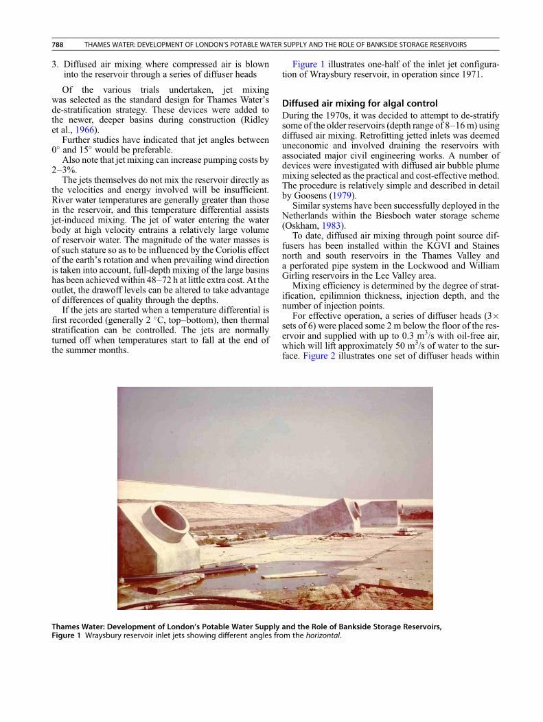
788 THAMES WATER: DEVELOPMENT OF LONDON’S POTABLE WATER SUPPLY AND THE ROLE OF BANKSIDE STORAGE RESERVOIRS

3. Diffused air mixing where compressed air is blowninto the reservoir through a series of diffuser heads

Of the various trials undertaken, jet mixingwas selected as the standard design for Thames Water’sde-stratification strategy. These devices were added tothe newer, deeper basins during construction (Ridleyet al., 1966).

Further studies have indicated that jet angles between0� and 15� would be preferable.

Also note that jet mixing can increase pumping costs by2–3%.

The jets themselves do not mix the reservoir directly asthe velocities and energy involved will be insufficient.River water temperatures are generally greater than thosein the reservoir, and this temperature differential assistsjet-induced mixing. The jet of water entering the waterbody at high velocity entrains a relatively large volumeof reservoir water. The magnitude of the water masses isof such stature so as to be influenced by the Coriolis effectof the earth’s rotation and when prevailing wind directionis taken into account, full-depth mixing of the large basinshas been achievedwithin 48–72 h at little extra cost. At theoutlet, the drawoff levels can be altered to take advantageof differences of quality through the depths.

If the jets are started when a temperature differential isfirst recorded (generally 2 �C, top–bottom), then thermalstratification can be controlled. The jets are normallyturned off when temperatures start to fall at the end ofthe summer months.

Thames Water: Development of London’s Potable Water SupplyFigure 1 Wraysbury reservoir inlet jets showing different angles fro

Figure 1 illustrates one-half of the inlet jet configura-tion of Wraysbury reservoir, in operation since 1971.

Diffused air mixing for algal controlDuring the 1970s, it was decided to attempt to de-stratifysome of the older reservoirs (depth range of 8–16m) usingdiffused air mixing. Retrofitting jetted inlets was deemeduneconomic and involved draining the reservoirs withassociated major civil engineering works. A number ofdevices were investigated with diffused air bubble plumemixing selected as the practical and cost-effective method.The procedure is relatively simple and described in detailby Goosens (1979).

Similar systems have been successfully deployed in theNetherlands within the Biesboch water storage scheme(Oskham, 1983).

To date, diffused air mixing through point source dif-fusers has been installed within the KGVI and Stainesnorth and south reservoirs in the Thames Valley anda perforated pipe system in the Lockwood and WilliamGirling reservoirs in the Lee Valley area.

Mixing efficiency is determined by the degree of strat-ification, epilimnion thickness, injection depth, and thenumber of injection points.

For effective operation, a series of diffuser heads (3�sets of 6) were placed some 2 m below the floor of the res-ervoir and supplied with up to 0.3 m3/s with oil-free air,which will lift approximately 50 m3/s of water to the sur-face. Figure 2 illustrates one set of diffuser heads within

and the Role of Bankside Storage Reservoirs,m the horizontal.

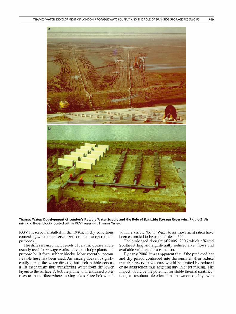
Thames Water: Development of London’s Potable Water Supply and the Role of Bankside Storage Reservoirs, Figure 2 Airmixing diffuser blocks located within KGV1 reservoir, Thames Valley.

THAMES WATER: DEVELOPMENT OF LONDON’S POTABLE WATER SUPPLY AND THE ROLE OF BANKSIDE STORAGE RESERVOIRS 789

KGV1 reservoir installed in the 1980s, in dry conditionscoinciding when the reservoir was drained for operationalpurposes.

The diffusers used include sets of ceramic domes, moreusually used for sewage works activated sludge plants andpurpose built foam rubber blocks. More recently, porousflexible hose has been used. Air mixing does not signifi-cantly aerate the water directly, but each bubble acts asa lift mechanism thus transferring water from the lowerlayers to the surface. A bubble plume with entrained waterrises to the surface where mixing takes place below and

within a visible “boil.”Water to air movement ratios havebeen estimated to be in the order 1:240.

The prolonged drought of 2005–2006 which affectedSoutheast England significantly reduced river flows andavailable volumes for abstraction.

By early 2006, it was apparent that if the predicted hotand dry period continued into the summer, then reducetreatable reservoir volumes would be limited by reducedor no abstraction thus negating any inlet jet mixing. Theimpact would be the potential for stable thermal stratifica-tion, a resultant deterioration in water quality with

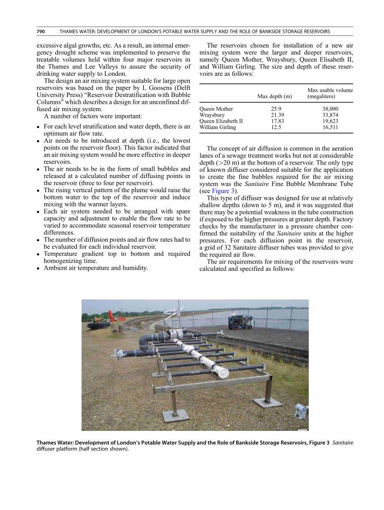
790 THAMES WATER: DEVELOPMENT OF LONDON’S POTABLE WATER SUPPLY AND THE ROLE OF BANKSIDE STORAGE RESERVOIRS

excessive algal growths, etc. As a result, an internal emer-gency drought scheme was implemented to preserve thetreatable volumes held within four major reservoirs inthe Thames and Lee Valleys to assure the security ofdrinking water supply to London.

The design an air mixing system suitable for large openreservoirs was based on the paper by L Goosens (DelftUniversity Press) “Reservoir Destratification with BubbleColumns”which describes a design for an unconfined dif-fused air mixing system.

A number of factors were important:

� For each level stratification and water depth, there is anoptimum air flow rate.

� Air needs to be introduced at depth (i.e., the lowestpoints on the reservoir floor). This factor indicated thatan air mixing system would be more effective in deeperreservoirs.

� The air needs to be in the form of small bubbles andreleased at a calculated number of diffusing points inthe reservoir (three to four per reservoir).

� The rising vertical pattern of the plume would raise thebottom water to the top of the reservoir and inducemixing with the warmer layers.

� Each air system needed to be arranged with sparecapacity and adjustment to enable the flow rate to bevaried to accommodate seasonal reservoir temperaturedifferences.

� The number of diffusion points and air flow rates had tobe evaluated for each individual reservoir.

� Temperature gradient top to bottom and requiredhomogenizing time.

� Ambient air temperature and humidity.

Thames Water: Development of London’s Potable Water Supply adiffuser platform (half section shown).

The reservoirs chosen for installation of a new airmixing system were the larger and deeper reservoirs,namely Queen Mother, Wraysbury, Queen Elisabeth II,and William Girling. The size and depth of these reser-voirs are as follows:

nd the Role of Bankside

Max depth (m)

Storage Reservoirs

Max usable volume(megaliters)

Queen Mother 25.9 38,000

Wraysbury 21.39 33,874 Queen Elizabeth II 17.83 19,623 William Girling 12.5 16,511

The concept of air diffusion is common in the aerationlanes of a sewage treatment works but not at considerabledepth (>20 m) at the bottom of a reservoir. The only typeof known diffuser considered suitable for the applicationto create the fine bubbles required for the air mixingsystem was the Sanitaire Fine Bubble Membrane Tube(see Figure 3).

This type of diffuser was designed for use at relativelyshallow depths (down to 5 m), and it was suggested thatthere may be a potential weakness in the tube constructionif exposed to the higher pressures at greater depth. Factorychecks by the manufacturer in a pressure chamber con-firmed the suitability of the Sanitaire units at the higherpressures. For each diffusion point in the reservoir,a grid of 32 Sanitaire diffuser tubes was provided to givethe required air flow.

The air requirements for mixing of the reservoirs werecalculated and specified as follows:

, Figure 3 Sanitaire

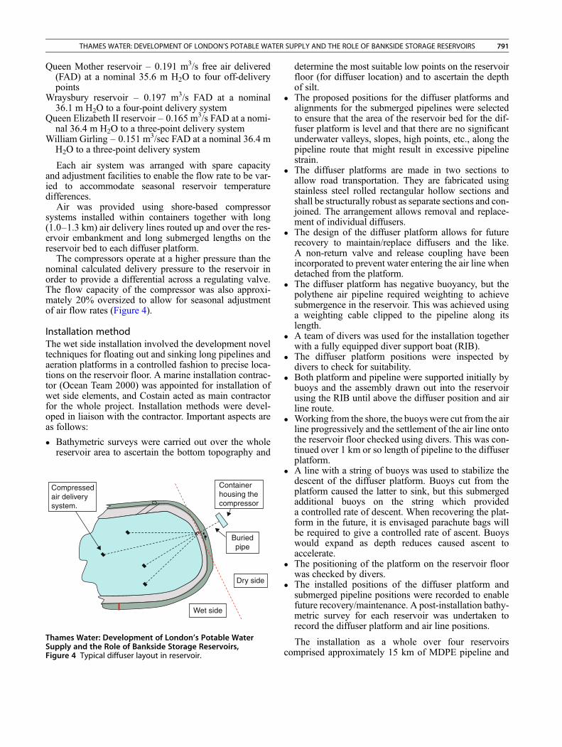
THAMES WATER: DEVELOPMENT OF LONDON’S POTABLE WATER SUPPLY AND THE ROLE OF BANKSIDE STORAGE RESERVOIRS 791

Queen Mother reservoir – 0.191 m3/s free air delivered(FAD) at a nominal 35.6 m H2O to four off-deliverypoints

Wraysbury reservoir – 0.197 m3/s FAD at a nominal36.1 m H2O to a four-point delivery system

Queen Elizabeth II reservoir – 0.165 m3/s FAD at a nomi-nal 36.4 m H2O to a three-point delivery system

William Girling – 0.151 m3/sec FAD at a nominal 36.4 mH2O to a three-point delivery system

Each air system was arranged with spare capacityand adjustment facilities to enable the flow rate to be var-ied to accommodate seasonal reservoir temperaturedifferences.

Air was provided using shore-based compressorsystems installed within containers together with long(1.0–1.3 km) air delivery lines routed up and over the res-ervoir embankment and long submerged lengths on thereservoir bed to each diffuser platform.

The compressors operate at a higher pressure than thenominal calculated delivery pressure to the reservoir inorder to provide a differential across a regulating valve.The flow capacity of the compressor was also approxi-mately 20% oversized to allow for seasonal adjustmentof air flow rates (Figure 4).

Installation methodThe wet side installation involved the development noveltechniques for floating out and sinking long pipelines andaeration platforms in a controlled fashion to precise loca-tions on the reservoir floor. A marine installation contrac-tor (Ocean Team 2000) was appointed for installation ofwet side elements, and Costain acted as main contractorfor the whole project. Installation methods were devel-oped in liaison with the contractor. Important aspects areas follows:

� Bathymetric surveys were carried out over the wholereservoir area to ascertain the bottom topography and

Wet side

Dry side

Buriedpipe

Containerhousing thecompressor

Compressedair deliverysystem.

Thames Water: Development of London’s Potable WaterSupply and the Role of Bankside Storage Reservoirs,Figure 4 Typical diffuser layout in reservoir.

determine the most suitable low points on the reservoirfloor (for diffuser location) and to ascertain the depthof silt.

� The proposed positions for the diffuser platforms andalignments for the submerged pipelines were selectedto ensure that the area of the reservoir bed for the dif-fuser platform is level and that there are no significantunderwater valleys, slopes, high points, etc., along thepipeline route that might result in excessive pipelinestrain.

� The diffuser platforms are made in two sections toallow road transportation. They are fabricated usingstainless steel rolled rectangular hollow sections andshall be structurally robust as separate sections and con-joined. The arrangement allows removal and replace-ment of individual diffusers.

� The design of the diffuser platform allows for futurerecovery to maintain/replace diffusers and the like.A non-return valve and release coupling have beenincorporated to prevent water entering the air line whendetached from the platform.

� The diffuser platform has negative buoyancy, but thepolythene air pipeline required weighting to achievesubmergence in the reservoir. This was achieved usinga weighting cable clipped to the pipeline along itslength.

� A team of divers was used for the installation togetherwith a fully equipped diver support boat (RIB).

� The diffuser platform positions were inspected bydivers to check for suitability.

� Both platform and pipeline were supported initially bybuoys and the assembly drawn out into the reservoirusing the RIB until above the diffuser position and airline route.

� Working from the shore, the buoys were cut from the airline progressively and the settlement of the air line ontothe reservoir floor checked using divers. This was con-tinued over 1 km or so length of pipeline to the diffuserplatform.

� A line with a string of buoys was used to stabilize thedescent of the diffuser platform. Buoys cut from theplatform caused the latter to sink, but this submergedadditional buoys on the string which provideda controlled rate of descent. When recovering the plat-form in the future, it is envisaged parachute bags willbe required to give a controlled rate of ascent. Buoyswould expand as depth reduces caused ascent toaccelerate.

� The positioning of the platform on the reservoir floorwas checked by divers.

� The installed positions of the diffuser platform andsubmerged pipeline positions were recorded to enablefuture recovery/maintenance. A post-installation bathy-metric survey for each reservoir was undertaken torecord the diffuser platform and air line positions.

The installation as a whole over four reservoirscomprised approximately 15 km of MDPE pipeline and

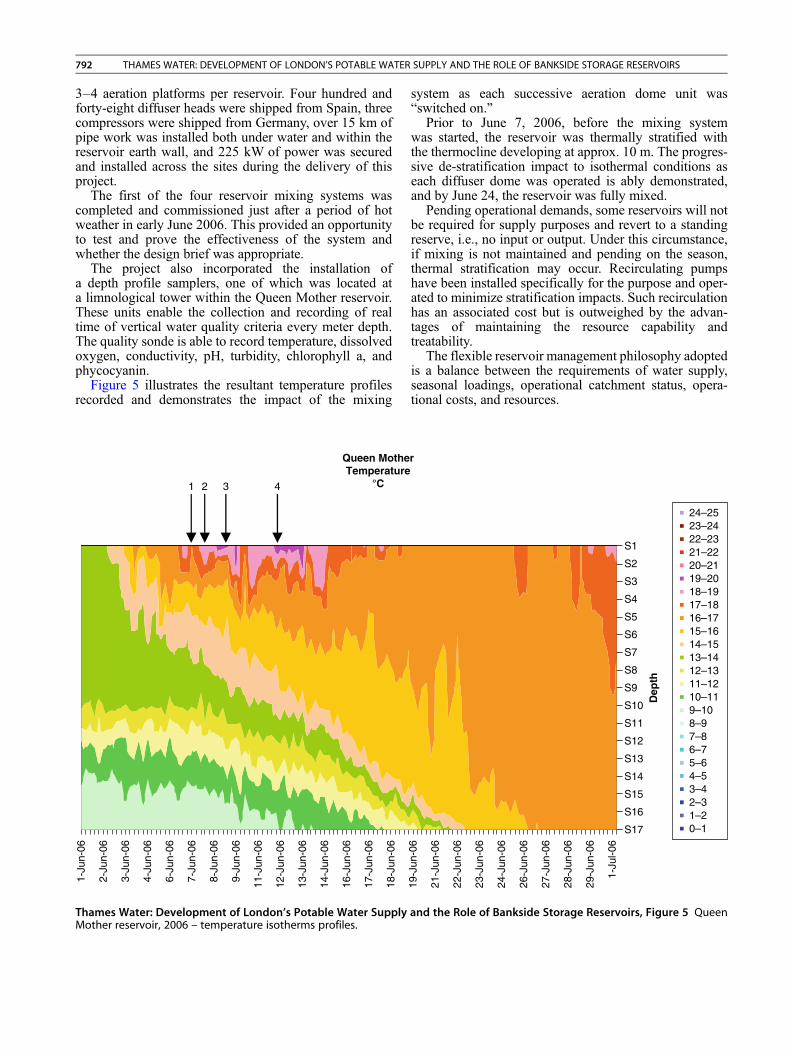
792 THAMES WATER: DEVELOPMENT OF LONDON’S POTABLE WATER SUPPLY AND THE ROLE OF BANKSIDE STORAGE RESERVOIRS

3–4 aeration platforms per reservoir. Four hundred andforty-eight diffuser heads were shipped from Spain, threecompressors were shipped from Germany, over 15 km ofpipe work was installed both under water and within thereservoir earth wall, and 225 kW of power was securedand installed across the sites during the delivery of thisproject.

The first of the four reservoir mixing systems wascompleted and commissioned just after a period of hotweather in early June 2006. This provided an opportunityto test and prove the effectiveness of the system andwhether the design brief was appropriate.

The project also incorporated the installation ofa depth profile samplers, one of which was located ata limnological tower within the Queen Mother reservoir.These units enable the collection and recording of realtime of vertical water quality criteria every meter depth.The quality sonde is able to record temperature, dissolvedoxygen, conductivity, pH, turbidity, chlorophyll a, andphycocyanin.

Figure 5 illustrates the resultant temperature profilesrecorded and demonstrates the impact of the mixing

1-Ju

n-06

2-Ju

n-06

3-Ju

n-06

4-Ju

n-06

6-Ju

n-06

7-Ju

n-06

8-Ju

n-06

9-Ju

n-06

11-J

un-0

6

12-J

un-0

6

13-J

un-0

6

14-J

un-0

6

16-J

un-0

6

17-J

un-0

6

18-J

un-0

6

Queen MotheTemperature

°C1 42 3

Thames Water: Development of London’s Potable Water SupplyMother reservoir, 2006 – temperature isotherms profiles.

system as each successive aeration dome unit was“switched on.”

Prior to June 7, 2006, before the mixing systemwas started, the reservoir was thermally stratified withthe thermocline developing at approx. 10 m. The progres-sive de-stratification impact to isothermal conditions aseach diffuser dome was operated is ably demonstrated,and by June 24, the reservoir was fully mixed.

Pending operational demands, some reservoirs will notbe required for supply purposes and revert to a standingreserve, i.e., no input or output. Under this circumstance,if mixing is not maintained and pending on the season,thermal stratification may occur. Recirculating pumpshave been installed specifically for the purpose and oper-ated to minimize stratification impacts. Such recirculationhas an associated cost but is outweighed by the advan-tages of maintaining the resource capability andtreatability.

The flexible reservoir management philosophy adoptedis a balance between the requirements of water supply,seasonal loadings, operational catchment status, opera-tional costs, and resources.

19-J

un-0

6

21-J

un-0

6

22-J

un-0

6

23-J

un-0

6

24-J

un-0

6

26-J

un-0

6

27-J

un-0

6

28-J

un-0

6

29-J

un-0

6

1-Ju

l-06

S1

S2

S3

S4

S5

S6

S7

S8

S9

S10

S11

S12

S13

S14

S15

S16

S17

Dep

th

r

24–2523–2422–2321–2220–2119–2018–1917–1816–1715–1614–1513–1412–1311–1210–119–108–97–86–75–64–53–42–31–20–1

and the Role of Bankside Storage Reservoirs, Figure 5 Queen

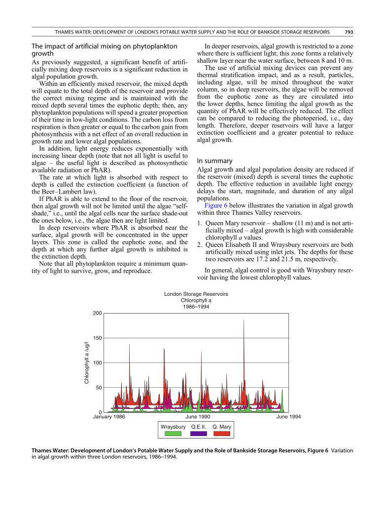
THAMES WATER: DEVELOPMENT OF LONDON’S POTABLE WATER SUPPLY AND THE ROLE OF BANKSIDE STORAGE RESERVOIRS 793

The impact of artificial mixing on phytoplanktongrowthAs previously suggested, a significant benefit of artifi-cially mixing deep reservoirs is a significant reduction inalgal population growth.

Within an efficiently mixed reservoir, the mixed depthwill equate to the total depth of the reservoir and providethe correct mixing regime and is maintained with themixed depth several times the euphotic depth; then, anyphytoplankton populations will spend a greater proportionof their time in low-light conditions. The carbon loss fromrespiration is then greater or equal to the carbon gain fromphotosynthesis with a net effect of an overall reduction ingrowth rate and lower algal populations.

In addition, light energy reduces exponentially withincreasing linear depth (note that not all light is useful toalgae – the useful light is described as photosyntheticavailable radiation or PhAR).

The rate at which light is absorbed with respect todepth is called the extinction coefficient (a function ofthe Beer–Lambert law).

If PhAR is able to extend to the floor of the reservoir,then algal growth will not be limited until the algae “self-shade,” i.e., until the algal cells near the surface shade-outthe ones below, i.e., the algae then are light limited.

In deep reservoirs where PhAR is absorbed near thesurface, algal growth will be concentrated in the upperlayers. This zone is called the euphotic zone, and thedepth at which any further algal growth is inhibited isthe extinction depth.

Note that all phytoplankton require a minimum quan-tity of light to survive, grow, and reproduce.

London StoraChloro1986–

January 19860

50

100

150

200

Wraysbury Q.

June

Chl

orop

hyll

a /u

g/l

ThamesWater: Development of London’s PotableWater Supply ain algal growth within three London reservoirs, 1986–1994.

In deeper reservoirs, algal growth is restricted to a zonewhere there is sufficient light; this zone forms a relativelyshallow layer near the water surface, between 8 and 10 m.

The use of artificial mixing devices can prevent anythermal stratification impact, and as a result, particles,including algae, will be mixed throughout the watercolumn, so in deep reservoirs, the algae will be removedfrom the euphotic zone as they are circulated intothe lower depths, hence limiting the algal growth as thequantity of PhAR will be effectively reduced. The effectcan be compared to reducing the photoperiod, i.e., daylength. Therefore, deeper reservoirs will have a largerextinction coefficient and a greater potential to reducealgal growth.

In summaryAlgal growth and algal population density are reduced ifthe reservoir (mixed) depth is several times the euphoticdepth. The effective reduction in available light energydelays the start, magnitude, and duration of any algalpopulations.

Figure 6 below illustrates the variation in algal growthwithin three Thames Valley reservoirs.

1. Queen Mary reservoir – shallow (11 m) and is not arti-ficially mixed – algal growth is high with considerablechlorophyll a values.

2. Queen Elisabeth II and Wraysbury reservoirs are bothartificially mixed using inlet jets. The depths for thesetwo reservoirs are 17.2 and 21.5 m, respectively.

In general, algal control is good with Wraysbury reser-voir having the lowest chlorophyll values.

ge Reservoirsphyll a1994

June 1994

E.II. Q. Mary

1990

nd the Role of Bankside Storage Reservoirs, Figure 6 Variation

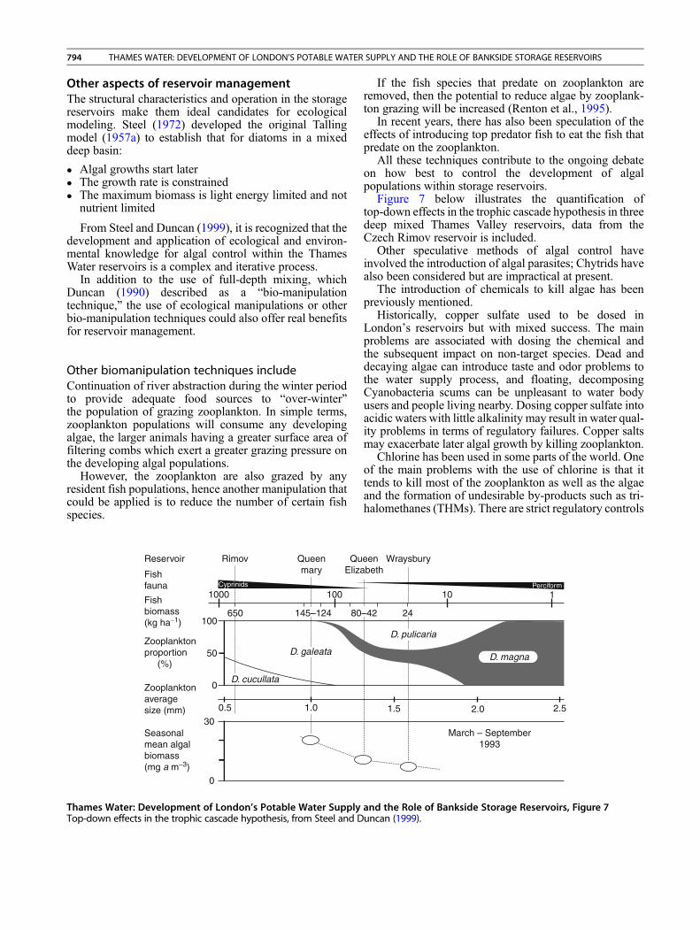
794 THAMES WATER: DEVELOPMENT OF LONDON’S POTABLE WATER SUPPLY AND THE ROLE OF BANKSIDE STORAGE RESERVOIRS

Other aspects of reservoir managementThe structural characteristics and operation in the storagereservoirs make them ideal candidates for ecologicalmodeling. Steel (1972) developed the original Tallingmodel (1957a) to establish that for diatoms in a mixeddeep basin:

� Algal growths start later� The growth rate is constrained� The maximum biomass is light energy limited and not

nutrient limited

From Steel and Duncan (1999), it is recognized that thedevelopment and application of ecological and environ-mental knowledge for algal control within the ThamesWater reservoirs is a complex and iterative process.

In addition to the use of full-depth mixing, whichDuncan (1990) described as a “bio-manipulationtechnique,” the use of ecological manipulations or otherbio-manipulation techniques could also offer real benefitsfor reservoir management.

Other biomanipulation techniques includeContinuation of river abstraction during the winter periodto provide adequate food sources to “over-winter”the population of grazing zooplankton. In simple terms,zooplankton populations will consume any developingalgae, the larger animals having a greater surface area offiltering combs which exert a greater grazing pressure onthe developing algal populations.

However, the zooplankton are also grazed by anyresident fish populations, hence another manipulation thatcould be applied is to reduce the number of certain fishspecies.

Reservoir Rimov

1000

650100

50

0.5

30

0

1.0

D. cucullata

D. galeata

0

145–124 80

100Cyprinids

Queenmary

QuElizaFish

fauna

Fishbiomass(kg ha−1)

Zooplanktonaveragesize (mm)

Seasonalmean algalbiomass(mg a m−3)

Zooplanktonproportion (%)

Thames Water: Development of London’s Potable Water SupplyTop-down effects in the trophic cascade hypothesis, from Steel and D

If the fish species that predate on zooplankton areremoved, then the potential to reduce algae by zooplank-ton grazing will be increased (Renton et al., 1995).

In recent years, there has also been speculation of theeffects of introducing top predator fish to eat the fish thatpredate on the zooplankton.

All these techniques contribute to the ongoing debateon how best to control the development of algalpopulations within storage reservoirs.

Figure 7 below illustrates the quantification oftop-down effects in the trophic cascade hypothesis in threedeep mixed Thames Valley reservoirs, data from theCzech Rimov reservoir is included.

Other speculative methods of algal control haveinvolved the introduction of algal parasites; Chytrids havealso been considered but are impractical at present.

The introduction of chemicals to kill algae has beenpreviously mentioned.

Historically, copper sulfate used to be dosed inLondon’s reservoirs but with mixed success. The mainproblems are associated with dosing the chemical andthe subsequent impact on non-target species. Dead anddecaying algae can introduce taste and odor problems tothe water supply process, and floating, decomposingCyanobacteria scums can be unpleasant to water bodyusers and people living nearby. Dosing copper sulfate intoacidic waters with little alkalinity may result in water qual-ity problems in terms of regulatory failures. Copper saltsmay exacerbate later algal growth by killing zooplankton.

Chlorine has been used in some parts of the world. Oneof the main problems with the use of chlorine is that ittends to kill most of the zooplankton as well as the algaeand the formation of undesirable by-products such as tri-halomethanes (THMs). There are strict regulatory controls

1.5 2.0

March – September1993

2.5

D. pulicaria

–42 24

10Perciform

1

eenbeth

Wraysbury

D. magna

and the Role of Bankside Storage Reservoirs, Figure 7uncan (1999).

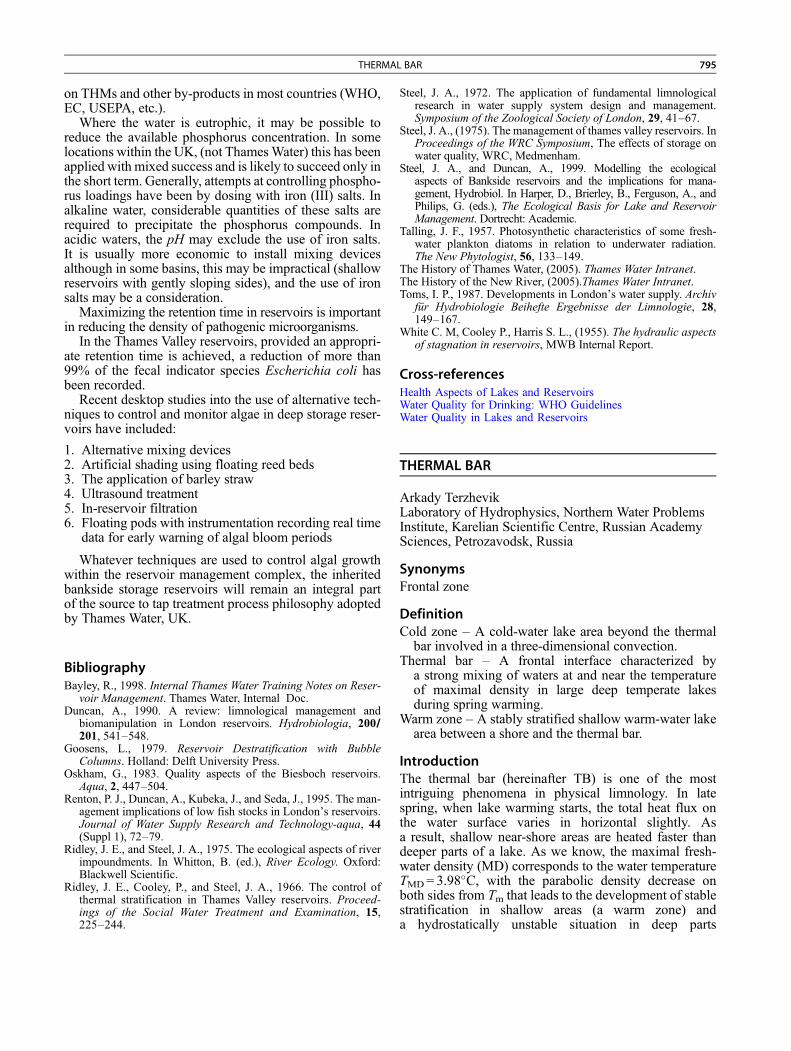
THERMAL BAR 795

on THMs and other by-products in most countries (WHO,EC, USEPA, etc.).

Where the water is eutrophic, it may be possible toreduce the available phosphorus concentration. In somelocations within the UK, (not ThamesWater) this has beenapplied with mixed success and is likely to succeed only inthe short term. Generally, attempts at controlling phospho-rus loadings have been by dosing with iron (III) salts. Inalkaline water, considerable quantities of these salts arerequired to precipitate the phosphorus compounds. Inacidic waters, the pH may exclude the use of iron salts.It is usually more economic to install mixing devicesalthough in some basins, this may be impractical (shallowreservoirs with gently sloping sides), and the use of ironsalts may be a consideration.

Maximizing the retention time in reservoirs is importantin reducing the density of pathogenic microorganisms.

In the Thames Valley reservoirs, provided an appropri-ate retention time is achieved, a reduction of more than99% of the fecal indicator species Escherichia coli hasbeen recorded.

Recent desktop studies into the use of alternative tech-niques to control and monitor algae in deep storage reser-voirs have included:

1. Alternative mixing devices2. Artificial shading using floating reed beds3. The application of barley straw4. Ultrasound treatment5. In-reservoir filtration6. Floating pods with instrumentation recording real time

data for early warning of algal bloom periods

Whatever techniques are used to control algal growthwithin the reservoir management complex, the inheritedbankside storage reservoirs will remain an integral partof the source to tap treatment process philosophy adoptedby Thames Water, UK.

BibliographyBayley, R., 1998. Internal Thames Water Training Notes on Reser-

voir Management. Thames Water, Internal Doc.Duncan, A., 1990. A review: limnological management and

biomanipulation in London reservoirs. Hydrobiologia, 200/201, 541–548.

Goosens, L., 1979. Reservoir Destratification with BubbleColumns. Holland: Delft University Press.

Oskham, G., 1983. Quality aspects of the Biesboch reservoirs.Aqua, 2, 447–504.

Renton, P. J., Duncan, A., Kubeka, J., and Seda, J., 1995. The man-agement implications of low fish stocks in London’s reservoirs.Journal of Water Supply Research and Technology-aqua, 44(Suppl 1), 72–79.

Ridley, J. E., and Steel, J. A., 1975. The ecological aspects of riverimpoundments. In Whitton, B. (ed.), River Ecology. Oxford:Blackwell Scientific.

Ridley, J. E., Cooley, P., and Steel, J. A., 1966. The control ofthermal stratification in Thames Valley reservoirs. Proceed-ings of the Social Water Treatment and Examination, 15,225–244.

Steel, J. A., 1972. The application of fundamental limnologicalresearch in water supply system design and management.Symposium of the Zoological Society of London, 29, 41–67.

Steel, J. A., (1975). The management of thames valley reservoirs. InProceedings of the WRC Symposium, The effects of storage onwater quality, WRC, Medmenham.

Steel, J. A., and Duncan, A., 1999. Modelling the ecologicalaspects of Bankside reservoirs and the implications for mana-gement, Hydrobiol. In Harper, D., Brierley, B., Ferguson, A., andPhilips, G. (eds.), The Ecological Basis for Lake and ReservoirManagement. Dortrecht: Academic.

Talling, J. F., 1957. Photosynthetic characteristics of some fresh-water plankton diatoms in relation to underwater radiation.The New Phytologist, 56, 133–149.

The History of Thames Water, (2005). Thames Water Intranet.The History of the New River, (2005).Thames Water Intranet.Toms, I. P., 1987. Developments in London’s water supply. Archiv

für Hydrobiologie Beihefte Ergebnisse der Limnologie, 28,149–167.

White C. M, Cooley P., Harris S. L., (1955). The hydraulic aspectsof stagnation in reservoirs, MWB Internal Report.

Cross-referencesHealth Aspects of Lakes and ReservoirsWater Quality for Drinking: WHO GuidelinesWater Quality in Lakes and Reservoirs

THERMAL BAR

Arkady TerzhevikLaboratory of Hydrophysics, Northern Water ProblemsInstitute, Karelian Scientific Centre, Russian AcademySciences, Petrozavodsk, Russia

SynonymsFrontal zone

DefinitionCold zone – A cold-water lake area beyond the thermal

bar involved in a three-dimensional convection.Thermal bar – A frontal interface characterized by

a strong mixing of waters at and near the temperatureof maximal density in large deep temperate lakesduring spring warming.

Warm zone – A stably stratified shallow warm-water lakearea between a shore and the thermal bar.

IntroductionThe thermal bar (hereinafter TB) is one of the mostintriguing phenomena in physical limnology. In latespring, when lake warming starts, the total heat flux onthe water surface varies in horizontal slightly. Asa result, shallow near-shore areas are heated faster thandeeper parts of a lake. As we know, the maximal fresh-water density (MD) corresponds to the water temperatureTMD= 3.98�C, with the parabolic density decrease onboth sides from Tm that leads to the development of stablestratification in shallow areas (a warm zone) anda hydrostatically unstable situation in deep parts

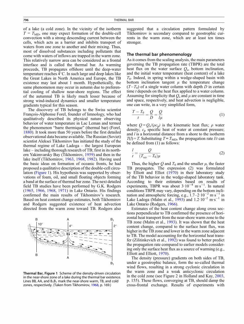
796 THERMAL BAR

of a lake (a cold zone). In the vicinity of the isothermT = TMD, one may expect formation of the double-cellconvection with a strong descending current between thecells, which acts as a barrier and inhibits transport ofwaters from one zone to another and their mixing. Thus,most of dissolved substances including pollutants thatcome with waters of inflows are trapped in the warm zone.This relatively narrow area can be considered as a frontalinterface and is called the thermal bar. As warmingproceeds, TB propagates offshore until the deep-watertemperature reaches 4�C. In such large and deep lakes likethe Great Lakes in North America and Europe, the TBexistence may last about 1 month. Hypothetically, thesame phenomenon may occur in autumn due to preferen-tial cooling of shallow near-shore regions. The effectof the autumnal TB is likely much lesser because ofstrong wind-induced dynamics and smaller temperaturegradients typical for this season.

The discovery of TB belongs to the Swiss scientistFrançois-Alphonse Forel, founder of limnology, who hadqualitatively described its physical nature observingbehavior of water temperature in Lac Leman and termedthe phenomenon “barre thermique” (thermal bar) (Forel,1880). It took more than 50 years before the first detailedobservational data became available. The Russian (Soviet)scientist Aleksei Tikhomirov has initiated the study of thethermal regime of Lake Ladoga – the largest Europeanlake – including thorough research of TB; first in its north-ern Yakimvarsky Bay (Tikhomirov, 1959) and then in thelake itself (Tikhomirov, 1963, 1968, 1982). Having usedthe basic ideas on formation of oceanic fronts, he hadproposed a qualitative description of the double-cell circu-lation (Figure 1). His hypothesis was supported by obser-vations of foam, oil, and small floating objects forminga band at the surface of thermal bar zone. The next detailedfield TB studies have been performed by G.K. Rodgers(1965, 1966, 1968, 1971) in Lake Ontario. His findingsconfirmed the main results of Tikhomirov’s research.Based on heat content change estimates, both Tikhomirovand Rodgers suggested existence of heat advectiondirected from the warm zone toward TB. Rodgers also

10°B

BA

A B1

B1

4° 2°

Thermal Bar, Figure 1 Scheme of the density-driven circulationin the near-shore zone of a lake during the thermal bar existence.Lines BB, AA, and B1B1 mark the near-shore warm, TB, and coldzones, respectively. (Taken from Tikhomirov, 1968, p. 169.)

suggested that a circulation pattern formulated byTikhomirov is secondary compared to geostrophic cur-rents in the warm zone, which are at least ten timesstronger.

The thermal bar phenomenologyAs it comes from the scaling analysis, the main parametersgoverning the TB propagation rate (TBPR) are the totalheat flux on the water surface Qs, bottom inclination,and the initial water temperature (heat content) of a lakeT0. Indeed, in spring within a wedge-shaped basin withbottom inclination tangent m the temperature change(T�T0) of a single water column with depth D in certaintime t depends on the heat flux applied to a water column.Assuming for simplicity thatQs and m are constant in timeand space, respectively, and heat advection is negligible,one can write, in a very simplified form,

T � T0t

¼ QD¼ Q

lm(1)

where Q=Qs/(rcp) is the kinematic heat flux; r waterdensity; cp specific heat of water at constant pressure;and l is a horizontal distance from a shore to the isothermT(l) = T. Substituting T= TMD, the propagation rate l/t canbe defined from (1) as follows:

lt¼ Q

ðTMD � T0Þm (2)

Thus, the higher Q and T and the smaller m, the faster

0TB propagates. The expression (2) was formulatedby Elliott and Elliot (1970) in their laboratory studyof the TB behavior in the wedge-shaped laboratory tank.According to their estimates based on results ofexperiments, TBPR was about 3·10�4 m·s�1. In naturalconditions TBPRmay vary, depending on the bottom incli-nation and atmospheric forcing, e.g., 1.7–2·10�2 m·s�1 inLake Ladoga (Malm et al., 1993) and 1.2·10–2 m·s�1 inLake Ontario (Rodgers, 1966).

Estimates of the heat content change along cross sec-tions perpendicular to TB confirmed the presence of hori-zontal heat transport from the near-shore warm zone to theTB zone (Malm et al., 1993). It was shown that the heatcontent change, compared to the surface heat flux, washigher in the TB zone and lower in the warm zone adjacentto TB. The model accounting for the horizontal heat trans-fer (Zilitinkevich et al., 1992) was found to better predictthe propagation rate compared to earlier models consider-ing only the surface heat flux as a source of warming (e.g.,Elliott and Elliott, 1970).

The density (pressure) gradients on both sides of TB,under a geostrophic balance, form the so-called thermalwind flows, resulting in a strong cyclonic circulation inthe warm zone and a weak anticyclonic circulationin the cold zone (see Figure 2 in Holland and Kay, 2003,p. 155). These flows, converging at TB, should damp thecross-frontal exchange. Results of experiments with

THERMAL REGIME OF LAKES 797

natural tracers have shown that little mixing occursbetween inshore and offshore waters, thus TB can be con-sidered as a barrier separating warm and cold zones(Menon et al., 1971; Hubbard and Spain, 1973; Spainet al., 1976). Later observations (Gbah and Murthy,1998; Rao et al., 2004) revealed that horizontal diffusionacross the TB zone is consistently smaller thanthat directed along the front. The cross-frontal exchangecoefficients are several orders of magnitude smaller thantypical coastal values in the absence of TB.

SummaryThe thermal bar is the unique physical phenomenon thatshould be studied further to better understand its nature,e.g., a clear formulation of the mechanism governing heattransport from the warm zone toward TB. SergeiZilitinkevich (unpublished manuscript) suggested that itmay occur due to baroclinic instability of geostrophic cur-rents in the warm zone. Besides the strong effect on lakehydrodynamics, TB is every bit important from the stand-point of the impact on lake ecosystems, e.g., strongmixingin the TB zone, which leads to the longer life of allsubstances – including nutrients and pollutants – comingwith inflow waters, in the lake proper. This in its turnmay affect the seasonal development of plankton anda number of pollution events. Strong mixing may alsoaccelerate sinking rates of newly formed organic matterand detritus, and then the former should intensify micro-bial activity in the bottom layers.

The limited space does not allow to givea comprehensive state-of-the-art review on TB studiesperformed. To get a better insight into the problem,a curious reader can be referred to the paper by Hollandand Kay (2003). The authors nicely compiled most ofobservational, theoretical, and modeling studies carriedout for the last 50 years, and suggested the outlook forfurther research.

BibliographyElliott, G. H., and Elliott, J. A., 1970. Laboratory studies on the

thermal bar. In Proceedings of 13th Great Lakes Research. Inter-national Association of Great Lakes Research, pp. 413–418.

Forel, F. A., 1880. La congelation des lacs Suisses et savoyardspendant l'hiver 1879–1880, Lac Leman. L'Echo des Alpes, 3,149–161.

Gbah, M. B., and Murthy, R. C., 1998. Characteristics of turbulentcross and alongshore voventum exchanges during a thermalbar episode in Lake Ontario. Nordic Hydrology, 29, 57–72.

Holland, P. R., and Kay, A., 2003. A review on the physics andecological implications of the thermal bar circulation.Limnologica, 33, 153–162.

Hubbard, D. W., and Spain, I. D., 1973. The structure of the earlyspring thermal bar in Lake Superior, I. In Proceedings of 16thConference Great Lakes Research. International Association ofGreat Lakes Research, pp. 735–742

Malm, J., 1995. Spring circulation associated with the thermal bar inlarge temperate lakes. Nordic Hydrology, 26, 331–358.

Malm, J., Mironov, D., Terzhevik, A., and Grahn, L., 1993. FieldInvestigation of the Thermal Bar in Lake Ladoga, Spring 1991.Nordic Hydrology, 24, 339–358.

Menon, A. S., Dutka, B. J., and Jurkovic, A. A., 1971. Preliminarybacteriological studies of the Lake Ontario thermal bar. In Pro-ceedings 14th Conference Great Lakes Research. InternationalAssociation of Great Lakes Research, pp. 59–68.

Rao, Y. R., Skafel, M. G., and Charlton, M. N., 2004. Circulationand turbulent exchange characteristics during the thermal barin Lake Ontario. Limnology and Oceanography, 49, 2190–2200.

Rodgers, G. K., 1965. The thermal bar in the Laurentian GreatLakes. In Proceedings of the 8th Conference on Great LakesResearch. University of Michigan, publ. 13, pp. 358–363.

Rodgers, G. K., 1966. The thermal bar in Lake Ontario, spring 1965and winter 1965–1966. In Proceedings of the 9th Conference onGreat Lakes Research. University of Michigan, publ. 15,pp. 369–374.

Rodgers, G. K., 1968. Heat advection within Lake Ontario inspring and surface water transparency associated with the ther-mal bar. In Proceedings of the 11th Conference on Great LakesResearch. International Association of Great Lakes Research,pp. 942–950.

Rodgers, G. K., 1971. Field investigation on the thermal bar in LakeOntario: precision temperature measurements. In Proceedings ofthe 14th Conference on Great Lakes Research. InternationalAssociation of Great Lakes Research, pp. 618–624.

Spain, J. D., Wernert, G. M., and Hubbard, D. W., 1976. Thestructure of the spring thermal bar in Lake Superior, II. Journalof Great Lakes Research, 2, 296–306.

Tikhomirov, A. I., 1959. The thermal bar in the Yakimvarsky Bay ofLake Ladoga. Izvestiya of All-Union Geographical Society, 91,424–438 (in Russian).

Tikhomirov, A. I., 1963. The thermal bar of Lake Ladoga. Izvestiyaof All-Union Geographical Society, 95, 134–142 (in Russian;English translation: American Geophysical Union Transactions,Soviet Hydrology, Selected Papers, No. 2).

Tikhomirov, A. I., 1968. Temperature and heat contents ofLake Ladoga. In Kalesnik, S. V. (ed.), Thermal Regime LakeLadoga. Leningrad: Leningrad University Press, pp. 144–217(in Russian).

Tikhomirov, A. I., 1982. Thermal Regime of Large Lakes.Leningrad: Publishing House Nauka. (in Russian).

Zilitinkevich, S. S., Kreiman, K. D., and Terzhevik, A. Yu., 1992.Thermal bar. Journal of Fluid Mechanics, 236, 27–42.

Cross-referencesGreat Lake Processes: Thermal Structure, Circulation andTurbulent Diffusion ProcessesLadoga Lake and Onego Lake (Lakes Ladozhskoye andOnezhskoye)Riverine Thermal Bar

THERMAL REGIME OF LAKES

Lars BengtssonDepartment of Water Resources Engineering, LundUniversity, Lund, Sweden

IntroductionHeat is transferred to or lost from lake water throughatmospheric exchange and with in- and outflowing rivers.There is also heat exchange with the bottom sediments.Since the depth varies over the lake, the heat exchangeper unit mass is different in different water columns,which sets the water masses in an unstable condition

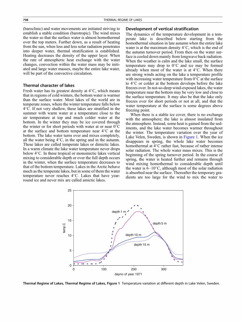
798 THERMAL REGIME OF LAKES

(baroclinic) and water movements are initiated striving toestablish a stable condition (barotropic). The wind mixesthe water so that the surface water is almost homothermalover the top meters. Further down, as a result of heatingfrom the sun, when less and less solar radiation penetratesinto deeper water, thermal stratification is established.Heating decreases the density of the upper layer. Whenthe rate of atmospheric heat exchange with the waterchanges, convection within the water mass may be initi-ated and large water masses, maybe the entire lake water,will be part of the convective circulation.

Thermal character of lakesFresh water has its greatest density at 4�C, which meansthat in regions of cold winters, the bottom water is warmerthan the surface water. Most lakes of the world are intemperate zones, where the winter temperature falls below4�C. If not very shallow, these lakes are stratified in thesummer with warm water at a temperature close to theair temperature at top and much colder water at thebottom. In the winter they may be ice covered throughthe winter or for short periods with water at or near 0�Cat the surface and bottom temperature near 4�C at thebottom. The lake water turns over and mixes completely,all the water being 4�C, in the spring and in the autumn.These lakes are called temperate lakes or dimictic lakes.In a warm climate the lake water temperature never dropsbelow 4�C. In these tropical or monomictic lakes verticalmixing to considerable depth or over the full depth occursin the winter, when the surface temperature decreases tothat of the bottom temperature. Lakes in the Arctic behavemuch as the temperate lakes, but in some of them the watertemperature never reaches 4�C. Lakes that have year-round ice and never mix are called amictic lakes.

0

5

10

15

20

25

0 100

dayno o

tem

p C

depth 1 m

Thermal Regime of Lakes, Thermal Regime of Lakes, Figure 1 Te

Development of vertical stratificationThe dynamics of the temperature development in a tem-perate lake is described below starting from thehomothermal situation in late autumn when the entire lakewater is at the maximum density 4�C, which is the end ofthe autumn turnover period. From then on the water sur-face is cooled downmainly from longwave back radiation.When the weather is calm and the lake small, the surfacetemperature may drop to 0�C and ice may be formedalready when most of the water is at 4�C. When thereare strong winds acting on the lake a temperature profilewith increasing water temperature from 0�C at the surfaceto 4�C or colder at the bottom develops before the lakefreezes over. In not-so-deep wind-exposed lakes, the watertemperature near the bottom may be very low and close tothe surface temperature. It may also be that the lake onlyfreezes over for short periods or not at all, and that thewater temperature at the surface is some degrees abovefreezing point.

When there is a stable ice cover, there is no exchangewith the atmosphere; the lake is almost insulated fromthe atmosphere. Instead, some heat is gained from the sed-iments, and the lake water becomes warmer throughoutthe winter. The temperature variation over the year ofLake Velen, Sweden, is shown in Figure 1. When the icedisappears in spring, the whole lake water becomeshomothermal at 4�C rather fast, because of rather intensesolar radiation. The whole water mass mixes. This is thebeginning of the spring turnover period. In the course ofspring, the water is heated further and remains throughwind mixing homothermal to considerable depth untilthe water is 6–10�C, although most of the solar radiationis absorbed near the surface. Thereafter the temporary gra-dients are too large for the wind to mix the water to

200 300

f year 1971

depth 5 m

depth 15 m

depth 10 m

mperature variation at different depth in Lake Velen, Sweden.

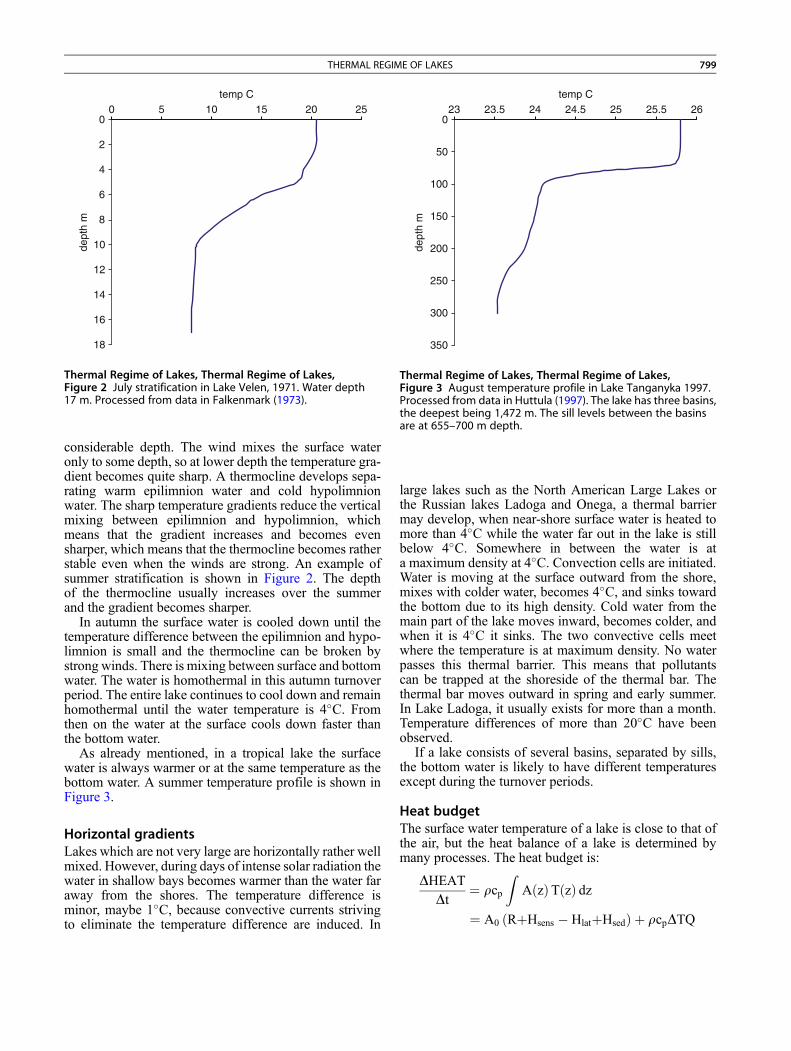
0

50

100

150

200

250

300

350

23 23.5 24.5 25.524 25 26temp C

dept

h m

Thermal Regime of Lakes, Thermal Regime of Lakes,Figure 3 August temperature profile in Lake Tanganyka 1997.Processed from data in Huttula (1997). The lake has three basins,the deepest being 1,472 m. The sill levels between the basinsare at 655–700 m depth.

0

2

4

6

8

10

12

14

16

18

0 5 10 15 20 25temp C

dept

h m

Thermal Regime of Lakes, Thermal Regime of Lakes,Figure 2 July stratification in Lake Velen, 1971. Water depth17 m. Processed from data in Falkenmark (1973).

THERMAL REGIME OF LAKES 799

considerable depth. The wind mixes the surface wateronly to some depth, so at lower depth the temperature gra-dient becomes quite sharp. A thermocline develops sepa-rating warm epilimnion water and cold hypolimnionwater. The sharp temperature gradients reduce the verticalmixing between epilimnion and hypolimnion, whichmeans that the gradient increases and becomes evensharper, which means that the thermocline becomes ratherstable even when the winds are strong. An example ofsummer stratification is shown in Figure 2. The depthof the thermocline usually increases over the summerand the gradient becomes sharper.

In autumn the surface water is cooled down until thetemperature difference between the epilimnion and hypo-limnion is small and the thermocline can be broken bystrong winds. There is mixing between surface and bottomwater. The water is homothermal in this autumn turnoverperiod. The entire lake continues to cool down and remainhomothermal until the water temperature is 4�C. Fromthen on the water at the surface cools down faster thanthe bottom water.

As already mentioned, in a tropical lake the surfacewater is always warmer or at the same temperature as thebottom water. A summer temperature profile is shown inFigure 3.

Horizontal gradientsLakes which are not very large are horizontally rather wellmixed. However, during days of intense solar radiation thewater in shallow bays becomes warmer than the water faraway from the shores. The temperature difference isminor, maybe 1�C, because convective currents strivingto eliminate the temperature difference are induced. In

large lakes such as the North American Large Lakes orthe Russian lakes Ladoga and Onega, a thermal barriermay develop, when near-shore surface water is heated tomore than 4�C while the water far out in the lake is stillbelow 4�C. Somewhere in between the water is ata maximum density at 4�C. Convection cells are initiated.Water is moving at the surface outward from the shore,mixes with colder water, becomes 4�C, and sinks towardthe bottom due to its high density. Cold water from themain part of the lake moves inward, becomes colder, andwhen it is 4�C it sinks. The two convective cells meetwhere the temperature is at maximum density. No waterpasses this thermal barrier. This means that pollutantscan be trapped at the shoreside of the thermal bar. Thethermal bar moves outward in spring and early summer.In Lake Ladoga, it usually exists for more than a month.Temperature differences of more than 20�C have beenobserved.

If a lake consists of several basins, separated by sills,the bottom water is likely to have different temperaturesexcept during the turnover periods.

Heat budgetThe surface water temperature of a lake is close to that ofthe air, but the heat balance of a lake is determined bymany processes. The heat budget is:

DHEATDt

¼ rcp

ZAðzÞTðzÞ dz

¼ A0 ðRþHsens � HlatþHsedÞ þ rcpDTQ

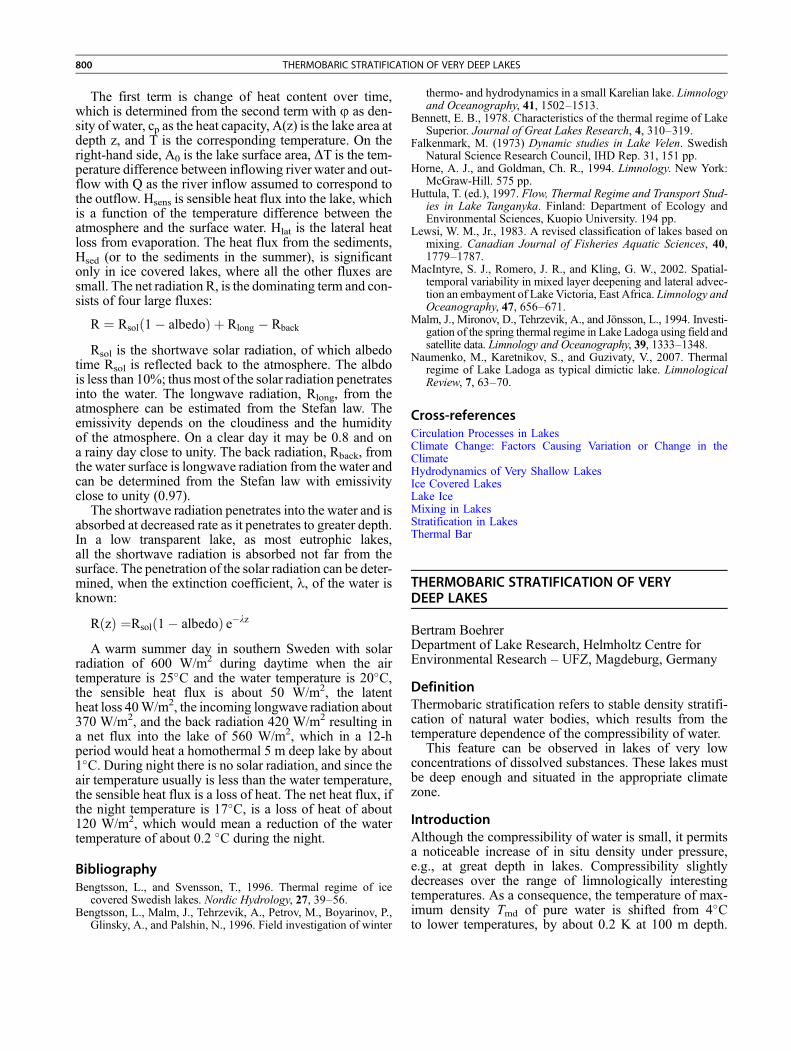
800 THERMOBARIC STRATIFICATION OF VERY DEEP LAKES

The first term is change of heat content over time,

which is determined from the second term with j as den-sity of water, cp as the heat capacity, A(z) is the lake area atdepth z, and T is the corresponding temperature. On theright-hand side, A0 is the lake surface area, DT is the tem-perature difference between inflowing river water and out-flow with Q as the river inflow assumed to correspond tothe outflow. Hsens is sensible heat flux into the lake, whichis a function of the temperature difference between theatmosphere and the surface water. Hlat is the lateral heatloss from evaporation. The heat flux from the sediments,Hsed (or to the sediments in the summer), is significantonly in ice covered lakes, where all the other fluxes aresmall. The net radiation R, is the dominating term and con-sists of four large fluxes:

R ¼ Rsolð1� albedoÞ þ Rlong � Rback

R is the shortwave solar radiation, of which albedo

soltime Rsol is reflected back to the atmosphere. The albdois less than 10%; thusmost of the solar radiation penetratesinto the water. The longwave radiation, Rlong, from theatmosphere can be estimated from the Stefan law. Theemissivity depends on the cloudiness and the humidityof the atmosphere. On a clear day it may be 0.8 and ona rainy day close to unity. The back radiation, Rback, fromthe water surface is longwave radiation from the water andcan be determined from the Stefan law with emissivityclose to unity (0.97).

The shortwave radiation penetrates into the water and isabsorbed at decreased rate as it penetrates to greater depth.In a low transparent lake, as most eutrophic lakes,all the shortwave radiation is absorbed not far from thesurface. The penetration of the solar radiation can be deter-mined, when the extinction coefficient, l, of the water isknown:

RðzÞ ¼Rsolð1� albedoÞ e�lz

A warm summer day in southern Sweden with solar

radiation of 600 W/m2 during daytime when the airtemperature is 25�C and the water temperature is 20�C,the sensible heat flux is about 50 W/m2, the latentheat loss 40W/m2, the incoming longwave radiation about370 W/m2, and the back radiation 420 W/m2 resulting ina net flux into the lake of 560 W/m2, which in a 12-hperiod would heat a homothermal 5 m deep lake by about1�C. During night there is no solar radiation, and since theair temperature usually is less than the water temperature,the sensible heat flux is a loss of heat. The net heat flux, ifthe night temperature is 17�C, is a loss of heat of about120 W/m2, which would mean a reduction of the watertemperature of about 0.2 �C during the night.

BibliographyBengtsson, L., and Svensson, T., 1996. Thermal regime of ice

covered Swedish lakes. Nordic Hydrology, 27, 39–56.Bengtsson, L., Malm, J., Tehrzevik, A., Petrov, M., Boyarinov, P.,

Glinsky, A., and Palshin, N., 1996. Field investigation of winter

thermo- and hydrodynamics in a small Karelian lake. Limnologyand Oceanography, 41, 1502–1513.

Bennett, E. B., 1978. Characteristics of the thermal regime of LakeSuperior. Journal of Great Lakes Research, 4, 310–319.

Falkenmark, M. (1973) Dynamic studies in Lake Velen. SwedishNatural Science Research Council, IHD Rep. 31, 151 pp.

Horne, A. J., and Goldman, Ch. R., 1994. Limnology. New York:McGraw-Hill. 575 pp.

Huttula, T. (ed.), 1997. Flow, Thermal Regime and Transport Stud-ies in Lake Tanganyka. Finland: Department of Ecology andEnvironmental Sciences, Kuopio University. 194 pp.

Lewsi, W. M., Jr., 1983. A revised classification of lakes based onmixing. Canadian Journal of Fisheries Aquatic Sciences, 40,1779–1787.

MacIntyre, S. J., Romero, J. R., and Kling, G. W., 2002. Spatial-temporal variability in mixed layer deepening and lateral advec-tion an embayment of Lake Victoria, East Africa. Limnology andOceanography, 47, 656–671.

Malm, J., Mironov, D., Tehrzevik, A., and Jönsson, L., 1994. Investi-gation of the spring thermal regime in Lake Ladoga using field andsatellite data. Limnology and Oceanography, 39, 1333–1348.

Naumenko, M., Karetnikov, S., and Guzivaty, V., 2007. Thermalregime of Lake Ladoga as typical dimictic lake. LimnologicalReview, 7, 63–70.

Cross-referencesCirculation Processes in LakesClimate Change: Factors Causing Variation or Change in theClimateHydrodynamics of Very Shallow LakesIce Covered LakesLake IceMixing in LakesStratification in LakesThermal Bar

THERMOBARIC STRATIFICATION OF VERYDEEP LAKES

Bertram BoehrerDepartment of Lake Research, Helmholtz Centre forEnvironmental Research – UFZ, Magdeburg, Germany

DefinitionThermobaric stratification refers to stable density stratifi-cation of natural water bodies, which results from thetemperature dependence of the compressibility of water.

This feature can be observed in lakes of very lowconcentrations of dissolved substances. These lakes mustbe deep enough and situated in the appropriate climatezone.

IntroductionAlthough the compressibility of water is small, it permitsa noticeable increase of in situ density under pressure,e.g., at great depth in lakes. Compressibility slightlydecreases over the range of limnologically interestingtemperatures. As a consequence, the temperature of max-imum density Tmd of pure water is shifted from 4�Cto lower temperatures, by about 0.2 K at 100 m depth.

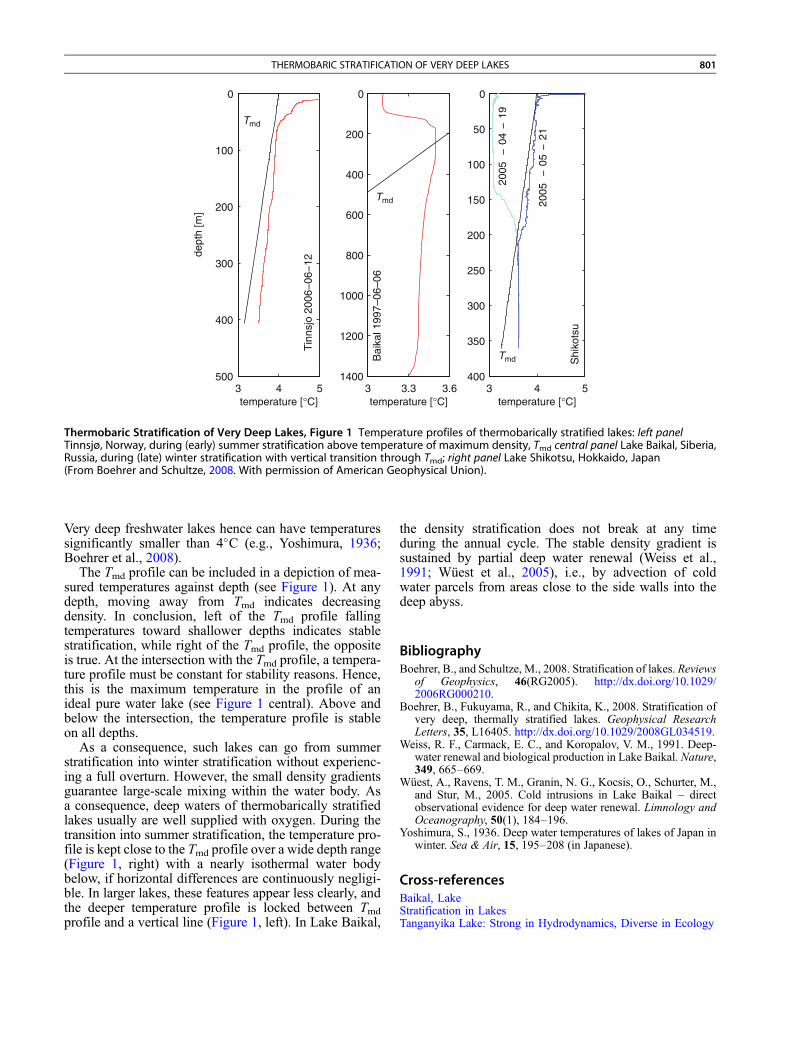
3 4 5500

400

300

200

100

0

Tin

nsjo

200

6−06

−12

dept

h [m

]

3 3.3 3.61400

1200

1000

800

600

400

200

0

3 4 5400

350

300

250

200

150

100

50

0

temperature [°C]temperature [°C]temperature [°C]

Tmd

Tmd

Tmd Shi

kots

u

Bai

kal 1

997–

06–0

6

2005

−04

−19

2005

−05

−21

Thermobaric Stratification of Very Deep Lakes, Figure 1 Temperature profiles of thermobarically stratified lakes: left panelTinnsjø, Norway, during (early) summer stratification above temperature of maximum density, Tmd central panel Lake Baikal, Siberia,Russia, during (late) winter stratification with vertical transition through Tmd; right panel Lake Shikotsu, Hokkaido, Japan(From Boehrer and Schultze, 2008. With permission of American Geophysical Union).

THERMOBARIC STRATIFICATION OF VERY DEEP LAKES 801

Very deep freshwater lakes hence can have temperaturessignificantly smaller than 4�C (e.g., Yoshimura, 1936;Boehrer et al., 2008).

The Tmd profile can be included in a depiction of mea-sured temperatures against depth (see Figure 1). At anydepth, moving away from Tmd indicates decreasingdensity. In conclusion, left of the Tmd profile fallingtemperatures toward shallower depths indicates stablestratification, while right of the Tmd profile, the oppositeis true. At the intersection with the Tmd profile, a tempera-ture profile must be constant for stability reasons. Hence,this is the maximum temperature in the profile of anideal pure water lake (see Figure 1 central). Above andbelow the intersection, the temperature profile is stableon all depths.

As a consequence, such lakes can go from summerstratification into winter stratification without experienc-ing a full overturn. However, the small density gradientsguarantee large-scale mixing within the water body. Asa consequence, deep waters of thermobarically stratifiedlakes usually are well supplied with oxygen. During thetransition into summer stratification, the temperature pro-file is kept close to the Tmd profile over a wide depth range(Figure 1, right) with a nearly isothermal water bodybelow, if horizontal differences are continuously negligi-ble. In larger lakes, these features appear less clearly, andthe deeper temperature profile is locked between Tmdprofile and a vertical line (Figure 1, left). In Lake Baikal,

the density stratification does not break at any timeduring the annual cycle. The stable density gradient issustained by partial deep water renewal (Weiss et al.,1991; Wüest et al., 2005), i.e., by advection of coldwater parcels from areas close to the side walls into thedeep abyss.

BibliographyBoehrer, B., and Schultze, M., 2008. Stratification of lakes. Reviews

of Geophysics, 46(RG2005). http://dx.doi.org/10.1029/2006RG000210.

Boehrer, B., Fukuyama, R., and Chikita, K., 2008. Stratification ofvery deep, thermally stratified lakes. Geophysical ResearchLetters, 35, L16405. http://dx.doi.org/10.1029/2008GL034519.

Weiss, R. F., Carmack, E. C., and Koropalov, V. M., 1991. Deep-water renewal and biological production in Lake Baikal. Nature,349, 665–669.

Wüest, A., Ravens, T. M., Granin, N. G., Kocsis, O., Schurter, M.,and Stur, M., 2005. Cold intrusions in Lake Baikal – directobservational evidence for deep water renewal. Limnology andOceanography, 50(1), 184–196.

Yoshimura, S., 1936. Deep water temperatures of lakes of Japan inwinter. Sea & Air, 15, 195–208 (in Japanese).

Cross-referencesBaikal, LakeStratification in LakesTanganyika Lake: Strong in Hydrodynamics, Diverse in Ecology

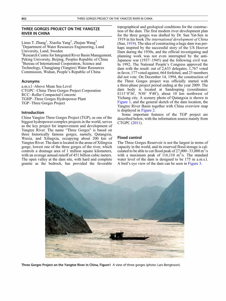
802 THREE GORGES PROJECT ON THE YANGTZE RIVER IN CHINA

THREE GORGES PROJECT ON THE YANGTZERIVER IN CHINA

Linus T. Zhang1, Xiaoliu Yang2, Zhujun Wang31Department of Water Resources Engineering, LundUniversity, Lund, Sweden2Research Centre for Integrated River BasinManagement,Peking University, Beijing, Peoples Republic of China3Bureau of International Cooperation, Science andTechnology, Changjiang (Yangtze) Water ResourcesCommission, Wuhan, People’s Republic of China

Acronymsa.m.s.l–Above Mean Sea LevelCTGPC–China Three Gorges Project CorporationRCC–Roller Compacted ConcreteTGHP–Three Gorges Hydropower PlantTGP–Three Gorges Project

IntroductionChina Yangtze Three Gorges Project (TGP), as one of thebiggest hydropower-complex projects in the world, servesas the key project for improvement and development ofYangtze River. The name “Three Gorges” is based onthree historically famous gorges, namely, Qutangxia,Wuxia, and Xilingxia, occupying about 200 km ofYangtze River. The dam is located in the areas of Xilingxiagorge, lowest one of the three gorges of the river, whichcontrols a drainage area of 1 million square kilometers,with an average annual runoff of 451 billion cubic meters.The open valley at the dam site, with hard and completegranite as the bedrock, has provided the favorable

Three Gorges Project on the Yangtze River in China, Figure1 A v

topographical and geological conditions for the construc-tion of the dam. The first modern river development planfor the three gorges was drafted by Dr. Sun Yat-Sen in1919 in his book The international development of China(Sun, 1919). The idea of constructing a huge damwas per-haps inspired by the successful story of the US HooverDam during the 1930s, and the official investigating andplanning work was not even interrupted by the anti-Japanese war (1937–1945) and the following civil war.In 1992, The National People’s Congress approved thedam with the result: out of 2,633 delegates, 1,767 votedin favor, 177 voted against, 664 forfeited, and 25 membersdid not vote. On December 14, 1994, the construction ofthe Three Gorges project was officially started witha three-phase project period ending at the year 2009. Thedam body is located at Sandouping (coordinates:E111�00360, N30� 90480), about 10 km northwest ofYichang city. A scenery photo of Qutangxia is shown inFigure 1, and the general sketch of the dam location, theYangtze River Basin together with China overview mapis displayed in Figure 2.

Some important features of the TGP project aredescribed below, with the information source mainly fromCTGPC (2011).

Flood controlThe Three Gorges Reservoir is not the largest in terms ofcapacity in the world, and its reserved flood storage is cal-culated to be able to cut flood peak of 27,000–33,000m3/swith a maximum peak of 116,110 m3/s. The standardwater level of the dam is designed to be 175 m a.m.s.l.A bird’s eye view of the dam can be seen in Figure 3.

iew of three gorges (photo: Lars Bengtsson).

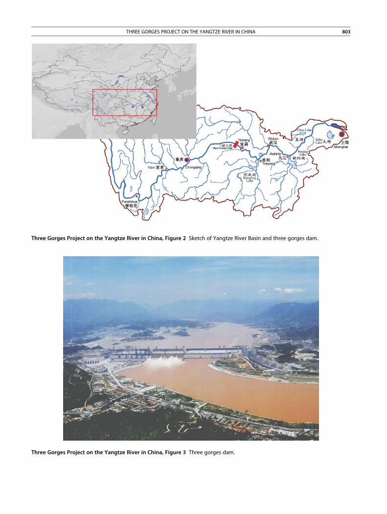
Three Gorges Project on the Yangtze River in China, Figure 3 Three gorges dam.

Three Gorges Project on the Yangtze River in China, Figure 2 Sketch of Yangtze River Basin and three gorges dam.

THREE GORGES PROJECT ON THE YANGTZE RIVER IN CHINA 803

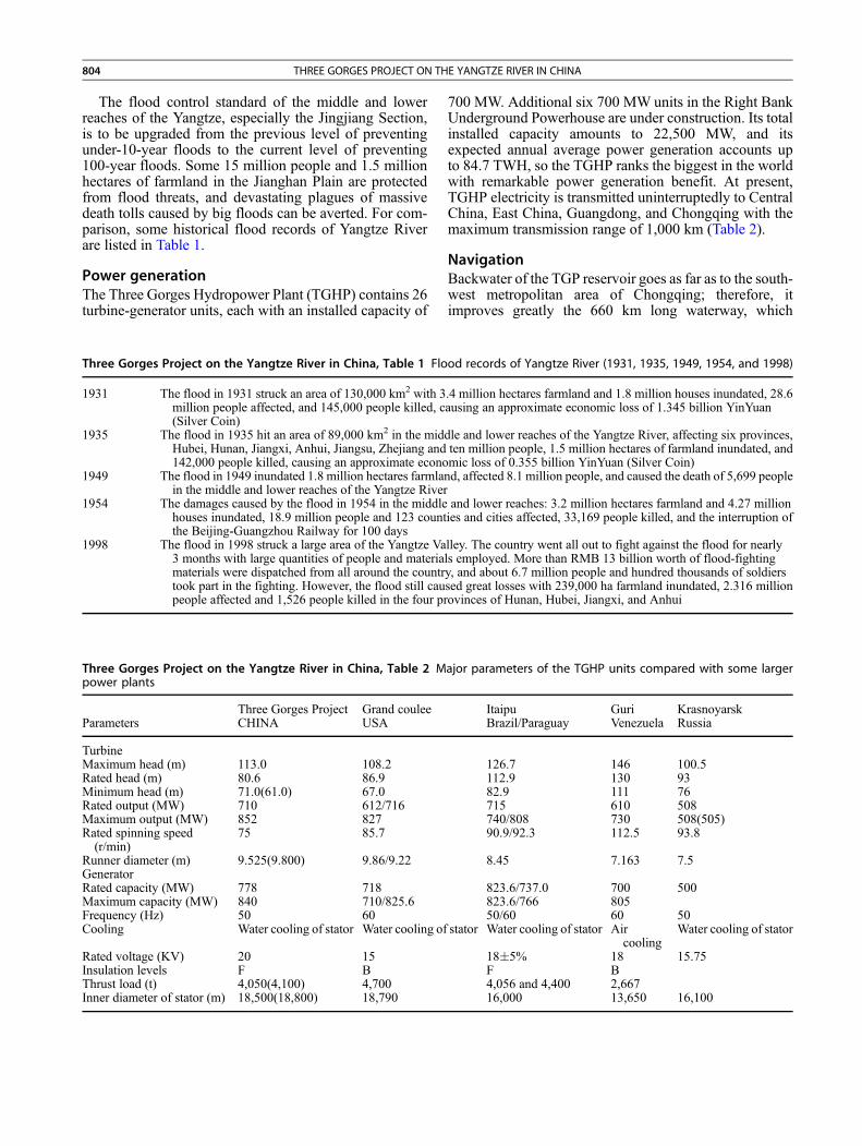
804 THREE GORGES PROJECT ON THE YANGTZE RIVER IN CHINA

The flood control standard of the middle and lowerreaches of the Yangtze, especially the Jingjiang Section,is to be upgraded from the previous level of preventingunder-10-year floods to the current level of preventing100-year floods. Some 15 million people and 1.5 millionhectares of farmland in the Jianghan Plain are protectedfrom flood threats, and devastating plagues of massivedeath tolls caused by big floods can be averted. For com-parison, some historical flood records of Yangtze Riverare listed in Table 1.

Power generationThe Three Gorges Hydropower Plant (TGHP) contains 26turbine-generator units, each with an installed capacity of

Three Gorges Project on the Yangtze River in China, Table 1 Flo

1931 The flood in 1931 struck an area of 130,000 km2 with 3million people affected, and 145,000 people killed, c(Silver Coin)

1935 The flood in 1935 hit an area of 89,000 km2 in the midHubei, Hunan, Jiangxi, Anhui, Jiangsu, Zhejiang and142,000 people killed, causing an approximate econo

1949 The flood in 1949 inundated 1.8 million hectares farmlain the middle and lower reaches of the Yangtze River

1954 The damages caused by the flood in 1954 in the middlehouses inundated, 18.9 million people and 123 countthe Beijing-Guangzhou Railway for 100 days

1998 The flood in 1998 struck a large area of the Yangtze Va3 months with large quantities of people and materiamaterials were dispatched from all around the countrtook part in the fighting. However, the flood still caupeople affected and 1,526 people killed in the four pr

Three Gorges Project on the Yangtze River in China, Table 2 Mpower plants

ParametersThree Gorges Project Grand couleeCHINA USA

TurbineMaximum head (m) 113.0 108.2Rated head (m) 80.6 86.9Minimum head (m) 71.0(61.0) 67.0Rated output (MW) 710 612/716Maximum output (MW) 852 827Rated spinning speed(r/min)

75 85.7

Runner diameter (m) 9.525(9.800) 9.86/9.22GeneratorRated capacity (MW) 778 718Maximum capacity (MW) 840 710/825.6Frequency (Hz) 50 60Cooling Water cooling of stator Water cooling of

Rated voltage (KV) 20 15Insulation levels F BThrust load (t) 4,050(4,100) 4,700Inner diameter of stator (m) 18,500(18,800) 18,790

700 MW. Additional six 700 MW units in the Right BankUnderground Powerhouse are under construction. Its totalinstalled capacity amounts to 22,500 MW, and itsexpected annual average power generation accounts upto 84.7 TWH, so the TGHP ranks the biggest in the worldwith remarkable power generation benefit. At present,TGHP electricity is transmitted uninterruptedly to CentralChina, East China, Guangdong, and Chongqing with themaximum transmission range of 1,000 km (Table 2).

NavigationBackwater of the TGP reservoir goes as far as to the south-west metropolitan area of Chongqing; therefore, itimproves greatly the 660 km long waterway, which

od records of Yangtze River (1931, 1935, 1949, 1954, and 1998)

.4 million hectares farmland and 1.8 million houses inundated, 28.6ausing an approximate economic loss of 1.345 billion YinYuan

dle and lower reaches of the Yangtze River, affecting six provinces,ten million people, 1.5 million hectares of farmland inundated, andmic loss of 0.355 billion YinYuan (Silver Coin)nd, affected 8.1 million people, and caused the death of 5,699 people

and lower reaches: 3.2 million hectares farmland and 4.27 millionies and cities affected, 33,169 people killed, and the interruption of

lley. The country went all out to fight against the flood for nearlyls employed. More than RMB 13 billion worth of flood-fightingy, and about 6.7 million people and hundred thousands of soldierssed great losses with 239,000 ha farmland inundated, 2.316 millionovinces of Hunan, Hubei, Jiangxi, and Anhui

ajor parameters of the TGHP units compared with some larger

Itaipu Guri KrasnoyarskBrazil/Paraguay Venezuela Russia

126.7 146 100.5112.9 130 9382.9 111 76715 610 508740/808 730 508(505)90.9/92.3 112.5 93.8

8.45 7.163 7.5

823.6/737.0 700 500823.6/766 80550/60 60 50

stator Water cooling of stator Aircooling

Water cooling of stator

18�5% 18 15.75F B4,056 and 4,400 2,66716,000 13,650 16,100

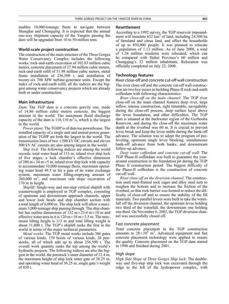
THREE GORGES PROJECT ON THE YANGTZE RIVER IN CHINA 805

enables 10,000-tonnage fleets to navigate betweenShanghai and Chongqing. It is expected that the annualone-way shipment capacity of the Yangtze passing thedam will be upgraded from 10 to 50 million tons.

World-scale project constructionThe construction of the main structure of the Three GorgesWater Conservancy Complex includes the followingworks: rock-and-earth excavation of 102.83 million cubicmeters, concrete placement of 27.94 million cubic meters,rock-and-earth refill of 31.98 million cubic meters, metalframe installation of 256,500 t, and installation oftwenty-six 700 MW turbine-generator units. Except theindex of rock-and-earth refill, all the indices are the big-gest among water conservancy projects which are alreadybuilt or under construction.

Main infrastructureDam: The TGP dam is a concrete gravity one, madeof 14.86 million cubic meters concrete, the biggestamount in the world. The maximum flood dischargecapacity of the dam is 116,110 m3/s, which is the largestin the world.

Power plant: The TGHP is of dam toe powerhouse. Theinstalled capacity of a single unit and annual power gener-ation of the TGHP are both the largest in the world. Thetransmission lines of two�500 kV DC circuits and eleven500 kVAC circuits are also among largest in the world.

Ship lock: The following indices are among the worldrecords: total water head of 113 m, inland river ship lockof five stages, a lock chamber’s effective dimensionof 280 m�34 m�5 m, inland river ship lock with capacityto accommodate 10,000-tonnage fleets, maximum operat-ing water head 49.5 m for a gate of its water exchangesystem, maximum water filling-emptying amount of260,000 m3, and maximum side slope excavation of170 m in height.

Shiplift: Single-way and one-step vertical shiplift withcounterweight is employed in TGP complex, consistingof upstream and downstream approach channels, upperand lower lock heads and ship chamber section witha total length of 6,000 m. The ship lock will allow a maxi-mum 3,000-tonnage ship passing through. The ship cham-ber has outline dimensions of 132 m�23.4 m�10 m andeffective water area in it is 120 m�18 m�3.5 m. The max-imum lifting height is 113 m and total lifting weight isabout 11,800 t. The TGP’s shiplift ranks the first in theworld in terms of the major technical parameters.

Metal works: The TGP metal works include 386 gatesof various kinds, 139 hoists of various kinds, 26 pen-stocks, all of which add up to about 256,500 t. Theoverall work quantity ranks the top among the world’shydraulic projects. The following indices are also the big-gest in the world: the penstock’s inner diameter of 12.4 m,the maximum height of ship lock miter gate of 38.25 m,and operating water head of 36.25 m, single gate’s weightof 850 t.

ResettlementAccording to a 1992 survey, the TGP reservoir impound-ment will inundate 632 km2 of land, including 24,500 haof farmland and citrus land, and affect the householdsof up to 850,000 people. It was planned to relocatea population of 1.13 million. As of June 2008, a totalof 1.24 million residents were relocated, which canbe compared with Hubei Province’s 60 million andChongqing’s 32 million inhabitants. Relocation wasofficially completed on July 22, 2008.

Technology featuresRiver close-off and concrete cut-off wall constructionThe river close-off and the concrete cut-off wall construc-tion are two key issues in building Phase-II rock-and-earthcofferdam with following characteristics:

River close-off on the main channel: The TGP riverclose-off on the main channel features deep river, largeinflow, intense construction, tight timetable, navigabilityduring the close-off process, deep surface layer abovethe levee foundation, and other difficulties. The TGPdam is situated at the backwater region of the GezhoubaReservoir, and during the close-off the maximum waterdepth at the riverbed was 60 m. It is crucial to preventlevee break and keep the levee stable during the bank-offadvance. The solution was to adopt the program of pre-leveling, upstream single levee blocking, simultaneousbank-off advance from both banks, and downstreamfollow-up advance.

Deep water cofferdam and concrete cut-off wall: TheTGP Phase-II cofferdam was built to guarantee the year-around construction in the foundation pit during the TGPPhase II construction period. The biggest difficulty ofthe Phase-II cofferdam is the construction of concretecut-off wall.

River close-off on the diversion channel: The construc-tion used steel-framed rock cages and alloy steel nets toroughen the bottom and to increase the friction of theriverbed, so that rock barrier was formed to reduce the dif-ficulty of close-off and to ensure the stability of the fillmaterials. Two parallel levees were built to take the water-fall off the diversion channel, the upstream levee holdingtwo third of the waterfall, the downstream one holdingone third. On November 6, 2002, the TGP diversion chan-nel was successfully closed off.

Fast concrete placementTotal concrete placement in the TGP constructionamounts to 28�106 m3. Advanced equipment and fastconcrete placement technology were applied to ensurethe quality. Concrete placement on the TGP dam startedin 1998 and finished during 2001.

High slopeHigh Side Slope of Three Gorges Ship lock: The double-way and five-step ship lock was excavated through theridge to the left of the hydropower complex, with

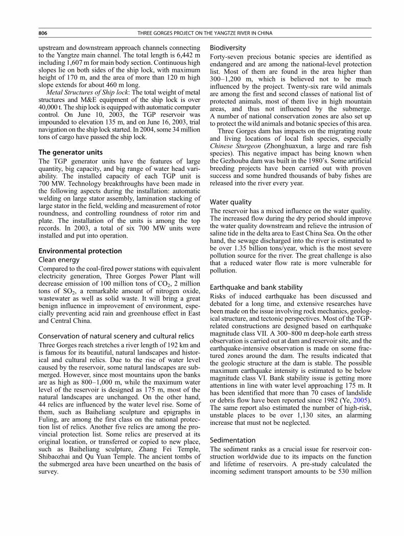
806 THREE GORGES PROJECT ON THE YANGTZE RIVER IN CHINA

upstream and downstream approach channels connectingto the Yangtze main channel. The total length is 6,442 mincluding 1,607m for main body section. Continuous highslopes lie on both sides of the ship lock, with maximumheight of 170 m, and the area of more than 120 m highslope extends for about 460 m long.

Metal Structures of Ship lock: The total weight of metalstructures and M&E equipment of the ship lock is over40,000 t. The ship lock is equippedwith automatic computercontrol. On June 10, 2003, the TGP reservoir wasimpounded to elevation 135 m, and on June 16, 2003, trialnavigation on the ship lock started. In 2004, some 34milliontons of cargo have passed the ship lock.

The generator unitsThe TGP generator units have the features of largequantity, big capacity, and big range of water head vari-ability. The installed capacity of each TGP unit is700 MW. Technology breakthroughs have been made inthe following aspects during the installation: automaticwelding on large stator assembly, lamination stacking oflarge stator in the field, welding and measurement of rotorroundness, and controlling roundness of rotor rim andplate. The installation of the units is among the toprecords. In 2003, a total of six 700 MW units wereinstalled and put into operation.

Environmental protectionClean energyCompared to the coal-fired power stations with equivalentelectricity generation, Three Gorges Power Plant willdecrease emission of 100 million tons of CO2, 2 milliontons of SO2, a remarkable amount of nitrogen oxide,wastewater as well as solid waste. It will bring a greatbenign influence in improvement of environment, espe-cially preventing acid rain and greenhouse effect in Eastand Central China.

Conservation of natural scenery and cultural relicsThree Gorges reach stretches a river length of 192 km andis famous for its beautiful, natural landscapes and histor-ical and cultural relics. Due to the rise of water levelcaused by the reservoir, some natural landscapes are sub-merged. However, since most mountains upon the banksare as high as 800–1,000 m, while the maximum waterlevel of the reservoir is designed as 175 m, most of thenatural landscapes are unchanged. On the other hand,44 relics are influenced by the water level rise. Some ofthem, such as Baiheliang sculpture and epigraphs inFuling, are among the first class on the national protec-tion list of relics. Another five relics are among the pro-vincial protection list. Some relics are preserved at itsoriginal location, or transferred or copied to new place,such as Baiheliang sculpture, Zhang Fei Temple,Shibaozhai and Qu Yuan Temple. The ancient tombs ofthe submerged area have been unearthed on the basis ofsurvey.

BiodiversityForty-seven precious botanic species are identified asendangered and are among the national-level protectionlist. Most of them are found in the area higher than300–1,200 m, which is believed not to be muchinfluenced by the project. Twenty-six rare wild animalsare among the first and second classes of national list ofprotected animals, most of them live in high mountainareas, and thus not influenced by the submerge.A number of national conservation zones are also set upto protect the wild animals and botanic species of this area.

Three Gorges dam has impacts on the migrating routeand living locations of local fish species, especiallyChinese Sturgeon (Zhonghuaxun, a large and rare fishspecies). This negative impact has being known whenthe Gezhouba dam was built in the 1980’s. Some artificialbreeding projects have been carried out with provensuccess and some hundred thousands of baby fishes arereleased into the river every year.

Water qualityThe reservoir has a mixed influence on the water quality.The increased flow during the dry period should improvethe water quality downstream and relieve the intrusion ofsaline tide in the delta area to East China Sea. On the otherhand, the sewage discharged into the river is estimated tobe over 1.35 billion tons/year, which is the most severepollution source for the river. The great challenge is alsothat a reduced water flow rate is more vulnerable forpollution.

Earthquake and bank stabilityRisks of induced earthquake has been discussed anddebated for a long time, and extensive researches havebeen made on the issue involving rock mechanics, geolog-ical structure, and tectonic perspectives. Most of the TGP-related constructions are designed based on earthquakemagnitude class VII. A 300~800 m deep-hole earth stressobservation is carried out at dam and reservoir site, and theearthquake-intensive observation is made on some frac-tured zones around the dam. The results indicated thatthe geologic structure at the dam is stable. The possiblemaximum earthquake intensity is estimated to be belowmagnitude class VI. Bank stability issue is getting moreattentions in line with water level approaching 175 m. Ithas been identified that more than 70 cases of landslideor debris flow have been reported since 1982 (Ye, 2005).The same report also estimated the number of high-risk,unstable places to be over 1,130 sites, an alarmingincrease that must not be neglected.

SedimentationThe sediment ranks as a crucial issue for reservoir con-struction worldwide due to its impacts on the functionand lifetime of reservoirs. A pre-study calculated theincoming sediment transport amounts to be 530 million

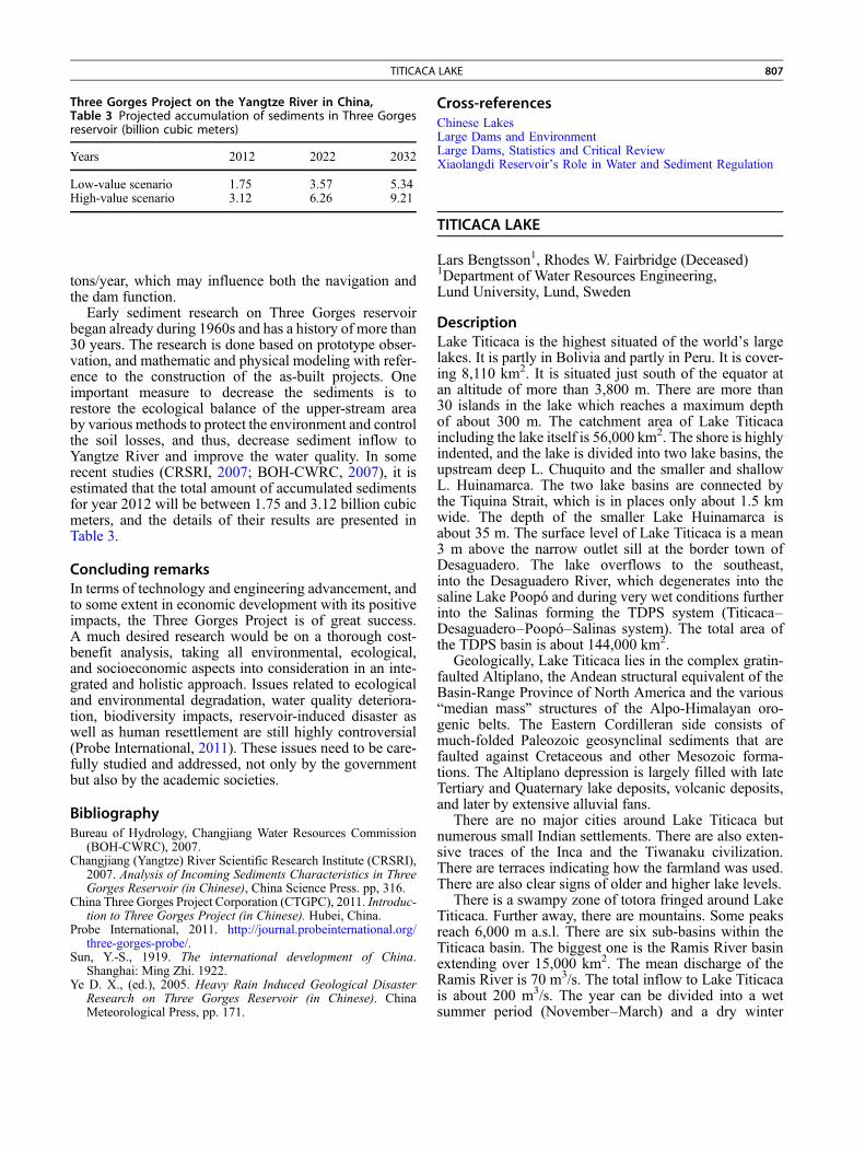
Three Gorges Project on the Yangtze River in China,Table 3 Projected accumulation of sediments in Three Gorgesreservoir (billion cubic meters)

Years 2012 2022 2032

Low-value scenario 1.75 3.57 5.34High-value scenario 3.12 6.26 9.21

TITICACA LAKE 807

tons/year, which may influence both the navigation andthe dam function.

Early sediment research on Three Gorges reservoirbegan already during 1960s and has a history of more than30 years. The research is done based on prototype obser-vation, and mathematic and physical modeling with refer-ence to the construction of the as-built projects. Oneimportant measure to decrease the sediments is torestore the ecological balance of the upper-stream areaby various methods to protect the environment and controlthe soil losses, and thus, decrease sediment inflow toYangtze River and improve the water quality. In somerecent studies (CRSRI, 2007; BOH-CWRC, 2007), it isestimated that the total amount of accumulated sedimentsfor year 2012 will be between 1.75 and 3.12 billion cubicmeters, and the details of their results are presented inTable 3.

Concluding remarksIn terms of technology and engineering advancement, andto some extent in economic development with its positiveimpacts, the Three Gorges Project is of great success.A much desired research would be on a thorough cost-benefit analysis, taking all environmental, ecological,and socioeconomic aspects into consideration in an inte-grated and holistic approach. Issues related to ecologicaland environmental degradation, water quality deteriora-tion, biodiversity impacts, reservoir-induced disaster aswell as human resettlement are still highly controversial(Probe International, 2011). These issues need to be care-fully studied and addressed, not only by the governmentbut also by the academic societies.

BibliographyBureau of Hydrology, Changjiang Water Resources Commission

(BOH-CWRC), 2007.Changjiang (Yangtze) River Scientific Research Institute (CRSRI),

2007. Analysis of Incoming Sediments Characteristics in ThreeGorges Reservoir (in Chinese), China Science Press. pp, 316.

China Three Gorges Project Corporation (CTGPC), 2011. Introduc-tion to Three Gorges Project (in Chinese). Hubei, China.

Probe International, 2011. http://journal.probeinternational.org/three-gorges-probe/.

Sun, Y.-S., 1919. The international development of China.Shanghai: Ming Zhi. 1922.

Ye D. X., (ed.), 2005. Heavy Rain Induced Geological DisasterResearch on Three Gorges Reservoir (in Chinese). ChinaMeteorological Press, pp. 171.

Cross-referencesChinese LakesLarge Dams and EnvironmentLarge Dams, Statistics and Critical ReviewXiaolangdi Reservoir’s Role in Water and Sediment Regulation

TITICACA LAKE

Lars Bengtsson1, Rhodes W. Fairbridge (Deceased)1Department of Water Resources Engineering,Lund University, Lund, Sweden

DescriptionLake Titicaca is the highest situated of the world’s largelakes. It is partly in Bolivia and partly in Peru. It is cover-ing 8,110 km2. It is situated just south of the equator atan altitude of more than 3,800 m. There are more than30 islands in the lake which reaches a maximum depthof about 300 m. The catchment area of Lake Titicacaincluding the lake itself is 56,000 km2. The shore is highlyindented, and the lake is divided into two lake basins, theupstream deep L. Chuquito and the smaller and shallowL. Huinamarca. The two lake basins are connected bythe Tiquina Strait, which is in places only about 1.5 kmwide. The depth of the smaller Lake Huinamarca isabout 35 m. The surface level of Lake Titicaca is a mean3 m above the narrow outlet sill at the border town ofDesaguadero. The lake overflows to the southeast,into the Desaguadero River, which degenerates into thesaline Lake Poopó and during very wet conditions furtherinto the Salinas forming the TDPS system (Titicaca–Desaguadero–Poopó–Salinas system). The total area ofthe TDPS basin is about 144,000 km2.

Geologically, Lake Titicaca lies in the complex gratin-faulted Altiplano, the Andean structural equivalent of theBasin-Range Province of North America and the various“median mass” structures of the Alpo-Himalayan oro-genic belts. The Eastern Cordilleran side consists ofmuch-folded Paleozoic geosynclinal sediments that arefaulted against Cretaceous and other Mesozoic forma-tions. The Altiplano depression is largely filled with lateTertiary and Quaternary lake deposits, volcanic deposits,and later by extensive alluvial fans.

There are no major cities around Lake Titicaca butnumerous small Indian settlements. There are also exten-sive traces of the Inca and the Tiwanaku civilization.There are terraces indicating how the farmland was used.There are also clear signs of older and higher lake levels.

There is a swampy zone of totora fringed around LakeTiticaca. Further away, there are mountains. Some peaksreach 6,000 m a.s.l. There are six sub-basins within theTiticaca basin. The biggest one is the Ramis River basinextending over 15,000 km2. The mean discharge of theRamis River is 70 m3/s. The total inflow to Lake Titicacais about 200 m3/s. The year can be divided into a wetsummer period (November–March) and a dry winter

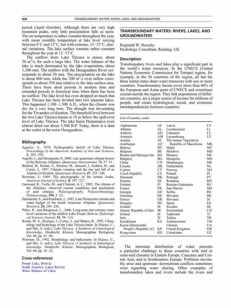
808 TRANSBOUNDARY WATERS: RIVERS, LAKES, AND GROUNDWATERS

period (April–October). Although there are very highmountain peaks, only little precipitation falls as snow.The air temperature is rather constant throughout the year,with mean monthly temperature at lake level varyingbetween 6�C and 12�C, but with extreme, 15–25�C, diur-nal variations. The lake surface remains rather constantthroughout the year at 12–13�C.

The outflow from Lake Titicaca is minor, about30 m3/s, for such a large lake. The water balance of thelake is much dominated by the lake evaporation, about1,300 mm. The outflow with the Desaguadero River cor-responds to about 50 mm. The precipitation on the lakeis about 800 mm, while the 200 m3/s river inflow corre-sponds to about 550 mm relative to the lake surface area.There have been short periods in modern time andextended periods in historical time when there has beenno outflow. The lake level has even dropped so much thatLake Titicaca has been divided into two separate lakes.This happened 1,100–1,500 A.D., when the climate wasdry for a very long time. The drought was devastatingfor the Tiwanaku civilization. The threshold level betweenthe two Lake Titicaca basins is 19 m below the spill-overlevel of Lake Titicaca. The lake basin Huinamarca evenalmost dried out about 3,500 B.P. Today, there is a damat the outlet at the town Desaguadero.

BibliographyAgassiz, A., 1876. Hydrographic sketch of Lake Titicaca.

Proceedings of the American Academy of Arts and Sciences,2, 283–292.

Argollo, J., and Mourguiart, P., 2000. Late quaternary climate historyof the Bolivian Altiplano. Quaternary International, 72, 37–51.

Binford, M., Kolata, A., Brenner, M., Janusek, J., Seddon, M., andCurtis, J., 1997. Climate variation and the rise and fall of anAndean civilization. Quaternary Research, 47, 235–248.

Bowman, I., 1909. The physiography of the central Andes.American Journal of Science, 8, 197–217.

Garreaud, R., Vuille, M., and Clement, A. C., 2003. The climate ofthe Altiplano: observed current conditions and mechanismof past changes. Palaeogeography, Palaeoclimatology,Palaeoecology, 194, 5–22.

Hastenrath, S., and Kutzbach, J., 1985. Late Pleistocene climate andwater budget of the South American Altiplano. QuaternaryResearch, 24, 249–256.

Pillco, R., and Bengtsson, L., 2006. Long-term and extreme waterlevel variations of the shallow Lake Poopó, Bolivia. Hydrologi-cal Sciences Journal, 51, 98–114.

Roche, M. A., Bourges, J., Cortez, J., and Mattos, R., 1992. Clima-tology and hydrology of the Lake Titicaca basin. In Dejoux, C.,and Iltis, A. (eds.), Lake Titicaca. A Synthesis of LimnologicalKnowledge. Dordrecht: Kluwer. Monographiae Biologicae,Vol. 68, pp. 63–88.

Wirrman, D., 1992. Morphology and bathymetry. In Dejoux, C.,and Iltis, A. (eds.), Lake Titicaca. A Synthesis of limnologicalknowledge. Dordrecht: Kluwer. Monographiae Biologicae,Vol. 68, pp. 16–22.

Cross-referencesPoopó Lake, BoliviaSouth America, Lakes ReviewWater Balance of Lakes

TRANSBOUNDARY WATERS: RIVERS, LAKES, ANDGROUNDWATERS

Reginald W. HerschyHydrology Consultant, Reading, UK

DescriptionTransboundary rivers and lakes play a significant part inthe world’s water resources. In the UNECE (UnitedNations Economic Commission for Europe) region, forexample, in the 56 countries of the region, all but thethree island states share water resources with one or morecountries. Transboundary basins cover more than 40% ofthe European and Asian parts of UNECE and sometimesextend outside the region. They link populations of differ-ent countries, are a major source of income for millions ofpeople, and create hydrological, social, and economicinterdependencies between countries.

List of country codes

Afghanistan

AF Latvia LV Albania AL Liechtenstein LI Andorra AD Lithuania LT Armenia AM Luxembourg LU Austria AT The former Yugoslavia Azerbaijan AZ Republic of Macedonia MK Belarus BY Malta MT Belgium BE Moldova MD Bosnia and Herzegovina BA Monaco MC Bulgaria BG Mongolia MN China CN Montenegro ME Croatia HR Netherlands NL Cyprus CY Norway NO Czech Republic CZ Poland PL Denmark DK Portugal PT Estonia EE Romania RO Finland FI Russian Federation RU France FR San Marino SM Georgia GE Serbia RS Germany DE Slovakia SK Greece GR Slovenia SI Hungary HU Spain ES Iceland IS Sweden SE Islamic Republic of Iran IR Switzerland CH Ireland IE Tajikistan TJ Italy IT Turkey TR Kazakhstan KZ Turkmenistan TM Korea (Democratic Ukraine UA People’s Republic of ) KP United Kingdom GB

Kyrgyzstan

KG Uzbekistan UZ

The interstate distribution of water presentsa particular challenge to those countries with arid orsemi-arid climates in Eastern Europe, Caucasus and Cen-tral Asia, and in Southeastern Europe. Problems inevita-bly arise and upstream–downstream conflicts sometimesexist regarding water sharing. Other examples oftransboundary lakes and rivers include the rivers and

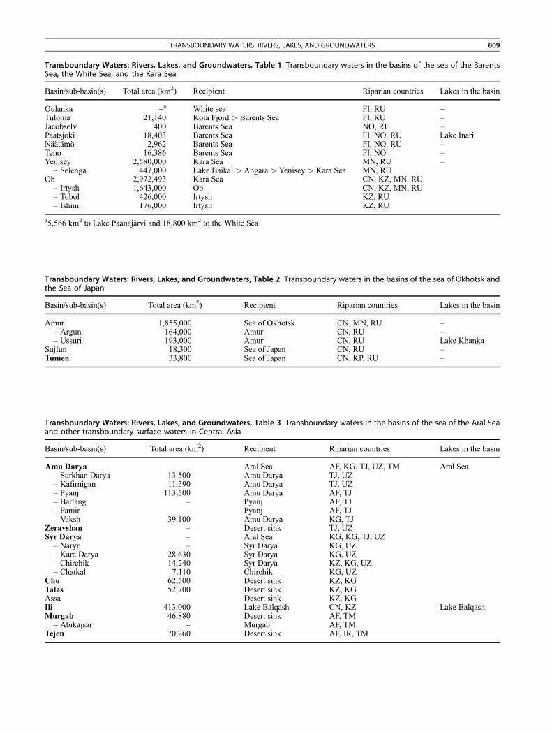
Transboundary Waters: Rivers, Lakes, and Groundwaters, Table 1 Transboundary waters in the basins of the sea of the BarentsSea, the White Sea, and the Kara Sea

Basin/sub-basin(s) Total area (km2) Recipient Riparian countries Lakes in the basin

Oulanka –a White sea FI, RU –Tuloma 21,140 Kola Fjord > Barents Sea FI, RU –Jacobselv 400 Barents Sea NO, RU –Paatsjoki 18,403 Barents Sea FI, NO, RU Lake InariNäätämö 2,962 Barents Sea FI, NO, RU –Teno 16,386 Barents Sea FI, NO –Yenisey 2,580,000 Kara Sea MN, RU –– Selenga 447,000 Lake Baikal > Angara > Yenisey > Kara Sea MN, RU

Ob 2,972,493 Kara Sea CN, KZ, MN, RU– Irtysh 1,643,000 Ob CN, KZ, MN, RU– Tobol 426,000 Irtysh KZ, RU– Ishim 176,000 Irtysh KZ, RU

a5,566 km2 to Lake Paanajärvi and 18,800 km2 to the White Sea

Transboundary Waters: Rivers, Lakes, and Groundwaters, Table 2 Transboundary waters in the basins of the sea of Okhotsk andthe Sea of Japan

Basin/sub-basin(s) Total area (km2) Recipient Riparian countries Lakes in the basin

Amur 1,855,000 Sea of Okhotsk CN, MN, RU –– Argun 164,000 Amur CN, RU –– Ussuri 193,000 Amur CN, RU Lake Khanka

Sujfun 18,300 Sea of Japan CN, RU –Tumen 33,800 Sea of Japan CN, KP, RU –

Transboundary Waters: Rivers, Lakes, and Groundwaters, Table 3 Transboundary waters in the basins of the sea of the Aral Seaand other transboundary surface waters in Central Asia

Basin/sub-basin(s) Total area (km2) Recipient Riparian countries Lakes in the basin

Amu Darya – Aral Sea AF, KG, TJ, UZ, TM Aral Sea– Surkhan Darya 13,500 Amu Darya TJ, UZ– Kafirnigan 11,590 Amu Darya TJ, UZ– Pyanj 113,500 Amu Darya AF, TJ– Bartang – Pyanj AF, TJ– Pamir – Pyanj AF, TJ– Vaksh 39,100 Amu Darya KG, TJ

Zeravshan – Desert sink TJ, UZSyr Darya – Aral Sea KG, KG, TJ, UZ– Naryn – Syr Darya KG, UZ– Kara Darya 28,630 Syr Darya KG, UZ– Chirchik 14,240 Syr Darya KZ, KG, UZ– Chatkal 7,110 Chirchik KG, UZ

Chu 62,500 Desert sink KZ, KGTalas 52,700 Desert sink KZ, KGAssa – Desert sink KZ, KGIli 413,000 Lake Balqash CN, KZ Lake BalqashMurgab 46,880 Desert sink AF, TM– Abikajsar – Murgab AF, TM

Tejen 70,260 Desert sink AF, IR, TM

TRANSBOUNDARY WATERS: RIVERS, LAKES, AND GROUNDWATERS 809

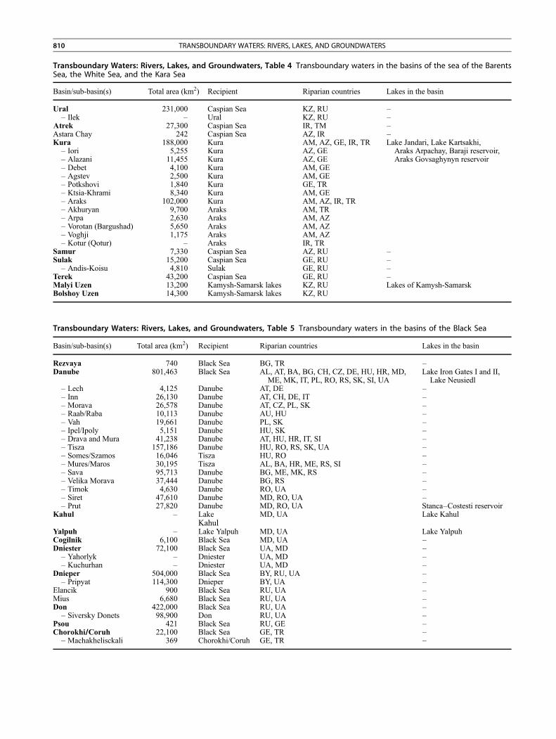
Transboundary Waters: Rivers, Lakes, and Groundwaters, Table 4 Transboundary waters in the basins of the sea of the BarentsSea, the White Sea, and the Kara Sea

Basin/sub-basin(s) Total area (km2) Recipient Riparian countries Lakes in the basin

Ural 231,000 Caspian Sea KZ, RU –– Ilek – Ural KZ, RU –

Atrek 27,300 Caspian Sea IR, TM –Astara Chay 242 Caspian Sea AZ, IR –Kura 188,000 Kura AM, AZ, GE, IR, TR Lake Jandari, Lake Kartsakhi,

Araks Arpachay, Baraji reservoir,Araks Govsaghynyn reservoir

– Iori 5,255 Kura AZ, GE– Alazani 11,455 Kura AZ, GE– Debet 4,100 Kura AM, GE– Agstev 2,500 Kura AM, GE– Potkshovi 1,840 Kura GE, TR– Ktsia-Khrami 8,340 Kura AM, GE– Araks 102,000 Kura AM, AZ, IR, TR– Akhuryan 9,700 Araks AM, TR– Arpa 2,630 Araks AM, AZ– Vorotan (Bargushad) 5,650 Araks AM, AZ– Voghji 1,175 Araks AM, AZ– Kotur (Qotur) – Araks IR, TR

Samur 7,330 Caspian Sea AZ, RU –Sulak 15,200 Caspian Sea GE, RU –– Andis-Koisu 4,810 Sulak GE, RU –

Terek 43,200 Caspian Sea GE, RU –Malyi Uzen 13,200 Kamysh-Samarsk lakes KZ, RU Lakes of Kamysh-SamarskBolshoy Uzen 14,300 Kamysh-Samarsk lakes KZ, RU

Transboundary Waters: Rivers, Lakes, and Groundwaters, Table 5 Transboundary waters in the basins of the Black Sea

Basin/sub-basin(s) Total area (km2) Recipient Riparian countries Lakes in the basin

Rezvaya 740 Black Sea BG, TR –Danube 801,463 Black Sea AL, AT, BA, BG, CH, CZ, DE, HU, HR, MD,

ME, MK, IT, PL, RO, RS, SK, SI, UALake Iron Gates I and II,Lake Neusiedl

– Lech 4,125 Danube AT, DE –– Inn 26,130 Danube AT, CH, DE, IT –– Morava 26,578 Danube AT, CZ, PL, SK –– Raab/Raba 10,113 Danube AU, HU –– Vah 19,661 Danube PL, SK –– Ipel/Ipoly 5,151 Danube HU, SK –– Drava and Mura 41,238 Danube AT, HU, HR, IT, SI –– Tisza 157,186 Danube HU, RO, RS, SK, UA –– Somes/Szamos 16,046 Tisza HU, RO –– Mures/Maros 30,195 Tisza AL, BA, HR, ME, RS, SI –– Sava 95,713 Danube BG, ME, MK, RS –– Velika Morava 37,444 Danube BG, RS –– Timok 4,630 Danube RO, UA –– Siret 47,610 Danube MD, RO, UA –– Prut 27,820 Danube MD, RO, UA Stanca–Costesti reservoir

Kahul – LakeKahul

MD, UA Lake Kahul

Yalpuh – Lake Yalpuh MD, UA Lake YalpuhCogilnik 6,100 Black Sea MD, UA –Dniester 72,100 Black Sea UA, MD –– Yahorlyk – Dniester UA, MD –– Kuchurhan – Dniester UA, MD –

Dnieper 504,000 Black Sea BY, RU, UA –– Pripyat 114,300 Dnieper BY, UA –

Elancik 900 Black Sea RU, UA –Mius 6,680 Black Sea RU, UA –Don 422,000 Black Sea RU, UA –– Siversky Donets 98,900 Don RU, UA –

Psou 421 Black Sea RU, GE –Chorokhi/Coruh 22,100 Black Sea GE, TR –– Machakhelisckali 369 Chorokhi/Coruh GE, TR –

810 TRANSBOUNDARY WATERS: RIVERS, LAKES, AND GROUNDWATERS

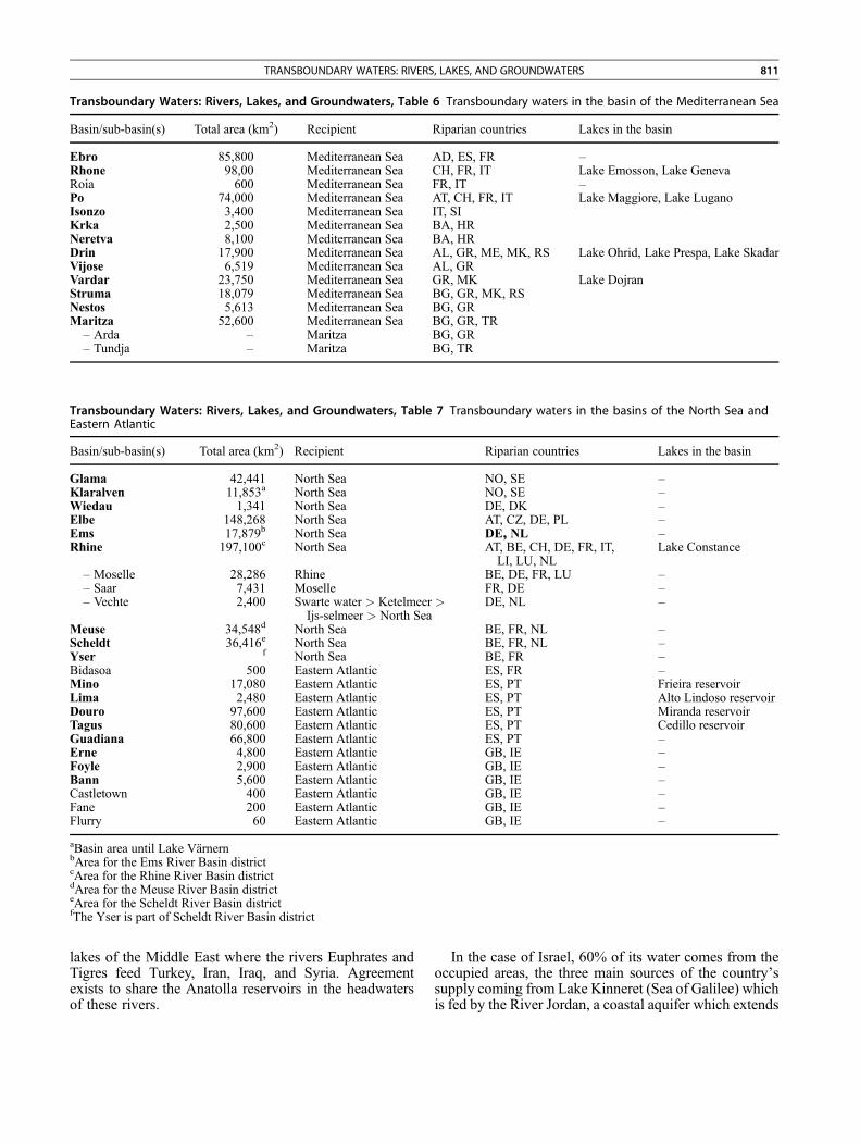
Transboundary Waters: Rivers, Lakes, and Groundwaters, Table 6 Transboundary waters in the basin of the Mediterranean Sea

Basin/sub-basin(s) Total area (km2) Recipient Riparian countries Lakes in the basin

Ebro 85,800 Mediterranean Sea AD, ES, FR –Rhone 98,00 Mediterranean Sea CH, FR, IT Lake Emosson, Lake GenevaRoia 600 Mediterranean Sea FR, IT –Po 74,000 Mediterranean Sea AT, CH, FR, IT Lake Maggiore, Lake LuganoIsonzo 3,400 Mediterranean Sea IT, SIKrka 2,500 Mediterranean Sea BA, HRNeretva 8,100 Mediterranean Sea BA, HRDrin 17,900 Mediterranean Sea AL, GR, ME, MK, RS Lake Ohrid, Lake Prespa, Lake SkadarVijose 6,519 Mediterranean Sea AL, GRVardar 23,750 Mediterranean Sea GR, MK Lake DojranStruma 18,079 Mediterranean Sea BG, GR, MK, RSNestos 5,613 Mediterranean Sea BG, GRMaritza 52,600 Mediterranean Sea BG, GR, TR– Arda – Maritza BG, GR– Tundja – Maritza BG, TR

Transboundary Waters: Rivers, Lakes, and Groundwaters, Table 7 Transboundary waters in the basins of the North Sea andEastern Atlantic

Basin/sub-basin(s) Total area (km2) Recipient Riparian countries Lakes in the basin

Glama 42,441 North Sea NO, SE –Klaralven 11,853a North Sea NO, SE –Wiedau 1,341 North Sea DE, DK –Elbe 148,268 North Sea AT, CZ, DE, PL –Ems 17,879b North Sea DE, NL –Rhine 197,100c North Sea AT, BE, CH, DE, FR, IT,

LI, LU, NLLake Constance

– Moselle 28,286 Rhine BE, DE, FR, LU –– Saar 7,431 Moselle FR, DE –– Vechte 2,400 Swarte water > Ketelmeer >

Ijs-selmeer > North SeaDE, NL –

Meuse 34,548d North Sea BE, FR, NL –Scheldt 36,416e North Sea BE, FR, NL –Yser f North Sea BE, FR –Bidasoa 500 Eastern Atlantic ES, FR –Mino 17,080 Eastern Atlantic ES, PT Frieira reservoirLima 2,480 Eastern Atlantic ES, PT Alto Lindoso reservoirDouro 97,600 Eastern Atlantic ES, PT Miranda reservoirTagus 80,600 Eastern Atlantic ES, PT Cedillo reservoirGuadiana 66,800 Eastern Atlantic ES, PT –Erne 4,800 Eastern Atlantic GB, IE –Foyle 2,900 Eastern Atlantic GB, IE –Bann 5,600 Eastern Atlantic GB, IE –Castletown 400 Eastern Atlantic GB, IE –Fane 200 Eastern Atlantic GB, IE –Flurry 60 Eastern Atlantic GB, IE –

aBasin area until Lake VärnernbArea for the Ems River Basin districtcArea for the Rhine River Basin districtdArea for the Meuse River Basin districteArea for the Scheldt River Basin districtfThe Yser is part of Scheldt River Basin district

TRANSBOUNDARY WATERS: RIVERS, LAKES, AND GROUNDWATERS 811

lakes of the Middle East where the rivers Euphrates andTigres feed Turkey, Iran, Iraq, and Syria. Agreementexists to share the Anatolla reservoirs in the headwatersof these rivers.

In the case of Israel, 60% of its water comes from theoccupied areas, the three main sources of the country’ssupply coming from Lake Kinneret (Sea of Galilee) whichis fed by the River Jordan, a coastal aquifer which extends

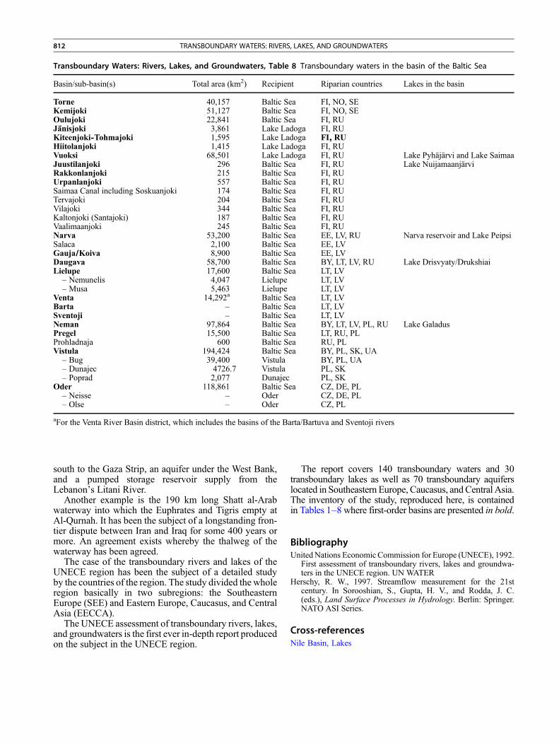
Transboundary Waters: Rivers, Lakes, and Groundwaters, Table 8 Transboundary waters in the basin of the Baltic Sea

Basin/sub-basin(s) Total area (km2) Recipient Riparian countries Lakes in the basin

Torne 40,157 Baltic Sea FI, NO, SEKemijoki 51,127 Baltic Sea FI, NO, SEOulujoki 22,841 Baltic Sea FI, RUJänisjoki 3,861 Lake Ladoga FI, RUKiteenjoki-Tohmajoki 1,595 Lake Ladoga FI, RUHiitolanjoki 1,415 Lake Ladoga FI, RUVuoksi 68,501 Lake Ladoga FI, RU Lake Pyhäjärvi and Lake SaimaaJuustilanjoki 296 Baltic Sea FI, RU Lake NuijamaanjärviRakkonlanjoki 215 Baltic Sea FI, RUUrpanlanjoki 557 Baltic Sea FI, RUSaimaa Canal including Soskuanjoki 174 Baltic Sea FI, RUTervajoki 204 Baltic Sea FI, RUVilajoki 344 Baltic Sea FI, RUKaltonjoki (Santajoki) 187 Baltic Sea FI, RUVaalimaanjoki 245 Baltic Sea FI, RUNarva 53,200 Baltic Sea EE, LV, RU Narva reservoir and Lake PeipsiSalaca 2,100 Baltic Sea EE, LVGauja/Koiva 8,900 Baltic Sea EE, LVDaugava 58,700 Baltic Sea BY, LT, LV, RU Lake Drisvyaty/DrukshiaiLielupe 17,600 Baltic Sea LT, LV– Nemunelis 4,047 Lielupe LT, LV– Musa 5,463 Lielupe LT, LV

Venta 14,292a Baltic Sea LT, LVBarta – Baltic Sea LT, LVSventoji – Baltic Sea LT, LVNeman 97,864 Baltic Sea BY, LT, LV, PL, RU Lake GaladusPregel 15,500 Baltic Sea LT, RU, PLProhladnaja 600 Baltic Sea RU, PLVistula 194,424 Baltic Sea BY, PL, SK, UA– Bug 39,400 Vistula BY, PL, UA– Dunajec 4726.7 Vistula PL, SK– Poprad 2,077 Dunajec PL, SK

Oder 118,861 Baltic Sea CZ, DE, PL– Neisse – Oder CZ, DE, PL– Olse – Oder CZ, PL

aFor the Venta River Basin district, which includes the basins of the Barta/Bartuva and Sventoji rivers

812 TRANSBOUNDARY WATERS: RIVERS, LAKES, AND GROUNDWATERS

south to the Gaza Strip, an aquifer under the West Bank,and a pumped storage reservoir supply from theLebanon’s Litani River.

Another example is the 190 km long Shatt al-Arabwaterway into which the Euphrates and Tigris empty atAl-Qurnah. It has been the subject of a longstanding fron-tier dispute between Iran and Iraq for some 400 years ormore. An agreement exists whereby the thalweg of thewaterway has been agreed.

The case of the transboundary rivers and lakes of theUNECE region has been the subject of a detailed studyby the countries of the region. The study divided the wholeregion basically in two subregions: the SoutheasternEurope (SEE) and Eastern Europe, Caucasus, and CentralAsia (EECCA).

The UNECE assessment of transboundary rivers, lakes,and groundwaters is the first ever in-depth report producedon the subject in the UNECE region.

The report covers 140 transboundary waters and 30transboundary lakes as well as 70 transboundary aquiferslocated in Southeastern Europe, Caucasus, and Central Asia.The inventory of the study, reproduced here, is containedin Tables 1–8 where first-order basins are presented in bold.

BibliographyUnited Nations Economic Commission for Europe (UNECE), 1992.

First assessment of transboundary rivers, lakes and groundwa-ters in the UNECE region. UN WATER

Herschy, R. W., 1997. Streamflow measurement for the 21stcentury. In Sorooshian, S., Gupta, H. V., and Rodda, J. C.(eds.), Land Surface Processes in Hydrology. Berlin: Springer.NATO ASI Series.

Cross-referencesNile Basin, Lakes

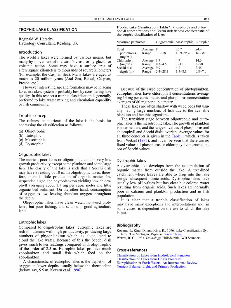
Trophic Lake Classification, Table 1 Phosphorus and chlor-ophyll concentrations and Secchi disk depths characteristic ofthe trophic classification of lakes

Measured parameter Oligotrophic Mesotrophic Eutrophic

Totalphosphorus(mg/m3)

Average 8 26.7 84.4Range 30.–18 10.9–95.6 16–386

Chlorophyll(mg/m3)

Average 1.7 4.7 14.3Range 0.3–4.5 3–11 3–78

Secchi diskdepth (m)

Average 9.9 4.2 2.45Range 5.4–28.3 1.5–8.1 0.8–7.0

TROPHIC LAKE CLASSIFICATION 813

TROPHIC LAKE CLASSIFICATION

Reginald W. HerschyHydrology Consultant, Reading, UK

IntroductionThe world’s lakes were formed by various means, butmany by movement of the earth’s crust, or by glacial orvolcanic action. Some may have a surface area ofa few square kilometers to thousands of square kilometers(for example, the Caspian Sea). Many lakes are aged asmuch as 20 million years (Aral Sea, Baikal, Caspian,Prespa, etc.).

However interesting age and formation may be, placinglakes in a class system is probably best by considering lakequality. In this respect a trophic classification is generallypreferred to lake water mixing and circulation capabilityor fish community.

Trophic conceptThe richness in nutrients of the lake is the basis foraddressing the classification as follows:

(a) Oligotrophic(b) Eutrophic(c) Mesotrophic(d) Dystrophic

Oligotrophic lakesThe nutrient-poor lakes or oligotrophic contain very lowgrowth productivity except some plankton and some largefish. The clarity of the lake is such that a Secchi diskmay have a reading of 10 m. In oligotrophic lakes, there-fore, there is little production of organic matter fewsuspended algae, the phytoplankton yielding low chloro-phyll averaging about 1.7 mg per cubic meter and littleorganic bed sediment. On the other hand, consumptionof oxygen is low, leaving abundant oxygen throughoutthe depth.

Oligotrophic lakes have clean water, no weed prob-lems, but poor fishing, and seldom in good agricultureland.

Eutrophic lakesCompared to oligotrophic lakes, eutrophic lakes arerich in nutrients with high productivity, producing largenumbers of phytoplankton which, as algae, tend tocloud the lake water. Because of this the Secchi diskgives much lower readings compared with oligotrophicof the order of 2.5 m. Eutrophic lakes produce muchzooplankton and small fish which feed on thezooplankton.

A characteristic of eutrophic lakes is the depletion ofoxygen in lower depths usually below the thermocline(below, say, 5.5 m, Kevern et al. 1996).

Because of the large concentration of phytoplankton,eutrophic lakes have chlorophyll concentrations averag-ing 14 mg per cubic meters and phosphorus concentrationaverages of 80 mg per cubic meter.

These lakes are often shallow with weed beds but usu-ally having large numbers of fish due to the availableplankton and benthic organisms.

The transition stage between oligotrophic and eutro-phic lakes is the mesotrophic lake. The growth of planktonis intermediate, and the range of values of phosphorus andchlorophyll and Secchi disks overlap. Average values forall three concepts is given in the Table 1 which is takenfrom Wetzel (1983), and it can be seen that there are nofixed values of phosphorus or chlorophyll concentrationsnor of Secchi values.

Dystrophic lakesA dystrophic lake develops from the accumulation oforganic matter from outside the lake. A tree-linedcatchment where leaves are able to drop into the lakebrings subsequent humic acids. Dystrophic lakes haveusually low pH values but has clear but colored waterresulting from organic acids. Such lakes are normallypoor in calcium and plankton production and in fishpopulation.

It is clear that a trophic classification of lakesmay have many exceptions and interpretations and, insome cases, is dependent on the use to which the lakeis put.

BibliographyKevern, N., King, D., and King, R., 1996. Lake Classification Sys-

tems. The Michigan: Riparian. www.mlswaWetzel, R. G., 1983. Limnology. Philadelphia: WB Saunders.

Cross-referencesClassification of Lakes from Hydrological FunctionClassification of Lakes from Origin ProcessesEutrophication in Fresh Waters: An International ReviewNutrient Balance, Light, and Primary Production

814 TSUNAMI EFFECT ON A COASTAL LAKE IN INDIA

TSUNAMI EFFECT ON A COASTAL LAKE IN INDIA

Kamala Kanta Satpathy1, Ajit KumarMohanty1, SudeeptaBiswas2, M. Selvanayagam2, Santosh Kumar Sarkar31Environmental & Safety Division, Indira Gandhi Centerfor Atomic Research (IGCAR), Kalpakkam, TN, India2Loyola Institute of Frontier Energy, Loyola College,Chennai, TN, India3Department of Marine Science, Calcutta University,Kolkata, India

IntroductionKalpakkam (12�340N Lat. and 80�110E Long.), situatedon the east coast of India about 80 km south ofChennai (Figure 1), is known for existence of nuclearfacilities, such as Madras Atomic Power Station(MAPS) and Prototype Fast Breeder Reactor (PFBR).The entire site covers approximately 1,500 ha. It isbestowed with a number of natural water bodies in theform of backwaters and lakes. One of them is a tinybrackish water lake (Kokilamedu lake) situated on theisolated northeastern side of the campus. It covers anarea of 0.75 sq km during monsoon period, and thespread shrinks to 0.5 sq km during summer. The averagedepth is about 1 m and has a maximum depth of 3 m.The lake provides a conducive environment for thewaders as well as for other aquatic and terrestrial faunathat inhabit the rich flora in and around the lake.A 50-m width strip of sand bream, which is coveredby Casuarina and Pandanus, forms the barrier betweenthe lake and Bay of Bengal. Occasionally, seawaterintrusion into the lake takes place during high tides.Apart from the avian guests who visit during winter,the endemic avian fauna of the lake is comprised ofsome important bird species like pelicans, paintedstorks, black headed ibis, etc., along with fishes andamphibians. This lake has attracted the attention of ecol-ogists due to two important events that have taken placeduring the last decade. During May 1995, a massive fishkill was observed, and this was attributed to naturaleutrophication coupled with anoxic condition and hightemperature (Venugopalan et al., 1998). The otherimportant event which has affected the lake ecology isthe mega December 2004 tsunami, which completelyinundated the lake with seawater and brought massiveamount of sediment from the sea into the lake (Satpathyet al., 2007, 2008). An increase in seawater influx wasnoticed after the event of the tsunami, which narrowedthe sand barrier and destroyed the vegetation betweenthe lake and the sea. Sketchy data available prior to tsu-nami revealed that the lake characteristic was close toa freshwater one. In spite of the above two events,no systematic and comprehensive scientific investiga-tion on the lake ecology was available till August2006. Considering the ecological importance of the lake,a scientific investigation with respect to various

ecological parameters has been initiated since Septem-ber 2006, with the following objectives:

� To create a baseline data on physicochemical parame-ters for future impact studies

� To assess the change that has taken place after tsunamiby comparing the available pre-tsunami information.

� To suggest and implement appropriate measures toimprove and restore the ecology of the lake

In the present entry only the first two objectives have beenaddressed.

Based on the climatology of this location, the wholeyear is divided into three seasons: (1) post-monsoon/summer (February–May), (2) pre-monsoon or south-west monsoon (June–September), and (3) northeastmonsoon (October–January). The northeast monsoonis active in this area, and a bulk (70%) of rainfall occursduring this period. The average rainfall here is about1,200 mm.

MethodologyWater samples were collected once in a week for a periodof 1 year (September 2006–August 2007) from a fixedlocation in pre-cleaned polythene bottles and analyzedfor various physicochemical and biological parameters.DO was estimated following standard methods (Grasshoffet al., 1983). pH measurements were carried out by a pHmeter (CyberScan PCD 5500). Conductivity of the watersamples were measured by a conductivity meter(CyberScan Con 100). The dissolved micronutrients suchas, nitrite + nitrate, ammonia, silicate and phosphate,along with total nitrogen (TN), total phosphorus (TP)and chlorophyll-a were estimated by following standardmethods (Parsons et al., 1984; Grasshoff et al., 1983). Sta-tistical analyses such as correlation matrix and clusteranalysis were carried out by using XLStat 2008 software.Similar work on water quality characteristics carried outduring June 1994–May 1995 (unpublished) was used aspre-tsunami data to assess any change.

Results and discussionThe results obtained were pooled into monthly averagevalues to get a clarity of the seasonal variation of the phys-icochemical parameters and chlorophyll-a and arereported here.

pHThe lake water was found to be alkaline throughout the yearwith pH > 8 in almost all the observations. It ranged from7.6 to 8.9 with the monthly average value ranging from8.00 � 0.36 in February 2007 to 8.60 � 0 in September2006 (Figure 2a). Highest and lowest values of pH wereobserved during the period of high and low salinity(conductivity) regime of the lakewaters. pH values betweenpre- and post-tsunami showed that the values haveincreased marginally during post-tsunami period(Figure 2b). Inundation of seawater, which is more alkaline

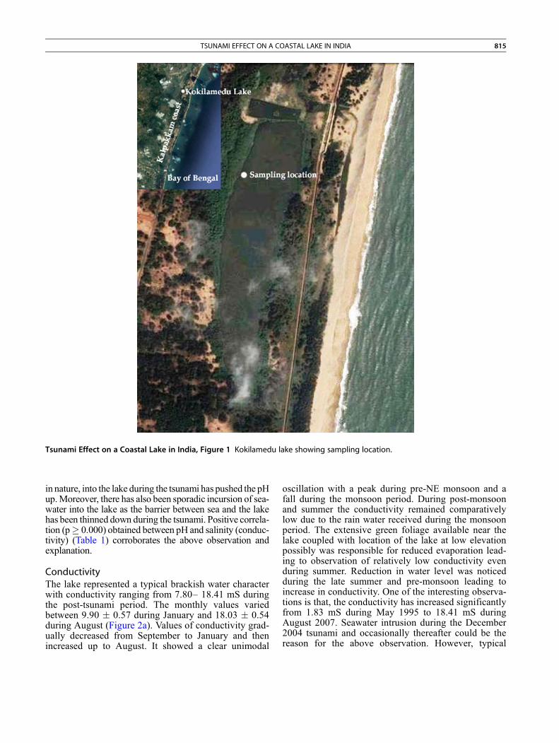
Tsunami Effect on a Coastal Lake in India, Figure 1 Kokilamedu lake showing sampling location.

TSUNAMI EFFECT ON A COASTAL LAKE IN INDIA 815

in nature, into the lake during the tsunami has pushed the pHup.Moreover, there has also been sporadic incursion of sea-water into the lake as the barrier between sea and the lakehas been thinned down during the tsunami. Positive correla-tion (p� 0.000) obtained between pH and salinity (conduc-tivity) (Table 1) corroborates the above observation andexplanation.

ConductivityThe lake represented a typical brackish water characterwith conductivity ranging from 7.80– 18.41 mS duringthe post-tsunami period. The monthly values variedbetween 9.90 � 0.57 during January and 18.03 � 0.54during August (Figure 2a). Values of conductivity grad-ually decreased from September to January and thenincreased up to August. It showed a clear unimodal

oscillation with a peak during pre-NE monsoon and afall during the monsoon period. During post-monsoonand summer the conductivity remained comparativelylow due to the rain water received during the monsoonperiod. The extensive green foliage available near thelake coupled with location of the lake at low elevationpossibly was responsible for reduced evaporation lead-ing to observation of relatively low conductivity evenduring summer. Reduction in water level was noticedduring the late summer and pre-monsoon leading toincrease in conductivity. One of the interesting observa-tions is that, the conductivity has increased significantlyfrom 1.83 mS during May 1995 to 18.41 mS duringAugust 2007. Seawater intrusion during the December2004 tsunami and occasionally thereafter could be thereason for the above observation. However, typical

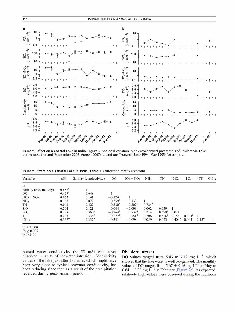
Tsunami Effect on a Coastal Lake in India, Table 1 Correlation matrix (Pearson)

Variables pH Salinity (conductivity) DO NO2 + NO3 NH3 TN SiO4 PO4 TP Chl-a

pH 1Salinity (conductivity) 0.688a 1DO �0.427a �0.648a 1NO2 + NO3 0.063 0.141 �0.124 1NH3 �0.167 0.077 �0.359b �0.133 1TN 0.043 0.422a �0.380a 0.302b 0.724a 1SiO4 0.204 0.121 0.044 �0.098 0.062 0.039 1PO4 0.178 0.360b �0.264c 0.739a 0.214 0.599a 0.011 1TP 0.203 0.335b �0.277c 0.751a 0.206 0.526a 0.154 0.884a 1Chl-a 0.367b 0.337b �0.341b �0.098 0.059 �0.023 0.404a 0.044 0.157 1

ap � 0.000bp � 0.005cp � 0.01

Sep-0

6

Oct-0

6

Nov-06

Dec-0

6

Jan-0

7

Feb-0

7

Mar

-07

Apr-0

7

May-0

7

Jun-0

7

Jul-0

7

Aug-07

7.27.88.49.0

pH

05

1015

Con

duct

ivity

(mS

)

3.04.56.07.5

DO

(mg

l−1)

0.11

10

NO

2+N

O3

(µ m

ol l−1

)

10

100

SiO

4(µ

mol

l−1)

0.1

1

10a b

PO

4(µ

mol

l−1)

pHC

ondu

ctiv

ity(m

S)

DO

(mg

l−1)

NO

2+N

O3

(µ m

ol l−1

)S

iO4

(µ m

ol l−1

)P

O4

(µ m

ol l−1

)

Jun-9

4

Jul-9

4

Aug-94

Sep-9

4

Oct-9

4

Dec-9

4

Jan-9

5

Feb-9

5

Mar-9

5

May-9

5 --

Jun-9

6

7.27.88.49.0

05

1015

3.04.56.07.5

0.1

1

10

10

100

0.1

1

10

Tsunami Effect on a Coastal Lake in India, Figure 2 Seasonal variation in physicochemical parameters of Kokilamedu Lakeduring post-tsunami (September 2006–August 2007) (a) and pre-Tsunami (June 1994–May 1995) (b) periods.

816 TSUNAMI EFFECT ON A COASTAL LAKE IN INDIA

coastal water conductivity ( 55 mS) was neverobserved in spite of seawater intrusion. Conductivityvalues of the lake just after Tsunami, which might havebeen very close to typical seawater conductivity, hasbeen reducing since then as a result of the precipitationreceived during post-tsunami period.

Dissolved oxygenDO values ranged from 5.43 to 7.12 mg L�1, whichshowed that the lake water is well oxygenated. The monthlyvalues of DO ranged from 5.67 � 0.16 mg L�1 in May to6.84 � 0.20 mg L�1 in February (Figure 2a). As expected,relatively high values were observed during the monsoon

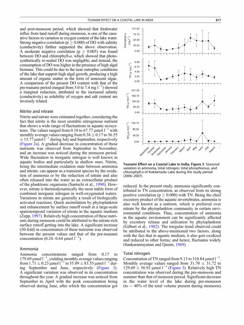
Septe

mbe

r

Octobe

r

Novem

ber

Decem

ber

Janu

ary

Febr

uary

Mar

chApr

ilM

ayJu

ne July

Augus

t

0.00

40.25

80.50

120.75

NH

3 (µ

mol

l–1)

0.00

60.25

120.50

180.75

241.00

TN

(µ

mol

l–1)

0.00

2.25

4.50

6.75

9.00

TP

(µ

mol

l–1)

0.00

25.25

50.50

75.75

101.00

Chl

orop

hyll-a

(mg

l–1)

Tsunami Effect on a Coastal Lake in India, Figure 3 Seasonalvariation in ammonia, total nitrogen, total phosphorous, andchlorophyll-a of Kokilamedu Lake during the study period(2006–2007).

TSUNAMI EFFECT ON A COASTAL LAKE IN INDIA 817

and post-monsoon period, which showed that freshwaterinflux from land runoff during monsoon, is one of the caus-ative factors in variation in oxygen content of the lake water.Strong negative correlation (p� 0.000) of DO with salinity(conductivity) further supported the above observation.A moderate negative correlation (p � 0.005) was foundbetween DO and chlorophyll-a, which showed that photo-synthetically re-sealed DO was negligible, and instead, theconsumption of DOwas higher in the presence of high algalbiomass. This could be due to the near eutrophic conditionsof the lake that support high algal growth, producing a highamount of organic matter in the form of senescent algae.A comparison of the present DO content with that of thepre-tsunami period (ranged from 5.0 to 7.4 mg l�1) showeda marginal reduction, attributed to the increased salinity(conductivity) as solubility of oxygen and salt content areinversely related.

Nitrite and nitrateNitrite and nitrate were estimated together, considering thefact that nitrite is the most unstable nitrogenous nutrientthat shows a wide range of fluctuations in aquatic ecosys-tems. The values ranged from 0.10 to 67.77 mmol l�1 withmonthly average values ranging from 0.38� 0.17 to 36.55� 15.77 mmol l�1 during July and September, respectively(Figure 2a). A gradual decrease in concentration of thesenutrients was observed from September to November,and an increase was noticed during the monsoon period.Wide fluctuation in inorganic nitrogen is well known inaquatic bodies and particularly in shallow ones. Nitrite,being the intermediate oxidation state between ammoniaand nitrate, can appear as a transient species by the oxida-tion of ammonia or by the reduction of nitrate and alsooften released into the water as an extracellular productof the planktonic organisms (Santschi et al., 1990). How-ever, nitrate is thermodynamically the most stable form ofcombined inorganic nitrogen in well-oxygenated waters.Variations in nitrate are generally a result of biologicallyactivated reactions. Quick assimilation by phytoplanktonand enhancement by surface runoff result in a large-scalespatiotemporal variation of nitrate in the aquatic medium(Zepp, 1997). Relatively high concentration of these nutri-ents during monsoon could be attributed to the nitrate-richsurface runoff getting into the lake. A significant increase(50-fold) in concentration of these nutrients was observedbetween the present values and that of the pre-tsunamiconcentration (0.24–0.64 mmol l�1).

AmmoniaAmmonia concentrations ranged from 0.17 to179.69 mmol l�1, yieldingmonthly average values rangingfrom 1.71� 0.23 mmol l�1 to 55.89� 83.55 mmol l�1 dur-ing September and June, respectively (Figure 3).A significant variation was observed in its concentrationthroughout the year. A gradual increase was noticed fromSeptember to April with the peak concentration beingobserved during June, after which the concentration got

reduced. In the present study, ammonia significantly con-tributed to TN concentration, as observed from its strongpositive correlation (p � 0.000) with TN. Being the chiefexcretory product of the aquatic invertebrates, ammonia isalso well known as a nutrient, which is preferred overnitrate by the phytoplankton community in certain envi-ronmental conditions. Thus, concentration of ammoniain the aquatic environment can be significantly affectedby excretory release and utilization by phytoplankton(Gilbert et al., 1982). The irregular trend observed couldbe attributed to the above-mentioned two factors, alongwith the fact that in aquatic medium, it also gets oxidizedand reduced to other forms; and hence, fluctuates widely(Sankaranrayanan and Qasim, 1969).

Total nitrogenConcentration of TN ranged from 9.13 to 310.84 mmol l�1.Monthly average values ranged from 31.70 � 31.72 to129.69 � 56.93 mmol l�1 (Figure 3). Relatively high TNconcentration was observed during the pre-monsoon andsummer than that of monsoon period. Significant decreasein the water level of the lake during pre-monsoon(to 40% of the total volume present during monsoon)

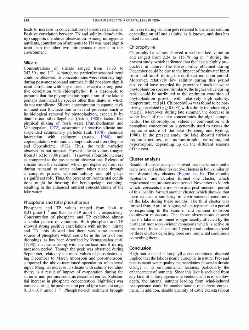
818 TSUNAMI EFFECT ON A COASTAL LAKE IN INDIA

leads to increase in concentration of dissolved nutrients.Positive correlation between TN and salinity (conductiv-ity) supports the above observation. Among nitrogenousnutrients, contribution of ammonia to TNwasmore signif-icant than the other two nitrogenous nutrients in thisenvironment.

SilicateConcentrations of silicate ranged from 17.33 to247.50 mmol l�1. Although no particular seasonal trendcould be observed, its concentrations were relatively highduring post-monsoon and summer. It did not show signif-icant correlation with any nutrients except a strong posi-tive correlation with chlorophyll-a. It is reasonable topresume that the phytoplankton population of the lake isperhaps dominated by species other than diatoms, whichdo not use silicate. Silicate concentration in aquatic envi-ronment can fluctuate due to several processes such asits biological removal by phytoplankton, especially bydiatoms and silicoflagellates (Aston, 1980); factors likephysical mixing of fresh water (Purushothaman andVenugopalan, 1972); adsorption of reactive silicate intosuspended sedimentary particles (Lal, 1978); chemicalinteraction with sediment (Aston, 1980); andcoprecipitation with humic compounds and iron (Stephnsand Oppenheime, 1972). Thus, the wide variationobserved is not unusual. Present silicate values (rangedfrom 37.62 to 78.86 mmol l�1) showed a fourfold increaseas compared to the pre-tsunami observations. Release ofsilicate from the sediment which got deposited from seaduring tsunami to water column takes place througha complex process wherein salinity and pH playsa significant role. Thus, the present environmental condi-tions might be favoring the benthopelagic coupling,resulting in the enhanced nutrient concentrations of thelake water.

Phosphate and total phosphorousPhosphate and TP values ranged from 0.46 to8.31 mmol l�1 and 0.55 to 9.59 mmol l�1, respectively.Concentration of phosphate and TP exhibited almosta similar pattern of variations. Both phosphate and TPshowed strong positive correlations with nitrite + nitrateand TN; this showed that there was some externalsource of phosphate which could be in the form of birddroppings, as has been described by Venugopalan et al.(1998), that came along with the surface runoff duringmonsoon period. Though the peak was observed duringSeptember, relatively increased values of phosphate dur-ing December to March (monsoon and post-monsoon)supported the above-mentioned speculation of externalinput. Marginal increase in silicate with salinity (conduc-tivity) is a result of impact of evaporation during thesummer and pre-monsoon, as described earlier. Substan-tial increase in phosphate concentration (eightfold) wasnoticed during the post-tsunami period (pre-tsunami range0.13–1.09 mmol l�1). Phosphate-rich sediment brought

from sea during tsunami gets released to the water columndepending on pH and salinity, as is known, and thus hashiked its content.

Chlorophyll-aChlorophyll-a values showed a well-marked variationand ranged from 2.24 to 115.78 mg m�3 during thepresent study, which indicated that the lake is highly pro-ductive in nature. The lowest value obtained duringDecember could be due to the impact of freshwater inputfrom land runoff during the northeast monsoon period.Moreover, relatively low salinity during this periodalso could have retarded the growth of brackish waterphytoplankton species. Similarly, the higher value duringApril could be attributed to the optimum condition ofphytoplankton growth with relatively high salinity,temperature, and pH. Chlorophyll-awas found to be pos-itively correlated (p� 0.005) with salinity (conductivity)and pH. Moreover, during late summer, the decrease inwater level of the lake concentrates the algal compo-nents. The chlorophyll-a values in combination withphosphate concentration is generally used to assess thetrophic structure of the lake (Forsberg and Ryding,1980). In the present study, the lake showed varioustrophic structures, such as mesotrophic, eutrophic, andhypertrophic, depending up on the different seasonsof the year.

Cluster analysisResults of cluster analysis showed that the same monthswere involved in their respective clusters in both similarityand dissimilarity clusters (Figure 4a, b). The monthsSeptember and October formed one cluster, whichrepresented the pre-monsoon period. November to Marchwhich represents the monsoon and post-monsoon periodof this locality formed another cluster, which showed thatthere existed a similarity in environmental conditionsof the lake during these months. The third cluster wasformed from April to August, which represented a periodcorresponding to the summer and summer monsoon(southwest monsoon). The above observations showedthat the lake environment is significantly affected by thenortheast monsoon (winter monsoon) which is active inthis part of India. The entire 1-year period is characterizedby three clusters depicting three environmental conditionscoinciding them.

ConclusionHigh nutrient and chlorophyll-a concentrations observedimplied that the lake is nearly eutrophic in nature. Pre- andpost-tsunami water quality characteristics showed a drasticchange in its environmental features, particularly theenhancement of nutrients. Since this lake is secluded fromany kind of anthropogenic interventions and is of shallowdepth, the internal nutrient loading from wind-inducedresuspension could be another source of nutrient enrich-ment. In addition, sizable quantity of cattle excreta (about

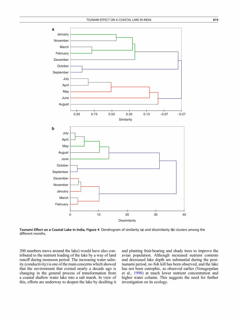
January

November

March

February

December

October

September

July

April

May

June

August

−0.27−0.070.130.330.530.730.93

Similarity

July

April

May

August

June

October

September

December

November

January

March

February

0 10 20 30 40

Dissimilarity

a

b

Tsunami Effect on a Coastal Lake in India, Figure 4 Dendrogram of similarity (a) and dissimilarity (b) clusters among thedifferent months.

TSUNAMI EFFECT ON A COASTAL LAKE IN INDIA 819

200 numbers move around the lake) would have also con-tributed to the nutrient loading of the lake by a way of landrunoff during monsoon period. The increasing water salin-ity (conductivity) is one of themain concernswhich showedthat the environment that existed nearly a decade ago ischanging in the general process of transformation froma coastal shallow water lake into a salt marsh. In view ofthis, efforts are underway to deepen the lake by desilting it

and planting fruit-bearing and shady trees to improve theavian population. Although increased nutrient contentsand decreased lake depth are substantial during the post-tsunami period, no fish kill has been observed, and the lakehas not been eutrophic, as observed earlier (Venugopalanet al., 1998) at much lower nutrient concentration andhigher water column. This suggests the need for furtherinvestigation on its ecology.

820 TURBIDITY CURRENTS IN RESERVOIRS

BibliographyAston, S. R., 1980. Nutrients dissolved gasses and general biochem-

istry in estuaries. In Olausson, E., and Cato, I. (eds.), Chemistryand Biogeochemistry of Estuaries. New York: Wiley,pp. 233–262.

Gilbert, P. M., Biggs, D. C., andMcCarthy, J. J., 1982. Utilization ofammonium and nitrate during austral summer in the Scotia sea.Deep Sea Research, 29, 837–850.

Grasshoff, K., Ehrhardt, M., and Kremling, K., 1983. Methods ofSeawater Analysis. New York: Wiley-VCH.

Lal, D., 1978. Transfer of chemical species through estuaries tooceans. In Proceedings of a UNESCO/SCOR Workshop on Bio-geochemistry of Estuarine Sediments. Melreus, Belgium,pp. 166–170.

Parsons, T. R., Maita, Y., and Lalli, C. M., 1984. AManual of Chem-ical and Biological Methods for Seawater Analysis. New York:Pergamon.

Purushothaman, A., and Venugopalan, V. K., 1972. Distribution ofdissolved Silicon in the Vellar Estuary. Indian Journal of MarineSciences, 1, 103–105.

Sankaranrayanan, V. N., and Qasim, S. Z., 1969. Nutrients of theCochin Backwaters in relation to environmental characteristics.Marine Biology, 2, 236–247.

Santschi, P., Honener, P., Benoit, G., and Brink, M. B., 1990. Chem-ical process at the sediment–water interface. Marine Chemistry,30, 269–315.

Satpathy, K. K., Mohanty, A. K., Prasad, M. V. R., Bhaskar S.,Jebakumar, K. E., 2007. Limnological studies in a freshwaterlake present in the vicinity of Kalpakkam coast, Tamil Nadu.In Proceedings of Taal 2007: 12th World Lake Conference.Rajasthan, India, pp. 1672–1678.

Satpathy, K. K., Mohanty, A. K., Prasad, M. V. R., 2008.A comparative account of water quality characteristics betweenpre- and post-Tsunami periods in a coastal brackish water lake.In Proceedings of 11th International Conference onWetland Sys-tems for Water Pollution Control. Ujjaian, India, pp. 627–633.

Stephns, C., Oppenheime, C. H., 1972. Silica contents in theNorthwestern Florida Gulf Coast. Marine Science, 16, 99–108.

Venugopalan, V. P., Nandakumar, K., Rajamohan, R., Sekar, R., andNair, K. V. K., 1998. Natural eutrophication and fish kill ina shallow freshwater lake. Current Science, 74, 915–917.

Zepp, R. G., 1997. Interactions of marine biogeochemical cyclesand the photodegradation of dissolved organic carbon anddissolved organic nitrogen. In Gianguzza, A., Pelizzetti, E.,and Sammarkano, S. (eds.),Marine Chemistry. London: Kluwer,pp. 329–352.

Cross-referencesCoastal Lagoons

TURBIDITY CURRENTS IN RESERVOIRS

Josef Schneider1, Gabriele Harb1, Hannes Badura21Institute of Hydraulic Engineering and WaterResources Management, Graz University of Technology,Graz, Austria2Verbund Hydro Power AG, Vienna, Austria

IntroductionImpounding and retaining water in reservoirs has been oneessential basic development for the onset of human civili-zation. An important aspect, though, which has been

known for a long time and which has lately gained inimportance, is reservoir sedimentation. Statistics showthat more than 50% of streams and rivers are dammed,which implies that the greater part of transportedsediment, in fact some 80%, is trapped in reservoirs. Thiscorresponds to a volume of about 8–16 km³ (Lemperierand and Lafitte, 2006). Morris and Fan (1998) quantifiedthe world’s total sediment deposit at between 15 and40 Gt p.a.; this corresponds to between 0.5 and 1 t ofsediment per 1,000 m³ of water. White (2001) estimatesthat more than 0.5% of the total reservoir storage volumeis lost worldwide due to reservoir sedimentation. Thecosts for restoring these losses and rebuilding the damscan be estimated at US$13 billion a year (Palmieriet al., 2003). Considering the different scales of reser-voirs, it can be stated that for small reservoirs, the sedi-ment budget can be managed within the framework ofthe operation rules and is considered as a routine job(e.g., water intakes). For reservoirs defined by greatcapacity with large dead-storage spaces, sedimentationis a long term rather than an acute phenomenon.The medium-sized reservoirs are characterized by sedi-mentation problems that need to be counteracted withadequate measures. Further, since these reservoirs areoften operated on a daily or weekly basis, the relativelysmall available storage is intensively utilized. The mostcommonly applied methodologies for handling reservoirsedimentation are dredging and flushing activities(Palmieri et al., 2003). Dredging is costly and spatiallya highly limited measure. Reservoir flushings are effec-tive, but may, in fact, have substantial ecological impacts.Increased sediment concentrations downstream of damsmay cause direct damage to fish populations and themacrozoobenthos while clogging off interstitial spacesin the gravel bed and evolving, thus, into substantiallong-term problems.

Density currentsThe force of gravity and small differences in density ofwater keep a density current in motion. In the case of lakesand reservoirs, the current is generated between differentparts of the same fluid.

The differences in density can be triggered by:

� Temperature� Salinity� Concentration of suspended sediment (turbidity)

Figure 1, beneath, is a satellite image showing themouth of the River Rhine in Lake Constance. Theplunge point area (1) is clearly visible, and the plung-ing density current proceeding in a north-western direc-tion from the mouth (2) is also clearly discernible.Schoklitsch (1935) described already the plunge ofthe River Rhine into Lake Constance, called “brech”by the local population, whereas that of the RiverRhône into Lake Geneva was locally termed “labataillière.”

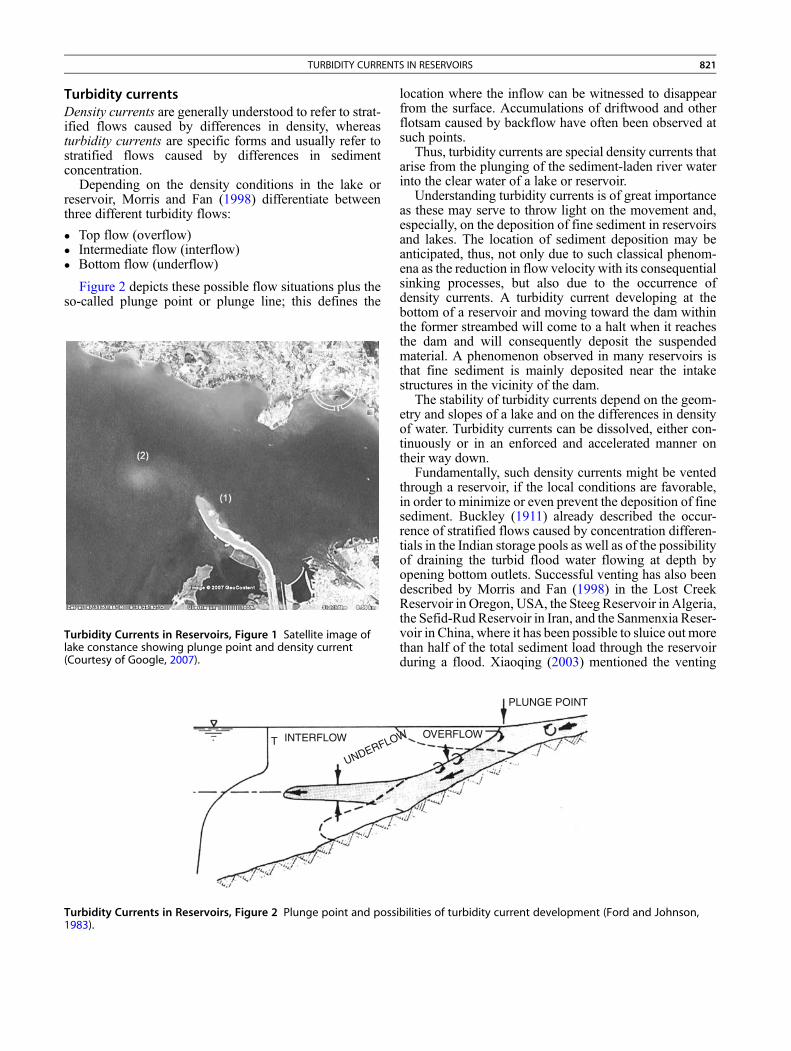
TURBIDITY CURRENTS IN RESERVOIRS 821

Turbidity currentsDensity currents are generally understood to refer to strat-ified flows caused by differences in density, whereasturbidity currents are specific forms and usually refer tostratified flows caused by differences in sedimentconcentration.

Depending on the density conditions in the lake orreservoir, Morris and Fan (1998) differentiate betweenthree different turbidity flows:

� Top flow (overflow)� Intermediate flow (interflow)� Bottom flow (underflow)

Figure 2 depicts these possible flow situations plus theso-called plunge point or plunge line; this defines the

Turbidity Currents in Reservoirs, Figure 1 Satellite image oflake constance showing plunge point and density current(Courtesy of Google, 2007).

INTERFLOWT

UNDERFLO

Turbidity Currents in Reservoirs, Figure 2 Plunge point and possi1983).

location where the inflow can be witnessed to disappearfrom the surface. Accumulations of driftwood and otherflotsam caused by backflow have often been observed atsuch points.

Thus, turbidity currents are special density currents thatarise from the plunging of the sediment-laden river waterinto the clear water of a lake or reservoir.

Understanding turbidity currents is of great importanceas these may serve to throw light on the movement and,especially, on the deposition of fine sediment in reservoirsand lakes. The location of sediment deposition may beanticipated, thus, not only due to such classical phenom-ena as the reduction in flow velocity with its consequentialsinking processes, but also due to the occurrence ofdensity currents. A turbidity current developing at thebottom of a reservoir and moving toward the dam withinthe former streambed will come to a halt when it reachesthe dam and will consequently deposit the suspendedmaterial. A phenomenon observed in many reservoirs isthat fine sediment is mainly deposited near the intakestructures in the vicinity of the dam.

The stability of turbidity currents depend on the geom-etry and slopes of a lake and on the differences in densityof water. Turbidity currents can be dissolved, either con-tinuously or in an enforced and accelerated manner ontheir way down.

Fundamentally, such density currents might be ventedthrough a reservoir, if the local conditions are favorable,in order to minimize or even prevent the deposition of finesediment. Buckley (1911) already described the occur-rence of stratified flows caused by concentration differen-tials in the Indian storage pools as well as of the possibilityof draining the turbid flood water flowing at depth byopening bottom outlets. Successful venting has also beendescribed by Morris and Fan (1998) in the Lost CreekReservoir in Oregon, USA, the Steeg Reservoir in Algeria,the Sefid-Rud Reservoir in Iran, and the Sanmenxia Reser-voir in China, where it has been possible to sluice out morethan half of the total sediment load through the reservoirduring a flood. Xiaoqing (2003) mentioned the venting

PLUNGE POINT

OVERFLOWW

bilities of turbidity current development (Ford and Johnson,

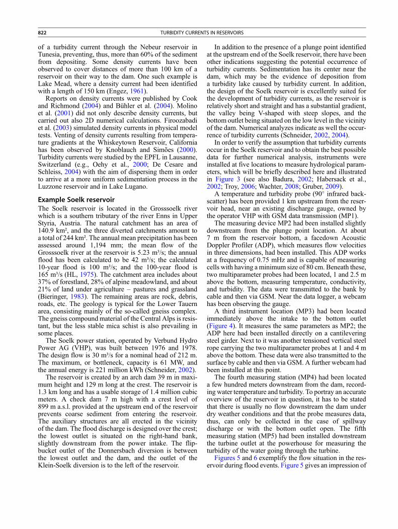
822 TURBIDITY CURRENTS IN RESERVOIRS

of a turbidity current through the Nebeur reservoir inTunesia, preventing, thus, more than 60% of the sedimentfrom depositing. Some density currents have beenobserved to cover distances of more than 100 km of areservoir on their way to the dam. One such example isLake Mead, where a density current had been identifiedwith a length of 150 km (Engez, 1961).

Reports on density currents were published by Cookand Richmond (2004) and Bühler et al. (2004). Molinoet al. (2001) did not only describe density currents, butcarried out also 2D numerical calculations. Firoozabadiet al. (2003) simulated density currents in physical modeltests. Venting of density currents resulting from tempera-ture gradients at the Whiskeytown Reservoir, Californiahas been observed by Knoblauch and Simões (2000).Turbidity currents were studied by the EPFL in Lausanne,Switzerland (e.g., Oehy et al., 2000; De Cesare andSchleiss, 2004) with the aim of dispersing them in orderto arrive at a more uniform sedimentation process in theLuzzone reservoir and in Lake Lugano.

Example Soelk reservoirThe Soelk reservoir is located in the Grosssoelk riverwhich is a southern tributary of the river Enns in UpperStyria, Austria. The natural catchment has an area of140.9 km², and the three diverted catchments amount toa total of 244 km². The annual mean precipitation has beenassessed around 1,194 mm; the mean flow of theGrosssoelk river at the reservoir is 5.23 m³/s; the annualflood has been calculated to be 42 m³/s; the calculated10-year flood is 100 m³/s; and the 100-year flood is165 m³/s (HL, 1975). The catchment area includes about37% of forestland, 28% of alpine meadowland, and about21% of land under agriculture – pastures and grassland(Bieringer, 1983). The remaining areas are rock, debris,roads, etc. The geology is typical for the Lower Tauernarea, consisting mainly of the so-called gneiss complex.The gneiss compoundmaterial of the Central Alps is resis-tant, but the less stable mica schist is also prevailing insome places.

The Soelk power station, operated by Verbund HydroPower AG (VHP), was built between 1976 and 1978.The design flow is 30 m³/s for a nominal head of 212 m.The maximum, or bottleneck, capacity is 61 MW, andthe annual energy is 221 million kWh (Schneider, 2002).

The reservoir is created by an arch dam 39 m in maxi-mum height and 129 m long at the crest. The reservoir is1.3 km long and has a usable storage of 1.4 million cubicmeters. A check dam 7 m high with a crest level of899 m a.s.l. provided at the upstream end of the reservoirprevents coarse sediment from entering the reservoir.The auxiliary structures are all erected in the vicinityof the dam. The flood discharge is designed over the crest;the lowest outlet is situated on the right-hand bank,slightly downstream from the power intake. The flip-bucket outlet of the Donnersbach diversion is betweenthe lowest outlet and the dam, and the outlet of theKlein-Soelk diversion is to the left of the reservoir.

In addition to the presence of a plunge point identifiedat the upstream end of the Soelk reservoir, there have beenother indications suggesting the potential occurrence ofturbidity currents. Sedimentation has its center near thedam, which may be the evidence of deposition froma turbidity lake caused by turbidity current. In addition,the design of the Soelk reservoir is excellently suited forthe development of turbidity currents, as the reservoir isrelatively short and straight and has a substantial gradient,the valley being V-shaped with steep slopes, and thebottom outlet being situated on the low level in the vicinityof the dam. Numerical analyzes indicate as well the occur-rence of turbidity currents (Schneider, 2002, 2004).

In order to verify the assumption that turbidity currentsoccur in the Soelk reservoir and to obtain the best possibledata for further numerical analysis, instruments wereinstalled at five locations to measure hydrological param-eters, which will be briefly described here and illustratedin Figure 3 (see also Badura, 2002; Habersack et al.,2002; Troy, 2006; Wachter, 2008; Gruber, 2009).

A temperature and turbidity probe (90� infrared back-scatter) has been provided 1 km upstream from the reser-voir head, near an existing discharge gauge, owned bythe operator VHP with GSM data transmission (MP1).

The measuring device MP2 had been installed slightlydownstream from the plunge point location. At about7 m from the reservoir bottom, a facedown AcousticDoppler Profiler (ADP), which measures flow velocitiesin three dimensions, had been installed. This ADP worksat a frequency of 0.75 mHz and is capable of measuringcells with having a minimum size of 80 cm. Beneath these,two multiparameter probes had been located, 1 and 2.5 mabove the bottom, measuring temperature, conductivity,and turbidity. The data were transmitted to the bank bycable and then via GSM. Near the data logger, a webcamhas been observing the gauge.

A third instrument location (MP3) had been locatedimmediately above the intake to the bottom outlet(Figure 4). It measures the same parameters as MP2; theADP here had been installed directly on a cantileveringsteel girder. Next to it was another tensioned vertical steelrope carrying the two multiparameter probes at 1 and 4 mabove the bottom. These data were also transmitted to thesurface by cable and then via GSM. A further webcam hadbeen installed at this point.

The fourth measuring station (MP4) had been locateda few hundred meters downstream from the dam, record-ing water temperature and turbidity. To portray an accurateoverview of the reservoir in question, it has to be statedthat there is usually no flow downstream the dam underdry weather conditions and that the probe measures data,thus, can only be collected in the case of spillwaydischarge or with the bottom outlet open. The fifthmeasuring station (MP5) had been installed downstreamthe turbine outlet at the powerhouse for measuring theturbidity of the water going through the turbine.

Figures 5 and 6 exemplify the flow situation in the res-ervoir during flood events. Figure 5 gives an impression of

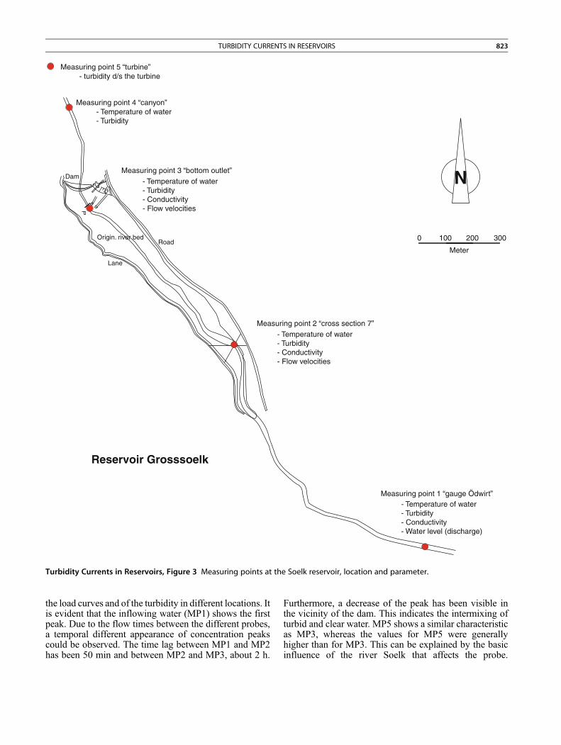
N

Measuring point 5 “turbine”- turbidity d/s the turbine

Measuring point 4 “canyon”

Measuring point 3 “bottom outlet”

Measuring point 2 “cross section 7”

Measuring point 1 “gauge Ödwirt”

- Temperature of water- Turbidity

- Temperature of water- Turbidity - Conductivity - Flow velocities

- Temperature of water- Turbidity - Conductivity - Flow velocities

- Temperature of water- Turbidity - Conductivity - Water level (discharge)

0 100 200 300

Meter

Dam

Lane

Origin. river bedRoad

Reservoir Grosssoelk

Turbidity Currents in Reservoirs, Figure 3 Measuring points at the Soelk reservoir, location and parameter.

TURBIDITY CURRENTS IN RESERVOIRS 823

the load curves and of the turbidity in different locations. Itis evident that the inflowing water (MP1) shows the firstpeak. Due to the flow times between the different probes,a temporal different appearance of concentration peakscould be observed. The time lag between MP1 and MP2has been 50 min and between MP2 and MP3, about 2 h.

Furthermore, a decrease of the peak has been visible inthe vicinity of the dam. This indicates the intermixing ofturbid and clear water. MP5 shows a similar characteristicas MP3, whereas the values for MP5 were generallyhigher than for MP3. This can be explained by the basicinfluence of the river Soelk that affects the probe.

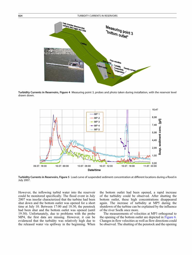
Turbidity Currents in Reservoirs, Figure 4 Measuring point 3, probes and photo taken during installation, with the reservoir leveldrawn down.

Turbidity Currents in Reservoirs, Figure 5 Load curve of suspended sediment concentration at different locations during a flood inJuly 2007.

824 TURBIDITY CURRENTS IN RESERVOIRS

However, the inflowing turbid water into the reservoircould be monitored specifically. The flood event in July2007 was insofar characterized that the turbine had beenshut down and the bottom outlet was opened for a shorttime at July 10. Between 17:00 and 18:30, the penstockhad been shut and the bottom outlet was opened (until19:30). Unfortunately, due to problems with the probeMP4, the first data are missing. However, it can beevidenced that the turbidity was relatively high due tothe released water via spillway in the beginning. When

the bottom outlet had been opened, a rapid increaseof the turbidity could be observed. After shutting thebottom outlet, these high concentrations disappearedagain. The increase of turbidity at MP5 during theshutdown of the turbine can be explained by the influenceof the river Soelk once more.

The measurements of velocities at MP3 orthogonal tothe opening of the bottom outlet are depicted in Figure 6.Changes in flow velocities as well as flow directions couldbe observed. The shutting of the penstock and the opening

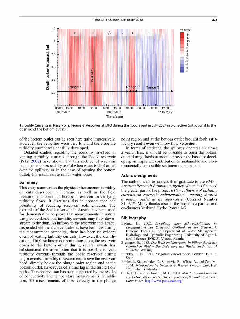
Turbidity Currents in Reservoirs, Figure 6 Velocities at MP3 during the flood event in July 2007 in y-direction (orthogonal to theopening of the bottom outlet).

TURBIDITY CURRENTS IN RESERVOIRS 825

of the bottom outlet can be seen here quite impressively.However, the velocities were very low and therefore theturbidity current was not fully developed.

Detailed studies regarding the economy involved inventing turbidity currents through the Soelk reservoir(Putz, 2007) have shown that this method of reservoirmanagement is especially useful when water is dischargedover the spillway as in the case of opening the bottomoutlet; this entails not to minor water losses.

SummaryThis entry summarizes the physical phenomenon turbiditycurrents described in literature as well as the fieldmeasurements taken in a European reservoir for verifyingturbidity flows. It discusses also in consequence onepossibility of reducing reservoir sedimentation. Theexample of the Soelk reservoir in Austria has been usedfor demonstration to prove that measurements in naturecan give evidence that turbidity currents may flow down-stream to the dam. As inflows to the reservoir and, hence,suspended sediment concentrations, have been low duringthe measurement campaign, there has been no evidentevent of venting turbidity currents. However, the identifi-cation of high sediment concentrations along the reservoirdown to the bottom outlet during several events hassubstantiated the assumption that it is possible to ventturbidity currents through the Soelk reservoir duringmajor events. Turbidity measurements above the reservoirhead, directly below the plunge point region and at thebottom outlet, have revealed a time lag in the turbid flowpeaks. This observation has been supported by the resultsof conductivity and temperature measurements. In addi-tion, 3D measurements of flow velocity in the plunge

point region and at the bottom outlet brought forth satis-factory results even with low flow velocities.

In terms of statistics, the spillway operates six timesa year. Thus, it should be possible to open the bottomoutlet during floods in order to provide the basis for devel-oping an important contribution to sustainable and envi-ronmentally compatible sediment management.

Acknowledgments

The authors wish to express their gratitude to the FFG –Austrian Research Promotion Agency, which has financedthe greater part of the project ETS – Influence of turbiditycurrents on reservoir sedimentation – venting througha bottom outlet as an alternative (Contract Number810977). Many thanks also to the economic partner andco-financer Verbund Hydro Power AG.

BibliographyBadura, H., 2002. Erstellung einer Schwebstoffbilanz im

Einzugsgebiet des Speichers Großsölk in der Steiermark.Diploma Thesis at the Department of Water Management,Hydrology and Hydraulic Engineering, University of Agricul-tural Sciences (BOKU), Vienna, Austria.

Bieringer, B., 1983. Der Wald im Naturpark. In Führer durch denheimischen Wald – Die Bedeutung des Waldes im NaturparkSölktäler, Walling.

Buckley, R. B., 1911. Irrigation Pocket Book. London: E. u. F.Spon.

Bühler, J., Siegenthaler, C., Simitovic, R., Wüest, A., and Zeh, M.,2004. Trübeströme im Grimselsee, Wasser, Energie, Luft, Heft5/6, Baden, Switzerland.

Cook, C. B., and Richmond, M. C., 2004.Monitoring and simulat-ing 3-D density currents at the confluence of the snake and clear-water rivers, http://www.pubs.asce.org/.

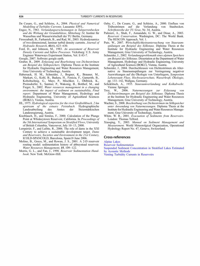
826 TURBIDITY CURRENTS IN RESERVOIRS

De Cesare, G., and Schleiss, A., 2004. Physical and NumericalModelling of Turbidity Currents. Lausanne: EPFL.

Engez, N., 1961. Verlandungserscheinungen in Talsperrenbeckenund die Wirkung der Grundablässe, Mitteilung 54, Institut fürWasserbau und Wasserwirtschaft der TU Berlin, Germany.

Firoozabadi, B., Farhanieh, B., and Rad, M., 2003. Hydrodynamicsof two-dimensional, laminar turbid density currents. Journal ofHydraulic Research, 41(6), 623–630.

Ford, D., and Johnson, M., 1983. An assessment of ReservoirDensity Currents and Inflow Processes. Vicksburg: U.S. ArmyEngineer Waterways Experiment Station, Vol. E-83-7.

Google, 2007. Software google earth.Gruber, R., 2009. Erfassung und Bearbeitung von Dichteströmen

am Beispiel des Sölkspeichers. Diploma Thesis at the Institutefor Hydraulic Engineering and Water Resources Management,Graz University of Technology, Austria.

Habersack, H. M., Schneider, J., Bogner, K., Brauner, M.,Markart, G., Kohl, B., Badura, H., Fenicia, F., Gamerith, B.,Koboltschnig, G., Mayr, P., Mischker, J., Öhlböck, K.,Preinsdorfer, S., Santner, P., Wakonig, B., Botthof, M., andFieger, S., 2002. Water resources management in a changingenvironment: the impact of sediment on sustainability, Finalreport. Department of Water Management, Hydrology andHydraulic Engineering, University of Agricultural Sciences(BOKU), Vienna, Austria.

HL, 1975. Hydrological expertise for the river Großsölkbach, 2 kmupstream of the estuary Feistabach. HydrographischeLandesabteilung des Amtes der SteiermärkischenLandesregierung, Austria.

Knoblauch, H., and Simões, F., 2000. Calculation of the PlungePoint at Whiskeytown Reservoir, California. In Proceedings ofthe 5th International Symposium on Stratified Flows, Universityof British Columbia, Vancouver, July 10–13, 2000.

Lempérièr, F., and Lafitte, R., 2006. The role of dams in the XXICentury to achieve a sustainable development target. Damsand Reservoirs, Societies and Environment in the 21st Century,ICOLD-SPANCOLD, Barcelona, Spain18 June 2006.

Molino, B., Greco, M., and Rowan, J. S., 2001. A 2-D reservoirrouting model: sedimentation history of abbeystead reservoir.Water Resources Management, 15, 109–122.

Morris, G. L., and Fan, J., 1998. Reservoir Sedimentation Hand-book. New York: McGraw-Hill.

Oehy, C., De Cesare, G., and Schleiss, A., 2000. Einfluss vonTrübeströmen auf die Verlandung von Staubecken.Schriftenreihe der TU Graz, Nr. 34, Austria.

Palmieri, A., Shah, F., Annandale, G. W., and Dinar, A., 2003.Reservoir Conservation. Washington, DC: The World Bank.The RESCON Approach, Vol. 1.

Putz, W., 2007. Wirtschaftlichkeitsuntersuchung von Stauraum-spülungen am Beispiel des Sölkstaus. Diploma Thesis at theInstitute for Hydraulic Engineering and Water ResourcesManagement, Graz University of Technology, Austria.

Schneider, J., 2002. Verlandungsproblematik eines alpinen Speichersam Beispiel des Sölkstaus.Dissertation at the Department of WaterManagement, Hydrology and Hydraulic Engineering, Universityof Agricultural Sciences (BOKU), Vienna, Austria.

Schneider, J., 2004. Durchschleusen von Dichteströmen als Alter-native zu Stauraumspülungen zur Verringerung negativerAuswirkungen auf die Ökologie von Unterliegern, SymposiumLebensraum Fluss, Hochwasserschutz, Wasserkraft, Ökologie,pp. 133–142, Wallgau, Germany.

Schoklitsch, A., 1935. Stauraumverlandung und Kolkabwehr.Vienna: Springer.

Troy, W., 2006. Naturmessungen zur Erfassung vonDichteströmungen am Beispiel des Sölkstaus. Diploma Thesisat the Institute for Hydraulic Engineering and Water ResourcesManagement, Graz University of Technology, Austria.

Wachter, S., 2008. Beschreibung von Dichteströmen im Sölkspeicherunter Anwendung von Naturmessungen. Diploma Thesis at theInstitute for Hydraulic Engineering andWater ResourcesManage-ment, Graz University of Technology, Austria.

White, W. R., 2001. Evacuation of Sediments from Reservoirs.London: Thomas Telford.

Xiaoqing, Y., 2003. Manual on Sediment Management andMeasurement. World Meteorolgical Organization, OperationalHydrology Report No. 47, Geneve, Switzerland.

Cross-referencesAlpine LakesReservoir SedimentationSuspended Sediment Concentration in Stratified Lakes Estimatedby Acoustic MethodsVenting Turbidity Currents in Reservoirs