Twenty-four hour predictions of f 0 F 2 using time delay neural networks

Radio Science, Volume 35, Number 2, Pages 395-408, March-April 2000

Twenty-four hour predictions of foF: using time delay neural networks

Peter Wintoft

Solar-Terrestrial Physics Division, Swedish Institute of Space Physics, Lund, Sweden

Ljiljana R. Cander CLRC Rutherford Appleton Laboratory, Chilton, Didcot, Oxon, England, United Kingdom

Abstract. The use of time delay feed-forward neural networks to predict the hourly values of the ionospheric F2 layer critical frequency, foF2, 24 hours ahead, have been examined. The 24 measurements of foF2 per day are reduced to five coefficients with principal component analysis. A time delay line of these coefficients is then used as input to a feed-forward neural network. Also included in the input are the 10.7 cm solar flux and the geomagnetic index Ap. The network is trained to predict measured foF2 data from 1965 to 1985 at Slough ionospheric station and validated on an independent validation set from the same station for the periods 1987-1990 and 1992-1994. The results are compared with two different autocorrelation methods for the years 1986 and 1991, which correspond to low and high solar activity, respectively.

1. Introduction

Ionospheric prediction and forecasting is an issue for a wide range of communication and navigation system users. The planning and frequency manage- ment of HF radio systems, HF automatic link estab- lishment, global positioning satellites, and HF and UHF radars are all affected by the ionospheric conditions. Predictions in practical applications, whether short or long term, that should be quantitative and run in real time, require fast and robust techniques that should capture many of the rather complex temporal and spatial variations of key ionospheric parameters. The problem and related phenomena have been studied by several workers for many years [Mc- Namara, 1991; Goodman, 1992; Johnson et al., 1997; and references therein]. In a series of papers based on observations and modeling, traditional methods were used to predict the key ionospheric parameters (F•, F1 and E region peaks) [Houminer and Soicher, 1996; Heckman et al., 1997; and references

Copyright 2000 by the American Geophysical Union.

Paper number 1998RS002149. 0048-6604 / 00 / 1998RS 002149511.00

therein]. However, an efficient prediction tool is still missing. This is particularly true for those applications of ionospheric predictions involving timescales of less than a month.

Our approach here is to introduce an artificial neural network, combined with principal component analysis, to predict the ionospheric parameter foF2 24 hours ahead. The short-term (hourly) variation of foF2 has been studied extensively using neural networks. Models for 1-hour-ahead predictions have been developed by a number of people [Altinay et al., 1997; Cander and Lamming, 1997; Cander et al., 1998; Wintort and Cander, 1999a; Kumluca et al., 1999]. Other studies concentrate on predicting the noon foF2 value [Williscroft and Poole, 1996; Fran- cis et al., 1998; Poole and McKinnel, 1998]. Finally, on these timescales, efforts have been made to predict foF2 up to 24-30 hours ahead [Francis et al., 1999a, b]. There is also a model for the prediction of the monthly median foF2 several months ahead [Lamming and Cander, 1999]. All the models share a common architecture in that they use past values of foF2 as input. In addition, some models also contain information about solar activity (sunspot number or 10.7 cm radio flux), geomagnetic activity (AE, Dst, Kp, Ap), or time (season, local time). The ca-

395

3!)•i WINTOFT AND CANDER: TWENTY-FOUR HOUR PREDICTIONS OF loft.

pability of successful foF2 forecasting 1 hour ahead at Slough and Rome ionospheric stations [Cander et al., 1998; Wintort and Cander, 1999a] has provided a unique opportunity to study the role of artificial neural networks in the prediction of foF2 a few days ahead covering both quiet and disturbed ionospheric conditions. A modular neural network has already given a very realistic foF2 representation in long-term prediction of the monthly median foF2 values at single midlatitude ionospheric stations and over the region of Europe delimited by 35 ø - 70øN, 10øW- 60øE [Lamming and Cander, 1999]. The new method has been compared to traditional autocorrelation methods for the quiet ionosphere as described by Muhtarov and Kutiev [1999] and Kutiev et al. [1999]. This paper outlines the background of the problem, explains the neural network approach, gives the results with comparison to existing prediction techniques, and discusses the implementation in real-time mode. It is also shown that an artificial

neural network is a valuable tool for investigating the ionospheric structure at a single location when longer periods of the ionospheric measurements are missing.

2. Motivation for Neural Networks

in Ionospheric Predictions The Earth's ionosphere, which reflects radio waves

to long distances and modifies the propagation of satellite signals, has been studied since about 1935 using vertical incidence sounding by sweep frequency ionosondes. Since then, bottom side and topside ionosondes have become a basic tool for ionospheric research. They generally scan from I to 20 MHz, transmitting modulated radio waves and receiving and analyzing the ionospherically reflected echo signals [Reinisch, 1996]. An ionogram, the output of an ionosonde, is a graph of time of flight against transmitted frequency which can be analyzed to give the variation of electron density with height up to the peak of the ionosphere. The radio frequency reflected at the maximum electron density in a given ionospheric layer at vertical incidence is called the critical frequency for the ordinary wave, fo. The ordinary wave critical frequency of the highest stratification in the F region, the F• layer, is called the critical frequency, loft. Parameters such as electron density profiles and the critical frequency of the F2 layer provide most of the information required for studies

of the ionosphere and its effect on radio communications. However, an ionogram can be much more complicated than just one or two layers [Piggott and Rawer, 1972]. There can also be such phenomena as the following: the F1 layer (an additional layer which appears in the F region, between the two existing peaks); sporadic E, Es layer (a patchy, very dense layer often exceeding 16 MHz); D region ab- sorption (caused by ionization in the D region that absorbs the transmitted wave before it can return to

the ground); lacuna (when turbulence occurs, as the result of large electric fields, for example, the strat- ified nature of the ionosphere gives way to a more complex structure); and spread F (multiple traces on an ionogram because of different horizontal posi- tion of each echo).

Apart from the ionospheric variations with height, leading to the different layers, the ionosphere varies significantly throughout the day and season and with location and solar activity (Figure 1). All these variations are part of the F2 layer dynamics and must be taken into account in order to predict and forecast foF2 changes successfully. The variations are the manifestation of complex interactions between neu- tral and ionized constituents, dependence of the F2 layer phenomena upon the geomagnetic field, and the influence of the magnetosphere on the ionosphere. The diurnal variation of foF2 reaches its lowest values just before dawn, then exhibits a rapid rise during morning and a sharp decrease during evening. A typical F2 layer maximum electron density of 1012 electrons/m 3 corresponds to a critical frequency of 9 MHz (see Figure 1). The critical frequency varies throughout the year with season. This unexpected variation has its maximum during summer months and is caused by the seasonal changes in the relative concentrations of ionospheric atomic and molecular species [Davies, 1990]. The midlatitude seasonal anomaly is a well-known feature, and it is clearly seen in Figure 1, where winter (December) values of foF2 during the day, at high levels of solar activity, exceed the equinox (September) values. The ionospheric F2 layer also varies significantly with geographic and geomagnetic locations. The extreme cases of the equa- torial and polar ionosphere are avoided here, as we only consider the prediction problem at the midlatitude station of Slough.

The solar cycle dependence of the F2 layer is fun- damental. This can be seen in Figure 1, which shows that from around solar maximum (1990) to around

WINTOFT AND CANDER: TWENTY-FOUR HOUR PREDICTIONS OF foF2 397

15

A

N 10

v

o

5

0 6

I I I I

Day in December

15

A

• 10 v

5

0 6

t i i i i i i i i i j

I - I1

• •.... _/ / \A,•.,, /! ' '• -... • I I k x • /; \\ 65 7 75 8 85 9 95 10 10.5 11

Day in September

Figure 1. Variations throughout a few days of the hourly critical frequency of the F2 layer foF2 at Slough for winter (December) and equinox (September) and for two levels of solar activity (high, 1990; low, 1994).

solar minimum (1994) there is a large variation in foF2. Values of foF2 in 1990 strongly exceed those in 1994. During intense periods of solar activity, giv- ing rise to major magnetospheric and ionospheric dis- turbances, the regular F2 layer structure and dynamics can be destroyed, creating positive (midlatitude winter) and negative (midlatitude summer) phases of ionospheric storms. The result of all changes during different phases of ionospheric storms is that the critical frequency in the F2 layer can be either increased or decreased (often by a factor of 2) depending on a number of things such as the time of day when the disturbance started, its intensity, the local time, the season, and the location of the observation points IRishbeth, 1991; PrSlss, 1995]. Ionospheric variation from day to day, or ionospheric space weather, is rather complicated because it cannot be linked di- rectly to any single solar-terrestrial event. It can be attributed to all the mentioned changes in the prime characteristics of the ionosphere. Accurate predictions with short lead times are most useful in view

of the lack of advance information on solar and geomagnetic parameters [Wilkinson et al., 1997].

Neural networks provide a practical method of modeling ionospheric variations because (1) they are

empirical models that can describe nonlinear phenomena strongly involved in the ionospheric variability, (2) they are trained on measured ionosonde data from which they extract the underlying func- tional relationships, and (3) they are fast enough that they can be used for real-time operation. The technique in its current state of development makes use of long time series of scaled foF2 values from ionograms and morphology of the ionospheric variations seen at Slough station, the 10.7 cm solar flux, and the Ap index to create the numerical prediction model of the most likely ionospheric conditions. A similar technique should be applicable to any other key ionospheric characteristics of vertical incidence, at any other midlatitude station, provided that long time series of data and sufficient morphological knowledge are available.

3. Database

We have used the published values of foF2 scaled from hourly ionograms from the midlatitude ionosonde situated at Slough (51.5øN, 0.6øW). The database extends over the years from 1965 up to and in- cluding 1994. Any data gaps of i or 2 hours have

398 WINTOFT AND CANDER: TWENTY-FOUR HOUR PREDICTIONS OF loft.

been replaced by linearly interpolated values. The data set was then divided into three different sets: a

training set, extending over the period 1965-1985; a validation set over the periods 1987-1990 and 1992- 1994; and a test set for the years 1986 and 1991. The total period covers the three latest solar cycles.

Also included in the data sets are the daily values of the 10.7 cm solar radio flux and the geomagnetic activity index Ap. The solar flux describes the solar activity variation which causes the large difference in the foF2 level as shown in Figure 1. The Ap index serves as a measure of the general level of geomagnetic activity which is related to the ionospheric storms.

4. Preprocessing of the Data

The feed-forward neural network, which we introduce in section 5, has no notion of time. Thus, to be able to capture the dynamics of a system, time has to be described at the network input. We solve this by transforming the temporal signal into a spatial pattern. Thus we construct a time delay vector that consists of the values of the time series from

time t- r to t, where t is current time and r is a number of hours back in time. The resulting net-

work is called a time delay neural network. In this study we use hourly foF2 data over 7 days for the time delay vector to predict the 24 hours of the next day. However, with the use of the time delay vector the number of inputs becomes large, which leads to long training times and generally poor network performance. To overcome this problem, we apply principal component analysis (PCA) [Jolliffe, 1986] to reduce the dimension of the foF2 input vector. From the PCA we can describe the 24 hours of data with

a few parameters, called the principal components. The approach is described below.

Consider the vector x = (Xl,X2,...,xm) T, where T is the transpose, which we want to reduce to a vector a = (al,a2,...,an) T, with n ( m, in a way that preserves as much as possible the variance in the original data. To accomplish this, we solve the eigenvalue problem

Cei = •i ei, (1)

where C is the correlation matrix of x, A• are the eigenvalues, and e• are the eigenvectors. The eigenvectors that are associated with the largest eigenvalues account for most of the variance in the data. The

principal component vector is then found from

0.3

0.25

0.2

0.15

0.4 Eigenvector 1

LT (hours)

0.2

-0.2

Eigenvector 2

0.1

o LT (hours)

0.4

0.2

-0.2

0.4 Eigenvector 3

6 12 18

LT (hours)

0.2

-0.2

Eigenvector 4

-0.4 -0.4

o o LT (hours)

Figure 2. The four eigenvectors that are associated with the four largest eigenvalues. The fifth eigenvector is not shown. LT, local time.


a = E-•x, (2)

where the transformation matrix is chosen as

E = [e•, e2,..., e,•]. (3)

The eigenvectors and eigenvalues are sorted so that A1 > A2 > ... > Am. Approximations i to the original vectors x can be created from

i = Ea. (4)

Arranging the hourly foF2 into 24 element vectors

0000) loFt(d, 0100)

= . , (5) ß

foF2(d, 2300)

where foF2(d, 0000) is the observation at day d and 0000 local time (LT), we apply the PCA to the vectors drawn from the training set. If we select the five eigenvectors that describe most of the variance in the data, then the original data can be reconstructed with a small enough error (root-mean-square (RMS) error of 0.38 MHz and a correlation of 0.95). Four out of these five eigenvectors are shown in Figure 2. The

shape of the first eigenvector is similar to the shape of the monthly median foF•. This is what we expect, as the typical evolution of foF2 over a day follows the median values, which describes most of the variance in the data. The other eigenvectors describe, in turn, the deviations from the monthly median with more detail. It should also be noted that the linear

correlation for principal component i (PC1), for two consecutive days, is strong. Again, this is what we expect, as the variation of foF2 from one day to the next generally is repeated. PC2 and PC3 also show strong correlations for two consecutive days. How- ever, PC4 and PC5 show weak correlations, which indicates that these fine variation of foF• from one day to the next are not linearly related.

To conclude, we see that i day of hourly foF• can be described with a vector of five elements, which are the coefficients (or principal components) related to the five selected eigenvectors. These vectors are then arranged into time delay vectors over 1-7 days leading to vectors with 5-35 elements.

5. Neural Network Training We use the standard feed-forward neural network

with back propagation learning [Haykin, 1994] and

0.95

0.8

! !

S1=2

S1=5

S1=10 S1=15

S 1 =20

Linear filter

0.75 • i • • • I 2 3 4 5 6 7

Length of time delay line (days)

Figure 3. The root-mean-square (RMS) error on the validations set as a function of the time delay length. The inputs are the five principal components of loft. Five different networks with 2, 5, 10, 15, and 20 hidden units and a linear filter are compared.

400 WINTOFT AND CANDER: TWENTY-FOUR HOUR PREDICTIONS OF foF2

adaptive learning coefficients. The network function is

Z• = • Vijg (• WjkY•) , (6) where y• is the input at input unit k and sample/•, wjk is the weight connecting input unit k to hidden unit j, g(a) - tanh a is the transfer function at the hidden layer, Vii is the weight connecting hidden unit j to output unit i, and z• is the network output at unit i for sample/•. The sample number/• goes from i to M, where M is the total number of samples in the training set.

To give an example, we can consider a network with 3 days of input consisting of a (principal components), F (10.7 cm flux), and Ap. The input vector for one sample/•, which corresponds to a day d, is

and the output vector is

z • = (z;,z•,...,z•) • = [a•(d q- 1),a2(d q- 1),...,a5(d q- 1)]T. (8)

The back propagation algorithm is then applied using the training set, which will adjust the weights in order to minimize the summed squared error

x /•,i

where t•' is the target output (observed foF2) at unit i and sample/•. The algorithm calculates the first derivatives of the error E with respect to the weights, and the weights are then updated along the negative error gradient.

y• (y•,y•,. . .,y•)T [•(•- 2), •(•- 2),..., •,(•- 2), a•(d - 1), a2(d - 1),..., as(d - 1), •(•), •(•),..., •(•), F(d - 2), F(d - 1), F(d), •p(• - 2), •p(• - 1), •p(•)lr,

6. Neural Network Optimization

The optimal neural network is defined as the network that gives the smallest RMS error on the validation set. The RMS error, RMSE, is defined as

RMSE = •/1• X](foF2,obs_ foF2,pred)2, (10)

n D S1=2

0 0 S1=5

0 0 S1=10 • • S1=15

0.951 -•..• •X ..... .•X L S, ln--'f2 filter

0. Et

o.os ' -- ............ O ......... ' .........

0.8

0.75 I ] 1 2 3 6 7

I I

4 5


Figure 4. The RMS error on the validations set as a function of the time delay length. The inputs are the five principal components of foF:z and solar 10.7 cm radio flux. Five different networks with 2, 5, 10, 15, and 20 hidden units are compared.


0.95 [

'-' O.S

.85

0.75 1

S1=2

S1=5

S1=10 S1=15

S1=20

Linear filter

2 3 4 5 6 7


Figure 5. The RMS error on the validations set as a function of the time delay length. The inputs are the five principal components of loft, solar t0.7 cm radio flux, and Ap. Five different networks with 2, 5, t0, 15, and 20 hidden units are compared.

where n is the number of hourly foF2 values in the set and foF2,obs and foF2,pred are the observed and predicted loft, respectively. A number of different networks are trained, and then the performance is monitored on the validation set. The parameters that are varied are as follows: (1) The length of the time delay line (1-7 days). (2) The type of input: principal components (PCs) only; PCs and 10.7 cm radio flux; or PCs, 10.7 cm flux, and Ap. (3) The number of hidden units. The networks are initialized

with small random weights. Sometimes the choice of initial weights leads to a network that does not con- verge to a small error and thus does not perform very well. Therefore, for each network type, five networks are trained with different initial random weights, and the best network is chosen. The results from the optimization are shown in Figures 3-5.

From Figure 3 it is seen that when only the principal components are used as input, the optimal number of hidden units is 10. The RMS error levels out

when 4 days of input data are used. The results are compared to that which is obtained from a linear filter using the same inputs. The linear filter reaches about the same accuracy with 7 days of input. The nonlinear component for 24 hour predictions is thus

not very strong when only principal components of foF• are used as input. However, if only 4 days of data are available, then the neural network performs better. From Figure 4 we see that the inclusion of the solar radio flux improves only slightly on the results. Thus the foF• variation caused by the varying solar activity is to a large extent described by past values of loft. Finally, in Figure 5, Ap is also included, and now we see a significant improvement compared to the previous results. With 3 days of input data the RMS error on the validation set is 0.80 MHz for a network with 15 hidden units. On

the basis of the optimization from the validation set we select two networks for a more detailed analysis: (1) Ni: principal components of foF2 over the last 4 days, 10 hidden units. (2) N2: principal components of loft, the 10.7 cm radio flux, and Ap over the last 3 days, 15 hidden units.

7. Prediction of foF• for the Next 24 Hours

The optimal networks are tested using the test set to examine the expected performance for a real sit- uation. The test data are for the two years 1986

402 WINTOFT AND CANDER: TWENTY-FOUR HOUR PREDICTIONS OF loft.

Table 1. Root-Mean-Square Error (RMSE) and Normal- four models are summarized in Table 1. In Table 1 ized Root-Mean-Square Error (NRMSE) for the N1, N2, we also include a normalized RMS error defined as ACM, and GCSM Models for the Years 1986 and 1991.

ACM, autocorrelation model; GCSM, geomagnetically correlated statistical model; N1 and N2, neural networks. NRMSE = RMSE/•, (11)

Year Model RMSE NRMSE

1986 ACM 0.544 0.441

1986 GCSM 0.533 0.432

1986 N1 0.517 0.419

1986 N2 0.503 0.408

1991 ACM 1.229 0.432

1991 GCSM 1.128 0.397

1991 N1 1.130 0.397

1991 N2 1.072 0.377

and 1991, which correspond to low and high levels of solar activity, respectively. The results are compared to two other models for the 24 hour prediction of foF2 [Kutiev et al., 1999]. The first model is an autocorrelation model (ACM) which uses past foF2 as input, and the second model is the geomagnetically correlated statistical model (GCSM), which in addition to past foF2 values, also uses a "synthetic" geomagnetic index as input. The "synthetic" index is a nonlinear function of Ap. The results for the

where cr is the standard deviation of the observed

foF2 in the test set. The RMSE is an absolute error, while the NRMSE is a relative error which makes it

easier to assess the performance of the model irre- spective of the general level of loft. From Table 1 we see that the RMS errors are twice as large during high solar activity because of the larger values of loft., while the normalized RMS errors mainly are slightly lower. Thus the models perform at least as well during high solar activity as during low solar activity, although the absolute errors differ by a factor of 2. The N1 model (only PCs of foF2 as input) performs slightly better than the GCSM model for 1986, but the performance is about the same for 1991. The N2 model (PCs, 10.7 cm radio flux and Ap) is • 5% better in the RMS error for both 1986 and 1991 as

compared to the GCSM model. Clearly, the inclusion of Ap has a significant effect. The average RMS error for both 1986 and 1991 is 0.79 MHz for the N2

model, which is close to the 0.80 MHz error calcu- lated on the validation set (Figure 5).

0.7

0.65

0.6

0.55

0.5

0.45

0.4

0.35

0.3-

0.25 i •

LT (hours)

Figure 6. The RMS error on the 1986 test set as a function of the local time (LT). The two different models (geomagnetically correlated statistical model (GCSM) and neural network 2 (N2)) are described in the text.


1.8

1.6

1.4

0.8

0.6

0.4

I A .... A GCSM n n N2

0 6 12 1

LT (hours) 24

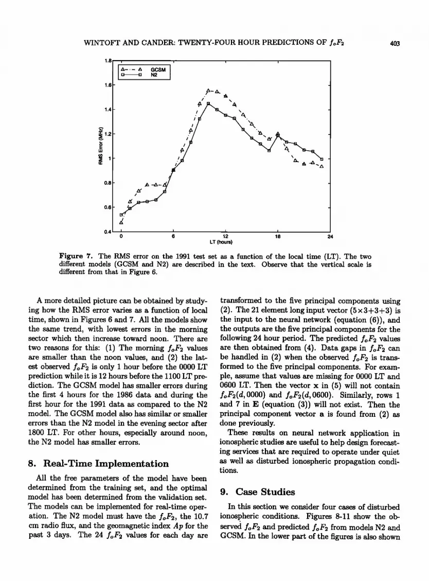
Figure 7. The RMS error on the 1991 test set as a function of the local time (LT). The two different models (GCSM and N2) are described in the text. Observe that the vertical scale is different from that in Figure 6.

A more detailed picture can be obtained by studying how the RMS error varies as a function of local time, shown in Figures 6 and 7. All the models show the same trend, with lowest errors in the morning sector which then increase toward noon. There are

two reasons for this: (1) The morning foF2 values are smaIler than the noon values, and (2) the latest observed foF2 is only I hour before the 0000 LT prediction while it is 12 hours before the 1100 LT prediction. The GCSM model has smaller errors during the first 4 hours for the 1986 data and during the first hour for the 1991 data as compared to the N2 model. The GCSM model also has similar or smaller

errors than the N2 model in the evening sector after 1800 LT. For other hours, especially around noon, the N2 model has smaller errors.

8. Real-Time Implementation

All the free parameters of the model have been determined from the training set, and the optimal model has been determined from the validation set.

The models can be implemented for real-time operation. The N2 model must have the foF2, the 10.7 cm radio flux, and the geomagnetic index Ap for the past 3 days. The 24 foF2 values for each day are

transformed to the five principal components using (2). The 21 element long input vector (5 x 3 + 3 + 3) is the input to the neural network (equation (6)), and the outputs are the five principal components for the following 24 hour period. The predicted foF2 values are then obtained from (4). Data gaps in foF• can be handled in (2) when the observed foF2 is transformed to the five principal components. For example, assume that values are missing for 0000 LT and 0600 LT. Then the vector x in (5) will not contain foF2(d, 0000) and foF2(d, 0600). Similarly, rows 1 and 7 in E (equation (3)) will not exist. Then the principal component vector a is found from (2) as done previously.

These results on neural network application in ionospheric studies are useful to help design forecasting services that are required to operate under quiet as well as disturbed ionospheric propagation conditions.

9. Case Studies

In this section we consider four cases of disturbed

ionospheric conditions. Figures 8-11 show the observed foF2 and predicted foF2 from models N2 and GCSM. In the lower part of the figures is also shown


7

6

-o 4

3 !

2

1

I i i

_ _

I I I I

1 2 3 4 5

5O

4O

3O

2O

0 I I I I 1 2 3 4 5 6

Days in May 1986

Figure 8. (top) Observed foF2 (thick line) and predicted foF2 (N2, thin line; GCSM, dashed line) for a 5 day period in May 1986. (bottom) Ap for the same period.

6

"5 _o

4

3

/

1 14 15 16

35

3O

25

2O

15

10

5

0

! i

/

Days in October 1986

Figure 9. (top) Observed foF2 (thick line) and predicted foF2 (N2, thin line; GCSM, dashed line) for a 5 day period in October 1986. (bottom) Ap for the, same period.

WINTOFT AND CANDER: TWENTY-FOUR HOUR PREDICTIONS OF loft. 405

14

12

10

2 23

2OO

150

100

23 24

Days in March 1991

Figure 10. (top) Observed loft. (thick line) and predicted loft. (N2, thin line; GCSM, dashed line) for a 5 day period in March 1991. (bottom) Ap for the same period.

9

8

7

6

5

4

3

4 5 6 7 8

I I I I

.

/ / \/

-

2OO

150

100

0 I I I I 4 5 6 7 8 9

Days in June 1991

Figure 11. (top) Observed loft. (thick line) and predicted loft. (N2, thin line; GCSM, dashed line) for a 5 day period in June 1991. (bottom) Ap for the same period.


the geomagnetic index Ap. Each case will be dis- cussed in the following.

9.1. May 1986

During 1986, i.e., at solar minimum, there are few large geomagnetic storms. In only 13% of the days, Ap exceeds 20 nT. In the example shown in Figure 8, Ap is around 40 nT over two days. The observed foF2 starts with a positive storm on May 2 and then becomes a negative storm on May 3. For both models (N2 and GCSM) the predicted foF2 follows well the observed foF2 before and after the storm. However, during the storm there are large differences. The GCSM model predicts a negative storm over both days, while the N2 model does not respond at all to the increased Ap.

9.2. October 1986

During October 13 and 14 (Figure 9) Ap is around 30 nT, which does not seem to influence the observed loft. The N2 model follows well the observations as it in this case also does not react to the increased Ap. The GCSM model, however, does respond to Ap and predicts values smaller than the observed values.

9.3. March 1991

During high solar activity in 1991 there are more days with large Ap as compared to 1986; 36% of the days have Ap larger than 20 nT. The period over March 23-28, 1991 (Figure 10), has a large storm over 3 days where Ap is over 100 nT. In this case the N2 model reacts to the increased Ap; however, it does not really reach the low observed loft. Prestorm and poststorm days are well predicted. The prediction from the GCSM model starts with a higher value on March 23, and then it decreases as a consequence of the increased Ap.

9.4. June 1991

The variation of foF2 during the summer (Fig- ure 11) is more irregular than during the winter. Both models fail to predict the ionospheric storm during this event. However, the nighttime values on June 6 are reasonably predicted from the N2 model.

10. Discussion and Conclusions

An ionospheric forecast is a prediction for a specific time and copes with the day-to-day variability in the

ionosphere. To develop ionospheric forecasting, applied research on forecasting must be integrated with advances in ionospheric research. Artificial neural networks are efficient tools for these types of prob- lems as they can cope with nonlinearities and different observed quantities. Furthermore, the classical ionospheric forecasting methods developed up to now depend on successful solar and magnetospheric fore- casts, and limited knowledge of solar-magnetospheric fields limits ionospheric forecasting significantly.

The results presented in sections 7-9 demonstrate the potential of neural networks to predict the ionospheric parameter foF2 24 hours ahead both in quiet and in disturbed conditions. This attempt to develop a model for the prediction of the day-to-day variability of foF2 at the Slough ionospheric station 24 hours ahead, using artificial neural networks is promising. The strength of the neural network model is that new parameters can be included in future work to improve the predictions further.

From the case studies it is seen that the negative ionospheric storm in Figure 10 is delayed by -• 1 day from the magnetospheric storm. This can be examined in more detail by studying the Dst, AE, and Kp indices. On the morning of March 24 there is a huge peak in AE, with Kp > 8, and during the day the activity goes down but is still on a high level (Kp - 5). In the afternoon there is a new burst of activity which peaks in Dst, AE, and Kp at around midnight, and the following day there is a negative ionospheric storm. An explanation of this ionospheric storm evolution is given by Pr51ss [1995]. This is the reason why the neural network is able to predict the negative ionospheric storm based on Ap from the previous day.

However, using a daily index like Ap will lead to the problem that the network will not be able to dis- tinguish between negative and positive ionospheric storms. This is what happens in Figure 8, where there is a positive ionospheric storm on May 2 and a negative storm on May 3. A burst of substorm activity around noon, as seen in AE, leads to the positive ionospheric storm. Then, the magnetospheric activity increases again, a new storm reaches its maximum level of disturbance around midnight, and the following day an ionospheric negative storm develops. The network fails to predict the negative storm probably because there are now two contradicting input pat- terns from May 2 to make the prediction of May 3: (1) a higher than average value in foF• and (2) a moderate storm in ,4p.


The future development of a model to predict foF• 24 hours ahead includes the study of the other principal components (PCs). As was seen from the validation (Figure 3) there is no major improvement in using the nonlinear neural network as compared to the linear filter when the PCs are the only input. Although we used the PCs that describe most of the variance in loft, there might still be important nonlinear information in the other PCs.

Another improvement would be the inclusion of a magnetospheric storm index with a time resolu- tion better than a day, such as hourly AE [Wintort and Cander, 1999b] and hourly Dst, or 3 hour Kp. None of these indices are available in real time al-

though preliminary values exist with a time lag of 6 hours or more. However, all these indices can be successfully predicted in real time using solar wind plasma and magnetic field data [Lundstedt and Wintort, 1994; Gleisner et al., 1996; Wu and Lund- stedt, 1997; Boberg et al., 1999], which of course is critically dependent on the existence a solar wind spacecraft.

Ackn6wledgments. Peter Wintoft is grateful to the Royal Society and to

the Royal Swedish Academy of Sciences for supporting a two month study visit to the Radio Communications Research Unit at the Rutherford Appleton Laboratory. Both authors are grateful to I. Kutiev for providing the ACM and GCSM data. This work has been funded by the Radiocommunications Agency of the DTI as part of the National Radio Propagation Program at Rutherford Appleton Laboratory.

References

Altinay, O., E. Tulunay, and Y. Tulunay, Forecasting of ionospheric critical frequency using neural network, Geophys. Res. Lett. œ•, 1467-1470, 1997.

Boberg, F., P. Wintoft, and H. Lundstedt, Real time Kp predictions from solar wind data using neural networks, Phys. Chem. Earth, in press, 1999.

Cander, L. R. and X. Lamming, Neural networks in ionospheric prediction and short-term forecasting, loth In- ternational Conference on Antennas and Propagation, 1J-17 April 1997, Edinburgh, IEE Conf. Publ., .i36, 2.27-2.30, 1997.

Cander, L. R., M. M. Milosavljevic, S.S. Stankovic, and S. Tomasevic, Ionospheric forecasting technique by ar- tifical neural network, Electron. Lett., 3J(16), 1573- 1574, 1998.

Davies, K., Ionospheric Radio, Peter Peregrinus, London, 1990.

Francis, N.M., A.G. Brown, A. Akram, P.S. Cannon, and D.S. Broomhead, Non-linear prediction of the iono-

spheric parameter foF•., in Proceedings of the Second International Workshop on Artificial Intelligence Ap- plications in Solar-terrestrial Physics, ESA WPP-iJ8 Proc., edited by I. Sandahl and E. Jonsson, pp. 219- 223, Eur. Space Agency, Paris, 1998.

Francis, N.M., A.G. Brown, P.S. Cannon, and D.S. Broomhead, Non-linear interpolation of missing points within the hourly foF2 time series, in Proceedings of the Workshop on Space Weather, ESA WPP-155 Proc., pp. 419-422, Eur. Space Agency, Paris, 1999a.

Francis, N.M., A.G. Brown, P.S. Cannon, A. Akram, and D.S. Broomhead, Novel non-linear techniques for the prediction of noisy geophysical time series that contain a significant proportion of data drop outs, Phys. Chem. Earth, in press, 1999b.

Gleisner, H., H. Lundstedt, and P. Wintoft, Predicting geomagnetic storms from solar-wind data using time- delay neural networks, Ann. Geophys., 1•, 679-686, 1996.

Goodman, J. M., HF Communications: Science and Technology, Van Nostrand Reinhold, New York, 1992.

Haykin, S., Neural Networks: A Comprehensive Founda- tion, Indianapolis, Indiana 1994.

Heckman, G., K. Marubashi, M. A. Shea, D. F. Smart, and R. Thompson (Eds.), Solar- Terrestrial Predic- tions: V, Reg. Warning Cent. Tokyo, Ibaraki, 1997.

Houminer, Z., and H. Soicher, Improved short-term predictions of foF•. using GPS time delay measurements, Radio Sci., 31(5), 1099-1108, 1996.

Johnson, E. E., R.I. Desourdis, G. D. Earle, S.C. Cook, and J. C. Ostergaard, Advanced High-Frequency Radio Communication, Artech House Publishers, Norwood, Mass., 1997.

Jolliffe, I.T., Principal Component Analysis, Springer- Verlag, New York, 1986.

Kumluca, A., E. Tulunay, I. Topalli, and Y. Tulunay, Temporal and spatial forecasting of ionospheric critical frequency using neural networks, Radio Sci., 3J(6), 1497-1506, 1999.

Kutiev, I., P. Muhtarov, L. R. Cander, and M.F. Levy, Short-term prediction of ionospheric parameters based on autocorrelation analysis, Ann. Geofis., •œ, 121-127, 1999.

Lamming, X., and L. R. Cander, Monthly median foF2 modelling COST251 area by neural networks, Phys. Chem. Earth, œ•, 349-354, 1999.

Lundstedt, H., and P. Wintoft, Prediction of geomagnetic storms from solar wind data with the use of neural

networks, Ann. Geophys., 12, 19-24, 1994. McNamara, L. F., The Ionosphere: Communications,

Surveillance, and Direction Finding, Orbit Books, Malabar, Fl., 1991.

Muhtarov, P., and I. Kutiev, Autocorrelation method for temporal interpolation and short-term prediction of ionospheric data, Radio Sci., 3•(2), 459-464, 1999.

Piggott, W. R., and K. Rawer, U.R.S.I. handbook of ionogram interpretation and reduction, Rep. UA G-œ3, Natl. Oceanic and Atmos. Admin., Boulder, Colo., 1972.

Poole, A.W.V., and L.A. McKinnel, Short term predic-

4O8 WlNTOFT AND CANDER: TWENTY-FOUR HOUR PREDICTIONS OF foF2

tion of foF2 using neural networks, in Proceedings of the XXV General Assembly URSI, 1996, Rep. UAG- 105, pp. 109-111, World Data Cent. A for Sol.-Terr. Phys., Boulder, Colo., 1998.

PrSlss, G.W., Ionospheric F-region storms, in Handbook of Atmospheric Electrodynamics, vol. 2, edited by H. Volland, pp. 195-248, CRC Press, Boca Raton, Fl., 1995.

Reinisch, B. W., Ionosonde, in Upper Atmosphere, edited by W. Dieminger, G. K. Hartmann, and R. Leitinger, pp. 370-381, Springer-Verlag, New York, 1996.

Rishbeth, H., F-region storms and thermospheric dynamics, J. Geomagn. Oeoelectr., •3, 513-524, 1991.

Wilkinson, P. J., E. Szuszczewicz, A. Danilov, D. R. Lakshmi, T. Fuller-Rowell, and T. Maruyama, Iono- spheric Working Group report, in Solar-Terrestrial Predictions: V, pp. 12-17, Reg. Warning Cent., Tokyo, Ibaraki, 1997.

Williscroft, L.-A., and A.W.V. Poole, Neural networks, loft, sunspot number and magnetic activity, Geophys. Res. Left., œ3, 3659-3662, 1996.

Wintoft, P., and L. R. Cander, Short-term prediction of foF• using time-delay neural networks, Phys. Chem. Earth, œ•((4), 343-348, 1999a.

Wintoft, P., and L. R. Cander, Ionospheric foF• storm forecasting using neural networks, Phys. Chem. Earth, in press, 1999b.

Wu, J.-G., and H. Lundstedt, Neural network modeling of solar wind-magnetosphere interaction, J. Geophys. Res., 10œ, 14,457-14,466, 1997.

L. R. Cander, CLRC Rutherford Appleton Labora- tory, Chilton, Didcot, Oxon OXll 0QX, England, U.K. ([email protected])

P. Wintoft, Solar-Terrestrial Physics Division, Swedish Institute of Space Physics, Scheelev•igen 17, SE-223 70 Lund, Sweden. ([email protected])

(Received December 23, 1998; revised November 3, 1999; accepted November 8, 1999.)

Documents

Twenty-four hour predictions of f 0 F 2 using time delay neural networks