arX

iv:c

ond-

mat

/050

5314

v2 [

cond

-mat

.mes

-hal

l] 2

3 N

ov 2

005

Two-electron lateral quantum-dot molecules in a magnetic field

M. Helle,∗ A. Harju, and R. M. NieminenLaboratory of Physics, Helsinki University of Technology, P. O. Box 1100 FIN-02015 HUT, Finland

(Dated: February 2, 2008)

Laterally coupled quantum dot molecules are studied using exact diagonalization techniques. Weexamine the two-electron singlet-triplet energy difference as a function of magnetic field strengthand investigate the magnetization and vortex formation of two- and four-minima lateral quantumdot molecules. Special attention is paid to the analysis of how the distorted symmetry affects theproperties of quantum-dot molecules.

PACS numbers: 73.21.La,73.22.-f,75.75.+a,73.21.-b

I. INTRODUCTION

The crossover from two-dimensional electron systems(2DES) to meso- and nanoscale quantum dots (QDs) isan interesting subject. In the infinite quantum Hall sys-tems the actual arrangement of impurities or disorderdoes not play a role, even if the presence of disorder-induced localized states is vital for the Hall plateaus tooccur.1 In the few-electron QDs, the type of disorder iscertainly an important issue. In the past, the majority ofstudies have concentrated on highly symmetric parabolicQDs without disorder. The rich spectrum of crossingenergy levels as a function of magnetic field and stronginteraction effects are nowadays rather well character-ized for the cases with a symmetric confinement poten-tial.2 Recently, the focus has turned to understandingproperties of QDs in less symmetric confinement poten-tials. For example, the rather simple far-infrared excita-tion spectrum of a purely parabolic QD is nowadays wellunderstood,3 whereas the lowered symmetry introducesnew features in the spectrum whose interpretation is notstraightforward at all.4,5,6,7,8,9,10,11 Moreover, the low-ered symmetry also gives rise to modified ground stateproperties such as level anticrossings and altered spin-phase diagram as a function of magnetic field.12,13

After Loss and DiVincenzo proposition,14 coupledquantum dots have gained interest due to possible re-alization as spin-qubit based quantum gates in quantumcomputing.15,16,17 In addition to coherent single-spin op-erations, the two-spin operations are sufficient for assem-bling any quantum computation. Recent experimentshave shown a remarkable success in characterizing thefew-electron eigenlevels,18,19,20 approximating relaxationand time-averaged coherence times and mechanisms,21,22

and reading single-spin or two-spin states23,24 of the QDswhereas the coherent manipulation of spin systems re-mained out of reach until very recent measurements ontwo-spin rotations.25

In this paper we concentrate on two-electron quan-tum dot molecules. These molecules consist of laterally,closely coupled quantum dots. We treat correlation ef-fects between the electrons properly by directly diago-nalizing the Hamiltonian matrix in the many-body ba-sis (exact diagonalization technique). This allows direct

access to the ground state energy levels and all excitedstates for both spin-singlet and spin-triplet states. Westudy these levels as well as singlet-triplet splitting andmagnetizations as a function of magnetic field and dot-dot separation. We also analyze the properties of many-body wave functions in detail.

The magnetic field dependence of the ground state en-ergy and singlet-triplet splitting in non-parabolic QDshave attracted recent interest.12,13,18,26,27,28,29,30,31,32,33

Magnetizations in QDs have been measured indirectlywith transport measurements34 and recently with a di-rect technique with improved sensitivity.35 For both mea-surements, semi-classical approaches cannot explain theresults. Also the magnetizations of nanoscale QDs do notshow non-equilibrium currents and de Haas-van Alphenoscillations which are observed in 2DES and mesoscopicQDs.36 In the nanoscale QDs the quantum confine-ment and Coulomb interactions modify the system com-pared to the 2DES.35 Theoretically, magnetization (atzero temperature) is straightforward to calculate as thederivative of the total energy with respect to magneticfield. Magnetizations have been calculated for a smallnumber of electrons in a parabolic QD,37 in a squaredot with a repulsive impurity,38 as well as for anisotropicQDs,27 and for self-assembled QDs and quantum rings.39

The magnetization curves have been calculated usingdensity-functional theory for rectangular QDs26 and us-ing the Hartree approximation for other types of non-circular QDs.40 A tight-binding model for 10-100 elec-trons in a single or two coupled QDs has been used tocalculate magnetization curves.41

Calculations of vortices in QDs have also attractedmuch interest lately.42,43,44,45,46 Even if the vortices arenot directly experimentally observable, they reveal in-teresting properties of electron-electron correlations andof the structure of the wave function. The nucleationof vortices in QD systems could perhaps be observed bymeasuring magnetizations, where each peak would corre-spond to one vortex added in the system. However, themagnetization is difficult to measure for a small numberof electrons, especially with direct methods. Moreover,in a non-circular symmetry, as in quantum dot molecules,and at high magnetic field strengths the magnetizationcurves may become more complicated.

In our previous studies we have examined the proper-

2

ties of two-electron, two-minima quantum-dot molecules(QDM) in a magnetic field. The ground state as afunction of magnetic field was found to have a highlynon-trivial spin-phase diagram and a composite-particlestructure of the wave function.12 Also the calculatedfar-infrared absorption spectra in two-minima QDMsrevealed clear deviations from the Kohn modes of aparabolic QD. Surprisingly, the interactions of the elec-trons smoothened the deviations instead of enhancingthem.5 In Ref. 47 we briefly discuss some of the resultsof square-symmetric four-minima QDM.

In this paper, we study in detail the properties of dif-ferent QDMs. Three different QDM confinements arestudied thoroughly and their properties are comparedto parabolic-confinement single QDs. First, we calcu-late measurable quantities such as energy eigenstates,singlet-triplet splittings and magnetizations as a func-tion of magnetic field. Secondly, non-measurable quan-tities, such as conditional densities, vortices, total densi-ties, and the most probable positions are used to analyzethe nature of the interacting electrons in quantum statesand also to analyze and understand the properties of themeasurable quantities. This paper is an extension toour previous calculations of QDMs.12,47 We study a two-minima QDM (double dot), a square-symmetric four-minima QDM and a rectangular-symmetric four-minimaQDM. The aim of this paper is to study how the con-finement potential affects the properties of interactingelectrons in a low-symmetry QD.

This paper is organized as follows: In Section II we ex-plain how the quantum-dot molecules are modeled andwhat kind of basis we use in the exact diagonalizationmethod. We also discuss calculation of magnetizationsand the conditional single-particle wave function whichwe use to locate the vortices and study the conditionaldensity. In the following four sections we present ourresults. In Section III we discuss properties of a sin-gle parabolic quantum dot, and in Sec. IV we analyzethe properties of a double dot. In Sec. V we present re-sults for the square-symmetric four-minima quantum-dotmolecule, and finally in Sec. VI the results for rectangu-lar four-minima quantum-dot molecule. The analysis ofthe results is presented in Section VII. The summary isgiven in Section VIII.

II. MODEL AND METHOD

We model the two-electron QDM with the two-dimensional Hamiltonian

H =

2∑

i=1

(

(−i~∇i − ecA)2

2m∗+ Vc(ri)

)

+e2

ǫr12, (1)

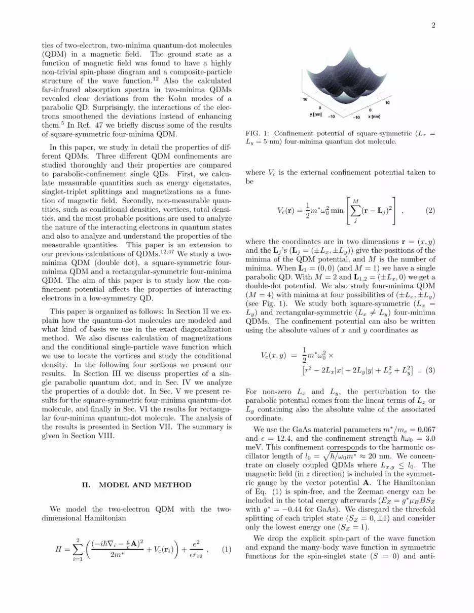
FIG. 1: Confinement potential of square-symmetric (Lx =Ly = 5 nm) four-minima quantum dot molecule.

where Vc is the external confinement potential taken tobe

Vc(r) =1

2m∗ω2

0 min

M∑

j

(r − Lj)2

, (2)

where the coordinates are in two dimensions r = (x, y)and the Lj ’s (Lj = (±Lx,±Ly)) give the positions of theminima of the QDM potential, and M is the number ofminima. When L1 = (0, 0) (and M = 1) we have a singleparabolic QD. With M = 2 and L1,2 = (±Lx, 0) we get adouble-dot potential. We also study four-minima QDM(M = 4) with minima at four possibilities of (±Lx,±Ly)(see Fig. 1). We study both square-symmetric (Lx =Ly) and rectangular-symmetric (Lx 6= Ly) four-minimaQDMs. The confinement potential can also be writtenusing the absolute values of x and y coordinates as

Vc(x, y) =1

2m∗ω2

0 ×[

r2 − 2Lx|x| − 2Ly|y| + L2x + L2

y

]

. (3)

For non-zero Lx and Ly, the perturbation to theparabolic potential comes from the linear terms of Lx orLy containing also the absolute value of the associatedcoordinate.

We use the GaAs material parameters m∗/me = 0.067and ǫ = 12.4, and the confinement strength ~ω0 = 3.0meV. This confinement corresponds to the harmonic os-cillator length of l0 =

√

~/ω0m∗ ≈ 20 nm. We concen-trate on closely coupled QDMs where Lx,y ≤ l0. Themagnetic field (in z direction) is included in the symmet-ric gauge by the vector potential A. The Hamiltonianof Eq. (1) is spin-free, and the Zeeman energy can beincluded in the total energy afterwards (EZ = g∗µBBSZ

with g∗ = −0.44 for GaAs). We disregard the threefoldsplitting of each triplet state (SZ = 0,±1) and consideronly the lowest energy one (SZ = 1).

We drop the explicit spin-part of the wave functionand expand the many-body wave function in symmetricfunctions for the spin-singlet state (S = 0) and anti-

3

3 4 5 6 7 80

0.2

0.4

0.6

0.8

1

Ene

rgy

erro

r [%

]

Basis size

m=0m=1m=2m=3

FIG. 2: Relative error in the energy of parabolic two-electronQD at B = 0 as a function of the basis size nx = ny from 3to 8, which corresponds to around 40-2000 many-body basisfunctions in the expansion. The relative angular momentumstate of electrons is denoted with m.

symmetric functions for the spin-triplet state (S = 1).

ΨS(r1, r2) =∑

i≤j

αi,j{φi(r1)φj(r2)

+(−1)Sφi(r2)φj(r1)}, (4)

where αi,j ’s are complex coefficients. The one-body basisfunctions φi(r) are 2D Gaussians.

φnx,ny(r) = xnxynye−r2/2, (5)

where nx and ny are positive integers. The complex co-efficient vector αl and the corresponding energy El arefound from the generalized eigenvalue problem where theoverlap and Hamiltonian matrix elements are calculatedanalytically. The matrix is diagonalized numerically.

The basis is suitable for closely coupled QDs. At largedistances and at high magnetic field we expect less accu-rate results. The accuracy may also depend on the sym-metry of the state. At zero magnetic field the parabolic

two-electron QD can be modeled with a very good pre-cision by expanding the basis (in a given symmetry) inrelative coordinates. In Fig. 2 we compare the energyof the very accurate solution and the one using our basis(for a parabolic QD) as a function of the basis size, wherethe maximum nx = ny ranges from 3 to 8. These valuescorrespond to around 40 − 2000 many-body configura-tions in the expansion. States with m = 0, 1, 2, 3 refer todifferent relative angular momentum states. The relativeerror, even with the smallest basis studied nx = ny = 3,is less than one percent and decreases rapidly with theincreasing basis size. The greatest error is found for them = 0 state.

The magnetization can be calculated as the derivativeof the total energy with respect to magnetic field. It canbe divided into to parts, paramagnetic and diamagnetic,

M = −∂E∂B

= 〈Ψ| e

2m∗cLz + g∗µBSz |Ψ〉

− e2

8m∗c2〈Ψ|

∑

i

r2i |Ψ〉B, (6)

−50 −25 0 25 500

0.2

0.4

0.6

0.8

1

x [nm]

B = 1 T

(a) one e−

S=0S=1

−50 −25 0 25 500

0.2

0.4

0.6

0.8

1

x [nm]

B = 8 T

(b) one e−

S=0S=1

−50 −25 0 25 500

0.2

0.4

0.6

0.8

1

x [nm]

B = 1 T

(c) one e−

S=0S=1

−50 −25 0 25 500

0.2

0.4

0.6

0.8

1

x [nm]

B = 8 T

(d) one e−

S=0S=1

FIG. 3: One-body density (dotted line), two-body spin-singlet state (dashed line) and two-body spin-triplet state(solid line) along x axis. One of the electrons is fixed atthe most probable position in the x axis (x∗) and the condi-tional density is plotted for the other electron (|ψc(r)|

2 =|ΨS[(x, y), (x∗, 0)]|2/|ΨS [(−x∗, 0), (x∗, 0)]|2). The peaks onthe left-hand side also indicates the most probable position,therefore by reflecting the peak position to the right-hand sideof the x axis one can perceive the position of the fixed elec-tron. (a) and (b) show the densities of parabolic QD at twodifferent magnetic field values (B = 1 and 8 T), (c) and (d)represent two-minima QDM with Lx = 20 nm. The confine-ment potential, Vc, is plotted with gray color on each figure.

where the former is constant as a function of magneticfield, for a given angular momentum and spin state, andthe latter depends linearly on magnetic field. The dia-magnetic contribution to the magnetization is also a mea-sure of the spatial extension of the ground state.38

Total electron density can be obtained by integratingone variable out from the two-body wave function

n(r1) =

∫

dr2|ΨS(r1, r2)|2. (7)

In practice we do not perform numerical integration. Thedensity is directly calculated in our diagonalization codewhere the required matrix elements are calculated ana-lytically.

We analyze the two-body wave function by construct-ing a conditional single-particle wave function

ψc(r) = |ψc(r)|eiθc(r) =ΨS [(x, y), (x∗2, y

∗2)]

ΨS [(x∗1, y∗1), (x∗2, y

∗2)], (8)

where one electron is fixed at position (x∗2, y∗2) and the

density (|ψc(r)|2) and phase (θc(r)) of the other electroncan be studied. One of the electrons is usually fixed atthe most probable position (x∗2, y

∗2), but we also analyze

ψc(r) when the other electron is fixed at some other po-sition. The most probable positions of electrons (r∗1, r

∗2)

are found by maximizing the absolute value of the wavefunction with respect to coordinates r1 and r2:

maxr1,r2

|ΨS(r1, r2)|2 → r∗1, r

∗2. (9)

4

One should note that |ψc(r)|2 is not normalized to onewhen integrated over the two-dimensional space becauseit describes the electron at position (x, y) on the con-dition that the other electron is fixed at (x∗2, y

∗2). In-

stead, |ψc(r)|2 is normalized so that it equals to onewhen x = x∗1, y = y∗1 . Using the conditional single-particle wave function we can study the conditional den-sity |ψc(r)|2 and the phase θc(r).

To illustrate how the properties of the many-body wavefunction can be examined with the conditional single-particle wave function, we compare interacting two-bodyconditional densities to non-interacting two-body densi-ties in Fig. 3. The non-interacting two-body density isthe same as the single-particle density (up to a normal-ization). We call it the one-body density hereafter. Weplot the one-body, two-electron singlet (S = 0) and two-electron triplet (S = 1) conditional single-particle densi-ties along x-axis. The other electron, in the two-electronsystems, is fixed at the most probable position (x∗) onthe right-hand side of the x-axis.

Fig. 3 (a) and (b) show conditional densities of thesingle parabolic QD at B = 1 and 8 T magnetic fields.The one-body density is located at the center since nocorrelation effects push it towards the edges of the dot.The peak of the triplet state is found further at the edgeof the dot than the singlet peak since Pauli exclusionprinciple ensures that the electrons of the same spin arepushed further apart than the electrons with the oppositespins. Notice that the conditional density of the tripletstate goes to zero where the other electron is fixed, justbefore x = 20 nm, whereas in the singlet state there is afinite probability to find the electron around the point ofthe fixed electron.

Fig. 3 (c) and (d) show the same data for Lx = 20 nmtwo-minima QDM. In high magnetic fields and at largedot-dot separations the difference between singlet andtriplet densities reduces. In QDMs, with a sufficientlylarge distance between the dots and in high magnetic fieldalso the one-body density localizes into the individualdots (see Fig. 3 (d)).

III. PARABOLIC TWO-ELECTRON QUANTUMDOT (L = 0)

We start our analysis from the single parabolic quan-tum dot. The two-electron parabolic QD is studied ex-tensively in the literature but presenting results hereserves as a good starting point for understanding prop-erties of quantum dot molecules.

A. Energy levels

Energy levels of the parabolic QD are plotted in Fig. 4as a function of magnetic field. Fig. 4 (a) shows non-interacting two-body energy levels, (b) the ten lowestlevels for two-body spin-singlet states (S = 0), and (c)

for two-body spin-triplet (S = 1) states. In (d) threelowest singlet and triplet levels are shown in the sameplot. The non-interacting spectrum is obtained by oc-cupying two electrons in the Fock-Darwin energy lev-els. The first eigenvalue at zero field equals two times(Ne = 2) the confinement potential (~ω0 = 3 meV,E1(B = 0) = 3 + 3 = 6 meV) and the second level repre-sents one electron in the lowest Fock-Darwin level and theother electron in the next one (E2(B = 0) = 3 + 6 = 9meV). Many non-interacting energy levels are degener-ate, also as a function of magnetic field. (In a less sym-metric confinement, the degeneracies are lifted). Due todegeneracies, only six levels are seen in Fig. 4 (a). If theinteractions are included, the spectra become much morecomplicated and many more level crossings are observed.One can also see how the energy scale is modified. Inthe spin-singlet spectra the ground state energy is almostdoubled if the Coulomb interaction is included.

To see the crossing singlet and triplet states moreclearly, we plot the three lowest energy levels of spin sin-glet (dashed line) and spin triplet (solid line) in Fig. 4 (d)up to B = 6 T. In a weak magnetic field the ground stateof the two-electron QD is spin-singlet (S = 0), whichchanges to spin-triplet (S = 1) as the magnetic field in-creases and then again to singlet and finally to triplet (atB ≈ 6.3 T, not visible in Fig. 4 (d)).

B. Singlet-triplet splitting and magnetization

In Fig. 5 (a) we plot the energy difference of the lowesttriplet and singlet states up to B = 8 T. Altering singletand triplet states are also seen in higher magnetic fieldswith a decreasing energy difference between the states.However, if one includes the Zeeman term, the tripletstate is favored over the singlet state at highB. Thereforethe system becomes spin polarized.

The transitions between the states can also be exam-ined from the magnetization curves plotted in Fig. 5 (b).The non-interacting magnetization is a smooth curve asno crossings are present in the lowest energy level. Theorbital angular momentum in the non-interacting two-electron ground state does not change, and thus onlythe diamagnetic effects are seen in the magnetization.The non-interacting electrons have a smaller spatial ex-tent of the wave function compared to the interactingelectrons. Therefore, at low fields, when the response ispurely diamagnetic, the magnetization curve of interact-ing electrons has a lower absolute value in Fig. 5 (b).The magnetization curve of interacting electrons showsabrupt increase of the otherwise smooth curve whenevertwo levels cross (see also Fig. 4 (d)). The peaks in mag-netization are solely due to interactions.

5

FIG. 4: Ten lowest energy levels of parabolic QD (Lx = 0, Ly = 0) as a function of magnetic field of (a) non-interactingtwo-body, (b) two-body singlet state (S = 0) and (c) two-body triplet state (S = 1). Some of the states in (a) are degenerate.(d) three lowest energy levels of singlet (dashed line) and triplet (solid line) as a function of magnetic field up to B = 6 T forparabolic QD (Lx = Ly = 0). In (b) the first singlet ground state corresponds to angular momentum m = 0 which changes tom = 2 at B ≈ 2.7 T. In (c) the first triplet ground state is m = 1 and it changes to m = 3 at B ≈ 5.8 T. In (d) the first groundstate equals to m = 0 singlet, then ground state is m = 1 triplet followed by m = 2 singlet and m = 3 triplet, where the latteris not visible as a ground state in (d). Zeeman energy is included in the triplet energies (EZ = −2 × 12.7B[T ] µeV in GaAs).

FIG. 5: Triplet-singlet energy difference in (a) and magnetiza-tion in (b) for parabolic QD (Lx = Ly = 0). The lower curvein (a) shows the singlet-triplet splitting with Zeeman energyincluded. The smooth curve in (b) represents the magneti-zation of two non-interacting electrons and the other curveshows the magnetization for two interacting electrons. Atlow magnetic field values, the ground state is the angular mo-mentum m = 0 singlet, which shows as positive values in thetriplet-singlet energy difference of (a) and as a smooth curvein (b). When the first transition from m = 0 singlet to m = 1triplet occurs triplet-singlet energy difference changes its signfrom positive to negative and there appears a peak in magne-tization. Change of m = 1 triplet to m = 2 singlet and fromm = 2 singlet to m = 3 triplet appear in the same way aspeaks in magnetization and changes of sign in triplet-singletsplitting. Magnetization is given in the units of effective Bohrmagnetons µ∗

B = e~/2m∗ (µ∗B = 0.87 meV/T for GaAs).

C. Wave function analysis & vortices

We will now analyze the two-body wave functions andstudy in more detail singlet-triplet transitions in the sin-gle QD. The first singlet-triplet transition can be beunderstood with the simple occupation of the lowestsingle-particle states: In the singlet state the two elec-trons occupy the lowest energy eigenstate with oppositespins (S = 0). As the magnetic field increases, the en-ergy difference between the lowest and the second low-

est single-particle levels decreases. (See non-interactingenergy levels in Fig. 4 (a)). At some point the ex-change energy in the spin-triplet state becomes largerthan the energy difference between the adjacent energylevels. Thus, the singlet-triplet transition occurs and theadjacent eigenlevels are occupied with electrons of paral-lel spins (S = 1).

However, the true solution of the two-electron QDMis much more complicated than the occupation of single-particle levels and inclusion of exchange energies. Inter-action between the electrons changes the situation dras-tically. This can already be seen by comparing the single-particle energy levels of Fig. 4 (a) to singlet and tripletenergy levels in (b) and (c). As a signature of complexmany-body features, many singlet-triplet transitions areseen as a function of B. There are two trends competingin the ground state of a quantum dot when the magneticfield increases. The magnetic field squeezes the electrondensity towards the center of the dot and the Coulombrepulsion of electrons increases at the same time as theelectron density is forced to a smaller volume. At somepoint it is favorable to change to a higher angular momen-tum ground state, which pushes electron density furtherapart and reduces the Coulomb energy. Therefore as afunction of the magnetic field a series of different angularmomentum states are seen.

The altering singlet and triplet states can also be un-derstood in terms of composite particles of electrons andattached flux quanta.49 The starting point for under-standing the ground state changes and flux quanta is toconsider the two-electron parabolic QD (as discussed inthis Section), which has an exact solution for the wavefunction of the form

Ψ = (x12 + iy12)mf(r12)e

−(r2

1+r2

2)/2, (10)

where x12 = x1−x2, y12 = y1−y2 and r12 = |r1−r2| arethe relative coordinates of the two electrons,m is the rela-

6

FIG. 6: (a)-(e) contours of conditional density |ψc(x, y)|2 and

phase of the conditional wavefunction θc(x, y) in gray-scalefor parabolic QD (Lx = Ly = 0). (White equals θc = 0 anddarkest gray θc = 2π). Magnetic field value and the spin typeare plotted on top of each figure. The plus sign (+) indicatesthe position of the fixed electron and small circles indicatethe positions of the vortices. In (f) contours of total electrondensity of the three-vortex triplet state are plotted in thebackground and positions of the vortices are solved when thefixed electron is in three different positions. Fixed electron ismarked with the plus sign and vortices with circles. The mostprobable position is marked with a star, on the left-hand sidefor clarity.

tive angular momentum and f is a correlation factor.12,50

The zeros of the wave function (vortices in relative coor-dinates) are placed on z12 = x12+iy12 = 0 with a windingnumber given by the relative angular momentum m. Inthe first S = 0 state the relative angular momentum ofelectrons is zero (m = 0). When the magnetic field in-creases the ground state changes to spin triplet S = 1,where the relative angular momentum of electrons equalsone (m = 1) and in the second singlet state m = 2, andso on.With increasing magnetic field the relative angularmomentum of electrons increases and altering singlet andtriplet states are seen (if the Zeeman term is excluded).The transitions occur because in the states with largem the Coulomb repulsion becomes smaller at the cost ofhigher confinement and kinetic energies. As the increas-ing magnetic field squeezes electrons to a smaller area, itis favorable to move to largerm to minimize the total en-ergy. One should note that with even m the spatial partof the total wave function is symmetric and therefore thespin part should be antisymmetric (S = 0). With odd mthe spin part is symmetric (S = 1).

When the angular momentum increases, the increasedrotation induces vortices in the system. As we have amany-body system, the rotation is a correlated motion ofelectrons and can be studied in the relative coordinatesof electrons. Vortices can be found by locating the zerosof the wave function and studying the phase of the wavefunction when going around each of the zeros. As thevortices are seen in the relative coordinates, and are not

visible in the density, we examine the conditional single-particle wave function ψc(r) (of Eq. (8)), where one elec-tron is fixed in the most probable position (on the x axis,the system is circular symmetric). The vortices are seenin the zeros of ψc. When the phase part, θc, is integratedaround a closed path encircling the zero, we obtain thewinding number of the vortex (

∮

θc(r)dr = m2π).

In a parabolic two-electron QD vortices are automati-cally attached on top of the electrons, where the relativeangular momentum m equals the winding number of avortex. In a less symmetric potential the center of massand relative variables do not decouple and one would ex-pect more complicated structures as can be seen in latersections. The simple form of the wave function in Eq.(10) is due to separation of the center of mass and rela-tive coordinates in the parabolic confinement.

Calculated vortices and conditional densities of the sin-gle QD are shown in Fig. 6. The contours show the con-ditional electron density, |ψc|2, and the gray-scale back-ground marks the phase of the conditional wave func-tion, θc, where the white color equals θc = 0 and thedarkest gray θc = 2π. The positions of the vortices aremarked with circles (o), and the other electron is fixed atthe most probable position (r∗2) shown with a plus sign(+).The lines of dark gray and white borders correspondto a sudden phase change of 2π if the line is crossed. Thenumber of flux quanta attached to the electron (or thewinding number of a vortex) can be determined by go-ing around the fixed electron position and calculating thetotal phase change (or counting the lines crossed in thefigure).

In Fig. 6 (a) the phase is constant (no vortices andno relative angular momentum) and the the probabilitydensity of the other electron is located on the left sidebecause of the Coulomb repulsion. In (b) we find onevortex as one border of white and gray is crossed whenthe fixed electron is encircled. In (c) we find two vortices,in (d) three vortices and in (e) four vortices. Fig. 6 (a)corresponds to the first singlet with relative angular mo-mentum m = 0, (b) shows the first triplet with m = 1,(c) the second singlet with m = 2 and (d) the secondtriplet with m = 3. Fig.6 (e) would be the third singletstate but this is not a ground state if the Zeeman termis included. The conditional density shows how the elec-tron localizes to a smaller area when the magnetic fieldincreases. We also notice the enhancement of interac-tion at high B where the density contours are contractedcompared to the low-field conditional densities.

The conditional density and phase are much more sen-sitive to the basis size than e.g. energy eigenvalues. Ina parabolic QD the vortices should appear exactly ontop of the fixed electron. However, in the two-, three-and four-vortex plots, in Fig. 6, the vortices are slightlydisplaced from the fixed electron position. The finite ba-sis expansion does not result in exactly correct vortexpicture. On the other hand, the problem is not very se-rious because the error in energy is not large and vortexpositions are not experimentally observable and we also

7

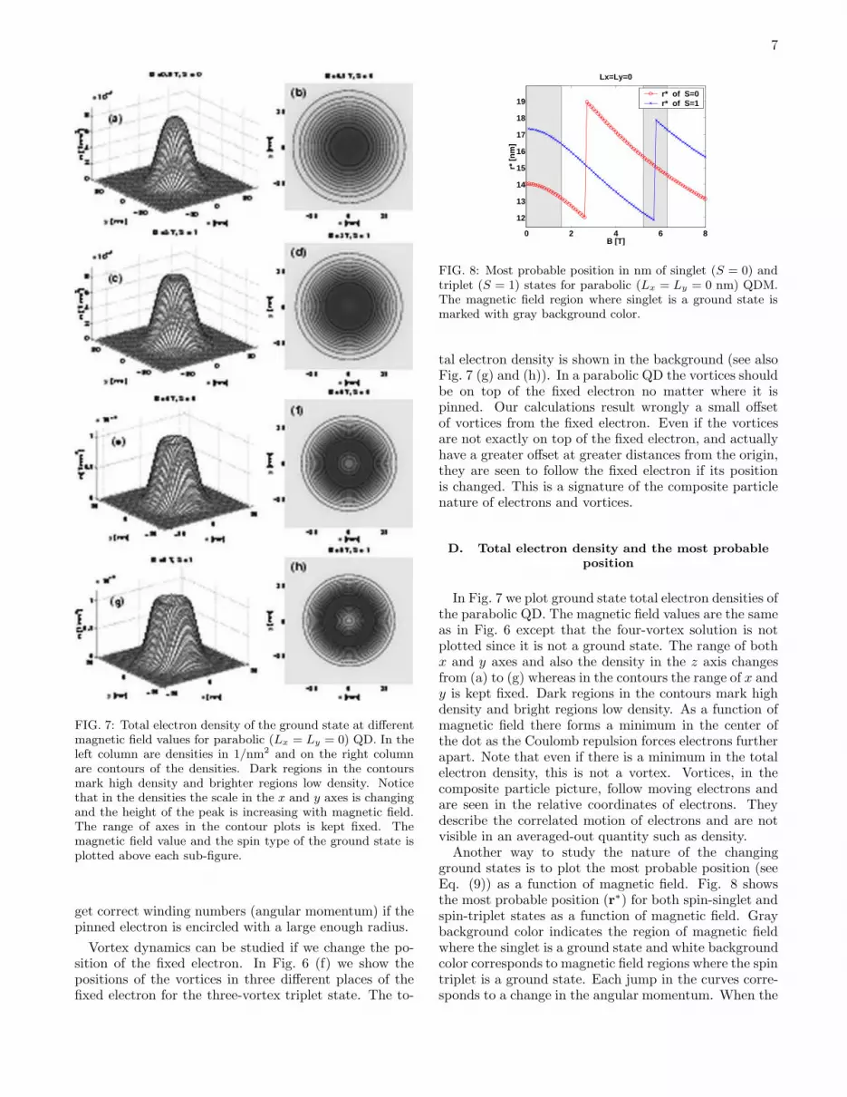
FIG. 7: Total electron density of the ground state at differentmagnetic field values for parabolic (Lx = Ly = 0) QD. In theleft column are densities in 1/nm2 and on the right columnare contours of the densities. Dark regions in the contoursmark high density and brighter regions low density. Noticethat in the densities the scale in the x and y axes is changingand the height of the peak is increasing with magnetic field.The range of axes in the contour plots is kept fixed. Themagnetic field value and the spin type of the ground state isplotted above each sub-figure.

get correct winding numbers (angular momentum) if thepinned electron is encircled with a large enough radius.

Vortex dynamics can be studied if we change the po-sition of the fixed electron. In Fig. 6 (f) we show thepositions of the vortices in three different places of thefixed electron for the three-vortex triplet state. The to-

0 2 4 6 8

12

13

14

15

16

17

18

19

B [T]

r* [n

m]

Lx=Ly=0

r* of S=0r* of S=1

FIG. 8: Most probable position in nm of singlet (S = 0) andtriplet (S = 1) states for parabolic (Lx = Ly = 0 nm) QDM.The magnetic field region where singlet is a ground state ismarked with gray background color.

tal electron density is shown in the background (see alsoFig. 7 (g) and (h)). In a parabolic QD the vortices shouldbe on top of the fixed electron no matter where it ispinned. Our calculations result wrongly a small offsetof vortices from the fixed electron. Even if the vorticesare not exactly on top of the fixed electron, and actuallyhave a greater offset at greater distances from the origin,they are seen to follow the fixed electron if its positionis changed. This is a signature of the composite particlenature of electrons and vortices.

D. Total electron density and the most probableposition

In Fig. 7 we plot ground state total electron densities ofthe parabolic QD. The magnetic field values are the sameas in Fig. 6 except that the four-vortex solution is notplotted since it is not a ground state. The range of bothx and y axes and also the density in the z axis changesfrom (a) to (g) whereas in the contours the range of x andy is kept fixed. Dark regions in the contours mark highdensity and bright regions low density. As a function ofmagnetic field there forms a minimum in the center ofthe dot as the Coulomb repulsion forces electrons furtherapart. Note that even if there is a minimum in the totalelectron density, this is not a vortex. Vortices, in thecomposite particle picture, follow moving electrons andare seen in the relative coordinates of electrons. Theydescribe the correlated motion of electrons and are notvisible in an averaged-out quantity such as density.

Another way to study the nature of the changingground states is to plot the most probable position (seeEq. (9)) as a function of magnetic field. Fig. 8 showsthe most probable position (r∗) for both spin-singlet andspin-triplet states as a function of magnetic field. Graybackground color indicates the region of magnetic fieldwhere the singlet is a ground state and white backgroundcolor corresponds to magnetic field regions where the spintriplet is a ground state. Each jump in the curves corre-sponds to a change in the angular momentum. When the

8

FIG. 9: Triplet-singlet energy difference (∆E = E↑↑ − E↑↓)as a function of magnetic field in two-minima quantum dotmolecule. The energy difference is plotted as a function ofdot-dot separation and magnetic field in (a) without Zeemanenergy and in (c) with the Zeeman energy included (∆E =E↑↑ + EZ −E↑↓). In (b) and (d) the ground state regions ofthe singlet and triplet states are plotted as function of B andL, without and with Zeeman energy, respectively.

singlet changes from m = 0 to m = 2 state at B ≈ 2.7T the most probable position jumps to a higher valueas well. See also energy level crossings in Fig. 4 (b).The outward relaxation, due to the increase of angularmomentum, can be also seen in the density. Similar de-pendence is seen for the triplet state. First the mostprobable position decreases due to contracting electrondensity and then, at some point, it is favorable to moveto a higher angular momentum state which relaxes theelectron density outwards. In higher magnetic field wewould see a sequence of transitions between increasingangular momentum states.

IV. TWO-MINIMA QUANTUM DOTMOLECULE (Lx 6= 0)

A. Singlet-triplet splitting as a function of L

In this section we study two laterally coupled quantumdots. In a two-minima QDM, or double dot, we study thechanges in the ground state spectrum when two QDs, ontop of each other, are pulled apart laterally. In Fig. 9(a) the energy difference of the lowest triplet and singletstates is plotted as a function of the inter-dot spacingand magnetic field. At L = 0 we have a single parabolicQD and the curve coincides with Fig 5 (a). When L 6= 0we have a double dot. Let us now examine some generaltrends of the triplet-singlet energy difference as a functionof dot-dot separation. At small magnetic field the groundstate is a spin singlet, then triplet, and again singlet as

in the single QD, but the transition points change andthe energy differences are smaller at greater distancesbetween the dots than in the single QD. The transitionpoints and regions of singlet and triplet states are plottedin Fig 9 (b). We can also note that all transition pointsare shifted to lower B at large distances between thedots. If the Zeeman energy, that lowers the triplet energy,is included in the total energy the second singlet statedisappears at greater L as can be seen in Fig. 9 (c) and(d). The second singlet is only seen in a small regionwith very closely coupled QDs (L . 2.5 nm). Therefore,subsequent singlet states after the first one are not seenin the double dot if L & 2.5 nm. Similar results areseen in anisotropic QDs where the parabolic confinementof a single QD is elongated continuously to a wire-likeconfinement.27

B. Energy levels of Lx = 5 nm double dot

We choose one distance between the dots, Lx = 5 nm,to study the properties of the double dot in more detail.We plot energy levels, singlet-triplet splitting, magne-tization, vortices, the most probable position and totalelectron density of this double dot in Figs. 10 - 14. Theenergy levels in Fig. 10 are now modified, compared tothe parabolic QD, due to the lower symmetry of the con-finement potential. The circular symmetry is no longerpresent. The lower symmetry shifts and splits degeneratelevels. The non-interacting levels, in Fig. 10 (a), split atzero magnetic field and there is also a small anticrossingof levels, just barely visible in the figure. Also degeneratelevels of the single QD (see Fig. 4 (a)) are now slightlydisplaced in energy, which is mostly seen as thicker linesin Fig. 10 (a). In the interacting spectra, (b) and (c),we see many anticrossings. Also the nature of the lowestlevel does not change abruptly with crossing levels as inthe single QD, but instead we see anticrossing levels. Forexample, there are clear anticrossings in the double dotsinglet states of Fig. 10 (b) whereas states cross in thesinglet state of parabolic QD of Fig. 4 (b).

We plot three lowest singlet and triplet energy levelsin the same figure to see the transition points and energydifferences between the states more clearly (Fig. 10 (d)).The ground state is a singlet at small B, also in the dou-ble dot, and later it changes to triplet. The Zeeman termlowers the triplet energy enough so that no second singlet(ground) state is observed at higher B, even though thesinglet energy becomes very close to the triplet energy atB ≈ 5 T, as can be seen in Fig. 10 (d). The interestinganticrossing of spin singlet between B = 2 and 3 T isnow an excited state as the triplet is the ground state.We also find anticrossing ground state levels in the spintriplet around B ≈ 5.5 T, but the repulsion of levels isnot so clear at high B.

9

FIG. 10: Energy levels of Lx = 5, Ly = 0 two-minima QDM. See Fig. 4 for details.

0 1 2 3 4 5 6 7 8

−0.6

−0.4

−0.2

0

0.2

0.4

0.6

0.8

1

B [T]

∆ E

[meV

]

(a)∆ E = E↑↑ − E↑↓

∆ E = E↑↑ + EZ − E↑↓

0 1 2 3 4 5 6 7 8−2

−1.5

−1

−0.5

0

B [T]

M [

µ B*]

(b)

FIG. 11: Triplet-singlet energy difference (a) and magnetiza-tion (b) for Lx = 5, Ly = 0 two-minima QDM. See Fig. 5 fordetails.

C. Singlet-triplet splitting and magnetization ofLx = 5 nm double dot

The energy difference between the lowest triplet andsinglet states as a function magnetic field in the Lx = 5nm double dot is plotted in Fig. 11 (a), and the magne-tization in Fig. 11 (b). The sharp jump in the magneti-zation corresponds to the singlet-triplet transition. Evenif the system is not circular symmetric, and angular mo-mentum is not a good quantum number, there is an in-crease of the expectation value of angular momentum atthe transition. We can clearly see that the magnetiza-tion increases suddenly at the transition point. AroundB ≈ 5.5 T there is a bump in the magnetization. Thisis exactly at the anticrossing point of the triplet state.Therefore the symmetry of the triplet state changes orthe magnetic moments of the electrons change. This timeit is not seen as an abrupt change but as a continuousone. Similar magnetization curves are seen in asymmet-ric QDs with a correct deformation from the parabolicconfinement to a more wire-like confinement.27

D. Vortices of Lx = 5 nm double dot

In the case of QDMs the states cannot be identifiedwith angular momentum since it is not a good quantumnumber. However, we can still study vortices and condi-tional density of the double dot. We fix one electron at

FIG. 12: (a)-(e) contours of conditional densities |ψc(x, y)|2

and phase of the conditional wavefunction θc(x, y) in gray-scale for Lx = 5, Ly = 0 two-minima QDM. See Fig. 6 for de-tails. (f) contours of total electron density of the three-vortextriplet state are plotted in the background and positions ofthe vortices with the fixed electron in three different positions.

the most probable position at r∗ = (x∗, 0) and study the

conditional single-particle wave function

ψc(x, y) =ΨS[(x, y), (x∗, 0)]

ΨS [(−x∗, 0), (x∗, 0)]. (11)

The most probable position of the two-minima QDM liesalways on the x axis. In Fig. 12 (a), at low B, no vorticesare found and the phase is constant. Contours are againlocalized to the left of the fixed electron having the max-imum at (−x∗, 0). The conditional density in a doubledot is more localized compared to the conditional densityof a single QD in Fig. 6 (a). The next plot, Fig. 12 (b)shows data for the triplet at B = 3.0 T with one vortexand (c) shows the singlet state at B = 5.7 T with twovortices, (d) the triplet at B = 7.5 T with three vortices,and (e) the singlet at B = 8.2 T with four vortices. Thesinglet state is not a ground state after the first singlet-triplet transition which means that two- and four-vortexsolutions in (c) and (e) are only found as excited states.

10

0 2 4 6 8

15

16

17

18

19

B [T]

r* [n

m]

Lx=5,Ly=0

r* of S=0r* of S=1

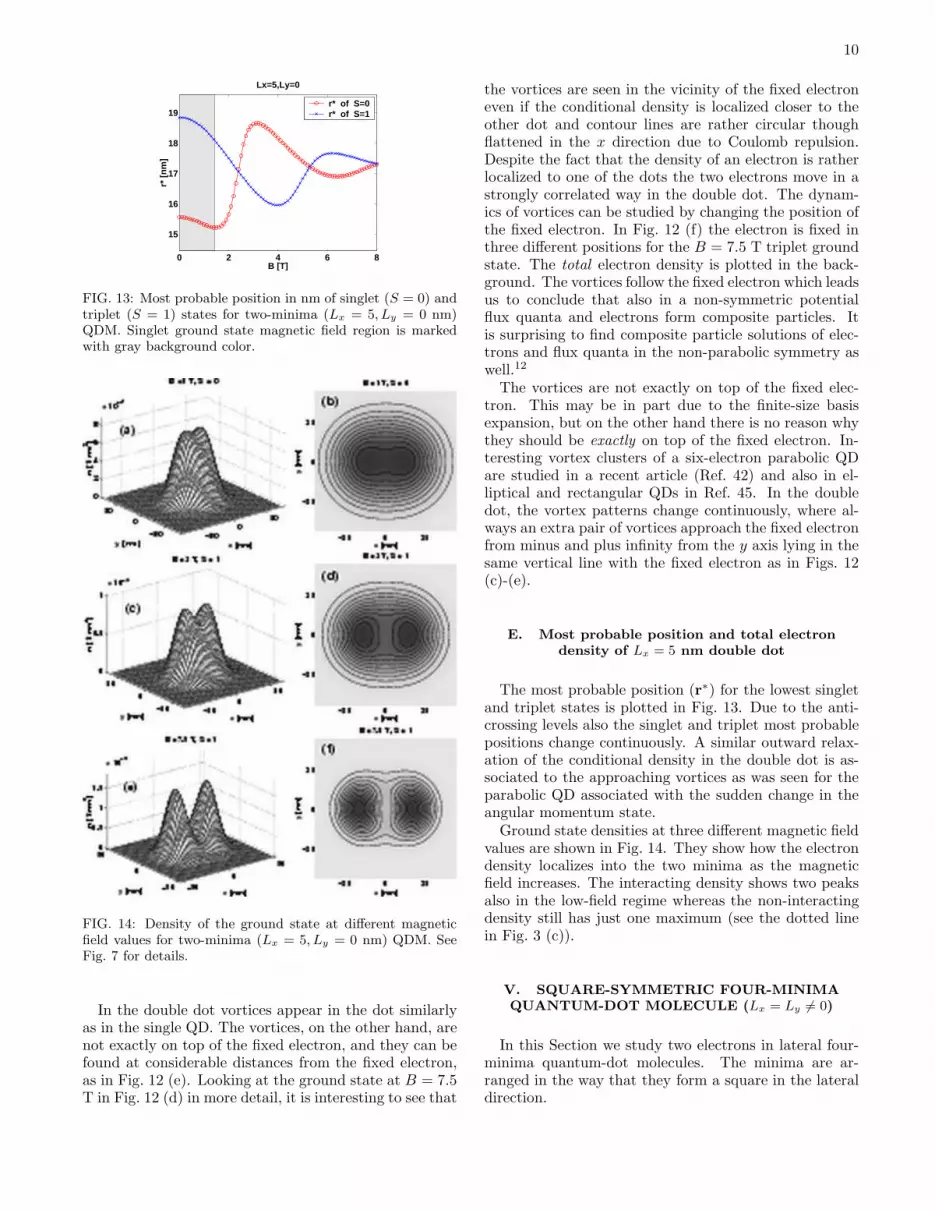
FIG. 13: Most probable position in nm of singlet (S = 0) andtriplet (S = 1) states for two-minima (Lx = 5, Ly = 0 nm)QDM. Singlet ground state magnetic field region is markedwith gray background color.

FIG. 14: Density of the ground state at different magneticfield values for two-minima (Lx = 5, Ly = 0 nm) QDM. SeeFig. 7 for details.

In the double dot vortices appear in the dot similarlyas in the single QD. The vortices, on the other hand, arenot exactly on top of the fixed electron, and they can befound at considerable distances from the fixed electron,as in Fig. 12 (e). Looking at the ground state at B = 7.5T in Fig. 12 (d) in more detail, it is interesting to see that

the vortices are seen in the vicinity of the fixed electroneven if the conditional density is localized closer to theother dot and contour lines are rather circular thoughflattened in the x direction due to Coulomb repulsion.Despite the fact that the density of an electron is ratherlocalized to one of the dots the two electrons move in astrongly correlated way in the double dot. The dynam-ics of vortices can be studied by changing the position ofthe fixed electron. In Fig. 12 (f) the electron is fixed inthree different positions for the B = 7.5 T triplet groundstate. The total electron density is plotted in the back-ground. The vortices follow the fixed electron which leadsus to conclude that also in a non-symmetric potentialflux quanta and electrons form composite particles. Itis surprising to find composite particle solutions of elec-trons and flux quanta in the non-parabolic symmetry aswell.12

The vortices are not exactly on top of the fixed elec-tron. This may be in part due to the finite-size basisexpansion, but on the other hand there is no reason whythey should be exactly on top of the fixed electron. In-teresting vortex clusters of a six-electron parabolic QDare studied in a recent article (Ref. 42) and also in el-liptical and rectangular QDs in Ref. 45. In the doubledot, the vortex patterns change continuously, where al-ways an extra pair of vortices approach the fixed electronfrom minus and plus infinity from the y axis lying in thesame vertical line with the fixed electron as in Figs. 12(c)-(e).

E. Most probable position and total electrondensity of Lx = 5 nm double dot

The most probable position (r∗) for the lowest singletand triplet states is plotted in Fig. 13. Due to the anti-crossing levels also the singlet and triplet most probablepositions change continuously. A similar outward relax-ation of the conditional density in the double dot is as-sociated to the approaching vortices as was seen for theparabolic QD associated with the sudden change in theangular momentum state.

Ground state densities at three different magnetic fieldvalues are shown in Fig. 14. They show how the electrondensity localizes into the two minima as the magneticfield increases. The interacting density shows two peaksalso in the low-field regime whereas the non-interactingdensity still has just one maximum (see the dotted linein Fig. 3 (c)).

V. SQUARE-SYMMETRIC FOUR-MINIMAQUANTUM-DOT MOLECULE (Lx = Ly 6= 0)

In this Section we study two electrons in lateral four-minima quantum-dot molecules. The minima are ar-ranged in the way that they form a square in the lateraldirection.

11

FIG. 15: Triplet-singlet energy difference (∆E = E↑↑ − E↑↓)as a function of magnetic field in square-symmetric (L = Lx =Ly) four-minima quantum dot molecule. See Fig. 9 for details.

A. Singlet-triplet splitting as a function of L

We study singlet and triplet states as a function ofmagnetic field and dot-dot separation. Fig. 15 (a) showsaltering singlet and triplet states as a function of mag-netic field. More frequent singlet-triplet changes are seenat greater separations between the dots (large L). Alsonotable is the large energy difference of the second sin-glet state to the triplet state. The second singlet alsopersists as a ground state to the greatest studied sep-aration L, which is not true in the double dot, if theZeeman energy is included (Fig. 15 (c)). In all studiedseparations L the magnetic field evolution of the Zeemancoupled four-minima QDM (Figs. (c) and (d)) followsthe same pattern. At small magnetic field values theground state is singlet, then triplet and again singlet ina small magnetic field window before the ground statechanges to triplet permanently. However, with large sep-arations L the system becomes spin-polarized at lowermagnetic field values, i.e. the border line of the secondsinglet and second triplet curves towards low-field regionwith increasing L.

We will now analyze the rapid changes of the singletand triplet states of four-minima QDM. Singlet-triplet(and triplet-singlet) transition points shift to lower mag-netic field values at greater L, where the area of the QDM(A) is effectively larger. If the transitions occur at effec-tively the same values of the magnetic flux (Φ = BA),the transitions should be seen at lower B when the areais larger. This explains why the border lines between sin-glet and triplet states curve towards lower B at greaterseparations between the dots.

The second singlet is seen as a ground state in theZeeman coupled system even at the very large distanceof L = 20 nm where the perturbation from a purely

parabolic potential is clear. However, in this type ofsquare- or ring-like potential spatially symmetric states(singlet) are energetically more favorable than in elon-gated potentials (double dot) where in general the spa-tially antisymmetric states (triplet) are favored withoutpaying too high price in Coulomb energy. Of course, asall energy scales are quite equal, the ground state is a del-icate balance between kinetic, confinement and Coulombenergies as a function of magnetic field.

B. Energy levels of Lx = Ly = 5 nm QDM

We will now focus on the Lx = Ly = 5 nm four-minimaQDM. The energy levels of non-interacting two-body, sin-glet and triplet states are plotted in Fig. 16 (a)-(c), re-spectively. In the square-symmetric four-minima QDMthe ground state levels do not anticross as in the dou-ble dot, instead crossing ground states of the same spinstate are seen, as in the single QD. However, the four-minima QDM is not circular symmetric and anticrossingsare still seen in the higher energy levels, which is not thecase with circular symmetric parabolic QD. Notice thatin the non-interacting spectra in Fig. 16 (a) many lev-els are degenerate at B = 0 for the four-minima QDM,whereas in the double dot the zero-field degeneracies aremostly lifted, see Fig.10 (a). Yet, many levels that aredegenerate in the single QD, Fig.4 (a), as function ofmagnetic field, are slightly split in the non-interactingenergy levels of four-minima QDM.

The singlet and triplet energies can be seen in the sameplot in Fig. 16 (d). The energy levels of the four-minimaQDM in Fig 16 (d) look very similar to single QD energylevels of Fig 4 (d). Even if the absolute values of energiesand transition points are different, the only notable dif-ferences between parabolic QD and four-minima QDMare the small bending at zero field of the third tripletlevel, near E ≈ 12.9 meV, and small anticrossing of theuppermost triplet level at B ≈ 1.3 T.

C. Singlet-triplet splitting and magnetization ofLx = Ly = 5 nm QDM

The energy difference between the lowest triplet andsinglet and the magnetization are plotted in Fig. 17.Now, as no anticrossings of ground states are present,the triplet-singlet energy difference shows peaks. In themagnetization we also observe sharp peaks whenever twoground states cross. Similar results are seen in a squarequantum dot with a repulsive impurity of Ref. 38 wherethe magnetization of two electrons in the dot shows sharptransitions since no anticrossings in the ground statesare present. On the other hand, in a square QD witheight electrons slightly rounded magnetization curves areseen.26 Therefore, if the circular symmetry of the con-finement is broken, the magnetization depends on thesymmetry of the confinement but also on the number of

12

FIG. 16: Energy levels of Lx = Ly = 5 nm four-minima QDM. See Fig. 4 for details.

FIG. 17: Triplet-singlet energy difference in (a) and magne-tization in (b) for Lx = 5 = Ly = 5 QDM. See Fig. 5 fordetails.

FIG. 18: (a)-(e) Contours of conditional densities |ψc(x, y)|2

and phase of the conditional wavefunction θc(x, y) in gray-scale for Lx = 5, Ly = 5 four-minima QDM. See Fig. 6 for de-tails. (f) contours of total electron density of the three-vortextriplet state are plotted in the background and positions ofthe vortices with the fixed electron in two different positions.

the electrons in the QD. It may not be straightforward todraw any conclusion about the underlying potential fromthe magnetization curves. Anticrossings, on the otherhand, are clear signatures of a broken circular symmetry.

0 2 4 6 8

14

15

16

17

18

19

20

21

B [T]

r* [n

m]

Lx=Ly=5

r* of S=0r* of S=1

FIG. 19: Most probable position in nm of singlet (S = 0)and triplet (S = 1) states for four-minima Lx = Ly = 5 nmQDM. Singlet ground state magnetic field region is markedwith gray background color.

D. Vortices of Lx = Ly = 5 nm QDM

We can identify the changes in the magnetization tothe increasing number of vortices in the two-electronQDM or to the increase of the expectation value of rela-tive angular momentum of the electrons. Vortex patternsand conditional densities are shown in Fig. 18. The mostprobable position is now found from the line connectingtwo minima diagonally.

ψc(x, y) =ΨS [(x, y), (x∗, y∗)]

ΨS[(−x∗,−y∗), (x∗, y∗)] , x∗ = y∗. (12)

At B = 0.7 T in (a) the conditional density is spread tothe area of three unoccupied dots with a peak in the fur-thermost dot on the diagonal from the fixed electron. Athigh magnetic field the density becomes more localizedcloser to the most distant minimum, in the diagonal fromthe fixed electron. However, the contours show that theconditional density is not as circularly symmetric as in adouble dot, but actually resembles more the conditionaldensity of the single parabolic QD. The peak in the con-finement potential at the origin seems not to affect theconditional density considerably when compared to thesingle QD. At high B the Coulomb repulsion forces elec-

13

FIG. 20: Density of the ground state at different magneticfield values for four-minima Lx = Ly = 5 nm QDM. SeeFig. 7 for details.

tron density to the outer edges of the confinement, whichmight not result in very different results when comparedto the single dot. However, the distance Lx = Ly = 5nm in the confinement is not particularly large and theperturbation from the parabolic confinement is not verylarge. On the other hand, altering singlet and tripletstates persist to the greatest studied distance (L = 20nm) between the dots of L = 20 nm where the perturba-tion from the parabolic confinement is clear.

The vortices appear in the four-dot QDM sequentiallyas a function of magnetic field. At low B the groundstate is a singlet with no vortices, then a triplet with onevortex, a singlet with two vortices and then a triplet with

three vortices. The singlet with four vortices in Fig. 18(e) is an excited state as the system becomes spin polar-ized after the two-vortex singlet state. The vortices arelocated in the diagonal going through the fixed electronposition, see Figs. 18 (c)-(e). The vortices seem to befurther away from the fixed electron (in the case of morethan one vortex) than in the single QD. This is also truein the double dot. This could be identified to repulsionbetween the vortices but it is difficult to assess since thelength scales are different due to different confinementstrength and also the basis causes some errors. However,with six electrons in a parabolic confinement one can seea clear repulsion between the vortices.42

Vortex dynamics of the three-vortex solution is studiedby changing the position of the fixed electron in Fig. 18(f). Total electron density of the same state is plottedin the background of Fig. 18 (f). Vortices are seen tofollow the fixed electron also in the four-minima QDM.However, in the four-minima QDM the vortices are fur-ther away from the fixed electron as the distance fromthe origin increases.

E. The most probable position and density ofLx = Ly = 5 nm QDM

The most probable positions of the lowest singlet andtriplet states of the four-minima QDM (Fig. 19) showvery similar behavior as the single QD. Only the mostprobable positions are on average roughly 2 nm greaterat all field strengths compared to the single QD (sizeof the QDM is larger compared to single QD). Otherwisecontinuously decreasing r

∗ shows a jump when the lowestsinglet (or triplet) state changes.

Ground state densities and contours are plotted inFig. 20. Starting from a rather flat density at low fields,a hole begins to form in the center as the magnetic fieldis increasing. The electron density localizes into a nar-rowing ring around the origin. However, compared to theparabolic QD, there are peaks forming in the four cornersof the density, instead of a smooth density ring. Also thedensity looks more square-like in all of the contours.

VI. RECTANGULAR FOUR-MINIMAQUANTUM DOT MOLECULE (Lx 6= Ly 6= 0)

In this Section we examine the triplet-singlet energydifference, energy eigenlevels, magnetization, vortices,the most probable positions, and densities of four-minimaQDM with rectangular positioning of the QD minima inthe lateral plane.

14

FIG. 21: Triplet-singlet energy difference (∆E = E↑↑−E↑↓)as a function of magnetic field in rectangular-symmetric four-minima quantum dot molecule. Lx is fixed to 5 nm and Ly

is varied from 0 to 20 nm. Therefore at Ly = 0 we haveLx = 5 nm double dot and at Ly = 5 nm it is the square-symmetric four-minima QDM. The energy difference is plot-ted as a function of Ly and magnetic field in (a) withoutZeeman energy and in (c) with the Zeeman energy included(∆E = E↑↑ + EZ − E↑↓). In (b) and (d) the ground stateregions of the singlet and triplet states are plotted as functionof B and Ly , without and with Zeeman energy, respectively.

A. Singlet triplet splitting as function of Ly forfixed Lx = 5 nm rectangular QDM

The triplet-singlet energy difference of the rectangularQDM is plotted in Fig. 21. The distance between theminima in the x direction is fixed while the distance in they direction is varied. We set Lx = 5 nm and vary Ly fromzero to 20 nm. Therefore, at Ly = 0 we have a Lx = 5 nmdouble dot, and at Ly = 5 nm we have the Lx = Ly = 5nm square-symmetric four-minima QDM studied in thepreceding section. The smooth surface in Fig. 21 is dueto anticrossing ground states similarly as in the doubledot. The anticrossings in the lowest levels of the singletand triplet states are again present if the symmetry isdistorted from a square to a rectangular symmetry, seethe energy levels in Fig. 22. The only sharp peaks inFig. 21 (a) and (c) correspond to rectangular symmetricQDM at Lx = Ly = 5 nm.

One can also see that as a function of magnetic fieldsinglet and triplet states do not change as rapidly as inthe square-symmetric four-minima QDM. Interestingly,the third singlet region terminates around Ly ≈ 15 nm.So at sufficiently large distance between the two Lx = 5nm double dots the singlet state is no longer favorableeven if the Zeeman term is excluded. In the case of adouble dot in Ref. 12 it was not possible to say whetherthe second singlet state would terminate at greater dis-tances between the dots, but for two double dots the third

singlet region clearly terminates.If the Zeeman term is included (Figs. 21 (c) and (d))

the second singlet state can only be observed in a smallregion where the rectangular four-minima QDM is closeto square symmetry (near Ly = 5 nm). Actually theenergy difference has its maximum, as function of Ly,at the square symmetry. If we follow the energy differ-ence at zero magnetic field as a function of Ly, it firstincreases reaching the maximum at Ly = 5 nm and thenit decreases again when Ly is increased.

The stability of the singlet states (and also tripletstates) in the square-symmetric QDM can be understoodfrom the relatively high energy of the triplet state (orsinglet) near the peak in ∆E. In the square symme-try the degenerate energy levels at the crossing point areenergetically very unfavorable. In rectangular symme-try degeneracies are lifted (anticrossings), which lowersthe energy of the other spin type and also reduces theenergy difference, ∆E. Thus the energy differences arealways smaller in the rectangular symmetry when anti-crossings are present. The Jahn-Teller theorem statesthat any non-linear molecular system in a degenerateelectronic state will be unstable and will undergo a dis-tortion to form a system of lower symmetry and lowerenergy, thereby removing the degeneracy.48 In a QDM,the system cannot, of course, lower the symmetry of theexternal confinement spontaneously to lift the degenera-cies, but the large triplet-singlet energy differences inthe square-symmetric QDM can be understood via Jahn-Teller effect: If the symmetry is lowered, degeneracies arelifted and smaller triplet-singlet energy differences are ob-served.

B. Energy levels of Lx = 5, Ly = 10 nm QDM

We will now study rectangular Lx = 5, Ly = 10 nmQDM in more detail. Fig. 22 (b) and (c) reveal manyanticrossings in the interacting two-body spectra of Lx =5, Ly = 10 nm QDM, both in the ground states and alsoin the excited states. Many features look similar as in thedouble dot spectra in Fig. 10 but the anticrossing gapsare bigger here due to the greater separations betweenthe dots (greater deviation from the circular symmetry).Fig. 22 (d) shows singlet and triplet energy levels in thesame plot. The second singlet becomes very close to thetriplet near B = 5 T, but the triplet remains the groundstate.

C. Singlet-triplet splitting and magnetization ofLx = 5, Ly = 10 nm QDM

The energy difference of triplet and singlet states isplotted in Fig. 23 (a). The magnetization in Fig. 23(b) show first a sharp peak which corresponds to singlettriplet transition. The next change is from the one-vortextriplet to the three-vortex triplet and as these two states

15

FIG. 22: Energy levels of Lx = 5, Ly = 10 nm rectangular four-minima QDM. See Fig. 4 for details.

FIG. 23: Triplet-singlet energy difference (a) and magneti-zation (b) in Lx = 5, Ly = 10 nm rectangular four-minimaQDM. Magnetization is given in the units of effective Bohrmagnetons µ∗

B = e~/2m∗.

FIG. 24: (a)-(e) contours of conditional densities |ψc(x, y)|2

and phase of the conditional wavefunction θc(x, y) in gray-scale for Lx = 5, Ly = 10 four-minima QDM. See Fig. 6 fordetails. (f) contours of total electron density of the three-vortex triplet state are plotted in the background and posi-tions of the vortices with the fixed electron in three differentpositions.

anti-cross we see continuous increase of the magnetiza-tion before it starts to decrease again due to the contrac-tion of the electron density. It is interesting that afterthe bump the interacting magnetization has very similardependence on the magnetic field as the non-interacting

FIG. 25: Density of the ground state at different magneticfield values for Lx = 5, Ly = 10 nm rectangular four-minimaQDM. See Fig. 7 for details.

magnetization. At high enough magnetic field the elec-trons are localized into individual double dots and havesingle-particle properties and the spatial extents in theinteracting and non-interacting systems are not very dif-ferent (see Eq. (6)). However, the electrons may movein a correlated way even if they are localized into one ofthe double dots. One should remember that there is also

16

0 2 4 6 8

17

18

19

20

21

B [T]

r* [n

m]

Lx=5,Ly=10

r* of S=0r* of S=1

FIG. 26: Most probable position in nm of singlet (S = 0) andtriplet (S = 1) states for rectangular-symmetric four-minima(Lx = 5, Ly = 10 nm) QDM. Singlet ground state (magneticfield) region is marked with gray background color.

the paramagnetic part in the magnetization, but this isconstant for a given state, if the the angular momentumis a good quantum number, and does not depend on themagnetic field. Of course, in a non-circular symmetrythe paramagnetic magnetization may not be constant asa function of magnetic field.

D. Vortices of Lx = 5, Ly = 10 nm QDM

The phase information and the conditional densities ofthe rectangular four-minima QDM are shown in Fig. 24.The most probable position lies now on the y axis. An-other possibility would be to have the most probable po-sition on a line connecting the two minima diagonally.However, as the other double dot is left with just oneelectron and the distance of Lx = 5 nm is so small thatthe single-particle density is not localized to the minimaof the double dot. So the most probable position is inthe y axis. In rectangular symmetry correlations forcethe one electron to one of the double dots. With smallLx’s conditional density shows a peak at x = 0 as in thenon-interacting two-body density in Fig. 3.

The conditional density becomes more localized as themagnetic field increases. The vortices appear sequen-tially in the QDM. The second and third singlet states(in Fig. 24 (c) and (e)) are not ground states as the sys-tem becomes spin-polarized after the first singlet-triplettransition. There is again a repulsion between the vor-tices. Interesting is to note that in (e) the two moredistant vortices are positioned much closer to the fixedelectron when compared to the double dot of Fig. 12 (e).The white and dark regions near the borders of Fig. 24(e) show the shades of phase boundaries of more distantvortices (not visible in the figure).

Vortex dynamics is studied in Fig. 24 (f) for the threevortex triplet (at B = 6.5 T). The electron is fixed atthree different positions and the total electron density ofthe same state is plotted in the background. One vortex,or Pauli vortex, is always on top of the fixed electron

and the two additional vortices are symmetrically on thesides of the fixed electron. As the fixed electron is movedfrom the origin to the direction of the positive y axis, thevortices aside become closer to the fixed electron.

E. Total electron density and the most probablepositions of Lx = 5, Ly = 10 nm QDM

Ground state electron densities in Fig. 25 show a lo-calization into two double dots as the magnetic field isincreased. If the densities would be rotated by 90 de-grees they would resemble very much two-minima QDM(double dot) densities of Fig. 14. The smaller displace-ment (Lx = 5 nm) in the four-minima QDM potentialhas a much smaller effect than the larger displacement(Ly = 10 nm) because electrons localize into the doubledots (with Lx = 5 nm) separated from each other witha distance d = 2Ly = 20 nm. Therefore electron densityof rectangular four-minima QDM effectively resembles ofthat of a two-minima QDM (double dot). This is truefor interacting two-electron system.

The most probable positions of the lowest singlet andtriplet states are shown in Fig. 26. Continuously chang-ing r

∗ (i.e. no jumps) is due to anticrossing states wheresymmetry of a state (and also r

∗) changes continuously.Interesting is the strong suppression of the oscillationsof r

∗ at greater B. At large magnetic field the electronslocalize into a distant double dots and interaction effects(like changing angular momentum states in parabolicQD) have a smaller impact on the properties of the two-electron system. The effect is quite different for parabolicQD and square-symmetric four-minima QDM where thelocalization of electron density is not so strong due to thenature of the confinement potential.

VII. ANALYSIS OF THE RESULTS AND THEIRRELEVANCE TO EXPERIMENTS

A. Role of symmetry in quantum dot confinement

We start our analysis of the data presented above fromthe measurable quantities. One such observable is thetotal energy for ground and excited states as a functionof the magnetic field, as well as the magnetization. Toease the comparison, these are collected in Fig. 27. Themost striking feature is that the data of the the square-symmetric four-minima QDM is very similar to the oneof the single parabolic dot. On the other hand, the dataof the double dot resemble the one of a rectangular four-minima QDM. The reason behind the similarities of thesepairs is the symmetry. The square-symmetric and circu-larly symmetric cases have higher symmetries than therectangular ones. One can study this in detail by split-ting the total Hamiltonian of Eq. (1) to two parts asH = H0 + HI , where H0 is the Hamiltonian of theparabolic case (Lx = Ly = 0), and the impurity Hamilto-

17

FIG. 27: Three lowest singlet and triplet energy levels andmagnetization for all studied quantum dot confinements.

nian HI contains the terms from finite Lx and Ly values,see Eq. (3). If we now have a high symmetry in the sys-tem, meaning Lx = Ly, one can see that the HI does notcouple the eigenstates of H0 that have a different sym-metry. On the other hand, in the case with Lx 6= Ly, HI

has a lower symmetry and more of the symmetries of H0

are broken. Due to this, states with different symmetryare coupled. This leads to anticrossings in the energiesas seen in Fig. 27, where also the crossings of the high-symmetry cases are seen. One can estimate the strengthof the symmetry-lowering part from the anti-crossing gapin energy, as in the point where the energies would cross,one has in the first approximation a Hamiltonian matrix:

H =

(

E0 Eδ

Eδ E0

)

, (13)

where E0 is the energy at middle of the gap, and 2Eδ isthe width of the gap.

The magnetization curve for the low- and high-symmetry cases are also very different, see Fig. 27.A common feature in all these cases is the sharp in-crease in magnetization at the point where the total spinof the ground-state changes. On the other hand, thelow-symmetry anticrossings of the energy result smoothchanges in magnetization, whereas the high-symmetrydata show sudden jumps.

These findings indicate that it is rather difficult to ob-tain detailed information of the system based on the en-ergetics and the magnetization. The symmetry of thesystem can be extracted, but not much beyond that. Forlarger particle numbers, more and more of the correlationeffects can be captured by the mean-field level. The effec-tive potential has, due to the Hartree potential, a highersymmetry than the mere external potential.5 This resultsin less details to both energetics and the magnetization.

A similar role of the symmetry can be seen on the non-measurable quantities, like the densities. On the otherhand, the vortices are more delicate. This is because theydepend linearly on the wave function, unlike densities andenergies that are second order.

B. Exchange of two spins

The idea of double dot spin-swap operations in quan-tum computing14 lies in the coherent rotation of two ini-tially isolated spins. Starting with, say, spin-up elec-tron in the left and spin-down electron in the right dot:|↑〉L|↓〉R and rotating spins to opposite order: |↓〉L|↑〉R.These would be initial and final states of the system. Co-herent rotation between initial and final states requiresentangled spin states like spin-singlet |S〉 = (|↑〉L|↓〉R −|↓〉L|↑〉R)/

√2 and triplet |T0〉 = (|↑〉L|↓〉R+|↓〉L|↑〉R)/

√2

whereas the other two triplet states |T+〉 = |↑〉L|↑〉R and|T−〉 = |↓〉L|↓〉R are not conceivable as they have iden-tical spins. The states described above are only for thespin-part of the wave function but of course the spatialpart, discussed extensively in this paper for singlet andtriplet eigenstates, must be modified along with the ro-tation.

In the simplified Heisenberg picture, rotation dependsonly on the singlet-triplet splitting energy, J = ∆E =E↑↑−E↑↓, or exchange coupling of two spins.14 Hubbard-type models can be used to study time evolution of a lit-tle bit more elaborate states.15,16 To fully investigate thecoherent rotation of two-electron system, it would be bet-ter to start with initially separated electrons (that can beconstructed from many-body wave functions) and studythe time evolution of the state in the exact many-bodybasis instead of using some simplified models. However,tuning J with dot-dot separation at small magnetic fields,the spin rotations can be quite safely modelled within theHeisenberg picture. At high magnetic fields, on the otherhand, electrons in lateral double dots form finite quan-

18

tum Hall-like composite-particle states of electrons andflux quanta, as shown in this study and in previous stud-ies.12,17 Therefore, the coherent spin rotations at highB may be quite different from zero B rotations, even ifJ could have exactly same value for high-B and zero-Bstates. These states are of course of great scientific in-terest as their own, but from the perspective of coherenttwo-spin rotations they may function quite differently assuggested by the Heisenberg or Hubbard models. Electriccontrol of J with dot-dot separation may also be advan-tageous in other perspectives because magnetic fields aremore difficult to apply locally.

C. Comparisons to experiments

In very recent experiments Petta et al. demonstratea coherent rotation of two spins between singlet |S〉 andtriplet |T0〉 states in a lateral double dot device.25 Theystart the operation from singlet state in single QD andthen isolate two opposite spins in separated dots wherethe singlet-triplet splitting vanishes and no tunneling isallowed between the two dots. Coherent rotation is per-formed by bringing the two dots closer allowing smallbut finite energy splitting J between |S〉 and |T0〉 states.Probability of finding singlet is measured as a function ofgate operation time. Fig. 9 (a) of this study shows cal-culated singlet-triplet splitting as a function of dot-dotseparation and magnetic field. Following the zero mag-netic field line one and see how the singlet-triplet splittingdecreases as a function of increasing dot-dot separation.Fixing B = 0.1 T, as in the experiment, for single dot(L = 0) we have J = 1.16 meV and for double dot atthe greatest interdot distance studied (d = 2L = 40 nm)we have J = 0.16 meV. Petta et al.25 find three timessmaller value in single QD (J = 0.4 meV) as our calcula-tions. This is simply a consequence of different quantumdot confinement energy ~ω0.

Lee et al. studied experimentally singlet-triplet split-ting as a function of magnetic field in silicon two-electrondouble dot.18 The measurements show very similar dataas our results. The first singlet-triplet transition is re-solved clearly in the experiment in accordance to ourcalculations. Decreasing the coupling between the dotsresults in a small shift of J = 0 to low fields as in our re-sults represented in Fig. 9. The high-field regime, wherewe would expect to find small J and even possibly a pos-itive J , which would correspond second singlet ground

state, is not measured to very high field strengths. How-ever, to fully compare our results to the measurements onsilicon double dots we should recalculate our data withsilicon effective mass and dielectric constant.

Brodsky et al. 13 were the first to measure ground stateenergy levels of a lateral two-electron double dot as afunction of magnetic field. Even if they did not concen-trate on two-electron case particularly, the line for twoelectrons is clearly visible in their data showing also akink indicating the singlet-triplet transition.

Magnetization is very difficult to measure directly forjust two electrons. However, indirect methods and directmethods with large arrays of individual few-electron dotsmay provide interesting experimental results.34,35 Even ifit is difficult to compare existing measurements of manyelectron dots to our two-electron system, the double dotmeasurements of Oosterkamp et al. 34 show similar typeof anticrossings as our calculated magnetization curves.

VIII. SUMMARY

In summary, we have thoroughly studied different lat-eral two-electron quantum-dot molecules. All our exactdiagonalization calculations were performed for closelycoupled quantum dots. Many-body electron wave func-tions were allowed to extend over the whole system. Wehave analyzed how the physical properties change whena deviation or disorder is introduced in the confinementpotential of the symmetric quantum dot. We have calcu-lated measurable quantities such as energy levels, singlet-triplet splitting, and magnetization as a function of mag-netic field strength. The measurable quantities were fur-ther analyzed by calculating non-measurable quantitiessuch as phase vortices and conditional densities. We havealso compared the properties of non-interacting electronsto interacting ones in quantum dot molecules to separatethe effects of the non-circular confinement potential andinteractions.

Acknowledgments

This work has been supported by the Academy of Fin-land through its Centers of Excellence Program (2000-2005).

∗ Corresponding author: M. Helle before M. Marlo; Elec-tronic address: Meri.Helle@hut.fi

1 T. Chakraborty and P. Pietilainen, The Quantum Hall Ef-

fects: Fractional and Integral, (Springer, Berlin, 1995).2 L. Jacak, P. Hawrylak, and A. Wojs, Quantum Dots

(Springer, Berlin, 1998).3 P. A. Maksym and Tapash Chakraborty, Phys. Rev. Lett.

65, 108 (1990).4 M. Hochgrafe, Ch. Heyn, and D. Heitmann, Phys. Rev. B

63, 035303 (2001).5 M. Marlo, A. Harju, and R. M. Nieminen, Phys. Rev. Lett.

91, 187401 (2003).6 T. Chakraborty, V. Halonen, and P. Pietilainen, Phys.

Rev. B 43, R14289 (1991).

19

7 D. Pfannkuche and R. R. Gerhardts, Phys. Rev. B 44,R13132 (1991).

8 A. V. Madhav and T. Chakraborty, Phys. Rev. B 49, 8163(1994).

9 I. Magnusdottir and V. Gudmundsson, Phys. Rev. B 60,16591 (1999).

10 C. A. Ullrich and G. Vignale, Phys. Rev. B 61, 2729 (2000).11 Tapash Chakraborty and Pekka Pietilainen, Phys. Rev.

Lett. 95, 136603 (2005).12 A. Harju, S. Siljamaki, and R. M. Nieminen, Phys. Rev.

Lett. 88, 226804 (2002).13 M. Brodsky, N. B. Zhitenev, R. C. Ashoori, L. N. Pfeiffer,

and K. W. West, Phys. Rev. Lett. 85, 2356 (2000).14 D. Loss and D. P. DiVincenzo, Phys. Rev. A 57, 120

(1998).15 G. Burkard, D. Loss, and D. P. DiVincenzo Phys. Rev. B

59, 2070 (1999).16 John Schliemann, Daniel Loss, and A. H. MacDonald,

Phys. Rev. B 63, 085311 (2001).17 V. W. Scarola and S. Das Sarma, Phys. Rev. A 71, 032340

(2005).18 S. D. Lee, S. J. Kim, J. S. Kang, Y. B. Cho, J. B. Choi,

Sooa Park, S.-R. Eric Yang, S. J. Lee, T. H. Zyung,cond-mat/0410044.

19 A. K. Huttel, S. Ludwig, H. Lorenz, K. Eberl, and J. P.Kotthaus, Phys. Rev. B 72 081310(R) (2005).

20 J. M. Elzerman, R. Hanson, J. S. Greidanus, L. H. Willemsvan Beveren, S. De Franceschi, L. M. K. Vandersypen,S. Tarucha, and L. P. Kouwenhoven, Phys. Rev. B 67,161308(R) (2003).

21 A. C. Johnson, J. R. Petta, J. M. Taylor, A. Yacoby, M. D.Lukin, C. M. Marcus, M. P. Hanson, and A. C. Gossard,Nature 435, 925 (2005).

22 F. H. L. Koppens, J. A. Folk, J. M. Elzerman, R. Hanson,L. H. Willems van Beveren, I. T. Vink, H. P. Tranitz, W.Wegscheider, L. P. Kouwenhoven, and L. M. K. Vander-sypen, Science 309, 1346 (2005).

23 J. M. Elzerman, R. Hanson, L. H. Willems van Beveren, B.Witkamp, L. M. K. Vandersypen, and L. P. Kouwenhoven,Nature 430, 431 (2004).

24 R. Hanson, L. H. Willems van Beveren, I. T. Vink, J.M. Elzerman, W. J. M. Naber, F. H. L. Koppens, L. P.Kouwenhoven, and L. M. K. Vandersypen, Phys. Rev. Lett.94, 196802 (2005).

25 J. R. Petta, A. C. Johnson, J. M. Taylor, E. A. Laird, A.Yacoby, M. D. Lukin, C. M. Marcus, M. P. Hanson, andA. C. Gossard, Science 309, 2180 (2005).

26 E. Rasanen, A. Harju, M. J. Puska, and R. M. Nieminen,Phys. Rev. B 69, 165309 (2004).

27 P. S. Drouvelis, P. Schmelcher and F. K. Diakonos, J. of

Phys.: Condens. Matter 16, 3633 (2004).28 P. S. Drouvelis, P. Schmelcher and F. K. Diakonos, Phys.

Rev. B 69, 035333 (2004).29 P. S. Drouvelis, P. Schmelcher and F. K. Diakonos, Phys.

Rev. B 69, 155312 (2004).30 B. Szafran, F. M. Peeters, S. Bednarek, and J. Adamowski,

Phys. Rev. B 69, 125344 (2004).31 B. Szafran, F. M. Peeters, S. Bednarek, Phys. Rev. B 70,

205318 (2004).32 B. Szafran and F. M. Peeters, Phys. Rev. B 71, 245314

(2005).33 R. Ugajin, Physica B 253, 92 (1998).34 T. H. Oosterkamp, S. F. Godijn, M. J. Uilenreef, Y. V.

Nazarov, N. C. van der Vaart, and L. P. Kouwenhoven,Phys. Rev. Lett. 80, 4951 (1998).

35 M. P. Schwarz, D. Grundler, M. Wilde, C. Heyn, and D.Heitmann, J. Appl. Phys. 91, 6875 (2002).

36 M. P. Schwarz, D. Grundler, Ch. Heyn, D. Heitmann, D.Reuter, and A. Wieck, Phys. Rev. B 68, 245315 (2003).

37 P. A. Maksym and Tapash Chakraborty, Phys. Rev. B 45,R1947 (1992).

38 Weidong Sheng, and Hongqi Xu, Physica B 256-258, 152(1998).

39 J. I. Climente, J. Planelles, and J. L. Movilla, Phys Rev.B 70, 081301(R) (2004).

40 I. Magnusdottir and V. Gudmundsson, Phys. Rev. B 61,10229 (2000).

41 A. Aldea, V. Moldoveanu, M. Nita, A. Manolescu, V.Gudmundsson, and B. Tanatar, Phys. Rev. B 67, 035324(2003).

42 H. Saarikoski, A. Harju, M. J. Puska, R. M. Nieminen,Phys. Rev. Lett. 93, 116802 (2004).

43 M. B. Tavernier, E. Anisimovas, and F. M. Peeters, Phys.Rev. B 70, 155321 (2004).

44 M. Toreblad, M. Borgh, M. Koskinen, M. Manninen, andS. M. Reimann Phys. Rev. Lett. 93, 090407 (2004).

45 H. Saarikoski, S. M. Reimann, E. Rasanen, A. Harju, andM. J. Puska, Phys. Rev. B 71, 035421 (2005).

46 H. Saarikoski and A. Harju, Phys. Rev. Lett. 94, 246803(2005).

47 M. Marlo-Helle, A. Harju, and R. M. Nieminen, Physica E26, 286 (2005).

48 H. A. Jahn and E. Teller, Proc. R. Soc. London A 161,220 (1937).

49 J. K. Jain and T. Kawamura, Europhys. Lett. 29, 321(1995).

50 A. Harju, B. Barbiellini, R. M. Nieminen, and V. A.Sverdlov, Physica B 255, 145 (1998).