Embed Size (px)
Citation preview

arX
iv:h
ep-t
h/93
1013
6v2
28
Feb
1995
Two Ising Models Coupled to 2–Dimensional
Gravity
Mark Bowick, Marco Falcioni,
Geoffrey Harris and Enzo Marinari(∗)
Dept. of Physics and NPAC,
Syracuse University,Syracuse, NY 13244-1130, USA
bowick falcioni gharris @npac.syr.edu
(∗): and Dipartimento di Fisica and INFN,
Universita di Roma Tor Vergata
Viale della Ricerca Scientifica, 00173 Roma, Italy
September 25, 2013
Abstract
To investigate the properties of c = 1 matter coupled to 2d–gravitywe have performed large-scale simulations of two copies of the IsingModel on a dynamical lattice. We measure spin susceptibility and per-colation critical exponents using finite-size scaling. We show explic-itly how logarithmic corrections are needed for a proper comparisonwith theoretical exponents. We also exhibit correlations, mediatedby gravity, between the energy and magnetic properties of the twoIsing species. The prospects for extending this work beyond c = 1 areaddressed.
1

1 Introduction
There is at present considerable analytic understanding of how conformalmatter with central charge (c) less than or equal to one couples to two-dimensional gravity [1]. These c ≤ 1 models are relevant both as non-criticalstring theories and as novel statistical mechanical systems describing matteron a dynamical substrate lattice. The relation of these models to quantumLiouville theory [2] allows one to compute the shift in the scaling dimen-sion of physical operators due to the coupling to 2d-gravity. This shift isdetermined solely by the scaling dimension of the operator in the absence ofgravity (i.e on a fixed lattice) and the central charge of the theory. Given thedressed scaling dimensions one can compute critical exponents of thermody-namic observables related to correlation functions. Through the mapping ofthese systems onto matrix models it is even possible to incorporate topologychange by performing the entire sum over topologies in the so-called double-scaling limit. This beautiful state of affairs falls apart for central chargeexceeding one1. In this case the methods of Liouville theory appear to fail -in particular they predict complex critical exponents. The vanishing of themass of the dressed identity operator (the tachyon) at c = 1 suggests theonset of an instability in the worldsheet geometry. Based on this, it is widelybelieved that c > 1 no longer describes a continuum theory of surfaces [4].Since no models have been solved in this regime, it would be valuable toapply numerical techniques to see if c > 1 models appear to be qualitativelydifferent than those with c < 1.
A simple class of models to test our understanding of these issues isprovided by multiple copies of the Ising model on a dynamical lattice. EachIsing model has c = 1
2. A model with n individual copies then has c = n/2.
For a single Ising model (n = 1) on a dynamical lattice the critical exponentsmay be computed analytically via a mapping of the model onto a particular2-matrix model (with one matrix representing spin up and the other spindown) [5, 6]. The model has a third order rather than a second order phasetransition. Without the coupling to gravity the partition function of then-Ising model would simply be the n–th power of the single Ising modelpartition function, since the spins of different copies are independent. The
1More precisely when the quantity c − 24∆ > 1, where ∆ is the conformal weight ofthe lowest-weight state in the theory [3].
3

interaction with gravity, however, induces an effective interaction betweenspins of different species (copies). Spins of different species effectively interactthrough the dynamical lattice. Brezin and Hikami [7, 8, 9] have studied anequivalent 2n-matrix model realization of this system in perturbation theoryin the cosmological constant, without any apparent anomaly setting in atc = 1. Similarly Monte-Carlo studies of multiple–Ising and multiple–Pottsmodels on dynamically-triangulated random surfaces (DTRS) do not uncoverdramatic changes as c passes through one [10, 11, 12].
On the numerical side it is important that we understand the transitioncase c = 1 before plunging into the regime c > 1. This is the motivationfor the work presented in this paper on large-scale DTRS simulations of then = 1 and n = 2 Ising model coupled to 2d-gravity. In the n = 2 case theformalism of KPZ allows a computation of the relevant critical exponents,which we can consequently compare to the numerical results extracted fromfinite-size scaling and direct fits. The exact solution of the single-Ising modelalso provides a direct check that the discrete DTRS algorithm is reproduc-ing continuum behavior for the lattice sizes simulated and that the numericalanalysis methods employed are adequate. The n = 2 (c = 1) case is consider-ably more complicated than the n = 1 case because of logarithmic violationsof scaling. Here the extensive work on c = 1 matrix models provides anessential clue [13]. It allows us to identify the appropriate scaling variablethat replaces the cosmological constant. With this in hand we are able tocompare the results of our large-scale DTRS Monte-Carlo simulations withthe predictions of KPZ.
Similar issues are also addressed in a companion paper [14] in which per-colation coupled to gravity with c = 0, 1/2, 1 and c > 1 matter is examinedin much detail. The nature of finite size effects in simulations of two dimen-sional gravity plays a central role in that paper, as it does here. We shallshow how the percolation results for Gaussian matter in [14] are consistentwith those obtained in the two species Ising model discussed here.
The outline of the rest of the paper is as follows. In section 2 we give atheoretical discussion of c = 1 conformal matter coupled to 2d-gravity, with aderivation of the critical exponents we will be comparing with our numericalsimulations and a discussion of logarithmic violations of scaling. In section 3we present our numerical methods and results including a comparison withtheoretical expectations. Finally, in section 4, we conclude with a discus-sion of the origin of logarithmic corrections to scaling and the prospects for
4
extending this work to the regime c > 1 that this implies.
2 Theoretical Predictions
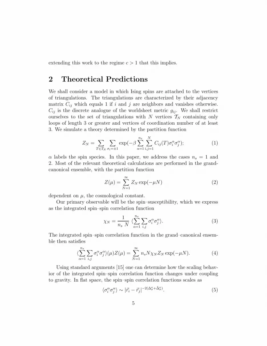
We shall consider a model in which Ising spins are attached to the verticesof triangulations. The triangulations are characterized by their adjacencymatrix Cij which equals 1 if i and j are neighbors and vanishes otherwise.Cij is the discrete analogue of the worldsheet metric gij. We shall restrictourselves to the set of triangulations with N vertices TN containing onlyloops of length 3 or greater and vertices of coordination number of at least3. We simulate a theory determined by the partition function
ZN =∑
T∈TN
∑
σi=±1
exp(−βns∑
α=1
N∑
i,j=1
Cij(T )σαi σα
j ); (1)
α labels the spin species. In this paper, we address the cases ns = 1 and2. Most of the relevant theoretical calculations are performed in the grand-canonical ensemble, with the partition function
Z(µ) =∞∑
N=1
ZN exp(−µN) (2)
dependent on µ, the cosmological constant.Our primary observable will be the spin–susceptibility, which we express
as the integrated spin–spin correlation function
χN =1
ns N〈
ns∑
α=1
∑
i,j
σαi σα
j 〉. (3)
The integrated spin–spin correlation function in the grand–canonical ensem-ble then satisfies
〈ns∑
α=1
∑
i,j
σαi σα
j 〉(µ)Z(µ) =∞∑
N=1
nsNχNZN exp(−µN). (4)
Using standard arguments [15] one can determine how the scaling behav-ior of the integrated spin–spin correlation function changes under couplingto gravity. In flat space, the spin–spin correlation functions scales as
〈σαi σα
j 〉 ∼ |~ri − ~rj |−2(∆oσ+∆o
σ). (5)
5

The weight ∆oσ = ∆o
σ = 1/16 is dressed by gravity in a theory of centralcharge c according to the KPZ formula [2]
(∆σ − ∆oσ) =
(
1 +1
12
(√1 − c −
√25 − c
)√1 − c
)
∆σ(1 − ∆σ). (6)
This dressed weight determines the scaling of the integrated spin–spin cor-relation function with µ on surfaces of genus h:
〈∑
α
∑
i,j
σαi σα
j 〉(µ)Z(µ) ∼ (µ − µc)2(−1+∆σ)+(2−γs)(1−h) (7)
(the −1 before the dressed weight accounts for the integrations of i and jover the surface) with
γs =1
12
(
c − 1 −√
(25 − c)(1 − c))
. (8)
The above relations and
ZN ∼ N−1+(γs−2)(1−h) (9)
yield the finite-size scaling relation
χN ∼ Nγ/νdH , (10)
withγ/νdH = 1 − 2∆σ. (11)
This is the scaling law that we shall verify numerically. The susceptibilityscales as χ ∼ (β−βc)
−γ , the correlation length (governed by the decay of thespin–spin correlation function) obeys ξ ∼ (β − βc)
−ν and dH is the intrinsicHausdorff dimension of the random surface being considered.
Assuming the standard scaling hyperscaling relation α = 2 − νdH , wecan also predict the value of γ. The specific heat scales as Nα/νdH . Then byapplying the reasoning used to arrive at (11) to the two-point function of theenergy operator ε, one finds α/νdH equals 1 − 2∆ε, where ∆ε is the dressedweight of the energy operator. It then follows that
γ =(1 − 2∆σ)
(1 − ∆ε). (12)
6
One obtains ∆ε through the KPZ formula (6), substituting the bare energyweight ∆o
ε = 1/2 for ∆oσ.
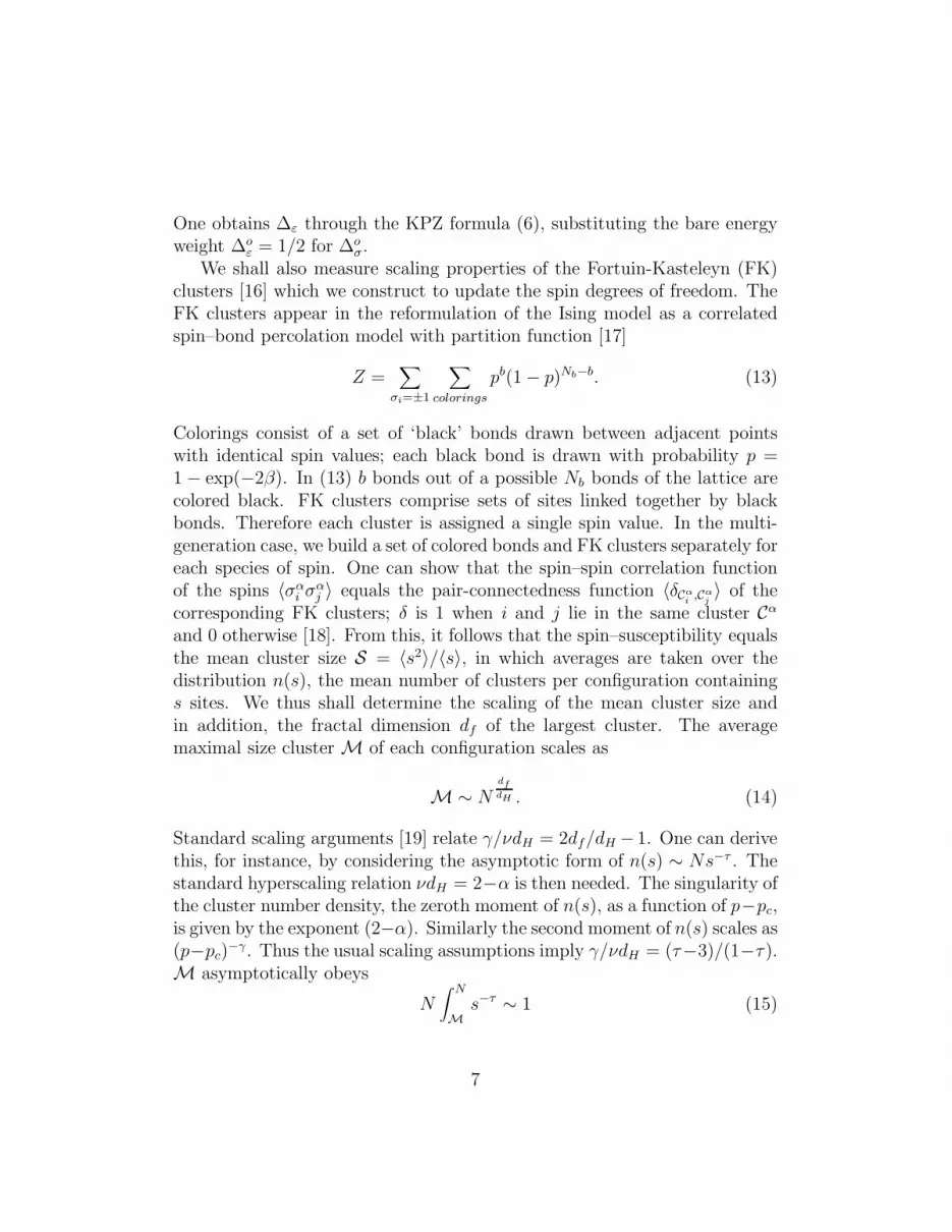
We shall also measure scaling properties of the Fortuin-Kasteleyn (FK)clusters [16] which we construct to update the spin degrees of freedom. TheFK clusters appear in the reformulation of the Ising model as a correlatedspin–bond percolation model with partition function [17]
Z =∑
σi=±1
∑
colorings
pb(1 − p)Nb−b. (13)
Colorings consist of a set of ‘black’ bonds drawn between adjacent pointswith identical spin values; each black bond is drawn with probability p =1 − exp(−2β). In (13) b bonds out of a possible Nb bonds of the lattice arecolored black. FK clusters comprise sets of sites linked together by blackbonds. Therefore each cluster is assigned a single spin value. In the multi-generation case, we build a set of colored bonds and FK clusters separately foreach species of spin. One can show that the spin–spin correlation functionof the spins 〈σα
i σαj 〉 equals the pair-connectedness function 〈δCα
i,Cα
j〉 of the
corresponding FK clusters; δ is 1 when i and j lie in the same cluster Cα
and 0 otherwise [18]. From this, it follows that the spin–susceptibility equalsthe mean cluster size S = 〈s2〉/〈s〉, in which averages are taken over thedistribution n(s), the mean number of clusters per configuration containings sites. We thus shall determine the scaling of the mean cluster size andin addition, the fractal dimension df of the largest cluster. The averagemaximal size cluster M of each configuration scales as
M ∼ Ndf
dH . (14)
Standard scaling arguments [19] relate γ/νdH = 2df/dH − 1. One can derivethis, for instance, by considering the asymptotic form of n(s) ∼ Ns−τ . Thestandard hyperscaling relation νdH = 2−α is then needed. The singularity ofthe cluster number density, the zeroth moment of n(s), as a function of p−pc,is given by the exponent (2−α). Similarly the second moment of n(s) scales as(p−pc)
−γ. Thus the usual scaling assumptions imply γ/νdH = (τ−3)/(1−τ).M asymptotically obeys
N∫ N
M
s−τ ∼ 1 (15)
7

(that is, the mean number of clusters per configuration of size greater thanM is of order unity) and hence df/dH = 1/(τ − 1). Eliminating τ then givesthe above relation between df/dH and γ/νdH .
We can also obtain additional information about the critical geometryof these theories by examining the properties of pure percolation clusters.Consider the bond-percolation model
Z =∑
colorings
pb(1 − p)Nb−bqNc , (16)
which for q = 2 is yet another formulation of the Ising partition functionand more generally is the partition function of the q-state Potts model. Thepair-connectedness function then exhibits the scaling behavior at criticalityof (5) with weights [20]
∆oσ,q = ∆o
σ,q =(1 − y2)
8(2 − y); cos(
πy
2) =
1
2
√q. (17)
The q → 1 limit corresponds to pure percolation, which has no dynamics(and vanishing central charge) and thus does not induce any back-reactionwhen it is coupled to a theory of gravity and matter of central charge c.∆o
σ,q=1 = 5/96; the dressed weight is again governed by the KPZ formula (6).With this new dressed weight, we can then predict the scaling behavior ofthe mean (and maximal) cluster sizes SN,q=1 (and MN,q=1) using (10) withS substituted for χ.
In our simulations, we shall consider site percolation, in which sites(rather than bonds) are colored black with probability p and clusters arebuilt by connecting adjacent colored sites. It is well known that bond andsite percolation are in the same universality class, so that the scaling predic-tions described above should still hold in the case of pure site percolation. Itis advantageous to consider site percolation because the critical value of p,pc, is constrained to equal 1/2 for site-percolation on triangulations [21]2.
2.1 c = 1
The scaling relations become more complicated for c = 1. Analytic solutionsof the c = 1 matrix models (and a careful analysis of Liouville theory) show
2There are some possible exceptions to this constraint, which definitely do not applyin the cases we shall consider here. This issue is discussed extensively in [14].
8

that correlation functions no longer scale simply as powers of the cosmologicalconstant µ. Instead, the appropriate scaling variable is η which satisfies 3
µ = −η ln(η) + c1η + · · · (18)
in the limit of small η; c1 is a constant that we do not specify and shallnot assume to be universal. This scaling relation has been derived for theGaussian theory (of finite and infinite radius) coupled to gravity. The productof Ising models lies on the Gaussian c = 1 orbifold line [22]; coupled to gravity,it is not equivalent to the solved matrix models. We shall assume that theasymptotic logarithmic scaling violation is characteristic of c = 1 and thusholds in the two-species case. Then we conjecture that the scaling relation(7) should be modified so that 4
〈∑
i,j
σαi σα
j 〉(µ)Z(µ) ∼ η(µ)2(−1+∆σ)+(2−γs)(1−h). (19)
In the case of pure percolation, the pair-connectedness function should besubstituted for the spin–spin correlation function, and the dressed Ising
weight ∆σ = 1/4 should be replaced by ∆σ,q=1 =√
5/96. In the follow-ing formulae, χ and the mean cluster size S are interchangeable.
Our simulations will be done on worldsheets of toroidal topology (h = 1)for which Z(µ) ∼ ln(η) for c = 1 (for those models that have been solvedanalytically, so again we are making an assumption about universality). Toextract the asymptotic scaling behavior of χN , we invert the relation betweenη and µ order by order in 1/ lnµ and ln(− ln(µ))/ ln(µ) to obtain
η = − µ
ln µ
1 +ln(− lnµ)
ln µ+
(
ln(− ln µ)
lnµ
)2
− ln(− ln µ)
(lnµ)2+ · · ·
. (20)
We then expand the inverse Laplace transform of (19) to obtain
NχNZN ∼ 1
N(N ln N)ω
1 − ln lnN
ln N+
(
ln ln N
ln N
)2
− ln lnN
(ln N)2+ · · ·
ω
×(
1 +ωΨ(−ω)
ln N− ωΨ(−ω)
ln ln N
(lnN)2+ · · ·
)
;(21)
3 Without loss of generality, we set µc = 0.4The essential role of logarithmic corrections in interpreting numerical measurements
of γs at c = 1 has been previously discussed in reference [23].
9

ω = 2(−1 + ∆σ) = −γ/νdH − 1 (or ω = 2(−1 + ∆σ,q=1) for pure sitepercolation) and Ψ is the digamma function. The scaling behavior of NZN
is obtained by inverse Laplace transforming ∂Z(η(µ))/∂µ:
ZN ∼ 1
N
(
1 +1
ln N− ln ln N
(ln N)2+ · · ·
)
. (22)
In addition to the higher order terms that we have dropped from the inver-sion, there are additional corrections to the above formulae. The correctionthat depends on c1 in (18), which we neglect, should lead to contributionsto (21) and (22) that are competitive with the smallest corrections that wehave included above. In addition, there should be the usual corrections to thescaling (19), but these will be suppressed by powers of 1/N and are negligiblefor moderately large N .
The difference in the theoretically predicted scaling behavior of percola-tion clusters at c = 1, compared to c = 1/2, illustrates the sensitivity of theworldsheet geometry to the presence of the Ising spins. This should induce aneffective coupling between species, which we should be able to detect throughcorrelations between different species’ observables. To look for this coupling,we shall measure
eαβ =1
3N
(
〈EαEβ〉 − 〈Eα〉〈Eβ〉)
(23)
and
mαβ =1
N
(
〈|Mα||Mβ|〉 − 〈|Mα|〉〈|Mβ|〉)
(24)
with Eα =∑
ij Cij(T )σαi σα
j and |Mα| =∑
i |σαi |. A nonzero effective coupling
between species should then be manifest through the quantities e∗ = 2e12/tre and m∗ = 2m12/tr m, which vanish when Eα (|Mα|) are uncorrelated andare 1 or −1 when they are respectively perfectly correlated or anti-correlated.
3 Numerical Simulations and Results
The partition function (1) is evaluated numerically by a Monte Carlo simu-lation. The sum over triangulations is implemented via the standard DTRSalgorithm [24]. This updates the connectivity matrix Cij by flips on ran-domly chosen pairs of triangles sharing a common link. The Ising spins areupdated using the Swendsen-Wang algorithm [25]; one builds FK clusters
10

over the entire lattice and then assigns a randomly chosen value to the spinassociated with each cluster.
Runs were performed on lattices of toroidal topology of size N = 2048, 4096, 8192and 16384. Each sweep consisted of 3N flips of randomly chosen links fol-lowed by a Swendsen-Wang update of the spins. To perform the percolationmeasurements the sites on the lattice were then randomly colored and perco-lation clusters constructed. We used the jacknife technique to estimate ourerrors. We measured auto-correlation functions and computed integratedauto- correlation times, using standard techniques [17]. The magnetization,susceptibility and cluster sizes exhibited considerable critical slowing down5. It was necessary therefore to sample quite a large number of lattices- for each data point between 15, 000 and 30, 000 independent lattices, re-quiring from 30, 000 to 900, 000 sweeps. The total CPU-time used was ap-proximately equivalent to six months on an HP-9000 (720) workstation. Wehistogrammed our data [27]. For cluster data on the larger lattices, how-ever, histogramming was not reliable, given our statistics. The cluster dataexhibited extremely large fluctuations from one measurement to the next;presumably this was the source of the poor performance of histogramming.
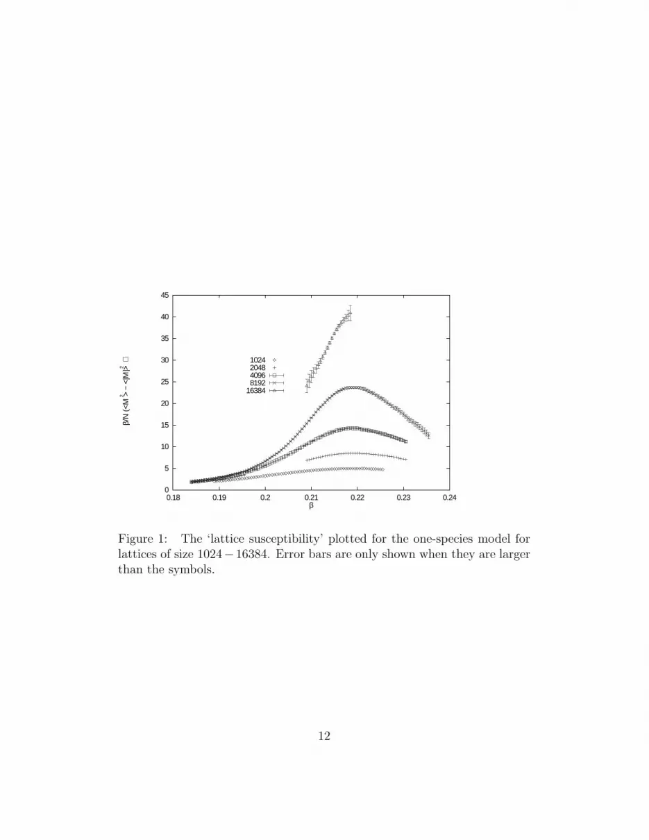
To extract critical exponents using finite-size scaling we must first deter-mine the critical point. We estimated the value of βc by locating the peak inthe lattice susceptibility β/N(〈M2〉−〈|M |〉2), where M is the magnetizationaveraged over species 6. We first present our results for a single species. Fig-ure 1 reveals that this quantity peaks at a value of βc = .2185(20). We alsoplotted Binder’s cumulants [28] UM = 1− 〈M4〉/(3〈M2〉2) as a function of βfor different lattice sizes. From the position of the intersections of these cu-mulants, we estimate βc = .2180(7). The critical temperature for Ising spinson lattices dual to our triangulations was computed analytically in [29], soby the Ising duality relation, it follows that βc = (1/2) ln(131/85) ∼ .216273.Our numerical estimate of the critical value of β is therefore somewhat high.
One could also envision locating the critical temperature by looking for aminimum of the mean pure percolation cluster size as a function of β. Thegrowth in the mean cluster size is determined by the exponent (γ/νdH)q=1,
5More detail on critical slowing down for various algorithms applied to spin models onrandom lattices will appear in future work [26].
6Note that this does not equal the susceptibility χN defined in section (2). χN containsno subtractions and agrees with the continuum susceptibility only in the high-temperaturephase.
11
0
5
10
15
20
25
30
35
40
45
0.18 0.19 0.2 0.21 0.22 0.23 0.24
β/Ν
(<Μ
> −
<|Μ
|> )
2
2
β
1024204840968192
16384
Figure 1: The ‘lattice susceptibility’ plotted for the one-species model forlattices of size 1024−16384. Error bars are only shown when they are largerthan the symbols.
12

0.47
0.48
0.49
0.5
0.51
0.52
0.53
0.54
0.55
0.215 0.216 0.217 0.218 0.219
Bin
der’
s C
umul
ant
β
819240962048819240962048
Figure 2: Binder’s cumulants UM for N = 2048, 4096 and 8192 lattices insimulations of the one species Ising model for lattices of size 1024 − 16384.Lines are drawn to guide the eye.
13

β
Mea
n pe
rcol
atio
n cl
uste
r si
ze f
or N
= 2
048
0.1 0.12 0.14 0.16 0.18 0.2 0.22 0.24320
330
340
350
360
Figure 3: The mean size of percolation clusters as a function of β for theone species Ising model on 2048 node lattices. The dip occurs near criticality.The dotted line is drawn to guide the eye.
which decreases with c. We would therefore expect that percolation clustersfor a given lattice size will become smaller as c increases or likewise as β istuned to bring the Ising spins to criticality. In Fig. 3 we do indeed observea dip in the mean cluster size around the estimated value of βc. The dipis quite broad, however, and doesn’t pinpoint βc; the distinction betweenthe β = .218 and .210 points in the figure may be a statistical artifact.For N = 4096, for instance, with better statistics we find that the meansize is measured to be 571.8 ± 1.9, 571.1 ± 1.9, 573.1 ± 1.9, 572.0 ± 1.8 and572.6±1.9 for β = .211, .213, .215, .216273 and the .218. Thus we observe nosignificant variation over a range δβ = .007. On the other hand the breadth
14

N 1024 2048 4096 8192 theory(γ/νdH)eff from χ .702 (6) .705 (5) .686 (6) .688 (10) 2/3
(γ/νdH)eff from SFK .701 (7) .690 (9) .676 (12) 2/3(df/dH)eff .844 (5) .839 (7) .830 (8) 5/6
(γ/νd)effq=1 .747 (6) .741 (7) .722 (10) .710
(df/dH)effq=1 .866 (5) .866 (6) .852 (8) .855
Table 1: Summary of exponents extracted from finite-size scaling at the exactvalue of βc for one Ising species. The exponents are computed using datafrom lattices of size N and 2N .
of the dip means that measurements of (γ/νdH)q=1 are not very sensitiveto the estimated value of βc. This is not true for the exponent (γ/νdH)which, as we shall see, exhibits a strong dependence on the estimated criticaltemperature.
From the finite-size scaling relation (10) we define the effective exponents
(γ/νdH)eff ≡ ln
(
χ2N
χN
)
/ ln 2. (25)
When cluster sizes rather than the spin–susceptibility are considered, it isimplicit that S is to be substituted for χ in the above definition. Likewise,
(df/dH)eff ≡ ln(M2N
MN
)
/ ln 2. (26)
As usual, the analogous exponents for pure percolation are defined as abovewith subscript q = 1. We now summarize our results for these critical expo-nents, extracted through finite size scaling of χN , the mean FK cluster sizeSFK , the maximal FK cluster size MFK, the mean percolation cluster sizeSq=1 and the maximal percolation cluster size Mq=1. In table (1), we presentthese values obtained from runs at the known value of βc ∼ .216273. The
exact values are γ/νdH = 2/3, df/dH = 5/6, (γ/νdH)q=1 = (4−√
7/2)/3 and
(df/dH)q=1 = (7−√
7/2)/6. The agreement between our measurements and
the theoretical predictions is quite good. Since (df/dH) only describes prop-erties of the largest cluster, it might be less subject to corrections to scaling(for small cluster sizes) and thus provide the best estimator of the critical
15
N 1024 2048 4096 8192 theory(γ/νdH)eff from χ .74 (3) .76 (3) .73 (2) .76 (4) 2/3
(γ/νdH)eff from SFK .748 (14) .741 (8) 2/3(df/dH)eff .877 (15) .869 (6) 5/6
(γ/νd)eff,q=1 .750 (10) .739 (8) .710(df/dH)eff,q=1 .871 (7) .867 (5) .855
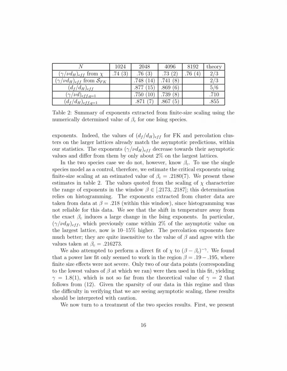
Table 2: Summary of exponents extracted from finite-size scaling using thenumerically determined value of βc for one Ising species.
exponents. Indeed, the values of (df/dH)eff for FK and percolation clus-ters on the larger lattices already match the asymptotic predictions, withinour statistics. The exponents (γ/νdH)eff decrease towards their asymptoticvalues and differ from them by only about 2% on the largest lattices.
In the two species case we do not, however, know βc. To use the singlespecies model as a control, therefore, we estimate the critical exponents usingfinite-size scaling at an estimated value of βc = .2180(7). We present theseestimates in table 2. The values quoted from the scaling of χ characterizethe range of exponents in the window β ∈ [.2173, .2187]; this determinationrelies on histogramming. The exponents extracted from cluster data aretaken from data at β = .218 (within this window), since histogramming wasnot reliable for this data. We see that the shift in temperature away fromthe exact βc induces a large change in the Ising exponents. In particular,(γ/νdH)eff , which previously came within 2% of the asymptotic value onthe largest lattice, now is 10–15% higher. The percolation exponents faremuch better; they are quite insensitive to the value of β and agree with thevalues taken at βc = .216273.
We also attempted to perform a direct fit of χ to (β − βc)−γ . We found
that a power law fit only seemed to work in the region β = .19− .195, wherefinite size effects were not severe. Only two of our data points (correspondingto the lowest values of β at which we ran) were then used in this fit, yieldingγ = 1.8(1), which is not so far from the theoretical value of γ = 2 thatfollows from (12). Given the sparsity of our data in this regime and thusthe difficulty in verifying that we are seeing asymptotic scaling, these resultsshould be interpreted with caution.
We now turn to a treatment of the two species results. First, we present
16

0
5
10
15
20
25
30
35
40
45
0.18 0.19 0.2 0.21 0.22 0.23 0.24
β/Ν
(<Μ
> −
<|Μ
|> )
2
2
β
1024204840968192
16384
Figure 4: A plot of the ‘lattice susceptibility’ for the two species case withN = 2048, 4096, 8192 and 16384. Error bars are only shown when they arelarger than the symbols.
plots of β/N(〈M2〉 − 〈|M |〉2) and the intersections of Binder’s cumulants.Note that these observables look qualitatively very similar to their one
species counterparts. The position of the susceptibility peak is β = .2185+35−20.
The Binder’s cumulants (taken from the largest lattices where we have suffi-cient data to determine intersections) give βc = .217(1). As in the one-speciescase we adopt the Binder’s estimate, which seems to be more precise. Basedon the logarithmic corrections to scaling discussed in section 2, we would es-timate that on the lattice sizes simulated we are further from the asymptoticscaling regime than in the one species case. It is therefore likely that ourestimate of βc here is less precise.
In table 3, we compare the finite-size scaling measurements of (γ/νdH)eff
and (γ/νdH)effq=1 with the theoretical exponents, computed from the KPZ for-
mula, neglecting logarithmic corrections. The first row contains an estimateof the susceptibility exponent based on histogram extrapolations within theregion β = .216 to .218. We observed that measuring the mean-size of FK
17

0.575
0.58
0.585
0.59
0.595
0.6
0.605
0.61
0.215 0.216 0.217 0.218 0.219
Bin
der’
s C
umul
ant
β
8192409681924096
Figure 5: Binder’s cumulants for N = 4096 and N = 8192 as measured inthe two species model.
1024 2048 4096 8192 theory(γ/νd)eff from χ .73 (3) .73 (3) .75 (5) .74 (4) 1/2
(γ/νd)eff,q=1 .759 (11) .717 (5) .712 (7) .709 (10) .544(df/dH)eff,q=1 .852 (6) .848 (4) .848 (5) .848 (6) .772
(γ/νd)eff,q=1(X) .739 (7) .732 (7) .700 (10) .544(df/dH)eff,q=1(X) .861 (5) .859 (7) .841 (8) .772
Table 3: Summary of exponents extracted from finite-size scaling for two Isingspecies compared with KPZ exponents, without logarithmic corrections. Inthe last two rows, we present the corresponding percolation exponents forlattices on which a Gaussian field X was simulated.
18

clusters (at β = .216) always yielded exponents agreeing with those extractedfrom the spin–susceptibility. Since the cluster data did not histogram reliably,it was difficult though to estimate the corresponding exponents throughoutthe above range of β without taking a large amount of additional data. FKcluster scaling was primarily measured just to verify that it agreed with thescaling of the spin–susceptibility. Our data already showed this, so it didnot seem worthwhile to repeat runs to measure the cluster scaling at varioustemperatures. The following rows thus summarize data for pure percolationclusters, which was relatively insensitive to β; i.e. a shift of β of .005 didnot induce a stastically significant change in the q = 1 exponents. Sinceagain percolation cluster data did not histogram reliably, we present datataken at β = .216 in table 3; these should be representative of the values onewould measure throughout the region β ∈ [.216, .218]. The final two rowsinclude exponents extracted from simulations of a Gaussian field X coupledto gravity, as discussed in [14].
What is most striking about the measured c = 1 exponents is in factthat they agree quite well with the c = 1/2 data (taken from the numericallyestimated range of βc) and in the case of percolation, the c = 1/2 theoreticalpredictions. There is clearly, however, a very large discrepancy between themeasured and theoretical c = 1 scaling exponents. On the larger lattices, thepercolation exponents for the two species Ising model also agree fairly wellwith those measured in the Gaussian field simulations, suggesting some de-gree of universality at c = 1 in their behavior. From equations (21) and (22),we can determine the logarithmic corrections to the exponents (γ/νdH)eff
and (γ/νdH)effq=1. One can easily see that these are considerable by including
the leading correction, which gives
(γ/νdH)eff = γ/νdH +1 + γ/νdH
ln N+ · · · ; (27)
this formula of course holds for q = 1. In Fig. 6 we compare the measured(γ/νdH)eff with the corresponding theoretical predictions including both theleading correction (27) and all of the logarithmic corrections that follow fromequations (21) and (22). The data does not agree particularly well with any ofthe predictions, but that is to be expected, since our estimate of βc most likelyinduces a large error. Note that the theoretical curve including logs lies veryclose to the c = 1/2 asymptotic value of γ/νdH = 2/3 for the lattice sizes wesimulate. The measured values of this exponent for c = 1 and c = 1/2 (when
19

Lattice size N for N to 2N extrapolation
(γ /
ν dH) e
ff f
or K
PZ w
ith lo
g sc
alin
g (c
= 1
)
0 2000 4000 6000 80000.45
0.55
0.65
0.75
0.85
Figure 6: A comparison of the theoretical prediction of the finite–size c =1 magnetic susceptibility scaling with our data. The dotted line includesthe leading logarithmic correction and the solid line takes into account allsubleading terms that we calculated. The horizontal dashed line representsthe prediction without logarithmic corrections.
20

we use the numerically estimated values of βc) are essentially identical, sothat the discrepancy between the theoretical predictions (incorporating logsin the c = 1 case) and the data are thus roughly the same for c = 1 andc = 1/2.
In Fig. 7 a similar comparison is shown for the exponent (γ/νdH)effq=1. We
see that the data and theoretical predictions match quite well. Presumably,as in the c = 1/2 case, the comparison works because this exponent no longerdepends sensitively on our determination of βc. The agreement with theory isabout as successful as in the Gaussian case [14]. This suggests the likelihoodthat at least the leading logarithmic corrections to scaling (27) are correctand universal for c = 1. We should note here that although the data can befit by including the above logarithmic corrections it would not be possible toextract these corrections from the data itself without theoretical guidance.
As in the one species case, we also fitted our lowest β data points toχ ∼ (β − βc)
−γ. The fit yielded γ = 2.03(4) which does not match thetheoretical value of γ = 1 + 1/
√2 ∼ 1.71. It is not clear that this fit is
reliable; probably the exact relation between χ and β should also includelogarithmic corrections.
We finally turn to an examination of correlations (defined in (24) and(23)) between the different spin species. Fig. 8 exhibits definite, thoughmoderately small, correlations between the spins of different species. Asevident in Fig. 9, the correlations between the average species’ energies, asmeasured by e∗, are much smaller. The magnetization (and more directly,the susceptibility) is strongly correlated with the distribution of FK clustersizes, which in turn should be sensitive to the bottlenecks which characterizethe worldsheet geometry. Since the correlations between species are mediatedby fluctuations in the geometry, it is not surprising that they are stronger inthe magnetic sector than in the energy sector. In both cases the correlationsare not so strong, indicating that the Ising spins are only weakly coupling togravity for the lattice sizes we consider.
4 Discussion
To gauge our prospects for extending this work to c > 1, we shall nowattempt to shed more light on the origin of the corrections to scaling atc = 1. The dynamics at c = 1 is governed by the tachyon (the lowest mass
21

Lattice size N for N to 2N extrapolation
(γ /
ν dH) q
= 1
eff
for
KPZ
with
log
scal
ing
(c=
1)
0 2000 4000 6000 80000.5
0.6
0.7
0.8
Figure 7: A comparison of the theoretical prediction of the finite size c = 1scaling of (γ/νdH)q=1 with our percolation data for the two species Isingmodel. The dotted line includes the leading logarithmic correction and thesolid line takes into account all subleading terms that we calculated. Thehorizontal dashed line indicates where these curves asymptote.
22

0
0.05
0.1
0.15
0.2
0.214 0.216 0.218 0.22 0.222
m*
β
8192
Figure 8: The correlation m∗ plotted for the two species model on N = 8192lattices. Recall that the correlations are normalized so that m∗ equals onewhen |Mα=1| and |Mα=2| are fully correlated.
23

0
0.001
0.002
0.003
0.004
0.005
0.215 0.216 0.217 0.218 0.219 0.22
e*
β
8192
Figure 9: The correlation e∗ between the energies of different species plottedfor the c = 1 model on N = 8192 lattices.
operator) which acquires a continuous spectrum with vanishing energy at 0momentum. The scaling corrections arise from the infrared cutoff on thetachyonic momentum, p > 1/ lnN [13]. The origin of this logarithmic cutoffmay not be so evident in the context of the two-species Ising model, sincethe tachyon cannot be expressed so simply in terms of the Ising spins. Thepresence of logarithmic corrections appears to only depend on the value ofthe central charge, so we appeal to universality and consider instead the c = 1Gaussian theory. The tachyon can then be written in terms of the Gaussianfield X as
T (p) ∼∫
√
|g| exp(ipX + (|p| − 2)φ); (28)
φ is the Liouville field and g is the reference metric (g = g exp(−φ)). Theinfrared target space momentum cutoff is then just a consequence of theinfinite Hausdorff dimension of the embedding space [30],
〈XX〉 ∼ (ln N)2. (29)
The suppression of tachyon propagation by finite-size effects effectively weak-ens the coupling between gravity and the Ising spins. Therefore, the spins
24

of each species are only very weakly coupled, and the two and one speciesmodels appear to be qualitatively very similar on the lattices we consider.This should not be true in the continuum limit. We see that without anunderstanding of the corrections to scaling for c = 1, the numerical observa-tions seem to conflict with our theoretical expectations of the onset of strongcoupling at c = 1.
The target space Hausdorff dimension, as measured for Gaussian embed-dings of d somewhat greater than 1, is also large. Thus we would expectthat for c > 1, the tachyon ground state energy still acquires a considerableshift and we expect large corrections to scaling. At c = 1, we were ableto determine these corrections because the c = 1 model is solvable. With-out new theoretical input, the prognosis for understanding simulations for csomewhat greater than 1 thus seems poor.
25

5 Acknowledgments
This work has been done with NPAC (Northeast Parallel Architectures Cen-ter) computing facilities. We would like to thank John Apostolakis, SimonCatterall and Paul Coddington for helpful correspondence and conversations.The research of MB was supported by the Department of Energy OutstandingJunior Investigator Grant DOE DE-FG02-85ER40231, that of MF by fundsfrom NPAC and that of GH by research funds from Syracuse University.
26

References
[1] P. Di Francesco, P. Ginsparg and J. Zinn-Justin, 2D Gravity and Ran-dom Matrices, hep-th/9306153, to appear in Phys. Rep.
[2] V. G. Knizhnik, A. M. Polyakov and A. B. Zamolodchikov, Mod. Phys.Lett. A3 (1988) 819.
[3] D. Kutasov and N. Seiberg, Nucl. Phys. B358 (1991) 600.
[4] G. Moore and P. Ginsparg, Lectures on 2-D Gravity and 2-D StringTheory, TASI Lectures, Yale preprint YCTP-P23-92 and Los Alamospreprint LA-UR-92-3479 (1993), hep-th/9304011.
[5] V. A. Kazakov, Phys. Lett. A119 (1986) 140.
[6] D. V. Boulatov and V. A. Kazakov, Phys. Lett. B186 (1987) 379.
[7] E. Brezin and S. Hikami, Phys. Lett. B283 (1992) 203.
[8] S. Hikami and E. Brezin, Phys. Lett. B295 (1992) 209.
[9] S. Hikami, Phys. Lett. B305 (1993) 327.
[10] C. Baillie and D. Johnston, Mod. Phys. Lett. A7 (1992) 1519; Phys.Lett. B286 (1992) 44.
[11] S. M. Catterall, J. B. Kogut and R. L. Renken, Phys. Rev. D45 (1992)2957; Phys. Lett. B292 (1992) 277.
[12] J. Ambjørn, B. Durhuus, T. Jonsson and G. Thorleifsson, Nucl. Phys.B398 (1993) 568.
[13] I. Klebanov, String Theory in Two-Dimensions, in Proc. of the TriesteSchool on String Theory and Quantum Gravity ’91 (hep-th/9108019).
[14] Geoffrey Harris, Percolation on Strings and the Cover-up of the c=1Disaster, Syracuse University preprint SU-HEP 4241-555.
[15] F. David, Mod. Phys. Lett. A3 (1988) 1651; J. Distler and H. Kawai,Nucl. Phys. B321 (1989) 509.
27

[16] C. M. Fortuin and P. W. Kasteleyn, Physica 57 (1972) 536.
[17] A. Sokal, Monte Carlo Methods in Statistical Mechanics: Foundationsand Algorithms, NYU preprint based on lectures at the Troisieme Cyclede la Physique en Suisse Romande, June 1989.
[18] C.-K. Hu, Phys. Rev. B29 (1984) 5103.
[19] D. Stauffer and A. Aharony, Introduction to Percolation Theory (Taylorand Francis, London, U.K. 1992).
[20] M. den Nijs, Phys. Rev. B27 (1983) 1674.
[21] M. F. Sykes and J. W. Essam, J. Math. Phys. 5 (1964) 1117.
[22] P. Ginsparg, in Fields, Strings and Critical Phenomena, Les HouchesProceedings, Vol. 49, ed. E. Brezin and J. Zinn-Justin (North Holland,Amsterdam 1983) 5.
[23] J. Ambjørn, D. Boulatov and V. A. Kazakov, Mod. Phys. Lett. A5(1990) 771.
[24] D. Boulatov, V. Kazakov, I. Kostov and A. A. Migdal, Phys. Lett. B157(1985) 295.
[25] R.H. Swendsen and J.-S. Wang, Phys. Rev. Lett. 58 (1987) 86.
[26] M. Bowick, M. Falcioni, G. Harris and E. Marinari, Phys. Lett. B322(1994) 316.
[27] M. Falcioni, E. Marinari, M. L. Paciello, G. Parisi and B. Taglienti,Phys. Lett. 102B (1981) 270; A. M. Ferrenberg and R. H. Swendsen,Phys. Rev. Lett. 61 (1988) 2635; and Erratum, ibidem 63 (1989) 1658.
[28] K. Binder, Z. Phys. B43 (1981) 119.
[29] Z. Burda and J. Jurkiewicz, Acta Physica Polonica B20 (1989) 949.
[30] V. A. Kazakov and A. A. Migdal, Nucl. Phys. B311 (1988) 171.
28


