Embed Size (px)
Citation preview

Chapter 1
Two-Dimensional QuantumGravity
Ivan Kostov
Institut de Physique Theorique CEA Saclay,
F-91191 Gif-sur-Yvette Cedex, France
Abstract
This chapter contains a short review the correspondence between large N matrix
models and critical phenomena on lattices with fluctuating geometry.
1.1 Introduction
One of the applications of the large N matrix models is that they can be used as
machines for generating planar graphs. The problem of counting planar graphs
was related to the saddle point solution of matrix integrals by Brezin, Parisi,
Itzykson and Zuber [BIPZ78]. The concept of the 1/N expansion for matrix
fields and its topological meaning was introduced by ’t Hooft in [tH74].
The ensembles of planar graphs exhibit universal critical behavior. By tun-
ing the coupling constants one can achieve a regime which is dominated by
planar graphs of diverging size. Seen from a distance, such planar graphs re-
semble surfaces with fluctuating metric. Therefore the sum over planar graphs
can be considered as a discretization of the path integral of 2d quantum gravity
[Pol81]. The interpretation of the ensembles of planar graphs as models of 2D
lattice gravity was suggested in [Dav85b, Kaz85, ADF85] and further studied
in [Dav85a, KKM85, BKKM86].
The 2d lattice gravity with matter fields was initially constructed as a
gaussian discretization of the path integral for the non-critical Polyakov string
[Pol81] with D-dimensional target space. However such a discretization leads

2 CHAPTER 1. AKEMANN ET AL.
to an exactly solvable model only in the case of D = 0 and D = −2 [KKM85,
BKKM86, KM87]. Another way to introduce a non-trivial target space is to
consider solvable spin models on planar graphs. The Ising model on a dy-
namical lattice was solved, after being reformulated as a two-matrix model, by
Kazakov and Boulatov [Kaz86, BK87]. This solution was used as a guideline
by Knizhnik, Polyakov and Zamolodchikov, who obtained the exact spectrum
of anomalous dimensions in the continuum theory of 2d gravity [KPZ88].
Soon after the the Ising model, all basic statistical models were solved on a
dynamical lattice: the O(n) model [Kos89a], the Q-state Potts model [Kaz88],
the SOS and ADE height models [Kos89b][Kos92b], as well as the 6-vertex
model [Kos00]. Particular cases of the Potts and O(n) models are the tree/bond
percolation [Kaz88] and self-avoiding polymer networks [DK88] [DK90]. In
general, the theories of discrete gravity admit an infinite number of multi-
critical regimes, which are first observed in the one-matrix model [Kaz89]. The
multi-critical point in the ADS models and the O(n) model were identified in
[Kos92b, KS92].
Practically all solvable 2d statistical models whose critical behaviour is de-
scribed by a c 6 1 CFT can be transfered from the plane to a dynamical lattice
and solved exactly. There can be several different discretizations of the same
continuous theory. For example, all rational theories of 2D gravity can be ob-
tained either by the ADE matric models, or as the critical points of the 2-matrix
model [DKK93].
For statistical systems coupled to gravity it is possible to solve analytically
problems whose exact solution is inaccessible on flat lattice. On the other hand,
the solution of a spin model on a dynamical lattice allows to reconstruct the
phase diagram and the critical exponents of the same spin model on the flat
lattice. Therefore the solvable models of 2d gravity represent a valuable tool
to explore the critical phenomena in two dimensions. This is especially true in
presence of boundaries, where the solution of the matrix model can give insight
about the interplay between the bulk and the boundary flows.
We review the solvable models of 2d lattice quantum gravity and the way
they are related to matrix models. We put the accent on the critical behavior
and the solution in the scaling limit near the critical points. We start with a
short description of the continuum world sheet theory, the Liouville gravity, and
derive the KPS scaling relation. Then we present in detail the simplest model
of 2d gravity and the corresponding matrix model, followed by less or more
sketchy presentation of the vertex/height integrable models on planar graphs
and their mapping to matrix models.

1.2. LIOUVILLE GRAVITY AND KPZ SCALING RELATION 3
1.2 Liouville gravity and KPZ scaling relation
The continuum approach to critical phenomena in presence of gravity was de-
velopped by Knizhnik, Polyakov and Zamolodchikov [KPZ88]. The confor-
mal weights from the Kac spectrum are converted by ‘gravitational dressing’
into new ones through the remarkable KPZ formula [KPZ88]. Subsequently,
a more intuitive alternative derivation of the KPZ formula was proposed in
[Dav88, DK89]. The conformal theory with quantum gravity has larger sym-
metry and hence simpler phenomenology: we are allowed to ask only questions
invariant under diffeomorphisms. The anomalous dimensions in such a theory
are perfectly meaningful but not the operator product expansion; only fields
integrated over all points make sense. Therefore, instead of the correlation
functions of the local operators we have to consider the corresponding suscepti-
bilites. The way they depend on the temperature and the cosmological constant
allows to determine the scaling dimensions.
1.2.1 Path integral over metrics
Let Zmatter[gab] be the partition function of the matter field on a two-dimensional
worldsheet M with Riemann metric gab. For the moment assume that the world
sheet is homeomorphic to a sphere. The partition function on the sphere, which
we denote by F(µ), is symbolically written as the functional integral
F(µ) =
∫
[Dgab] e−µA Z(sphere)
matter [gab], (1.2.1)
where the parameter µ, called cosmological constant, is coupled to the area of
the worldsheet,
A =
∫
Md2σ
√
det gab. (1.2.2)
For a worldsheet M with a boundary ∂M one can introduce a second pa-
rameter, the boundary cosmological constant µB coupled to the boundary length
ℓ =
∫
∂M
√
gab dσadσb . (1.2.3)
The partition function on the disk, which we denote by U(µ, µB), is defined as
a functional integral over all Riemann metrics on the disk,
U(µ, µB) =
∫
[Dgab] e−µA−µBℓ Z(disk)
matter[gab]. (1.2.4)
Here we assumed that the matter field satisfy certain boundary condition. We
will also consider more complicated situations where the boundary is split into

4 CHAPTER 1. AKEMANN ET AL.
several segments with different boundary cosmological constants and different
boundary conditions for the matter field.
By the invariance of the functional measure under diffeomorphisms of the
world sheet one can impose the conformal gauge
gab = e2φ gab, (1.2.5)
where gab is some background metric, so that the fluctuations of the metric
are described by the local scale factor φ. At the critical points, where the
matter QFT is conformal invariant, the scale factor φ couples to the matter
field through a universal classical action induced by the conformal anomaly
cmatter. In addition, the conformal gauge necessarily introduces the Faddeev-
Popov reparametrization ghosts with central charge cghosts = −26 [Pol81] . The
effective action of the field φ is called Liouville action because the correspond-
ing classical equation of motion is the equation for the metrics with constant
curvature, the Liouville equation.
1.2.2 Liouville gravity
Liouville gravity is a term for the two-dimensional quantum gravity whose ac-
tion is induced by a conformal invariant matter field. The effective action of the
Liouville gravity consists of three pieces, associated with the matter, Liouville
and ghost fields. For our discussion we will only need the explicit form of the
Liouville piece Aµ,µB[φ]. This is the action of a gaussian field with linear cou-
pling to the curvature and exponential terms coupled to the bulk and boundary
cosmological constants:
Aµ,µB[φ] =
1
4π
∫
M
(
g (∇φ)2 + QφR)
+1
2π
∫
∂M
dσQφK
+µA + µBℓ. (1.2.6)
The area and the length are defined by (1.2.2) and (1.2.3), R the background
curvature in the bulk and by K the geodesic background curvature at the
boundary. The coupling to the curvature is through the imaginary background
charge iQ. We will assume that the coupling constant g of the Liouville field is
larger than one: g ≥ 1.
The Liouville coupling g and the background charge Q are determined by
the invariance with respect to the choice of the background metric gab. The
background charge of the Liouville field must be tuned so that the total con-
formal anomaly vanishes:
ctot ≡ cφ + cmatter + cghosts
= (1 + 6Q2/g) + cmatter − 26 = 0. (1.2.7)

1.2. LIOUVILLE GRAVITY AND KPZ SCALING RELATION 5
The ballance of the central charge gives
cmatter = 1 − 6(g − 1)2/g. (1.2.8)
The observables in Liouville gravity are integrated local densities
O ∼∫
MΦh e2αφ , (1.2.9)
where Φh represents a scalar (h = h) matter field1 and Vα is a Liouville ‘dressing’
field, which completes the conformal weights of the matter field to (1, 1). The
balance of the conformal dimensions, h + hLiouvα = 1, gives a quadratic relation
between the Liouville dressing charge and the conformal weight of the matter
field:
h +α(Q − α)
g= 1 . (1.2.10)
In particular, the Liouville interaction e2φ dresses the identity operator. The
balance of scaling dimensions (1.2.10) determines, for α = 1 and h = 0, the
value of the background charge Q:
Q = g + 1. (1.2.11)
Similarly, the boundary matter fields ΦBh with boundary dimensions hB are
dressed by boundary Liouville exponential fields,
OB ∼∫
∂MΦB
h eαBφ , (1.2.12)
where the boundary Liouville exponent αB is related to h as in (1.2.10).
The quadratic relation (1.2.10) has two solutions, α and α, such that α ≤Q/2 and α ≥ Q/2. The Liouville dressing fields corresponding to the two
solutions are related by Liouville reflection α → α = Q − α. Generically the
scaling limit of the operators on the lattice is described by smaller of the two
solutions of the quadratic constraint (1.2.10). The corresponding field Vα has
a good quasiclassical limit. Such fields are said to satisfy the Seiberg bound
α 6 Q/2, see the reviews [DFGZJ95, GM93].2
The simplest correlation functions in Liouville gravity (up to 3-point func-
tions of the bulk fields and 2-point functions of the boundary fields) factorize
into matter and Liouville pieces. This factorization does not hold away from
the critical points.
1The fields cannot have spin because any local rotation can be ‘unwound’ by a coordinatetransformation.
2Originally it was believed that the second solution is unphysical, until it was realized thatit describes specially tuned measure over surfaces [Kle95].

6 CHAPTER 1. AKEMANN ET AL.
1.2.3 Correlation functions and KPZ scaling relation
The scaling of the correlation function with the bulk cosmological constant
µ follows from the covariance of the Liouville action (1.2.6) with respect to
translations of the Liouville field:
Aµ,µB[φ − 1
2 ln µ] = −12Qχ ln µ + A1, µB/
√µ[φ ] (1.2.13)
where χ = 2− 2#(handles) − #(boundaries) is the Euler characteristics of the
worldsheet. Applying this to the correlation function of the bulk operators Oj
and the boundary operators OBk , we obtain the scaling relation
⟨
∏
j
Oj
∏
k
OBk
⟩
µ,µB
= µ12χQ−
P
j αj− 12
P
k αBk f(µB/
õ), (1.2.14)
where f is some scaling function. We see that for any choice of the local fields
the unnormalized correlation function dependence on the global curvature of the
world sheet through an universal exponent Q = 1+g = 2−γstr, where γstr = 1−g
is called string susceptibility exponent. The scaling of the bulk and boundary
local fields are determined by their gravitational anomalous dimensions ∆i and
∆Bj , related to the exponents αi and αB
j by
∆i = 1 − αi, ∆Bi = 1 − αB
i . (1.2.15)
Once the exponent γstr and the gravitational dimensions ∆i are known,
the central charge cmatter and conformal weights hi of the matter fields can be
determined from (1.2.7) and (1.2.10):
h =∆(∆ − γstr)
1 − γstr, cmatter = 1 − 6
γ2str
1 − γstr(γstr = 1 − g), (1.2.16)
and a similar relation for the boundary fields. This relation is known as KPZ
correspondence between flat and gravitational dimensions of the local fields
[KPZ88, Dav88, DK89].
The ‘physical’ solution of the quadratic equation (1.2.10) can be parametrized
by a pair of real numbers r and s, not necessarily integers,3
hrs(g) =(rg − s)2 − (g − 1)2
4g, αrs(g) =
g + 1 − |rg − s|2
. (1.2.17)
The corresponding gravitational anomalous dimension ∆rs = 1 − αrs are
∆rs(g) =|rg − s| − (g − 1)
2. (1.2.18)
3When r and s are integers, hrs are the conformal weights of the the degenerate fields ofthe matter CFT.

1.3. DISCRETIZATION OF THE PATH INTEGRAL OVER METRICS 7
We remind that our conventions are such that g > 1. The solution (1.2.17)
apply also for the boundary exponents, after replacing h → hB ,∆ → ∆B , α →β. It generalizes in obvious way to the case when each boundary segment is
characterized by a different boundary cosmological constant.
The string susceptibility exponent γstr is a measurable quantity in the dis-
crete models of 2D gravity and is determined by the the scaling behavior of the
susceptibility on the sphere u ≡ ∂2µF ∼ µ−γstr at the critical points. At different
critical points of the same model one can have different exponents γstr. Once
γstr is known, the matter central charge and the conformal weights of the local
fields can be determined by the KPZ relation (1.2.16), with the gravitational
demensions ∆i and ∆Bi defined through the scaling relation
⟨
∏
j
Oj
∏
k
OBk
⟩
µ,µB
= µ12χ(2−γstr)−
P
j(1−∆i)− 12
P
k(1−∆Bk
) f(µB/√
µ). (1.2.19)
1.3 Discretization of the path integral over metrics
The statement that the integral over Riemann metrics can be discretized by the
sum over a sufficiently large ensemble of planar graphs has no rigorous proof,
but it has passed a multitude of quantitative tests. In order to built models of
discrete 2D gravity it is sufficient to consider the ensemble of trivalent planar
graphs which are dual to triangulations, as the one shown in Fig. 1.1. To avoid
ambiguity the propagators are represented by double lines. The faces of such a
‘fat’ graph are bounded by the polygons formed by the single lines.
1/β
i ij
j
k
k
ij
ij
β
Figure 1.1: Left: A trivalent planar graph with the topology of a disk and its dultriangulation. Right: Feynman rules for the matrix model for pure gravity.
The local curvature of the triangulation is concentrated at the vertices r
of the triangulation. The curvature Rr (or the boundary curvature Kr if the
vertex is on the boundary) is expressed through the coordination number cr,
equal to the number of triangles meeting at the point r,
Rr = π6 − cr
3, Kr = π
3 − cr
3. (1.3.1)

8 CHAPTER 1. AKEMANN ET AL.
The total curvature is equal to the Euler number χ(Γ):
1
2π
∑
r∈bulk
Rr +1
π
∑
r∈boundary
Kr = χ(Γ) . (1.3.2)
For each fat graph Γ we define the area and the boundary length as
|Γ| def= # (faces of Γ) , |∂Γ| def
= # (external lines of Γ) . (1.3.3)
Let us denote by {Sphere} and {Disk} the ensembles of fat graphs dual
to triangulations respectively of the sphere and of the disk. Assume that the
matter field can be defined on any triangulation Γ and denote its partition
function by Zmatter[Γ]. Then the path integrals for the partition function of the
sphere (1.2.1) and that of the disk (1.2.4) are discretized as follows:
F(µ) =∑
Γ∈{Sphere}
1
k(Γ)µ−|Γ| Z
(sphere)
matter [Γ]. (1.3.4)
U(µ, µB) =∑
Γ∈{Disk}
1
|∂Γ| µ−|Γ| µ−|∂Γ|B Z
(disk)
matter[Γ]. (1.3.5)
Here µ and µB are the the lattice bulk and boundary cosmological constants
and k(Γ) is the volume of the symmetry group of the planar graph Γ.
1.4 Pure lattice gravity and the one-matrix model
1.4.1 The matrix model as a generator of planar graphs
The solution of pure discrete gravity thus boils down to the problem of counting
planar graphs, reformulated in terms of a matrix integral in [BIPZ78]. The
matrix integral
Z(N,β) =
∫
dM eβ
“
−12TrM2+ 1
3TrM3
”
, (1.4.6)
where dM is the flat measure in the linear space of N ×N hermitian matrices,
can be considered as the partition function of a zero-dimensional QFT with
Feynman rules given in Fig. 1.1 (right). The integral is divergent but makes
sense as perturbative expansion around the gaussian measure. The logarithm of
the partition function (1.4.6), the ‘vacuum energy’ of the matrix field, is equal
to the sum of all connected diagrams.
The weight of a vacuum graph Γ is written, using the Euler relation, as
Weight(Γ) =1
k(Γ)β#vertices−#linesN#faces =
1
k(Γ)βχ(Γ) (N/β)|Γ|. (1.4.7)
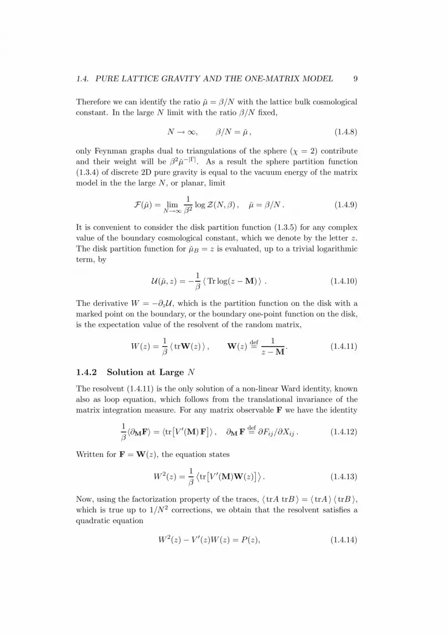
1.4. PURE LATTICE GRAVITY AND THE ONE-MATRIX MODEL 9
Therefore we can identify the ratio µ = β/N with the lattice bulk cosmological
constant. In the large N limit with the ratio β/N fixed,
N → ∞, β/N = µ , (1.4.8)
only Feynman graphs dual to triangulations of the sphere (χ = 2) contribute
and their weight will be β2µ−|Γ|. As a result the sphere partition function
(1.3.4) of discrete 2D pure gravity is equal to the vacuum energy of the matrix
model in the the large N , or planar, limit
F(µ) = limN→∞
1
β2logZ(N,β) , µ = β/N . (1.4.9)
It is convenient to consider the disk partition function (1.3.5) for any complex
value of the boundary cosmological constant, which we denote by the letter z.
The disk partition function for µB = z is evaluated, up to a trivial logarithmic
term, by
U(µ, z) = − 1
β〈Tr log(z − M) 〉 . (1.4.10)
The derivative W = −∂zU , which is the partition function on the disk with a
marked point on the boundary, or the boundary one-point function on the disk,
is the expectation value of the resolvent of the random matrix,
W (z) =1
β〈 trW(z) 〉 , W(z)
def=
1
z − M. (1.4.11)
1.4.2 Solution at Large N
The resolvent (1.4.11) is the only solution of a non-linear Ward identity, known
also as loop equation, which follows from the translational invariance of the
matrix integration measure. For any matrix observable F we have the identity
1
β〈∂MF〉 = 〈tr
[
V ′(M)F]
〉 , ∂M Fdef= ∂Fij/∂Xij . (1.4.12)
Written for F = W(z), the equation states
W 2(z) =1
β
⟨
tr[
V ′(M)W(z)]⟩
. (1.4.13)
Now, using the factorization property of the traces, 〈 trA trB 〉 = 〈 trA 〉 〈 trB 〉,which is true up to 1/N2 corrections, we obtain that the resolvent satisfies a
quadratic equation
W 2(z) − V ′(z)W (z) = P (z), (1.4.14)

10 CHAPTER 1. AKEMANN ET AL.
where P is a polynomial. Therefore the function
J(z)def= W (z) − 1
2V ′(z), (1.4.15)
should be such that that J2(z) is a polynomial. The polynomial is determined
by the asymptotics at infinity,
J(z) = −12V ′(z) + (µz)−1 + O(z−2). (1.4.16)
The solution is
J(z) = (z − 1 + 12(a + b))
√
(z − a)(z − b), (1.4.17)
where the positions of the branch points are determined as functions of µ by
(b − a)2 = 8S(1 − S), a + b = 2S, 12S(1 − S)(1 − 2S) =
1
µ. (1.4.18)
It is also easy to determine the derivative ∂µJ(z), which has the same analytic
properties as J(z), but simpler asymptotics at infinity,
∂µJ(z) = ∂µW (z) = −µ−2z−1 + ∂µW1 z−2 + O(z−3), (1.4.19)
where W1 = 〈 trM 〉. The solution is obviously
µ2∂µJ(z) = − 1√
(z − a)(z − b). (1.4.20)
One can check that the compatibility of (1.4.20) and (1.4.17) gives (1.4.18).
Comparing (1.4.20) and (1.4.19) we get
∂µ 〈 trM 〉 = S. (1.4.21)
1.4.3 The scaling limit
We are interested in the universal critical properties of the ensemble of triangu-
lations in the limit when the size of the typical triangulation diverges. This limit
is achieved by tuning the bulk and boundary cosmological near their critical
values,
µ = µc + ǫ2 µ, z = µcB + ǫ x , (1.4.22)
where ǫ is a small cutoff parameter with dimension of length and x is propor-
tional to the renormalized boundary cosmological constant µB . The renormal-
ized bulk and boundary cosmological constants µ and x are coupled respectively
to the renormalized area A and length ℓ of the triangulated surface, defined as
A = ǫ2 |Γ|, ℓ = ǫ |∂Γ|. (1.4.23)

1.4. PURE LATTICE GRAVITY AND THE ONE-MATRIX MODEL 11
In the continuum limit ǫ → 0 the universal information is contained in the
singular parts of the observables, which scale as fractional powers of ǫ. This
is why the continuum limit is called also scaling limit. In particular, for the
partition functions (1.2.1) and (1.2.4) we have
F(µ) = regular part + ǫ2(2−γstr) F (µ),
U(µ, z) = regular part + ǫ2−γstr U(µ, x),
W (µ, z) = regular part + ǫ1−γstr w(µ, x). (1.4.24)
The powers of ǫ follow from the general scaling formula scaling (1.2.19) with
χ = 2 for the sphere and with χ = 1 for the disk. The partition functions
for fixed length and/or area are the inverse Laplace images with respect to x
and/or µ. For example
w(µ, x) = −∂xU(µ, x) =
∫ ∞
0dℓ e−ℓx w(µ, ℓ). (1.4.25)
Now let us take the continuum limit of the solution of the matrix model.
First we have to determine the critical values of the lattice couplings. From
the explicit form of the disk partition function, eqs. (1.4.17)-(1.4.18), it is clear
that the latter depends on µ only through the parameter S = (a + b)/2. The
singularities in 2D gravity are typically of third order and one can show that
S is proportional to the second derivative of the free energy of the sphere.
This means that the derivative ∂µS diverges at µ = µc. Solving the equation
dS/dµ = 0 gives
µc = 12√
3 . (1.4.26)
Furthermore the critical boundary cosmological constant coincides with the
right endpoint b of the eigenvalue distribution at µ = µc,
µcB = b(µc) = (3 +
√3)/6. (1.4.27)
The function J(z) is equal to W (z) with the regular part subtracted. In the
scaling limit (1.4.22)
J(µ, z) ∼ ǫ3/2 w(µ, x) (1.4.28)
w(x) = (x + M)3/2 − 32M (x + M)1/2, M =
√
2µ . (1.4.29)
We dropped the overall numerical factors which does not have universal mean-
ing. With this normalization of w and µ, the derivative ∂µW is given by
∂µw(x) = −3
4
1√x + M
. (1.4.30)

12 CHAPTER 1. AKEMANN ET AL.
The scaling exponent 3/2 in (1.4.28) corresponds, according to (1.2.16) and
(1.2.19), to γstr = 1 − 3/2 = −1/2 and cmatter = 0. Finally, it follows from
(1.4.21) that M ∼ ∂2µF and the free energy on the sphere scales as F ∼ ǫ5 µ5/2.
This is not the only critical point for the one-matrix model. With a poly-
nomial potential of highest degree p + 2 one can tune p couplings to obtain a
scaling behavior w(z) ∼ xp+ 12 . On the other hand, the derivative ∂µw ∼ x−1/2
does not depend on p, which means that M ∼ ∂2µF and x scale as µ1/(p+1).
These multicritical points were discovered by Kazakov [Kaz89]. The tricriti-
cal point was first correctly identified by Staudacher [Sta90] as the hard dimer
problem on planar graphs, which is in the universality class of the Yang-Lee
CFT with cmatter = −22/5. The Liouville gravity with such matter CFT is
studied in [Zam07]. In general, the p-critical point corresponds to a negative
matter central charge given by (1.2.16) with g = p + 12 . In these non-unitary
models of 2d gravity the constant µ is coupled not to the identity operator, but
to the field with the most negative dimension.
1.5 The Ising model
This simplest statistical model is characterized by a fluctuating spin variable
σr = ±1 associated with the vertices of the planar graph. The nearest neighbor
spin-spin interaction is introduced by the energy
E[{σr}] =∑
<rr′>
K σrσr′ +∑
r∈Γ
Hσr (1.5.1)
and the partition function on the graph Γ is given by
ZIsing[Γ] =∑
{σr}e−E[{σr}]. (1.5.2)
The ferromagnetic vacuum is attained at K → +∞.
The Ising model coupled to 2g gravity is discretized as the on planar graphs
can be constructed by painting the assigning to all vertices a color which can
take two values. The corresponding matrix model involves two random matri-
ces, Mσ , σ = ±, and its partition function is [Kaz86]
ZIsing(N,β;K,H) =
∫
dM+dM− e−βTrV (M+,M−), (1.5.3)
V (M+,M−) =∑
σ=±
(
−12M
2σ + 1
3eσHM
3σ
)
+ e−2KM+M− . (1.5.4)
The model can be solved exactly in the large N limit and the solution
exhibits the following critical behavior. For generic K the sum over planar
graphs diverges at some critical value of µ = β/M . Again we can define the

1.5. THE ISING MODEL 13
scaling limit as in (1.4.22). Along the critical curve µ = µc(K,H) the partition
function is dominated by infinite planar graphs and we have the ‘pure gravity’
critical behavior F ∼ µ5/2. For H = 0 and there is a critical value of the Ising
coupling K = Kc for which the critical behavior of the free energy changes to
F ∼ µ7/3. At this point the correlations of the Ising spins on the infinite planar
graph become long range and are described by a matter CFT with cmatter = 1/2
(γstr = −1/3).
Boulatov and Kazakov [BK87] found that in the vicinity of the critical point
µ = µc,K = Kc,H = 0, parametrized by
µ − µc ∼ ǫ2µ, K − K0 ∼ −ǫ2/3t, H ∼ ǫ5/3h, (1.5.5)
the susceptibility u = ∂2µF satisfies the following simple algebraic equation:
µ = u3 + 32t u2 + 3
2
h2
(u + t)2. (1.5.6)
The coefficients in the equation correspond to some normalization of the scaling
couplings.
At the critical point t = h = 0 the susceptibility is u = µ1/3. The world
sheet theory at the critical point is that of Liouville gravity with the Ising
CFT (Majorana fermions) as a matter field. The primary fields of this CFT
are the energy density ε with dimension hε = 1/2 and the spin field σ with
dimension hσ = 1/16. For the corresponding gravitational dimensions we have
1 − ∆ε = 1/3 and 1 − ∆σ = 5/6, which explains the scaling (1.5.5). The
equation of state (1.5.6) describes a perturbation of the Liouville gravity with
Ising matter CFT by the action
δA(t, h) = t ε e2φ/3 + hσ e5φ/3. (1.5.7)
(The normalizations of the couplings are of course different.)
Apart from the Ising critical point there is a second non-trivial critical point
at purely imaginary value of the magnetic field: the gravitational Yang-Lee edge
singularity [Sta90, CGM90, ZZ06]. In order to localize the YL singularity let us
analyse the the equation of state (1.5.6). First we observe that assuming that
t > 0 and rescaling
u =u
t, h =
h
t5/2, µ =
µ
t3(1.5.8)
we can bring (1.5.6) to the scaling form
µ = u3 + 32 u2 + 3
2
h2
(u + 1)2. (1.5.9)
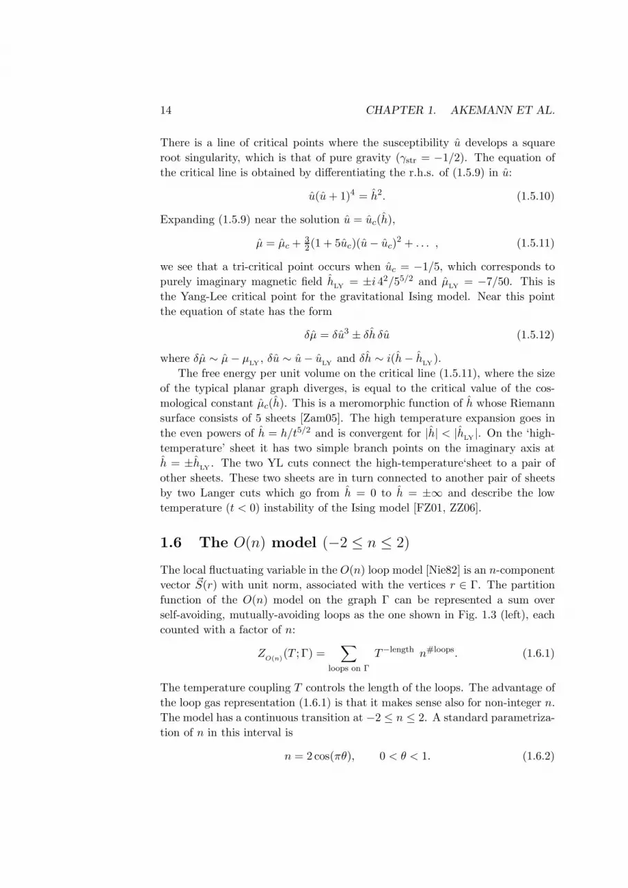
14 CHAPTER 1. AKEMANN ET AL.
There is a line of critical points where the susceptibility u develops a square
root singularity, which is that of pure gravity (γstr = −1/2). The equation of
the critical line is obtained by differentiating the r.h.s. of (1.5.9) in u:
u(u + 1)4 = h2. (1.5.10)
Expanding (1.5.9) near the solution u = uc(h),
µ = µc + 32(1 + 5uc)(u − uc)
2 + . . . , (1.5.11)
we see that a tri-critical point occurs when uc = −1/5, which corresponds to
purely imaginary magnetic field hLY = ±i 42/55/2 and µLY = −7/50. This is
the Yang-Lee critical point for the gravitational Ising model. Near this point
the equation of state has the form
δµ = δu3 ± δh δu (1.5.12)
where δµ ∼ µ − µLY
, δu ∼ u − uLY
and δh ∼ i(h − hLY
).
The free energy per unit volume on the critical line (1.5.11), where the size
of the typical planar graph diverges, is equal to the critical value of the cos-
mological constant µc(h). This is a meromorphic function of h whose Riemann
surface consists of 5 sheets [Zam05]. The high temperature expansion goes in
the even powers of h = h/t5/2 and is convergent for |h| < |hLY |. On the ‘high-
temperature’ sheet it has two simple branch points on the imaginary axis at
h = ±hLY
. The two YL cuts connect the high-temperature‘sheet to a pair of
other sheets. These two sheets are in turn connected to another pair of sheets
by two Langer cuts which go from h = 0 to h = ±∞ and describe the low
temperature (t < 0) instability of the Ising model [FZ01, ZZ06].
1.6 The O(n) model (−2 ≤ n ≤ 2)
The local fluctuating variable in the O(n) loop model [Nie82] is an n-component
vector ~S(r) with unit norm, associated with the vertices r ∈ Γ. The partition
function of the O(n) model on the graph Γ can be represented a sum over
self-avoiding, mutually-avoiding loops as the one shown in Fig. 1.3 (left), each
counted with a factor of n:
ZO(n)
(T ; Γ) =∑
loops on Γ
T−length n#loops. (1.6.1)
The temperature coupling T controls the length of the loops. The advantage of
the loop gas representation (1.6.1) is that it makes sense also for non-integer n.
The model has a continuous transition at −2 ≤ n ≤ 2. A standard parametriza-
tion of n in this interval is
n = 2cos(πθ), 0 < θ < 1. (1.6.2)

1.6. THE O(N) MODEL (−2 ≤ N ≤ 2) 15
The O(n) matrix model [Kos89a] generates planar graphs covered by loops
in the same way as the one-matrix model generates empty planar graphs. The
fluctuating variables are the hermitian matrix M and an O(n) vector ~Y, whose
components Y1, . . . ,Yn are hermitian matrices. All matrix variables are of size
N × N . The partition function is given by the integral
ZO(n)
N (T ) ∼∫
dM dnY e−β tr( 1
2M
2+ T2
~Y2− 13M
3−M~Y2). (1.6.3)
This integral can be considered as the partition function of a zero-dimensional
QFT with Feynman rules given in Fig. 1.3 (right).
aa
i ij
j
k
k
i ij
j
k
k
ij
ij
i i
j
T1/β
j
β β1/β
Figure 1.2: Left: A loop configuration on a disk with ordinary boundary condition.Right: Feynman rules for the O(n) matrix model.
The basic observable in the matrix model is the resolvent (1.4.11), evaluated
in the ensemble (1.6.3), which is the derivative of the disk partition function
with ordinary boundary condition for the O(n) spins. In terms of loop gas,
the ordinary boundary condition means that the loops in the bulk avoid the
boundary as they avoid the other loops and themselves.
The matrix integral measure becomes singular at M = T/2. We perform a
linear change of the variables M = T(
12 + X
)
which sends this singular point
to X = 0. After a suitable rescaling of ~Y and β, the matrix model partition
function takes the canonical form
ZO(n)
N (T ) ∼∫
dX dnYeβtr[−V (X)+X~Y2] , (1.6.4)
where V (x) is a cubic potential V (x) = −13T (x+ 1
2 )3 + 12(x+ 1
2 )2. Accordingly,
we redefine the spectral parameter by
z = T(
x + 12
)
. (1.6.5)
Now the one-point function with ordinary boundary condition is
W (x) =1
β〈trW〉 , W
def=
1
x − X. (1.6.6)
After integration with respect to the Y-matrices, the partition function takes
the form of a Coulomb gas
ZO(n)
N (T ) ∼∫ N
∏
j=1
dxi e−V (xi)
∏
i<j(xi − xj)2
∏
i,j(xi + xj)n/2. (1.6.7)
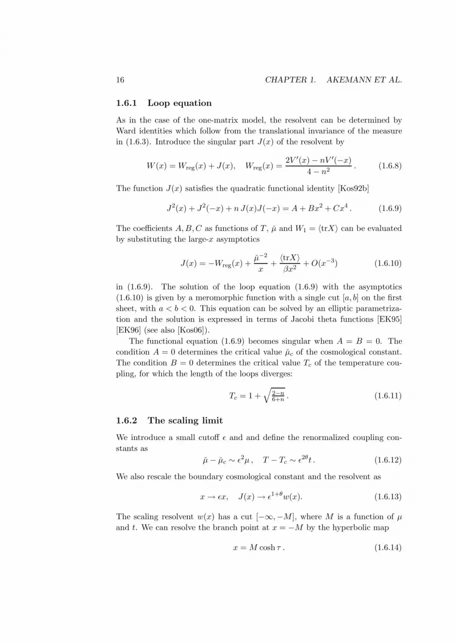
16 CHAPTER 1. AKEMANN ET AL.
1.6.1 Loop equation
As in the case of the one-matrix model, the resolvent can be determined by
Ward identities which follow from the translational invariance of the measure
in (1.6.3). Introduce the singular part J(x) of the resolvent by
W (x) = Wreg(x) + J(x), Wreg(x) =2V ′(x) − nV ′(−x)
4 − n2. (1.6.8)
The function J(x) satisfies the quadratic functional identity [Kos92b]
J2(x) + J2(−x) + n J(x)J(−x) = A + Bx2 + Cx4 . (1.6.9)
The coefficients A,B,C as functions of T , µ and W1 = 〈trX〉 can be evaluated
by substituting the large-x asymptotics
J(x) = −Wreg(x) +µ−2
x+
〈trX〉βx2
+ O(x−3) (1.6.10)
in (1.6.9). The solution of the loop equation (1.6.9) with the asymptotics
(1.6.10) is given by a meromorphic function with a single cut [a, b] on the first
sheet, with a < b < 0. This equation can be solved by an elliptic parametriza-
tion and the solution is expressed in terms of Jacobi theta functions [EK95]
[EK96] (see also [Kos06]).
The functional equation (1.6.9) becomes singular when A = B = 0. The
condition A = 0 determines the critical value µc of the cosmological constant.
The condition B = 0 determines the critical value Tc of the temperature cou-
pling, for which the length of the loops diverges:
Tc = 1 +√
2−n6+n . (1.6.11)
1.6.2 The scaling limit
We introduce a small cutoff ǫ and and define the renormalized coupling con-
stants as
µ − µc ∼ ǫ2µ , T − Tc ∼ ǫ2θt . (1.6.12)
We also rescale the boundary cosmological constant and the resolvent as
x → ǫx, J(x) → ǫ1+θw(x). (1.6.13)
The scaling resolvent w(x) has a cut [−∞,−M ], where M is a function of µ
and t. We can resolve the branch point at x = −M by the hyperbolic map
x = M cosh τ . (1.6.14)

1.6. THE O(N) MODEL (−2 ≤ N ≤ 2) 17
Then (1.6.9) becomes a quadratic functional equation for the entire function
w(τ) ≡ w[x(τ)]:
w2(τ + iπ) + w2(τ) + n w(τ + iπ)w(τ) = A1 + B1t M2 cosh2 τ . (1.6.15)
Here used the fact that near the critical temperature B ∼ T − Tc and the term
Cx4 vanishes. The unique solution, for some normalization of t, is
w(τ) = M1+θ cosh(1 + θ)τ + tM1−θ cosh(1 − θ)τ . (1.6.16)
The function M = M(µ, t) can be evaluated using the fact that the derivative
∂µw(x) depends on µ and t only through M . This is so if M satisfies the
transcendental equation
µ = (1 + θ)M2 − tM2−2θ. (1.6.17)
To summarize, the derivatives of the disk partition function in the scaling
limit, U(x, µ, t), are given in the following parametric form:
−∂xU |µ = M1+θcosh((1 + θτ) + t M1−θcosh(1 − θ)τ ,
−∂µU |x ∼ Mθ cosh θτ,
x = M cosh τ, (1.6.18)
with the function M(µ, t) determined from the transcendental equation (1.6.17).
The function M(t, µ) plays an important role in the solution. Its physical
meaning can be revealed by taking the limit x → ∞ of the bulk one-point
function −∂µU(x). Since x is coupled to the length of the boundary, in the
limit of large x the boundary shrinks and the result is the partition function
of the O(n) field on a sphere with two punctures, the susceptibility u(µ, t).
Expanding at x → ∞ we find
−∂µU ∼ xθ − M2θ x−θ + lower powers of x (1.6.19)
(the numerical coefficients are omitted). We conclude that the string suscepti-
bility is given, up to a normalization, by
u = M2θ. (1.6.20)
The normalization of u can be absorbed in the definition of the string coupling
constant gs ∼ 1/β. Thus the transcendental equation (1.6.17) for M gives the
equation of state of the loop gas on the sphere,
(1 + θ)u1θ − t u
1−θθ = µ . (1.6.21)

18 CHAPTER 1. AKEMANN ET AL.
The equation of state (1.6.21) has three singular points at which the three-
point function of the identity operator ∂µu diverges. The three points corre-
spond to the critical phases of the loop gas on the sphere.
1) At the critical point t = 0 the susceptibility scales as u ∼ µθ. This is
the dilute phase of the loop gas, in which the loops are critical, but occupy an
insignificant part of the lattice volume. By the KPZ relation (1.2.16), the O(n)
field is described by a CFT with central charge (1.2.8) with g = 1 + θ.
2) The dense phase is reached when t/xθ → −∞. In the dense phase the
loops remain critical but occupy almost all the lattice and the susceptibility
has different scaling, u ∼ µ1−θ
θ . The O(n) field in the dense phase is described
by a CFT with a lower central charge (1.2.8) with g = 1 − θ. Considered on
the interval −∞ < t < 0, the equation of state (1.6.21) describes the massless
thermal flow relating the dilute and the dense phases [Kos06].
3) At the third critical point ∂µM becomes singular but M itself remains
finite. Around this critical point µ − µc ∼ (M − Mc)2 + · · · , hence the scaling
of the susceptibility is that of pure gravity, u ∼ (µ − µc)1/2.
1.6.3 Other boundary conditions
Besides the ordinary boundary condition, there is a continuum of integrable
boundary conditions, which are generated by anisotropic boundary term [DJS09]
The loop gas expansion on the disk with such boundary condition can be for-
mulated in terms of loops of two different colors with fugacities n(1) and n(2) ,
such that n(1) + n(2) = n. The bulk is color blind, while the boundary interacts
differently with the loops of different color. A loop of color (α) acquires an
additional weight factor λ(α) each time it touches the boundary. The operator
in the matrix model creating a boundary segment with anisotropic boundary
condition is defined as follows. Decompose the vector ~Y into a sum of an
n(1)-component vector ~Y(1) and an n(2)-component vector ~Y(2) . Then the disk
one-point function with anisotropic boundary conditions is evaluated by
H(x, λ(1) , λ(2)) =1
β〈 trH 〉 , H
def=
1
x − X− λ(1)~Y2
(1) − λ(2)~Y2
(2)
. (1.6.22)
Nontrivial boundary critical behavior is achieved by tuning the two matter
boundary couplings λ(1) and λ(2) . The boundary phase diagram is qualitatively
the same as the one on the flat lattice [BHK09]. The boundary two-point func-
tions D0(x, y) = 1β
⟨
tr[
W(x)H(y)]
⟩
can be found as solutions of a functional
equations. The analysis of these equations away from the criticality allows to
draw the qualitative picture of bulk and boundary flows in the O(n) model
[BHK09].

1.7. THE SIX-VERTEX MODEL 19
1.7 The six-vertex model
The matrix model for the Baxter’s six-vertex model on planar graphs is a de-
formation of the O(2) model. Its partition function is given by [Kos00]
ZO(n)
N (T ) ∼∫
dX dYdY† eβtr[−V (X)+eiνX~YY
†+e−iνX~Y†
Y] . (1.7.1)
1.8 The q-state Potts model (0 < q < 4)
The local fluctuating variable in the q-state Potts model takes q discrete values
and the Hamiltonian has Sq symmetry. The partition function of the Potts
model is a sum over all clusters with fugacity q and weight 1/T for each link
occupied by the cluster. The corresponding matrix model is [Kaz88, Kos89c]
ZN (T ) ∼∫
dM dqY e−β tr( 1
2M
2+Pq
a=1(T2Y
2a− 1
3(M+Ya)3). (1.8.1)
The solution of the q-state Potts matrix model in the large N limit boils down
to a problem of matrix mean field. After a shift Ya → Ya − M the matrix
integral can be written as
Zq PottsN (T ) ∼
∫
dM e−β T+q
2TtrM2−βqW [M]), (1.8.2)
eβW [M] =
∫
dY eβtr(− 12T
Y2+ 1
3Y
3+ 1TMY). (1.8.3)
The effective action W defined by the last integral depends only on the eigenval-
ues of the matrix M. It was evaluated in the large N limit by the methods used
previously for the mean field problem in the large N gauge theory [BG80]. In
the scaling limit one obtains, after a redefinition of the spectral parameter, the
same functional equation as that for the O(n) model with n = q − 2 [Kos89c].
The analysis of the solution is however more delicate than in the case of the
O(n) matrix model. The complete solution of the q-state Potts matrix model
was found in [Dau94, ZJ01, EB99].
1.9 SOS and ADE matrix models
The rational theories of 2d QG are discretized by ensembles of planar graphs
embedded in ADE Dynkin diagrams [Kos90, Kos89b, Kos92b]. The correspond-
ing matrix models are constructed in [Kos92a].
More generally, for a discrete target space representing a graph G one as-
sociates a hermitian matrix Xa with each node a ∈ G and a complex matrix

20 REFERENCES
a aa
b
aa
a b a
aij
ij
T1/β
j
β1/β
i i
j
i ij
j
k
k
β
i ij
j
k
k
Figure 1.3: Feynman rules for the matrix model with target space G.
Y<ab> = Y†<ba> with each link <ab>. The matrix model that generates planar
graphs embedded in the graph G is defined by the partition function
ZG
N (β, T ) =
∫
∏
a∈GdXa e−βtrV (Xa)
∏
<ab>
etr(XaY<ab>Y<ba>+Y<ab>XbY<ba>). (1.9.1)
For trivalent graphs the potential V is the same as that of the O(n) model.
The matrix model has an interesting continuum limit if the graph G is an ADE
or ADE Dynkin diagram. The SOS model, which is a discretization of the
gaussian field with a charge at infinity [Nie82], corresponds to an infinite target
space Z [Kos92b]. Matrix models with semi-infinite target spaces A∞ and D∞were studied in [KP07].
References
[ADF85] Jan Ambjorn, B. Durhuus, and J. Frohlich. Diseases of Triangulated RandomSurface Models, and Possible Cures. Nucl. Phys., B257:433, 1985.
[BG80] E. Brezin and David J. Gross. The External Field Problem in the Large N Limitof QCD. Phys. Lett., B97:120, 1980.
[BHK09] Jean-Emile Bourgine, Kazuo Hosomichi, and Ivan Kostov. Boundary transitionsof the O(n) model on a dynamical lattice. 2009, hep-th/0910.1581.
[BIPZ78] E. Brezin, C. Itzykson, G. Parisi, and J. B. Zuber. Planar Diagrams. Commun.Math. Phys., 59:35, 1978.
[BK87] D. Boulatov and V. Kazakov. The Ising Model on Random Planar Lattice: TheStructure of Phase Transition and the Exact Critical Exponents. Phys. Lett.,186B:379, 1987.
[BKKM86] D. Boulatov, V. Kazakov, I. Kostov, and A. Migdal. Analytical and NumericalStudy of the Model of Dynamically Triangulated Random Surfaces. Nucl. Phys.,B275:641, 1986.
[CGM90] Cedomir Crnkovic, Paul H. Ginsparg, and Gregory W. Moore. The Ising Model,the Yang-Lee Edge Singularity, and 2D Quantum Gravity. Phys. Lett., B237:196,1990.
[Dau94] Jean-Marc Daul. Q states Potts model on a random planar lattice. 1994, hep-th/9502014.
[Dav85a] F. David. A Model of Random Surfaces with Nontrivial Critical Behavior. Nucl.Phys., B257:543, 1985.
[Dav85b] F. David. Planar Diagrams, Two-Dimensional Lattice Gravity and Surface Mod-els. Nucl. Phys., B257:45, 1985.

REFERENCES 21
[Dav88] F. David. Conformal Field Theories Coupled to 2D Gravity in the ConformalGauge. Mod. Phys. Lett., A3:1651, 1988.
[DFGZJ95] P. Di Francesco, P. Ginsparg, and J. Zinn-Justin. 2d gravity and random matrices.Physics Reports, 254:1–133, 1995.
[DJS09] Jerome Dubail, Jesper Lykke Jacobsen, and Hubert Saleur. Exact solution ofthe anisotropic special transition in the o(n) model in two dimensions. PhysicalReview Letters, 103(14):145701, 2009.
[DK88] Bertrand Duplantier and I. Kostov. Conformal spectra of polymers on a randomsurface. Phys. Rev. Lett., 61:1433, 1988.
[DK89] J. Distler and H. Kawai. Conformal field theory and 2d quantum gravity. NuclearPhysics B, 321:509–527, 1989.
[DK90] Bertrand Duplantier and Ivan K. Kostov. Geometrical critical phenomena on arandom surface of arbitrary genus. Nucl. Phys., B340:491–541, 1990.
[DKK93] J.M. Daul, V. Kazakov, and I. Kostov. Rational theories of 2d gravity from thetwo-matrix model. Nucl.Phys., B409:311–338, 1993, hep-th/9303093.
[EB99] B. Eynard and G. Bonnet. The Potts-q random matrix model : loop equa-tions, critical exponents, and rational case. Phys. Lett., B463:273–279, 1999,hep-th/9906130.
[EK95] B. Eynard and C. Kristjansen. Exact Solution of the O(n) Model on a RandomLattice. Nucl. Phys., B455:577–618, 1995, hep-th/9506193.
[EK96] B. Eynard and C. Kristjansen. More on the exact solution of the O(n) model ona random lattice and an investigation of the case |n| > 2. Nucl. Phys., B466:463–487, 1996, hep-th/9512052.
[FZ01] P. Fonseca and A. Zamolodchikov. Ising field theory in a magnetic field: Analyticproperties of the free energy. 2001, hep-th/0112167.
[GM93] Paul H. Ginsparg and Gregory W. Moore. Lectures on 2-D gravity and 2-D stringtheory. 1993, hep-th/9304011.
[Kaz85] V. Kazakov. Bilocal Regularization of Models of Random Surfaces. Phys. Lett.,B150:282–284, 1985.
[Kaz86] V. Kazakov. Ising model on a dynamical planar random lattice: Exact solution.Phys. Lett., A119:140–144, 1986.
[Kaz88] V. Kazakov. Exactly solvable Potts models, bond and tree percolation on dy-namical (random) planar surface. Nucl. Phys. B (Proc. Suppl.), 4:93–97, 1988.
[Kaz89] V. Kazakov. The Appearance of Matter Fields from Quantum Fluctuations of2D Gravity. Mod. Phys. Lett., A4:2125, 1989.
[KKM85] V. Kazakov, I. Kostov, and A. Migdal. Critical Properties of Randomly Triangu-lated Planar Random Surfaces. Phys. Lett., B157:295–300, 1985.
[Kle95] Igor R. Klebanov. Touching random surfaces and Liouville gravity. Phys. Rev.,D51:1836–1841, 1995, hep-th/9407167.
[KM87] I. Kostov and M. L. Mehta. Random surfaces of arbitrary genus: exact resultsfor D=0 and -2 dimansions. Phys. Lett., B189:118–124, 1987.
[Kos89a] I. Kostov. O(n) vector model on a planar random surface: spectrum of anomalousdimensions. Mod. Phys. Lett., A4:217, 1989.
[Kos89b] I. Kostov. The ADE face models on a fluctuating planar lattice. Nucl. Phys.,B326:583, 1989.

22 REFERENCES
[Kos89c] I. K. Kostov. Random surfaces, solvable lattice models and discrete quantumgravity in two dimensions. Nuclear Physics B (Proc. Suppl.), 10A:295–322, 1989.Lecture given at GIFT Int. Seminar on Nonperturbative Aspects of the StandardModel, Jaca, Spain, Jun 6-11, 1988.
[Kos90] I. Kostov. Strings embedded in Dynkin diagrams. 1990. Lecture given at CargeseMtg. on Random Surfaces, Quantum Gravity and Strings, Cargese, France, May27 - Jun 2, 1990.
[Kos92a] I. Kostov. Gauge invariant matrix model for the A-D-E closed strings. Phys.Lett., B297:74–81, 1992, hep-th/9208053.
[Kos92b] I. Kostov. Strings with discrete target space. Nucl. Phys., B376:539–598, 1992,hep-th/9112059.
[Kos00] I. Kostov. Exact solution of the six-vertex model on a random lattice. Nucl.Phys., B575:513–534, 2000, hep-th/9911023.
[Kos06] I. Kostov. Thermal flow in the gravitational O(n) model. 2006, hep-th/0602075.
[KP07] I. Kostov and V.B. Petkova. Non-rational 2d quantum gravity ii. target spacecft. Nucl.Phys.B, 769:175–216, 2007, hep-th/0609020.
[KPZ88] V. G. Knizhnik, Alexander M. Polyakov, and A. B. Zamolodchikov. Fractalstructure of 2d-quantum gravity. Mod. Phys. Lett., A3:819, 1988.
[KS92] I. Kostov and Matthias Staudacher. Multicritical phases of the O(n) model on arandom lattice. Nucl. Phys., B384:459–483, 1992, hep-th/9203030.
[Nie82] Bernard Nienhuis. Exact critical point and critical exponents of o(n) models intwo dimensions. Phys. Rev. Lett., 49(15):1062–1065, Oct 1982.
[Pol81] Alexander M. Polyakov. Quantum geometry of bosonic strings. Phys. Lett.,B103:207–210, 1981.
[Sta90] Matthias Staudacher. The Yang-Lee edge singularity on a dynamical planarrandom surface. Nucl. Phys., B336:349, 1990.
[tH74] G. t Hooft. A planar diagram theory for strong interactions. Nuclear Physics B,72:461–473, 1974.
[Zam05] Al. Zamolodchikov. Thermodynamics of the gravitational ising model. A talkgiven at ENS, Paris (unpublished), 2005.
[Zam07] Al. Zamolodchikov. Gravitational Yang-Lee model: Four point function. Theor.Math. Phys., 151:439–458, 2007, hep-th/0604158.
[ZJ01] P. Zinn-Justin. The dilute potts model on random surfaces. Journal of StatisticalPhysics, 98:245, 2001.
[ZZ06] A. Zamolodchikov and Al. Zamolodchikov. Decay of metastable vacuum in Liou-ville gravity. 2006, hep-th/0608196.


