Embed Size (px)
Citation preview
B′′H
Two-Photon Frequency Comb Spectroscopyof Atomic Hydrogen
Alexey Grinin
Munich 2020

Two-Photon Frequency Comb Spectroscopyof Atomic Hydrogen
Alexey Grinin
Dissertationperformed in the Laser Spectroscopy Division
of the Max-Planck-Institute for Quantum OpticsGarching
presented to the Faculty of Physicsof the Ludwig-Maximilians-Universität
München
byAlexey Grininfrom Gorbunki
Munich, June 30th, 2020

Erstgutachter: Prof. Dr. Theodor W. HänschZweitgutachter: Prof. Dr. Randolf PohlTag der mündlichen Prüfung: 18. August 2020
ZusammenfassungQuantenelektrodynamik (QED) wird oft als die Krone der modernen Physik bezeich-net, da sie mit erstaunlicher Genauigkeit experimentelle Ergebnisse vorhersagt. Fürgegebene Werte der entsprechenden Naturkonstanten können zum Beispiel Energie-niveaus im Wasserstoffatom mit Hilfe der QED auf bis zu 13 Stellen genau berechnetwerden. Die Entwicklung der QED ging Seite an Seite mit der Präzisionsspektrosko-pie des einfachsten Atoms im Universum, des Wasserstoffatoms (H). Auch heutebleibt die Wasserstoffspektroskopie unersetzlich für die experimentelle Verifizierung(Falsifizierung) der Quantenelektrodynamik. Um die Energieniveaus im Wasserstoffzu berechnen, benötigt die Theorie je nach Genauigkeit einen oder mehrere Pa-rameter, fundamentale Naturkonstanten, die experimentell bestimmt werden müs-sen. Die Wasserstoffspektroskopie liefert zwei von ihnen mit höchster Präzision, dieRydbergkonstante R∞ und den Proton-Ladungsradius rp (muonischer Wasserstoff).Zwei weitere Konstanten sind zur Zeit für die Bestimmung der Energieneveaus nötig.Das Elektron zu Proton Massenverhältnis me/mp und die Feinstrukturkonstante αwerden mit Hilfe von Penningtrap- und Atominterferometrieexperimenten bestimmt[1, 2]. Mit fortschreitender Genauigkeit werden kleinere Effekte berücksichtigt wer-den müssen und entsprechend weitere Naturkonstanten benötigt (z.B. das Verhältnisder Elektronmasse zur Planck Konstanten me/h).Die Vermessung der Lambverschiebung im muonischen Wasserstoffatom in 2010 [3],führte zu einem unerwartetenWiderspruch, der auf den Namen Proton Radius Puzzle(PRP) getauft wurde. Im kurzlebigen muonischen Wasserstoff ist das Elektron durchdas 200-fach schwerere kurzlebige Muon substituiert. Dadurch ist das Muon etwa 200mal näher zum Proton und die Abweichung von der punktförmigen Ladungsvertei-lung des Protons (finite proton size correction) sieben Grössenordnungen grösser alsim normalen Wasserstoffatom. Dadurch können diese winzige Energieverschiebungund der Proton-Ladungsradius viel genauer gemessen werden, als das bis dahin mitallen Wasserstoffübergängen möglich war. Allerdings wich der so ermittelte Proton-Ladungsradius sieben Standardabweichungen von dem Wert ab, den das Committeeon Data for Science and Technology (CODATA) mit Hilfe der Wasserstoffspektro-skopiedaten und der Streuungsexperimente an Protonen ermittelt hat [4]. Drei neueMessungen sind inzwischen dazugekommen. Während die Vermessung des 2S–4PÜbergangs im Wasserstoffatom [5] und der 2S–2P Übergang [6] mit dem muonischenWert übereinstimmte, unterstützte das 1S–3S Experiment am LKB in Paris [7] denCODATA 2014 Wert. Die letzte CODATA 2018 [8] Auswertung ist inzwischen onli-ne veröffentlicht worden. Der neue Wert des RMS Proton-Ladungsradius stimmt mitden Messungungen des 2S–4P [5] und des 2S–2P Übergänge [6] überein. Allerdingssind keine Details zur Auswertung zur Zeit vorhanden.Als Ergebnis dieser Arbeit wurde die Unsicherheit des Proton-Ladungsradius undder Rydbergkonstante um einen Faktor von zwei reduziert, verglichen mit der kom-binierten Unsicherheit aller im Wasserstoffatom vermessenen Übergänge, inklusiveder kürzlich publizierten Erbebnisse am 2S–4P, 2S–2P und 1S–3S Übergängen. Da-mit ist es die zweitgenaueste Messung im Wasserstoff, die nur der Vermessung desmetastabilen 1S–2S Übergangs [9], an Präzision unterliegt. Es ist der erste Über-gang im Wasserstoff, der von zwei unabhängigen Gruppen und mit unterschiedlichenMethoden aber mit einer für das Proton Radius Rätsel signifikanten Unsicherheit,gemessen wurde. Die Diskrepanz der Ergebnisse von 2.1σ kombinierten Standardab-weichungen deutet darauf hin, dass es sich bei dem Rätsel um ein experimentellesProblem handeln könnte und ermöglicht durch Vergleich und eine wiederholte Ana-lyse der systematischen Fehler, das Problem ausfindig zu machen. Es wurde viel
experimentelle Arbeit darauf aufgewendet, alle relevanten systematischen Frequenz-verschiebungen möglichst klein (kleiner als die PRP Diskrepanz von 7 kHz für 1S–3SÜbergang) zu halten. Dies wurde vor allem durch einen kryogenen Atomstahl und einverbessertes Lasersystem möglich. Alle signifikanten systematischen Effekte (inclu-sive der Druckverschiebung) wurden experimentell und simulationsunabhängig (inerster Ordnung) bestimmt. Die Auflösung der natürlichen Linienbreite von 1 MHzauf einen moderaten Wert von 10−3 deutet auf weiteres Potenzial dieses Experi-ments hin. Ferner demonstriert diese Arbeit zum ersten Mal die hochauflösende Fre-quenzkammspektroskopie im Ultraviolettbereich mit Subkilohertz-Unsicherheit undist damit wegweisend für die Präzisionsspektroskopie im UV und DUV Bereich, wonur die Erzeugung von höheren Harmonischen als Laserquelle zur Zeit zur Verfügungstehen.Unser Ergebnis unterstützt (1.9σ) den Proton-Ladungsradius aus der Spektrosko-pie am muonischen Wasserstoff und weicht von dem CODATA 2014 Wert um 2.9σkombinierte Standardabweichungen ab. Der Vergleich mit der neuen Messung des1S–3S Übergangs [7] is limitiert durch die 3.5-fach größere Unsicherheit in [7] undergibt eine Abweichung von 2.1σ kombinierten Standardabweichungen. Wir bekom-men die folgende absolute Frequenz für den 1S–3S (F = 1 zu F = 1) Übergang imWasserstoff:
f1S–3S(F =1) = 2 922 742 936 716.72(72) kHz. (0.1)
Nach Abzug der Hyperfeinverschiebung von −341 949 069.6(8) Hz [10] ermitteln wirdie Zentroidfrequenz des 1S–3S Übergangs zu:
f1S–3S(centroid) = 2 922 743 278 665.79(72) kHz. (0.2)
Mit Hilfe der 1S–2S Übergangsfrequenz und der Wasserstoffatomtheorie (zusam-mengefasst in [4]) bekommen wir verbesserte Werte der Rydbergkonstanten und desProton-Ladungsradius:
R∞ = 10973731.568226(38) m−1 (0.3)
rp = 0.8482(38) fm. (0.4)
AbstractQuantum electrodynamics (QED) is often considered to be the crown of modernphysics in that it is able to predict experiments with astonishing accuracy, reach-ing, for instance, up to 13 digits of precision for hydrogen energy levels (assumingexact values of required fundamental constants). Due to the simplicity of the hydro-gen atom, the development of QED went-side-by side with precision spectroscopy inhydrogen and remains one of the corner stones for testing QED. However the theorydepends on four parameters, fundamental constants, which have to be determinedexperimentally. Precision hydrogen spectroscopy is best at measuring the Rydbergconstant R∞, the most precisely known fundamental constant, and the RMS protoncharge radius rp. The electron to proton mass ratio me/mp and the fine structureconstant α are determined in precision Penning trap and atom interferometry exper-iments [1, 2]. At the current level of accuracy the knowledge of these four constantssuffices. With higher precision, additional constants, such as the electron mass toPlanck constant ratio (me/h), are required.A new intriguing problem, which arose from spectroscopy of muonic hydrogen in2010, attracted broad interest and is referred to as the Proton Radius Puzzle (PRP).In muonic hydrogen the electron of the hydrogen atom is replaced by the 200 timesheavier, short lived muon. As a result of the increased mass the muons orbit is alsoapprox. 200 times closer to the proton. This amplifies the finite proton size correctionby almost seven orders of magnitude and allows for very precise determination of rp.The measurement of the 2S–2P transition in muonic hydrogen [3] determined theproton charge radius to be seven combined standard deviations smaller than the valuedetermined in the global adjustment of fundamental constants [4] by the Committeeon Data for Science and Technology (CODATA). Three recent measurements inhydrogen with significantly small uncertainties make the problem even more puzzling.While the 2S–4P measurement[5] and the 2S–2P Lamb shift measurement [6] areconsistent with the muonic hydrogen value, the 1S–3S [7] measurement supports theCODATA 2014 value. The most recent CODATA 2018 evaluation is meanwhile alsoavailable online and agrees with the recent measurements of the 2S–4P [5] and the2S–2P Lamb shift measurements [6]. However, details of the analysis are not yetavailable.One of the important results of this work is a significant improvement of the accu-racy of the Rydberg constant and the proton charge radius. The uncertainties onthe RMS proton charge radius and the Rydberg constant derived from it are 2 timesmore precise than the overall previous hydrogen world data including the recent mea-surements of the 1S–3S, 2S–2P and 2S–4P transitions. It is the second most precisemeasurement in hydrogen after the 1S–2S [9], which has orders of magnitude smallerline width than all other transitions. It is the first measurement in hydrogen, whichhas been performed by two independent groups with different methods and sufficientuncertainty to check consistency within the hydrogen data which is used for protoncharge radius determination and therefore sheds light onto possible experimental na-ture of the discrepancy. All systematic frequency shifts have been reduced to valuessmaller than the corresponding PRP discrepancy of 7 kHz. All significant system-atic frequency shifts (including pressure shift) have been measured experimentallyand do not rely on simulation to first order. We split the 1 MHz broad 1S–3S lineby a moderate value of only about 10−3. Finally, this work demonstrates the firsthigh-resolution spectroscopy below 1 kHz level with a harmonic frequency comb inUV in hydrogen, which is important for future precision spectroscopy experimentsin UV and DUV region, where only high harmonic generation as a laser source is
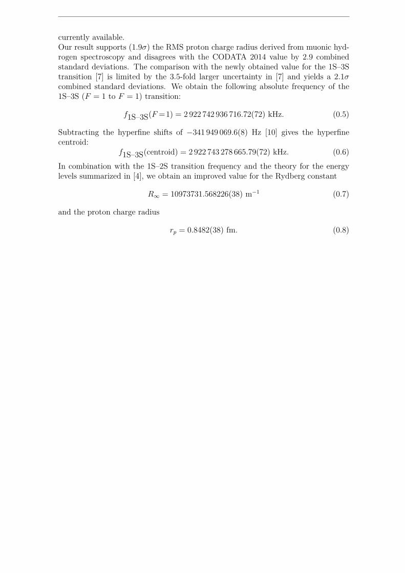
currently available.Our result supports (1.9σ) the RMS proton charge radius derived from muonic hyd-rogen spectroscopy and disagrees with the CODATA 2014 value by 2.9 combinedstandard deviations. The comparison with the newly obtained value for the 1S–3Stransition [7] is limited by the 3.5-fold larger uncertainty in [7] and yields a 2.1σcombined standard deviations. We obtain the following absolute frequency of the1S–3S (F = 1 to F = 1) transition:
f1S–3S(F =1) = 2 922 742 936 716.72(72) kHz. (0.5)
Subtracting the hyperfine shifts of −341 949 069.6(8) Hz [10] gives the hyperfinecentroid:
f1S–3S(centroid) = 2 922 743 278 665.79(72) kHz. (0.6)
In combination with the 1S–2S transition frequency and the theory for the energylevels summarized in [4], we obtain an improved value for the Rydberg constant
R∞ = 10973731.568226(38) m−1 (0.7)
and the proton charge radius
rp = 0.8482(38) fm. (0.8)
Contents
List of Figures iii
1. Precision Hydrogen Spectroscopy 11.1. The Historic Interplay between Hydrogen Spectroscopy and QED . . 11.2. QED Description of the Energy Levels in Hydrogen . . . . . . . . . . 51.3. Proton Radius Puzzle . . . . . . . . . . . . . . . . . . . . . . . . . . . 61.4. Advances of the Garching 1S–3S Setup . . . . . . . . . . . . . . . . . 9
2. Two-photon Direct Frequency Comb Spectroscopy 112.1. Frequency Combs in Spectroscopy . . . . . . . . . . . . . . . . . . . . 112.2. Basics of Frequency Combs . . . . . . . . . . . . . . . . . . . . . . . . 122.3. Continuous Wave Two-Photon Spectroscopy . . . . . . . . . . . . . . 142.4. Two-Photon Frequency Comb Spectroscopy . . . . . . . . . . . . . . 222.5. Monte Carlo simulations . . . . . . . . . . . . . . . . . . . . . . . . . 27
3. Experimental setup 313.1. Frequency measurement . . . . . . . . . . . . . . . . . . . . . . . . . 313.2. Laser system . . . . . . . . . . . . . . . . . . . . . . . . . . . . . . . 343.3. Mode suppression . . . . . . . . . . . . . . . . . . . . . . . . . . . . 403.4. Vacuum system and enhancement cavity . . . . . . . . . . . . . . . . 423.5. Atomic hydrogen beam . . . . . . . . . . . . . . . . . . . . . . . . . 463.6. Fluorescence detection . . . . . . . . . . . . . . . . . . . . . . . . . . 49
4. Data Evaluation 554.1. Data Description . . . . . . . . . . . . . . . . . . . . . . . . . . . . . 554.2. Line fitting and normalization . . . . . . . . . . . . . . . . . . . . . . 564.3. Line width . . . . . . . . . . . . . . . . . . . . . . . . . . . . . . . . 594.4. Global fitting procedure . . . . . . . . . . . . . . . . . . . . . . . . . 61
5. Systematic Uncertainties Analysis 655.1. Chirp induced residual first-order Doppler shift . . . . . . . . . . . . 655.2. AC-Stark shift . . . . . . . . . . . . . . . . . . . . . . . . . . . . . . 745.3. Second-order Doppler shift . . . . . . . . . . . . . . . . . . . . . . . 775.4. Pressure shift . . . . . . . . . . . . . . . . . . . . . . . . . . . . . . . 815.5. DC-Stark shift . . . . . . . . . . . . . . . . . . . . . . . . . . . . . . 845.6. Zeeman shift . . . . . . . . . . . . . . . . . . . . . . . . . . . . . . . 885.7. Line distorting effects . . . . . . . . . . . . . . . . . . . . . . . . . . 90
i
Contents
5.8. Quantum interference . . . . . . . . . . . . . . . . . . . . . . . . . . 925.9. Incoherent line pulling . . . . . . . . . . . . . . . . . . . . . . . . . . 94
5.9.1. Other line components . . . . . . . . . . . . . . . . . . . . . . 945.9.2. Forbidden ∆F = 1 components . . . . . . . . . . . . . . . . . 965.9.3. Cavity modulation side bands . . . . . . . . . . . . . . . . . . 99
5.10. Tilted wave fronts . . . . . . . . . . . . . . . . . . . . . . . . . . . . 1015.11. Cross-talks between different systematic effects . . . . . . . . . . . . 1045.12. Results and Error Budget . . . . . . . . . . . . . . . . . . . . . . . . 109
6. Conclusions and Outlook 1116.1. Discussion of Measurement Results . . . . . . . . . . . . . . . . . . . 1116.2. Frequency Comb Spectroscopy Technique Investigation Results . . . . 1136.3. Suggestions for Future Improvements . . . . . . . . . . . . . . . . . . 115
Appendix 117
A. Enhancement Cavity Characterization 117A.1. Transmission Measurement . . . . . . . . . . . . . . . . . . . . . . . . 117A.2. Cavity Waist Measurement and Mode Matching . . . . . . . . . . . . 118
B. AC Stark Shift Derivation 121B.1. Fourth Order AC Stark Shift . . . . . . . . . . . . . . . . . . . . . . . 122
Bibliography 129
Acknowledgments 139
List of publications and presentations 141
Declaration of Originality 145
ii
List of Figures
1.1. Hydrogen energy diagram showing levels with principal quantum num-ber n ≤ 3. . . . . . . . . . . . . . . . . . . . . . . . . . . . . . . . . . 3
1.2. Proton charge radius . . . . . . . . . . . . . . . . . . . . . . . . . . . 7
2.1. Frequency comb spectrum . . . . . . . . . . . . . . . . . . . . . . . . 122.2. Two-photon excitation . . . . . . . . . . . . . . . . . . . . . . . . . . 152.3. Two-photon excitation types . . . . . . . . . . . . . . . . . . . . . . . 172.4. Doppler free to Doppler broadened contrast comparison. . . . . . . . 222.5. Principle of the two-photon frequency comb spectroscopy. . . . . . . . 242.6. Steady state solution for DFCS . . . . . . . . . . . . . . . . . . . . . 24
3.1. Experimental set–up . . . . . . . . . . . . . . . . . . . . . . . . . . . 323.2. Full frequency scan with all fine- and hyperfine 1s–3S and 1S–3D
transitions . . . . . . . . . . . . . . . . . . . . . . . . . . . . . . . . . 343.3. Comb spectra . . . . . . . . . . . . . . . . . . . . . . . . . . . . . . . 363.4. Self-phase modulation simulation . . . . . . . . . . . . . . . . . . . . 383.5. Vacuum system . . . . . . . . . . . . . . . . . . . . . . . . . . . . . . 423.6. Differential pumping system . . . . . . . . . . . . . . . . . . . . . . . 443.7. Hydrogen dissociation system . . . . . . . . . . . . . . . . . . . . . . 473.8. Temperature dependence of the count rates . . . . . . . . . . . . . . . 483.9. Drawing of the PCV and detection scheme . . . . . . . . . . . . . . . 503.10. Detection profile . . . . . . . . . . . . . . . . . . . . . . . . . . . . . 51
4.1. Histogram of valid data points . . . . . . . . . . . . . . . . . . . . . . 564.2. Normalization example scan . . . . . . . . . . . . . . . . . . . . . . . 574.3. χ2 distribution analysis . . . . . . . . . . . . . . . . . . . . . . . . . . 584.4. Correlation between DB and DF count rates . . . . . . . . . . . . . . 594.5. Average Line and residuals . . . . . . . . . . . . . . . . . . . . . . . . 604.6. Line widths analysis . . . . . . . . . . . . . . . . . . . . . . . . . . . 614.7. Global fit χ2-distribution analysis . . . . . . . . . . . . . . . . . . . . 63
5.1. CIFODS principle . . . . . . . . . . . . . . . . . . . . . . . . . . . . . 665.2. CIFODS Monte Carlo simulation . . . . . . . . . . . . . . . . . . . . 685.3. Measurement of the CIFODS as a function of position . . . . . . . . . 695.4. Linearity of the CIFODS effect . . . . . . . . . . . . . . . . . . . . . 705.5. CIFODS interpolation . . . . . . . . . . . . . . . . . . . . . . . . . . 715.6. Experimental chirp distribution . . . . . . . . . . . . . . . . . . . . . 72
iii
List of Figures
5.7. AC-Stark shift extrapolation . . . . . . . . . . . . . . . . . . . . . . . 755.8. SOD crossover velocity . . . . . . . . . . . . . . . . . . . . . . . . . . 785.9. SOD simulation . . . . . . . . . . . . . . . . . . . . . . . . . . . . . . 795.10. SOD extrapolation . . . . . . . . . . . . . . . . . . . . . . . . . . . . 805.11. Amplitudes ratio vs. temperature . . . . . . . . . . . . . . . . . . . . 825.12. Pressure shift extrapolation . . . . . . . . . . . . . . . . . . . . . . . 835.13. Charging up of the nozzle . . . . . . . . . . . . . . . . . . . . . . . . 855.14. DC-Stark shift screening and compensation . . . . . . . . . . . . . . . 865.15. DC-Stark shift measurement . . . . . . . . . . . . . . . . . . . . . . . 875.16. SOD line shape distortion . . . . . . . . . . . . . . . . . . . . . . . . 915.17. SOD line shape distortion frequency shift . . . . . . . . . . . . . . . . 925.18. Quantum interference . . . . . . . . . . . . . . . . . . . . . . . . . . . 935.19. Tilted wave fronts Doppler shift . . . . . . . . . . . . . . . . . . . . . 1015.20. Tilted wave fronts Doppler shift extrapolation . . . . . . . . . . . . . 1045.21. SOD mimics CIFODS . . . . . . . . . . . . . . . . . . . . . . . . . . 106
A.1. A scheme of the UV enhancement cavity of the 1S–3S experimenttogether with a beam profiler/power meter . . . . . . . . . . . . . . . 118
A.2. Determination of the cavity waist using a beam profiler . . . . . . . . 119A.3. Enhancement cavity transmitted power cavity modes . . . . . . . . . 120A.4. White light interferogram of the cavity mirrors . . . . . . . . . . . . . 121
iv
1. Precision Hydrogen Spectroscopy
1.1. The Historic Interplay between HydrogenSpectroscopy and QED
The hydrogen atom has played without doubt a key role in the development of atomicphysics and quantum mechanics [11]. Being a two-body system it was possible tocalculate its spectrum analytically and thus over a time span of 60 years a series ofrefinements of theory and experiment has been performed, finally resulting in theformulation of the quantum electrodynamics (QED), which is often stated as the besttheory in physics. It is capable of predicting the energy levels of atomic hydrogenand the electron g factor with an incredible accuracy and served as the blueprint forother quantum field theories.
The first detailed spectrum of hydrogen has been published by Anders JonasÅngström in 1862 [12]. Johann Jakob Balmer in 1885 provided an empirical formulafor the wavelengths of the Balmer series (n = 3, 4, 5, . . .→ n = 2, [13]), observed inthe spectrum of hydrogen and Johannes Robert Rydberg generalized it to include allwavelengths in 1888. In it’s modern version the Rydberg formula for the hydrogenenergy levels is:
En = −R∞n2 (1.1)
Where En is the energy of the level with the principal quantum number n and R∞the Rydberg constant.
The advances in the understanding of the structure of atoms through scatteringexperiments by Ernest Rutherford in 1911 built the ground for the developmentof the first quantum theory by Niels Bohr in 1913. Bohr’s atomic model assumesa heavy nucleus consisting of a positively charged proton and a light negativelycharged electron orbiting around the proton bound by the Coulomb force. Theangular momentum of the electron is assumed to take only integer numbers of thePlanck constant ~ and can be interpreted as a standing matter wave with the deBroglie wavelength.
The interpretation of the electron as a standing matter wave lead to a search fora matter wave equation, which was formulated by Erwin Schrödinger in 1926.
i~∂
∂tΨ (~r, t) =
[−~2
2m ∇2 + V (~r, t)
]Ψ (~r, t) (1.2)
Here Ψ (~r, t) is the complex wave function of the electron (or any other quantumparticle), the square modulus of which is interpreted (Max Born) as the probabi-
1
1. Precision Hydrogen Spectroscopy
lity distribution of the electron to be at a certain place ~r at the time t. Just astrajectories were now replaced by probability distributions, physical quantities likethe kinetic energy and potential were replaced by operators −~2
2m∇2, V (~r, r) (for in-
stance Coulomb potential). Schrödinger’s equation 1.2 remains the working horseof quantum mechanical calculations till today and is by no means restricted to thesimple hydrogen atom. The Rydberg formula 1.1 could be derived formally withit and also the line intensities were explained for the first time. The solutions ofthe Schrödinger equation have besides the principal quantum number n two angu-lar momentum quantum numbers l = 0, 1, . . . , n and ml = −l,−l + 1, . . . , l − 1, l.The energies of the levels with the same principal quantum number n however arepredicted by the Schrödinger equation to have the same energy, i.e. to be degenerate.
Already in 1887, long before Bohr and Schrödinger proposed their theories, Michel-son and Morley [14] showed by means of Fourier spectroscopy that the Balmer-α line(n = 3 → n = 2) is a doublet. This so called fine splitting is a relativistic correc-tion due to electrons motion and its spin, which lifts the degeneracy of the levelswith the same principal quantum number n but different total angular momentum(J = L+S) quantum number j (capital letters denote operators, corresponding smallletters their eigenvalues). The electron’s spin, an intrinsic angular momentum of theelectron, which has no classical equivalent was first observed in the famous Stern-Gerlach experiment in 1921, predating the Schrödinger theory and was postulated byUhlenbeck and Goudsmit in 1925. It was added ad hoc to the Schrödinger equation.Using the relativistic energy momentum relation other relativistic corrections couldalso be derived for special cases (Arnold Sommerfeld). While the spin-orbit correc-tion separately depends on all quantum numbers (n,l,s) and the relativistic velocitychange of the electron mass depends on n and l, only the total angular momentumquantum number j remains in their sum. The fine splitting scales with the squareof the fine-structure constant α ≈ 1/137 and with the fourth power of the chargenumber Z (for hydrogen-like ions with larger nuclear charge).
∆En,l,j = α2(
34n −
1j − 1/2
)Z4
n3 2πhcR∞ (1.3)
Here ∆En,l,j is the energy difference between fine structure components (j = l+ 1/2and j = l − 1/2), Z is the nucleus charge.
A similar though several orders of magnitude smaller effect to the spin–orbitcoupling is the hyperfine structure, which is due to the coupling between the nuclearspin I and the angular momentum L and spin S of the electron (total angularmomentum F = L+S+I). First measurements were already performed by Michelsonin 1881 but could be only explained when Wolfgang Pauli proposed the nuclear spinin 1924.
These important results could first rigorously be derived by Paul Dirac in 1928.The Dirac equation was the first fully relativistic matter wave equation, satisfyinginherently the Lorentz invariance and relativistic energy momentum relation. The
2
1.1. The Historic Interplay between Hydrogen Spectroscopy and QED
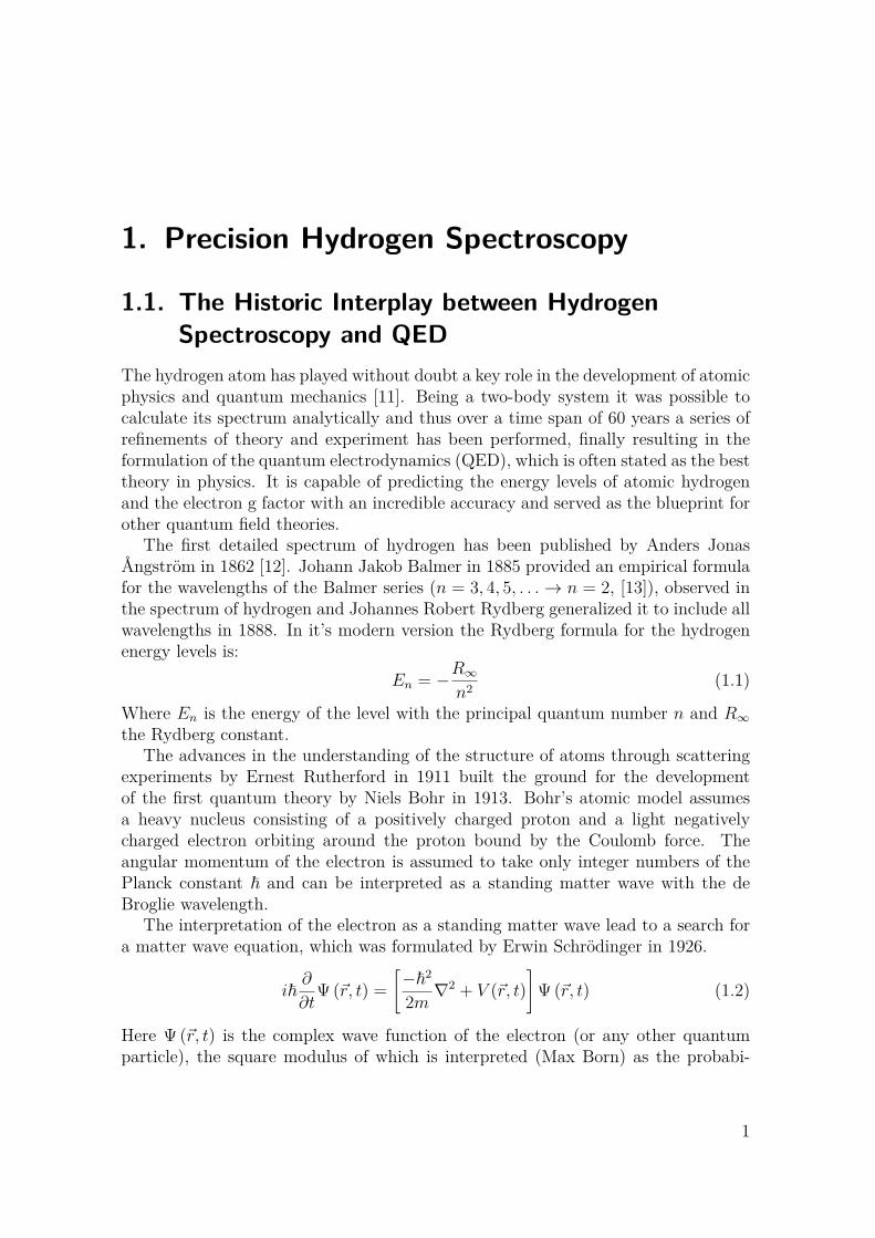
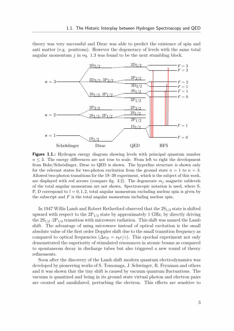
theory was very successful and Dirac was able to predict the existence of spin andanti matter (e.g. positrons). However the degeneracy of levels with the same totalangular momentum j in eq. 1.3 was found to be the next stumbling block.
Schrödinger Dirac QED HFS
n = 1
n = 3
3S1/2, 3P1/2
3D3/2, 3P3/2
3D5/23D5/2
3D3/23S1/2
1S1/2
1S1/2
F = 3
F = 1F = 1
F = 1
F = 2
F = 0
F = 0
3P3/2
3P1/2
n = 2
2P3/2 2P3/2
2S1/2, 2P1/22P1/2
2S1/2
F = 2
Figure 1.1.: Hydrogen energy diagram showing levels with principal quantum numbern ≤ 3. The energy differences are not true to scale. From left to right the developmentfrom Bohr/Schrödinger, Dirac to QED is shown. The hyperfine structure is shown onlyfor the relevant states for two-photon excitation from the ground state n = 1 to n = 3.Allowed two-photon transitions for the 1S–3S experiment, which is the subject of this work,are displayed with red arrows (compare fig. 3.2). The degenerate mj magnetic sublevelsof the total angular momentum are not shown. Spectroscopic notation is used, where S,P, D correspond to l = 0, 1, 2, total angular momentum excluding nuclear spin is given bythe subscript and F is the total angular momentum including nuclear spin.
In 1947 Willis Lamb and Robert Retherford observed that the 2S1/2 state is shiftedupward with respect to the 2P1/2 state by approximately 1 GHz, by directly drivingthe 2S1/2–2P1/2 transition with microwave radiation. This shift was named the Lambshift. The advantage of using microwave instead of optical excitation is the smallabsolute value of the first order Doppler shift due to the small transition frequency ascompared to optical frequencies (∆νD = ν0v/c). This epochal experiment not onlydemonstrated the superiority of stimulated resonances in atomic beams as comparedto spontaneous decay in discharge tubes but also triggered a new round of theoryrefinements.
Soon after the discovery of the Lamb shift modern quantum electrodynamics wasdeveloped by pioneering works of S. Tomonaga, J. Schwinger, R. Feynman and othersand it was shown that the tiny shift is caused by vacuum quantum fluctuations. Thevacuum is quantized and being in its ground state virtual photon and electron pairsare created and annihilated, perturbing the electron. This effects are sensitive to
3
1. Precision Hydrogen Spectroscopy
different electronic wave functions due to their different spatial distributions. QEDhas survived since than for over 70 years and more than six orders of magnitudeimprovement of experimental precision. Until today precision hydrogen spectroscopyremains a key tool for testing QED and determining the fundamental constants suchas the Rydberg constant or the root-mean square proton charge radius. New excitingproblems such as the proton radius puzzle, which will be discussed in the next section,make possible that new fundamental discrepancies could be found and shed light onthe most fundamental laws of nature.
Figure 1.1 summarizes the level structure within the different models, spanningabout 60 years of the development of QED. The energy differences are not true toscale. From left to right the historic development from Bohr/Schrödinger, Dirac toQED is shown. The hyperfine structure levels are displayed only for the relevantstates for two-photon excitation from the ground state n = 1 to n = 3. Allowedtwo-photon transitions for the 1S–3S experiment, which is the subject of this work,are displayed with red arrows. The degenerate mj magnetic sub-levels of the totalangular momentum are not shown. Spectroscopic notation is employed, where S, P,D correspond to l = 0, 1, 2, total angular momentum excluding nuclear spin is givenby the subscript and F is the total angular momentum including nuclear spin.
4
1.2. QED Description of the Energy Levels in Hydrogen
1.2. QED Description of the Energy Levels inHydrogen
While the simple Bohr model only needs the Rydberg constant R∞ to convert atomicunits into SI units for the energy equation 1.1 , including other effects such as rela-tivistic effects, recoil effects, QED vacuum fluctuations effects, finite proton chargedistribution etc., obviously complicate the energy relation and require knowledge ofadditional constants, such as the fine- structure constant α, the electron to protonmass ratio me/mp and the root-mean square (RMS) proton charge radius rp. At alevel of accuracy, which is not reached currently by experiment, also other constantssuch as the ratio of the electrons mass to Planck’s constant me/h would enter. Thefull description of the terms can be found in [4]. We restrict our self to the gene-ral formula, showing only the main Bohr/Schrödinger contribution, the QED seriesfn,`,j(α, memp , . . .) in the fine structure constant α and separately the finite proton sizecontribution. The resulting simplified formula for the QED energy levels of atomichydrogen reads:
En,`,j = R∞
(− 1n2 + fn,`,j(α,
me
mp
, . . .) + δ`,0CNSn3 r2
p
)(1.4)
with n, ` and j being the principle quantum number, and the orbital and totalangular momentum, respectively.
In principle, to fit N unknown parameters from the relation 1.4 (fundamentalconstants), one only needs to measure N transitions. By observing the residualsbetween the model 1.4 and the measurement using the best fit parameters, one canalready judge about the correctness of the model. With any additional independentmeasurement the model would be stronger restricted and possible statistically signi-ficant discrepancies would need to be attributed to either experimental or calculationerrors or to limitations of the theory itself. In principle the quantum electrodyna-mics could be falsified this way. It turns out that hydrogen spectroscopy is best indetermining only two of the four relevant constants, namely, the Rydberg constantR∞ and the RMS proton charge radius rp. Two other constants are determinedfrom other experiments, where they not merely enter as small contributions, but inleading order effects. The fine structure constant is determined from precision mea-surements of the electron g-factor [1] and the electron to proton mass ration me/mp
is determined from Penning trap experiments [2]. It is therefore of fundamentalscientific interest to measure more transitions and repeat measurements improvinguncertainties.
5
1. Precision Hydrogen Spectroscopy
1.3. Proton Radius PuzzleWe consider the finite proton charge radius correction in eq. 1.4. The proton (nuc-leus) is not a point–like particle, but rather its charge has a spherically symmetricdistribution with the root mean squared radius rp. Thus, the electron sees a reducedpotential and the energy levels are therefore slightly different than for the Coulombpotential (for the simple model of a homogeneously charged sphere, the potential isdifferent from the Coulomb potential only inside the charged sphere). Here, we areinterested to show the scaling of this energy correction with the mass of the particle(electron, muon) and the principal quantum number n. An illustrative calculationusing the simple model of a homogeneously charged sphere can be found in [15]. Thedifference potential W (r) between the coulomb potential of a point–like particle andthe potential of the charge distribution can be considered as perturbation and itseffect on the energy levels can be calculated in first order perturbation theory. Theenergy shifts in first order perturbation theory are simply the expectation value ofthe perturbation potential in the corresponding eigenstates. Since the potential isspherically symmetric the angular part of the wave function Y m∗
l (φ, θ)Y ml (φ, θ) just
integrates to one and we are left with:
∆En,l,m = 〈ψn,l,m|W |ψn,l,m〉 =∫ ∞
0R∗n,l(r)Rn,l(r)W (r)dr (1.5)
WhereRn,l(r) is the radial part of the hydrogen eigenstate |ψn,l,m〉. The characteristicextent of the electrons wave function is the Bohr radius a0 = ε0h
2/πmee2 ≈ 0.5 Å,
which is five orders of magnitude larger than the RMS proton charge radius rp ≈ 1 fm.Thus the radial part of the wave function in eq. 1.5 can be approximated by its valueat the origin Rn,l(0), which is nonzero only for s–states (l = 0). Thus we obtain:
∆En,l,m = |Rn,l(0)|2 δl0∫ ∞
0W (r)dr ∝ 1/n3a3
0 (1.6)
In other words the finite proton charge radius correction is proportional to the proba-bility density of the electron (muon) to be at the origin. For s–states the probabilitydensity at the origin is inversely proportional to the cube of the principal quantumnumber and the Bohr radius |Rn,l(0)|2 ∝ 1/n3a3
0. The mass of the muon and thus itsBohr radius a0 = ε0h
2/πmµe2 is 200–times smaller than for the electron. Therefore
the finite proton charge radius correction in muonic hydrogen is 2003 ≈ 107 sevenorders of magnitude larger than in ordinary hydrogen (also the absolute frequencyfor a given transition is ≈ 200 times larger). A new intriguing problem arose fromprecision spectroscopy of the muonic hydrogen in 2010 and attracted broad interest.It was coined the the Proton Radius Puzzle (PRP). The measurement of the Lambshift (2S–2P transition) in muonic hydrogen [3] determined the proton charge radiusto be 4 combined standard deviations smaller than the value determined from theregular atomic hydrogen. Taking into account the scattering data the discrepancy isdetermined in the global adjustment of fundamental constants [4] by the Committee
6
1.3. Proton Radius Puzzle
− % $ ' " #
& " ! −
# $
' " #
( # " ! $ % ! % ∞
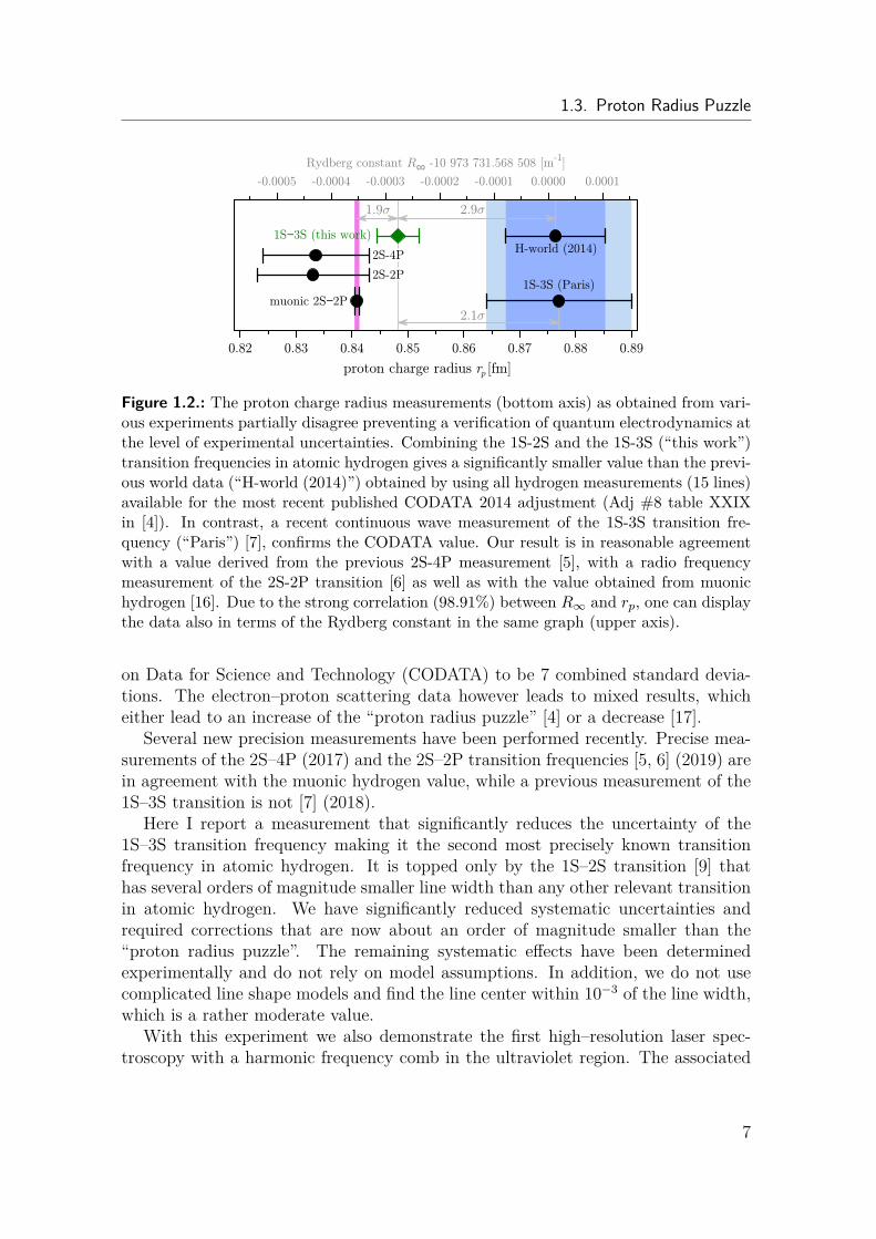
Figure 1.2.: The proton charge radius measurements (bottom axis) as obtained from vari-ous experiments partially disagree preventing a verification of quantum electrodynamics atthe level of experimental uncertainties. Combining the 1S-2S and the 1S-3S (“this work”)transition frequencies in atomic hydrogen gives a significantly smaller value than the previ-ous world data (“H-world (2014)”) obtained by using all hydrogen measurements (15 lines)available for the most recent published CODATA 2014 adjustment (Adj #8 table XXIXin [4]). In contrast, a recent continuous wave measurement of the 1S-3S transition fre-quency (“Paris”) [7], confirms the CODATA value. Our result is in reasonable agreementwith a value derived from the previous 2S-4P measurement [5], with a radio frequencymeasurement of the 2S-2P transition [6] as well as with the value obtained from muonichydrogen [16]. Due to the strong correlation (98.91%) between R∞ and rp, one can displaythe data also in terms of the Rydberg constant in the same graph (upper axis).
on Data for Science and Technology (CODATA) to be 7 combined standard devia-tions. The electron–proton scattering data however leads to mixed results, whicheither lead to an increase of the “proton radius puzzle” [4] or a decrease [17].
Several new precision measurements have been performed recently. Precise mea-surements of the 2S–4P (2017) and the 2S–2P transition frequencies [5, 6] (2019) arein agreement with the muonic hydrogen value, while a previous measurement of the1S–3S transition is not [7] (2018).
Here I report a measurement that significantly reduces the uncertainty of the1S–3S transition frequency making it the second most precisely known transitionfrequency in atomic hydrogen. It is topped only by the 1S–2S transition [9] thathas several orders of magnitude smaller line width than any other relevant transitionin atomic hydrogen. We have significantly reduced systematic uncertainties andrequired corrections that are now about an order of magnitude smaller than the“proton radius puzzle”. The remaining systematic effects have been determinedexperimentally and do not rely on model assumptions. In addition, we do not usecomplicated line shape models and find the line center within 10−3 of the line width,which is a rather moderate value.
With this experiment we also demonstrate the first high–resolution laser spec-troscopy with a harmonic frequency comb in the ultraviolet region. The associated
7
1. Precision Hydrogen Spectroscopy
short pulses help to avoid the photo–refractive effect in non–linear crystals that haslong hindered precision laser spectroscopy of the 1S–3S transition [18]. In the future,it may allow one to push the wavelengths to even shorter unexplored wavelength re-gions using high harmonic generation that hopefully will enable high resolution laserspectroscopy of hydrogen-like ions for the first time [19].
Combining the results for the 1S–3S and the 1S–2S transitions, we extract valuesfor the Rydberg constantR∞ and the RMS proton charge radius rp. These new valuesare two times more accurate than the ones obtained from all previous hydrogen datacombined. By using only two measurements to determine two constants/parameters,nothing can be said about the validity of QED. To check for consistency one needsadditional measurements. It does not matter whether we use the Rydberg constantor the RMS proton charge radius for this consistency check because the values ofthese parameters are strongly correlated through (1.4). In the current situationthis analysis yields mixed results. While this work favours the data from muonichydrogen and recently improved measurement of the 2S–2P Lamb shift in regularhydrogen [6], it deviates by 2.1σ from a recently published measurement of the 1S–3S transition frequency obtained by H. Fleurbaey and co-workers with a continuouslaser [7]. Further the RMS proton charge radius and the Rydberg constant, derivedfrom this measurement, are in very good agreement with the values derived from therecent measurement of the 2S–4P interval but disagrees by 2.9σ with the hydrogenworld data values evaluated by CODATA. Figure 1.2 summarises this situation.
8
1.4. Advances of the Garching 1S–3S Setup
1.4. Advances of the Garching 1S–3S SetupThe 1S–3S transition in hydrogen is very attractive for determination of the Rydbergconstant and the RMS proton charge radius and tests of QED for several reasons.First it is a two-photon transition and thus the first order Doppler shift is stronglysuppressed (see sections 5.1, 5.10). Second, it has a relatively small natural linewidth of only γ = 1.005 MHz. Besides the 1S–2S transition with several orders ofmagnitude smaller line width, only two-photon transitions to higher S and D states(2S–8S/8D for instance) possess even smaller natural line widths. However, thosetransitions are much more sensitive to DC Stark shifts due to the large spatial extentof the electronic wave function, which poses a serious experimental challenge. Quan-tum interference (compare section 5.8) is typically also a more important issue forthese transitions because of the dense level structure. On the contrary the DC Starkshift coefficient of the 1S–3S transition is only about 7 Hz(V/m)−2 (see section 5.5).Further, the low principal quantum numbers make the finite proton size correctionrelatively large.
The first precision measurement of the 1S–3S transition was performed in 2010by O. Arnoult in the group of F. Biraben at the Laboratoire Kastler Brossel (LKB)in Paris [20] with an uncertainty of 13 kHz. In 2016 our group at the Max-Planckinstitute of Quantum Optics performed a measurement with an uncertainty of 17 kHz[21]. In 2018 H. Fleurbaey from the LKB group performed an improved measurement[7] and combined with the previous measurement [20] obtained an uncertainty of2.6 kHz.
We should stress, that the 1S–3S transition is the only transition in hydrogen,which has been measured by two independent groups with sufficient low uncertaintyto contribute to the PSP and the constant determination. The groups use twodifferent techniques (continous wave vs. frequency comb, room temperature vs.cryogenic hydrogen) and thus have different leading systematic frequency shifts. Themeasurement presented in this work has an uncertainty of 0.72 kHz and differs inseveral aspects from previuos measurements. First it is the first 1S–3S transitionmeasurement performed with cryogenically cooled hydrogen atoms (T = 7 K), whichreduces the second order Doppler shift (SOD, see section 5.3) from roughly 120 kHzto 3 kHz. Second we could improve our laser system and the detection efficiencyto achieve a statistical uncertainty of 70 Hz only, which is more than one order ofmagnitude better than any previous result. With such a high signal strength wecould afford a direct measurement of all main systematic frequency shifts based onlinear interpolation and extrapolation in corresponding quantities (AC Stark shiftin power see section 5.2, CIFODS in chirp see section 5.1, pressure shift in atomicdensity, see section 5.4 and the SOD in temperature, see section 5.3). This is a veryreliable method since it does not depend on simulations since the nonlinearities inour case can be shown to be negligible. We believe that the present result can befurther improved.
9

2. Two-photon Direct Frequency CombSpectroscopy
2.1. Frequency Combs in Spectroscopy
Frequency combs have revolutionized the field of spectroscopy [22] and found nu-merous applications in other fields [23], [24]. For its invention T.W. Hänsch andJ.L. Hall were rewarded with a Nobel prize in physics in 2005 together with R.J.Glauber for his contributions to the theory of quantum optics. The broad spectrumof a frequency comb together with the regularly spaced mode structure serve as anoptical “ruler”, with which the high optical frequency of a spectroscopy laser canbe measured very precisely. Prior to frequency combs long phase locked frequencychains covering the whole range from radio frequency standards to the optical domainneeded to be built and operated.
Long before the ground breaking application of frequency combs for absolutefrequency determination they have been suggested for direct use in precision spec-troscopy experiments as the excitation source. E.V. Baklanov and V.P. Chebotaevsuggested in 1976 [25] to use frequency combs to drive the 1S–2S two-photon tran-sition in hydrogen. Contrary to one-photon transitions, where only one comb modecan be resonant with the transition, in a two-photon transitions all pairs of modeswhose frequencies add up to the transition frequency can contribute. The resul-ting excitation rate is the same as for an excitation with a continuous wave (CW)laser with the same average power. Further the line width of the transition is notbroadened by the large spectral width of the comb but rather is determined by thenarrow line width of the comb modes. Also the AC Stark shift is given by the aver-age intensity of the pulses rather than by the peak intensity [26]. This remarkablefeatures of the Direct Frequency Comb Spectroscopy have been soon after proposaldemonstrated by the group of T.W. Hänsch at Stanford in 1977 [27, 28] in a sodium3S–5S and 3S–4S transitions. The advantage of using frequency combs instead ofCW lasers is the high efficiency of pulsed lasers for nonlinear frequency conversionin crystals and gases. This opens the doors of precision spectroscopy in DUV andXUV regions, where no CW laser is available even today.
11
2. Two-photon Direct Frequency Comb Spectroscopy
2.2. Basics of Frequency CombsAs the name suggests an optical frequency comb is a regularly spaced array of laserfrequencies
ωn = nωr + ωCE (2.1)
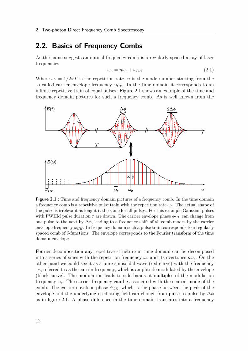
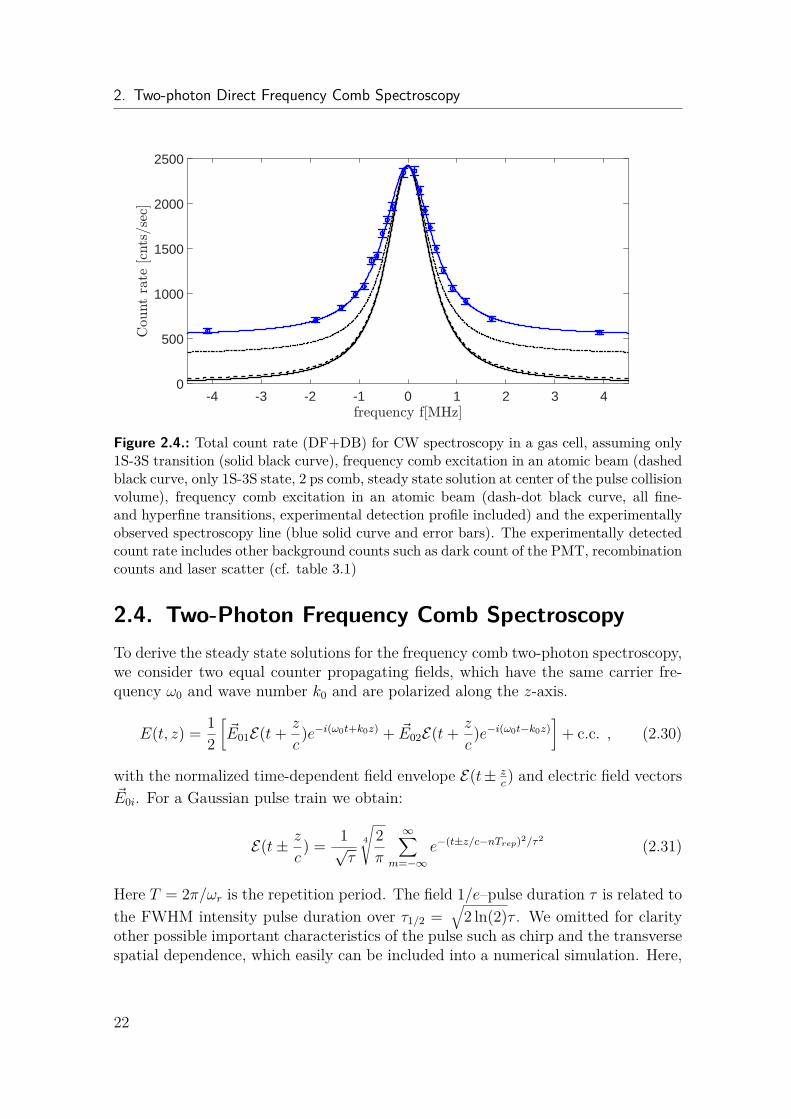
Where ωr = 1/2πT is the repetition rate, n is the mode number starting from theso called carrier envelope frequency ωCE. In the time domain it corresponds to aninfinite repetitive train of equal pulses. Figure 2.1 shows an example of the time andfrequency domain pictures for such a frequency comb. As is well known from the
Figure 2.1.: Time and frequency domain pictures of a frequency comb. In the time domaina frequency comb is a repetitive pulse train with the repetition rate ωr. The actual shape ofthe pulse is irrelevant as long it it the same for all pulses. For this example Gaussian pulseswith FWHM pulse duration τ are drawn. The carrier envelope phase φCE can change fromone pulse to the next by ∆φ, leading to a frequency shift of all comb modes by the carrierenvelope frequency ωCE . In frequency domain such a pulse train corresponds to a regularlyspaced comb of δ-functions. The envelope corresponds to the Fourier transform of the timedomain envelope.
Fourier decomposition any repetitive structure in time domain can be decomposedinto a series of sines with the repetition frequency ωr and its overtones nωr. On theother hand we could see it as a pure sinusoidal wave (red curve) with the frequencyω0, referred to as the carrier frequency, which is amplitude modulated by the envelope(black curve). The modulation leads to side bands at multiples of the modulationfrequency ωr. The carrier frequency can be associated with the central mode of thecomb. The carrier envelope phase φCE, which is the phase between the peak of theenvelope and the underlying oscillating field can change from pulse to pulse by ∆φas in figure 2.1. A phase difference in the time domain translates into a frequency
12
2.2. Basics of Frequency Combs
shift of all combs by the carrier envelope frequency ωCE = ∆φ/T . Experimentallya frequency comb can be realized by a mode-locked laser. In the laser resonatorthe pulse envelope propagates with the group velocity vg and the carrier with thephase velocity vp which are usually not equal due to the dispersion of the intra cavitymirrors, crystals or any other optical elements. Thus the pulse–to–pulse phase shiftbetween the envelope and the carrier is:
∆φ = ω0
(L
vg(ω0) −L
vp
)(2.2)
Generally the dispersion can be characterized by the frequency dependent wave num-ber k(ω), which can be decomposed into Tailor series around the central mode ω0.The round trip phase φn in the resonator of the mode ωn reads:
2L[k(ω0) + k
′(ω0)(ωn − ω0) + k′′(ω0)
2 (ωn − ω0)2 + h.o.
]= 2πn+ ∆φn (2.3)
where L is the length of the resonator. The phase difference between two neighboringmodes is given by:
k′(ω0)ωr + k
′′(ω0)2
[(ωn+1 − ω0)2 − (ωn − ω0)2
]+ h.o. = 2π + ∆φn+1 −∆φn
2L (2.4)
The first order derivative of the wave number with respect to ω (k′(ω0) = v−1g ) is
simply the inverse of the group velocity. The second order derivative k′′(ω) is thegroup velocity dispersion (GVD) (linear chirping), which makes the pulse envelopespread while it propagates. For a constant mode spacing the repetition rate ωrneeds to be independent on the mode number n. In eq. 2.4 this means that allterms, except of the first term k
′(ω0)ωr need to be zero for all mode numbers n,which is only possible if all derivatives of k(p)(ω0) vanish. Further the mode to modephase shift ∆φn+1−∆φn can not depend on n and thus must be a constant. In thisway the modes are “locked”. This remarkable property of mode–locked lasers can beverified by simply observing the spectrum of the pulses over time. A tiny deviationof 1 Hz would destroy the pulse after already 1 s. An observation of a constantpulse shape even after hours of operation demonstrates the vanishing of these terms.The width of the comb modes is in reality not a δ–function even for an infinitelylong pulse train. Phase noise and amplitude noise lead to a broadening of the combmodes. A detailed description of the frequency comb theory can be found in [29],written by one of the inventors of the frequency comb and my supervisor ThomasUdem.
13
2. Two-photon Direct Frequency Comb Spectroscopy
2.3. Continuous Wave Two-Photon SpectroscopyIn this section the basic theory of two-photon spectroscopy for one-photon forbiddendipole transitions is introduced for single frequency (CW) excitation. Based onthese general results, two-photon direct frequency comb spectroscopy is discussed inthe next section and differences between CW and frequency comb excitations arehighlighted.
For states with the same parity one-photon dipole transitions are forbidden andthe corresponding dipole moment matrix elements vanish, (e.g. for 1S–3S transition)
~de,g = 〈e| q~r |g〉 same parity= 0 (2.5)
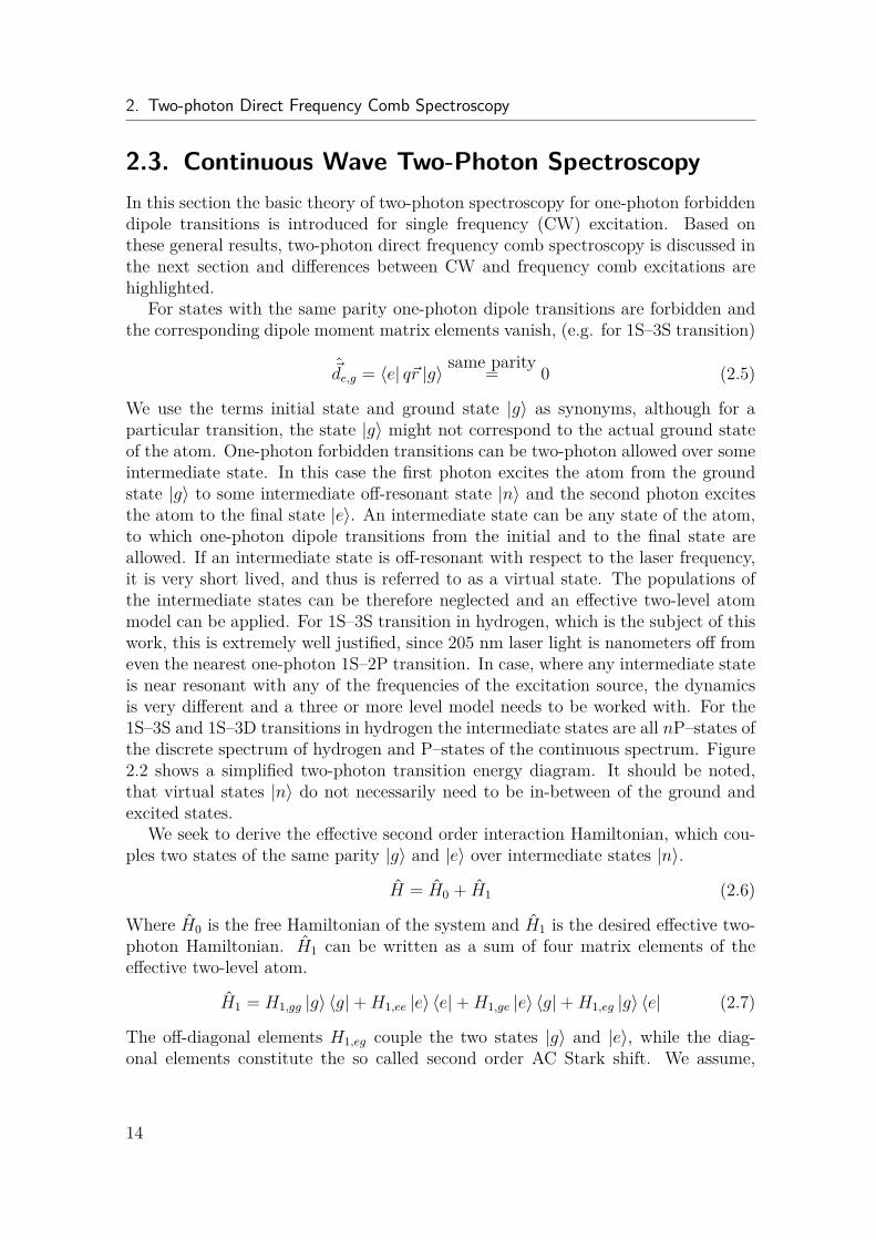
We use the terms initial state and ground state |g〉 as synonyms, although for aparticular transition, the state |g〉 might not correspond to the actual ground stateof the atom. One-photon forbidden transitions can be two-photon allowed over someintermediate state. In this case the first photon excites the atom from the groundstate |g〉 to some intermediate off-resonant state |n〉 and the second photon excitesthe atom to the final state |e〉. An intermediate state can be any state of the atom,to which one-photon dipole transitions from the initial and to the final state areallowed. If an intermediate state is off-resonant with respect to the laser frequency,it is very short lived, and thus is referred to as a virtual state. The populations ofthe intermediate states can be therefore neglected and an effective two-level atommodel can be applied. For 1S–3S transition in hydrogen, which is the subject of thiswork, this is extremely well justified, since 205 nm laser light is nanometers off fromeven the nearest one-photon 1S–2P transition. In case, where any intermediate stateis near resonant with any of the frequencies of the excitation source, the dynamicsis very different and a three or more level model needs to be worked with. For the1S–3S and 1S–3D transitions in hydrogen the intermediate states are all nP–states ofthe discrete spectrum of hydrogen and P–states of the continuous spectrum. Figure2.2 shows a simplified two-photon transition energy diagram. It should be noted,that virtual states |n〉 do not necessarily need to be in-between of the ground andexcited states.
We seek to derive the effective second order interaction Hamiltonian, which cou-ples two states of the same parity |g〉 and |e〉 over intermediate states |n〉.
H = H0 + H1 (2.6)
Where H0 is the free Hamiltonian of the system and H1 is the desired effective two-photon Hamiltonian. H1 can be written as a sum of four matrix elements of theeffective two-level atom.
H1 = H1,gg |g〉 〈g|+H1,ee |e〉 〈e|+H1,ge |e〉 〈g|+H1,eg |g〉 〈e| (2.7)
The off-diagonal elements H1,eg couple the two states |g〉 and |e〉, while the diag-onal elements constitute the so called second order AC Stark shift. We assume,
14
2.3. Continuous Wave Two-Photon Spectroscopy
Figure 2.2.: Two-photon excitation of a transition between two states |g〉, |e〉 with thesame parity and energies Eg and Ee over one-photon allowed off-resonant intermediatestates |n〉.
that the interaction is mediated by the dipole operator V (ε, t) = eELze−ε|t| cos(ωt),
which is a monochromatic plane wave, polarized in the z-direction and adiabaticallydamped at the distant past and future. The electric field is assumed to be con-stant within the atom (dipole approximation), which is a good approximation aslong as the wavelength λ is large compared to the typical size of the atom (Bohrradius). Analysis of the deviation from the dipole approximation can be found in[30]. The solution can be written as a superposition of the ground and excited states|ψ(t)〉 = e−iωgtcg(t) |g〉 + e−iωetce(t) |e〉. To calculate |ψ(t)〉 in second order pertur-bation theory, we transform the state |ψI(t)〉 = e−
i~ H0t |ψ〉 = cg(t) |g〉 + ce(t) |e〉
into the interaction picture and make use of the time evolution operator |ψI(t)〉 =UI(ε, t) |ψI(−∞)〉 = UI(ε, t) |g〉. The perturbation series for the time evolution ope-rator is given by the Dyson series.
UI(ε, t) = 1− i
~
t∫−∞
dt′VI(ε, t
′) +(− i~
)2 t∫−∞
dt′
t′∫
−∞
dt′′VI(ε, t
′)VI(ε, t′′) + . . . (2.8)
Where VI(ε, t) = ei~ H0tV (ε, t)e− i
~ H0t is the dipole potential in the interaction picture.When computing the matrix elements, the first order term vanishes, since bothstates |g〉 and |e〉 are parity eigenstates with the same eigenvalue and V (ε, t) ∝ r.We calculate the projection 〈φ|ψI(t)〉 of the state |ψI(t)〉 to some state |φ〉, where|φ〉 is either the ground state or the excited state.
M = 〈φ| UI(ε, t) |g〉 =(− i~
)2 t∫−∞
dt′
t′∫
−∞
dt′′ 〈φ| VI(ε, t
′)VI(ε, t′′) |g〉 (2.9)
We insert an identity operator and write the dipole interaction potential explicitly
15
2. Two-photon Direct Frequency Comb Spectroscopy
as a sum of exponentials.
M =(−ieEL2~
)2∑∫n,±
t∫−∞
dt′
t′∫
−∞
dt′′e±iω1t
′−ε|t′ |e±iω2t′′−ε|t′′ |×
〈φ| ei~H0t
′
ze−i~H0t
′
|n〉 〈n| ei~H0t
′′
ze−i~H0t
′′
|g〉
=(−ieEL2~
)2∑∫n,±
t∫−∞
dt′
t′∫
−∞
dt′′e±iω1t
′+iωφnt′−ε|t′ |e±iω2t
′′+iωngt′′−ε|t′′ | 〈φ| z |n〉 〈n| z |g〉
(2.10)
The ±-sum runs over all possible signs combinations of ω1 and ω2 in this equation(ω1 + ω2, −ω1 + ω2, ω1 − ω2, −ω1 − ω2), which we have denoted by introducing twodifferent frequencies ω1,2 to better keep track of the signs. Next, we evaluate theintegrals, where e−ε|t| assures the convergence. We further take the limit ε → 0,assuming long enough interaction time.
M(t) =(−ieEL2~
)2∑∫n,±
〈φ| z |n〉 〈n| z |g〉 ei(ωφg±ω1±ω2)t
[i(ωng ± ω2)] [i(ωφg ± ω1 ± ω2)] (2.11)
We are interested in the excitation probability Pφg from the ground state |g〉 to thefinal state |φ〉 in the time interval of t = −T/2 . . . T/2, which can be obtained usingthe Schrödinger equation H1,I |ψI(t)〉 = i~∂t |ψ(t)〉
Pφg =
∣∣∣∣∣∣∣T/2∫−T/2
〈φ| H1 |ψI(t)〉 dt
∣∣∣∣∣∣∣2
=
∣∣∣∣∣∣∣T/2∫−T/2
i~ 〈φ| ∂∂t|ψI〉 dt
∣∣∣∣∣∣∣2
=
∣∣∣∣∣∣∣T/2∫−T/2
i~∂
∂tM(t)dt
∣∣∣∣∣∣∣2
=
∣∣∣∣∣∣∣(eEL)2
4~∑∫n,±
〈φ| z |n〉 〈n| z |g〉ωng ± ω2
∣∣∣∣∣∣∣2 T/2∫−T/2
e−i(ωφg±ω1±ω2)tdt
︸ ︷︷ ︸→δ(ωφg±ω1±ω2), for T→∞
T/2∫−T/2
ei(ωφg±ω1±ω2)tdt
(2.12)
As expected, the excitation probability grows linearly and the excitation probabilityper unit time is a constant.
Pφg =
∣∣∣∣∣∣∣(eEL)2
4~∑∫n,±
〈φ| z |n〉 〈n| z |g〉ωng ± ω2
∣∣∣∣∣∣∣2
T (2.13)
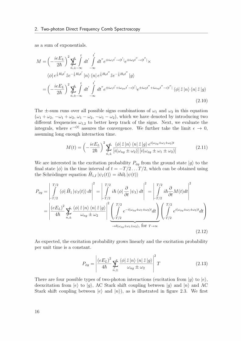
There are four possible types of two-photon interactions (excitation from |g〉 to |e〉,deexcitation from |e〉 to |g〉, AC Stark shift coupling between |g〉 and |n〉 and ACStark shift coupling between |e〉 and |n〉), as is illustrated in figure 2.3. We first
16
2.3. Continuous Wave Two-Photon Spectroscopy
Excitation Deexcitation AC Stark shift AC Stark shift
ω1
ω2
-ω1
-ω2 ω1 -ω2
-ω1 ω2
ω1 -ω2
-ω1 ω2
Figure 2.3.: The four possible two-photon interaction types are shown, corresponding to(de)exctitation and second order AC Stark shift of the ground and excited states, as givenby the different sign combinations in eq. 2.13
consider the probability for the atom to be excited from the ground state |g〉 tothe excited state |φ〉 = |e〉. The energy conservation in this case demands ωeg =ω1 + ω2 = 2ω. One can easily show, using the left part of the Schrödinger equationH1,I |ψI(t)〉 = i~∂t |ψ(t)〉, that the time-dependent off-diagonal matrix element ofthe two-photon dipole interaction Hamiltonian H1,eg, which satisfies equation 2.12,is given by the following expression.
H1,eg = e2
~∑∫n
〈e| z |n〉 〈n| z |φ〉ωng − ω
E(t)2 = 2(2πcε0)βegE(t)2 (2.14)
Note, that since (de)excitation requires the frequencies of the two photons to havethe same sign, the total two-photon matrix element is proportional to the square ofthe field E(t)2 and not the intensity I(t) ∝ E∗(t)E(t), as opposed to the AC Starkshift, which is discussed below. We have defined the time-independent two-photonmatrix element βeg [30].
βeg = e2
2hcε0∑∫n
〈e| z |n〉 〈n| z |φ〉ωng − ω
(2.15)
As explained above, the sum (integral for continuum states) in 2.15 runs over alleigenstates |n〉 of the free Hamiltonian of the system H0 with eigenenergies En andthe contribution of each intermediate level is given by its one-photon dipole elementswith the ground and excited states weighted by the laser frequency detuning from theintermediate transition (cf. fig. 2.2). βeg can be calculated using explicit expressionsfor the matrix elements of the discrete and continuum spectrum of hydrogen [31]and the eigenstates of the gross structure (quantum numbers n, l). Alternatively,one can use the explicit expressions for both discrete and continuum spectrum of theSturmian expansion [30]. Generally, for an arbitrary polarization, the two-photontransition operator can be written as following [30]
T ij = ri1
H0 − Eg − ~ωrj (2.16)
17
2. Two-photon Direct Frequency Comb Spectroscopy
Where ri represents any Cartesian coordinate. The eigenstates of the real hydrogenatom include fine- and hyperfine levels. Fortunately for S–S transitions, the two-photon operator has isotropic symmetry such that it transforms under rotation as ascalar. Thus βge for fine-structure and hyperfine structure can be obtained using theWigner-Eckart theorem, where n is the principal quantum number, S electron spin,L angular momentum, I nuclear spin, J = L + S and F = L + S + I total angularmomentum [30].
βge =− e2
4π~2cε0(−1)F
′−m′F
(F
′ 2 F−m′
f 0 mF
) √(2F + 1)(2F ′ + 1)×
(−1)J′+I+F+2
J
′F
′I
F J 2
√(2J + 1)(2J ′ + 1)×
(−1)L′+S+J+2
L
′J
′S
J L 2
× 〈n′
L′ | |T (2)| |nL〉
(2.17)
With this equations βeg can be calculated for any hyper-fine level and any polari-zation of the electric field. The 3j and 6j symbols are defined in [32]. For sometransitions and certain polarizations βge is zero and thus the transition is forbid-den. The resulting selection rules for two-photon dipole transitions are discussed in[33],[34].
Next, we consider the AC Stark shift case, in which the atom is initially in theground or excited state |φ〉 = |g〉 , |e〉 (S-state) then excited to any of the inter-mediate P-states |n〉 and then back to the |φ〉 (see fig. 2.2). Thus the energyconservation demands ω1 = −ω2 and we obtain from the equation 2.13.
∆EφAC ≡ H1,φφ = e2
~∑∫n,±
〈φ| z |n〉 〈n| z |φ〉ωng ± ω
E∗(t)E(t)︸ ︷︷ ︸2I(t)cε0
(2.18)
There is an important difference to the two-photon diagonal element in eq. 2.14. Asexplained above, the two photons have frequencies with opposite signs (first excitedthen deexcited or vice versa), such that the total matrix element is proportional tothe intensity of the field rather than the square. Summing up the AC Stark shift ofthe ground and excited states, the total transition frequency is shifted by:
δνAC = 1h
(∆EeAC(t)−∆Eg
AC(t)) = (βAC(e)− βAC(g)) I(t) (2.19)
Where we βAC(φ) is defined analogue to βeg as following and is calculated and ta-bulated for S-S-transition in hydrogen in [30].
βAC(φ) = − 4πe2
cε0h2
∑∫n,±
〈φ| z |n〉 〈n| z |φ〉ωng ± ω
(2.20)
18
2.3. Continuous Wave Two-Photon Spectroscopy
The second order AC Stark shift is proportional to the intensity ∝ I. The fourthorder of the AC Stark shift, which is proportional to the square of the intensity ∝ I2,is calculated in section B.
So far only one field has been assumed. The presented results can be immediatelyextended to the case of two-counter propagating fields with angular frequencies ω1,2and wave numbers k1,2, which are polarized along the z-axis.
E(t, z) = E1(t, z) + E2(t, z) = 12[E01e
−i(ω1t+k1z) + E02e−i(ω2t−k2z)
]+ c.c. (2.21)
The total Hamiltonian H is given by the following expression.
H = [~ωg + ∆EgAC(t)] |g〉 〈g|+ [~ωe + ∆Ee
AC(t)] |e〉 〈e|+ ~Ω(t)2 (|e〉 〈g|+ |g〉 〈e|)
(2.22)This is the same Hamiltonian as the two-level atom one-photon dipole interaction,except that the one-photon Rabi frequency is replaced by the two-photon Rabi fre-quency Ω(t).
Ω(t) = 2(2πcε0βge)E(t, z)2 = 2(2πcε0βge)
E1(t, z)2 + E2(t, z)2︸ ︷︷ ︸Doppler broadened
+ 2E1(t, z)E2(t, z)︸ ︷︷ ︸Doppler free
(2.23)
If the two beams are coming from the same laser and are counter propagating (k1 =−k2), then the product E1E2 is Doppler free. However different deviations can occur.For instance the wave vectors ~k1, ~k2 might be not perfectly anti parallel within theentire excitation volume, such that some residual Doppler shift occurs. We refer toit as “tilted wave front Doppler shift” (see. section 5.10). Note, that in the case of alinearly chirped frequency comb, the product of the fields has a position dependentparabolic phase along the pulse collision volume, which leads to an important combspectroscopy specific systematic residual first order Doppler-shift (see section 5.1).
Finally, just as in the one-photon case, we can derive the optical Bloch equa-tions, describing the population dynamics of the two levels. To this end we use theHamiltonian 2.22 and the Von Neumann equation for the density operator ρ.
i~dρ
dt=[H(t), ρ
]+ i~Γ(ρ) (2.24)
Where Γ(ρ) is the Lindblad operator, which describes the decay terms. The resultingset of differential equations is given in section 2.5, eq. 2.43, where the Monte Carlosimulation procedure is explained, which has been realized by Arthur Matveev [35]and used throughout the whole work on this experiment, to understand and verifythe different aspects of the experiment.
It is instructive to calculate the steady-state solutions for a CW laser from theoptical Bloch equations 2.43. Since the equations are linear the frequency comb case
19
2. Two-photon Direct Frequency Comb Spectroscopy
can be constructed from it as a sum of resonant pairs of comb modes. To this endwe set the derivatives in eq. 2.43 to zero and obtain the following solution.
RDFCW = Γρee = ΓΩ2/4
(ωeg − 2ω)2 + Γ2/4 + Ω2/2 ≈ΓΩ2/4
(ωeg − 2ω)2 + Γ2/4 (2.25)
In the last step Ω2/2 can be neglected in the denominator, if the Rabi frequencyΩ = 2(2πε0c)βgeE2
0 is much smaller than the natural line width Γ (for 1S–3S, 80 µm,0.1 W per direction, Ω = 625 Hz Γ = 2π × 1.005 MHz). Care must be takenwhen deriving the steady state solution as it is, strictly speaking, only valid for veryslow atoms, which propagate only a small distance within the life time of the excitedstate 1/(2πΓ). In this case the transverse and longitudinal position dependence ofthe fields can be neglected (but not the standing wave). As expected the steady statesolution is a Lorentzian line. RDF
CW = Γρee is the Doppler free (DF) count rate, i.e. thenumber of photons per unit of time per atom emitted when the atom decays to theground state. As expected the count rate is proportional to the intensity squaredΩ2 ∝ I2, which is due to the two-photon nature of the transition. The detuning∆ω = 2ω − ωeg is the difference between the resonance frequency ωeg and twice thelaser frequency ω. For a laser power of 0.1 W and 80µm waist (Γ = 1.005 MHz,1S–3S) the count rate is RCW ≈ 10−8 photons/atom sec. To be more precise, Γρeeis the probability of the decay to the ground state per atom per unit of time, sincethe semi-classical description does not include photons (second quantization). Tocalculate the experimentally observed count rate, the total number of atoms as wellas the collection efficiency and quantum efficiency of the detector must be known.
The excitation can also be driven by two photons from the same field. In thiscase ~k1 = ~k2 and the atom sees the Doppler shifted frequency 2ω ± 2kvz.
RDBCW = 1
4
[ΓΩ2/4
(ωeg − 2ω + 2kvz)2 + Γ2/4 + ΓΩ2/4(ωeg − 2ω − 2kvz)2 + Γ2/4
](2.26)
There are two Doppler broadened (DB) components, one from each direction of thefield. The Doppler-broadened lines are shifted by 2kvz and to obtain the full lineshape, one needs to integrate the expressions 2.26 over the velocity distribution p(v).In a gas cell (GC), where all directions are equally probable, the average velocity iszero. Both DB components are thus centered at the resonance frequency, just as theDF line. To obtain the Doppler broadened line shape, we can treat the Lorentzianlines for each velocity class as a delta function, since it is much narrower than theDoppler broadening.
RDBCW,GC =
∞∫−∞
12
2πΓΩ2/4Γ δ (∆ω ± 2kvz)
1√πvp
e−v2z/v
2pdvz
=√π
4Ω2
vpke−∆ω2/(4k2v2
p)
(2.27)
20
2.3. Continuous Wave Two-Photon Spectroscopy
Where ∆ω is the detunig from the resonance frequency, vp =√
2kBT/M is the mostprobable velocity (T temperature, kB Boltzmann constant and M atomic mass) ofthe Maxwellian distribution p(v) ∝ v2e−v
2/v2p . The velocity distribution for a single
velocity component p(vz) = 1/(√πvp)e−v
2z/v
2p is normally distributed. As expected,
the DB line is Gaussian line with the amplitude reduced by the factor√πΓ/4kvp as
compared to a single velocity class DB line. The width of the Doppler broadened linefor the 1S–3S transition in hydrogen at T = 7 K is ωD = 2
√ln 2kvp ≈ 2π × 3 GHz.
Taking eq. 2.25 for the DF line, the contrast between the DF and DB count ratesin a gas cell is given by the following ratio (cf. [34]).
CGCCW = 4kvp√
πΓ (2.28)
For an experiment with an atomic beam (AB) the situation is quite different in thatthe average velocity in z-direction is nonzero. In this case there are two separateDB lines, centered at ±4kvp, symmetrically around the resonance frequency. Thissignificantly reduces the Doppler broadened count rate around the resonance an thusimproves the contrast. If the atomic beam is sufficiently collimated and collinear withthe laser beam, we can neglect the x-, y-components and set the z-component equalto the modulus of the velocity. The Maxwell velocity distribution for a diffusivebeam is p(v) ∝ v3
ze−v2/v2
p .
RDBCW,AB =
∑±
∞∫−∞
2πΓΩ2/44Γ δ (∆ω ± 2kvz)H(±∆ω) 2
v4p
v3ze−v2
z/v2pdvz
= πΩ2
4e−∆ω2/(4k2v2
p)∆ω3
8k4v4p
[H(∆ω)−H(−∆ω)](2.29)
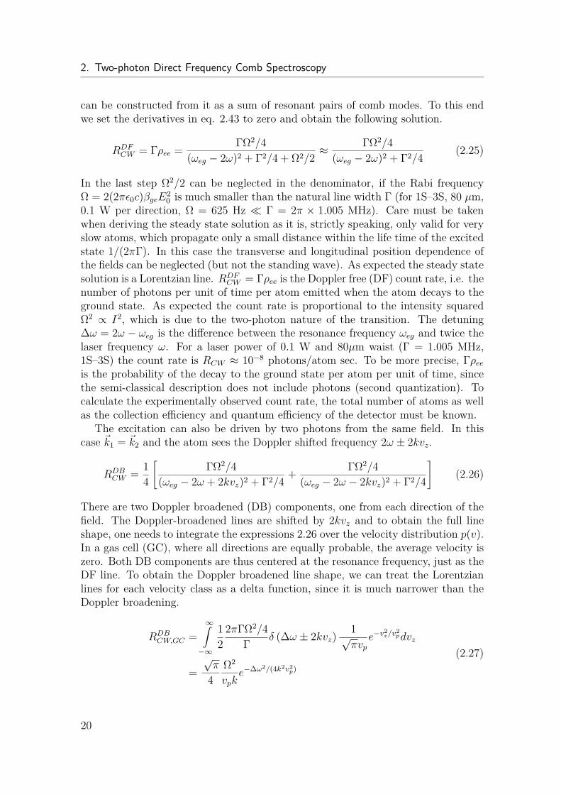
Where H(δω) is the Heaviside step function. To obtain the full Doppler broadenedcount rate, the polarization dependent excitation of the other fine- and hyperfinetransitions (1S-3S F = 0 and 1S-3D lines) has to be taken into account, since theDoppler width covers also these transitions. Therefore, the contrast generally isreduced. Figure 2.4 shows for comparison the expected total count rate (DF+DB)for CW spectroscopy in a gas cell, assuming only 1S-3S transition (solid black curve),frequency comb excitation in an atomic beam (dashed black curve, only 1S-3S state,2 ps comb, steady state solution), frequency comb excitation in an atomic beam(dash-dot black curve, all fine- and hyperfine transitions, experimental detectionprofile included) and the experimentally observed spectroscopy line (blue solid curveand error bars). Details to the contrast of the frequency comb spectroscopy areexplained in the next section and in chapter 3, table 3.1.
21
2. Two-photon Direct Frequency Comb Spectroscopy
frequency f[MHz]-4 -3 -2 -1 0 1 2 3 4
Count
rate
[cnts
/se
c]
0
500
1000
1500
2000
2500
Figure 2.4.: Total count rate (DF+DB) for CW spectroscopy in a gas cell, assuming only1S-3S transition (solid black curve), frequency comb excitation in an atomic beam (dashedblack curve, only 1S-3S state, 2 ps comb, steady state solution at center of the pulse collisionvolume), frequency comb excitation in an atomic beam (dash-dot black curve, all fine-and hyperfine transitions, experimental detection profile included) and the experimentallyobserved spectroscopy line (blue solid curve and error bars). The experimentally detectedcount rate includes other background counts such as dark count of the PMT, recombinationcounts and laser scatter (cf. table 3.1)
2.4. Two-Photon Frequency Comb SpectroscopyTo derive the steady state solutions for the frequency comb two-photon spectroscopy,we consider two equal counter propagating fields, which have the same carrier fre-quency ω0 and wave number k0 and are polarized along the z-axis.
E(t, z) = 12
[~E01E(t+ z
c)e−i(ω0t+k0z) + ~E02E(t+ z
c)e−i(ω0t−k0z)
]+ c.c. , (2.30)
with the normalized time-dependent field envelope E(t± zc) and electric field vectors
~E0i. For a Gaussian pulse train we obtain:
E(t± z
c) = 1√
τ4
√2π
∞∑m=−∞
e−(t±z/c−nTrep)2/τ2 (2.31)
Here T = 2π/ωr is the repetition period. The field 1/e–pulse duration τ is related tothe FWHM intensity pulse duration over τ1/2 =
√2 ln(2)τ . We omitted for clarity
other possible important characteristics of the pulse such as chirp and the transversespatial dependence, which easily can be included into a numerical simulation. Here,
22
2.4. Two-Photon Frequency Comb Spectroscopy
we are interested only in the general features of the solution. The Fourier transformof a Gaussian pulse envelope is given by the following expression.
E(mωr) =√τωr
4√2π
∞∑m=−∞
e−(mωrτ)2/4−imωrz/cδ(mωr) (2.32)
Thus the pulse train can be written as a sum of comb modes.
E(t, z) =E01√τωr
2 4√2π
∞∑m1=−∞
e−(m1ωrτ)2/4−i(ω0+m1ωr)t−ik0z−im1ωrz/c
+ E02√τωr
2 4√2π
∞∑m2=−∞
e−(m2ωrτ)2/4−i(ω0+m2ωr)t+ik0z−im2ωrz/c + c.c.(2.33)
Each pair of modes, which satisfies the resonance condition ωeg = 2ω0 +(m1 +m2)ωr,contributes to the excitation rate. Due to the periodicity of the frequency comb, thetransition will repeat itself for any multiple µωr of the repetition rate, however withreduced amplitude.
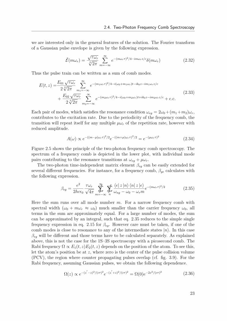
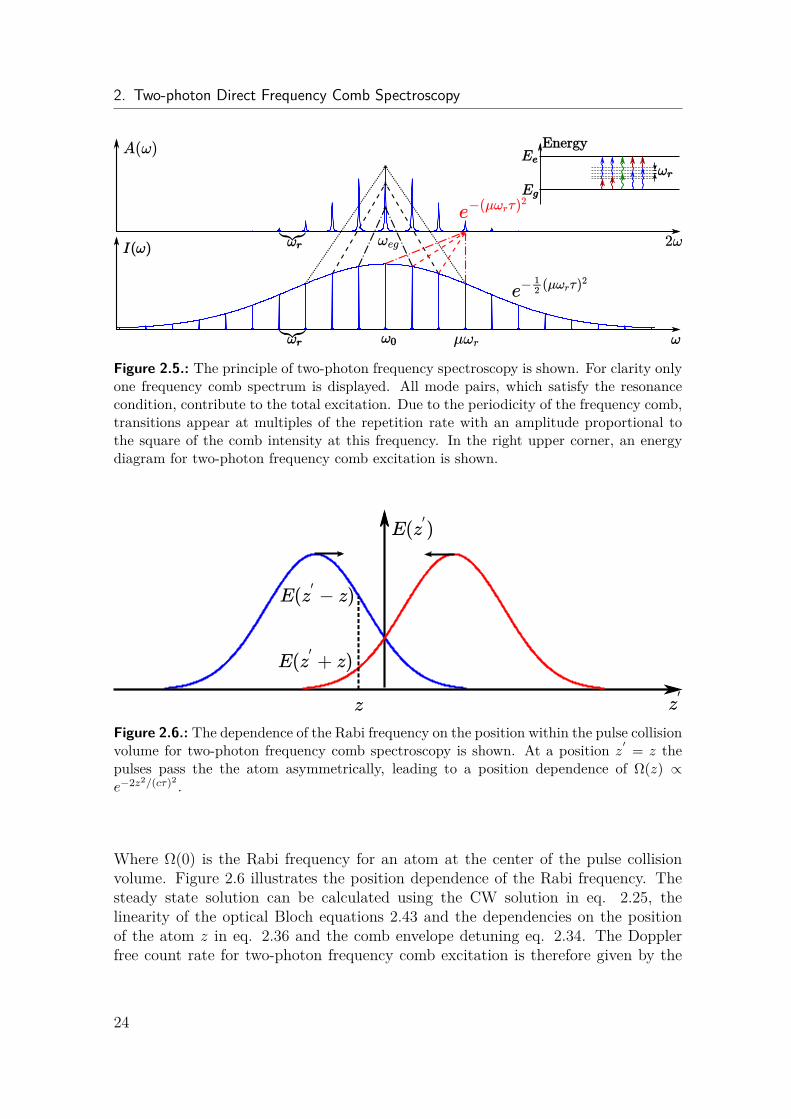
A(ω) ∝ e−((m−µ)ωrτ)2/2e−((m+µ)ωrτ)2/2 = e−(µωrτ)2 (2.34)
Figure 2.5 shows the principle of the two-photon frequency comb spectroscopy. Thespectrum of a frequency comb is depicted in the lower plot, with individual modepairs contributing to the resonance transitions at ωeg + µωr.
The two-photon time-independent matrix element βeg can be easily extended forseveral different frequencies. For instance, for a frequency comb, βge calculates withthe following expression.
βeg = e2
2hcε0τωr√
4π
∞∑∫m=−∞
∑∫n
〈e| z |n〉 〈n| z |e〉ωng − ω0 − ωrm
e−(mωrτ)2/2 (2.35)
Here the sum runs over all mode number m. For a narrow frequency comb withspectral width (ω0 + mωr ≈ ω0) much smaller than the carrier frequency ω0, allterms in the sum are approximately equal. For a large number of modes, the sumcan be approximated by an integral, such that eq. 2.35 reduces to the simple singlefrequency expression in eq. 2.15 for βeg. However care must be taken, if one of thecomb modes is close to resonance to any of the intermediate states |n〉. In this caseβeg will be different and those terms have to be calculated separately. As explainedabove, this is not the case for the 1S–3S spectroscopy with a picosecond comb. TheRabi frequency Ω ∝ E1(t, z)E2(t, z) depends on the position of the atom. To see this,let the atom’s position be at z, where zero is the center of the pulse collision volume(PCV), the region where counter propagating pulses overlap (cf. fig. 3.9). For theRabi frequency, assuming Gaussian pulses, we obtain the following dependence.
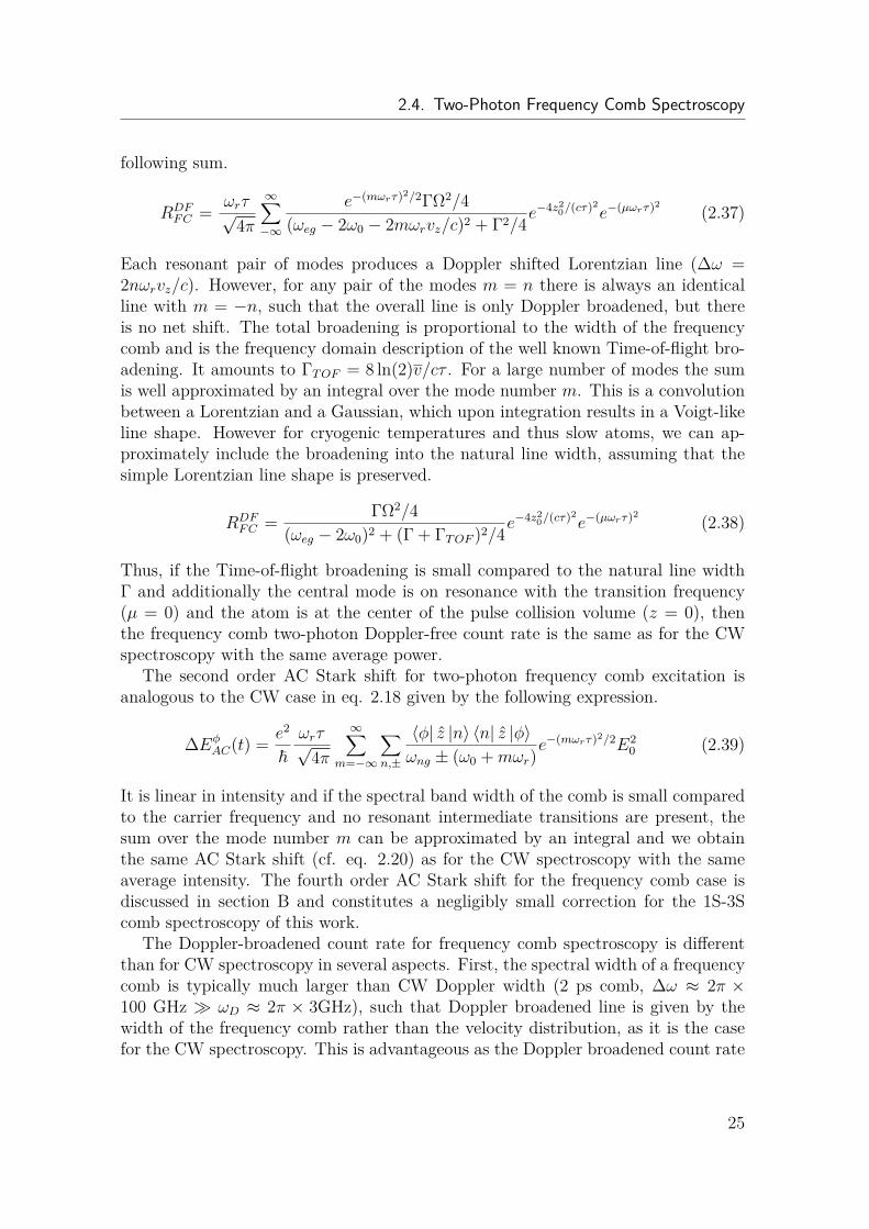
Ω(z) ∝ e−(z′−z)2/(cτ)2e−(z′+z)2/(cτ)2 = Ω(0)e−2z2/(cτ)2 (2.36)
23
2. Two-photon Direct Frequency Comb Spectroscopy
Figure 2.5.: The principle of two-photon frequency spectroscopy is shown. For clarity onlyone frequency comb spectrum is displayed. All mode pairs, which satisfy the resonancecondition, contribute to the total excitation. Due to the periodicity of the frequency comb,transitions appear at multiples of the repetition rate with an amplitude proportional tothe square of the comb intensity at this frequency. In the right upper corner, an energydiagram for two-photon frequency comb excitation is shown.
Figure 2.6.: The dependence of the Rabi frequency on the position within the pulse collisionvolume for two-photon frequency comb spectroscopy is shown. At a position z
′ = z thepulses pass the the atom asymmetrically, leading to a position dependence of Ω(z) ∝e−2z2/(cτ)2 .
Where Ω(0) is the Rabi frequency for an atom at the center of the pulse collisionvolume. Figure 2.6 illustrates the position dependence of the Rabi frequency. Thesteady state solution can be calculated using the CW solution in eq. 2.25, thelinearity of the optical Bloch equations 2.43 and the dependencies on the positionof the atom z in eq. 2.36 and the comb envelope detuning eq. 2.34. The Dopplerfree count rate for two-photon frequency comb excitation is therefore given by the
24
2.4. Two-Photon Frequency Comb Spectroscopy
following sum.
RDFFC = ωrτ√
4π
∞∑−∞
e−(mωrτ)2/2ΓΩ2/4(ωeg − 2ω0 − 2mωrvz/c)2 + Γ2/4e
−4z20/(cτ)2
e−(µωrτ)2 (2.37)
Each resonant pair of modes produces a Doppler shifted Lorentzian line (∆ω =2nωrvz/c). However, for any pair of the modes m = n there is always an identicalline with m = −n, such that the overall line is only Doppler broadened, but thereis no net shift. The total broadening is proportional to the width of the frequencycomb and is the frequency domain description of the well known Time-of-flight bro-adening. It amounts to ΓTOF = 8 ln(2)v/cτ . For a large number of modes the sumis well approximated by an integral over the mode number m. This is a convolutionbetween a Lorentzian and a Gaussian, which upon integration results in a Voigt-likeline shape. However for cryogenic temperatures and thus slow atoms, we can ap-proximately include the broadening into the natural line width, assuming that thesimple Lorentzian line shape is preserved.
RDFFC = ΓΩ2/4
(ωeg − 2ω0)2 + (Γ + ΓTOF )2/4e−4z2
0/(cτ)2e−(µωrτ)2 (2.38)
Thus, if the Time-of-flight broadening is small compared to the natural line widthΓ and additionally the central mode is on resonance with the transition frequency(µ = 0) and the atom is at the center of the pulse collision volume (z = 0), thenthe frequency comb two-photon Doppler-free count rate is the same as for the CWspectroscopy with the same average power.
The second order AC Stark shift for two-photon frequency comb excitation isanalogous to the CW case in eq. 2.18 given by the following expression.
∆EφAC(t) = e2
~ωrτ√
4π
∞∑m=−∞
∑n,±
〈φ| z |n〉 〈n| z |φ〉ωng ± (ω0 +mωr)
e−(mωrτ)2/2E20 (2.39)
It is linear in intensity and if the spectral band width of the comb is small comparedto the carrier frequency and no resonant intermediate transitions are present, thesum over the mode number m can be approximated by an integral and we obtainthe same AC Stark shift (cf. eq. 2.20) as for the CW spectroscopy with the sameaverage intensity. The fourth order AC Stark shift for the frequency comb case isdiscussed in section B and constitutes a negligibly small correction for the 1S-3Scomb spectroscopy of this work.
The Doppler-broadened count rate for frequency comb spectroscopy is differentthan for CW spectroscopy in several aspects. First, the spectral width of a frequencycomb is typically much larger than CW Doppler width (2 ps comb, ∆ω ≈ 2π ×100 GHz ωD ≈ 2π × 3GHz), such that Doppler broadened line is given by thewidth of the frequency comb rather than the velocity distribution, as it is the casefor the CW spectroscopy. This is advantageous as the Doppler broadened count rate
25
2. Two-photon Direct Frequency Comb Spectroscopy
is even less frequency dependent, reducing a possible asymmetric shift. Note, thatdue to the two-photon nature of the transition, the line width is proportional to thesquare of the intensity and thus the width of the comb reduces by a factor of
√2,
assuming a Gaussian comb. Second, each velocity class is excited by the frequencycomb as efficient as with the CW laser, but due to its large spectral width, a comb cansimultaneously talk to many velocity classes, thus increasing the Doppler-broadenedcount rate by approximately the number of modes within the spectral bandwidth2ωD/ωr (roughly 40 for 1S–3S transition). Therefore, the contrast of the Doppler-freeto Doppler-broadened count rates is approximately given by the following expression.
Ccomb = 4kvpΓ√π
ωr2ωD
= ωr
Γ√π ln(2)
(2.40)
As in the CW case this equation does not take into the account the polarizationdependent excitation of other allowed fine- and hyperfine components, which can alsobe resonant. Figure 2.4 shows the total theoretical and experimental line shapes ofthe 1S-3S transition in hydrogen for both CW and frequency comb excitation, whichincludes the polarization as well as detector properties (T = 7 K, main detector cf.section 3). Third, since the width of the Doppler broadened line is given by thespectral width of the comb, both DB lines from counter propagating beams will bealmost centered at the transition frequency, which is a disadvantage as comparedto the CW case, where the use of an atomic beam significantly reduces the Dopplerbackground and thus improves the contrast. Finally, as explained above, in the caseof frequency comb excitation, the Doppler-free fluorescence is emitted only within thetiny region, where the pulses overlap. The Doppler-broadened fluorescence is emittedacross the entire atomic beam and thus can be collected outside of the pulse collisionvolume using an independent detector. It than can be used as an almost perfectnormalization signal. This is explained in detail in section 4.2. This normalizationsignal is not present in the CW case, as the Doppler-free and Doppler-broadenedfluorescence can not be separated. In the next section, the Monte Carlo simulationfor the 1S–3S experiment is explained.
26
2.5. Monte Carlo simulations
2.5. Monte Carlo simulationsThe Monte Carlo simulation has been developed and performed by Arthur Matveev[35]. It has played a crucial role for the development and analysis of this experiment.The Monte Carlo simulation of the experimental 1S–3S line shapes consists of fourmodules. The first one determines a randomly picked atomic trajectory. The secondmodule solves the two–photon optical Bloch equations for an atom that flies alongthis trajectory through the pulse collision volume (PCV) for a certain laser detuning,intensity, pulse duration and chirp parameter. The third module determines thespatial fluorescence strength of the Balmer–α fluorescence, that is emitted uponthe 3S → 2P decay. The last module determines the line shape, by convolutingthe spatial fluorescence strength with the spatial light collection profiles of our fourdetectors (see section 3.6). To deal with different velocity distributions, we performthe computations for a set of velocities vj = 1 . . . 10, 000 m/s in j = 1 . . . 400 stepsof 25 m/s. A weighted sum allows us to use any velocity distribution model inpostprocessing the simulation results.
To seed the trajectories we first determine a starting point from a uniform dis-tribution on a circular surface within the nozzle that is perpendicular to the atomicand laser beam axis (the z–axis). This surface is not necessarily positioned at thenozzle orifice (see section 5.4). Adapted to the experimental set–up, the diameterof this surface is set to 1.5 mm. After the initial point is selected the angle of thetrajectory is drawn from a distribution that is proportional to cos(θ)dΩs [36], wheredΩs = | sin(θ)|dθdϕ and the polar and azimuthal angles θ and ϕ respectively. Thepolar angle is measured with respect to the beam axis. To accelerate a computation,the seeding algorithm checks if the trajectory passes through the PCV, and discardsthe trajectory if this is not the case. The condition is that it crosses an ellipsoidwith the semi–axis of 2w0 and 2cT1/2 that is centred at the PVC. We also save thefraction of trajectories that pass through the PCV for absolute calibration of thesignal. About 10,000 trajectories are used to sample the line at each of the 21 laserfrequencies that are used in the measurement. We use the same set of trajectoriesfor each laser frequency.
To test the dependence of the geometry we have varied the nozzle diameter andeven used an annual shape to model atoms that are directly emitted from the innersurfaces of the nozzle. We find very little variation of the resulting centre frequencieswith these alterations. The accuracy of the Monte Carlo simulation is given by thetypical variation of the centre frequencies between the trajectories divided by thesquare root of the number of trajectories. The variation is mostly determined by thevariation of AC–Stark shift, since the SOD is constant for a fixed velocity. Thereforewe can determine the line centres within a few Hz. We have verified this accuracyby comparing runs with different sets of trajectories. When comparing simulationswhere we artificially turn on and off some effects as described in section 5.11, weexpect an even smaller uncertainty, because the noise introduced through the choiceof the trajectories is common mode, at least when it is possible to compare runs with
27
2. Two-photon Direct Frequency Comb Spectroscopy
the same trajectory sets.Including collisions into the Monte Carlo simulation would be possible. Collisions
with large impact parameter (Weisskopf radius) lead to phase shifts and hence afrequency shift of the line, while the a small impact parameter resets the off–diagonalmatrix elements and leads to a collisional broadening (and possibly a new trajectory).To model all this would require two more random variables, the impact parameterand the relative velocity of the colliding atoms or molecules. In addition the chemicalcomposition, i.e. the hydrogen dissociation fraction depends on temperature (seefig.3.8). Hence including the pressure shift into our Monte Carlo simulation wouldsignificantly increase the computational effort that is already considerable. In lightof the smallness of the pressure shift we have not made an attempt in modelling itthis way.
To describe the evolution of the atomic state we use the optical Bloch equations(OBEs). In most of our simulations we represent the hydrogen atom as a two–levelsystem with the ground state g = |1S〉 and the excited state e = |3S〉. The OBEs fora two–photon transition are identical to the one–photon case, except that the Rabifrequency is computed differently. With the rotating wave approximation, they canbe expressed in terms of the density matrix:
ρgg = −iΩ∗(t)2 ρeg + i
Ω(t)2 ρge + Γρee (2.41)
ρge = −i∆ω ρge + iΩ∗(t)
2 (ρgg − ρee)−12Γρge (2.42)
ρee = +iΩ∗(t)2 ρeg − i
Ω(t)2 ρge − Γρee (2.43)
The equation for ρeg is obtained as the complex conjugate of the second equation.Here Ω(t) is the Rabi frequency that is given in (5.2) but deprived of the carrierfrequency −2ωc, because of the rotating wave approximation. For chirped pulsesthe Rabi frequency becomes complex in contrast to the two–photon OBEs in [30].The 3S → 2P decay rate is given by Γ/2π = 1.0050 MHz and the laser detuning by∆ω. Photoionization of the excited state is possible with just one additional laserphoton and might be included into the OBEs. However, for the power levels in use,this results in a sub–Hz line shift so that we ignore ionization here. The secondorder Doppler and AC–Stark (see (5.13)) shifts are readily included into the OBEsby subtracting them from the laser detuning:
∆ω = 2π (ν − ν0) + 2πν0v2
2c2 − δνAC (2.44)
As in (4.1), the laser frequency and the unperturbed transition frequency are givenby ν and ν0 respectively. In the simulations we usually set ν0 = 0, since we are onlyinterested in relative line shifts. After solving the OBEs as a function of time, thefluorescence signal emitted between tk and tk+1 computes as:
sk(ν, vj) = Γ∫ tk+1
tk
ρee(t)dt. (2.45)
28
2.5. Monte Carlo simulations
Knowing the position of the atom as a function of time, we can determine thespatial fluorescence strength. As sk(ν, vj) increases by unity for one decay event, theunit of sk(ν, vj) is photons, even though the semi–classical OBEs actually do notknow about photons. The Rabi frequency parameter βge is given in [30] for linearlaser polarisation. Converting to σ+ and σ− polarisations, this parameter becomesβge = −1.00333 × 10⁻⁵ Hz/(W/m2) and βge = −3.082895 × 10⁻⁵ Hz/(W/m2) forthe 1S–3S and 1S-3D transition respectively. The latter coefficient is has to bemultiplied by +1/2 relative the value given in [30]. The latter is required to modelthe quantum interference (see section 5.8), for which we need to expand the OBEsto include the D–levels, the final P–levels, their fine– and hyperfine structure aswell as all corresponding Zeeman levels. The resulting OBEs consist of 1600 coupleddifferential equations that are derived using a computer algebra system and numericalintegrated on a large scale cluster computer [35].
Since the laser beam radius near the PCV is much smaller than the depth offocus and the resolution of our light collection optics, we do not save the x and y–coordinates of the spatial fluorescence strength. Instead the integration code splitsthe integration interval from zk = −2 mm to zk = +2 mm into k = 1 . . . 400slices of 10 µm each. The times tk in (2.45) are the entrance times into the k–thslice of the trajectory under consideration. Finally, to obtain the simulated lineshapes as observed with the various detectors, we are convoluting the spatial lightcollection profiles pD(z) with the spatial fluorescence strength. We determine pD(z)with a Monte Carlo method by drawing a position within the PCV and an emissiondirection from an isotropic distribution. Following this ray determines whether or notit hits one of the light collecting lenses (see section 3.6). If it does, we compute therefraction through the lens and determine whether it ends up within the acceptancecone of the multi–mode fibre behind the lens. The light collection profiles obtainedin this way are shown in fig.3.10. Finally the simulated line shape is obtained via:
LMC(ν, z) =∑j,k
sk(ν, vj) p(vj) pD(zk − zD), (2.46)
where zD is the central position of the light collecting lens and p(vj) is the normalizedatomic velocity distribution. Examples for light collection profiles pD(z) and fittingresults to LMC(ν, z) are seen in fig.5.2.
29

3. Experimental setupIn this chapter the experimental setup is presented. Fig. 3.1 shows the generalscheme of the 1S–3S experiment. In the following sections the individual parts areexplained. In section 3.1 the absolute frequency determination is described (left sideof fig. 3.1). Section 3.2 deals with the frequency quadrupling to obtain 205 nmfrequency comb for spectroscopy and explains the chirp generation mechanism viaself-phase modulation process in the second harmonic generation cavities (right sidein fig. 3.1, compare fig. 3.3, 3.4,). In section 3.4 the vacuum system with theenhancement cavity and differential pumping to prevent mirror degradation are ex-plained (compare fig. 3.6, 3.6). Section 3.5 deals with the hydrogen discharge andthe liquid helium cryostat cooling (fig. 3.7, 3.8). Finally, section 3.6 presents thedetails of the fluorescence detection (fig. 3.9, 3.10).
3.1. Frequency measurementAs shown in Fig. 3.1, we operate two frequency combs at 820 nm – one generatedby a femtosecond laser (“fs-comb”) to determine the optical frequency of the 1S-3S transition, and one from a picosecond laser (“ps-comb”) for direct frequencycomb spectroscopy. The ps-comb is obtained with a mode-locked Ti:sapphire laser(Spectra Physics, Tsunami) and the fs-comb is generated with a frequency doubledmode-locked erbium-doped fiber laser (Menlo Systems, FC1500). The ps-comb iscalibrated by the fs-comb in two steps. First, we measure the reference frequencyof a continuous wave (cw) extended cavity diode laser (ECDL) at 820 nm that islocked to an ultra stable cavity with the Pound-Drever-Hall technique:
fref(820 nm) = (1 461 379× 250) MHz + 60 MHz− 150 MHz + 〈fb〉. (3.1)
The repetition and carrier-envelope offset frequencies of the fs-comb are set to250 MHz and 60 MHz respectively using a GPS disciplined hydrogen maser as areference. The calibration uncertainty contributes 30 Hz to the absolute frequency(see table 5.1). The 150 MHz frequency offset is obtained through mixers to obtainmore convenient frequencies for counting. The beat note frequency fb of the cw laserwith the 1 461 379-th mode of the fs-comb is recorded redundantly with two Λ-typecounters [51] (K+K Messtechnik, FX80), and is stable enough so that is treated as aconstant during a line scan that takes ≈ 36 sec. By using a line-scan-averaged value〈fb〉 we effectively remove residual noise of the hydrogen maser that is much largerthan the cavity-locked cw laser at this time scale. Without using the ultra stablecavity as a flywheel, the 1S-3S lines would look considerably more noisy.
31
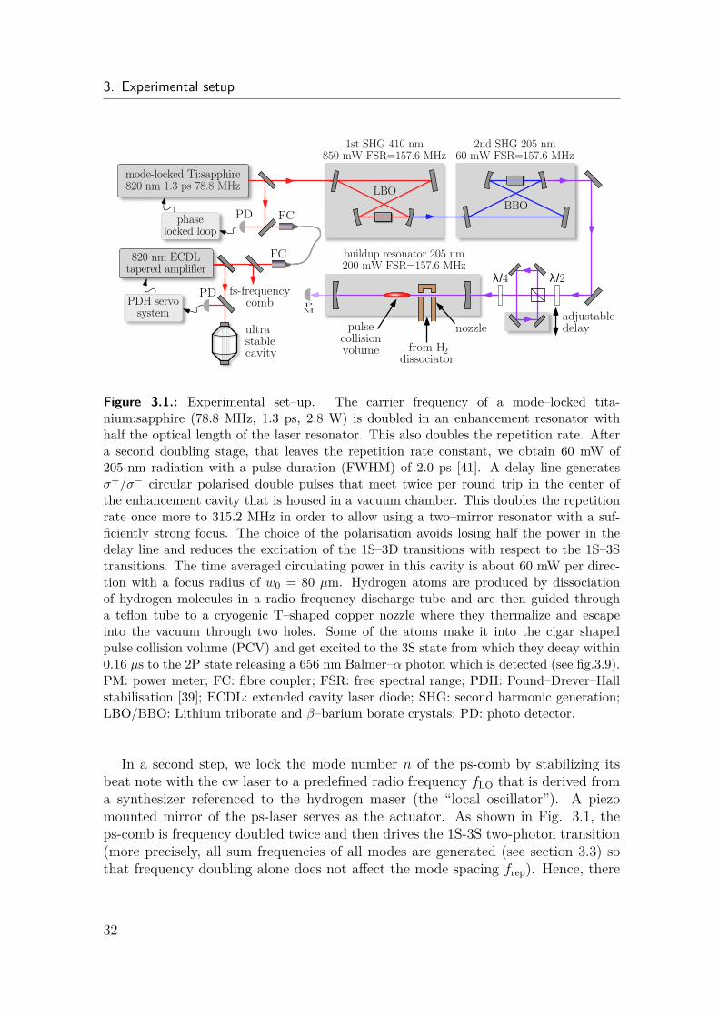
3. Experimental setup
1st SHG 410 nm850 mW FSR=157.6 MHz
2nd SHG 205 nm60 mW FSR=157.6 MHz
BBO
LBO
buildup resonator 205 nm200 mW FSR=157.6 MHz
λ/2λ/4
adjustabledelay
from Hdissociator
2
pulsecollisionvolume
mode-locked Ti:sapphire820 nm 1.3 ps 78.8 MHz
PDphaselocked loop
FC
FC
PDPDH servo
system
820 nm ECDLtapered amplifier
fs-frequencycomb
ultrastablecavity
nozzle
PM
Figure 3.1.: Experimental set–up. The carrier frequency of a mode–locked tita-nium:sapphire (78.8 MHz, 1.3 ps, 2.8 W) is doubled in an enhancement resonator withhalf the optical length of the laser resonator. This also doubles the repetition rate. Aftera second doubling stage, that leaves the repetition rate constant, we obtain 60 mW of205-nm radiation with a pulse duration (FWHM) of 2.0 ps [41]. A delay line generatesσ+/σ− circular polarised double pulses that meet twice per round trip in the center ofthe enhancement cavity that is housed in a vacuum chamber. This doubles the repetitionrate once more to 315.2 MHz in order to allow using a two–mirror resonator with a suf-ficiently strong focus. The choice of the polarisation avoids losing half the power in thedelay line and reduces the excitation of the 1S–3D transitions with respect to the 1S–3Stransitions. The time averaged circulating power in this cavity is about 60 mW per direc-tion with a focus radius of w0 = 80 µm. Hydrogen atoms are produced by dissociationof hydrogen molecules in a radio frequency discharge tube and are then guided througha teflon tube to a cryogenic T–shaped copper nozzle where they thermalize and escapeinto the vacuum through two holes. Some of the atoms make it into the cigar shapedpulse collision volume (PCV) and get excited to the 3S state from which they decay within0.16 µs to the 2P state releasing a 656 nm Balmer–α photon which is detected (see fig.3.9).PM: power meter; FC: fibre coupler; FSR: free spectral range; PDH: Pound–Drever–Hallstabilisation [39]; ECDL: extended cavity laser diode; SHG: second harmonic generation;LBO/BBO: Lithium triborate and β–barium borate crystals; PD: photo detector.
In a second step, we lock the mode number n of the ps-comb by stabilizing itsbeat note with the cw laser to a predefined radio frequency fLO that is derived froma synthesizer referenced to the hydrogen maser (the “local oscillator”). A piezomounted mirror of the ps-laser serves as the actuator. As shown in Fig. 3.1, theps-comb is frequency doubled twice and then drives the 1S-3S two-photon transition(more precisely, all sum frequencies of all modes are generated (see section 3.3) sothat frequency doubling alone does not affect the mode spacing frep). Hence, there
32
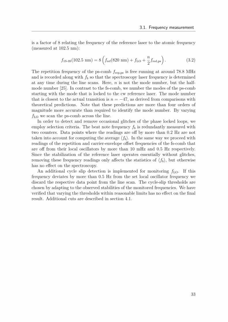
3.1. Frequency measurement
is a factor of 8 relating the frequency of the reference laser to the atomic frequency(measured at 102.5 nm):
f1S-3S(102.5 nm) = 8(fref(820 nm) + fLO + n
2 fred,ps
). (3.2)
The repetition frequency of the ps-comb frep,ps is free running at around 78.8 MHzand is recorded along with fb so that the spectroscopy laser frequency is determinedat any time during the line scans. Here, n is not the mode number, but the half-mode number [25]. In contrast to the fs-comb, we number the modes of the ps-combstarting with the mode that is locked to the cw reference laser. The mode numberthat is closest to the actual transition is n = −47, as derived from comparisons withtheoretical predictions. Note that these predictions are more than four orders ofmagnitude more accurate than required to identify the mode number. By varyingfLO we scan the ps-comb across the line.
In order to detect and remove occasional glitches of the phase locked loops, weemploy selection criteria. The beat note frequency fb is redundantly measured withtwo counters. Data points where the readings are off by more than 0.2 Hz are nottaken into account for computing the average 〈fb〉. In the same way we proceed withreadings of the repetition and carrier-envelope offset frequencies of the fs-comb thatare off from their local oscillators by more than 10 mHz and 0.5 Hz respectively.Since the stabilization of the reference laser operates essentially without glitches,removing these frequency readings only affects the statistics of 〈fb〉, but otherwisehas no effect on the spectroscopy.
An additional cycle slip detection is implemented for monitoring fLO. If thisfrequency deviates by more than 0.5 Hz from the set local oscillator frequency wediscard the respective data point from the line scan. The cycle-slip thresholds arechosen by adapting to the observed stabilities of the monitored frequencies. We haveverified that varying the thresholds within reasonable limits has no effect on the finalresult. Additional cuts are described in section 4.1.
33
3. Experimental setup
−
Figure 3.2.: Multiple 1S-3S/D two-photon transitions fold into the spectrum due to thefrequency comb so that the separation of the line components appear modulo ωr = 2π ×315.2 MHz. By operating a well chosen ωr and with circular polarization, we obtain awell-isolated 1S(F = 1)-3S(F = 1) component. Other components that are allowed bythe selection rules are a: 1S(F = 1)-3D5/2; b: 1S(F = 0)-3D3/2(F = 2); c: 1S(F = 0)-3D5/2(F = 2); d: 1S(F = 1)-3D3/2; e: 1S(F = 0)-3S(F = 0). The hyperfine splitting of the3D states is smaller than the natural line width and thus unresolved. The baseline offset isfrom the Doppler-broadened absorption of two co-propagating photons. The inset showsan average of 5 lines scans (3 min) within ±4 MHz of the main component, normalizedto the Doppler-broadened signal, together with a Lorentzian fit. The sampling of thefrequency axis was chosen to yield an approximately equidistant spacing on the signal axisin order to maximize the sensitivity to the center frequency per unit of measurement time.The line pulling by other 1S-3D lines and others (not visible) is negligible and discussed indetail in the supplement. The detuning in this graph is measured at the atomic frequency,i.e. around the frequency given in (6.1).
3.2. Laser systemThe laser system has been evolved only slightly since it has been described in detail[41]. Driving the 1S–3S Doppler free two–photon transition requires two counterpropagating photons at 205.145 nm, that are generated as the fourth harmonic intwo subsequent doubling cavities. With two–photon direct frequency comb spec-troscopy all fine– and hyperfine components are folded into the recorded spectrumwith modulo of half the mode spacing (repetition rate) of the comb. Fig. 3.2 showsand explains the resulting full frequency scan pattern.
To prevent other components from overlapping spectrally with the component ofinterest, it is desirable to operate at a sufficiently large repetition rate and to chooseits exact value wisely. The repetition rate of 78.8 MHz of our ps-laser is too lowfor this purpose. Conventional frequency doubling in nonlinear crystals does notdouble the repetition rate because this process actually generates sum frequencies
34
3.2. Laser system
of all possible combination of modes. Nevertheless, we can double the repetitionrate by employing an enhancement cavity with a free spectral range that is twicethe repetition rate of the ps-laser. Both of our doubling cavities have a free spectralrange of around 2 × 78.8 MHz = 157.6 MHz. As a result, we use only half of thelaser power (every second mode). As shown in Fig. 3.1, a combination of waveplates, beam splitters and a delay line generates σ± circular polarized double pulses,without further loss of laser power. This doubles the pulse repetition rate as seenby the atoms once more to frep = 4 × frep,ps = 315.2 MHz. This specific valueisolates the 1S(F =1)-3S(F =1) component to minimize line pullings, i.e. apparentshifts of the extracted center frequency of the main resonance due to the proximityof other resonances (see section 5.9). To obtain the real unfolded line separationof components a), b), c), d) and e) from Fig. 3.2, one needs to add 13, 14, 17, 9and 4 times 315.2 MHz respectively. To prevent other components from overlappingspectrally with the component of interest, it is desirable to operate at a sufficientlylarge repetition rate and to choose its exact value wisely. The repetition rate of78.8 MHz of our ps-laser is too low for this purpose. Conventional frequency doublingin nonlinear crystals does not double the repetition rate because this process actuallygenerates sum frequencies of all possible combination of modes. Nevertheless, we candouble the repetition rate by employing an enhancement cavity with a free spectralrange that is twice the repetition rate of the ps-laser. Both of our doubling cavitieshave a free spectral range of around 2 × 78.8 MHz = 157.6 MHz. As a result, weuse only half of the laser power (every second mode). As shown in Fig. 3.1, acombination of wave plates, beam splitters and a delay line generates σ± circularpolarized double pulses, without further loss of laser power. This doubles the pulserepetition rate as seen by the atoms once more to frep = 4×frep,ps = 315.2 MHz. Thisspecific value isolates the 1S(F =1)-3S(F =1) component to minimize line pullings,i.e. apparent shifts of the extracted center frequency of the main resonance due tothe proximity of other resonances (see section 5.9). To obtain the real unfolded lineseparation of components a), b), c), d) and e) from Fig. 3.2, one needs to add 13,14, 17, 9 and 4 times 315.2 MHz respectively.
The first frequency doubling stage uses a 5 mm long lithium triborate (LBO)crystal (cut at θ = 90, φ = 29.7). It is used within a four mirror bowtie ring cavitywith two curved mirrors (ROC = 210 mm, waist radius w0 = 40 µm). The inputpower from the laser is around 2.8 W and the single pass efficiency is around 5-10%,allowing for a low finesse cavity (input coupler transmission T = 30%). The typicaloutput power at the second harmonic is 800 mW which corresponds to an efficiencyof almost 60% for the laser modes that are actually used. One of the flat mirrors ismounted on a piezo transducer to stabilize the cavity with respect to the laser usingthe polarization method [52].
The second doubling stage uses the same type of four mirror ring cavity (ROC= 210 mm, waist w0 = 30 µm, T = 30%) with a 5 mm barium borate (BBO,θ = 85.7) crystal. The crystal is cooled to −20C to increase its conversion coefficient(deff = 0.318 pm/V) and is flushed with dry nitrogen during operation to prevent
35
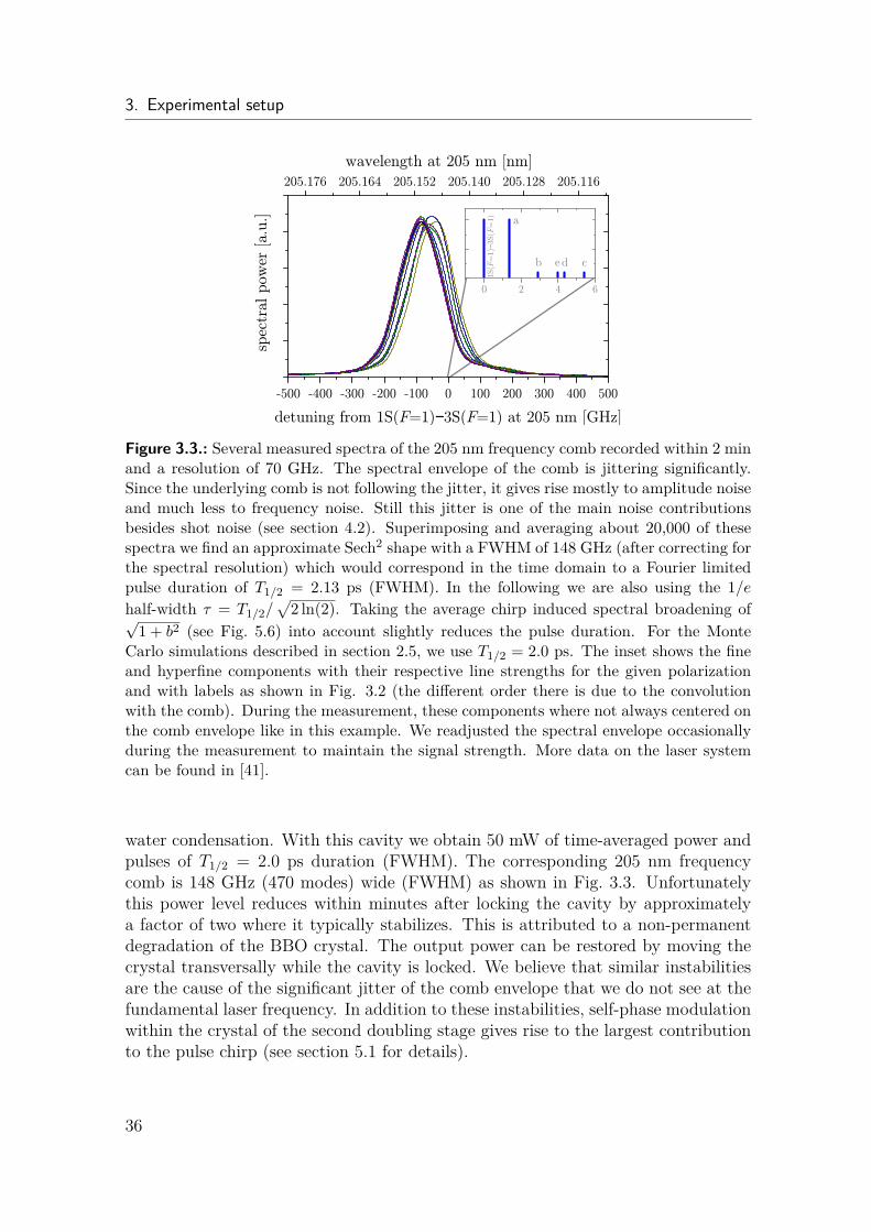
3. Experimental setup
−
−
Figure 3.3.: Several measured spectra of the 205 nm frequency comb recorded within 2 minand a resolution of 70 GHz. The spectral envelope of the comb is jittering significantly.Since the underlying comb is not following the jitter, it gives rise mostly to amplitude noiseand much less to frequency noise. Still this jitter is one of the main noise contributionsbesides shot noise (see section 4.2). Superimposing and averaging about 20,000 of thesespectra we find an approximate Sech2 shape with a FWHM of 148 GHz (after correcting forthe spectral resolution) which would correspond in the time domain to a Fourier limitedpulse duration of T1/2 = 2.13 ps (FWHM). In the following we are also using the 1/ehalf-width τ = T1/2/
√2 ln(2). Taking the average chirp induced spectral broadening of√
1 + b2 (see Fig. 5.6) into account slightly reduces the pulse duration. For the MonteCarlo simulations described in section 2.5, we use T1/2 = 2.0 ps. The inset shows the fineand hyperfine components with their respective line strengths for the given polarizationand with labels as shown in Fig. 3.2 (the different order there is due to the convolutionwith the comb). During the measurement, these components where not always centered onthe comb envelope like in this example. We readjusted the spectral envelope occasionallyduring the measurement to maintain the signal strength. More data on the laser systemcan be found in [41].
water condensation. With this cavity we obtain 50 mW of time-averaged power andpulses of T1/2 = 2.0 ps duration (FWHM). The corresponding 205 nm frequencycomb is 148 GHz (470 modes) wide (FWHM) as shown in Fig. 3.3. Unfortunatelythis power level reduces within minutes after locking the cavity by approximatelya factor of two where it typically stabilizes. This is attributed to a non-permanentdegradation of the BBO crystal. The output power can be restored by moving thecrystal transversally while the cavity is locked. We believe that similar instabilitiesare the cause of the significant jitter of the comb envelope that we do not see at thefundamental laser frequency. In addition to these instabilities, self-phase modulationwithin the crystal of the second doubling stage gives rise to the largest contributionto the pulse chirp (see section 5.1 for details).
36
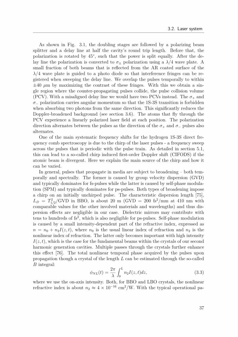
3.2. Laser system
As shown in Fig. 3.1, the doubling stages are followed by a polarizing beamsplitter and a delay line at half the cavity’s round trip length. Before that, thepolarization is rotated by 45, such that the power is split equally. After the de-lay line the polarization is converted to σ± polarization using a λ/4 wave plate. Asmall fraction of both beams that is reflected from the AR coated surface of theλ/4 wave plate is guided to a photo diode so that interference fringes can be re-gistered when sweeping the delay line. We overlap the pulses temporally to within±40 µm by maximizing the contrast of these fringes. With this we obtain a sin-gle region where the counter-propagating pulses collide, the pulse collision volume(PCV). With a misaligned delay line we would have two PCVs instead. The σ+ andσ− polarization carries angular momentum so that the 1S-3S transition is forbiddenwhen absorbing two photons from the same direction. This significantly reduces theDoppler-broadened background (see section 3.6). The atoms that fly through thePCV experience a linearly polarized laser field at each position. The polarizationdirection alternates between the pulses as the direction of the σ+ and σ− pulses alsoalternates.
One of the main systematic frequency shifts for the hydrogen 1S-3S direct fre-quency comb spectroscopy is due to the chirp of the laser pulses - a frequency sweepacross the pulses that is periodic with the pulse train. As detailed in section 5.1,this can lead to a so-called chirp induced first-order Doppler shift (CIFODS) if theatomic beam is divergent. Here we explain the main source of the chirp and how itcan be varied.
In general, pulses that propagate in media are subject to broadening – both tem-porally and spectrally. The former is caused by group velocity dispersion (GVD)and typically dominates for fs-pulses while the latter is caused by self-phase modula-tion (SPM) and typically dominates for ps-pulses. Both types of broadening imposea chirp on an initially unchirped pulse. The characteristic dispersion length [75],LD = T 2
1/2/GVD in BBO, is about 20 m (GVD = 200 fs2/mm at 410 nm withcomparable values for the other involved materials and wavelengths) and thus dis-persion effects are negligible in our case. Dielectric mirrors may contribute withtens to hundreds of fs2, which is also negligible for ps-pulses. Self-phase modulationis caused by a small intensity-dependent part of the refractive index, expressed asn = n0 + n2I(z, t), where n0 is the usual linear index of refraction and n2 is thenonlinear index of refraction. The latter only becomes important with high intensityI(z, t), which is the case for the fundamental beams within the crystals of our secondharmonic generation cavities. Multiple passes through the crystals further enhancethis effect [76]. The total nonlinear temporal phase acquired by the pulses uponpropagation though a crystal of the length L can be estimated through the so-calledB integral:
φNL(t) = 2πλ
∫ L
0n2I(z, t)dz, (3.3)
where we use the on-axis intensity. Both, for BBO and LBO crystals, the nonlinearrefractive index is about n2 ≈ 4 × 10⁻¹⁶ cm2/W. With the typical operational pa-
37
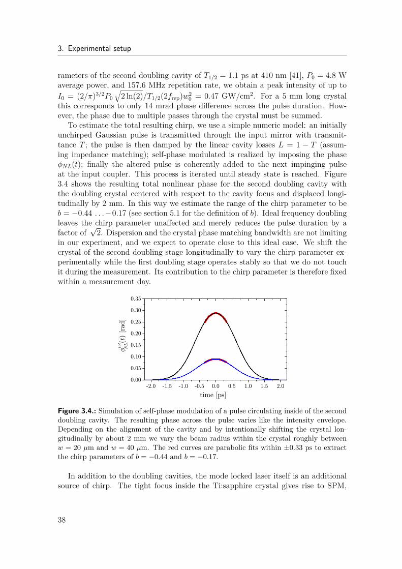
3. Experimental setup
rameters of the second doubling cavity of T1/2 = 1.1 ps at 410 nm [41], P0 = 4.8 Waverage power, and 157.6 MHz repetition rate, we obtain a peak intensity of up toI0 = (2/π)3/2P0
√2 ln(2)/T1/2(2frep)w2
0 = 0.47 GW/cm2. For a 5 mm long crystalthis corresponds to only 14 mrad phase difference across the pulse duration. How-ever, the phase due to multiple passes through the crystal must be summed.
To estimate the total resulting chirp, we use a simple numeric model: an initiallyunchirped Gaussian pulse is transmitted through the input mirror with transmit-tance T ; the pulse is then damped by the linear cavity losses L = 1 − T (assum-ing impedance matching); self-phase modulated is realized by imposing the phaseφNL(t); finally the altered pulse is coherently added to the next impinging pulseat the input coupler. This process is iterated until steady state is reached. Figure3.4 shows the resulting total nonlinear phase for the second doubling cavity withthe doubling crystal centered with respect to the cavity focus and displaced longi-tudinally by 2 mm. In this way we estimate the range of the chirp parameter to beb = −0.44 . . .−0.17 (see section 5.1 for the definition of b). Ideal frequency doublingleaves the chirp parameter unaffected and merely reduces the pulse duration by afactor of
√2. Dispersion and the crystal phase matching bandwidth are not limiting
in our experiment, and we expect to operate close to this ideal case. We shift thecrystal of the second doubling stage longitudinally to vary the chirp parameter ex-perimentally while the first doubling stage operates stably so that we do not touchit during the measurement. Its contribution to the chirp parameter is therefore fixedwithin a measurement day.
Figure 3.4.: Simulation of self-phase modulation of a pulse circulating inside of the seconddoubling cavity. The resulting phase across the pulse varies like the intensity envelope.Depending on the alignment of the cavity and by intentionally shifting the crystal lon-gitudinally by about 2 mm we vary the beam radius within the crystal roughly betweenw = 20 µm and w = 40 µm. The red curves are parabolic fits within ±0.33 ps to extractthe chirp parameters of b = −0.44 and b = −0.17.
In addition to the doubling cavities, the mode locked laser itself is an additionalsource of chirp. The tight focus inside the Ti:sapphire crystal gives rise to SPM,
38
3.2. Laser system
which in this laser (Spectra Physics, Tsunami) is compensated with an intra-cavityGires-Tournois interferometer. The length of this interferometer is controlled via apiezo transducer. Adjusting its voltage also varies the chirp parameter. However,this contribution to the chirp depends on other alignment parameters of the laserand is difficult to quantify. Like the first doubling stage, the laser operates stablyand is not often realigned. To first-order, the chirp parameters from the differentsources add. Experimentally we observe chirp parameter variations of ∆b = 0.38(see see Fig. 5.5), which is somewhat larger than that obtained by modeling thecontribution of only one doubling cavity. We believe this is because the contributionsfrom both doubling cavities add to the initial chirp from the laser. Moreover, theexperimental parameters may not be exactly the ones used in the model and varywith the alignment of the setup. For the data analysis we do not rely on knowledgeof the chirp parameter. It is sufficient to be able to modify it (see section 5.1).
It should be noted that it is not an easy task to measure a chirp described abovefor ps-pulses, since most phase/amplitude determining devices (such as FROG, SPI-DER) rely on the measurement of the (narrow) spectral width. Chirps due to SPMlead to a spectral broadening by a factor of about
√1 + b2 (i.e. by roughly 1% to
10% in our case), which is in the range of the observational broadening due to thefinite spectral resolution of the spectrometer.
39
3. Experimental setup
3.3. Mode suppressionThe doubling cavities, as described in the previous section, are designed to not onlydouble the optical carrier frequency, but also the repetition rate of the laser. Thisprocess is not perfect, and we are left with residual “unwanted” modes from the laserthat are not resonantly coupled into the doubling cavities. In an empty cavity, thesuppression of the unwanted modes is quite effective because the resonant modes areenhanced while the non-resonant modes are attenuated – even with a low finesse.With several cavities in series one expects a rather good suppression. However, thenonlinear crystals remix the modes and compromise the suppression ratio from whatis naively expected.
To estimate the strength of the unwanted modes, we use a simple model andassume a frequency comb of N modes that operates with a repetition rate of ωr =2πfrep and has a flat spectral envelope. The field coupled to the first doubling cavityis proportional to:
E(t) ∝∑n
Eneinωrt with En =
√T for n odd
1/√T for n even (3.4)
Here we assume that the impedance-matched even modes are resonant so that theirfields are enhanced by 1/
√T with the input coupler power transmission T given in
the previous section. The fields of the off-resonant odd modes are suppressed bythe inverse factor. The second harmonic field is proportional to the square of thefundamental field, i.e.:
E2(t) ∝∑n,n′
EnEn′ei(n+n′)ωrt with EnEn′ =
1 for n+ n′ odd1/T for n and n′ evenT ≈ 0 for n and n′ odd
(3.5)
Neglecting the terms that correspond to the last case, we find:
E2(t) ∝ 1T
∑n, n′
(n+ n′ even)
ei(n+n′)ωrt +∑n, n′
(n+ n′ odd)
ei(n+n′)ωrt = 1T
N
2∑n
ei2nωrt + N
2∑n
ei(2n+1)ωrt (3.6)
The first term represents the frequency doubled resonant modes and the second termare the unwanted off-resonant modes. It is seen that the power of the unwantedmodes are suppressed by a factor T 2 after the first doubling stage. Note that usingthe suppression ratio of the fundamental light and squaring it to take the secondharmonic generation into account yields the wrong result.
The action of the second doubling stage can be treated in a similar way. It is de-signed with the same input coupler transmission of T = 30%. Again, we assume thatthe even modes are enhanced by 1/
√T while the odd modes are further suppressed
40
3.3. Mode suppression
by√T :
E4(t) ∝(
1T 3/2
∑n
ei2nωrt +√T∑n
ei(2n+1)ωrt)2
= 1T 3
∑n,n′
ei2(n+n′)ωrt + T∑n,n′
ei(2(n+n′)+2)ωrt
︸ ︷︷ ︸≈0
+ 2T
∑n,n′
ei(2(n+n′)+1)ωrt. (3.7)
The first two terms are obviously the desired even modes while the last one representsthe unwanted odd modes at the fourth harmonic of the laser. We may neglect theterms proportional to T relative to the terms proportional to 1/T . As a result,the power of the unwanted modes of the frequency comb at 205 nm are suppressedby T 4 = 0.0081 relative to the desired modes with twice the mode spacing of thelaser-generated comb at 820 nm. This estimated suppression ratio is important todetermine the associated systematic shifts that are discussed in section 5.9.
41
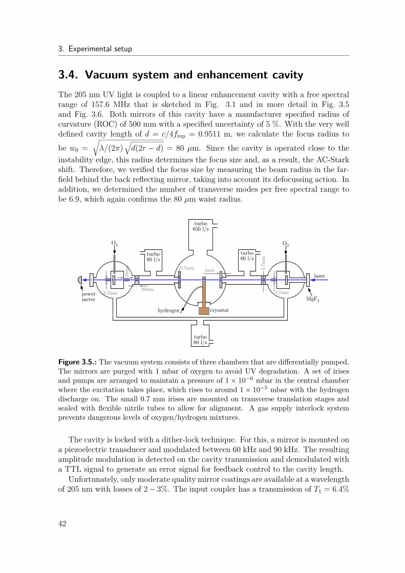
3. Experimental setup
3.4. Vacuum system and enhancement cavityThe 205 nm UV light is coupled to a linear enhancement cavity with a free spectralrange of 157.6 MHz that is sketched in Fig. 3.1 and in more detail in Fig. 3.5and Fig. 3.6. Both mirrors of this cavity have a manufacturer specified radius ofcurvature (ROC) of 500 mm with a specified uncertainty of 5 %. With the very welldefined cavity length of d = c/4frep = 0.9511 m, we calculate the focus radius tobe w0 =
√λ/(2π)
√d(2r − d) = 80 µm. Since the cavity is operated close to the
instability edge, this radius determines the focus size and, as a result, the AC-Starkshift. Therefore, we verified the focus size by measuring the beam radius in the far-field behind the back reflecting mirror, taking into account its defocussing action. Inaddition, we determined the number of transverse modes per free spectral range tobe 6.9, which again confirms the 80 µm waist radius.
turbo650 l/s
turbo80 l/s
turbo80 l/s
turbo80 l/s
O2O2
cryostat
laser
powermeter
20mm
3.7m
m
3.7mm
0.7mm 4mm
3.7mm
10m
m
MgF2
hydrogen
Figure 3.5.: The vacuum system consists of three chambers that are differentially pumped.The mirrors are purged with 1 mbar of oxygen to avoid UV degradation. A set of irisesand pumps are arranged to maintain a pressure of 1 × 10⁻⁶ mbar in the central chamberwhere the excitation takes place, which rises to around 1× 10⁻⁵ mbar with the hydrogendischarge on. The small 0.7 mm irises are mounted on transverse translation stages andsealed with flexible nitrile tubes to allow for alignment. A gas supply interlock systemprevents dangerous levels of oxygen/hydrogen mixtures.
The cavity is locked with a dither-lock technique. For this, a mirror is mounted ona piezoelectric transducer and modulated between 60 kHz and 90 kHz. The resultingamplitude modulation is detected on the cavity transmission and demodulated witha TTL signal to generate an error signal for feedback control to the cavity length.
Unfortunately, only moderate quality mirror coatings are available at a wavelengthof 205 nm with losses of 2− 3%. The input coupler has a transmission of T1 = 6.4%
42
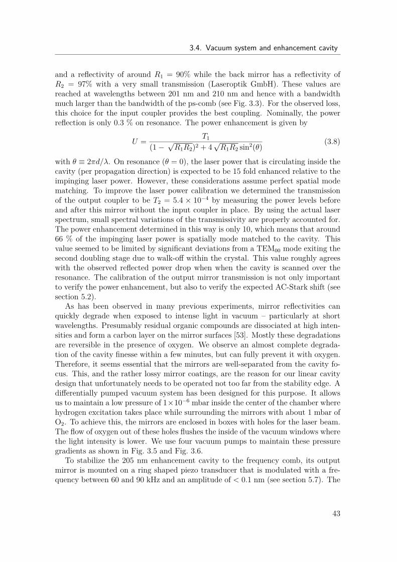
3.4. Vacuum system and enhancement cavity
and a reflectivity of around R1 = 90% while the back mirror has a reflectivity ofR2 = 97% with a very small transmission (Laseroptik GmbH). These values arereached at wavelengths between 201 nm and 210 nm and hence with a bandwidthmuch larger than the bandwidth of the ps-comb (see Fig. 3.3). For the observed loss,this choice for the input coupler provides the best coupling. Nominally, the powerreflection is only 0.3 % on resonance. The power enhancement is given by
U = T1
(1−√R1R2)2 + 4
√R1R2 sin2(θ)
(3.8)
with θ ≡ 2πd/λ. On resonance (θ = 0), the laser power that is circulating inside thecavity (per propagation direction) is expected to be 15 fold enhanced relative to theimpinging laser power. However, these considerations assume perfect spatial modematching. To improve the laser power calibration we determined the transmissionof the output coupler to be T2 = 5.4 × 10⁻⁴ by measuring the power levels beforeand after this mirror without the input coupler in place. By using the actual laserspectrum, small spectral variations of the transmissivity are properly accounted for.The power enhancement determined in this way is only 10, which means that around66 % of the impinging laser power is spatially mode matched to the cavity. Thisvalue seemed to be limited by significant deviations from a TEM00 mode exiting thesecond doubling stage due to walk-off within the crystal. This value roughly agreeswith the observed reflected power drop when when the cavity is scanned over theresonance. The calibration of the output mirror transmission is not only importantto verify the power enhancement, but also to verify the expected AC-Stark shift (seesection 5.2).
As has been observed in many previous experiments, mirror reflectivities canquickly degrade when exposed to intense light in vacuum – particularly at shortwavelengths. Presumably residual organic compounds are dissociated at high inten-sities and form a carbon layer on the mirror surfaces [53]. Mostly these degradationsare reversible in the presence of oxygen. We observe an almost complete degrada-tion of the cavity finesse within a few minutes, but can fully prevent it with oxygen.Therefore, it seems essential that the mirrors are well-separated from the cavity fo-cus. This, and the rather lossy mirror coatings, are the reason for our linear cavitydesign that unfortunately needs to be operated not too far from the stability edge. Adifferentially pumped vacuum system has been designed for this purpose. It allowsus to maintain a low pressure of 1×10⁻⁶ mbar inside the center of the chamber wherehydrogen excitation takes place while surrounding the mirrors with about 1 mbar ofO2. To achieve this, the mirrors are enclosed in boxes with holes for the laser beam.The flow of oxygen out of these holes flushes the inside of the vacuum windows wherethe light intensity is lower. We use four vacuum pumps to maintain these pressuregradients as shown in Fig. 3.5 and Fig. 3.6.
To stabilize the 205 nm enhancement cavity to the frequency comb, its outputmirror is mounted on a ring shaped piezo transducer that is modulated with a fre-quency between 60 and 90 kHz and an amplitude of < 0.1 nm (see section 5.7). The
43
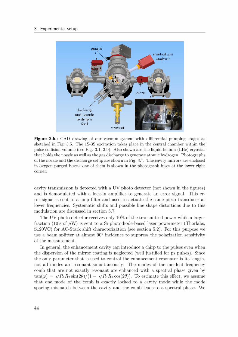
3. Experimental setup
Figure 3.6.: CAD drawing of our vacuum system with differential pumping stages assketched in Fig. 3.5. The 1S-3S excitation takes place in the central chamber within thepulse collision volume (see Fig. 3.1, 3.9). Also shown are the liquid helium (LHe) cryostatthat holds the nozzle as well as the gas discharge to generate atomic hydrogen. Photographsof the nozzle and the discharge setup are shown in Fig. 3.7. The cavity mirrors are enclosedin oxygen purged boxes; one of them is shown in the photograph inset at the lower rightcorner.
cavity transmission is detected with a UV photo detector (not shown in the figures)and is demodulated with a lock-in amplifier to generate an error signal. This er-ror signal is sent to a loop filter and used to actuate the same piezo transducer atlower frequencies. Systematic shifts and possible line shape distortions due to thismodulation are discussed in section 5.7.
The UV photo detector receives only 10% of the transmitted power while a largerfraction (10’s of µW) is sent to a Si photodiode-based laser powermeter (Thorlabs,S120VC) for AC-Stark shift characterization (see section 5.2). For this purpose weuse a beam splitter at almost 90 incidence to suppress the polarization sensitivityof the measurement.
In general, the enhancement cavity can introduce a chirp to the pulses even whenthe dispersion of the mirror coating is neglected (well justified for ps pulses). Sincethe only parameter that is used to control the enhancement resonator is its length,not all modes are resonant simultaneously. The modes of the incident frequencycomb that are not exactly resonant are enhanced with a spectral phase given bytan(ϕ) =
√R1R2 sin(2θ)/(1 −
√R1R2 cos(2θ)). To estimate this effect, we assume
that one mode of the comb is exactly locked to a cavity mode while the modespacing mismatch between the cavity and the comb leads to a spectral phase. We
44
3.4. Vacuum system and enhancement cavity
further assume that the free running carrier envelope offset frequency of the combis less than the repetition rate. The maximum offset within its spectral width of∆ω = 2π × 148 GHz is reduced by the relative optical bandwidth of 1.0 × 10⁻⁴,i.e. θmax = 1.0 × 10⁻⁴π and |ϕ| = 8.9 mrad. While a linear spectral phase doesnot chirp the pulses, we assume that the cavity imposed spectral phase is purelyquadratic. This leads to a pulse broadening of
√1 + (2θmax/τ 2∆ω)2 = 1.000013 and
a corresponding chirp parameter of b = 0.0051 that can be safely ignored.
45
3. Experimental setup
3.5. Atomic hydrogen beamTo form a cryogenic atomic hydrogen beam [54], we first dissociate molecular hydro-gen in a gas discharge. A 6 mm diameter Pyrex tube is surrounded by a 2.4 GHz radiofrequency cavity with 30 W of input power. The pressure inside the tube is around8.6 mbar and the total hydrogen flux is very constant at around 0.37 ml/min (1.7×10¹⁷ molecules/s) and continually monitored with a mass flow meter (Bronkhorst,EL-Flow). At the outlet of the tube there is a small orifice (300 − 500 µm diame-ter). Behind the orifice a 30 cm long Teflon tube with 4 mm inner diameter (6 mmouter diameter) guides the dissociated hydrogen into the copper nozzle. The noz-zle consists of a box-shaped reservoir (inner dimensions 7.8 × 7.0 × 9.4 mm3) withtwo orifices through which hydrogen escapes into vacuum and which allow the laserbeam to pass through the nozzle. The orifice that faces the pulse collision volume(PCV) has a diameter of 1.5 mm and the rear orifice a diameter of 1.3 mm. Weuse a liquid helium flow cryostat (ICE Oxford) to cool the nozzle (minimal tempe-rature 4 K). A short part of the Teflon tube (∼ 8 mm) is clamped to the nozzlefor mounting and is assumed to be at a temperature close to that of the nozzle.The temperature is measured both inside the copper cooling head of the cryostat(sensor: LakeShore, CX-1030-AA-1.4L) and on top of the hydrogen nozzle abovethe thermalization volume (sensor: Lake Shore DT-670B-SD). The temperature isstabilized to within 10 mK through a feedback loop (heating wire inside the cool-ing head). Good temperature stability is not only important for characterizing thesecond-order Doppler effect (see section 5.3), but also to reduce excess noise becausethe flow of atomic hydrogen critically depends on the nozzle temperature. Figure 3.7shows photographs of the discharge tube and the nozzle.
The hydrogen atoms thermalize to the nozzle’s temperature through collisionswith the cold walls of the nozzle’s reservoir and the cold section of the Teflon tube,or collisions with other atoms or molecules, with at least one collision necessaryfor the atoms to leave the nozzle. Using a particle tracing simulation, the numberof collisions the atoms undergo with these cold walls before leaving the nozzle isestimated. Collisions between the particles are not included in the simulation, butare thought to increase the total number of collisions above the number of wallcollisions. The mean number of wall collisions is found to be 60, with most of theatoms undergoing 15 collisions. In total, 99.6% of the atoms undergo more thanone wall collision. We expect this number of collisions to be sufficient for goodthermalization based on the observations of [54, 62] where nozzle designs with asimilar number of collisions were studied. We note that, due to the nozzle’s geometry,atoms traveling on-axis with the laser beam can only originate from collisions withother atoms or molecules and not from the cold walls. In fact, collisions betweenthese particles should allow for faster thermalization than wall collisions, since themass ratios of the collision partners are well matched. However, these collisions alsotend to remove slower atoms from the beam, as discussed in section 5.3.
In first order a thermal beam of atoms may be described with a Maxwellian
46
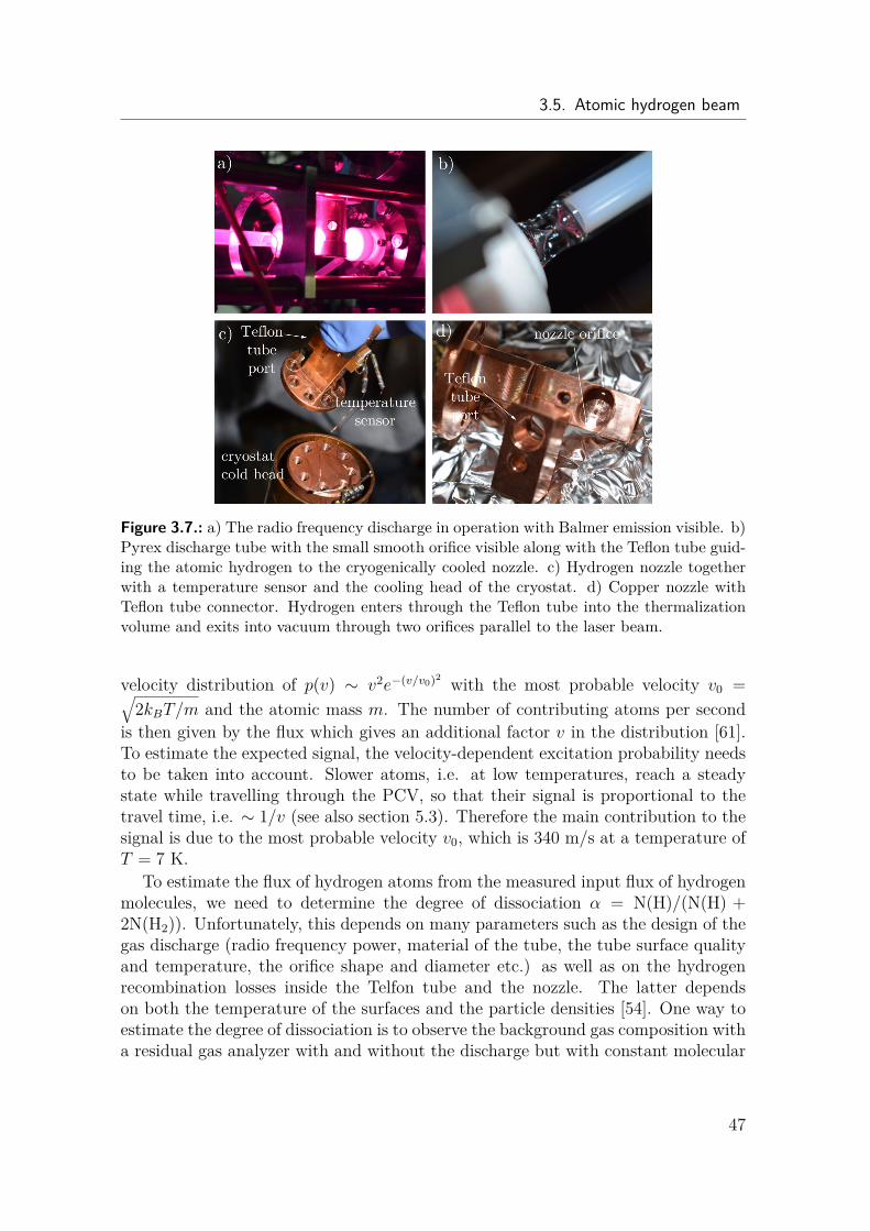
3.5. Atomic hydrogen beam
Figure 3.7.: a) The radio frequency discharge in operation with Balmer emission visible. b)Pyrex discharge tube with the small smooth orifice visible along with the Teflon tube guid-ing the atomic hydrogen to the cryogenically cooled nozzle. c) Hydrogen nozzle togetherwith a temperature sensor and the cooling head of the cryostat. d) Copper nozzle withTeflon tube connector. Hydrogen enters through the Teflon tube into the thermalizationvolume and exits into vacuum through two orifices parallel to the laser beam.
velocity distribution of p(v) ∼ v2e−(v/v0)2 with the most probable velocity v0 =√2kBT/m and the atomic mass m. The number of contributing atoms per second
is then given by the flux which gives an additional factor v in the distribution [61].To estimate the expected signal, the velocity-dependent excitation probability needsto be taken into account. Slower atoms, i.e. at low temperatures, reach a steadystate while travelling through the PCV, so that their signal is proportional to thetravel time, i.e. ∼ 1/v (see also section 5.3). Therefore the main contribution to thesignal is due to the most probable velocity v0, which is 340 m/s at a temperature ofT = 7 K.
To estimate the flux of hydrogen atoms from the measured input flux of hydrogenmolecules, we need to determine the degree of dissociation α = N(H)/(N(H) +2N(H2)). Unfortunately, this depends on many parameters such as the design of thegas discharge (radio frequency power, material of the tube, the tube surface qualityand temperature, the orifice shape and diameter etc.) as well as on the hydrogenrecombination losses inside the Telfon tube and the nozzle. The latter dependson both the temperature of the surfaces and the particle densities [54]. One way toestimate the degree of dissociation is to observe the background gas composition witha residual gas analyzer with and without the discharge but with constant molecular
47
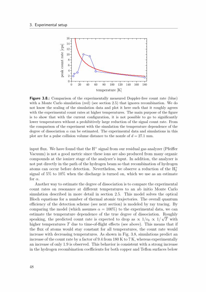
3. Experimental setup
0 2 0 4 0 6 0 8 0 1 0 0 1 2 0 1 4 0 1 6 0 1 8 002468
1 01 21 41 6
peak c
ount
rate [
cps]
t e m p e r a t u r e [ K ]Figure 3.8.: Comparison of the experimentally measured Doppler-free count rate (blue)with a Monte Carlo simulation (red) (see section 2.5) that ignores recombination. We donot know the scaling of the simulation data and plot it here such that it roughly agreeswith the experimental count rates at higher temperatures. The main purpose of the figureis to show that with the current configuration, it is not possible to go to significantlylower temperatures without a prohibitively large reduction of the signal count rate. Fromthe comparison of the experiment with the simulation the temperature dependence of thedegree of dissociation α can be estimated. The experimental data and simulations in thisplot are for a pulse collision volume distance to the nozzle of d = 27.1 mm.
input flux. We have found that the H+ signal from our residual gas analyzer (PfeifferVacuum) is not a good metric since these ions are also produced from many organiccompounds at the ionizer stage of the analyzer’s input. In addition, the analyzer isnot put directly in the path of the hydrogen beam so that recombination of hydrogenatoms can occur before detection. Nevertheless, we observe a reduction of the H+
2signal of 5% to 10% when the discharge is turned on, which we use as an estimatefor α.
Another way to estimate the degree of dissociation is to compare the experimentalcount rates on resonance at different temperatures to an ab initio Monte Carlosimulation described in more detail in section 2.5. This model solves the opticalBloch equations for a number of thermal atomic trajectories. The overall quantumefficiency of the detection scheme (see next section) is modeled by ray tracing. Bycomparing the model (which assumes α = 100%) to the experimental data, we canestimate the temperature dependence of the true degree of dissociation. Roughlyspeaking, the predicted count rate is expected to drop as ∝ 1/v0 ∝ 1/
√T with
higher temperatures T due to time-of-flight effects (see above). This means that ifthe flux of atoms would stay constant for all temperatures, the count rate wouldincrease with decreasing temperatures. As shown in Fig. 3.8, simulations predict anincrease of the count rate by a factor of 9.4 from 180 K to 7 K, whereas experimentallyan increase of only 1.9 is observed. This behavior is consistent with a strong increasein the hydrogen recombination coefficients for both copper and Teflon surfaces below
48
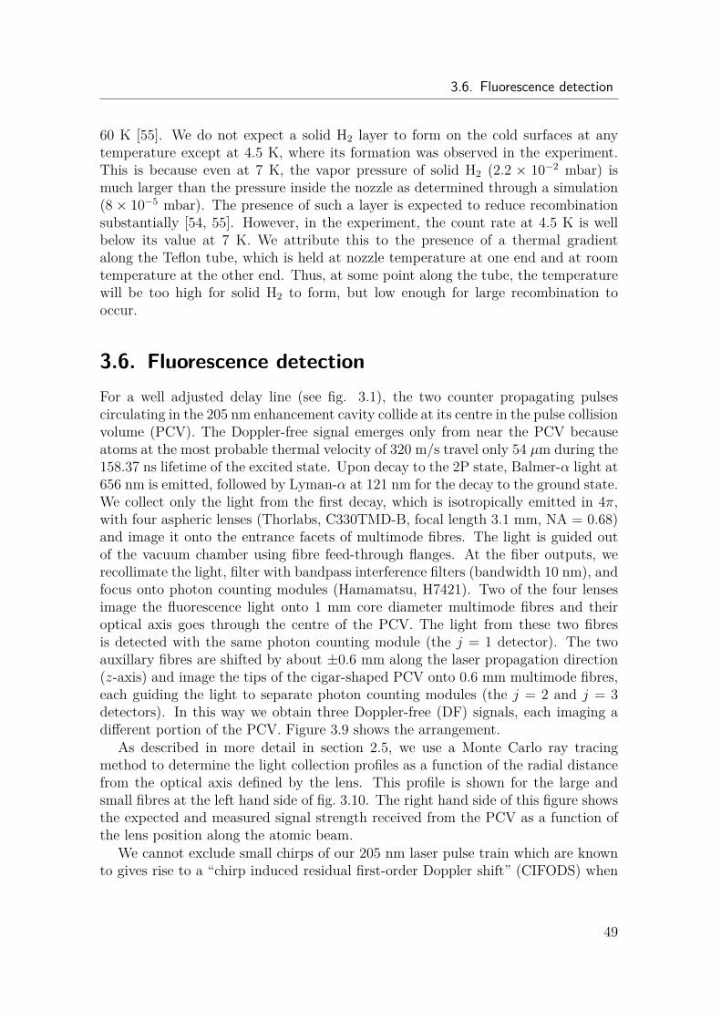
3.6. Fluorescence detection
60 K [55]. We do not expect a solid H2 layer to form on the cold surfaces at anytemperature except at 4.5 K, where its formation was observed in the experiment.This is because even at 7 K, the vapor pressure of solid H2 (2.2 × 10⁻² mbar) ismuch larger than the pressure inside the nozzle as determined through a simulation(8× 10⁻⁵ mbar). The presence of such a layer is expected to reduce recombinationsubstantially [54, 55]. However, in the experiment, the count rate at 4.5 K is wellbelow its value at 7 K. We attribute this to the presence of a thermal gradientalong the Teflon tube, which is held at nozzle temperature at one end and at roomtemperature at the other end. Thus, at some point along the tube, the temperaturewill be too high for solid H2 to form, but low enough for large recombination tooccur.
3.6. Fluorescence detectionFor a well adjusted delay line (see fig. 3.1), the two counter propagating pulsescirculating in the 205 nm enhancement cavity collide at its centre in the pulse collisionvolume (PCV). The Doppler-free signal emerges only from near the PCV becauseatoms at the most probable thermal velocity of 320 m/s travel only 54 µm during the158.37 ns lifetime of the excited state. Upon decay to the 2P state, Balmer-α light at656 nm is emitted, followed by Lyman-α at 121 nm for the decay to the ground state.We collect only the light from the first decay, which is isotropically emitted in 4π,with four aspheric lenses (Thorlabs, C330TMD-B, focal length 3.1 mm, NA = 0.68)and image it onto the entrance facets of multimode fibres. The light is guided outof the vacuum chamber using fibre feed-through flanges. At the fiber outputs, werecollimate the light, filter with bandpass interference filters (bandwidth 10 nm), andfocus onto photon counting modules (Hamamatsu, H7421). Two of the four lensesimage the fluorescence light onto 1 mm core diameter multimode fibres and theiroptical axis goes through the centre of the PCV. The light from these two fibresis detected with the same photon counting module (the j = 1 detector). The twoauxillary fibres are shifted by about ±0.6 mm along the laser propagation direction(z-axis) and image the tips of the cigar-shaped PCV onto 0.6 mm multimode fibres,each guiding the light to separate photon counting modules (the j = 2 and j = 3detectors). In this way we obtain three Doppler-free (DF) signals, each imaging adifferent portion of the PCV. Figure 3.9 shows the arrangement.
As described in more detail in section 2.5, we use a Monte Carlo ray tracingmethod to determine the light collection profiles as a function of the radial distancefrom the optical axis defined by the lens. This profile is shown for the large andsmall fibres at the left hand side of fig. 3.10. The right hand side of this figure showsthe expected and measured signal strength received from the PCV as a function ofthe lens position along the atomic beam.
We cannot exclude small chirps of our 205 nm laser pulse train which are knownto gives rise to a “chirp induced residual first-order Doppler shift” (CIFODS) when
49
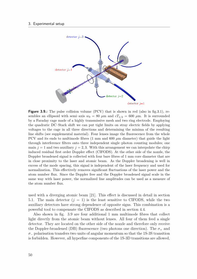
3. Experimental setup
Figure 3.9.: The pulse collision volume (PCV) that is shown in red (also in fig.3.1), re-sembles an ellipsoid with semi–axis w0 = 80 µm and cT1/2 = 600 µm. It is surroundedby a Faraday cage made of a highly transmissive mesh and two ring electrode. Employingthe quadratic DC–Stark shift we can put tight limits on stray electric fields by applyingvoltages to the cage in all three directions and determining the minima of the resultingline shifts (see supplemental material). Four lenses image the fluorescence from the wholePCV and its ends to multimode fibres (1 mm and 600 µm diameter) that guide the lightthrough interference filters onto three independent single–photon counting modules; onemain j = 1 and two auxiliary j = 2, 3. With this arrangement we can interpolate the chirpinduced residual first order Doppler effect (CIFODS). At the other side of the nozzle, theDoppler broadened signal is collected with four bare fibres of 1 mm core diameter that arein close proximity to the laser and atomic beam. As the Doppler broadening is well inexcess of the mode spacing, this signal is independent of the laser frequency and used fornormalization. This effectively removes significant fluctuations of the laser power and theatom number flux. Since the Doppler free and the Doppler broadened signal scale in thesame way with laser power, the normalized line amplitudes can be used as a measure ofthe atom number flux.
used with a diverging atomic beam [21]. This effect is discussed in detail in section5.1. The main detector (j = 1) is the least sensitive to CIFODS, while the twoauxiliary detectors have strong dependence of opposite signs. This combination is apowerful tool to compensate the CIFODS as described in section 4.4.
Also shown in fig. 3.9 are four additional 1 mm multimode fibres that collectlight directly from the atomic beam without lenses. All four of them feed a singledetector. They are located on the other side of the nozzle and therefore only receivethe Doppler-broadened (DB) fluorescence (two photons one direction). The σ+ andσ− polarisation transfers two units of angular momentum so that the 1S-3S transitionis forbidden. However, all hyperfine components of the 1S-3D transitions are allowed,
50
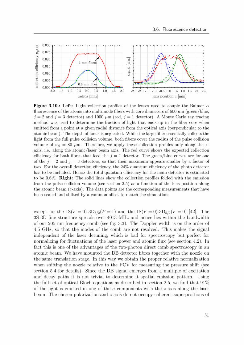
3.6. Fluorescence detection
Figure 3.10.: Left: Light collection profiles of the lenses used to couple the Balmer–αfluorescence of the atoms into multimode fibers with core diameters of 600 µm (green/blue,j = 2 and j = 3 detector) and 1000 µm (red, j = 1 detector). A Monte Carlo ray tracingmethod was used to determine the fraction of light that ends up in the fiber core whenemitted from a point at a given radial distance from the optical axis (perpendicular to theatomic beam). The depth of focus is neglected. While the large fiber essentially collects thelight from the full pulse collision volume, both fibers cover the radius of the pulse collisionvolume of w0 = 80 µm. Therefore, we apply these collection profiles only along the z-axis, i.e. along the atomic/laser beam axis. The red curve shows the expected collectionefficiency for both fibres that feed the j = 1 detector. The green/blue curves are for oneof the j = 2 and j = 3 detectors, so that their maximum appears smaller by a factor oftwo. For the overall detection efficiency, the 24% quantum efficiency of the photo detectorhas to be included. Hence the total quantum efficiency for the main detector is estimatedto be 0.6%. Right: The solid lines show the collection profiles folded with the emissionfrom the pulse collision volume (see section 2.5) as a function of the lens position alongthe atomic beam (z-axis). The data points are the corresponding measurements that havebeen scaled and shifted by a common offset to match the simulations.
except for the 1S(F = 0)-3D3/2(F = 1) and the 1S(F = 0)-3D5/2(F = 0) [42]. The3S-3D fine structure spreads over 4013 MHz and hence lies within the bandwidthof our 205 nm frequency comb (see fig. 3.3). The Doppler width is on the order of4.5 GHz, so that the modes of the comb are not resolved. This makes the signalindependent of the laser detuning, which is bad for spectroscopy but perfect fornormalizing for fluctuations of the laser power and atomic flux (see section 4.2). Infact this is one of the advantages of the two-photon direct comb spectroscopy in anatomic beam. We have mounted the DB detector fibres together with the nozzle onthe same translation stage. In this way we obtain the proper relative normalizationwhen shifting the nozzle relative to the PCV for measuring the pressure shift (seesection 5.4 for details). Since the DB signal emerges from a multiple of excitationand decay paths it is not trivial to determine it spatial emission pattern. Usingthe full set of optical Bloch equations as described in section 2.5, we find that 91%of the light is emitted in one of the σ-components with the z-axis along the laserbeam. The chosen polarization and z-axis do not occupy coherent superpositions of
51
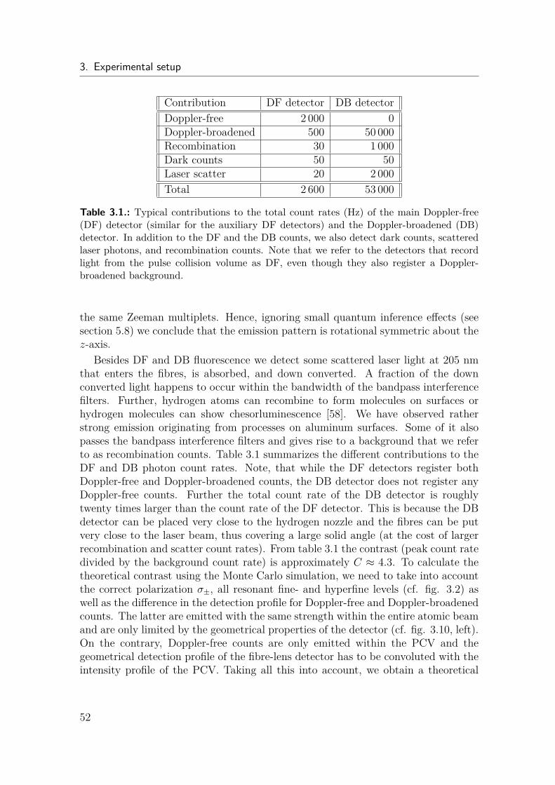
3. Experimental setup
Contribution DF detector DB detectorDoppler-free 2 000 0Doppler-broadened 500 50 000Recombination 30 1 000Dark counts 50 50Laser scatter 20 2 000Total 2 600 53 000
Table 3.1.: Typical contributions to the total count rates (Hz) of the main Doppler-free(DF) detector (similar for the auxiliary DF detectors) and the Doppler-broadened (DB)detector. In addition to the DF and the DB counts, we also detect dark counts, scatteredlaser photons, and recombination counts. Note that we refer to the detectors that recordlight from the pulse collision volume as DF, even though they also register a Doppler-broadened background.
the same Zeeman multiplets. Hence, ignoring small quantum inference effects (seesection 5.8) we conclude that the emission pattern is rotational symmetric about thez-axis.
Besides DF and DB fluorescence we detect some scattered laser light at 205 nmthat enters the fibres, is absorbed, and down converted. A fraction of the downconverted light happens to occur within the bandwidth of the bandpass interferencefilters. Further, hydrogen atoms can recombine to form molecules on surfaces orhydrogen molecules can show chesorluminescence [58]. We have observed ratherstrong emission originating from processes on aluminum surfaces. Some of it alsopasses the bandpass interference filters and gives rise to a background that we referto as recombination counts. Table 3.1 summarizes the different contributions to theDF and DB photon count rates. Note, that while the DF detectors register bothDoppler-free and Doppler-broadened counts, the DB detector does not register anyDoppler-free counts. Further the total count rate of the DB detector is roughlytwenty times larger than the count rate of the DF detector. This is because the DBdetector can be placed very close to the hydrogen nozzle and the fibres can be putvery close to the laser beam, thus covering a large solid angle (at the cost of largerrecombination and scatter count rates). From table 3.1 the contrast (peak count ratedivided by the background count rate) is approximately C ≈ 4.3. To calculate thetheoretical contrast using the Monte Carlo simulation, we need to take into accountthe correct polarization σ±, all resonant fine- and hyperfine levels (cf. fig. 3.2) aswell as the difference in the detection profile for Doppler-free and Doppler-broadenedcounts. The latter are emitted with the same strength within the entire atomic beamand are only limited by the geometrical properties of the detector (cf. fig. 3.10, left).On the contrary, Doppler-free counts are only emitted within the PCV and thegeometrical detection profile of the fibre-lens detector has to be convoluted with theintensity profile of the PCV. Taking all this into account, we obtain a theoretical
52
3.6. Fluorescence detection
contrast of approximately C ≈ 6.55, which is slightly better than the experimentallyobserved contrast.
53

4. Data Evaluation
4.1. Data DescriptionThe measurement campaign was carried out in two sessions in March and April of2018 with a total of 11 measurement days. The measurement data and descriptionfiles can be found in [50]. Different key parameters such as the nozzle temperature,its distance to the PCV, the laser power, and the chirp of the laser pulses werevaried in order to experimentally characterize systematics such as the second-orderDoppler shift, pressure shift, AC-Stark shift and residual first-order Doppler shifts(CIFODS). Overall 4450 valid line scans have been recorded, most of which contain21 data points of 1 s gate time with a total duration of 36 s (see Fig. 4.1). To improvethe statistics we do not distribute the data points uniformly on the frequency axisbut so that they appear roughly equidistant on the signal axis (see lower right ofFig. 4.2). For this we employed the following line sampling grid:
−4.000000 MHz −1.796820 MHz −1.271250 MHz −0.992032 MHz−0.804280 MHz −0.661160 MHz −0.542312 MHz −0.436248 MHz−0.334024 MHz −0.223112 MHz 0.000000 MHz
with the mirrored positive frequencies. In this way, we put additional weight on theparts of the line shape with the largest slope – that is with the largest sensitivity tothe line position. The frequency points are measured pairwise symmetric in randomorder but with the central point always first. Randomizing the sequence of mea-surement points is important. Otherwise the continuous degradation of the seconddoubling stage, as described in section 3.2, would lead to systematic line shifts.
Besides the cycle slip criteria described in section 3.1, we apply additional dataselection rules. To remove glitches in the laser power, for example by drop-outs ofthe 205 nm cavity lock, we discard points where the DB counts deviate by more than3 standard deviations from the line-averaged DB counts. We apply the same criteriato the recorded transmitted laser power through the cavity. In addition, we discardpoints that received less than 30% of the maximum DB counts of the respective linescan. We discard the full line scan if it contains less than 10 data points after theseselections. In total, we removed 5.6% of data points from the line scans and removeda total of 369 full line scans. Figure 4.1 gives an overview of the number of validdata points per line scan. We verified that the variation of the thresholds withinreasonable limits has no effect on our final result.
55
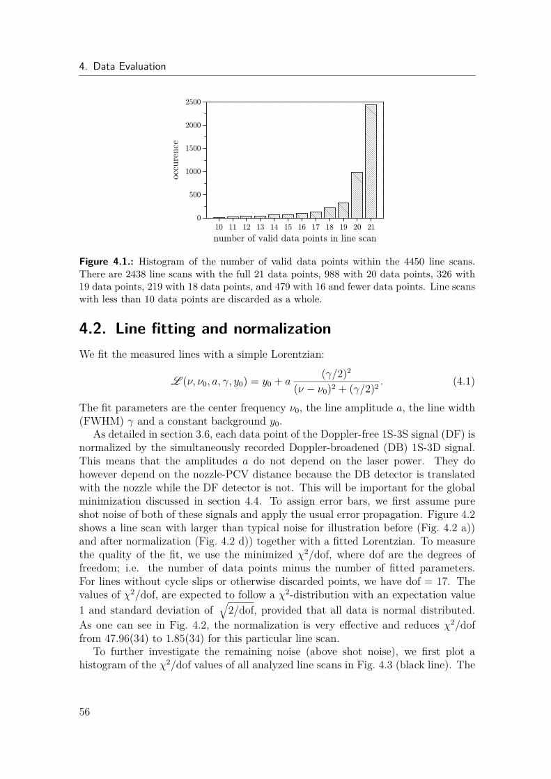
4. Data Evaluation
Figure 4.1.: Histogram of the number of valid data points within the 4450 line scans.There are 2438 line scans with the full 21 data points, 988 with 20 data points, 326 with19 data points, 219 with 18 data points, and 479 with 16 and fewer data points. Line scanswith less than 10 data points are discarded as a whole.
4.2. Line fitting and normalizationWe fit the measured lines with a simple Lorentzian:
L (ν, ν0, a, γ, y0) = y0 + a(γ/2)2
(ν − ν0)2 + (γ/2)2 . (4.1)
The fit parameters are the center frequency ν0, the line amplitude a, the line width(FWHM) γ and a constant background y0.
As detailed in section 3.6, each data point of the Doppler-free 1S-3S signal (DF) isnormalized by the simultaneously recorded Doppler-broadened (DB) 1S-3D signal.This means that the amplitudes a do not depend on the laser power. They dohowever depend on the nozzle-PCV distance because the DB detector is translatedwith the nozzle while the DF detector is not. This will be important for the globalminimization discussed in section 4.4. To assign error bars, we first assume pureshot noise of both of these signals and apply the usual error propagation. Figure 4.2shows a line scan with larger than typical noise for illustration before (Fig. 4.2 a))and after normalization (Fig. 4.2 d)) together with a fitted Lorentzian. To measurethe quality of the fit, we use the minimized χ2/dof, where dof are the degrees offreedom; i.e. the number of data points minus the number of fitted parameters.For lines without cycle slips or otherwise discarded points, we have dof = 17. Thevalues of χ2/dof, are expected to follow a χ2-distribution with an expectation value1 and standard deviation of
√2/dof, provided that all data is normal distributed.
As one can see in Fig. 4.2, the normalization is very effective and reduces χ2/doffrom 47.96(34) to 1.85(34) for this particular line scan.
To further investigate the remaining noise (above shot noise), we first plot ahistogram of the χ2/dof values of all analyzed line scans in Fig. 4.3 (black line). The
56
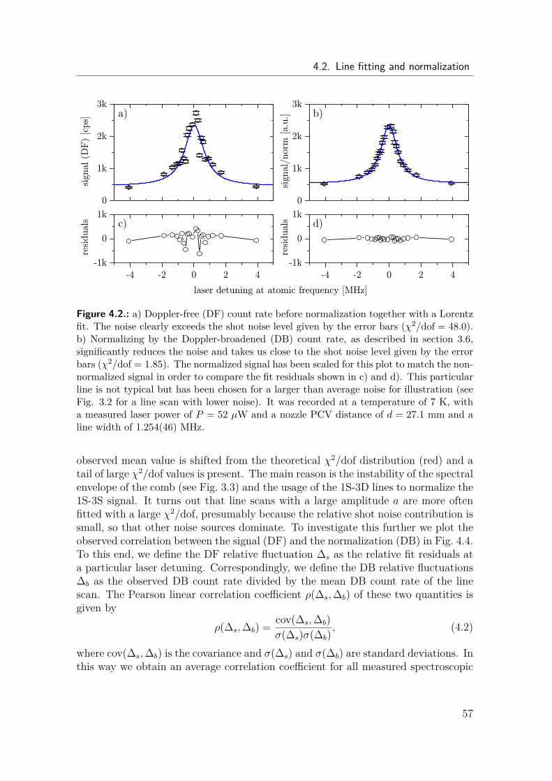
4.2. Line fitting and normalization
Figure 4.2.: a) Doppler-free (DF) count rate before normalization together with a Lorentzfit. The noise clearly exceeds the shot noise level given by the error bars (χ2/dof = 48.0).b) Normalizing by the Doppler-broadened (DB) count rate, as described in section 3.6,significantly reduces the noise and takes us close to the shot noise level given by the errorbars (χ2/dof = 1.85). The normalized signal has been scaled for this plot to match the non-normalized signal in order to compare the fit residuals shown in c) and d). This particularline is not typical but has been chosen for a larger than average noise for illustration (seeFig. 3.2 for a line scan with lower noise). It was recorded at a temperature of 7 K, witha measured laser power of P = 52 µW and a nozzle PCV distance of d = 27.1 mm and aline width of 1.254(46) MHz.
observed mean value is shifted from the theoretical χ2/dof distribution (red) and atail of large χ2/dof values is present. The main reason is the instability of the spectralenvelope of the comb (see Fig. 3.3) and the usage of the 1S-3D lines to normalize the1S-3S signal. It turns out that line scans with a large amplitude a are more oftenfitted with a large χ2/dof, presumably because the relative shot noise contribution issmall, so that other noise sources dominate. To investigate this further we plot theobserved correlation between the signal (DF) and the normalization (DB) in Fig. 4.4.To this end, we define the DF relative fluctuation ∆s as the relative fit residuals ata particular laser detuning. Correspondingly, we define the DB relative fluctuations∆b as the observed DB count rate divided by the mean DB count rate of the linescan. The Pearson linear correlation coefficient ρ(∆s,∆b) of these two quantities isgiven by
ρ(∆s,∆b) = cov(∆s,∆b)σ(∆s)σ(∆b)
, (4.2)
where cov(∆s,∆b) is the covariance and σ(∆s) and σ(∆b) are standard deviations. Inthis way we obtain an average correlation coefficient for all measured spectroscopic
57
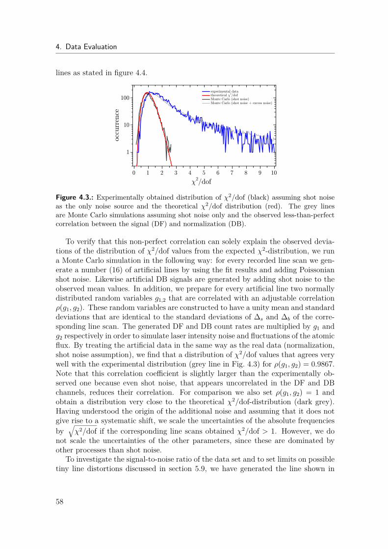
4. Data Evaluation
lines as stated in figure 4.4.
Figure 4.3.: Experimentally obtained distribution of χ2/dof (black) assuming shot noiseas the only noise source and the theoretical χ2/dof distribution (red). The grey linesare Monte Carlo simulations assuming shot noise only and the observed less-than-perfectcorrelation between the signal (DF) and normalization (DB).
To verify that this non-perfect correlation can solely explain the observed devia-tions of the distribution of χ2/dof values from the expected χ2-distribution, we runa Monte Carlo simulation in the following way: for every recorded line scan we gen-erate a number (16) of artificial lines by using the fit results and adding Poissonianshot noise. Likewise artificial DB signals are generated by adding shot noise to theobserved mean values. In addition, we prepare for every artificial line two normallydistributed random variables g1,2 that are correlated with an adjustable correlationρ(g1, g2). These random variables are constructed to have a unity mean and standarddeviations that are identical to the standard deviations of ∆s and ∆b of the corre-sponding line scan. The generated DF and DB count rates are multiplied by g1 andg2 respectively in order to simulate laser intensity noise and fluctuations of the atomicflux. By treating the artificial data in the same way as the real data (normalization,shot noise assumption), we find that a distribution of χ2/dof values that agrees verywell with the experimental distribution (grey line in Fig. 4.3) for ρ(g1, g2) = 0.9867.Note that this correlation coefficient is slightly larger than the experimentally ob-served one because even shot noise, that appears uncorrelated in the DF and DBchannels, reduces their correlation. For comparison we also set ρ(g1, g2) = 1 andobtain a distribution very close to the theoretical χ2/dof-distribution (dark grey).Having understood the origin of the additional noise and assuming that it does notgive rise to a systematic shift, we scale the uncertainties of the absolute frequenciesby
√χ2/dof if the corresponding line scans obtained χ2/dof > 1. However, we do
not scale the uncertainties of the other parameters, since these are dominated byother processes than shot noise.
To investigate the signal-to-noise ratio of the data set and to set limits on possibletiny line distortions discussed in section 5.9, we have generated the line shown in
58
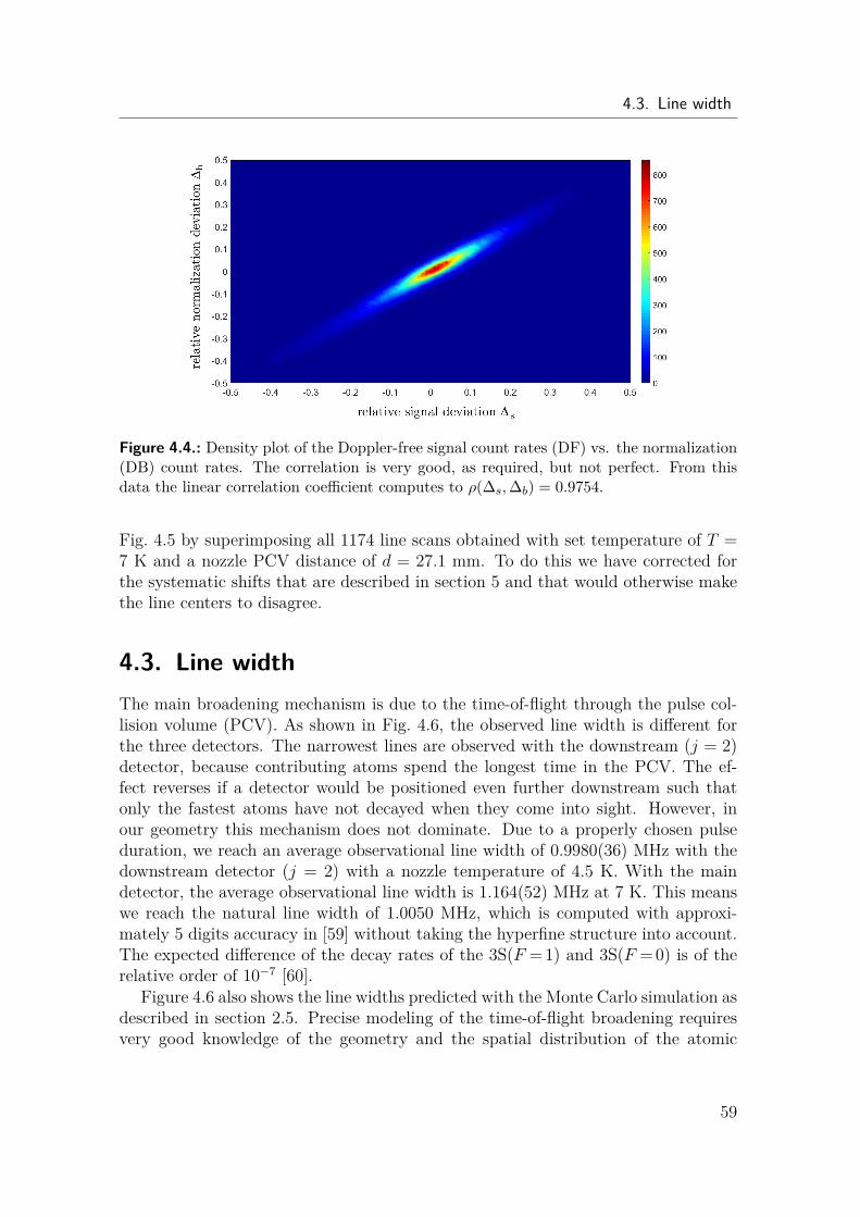
4.3. Line width
Figure 4.4.: Density plot of the Doppler-free signal count rates (DF) vs. the normalization(DB) count rates. The correlation is very good, as required, but not perfect. From thisdata the linear correlation coefficient computes to ρ(∆s,∆b) = 0.9754.
Fig. 4.5 by superimposing all 1174 line scans obtained with set temperature of T =7 K and a nozzle PCV distance of d = 27.1 mm. To do this we have corrected forthe systematic shifts that are described in section 5 and that would otherwise makethe line centers to disagree.
4.3. Line widthThe main broadening mechanism is due to the time-of-flight through the pulse col-lision volume (PCV). As shown in Fig. 4.6, the observed line width is different forthe three detectors. The narrowest lines are observed with the downstream (j = 2)detector, because contributing atoms spend the longest time in the PCV. The ef-fect reverses if a detector would be positioned even further downstream such thatonly the fastest atoms have not decayed when they come into sight. However, inour geometry this mechanism does not dominate. Due to a properly chosen pulseduration, we reach an average observational line width of 0.9980(36) MHz with thedownstream detector (j = 2) with a nozzle temperature of 4.5 K. With the maindetector, the average observational line width is 1.164(52) MHz at 7 K. This meanswe reach the natural line width of 1.0050 MHz, which is computed with approxi-mately 5 digits accuracy in [59] without taking the hyperfine structure into account.The expected difference of the decay rates of the 3S(F = 1) and 3S(F = 0) is of therelative order of 10−7 [60].
Figure 4.6 also shows the line widths predicted with the Monte Carlo simulation asdescribed in section 2.5. Precise modeling of the time-of-flight broadening requiresvery good knowledge of the geometry and the spatial distribution of the atomic
59
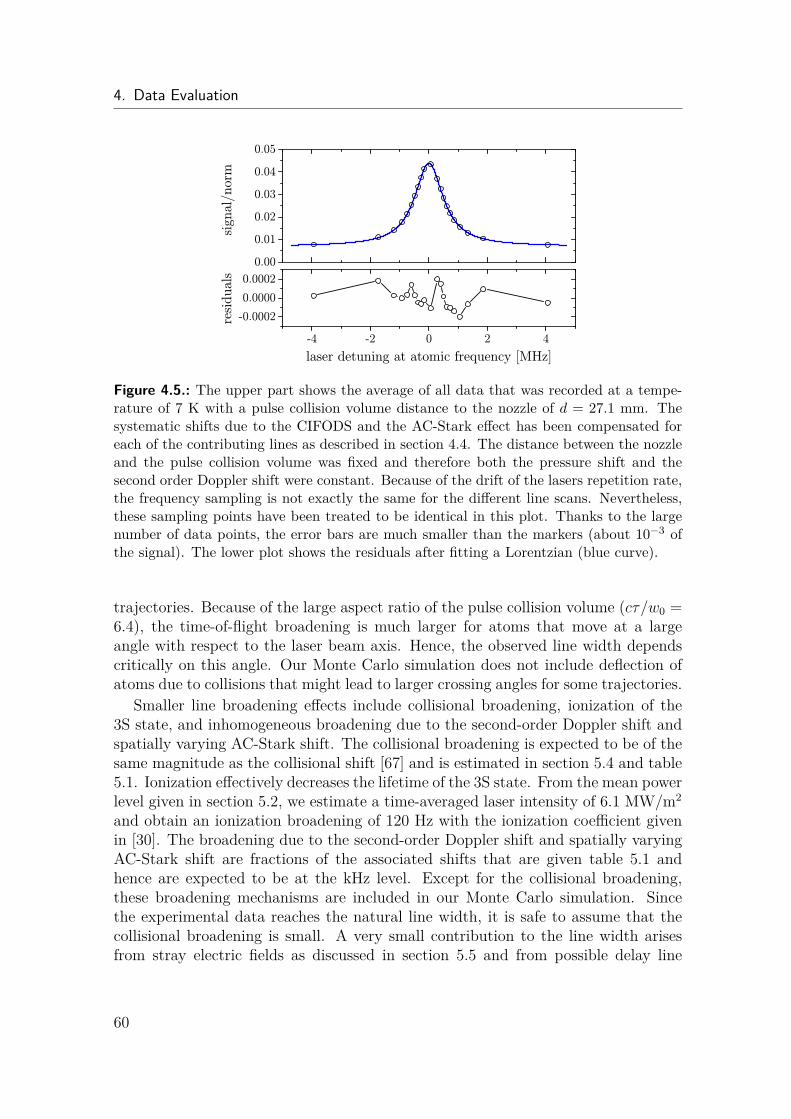
4. Data Evaluation
Figure 4.5.: The upper part shows the average of all data that was recorded at a tempe-rature of 7 K with a pulse collision volume distance to the nozzle of d = 27.1 mm. Thesystematic shifts due to the CIFODS and the AC-Stark effect has been compensated foreach of the contributing lines as described in section 4.4. The distance between the nozzleand the pulse collision volume was fixed and therefore both the pressure shift and thesecond order Doppler shift were constant. Because of the drift of the lasers repetition rate,the frequency sampling is not exactly the same for the different line scans. Nevertheless,these sampling points have been treated to be identical in this plot. Thanks to the largenumber of data points, the error bars are much smaller than the markers (about 10−3 ofthe signal). The lower plot shows the residuals after fitting a Lorentzian (blue curve).
trajectories. Because of the large aspect ratio of the pulse collision volume (cτ/w0 =6.4), the time-of-flight broadening is much larger for atoms that move at a largeangle with respect to the laser beam axis. Hence, the observed line width dependscritically on this angle. Our Monte Carlo simulation does not include deflection ofatoms due to collisions that might lead to larger crossing angles for some trajectories.
Smaller line broadening effects include collisional broadening, ionization of the3S state, and inhomogeneous broadening due to the second-order Doppler shift andspatially varying AC-Stark shift. The collisional broadening is expected to be of thesame magnitude as the collisional shift [67] and is estimated in section 5.4 and table5.1. Ionization effectively decreases the lifetime of the 3S state. From the mean powerlevel given in section 5.2, we estimate a time-averaged laser intensity of 6.1 MW/m2
and obtain an ionization broadening of 120 Hz with the ionization coefficient givenin [30]. The broadening due to the second-order Doppler shift and spatially varyingAC-Stark shift are fractions of the associated shifts that are given table 5.1 andhence are expected to be at the kHz level. Except for the collisional broadening,these broadening mechanisms are included in our Monte Carlo simulation. Sincethe experimental data reaches the natural line width, it is safe to assume that thecollisional broadening is small. A very small contribution to the line width arisesfrom stray electric fields as discussed in section 5.5 and from possible delay line
60
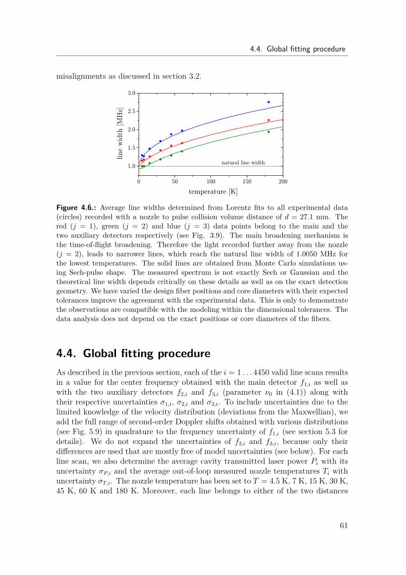
4.4. Global fitting procedure
misalignments as discussed in section 3.2.
Figure 4.6.: Average line widths determined from Lorentz fits to all experimental data(circles) recorded with a nozzle to pulse collision volume distance of d = 27.1 mm. Thered (j = 1), green (j = 2) and blue (j = 3) data points belong to the main and thetwo auxiliary detectors respectively (see Fig. 3.9). The main broadening mechanism isthe time-of-flight broadening. Therefore the light recorded further away from the nozzle(j = 2), leads to narrower lines, which reach the natural line width of 1.0050 MHz forthe lowest temperatures. The solid lines are obtained from Monte Carlo simulations us-ing Sech-pulse shape. The measured spectrum is not exactly Sech or Gaussian and thetheoretical line width depends critically on these details as well as on the exact detectiongeometry. We have varied the design fiber positions and core diameters with their expectedtolerances improve the agreement with the experimental data. This is only to demonstratethe observations are compatible with the modeling within the dimensional tolerances. Thedata analysis does not depend on the exact positions or core diameters of the fibers.
4.4. Global fitting procedureAs described in the previous section, each of the i = 1 . . . 4450 valid line scans resultsin a value for the center frequency obtained with the main detector f1,i as well aswith the two auxiliary detectors f2,i and f3,i (parameter ν0 in (4.1)) along withtheir respective uncertainties σ1,i, σ2,i and σ3,i. To include uncertainties due to thelimited knowledge of the velocity distribution (deviations from the Maxwellian), weadd the full range of second-order Doppler shifts obtained with various distributions(see Fig. 5.9) in quadrature to the frequency uncertainty of f1,i (see section 5.3 fordetails). We do not expand the uncertainties of f2,i and f3,i, because only theirdifferences are used that are mostly free of model uncertainties (see below). For eachline scan, we also determine the average cavity transmitted laser power Pi with itsuncertainty σP,i and the average out-of-loop measured nozzle temperatures Ti withuncertainty σT,i. The nozzle temperature has been set to T = 4.5 K, 7 K, 15 K, 30 K,45 K, 60 K and 180 K. Moreover, each line belongs to either of the two distances
61
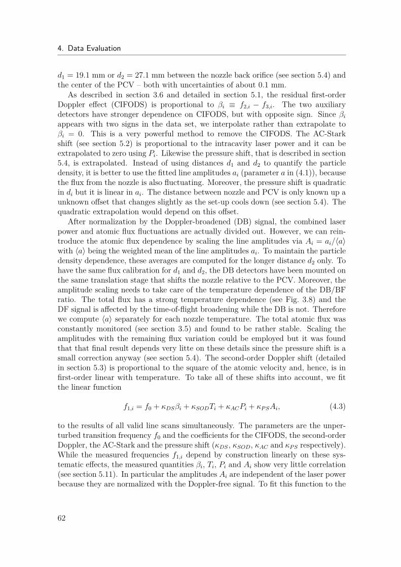
4. Data Evaluation
d1 = 19.1 mm or d2 = 27.1 mm between the nozzle back orifice (see section 5.4) andthe center of the PCV – both with uncertainties of about 0.1 mm.
As described in section 3.6 and detailed in section 5.1, the residual first-orderDoppler effect (CIFODS) is proportional to βi ≡ f2,i − f3,i. The two auxiliarydetectors have stronger dependence on CIFODS, but with opposite sign. Since βiappears with two signs in the data set, we interpolate rather than extrapolate toβi = 0. This is a very powerful method to remove the CIFODS. The AC-Starkshift (see section 5.2) is proportional to the intracavity laser power and it can beextrapolated to zero using Pi. Likewise the pressure shift, that is described in section5.4, is extrapolated. Instead of using distances d1 and d2 to quantify the particledensity, it is better to use the fitted line amplitudes ai (parameter a in (4.1)), becausethe flux from the nozzle is also fluctuating. Moreover, the pressure shift is quadraticin di but it is linear in ai. The distance between nozzle and PCV is only known up aunknown offset that changes slightly as the set-up cools down (see section 5.4). Thequadratic extrapolation would depend on this offset.
After normalization by the Doppler-broadened (DB) signal, the combined laserpower and atomic flux fluctuations are actually divided out. However, we can rein-troduce the atomic flux dependence by scaling the line amplitudes via Ai = ai/〈a〉with 〈a〉 being the weighted mean of the line amplitudes ai. To maintain the particledensity dependence, these averages are computed for the longer distance d2 only. Tohave the same flux calibration for d1 and d2, the DB detectors have been mounted onthe same translation stage that shifts the nozzle relative to the PCV. Moreover, theamplitude scaling needs to take care of the temperature dependence of the DB/BFratio. The total flux has a strong temperature dependence (see Fig. 3.8) and theDF signal is affected by the time-of-flight broadening while the DB is not. Thereforewe compute 〈a〉 separately for each nozzle temperature. The total atomic flux wasconstantly monitored (see section 3.5) and found to be rather stable. Scaling theamplitudes with the remaining flux variation could be employed but it was foundthat that final result depends very litte on these details since the pressure shift is asmall correction anyway (see section 5.4). The second-order Doppler shift (detailedin section 5.3) is proportional to the square of the atomic velocity and, hence, is infirst-order linear with temperature. To take all of these shifts into account, we fitthe linear function
f1,i = f0 + κDSβi + κSODTi + κACPi + κPSAi, (4.3)
to the results of all valid line scans simultaneously. The parameters are the unper-turbed transition frequency f0 and the coefficients for the CIFODS, the second-orderDoppler, the AC-Stark and the pressure shift (κDS, κSOD, κAC and κPS respectively).While the measured frequencies f1,i depend by construction linearly on these sys-tematic effects, the measured quantities βi, Ti, Pi and Ai show very little correlation(see section 5.11). In particular the amplitudes Ai are independent of the laser powerbecause they are normalized with the Doppler-free signal. To fit this function to the
62
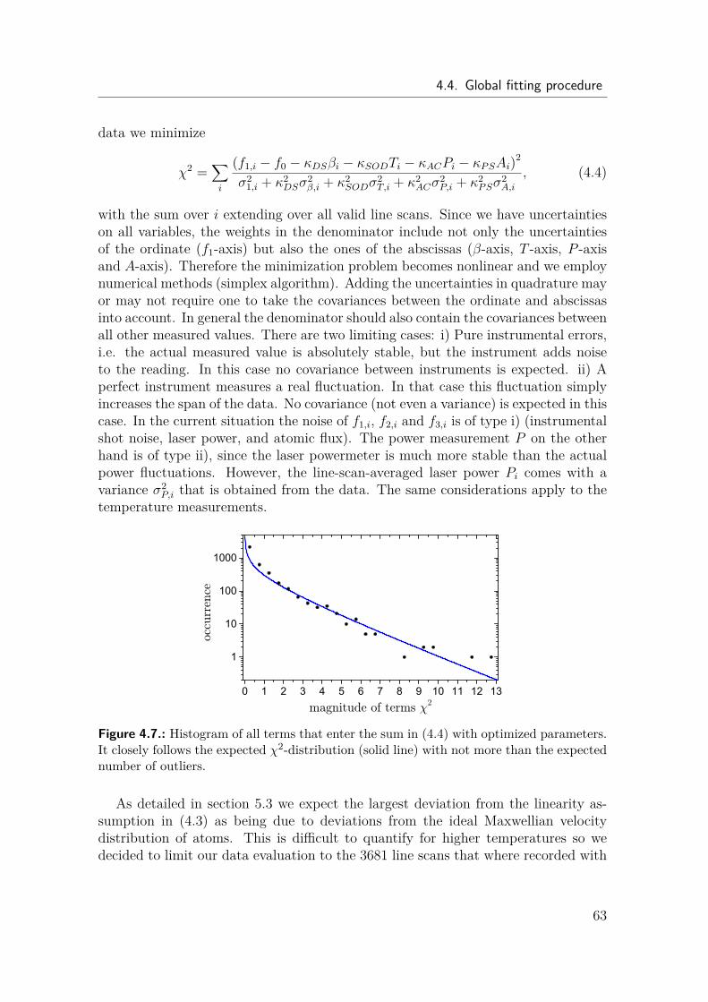
4.4. Global fitting procedure
data we minimize
χ2 =∑i
(f1,i − f0 − κDSβi − κSODTi − κACPi − κPSAi)2
σ21,i + κ2
DSσ2β,i + κ2
SODσ2T,i + κ2
ACσ2P,i + κ2
PSσ2A,i
, (4.4)
with the sum over i extending over all valid line scans. Since we have uncertaintieson all variables, the weights in the denominator include not only the uncertaintiesof the ordinate (f1-axis) but also the ones of the abscissas (β-axis, T -axis, P -axisand A-axis). Therefore the minimization problem becomes nonlinear and we employnumerical methods (simplex algorithm). Adding the uncertainties in quadrature mayor may not require one to take the covariances between the ordinate and abscissasinto account. In general the denominator should also contain the covariances betweenall other measured values. There are two limiting cases: i) Pure instrumental errors,i.e. the actual measured value is absolutely stable, but the instrument adds noiseto the reading. In this case no covariance between instruments is expected. ii) Aperfect instrument measures a real fluctuation. In that case this fluctuation simplyincreases the span of the data. No covariance (not even a variance) is expected in thiscase. In the current situation the noise of f1,i, f2,i and f3,i is of type i) (instrumentalshot noise, laser power, and atomic flux). The power measurement P on the otherhand is of type ii), since the laser powermeter is much more stable than the actualpower fluctuations. However, the line-scan-averaged laser power Pi comes with avariance σ2
P,i that is obtained from the data. The same considerations apply to thetemperature measurements.
Figure 4.7.: Histogram of all terms that enter the sum in (4.4) with optimized parameters.It closely follows the expected χ2-distribution (solid line) with not more than the expectednumber of outliers.
As detailed in section 5.3 we expect the largest deviation from the linearity as-sumption in (4.3) as being due to deviations from the ideal Maxwellian velocitydistribution of atoms. This is difficult to quantify for higher temperatures so wedecided to limit our data evaluation to the 3681 line scans that where recorded with
63
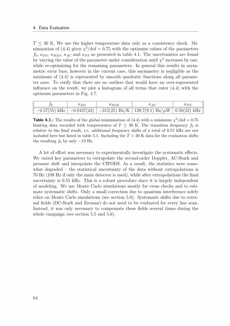
4. Data Evaluation
T ≤ 30 K. We use the higher temperature data only as a consistency check. Mi-nimization of (4.4) gives χ2/dof = 0.75 with the optimum values of the parametersf0, κDS, κSOD, κAC and κPS as presented in table 4.1. The uncertainties are foundby varying the value of the parameter under consideration until χ2 increases by one,while re-optimizing for the remaining parameters. In general this results in asym-metric error bars, however in the current case, this asymmetry is negligible as theminimum of (4.4) is represented by smooth quadratic functions along all parame-ter axes. To verify that there are no outliers that would have an over-representedinfluence on the result, we plot a histogram of all terms that enter (4.4) with theoptimum parameters in Fig. 4.7.
f0 κDS κSOD κAC κPS
−0.57(55) kHz −0.0437(43) −315(25) Hz/K 139.7(9.1) Hz/µW 0.58(22) kHz
Table 4.1.: The results of the global minimisation of (4.4) with a minimum χ2/dof = 0.75limiting data recorded with temperatures of T ≤ 30 K. The transition frequency f0 isrelative to the final result, i.e. additional frequency shifts of a total of 0.57 kHz are notincluded here but listed in table 5.1. Including the T > 30 K data for the evaluation shiftsthe resulting f0 by only −13 Hz.
A lot of effort was necessary to experimentally investigate the systematic effects.We varied key parameters to extrapolate the second-order Doppler, AC-Stark andpressure shift and interpolate the CIFODS. As a result, the statistics were some-what degraded – the statistical uncertainty of the data without extrapolations is70 Hz (108 Hz if only the main detector is used), while after extrapolations the finaluncertainty is 0.55 kHz. This is a robust procedure since it is largely independentof modeling. We use Monte Carlo simulations mostly for cross checks and to esti-mate systematic shifts. Only a small correction due to quantum interference solelyrelies on Monte Carlo simulations (see section 5.8). Systematic shifts due to exter-nal fields (DC-Stark and Zeeman) do not need to be evaluated for every line scan.Instead, it was only necessary to compensate these fields several times during thewhole campaign (see section 5.5 and 5.6).
64
5. Systematic Uncertainties Analysis
5.1. Chirp induced residual first-order Doppler shiftTwo-photon transitions allow for the suppression of the first-order Doppler shift.However, in direct frequency comb two-photon spectroscopy a residual chirp inducedfirst-order Doppler shift (CIFODS) may emerge [21]. In our case, the divergence ofthe atomic beam, together with a small frequency chirp of the laser pulses causes thisshift and is explained below. For an approximate analytical model we are assuming aGaussian pulse shape because it leads to compact expression, while we can readily useany pulse shape for the Monte Carlo simulations. Consider two counter-propagatinglinearly chirped pulse trains,
E± = E0∑n
exp(−(1 + ib)(t− ntrep ± z/c)2
τ2 − x2 + y2
w(z)2 − iωct∓ ikcz ± i arctan(z/zR))
(5.1)with the position along the propagation direction z, the radial position x, y, time t, theusual beam radius w(z) = w0
√1 + (z/zR)2, the Rayleigh length zR = kzw
20/2, and
the laser beam waist w0. The sum extends over the forward (E+) and backward (E−)propagating pulses with the repetition time trep = 1/frep, pulse duration τ (FWHMintensity T1/2 = τ
√2 ln(2)), carrier frequency ωc = ckc, and the dimensionless chirp
parameter b. We choose a pure frequency domain chirp (in contrast to a time domainchirp, see [26] with a = 1), because this is what we expect with ps pulses andthe dominating self-phase modulation. The reversing sign of the z/c term is givenby requiring the same temporal color sequence of the reflected pulses. The Rabifrequency of the (almost) Doppler-free transition amplitude is proportional to theproduct of the two fields E+E−[30]
Ω(t) =( 2π
)3/2 8πβgePLfrepτw(z)2
∑n
exp(−2(1+ib)
[(t−ntrep)2
τ2 + z2
c2τ2
]− 2x
2 + y2
w(z)2 − i2ωct),
(5.2)where we consider only one PCV close to z = 0 and are therefore left with onlyone sum. One can also observe that a power imbalance between the forward andbackward propagating pulses (|E+| , |E−|) does not lead to a Doppler shift butonly a decrease in the Doppler-free transition amplitude. The Rabi frequency ofthe Doppler-broadened component is proportional to E+E
∗−. The laser power PL
is measured in one propagation direction only and the parameter βge is given insection 2.5. The term that oscillates with twice the carrier frequency is removedwith the rotating wave approximation. For an atomic trajectory along the z-axiswith z(t) = z0 + vzt, one sees that the usual first-order Doppler term kcvz is absent.
65
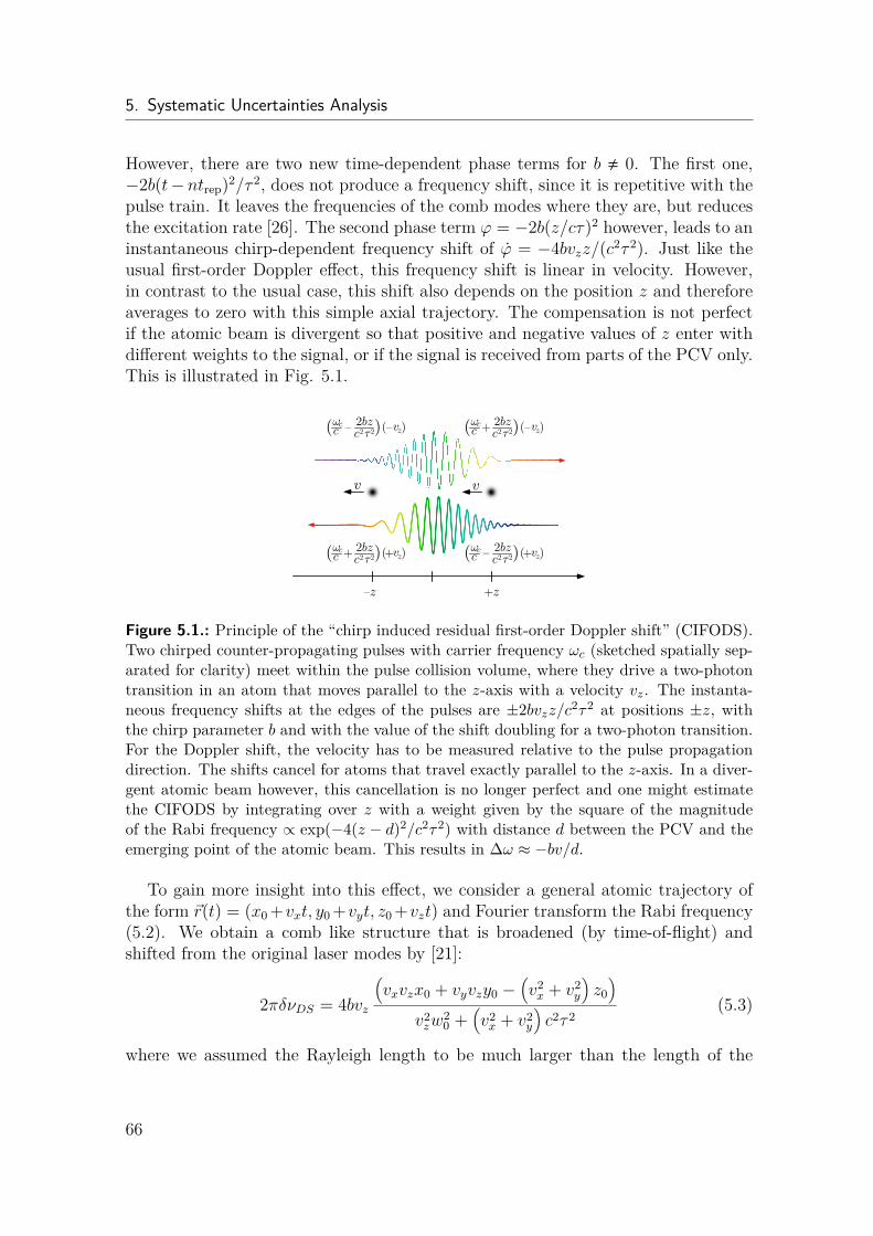
5. Systematic Uncertainties Analysis
However, there are two new time-dependent phase terms for b , 0. The first one,−2b(t−ntrep)2/τ 2, does not produce a frequency shift, since it is repetitive with thepulse train. It leaves the frequencies of the comb modes where they are, but reducesthe excitation rate [26]. The second phase term ϕ = −2b(z/cτ)2 however, leads to aninstantaneous chirp-dependent frequency shift of ϕ = −4bvzz/(c2τ 2). Just like theusual first-order Doppler effect, this frequency shift is linear in velocity. However,in contrast to the usual case, this shift also depends on the position z and thereforeaverages to zero with this simple axial trajectory. The compensation is not perfectif the atomic beam is divergent so that positive and negative values of z enter withdifferent weights to the signal, or if the signal is received from parts of the PCV only.This is illustrated in Fig. 5.1.
v
ωcτ2— )( )v— zc 2( 2bz
c
v
— +zz
ωcτ2+ )( )v+ zc 2( 2bz
c
ωcτ2+ )( )v— zc 2( 2bz
c
ωcτ2— )( )v+ zc 2( 2bz
c
Figure 5.1.: Principle of the “chirp induced residual first-order Doppler shift” (CIFODS).Two chirped counter-propagating pulses with carrier frequency ωc (sketched spatially sep-arated for clarity) meet within the pulse collision volume, where they drive a two-photontransition in an atom that moves parallel to the z-axis with a velocity vz. The instanta-neous frequency shifts at the edges of the pulses are ±2bvzz/c2τ2 at positions ±z, withthe chirp parameter b and with the value of the shift doubling for a two-photon transition.For the Doppler shift, the velocity has to be measured relative to the pulse propagationdirection. The shifts cancel for atoms that travel exactly parallel to the z-axis. In a diver-gent atomic beam however, this cancellation is no longer perfect and one might estimatethe CIFODS by integrating over z with a weight given by the square of the magnitudeof the Rabi frequency ∝ exp(−4(z − d)2/c2τ2) with distance d between the PCV and theemerging point of the atomic beam. This results in ∆ω ≈ −bv/d.
To gain more insight into this effect, we consider a general atomic trajectory ofthe form ~r(t) = (x0 +vxt, y0 +vyt, z0 +vzt) and Fourier transform the Rabi frequency(5.2). We obtain a comb like structure that is broadened (by time-of-flight) andshifted from the original laser modes by [21]:
2πδνDS = 4bvz
(vxvzx0 + vyvzy0 −
(v2x + v2
y
)z0)
v2zw
20 +
(v2x + v2
y
)c2τ 2
(5.3)
where we assumed the Rayleigh length to be much larger than the length of the
66
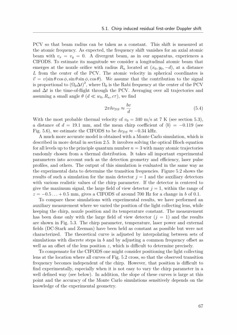
5.1. Chirp induced residual first-order Doppler shift
PCV so that beam radius can be taken as a constant. This shift is measured atthe atomic frequency. As expected, the frequency shift vanishes for an axial atomicbeam with vx = vy = 0. A divergent beam, as in our apparatus, experiences aCIFODS. To estimate its magnitude we consider a longitudinal atomic beam thatemerges at the nozzle orifice with radius Rn located at (x0, y0,−d), at a distanceL from the center of the PCV. The atomic velocity in spherical coordinates is~v = v(sin θ cosφ, sin θ sinφ, cos θ). We assume that the contribution to the signalis proportional to (Ω0∆t)2, where Ω0 is the Rabi frequency at the center of the PCVand ∆t is the time-of-flight through the PCV. Averaging over all trajectories andassuming a small angle θ (d w0, Rn, cτ), we find
2πδνDS ≈bv
d(5.4)
With the most probable thermal velocity of v0 = 340 m/s at 7 K (see section 5.3),a distance of d = 19.1 mm, and the mean chirp coefficient of 〈b〉 = −0.119 (seeFig. 5.6), we estimate the CIFODS to be δνDS ≈ −0.34 kHz.
A much more accurate model is obtained with a Monte Carlo simulation, which isdescribed in more detail in section 2.5. It involves solving the optical Bloch equationfor all levels up to the principle quantum number n = 3 with many atomic trajectoriesrandomly chosen from a thermal distribution. It takes all important experimentalparameters into account such as the detection geometry and efficiency, laser pulseprofiles, and others. The output of this simulation is evaluated in the same way asthe experimental data to determine the transition frequencies. Figure 5.2 shows theresults of such a simulation for the main detector j = 1 and the auxiliary detectorswith various realistic values of the chirp parameter. If the detector is centered togive the maximum signal, the large field of view detector j = 1, within the range ofz = −0.5 . . .+ 0.5 mm, gives a CIFODS of around 700 Hz for a change in b of 0.1.
To compare these simulations with experimental results, we have performed anauxiliary measurement where we varied the position of the light collecting lens, whilekeeping the chirp, nozzle position and its temperature constant. The measurementhas been done only with the large field of view detector (j = 1) and the resultsare shown in Fig. 5.3. The chirp parameter, temperature, laser power and externalfields (DC-Stark and Zeeman) have been held as constant as possible but were notcharacterized. The theoretical curve is adjusted by interpolating between sets ofsimulations with discrete steps in b and by adjusting a common frequency offset aswell as an offset of the lens position z, which is difficult to determine precisely.
To compensate for the CIFODS one might consider positioning the light collectinglens at the location where all curves of Fig. 5.2 cross, so that the observed transitionfrequency becomes independent of the chirp. However, that position is difficult tofind experimentally, especially when it is not easy to vary the chirp parameter in awell defined way (see below). In addition, the slope of these curves is large at thispoint and the accuracy of the Monte Carlo simulations sensitively depends on theknowledge of the experimental geometry.
67
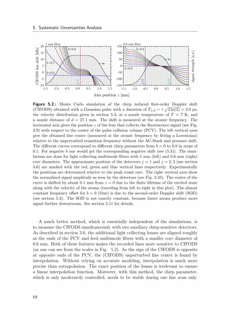
5. Systematic Uncertainties Analysis
Figure 5.2.: Monte Carlo simulation of the chirp induced first-order Doppler shift(CIFODS) obtained with a Gaussian pulse with a duration of T1/2 = τ
√2 ln(2) = 2.0 ps,
the velocity distribution given in section 5.3, at a nozzle temperature of T = 7 K, anda nozzle distance of d = 27.1 mm. The shift is measured at the atomic frequency. Thehorizontal axis gives the position z of the lens that collects the fluorescence signal (see Fig.3.9) with respect to the center of the pulse collision volume (PCV). The left vertical axesgive the obtained line center (measured at the atomic frequency by fitting a Lorentzian)relative to the unperturbed transition frequency without the AC-Stark and pressure shift.The different curves correspond to different chirp parameters from b = 0 to 0.8 in steps of0.1. For negative b one would get the corresponding negative shift (see (5.3)). The simu-lations are done for light collecting multimode fibers with 1 mm (left) and 0.6 mm (right)core diameters. The approximate position of the detectors j = 1 and j = 2, 3 (see section3.6) are marked with the red, green and blue vertical lines respectively. Experimentallythe positions are determined relative to the peak count rate. The right vertical axes showthe normalized signal amplitude as seen by the detectors (see Fig. 3.10). The center of thecurve is shifted by about 0.1 mm from z = 0 due to the finite lifetime of the excited statealong with the velocity of the atoms (traveling from left to right in this plot). The almostconstant frequency offset for b = 0 (blue) is due to the second-order Doppler shift (SOD)(see section 5.3). The SOD is not exactly constant, because faster atoms produce moresignal further downstream. See section 5.11 for details.
A much better method, which is essentially independent of the simulations, isto measure the CIFODS simultaneously with two auxiliary chirp-sensitive detectors.As described in section 3.6, the additional light collecting lenses are aligned roughlyat the ends of the PCV and feed multimode fibers with a smaller core diameter of0.6 mm. Both of these features makes the recorded lines more sensitive to CIFODS(as one can see from the scales in Fig. 5.2). As the sign of the CIFODS is oppositeat opposite ends of the PCV, the (CIFODS) unperturbed line center is found byinterpolation. Without relying on accurate modeling, interpolation is much moreprecise than extrapolation. The exact position of the lenses is irrelevant to ensurea linear interpolation function. Moreover, with this method, the chirp parameter,which is only moderately controlled, needs to be stable during one line scan only.
68
5.1. Chirp induced residual first-order Doppler shift
Figure 5.3.: Experimental determination of the chirp induced residual first-order Dopplershift (CIFODS) measured at the atomic frequency and recorded at a nozzle temperature of8 K. We attempted to keep the other systematic frequency shifts as constant as possible,but they were not characterized. Therefore, the CIFODS shown here is relative to anunknown offset. The error bars are obtained from a weighted average of lines scans thatare assumed subject to shot noise only. This plot is to be compared with the theoreticalmodel presented in Fig. 5.2. The latter is adjusted for the chirp parameter b, an offset ofthe lens position z, as well as a frequency offset. The best fitting (χ2/dof = 0.55) chirpcoefficient is b = 0.5(1), which corresponds to a CIFODS of 3.5 kHz with a centered lens.
Further, as explained below, we do not even need to know its value. As seen at theright hand side of Fig. 5.2, the CIFODS at z = −0.5 mm is about 8 kHz for a changeof ∆b = 0.1. At the opposite side at z = 0.7 mm (note that the signal maximizesat z = 0.1 mm), the dependence is slightly smaller (6.5 kHz per 0.1 change of thechirp parameter). For example, by placing the main detector at z = 0.1 mm, andthe auxiliary detectors at z = −0.5 mm and at z = 0.7 mm, the frequency differenceobserved by the two auxiliary detectors is about 15 kHz for a chirp of b = 0.1 withthe 0.6 mm fibers. This is roughly 10 times larger than for the main detector.
Even though the CIFODS is a complicated function of the position z, for fixed zit is very linear as a function of the chirp parameter b as the simulations in Fig. 5.4show. This can be exploited with a linear interpolation method for its compensation.For this purpose we first express the observed transition frequencies fj,i obtained withthe detectors j = 1, 2, 3 and the line scan i in terms of the CIFODS unperturbedtransition frequency f0 and three (unknown) coefficients αj:
f1,i = f0 + α1bi f2,i = f0 + α2bi f3,i = f0 + α3bi. (5.5)
Then these equations are rearranged in the following way
f1,i = f0 + α1
α2 − α3(f2,i − f3,i) = f0 + κDS (f2,i − f3,i) = f0 + κDSβi (5.6)
which gives us the linear interpolation model that has been used in section 4.4 withβi ≡ f2,i − f3,i ∝ bi. The actual value of the chirp parameter is not required to find
69
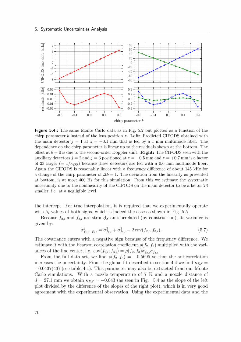
5. Systematic Uncertainties Analysis
Figure 5.4.: The same Monte Carlo data as in Fig. 5.2 but plotted as a function of thechirp parameter b instead of the lens position z. Left: Predicted CIFODS obtained withthe main detector j = 1 at z = +0.1 mm that is fed by a 1 mm multimode fiber. Thedependence on the chirp parameter is linear up to the residuals shown at the bottom. Theoffset at b = 0 is due to the second-order Doppler shift. Right: The CIFODS seen with theauxiliary detectors j = 2 and j = 3 positioned at z = −0.5 mm and z = +0.7 mm is a factorof 23 larger (= 1/κDS) because these detectors are fed with a 0.6 mm multimode fiber.Again the CIFODS is reasonably linear with a frequency difference of about 145 kHz fora change of the chirp parameter of ∆b = 1. The deviation from the linearity as presentedat bottom, is at most 400 Hz for this simulation. From this we estimate the systematicuncertainty due to the nonlinearity of the CIFODS on the main detector to be a factor 23smaller, i.e. at a negligible level.
the intercept. For true interpolation, it is required that we experimentally operatewith βi values of both signs, which is indeed the case as shown in Fig. 5.5.
Because f2,i and f3,i are strongly anticorrelated (by construction), its variance isgiven by:
σ2f2,i−f3,i
= σ2f2,i
+ σ2f3,i− 2 cov(f2,i, f3,i). (5.7)
The covariance enters with a negative sign because of the frequency difference. Weestimate it with the Pearson correlation coefficient ρ(f2, f3) multiplied with the vari-ances of the line center, i.e. cov(f2,i, f3,i) = ρ(f2, f3)σf2,iσf3,i .
From the full data set, we find ρ(f2, f3) = −0.5695 so that the anticorrelationincreases the uncertainty. From the global fit described in section 4.4 we find κDS =−0.0437(43) (see table 4.1). This parameter may also be extracted from our MonteCarlo simulations. With a nozzle temperature of 7 K and a nozzle distance ofd = 27.1 mm we obtain κDS = −0.043 (as seen in Fig. 5.4 as the slope of the leftplot divided by the difference of the slopes of the right plot), which is in very goodagreement with the experimental observation. Using the experimental data and the
70
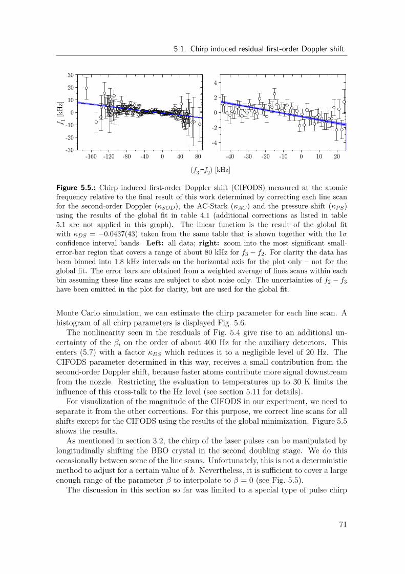
5.1. Chirp induced residual first-order Doppler shift
−
Figure 5.5.: Chirp induced first-order Doppler shift (CIFODS) measured at the atomicfrequency relative to the final result of this work determined by correcting each line scanfor the second-order Doppler (κSOD), the AC-Stark (κAC) and the pressure shift (κPS)using the results of the global fit in table 4.1 (additional corrections as listed in table5.1 are not applied in this graph). The linear function is the result of the global fitwith κDS = −0.0437(43) taken from the same table that is shown together with the 1σconfidence interval bands. Left: all data; right: zoom into the most significant small-error-bar region that covers a range of about 80 kHz for f3 − f2. For clarity the data hasbeen binned into 1.8 kHz intervals on the horizontal axis for the plot only – not for theglobal fit. The error bars are obtained from a weighted average of lines scans within eachbin assuming these line scans are subject to shot noise only. The uncertainties of f2 − f3have been omitted in the plot for clarity, but are used for the global fit.
Monte Carlo simulation, we can estimate the chirp parameter for each line scan. Ahistogram of all chirp parameters is displayed Fig. 5.6.
The nonlinearity seen in the residuals of Fig. 5.4 give rise to an additional un-certainty of the βi on the order of about 400 Hz for the auxiliary detectors. Thisenters (5.7) with a factor κDS which reduces it to a negligible level of 20 Hz. TheCIFODS parameter determined in this way, receives a small contribution from thesecond-order Doppler shift, because faster atoms contribute more signal downstreamfrom the nozzle. Restricting the evaluation to temperatures up to 30 K limits theinfluence of this cross-talk to the Hz level (see section 5.11 for details).
For visualization of the magnitude of the CIFODS in our experiment, we need toseparate it from the other corrections. For this purpose, we correct line scans for allshifts except for the CIFODS using the results of the global minimization. Figure 5.5shows the results.
As mentioned in section 3.2, the chirp of the laser pulses can be manipulated bylongitudinally shifting the BBO crystal in the second doubling stage. We do thisoccasionally between some of the line scans. Unfortunately, this is not a deterministicmethod to adjust for a certain value of b. Nevertheless, it is sufficient to cover a largeenough range of the parameter β to interpolate to β = 0 (see Fig. 5.5).
The discussion in this section so far was limited to a special type of pulse chirp
71
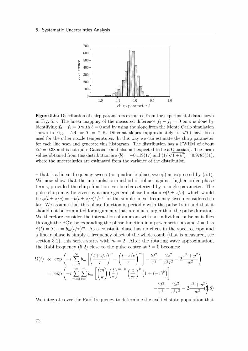
5. Systematic Uncertainties Analysis
Figure 5.6.: Distribution of chirp parameters extracted from the experimental data shownin Fig. 5.5. The linear mapping of the measured difference f3 − f2 = 0 on b is done byidentifying f3− f2 = 0 with b = 0 and by using the slope from the Monte Carlo simulationshown in Fig. 5.4 for T = 7 K. Different slopes (approximately ∝
√T ) have been
used for the other nozzle temperatures. In this way we can estimate the chirp parameterfor each line scan and generate this histogram. The distribution has a FWHM of about∆b = 0.38 and is not quite Gaussian (and also not expected to be a Gaussian). The meanvalues obtained from this distribution are 〈b〉 = −0.119(17) and 〈1/
√1 + b2〉 = 0.9783(31),
where the uncertainties are estimated from the variance of the distribution.
– that is a linear frequency sweep (or quadratic phase sweep) as expressed by (5.1).We now show that the interpolation method is robust against higher order phaseterms, provided the chirp function can be characterized by a single parameter. Thepulse chirp may be given by a more general phase function φ(t± z/c), which wouldbe φ(t± z/c) = −b(t± z/c)2/τ 2 for the simple linear frequency sweep considered sofar. We assume that this phase function is periodic with the pulse train and that itshould not be computed for arguments that are much larger than the pulse duration.We therefore consider the interaction of an atom with an individual pulse as it fliesthrough the PCV by expanding the phase function in a power series around t = 0 asφ(t) = ∑
m = bm(t/τ)m. As a constant phase has no effect in the spectroscopy anda linear phase is simply a frequency offset of the whole comb (that is measured, seesection 3.1), this series starts with m = 2. After the rotating wave approximation,the Rabi frequency (5.2) close to the pulse center at t = 0 becomes:
Ω(t) ∝ exp(−i
∞∑m=2
bm
[(t+z/cτ
)m+(t−z/cτ
)m]− 2t2τ 2 −
2z2
c2τ 2 − 2x2 + y2
w2
)
= exp(−i
∞∑m=2
m∑k=0
bm
[(m
k
)(t
τ
)m−k ( zcτ
)k (1 + (−1)k
)]
−2t2τ 2 −
2z2
c2τ 2 − 2x2 + y2
w2
)(5.8)
We integrate over the Rabi frequency to determine the excited state population that
72
5.1. Chirp induced residual first-order Doppler shift
is added per pulse:a(z) =
∫ +nτ
−nτΩ(t)dt. (5.9)
Here nτ is some multiple of the pulse duration. For the simulations described inmore detail in section 2.5, we use n = 3 as a good approximation. Increasing n didnot yield a significant change of the results. To further simplify the computations,we assume that the atom position is fixed during the pulses, but account for itsmotion between the pulses. To justify this approach, we note from (5.8) that thephase change of Ω(t) is proportional to (t/τ)2 to leading order – within a given pulse,we have |t/τ | . n, whereas between two pulses this number is more than 3 orders ofmagnitude larger.
Any chirp-induced Doppler shift can now be understood as a phase change of a(z)with position:
δνDS = vz2π
∂ arg [a(z)]∂z
. (5.10)
The phase term of the integral (5.9) extends over an odd function for odd m−k andhence vanishes. Therefore only even m − k contribute to the chirp, and since onlyeven k occur, m must be an even number as well.
Our main source of chirp is due to self-phase modulation within the doublingcrystals (see section 3.2). For this case, the phase function, plotted in Fig. 3.4, isgiven by:
φ(t) = φ0e−2t2/τ2 = φ0
(1− 2t2
τ 2 + 2t4τ 4 −
4t63τ 6 + . . .
). (5.11)
Here, the odd terms are not even present and do not need to be suppressed by the two-photon excitation scheme. The additional higher-order terms give rise to a differentCIFODS so that the curves in Fig. 5.2 would need to be modified. Nevertheless,we expect that the frequency shift is in first-order linear in the new parameter φ0,similar to Fig. 5.4. In addition, the three detectors will obtain different CIFODS,which is in our geometry always minimal for the detector j = 1 that has the largestfield of view. With these assumptions we can define new (unknown) coefficients α′j:
f1,i = f0 + α′1φ0,i f2,i = f0 + α′2φ0,i f3,i = f0 + α′3φ0,i, (5.12)
which is in complete analogy to (5.5), and results in the same interpolation formula(5.6). It should be noted that this argument can be extended to a more generalcase of phase functions where the coefficients on the right hand side of (5.11) havedifferent values. We do not expect additional systematic CIFODS effects as long asthe relative size of the coefficients in that power series do not change between thelines scans and the chirp can be described by only one varying parameter, φ0,i.
With multiple mechanisms that can lead to a chirp, one might be in the regimeof a “multi-parameter CIFODS”. In this case the coefficients in the power series maychange simultaneously and independently. This may happen for example when themode locked laser contributes a linear chirp b that adds to the chirp that is generated
73
5. Systematic Uncertainties Analysis
by self-phase modulation within the doubling crystals. From the experiment andsimulations we know that the CIFODS we observe corresponds to a linear chirp inthe range of b ≈ −0.5 . . . 0.5. Further we know that most of our chirp is causedby self-phase modulation, so that the coefficient of the next order term, t4/τ 4, isat most as large as the coefficient of the first term. To estimate the associatedsystematic shift we ran Monte Carlo simulations (see section 2.5) with a phase profileφ(t) = b2t
2/τ 2 + b4t4/τ 4, where the coefficients are varied within the ranges of b2 =
0, 0.1, 0.2, . . . 0.9 and b4 = −0.4, 0.2, 0, 0.2, 0.4. By evaluating all combinations ofcoefficients with the interpolation method, we find a maximum shift of ±0.1 kHz.This possible systematic uncertainty is included in the final error budget shown intable 5.1.
5.2. AC-Stark shiftThe AC-Stark effect can be computed analytically for atomic hydrogen. Both theground state and the excited state are shifted by the local laser intensity I(~r) ac-cording to
δνAC = 2 (βAC(3S)− βAC(1S)) I(~r) = 2.565902× 10⁻⁴ HzW/m2 I(~r) (5.13)
with the notation and values given in [30]. Again, the shift is measured at the atomicfrequency (102.5 nm). The intensity is meant to correspond to the energy flow oflaser power in one direction only – hence, the factor of two in the above equation.The coefficients βAC have been computed for a linearly polarized continuous-wavelaser field. They can be used without modification for our purpose, as the σ+/σ−counter-propagating laser beams produce a linear polarization everywhere. The li-near polarization direction forms a helix in space. This helix alternates between twoconfigurations as σ+/σ− pulses alternate their directions every second pulse colli-sion event. Despite this complication the laser polarization that the atoms see islinear at each instant of time [63]. Moreover the AC-Stark shift of two-photon directfrequency comb spectroscopy is determined by the time-averaged intensity, not themuch larger peak intensity of the corresponding pulse train [43]. Therefore, I(~r)in (5.13) refers to the time-averaged intensity that is readily measured with a laserpowermeter. Averaging the laser intensity radially, we obtain an estimation for theAC-Stark shift of
〈I〉 = 2P/T2
πw20, (5.14)
where w0 = 80 µm is the laser waist radius, P = PLT2 is the time-averaged laserpower measured after the 205 nm enhancement cavity (see “PM” in Fig. 3.1)and T2 = 5.4 × 10⁻⁴ is the transmission of the back reflecting mirror (see sec-tion 3.4). With these numbers we obtain an approximate AC-Stark coefficient ofκAC = 47 Hz/µW from (5.13) and (5.14). From a Monte Carlo simulation, that
74
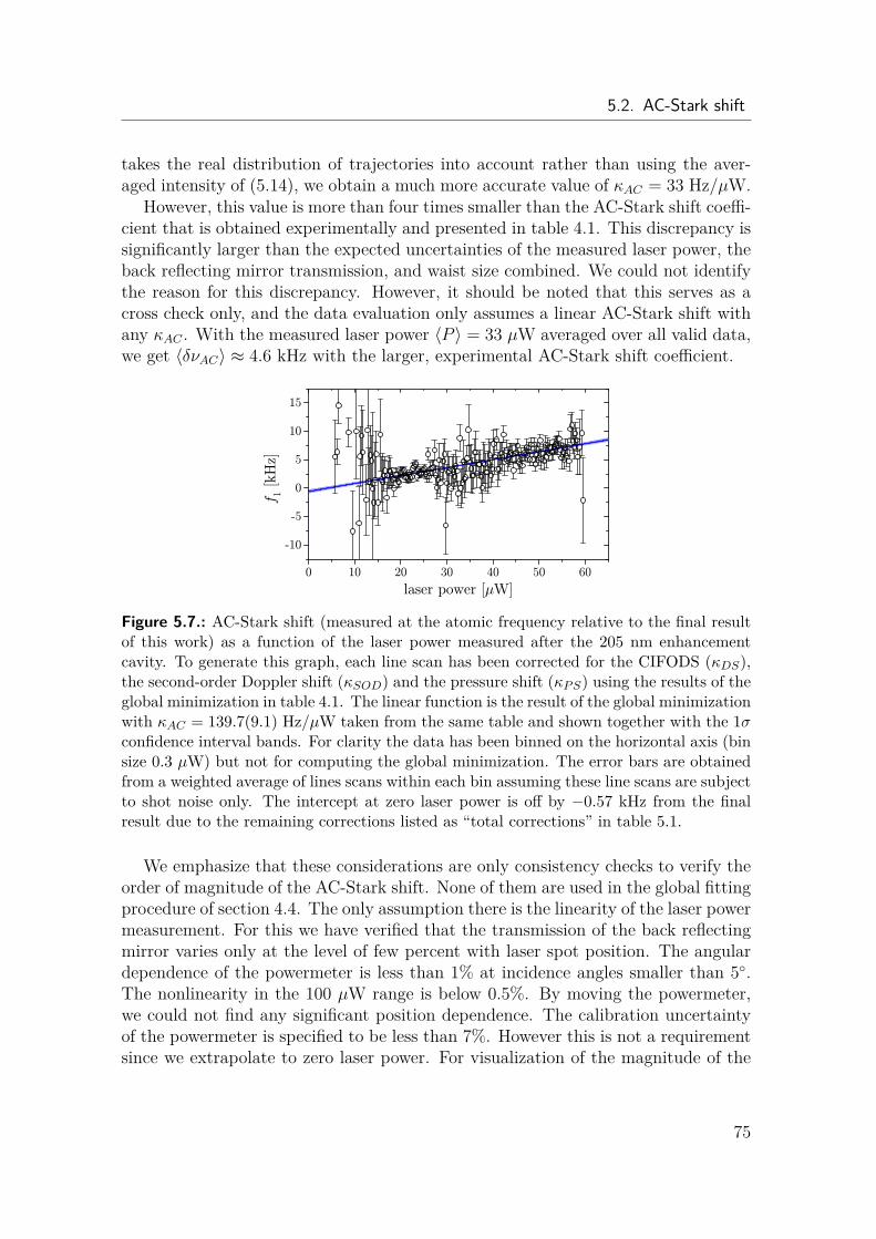
5.2. AC-Stark shift
takes the real distribution of trajectories into account rather than using the aver-aged intensity of (5.14), we obtain a much more accurate value of κAC = 33 Hz/µW.
However, this value is more than four times smaller than the AC-Stark shift coeffi-cient that is obtained experimentally and presented in table 4.1. This discrepancy issignificantly larger than the expected uncertainties of the measured laser power, theback reflecting mirror transmission, and waist size combined. We could not identifythe reason for this discrepancy. However, it should be noted that this serves as across check only, and the data evaluation only assumes a linear AC-Stark shift withany κAC . With the measured laser power 〈P 〉 = 33 µW averaged over all valid data,we get 〈δνAC〉 ≈ 4.6 kHz with the larger, experimental AC-Stark shift coefficient.
Figure 5.7.: AC-Stark shift (measured at the atomic frequency relative to the final resultof this work) as a function of the laser power measured after the 205 nm enhancementcavity. To generate this graph, each line scan has been corrected for the CIFODS (κDS),the second-order Doppler shift (κSOD) and the pressure shift (κPS) using the results of theglobal minimization in table 4.1. The linear function is the result of the global minimizationwith κAC = 139.7(9.1) Hz/µW taken from the same table and shown together with the 1σconfidence interval bands. For clarity the data has been binned on the horizontal axis (binsize 0.3 µW) but not for computing the global minimization. The error bars are obtainedfrom a weighted average of lines scans within each bin assuming these line scans are subjectto shot noise only. The intercept at zero laser power is off by −0.57 kHz from the finalresult due to the remaining corrections listed as “total corrections” in table 5.1.
We emphasize that these considerations are only consistency checks to verify theorder of magnitude of the AC-Stark shift. None of them are used in the global fittingprocedure of section 4.4. The only assumption there is the linearity of the laser powermeasurement. For this we have verified that the transmission of the back reflectingmirror varies only at the level of few percent with laser spot position. The angulardependence of the powermeter is less than 1% at incidence angles smaller than 5.The nonlinearity in the 100 µW range is below 0.5%. By moving the powermeter,we could not find any significant position dependence. The calibration uncertaintyof the powermeter is specified to be less than 7%. However this is not a requirementsince we extrapolate to zero laser power. For visualization of the magnitude of the
75
5. Systematic Uncertainties Analysis
AC-Stark shift in our experiment, we need to separate it from the other corrections.For this purpose we correct all line scans for all shifts except for the AC-Stark shiftusing the results of the global minimization – as was also done for the CIFODS.Figure 5.7 shows the result.
We also considered the possibility of a higher-order and hence nonlinear contri-bution to the AC-Stark shift. The experimental data shown in Fig. 5.7 does notexclude this possibility. In perturbation theory, the AC-Stark shift has only evenorders. The largest close-to-resonant contribution is due to the two-photon couplingof the 3S and 3D states. This effect can take place via the excitation paths 3S →nP → 3D → n′P → 3S with intermediate states nP, 3D and n′P, where n and n′
are summed over all bound and continuum states. For these paths, we derive thefrequency shift with fourth-order perturbation theory given by
δν(4)AC ≈
(ωrτ)2
2
(eE0
6~
)4(S+ − S−)2 ∑
Dn1,n2
e−(n21+n2
2)(ωrτ/2)2
ω3D,3S − (n1 − n2)ωr, (5.15)
whereS± ≡
∑n
µ3S,nP µnP,3D
ωnP,3S ± ωc. (5.16)
Here, the µ are the corresponding dipole matrix elements (see [57]), ωc is the combcarrier frequency, ωr is the repetition rate, and the other labeled ω are the cor-responding transition frequencies. While there are no resonances in (5.16), thereare close-to-resonant contributions in (5.15) because our frequency comb is widerthan the 3S-3D splitting. The sum extends over the 3D levels (fine and hyperfine)and two mode numbers of the frequency comb n1 and n2. With the mode spacingωr = 2π× 315.2 MHz, we find that no mode combination are closer than 7 times thenatural line width of the 3D level (10.3 MHz), so we do not include an imaginarydamping constant. By evaluating (5.15) with a peak field of E0 = 2.6 MV/m2, whichcorresponds to the mean experimental conditions, we find that this shift is much lessthan 1 Hz [63], and thus negligible.
The 2.4 GHz discharge that is used for dissociating hydrogen molecules into atoms(see section 3.4) might also give rise to a Stark shift. The discharge is locatedoutside the vacuum system (see Fig. 3.6 and Fig. 3.7) and is therefore shielded bythe vacuum vessel. An additional shield is provided by the fiber mount of the DFdetector assembly that also contains the compensation electrodes (see Fig. 5.14).The microwave electric field strength ERF at the position of the atoms has beenestimated to be around 0.3 V/m in a similar double shielded apparatus [64]. Thedominant contribution to this AC-Stark shift is due the coupling of the 3S state tothe 3P3/2 with a level separation of 2.93 GHz is given by
δνRFAC =
(µ3S,3PERF
2h
)2 12.93 GHz± 2.4 GHz (5.17)
76
5.3. Second-order Doppler shift
where the counter-rotating terms with the two signs have to be added. Assuminglinear polarization and µ3S,3P = 6ea0 for the 3S(F =1,M=0)→ 3P3/2(F =2,M=0)component we obtain δνRF
AC = 1.2 Hz.Another source for an AC-Stark shift is the black body radiation. The room
temperature (T = 300 K) black body shift of the 1S-3S centroid has been computedto −9.06 Hz [65]. This serves as a upper limit as parts of the structure surroundingthe PCV are certainly below room temperature and this shift simply scales with∝ T 4
according to the Stephan-Boltzmann law. Since we are measuring only one hyperfinecomponent we also need to take the black body shift of the hyperfine splitting intoaccount. For the ground state this shift is in the nHz range and assumed to be ofthe same order for the 3S state [66].
It is conceivable that ionisation and photoelectrons generated by the scatteredlaser light can give rise to a laser power dependent DC-Stark shift and mimic acontribution to the AC-Stark shift. The stray field detection and compensationmethod detection 5.5 would be sensitive to this effect. However, we do observe onlya negligible DC-Stark shift with this method (see section 5.5).
5.3. Second-order Doppler shiftFor the second-order Doppler shift, as with the other systematic shifts, we first give atheoretical model to derive some properties and to estimate the expected magnitudebut then use the data to extract the systematic shifts. The second-order Doppler(SOD) shift of atoms at the velocity v is given by −0.5(v/c)2ν0, with the atomicfrequency ν0. The simplest assumption is a thermal beam of 1S atoms of mass mwith a Maxwellian velocity distribution of p(v) ∼ v2e−(v/v0)2 with the most probablevelocity of v0 =
√2kBT/m. The number of contributing atoms per second is then
given by the flux, i.e. by p(v) ∼ v3e−(v/v0)2 [61], that is the number of atoms perunit time that pass through the pulse collision volume (PCV) with a velocity v.To estimate the expected signal, we need to take the velocity-dependent excitationprobability into account. There are two limiting regimes. Atoms that remain withinthe PCV longer than the lifetime of the upper state reach steady state. Thereforethe signal is proportional to the travel time through the PCV, i.e. ∼ 1/v (seealso section 3.5). The “steady state” normalized weighting function and the meanquadratic velocity is given by:
w(ss)(v) = 4√πv3
0v2e−(v/v0)2 ⇒ v2 = (3/2)v2
0. (5.18)
In the other limiting case, the signal from atoms that travel through the PCV in atime that is much shorter than the upper state lifetime is described by coherent Rabiflopping. In our case the Rabi frequency is around 2π×240 Hz with (5.14), the meanlaser power given in section 5.2, and the coefficients given in [30]. The length of thePCV is cT1/2 = 0.60 mm, where the FWHM of the light intensity matters here, since
77
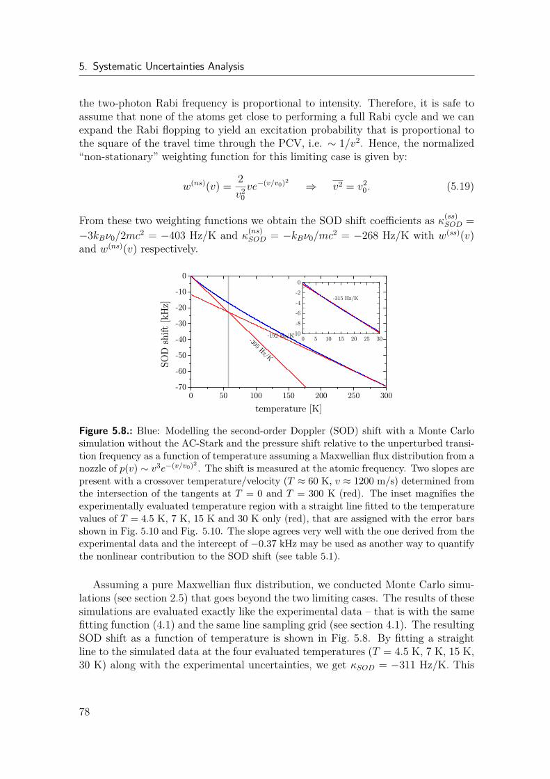
5. Systematic Uncertainties Analysis
the two-photon Rabi frequency is proportional to intensity. Therefore, it is safe toassume that none of the atoms get close to performing a full Rabi cycle and we canexpand the Rabi flopping to yield an excitation probability that is proportional tothe square of the travel time through the PCV, i.e. ∼ 1/v2. Hence, the normalized“non-stationary” weighting function for this limiting case is given by:
w(ns)(v) = 2v2
0ve−(v/v0)2 ⇒ v2 = v2
0. (5.19)
From these two weighting functions we obtain the SOD shift coefficients as κ(ss)SOD =
−3kBν0/2mc2 = −403 Hz/K and κ(ns)SOD = −kBν0/mc
2 = −268 Hz/K with w(ss)(v)and w(ns)(v) respectively.
Figure 5.8.: Blue: Modelling the second-order Doppler (SOD) shift with a Monte Carlosimulation without the AC-Stark and the pressure shift relative to the unperturbed transi-tion frequency as a function of temperature assuming a Maxwellian flux distribution from anozzle of p(v) ∼ v3e−(v/v0)2 . The shift is measured at the atomic frequency. Two slopes arepresent with a crossover temperature/velocity (T ≈ 60 K, v ≈ 1200 m/s) determined fromthe intersection of the tangents at T = 0 and T = 300 K (red). The inset magnifies theexperimentally evaluated temperature region with a straight line fitted to the temperaturevalues of T = 4.5 K, 7 K, 15 K and 30 K only (red), that are assigned with the error barsshown in Fig. 5.10 and Fig. 5.10. The slope agrees very well with the one derived from theexperimental data and the intercept of −0.37 kHz may be used as another way to quantifythe nonlinear contribution to the SOD shift (see table 5.1).
Assuming a pure Maxwellian flux distribution, we conducted Monte Carlo simu-lations (see section 2.5) that goes beyond the two limiting cases. The results of thesesimulations are evaluated exactly like the experimental data – that is with the samefitting function (4.1) and the same line sampling grid (see section 4.1). The resultingSOD shift as a function of temperature is shown in Fig. 5.8. By fitting a straightline to the simulated data at the four evaluated temperatures (T = 4.5 K, 7 K, 15 K,30 K) along with the experimental uncertainties, we get κSOD = −311 Hz/K. This
78
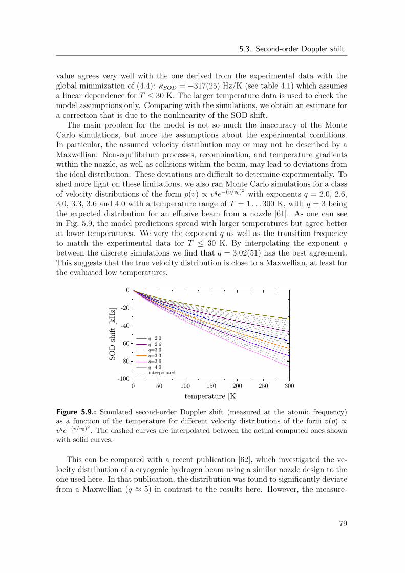
5.3. Second-order Doppler shift
value agrees very well with the one derived from the experimental data with theglobal minimization of (4.4): κSOD = −317(25) Hz/K (see table 4.1) which assumesa linear dependence for T ≤ 30 K. The larger temperature data is used to check themodel assumptions only. Comparing with the simulations, we obtain an estimate fora correction that is due to the nonlinearity of the SOD shift.
The main problem for the model is not so much the inaccuracy of the MonteCarlo simulations, but more the assumptions about the experimental conditions.In particular, the assumed velocity distribution may or may not be described by aMaxwellian. Non-equilibrium processes, recombination, and temperature gradientswithin the nozzle, as well as collisions within the beam, may lead to deviations fromthe ideal distribution. These deviations are difficult to determine experimentally. Toshed more light on these limitations, we also ran Monte Carlo simulations for a classof velocity distributions of the form p(v) ∝ vqe−(v/v0)2 with exponents q = 2.0, 2.6,3.0, 3.3, 3.6 and 4.0 with a temperature range of T = 1 . . . 300 K, with q = 3 beingthe expected distribution for an effusive beam from a nozzle [61]. As one can seein Fig. 5.9, the model predictions spread with larger temperatures but agree betterat lower temperatures. We vary the exponent q as well as the transition frequencyto match the experimental data for T ≤ 30 K. By interpolating the exponent qbetween the discrete simulations we find that q = 3.02(51) has the best agreement.This suggests that the true velocity distribution is close to a Maxwellian, at least forthe evaluated low temperatures.
Figure 5.9.: Simulated second-order Doppler shift (measured at the atomic frequency)as a function of the temperature for different velocity distributions of the form v(p) ∝vqe−(v/v0)2 . The dashed curves are interpolated between the actual computed ones shownwith solid curves.
This can be compared with a recent publication [62], which investigated the ve-locity distribution of a cryogenic hydrogen beam using a similar nozzle design to theone used here. In that publication, the distribution was found to significantly deviatefrom a Maxwellian (q ≈ 5) in contrast to the results here. However, the measure-
79
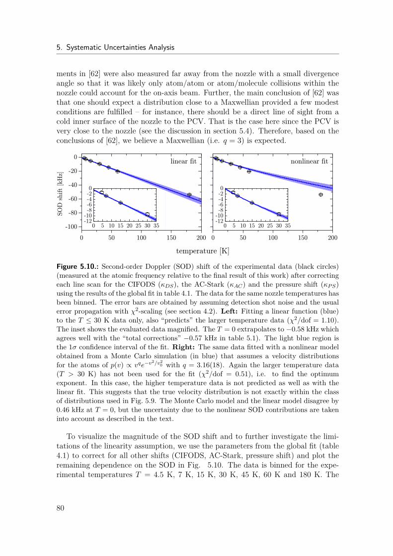
5. Systematic Uncertainties Analysis
ments in [62] were also measured far away from the nozzle with a small divergenceangle so that it was likely only atom/atom or atom/molecule collisions within thenozzle could account for the on-axis beam. Further, the main conclusion of [62] wasthat one should expect a distribution close to a Maxwellian provided a few modestconditions are fulfilled – for instance, there should be a direct line of sight from acold inner surface of the nozzle to the PCV. That is the case here since the PCV isvery close to the nozzle (see the discussion in section 5.4). Therefore, based on theconclusions of [62], we believe a Maxwellian (i.e. q = 3) is expected.
Figure 5.10.: Second-order Doppler (SOD) shift of the experimental data (black circles)(measured at the atomic frequency relative to the final result of this work) after correctingeach line scan for the CIFODS (κDS), the AC-Stark (κAC) and the pressure shift (κPS)using the results of the global fit in table 4.1. The data for the same nozzle temperatures hasbeen binned. The error bars are obtained by assuming detection shot noise and the usualerror propagation with χ2-scaling (see section 4.2). Left: Fitting a linear function (blue)to the T ≤ 30 K data only, also “predicts” the larger temperature data (χ2/dof = 1.10).The inset shows the evaluated data magnified. The T = 0 extrapolates to −0.58 kHz whichagrees well with the “total corrections” −0.57 kHz in table 5.1). The light blue region isthe 1σ confidence interval of the fit. Right: The same data fitted with a nonlinear modelobtained from a Monte Carlo simulation (in blue) that assumes a velocity distributionsfor the atoms of p(v) ∝ vqe−v
2/v20 with q = 3.16(18). Again the larger temperature data
(T > 30 K) has not been used for the fit (χ2/dof = 0.51), i.e. to find the optimumexponent. In this case, the higher temperature data is not predicted as well as with thelinear fit. This suggests that the true velocity distribution is not exactly within the classof distributions used in Fig. 5.9. The Monte Carlo model and the linear model disagree by0.46 kHz at T = 0, but the uncertainty due to the nonlinear SOD contributions are takeninto account as described in the text.
To visualize the magnitude of the SOD shift and to further investigate the limi-tations of the linearity assumption, we use the parameters from the global fit (table4.1) to correct for all other shifts (CIFODS, AC-Stark, pressure shift) and plot theremaining dependence on the SOD in Fig. 5.10. The data is binned for the expe-rimental temperatures T = 4.5 K, 7 K, 15 K, 30 K, 45 K, 60 K and 180 K. The
80
5.4. Pressure shift
larger temperatures (T > 30 K), that have not been used in the global minimization,are nevertheless corrected with the same parameters. The linear model fits the lowtemperature data very well and even describes the larger temperatures within theconfidence bands. In contrast, using the Monte Carlo simulations with q = 3.16(18)obtained by using the temperatures T ≤ 30 K does not “predict” the larger tempe-rature behaviour as well as the simple linear model. This reveals a limitation of themodel. As a consequence, we apply the linearity assumption but quadratically addthe full range of simulations, i.e. the difference between the q = 2 and q = 4 modelsto the experimental uncertainties σ1,i (but not to σ2,i and σ3,i; see section 4.4). Inthis way we also put more weight on the low temperature data, increase the errorbar for the less certain larger temperatures, and ignore the largest temperatures.The error bars shown in Fig. 5.10 are not enlarged in this way. At a temperature of7 K the SOD shift requires a correction of +2.2 kHz (+3.2 kHz for all data, see table5.1). We emphasize that we need to understand this correction only to within say10% in order to prevent it from contributing significantly to our final error budget.From the linear SOD extrapolation we get an uncertainty of 0.26 kHz as describedin section 5.12 and listed in the error budget shown in table 5.1.
5.4. Pressure shiftThe hydrogen atoms in the beam collide with other hydrogen atoms in the 1S and3S state as well as with hydrogen molecules that have not been dissociated or haverecombined inside the nozzle. All of them give rise to different collisional shifts (i.e.pressure shifts), and all can be taken as being proportional to the number of collisionsper second, which is in turn proportional to the density or flux of atoms/molecules. Inorder to extrapolate the pressure shift from intra-beam collisions to zero, we changedthe distance between the PCV center and the hydrogen nozzle by translating thenozzle along the laser beam. Two distances, d1 = 19.1 mm and d2 = 27.1 mm, havebeen used for the current data set. We assume the pressure shift is proportional tothe density of colliding atoms and undissociated molecules. The density of atomsand molecules from the beam is expected to reduce as the square of the distance fromthe source. We do not rely on this assumption, but instead calibrate the intra-beamdensity from the line amplitudes (see below).
As a consistency check, we have tried to locate the source point by extrapolatingthe observed line amplitudes. Atoms and molecules that escape the nozzle haveeither collided with other atoms or molecules inside the nozzle, or have emergedfrom the inner surface of the nozzle. Since the PCV is close to the nozzle, there is adirect line of sight to the inner wall of the back orifice. Unintentionally, the diameterof the back orifice was made 200 µm smaller than the front orifice (1.3 mm instead of1.5 mm) as we found out after the measurement, thereby increasing the visible innersurface. To better locate the source point and to get a good estimate of the local fluxof atoms within the beam, we mounted the fibers that detect the Doppler-broadened
81
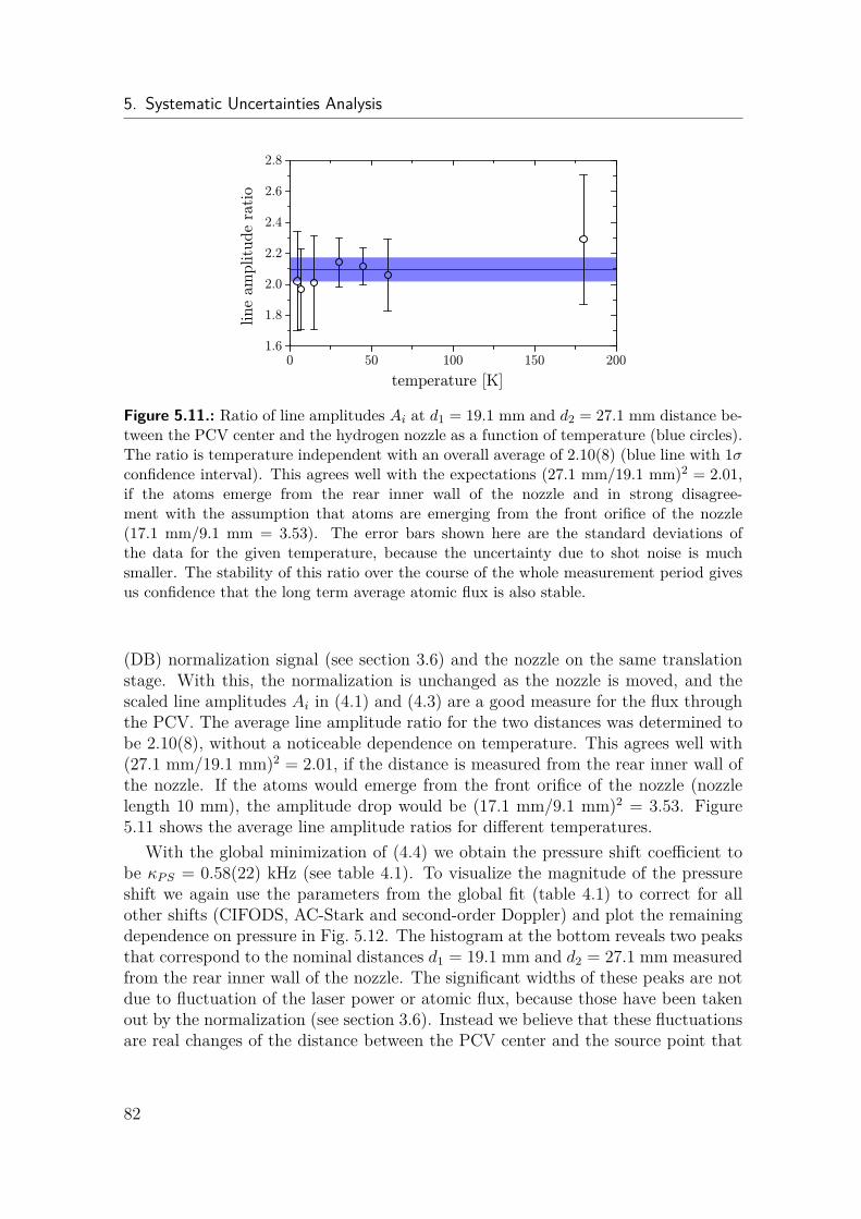
5. Systematic Uncertainties Analysis
Figure 5.11.: Ratio of line amplitudes Ai at d1 = 19.1 mm and d2 = 27.1 mm distance be-tween the PCV center and the hydrogen nozzle as a function of temperature (blue circles).The ratio is temperature independent with an overall average of 2.10(8) (blue line with 1σconfidence interval). This agrees well with the expectations (27.1 mm/19.1 mm)2 = 2.01,if the atoms emerge from the rear inner wall of the nozzle and in strong disagree-ment with the assumption that atoms are emerging from the front orifice of the nozzle(17.1 mm/9.1 mm = 3.53). The error bars shown here are the standard deviations ofthe data for the given temperature, because the uncertainty due to shot noise is muchsmaller. The stability of this ratio over the course of the whole measurement period givesus confidence that the long term average atomic flux is also stable.
(DB) normalization signal (see section 3.6) and the nozzle on the same translationstage. With this, the normalization is unchanged as the nozzle is moved, and thescaled line amplitudes Ai in (4.1) and (4.3) are a good measure for the flux throughthe PCV. The average line amplitude ratio for the two distances was determined tobe 2.10(8), without a noticeable dependence on temperature. This agrees well with(27.1 mm/19.1 mm)2 = 2.01, if the distance is measured from the rear inner wall ofthe nozzle. If the atoms would emerge from the front orifice of the nozzle (nozzlelength 10 mm), the amplitude drop would be (17.1 mm/9.1 mm)2 = 3.53. Figure5.11 shows the average line amplitude ratios for different temperatures.
With the global minimization of (4.4) we obtain the pressure shift coefficient tobe κPS = 0.58(22) kHz (see table 4.1). To visualize the magnitude of the pressureshift we again use the parameters from the global fit (table 4.1) to correct for allother shifts (CIFODS, AC-Stark and second-order Doppler) and plot the remainingdependence on pressure in Fig. 5.12. The histogram at the bottom reveals two peaksthat correspond to the nominal distances d1 = 19.1 mm and d2 = 27.1 mm measuredfrom the rear inner wall of the nozzle. The significant widths of these peaks are notdue to fluctuation of the laser power or atomic flux, because those have been takenout by the normalization (see section 3.6). Instead we believe that these fluctuationsare real changes of the distance between the PCV center and the source point that
82
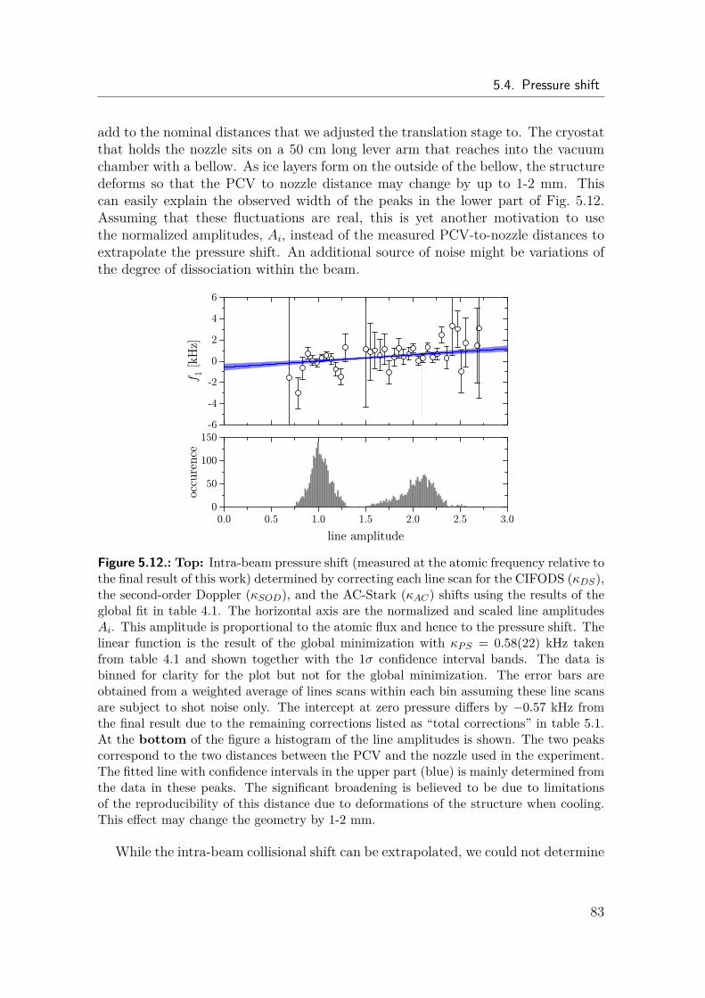
5.4. Pressure shift
add to the nominal distances that we adjusted the translation stage to. The cryostatthat holds the nozzle sits on a 50 cm long lever arm that reaches into the vacuumchamber with a bellow. As ice layers form on the outside of the bellow, the structuredeforms so that the PCV to nozzle distance may change by up to 1-2 mm. Thiscan easily explain the observed width of the peaks in the lower part of Fig. 5.12.Assuming that these fluctuations are real, this is yet another motivation to usethe normalized amplitudes, Ai, instead of the measured PCV-to-nozzle distances toextrapolate the pressure shift. An additional source of noise might be variations ofthe degree of dissociation within the beam.
Figure 5.12.: Top: Intra-beam pressure shift (measured at the atomic frequency relative tothe final result of this work) determined by correcting each line scan for the CIFODS (κDS),the second-order Doppler (κSOD), and the AC-Stark (κAC) shifts using the results of theglobal fit in table 4.1. The horizontal axis are the normalized and scaled line amplitudesAi. This amplitude is proportional to the atomic flux and hence to the pressure shift. Thelinear function is the result of the global minimization with κPS = 0.58(22) kHz takenfrom table 4.1 and shown together with the 1σ confidence interval bands. The data isbinned for clarity for the plot but not for the global minimization. The error bars areobtained from a weighted average of lines scans within each bin assuming these line scansare subject to shot noise only. The intercept at zero pressure differs by −0.57 kHz fromthe final result due to the remaining corrections listed as “total corrections” in table 5.1.At the bottom of the figure a histogram of the line amplitudes is shown. The two peakscorrespond to the two distances between the PCV and the nozzle used in the experiment.The fitted line with confidence intervals in the upper part (blue) is mainly determined fromthe data in these peaks. The significant broadening is believed to be due to limitationsof the reproducibility of this distance due to deformations of the structure when cooling.This effect may change the geometry by 1-2 mm.
While the intra-beam collisional shift can be extrapolated, we could not determine
83
5. Systematic Uncertainties Analysis
the collisional shift from the background gas experimentally. The pressure is mea-sured to be around 10−5 mbar with an ionization gauge placed in the central sectionof the vacuum chamber where the spectroscopy takes place. To estimate the back-ground pressure shift, we are using a simple theoretical model based on the so-calledimpact approximation [67], which assumes long-range interactions between collidingspecies. The long-range van-der-Waals interaction between two hydrogen atoms wastheoretically investigated in [68]. The interaction between hydrogen molecules andhydrogen atoms is more difficult to compute due to the complicated structure ofthe molecular levels. As an estimate, we assume that the van-der-Waals coefficienthas the same order of magnitude. The physical reason for this choice is that thefirst dipole-allowed transition from the ground state of a hydrogen molecule is about12.4 eV, which is close to the first dipole-allowed transition in atomic hydrogen of10.2 eV. This allows us to treat the background gas as atomic hydrogen only.
Most of the measurements in this work have been done at a temperature of 7 K,which is much smaller than the temperature of the background gas (≈ 300 K). Amodel for the collisional shift experienced by a slow atomic beam that is emerged ina gas of faster moving atoms has been developed in [69] and is described by:
δνPS = 1.293882π n ξ(6)
ω
(kBTBmB
)3/10
, (5.20)
where n is a number density of the particles of the background gas, and TB is thetemperature of the background gas with a particle mass of mB. The coefficientξ(6)ω = −4.325 × 10⁻¹⁷ rad m2(m/s)2/5 has been obtained in [69]. It is based onthe calculation of the van-der-Waals interaction coefficients derived in [68]. Withthese numbers we obtain an estimate of the background gas pressure shift of about−90 Hz. Since our assumptions here are rather crude, we choose not to correct forthis value but instead take its magnitude as an uncertainty (see table 5.1).
5.5. DC-Stark shiftThe DC-Stark shift can be a significant problem for precision spectroscopy if strayelectric fields are not properly compensated or shielded. In particular, at low tem-peratures a layer of frozen gases might build up at the surfaces of the nozzle. Freecharges from ionized hydrogen and other photoionizations due to the excitation lasercan build up on this layer and give rise to stray electric fields that can shift andbroaden the line. This problem is aggravated in our apparatus because the pulsecollision volume (PCV) is relatively close to the nozzle in order to obtain a largecount rate. This is a disadvantage compared to the more traditional continuous-wave excitation where the signal is generated far from non-conducting surfaces [7].However, our compensation and shielding can be more effective in a small volumesince, in practice, compensation works at one position in space only and otherwise
84
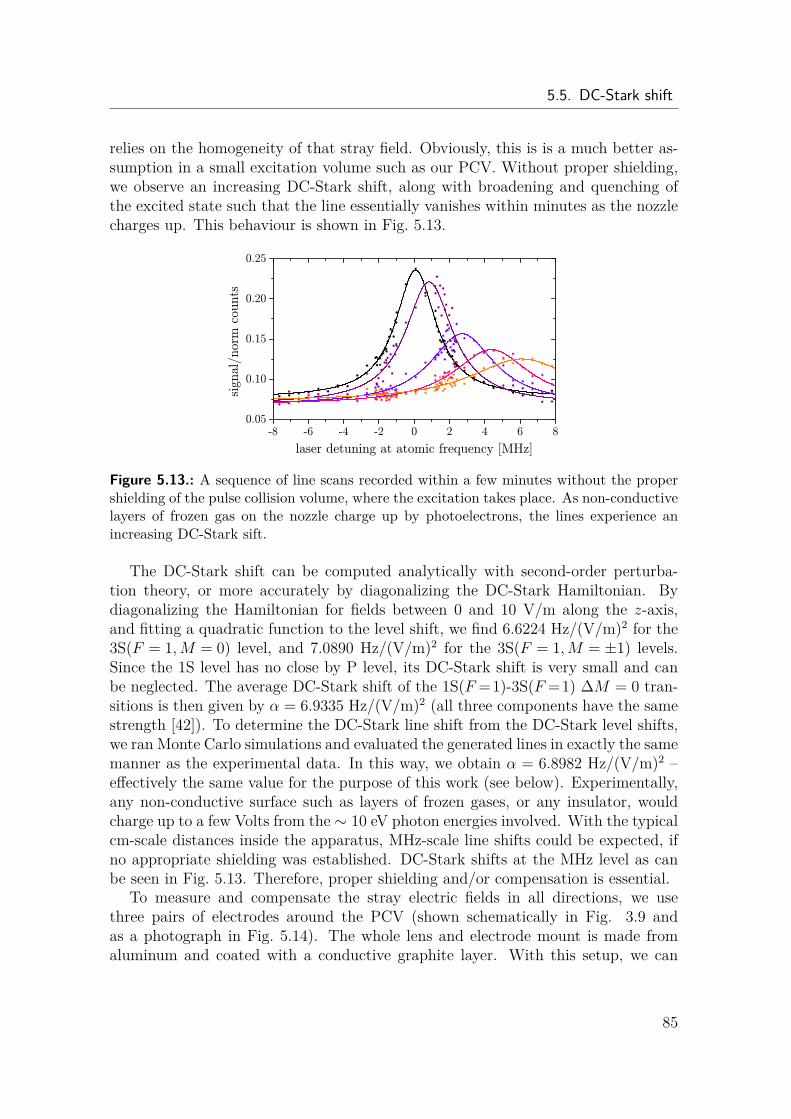
5.5. DC-Stark shift
relies on the homogeneity of that stray field. Obviously, this is is a much better as-sumption in a small excitation volume such as our PCV. Without proper shielding,we observe an increasing DC-Stark shift, along with broadening and quenching ofthe excited state such that the line essentially vanishes within minutes as the nozzlecharges up. This behaviour is shown in Fig. 5.13.
Figure 5.13.: A sequence of line scans recorded within a few minutes without the propershielding of the pulse collision volume, where the excitation takes place. As non-conductivelayers of frozen gas on the nozzle charge up by photoelectrons, the lines experience anincreasing DC-Stark sift.
The DC-Stark shift can be computed analytically with second-order perturba-tion theory, or more accurately by diagonalizing the DC-Stark Hamiltonian. Bydiagonalizing the Hamiltonian for fields between 0 and 10 V/m along the z-axis,and fitting a quadratic function to the level shift, we find 6.6224 Hz/(V/m)2 for the3S(F = 1,M = 0) level, and 7.0890 Hz/(V/m)2 for the 3S(F = 1,M = ±1) levels.Since the 1S level has no close by P level, its DC-Stark shift is very small and canbe neglected. The average DC-Stark shift of the 1S(F =1)-3S(F =1) ∆M = 0 tran-sitions is then given by α = 6.9335 Hz/(V/m)2 (all three components have the samestrength [42]). To determine the DC-Stark line shift from the DC-Stark level shifts,we ran Monte Carlo simulations and evaluated the generated lines in exactly the samemanner as the experimental data. In this way, we obtain α = 6.8982 Hz/(V/m)2 –effectively the same value for the purpose of this work (see below). Experimentally,any non-conductive surface such as layers of frozen gases, or any insulator, wouldcharge up to a few Volts from the ∼ 10 eV photon energies involved. With the typicalcm-scale distances inside the apparatus, MHz-scale line shifts could be expected, ifno appropriate shielding was established. DC-Stark shifts at the MHz level as canbe seen in Fig. 5.13. Therefore, proper shielding and/or compensation is essential.
To measure and compensate the stray electric fields in all directions, we usethree pairs of electrodes around the PCV (shown schematically in Fig. 3.9 andas a photograph in Fig. 5.14). The whole lens and electrode mount is made fromaluminum and coated with a conductive graphite layer. With this setup, we can
85
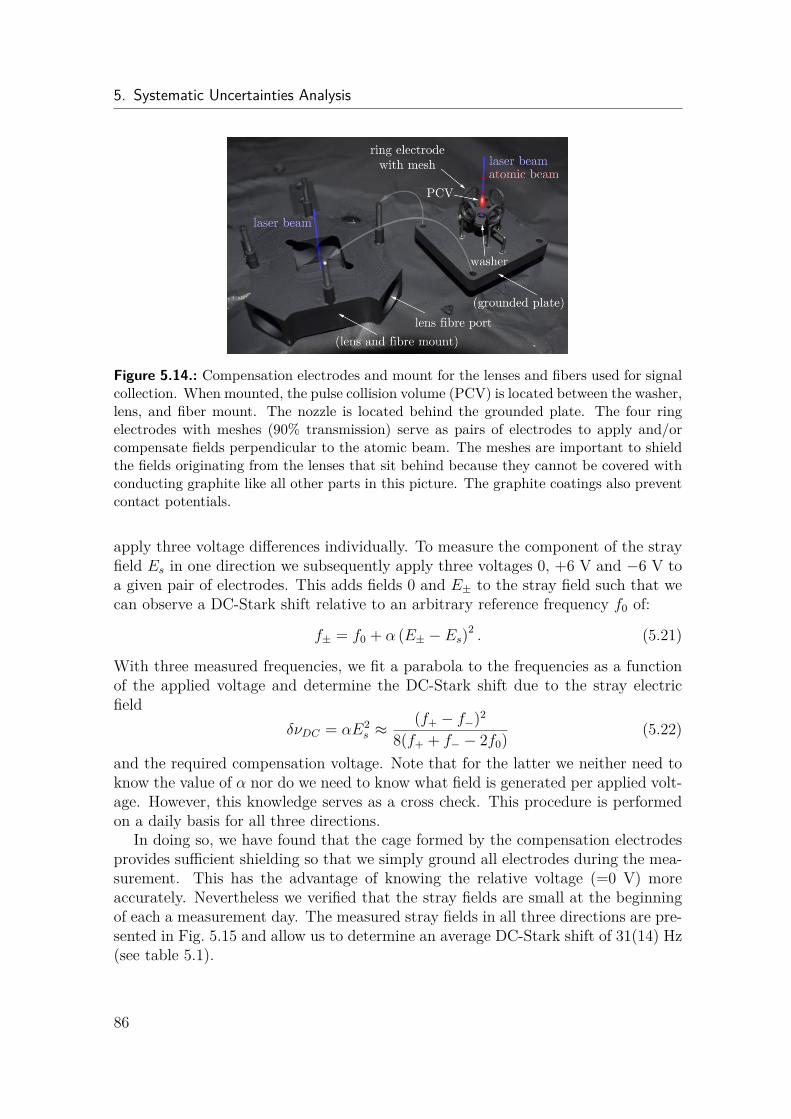
5. Systematic Uncertainties Analysis
Figure 5.14.: Compensation electrodes and mount for the lenses and fibers used for signalcollection. When mounted, the pulse collision volume (PCV) is located between the washer,lens, and fiber mount. The nozzle is located behind the grounded plate. The four ringelectrodes with meshes (90% transmission) serve as pairs of electrodes to apply and/orcompensate fields perpendicular to the atomic beam. The meshes are important to shieldthe fields originating from the lenses that sit behind because they cannot be covered withconducting graphite like all other parts in this picture. The graphite coatings also preventcontact potentials.
apply three voltage differences individually. To measure the component of the strayfield Es in one direction we subsequently apply three voltages 0, +6 V and −6 V toa given pair of electrodes. This adds fields 0 and E± to the stray field such that wecan observe a DC-Stark shift relative to an arbitrary reference frequency f0 of:
f± = f0 + α (E± − Es)2 . (5.21)
With three measured frequencies, we fit a parabola to the frequencies as a functionof the applied voltage and determine the DC-Stark shift due to the stray electricfield
δνDC = αE2s ≈
(f+ − f−)2
8(f+ + f− − 2f0) (5.22)
and the required compensation voltage. Note that for the latter we neither need toknow the value of α nor do we need to know what field is generated per applied volt-age. However, this knowledge serves as a cross check. This procedure is performedon a daily basis for all three directions.
In doing so, we have found that the cage formed by the compensation electrodesprovides sufficient shielding so that we simply ground all electrodes during the mea-surement. This has the advantage of knowing the relative voltage (=0 V) moreaccurately. Nevertheless we verified that the stray fields are small at the beginningof each a measurement day. The measured stray fields in all three directions are pre-sented in Fig. 5.15 and allow us to determine an average DC-Stark shift of 31(14) Hz(see table 5.1).
86
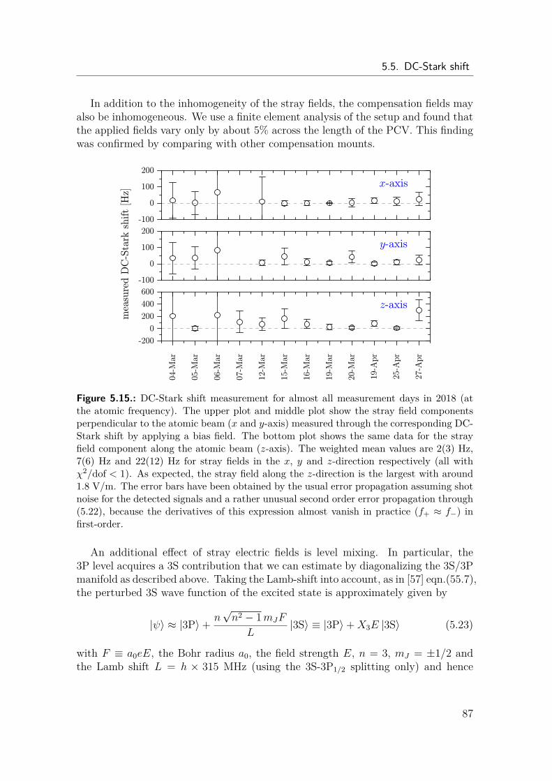
5.5. DC-Stark shift
In addition to the inhomogeneity of the stray fields, the compensation fields mayalso be inhomogeneous. We use a finite element analysis of the setup and found thatthe applied fields vary only by about 5% across the length of the PCV. This findingwas confirmed by comparing with other compensation mounts.
Figure 5.15.: DC-Stark shift measurement for almost all measurement days in 2018 (atthe atomic frequency). The upper plot and middle plot show the stray field componentsperpendicular to the atomic beam (x and y-axis) measured through the corresponding DC-Stark shift by applying a bias field. The bottom plot shows the same data for the strayfield component along the atomic beam (z-axis). The weighted mean values are 2(3) Hz,7(6) Hz and 22(12) Hz for stray fields in the x, y and z-direction respectively (all withχ2/dof < 1). As expected, the stray field along the z-direction is the largest with around1.8 V/m. The error bars have been obtained by the usual error propagation assuming shotnoise for the detected signals and a rather unusual second order error propagation through(5.22), because the derivatives of this expression almost vanish in practice (f+ ≈ f−) infirst-order.
An additional effect of stray electric fields is level mixing. In particular, the3P level acquires a 3S contribution that we can estimate by diagonalizing the 3S/3Pmanifold as described above. Taking the Lamb-shift into account, as in [57] eqn.(55.7),the perturbed 3S wave function of the excited state is approximately given by
|ψ〉 ≈ |3P〉+ n√n2 − 1mJF
L|3S〉 ≡ |3P〉+X3E |3S〉 (5.23)
with F ≡ a0eE, the Bohr radius a0, the field strength E, n = 3, mJ = ±1/2 andthe Lamb shift L = h × 315 MHz (using the 3S-3P1/2 splitting only) and hence
87
5. Systematic Uncertainties Analysis
X3 = 1.7 × 10⁻⁴ (m/V). This mixing allows for 1S-3P excitation with two-photonsand a Rabi frequency of Ω1S-3P = X3E Ω1S-3S = 3.4 × 10⁻⁴ Ω1S-3S. The last numberis obtained with the maximum field of 1.8 V/m detected in the experiment (seeFig. 5.15). The relative line strength of the 1S-3P line is given by the square ofthe ratio of the Rabi-frequencies and hence the extra line has a relative strength of1.2×10−7. It is folded into the spectrum with the frequency comb and has hyperfinecomponents and a line width of 29.5 MHz [57]. To get an upper limit of the linepulling effect, we generate artificial line scan data by adding the weak 1S-3P line tothe fully allowed lines with various detunings and fit the result in the same manneras the experimental data. The maximum line pulling obtained in this way is 4 mHz.
Not only does the 3P state acquire a small 3S admixture, the 3S state also obtainsa small 3P component through an external DC field, which leads to an additionalline broadening. With the same formalism we obtain for the 3S state:
|ψ〉 ≈ |3S〉+ n√n2 − 1mJF
L|3P〉 ≡ |3S〉 −X3E |3P〉 (5.24)
In addition to the 3S→2P decay matrix element, we obtain an additional decay paththrough the 3P→2S channel. Since the inverse lifetime τ3S is proportional to thematrix elements squared, we obtain:
1τ3S
= 1τ3S-2P
+ X23E
2
τ3P-2S= 1
158.37 ns + X23E
2
5.4 ns . (5.25)
With E = 1.8 V/m the line width increases by X23E
2/(2π×5.4 ns) = 3.4 Hz only. Wecan also use the two-photon optical Bloch equations (see section 2.5) to verify thesesmall effects. Numerically we obtain a line broadening of 0.72 Hz/(V/m)2, which iscomparable to the analytic treatment given above. With the full level scheme wecould also verify the line pulling due to the 3S-3P excitation. However, the numericalsimulation does not allow us to separate the discussed line pulling from the directDC-Stark shift.
5.6. Zeeman shiftThe Zeeman shift of a hydrogenic S(F,M) state with a nuclear spin 1/2 is obtainedin first approximation with the Breit-Rabi formula
− A
4 +MgNµNB ±A
2√
1 + 2Mx(A) + x(A)2, (5.26)
where the “+” sign belongs to the F = 1 total angular momentum and the “−” signto F = 0. Further, x(A) ≡ (gJµB − gNµN)B/A, the external stray magnetic field isgiven by B, the electronic and nuclear g-factors are given by gJ and gN , the Bohrand nuclear magneton are given by µB and µN = µBme/mp, and the hyperfine
88
5.6. Zeeman shift
splitting is given by A. The latter is very well measured for the 1S state, A1S =1 420 405 751.766 7(10) Hz [78] and extrapolated to the excited states with A3S =52 609 473.2(3) Hz [10]. With the circular σ+/σ− polarization, all three componentsof the 1S(F = 1,M) → 3S(F = 1,M) compatible with the ∆M = 0 selection ruleare excited with the same strength [42].
With (5.26), we obtain a Zeeman shift of the F = 1,M = ±1 levels:
A
4 ±(gJµB + 1
2gNµN)B. (5.27)
The Landé g-factors gJ = 2, and the nuclear (proton) g-factor gN = 2.7928473508(85) [4]are identical for the 1S and the 3S level so that the Zeeman shift is cancelled exactlyfor these components within this level of approximation. For the F = 1,M = 0 com-ponent, we can expand the level shift (5.26), and find for the shift of the transitionfrequency:
δνM=0Zee ≈
A3S
4 x(A3S)2 − A1S
4 x(A1S)2 = 35.802 kHzGauss2 B2. (5.28)
In our setup we compensate the stray magnetic field in all three directions within thePCV using 3 pairs of Helmholtz coils. The residual fields have been measured severaltimes during the measurement campaign and were found to be 14(15) mG. Thanksto the quadratic dependence, the corresponding Zeeman shift is only 7.0(8.0) Hz.
One may ask if possible imperfections that are not taken into account above –for instance polarization imperfections – increase this shift. However, the ∆M = 0selection rule holds for any polarization [42]. The physical reason is that the two-photon operator does not act on spins, and there is no orbital angular momentumexchanged in an S-S transition.
In addition, relativistic corrections requires one to multiply the g-factors in (5.27)with a state dependent factor, which is given in first-order for the electron spin as(see [57] eqn.(47.4)):
1− α2
3n2 (5.29)
resulting in a linear Zeeman shift of the F = 1,M = ±1 transitions of:
δνM=±1Zee = ± 8
27 gJα2µBB = ± 44Hz
Gauss B. (5.30)
Note that the anomalous g-factor part cancels and only the state dependent part isrelevant for the Zeeman shift. Higher order terms and the corresponding correctionto the nuclear movement are neglected here. Effectively this very small shift turnsinto a mere line broadening if both components F = 1,M = +1 and F = 1,M = −1occur with equal strength.
Lastly, the Breit-Rabi formula (5.26) is obtained by dialogizing the four-levelHFS Hamiltonian, ignoring all other states. For completeness we have also included
89
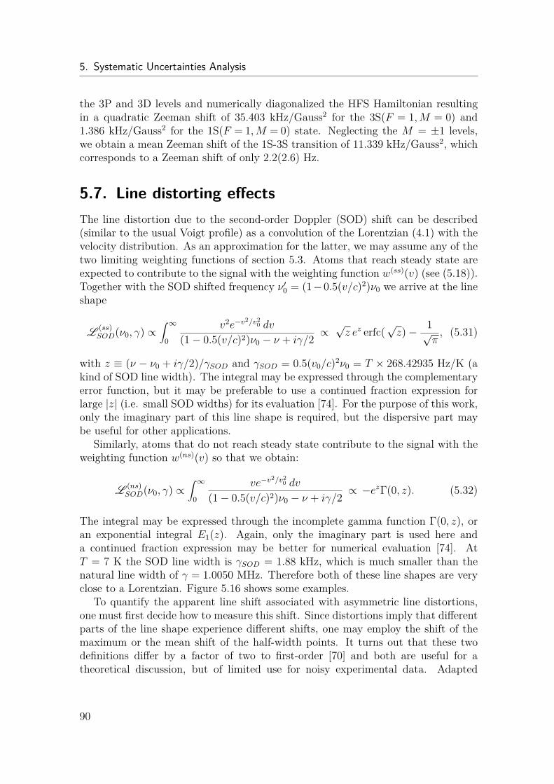
5. Systematic Uncertainties Analysis
the 3P and 3D levels and numerically diagonalized the HFS Hamiltonian resultingin a quadratic Zeeman shift of 35.403 kHz/Gauss2 for the 3S(F = 1,M = 0) and1.386 kHz/Gauss2 for the 1S(F = 1,M = 0) state. Neglecting the M = ±1 levels,we obtain a mean Zeeman shift of the 1S-3S transition of 11.339 kHz/Gauss2, whichcorresponds to a Zeeman shift of only 2.2(2.6) Hz.
5.7. Line distorting effectsThe line distortion due to the second-order Doppler (SOD) shift can be described(similar to the usual Voigt profile) as a convolution of the Lorentzian (4.1) with thevelocity distribution. As an approximation for the latter, we may assume any of thetwo limiting weighting functions of section 5.3. Atoms that reach steady state areexpected to contribute to the signal with the weighting function w(ss)(v) (see (5.18)).Together with the SOD shifted frequency ν ′0 = (1−0.5(v/c)2)ν0 we arrive at the lineshape
L (ss)SOD(ν0, γ) ∝
∫ ∞0
v2e−v2/v2
0 dv
(1− 0.5(v/c)2)ν0 − ν + iγ/2 ∝√z ez erfc(
√z)− 1√
π, (5.31)
with z ≡ (ν − ν0 + iγ/2)/γSOD and γSOD = 0.5(v0/c)2ν0 = T × 268.42935 Hz/K (akind of SOD line width). The integral may be expressed through the complementaryerror function, but it may be preferable to use a continued fraction expression forlarge |z| (i.e. small SOD widths) for its evaluation [74]. For the purpose of this work,only the imaginary part of this line shape is required, but the dispersive part maybe useful for other applications.
Similarly, atoms that do not reach steady state contribute to the signal with theweighting function w(ns)(v) so that we obtain:
L (ns)SOD(ν0, γ) ∝
∫ ∞0
ve−v2/v2
0 dv
(1− 0.5(v/c)2)ν0 − ν + iγ/2 ∝ −ezΓ(0, z). (5.32)
The integral may be expressed through the incomplete gamma function Γ(0, z), oran exponential integral E1(z). Again, only the imaginary part is used here anda continued fraction expression may be better for numerical evaluation [74]. AtT = 7 K the SOD line width is γSOD = 1.88 kHz, which is much smaller than thenatural line width of γ = 1.0050 MHz. Therefore both of these line shapes are veryclose to a Lorentzian. Figure 5.16 shows some examples.
To quantify the apparent line shift associated with asymmetric line distortions,one must first decide how to measure this shift. Since distortions imply that differentparts of the line shape experience different shifts, one may employ the shift of themaximum or the mean shift of the half-width points. It turns out that these twodefinitions differ by a factor of two to first-order [70] and both are useful for atheoretical discussion, but of limited use for noisy experimental data. Adapted
90
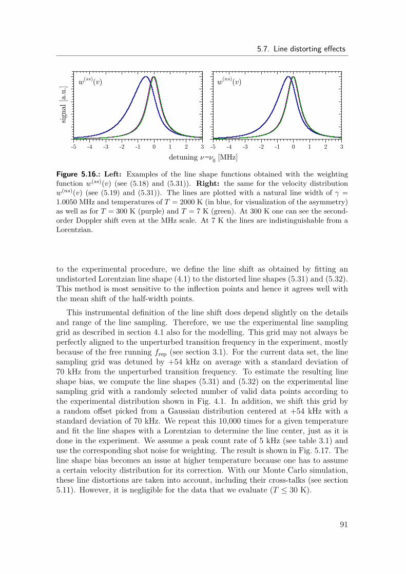
5.7. Line distorting effects
−
Figure 5.16.: Left: Examples of the line shape functions obtained with the weightingfunction w(ss)(v) (see (5.18) and (5.31)). Right: the same for the velocity distributionw(ns)(v) (see (5.19) and (5.31)). The lines are plotted with a natural line width of γ =1.0050 MHz and temperatures of T = 2000 K (in blue, for visualization of the asymmetry)as well as for T = 300 K (purple) and T = 7 K (green). At 300 K one can see the second-order Doppler shift even at the MHz scale. At 7 K the lines are indistinguishable from aLorentzian.
to the experimental procedure, we define the line shift as obtained by fitting anundistorted Lorentzian line shape (4.1) to the distorted line shapes (5.31) and (5.32).This method is most sensitive to the inflection points and hence it agrees well withthe mean shift of the half-width points.
This instrumental definition of the line shift does depend slightly on the detailsand range of the line sampling. Therefore, we use the experimental line samplinggrid as described in section 4.1 also for the modelling. This grid may not always beperfectly aligned to the unperturbed transition frequency in the experiment, mostlybecause of the free running frep (see section 3.1). For the current data set, the linesampling grid was detuned by +54 kHz on average with a standard deviation of70 kHz from the unperturbed transition frequency. To estimate the resulting lineshape bias, we compute the line shapes (5.31) and (5.32) on the experimental linesampling grid with a randomly selected number of valid data points according tothe experimental distribution shown in Fig. 4.1. In addition, we shift this grid bya random offset picked from a Gaussian distribution centered at +54 kHz with astandard deviation of 70 kHz. We repeat this 10,000 times for a given temperatureand fit the line shapes with a Lorentzian to determine the line center, just as it isdone in the experiment. We assume a peak count rate of 5 kHz (see table 3.1) anduse the corresponding shot noise for weighting. The result is shown in Fig. 5.17. Theline shape bias becomes an issue at higher temperature because one has to assumea certain velocity distribution for its correction. With our Monte Carlo simulation,these line distortions are taken into account, including their cross-talks (see section5.11). However, it is negligible for the data that we evaluate (T ≤ 30 K).
91
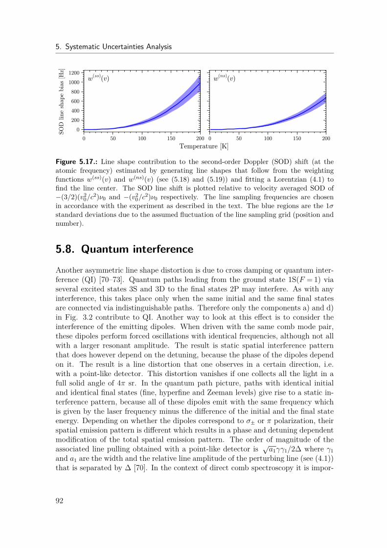
5. Systematic Uncertainties Analysis
Figure 5.17.: Line shape contribution to the second-order Doppler (SOD) shift (at theatomic frequency) estimated by generating line shapes that follow from the weightingfunctions w(ss)(v) and w(ns)(v) (see (5.18) and (5.19)) and fitting a Lorentzian (4.1) tofind the line center. The SOD line shift is plotted relative to velocity averaged SOD of−(3/2)(v2
0/c2)ν0 and −(v2
0/c2)ν0 respectively. The line sampling frequencies are chosen
in accordance with the experiment as described in the text. The blue regions are the 1σstandard deviations due to the assumed fluctuation of the line sampling grid (position andnumber).
5.8. Quantum interference
Another asymmetric line shape distortion is due to cross damping or quantum inter-ference (QI) [70–73]. Quantum paths leading from the ground state 1S(F = 1) viaseveral excited states 3S and 3D to the final states 2P may interfere. As with anyinterference, this takes place only when the same initial and the same final statesare connected via indistinguishable paths. Therefore only the components a) and d)in Fig. 3.2 contribute to QI. Another way to look at this effect is to consider theinterference of the emitting dipoles. When driven with the same comb mode pair,these dipoles perform forced oscillations with identical frequencies, although not allwith a larger resonant amplitude. The result is static spatial interference patternthat does however depend on the detuning, because the phase of the dipoles dependon it. The result is a line distortion that one observes in a certain direction, i.e.with a point-like detector. This distortion vanishes if one collects all the light in afull solid angle of 4π sr. In the quantum path picture, paths with identical initialand identical final states (fine, hyperfine and Zeeman levels) give rise to a static in-terference pattern, because all of these dipoles emit with the same frequency whichis given by the laser frequency minus the difference of the initial and the final stateenergy. Depending on whether the dipoles correspond to σ± or π polarization, theirspatial emission pattern is different which results in a phase and detuning dependentmodification of the total spatial emission pattern. The order of magnitude of theassociated line pulling obtained with a point-like detector is √a1γγ1/2∆ where γ1and a1 are the width and the relative line amplitude of the perturbing line (see (4.1))that is separated by ∆ [70]. In the context of direct comb spectroscopy it is impor-
92
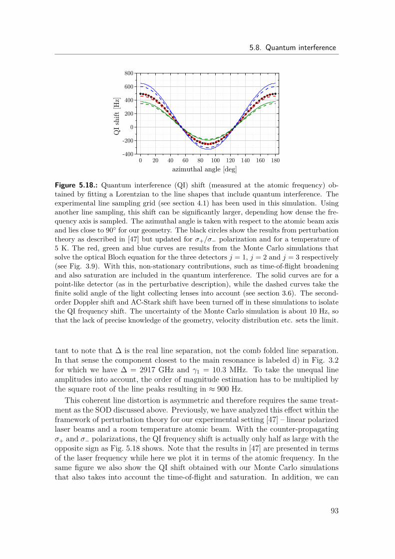
5.8. Quantum interference
Figure 5.18.: Quantum interference (QI) shift (measured at the atomic frequency) ob-tained by fitting a Lorentzian to the line shapes that include quantum interference. Theexperimental line sampling grid (see section 4.1) has been used in this simulation. Usinganother line sampling, this shift can be significantly larger, depending how dense the fre-quency axis is sampled. The azimuthal angle is taken with respect to the atomic beam axisand lies close to 90 for our geometry. The black circles show the results from perturbationtheory as described in [47] but updated for σ+/σ− polarization and for a temperature of5 K. The red, green and blue curves are results from the Monte Carlo simulations thatsolve the optical Bloch equation for the three detectors j = 1, j = 2 and j = 3 respectively(see Fig. 3.9). With this, non-stationary contributions, such as time-of-flight broadeningand also saturation are included in the quantum interference. The solid curves are for apoint-like detector (as in the perturbative description), while the dashed curves take thefinite solid angle of the light collecting lenses into account (see section 3.6). The second-order Doppler shift and AC-Stark shift have been turned off in these simulations to isolatethe QI frequency shift. The uncertainty of the Monte Carlo simulation is about 10 Hz, sothat the lack of precise knowledge of the geometry, velocity distribution etc. sets the limit.
tant to note that ∆ is the real line separation, not the comb folded line separation.In that sense the component closest to the main resonance is labeled d) in Fig. 3.2for which we have ∆ = 2917 GHz and γ1 = 10.3 MHz. To take the unequal lineamplitudes into account, the order of magnitude estimation has to be multiplied bythe square root of the line peaks resulting in ≈ 900 Hz.
This coherent line distortion is asymmetric and therefore requires the same treat-ment as the SOD discussed above. Previously, we have analyzed this effect within theframework of perturbation theory for our experimental setting [47] – linear polarizedlaser beams and a room temperature atomic beam. With the counter-propagatingσ+ and σ− polarizations, the QI frequency shift is actually only half as large with theopposite sign as Fig. 5.18 shows. Note that the results in [47] are presented in termsof the laser frequency while here we plot it in terms of the atomic frequency. In thesame figure we also show the QI shift obtained with our Monte Carlo simulationsthat also takes into account the time-of-flight and saturation. In addition, we can
93
5. Systematic Uncertainties Analysis
include the solid angle of the NA = 0.68 lenses that reduces this effect further. Evenwithout this reduction, the quantum interference frequency shift is small but we stillcorrect our final result by adding 0.25 kHz.
Additional asymmetric line distortions arise from time-of-flight and power broa-dening. These are small compared to the natural line width as the typical line scanin Fig. 4.2d shows. In fact, the lines recorded at low temperatures, with low laserpowers, and the down stream detector (j = 2) have line widths that are statisticallyindistinguishable from the natural line width. Moreover, these broadenings are sym-metric and hence do not produce an additional line shape contribution to the shiftdiscussed above.
5.9. Incoherent line pullingWe define incoherent line pulling as effects where the center of the line no longercoincides with the transition energy because of a sloping baseline caused by the pre-sence of other lines. In contrast to the previous section, we now discuss the situationswhere there is no static interference between these lines, so that the sloping baselineis the only pulling mechanism [70]. One could eliminate this effect by accountingfor the other components with an appropriate fitting function. For simplicity, weare fitting a single Lorentzian only (see section 4.2) and, as in the previous section,quantify the line pulling by employing an instrumental definition obtained by thefitting result. The incoherent line pulling is, in general, significantly smaller thanthe coherent line pulling through quantum interference [70].
5.9.1. Other line componentsAs seen in Fig. 3.2, other fine and hyperfine components are folded into the observedspectrum because of the comb excitation. The ps-comb has a spectral envelope thatis about 150 GHz wide and therefore covers all components of the n = 1 → n = 3transition (see Fig. 3.3). We have fine tuned the repetition rate in order to isolate themain component of interest (see section 3.2). Nevertheless, we have to investigatethe remaining line pulling. The different components that appear in the wrappedspectrum are excited with different comb pairs. This means their spatial interferencepattern is not static but beats at multiples of the repetition rate and the quantuminterference effect averages out during the 1 sec gate time of our detectors. Theresulting line pulling can be easily determined by modeling a spectrum as is shownin Fig. 3.2 consisting of 6 Lorentzians (with appropriate amplitude and widths) andthen fitting a single Lorentzian only (within the spectral range and with the linesampling used in the experiment). In this way, we obtain a negligible line pulling of−48.5 Hz, which justifies the use of a single Lorentzian for a simplified data analysis.
Another source of perturbing peaks in the spectrum are the imperfectly suppressedmodes of the laser. As detailed in section 3.2, the doubling cavities are operated
94
5.9. Incoherent line pulling
at twice the lasers repetition rate and hence also double the mode spacing from78.8 MHz to 157.6 MHz. As shown in section 3.3, the suppression of the 78.8 MHzspaced modes relative to 157.6 MHz modes is given by T 4, where T = 30% is thepower transmission of the input couplers of both of the doubling cavities. The 205 nmenhancement cavity is also operated at twice the laser repetition rate, even thoughwe effectively have four times the repetition rate for the Doppler-free excitation bycirculating two pulses simultaneously in this cavity. Assuming the 157.6 MHz spacedresonant modes are impedance-matched, they are power enhanced by 1/T1 whereasthe off-resonant 78.8 MHz spaced modes are further suppressed with the inversefactor. Here, T1 = 6.2% is the input coupler transmission of the 205 nm enhancementcavity. In total the unwanted modes are suppressed by m = T 4T 2
1 = 3.1 × 10⁻⁵, sothat we actually do not see them in the experimental data. Nevertheless we need toestimate their possible line pulling effect. We do this by solving the optical Blochequations of the full level scheme (see section 2.5) by assuming a superimposedcomb with a 78.8 MHz mode spacing that is suppressed by the above factor m.Analyzing this data exactly as the experimental data, we obtain a line pulling ofroughly δν = 4 kHz×m = 0.12 Hz, which can be safely ignored.
If the exciting frequency comb would have residual modes with a quarter integermode number, i.e. with a 78.8 MHz spacing, we can determine where the foldedline components a), b), c), d) and e) from Fig. 3.2 would reappear in the spec-trum. With the quarter integer mode numbers of +12.75, +13.75, +17.25, +9.25and +4.25 they are expected at a detuning from the main resonance of −18.7 MHz,+4.7 MHz, −18.3 MHz, +1.1 MHz and +28.2 MHz respectively. Unlike the extraline components discussed below, some of these detunings are too small to limit theline pulling just with the large line separation. One might find a limit by investi-gating the residuals in Fig. 4.5, but the amplitude limit presented above provides atighter limit in this case.
As explained in section 3.2, the propagation direction of the colliding pulses andtheir polarizations alternate. In the ideal case a σ+ polarized pulse from the left anda σ− polarized pulse from the right alternates with a σ− polarized pulse from theleft and a σ+ polarized pulse from the right. The electric field vectors add, forminga helix of a linear polarized standing field within the PCV whose position alternatesbetween collisions. In contrast, the Doppler free two-photon Rabi frequency (5.2)is obtained as the product of the counter-propagating fields. Therefore the Rabifrequency is not necessarily alternating, even if the electric field vector is. To see thatthis is indeed the case, independent of polarization, we write the counter-propagatingpulses as ~E+ = ~e+A(t − z/c) cos(ωct − kz − ϕ/2) and ~E− = ~e−A(t + z/c) cos(ωct +kz + ϕ/2) with z = 0 being center of the enhancement cavity, t = 0 the time of thefirst pulse collision, ~e± the polarizations, A(t) the pulse envelope and ϕ a possiblephase shift of the carrier frequency ωc. After one round trip time T , the propagationdirection is exchanged (z → −z) and the pulses are delayed: ~E+ = ~e−A(t + T +z/c) cos(ωc(t+ T ) + k(z− cT )−ϕ/2) = ~e−A(t+ z/c) cos(ωct+ kz−ϕ/2) and ~E− =
95
5. Systematic Uncertainties Analysis
~e+A(t+T −z/c) cos(ωc(t+T )−k(z+cT )+ϕ/2) = ~e+A(t+z/c) cos(ωct−kz+ϕ/2),where we assumed that the pulse envelopes are the same and periodic with T . Withinthe rotating wave approximation (for two-photon transitions) we keep only terms inthe product of the fields that oscillate with 2ωc. This means that kz-term drops outas it should (Doppler-free) and so does the ϕ-term. More important to the discussionhere is that the Rabi frequency is the same for the first pulse and after one roundtrip. Hence, within the rotating wave approximation, this mechanism does not leadto the emergence of a 157.6 MHz comb spacing in the recorded spectrum.
The discussion of the last paragraph assumes that the timing of the pulses issuch that they always meet at z = 0. However, the delay stage that is used togenerate the counter-propagating pulses may not be perfectly adjusted. As a resultone of the pulses is advanced and the other delayed by say δt which leads to a factorA(t − δt/2 − z/c)A(t + δt/2 + z/c) in the above Rabi frequency for the first pulsecollision. After one round trip the propagation direction is flipped and the pulse isdelayed such that the product of the envelopes becomes A(t−δt/2+(z−cT )/c)A(t+δt/2 − (z + cT )/c) = A(t − δt/2 + z/c)A(t + δt/2 − z/c), where we assumed againthat each pulse train is periodic. This means that the position of the PCV alternatesbetween z = ±c δt/2, i.e. by ∆z = c δt between subsequent pulse collision events. Asa consequence, atoms at a fixed position other than z = 0 experience an amplitudemodulated Rabi frequency at 157.6 MHz. We measure and set an upper limit onthe timing error of |c δt| < 40 µm as described in section 3.2. Then we model thiseffect by solving the optical Bloch equations of the full level scheme and analysethe generated data exactly like the real experimental data. In this way, we find afrequency pulling of δν = −0.0019 (Hz/µm2) ×(c δt)2 = −3.0 Hz, which can besafely ignored.
In addition we can also limit the line pulling 157.6 MHz comb component thatemerges through any mechanism with the experimental data. The folded line com-ponents a), b), c), d) and e) from Fig. 3.2 reappear with half integer mode numberoff-sets of +12.5, +13.5, +17.5, +9.5 and +4.5 at a detuning from the main resonanceof +60.1 MHz, +83.5 MHz, −97.1 MHz, −77.1 MHz and +50.6 MHz respectively.Hence, these additional line components, if they exist, are separated from the mainresonance by a detuning comparable to the other fine and hyperfine componentsdiscussed above. With their amplitude significantly lower, the resulting line pullingis also significantly lower and therefore negligible.
5.9.2. Forbidden ∆F = 1 componentsAnother possible source of incoherent line pulling may be due to the forbidden∆F = 1 hyperfine components (see level scheme in Fig. 3.2). Since no orbitalangular momentum is involved in the 1S-3S transition, the electron spin must fliprelative to the nuclear spin for a ∆F , 0 component. This is not possible with theelectric dipole operator that drives the two-photon transition [42]. Therefore thesecomponents are forbidden for any laser polarization such that we do not have to
96
5.9. Incoherent line pulling
discuss polarization imperfections in this context. However, higher order transitionamplitudes or perturbations by stray fields allow these components to some extent.
The location of these extra components within the spectrum are determined bythe very well known 1S and 3S hyperfine splittings and the mode spacing of ourfrequency comb. The 1S(F = 1) → 3S(F = 0) component appears at a detuning of−52.609 473 MHz [10], which is the excited state hyperfine splitting A3S, while the1S(F =0)→ 3S(F =0) component appears at a detuning of +2.005 752 MHz, whichis the ground state hyperfine splitting [78] A1S minus 4.5 times the mode spacingof the comb. Both forbidden components are closer to the main resonance than theallowed components (see Fig. 3.2). To estimate the resulting line pulling we ignorethe allowed components and again generate artificial data that contains one of theforbidden components with a line amplitude ratio r and fit a single Lorentzian. Indoing so (using the experimental line sampling), we find δν = 40 kHz × r for the1S(F =0)→ 3S(F =1) component and δν = −1.8 Hz×r for the 1S(F =1)→ 3S(F =0), linear in the relative amplitude r with very good approximation. The latter linepulling can be neglected given the observation that r 1, while the former requiresa more careful estimation of r. There are several conceivable mechanisms that mayallow this forbidden transition:
1. Only two-photon transitions are resonant and can give rise to a line in closeproximity with the main line. This might be combinations of the electricE1 and the magnetic M1 dipole or higher multipole operators. Relativisticcorrections to the matrix elements and levels might also be considered to allowthe forbidden transition. However, it follows from the Furry theorem that alltwo-photon excitations of the forbidden line without external perturbations areexcluded [60]. One way to read this theorem is that an odd number of photonscannot be converted to an even one without changing a state of something else(the atom). The two-photon excitation 1S(F =0)→ 3S(F =1) of any type andsubsequent single-photon decay via 3S(F = 1) → 1S(F = 0), that is certainlyallowed, would represent such a process. Hence, we can restrict the discussionhere to the role of external fields.
2. A stray electric field E mixes the 3P levels to the 3S levels and allows the1S(F = 0) → 3S(F = 1) transition. As derived in section 5.5, this admixtureleads to a Rabi frequency of Ω1S-3P = X3E Ω1S-3S = 3.4×10⁻⁴ Ω1S-3S. Again, theline amplitude ratio is given by the square of the ratio of the Rabi frequencies.The resulting line pulling of δν = 40 kHz× (3.4× 10−4)2 is negligible.
3. Unlike a stray electric field, a stray magnetic field B mixes the 3S state with thesame parity states so that the 3S(F =1) state acquires a 3S(F =0) contribution.The Breit-Rabi formula (5.26) gives the energy of the perturbed state. Withthe same formalism the amplitude of the admixture can be determined (see for
97
5. Systematic Uncertainties Analysis
example [77]):
|ψ〉 = |3S(F =1,M=0)〉+
√1 + x(A)2 − 1
x(A) |3S(F =0,M=0)〉 (5.33)
with x(A) ∝ B as defined in section 5.6 and with the measured stray fieldgiven there we get x(A) = 7.4 × 10⁻⁴. This admixture allows for a resonant1S(F = 0) → 3S(F = 1) transition. Therefore the square of the coefficient(√
1 + x(A)2 − 1)/x(A) ≈ x(A)/2 ≈ µBB/A directly gives the line amplituderatio r because the Rabi frequencies of the S-S transitions do not depend onpolarization or on the hyperfine component [30]. With A = A3S the resultingline pulling of δν = 40 kHz× (3.7× 10−4)2 is negligible.
4. Leakage from the 2.4 GHz radio frequency discharge that is used to dissociateH2 molecules into atoms, may cause a perturbation that can allow the forbid-den transition. This frequency is much smaller than the optical frequency andtherefore mostly couples magnetically to the hyperfine splitting. The treatmentis analogous to the previous item, but with the mixing coefficient replaced byµBBRF/(A± 2.4 GHz) summing over the two signs (no rotating wave approx-imation). The vacuum chamber attenuates the radio frequency magnetic fielddown to BRF = ERF/c = 10 µGauss (see section 5.2 and [64]). With A = A3Sthe resulting line pulling of δν = 40 kHz× (2.6× 10−6)2 is negligible.
5. The exciting laser represents another perturbation that may allow the 1S(F =0)→ 3S(F =1) that is forbidden in second order perturbation theory. In thirdorder there is no path connecting an S → S transition that is compatible withthe parity selection rules. Hence the lowest order is the forth order perturbationvia the close to resonant 3S(F = 0) excitation paths 1S(F = 0) → nP →3S(F = 0) → n′P → 3S(F = 1) with off resonant intermediate states nP, andn′P, where n and n′ are summed over all bound and continuum states. Similarto the fourth order treatment of the AC-Stark shift in section 5.2 [63] we obtainfor the Rabi frequency
Ω4 ≈ (ωrτ)2(eE0
6~
)4S1 (S2 + S3)
∑n1,n2
e−(n21+n2
2)(ωrτ/2)2
A1S − (n1 − n2)ωr, (5.34)
with
S1 ≡∑n
µ3S,nP µnP,1S
ωnP,1S − ωcS2 ≡
∑n
µ23S,nP
ωnP,1S − ωcS3 ≡
∑n
µ23S,nP
ωnP,1S − 3ωc(5.35)
where µ are the corresponding dipole matrix elements, ωc is the comb carrierfrequency, ωr is the repetition rate, and the other labeled ω are the corre-sponding transition frequencies. By evaluating (5.34) with a peak field of
98
5.9. Incoherent line pulling
E0 = 2.6 MV/m2, which corresponds to the mean experimental conditions, wefind Ω4 ≈ 2π × 6.5× 10−4 Hz. Under the same conditions the Rabi frequencyof the main 1S(F =1)→ 3S(F =1) component is ≈ 2π× 60 Hz. The resultingline pulling of δν = 40 kHz× (6.5× 10−4/60)2 is negligible.
Besides estimating possible mechanisms that would allow the forbidden hyperfinecomponents, we can also set a limit from our data. Accumulating the data recordedwith a nozzle temperature of 7 K and a nozzle distance of d = 27.1 mm allows togenerate the averaged line scan presented in Fig. 4.5. Thanks to the very good signalto noise ratio of this averaged line, we can put an experimental limit on a possibleweak additional line at a laser detuning of 2 MHz. From the figure we can read offa maximum line amplitude ratio of r = 0.002 which would correspond to frequencypulling of 80 Hz. With the arguments above we believe that this pulling is actuallyeven smaller and hence neglect it.
5.9.3. Cavity modulation side bandsAnother possible source of sideband induced line distortions is due to the modulationapplied for stabilizing the 205 nm enhancement cavity (see section 3.4). This cavityis kept on resonance using the dither lock technique. For this purpose, the inputcoupling mirror is mounted on a ring-shaped piezo transducer, whose voltage ismodulated at various frequencies between ωm = 2π × 60 kHz and 90 kHz. Bydemodulating a portion of the detected cavity transmission and mixing it with aTTL signal at the modulation frequency, we generate an error signal for the feedbackloop. Acoustic resonances of the mirror mounts make it difficult to estimate theamplitude of the cavity length modulation ∆d from the applied voltage and themanufacturer supplied piezo properties. However, we can place an upper limit onthis amplitude by observing that the relative fluctuation of the transmitted laserpower in the locked condition is not more than 2%. This noise, which is dominated bymechanical vibration, is significantly larger than the component at ωm. By expanding(3.8) about the resonance, we find the corresponding modulation amplitude with thecavity properties given in section 3.4:
∆d <√
2% λ
2π1−√R1R2
2(R1R2)1/4 = 0.16 nm. (5.36)
Modulating the cavity length does not only modulate the amplitude of the intracavity field (as seen be the locking electronics) but also the phase of that field.Both, pure amplitude and pure phase modulation give rise to a symmetric sidebandspectrum and hence do not produce a line pulling. Only the interplay between bothtypes of modulation could make the sideband spectrum asymmetric. In the followingwe show that for a perfect cavity not even this interplay gives rise to an asymmetricsideband spectrum.
99
5. Systematic Uncertainties Analysis
To take both types of modulation into account we are rewriting (3.8) for the intracavity steady state field that propagates in one direction
E ∝ e−iω0t
1−√R1R2eiθ
, (5.37)
with the carrier frequency of the impinging laser ω0 and the round-trip phase θ =2πd/λ. The Rabi frequency that drives the Doppler-free 1S-3S transition is propor-tional to the product the two counter-propagating fields, which are both assumedto be of the form (5.37) – a good approximation for this purpose. Modulating thecavity length with a modulation index M = 2π∆d/λ is described as
θ = θ0 +M sin(ωmt). (5.38)
The round trip phase θ0 at the locking point is ideally at an integer of 2π. Notethat the modulation index here is not the phase modulation index of the intra-cavitylight, but the modulation index of the cavity length. Since the modulation frequencyis much lower than the inverse photon life time of the cavity (50 ns), we can use thesteady state field. Using
eiM sin(ωmt) =+∞∑
n=−∞Jn(M)einωmt and 1
1− x =∞∑k=0
xk (5.39)
with the Bessel functions Jn(M) we find:
E ∝ e−iω0t∞∑k=0
(√R1R2e
iθ0+∞∑
n=−∞Jn(M)einωmt
)k(5.40)
From this expression we can see that, in principle, all harmonics of ωm are present,even though they fall off quickly if the modulation index is small. It is also seenthat each sideband frequency at multiplies of ωm is a result of many combinations ofterms. To investigate the symmetry of the sideband spectrum we use the symmetry ofthe Bessel function J−n(M) = (−1)nJn(M). This means that positive and negativesidebands have the same amplitude and differ at most through an inverted sign.Hence the power spectrum is always perfectly symmetric without any line pulling.
To model possible deviations from this perfectly symmetric case, we take advan-tage of the smallness of M = 2π∆d/λ < 0.0049 estimated above and sum only thefirst-order sidebands of (5.40) – for example by expanding (5.37):
E ≈ e−iω0t
1−√R1R2eiθ0J0(M)
+√R1R2e
iθ0J1(M) e−i(ω0−ωm)t − e−i(ω0+ωm)t(1−√R1R2eiθ0J0(M)
)2 . (5.41)
Assuming that θ0 is close to its locking point, we calculate a power ratio of r = 0.0012of the sidebands relative to the carrier. Again, in the symmetric case we expect a
100
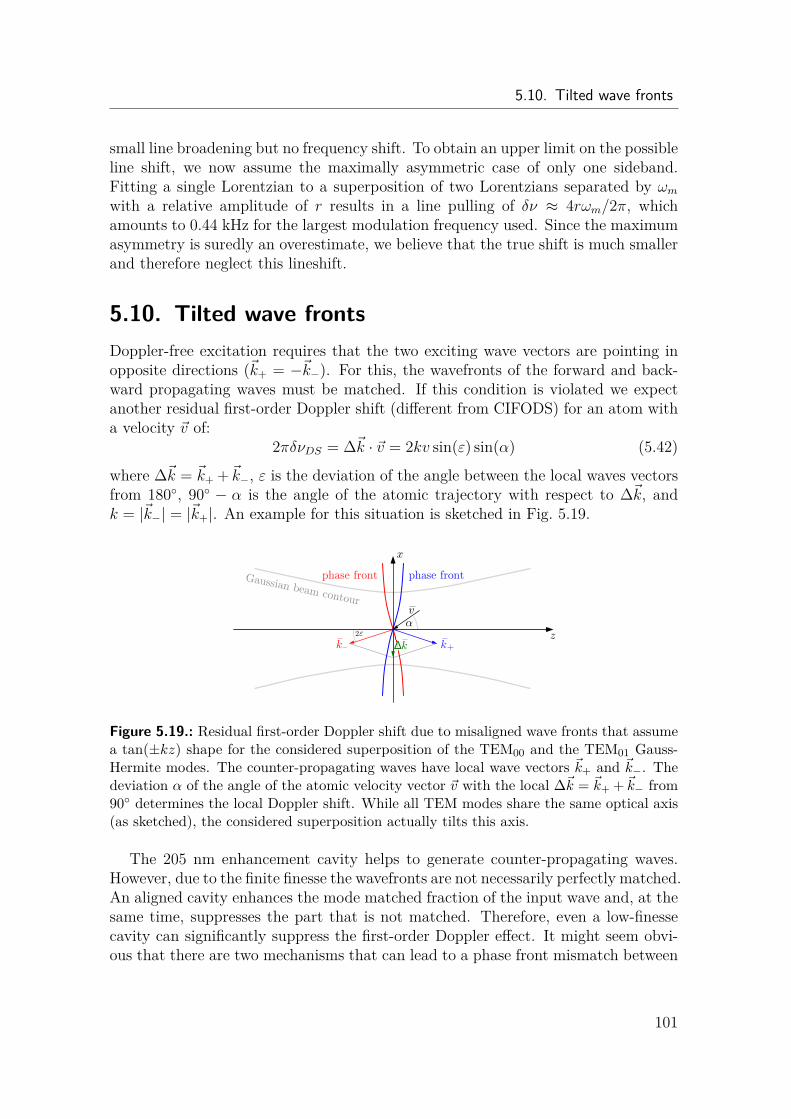
5.10. Tilted wave fronts
small line broadening but no frequency shift. To obtain an upper limit on the possibleline shift, we now assume the maximally asymmetric case of only one sideband.Fitting a single Lorentzian to a superposition of two Lorentzians separated by ωmwith a relative amplitude of r results in a line pulling of δν ≈ 4rωm/2π, whichamounts to 0.44 kHz for the largest modulation frequency used. Since the maximumasymmetry is suredly an overestimate, we believe that the true shift is much smallerand therefore neglect this lineshift.
5.10. Tilted wave frontsDoppler-free excitation requires that the two exciting wave vectors are pointing inopposite directions (~k+ = −~k−). For this, the wavefronts of the forward and back-ward propagating waves must be matched. If this condition is violated we expectanother residual first-order Doppler shift (different from CIFODS) for an atom witha velocity ~v of:
2πδνDS = ∆~k · ~v = 2kv sin(ε) sin(α) (5.42)
where ∆~k = ~k+ +~k−, ε is the deviation of the angle between the local waves vectorsfrom 180, 90 − α is the angle of the atomic trajectory with respect to ∆~k, andk = |~k−| = |~k+|. An example for this situation is sketched in Fig. 5.19.
x
zk+
2
vα
phase frontphase frontGaussian beam contour
k—
ε
∆k
Figure 5.19.: Residual first-order Doppler shift due to misaligned wave fronts that assumea tan(±kz) shape for the considered superposition of the TEM00 and the TEM01 Gauss-Hermite modes. The counter-propagating waves have local wave vectors ~k+ and ~k−. Thedeviation α of the angle of the atomic velocity vector ~v with the local ∆~k = ~k+ +~k− from90 determines the local Doppler shift. While all TEM modes share the same optical axis(as sketched), the considered superposition actually tilts this axis.
The 205 nm enhancement cavity helps to generate counter-propagating waves.However, due to the finite finesse the wavefronts are not necessarily perfectly matched.An aligned cavity enhances the mode matched fraction of the input wave and, at thesame time, suppresses the part that is not matched. Therefore, even a low-finessecavity can significantly suppress the first-order Doppler effect. It might seem obvi-ous that there are two mechanisms that can lead to a phase front mismatch between
101
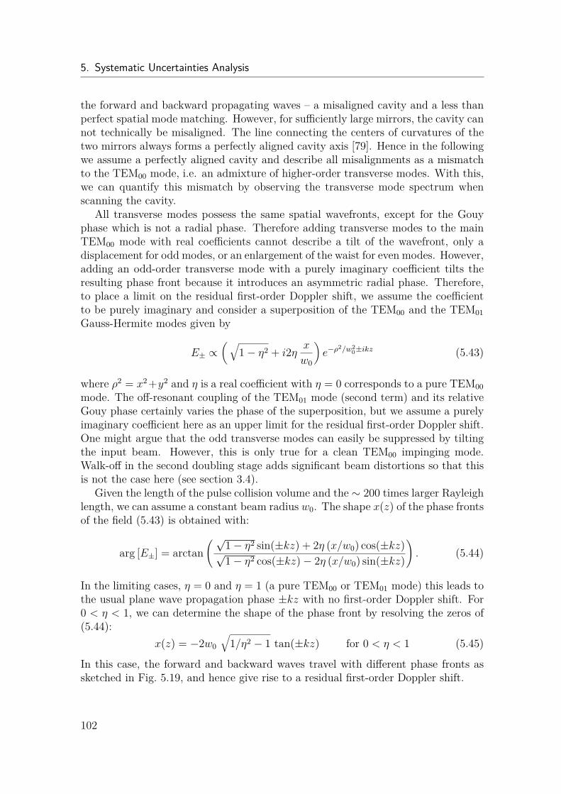
5. Systematic Uncertainties Analysis
the forward and backward propagating waves – a misaligned cavity and a less thanperfect spatial mode matching. However, for sufficiently large mirrors, the cavity cannot technically be misaligned. The line connecting the centers of curvatures of thetwo mirrors always forms a perfectly aligned cavity axis [79]. Hence in the followingwe assume a perfectly aligned cavity and describe all misalignments as a mismatchto the TEM00 mode, i.e. an admixture of higher-order transverse modes. With this,we can quantify this mismatch by observing the transverse mode spectrum whenscanning the cavity.
All transverse modes possess the same spatial wavefronts, except for the Gouyphase which is not a radial phase. Therefore adding transverse modes to the mainTEM00 mode with real coefficients cannot describe a tilt of the wavefront, only adisplacement for odd modes, or an enlargement of the waist for even modes. However,adding an odd-order transverse mode with a purely imaginary coefficient tilts theresulting phase front because it introduces an asymmetric radial phase. Therefore,to place a limit on the residual first-order Doppler shift, we assume the coefficientto be purely imaginary and consider a superposition of the TEM00 and the TEM01Gauss-Hermite modes given by
E± ∝(√
1− η2 + i2η x
w0
)e−ρ
2/w20±ikz (5.43)
where ρ2 = x2 +y2 and η is a real coefficient with η = 0 corresponds to a pure TEM00mode. The off-resonant coupling of the TEM01 mode (second term) and its relativeGouy phase certainly varies the phase of the superposition, but we assume a purelyimaginary coefficient here as an upper limit for the residual first-order Doppler shift.One might argue that the odd transverse modes can easily be suppressed by tiltingthe input beam. However, this is only true for a clean TEM00 impinging mode.Walk-off in the second doubling stage adds significant beam distortions so that thisis not the case here (see section 3.4).
Given the length of the pulse collision volume and the ∼ 200 times larger Rayleighlength, we can assume a constant beam radius w0. The shape x(z) of the phase frontsof the field (5.43) is obtained with:
arg [E±] = arctan( √
1− η2 sin(±kz) + 2η (x/w0) cos(±kz)√1− η2 cos(±kz)− 2η (x/w0) sin(±kz)
). (5.44)
In the limiting cases, η = 0 and η = 1 (a pure TEM00 or TEM01 mode) this leads tothe usual plane wave propagation phase ±kz with no first-order Doppler shift. For0 < η < 1, we can determine the shape of the phase front by resolving the zeros of(5.44):
x(z) = −2w0
√1/η2 − 1 tan(±kz) for 0 < η < 1 (5.45)
In this case, the forward and backward waves travel with different phase fronts assketched in Fig. 5.19, and hence give rise to a residual first-order Doppler shift.
102
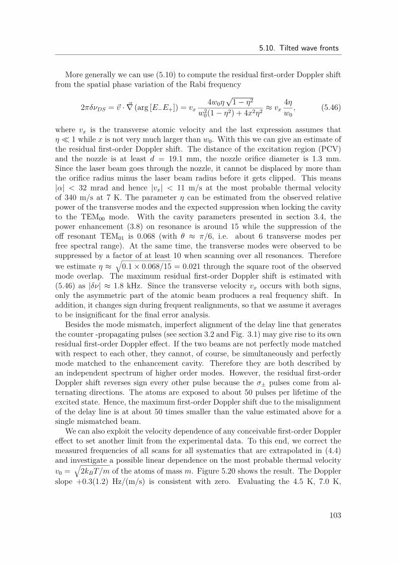
5.10. Tilted wave fronts
More generally we can use (5.10) to compute the residual first-order Doppler shiftfrom the spatial phase variation of the Rabi frequency
2πδνDS = ~v · ~∇ (arg [E−E+]) = vx4w0η
√1− η2
w20(1− η2) + 4x2η2 ≈ vx
4ηw0, (5.46)
where vx is the transverse atomic velocity and the last expression assumes thatη 1 while x is not very much larger than w0. With this we can give an estimate ofthe residual first-order Doppler shift. The distance of the excitation region (PCV)and the nozzle is at least d = 19.1 mm, the nozzle orifice diameter is 1.3 mm.Since the laser beam goes through the nozzle, it cannot be displaced by more thanthe orifice radius minus the laser beam radius before it gets clipped. This means|α| < 32 mrad and hence |vx| < 11 m/s at the most probable thermal velocityof 340 m/s at 7 K. The parameter η can be estimated from the observed relativepower of the transverse modes and the expected suppression when locking the cavityto the TEM00 mode. With the cavity parameters presented in section 3.4, thepower enhancement (3.8) on resonance is around 15 while the suppression of theoff resonant TEM01 is 0.068 (with θ ≈ π/6, i.e. about 6 transverse modes perfree spectral range). At the same time, the transverse modes were observed to besuppressed by a factor of at least 10 when scanning over all resonances. Thereforewe estimate η ≈
√0.1× 0.068/15 = 0.021 through the square root of the observed
mode overlap. The maximum residual first-order Doppler shift is estimated with(5.46) as |δν| ≈ 1.8 kHz. Since the transverse velocity vx occurs with both signs,only the asymmetric part of the atomic beam produces a real frequency shift. Inaddition, it changes sign during frequent realignments, so that we assume it averagesto be insignificant for the final error analysis.
Besides the mode mismatch, imperfect alignment of the delay line that generatesthe counter -propagating pulses (see section 3.2 and Fig. 3.1) may give rise to its ownresidual first-order Doppler effect. If the two beams are not perfectly mode matchedwith respect to each other, they cannot, of course, be simultaneously and perfectlymode matched to the enhancement cavity. Therefore they are both described byan independent spectrum of higher order modes. However, the residual first-orderDoppler shift reverses sign every other pulse because the σ± pulses come from al-ternating directions. The atoms are exposed to about 50 pulses per lifetime of theexcited state. Hence, the maximum first-order Doppler shift due to the misalignmentof the delay line is at about 50 times smaller than the value estimated above for asingle mismatched beam.
We can also exploit the velocity dependence of any conceivable first-order Dopplereffect to set another limit from the experimental data. To this end, we correct themeasured frequencies of all scans for all systematics that are extrapolated in (4.4)and investigate a possible linear dependence on the most probable thermal velocityv0 =
√2kBT/m of the atoms of mass m. Figure 5.20 shows the result. The Doppler
slope +0.3(1.2) Hz/(m/s) is consistent with zero. Evaluating the 4.5 K, 7.0 K,
103
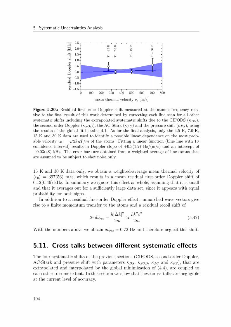
5. Systematic Uncertainties Analysis
Figure 5.20.: Residual first-order Doppler shift measured at the atomic frequency rela-tive to the final result of this work determined by correcting each line scan for all othersystematic shifts including the extrapolated systematic shifts due to the CIFODS (κDS),the second-order Doppler (κSOD), the AC-Stark (κAC) and the pressure shift (κPS), usingthe results of the global fit in table 4.1. As for the final analysis, only the 4.5 K, 7.0 K,15 K and 30 K data are used to identify a possible linear dependence on the most prob-able velocity v0 =
√2kBT/m of the atoms. Fitting a linear function (blue line with 1σ
confidence interval) results in Doppler slope of +0.3(1.2) Hz/(m/s) and an intercept of−0.03(48) kHz. The error bars are obtained from a weighted average of lines scans thatare assumed to be subject to shot noise only.
15 K and 30 K data only, we obtain a weighted-average mean thermal velocity of〈v0〉 = 397(56) m/s, which results in a mean residual first-order Doppler shift of0.12(0.46) kHz. In summary we ignore this effect as whole, assuming that it is smalland that it averages out for a sufficiently large data set, since it appears with equalprobability for both signs.
In addition to a residual first-order Doppler effect, unmatched wave vectors giverise to a finite momentum transfer to the atoms and a residual recoil shift of
2πδνrec = ~|∆k|22m ≈ ~k2ε2
2m (5.47)
With the numbers above we obtain δνrec = 0.72 Hz and therefore neglect this shift.
5.11. Cross-talks between different systematic effectsThe four systematic shifts of the previous sections (CIFODS, second-order Doppler,AC-Stark and pressure shift with parameters κDS, κSOD, κAC and κPS), that areextrapolated and interpolated by the global minimization of (4.4), are coupled toeach other to some extent. In this section we show that these cross-talks are negligibleat the current level of accuracy.
104
5.11. Cross-talks between different systematic effects
SOD/AC-Stark: Just like the AC-Stark shift, the SOD shift depends slightly onthe laser power. This is because an additional 205 nm photon can ionize the3S level. Slower atoms are more prone to ionization since they stay longer inthe laser field. The laser intensity scaling for the AC-Stark shift and ionizationis not the same (quadratic vs. cubic). The result is a laser power dependenceof the SOD shift. Ignoring this dependence in (4.4) leads to a systematicshift that we estimate by comparing two Monte Carlo simulations using thesame set of atomic trajectories. With one, we extrapolate to zero laser powerusing the global minimization (as in the experiment) with realistic experimentalconditions. In the second, we turn off the AC-Stark effect by setting βACin (5.13) and (2.43) to zero. Then we run the same minimization withoutκAC . The frequency difference of the two simulations is less than 3 Hz for alltemperatures between T = 1 . . . 200 K.
In another simulation we use separate parameters, κAC , for different tempera-tures instead of a global one. Using realistic experimental conditions, but withthe chirp parameter set to zero and the nozzle distance fixed to d = 19.1 mm,we find that the resulting differences of the extracted absolute frequencies arebelow 0.1 Hz for all nozzle temperatures T ≤ 180 K. With that, we concludethat it is safe to ignore the SOD/AC-Stark cross-talk in our data analysis.
SOD/CIFODS: Faster atoms with a larger SOD shift deposit their fluorescencelight further downstream of the atomic beam, which mimics a CIFODS withour detection scheme. This has already been discussed in Fig. 5.2 with thecorresponding simulation data and is repeated in Fig. 5.21. As discussed insection 5.1, the compensation of the CIFODS is based on the assumption thatit is linear in the chirp parameter b (see (5.6)). Adding a SOD induced spu-rious offset to the chirp parameter ∆b does not effect this linearity and leadsto exactly the same compensation method (5.7). The unperturbed transitionfrequency comes out correctly, but the (irrelevant) chirp parameter does not.This assumes that ∆b is constant across the PCV, a feature that cannot beread from Fig. 5.21. However, we can use it to read off the range of SODshifts covered by the auxiliary detectors, i.e. f2− f3, and multiply by κDS (see(5.6)) to obtain an estimate of the linear SOD induced spurious CIFODS of400 Hz × 0.043 = 17 Hz at T = 7 K. For larger temperatures, the position de-pendent SOD difference between f2 and f3 increases linearly, reaching ≈ 74 Hzat T = 30 K. With regard to Fig. 5.21, we expect the nonlinear contributionto be even smaller.
This cross-talk can again be estimated by selectively turning some effects offin the Monte Carlo simulations and running them with the same set of atomictrajectories. In this case, we turned off the AC-Stark effect and keep the nozzledistance at d = 19.1 mm. We run the simulations with T = 1 . . . 200 K andwith a range b = −0.1, 0.0,+0.1 extrapolating to zero temperature. Comparing
105
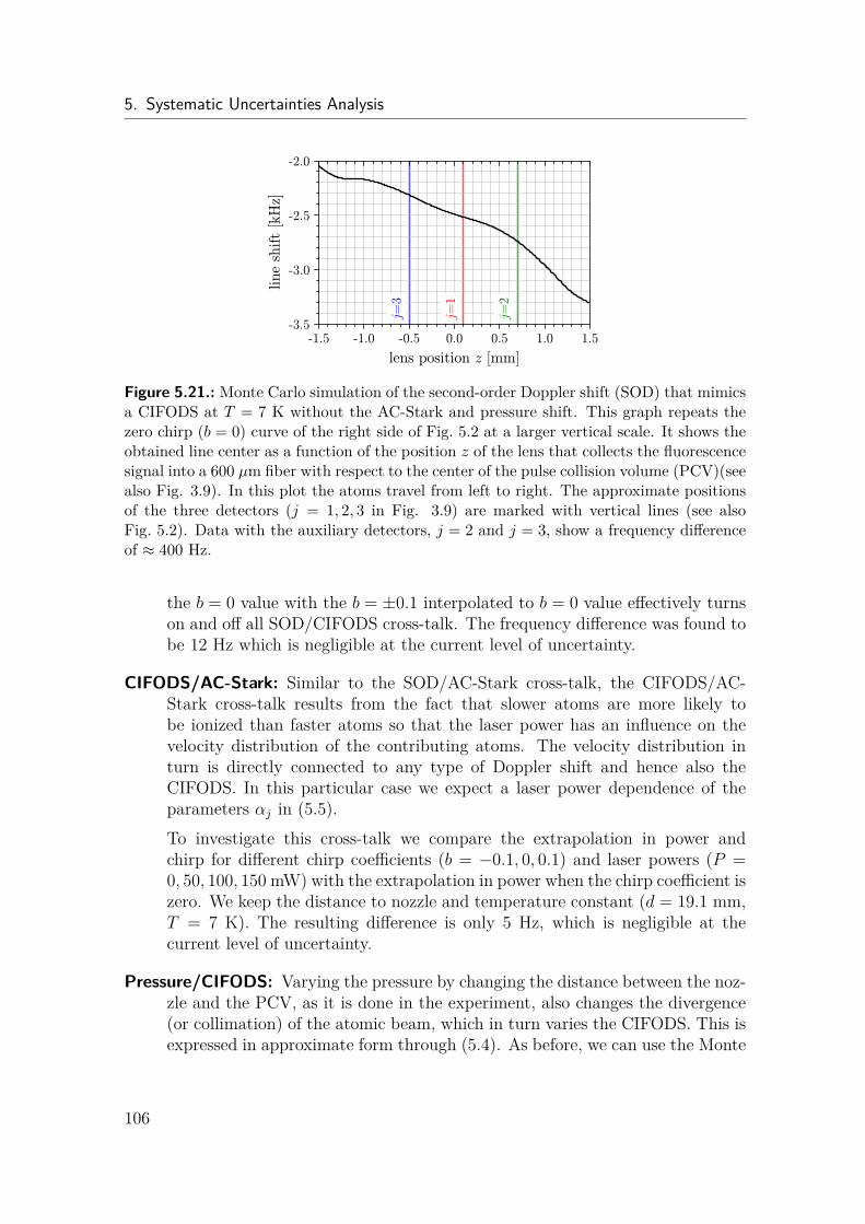
5. Systematic Uncertainties Analysis
Figure 5.21.: Monte Carlo simulation of the second-order Doppler shift (SOD) that mimicsa CIFODS at T = 7 K without the AC-Stark and pressure shift. This graph repeats thezero chirp (b = 0) curve of the right side of Fig. 5.2 at a larger vertical scale. It shows theobtained line center as a function of the position z of the lens that collects the fluorescencesignal into a 600 µm fiber with respect to the center of the pulse collision volume (PCV)(seealso Fig. 3.9). In this plot the atoms travel from left to right. The approximate positionsof the three detectors (j = 1, 2, 3 in Fig. 3.9) are marked with vertical lines (see alsoFig. 5.2). Data with the auxiliary detectors, j = 2 and j = 3, show a frequency differenceof ≈ 400 Hz.
the b = 0 value with the b = ±0.1 interpolated to b = 0 value effectively turnson and off all SOD/CIFODS cross-talk. The frequency difference was found tobe 12 Hz which is negligible at the current level of uncertainty.
CIFODS/AC-Stark: Similar to the SOD/AC-Stark cross-talk, the CIFODS/AC-Stark cross-talk results from the fact that slower atoms are more likely tobe ionized than faster atoms so that the laser power has an influence on thevelocity distribution of the contributing atoms. The velocity distribution inturn is directly connected to any type of Doppler shift and hence also theCIFODS. In this particular case we expect a laser power dependence of theparameters αj in (5.5).To investigate this cross-talk we compare the extrapolation in power andchirp for different chirp coefficients (b = −0.1, 0, 0.1) and laser powers (P =0, 50, 100, 150 mW) with the extrapolation in power when the chirp coefficient iszero. We keep the distance to nozzle and temperature constant (d = 19.1 mm,T = 7 K). The resulting difference is only 5 Hz, which is negligible at thecurrent level of uncertainty.
Pressure/CIFODS: Varying the pressure by changing the distance between the noz-zle and the PCV, as it is done in the experiment, also changes the divergence(or collimation) of the atomic beam, which in turn varies the CIFODS. This isexpressed in approximate form through (5.4). As before, we can use the Monte
106
5.11. Cross-talks between different systematic effects
Carlo simulation to model the CIFODS dependence on the atomic beam col-limation within the PCV more accurately. However, we do not model thepressure shift with our Monte Carlo code (see section 2.5). Nevertheless, wecan get partial information on the pressure/CIFODS cross-talk from it. Forthis purpose we use again the simulation data generated under realistic expe-rimental conditions and analyze it like the experimental data, but in this caseseparately for the two nozzle distances d = 19.1 mm and d = 27.1 mm andwith two separate CIFODS coefficients κDS. We then compare the absolutefrequencies obtained in this way by an analysis that uses only a common co-efficient κDS as was done for the real data analysis. The comparison gives anestimate of the pressure/CIFODS cross-talk assuming that the pressure shift isindependent of the atomic beam divergence (see below). We performed thesetests at all temperatures used in the experimental data evaluation (T ≤ 30 K)and obtain typical differences between the sets of ≈ 4 Hz (T = 7 K), ≈ 8 Hz(T = 15 K) and ≈ 24 Hz (T = 30 K). This is negligible at the current level ofuncertainty.
Pressure/SOD: There are several physical mechanisms that leads to a cross-talkbetween the SOD and the pressure shift. Since the SOD is mostly determinedby the temperature T of the nozzle, these would be a temperature dependenceof the pressure shift, or a temperature dependence of how we measure thepressure shift. The first mechanism is due to the 1/
√T dependence of the
number density n of particles in the beam. This is because we keep the totalflux into the nozzle constant but their escape velocity is proportional to 1/
√T .
Second, the cross-section of the collisional shift and collision rate, depends onvelocity. Third, the ratio of atomic vs. molecular hydrogen in the beam, i.e.the recombination rate, depends on temperature (see Fig. 3.8). This changesthe chemical composition of the beam. The fourth mechanism is a cross-talkbetween SOD shift and beam divergence, which mimics an intra-beam pressureshift with our measurement procedure based on the variation of the distancebetween the nozzle and the PCV.
The temperature dependence of the collisional shift is ∝ T−1/5 as obtained from(5.20) with n ∝ 1/
√T . The mean pressure shift is estimated to be 0.87 kHz
(see section 5.4). Using the uncertainties of the absolute frequency for thevarious nozzle temperatures as a weight, we compute the standard deviationof δνPS to 52 Hz. This is an error that we introduce in our data analysis byassuming that the pressure shift coefficient κPS is independent of temperature.
The cross-talk between the SOD and the beam divergence is actually not due tothe pressure shift itself but is rooted in the way we measure the pressure shift.Therefore we can use our Monte Carlos simulations to evaluate it, even thoughit does not describe the pressure shift. For this purpose we are comparing theresults from two Monte Carlo runs that are obtained with two nozzle distances
107
5. Systematic Uncertainties Analysis
and with b = 0 (no CIFODS) as well as the AC-Stark shift turned off. Dueto its large aspect ratio, atoms that cross the PCV under a large angle spendless time within it and, hence, the signal from the faster atoms along thesetrajectories is relatively enhanced. The faster atoms in turn experiences alarger SOD. The absolute frequencies deviate by only 1 Hz, which is negligibleat the current level of uncertainty.The evaluation of the temperature dependence of the degree of dissociationis difficult. According to our estimation (see section 5.4), the van-der-Waalscoefficient for atom-molecule collisions is of the same order of magnitude as foratom-atom collisions. However, the presence of the quadrupole electric field ofthe molecule decreases the pressure shift because it rather quenches the 3S statein hard collisions. Therefore, the shift from collisions with hydrogen moleculesis smaller than from collisions with atoms, and we neglect this mechanism.This suggests that even if the degree of dissociation changes with temperature,the dependence of the pressure shift is small.We can verify all of these effects and all other temperature couplings to the ab-solute frequency to some extent using the experimental data. For this purposewe perform the global minimization of (4.4) for each nozzle temperatures se-parately ignoring the SOD, i.e. by setting κSOD = 0. The CIFODS, AC-Starkshift and pressure shift are still compensated in this way but all temperature-dependent couplings are removed because the temperature is fixed. Finally, weextrapolate these results to zero temperature, and find that this result deviatesfrom the global fit (4.3) by 192 Hz only.
Pressure/AC-Stark: There are two mechanisms that cause a cross-talk between theAC-Stark shift and the pressure shift. Again, the collimation of the atomictrajectories that transverse the PCV changes with the nozzle distance. Thiscollimation possibly has an influence on the pressure shift giving rise to acontribution that is nonlinear in the atomic density. At the same time a largerdivergence leads to a relative increase of the number of atoms that sample thelower intensity radial fringes of the PCV. Secondly, ionization preferentiallyeffects atoms that travel closer to the optical axis where the density is higher.The pressure shift is the only systematics discussed in this work that is notincluded in our Monte Carlo simulation. Therefore we cannot estimate thiscross talk in this way. However, we assume that this cross-talk contributesonly a small correction and neglect it.It may seem conceivable that the normalization of the Doppler-free signal withthe Doppler-broadened signal (see sections 5.5 and 4.2), does not fully removethe laser power, Pi, dependence of the normalized line amplitudes, Ai, forwhatever reason. In that case the parameters κAC and κPS in (4.3) are notlinearly independent. This might be suspected to explain the discrepancybetween the experimentally determined AC-Stark shift and the theoretical
108
5.12. Results and Error Budget
value as described in section 5.2. To investigate this scenario, we have re-run the data evaluation fixing κPS = 0 and find for the AC-Stark coefficientκAC = 136.73 Hz/µW. This is compatible with the value from the global mi-nimization using all parameters (see table 4.1).
Estimating the cross-talk systematic shifts one-by-one has the advantage that oncan identify the largest contribution. After convincing ourselves that the items aboveare small individually, we can treat them all together in a Monte Carlo simulation(see next section). In this way we also include more complex cross-talks togetherwith line distortion effects (see previous sections). For this purpose we evaluatesimulation results obtained with realistic experimental conditions exactly like thereal experimental data. We obtain a deviation of only 24 Hz from the set frequencythat enters the simulation code. This “fitting model” uncertainty is included in theerror budget in table 5.1. We believe that this characterizes all systematic shiftthat have been discussed so far, except for the pressure shift, which was estimatedindependently. The purpose of listing the cross-talks above is to exclude possiblelarge and compensating systematic shifts that would require a much more carefulestimation.
5.12. Results and Error BudgetThe most straightforward, but not very transparent way to determine the overalluncertainty, is to generate an artificial data set with the Monte Carlo simulationsdescribed in the previous section, and analyse it in precisely the same the way asthe experimental data. Except for the pressure shift, we can include all systematiceffects in these simulations and vary the parameters such as the laser power and thechirp parameter in accordance with the experimental variation. In doing so, we finda total fitting model induced systematic shift of 24 Hz (see also section 5.11) whichwe include as an uncertainty into the error budget.
As detailed in section 4.4, we analyze the experimental data with a global mini-mization of (4.4) parameterizing the unperturbed transition frequency f0 and findfor the hyperfine centroid of the 1S-3S transition:
f1S-3S(centroid) = 2 922 743 278 665.79(72) kHz. (5.48)
Most of the systematic shifts are taken into account in the global minimization by co-efficients for the CIFODS, the second-order Doppler, the AC-Stark and the pressureshift κDS, κSOD, κAC and κPS respectively. With this minimization we extrapo-late and interpolate with noisy experimental data, so that the resulting uncertaintyshould be treated as a statistical uncertainty. In addition to this common estimate,we wish to obtain separate values for the systematic shifts – for example to determinethe best route for future improvements. We have already addressed some aspects ofindividual systematics in the discussions of section 5.
109
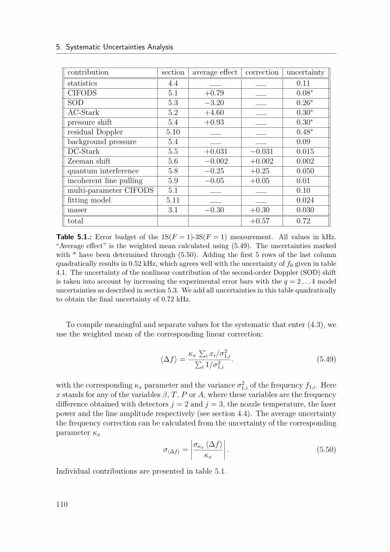
5. Systematic Uncertainties Analysis
contribution section average effect correction uncertaintystatistics 4.4 0.11CIFODS 5.1 +0.79 0.08∗SOD 5.3 −3.20 0.26∗AC-Stark 5.2 +4.60 0.30∗pressure shift 5.4 +0.93 0.30∗residual Doppler 5.10 0.48∗background pressure 5.4 0.09DC-Stark 5.5 +0.031 −0.031 0.015Zeeman shift 5.6 −0.002 +0.002 0.002quantum interference 5.8 −0.25 +0.25 0.050incoherent line pulling 5.9 −0.05 +0.05 0.01multi-parameter CIFODS 5.1 0.10fitting model 5.11 0.024maser 3.1 −0.30 +0.30 0.030total +0.57 0.72
Table 5.1.: Error budget of the 1S(F = 1)-3S(F = 1) measurement. All values in kHz.“Average effect” is the weighted mean calculated using (5.49). The uncertainties markedwith * have been determined through (5.50). Adding the first 5 rows of the last columnquadratically results in 0.52 kHz, which agrees well with the uncertainty of f0 given in table4.1. The uncertainty of the nonlinear contribution of the second-order Doppler (SOD) shiftis taken into account by increasing the experimental error bars with the q = 2 . . . 4 modeluncertainties as described in section 5.3. We add all uncertainties in this table quadraticallyto obtain the final uncertainty of 0.72 kHz.
To compile meaningful and separate values for the systematic that enter (4.3), weuse the weighted mean of the corresponding linear correction:
〈∆f〉 =κx
∑i xi/σ
21,i∑
i 1/σ21,i
. (5.49)
with the corresponding κx parameter and the variance σ21,i of the frequency f1,i. Here
x stands for any of the variables β, T , P or A, where these variables are the frequencydifference obtained with detectors j = 2 and j = 3, the nozzle temperature, the laserpower and the line amplitude respectively (see section 4.4). The average uncertaintythe frequency correction can be calculated from the uncertainty of the correspondingparameter κx
σ〈∆f〉 =∣∣∣∣∣σκx 〈∆f〉κx
∣∣∣∣∣ . (5.50)
Individual contributions are presented in table 5.1.
110
6. Conclusions and Outlook
6.1. Discussion of Measurement ResultsIn the course of this work, a high precision measurement of the 1S–3S transition(hyperfine component F = 1 → F = 1) has been performed. All corrections andthe error budget is given in table 5.1. After applying them to the mean transitionfrequency, we obtain the unperturbed absolute frequency:
f1S-3S(F =1) = 2 922 742 936 716.72(72) kHz (6.1)
Subtracting the hyperfine shifts of −341 949 069.6(8) Hz [10], gives the hyperfinecentroid:
f1S-3S(centroid) = 2 922 743 278 665.79(72) kHz (6.2)
It is in good agreement but more than 20 times more accurate than our previousroom temperature measurement [21]. It is 3.5 times more accurate than the previousmost precise 1S–3S measurement [7] (LKB, France) and disagrees by 2.1 combinedstandard deviations from it. Due to the improved uncertainty of our measurement,the combined standard deviation is almost entirely given by the uncertainty in [7].Since both experiments measure the same transition a discrepancy can not be due tothe theory. The probability (assuming Gaussian distributions) to find a discrepancyof 2.1σ is 3.4%. One may also think of some possible under-, overestimated orunexplored systematics in either one of experiments.
At the same time, we can use our result, the measured 1S-2S transition fre-quency [9], and QED in form of (1.4) to obtain a value for the Rydberg constant,which is twice as accurate as with all so far available hydrogen spectroscopy datacombined.
R∞ = 10973731.568226(38) m−1, (6.3)
and an independent value of the RMS proton charge radius
rp = 0.8482(38) fm. (6.4)
In doing so, we have used the collection of terms and the values for the fine struc-ture constant, as well as the electron-to-proton mass ratio given in the most recentpublished CODATA assembly [4]. More accurate values of these constants are avail-able [8], but that has no influence on the results presented here. Our value for theRydberg constant is more accurate than the most recent published CODATA value,but differs by 3.7 combined standard deviations from it. The proton charge radius
111
6. Conclusions and Outlook
disagrees by 2.9 combined standard deviations with the hydrogen world data as of2014, but is in better agreement with the most recent muonic value [16] and a recentmeasurement of the Lamb shift [6].
We have put our most effort to minimize the largest systematic effects as much aspossible. To this end the measurement has been performed at cryogenic temperaturesand this work constitutes the first cryogenic measurement of the 1S–3S transition inhydrogen. This reduces the residual first order Doppler shift (0.79 kHz, CIFODS).We have studied this new frequency comb spectroscopy inherent effect both exper-imentally and theoretically. Simple and intuitive formulas have been derived andcomprehensive Monte Carlo simulations performed. We found excellent agreementbetween theory and experiment (see section 5.1). In order to measure it experimen-tally, we have developed a flexible detector design, which upon the change of a singlefiber can significantly change its spatial detection profile and thus its sensitivity tothe chirp induced residual Doppler shift. Using several different detectors, the chirpinduced first order Doppler shift can be minimized and measured at the same time.We consider this method as the first step to fully spatially resolved frequency combspectroscopy, which we plan to extend with a single photon EMCCD camera. Sucha technique, where the transition frequency is resolved for different points in space,would lead to better understanding and instantaneous characterization of severalimportant effects.
One of the most troubling systematic shifts in high precision spectroscopy ex-periments is the second order Doppler shift (SOD) due to the unknown velocitydistribution, which is experimentally difficult to access . With a cryogenic atomicbeam also this effect could be reduced to -3.19 kHz only. To characterize the se-cond order Doppler shift, measurements at seven different temperatures from 4.5 Kto 180 K have been performed. The temperature dependence has been analyzedwith Maxwell-like velocity distributions by performing Monte Carlo simulations. Itwas found that a simple linear dependence describes the data best, despite some pre-dicted non-linearity at higher temperatures, if the Maxwellian velocity distribution isassumed. We believe that this shows the deviation from the Maxwellian distributionin atomic beams at low temperatures, such that the low velocity tail is suppressed.This data can be used in future experiments, to understand the velocity distribution,which inevitably limits the precision, when using atomic beams. Despite excellentagreement with the data, only temperatures below 30 K have been used for finalevaluation, in order to minimize any possible remaining non-linearities (see section5.3).
The collisional shift often constitutes only a small correction on the order of100 Hz, but is typically very difficult to measure experimentally. Therefore, it isoften only estimated theoretically and corrected. However, many uncertainties, suchas gas composition, exact pressure and its inhomogeneities within the interactionregion, have to be assumed. Therefore, despite an almost two-fold increase of thefinal uncertainty, we performed a direct measurement of this effect by varying thedistance between the interaction region and the hydrogen nozzle (see section 5.4).
112
6.2. Frequency Comb Spectroscopy Technique Investigation Results
This was possible due to a unique feature of the direct frequency comb spectroscopy,which limits the interaction region to a tiny volume, in which the pulses overlap.
The AC stark shift constitutes the largest systematic effect in our experiment(4.59 kHz on average). It has been measured experimentally by varying the in-tracavity laser power and extrapolating in the transmitted power. Nonlinearity isshown to be negligible (see appendix B). By performing several different separatemeasurements of the cavity waist and output mirror transmittivity (see. appendixA) and using Monte Carlo simulations, we obtained an AC Stark shift coefficient,which is about 3.5 times smaller than the experimental one. Some possible mistakein the determination of the waist or transmittivity of the mirror can possibly explainthis discrepancy, since the cavity is operated close to the instability region wherethe waist is difficult to measure. The mirrors are operated in vacuum with UV lightand are constantly flushed with oxygen, which also can influence the transmissionmeasurement. Also some undiscovered mistake in the calculation could be the cause.This is the major unknown of this measurement and needs further investigation.
We would like to stress that all systematic shifts, which we are aware of, are signi-ficantly smaller than the Proton Radius Puzzle discrepancy (7 kHz for 1S–3S), whichtogether with the result by our competitors at LKB [7], makes the 1S-3S measure-ments in hydrogen a unique test of the Proton Radius Puzzle. All significant effectsof this experiment have been measured experimentally using a simple interpolationor extrapolation, which is a very robust and simulation-independent method, as longas nonlinear terms can be shown to be negligible, which is extremely well justifiedfor the parameters of this experiment.
Two new experiments, which have been performed in our group are currently un-der evaluation. The 1S–3S centroid deuterium transition, using the same setup as forthis work, has the advantage of a significantly smaller AC Stark shift and two timessmaller second order Doppler shift. The measurement was done during the time ofthis work. The 2S–6P transition in hydrogen has been recently measured in ourgroup with sub kHz precision and is currently being analyzed and prepared for pub-lication. The corresponding 2S–6P measurement in deuterium is under preparation.Exciting contributions to the Proton Radius Puzzle and significant improvement ofthe Rydberg constant and the RMS proton charge radius are expected from theseexperiments.
6.2. Frequency Comb Spectroscopy TechniqueInvestigation Results
In the last two decades stabilized frequency combs became the standard tool forabsolute frequency determination in most precision labs around the globe [22], re-placing the tedious operation of long phase locked frequency chains. Their simplicityand broad wavelength coverage has been appreciated throughout the spectroscopycommunity and beyond it. T.W. Hänsch and J.L. Hall were honored in 2005 with
113
6. Conclusions and Outlook
the noble prize for their crucial contribution to this fundamentally important deve-lopment. Frequency combs found also numerous applications besides the absolutefrequency determination [23], [24]. The usage of frequency combs directly as excita-tion source for two-photon transitions, despite being one of the original ideas behindthe frequency comb [25], have not so far been applied in many precision spectroscopyexperiments.
This work is the first experimental demonstration of the Two-photon Direct Fre-quency Comb Spectroscopy below 1 kHz level [43, 80–83]. It shows that this tech-nique can be as precise as CW laser spectroscopy, offering several important advan-tages, which however come at a cost of a specific systematic residual Doppler shift.In this work, we have carefully analyzed and described the advantages and disad-vantages of this technique, its inherent systematic shifts and offered a technique tohandle them. The most apparent advantage is the possibility of generating UV andDUV laser sources through harmonics generation in crystals and gas targets, whereCW lasers with sufficient power are not available yet. This paves the way to pre-cision experiments with hydrogen-like ions, as for example anticipated in our groupwith the He+ spectroscopy [19] and many others. The confinement of the Doppler-free interaction region to a tiny volume with the size of the pulse length and thewaist of the beam, allows for separate Doppler-broadened fluorescence collection.We have shown that this can be used as efficient normalization signal, such thatalmost shot noise limited statistics can be reached, despite in this wavelength regionoften unavoidable laser power fluctuations as well as atomic flux fluctuations. Thesmall volume is further suitable for efficient light collection, efficient screenings ofelectric and magnetic fields. Pressure and field inhomogeneities are typically smallerand can be measured through a simple variation of the distance between the atomicsource and the pulse collision volume. The opposite side of an inherently confinedinteraction region is a reduced overall count rate and time-of-flight broadening, suchthat only at the center of the pulse collision volume and for very slow atoms, thesame count rate as with a CW laser with the same average power and beam size canbe reached. It can not be simply increased by collecting light from a larger part ofthe interaction region. The chirp induced first order Doppler shift has been discove-red in the course of this work [21] and was the limiting systematics for our previousroom temperature measurement. Its theory and comparison with experiment is dis-cussed in this work. A robust measurement method was developed, such that thisnew systematic frequency shift does not limit the precision and is not expected tobe the next largest systematics. Another important fundamental systematic shift,which can appear in both CW and frequency comb two-photon spectroscopy, whichwe refer to as Tilted Wave Front Doppler Shift is discussed in this work in section5.10. It explains the question, why the first order Doppler shift, despite cavity im-perfections, is strongly suppressed in two-photon spectroscopy. To our knowledge,this is the first detailed description of this effect.
114
6.3. Suggestions for Future Improvements
6.3. Suggestions for Future ImprovementsThe current 1S–3S measurement in hydrogen at the sub kilohertz level resolves theline width to only slightly more than 10−3, which is a quite moderate value, ascompared for instance to the 2S–4P measurement [5], where the resolution is pushedto 10−4 of the line width. The relatively narrow 1 MHz natural line width of the 1S–3S transition makes it very attractive for precision measurements (compare 20 MHzline width of the one-photon 2S-4P transition). Due to the cryogenic atomic beamand optimized design, many important systematic shifts such as the second orderDoppler shift and CIFODS are reduced. Other systematic shifts are under sufficientcontrol and can be efficiently measured and characterized. A comprehensive MonteCarlos simulation has been developed by Arthur Matveev in our group, which cananalyze in detail the experiment and systematic shifts. We believe therefore thatit is not unreasonable to push the limit of the uncertainty an order of magnitudefurther to the 100 Hz level, reaching the uncertainty for the RMS proton chargeradius, as given by the muonic hydrogen spectroscopy [3]. This is a challenging andfascinating goal. Suggestions on how the experiment can be improved are sketchedin this section.
By looking at the error budget table 5.1 the AC Stark shift is identified as thelargest effect in this experiment. It is on average 4.59 kHz (determined to 6.5%).Assuming same ratio of uncertainty to correction, one needs to reduce the AC Starkshift by about a factor of five to come well below the 100 Hz level. With a larger laserpower, the waist size could be increased by the same factor without losing signal,if one takes into account the larger number of interogated atoms. To increase thelaser power by a factor of five is a very challenging task. As explained in section3 commercial titanium:tapphire lasers operate at repetition rates around 80 MHz,such that we are forced to filter out every second comb mode by the SHG cavities, inorder to prevent incoherent line pulling (see section 5.9). We suggest to shorten thelaser cavity by a factor of two, while exchanging the active mode-locker (acousto-optic modulator) with one, which has its resonance frequency at 157.6 MHz. Thiswould increase the effective laser power at 820 nm by a factor of two and the fourthharmonic at 205 nm by a factor of four (first SHG cavity saturated, thus only linearincrease, second SHG quadratic). Another possibility to minimize the AC Starkshift, is to use an additional laser at a wavelength, where the AC Stark shift flipsthe sign (NIR region). The overall shift would be decreased, which still would needto be measured. However, in order for such a compensation to function, the spatialoverlap as well as intensity match within the entire interaction region between theexcitation laser and the compensating laser needs to be guaranteed. We believe,that this is a very difficult task to achieve. Another way to increase the fundamentalpower at 820 nm, is to use and external multi-pass titanium:sapphire amplifier.
In the current setup, Balmer-α fluorescence photons are collected with lenses andmulti-mode fibers and then guided to photo-multiplying tubes (Hamamatsu, H7421).The quantum efficiency at this wavelength is about 20% with 5 mm×5 mm active
115
6. Conclusions and Outlook
sensor area. We suggest instead to use a single photon EMCCD camera (electronmultiplying CCD, e.g. Andor Ixon 888), which exhibits 95% quantum efficiency and10 mm×10 mm sensor area. With this camera the total light collection efficiencycan be improved by a factor of 10 (5x higher QE and 2x larger solid angle). Further,the need for several separate detectors for CIFODS compensation is omitted, as eachpixel of the camera is essentially a separate detector. In order to keep the signal tonoise ratio (dominated by dark current and shot noise) at the current level of S/N =10, the 1024×1024 pixels need to be binned to 10×10 super pixels. We note, that itis not a trivial task, to design an objective with both a large solid angle and sufficientresolution and image depth. Compromises will need be made.
In the current setup, the atomic beam propagates along the laser beam axis,which reduces the time-of-flight broadening (PCV 600 µm long, while only 160 µmin diameter), such that almost natural line width is obtained for low temperatures(4.5 K and 7 K). However, collinear propagation of the atomic and the laser beams,necessitates a T-shaped nozzle (see fig. 3.1). Lothar Maisenbacher has performedsimulations, which showed, that in such a nozzle, hydrogen atoms collide few tensto hundreds times with the walls, where recombination with other hydrogen atomsoccurs. From our data (see section 3, fig. 3.8) we can estimate our dissociation ratioto around 10%. With an atomic beam propagating orthogonally to the laser beam,the number of wall collisions can be significantly reduced [54, 84], thus increasingthe dissociation ratio and the amount of hydrogen atoms in the beam. With lesscollisions however, also the velocity distribution could change. If at the same timethe waist is increased by roughly a factor of five (in order to reduce the AC Starkshift), the narrow line width can be preserved.
The second order Doppler shift is the second largest effect for this measurement(-3.19(26) kHz). Currently most data is measured at 7 K, while some data has beentaken at 4.5 K. With a suitable cryostat and thermal radiation shielding temperaturesat the level of 1–2 K can be reached, reducing the SOD shift to 300-600 Hz. However,as seen in figure 3.8 the count rate decreases very strongly at temperatures below≈ 30 K. This is because a thick layer of frozen molecular hydrogen forms inside thenozzle that atomic hydrogen diffuses into. The adsorption energy has been measuredto kB×38(5) K [84]. Once trapped inside the layer, atomic hydrogen recombines veryefficiently to molecules and the count rate drops. Though the actual count rate atsuch a temperature needs to be measured, a dramatic decrease is expected. With aproper nozzle for orthogonal atomic beam propagation this problem may be reduced.The necessity of lower temperatures underlines once again the need of better lightcollection and dissociation ratio increase. Further improvement of the second orderDoppler shift uncertainty can be made, if the velocity distribution is characterized aswas for instance recently done in [62]. In our opinion, the second order Doppler shiftis the most challenging systematics for an anticipated improvement of the 1S–3Smeasurement.
116
Appendix
A. Enhancement Cavity Characterization
A.1. Transmission MeasurementIn this chapter the characterization of the enhancement cavity of the 1S–3S hydrogenexperiment is presented and discussed. This is particularly important, since manysystematic shifts depend on the internal circulating power and the waist size of thecavity mode. In particular a comparison of the extrapolated AC Stark shift withsimulation is only possible if the transmission and waist size are known. The tiltedwave front Doppler shift is estimated relying on the knowledge of the mode structureand waist. Other effects such as second order Doppler shift also slightly depend onthe waist size and power, though these couplings have been found negligible at thecurrent level of uncertainty.
Figure A.1 shows our linear two-mirror enhancement cavity. The length is fixedat 0.9511 m by the repetition rate of the ps-comb (157.6 MHz). The input couplingmirror M1 is mounted on a piezo transducer to lock the cavity using the dither locktechnique. The radii of curvature of both mirrors are specified by the manufacturer(Laseroptik) to ROC = 500(25) mm. The input coupler M1 has a transmission ofT1 = 6.4% and a reflectivity of around R1 = 90% while the backside mirror M2 hasa reflectivity of R2 = 97% with a very small transmission.
To measure the transmission of the backside mirror M2 we used the 205 nmlight of the ps-comb. We are interested in the total transmission through the mirror,MgF2 window (5 mm thickness), HR mirror (205 nm, 45, plane) and 90% PR mirror(205 nm, 5, plane), which guide the transmitted light onto the power meter, sincefrom the total transmission and the power recordings the circulating power can bededuced. The resulting value is Ttot = 0.00054(10). The uncertainty is estimatedfrom the calibration uncertainty of the power meter (Thorlabs S120VC, 7% at eachpower range, totaling 14%) and statistical uncertainty 6%. We have used two morepower meters to confirm this measurement. We have varied the polarization andfound no polarization dependence. We also increased the impinging intensity on themirror by means of an additional lens to verify intensity independent transmission.In this way we increased the intensity by about a factor of 15 (10 mW and 400 µmvs. 10 mW and 100 µm) making it comparable to the intensity, when the cavityis locked. We have measured the transmission of the mirror when the chamber
117
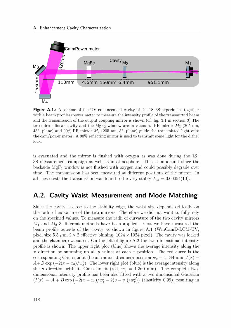
A. Enhancement Cavity Characterization
Cavity
Cam/Power meter
M1MgF2M3
M2
M4
951.1mm6.4mm4.6mm 150mm110mm
155mm
320mm
Figure A.1.: A scheme of the UV enhancement cavity of the 1S–3S experiment togetherwith a beam profiler/power meter to measure the intensity profile of the transmitted beamand the transmission of the output coupling mirror is shown (cf. fig. 3.1 in section 3) Thetwo-mirror linear cavity and the MgF2 window are in vacuum. HR mirror M3 (205 nm,45, plane) and 90% PR mirror M4 (205 nm, 5, plane) guide the transmitted light ontothe cam/power meter. A 90% reflecting mirror is used to transmit some light for the ditherlock.
is evacuated and the mirror is flushed with oxygen as was done during the 1S–3S measurement campaign as well as in atmosphere. This is important since thebackside MgF2 window is not flushed with oxygen and could possibly degrade overtime. The transmission has been measured at different positions of the mirror. Inall these tests the transmission was found to be very stably Ttot = 0.00054(10).
A.2. Cavity Waist Measurement and Mode MatchingSince the cavity is close to the stability edge, the waist size depends critically onthe radii of curvature of the two mirrors. Therefore we did not want to fully relyon the specified values. To measure the radii of curvature of the two cavity mirrorsM1 and M2 3 different methods have been applied. First we have measured thebeam profile outside of the cavity as shown in figure A.1 (WinCamD-LCM-UV,pixel size 5.5 µm, 2× 2 effective binning, 1024× 1024 pixel). The cavity was lockedand the chamber evacuated. On the left of figure A.2 the two-dimensional intensityprofile is shown. The upper right plot (blue) shows the average intensity along thex–direction by summing up all y–values at each x position. The red curve is thecorresponding Gaussian fit (beam radius at camera position wx = 1.344 mm, I(x) =A+B exp (−2(x− x0)/w2
x). The lower right plot (blue) is the average intensity alongthe y–direction with its Gaussian fit (red, wy = 1.360 mm). The complete two-dimensional intensity profile has been also fitted with a two-dimensional Gaussian(I(x) = A + B exp
(−2(x− x0)/w2
x − 2(y − y0)/w2y
)) (elasticity 0.99), resulting in
118
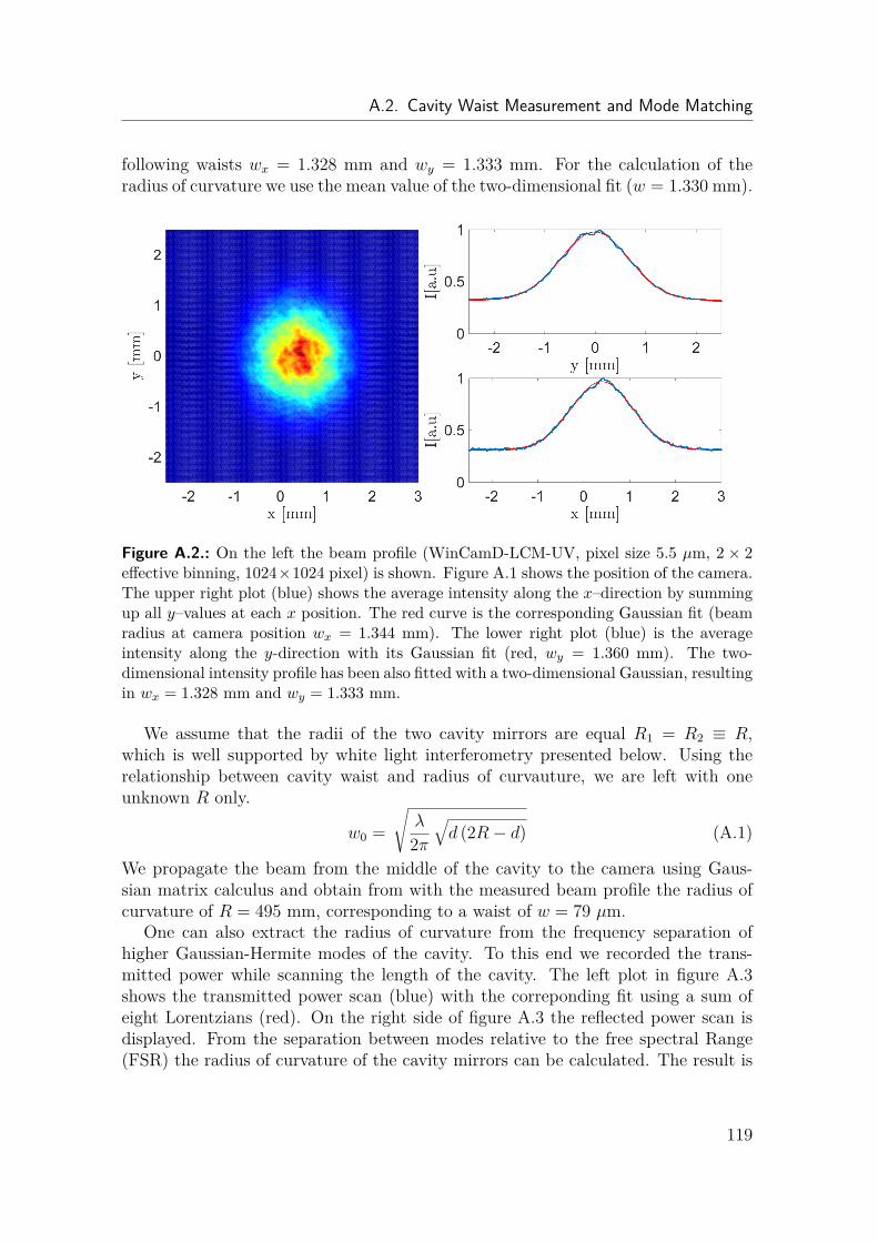
A.2. Cavity Waist Measurement and Mode Matching
following waists wx = 1.328 mm and wy = 1.333 mm. For the calculation of theradius of curvature we use the mean value of the two-dimensional fit (w = 1.330 mm).
Figure A.2.: On the left the beam profile (WinCamD-LCM-UV, pixel size 5.5 µm, 2 × 2effective binning, 1024×1024 pixel) is shown. Figure A.1 shows the position of the camera.The upper right plot (blue) shows the average intensity along the x–direction by summingup all y–values at each x position. The red curve is the corresponding Gaussian fit (beamradius at camera position wx = 1.344 mm). The lower right plot (blue) is the averageintensity along the y-direction with its Gaussian fit (red, wy = 1.360 mm). The two-dimensional intensity profile has been also fitted with a two-dimensional Gaussian, resultingin wx = 1.328 mm and wy = 1.333 mm.
We assume that the radii of the two cavity mirrors are equal R1 = R2 ≡ R,which is well supported by white light interferometry presented below. Using therelationship between cavity waist and radius of curvauture, we are left with oneunknown R only.
w0 =√λ
2π√d (2R− d) (A.1)
We propagate the beam from the middle of the cavity to the camera using Gaus-sian matrix calculus and obtain from with the measured beam profile the radius ofcurvature of R = 495 mm, corresponding to a waist of w = 79 µm.
One can also extract the radius of curvature from the frequency separation ofhigher Gaussian-Hermite modes of the cavity. To this end we recorded the trans-mitted power while scanning the length of the cavity. The left plot in figure A.3shows the transmitted power scan (blue) with the correponding fit using a sum ofeight Lorentzians (red). On the right side of figure A.3 the reflected power scan isdisplayed. From the separation between modes relative to the free spectral Range(FSR) the radius of curvature of the cavity mirrors can be calculated. The result is
119
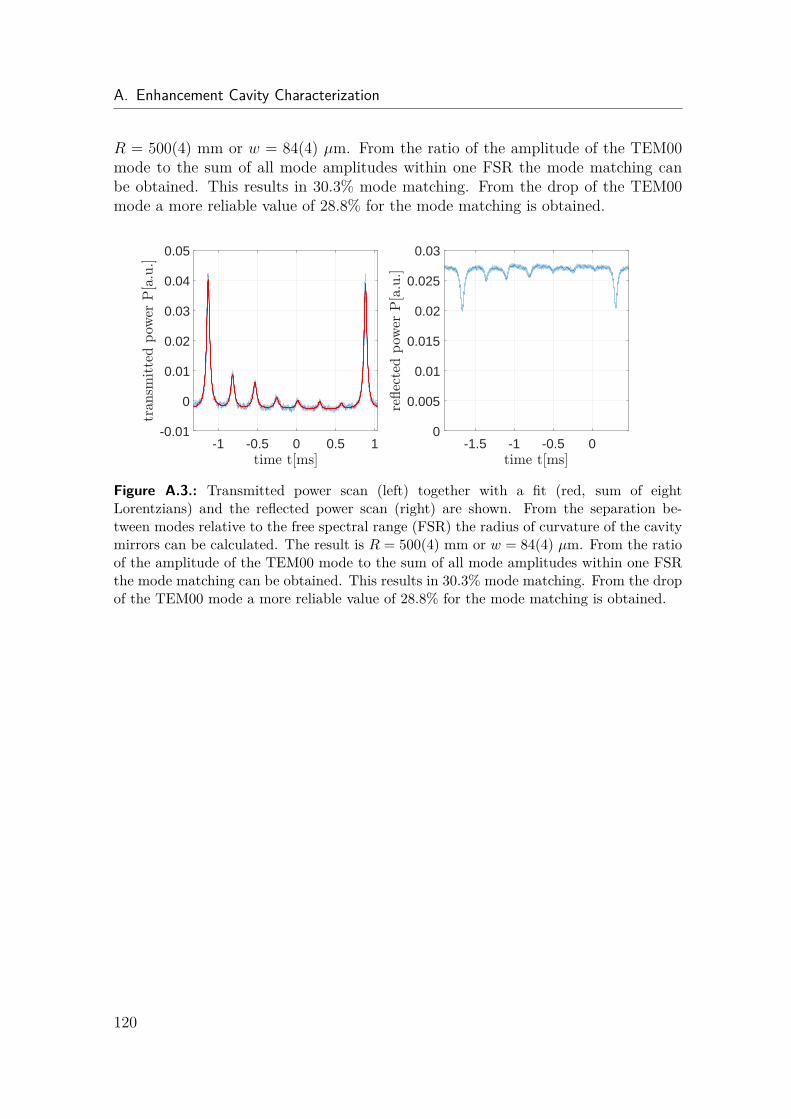
A. Enhancement Cavity Characterization
R = 500(4) mm or w = 84(4) µm. From the ratio of the amplitude of the TEM00mode to the sum of all mode amplitudes within one FSR the mode matching canbe obtained. This results in 30.3% mode matching. From the drop of the TEM00mode a more reliable value of 28.8% for the mode matching is obtained.
-1 -0.5 0 0.5 1-0.01
0
0.01
0.02
0.03
0.04
0.05
-1.5 -1 -0.5 00
0.005
0.01
0.015
0.02
0.025
0.03
Figure A.3.: Transmitted power scan (left) together with a fit (red, sum of eightLorentzians) and the reflected power scan (right) are shown. From the separation be-tween modes relative to the free spectral range (FSR) the radius of curvature of the cavitymirrors can be calculated. The result is R = 500(4) mm or w = 84(4) µm. From the ratioof the amplitude of the TEM00 mode to the sum of all mode amplitudes within one FSRthe mode matching can be obtained. This results in 30.3% mode matching. From the dropof the TEM00 mode a more reliable value of 28.8% for the mode matching is obtained.
120
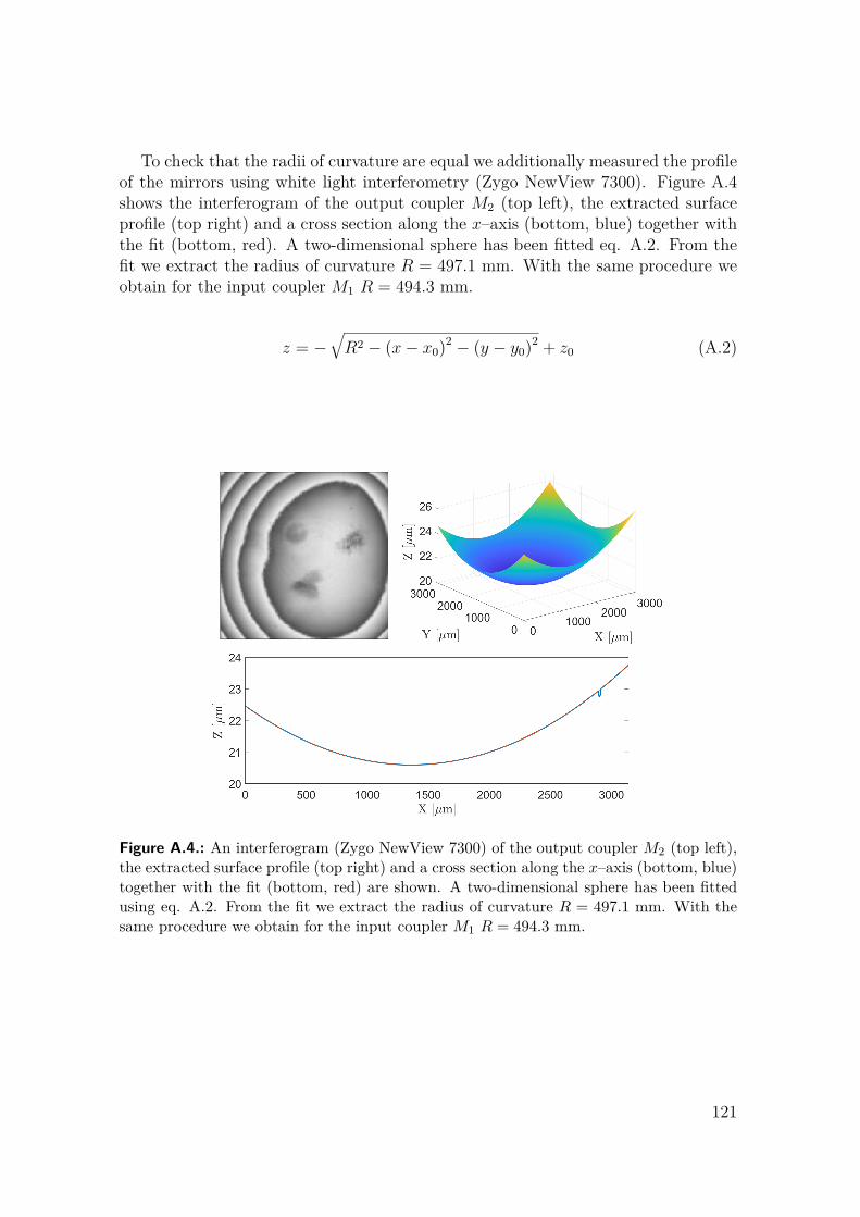
To check that the radii of curvature are equal we additionally measured the profileof the mirrors using white light interferometry (Zygo NewView 7300). Figure A.4shows the interferogram of the output coupler M2 (top left), the extracted surfaceprofile (top right) and a cross section along the x–axis (bottom, blue) together withthe fit (bottom, red). A two-dimensional sphere has been fitted eq. A.2. From thefit we extract the radius of curvature R = 497.1 mm. With the same procedure weobtain for the input coupler M1 R = 494.3 mm.
z = −√R2 − (x− x0)2 − (y − y0)2 + z0 (A.2)
Figure A.4.: An interferogram (Zygo NewView 7300) of the output coupler M2 (top left),the extracted surface profile (top right) and a cross section along the x–axis (bottom, blue)together with the fit (bottom, red) are shown. A two-dimensional sphere has been fittedusing eq. A.2. From the fit we extract the radius of curvature R = 497.1 mm. With thesame procedure we obtain for the input coupler M1 R = 494.3 mm.
121
B. AC Stark Shift Derivation
B. AC Stark Shift Derivation
B.1. Fourth Order AC Stark Shift
In this chapter the fourth order AC Stark shift (∝ I2) for CW laser and frequencycomb excitations is derived. It is import to verify that the non-linearity is negligible,since the linearity assumption is explicitly used for AC Stark shift extrapolation (seeseq. 5.2). As has been explained in section 2, the second order AC Stark shift (∝ I)for both the CW laser and frequency comb excitations compute from the averageintensity. This is a consequence of the linearity of the optical Bloch equations (seeeq. 2.43) and the fact that a frequency comb can be viewed as a superposition ofcomb modes. However nonlinear effects, such as the fourth order AC Stark shift, arestrongly enhanced if a frequency comb is used. It should be noted that odd orders ofthe AC Stark shift vanish. Further, due to its large spectral bandwidth, a frequencycomb can be resonant with one or several of the intermediate transitions, such thatadditional enhancement can occur. This derivation extends the derivation in [85].Consider the Hamiltonian H = H0 + V (ε, t), where H0 is the free Hamiltonian of thehydrogen atom or a hydrogen-like ion and V (ε, t) is the dipole interaction potentialof a laser field.
V (ε, t) = V e−ε|t| cos(ωt) (B.1)
The laser field is assumed to be a plane, monochromatic wave polarized along thez-direction, adiabatically damped in the distance past and future. In the interactionpicture VI(ε, t) = e
i~H0tV (ε, t)e− i
~H0t, we can calculate the time-evolution operatorUI(ε, t) using the Dyson series up to the fourth order.
Ui(ε, t) =1 +(− i~
)2 t∫−∞
dt′
t′∫
−∞
dt′′VI(ε, t
′)VI(ε, t′′)+
(− i~
)4 t∫−∞
dt′
t′∫
−∞
dt′′
t′′∫
−∞
dt′′′
t′′′∫
−∞
dt′′′′VI(ε, t
′)VI(ε, t′′)VI(ε, t
′′′)VI(ε, t′′′′)
(B.2)
All odd orders of the series vanish for states with the same parity. The secondorder is calculated in [85] for a CW laser and can be extended for a frequency comb
122
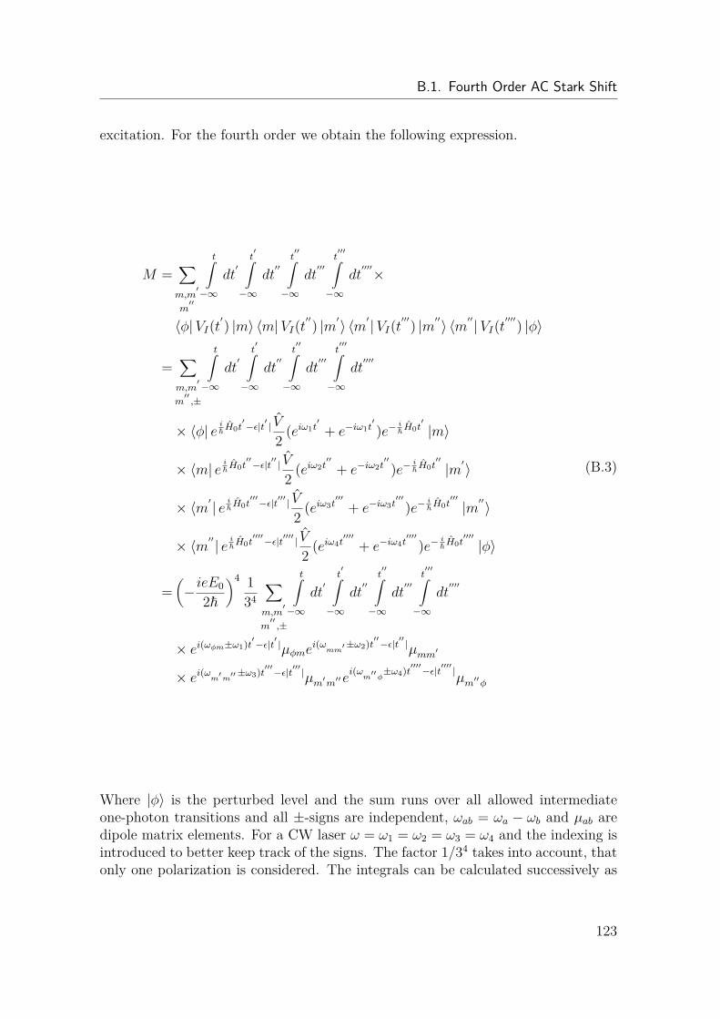
B.1. Fourth Order AC Stark Shift
excitation. For the fourth order we obtain the following expression.
M =∑m,m
′
m′′
t∫−∞
dt′
t′∫
−∞
dt′′
t′′∫
−∞
dt′′′
t′′′∫
−∞
dt′′′′×
〈φ|VI(t′) |m〉 〈m|VI(t
′′) |m′〉 〈m′ |VI(t′′′) |m′′〉 〈m′′|VI(t
′′′′) |φ〉
=∑m,m
′
m′′,±
t∫−∞
dt′
t′∫
−∞
dt′′
t′′∫
−∞
dt′′′
t′′′∫
−∞
dt′′′′
× 〈φ| ei~ H0t
′−ε|t′ | V
2 (eiω1t′
+ e−iω1t′
)e− i~ H0t
′
|m〉
× 〈m| ei~ H0t
′′−ε|t′′ | V
2 (eiω2t′′
+ e−iω2t′′
)e− i~ H0t
′′
|m′〉
× 〈m′| ei~ H0t
′′′−ε|t′′′ | V
2 (eiω3t′′′
+ e−iω3t′′′
)e− i~ H0t
′′′
|m′′〉
× 〈m′′ | ei~ H0t
′′′′−ε|t′′′′ | V
2 (eiω4t′′′′
+ e−iω4t′′′′
)e− i~ H0t
′′′′
|φ〉
=(−ieE0
2~
)4 134
∑m,m
′
m′′,±
t∫−∞
dt′
t′∫
−∞
dt′′
t′′∫
−∞
dt′′′
t′′′∫
−∞
dt′′′′
× ei(ωφm±ω1)t′−ε|t′ |µφmei(ω
mm′±ω2)t′′−ε|t′′ |µmm′
× ei(ωm′m
′′±ω3)t′′′−ε|t′′′ |µm′m′′ei(ω
m′′φ±ω4)t′′′′−ε|t′′′′ |
µm′′φ
(B.3)
Where |φ〉 is the perturbed level and the sum runs over all allowed intermediateone-photon transitions and all ±-signs are independent, ωab = ωa − ωb and µab aredipole matrix elements. For a CW laser ω = ω1 = ω2 = ω3 = ω4 and the indexing isintroduced to better keep track of the signs. The factor 1/34 takes into account, thatonly one polarization is considered. The integrals can be calculated successively as
123
B. AC Stark Shift Derivation
following:
M =(eE0
6~
)4 ∑m,m
′
m′′,±
t∫−∞
dt′
t′∫
−∞
dt′′
t′′∫−∞
dt′′′µφmµmm′µm′m′′µm′′φ
× ei(ωφm±ωφ)t′−ε|t′ |+i(ωmm
′±ω2)t′′−ε|t′′ |+i(ωm
′m
′′±ω3)t′′′−ε|t′′′ |
× ei(ω
m′′φ±ωφ)t′′′−ε|t′′′ |
i(ωm′′φ ± ωφ + iε)
=(eE0
6~
)4 ∑m,m
′
m′′,±
t∫−∞
dt′
t′∫
−∞
dt′′µφmµmm′µm′m′′µm′′φ
× ei(ωφm±ω1)t′−ε|t′ |+i(ωmm
′±ω2)t′′−ε|t′′ |
× ei(ω
m′φ±ω3±ω4)t′′−2ε|t′′ |
i(ωm′′φ ± ω4 + iε)i(ωm′
φ ± ω4 ± ω3 + 2iε)
=(eE0
6~
)4 ∑m,m
′
m′′,±
t∫−∞
dt′µφmµmm′µm′m′′µm′′φ
× ei(±ω1±ω2±ω3±ω4)t′−4ε|t′ |
i(ωm′′φ ± ω4 + iε)i(ωm′φ ± ω4 ± ω3 + 2iε)i(ωmφ ± ω4 ± ω3 ± ω2 + 3iε)
=(eE0
6~
)4 ∑m,m
′
m′′,±
µφmµmm′µm′m′′µm′′φ
× ei(±ω1±ω2±ω3±ω4)t′−4ε|t′ |
(ωm′′φ ± ω4 + iε)(ωm′φ ± ω4 ± ω3 + 2iε)
× 1(ωmφ ± ω4 ± ω3 ± ω2 + 3iε)(ω4 ± ω3 ± ω2 ± ω1 + 4iε)
(B.4)
Following [85] we compute ∂M/∂t, take the limit ε→ 0 and multiply by ~/i to obtainthe fourth order AC Stark shift of a particular level ∆EAC . We only use terms, whereω1±ω2±ω3±ω4 = 0. In this case there are six possible sign combinations (ω1ω2ω3ω4= + +−−,+−+1,−+ +−,+−−+,−+−+,−−++). If |φ〉 is an S-state, the firstintermediate state |m〉 has to be a P-state, the second |m′〉 an S-state or D-state,the third a P-state and the final state is again |φ〉. For |φ〉 being the 3S-state, thereis one close to resonance term in the denominator of B.4, ωφm′ ± ω3 ± ω4, if |m
′〉 isof of the 3D-states (D3/2 or D5/2) and ω3 = −ω4. The condition ω3 = −ω4 is fulfilled
124
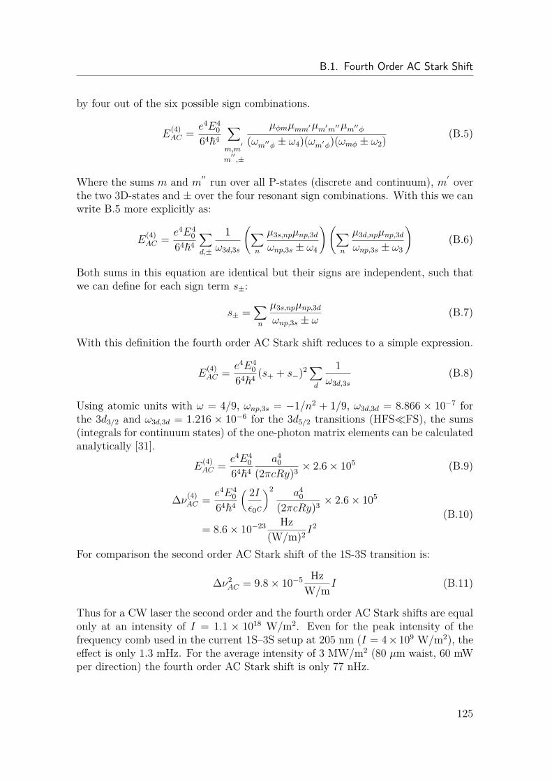
B.1. Fourth Order AC Stark Shift
by four out of the six possible sign combinations.
E(4)AC = e4E4
064~4
∑m,m
′
m′′,±
µφmµmm′µm′m′′µm′′φ
(ωm′′φ ± ω4)(ωm′φ)(ωmφ ± ω2) (B.5)
Where the sums m and m′′ run over all P-states (discrete and continuum), m′ overthe two 3D-states and ± over the four resonant sign combinations. With this we canwrite B.5 more explicitly as:
E(4)AC = e4E4
064~4
∑d,±
1ω3d,3s
(∑n
µ3s,npµnp,3dωnp,3s ± ω4
)(∑n
µ3d,npµnp,3dωnp,3s ± ω3
)(B.6)
Both sums in this equation are identical but their signs are independent, such thatwe can define for each sign term s±:
s± =∑n
µ3s,npµnp,3dωnp,3s ± ω
(B.7)
With this definition the fourth order AC Stark shift reduces to a simple expression.
E(4)AC = e4E4
064~4 (s+ + s−)2∑
d
1ω3d,3s
(B.8)
Using atomic units with ω = 4/9, ωnp,3s = −1/n2 + 1/9, ω3d,3d = 8.866 × 10⁻⁷ forthe 3d3/2 and ω3d,3d = 1.216 × 10⁻⁶ for the 3d5/2 transitions (HFSFS), the sums(integrals for continuum states) of the one-photon matrix elements can be calculatedanalytically [31].
E(4)AC = e4E4
064~4
a40
(2πcRy)3 × 2.6× 105 (B.9)
∆ν(4)AC = e4E4
064~4
( 2Iε0c
)2 a40
(2πcRy)3 × 2.6× 105
= 8.6× 10⁻²³ Hz(W/m)2 I
2(B.10)
For comparison the second order AC Stark shift of the 1S-3S transition is:
∆ν2AC = 9.8× 10⁻⁵ Hz
W/mI (B.11)
Thus for a CW laser the second order and the fourth order AC Stark shifts are equalonly at an intensity of I = 1.1 × 10¹⁸ W/m2. Even for the peak intensity of thefrequency comb used in the current 1S–3S setup at 205 nm (I = 4× 10⁹ W/m2), theeffect is only 1.3 mHz. For the average intensity of 3 MW/m2 (80 µm waist, 60 mWper direction) the fourth order AC Stark shift is only 77 nHz.
125
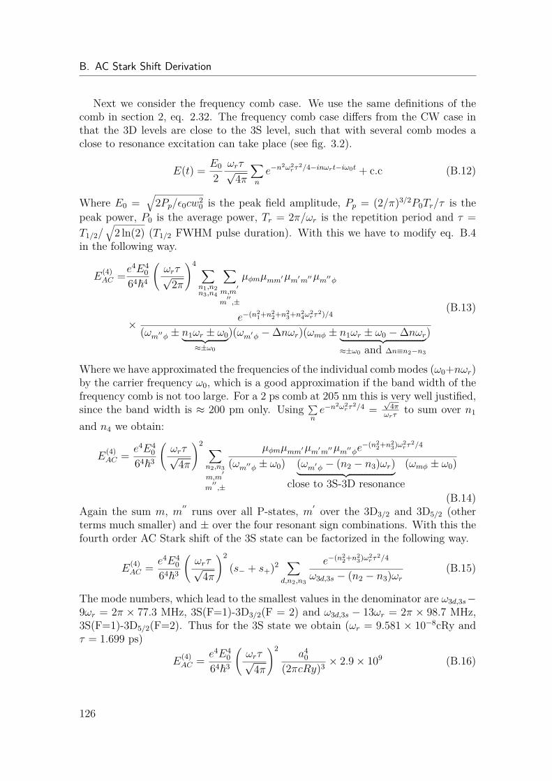
B. AC Stark Shift Derivation
Next we consider the frequency comb case. We use the same definitions of thecomb in section 2, eq. 2.32. The frequency comb case differs from the CW case inthat the 3D levels are close to the 3S level, such that with several comb modes aclose to resonance excitation can take place (see fig. 3.2).
E(t) = E0
2ωrτ√
4π∑n
e−n2ω2rτ
2/4−inωrt−iω0t + c.c (B.12)
Where E0 =√
2Pp/ε0cw20 is the peak field amplitude, Pp = (2/π)3/2P0Tr/τ is the
peak power, P0 is the average power, Tr = 2π/ωr is the repetition period and τ =T1/2/
√2 ln(2) (T1/2 FWHM pulse duration). With this we have to modify eq. B.4
in the following way.
E(4)AC =e
4E40
64~4
(ωrτ√
2π
)4 ∑n1,n2n3,n4
∑m,m
′
m′′,±
µφmµmm′µm′m′′µm′′φ
× e−(n21+n2
2+n23+n2
4ω2rτ
2)/4
(ωm′′φ ± n1ωr ± ω0︸ ︷︷ ︸≈±ω0
)(ωm′φ −∆nωr)(ωmφ ± n1ωr ± ω0 −∆nωr︸ ︷︷ ︸≈±ω0 and ∆n≡n2−n3
)
(B.13)
Where we have approximated the frequencies of the individual comb modes (ω0+nωr)by the carrier frequency ω0, which is a good approximation if the band width of thefrequency comb is not too large. For a 2 ps comb at 205 nm this is very well justified,since the band width is ≈ 200 pm only. Using ∑
ne−n
2ω2rτ
2/4 =√
4πωrτ
to sum over n1
and n4 we obtain:
E(4)AC = e4E4
064~3
(ωrτ√
4π
)2 ∑n2,n3m,m
′
m′′,±
µφmµmm′µm′m′′µm′′φe−(n2
2+n23)ω2
rτ2/4
(ωm′′φ ± ω0) (ωm′φ − (n2 − n3)ωr)︸ ︷︷ ︸close to 3S-3D resonance
(ωmφ ± ω0)
(B.14)Again the sum m, m′′ runs over all P-states, m′ over the 3D3/2 and 3D5/2 (otherterms much smaller) and ± over the four resonant sign combinations. With this thefourth order AC Stark shift of the 3S state can be factorized in the following way.
E(4)AC = e4E4
064~3
(ωrτ√
4π
)2
(s− + s+)2 ∑d,n2,n3
e−(n22+n2
3)ω2rτ
2/4
ω3d,3s − (n2 − n3)ωr(B.15)
The mode numbers, which lead to the smallest values in the denominator are ω3d,3s−9ωr = 2π × 77.3 MHz, 3S(F=1)-3D3/2(F = 2) and ω3d,3s − 13ωr = 2π × 98.7 MHz,3S(F=1)-3D5/2(F=2). Thus for the 3S state we obtain (ωr = 9.581 × 10⁻⁸cRy andτ = 1.699 ps)
E(4)AC = e4E4
064~3
(ωrτ√
4π
)2a4
0(2πcRy)3 × 2.9× 109 (B.16)
126
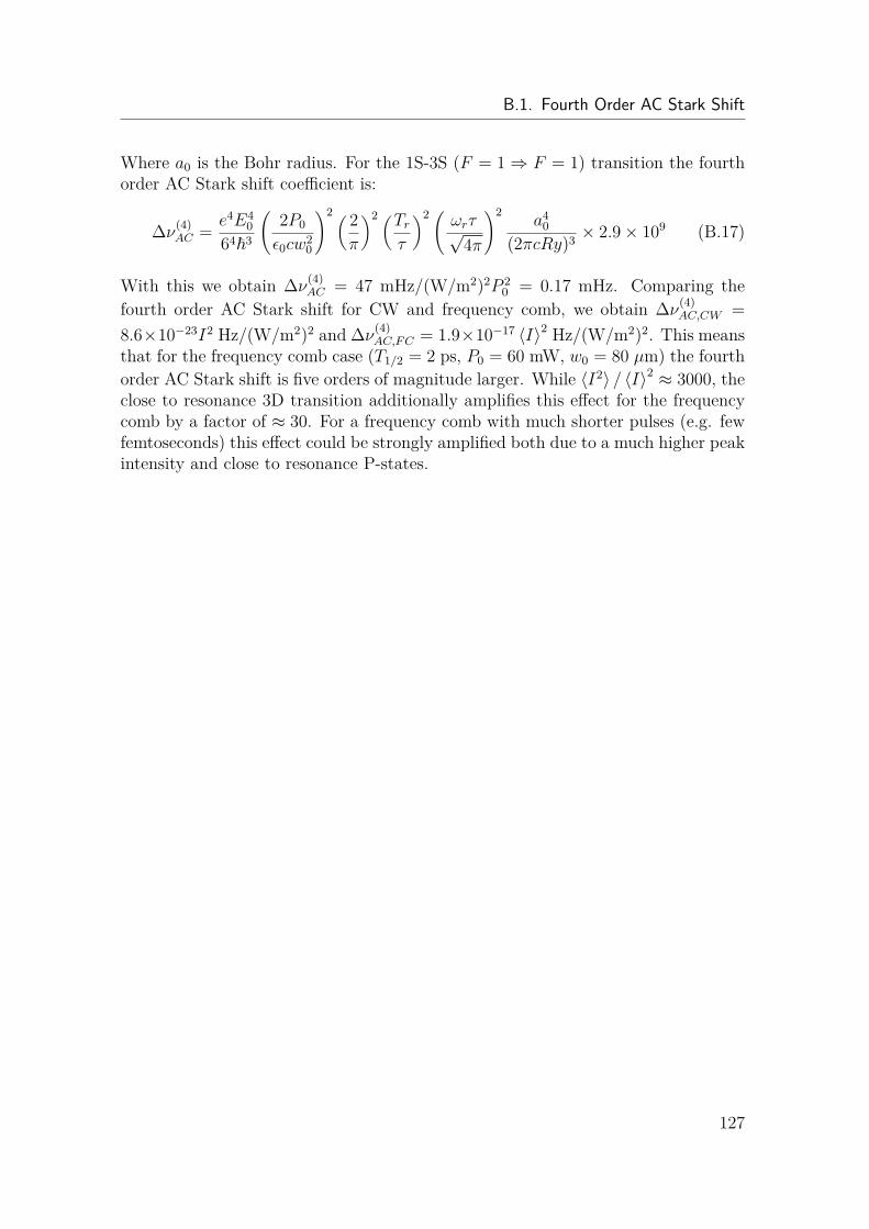
B.1. Fourth Order AC Stark Shift
Where a0 is the Bohr radius. For the 1S-3S (F = 1⇒ F = 1) transition the fourthorder AC Stark shift coefficient is:
∆ν(4)AC = e4E4
064~3
(2P0
ε0cw20
)2 ( 2π
)2 (Trτ
)2 ( ωrτ√4π
)2a4
0(2πcRy)3 × 2.9× 109 (B.17)
With this we obtain ∆ν(4)AC = 47 mHz/(W/m2)2P 2
0 = 0.17 mHz. Comparing thefourth order AC Stark shift for CW and frequency comb, we obtain ∆ν(4)
AC,CW =8.6×10⁻²³I2 Hz/(W/m2)2 and ∆ν(4)
AC,FC = 1.9×10⁻¹⁷ 〈I〉2 Hz/(W/m2)2. This meansthat for the frequency comb case (T1/2 = 2 ps, P0 = 60 mW, w0 = 80 µm) the fourthorder AC Stark shift is five orders of magnitude larger. While 〈I2〉 / 〈I〉2 ≈ 3000, theclose to resonance 3D transition additionally amplifies this effect for the frequencycomb by a factor of ≈ 30. For a frequency comb with much shorter pulses (e.g. fewfemtoseconds) this effect could be strongly amplified both due to a much higher peakintensity and close to resonance P-states.
127

Bibliography[1] R.H. Parker, C. Yu, W. Zhong, W. Estey, H. Müller, H. Measurement of the
fine-structure constant as a test of the Standard Model. Science 360, 191-195(2018).
[2] F. Heiße et al. High-precision measurement of the proton’s atomic mass. Phys.Rev. Lett. 119, 033001 (2017).
[3] R. Pohl et al. The size of the proton. Nature 466, 213-216 (2010).
[4] P.J. Mohr, D.B. Newell, B.N. Taylor, B.N. CODATA recommended values ofthe fundamental physical constants: 2014. Rev. Mod. Phys. 88, 035009 (2014).
[5] A. Beyer et al. The Rydberg constant and proton size from atomic hydrogen.Science 358, 79-85 (2017).
[6] N. Bezginov, T. Valdez, M. Horbatsch, A. Marsman, A.C. Vutha, E.A. Hessels,A measurement of the atomic hydrogen Lamb shift and the proton charge radius,Science 365, 1007-1012 (2019).
[7] H. Fleurbaey et al. New Measurement of the 1S-3S transition frequency ofhydrogen: contribution to the proton charge radius puzzle. Phys. Rev. Lett.120, 183001 (2018).
[8] see for example unpublished values at the NIST website:https://physics.nist.gov/cuu/Constants/index.html
[9] A. Matveev et al. Precision measurement of the hydrogen 1S-2S frequency viaa 920 km fiber link. Phys. Rev. Lett. 110, 230801 (2013).
[10] U.D. Jentschura, V.A. Yerokhin, Quantum electrodynamic corrections to thehyperfine structure of excited S states. Phys. Rev. A 73, 062503 (2006).
[11] Drake, Gordon W. F., Announcement: The Fundamental Role of PrecisionMeasurement in Atomic, Molecular, and Optical Physics. Phys. Rev. A. 98, 1(2018)
[12] Ångström, A. J., Recherches sur le spectre solaire : Spectre normal du soleil,atlas de six planches. (1868)
[13] Balmer, J. J., Notiz über die Spectrallinien des Wasserstoffes. Verhandlungender Naturforschenden Gesellschaft. 7, (1885)
129
Bibliography
[14] Michelson, A. A. and Morley, E. W., Notiz über die Spectrallinien des Wasser-stoffes. Phil. Mag. 5, 24 (1887)
[15] Cohen–Tannoudji, C., Diu, B. & Laboe F. Quantum Mechanics V2
[16] A. Antognini et al. Proton structure from the measurement of 2S-2P transitionfrequencies of muonic hydrogen. Science 339, 417-420 (2013).
[17] I.T. Lorenz, H.W. Hammer, U.G.Meißner, The size of the proton: Closing inon the radius puzzle. Eur. Phys. J. A 48, 151 (2012).
[18] G. Hagel, F. Nez, F. Biraben, Analysis and observation, on an atomic resonance,of the frequency shift due to the length modulation of an optical cavity. Appl.Opt. 41, 7702-7706 (2002).
[19] M. Herrmann et al. Feasibility of coherent XUV spectroscopy on the 1S-2Stransition in singly ionized helium. Phys. Rev. A 79, 052505 (2009).
[20] Arnoult, O., Nez, F., Julien, L. & Biraben, F. Optical frequency measurementof the 1S-3S two-photon transition in hydrogen. Eur. Phys. J. D 60, 2 (2010)
[21] D.C. Yost et al. Spectroscopy of the hydrogen 1S-3S transition with chirpedlaser pulses. Phys. Rev. A 93, 042509 (2016).
[22] Th. Udem, R. Holzwarth, T.W. Hänsch, Optical Frequency Metrology. Nature416, 233-237 (2004).
[23] Adler, F., Thorpe, M. J., Cossel, K. C. & Ye, J. Cavity-Enhanced Direct Fre-quency Comb Spectroscopy: Technology and Applications. Annu. Rev. Anal.Chem. 3, 1 (2010)
[24] M.C. Stowe et al. Direct frequency comb spectroscopy. Adv. Atom. Mol. Opt.Phy. 55, 1-60 (2008).
[25] Ye.V. Baklanov, V.P. Chebotayev, Narrow resonances of two-photon absorptionof super-narrow pulses in a gas. Appl. Phys. 12, 97-99 (1977).
[26] S. Reinhardt, E. Peters, T.W. Hänsch, Th. Udem, Two-photon direct frequencycomb spectroscopy with chirped pulses. Phys. Rev. A 81, 033427 (2010).
[27] Teets, R., Eckstein, J. & Hänsch, T. W.. Coherent two-photon excitation bymultiple light pulses. Phys. Rev. Lett. 38, 760–764 (1977)
[28] J.N. Eckstein, A.I. Ferguson, T.W. Hänsch, High-resolution two-photon spec-troscopy with picosecond light pulses. Phys. Rev, Lett. 40, 847-850 (1978).
[29] Thomas Udem, Habilitationsschrift, "Die Messung der Frequenz von Licht mitmodengekoppelten Lasern. (2002)
130
Bibliography
[30] M. Haas, U.D. Jentschura, C.M. Keitel, N. Kolachevsky, M. Herrmann, P.Fendel, M. Fischer, Th. Udem, R. Holzwarth, T.W. Hänsch, Two-photon exci-tation dynamics in bound two-body Coulomb systems including AC Stark shiftand ionization. Phys. Rev. A 73, 052501 (2006).
[31] Stobbe, M. Zur Quantenmechanik photoelektrischer Prozesse. Ann. Phys. 399,661–715 (1930)
[32] Edmonds, A. R., Angular momentum in quantum mechanics (1996)
[33] Bonin, K. D., & McIlrath, T. J. Two-photon electric-dipole selection rules. J.Opt. Soc. Am. B 1, 52 (1984)
[34] Peters, E. PhD Thesis. Experimental and theoretical investigation of directfrequency comb spectroscopy (2011)
[35] Matveev A. et al., To be published.
[36] H. Pauly, G. Scoles, (Ed.) Atomic and Molecular Beam Methods. (Oxford Uni-versity Press, New York, Oxford 1988).
[37] Th. Udem, Quantum electrodynamics and the proton size. Nat. Phys. 14, 632(2018).
[38] W. Xiong et al. A small proton charge radius from an electron–proton scatteringexperiment. Nature 575, 147-151 (2019).
[39] R.W.P. Drever, J.L. Hall, F.V. Kowalski, J. Hough, G.M. Ford, A.J. Munley,Laser phase and frequency stabilization using an optical resonator. Appl. Phys.B 31, 97-105 (1983).
[40] E. Peters, D.C. Yost, A. Matveev, T.W. Hänsch, Th. Udem, Frequency combspectroscopy of the hydrogen 1S-3S and 1S-3D transitions. Ann. d. Phys. 525,L29-L34 (2013).
[41] E. Peters, S.A. Diddams, P. Fendel, S. Reinhardt, T.W. Hänsch, Th. Udem, Adeep-UV optical frequency comb at 205 nm. Opt. Expr. 17, 9183-9190 (2009).
[42] G. Grynberg, F. Biraben, E. Giacobino, B. Cagnac, Doppler-free two-PhotonSpectroscopy of Neon. II. Line Intensities. J. de Phys. 38, 629-640 (1977).
[43] P. Fendel, S.D. Bergeson, Th. Udem, T.W. Hänsch, Two-photon frequency combspectroscopy of the 6s–8s transition in cesium. Opt. Lett. 32, 701-703 (2007).
[44] A. Ozawa, Y. Kobayashi, Chirped-pulse direct frequency-comb spectroscopy oftwo-photon transitions. Phys. Rev. A 86, 022514 (2012).
131
Bibliography
[45] H. Wang, A.M. Weiner, Efficiency of short-pulse type-I second-harmonic genera-tion with simultaneous spatial walk-off, temporal walk-off, and pump depletion.IEEE J. Quant. Electr. 39, 1600-1618 (2003).
[46] G. Hagel, R. Battesti, F. Nez, L. Julien, F. Biraben, Observation of a motionalStark effect to determine the second-order Doppler effect. Phys. Rev. Lett. 89,203001 (2002).
[47] D.C. Yost, A. Matveev, E. Peters, A. Beyer, T.W. Hänsch, Th. Udem, Quan-tum interference in two-photon frequency-comb spectroscopy. Phys. Rev. A 90,012512 (2014).
[48] H. Fleurbaey, F. Biraben, L. Julien, J.P. Karr, F. Nez, Cross-damping effects in1S-3S spectroscopy of hydrogen and deuterium. Phys. Rev. A 95, 052503 (2017).
[49] V.A. Yerokhin, K. Pachucki, V. Patkóš Theory of the Lamb shift in hydrogenand light hydrogen-like ions. Ann. Phys. 531, 1800324 (2019).
[50] http://doi.org/10.5281/zenodo.4046497.
[51] S.T. Dawkins, J.J. McFerran, A.N. Luiten, Considerations on the measurementof the stability of oscillators with frequency counters. IEEE Trans. Ultr. Fer.Freq. Contr. 54, 918-925 (2007).
[52] T.W. Hänsch, B. Couillaud, Laser frequency stabilization by polarization spec-troscopy of a reflecting reference cavity. Opt. Commun. 35, 441 (1980).
[53] J. Hollenshead, L. Klebanoff, Modeling radiation-induced carbon contaminationof extreme ultraviolet optics. J. Vac. Sci. Technol. B 24, 64-82 (2006).
[54] J.T.M. Walraven, I.F. Sivera, Helium-temperature beam source of atomic hyd-rogen. Rev. Sci. Instrum. 53, 1167-1181 (1982).
[55] D. Singy, P.A. Schmelzbach, W. Grübler, Z.W. Zhang, Study of the surfacerecombination in the production of a dense polarized hydrogen atomic beam atlow temperature. Nuc. Instr. and Meth. in Phys. Res. B 47, 167–180 (1990).
[56] G. Hagel, R. Battesti, F. Nez, L. Julien, F. Biraben, Observation of a motionalStark effect to determine the second-order Doppler effect. Phys. Rev. Lett. 89,203001 (2002).
[57] H.A. Bethe, E.F. Salpeter, Quantum Mechannics of one- and two-electronatoms. (Springer, Berlin, Göttingen, Heidelberg 1957).
[58] N.S. Andreev, A.V. Emeline, S.V. Polikhova, V.K. Ryabchuk, N. Serpone, Pho-toinduced adsorption of hydrogen and methane on γ-alumina. The photoinducedchesorluminescence (PhICL) effect, Langmuir 20, 129-135 (2004).
132
Bibliography
[59] J. Baker, Transition probabilities for one electron atoms. Natl. Inst. Stand.Technol. Technical Note 1612, 1-8 (2008).
[60] private communication, Savely Karshenboim.
[61] N.F. Ramsey, Molecular Beams. (Oxford University Press Oxford 1990).
[62] S.F. Cooper, D.A. Brandt, C. Rasor, Z. Burkley, D.C. Yost, Cryogenic atomichydrogen beam apparatus with velocity characterization, Rev. Sci. Instrum. 91,013201 (2020).
[63] Alexey Grinin, “Two-Photon Frequency Comb Spectroscopy of atomic Hydro-gen”, thesis Ludwig-Maximilians-Universität München, 2020.
[64] Christian Parthey, “Precision spectroscopy on atomic hydrogen”, thesis Ludwig-Maximilians-Universität München, 2011.
[65] J.W. Farley, W.H. Wing, Accurate calculation of dynamic Stark shifts anddepopulation rates of Rydberg energy levels induced by blackbody radiation.Hydrogen, helium, and alkali-metal atoms. Phys. Rev. A 23, 2397 (1981).
[66] J. Vanier, C. Audoin The quantum physics of atomic frequency standards. Vol.I, IOP publishing (1989).
[67] I.I. Sobelman, L.A. Vainshtein, E.A. Yukov, Excitation of Atoms and Broade-ning of Spectral Lines. (Springer, Berlin 1981).
[68] C.M. Adhikari, V. Debierre, U.D. Jentschura, Long-range interactions of hyd-rogen atoms in excited states. III. nS-1S interactions for n ≥ 3. Phys. Rev. A,96, 032702 (2017).
[69] A. Matveev, N. Kolachevsky, C.M. Adhikari, U.D. Jentschura, Pressure shiftsin high-precision hydrogen spectroscopy: II. Impact approximation and Monte-Carlo simulations. J. Phys. B 52, 075006 (2019).
[70] Th. Udem, L. Maisenbacher, A. Matveev, V. Andreev, A. Grinin, A. Beyer,N. Kolachevsky, R. Pohl, D.C. Yost, T.W. Hänsch, Quantum interference lineshifts of broad dipole-allowed transitions. Ann. Phys. 531, 1900044 (2019).
[71] R.C. Brown, A. Wu, J.V. Porto, C.J. Sansonetti, C.E. Simien, S.M. Brewer,J.N. Tan, J.D. Gillaspy, Quantum interference and light polarization effects inunresolvable atomic lines: Application to a precise measurement of the 6,7Li D2lines. Phys. Rev. A 87, 032504 (2013).
[72] M. Horbatsch, E.A. Hessels, Shifts from a distant neighboring resonance. Phys.Rev. A 82, 052519 (2010).
133
Bibliography
[73] A.A. Buchheit, G. Morigi, Master equation for high-precision spectroscopy.Phys. Rev. A 94, 042111 (2016).
[74] M. Abramowitz, I. Stegun, Handbook of Mathematical Functions. (Dover Bookson Mathematics, 1965).
[75] G.P. Agrawal, Nonlinear fiber Optics. (Academic Press, San Diego 2001).
[76] J.Y. Zhang, J.Y. Huang, H. Wang, K.S. Wong, G.K. Wong, Second-harmonicgeneration from regeneratively amplified femtosecond laser pulses in BBO andLBO crystals. J. Opt. Soc. Am. B 15, 200 (1998).
[77] I.V. Hertel, C.P. Schulz, Atoms, molecules and optical physics. (Springer, Berlin2015).
[78] L. Essen, R.W. Donaldson, M.J. Bangham, E.G. Hope, Frequency of the hyd-rogen maser. Nature 229, 110 (1971).
[79] D.Z. Anderson, Alignment of resonant optical cavities. Appl. Opt. 23, 2944-2949(1984).
[80] Snadden, M. J., Bell, A. S., Riis, E. & Ferguson, A. I. Two-photon spectroscopyof laser-cooled Rb using a mode-locked laser. Opt. Commun. 125, 70–76 (1996)
[81] Marian, A., Stowe, M. C., Felinto, D. & Ye, J. Direct frequency comb measure-ments of absolute optical frequencies and population transfer dynamics. Phys.Rev. Lett. 95, 023001 (2005)
[82] Gerginov, V., Tanner, C. E., Diddams, S., Bartels, A. & Hollberg, L. Highresolution spectroscopy with a femtosecond laser frequency comb. 2005 Conf.Lasers Electro-Optics CLEO. 2, 1249–1251 (2005)
[83] Fortier, T. M., et al.. Kilohertz-resolution spectroscopy of cold atoms with anoptical frequency comb. Phys. Rev. Lett. 97, 163905 (2006)
[84] Crampton S.B. Hydrogen atom adsorption on molecular solid surfaces, Ann.Phys. Fr., 10, 893–900 (1985).
[85] Haas, M., Jentschura, U. D., & Keitel, C. H. Comparison of classical and secondquantized description of the dynamic Stark shift. Am. J. Phys. 74, 77–81 (2006)
134
AcknowledgmentsI would like to thank Professor Theodor Hänsch for giving me the opportunity towork in his group during my Master thesis and later PhD thesis during the last sevenyears. These years were an incredible possibility to learn, to get experience, presentresults at conferences around the world and most importantly to contribute to realscientific progress, which is done in the laser spectroscopy department at the MPQ.Thank you very much!
I would like to thank Professor Thomas Udem, who was supervising my PhD The-sis (and also master thesis). Thomas, there are only very seldom such group leaderslike you, which know so much about the experiments, actively work on the currentproblems and results and contribute a large portion of the work, while supervisingseveral different experiments at the same time! Thank you very much for your helpand your large contribution to the results, which have been achieved. Although wehave not been speaking always the same scientific language and not always took thesame approach, I think, that your precise, detailed and accurate style, will stronglyinfluence my future scientific work. Thank you very much! I enjoyed our discussionsboth scientific and nonscientific very much and I learned very much from you bothscientifically and personally.
Dear Arthur! Thank you very much for these years, which we worked together!It was a great time for me! I don’t need to mention, that your contribution to theexperiment is immense! I want to thank you for the support in lab and simulations,for the countless fruitful discussions, we had, on how to make possible and to improvethe measurement! I learned so much from you! I wish you all the best in your futurecareer and personal life!
I would like to thank Dylan Yost for introducing me into the experiment duringthe first year! This year was very exciting and you are a very talented supervisor!Thanks for making so many things in the 1S-3S lab work, such that this great resultcould be achieved within my PhD thesis! Thanks a lot, that even after you left, youstill helped me over skype and email and for your many visits to MPQ during whichyou helped with the experiment! I think even being thousands of kilometers away,you stayed an active member of the 1S-3S experiment during all these years!
I would like to thank my hydrogen group members: Lothar Maisenbacher, RandolfPohl and Vitaly Wirthl. Thank you so much for the countless meetings and personaldiscussions, which we had, for the helpful advices and tips you gave me, for yoursupport and direct contributions to the experiment. The 1S-3S experiment is withoutdoubt a team work! I wish you all the best in your career and personal life!
I also would like to thank Akira Ozawa, Johannes Weitenberg and Fabian Schmidfor your help on many experimental and theoretical issues during these years! A
135
Acknowledgments
special thank to Vladimir Pervak, Alexander Guggenmos and Yang Cui for your thelaser mirror characterization measurements you performed for me!
I would like to thank our technicians Wolfgang Simon and Karl Linner for theincredible help with all parts you made for me during the course of this work. Youdid not only machine countless part but also helped designing and mounting them!I also would like to thank Helmut Brückner for his help with all our electronics! Ialso would like to thank Ingrid Hermann for her help! I really appreciate your workand support of the scientific work!
I would like to thank my parents for their support! All my achievements are thefruits of your wise parenting and care from my birth on!
Finally and most importantly, I would like to thank my wife - Yuliya! You arethe best wife, one could imagine! During all these years you took most of the workat home and with our kids, letting me concentrate on my PhD project, even onSundays. Your love and care were the strongest hold and motivation for me. Yourcontribution to this work is the largest!
136
List of publications and presentations
List of publications1. A. Grinin, A. Matveev, D. C. Yost, L. Maisenbacher, V. Wirthl, R. Pohl,
T.W. Hänsch and Th. Udem. Two-Photon Frequency Comb Spectroscopy ofAtomic Hydrogen. Science, accepted on 15.10.2020.
2. A. Beyer, L. Maisenbacher, A. Matveev, R. Pohl, A. Grinin, K. Khabarova,Y. Chang, T. Lamour, T. Shi, D.C. Yost, Th. Udem, T. W. Hänsch, N. Ko-lachevsky: An active fiber-based retroreflector providing phase-retracing anti-parallel laser beams for precision spectroscopy. Optics Express 24, 017470,(2016)
3. D. C. Yost, A. Matveev, A. Grinin, E. Peters, L. Maisenbacher, A. Beyer,R. Pohl, N. Kolachevsky, K. Khabarova, T. W. Hänsch, and Th. Udem. Spec-troscopy of the hydrogen 1S-3S transition with chirped laser pulses. Phys.Rev. A 93, 042509, (2016)
4. A. Beyer, L. Maisenbacher, A. Matveev, R. Pohl, K. Khabarova, A. Grinin,T. Lamour, D. C. Yost, T. W. Hänsch, N. Kolachevsky, Th. Udem: The Ryd-berg constant and proton size from atomic hydrogen. Science, Vol. 358, Issue6359, (2017)
5. R. Pohl, F. Nez, Th. Udem, A. Antognini, A. Beyer, H. Fleurbaey, A. Grinin,T. W. Hänsch, L. Julien, F. Kottmann. Deuteron charge radius and Rydbergconstant from spectroscopy data in atomic deuterium. Metrologia, Vol.54,Number 2, (2017)
6. Th. Udem, L. Maisenbacher, A. Matveev, V. Andreev, A. Grinin, A. Beyer,N. Kolachevsky, R. Pohl, D. C. Yost, T. W. Hänsch. Quantum InterferenceLine Shifts of Broad Dipole-Allowed Transitions. Ann. Phys. (Berlin) 531,1900044, (2019)
137

List of publications and presentations
Invited talksBudabest, Hungary (2015) Conference on Precision Physics and Fundamental
Constants
Fort Collins, USA (2017) Physics, Colloquim Talk,Colorado State University (CSU)
Los Angeles, USA (2018) AMO Colloquim Seminar at UCLAUniversity of California, Los Angeles
Vienna, Austria (2018) The International Conference on Precision Physicsof Simple Atomic Systems (PSAS2018)
Toronto, Canada (2019) Physics ColloquimUniversity of Toronto
Toronto, Canada (2019) Physics ColloquimYork Univerity,
Garching, DE (2019) Colloquium at theMax Planck Institute of Quantum Optics
138

Contributed PresentationsCastle Ringberg, DE Annual Symposium of the Laser Spectroscopy(2014 - 2010) Division at the MPI of Quantum Optics
(one talk per year)
Ein Gedi, Israel (2014) French-Israel Symposium on non-linear andQuantum Optics
139


Declaration of Originality
I hereby declare that this dissertation represents my original work and that I did notuse sources and auxiliary means other than those given in the text.
Munich, June 17rd, 2020. ........................................................Alexey Grinin
141


