Embed Size (px)
Citation preview
Two viable large scalar multiplet models with an accidental Z2 symmetry
Kevin Earl,∗ Katy Hartlingb,‡ Heather E. Logan,§ and Terry Pilkington¶
Ottawa-Carleton Institute for Physics, Carleton University, Ottawa, Ontario K1S 5B6, Canada(Dated: November 14, 2013)
Models in which the Higgs sector is extended by a single scalar electroweak multiplet Z will possessan accidental global Z2 symmetry if Z has isospin T = 5/2 (sextet) or 7/2 (octet) and carries thesame hypercharge as the Standard Model Higgs doublet. This Z2 symmetry keeps the lightest(neutral) member of Z stable and has interesting implications for phenomenology. We determinethe constraints on these models from precision electroweak measurements and Higgs boson decaysto two photons. We compute the thermal relic density of the stable member of Z and show that,for masses below 1 TeV, it can make up at most 1% of the dark matter in the universe. We alsoshow that current dark matter direct detection experiments do not constrain the models, but futureton-scale experiments will probe their parameter space.
b Formerly Katy Hally.∗ [email protected]‡ [email protected]§ [email protected]¶ [email protected]
arX
iv:1
311.
3656
v1 [
hep-
ph]
14
Nov
201
3
2
I. INTRODUCTION
Extensions of the scalar sector of the Standard Model (SM) beyond the minimal single Higgsdoublet are of great interest in model building and collider phenomenology and are, as yet, largelyunconstrained by experiment. Such extensions are common in models that address the hierarchyproblem of the SM, such as supersymmetric models [1] and little Higgs models [2], as well as inmodels for neutrino masses, dark matter, etc. Most of these extensions contain additional SU(2)L-singlet, -doublet, and/or -triplet scalar fields. However, some extensions of the SM contain scalarsin larger multiplets of SU(2)L. Such larger multiplets have been used to produce a natural darkmatter candidate [3–5], which is kept stable thanks to an accidental global symmetry present in theHiggs potential for multiplets with isospin T ≥ 2. Three different models with a Higgs quadruplet(isospin T = 3/2) have also been proposed for neutrino mass generation [6–8], as has a model witha quintuplet (T = 2) [9]. The quadruplet has also been studied in the context of strengtheningthe electroweak phase transition [10]. Models in which the SM SU(2)L-doublet Higgs mixes witha septet (T = 3), aided by additional representations of SU(2)L, have been studied recently inRef. [11].
In this paper we consider models that extend the SM scalar sector through the addition of asingle large multiplet. For multiplets with T ≥ 2 (i.e., of size n ≥ 5), the scalar potential of thesemodels always preserves an accidental global U(1) or Z2 symmetry at the renormalizable level.Spontaneous breaking of an accidental global U(1) symmetry is phenomenologically unacceptablebecause it would lead to a massless Goldstone boson that couples to fermions through its mixingwith the CP-odd component of the SM Higgs doublet, and thus mediates new long-range forcesbetween SM fermions. Spontaneous breaking of an accidental global Z2 symmetry can lead toproblems with domain walls, as well as being tightly constrained by measurements of the rhoparameter ρ ≡ M2
W /M2Z cos2 θW ' 1. We thus assume that the parameters of the scalar potential
are chosen such that the accidental U(1) or Z2 symmetry is not spontaneously broken. The lightestmember of the single large multiplet is thus forced to be stable. Perturbative unitarity of scatteringamplitudes involving pairs of scalars and pairs of SU(2)L gauge bosons further requires that T ≤ 7/2(i.e., n ≤ 8) for a complex scalar multiplet and T ≤ 4 (i.e., n ≤ 9) for a real scalar multiplet [12].
The models that meet these criteria can be grouped into three classes based on the hyperchargeY of the large multiplet, as follows:
(i) Models with a real, Y = 0 multiplet, with n = 5, 7, or 9, corresponding to isospin T = 2, 3, or4 (a real multiplet must have integer isospin). The large multiplet is odd under an accidentalglobal Z2 symmetry. These models are viable and have been considered in Refs. [3, 4] aspossible candidates for “next-to-minimal” dark matter.
(ii) Models with a complex multiplet with n = 5, 6, 7, or 8 (isospin T = 2, 5/2, 3, or 7/2), withY = 2T ,1 chosen so that the lightest member of the large multiplet can be made neutral.2
The large multiplet is charged under an accidental global U(1) symmetry. The masses of thestates in the large multiplet are split by an operator of the form (Φ†τaΦ)(X†T aX), where Φis the SM Higgs doublet, X is the large multiplet, and τa and T a are the appropriate SU(2)Lgenerators. We studied these models in Ref. [14] and showed that all except the n = 5 modelare excluded by dark matter direct detection experiments assuming a standard thermal history
1 We use the hypercharge normalization convention in which Q = T 3 + Y/2.2 Models in which the lightest member of the large multiplet is electrically charged are excluded or strongly con-
strained by the absence of electrically-charged relics. Metastable multi-charged states are constrained by directcollider searches to be heavier than about 400–500 GeV, depending on their charge [13].
3
of the universe. The model with n = 5 avoids exclusion because its lightest member can decayvia a dimension-5 Planck-suppressed operator with a lifetime short compared to the age ofthe universe.
(iii) Models with a complex multiplet with n = 6 or 8 (isospin T = 5/2 or 7/2), with Y = 1.The large multiplet is odd under an accidental global Z2 symmetry. The would-be accidental
global U(1) symmetry is broken by an operator of the form (Φ†τaΦ)(Z†T aZ), where Φ, Zdenote the conjugate multiplets. Such an operator can appear only for this hypercharge choiceand only when n is even. We study these models in the current paper.
This paper is organized as follows. In Sec. II we set the notation and derive the mass eigenstatesfor the two Z2-preserving models that we consider. In Sec. III we obtain the indirect constraints onthe model parameters from perturbative unitarity and from the electroweak precision measurementsvia the oblique parameters S, T and U . As a by-product we present general formulas for thecontributions to S, T and U from new scalar particles whose mass eigenstates are mixtures ofstates of definite isospin. We also determine the contribution of the electrically-charged membersof the large scalar multiplets to the loop-induced Higgs decays h → γγ and h → Zγ, and usethe current LHC measurement of h → γγ to further constrain the model parameters. In Sec. IVwe calculate the relic density of the lightest (neutral) member of the large multiplet from thermalfreeze-out. We use this result in Sec. V to predict the dark matter direct-detection cross sectionand compare to the reach of current and future experiments. We conclude in Sec. VI. Details of thespectrum calculations and Feynman rules are collected in the Appendices. We leave an evaluationof direct LEP, Tevatron, and LHC constraints and future LHC search prospects to future work.
II. THE MODELS
The models we consider here extend the SM through the addition of a single complex scalarmultiplet, Z, with hypercharge Y = 1. In these models, the most general gauge-invariant scalarpotential is given by
V (Φ, Z) = m2Φ†Φ +M2Z†Z + λ1(Φ†Φ
)2+ λ2Φ†ΦZ†Z + λ3Φ†τaΦZ†T aZ
+[λ4 Φ†τaΦ Z†T aZ + h.c.
]+O(Z4), (1)
where x = Cx∗ are the conjugate multiplets. The conjugation matrix, C, is an antisymmetric n×nmatrix equal to iσ2 for the SU(2)L doublet and whose form is given in Eq. (A1) for the n = 6and n = 8 representations. Here τa and T a are the generators of SU(2)L in the doublet and n-pletrepresentations, respectively. We will not need the explicit form of the Z quartic couplings in whatfollows.
The term proportional to λ4 is not present in the models with Y = 2T considered in Ref. [14].This term couples two SM Higgs fields Φ (not Φ∗) to two Z∗ fields, with each pair arranged in anisospin-triplet configuration with total hypercharge ±2. This term breaks the would-be accidentalglobal U(1) symmetry down to Z2 and splits the masses of the real and imaginary components of
the neutral member of Z, ζ0 ≡ (ζ0,r + iζ0,i)/√
2. Any complex phase of λ4 can be absorbed into aphase rotation of Z without loss of generality. We therefore choose λ4 to be real.
The term Z†T aZ is nonzero only for T a half-odd integer (i.e., for even n). Together with theperturbative unitarity constraint, T ≤ 7/2 (n ≤ 8) for complex scalar multiplets [12], this limits
4
the models of interest to the cases T = 5/2 (n = 6) and T = 7/2 (n = 8).3 For these cases, thelarge multiplet is given in the electroweak basis by
Z(n=6) =(ζ+3, ζ+2, ζ+1, ζ0, ζ−1, ζ−2
)T,
Z(n=8) =(ζ+4, ζ+3, ζ+2, ζ+1, ζ0, ζ−1, ζ−2, ζ−3
)T. (2)
We will denote the conjugate of the charged state ζQ by ζQ∗, which is not the same as ζ−Q.We require that the lightest member of the multiplet be electrically neutral. The presence of
the λ4 term induces a mass splitting between the real and imaginary components of ζ0 ≡ (ζ0,r +
iζ0,i)/√
2, which will lead to one component being the lightest member of the multiplet and theother component being the heaviest. Without loss of generality, we choose the real part of ζ0 to bethe lightest member of the multiplet, corresponding to a choice of the sign of λ4. The requirementthat ζ0,r is lighter than any of the charged states further imposes the requirement |λ3| < 2|λ4|.
The λ4 term induces mixing between the states ζQ and ζ−Q∗ with the same (nonzero) electriccharge. The mass eigenstates are defined for Q > 0 in terms of mixing angles αQ as
HQ1 = cosαQ ζ
Q + sinαQ ζ−Q∗,
HQ2 = − sinαQ ζ
Q + cosαQ ζ−Q∗, (3)
with mHQ1< mHQ
2. Details of the derivation of the mass spectrum and mixing angles are given in
Appendix A.
A. n = 6 model
The mass of the real part of ζ0 in the n = 6 model is given by
m2ζ0,r = M2 +
1
2v2[λ2 +
1
4λ3 + 3λ4
]≡M2 +
1
2v2Λ6, (4)
where Λ6 is defined as the quantity in brackets above, and v ' 246 GeV is the SM Higgs vacuumexpectation value. The mass of the imaginary part of ζ0 is then
m2ζ0,i = m2
ζ0,r − 3v2λ4. (5)
Since we have chosen ζ0,r to be the lightest member of the multiplet, we are forced to take λ4 < 0.The singly- and doubly-charged states have masses
m2H+
1,2= m2
ζ0,r +1
4v2(−6λ4 ∓
√λ23 + 32λ24
)m2H++
1,2= m2
ζ0,r +1
2v2(−3λ4 ∓
√λ23 + 5λ24
), (6)
3 The case T = 3/2 (n = 4) was studied in Ref. [10]. In this case the Z2 symmetry is not accidental and must beimposed by hand.
5
-5 -4 -3 -2 -1 0
200
400
600
800
Λ4
Mi
@GeV
D
Ζ0,r H1
+ H1++ Ζ
+3 H2++ H2
+ Ζ0,i
-5 -4 -3 -2 -1 0400
500
600
700
800
900
1000
Λ4
Mi
@GeV
D
Ζ0,r H1
+ H1++ Ζ
+3 H2++ H2
+ Ζ0,i
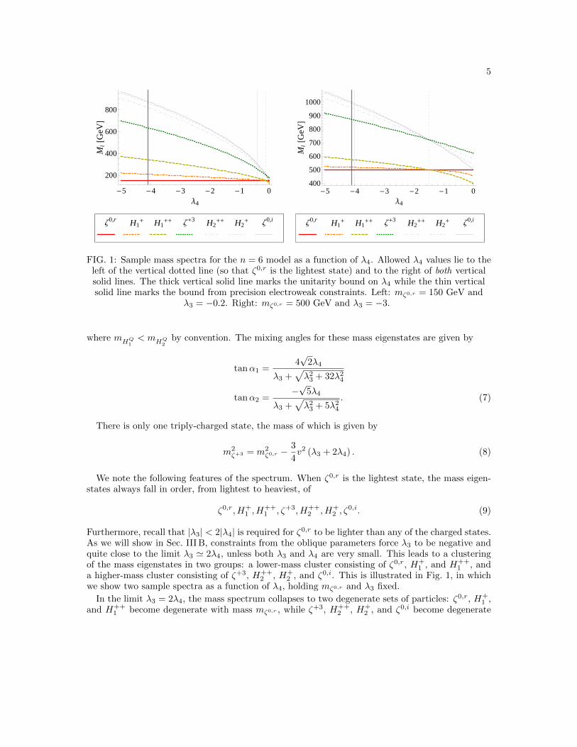
FIG. 1: Sample mass spectra for the n = 6 model as a function of λ4. Allowed λ4 values lie to theleft of the vertical dotted line (so that ζ0,r is the lightest state) and to the right of both verticalsolid lines. The thick vertical solid line marks the unitarity bound on λ4 while the thin verticalsolid line marks the bound from precision electroweak constraints. Left: mζ0,r = 150 GeV and
λ3 = −0.2. Right: mζ0,r = 500 GeV and λ3 = −3.
where mHQ1< mHQ
2by convention. The mixing angles for these mass eigenstates are given by
tanα1 =4√
2λ4
λ3 +√λ23 + 32λ24
tanα2 =−√
5λ4
λ3 +√λ23 + 5λ24
. (7)
There is only one triply-charged state, the mass of which is given by
m2ζ+3 = m2
ζ0,r −3
4v2 (λ3 + 2λ4) . (8)
We note the following features of the spectrum. When ζ0,r is the lightest state, the mass eigen-states always fall in order, from lightest to heaviest, of
ζ0,r, H+1 , H
++1 , ζ+3, H++
2 , H+2 , ζ
0,i. (9)
Furthermore, recall that |λ3| < 2|λ4| is required for ζ0,r to be lighter than any of the charged states.As we will show in Sec. III B, constraints from the oblique parameters force λ3 to be negative andquite close to the limit λ3 ' 2λ4, unless both λ3 and λ4 are very small. This leads to a clusteringof the mass eigenstates in two groups: a lower-mass cluster consisting of ζ0,r, H+
1 , and H++1 , and
a higher-mass cluster consisting of ζ+3, H++2 , H+
2 , and ζ0,i. This is illustrated in Fig. 1, in whichwe show two sample spectra as a function of λ4, holding mζ0,r and λ3 fixed.
In the limit λ3 = 2λ4, the mass spectrum collapses to two degenerate sets of particles: ζ0,r, H+1 ,
and H++1 become degenerate with mass mζ0,r , while ζ+3, H++
2 , H+2 , and ζ0,i become degenerate
6
with with mass mζ0,i =√m2ζ0,r − 3v2λ4. In this limit, the composition of the mixed states in the
n = 6 model becomes
H+1 =
√1
3ζ+1 −
√2
3ζ−1∗, H+
2 =
√2
3ζ+1 +
√1
3ζ−1∗
H++1 =
√1
6ζ+2 +
√5
6ζ−2∗, H++
2 = −√
5
6ζ+2 +
√1
6ζ−2∗. (10)
In particular, all transitions among the mass eigenstates mediated by W± or Z emission proceedwith roughly comparable coupling strength.
B. n = 8 model
The mass of the real part of ζ0 in the n = 8 model is given by
m2ζ0,r = M2 +
1
2v2[λ2 +
1
4λ3 − 4λ4
]≡M2 +
1
2v2Λ8, (11)
where Λ8 is defined as the quantity in brackets above. The mass of the imaginary part of ζ0 is then
m2ζ0,i = m2
ζ0,r + 4v2λ4 . (12)
Since we have chosen ζ0,r as the lightest member, we are forced to take λ4 > 0.The singly-, doubly-, and triply-charged states have masses
m2H+
1,2= m2
ζ0,r +1
4v2(
8λ4 ∓√λ23 + 60λ24
)m2H++
1,2= m2
ζ0,r +1
2v2(
4λ4 ∓√λ23 + 12λ24
)m2H+3
1,2= m2
ζ0,r +1
4v2(
8λ4 ∓√
9λ23 + 28λ24
), (13)
where again mHQ1< mHQ
2by convention. The mixing angles for these mass eigenstates are given
by
tanα1 =−2√
15λ4
λ3 +√λ23 + 60λ24
tanα2 =2√
3λ4
λ3 +√λ23 + 12λ24
tanα3 =−2√
7λ4
3λ3 +√
9λ23 + 28λ24. (14)
There is only one quadruply-charged state, the mass of which is given by
m2ζ+4 = m2
ζ0,r − v2 (λ3 − 2λ4) . (15)
7
When ζ0,r is the lightest state, the mass eigenstates always fall in order, from lightest to heaviest,of
ζ0,r, H+1 , H
++1 , H+3
1 , ζ+4, H+32 , H++
2 , H+2 , ζ
0,i. (16)
Constraints from the oblique parameters will again force λ3 to be negative and quite close to thelimit λ3 ' −2λ4 (with |λ3| < 2|λ4|). In this limit, the mass spectrum again collapses to twodegenerate sets of particles: ζ0,r, H+
1 , H++1 , and H+3
1 become degenerate with mass mζ0,r , while
ζ+4, H+32 , H++
2 , H+2 , and ζ0,i become degenerate with mass mζ0,i =
√m2ζ0,r + 4v2λ4. In this limit,
the composition of the mixed states in the n = 8 model becomes
H+1 =
√3
8ζ+1 −
√5
8ζ−1∗, H+
2 =
√5
8ζ+1 +
√3
8ζ−1∗
H++1 =
√1
4ζ+2 +
√3
4ζ−2∗, H++
2 = −√
3
4ζ+2 +
√1
4ζ−2∗
H+31 =
√1
8ζ+3 −
√7
8ζ−3∗, H+3
2 =
√7
8ζ+3 +
√1
8ζ−3∗. (17)
Again, all transitions among the mass eigenstates mediated by W± or Z emission proceed withroughly comparable coupling strength.
III. CONSTRAINTS ON COUPLINGS AND MASSES
In this section we determine the constraints on the model parameters from perturbative unitarity,from the oblique parameters S, T , and U , and from the contributions of the new charged scalarsto the loop-induced decays of the SM Higgs boson, h→ γγ and h→ Zγ.
Throughout this section, we show numerical results for the real neutral scalar in the mass rangemζ0,r = 80–500 GeV. We expect that scalars lighter than 80 GeV will be strongly constrainedby searches at the CERN Large Electron-Positron (LEP) collider. We leave the analysis of LEPconstraints and CERN Large Hadron Collider (LHC) discovery prospects to future work.
A. Unitarity constraints on scalar quartic couplings
The scalar quartic couplings λ2, λ3 and λ4 given in Eq. (1) can be bounded by requiring pertur-bative unitarity of the zeroth partial wave scattering amplitudes. The partial wave amplitudes arerelated to scattering matrix elements according to
M = 16π∑J
(2J + 1)aJPJ(cos θ), (18)
where J is the orbital angular momentum of the final state and PJ(cos θ) is the correspondingLegendre polynomial. Perturbative unitarity of the zeroth partial wave amplitude dictates thetree-level constraint,
|Re a0| ≤1
2. (19)
8
We perform a coupled-channel analysis for processes SS → SS and SS → V V , where SS denotesany pair of scalars contained in Φ or Z and V V denotes any pair of transversely-polarized elec-troweak gauge bosons. We include the SS → V V channels only for scalars contained in Z, whoseamplitudes are enhanced by the large value of n.4 We work in the high-energy limit and treat theGoldstone bosons as physical particles in place of the longitudinal components of the electroweakgauge bosons. For simplicity, we further neglect contributions from the quartic coupling λ1, whichis known to be small now that the SM-like Higgs boson mass has been measured, and from quarticcouplings involving four Z fields. We find numerically that including such contributions leads totighter constraints on λ2, λ3, and λ4. As such, our bounds are conservative.
The scattering amplitudes are conveniently classified according to the total isospin and totalhypercharge of the initial and final two-particle states. The relevant amplitudes for the isospin-zero, hypercharge-zero channels are [14]
a0([ζ∗ζ]0 → [φ∗φ]0) = −√n
8√
2πλ2,
a0([ζ∗ζ]0 → [WW ]0) =g2
16π
(n2 − 1)√n
2√
3,
a0([ζ∗ζ]0 → [BB]0) =g2
16π
s2Wc2W
Y 2√n
2, (20)
where the ζ∗ζ → WW,BB amplitudes include both of the contributing transverse gauge bosonpolarization combinations [12]. Here g is the SU(2)L gauge coupling and sW , cW ≡ sin θW , cos θWare the sine and cosine of the weak mixing angle, and Y = 1 for our models. We define the followingnormalized isospin-zero, hypercharge-zero field combinations,
[φ∗φ]0 =1√2
(φ+φ− + φ0∗φ0),
[ζ∗ζ]0 =1√n
∑Q
ζQ∗ζQ,
[WW ]0 =1√3
(√2W+W− +
(W 3W 3
√2
)),
[BB]0 = BB/√
2, (21)
where the sum over Q runs over the n isospin eigenstates in Z as shown in Eq. (2). The relevantamplitudes for the isospin-one, hypercharge-zero channels are [14]
a0([ζ∗ζ]1 → [φ∗φ]1) = −√n(n2 − 1)
32√
6πλ3,
a0([ζ∗ζ]1 → [WB]1) =g2
16π
sWcW
Y√n(n2 − 1)√
6, (22)
where again the ζ∗ζ → WB amplitude includes both of the contributing transverse gauge bosonpolarization combinations [12]. Here we used the following normalized isospin-one, hypercharge-zero
4 This is the phenomenon that ultimately puts an upper limit on n [12].
9
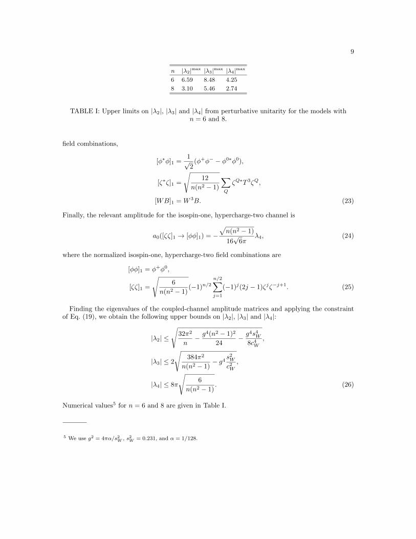
n |λ2|max |λ3|max |λ4|max
6 6.59 8.48 4.25
8 3.10 5.46 2.74
TABLE I: Upper limits on |λ2|, |λ3| and |λ4| from perturbative unitarity for the models withn = 6 and 8.
field combinations,
[φ∗φ]1 =1√2
(φ+φ− − φ0∗φ0),
[ζ∗ζ]1 =
√12
n(n2 − 1)
∑Q
ζQ∗T 3ζQ,
[WB]1 = W 3B. (23)
Finally, the relevant amplitude for the isospin-one, hypercharge-two channel is
a0([ζζ]1 → [φφ]1) = −√n(n2 − 1)
16√
6πλ4, (24)
where the normalized isospin-one, hypercharge-two field combinations are
[φφ]1 = φ+φ0,
[ζζ]1 =
√6
n(n2 − 1)(−1)n/2
n/2∑j=1
(−1)j(2j − 1)ζjζ−j+1. (25)
Finding the eigenvalues of the coupled-channel amplitude matrices and applying the constraintof Eq. (19), we obtain the following upper bounds on |λ2|, |λ3| and |λ4|:
|λ2| ≤
√32π2
n− g4(n2 − 1)2
24−g4s4W8c4W
,
|λ3| ≤ 2
√384π2
n(n2 − 1)− g4
s2Wc2W
,
|λ4| ≤ 8π
√6
n(n2 − 1). (26)
Numerical values5 for n = 6 and 8 are given in Table I.
5 We use g2 = 4πα/s2W , s2W = 0.231, and α = 1/128.
10
B. Constraints from the oblique parameters S, T and U
Further constraints can be obtained from experimental measurements of the electroweak obliqueparameters S, T and U [15]. These parameters probe new physics that can appear in loops in theelectroweak gauge boson self-energies. They were previously calculated for a large scalar multipletwith arbitrary isospin and hypercharge in the case of a global U(1) symmetry in Ref. [16]. Werecomputed the contributions of a large scalar multiplet to S, T and U for the global Z2-preservingcase, in which the mass eigenstates do not always correspond to isospin eigenstates. We checkedthat our results reduce to the U(1)-preserving limit when λ4 → 0.
For the S parameter we find,
S =s2W c
2W
π
∑i,j
(|CijZ |2 −
c2W − s2WsW cW
CijZC∗ijγ − |Cijγ |2
)f1(mi,mj), (27)
where the couplings CijV involving scalars i, j and vector boson V are defined with an over-all factor of e removed (see Appendix B 2). The sums over states i and j run over ij =ζ0,rζ0,i, H+Q
k H−Ql , ζn/2ζ−n/2
, where kl = 11, 12, 21, 22 and Q > 0. The dimensionless func-
tion f1(m1,m2) is defined as
f1(m1,m2) = f1(m2,m1) =
∫ 1
0
dxx(1− x) log[xm2
1 + (1− x)m22
], (28)
=
5(m6
2−m61)+27(m4
1m22−m
21m
42)+12(m6
1−3m41m
22) log(m1)+12(3m2
1m42−m
62) log(m2)
36(m21−m2
2)3 for m1 6= m2 ,
16 logm2
1 for m1 = m2 .(29)
For the T parameter we find,
T =1
4πM2Z
[∑r
Sr
(Crr∗W+W−
cW− Crr∗ZZ
)f2(mr,mr)
−2∑s,t
|CstW+ |2
cWf2(ms,mt) + 2
∑i,j
|CijZ |2f2(mi,mj)
, (30)
where the couplings Crr∗XY involving scalars rr∗ and vector bosons X, Y are defined withan overall factor of e2 removed (see Appendix B 2). The sum over states r runs over r =ζ0,r, ζ0,i, HQ
k , ζn/2
, with Q > 0 and k = 1, 2. For these couplings, Sr is a symmetry factor
given by Sr = 1/2 for r = ζ0,r or ζ0,i and Sr = 1 otherwise. The sums over states s and t run
over st =ζ0,rH−k , ζ
0,iH−k , H+Qk H−Q−1l , ζn/2H
−n/2−1k
, where again kl = 11, 12, 21, 22 and Q > 0.
The sums over states i and j run over the same set of states given below Eq. (27). The functionf2(m1,m2) has dimensions of mass-squared and is defined as
f2(m1,m2) = f2(m2,m1) =
∫ 1
0
dx(xm2
1 + (1− x)m22
)log[xm2
1 + (1− x)m22
]=
− 1
4 (m21 +m2
2) + 1m2
1−m22
[m4
1 logm1 −m42 logm2
]for m1 6= m2 ,
m21 logm2
1 for m1 = m2.(31)
11
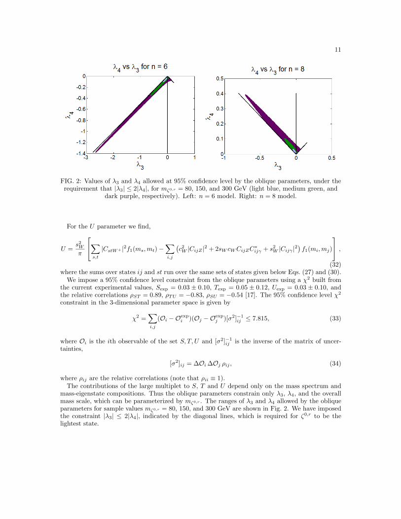
FIG. 2: Values of λ3 and λ4 allowed at 95% confidence level by the oblique parameters, under therequirement that |λ3| ≤ 2|λ4|, for mζ0,r = 80, 150, and 300 GeV (light blue, medium green, and
dark purple, respectively). Left: n = 6 model. Right: n = 8 model.
For the U parameter we find,
U =s2Wπ
∑s,t
|CstW+ |2f1(ms,mt)−∑i,j
(c2W |CijZ |2 + 2sW cWCijZC
∗ijγ + s2W |Cijγ |2
)f1(mi,mj)
,(32)
where the sums over states ij and st run over the same sets of states given below Eqs. (27) and (30).We impose a 95% confidence level constraint from the oblique parameters using a χ2 built from
the current experimental values, Sexp = 0.03 ± 0.10, Texp = 0.05 ± 0.12, Uexp = 0.03 ± 0.10, andthe relative correlations ρST = 0.89, ρTU = −0.83, ρSU = −0.54 [17]. The 95% confidence level χ2
constraint in the 3-dimensional parameter space is given by
χ2 =∑i,j
(Oi −Oexpi )(Oj −Oexp
j )[σ2]−1ij ≤ 7.815, (33)
where Oi is the ith observable of the set S, T, U and [σ2]−1ij is the inverse of the matrix of uncer-tainties,
[σ2]ij = ∆Oi ∆Oj ρij , (34)
where ρij are the relative correlations (note that ρii ≡ 1).The contributions of the large multiplet to S, T and U depend only on the mass spectrum and
mass-eigenstate compositions. Thus the oblique parameters constrain only λ3, λ4, and the overallmass scale, which can be parameterized by mζ0,r . The ranges of λ3 and λ4 allowed by the obliqueparameters for sample values mζ0,r = 80, 150, and 300 GeV are shown in Fig. 2. We have imposedthe constraint |λ3| ≤ 2|λ4|, indicated by the diagonal lines, which is required for ζ0,r to be thelightest state.
12
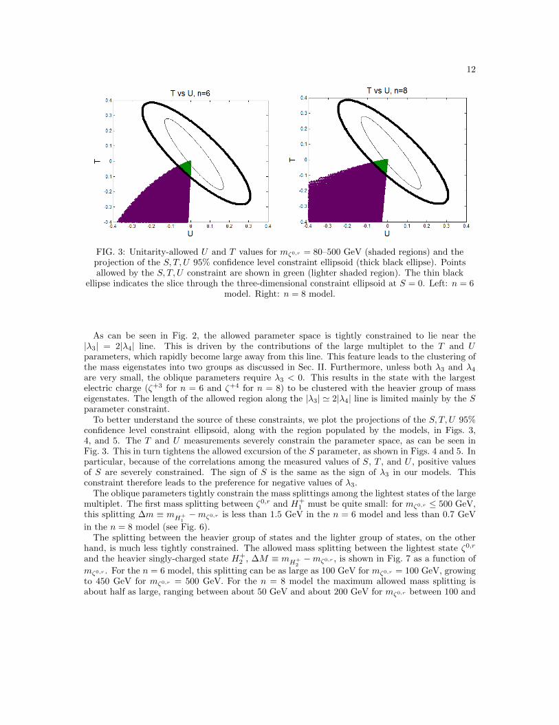
FIG. 3: Unitarity-allowed U and T values for mζ0,r = 80–500 GeV (shaded regions) and theprojection of the S, T, U 95% confidence level constraint ellipsoid (thick black ellipse). Pointsallowed by the S, T, U constraint are shown in green (lighter shaded region). The thin black
ellipse indicates the slice through the three-dimensional constraint ellipsoid at S = 0. Left: n = 6model. Right: n = 8 model.
As can be seen in Fig. 2, the allowed parameter space is tightly constrained to lie near the|λ3| = 2|λ4| line. This is driven by the contributions of the large multiplet to the T and Uparameters, which rapidly become large away from this line. This feature leads to the clustering ofthe mass eigenstates into two groups as discussed in Sec. II. Furthermore, unless both λ3 and λ4are very small, the oblique parameters require λ3 < 0. This results in the state with the largestelectric charge (ζ+3 for n = 6 and ζ+4 for n = 8) to be clustered with the heavier group of masseigenstates. The length of the allowed region along the |λ3| ' 2|λ4| line is limited mainly by the Sparameter constraint.
To better understand the source of these constraints, we plot the projections of the S, T, U 95%confidence level constraint ellipsoid, along with the region populated by the models, in Figs. 3,4, and 5. The T and U measurements severely constrain the parameter space, as can be seen inFig. 3. This in turn tightens the allowed excursion of the S parameter, as shown in Figs. 4 and 5. Inparticular, because of the correlations among the measured values of S, T , and U , positive valuesof S are severely constrained. The sign of S is the same as the sign of λ3 in our models. Thisconstraint therefore leads to the preference for negative values of λ3.
The oblique parameters tightly constrain the mass splittings among the lightest states of the largemultiplet. The first mass splitting between ζ0,r and H+
1 must be quite small: for mζ0,r ≤ 500 GeV,this splitting ∆m ≡ mH+
1−mζ0,r is less than 1.5 GeV in the n = 6 model and less than 0.7 GeV
in the n = 8 model (see Fig. 6).The splitting between the heavier group of states and the lighter group of states, on the other
hand, is much less tightly constrained. The allowed mass splitting between the lightest state ζ0,r
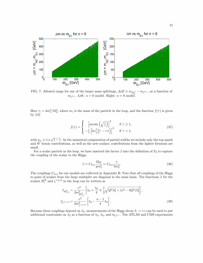
and the heavier singly-charged state H+2 , ∆M ≡ mH+
2−mζ0,r , is shown in Fig. 7 as a function of
mζ0,r . For the n = 6 model, this splitting can be as large as 100 GeV for mζ0,r = 100 GeV, growingto 450 GeV for mζ0,r = 500 GeV. For the n = 8 model the maximum allowed mass splitting isabout half as large, ranging between about 50 GeV and about 200 GeV for mζ0,r between 100 and
13
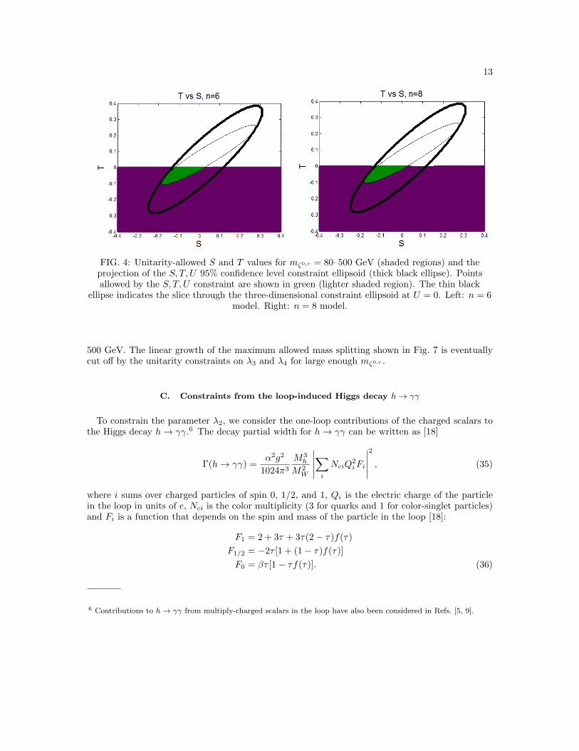
FIG. 4: Unitarity-allowed S and T values for mζ0,r = 80–500 GeV (shaded regions) and theprojection of the S, T, U 95% confidence level constraint ellipsoid (thick black ellipse). Pointsallowed by the S, T, U constraint are shown in green (lighter shaded region). The thin black
ellipse indicates the slice through the three-dimensional constraint ellipsoid at U = 0. Left: n = 6model. Right: n = 8 model.
500 GeV. The linear growth of the maximum allowed mass splitting shown in Fig. 7 is eventuallycut off by the unitarity constraints on λ3 and λ4 for large enough mζ0,r .
C. Constraints from the loop-induced Higgs decay h→ γγ
To constrain the parameter λ2, we consider the one-loop contributions of the charged scalars tothe Higgs decay h→ γγ.6 The decay partial width for h→ γγ can be written as [18]
Γ(h→ γγ) =α2g2
1024π3
M3h
M2W
∣∣∣∣∣∑i
NciQ2iFi
∣∣∣∣∣2
, (35)
where i sums over charged particles of spin 0, 1/2, and 1, Qi is the electric charge of the particlein the loop in units of e, Nci is the color multiplicity (3 for quarks and 1 for color-singlet particles)and Fi is a function that depends on the spin and mass of the particle in the loop [18]:
F1 = 2 + 3τ + 3τ(2− τ)f(τ)
F1/2 = −2τ [1 + (1− τ)f(τ)]
F0 = βτ [1− τf(τ)]. (36)
6 Contributions to h→ γγ from multiply-charged scalars in the loop have also been considered in Refs. [5, 9].

14
FIG. 5: Unitarity-allowed S and U values for mζ0,r = 80–500 GeV (shaded regions) and theprojection of the S, T, U 95% confidence level constraint ellipsoid (thick black ellipse). Pointsallowed by the S, T, U constraint are shown in green (lighter shaded region). The thin black
ellipse indicates the slice through the three-dimensional constraint ellipsoid at T = 0. Scatter inthe plot is due to the numerical scan. Left: n = 6 model. Right: n = 8 model.
FIG. 6: Allowed range for the first mass splitting ∆m ≡ mH+1−mζ0,r as a function of mζ0,r . Left:
n = 6 model. Right: n = 8 model.
15
FIG. 7: Allowed range for one of the larger mass splittings, ∆M ≡ mH+2−mζ0,r , as a function of
mζ0,r . Left: n = 6 model. Right: n = 8 model.
Here τi = 4m2i /M
2h , where mi is the mass of the particle in the loop, and the function f(τ) is given
by [18]
f(τ) =
[arcsin
(√1τ
)]2if τ ≥ 1,
− 14
[ln(η+η−− i π
)]2if τ < 1,
(37)
with η± ≡ 1±√
1− τ . In the numerical computation of partial widths we include only the top quarkand W boson contributions, as well as the new scalars; contributions from the lighter fermions aresmall.
For a scalar particle in the loop, we have inserted the factor β into the definition of F0 to capturethe coupling of the scalar to the Higgs,
β = ChssMW
gm2s
= Chssv
2m2s
. (38)
The couplings Chss for our models are collected in Appendix B. Note that all couplings of the Higgsto pairs of scalars from the large multiplet are diagonal in the mass basis. The functions β for the
scalars HQi and ζ+n/2 in the loop can be written as
βHQ1,2
=v2
2m2HQ
1,2
[λ2 +
λ34∓ 1
2
√Q2λ23 + (n2 − 4Q2)λ24
],
βζ+n/2 =v2
2m2ζ+n/2
[λ2 −
n− 1
4λ3
]. (39)
Because these couplings depend on λ2, measurements of the Higgs decay h→ γγ can be used to putadditional constraints on λ2 as a function of λ3, λ4, and mζ0,r . The ATLAS and CMS experiments
16
Observable ATLAS CMS
µγγ 1.65+0.32−0.30 [19] 0.78
+0.28−0.26 [20]
µZγ < 18.2 [21] < 10 [22]
TABLE II: Current measurements of the signal strengths for h→ γγ and h→ Zγ relative to theSM predictions. For h→ Zγ we quote the 95% confidence level upper bounds for Mh = 125 GeV.
have measured the Higgs signal strength µγγ in the γγ final state, defined relative to the SMprediction. Because Higgs production rates are not modified in our models, and because the onlysignificant effect of the new scalars on Higgs decays is through modification of the partial widthsof the rare loop-induced processes h→ γγ and h→ Zγ, we have to a very good approximation
µγγ ' Rγγ ≡Γ(h→ γγ)
ΓSM(h→ γγ), (40)
and an analogous expression for RZγ . The measured values of this rate from ATLAS and CMS aresummarized in Table II.
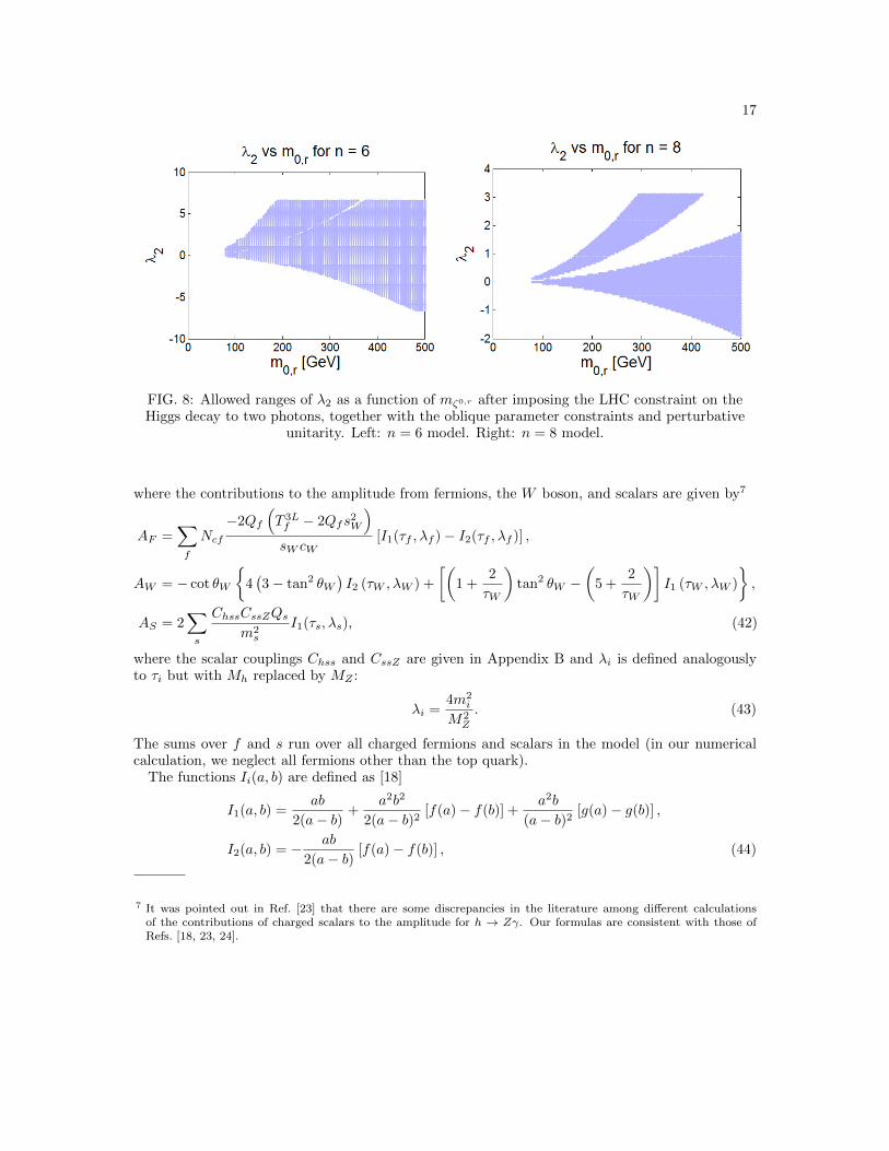
We find the allowed range of λ2 as a function of mζ0,r by scanning over the values of λ3 andλ4 allowed by the oblique parameter constraints and perturbative unitarity. We accept points forwhich Rγγ falls within the 2σ range for µγγ of either the ATLAS or CMS measurement. Resultsare shown in Fig. 8. Note that the constraint from perturbative unitarity, |λ2| ≤ 6.59 (3.10) forn = 6 (8), is visible in the plots. The upper branch of allowed λ2 values, clearly visible in the rightpanel of Fig. 8 for n = 8, corresponds to a sign flip of the total h → γγ amplitude relative to theSM prediction. This is separated from the rest of the points due to the lower bound on µγγ . Thesame feature is present in the n = 6 case, though it is less clearly visible in Fig. 8 due to the widerallowed ranges of λ3 and λ4.
The application of the h → γγ constraint does not significantly restrict the range of λ3 or λ4beyond the constraints already obtained from the oblique parameters and perturbative unitarity.
D. Predictions for h→ Zγ
The charged scalars in our models also contribute to the loop-induced decay h→ Zγ. The decaypartial width for this process can be written as (see, e.g., Ref. [18])
Γ(h→ Zγ) =α2
512π3
∣∣∣∣2v (AF +AW ) +AS
∣∣∣∣2M3h
[1− M2
Z
M2h
]3, (41)
17
FIG. 8: Allowed ranges of λ2 as a function of mζ0,r after imposing the LHC constraint on theHiggs decay to two photons, together with the oblique parameter constraints and perturbative
unitarity. Left: n = 6 model. Right: n = 8 model.
where the contributions to the amplitude from fermions, the W boson, and scalars are given by7
AF =∑f
Ncf−2Qf
(T 3Lf − 2Qfs
2W
)sW cW
[I1(τf , λf )− I2(τf , λf )] ,
AW = − cot θW
4(3− tan2 θW
)I2 (τW , λW ) +
[(1 +
2
τW
)tan2 θW −
(5 +
2
τW
)]I1 (τW , λW )
,
AS = 2∑s
ChssCssZQsm2s
I1(τs, λs), (42)
where the scalar couplings Chss and CssZ are given in Appendix B and λi is defined analogouslyto τi but with Mh replaced by MZ :
λi =4m2
i
M2Z
. (43)
The sums over f and s run over all charged fermions and scalars in the model (in our numericalcalculation, we neglect all fermions other than the top quark).
The functions Ii(a, b) are defined as [18]
I1(a, b) =ab
2(a− b)+
a2b2
2(a− b)2[f(a)− f(b)] +
a2b
(a− b)2[g(a)− g(b)] ,
I2(a, b) = − ab
2(a− b)[f(a)− f(b)] , (44)
7 It was pointed out in Ref. [23] that there are some discrepancies in the literature among different calculationsof the contributions of charged scalars to the amplitude for h → Zγ. Our formulas are consistent with those ofRefs. [18, 23, 24].
18
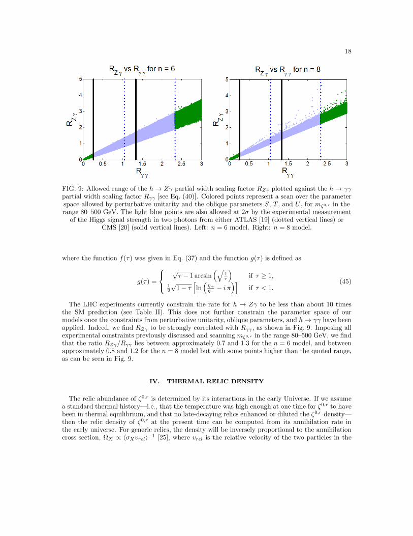
FIG. 9: Allowed range of the h→ Zγ partial width scaling factor RZγ plotted against the h→ γγpartial width scaling factor Rγγ [see Eq. (40)]. Colored points represent a scan over the parameterspace allowed by perturbative unitarity and the oblique parameters S, T , and U , for mζ0,r in therange 80–500 GeV. The light blue points are also allowed at 2σ by the experimental measurement
of the Higgs signal strength in two photons from either ATLAS [19] (dotted vertical lines) orCMS [20] (solid vertical lines). Left: n = 6 model. Right: n = 8 model.
where the function f(τ) was given in Eq. (37) and the function g(τ) is defined as
g(τ) =
√τ − 1 arcsin
(√1τ
)if τ ≥ 1,
12
√1− τ
[ln(η+η−− i π
)]if τ < 1.
(45)
The LHC experiments currently constrain the rate for h → Zγ to be less than about 10 timesthe SM prediction (see Table II). This does not further constrain the parameter space of ourmodels once the constraints from perturbative unitarity, oblique parameters, and h→ γγ have beenapplied. Indeed, we find RZγ to be strongly correlated with Rγγ , as shown in Fig. 9. Imposing allexperimental constraints previously discussed and scanning mζ0,r in the range 80–500 GeV, we findthat the ratio RZγ/Rγγ lies between approximately 0.7 and 1.3 for the n = 6 model, and betweenapproximately 0.8 and 1.2 for the n = 8 model but with some points higher than the quoted range,as can be seen in Fig. 9.
IV. THERMAL RELIC DENSITY
The relic abundance of ζ0,r is determined by its interactions in the early Universe. If we assumea standard thermal history—i.e., that the temperature was high enough at one time for ζ0,r to havebeen in thermal equilibrium, and that no late-decaying relics enhanced or diluted the ζ0,r density—then the relic density of ζ0,r at the present time can be computed from its annihilation rate inthe early universe. For generic relics, the density will be inversely proportional to the annihilationcross-section, ΩX ∝ 〈σXvrel〉−1 [25], where vrel is the relative velocity of the two particles in the
19
annihilation collision and the brackets indicate an average over this velocity distribution at thetime of freeze-out. Such an average is numerically necessary only if the annihilation cross sectionvanishes in the vrel → 0 limit. Because of this simple relationship, we can determine the fractionof the total dark matter that is made up by ζ0,r using the formula
Ωζ0,r
ΩDM=
〈σvrel〉std〈σvrel(ζ0,rζ0,r → any)〉
, (46)
where ΩDM is the current total dark matter relic abundance and 〈σvrel〉std is the “standard” anni-hilation cross section required to obtain this total dark matter relic abundance, for which we use〈σvrel〉std = 3× 10⁻²⁶ cm3/s [25].
A. Annihilations to two-body final states
The ζ0,r is a self-annihilating particle which interacts with the SM via gauge or Higgs bosonexchange. As such, the final states for the annihilation of two ζ0,r particles include W+W−, ZZ,hh, and ff (via s-channel Higgs exchange). We neglect co-annihilations with other scalars from theZ2-odd multiplet. We compute the annihilation cross sections in the zero-velocity limit. Becausethese cross sections are all nonzero in this limit, we do not need to average over the velocitydistribution.
The annihilation cross sections to two-body final states are given in the vrel → 0 limit by,
σvrel(ζ0,rζ0,r →W+W−) =
M4W
8πv4
√1−
M2W
m2ζ0,r
[A2W
m2ζ0,r
(3− 4
m2ζ0,r
M2W
+ 4m4ζ0,r
M4W
)
+2AWBW
(1− 3
m2ζ0,r
M2W
+ 2m4ζ0,r
M4W
)+B2
Wm2ζ0,r
(1−
m2ζ0,r
M2W
)2 ,
σvrel(ζ0,rζ0,r → ZZ) =
M4Z
16πv4
√1−
M2Z
m2ζ0,r
[A2Z
m2ζ0,r
(3− 4
m2ζ0,r
M2Z
+ 4m4ζ0,r
M4Z
)
+2AZBZ
(1− 3
m2ζ0,r
M2Z
+ 2m4ζ0,r
M4Z
)+B2
Zm2ζ0,r
(1−
m2ζ0,r
M2Z
)2 ,
σvrel(ζ0,rζ0,r → hh) =
Λ2n
64πm2ζ0,r
√1−
M2h
m2ζ0,r
[1 +
3M2h
4m2ζ0,r −M2
h
− 2v2Λn2m2
ζ0,r −M2h
]2,
σvrel(ζ0,rζ0,r → ff) =
Nc4π
[1−
m2f
m2ζ0,r
]3/2m2fΛ2
n
(4m2ζ0,r −M2
h)2, (47)
where n = 6, 8 is the size of the multiplet, Nc is the number of colors of the final-state fermions,and v ' 246 GeV is the usual Higgs vacuum expectation value. The coefficients used in the cross
20
section formulas for ζ0,rζ0,r →W+W− and ζ0,rζ0,r → ZZ are given by
AZ = 1 +Λnv
2
4m2ζ0,r −M2
h
(48)
BZ =4
M2Z −m2
ζ0,r −m2ζ0,i
(49)
AW =n2 − 2
2+
Λnv2
4m2ζ0,r −M2
h
, (50)
BW =
(n cosα1 −
√n2 − 4 sinα1
)2M2W −m2
ζ0,r −m2H+
1
+
(−n sinα1 −
√n2 − 4 cosα1
)2M2W −m2
ζ0,r −m2H+
2
. (51)
The combinations of couplings Λ6 and Λ8 were defined in Eqs. (4) and (11), respectively; they canboth be expressed by the formula
Λn = λ2 +1
4λ3 +
n
2(−1)n/2+1λ4. (52)
We note that when mζ0,r MW ,MZ , the annihilation cross sections for ζ0,rζ0,r → W+W−
and ZZ go like 1/m2ζ0,r . In this limit, the new scalars become increasingly degenerate due to the
constraints on the size of |λ3| and |λ4|; the values of AW,Z and BW,Z are then related in such a wayas to allow a cancellation of the m2
ζ0,r/M2W,Z and m4
ζ0,r/M4W,Z terms in the square brackets, which
would otherwise make the cross section grow with increasing mζ0,r . This cancellation providesa nice cross-check of the matrix element calculation. We also checked our analytic results usingCalcHEP [26].
B. Numerical results
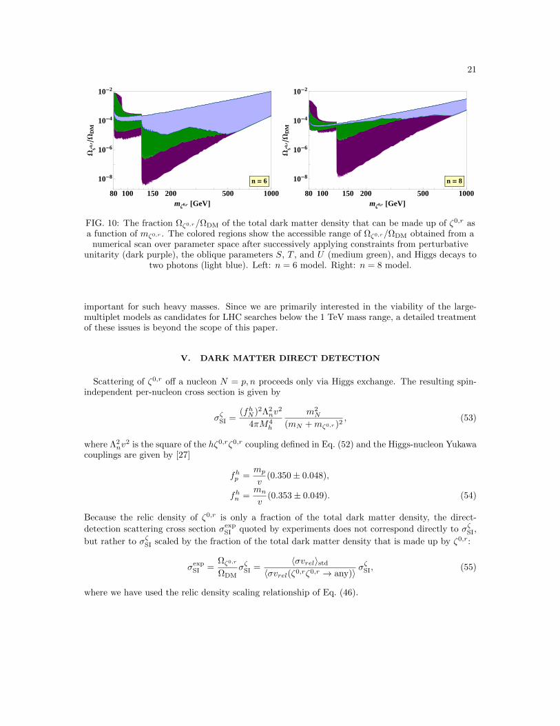
In Fig. 10 we show the fraction of the total dark matter density that can be made up of ζ0,r,computed using Eq. (46) including all kinematically accessible two-body final states, as a functionof mζ0,r for the models with n = 6 and 8. We scan over λ2, λ3, and λ4, applying in succession theconstraints from perturbative unitarity (dark purple regions), the oblique parameters S, T , and U(medium green regions), and Higgs decays to two photons (light blue regions).
The possibility of very small relic densities that opens up when mζ0,r > 125 GeV is due to thecrossing of the the kinematic threshold for ζ0,rζ0,r → hh. However, imposition of the obliqueparameter constraints (medium green) and particularly the h→ γγ constraint (light blue) severelylimits the allowed strength Λn of the h(h)ζ0,rζ0,r couplings, leading to a more tightly constrainedrelic density. For ζ0,r masses above about 500 GeV in the n = 6 model (800 GeV in the n = 8model) the constraints on λ2, λ3, and λ4 come only from perturbative unitarity.
We find that, for allowed parameter choices and mζ0,r . 1 TeV, the thermal relic abundance ofζ0,r can account for at most 1% of the dark matter. In particular, the two models that we studyare consistent with the observed dark matter relic abundance and thus viable extensions of the SM,assuming that most of the dark matter is made up of some other candidate particle.
Extending our calculation to higher masses, we find that ζ0,r could account for all the darkmatter for masses of 10–33 TeV for the n = 6 model, or 18–30 TeV for the n = 8 model. However,we have not included effects from co-annihilations or Sommerfeld enhancement which may become
21
80 100 150 200 500 1000
10-8
10-6
10-4
10-2
mΖ0,r @GeVD
WΖ
0,r W
DM
n = 6
80 100 150 200 500 1000
10-8
10-6
10-4
10-2
mΖ0,r @GeVD
WΖ
0,r W
DM
n = 8
FIG. 10: The fraction Ωζ0,r/ΩDM of the total dark matter density that can be made up of ζ0,r asa function of mζ0,r . The colored regions show the accessible range of Ωζ0,r/ΩDM obtained from a
numerical scan over parameter space after successively applying constraints from perturbativeunitarity (dark purple), the oblique parameters S, T , and U (medium green), and Higgs decays to
two photons (light blue). Left: n = 6 model. Right: n = 8 model.
important for such heavy masses. Since we are primarily interested in the viability of the large-multiplet models as candidates for LHC searches below the 1 TeV mass range, a detailed treatmentof these issues is beyond the scope of this paper.
V. DARK MATTER DIRECT DETECTION
Scattering of ζ0,r off a nucleon N = p, n proceeds only via Higgs exchange. The resulting spin-independent per-nucleon cross section is given by
σζSI =(fhN )2Λ2
nv2
4πM4h
m2N
(mN +mζ0,r )2, (53)
where Λ2nv
2 is the square of the hζ0,rζ0,r coupling defined in Eq. (52) and the Higgs-nucleon Yukawacouplings are given by [27]
fhp =mp
v(0.350± 0.048),
fhn =mn
v(0.353± 0.049). (54)
Because the relic density of ζ0,r is only a fraction of the total dark matter density, the direct-
detection scattering cross section σexpSI quoted by experiments does not correspond directly to σζSI,
but rather to σζSI scaled by the fraction of the total dark matter density that is made up by ζ0,r:
σexpSI =
Ωζ0,r
ΩDMσζSI =
〈σvrel〉std〈σvrel(ζ0,rζ0,r → any)〉
σζSI, (55)
where we have used the relic density scaling relationship of Eq. (46).
22
80 100 150 200 500 100010-47
10-46
10-45
10-44
10-43
mΖ0,r @GeVD
Σex
pN
@cm
2 D
LUX H2013L
XENON1T
LUX
DEAP-3600
n = 6
80 100 150 200 500 100010-47
10-46
10-45
10-44
10-43
mΖ0,r @GeVD
Σex
pN
@cm
2 D
LUX H2013L
XENON1T
LUX
DEAP-3600
n = 8
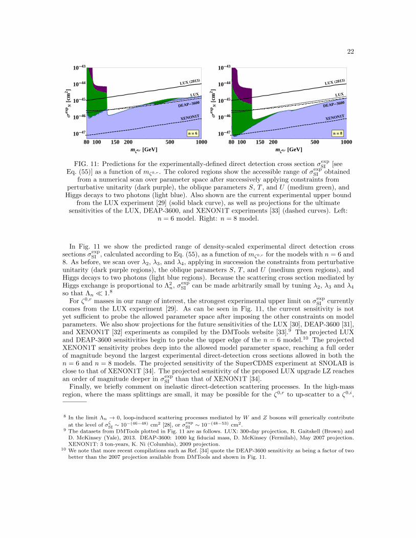
FIG. 11: Predictions for the experimentally-defined direct detection cross section σexpSI [see
Eq. (55)] as a function of mζ0,r . The colored regions show the accessible range of σexpSI obtained
from a numerical scan over parameter space after successively applying constraints fromperturbative unitarity (dark purple), the oblique parameters S, T , and U (medium green), and
Higgs decays to two photons (light blue). Also shown are the current experimental upper boundfrom the LUX experiment [29] (solid black curve), as well as projections for the ultimate
sensitivities of the LUX, DEAP-3600, and XENON1T experiments [33] (dashed curves). Left:n = 6 model. Right: n = 8 model.
In Fig. 11 we show the predicted range of density-scaled experimental direct detection crosssections σexp
SI , calculated according to Eq. (55), as a function of mζ0,r for the models with n = 6 and8. As before, we scan over λ2, λ3, and λ4, applying in succession the constraints from perturbativeunitarity (dark purple regions), the oblique parameters S, T , and U (medium green regions), andHiggs decays to two photons (light blue regions). Because the scattering cross section mediated byHiggs exchange is proportional to Λ2
n, σexpSI can be made arbitrarily small by tuning λ2, λ3 and λ4
so that Λn 1.8
For ζ0,r masses in our range of interest, the strongest experimental upper limit on σexpSI currently
comes from the LUX experiment [29]. As can be seen in Fig. 11, the current sensitivity is notyet sufficient to probe the allowed parameter space after imposing the other constraints on modelparameters. We also show projections for the future sensitivities of the LUX [30], DEAP-3600 [31],and XENON1T [32] experiments as compiled by the DMTools website [33].9 The projected LUXand DEAP-3600 sensitivities begin to probe the upper edge of the n = 6 model.10 The projectedXENON1T sensitivity probes deep into the allowed model parameter space, reaching a full orderof magnitude beyond the largest experimental direct-detection cross sections allowed in both then = 6 and n = 8 models. The projected sensitivity of the SuperCDMS experiment at SNOLAB isclose to that of XENON1T [34]. The projected sensitivity of the proposed LUX upgrade LZ reachesan order of magnitude deeper in σexp
SI than that of XENON1T [34].Finally, we briefly comment on inelastic direct-detection scattering processes. In the high-mass
region, where the mass splittings are small, it may be possible for the ζ0,r to up-scatter to a ζ0,i,
8 In the limit Λn → 0, loop-induced scattering processes mediated by W and Z bosons will generically contribute
at the level of σζSI ∼ 10−(46−48) cm2 [28], or σexpSI ∼ 10−(48−53) cm2.
9 The datasets from DMTools plotted in Fig. 11 are as follows. LUX: 300-day projection, R. Gaitskell (Brown) andD. McKinsey (Yale), 2013. DEAP-3600: 1000 kg fiducial mass, D. McKinsey (Fermilab), May 2007 projection.XENON1T: 3 ton-years, K. Ni (Columbia), 2009 projection.
10 We note that more recent compilations such as Ref. [34] quote the DEAP-3600 sensitivity as being a factor of twobetter than the 2007 projection available from DMTools and shown in Fig. 11.
23
providing an alternative direct detection mechanism through Z-boson exchange. At the kinematicthreshold, the accessible mass splitting is given in terms of the ambient ζ0,r velocity vζ by
mζ0,i −mζ0,r ≤√m2A +m2
ζ0,r + 2mAmζ0,r
√1 + v2ζ − (mA +mζ0,r ), (56)
where mA is the mass of the scattering target. In our case, the current dark matter velocity isvζ ∼ 10−3c and the scattering target is a xenon nucleus with mA ≈ 124 GeV. For mζ0,r mA,Eq. (56) approaches a constant value, mζ0,i − mζ0,r . mAv
2ζ/2 ∼ 60 keV. In turn, this implies
that the mass splittings between the electrically-charged scalars and ζ0,r would be much less thanthe mass of an electron, forcing the electrically-charged scalars to be stable. We conclude that theabsence of heavy charged relics precludes the possibility of inelastic direct-detection scattering inour models.
VI. DISCUSSION AND CONCLUSIONS
In this paper we examined extensions of the SM scalar sector containing a single large multipletof SU(2)L in addition to the SM Higgs doublet. We focused on two models, one in which the largemultiplet has isospin T = 5/2 (n = 6) and hypercharge Y = 1 and the other with T = 7/2 (n = 8)and Y = 1. In these models the most general gauge-invariant renormalizable scalar potentialpreserves an accidental global Z2 symmetry that forces the lightest member of the large multipletto be stable.
We wrote down the scalar potential for each of the two models and worked out the spectrumof mass eigenstates and their couplings to SM gauge and Higgs bosons. We then determined theconstraints on the model parameters from perturbative unitarity, the oblique parameters S, T , andU , and SM Higgs decays to two photons. We computed the predictions for Higgs decays to Zγ,as well as the thermal relic abundance of the lightest member of the large multiplet and its crosssection in dark matter direct-detection experiments.
We found that both models are viable for a wide range of masses of the new scalars within thekinematic reach of the LHC. The mass splittings of the new scalars are constrained mainly by theoblique parameters, which force the mass eigenstates to be tightly clustered into two groups. Thesegroups can in turn be separated by tens to hundreds of GeV, depending on the mass of the lightestnew scalar. This feature of the spectrum will have interesting implications for the kinematics ofcollider events involving pair production and decay of the new scalars.
We finish by commenting on a few features of the models that may warrant further study.
• The masses of the new scalars are bounded from above by the requirement that their relicdensity not be larger than the observed dark matter density in the universe. This bound willlie in the several-to-tens of TeV range. An accurate determination of this bound will requirea more careful treatment of co-annihilations and Sommerfeld effects in the calculation of therelic density.
• The total cross section for production of pairs of the new scalars at the LHC via electroweakprocesses will be enhanced by the large multiplicity of scalar states and by their large weakcharges. The LHC reach for these particles may thus extend to higher masses than the reachfor other scalar extensions of the SM involving smaller representations of SU(2)L.
• Our models affect the running of the electroweak gauge couplings. In particular, the one-loop SU(2)L beta function coefficient becomes b2 = −19/6 + n(n2 − 1)/36, where α−12 (Λ) =
24
α−12 (MZ)− (b2/2π) log(Λ/MZ) and α2 ≡ g2/4π. In the n = 6 model, α2 remains perturbativeup to well beyond the Planck scale. In the n = 8 model, α2 becomes nonperturbative around1010 GeV. The n = 8 model can be saved by, e.g., lowering the Planck scale below 1010 GeVthrough the introduction of flat or warped extra dimensions. We note that ζ0,r in the n =8 model can decay via a dimension-8 Planck-suppressed operator; ζ0,r remains stable ontimescales longer than the age of the universe for an effective Planck mass as low as 108 GeV.
• The n = 8 model cannot be supersymmetrized because the addition of a second n = 8multiplet with Y = −1, as required for anomaly cancellation, would violate perturbativeunitarity in transversely-polarized WW → ζζ scattering amplitudes [12]. Supersymmetrizingthe n = 6 model modifies the one-loop SU(2)L beta function coefficient to read b2 = 1 +6 · n(n2 − 1)/36; for supersymmetry at the weak scale, α2 becomes nonperturbative around105 GeV. Because ζ0,r in the n = 6 model can decay via a dimension-6 Planck-suppressedoperator, lowering the Planck scale to 105 GeV would lead to sub-millimeter decay lengthsfor ζ0,r.
ACKNOWLEDGMENTS
We thank Thomas Gregoire, Pat Kalyniak, Travis Martin, Guy Moore, and Brooks Thomasfor enlightening discussions. This work was supported by the Natural Sciences and EngineeringResearch Council of Canada. K.H. was also supported by the Government of Ontario through anOntario Graduate Scholarship.
Appendix A: Masses and mixing angles
In this section we give some of the mathematical details used in the derivation of the massspectrum and mixing angles in Sec. II.
For a complex scalar multiplet Z with hypercharge Y = 1 (normalized so that Q = T 3 + Y/2),the most general gauge-invariant renormalizable scalar potential was given in Eq. (1), in which
Φ = iσ2Φ∗ and Z = CZ∗ are the conjugate multiplets. Here σ2 is the second Pauli matrix and theconjugation matrix C for the large multiplet is an anti-diagonal n × n matrix. For n = 6 and 8 itis given by
C(n=6) =
0 0 0 0 0 1
0 0 0 0 −1 0
0 0 0 1 0 0
0 0 −1 0 0 0
0 1 0 0 0 0
−1 0 0 0 0 0
, C(n=8) =
0 0 0 0 0 0 0 1
0 0 0 0 0 0 −1 0
0 0 0 0 0 1 0 0
0 0 0 0 −1 0 0 0
0 0 0 1 0 0 0 0
0 0 −1 0 0 0 0 0
0 1 0 0 0 0 0 0
−1 0 0 0 0 0 0 0
. (A1)
Taking λ4 real and working in unitarity gauge, the term involving λ4 in the scalar potential ofEq. (1) reduces to
λ4 Φ†τaΦZ†T aZ + h.c. =1
4λ4(h+ v)2
[Z†T−Z + Z†T+Z
], (A2)
25
where T± = T 1 ± iT 2. The terms Z†T−Z and Z†T+Z split the masses of ζ0,r and ζ0,i and causemixing between states with the same electric charge but different isospin. For n = 6, 8, the twopieces can be written as
Z†T−Z =n
2(−1)n/2+1ζ0∗ζ0∗ +
n−1∑Q=1
√n2 − 4Q2(−1)n/2+Q+1 ζ+Q∗ζ−Q∗,
Z†T+Z =n
2(−1)n/2+1ζ0ζ0 +
n−1∑Q=1
√n2 − 4Q2(−1)n/2+Q+1 ζ+Qζ−Q. (A3)
When the neutral state ζ0 is written in terms of its real and imaginary components, ζ0 = (ζ0,r +
iζ0,i)/√
2, we find a mass splitting between the components,
m2ζ0,r = M2 +
1
2v2[λ2 +
1
4λ3 +
n
2(−1)n/2+1λ4
]≡M2 +
1
2v2Λn,
m2ζ0,i = M2 +
1
2v2[λ2 +
1
4λ3 +
n
2(−1)n/2λ4
]= m2
ζ0,r +n
2(−1)n/2v2λ4. (A4)
The mass matrices for the pairs of scalars with electric charge Q = 1, . . . , n/2 − 1 are given inthe basis (ζ+Q, ζ−Q∗) by
M2ζ±Q =
(M2 + 1
8v2(4λ2 − (2Q− 1)λ3) 1
4v2λ4√n2 − 4Q2 (−1)n/2+Q+1
14v
2λ4√n2 − 4Q2 (−1)n/2+Q+1 M2 + 1
8v2(4λ2 + (2Q+ 1)λ3)
), (A5)
which we diagonalize to find the mass eigenvalues,
m2HQ
1,2
= M2 +1
2v2(λ2 +
1
4λ3 ∓
1
2
√Q2λ23 + (n2 − 4Q2)λ24
)= m2
ζ0,r +1
4v2(n(−1)n/2λ4 ∓
√Q2λ23 + (n2 − 4Q2)λ24
). (A6)
The mass eigenstates HQ1 and HQ
2 are defined in terms of the weak eigenstates by Eq. (3) such that
H+Q1 is the lighter state and H+Q
2 is the heavier state. The mixing angle αQ ∈ [−π2 ,π2 ] is given by
tanαQ = (−1)n/2+Q+1Qλ3 −√Q2λ23 + (n2 − 4Q2)λ24√(n2 − 4Q2)λ24
= (−1)n/2+Q√
(n2 − 4Q2)λ24
Qλ3 +√Q2λ23 + (n2 − 4Q2)λ24
. (A7)
There is only one state with Q = n/2. Its mass is given by
m2ζn/2 = M2 +
1
8v2 (4λ2 − (2Q− 1)λ3) = m2
ζ0,r −n
8v2(λ3 + 2(−1)n/2+1λ4
). (A8)
26
Appendix B: Feynman rules
In this section we collect the Feynman rules for the couplings of the new scalars to gauge andHiggs bosons. We define the couplings with all particles and momenta incoming. For couplingsinvolving scalar momenta, we define p1 as the momentum of the first scalar and p2 as the momentumof the second scalar.
For simplicity in the derivation of the oblique parameters, all coefficients C for couplings ofscalars to one or two electroweak gauge bosons are defined with the overall factors of e removed:one factor of e is removed from couplings to a single gauge boson and two factors of e are removedfrom couplings to two gauge bosons.
1. Higgs boson couplings to scalar pairs
The Feynman rule for the coupling hs1s2 is given by −iChs1s2 , where
Chζ0,rζ0,r = v
(λ2 +
1
4λ3 +
n
2(−1)n/2+1λ4
),
Chζ0,iζ0,i = v
(λ2 +
1
4λ3 +
n
2(−1)n/2 λ4
),
ChHQ1 H
−Q1
= v
(λ2 +
1
4λ3 −
1
2
√Q2λ23 + (n2 − 4Q2)λ24
),
ChHQ2 H
−Q2
= v
(λ2 +
1
4λ3 +
1
2
√Q2λ23 + (n2 − 4Q2)λ24
),
Chζn/2ζ−n/2 = v
(λ2 −
2Q− 1
4λ3
). (B1)
The Feynman rule for the coupling hhs1s2 is given by −iChhs1s2 , where
Chhζ0,rζ0,r = λ2 +1
4λ3 +
n
2(−1)n/2+1 λ4,
Chhζ0,iζ0,i = λ2 +1
4λ3 +
n
2(−1)n/2 λ4,
ChhHQ1 H
−Q1
= λ2 +1
4λ3 −
1
2
√Q2λ23 + (n2 − 4Q2)λ24,
ChhHQ2 H
−Q2
= λ2 +1
4λ3 +
1
2
√Q2λ23 + (n2 − 4Q2)λ24,
Chhζn/2ζ−n/2 = λ2 −2Q− 1
4λ3. (B2)
Note that, for all the couplings above, s2 = s∗1; i.e., there are no off-diagonal couplings.
2. Gauge boson couplings to scalar pairs
The Feynman rules for the couplings of the new scalars to gauge bosons come from the gauge-kinetic terms in the Lagrangian,
L ⊃ (DµZ)†
(DµZ) , (B3)
27
where the covariant derivative is given by
Dµ = ∂µ − ig√2
(W+µ T
+ +W−µ T−)− i e
sW cWZµ(T 3 − s2WQ
)− ieAµQ. (B4)
a. Couplings to one or two photons
The Feynman rule for the coupling s1s2γµ, for s1 with charge Q and s2 = s∗1, is
− ieCs1s2γ(p1 − p2)µ, where Cs1s2γ = Q. (B5)
The Feynman rule for the coupling s1s2γµγν , for s1 with charge Q and s2 = s∗1, is
− ie2Cs1s2γγgµν , where Cs1s2γγ = −2Q2. (B6)
There are no off-diagonal couplings, in accordance with the conservation of the electromagneticcurrent.
b. Couplings to one Z boson
The Feynman rule for the coupling s1s2Zµ is given by
− ieCs1s2Z(p1 − p2)µ, (B7)
where
Cζ0,rζ0,iZ =i
2sW cW,
CHQ1 H
−Q1 Z =
1
sW cW
[(Q− 1
2
)cos2 α1 +
(Q+
1
2
)sin2 α1 −Qs2W
],
CHQ2 H
−Q2 Z =
1
sW cW
[(Q− 1
2
)sin2 α1 +
(Q+
1
2
)cos2 α1 −Qs2W
],
CHQ1 H
−Q2 Z = CHQ
2 H−Q1 Z =
1
sW cWsinαQ cosαQ,
Cζn/2ζ−n/2Z =1
sW cW
[n− 1
2− n
2s2W
]. (B8)
Note that the diagonal couplings Cζ0,rζ0,rZ = Cζ0,iζ0,iZ = 0 due to parity conservation.
c. Couplings to ZZ
The Feynman rule for the coupling s1s2ZµZν is given by
− ie2Cs1s2ZZgµν , (B9)
28
where
Cζ0,rζ0,rZZ = Cζ0,iζ0,iZZ = − 1
2s2W c2W
,
CHQ1 H
−Q1 ZZ = − 2
s2W c2W
[(Qc2W −
1
2
)2
cos2 αQ +
(Qc2W +
1
2
)2
sin2 αQ
],
CHQ1 H
−Q2 ZZ = CHQ
2 H−Q1 ZZ = − 4Q
s2W c2W
(1− s2W ) sinαQ cosαQ,
CHQ2 H
−Q2 ZZ = − 2
s2W c2W
[(Qc2W −
1
2
)2
sin2 αQ +
(Qc2W +
1
2
)2
cos2 αQ
],
Cζn/2ζ−n/2ZZ = − 2
s2W c2W
[n− 1
2− n
2s2W
]2. (B10)
Note that the off-diagonal coupling ζ0,rζ0,iZZ is zero.
d. Couplings to Zγ
The Feynman rule for the coupling s1s2Zµγν is given by
− ie2Cs1s2Zγgµν , (B11)
where
CHQ1 H
−Q1 Zγ = − 2Q
sW cW
[(Q− 1
2
)cos2 αQ +
(Q+
1
2
)sin2 αQ −Qs2W
],
CHQ1 H
−Q2 Zγ = CHQ
2 H−Q1 Zγ = − 2Q
sW cWsinαQ cosαQ,
CHQ2 H
−Q2 Zγ = − 2Q
sW cW
[(Q− 1
2
)sin2 αQ +
(Q+
1
2
)+ cos2 αQ −Qs2W
],
Cζn/2ζ−n/2Zγ = − ne2
sW cW
[n− 1
2− n
2s2W
]. (B12)
The neutral scalars do not couple to Zγ.
e. Couplings to one W boson
The Feynman rule for the coupling s1s2W±µ is given by
− ieCs1s2W±(p1 − p2)µ. (B13)
For compactness, we define the following coefficients for a given value of n:
T+Q =
1
2
√n2 − 4Q2,
T−Q =1
2
√n2 − 4(Q− 1)2. (B14)
29
Then the couplings of two scalars to W+ are given by
Cζ0,rH−1 W
+ =1
2sW
[n2
cosα1 − T+−1 sinα1
],
Cζ0,rH−2 W
+ =1
2sW
[−n
2sinα1 − T+
−1 cosα1
],
Cζ0,iH−1 W
+ =i
2sW
[n2
cosα1 + T+−1 sinα1
],
Cζ0,iH−2 W
+ =i
2sW
[−n
2sinα1 + T+
−1 cosα1
],
CHQ
1 H−(Q+1)1 W+ =
1√2sW
[T+Q cosαQ cosαQ+1 − T+
−Q−1 sinαQ sinαQ+1
],
CHQ
1 H−(Q+1)2 W+ =
1√2sW
[−T+
Q cosαQ sinαQ+1 − T+−Q−1 sinαQ cosαQ+1
],
CHQ
2 H−(Q+1)1 W+ =
1√2sW
[−T+
Q sinαQ cosαQ+1 − T+−Q−1 cosαQ sinαQ+1
],
CHQ
2 H−(Q+1)2 W+ =
1√2sW
[T+Q sinαQ sinαQ+1 − T+
−Q−1 cosαQ cosαQ+1
],
CH
n/2−11 ζ−n/2W+ =
1√2sW
T+n/2−1 cosαn/2−1,
CH
n/2−12 ζ−n/2W+ = − 1√
2sWT+n/2−1 sinαn/2−1. (B15)
The couplings of two scalars to W− are obtained using the relation
Cs∗2s∗1W− = (Cs1s2W+)∗. (B16)
Note that all the couplings Cs1s2W+ are real except for those that involve one ζ0,i, which areimaginary.
f. Couplings to W+W−
The Feynman rule for the coupling s1s2W+µ W
−ν is given by
− ie2Cs1s2W+W−gµν . (B17)
For compactness we further define, for a given value of n,
T+−Q = T+
Q T−Q+1 + T−Q T+Q−1 =
n2 − 2
2− 2Q(Q− 1),
T−+Q = T−Q T+Q−1 + T+
Q T−Q+1 =n2 − 2
2− 2Q(Q+ 1). (B18)
30
Then the couplings of two scalars to W+W− are given by
Cζ0,rζ0,rW+W− = Cζ0,iζ0,iW+W− = − 1
2s2WT+−0 ,
CHQ1 H
−Q1 W+W− = − 1
2s2W
[T+−Q cos2 αQ + T−+Q sin2 αQ
],
CHQ2 H
−Q2 W+W− = − 1
2s2W
[T+−Q sin2 α2 + T−+Q cos2 α2
],
CHQ1 H
−Q2 W+W− = CHQ
2 H−Q1 W+W− =
2Q
s2WsinαQ cosαQ,
Cζn/2ζ−n/2W+W− = − 1
2s2WT+−n/2 . (B19)
Note that the off-diagonal coupling ζ0,rζ0,iW+µ W
−ν is zero.
g. Couplings to W+W+ and W−W−
The Feynman rule for the coupling of two scalars to two like-sign W bosons, s1s2W+µ W
+ν , is
given by
− ie2Cs1s2W+W+gµν , (B20)
31
where, for Q > 0,
Cζ0,rH−−1 W+W+ = − 1√
2s2W
[T+0 T−2 cosα2 + T+
−2T−0 sinα2
],
Cζ0,rH−−2 W+W+ = − 1√
2s2W
[−T+
0 T−2 sinα2 + T+
−2T−0 cosα2
],
Cζ0,iH−−1 W+W+ = − i√
2s2W
[T+0 T−2 cosα2 − T+
−2T−0 sinα2
],
Cζ0,iH−−2 W+W+ = − i√
2s2W
[−T+
0 T−2 sinα2 − T+
−2T−0 cosα2
],
CHQ
1 H−(Q+2)1 W+W+ = − 1
s2W
[T+QT−Q+2 cosαQ cosαQ+2 + T+
−Q−2T−−Q sinαQ sinαQ+2
],
CHQ
2 H−(Q+2)2 W+W+ = − 1
s2W
[T+QT−Q+2 sinαQ sinαQ+2 + T+
−Q−2T−−Q cosαQ cosαQ+2
],
CHQ
1 H−(Q+2)2 W+W+ = − 1
s2W
[−T+
QT−Q+2 cosαQ sinαQ+2 + T+
−Q−2T−−Q sinαQ cosαQ+2
],
CHQ
2 H−(Q+2)1 W+W+ = − 1
s2W
[−T+
QT−Q+2 sinαQ cosαQ+2 + T+
−Q−2T−−Q cosαQ sinαQ+2
],
CH
n/2−21 ζ−n/2W+W+ = − 1
s2WT+n/2−2T
−n/2 cosαn/2−2,
CH
n/2−22 ζ−n/2W+W+ =
1
s2WT+n/2−2T
−n/2 sinαn/2−2,
CH−1 H
−1 W
+W+ = − 2
s2WT+1 T−1 cosα1 sinα1,
CH−2 H
−2 W
+W+ =2
s2WT+1 T−1 cosα1 sinα1,
CH−1 H
−2 W
+W+ = − 1
s2WT+1 T−1 (cos2 α1 − sin2 α1). (B21)
The couplings of two scalars to W−W− are obtained using the relation
Cs∗2s∗1W−W− = (Cs1s2W+W+)∗. (B22)
Note that all the couplings Cs1s2W+W+ are real except for those that involve one ζ0,i, which areimaginary.
h. Couplings to Wγ
The Feynman rule for the coupling s1s2W±µ γν is given by
− ie2Cs1s2W±γgµν , (B23)
32
where
Cζ0,rH−1 W
+γ = − 1
2sW
[n2
cosα1 − T+−1 sinα1
],
Cζ0,rH−2 W
+γ = − 1
2sW
[−n
2sinα1 − T+
−1 cosα1
],
Cζ0,iH−1 W
+γ = − i
2sW
[n2
cosα1 + T+−1 sinα1
],
Cζ0,iH−1 W
+γ = − i
2sW
[−n
2sinα1 + T+
−1 cosα1
],
CHQ
1 H−(Q+1)1 W+γ
= −2Q+ 1√2sW
[T+Q cosαQ cosαQ+1 − T+
−Q−1 sinαQ sinαQ+1
],
CHQ
1 H−(Q+1)2 W+γ
= −2Q+ 1√2sW
[−T+
Q cosαQ sinαQ+1 − T+−Q−1 sinαQ cosαQ+1
],
CHQ
2 H−(Q+1)1 W+γ
= −2Q+ 1√2sW
[−T+
Q sinαQ cosαQ+1 − T+−Q−1 cosαQ sinαQ+1
],
CHQ
2 H−(Q+1)2 W+γ
= −2Q+ 1√2sW
[T+Q sinαQ sinαQ+1 − T+
−Q−1 cosαQ cosαQ+1
],
CH
n/2−11 ζ−n/2W+γ
= − n− 1√2sW
T+n/2−1 cosαn/2−1,
CH
n/2−12 ζ−n/2W+γ
=n− 1√
2sWT+n/2−1 sinαn/2−1. (B24)
The couplings of two scalars to W−γ are obtained using the relation
Cs∗2s∗1W−γ = (Cs1s2W+γ)∗. (B25)
Note that all the couplings Cs1s2W+γ are real except for those that involve one ζ0,i, which areimaginary.
i. Couplings to WZ
The Feynman rule for the coupling s1s2W±µ Zν is given by
− ie2Cs1s2W±Zgµν , (B26)
33
where
Cζ0,rH−1 W
+Z = − 1
2s2W cW
[−n
2s2W cosα1 − (2− s2W )T+
−1 sinα1
],
Cζ0,rH−2 W
+Z = − 1
2s2W cW
[n2s2W sinα1 − (2− s2W )T+
−1 cosα1
],
Cζ0,iH−1 W
+Z = − i
2s2W cW
[−n
2s2W cosα1 + (2− s2W )T+
−1 sinα1
],
Cζ0,iH−2 W
+Z = − i
2s2W cW
[n2s2W sinα1 + (2− s2W )T+
−1 cosα1
],
CHQ
1 H−(Q+1)1 W+Z
= − 1√2s2W cW
[−(2(Q+ 1) + (2Q+ 1)s2W )T+
−Q−1 sinαQ sinαQ+1
+(2Qc2W − s2W )T+Q cosαQ cosαQ+1
],
CHQ
1 H−(Q+1)2 W+Z
= − 1√2s2W cW
[−(2(Q+ 1) + (2Q+ 1)s2W )T+
−Q−1 sinαQ cosαQ+1
−(2Qc2W − s2W )T+Q cosαQ sinαQ+1
],
CHQ
2 H−(Q+1)1 W+Z
= − 1√2s2W cW
[−(2(Q+ 1) + (2Q+ 1)s2W )T+
−Q−1 cosαQ sinαQ+1
−(2Qc2W − s2W )T+Q sinαQ cosαQ+1
],
CHQ
2 H−(Q+1)2 W+Z
= − 1√2s2W cW
[−(2(Q+ 1) + (2Q+ 1)s2W )T+
−Q−1 cosαQ cosαQ+1
+(2Qc2W − s2W )T+Q sinαQ sinαQ+1
],
CH
n/2−11 ζ−n/2W+Z
= − 1√2s2W cW
(nc2W − 2 + s2W )T+n/2−1 cosαn/2−1,
CH
n/2−12 ζ−n/2W+Z
=1√
2s2W cW(nc2W − 2 + s2W )T+
n/2−1 sinαn/2−1. (B27)
The couplings of two scalars to W−Z are obtained using the relation
Cs∗2s∗1W−Z = (Cs1s2W+Z)∗. (B28)
Note that all the couplings Cs1s2W+Z are real except for those that involve one ζ0,i, which areimaginary.
[1] P. Fayet, Phys. Lett. B 64, 159 (1976); Phys. Lett. B 69, 489 (1977); Phys. Lett. B 84, 421 (1979);G. R. Farrar and P. Fayet, Phys. Lett. B 76, 575 (1978).
[2] N. Arkani-Hamed, A. G. Cohen and H. Georgi, Phys. Lett. B 513, 232 (2001) [hep-ph/0105239];N. Arkani-Hamed, A. G. Cohen, E. Katz, A. E. Nelson, T. Gregoire and J. G. Wacker, JHEP 0208,021 (2002) [hep-ph/0206020]; N. Arkani-Hamed, A. G. Cohen, E. Katz and A. E. Nelson, JHEP 0207,034 (2002) [hep-ph/0206021]; M. Schmaltz and D. Tucker-Smith, Ann. Rev. Nucl. Part. Sci. 55, 229(2005) [hep-ph/0502182].
34
[3] M. Cirelli, N. Fornengo and A. Strumia, Nucl. Phys. B 753, 178 (2006) [hep-ph/0512090].[4] M. Cirelli and A. Strumia, New J. Phys. 11, 105005 (2009) [arXiv:0903.3381 [hep-ph]].[5] Y. Cai, W. Chao and S. Yang, JHEP 1212, 043 (2012) [arXiv:1208.3949 [hep-ph]].[6] K. S. Babu, S. Nandi and Z. Tavartkiladze, Phys. Rev. D 80, 071702 (2009) [arXiv:0905.2710 [hep-ph]].[7] I. Picek and B. Radovcic, Phys. Lett. B 687, 338 (2010) [arXiv:0911.1374 [hep-ph]]; K. Kumericki,
I. Picek and B. Radovcic, Phys. Rev. D 84, 093002 (2011) [arXiv:1106.1069 [hep-ph]].[8] B. Ren, K. Tsumura and X.-G. He, Phys. Rev. D 84, 073004 (2011) [arXiv:1107.5879 [hep-ph]].[9] C.-S. Chen, C.-Q. Geng, D. Huang and L.-H. Tsai, Phys. Rev. D 87, 077702 (2013) [arXiv:1212.6208
[hep-ph]].[10] S. S. AbdusSalam and T. A. Chowdhury, arXiv:1310.8152 [hep-ph].[11] J. Hisano and K. Tsumura, Phys. Rev. D 87, 053004 (2013) [arXiv:1301.6455 [hep-ph]]; S. Kanemura,
M. Kikuchi and K. Yagyu, Phys. Rev. D 88, 015020 (2013) [arXiv:1301.7303 [hep-ph]].[12] K. Hally, H. E. Logan and T. Pilkington, Phys. Rev. D 85, 095017 (2012) [arXiv:1202.5073 [hep-ph]].[13] G. Aad et al. [ATLAS Collaboration], Phys. Lett. B 722, 305 (2013) [arXiv:1301.5272 [hep-ex]].[14] K. Earl, K. Hartling, H. E. Logan and T. Pilkington, Phys. Rev. D 88, 015002 (2013) [arXiv:1303.1244
[hep-ph]].[15] M. E. Peskin and T. Takeuchi, Phys. Rev. Lett. 65, 964 (1990); Phys. Rev. D 46, 381 (1992).[16] L. Lavoura and L.-F. Li, Phys. Rev. D 49, 1409 (1994) [hep-ph/9309262]; H.-H. Zhang, W.-B. Yan
and X.-S. Li, Mod. Phys. Lett. A 23, 637 (2008) [hep-ph/0612059].[17] M. Baak, M. Goebel, J. Haller, A. Hoecker, D. Kennedy, R. Kogler, K. Moenig and M. Schott et al.,
Eur. Phys. J. C 72, 2205 (2012) [arXiv:1209.2716 [hep-ph]].[18] J. F. Gunion, H. E. Haber, G. L. Kane, and S. Dawson, The Higgs Hunter’s Guide (Westview, Boulder,
2000).[19] ATLAS Collaboration, ATLAS-CONF-2013-012 (2013), available from http://cdsweb.cern.ch.[20] CMS Collaboration, CMS-PAS-HIG-13-001 (2013), available from http://cdsweb.cern.ch.[21] ATLAS Collaboration, ATLAS-CONF-2013-009 (2013), available from http://cdsweb.cern.ch.[22] S. Chatrchyan et al. [CMS Collaboration], Phys. Lett B 726, 587 (2013) [arXiv:1307.5515 [hep-ex]].[23] C.-S. Chen, C.-Q. Geng, D. Huang and L.-H. Tsai, Phys. Rev. D 87, 075019 (2013) [arXiv:1301.4694
[hep-ph]].[24] M. Carena, I. Low and C. E. M. Wagner, JHEP 1208, 060 (2012) [arXiv:1206.1082 [hep-ph]].[25] G. Steigman, B. Dasgupta and J. F. Beacom, Phys. Rev. D 86, 023506 (2012) [arXiv:1204.3622 [hep-
ph]].[26] A. Belyaev, N. D. Christensen and A. Pukhov, Comput. Phys. Commun. 184, 1729 (2013)
[arXiv:1207.6082 [hep-ph]].[27] J. R. Ellis, A. Ferstl and K. A. Olive, Phys. Lett. B 481, 304 (2000) [hep-ph/0001005].[28] J. Hisano, K. Ishiwata, N. Nagata and T. Takesako, JHEP 1107, 005 (2011) [arXiv:1104.0228 [hep-ph]].[29] D. S. Akerib et al. [LUX Collaboration], arXiv:1310.8214 [astro-ph.CO].[30] D. S. Akerib et al. [LUX Collaboration], Nucl. Instrum. Meth. A 704, 111 (2013) [arXiv:1211.3788
[physics.ins-det]].[31] M. G. Boulay [DEAP Collaboration], J. Phys. Conf. Ser. 375, 012027 (2012) [arXiv:1203.0604 [astro-
ph.IM]].[32] E. Aprile [XENON1T Collaboration], arXiv:1206.6288 [astro-ph.IM].[33] DMTools website, http://dmtools.brown.edu.[34] P. Cushman et al., arXiv:1310.8327 [hep-ex].


