UC MercedUC Merced Electronic Theses and Dissertations

TitleModeling and Control of AHUs in Building HVAC Systems

Permalinkhttps://escholarship.org/uc/item/79k99009

AuthorLiang, Wei

Publication Date2014 Peer reviewed|Thesis/dissertation

eScholarship.org Powered by the California Digital LibraryUniversity of California

UNIVERSITY OF CALIFORNIA, MERCED

MODELING AND CONTROL OF AHUS IN BUILDINGHVAC SYSTEM

by

Wei Liang

A thesis submitted in partial satisfaction of the

requirements for the degree of

Master of Science

in

Mechanical Engineering

Committee in charge:Professor Jian-Qiao Sun, Chair

Professor YangQuan ChenProfessor Roummel Marcia

c©2014 Wei Liang

c©2014 Wei Liang

All rights are reserved.

The thesis of Wei Liang is approved:

Jian-Qiao Sun, Chair Date

YangQuan Chen Date

Roummel Marcia Date

University of California, Merced

c©2014 Wei Liang

To my parents.

i

ACKNOWLEDGEMENTS

This thesis was completed by tremendous help from many other people andresources. I would like to express my deepest and earnest gratitude to my advisor,Professor Jian-Qiao Sun. I truly appreciate his patience and guidance to bring mefrom a yes man to an independent researcher. Dr. Sun’s immense and profoundknowledge, unwavering determination in the pursuit of knowledge, well-knit researchstyle inspires me all the time. I will never forget when I first came to his office, heshowed me his hand-drawing of the Hysteresis loop in 1980s. The tidy grids, thecomprehensive equations explained the definition of “scholar” on my mind perfectly.I used to think that I would never have a chance to become a qualified collegestudent, but Dr. Sun’s endless support helps me return to the right path. I willalways be grateful for his help in my life.

I would like to sincerely thank my thesis committee, Professor Roummel Mar-cia, and Professor YangQuan Chen for their time, expertise, insightful comments,and patience that significantly revised and enhanced this thesis. Thanks to Dr.Marcia for igniting my research interest in data science and optimization. Thanksto Dr. Chen, whose LinkedIn summary tells me the relationship between “workinghard” and “working smart”. He lets me know that tough is not enough; exceptworking hard and following others’ instruction, you need to work smart with yourown creativity and try to be different. I will remember this principle in my futureresearch career.

Great thanks are extended to UC Merced Facilities staffs, Dr. Varick Erick-son, Mr. Zuhair Mased, and Mr. Julian Ho for helping our group, with promptnessand care, obtain the web accesses to the HVAC control system and database, andproviding insights into existing maintenance problems. Special thanks to Mr. JulianHo, whose great patience and support help me build the HVAC engineering part ofthe thesis.

I would like to say thank you to the former member of our group, Siyu Wu,whose research provides the foundation of my research. I will also keep his intuitiveunderstanding of independency on my mind. Special thanks to Mr. Xiaobao Jiafor the help of mechanical drawings and his guidance of construction as an HVACengineer, and Rebecca Quinte for the tremendous efforts for the review and revisionof the thesis. And I am also grateful for my summer intern undergraduate students,Tammy Chan and Ramuel Safarkoolan for the work of collecting and pre-processing

ii

the data. I would like thank to Yousef Sardahi for his help with the introductionpart of this thesis.

I have been very privileged to get to know and work under the guidance fromMr. Joseph Deringer of Institute for the Sustainable Performance of Buildings andDr. Xiufeng Pang of Lawrence Berkeley National Lab. Their technical skills, yearsof experience, and willpower to serve the community motivate me to chase my careergoal on building energy efficiency.

I am enormously indebted to my friends, who share their joy, tears andadvantures with me. I would like to thank Chuanjin Lan for inspiring me with hisuncompromised determination in chasing career objectives; Shuo Liu and YouhongZeng for their support during my last semester; Erik Levine for his kindness andhelp during my first year in Merced; Chengjie Qin and Zhengxian Qu for giving mestrength and confidence in bodybuilding and basketball. I am also thankful to myclassmates in Fuzhou No.1 Middle School, Xuan Jiang, Luyan Lin and Han Lu fortheir enthusiasm and sharing of new experiences. Special thanks to Shanjing Gu forher continuous support across the Atlantic ocean.

Last but not least, I would like to pay my heartfelt thanks to my familiesfor their unconditional and unreserved love, trust, encouragement, and sacrifice.Especially, I want to thank my mother Xiaoli Liu, also a professional manager,for neutering me with morality, professionalism, and sense of justice; I want tothank my father Xiyi Liang for his endless support to this family. I am grateful formy maternal grandparents for raising me during my primary school years and theexcellent example of professional ethics they provide as doctors. I want to thankmy uncle Xuefeng Liu, and aunt Weihong Ren for the help when I was in Nanjing.I would like to thank my grandmother, whose diligence and courage inspire me tofight my laziness all the time.

Sincere gratitude to everyone who, helped me in their own way with thisthesis.

iii

CURRICULUM VITAE

Education

B.S. in Acoustics, Nanjing University (Nanjing, China), 2012.

Honors

Bobcat Fellowship (2014), University of California at Merced.Summer Fellowship (2013), University of California at Merced.

iv

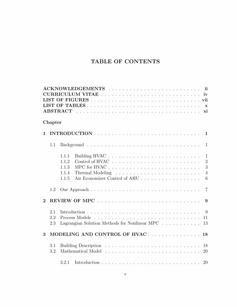
TABLE OF CONTENTS

ACKNOWLEDGEMENTS . . . . . . . . . . . . . . . . . . . . . . . . . . iiCURRICULUM VITAE . . . . . . . . . . . . . . . . . . . . . . . . . . . . ivLIST OF FIGURES . . . . . . . . . . . . . . . . . . . . . . . . . . . . . . . viiLIST OF TABLES . . . . . . . . . . . . . . . . . . . . . . . . . . . . . . . . xABSTRACT . . . . . . . . . . . . . . . . . . . . . . . . . . . . . . . . . . . xi

Chapter

1 INTRODUCTION . . . . . . . . . . . . . . . . . . . . . . . . . . . . . . 1

1.1 Background . . . . . . . . . . . . . . . . . . . . . . . . . . . . . . . . 1

1.1.1 Building HVAC . . . . . . . . . . . . . . . . . . . . . . . . . . 11.1.2 Control of HVAC . . . . . . . . . . . . . . . . . . . . . . . . . 21.1.3 MPC for HVAC . . . . . . . . . . . . . . . . . . . . . . . . . . 31.1.4 Thermal Modeling . . . . . . . . . . . . . . . . . . . . . . . . 41.1.5 Air Economizer Control of AHU . . . . . . . . . . . . . . . . . 6

1.2 Our Approach . . . . . . . . . . . . . . . . . . . . . . . . . . . . . . . 7

2 REVIEW OF MPC . . . . . . . . . . . . . . . . . . . . . . . . . . . . . 9

2.1 Introduction . . . . . . . . . . . . . . . . . . . . . . . . . . . . . . . . 92.2 Process Models . . . . . . . . . . . . . . . . . . . . . . . . . . . . . . 112.3 Lagrangian Solution Methods for Nonlinear MPC . . . . . . . . . . . 13

3 MODELING AND CONTROL OF HVAC . . . . . . . . . . . . . . . 18

3.1 Building Description . . . . . . . . . . . . . . . . . . . . . . . . . . . 183.2 Mathematical Model . . . . . . . . . . . . . . . . . . . . . . . . . . . 20

3.2.1 Introduction . . . . . . . . . . . . . . . . . . . . . . . . . . . . 20

v

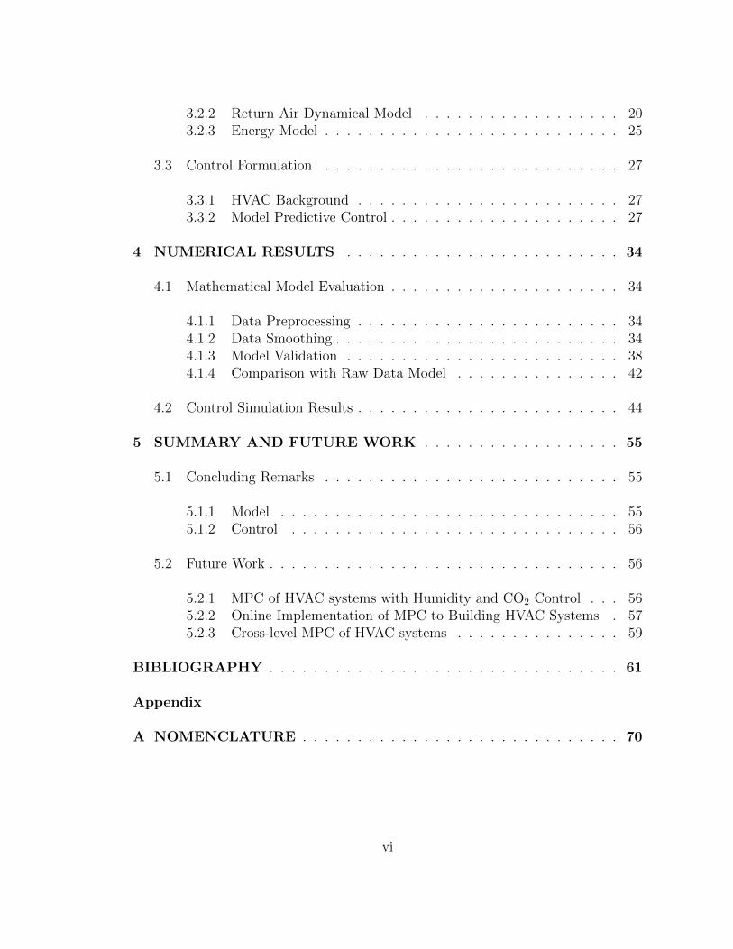
3.2.2 Return Air Dynamical Model . . . . . . . . . . . . . . . . . . 203.2.3 Energy Model . . . . . . . . . . . . . . . . . . . . . . . . . . . 25

3.3 Control Formulation . . . . . . . . . . . . . . . . . . . . . . . . . . . 27

3.3.1 HVAC Background . . . . . . . . . . . . . . . . . . . . . . . . 273.3.2 Model Predictive Control . . . . . . . . . . . . . . . . . . . . . 27

4 NUMERICAL RESULTS . . . . . . . . . . . . . . . . . . . . . . . . . 34

4.1 Mathematical Model Evaluation . . . . . . . . . . . . . . . . . . . . . 34

4.1.1 Data Preprocessing . . . . . . . . . . . . . . . . . . . . . . . . 344.1.2 Data Smoothing . . . . . . . . . . . . . . . . . . . . . . . . . . 344.1.3 Model Validation . . . . . . . . . . . . . . . . . . . . . . . . . 384.1.4 Comparison with Raw Data Model . . . . . . . . . . . . . . . 42

4.2 Control Simulation Results . . . . . . . . . . . . . . . . . . . . . . . . 44

5 SUMMARY AND FUTURE WORK . . . . . . . . . . . . . . . . . . 55

5.1 Concluding Remarks . . . . . . . . . . . . . . . . . . . . . . . . . . . 55

5.1.1 Model . . . . . . . . . . . . . . . . . . . . . . . . . . . . . . . 555.1.2 Control . . . . . . . . . . . . . . . . . . . . . . . . . . . . . . 56

5.2 Future Work . . . . . . . . . . . . . . . . . . . . . . . . . . . . . . . . 56

5.2.1 MPC of HVAC systems with Humidity and CO2 Control . . . 565.2.2 Online Implementation of MPC to Building HVAC Systems . 575.2.3 Cross-level MPC of HVAC systems . . . . . . . . . . . . . . . 59

BIBLIOGRAPHY . . . . . . . . . . . . . . . . . . . . . . . . . . . . . . . . 61

Appendix

A NOMENCLATURE . . . . . . . . . . . . . . . . . . . . . . . . . . . . . 70

vi

LIST OF FIGURES

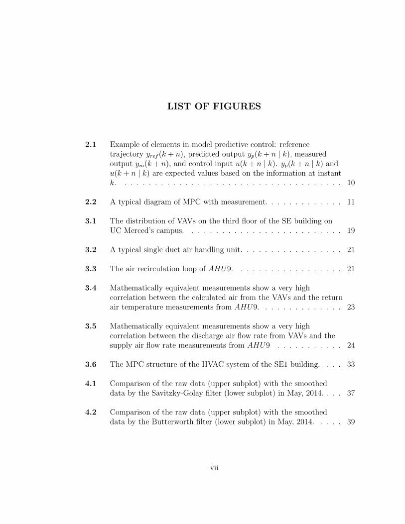
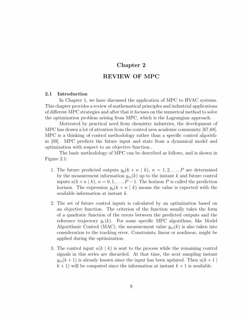
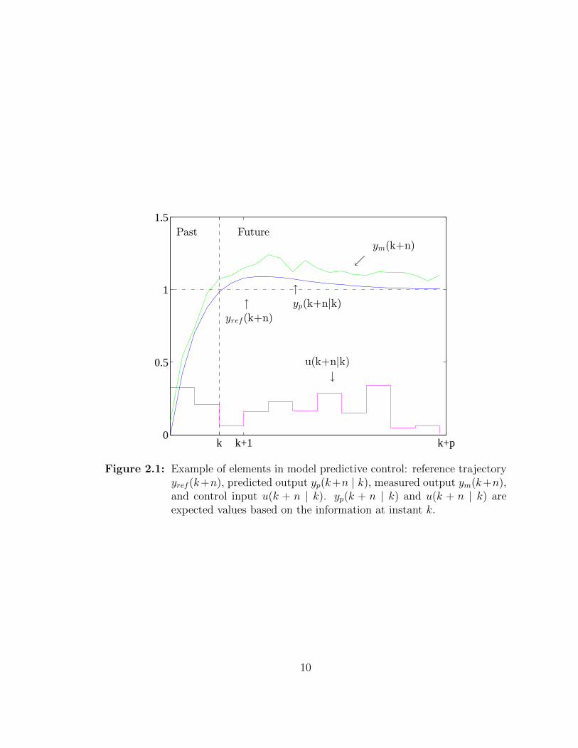
2.1 Example of elements in model predictive control: referencetrajectory yref (k + n), predicted output yp(k + n | k), measuredoutput ym(k + n), and control input u(k + n | k). yp(k + n | k) andu(k + n | k) are expected values based on the information at instantk. . . . . . . . . . . . . . . . . . . . . . . . . . . . . . . . . . . . . 10

2.2 A typical diagram of MPC with measurement. . . . . . . . . . . . . 11

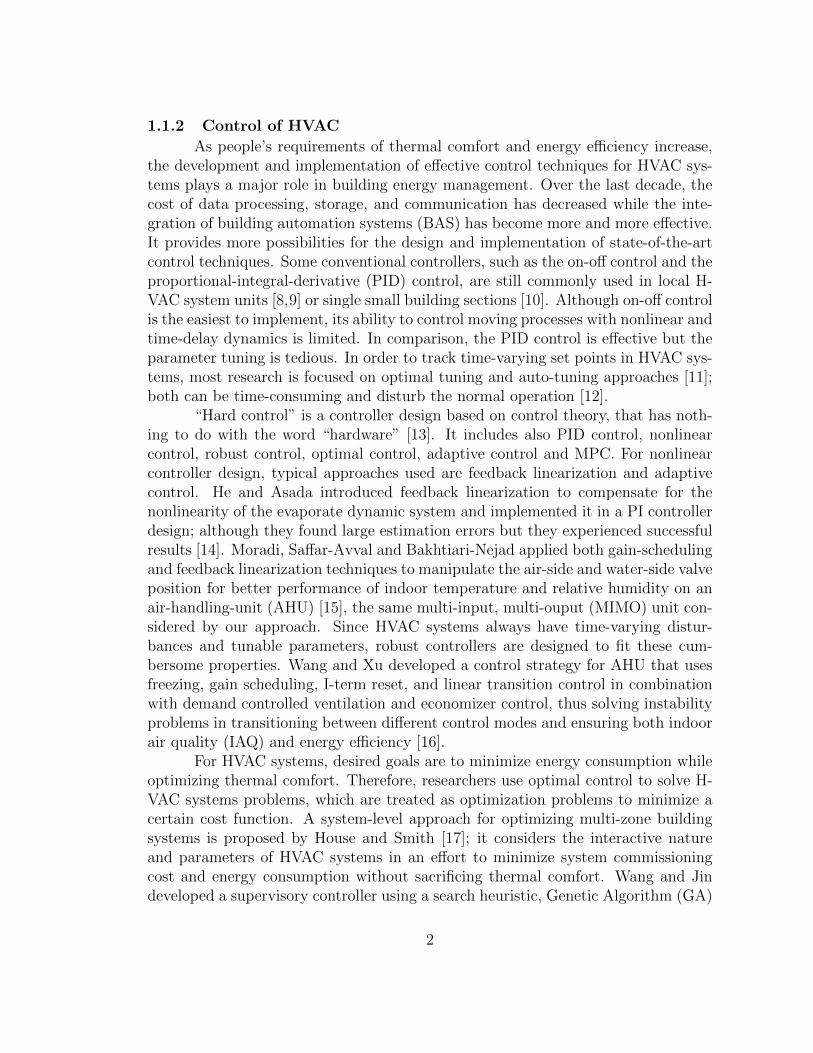
3.1 The distribution of VAVs on the third floor of the SE building onUC Merced’s campus. . . . . . . . . . . . . . . . . . . . . . . . . . 19

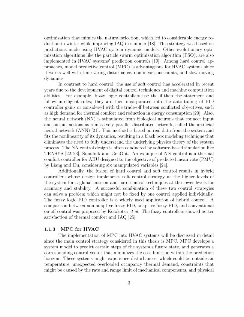
3.2 A typical single duct air handling unit. . . . . . . . . . . . . . . . . 21

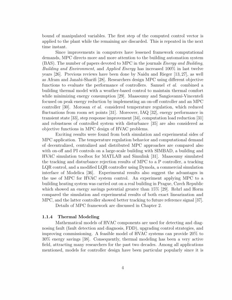
3.3 The air recirculation loop of AHU9. . . . . . . . . . . . . . . . . . 21

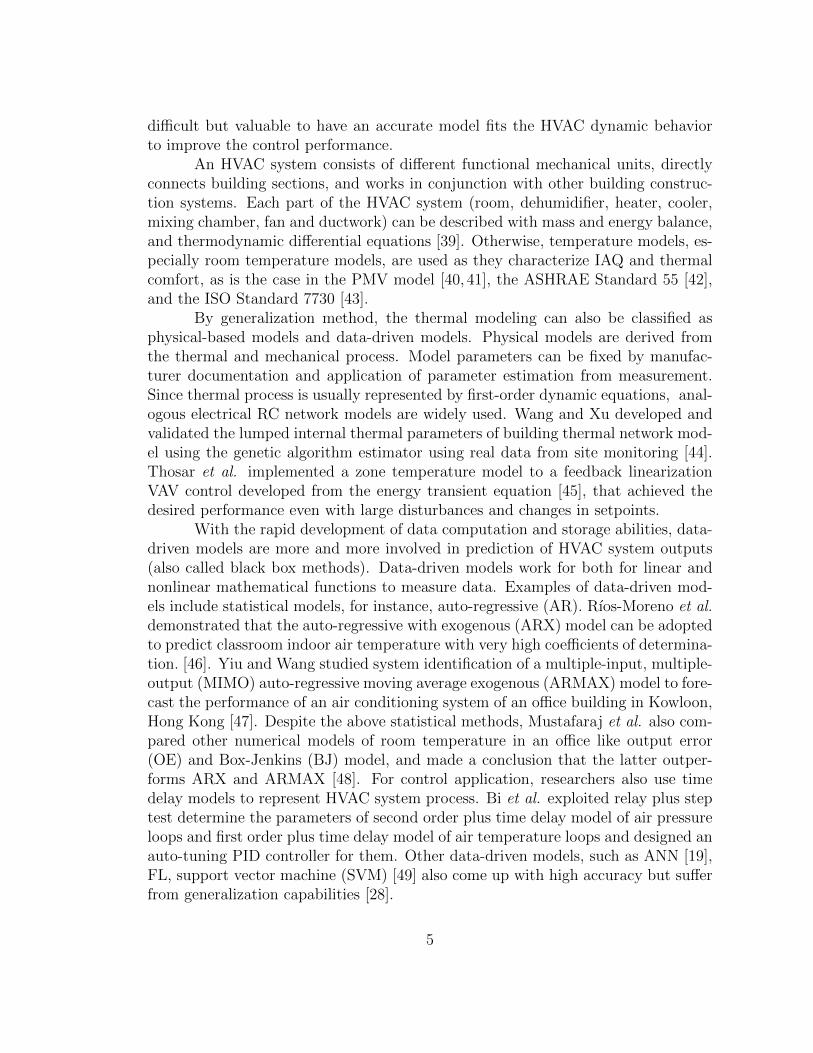
3.4 Mathematically equivalent measurements show a very highcorrelation between the calculated air from the VAVs and the returnair temperature measurements from AHU9. . . . . . . . . . . . . . 23

3.5 Mathematically equivalent measurements show a very highcorrelation between the discharge air flow rate from VAVs and thesupply air flow rate measurements from AHU9 . . . . . . . . . . . 24

3.6 The MPC structure of the HVAC system of the SE1 building. . . . 33

4.1 Comparison of the raw data (upper subplot) with the smootheddata by the Savitzky-Golay filter (lower subplot) in May, 2014. . . . 37

4.2 Comparison of the raw data (upper subplot) with the smootheddata by the Butterworth filter (lower subplot) in May, 2014. . . . . 39

vii

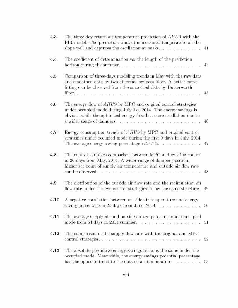
4.3 The three-day return air temperature prediction of AHU9 with theFIR model. The prediction tracks the measured temperature on theslope well and captures the oscillation at peaks. . . . . . . . . . . . 41

4.4 The coefficient of determination vs. the length of the predictionhorizon during the summer. . . . . . . . . . . . . . . . . . . . . . . 43

4.5 Comparison of three-days modeling trends in May with the raw dataand smoothed data by two different low-pass filter. A better curvefitting can be observed from the smoothed data by Butterworthfilter. . . . . . . . . . . . . . . . . . . . . . . . . . . . . . . . . . . . 45

4.6 The energy flow of AHU9 by MPC and original control strategiesunder occupied mode during July 1st, 2014. The energy savings isobvious while the optimized energy flow has more oscillation due toa wider usage of dampers. . . . . . . . . . . . . . . . . . . . . . . . 46

4.7 Energy consumption trends of AHU9 by MPC and original controlstrategies under occupied mode during the first 9 days in July, 2014.The average energy saving percentage is 25.7%. . . . . . . . . . . . 47

4.8 The control variables comparison between MPC and existing controlin 26 days from May, 2014. A wider range of damper position,higher set point of supply air temperature and outside air flow ratecan be observed. . . . . . . . . . . . . . . . . . . . . . . . . . . . . 48

4.9 The distribution of the outside air flow rate and the recirculation airflow rate under the two control strategies follow the same structure. 49

4.10 A negative correlation between outside air temperature and energysaving percentage in 20 days from June, 2014. . . . . . . . . . . . . 50

4.11 The average supply air and outside air temperatures under occupiedmode from 64 days in 2014 summer. . . . . . . . . . . . . . . . . . 51

4.12 The comparison of the supply flow rate with the original and MPCcontrol strategies. . . . . . . . . . . . . . . . . . . . . . . . . . . . . 52

4.13 The absolute predictive energy savings remains the same under theoccupied mode. Meanwhile, the energy savings potential percentagehas the opposite trend to the outside air temperature. . . . . . . . 53

viii

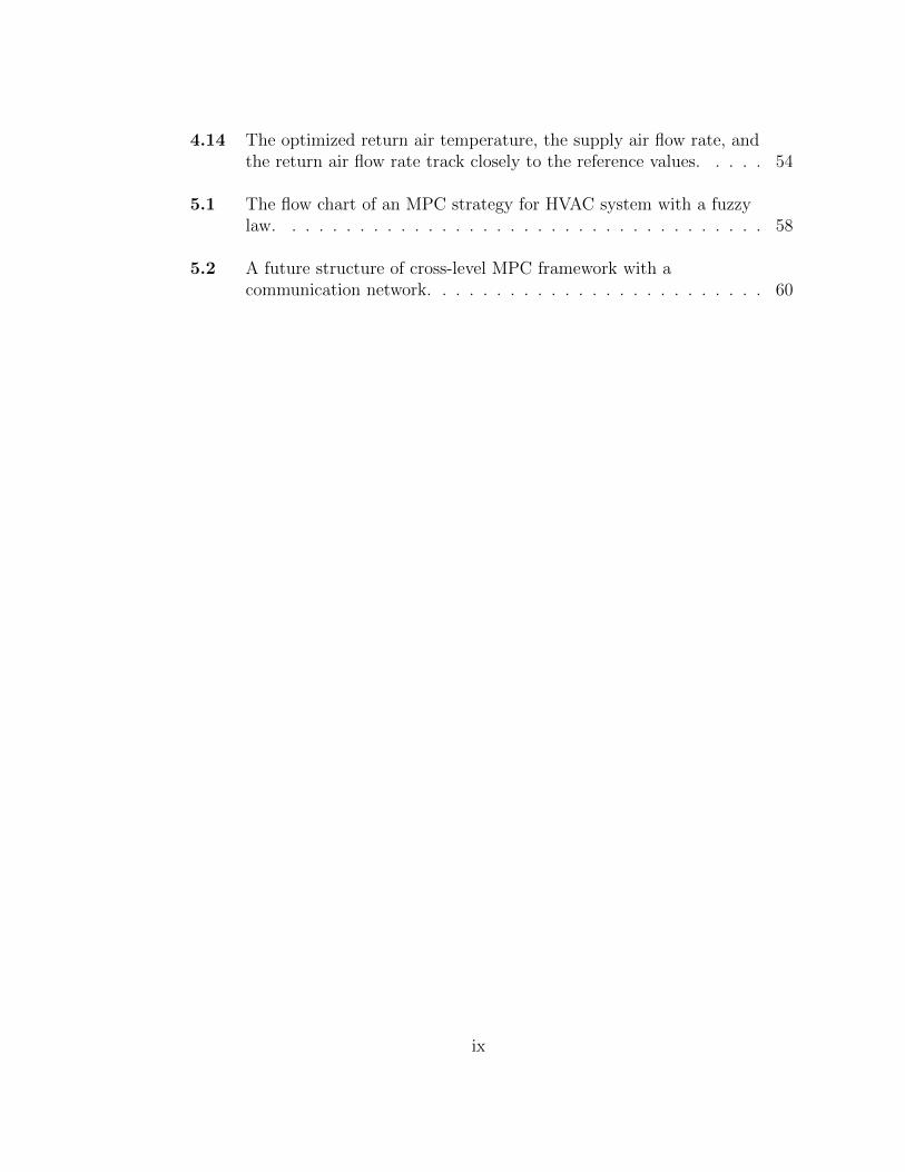
4.14 The optimized return air temperature, the supply air flow rate, andthe return air flow rate track closely to the reference values. . . . . 54

5.1 The flow chart of an MPC strategy for HVAC system with a fuzzylaw. . . . . . . . . . . . . . . . . . . . . . . . . . . . . . . . . . . . 58

5.2 A future structure of cross-level MPC framework with acommunication network. . . . . . . . . . . . . . . . . . . . . . . . . 60

ix

LIST OF TABLES

3.1 The geometries of the rooms or spaces controlled by VAVs of AHU 9. 19

4.1 The errors of the return air temperature prediction of multiplemonths. . . . . . . . . . . . . . . . . . . . . . . . . . . . . . . . . . 41

4.2 The return air temperature prediction error over different predictionhorizons. . . . . . . . . . . . . . . . . . . . . . . . . . . . . . . . . . 43

4.3 The return air flow rate modeling error with respect to raw data andsmoothed data. . . . . . . . . . . . . . . . . . . . . . . . . . . . . . 44

4.4 The tracking MAE of MPC control states to the reference values. . 54

x

ABSTRACT

Heating, ventilation and air conditioning (HVAC) is a mechanical systemthat provides thermal comfort and accepted indoor air quality often instrumentedfor large-scale buildings. The HVAC system takes a dominant portion of overallbuilding energy consumption and accounts for 50% of the energy used in the U.S.commercial and residential buildings in 2012. The performance and energy savingof building HVAC systems can be significantly improved by the implementation ofbetter and smarter control strategies. Therefore, it is of great benefits to developingautomatic, intelligent, optimal and consistent model and control tools to ensure thenormal operations of HVAC systems and increase the building energy efficiency.

Motivated by these goals, this thesis presents a parametric modeling approachand a system-level control design for HVAC systems. For the modeling, we establishdynamical models for return air for the air-handling-unit (AHU) of HVAC systems.The models include temperature and air flow rate models. These models followthe structure of the finite impulse response (FIR) model, and explicitly includethe control variables from the AHU, the dynamical states, and the disturbances.Therefore, it is easy to apply this model to control design. Also, the model isflexible with prediction horizon and control horizon with a stability of the accuracy.In data processing, a convolution-based low-pass digital filter, Savitzky-Golay filter,and the Butterworth low-pass filter are used for data smoothing. As a result, thereturn air flow rate model becomes more feasible with the smoothed data.

Secondly, this thesis study develops a model predictive control (MPC) algo-rithm with the application of the dynamical models for AHU optimization problems.This control strategy optimizes the energy consumption of the AHU, and tracks theset points the room temperatures, supply air flow and return air flow rate of thebuilding. The strategy provides physical-based inherent connection between compo-nents in AHU by applying damper positions, supply air temperature and outside airflow rate as manipulated variables. The control inputs are explicitly implementedinto both the models and objective functions and the optimization structure is com-putationally efficient. The optimal results show an energy saving average percentageover 27.8% and track the supply air flow rate and set point of room temperaturesin the building effectively. The thermal load, supply air flow rate set points are cal-culated from thirty-two VAVs, that ensures the internal cooling demand, the staticpressure, and the ventilation level of the building.

xi

In this thesis, all the data processing and modeling, model validation andimplementation of the control algorithm are based on extensive data measurementscollected from an office building on the campus of the University of California, atMerced. The control strategy is implemented into the online building automationsystem (BAS) of the building and can be easily incorporated with other BAS as wellbecause of the explicit formulation.

xii

Chapter 1

INTRODUCTION

1.1 Background

1.1.1 Building HVAC

Heating, ventilation, and air conditioning (HVAC) is a technology of indoorenvironmental comfort. HVAC is implemented for both residential and commercialbuildings to maintain acceptable thermal comfort within reasonable installation,operation and maintenance costs.

Ever since the invention of its components during the industrial revolution,HVAC has gradually evolved into a highly interdisciplinary and complex system.Numerous new components, advanced sensing technologies, advanced control algo-rithms, and artificial intelligence have been introduced into HVAC to meet oper-ational objectives in different types of buildings worldwide. Consequently, HVACsystems have been extensively deployed in both developed and developing countries.In the United States alone, HVAC systems condition a total area of nearly 3.1 billionsquare feet in buildings [1].

Due to increasing global population growth and civilization, more and morelarge-scale buildings are being built all over the world. Buildings have become oneof the fastest growing energy consuming facilities on the earth. According to theU.S. Department of Energy’s 2011 Building Energy Databook, buildings use 74%of the nation’s electricity, and 40.33% of the nation’s total energy consumptionwhich is valued at $431.1 billion [2–4]. HVAC systems make up almost 50% of theenergy used in U.S. commercial and residential buildings [5]. Both organizations andgovernments put their efforts to reduce the energy consumption of HVAC systems.For example, the primary professional organization for regulation and standard ofHVAC industry in the U.S., the American Society of Heating, Refrigerating andAir-Conditioning Engineers (ASHRAE), has published ASHRAE Standard 90.1 [6]to provide minimum requirements for energy efficient design for buildings includingthe HVAC part. And the application of the California Energy Commission’s energyefficiency standards code title 24 has saved Californians more than $74 billion inreduced electricity since 1977 [7]. As such, bettering the efficiency of HVAC systemscan significantly reduce the amount of electricity and energy buildings consume.The performance and energy saving of building HVAC systems can be significantlyimproved by the implementation of better and smarter control strategies.

1

1.1.2 Control of HVAC

As people’s requirements of thermal comfort and energy efficiency increase,the development and implementation of effective control techniques for HVAC sys-tems plays a major role in building energy management. Over the last decade, thecost of data processing, storage, and communication has decreased while the inte-gration of building automation systems (BAS) has become more and more effective.It provides more possibilities for the design and implementation of state-of-the-artcontrol techniques. Some conventional controllers, such as the on-off control and theproportional-integral-derivative (PID) control, are still commonly used in local H-VAC system units [8,9] or single small building sections [10]. Although on-off controlis the easiest to implement, its ability to control moving processes with nonlinear andtime-delay dynamics is limited. In comparison, the PID control is effective but theparameter tuning is tedious. In order to track time-varying set points in HVAC sys-tems, most research is focused on optimal tuning and auto-tuning approaches [11];both can be time-consuming and disturb the normal operation [12].

“Hard control” is a controller design based on control theory, that has noth-ing to do with the word “hardware” [13]. It includes also PID control, nonlinearcontrol, robust control, optimal control, adaptive control and MPC. For nonlinearcontroller design, typical approaches used are feedback linearization and adaptivecontrol. He and Asada introduced feedback linearization to compensate for thenonlinearity of the evaporate dynamic system and implemented it in a PI controllerdesign; although they found large estimation errors but they experienced successfulresults [14]. Moradi, Saffar-Avval and Bakhtiari-Nejad applied both gain-schedulingand feedback linearization techniques to manipulate the air-side and water-side valveposition for better performance of indoor temperature and relative humidity on anair-handling-unit (AHU) [15], the same multi-input, multi-ouput (MIMO) unit con-sidered by our approach. Since HVAC systems always have time-varying distur-bances and tunable parameters, robust controllers are designed to fit these cum-bersome properties. Wang and Xu developed a control strategy for AHU that usesfreezing, gain scheduling, I-term reset, and linear transition control in combinationwith demand controlled ventilation and economizer control, thus solving instabilityproblems in transitioning between different control modes and ensuring both indoorair quality (IAQ) and energy efficiency [16].

For HVAC systems, desired goals are to minimize energy consumption whileoptimizing thermal comfort. Therefore, researchers use optimal control to solve H-VAC systems problems, which are treated as optimization problems to minimize acertain cost function. A system-level approach for optimizing multi-zone buildingsystems is proposed by House and Smith [17]; it considers the interactive natureand parameters of HVAC systems in an effort to minimize system commissioningcost and energy consumption without sacrificing thermal comfort. Wang and Jindeveloped a supervisory controller using a search heuristic, Genetic Algorithm (GA)

2

optimization that mimics the natural selection, which led to considerable energy re-duction in winter while improving IAQ in summer [18]. This strategy was based onpredictions made using HVAC system dynamic models. Other evolutionary opti-mization algorithms like the particle swarm optimization algorithm (PSO), are alsoimplemented in HVAC systems’ prediction controls [19]. Among hard control ap-proaches, model predictive control (MPC) is advantageous for HVAC systems sinceit works well with time-varing disturbance, nonlinear constraints, and slow-movingdynamics.

In contrast to hard control, the use of soft control has accelerated in recentyears due to the development of digital control techniques and machine computationabilities. For example, fuzzy logic controllers use the if-then-else statement andfollow intelligent rules; they are then incorporated into the auto-tuning of PIDcontroller gains or considered with the trade-off between conflicted objectives, suchas high demand for thermal comfort and reduction in energy consumption [20]. Also,the neural network (NN) is stimulated from biological neurons that connect inputand output actions as a massively parallel distributed network, called the artificialneural network (ANN) [21]. This method is based on real data from the system andfits the nonlinearity of its dynamics, resulting in a black box modeling technique thateliminates the need to fully understand the underlying physics theory of the systemprocess. The NN control design is often conducted by software-based simulation likeTRNSYS [22, 23], Simulink and GenOpt. An example of NN control is a thermalcomfort controller for AHU designed to the objective of predicted mean vote (PMV)by Liang and Du, considering six manipulated variables [24].

Additionally, the fusion of hard control and soft control results in hybridcontrollers whose design implements soft control strategy at the higher levels ofthe system for a global mission and hard control techniques at the lower levels foraccuracy and stability. A successful combination of these two control strategiescan solve a problem which might not be fixed by one control applied individually.The fuzzy logic PID controller is a widely used application of hybrid control. Acomparison between non-adaptive fuzzy PID, adaptive fuzzy PID, and conventionalon-off control was proposed by Kolokotsa et al. The fuzzy controllers showed bettersatisfaction of thermal comfort and IAQ [25].

1.1.3 MPC for HVAC

The implementation of MPC into HVAC systems will be discussed in detailsince the main control strategy considered in this thesis is MPC. MPC develops asystem model to predict certain steps of the system’s future state, and generates acorresponding control vector that minimizes the cost function within the predictionhorizon. These systems might experience disturbances, which could be outside airtemperature, unexpected overloaded occupancy thermal demand, constraints thatmight be caused by the rate and range limit of mechanical components, and physical

3

bound of manipulated variables. The first step of the computed control vector isapplied to the plant while the remaining are discarded. This is repeated in the nexttime instant.

Since improvements in computers have lessened framework computationaldemands, MPC directs more and more attention to the building automation system(BAS). The number of papers devoted to MPC in the journals Energy and Building,Building and Environment, and Applied Energy has increased 100% in last twelveyears [26]. Previous reviews have been done by Naidu and Rieger [13, 27], as wellas Afram and Janabi-Sharifi [28]. Researchers design MPC using different objectivefunctions to evaluate the performance of controllers. Samuel et al. combined abuilding thermal model with a weather-based control to maintain thermal comfortwhile minimizing energy consumption [29]. Maasoumy and Sangiovanni-Vincentelifocused on peak energy reduction by implementing an on-off controller and an MPCcontroller [30]. Morosan et al. considered temperature regulation, which reducedfluctuations from room set points [31]. Moreover, IAQ [32], energy performance intransient state [33], step response improvement [34], computation load reduction [31]and robustness of controlled system with disturbance [35] are also considered asobjective functions in MPC design of HVAC problems.

Exciting results were found from both simulation and experimental sides ofMPC application. The temperature regulation behavior and computational demandof decentralized, centralized and distributed MPC approaches are compared alsowith on-off and PI controls on a large-scale building with SIMBAD, a building andHVAC simulation toolbox for MATLAB and Simulink [31]. Maasoumy simulatedthe tracking and disturbance rejection results of MPC to a P controller, a trackingLQR control, and a modified LQR controller using Dymola, a commercial simulationinterface of Modelica [36]. Experimental results also suggest the advantages inthe use of MPC for HVAC system control. An experiment applying MPC to abuilding heating system was carried out on a real building in Prague, Czech Republicwhich showed an energy savings potential greater than 15% [29]. Rehrl and Hormcompared the simulation and experimental results of both exact linearization andMPC, and the latter controller showed better tracking to future reference signal [37].

Details of MPC framework are discussed in Chapter 2.

1.1.4 Thermal Modeling

Mathematical models of HVAC components are used for detecting and diag-nosing fault (fault detection and diagnosis, FDD), upgrading control strategies, andimproving commissioning. A feasible model of HVAC systems can provide 20% to30% energy savings [38]. Consequently, thermal modeling has been a very activefield, attracting many researchers for the past two decades. Among all applicationsmentioned, models for controller design have been particular popularly since it is

4

difficult but valuable to have an accurate model fits the HVAC dynamic behaviorto improve the control performance.

An HVAC system consists of different functional mechanical units, directlyconnects building sections, and works in conjunction with other building construc-tion systems. Each part of the HVAC system (room, dehumidifier, heater, cooler,mixing chamber, fan and ductwork) can be described with mass and energy balance,and thermodynamic differential equations [39]. Otherwise, temperature models, es-pecially room temperature models, are used as they characterize IAQ and thermalcomfort, as is the case in the PMV model [40, 41], the ASHRAE Standard 55 [42],and the ISO Standard 7730 [43].

By generalization method, the thermal modeling can also be classified asphysical-based models and data-driven models. Physical models are derived fromthe thermal and mechanical process. Model parameters can be fixed by manufac-turer documentation and application of parameter estimation from measurement.Since thermal process is usually represented by first-order dynamic equations, anal-ogous electrical RC network models are widely used. Wang and Xu developed andvalidated the lumped internal thermal parameters of building thermal network mod-el using the genetic algorithm estimator using real data from site monitoring [44].Thosar et al. implemented a zone temperature model to a feedback linearizationVAV control developed from the energy transient equation [45], that achieved thedesired performance even with large disturbances and changes in setpoints.

With the rapid development of data computation and storage abilities, data-driven models are more and more involved in prediction of HVAC system outputs(also called black box methods). Data-driven models work for both for linear andnonlinear mathematical functions to measure data. Examples of data-driven mod-els include statistical models, for instance, auto-regressive (AR). Rıos-Moreno et al.demonstrated that the auto-regressive with exogenous (ARX) model can be adoptedto predict classroom indoor air temperature with very high coefficients of determina-tion. [46]. Yiu and Wang studied system identification of a multiple-input, multiple-output (MIMO) auto-regressive moving average exogenous (ARMAX) model to fore-cast the performance of an air conditioning system of an office building in Kowloon,Hong Kong [47]. Despite the above statistical methods, Mustafaraj et al. also com-pared other numerical models of room temperature in an office like output error(OE) and Box-Jenkins (BJ) model, and made a conclusion that the latter outper-forms ARX and ARMAX [48]. For control application, researchers also use timedelay models to represent HVAC system process. Bi et al. exploited relay plus steptest determine the parameters of second order plus time delay model of air pressureloops and first order plus time delay model of air temperature loops and designed anauto-tuning PID controller for them. Other data-driven models, such as ANN [19],FL, support vector machine (SVM) [49] also come up with high accuracy but sufferfrom generalization capabilities [28].

5

It is natural to consider combining the strength of the physical-based modeland the data-driven numerical approach. Wu and Sun proposed different multi-stage regression, physical-based linear parametric (mpbARMAX) models of roomtemperature and PMV index to take the advantage of both analytical and numericalmodeling approaches. The multi-stage regression structure also reveals the relation-ship between the building thermal performance and the building parameters [50–53].

For MPC, the choice of thermal modeling also plays a key role in the wholecontrol process. A detailed building model from building structure, mechanicalcomponents and material, might work effectively for subsystems by computer-aidedmodeling tools, i.e. TRNSYS [22] and EnergyPlus [54], and simulates and tracksthe building system behavior. However, the implicity and complexity of the modelsreduce its possibility to implement with MPC strategy [26].

1.1.5 Air Economizer Control of AHU

The control problems in HVAC systems can also be classified from the struc-ture side rather than methodology side. Over the last decade, there have beenconsiderable research and development on model-based and optimal control algo-rithms for both HVAC equipments at the component level and system level. Acomplex HVAC system of a commercial building consists of cooling towers, chillers,AHUs, and zones with VAV units. Research on optimal control for cooling towersand chillers can be found in the work by Chow et al. [55] and Jin et al. [56] respec-tively. Within VAV, MPC approach by Huang [35] and GA optimization by Wangand Jin [18] are implemented.

Unlike other units, the AHU is multi-functional and nexus between centralplant and building level of HVAC systems. An AHU is used to regulate, distribute,and recirculate air of an HVAC system. It includes different types of components,such as air dampers, fans, heating or cooling coils, humidifier, filters and mixingchamber. If an AHU uses 100% outside air and doesn’t recirculate air, it is calleda makeup air unit (MAU). Also, an AHU designed for outdoor use, usually onroofs, is known as a packaged unit (PU) or rooftop unit (RTU). Building EnergySystems Group of the Pacific Northwest National Laboratory (PNNL) estimated theenergy and cost savings for RTUs from different control strategies individually andin combination using EnergyPlus for four building types in 16 locations coveringall 15 climate zones in the U.S. [57]. Four control options, economizer control, fanspeed control, cooling capacity control, and demand-controlled ventilation (DCV)were compared. The result showed that simply adding multi-speed fan control andDCV individually contribute the most to energy and cost saving for PUs.

As for typical AHUs, similar as control types mentioned from PNNL’s work,fan control, cooling coil control, and air economizer control are applied. Bai etal. built a second-order plus dead-time plant representing the dynamics from the

6

supply fan variable speed drive to the supply air pressure, then implemented an auto-tuning PID controller on it [11]. The results demonstrated the superior performanceof the auto-tuner over the manually tuned PID controller. With regard to coolingcoil control, Wang et al. derived a simplified model from energy balance and heattransfer principles followed by parameter identification by either linear and nonlinearleast square method [58]. The model is easy to apply to real-time cooling coilcontrol since it contains the set points from the air side and the water side, and canserve as constraints in energy consumption optimization. Fong et al. implementan evolutionary programming technique in cooling coil control by optimizing boththe set points of chilled water and supply air temperatures on a monthly basis, andachieved 7% saving potential compared to the one with the existing settings [59].

Last but not least, the air economizer takes in outside air to reduce mechan-ical cooling energy consumption and can be controlled easily by adjusting outsideair damper, exhaust air damper, and recirculation air damper positions. The per-formance of an air economizer directly impacts on the electricity consumption offans and cooling coil. Therefore, it has a great potential in energy and cost sav-ing, and draws attention from researchers over the last two decades. Engineers inJohnson Controls presented a damper control system considering damper geometry,dynamic losses and pressure drop to prevent outside air entering the AHU throughthe exhaust duct [60]. Wang and Liu considered humidity control during an aireconomizer cycle to achieve IAQ requirements with a less energy price [61]. Yuanand Perez introduced MPC to the air economizer control with supply air temper-ature and outside air flow rate as control variables, that showed a cost effectiveperformance compared to tradition PI controller [62]. Nassif and Moujaes devel-oped a split-signal damper control theory [63]. The new operation strategy showedan annual energy saving and better fan performance compared to the conventionaltwo-couple and three-coupled damper tuning approaches [64]. Seem and House sim-ulated the model-based and the optimization-based control strategies to minimizecooling load by adjusting outside air fraction [65]. Wang and Song talked aboutderivative-based supply air flow rate and supply air temperature optimal controlduring an air economizer cycle in the case of MAU [66].

1.2 Our Approach

The pursuit of building energy efficiency and thermal comfort provides mo-tivation for us to achieve a system-level modeling and control of HVAC system.

For the modeling, a parametric ARMAX model is presented for return airtemperature and return air flow rate in an AHU. The resulting models take advan-tages of data-driven technique and are easy for control design implementation. Asa result, the models fit the measurements pretty well and serve as the plant modelin MPC algorithm with a flexibility of prediction horizon length.

7

For the control, a system-level MPC is designed for an HVAC system. Bymodeling the dynamics inside AHU and applying objectives and constraints fromthe lower level HVAC units, this control strategy links different levels of the HVACsystem with a focus on energy consumption. Also, the computation load is low sincethe models and objective functions are explicit and the gradient inside this optimalcontrol follows a fine structure. This control strategy reduces energy consumptionmeanwhile secure the enough cooling load, pressure balance, and thermal comfortof the building.

The rest of this thesis consists of four chapters. Chapter 2 presents theintroduction of MPC, mathematical models commonly used in MPC, and a specialMPC approach with Lagrangian Multiplier. Chapter 3 implements the ARMAXmodel of HVAC dynamics and MPC control with Lagrangian Multiplier to an HVACsystem. Chapter 4 demonstrates the model validation and control simulation resultsbased on data collected from a building on the campus of University of California(UC) at Merced. Finally, Chapter 5 summarize this thesis and take a look at thefuture work.

8

Chapter 2

REVIEW OF MPC

2.1 Introduction

In Chapter 1, we have discussed the application of MPC to HVAC systems.This chapter provides a review of mathematical principles and industrial applicationsof different MPC strategies and after that it focuses on the numerical method to solvethe optimization problem arising from MPC, which is the Lagrangian approach.

Motivated by practical need from chemistry industries, the development ofMPC has drawn a lot of attention from the control area academic community [67,68].MPC is a thinking of control methodology rather than a specific control algorith-m [69]. MPC predicts the future input and state from a dynamical model andoptimization with respect to an objective function..

The basic methodology of MPC can be described as follows, and is shown inFigure 2.1:

1. The future predicted outputs yp(k + n | k), n = 1, 2, . . . , P are determinedby the measurement information ym(k) up to the instant k and future controlinputs u(k+n | k), n = 0, 1, . . . , P − 1. The horizon P is called the predictionhorizon. The expression yp(k + n | k) means the value is expected with theavailable information at instant k.

2. The set of future control inputs is calculated by an optimization based onan objective function. The criterion of the function usually takes the formof a quadratic function of the errors between the predicted outputs and thereference trajectory yr(k). For some specific MPC algorithms, like ModelAlgorithmic Control (MAC), the measurement value ym(k) is also taken intoconsideration to the tracking error. Constraints, linear or nonlinear, might beapplied during the optimization.

3. The control input u(k | k) is sent to the process while the remaining controlsignals in this series are discarded. At that time, the next sampling instantym(k + 1) is already known since the input has been updated. Then u(k + 1 |k + 1) will be computed since the information at instant k + 1 is available.

9

k k+1 k+p0

0.5

1

1.5Past Future

↑

yp(k+n|k)

yref(k+n)

↑

ւ

ym(k+n)

↓

u(k+n|k)

Figure 2.1: Example of elements in model predictive control: reference trajectoryyref (k+n), predicted output yp(k+n | k), measured output ym(k+n),and control input u(k + n | k). yp(k + n | k) and u(k + n | k) areexpected values based on the information at instant k.

10

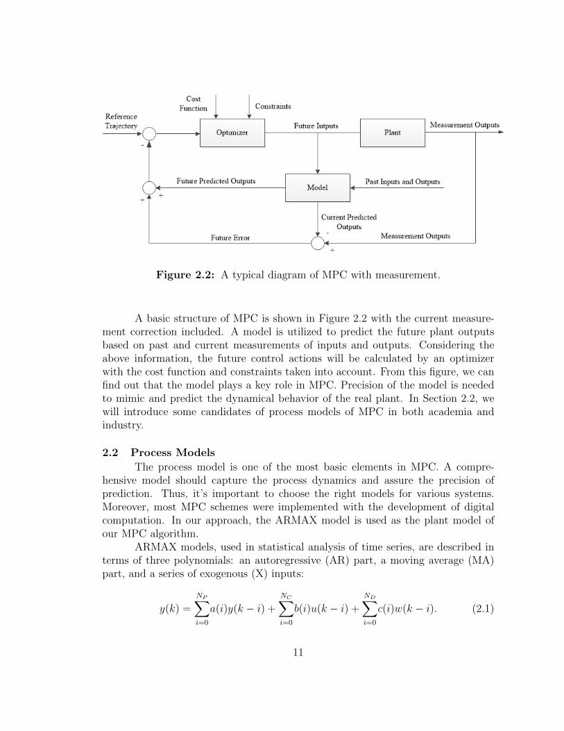
Figure 2.2: A typical diagram of MPC with measurement.

A basic structure of MPC is shown in Figure 2.2 with the current measure-ment correction included. A model is utilized to predict the future plant outputsbased on past and current measurements of inputs and outputs. Considering theabove information, the future control actions will be calculated by an optimizerwith the cost function and constraints taken into account. From this figure, we canfind out that the model plays a key role in MPC. Precision of the model is neededto mimic and predict the dynamical behavior of the real plant. In Section 2.2, wewill introduce some candidates of process models of MPC in both academia andindustry.

2.2 Process Models

The process model is one of the most basic elements in MPC. A compre-hensive model should capture the process dynamics and assure the precision ofprediction. Thus, it’s important to choose the right models for various systems.Moreover, most MPC schemes were implemented with the development of digitalcomputation. In our approach, the ARMAX model is used as the plant model ofour MPC algorithm.

ARMAX models, used in statistical analysis of time series, are described interms of three polynomials: an autoregressive (AR) part, a moving average (MA)part, and a series of exogenous (X) inputs:

y(k) =

NP∑i=0

a(i)y(k − i) +

NC∑i=0

b(i)u(k − i) +

ND∑i=0

c(i)w(k − i). (2.1)

11

where y(k− i) is the output sequence, u(k− i) is the external inputs, and w(k− i) isthe disturbance. This model contains the states order NP , the controls inputs orderNC , and the disturbance inputs order NC , and coefficients a(i), b(i), c(i) respectively.Typically they must be obtained by fitting the model to plant data. Obviously,a(0) = b(0) = c(0) = 0.

If there is no disturbance included, the model can be represented as

y(k) =

NP∑i=0

a(i)y(k − i) +

NC∑i=0

b(i)u(k − i). (2.2)

This model is also called the Infinite Impulse Response (IIR) filter since it has aninternal feedback to continue the impulse infinitely. Compared to Finite ImpulseResponse (FIR) filter, IIR filter meets a given set of specifications with a much lowerfilter order than a corresponding FIR filter. Moreover, the IIR filter contains thehistory of state error, which makes it trackable to the measurement noise, but needsto update online with a steep adaptation.

The IIR filter model is equivalent to different models, such as state spacemodels and transfer functions [70]. Given the concept of state space in linear controltheory, the model can be rewritten as a state space model

x(k) = Ax(k − 1) +Bu(k − 1), (2.3)

y(k) = Cx(k).

Similarly, if the time delay of control input is considered, the transfer functionmodel can be shown as

y(z) =z−mB(z−1)

A(z−1)u(z), (2.4)

where A(z−1) and B(z−1) are polynomials of z-transform variable, m is the time de-lay. If m = 0, this model is equivalent to Equations 2.2 and 2.3. The parameter canbe determined by experimental identification. However, to build this model, someprior knowledge should be considered such as the order of A(z−1) and B(z−1) [69].This model is often used in Generalized Predictive Control (GPC), Unified Predic-tive Control (UPC) and Extended Prediction Self-Adaptive Control (EPSAC).

Moreover, if a(i) = 0, i = 1, . . . , NP and c(i) = 0, i = 1, . . . , ND, the modelcan be described as the impulse response model, also called the finite convolutionmodel. It represents the output by a weighted sequence of previous inputs at differ-ent time intervals. It appears in MAC. The relationship between output and inputis given by

y(k) =k∑i=0

g(i)u(k − i). (2.5)

12

This model is also known as the FIR filter. The response of an FIR filter to animpulse ultimately settles to zero because there is no feedback in the filter. TheFIR filter can be written as the step response model

y(k) =k∑i=0

β(i)∆u(k − i), (2.6)

where the parameter β(i) known as the process step-response function; and ∆u(k−i) = u(k− i)−u(k− i− 1). The step response model is commonly used in DynamicMatrix Control (DMC) and its variants. It’s easy to find its similarity to the impulseresponse model. They are equivalent [67] and connected as

g(i) = β(i)− β(i− 1), (2.7)

β(i) =i∑

j=1

g(j). (2.8)

To conclude, ARMAX model consists of the previous states, the control in-puts and also disturbance. The properties ensure its ability to be adopted to MPCalgorithm. Its equivalence to other models also provides the possibility to rebuildthe model in different MPC strategy application and for different controller designobjectives.

2.3 Lagrangian Solution Methods for Nonlinear MPC

The concept of Lagrangian Multiplier Methods stems from mathematicaloptimization for finding the local minima and maxima of a function subject tosome equality constraints. The minimization of the optimization problem can beexpressed as:

minx∈D

f(x, y), (2.9)

g(x, y) = c, (2.10)

where f(x, y) is the function needs optimization, subject to the constraint g(x, y) =c.

If f(x, y) and g(x, y) are continuous and first partial derivable, we can in-troduce a new variable λ as the Lagrangian Multiplier. The new objective is theLagrange function defined by

L(x, y, λ) = f(x, y) + λ(g(x, y)− c), (2.11)

The gradients of Lagrange function respective to x, y, λ can be derived as:

13

∂L∂x

= ∂f∂x

+ λ ∂g∂x,

∂L∂y

= ∂f∂y

+ λ∂g∂y,

∂L∂λ

= g(x, y).

(2.12)

The extremum is found by solving the 3 equations in 3 unknowns x, y, and theLagrangian Multiplier λ. From Equation 2.12 it is easy to find that the gradient vec-tors of f(x, y) and g(x, y) are parallel, although their magnitudes are unequal. Notethat the case λ = 0 is also a solution regardless of g(x, y). If an extremum exists,the method of Lagrangian Multipliers yields a necessary and sufficient condition foroptimality in this constrained problem [71]. This method is widely used in optimiza-tion problem equality constraints, but if Lagrangian Multipliers are nonnegative italso works for inequality constraints, which are also called as Karush-Kuhn-Tuckerconditions (KKT) [72].

In control theory, the Lagrange Multiplier Method is often applied to formoptimal controllers due to its flexibility to solve both lower and higher dimensionconstrained problems [73, 74]. A typical MPC scheme tries to solve a constrainedoptimization problem at discrete time steps whose decision variables are given asa control input sequence. The objective function is often in the formulation of lin-ear quadratic regulation (LQR), which is easy to implement in Lagrange functions.Thus, an interactive way to compute the optimal manipulated variables is to usethe Lagrangian Multipliers framework. A receding horizon, open-loop optimal MPCcontrol law using Lagrangian Multipliers was introduced by Muske et al. [75]. Theoptimization problem is a nonlinear model with an equality constraint and an in-equality constraint. Tøndel et al. converted a constrained linear MPC problem to amulti-parameter quadratic programming (QP) solver and found explicit MPC solu-tion by applying KKT conditions [76]. Hovd utilized the calculation of 1-norm andinfinite-norm of Lagrangian Multipliers of QP problems to design penalty functionsfor soft constraints in MPC [77]. Richter et al. discussed the certification of a fastgradient method obtained from the Lagrangian Multipliers Method and applied thecertification procedure to a constrained MPC problem under KKT conditions [78].Nedelcu and Necoara developed an approximate dual gradients method to updateLagrangian Multipliers and improved the number of iterations in a quadratic M-PC problem [79]. All of these studies demonstrate that the Lagrangian MultiplierMethod can be a good fit to solve MPC problems, especially for linear models, andsatisfies both equality and inequality constraints.

The formulation of MPC with Lagrange Multipliers can be expressed as fol-lows. In discrete time, a deterministic process control is

x(k + 1) = f(x(k), u(k)), (2.13)

y(k) = g(x(k)).

14

These states x(k) controls u(k) and outputs y(k) are vectors.For a conventional MPC formulation, the objective can be written as

J =N∑j=0

(Φ(y(k + j | k)) +Qj |yr(k + j)− y(k + j | k)|2) (2.14)

+N−1∑j=0

Rj |∆u(k + j | k)|2 .

This objective function contains a nonlinear objective term, the quadraticfunction of the tracking error to reference trajectory, the penalty of the controleffort, where Qj, Rj > 0 are the weights of each term. It should be noted that theobjective function is calculated based on the prediction horizon and follows the formof summation. After introducing Lagrange Multiplier, the objective function can beexpressed as

J∗ = J +N∑j=1

λj(x(k + j | k)− f(x(k + j − 1 | k), u(k + j − 1 | k))). (2.15)

Compared to the original equation 2.14, the Lagrangian term is added, whereλj is the Lagrange Multiplier.

Therefore, the predictive controller solves at each time step the followingoptimization problem:

minx,y,u

J∗(x,y,u, λ) (2.16)

s.t.x(k + j | k)− f(x(k + j − 1 | k), u(k + j − 1 | k)), j = 1, . . . , N, (2.17a)

y(k + j | k) = g(x(k + j | k)), j = 0, . . . , N − 1, (2.17b)

u(k + j | k) ∈ U, k = 0, . . . , N − 1, (2.17c)

x(k + j | k) ∈ X, j = 1, . . . , N, (2.17d)

where U and X imply the bounds and constraints of control inputs and states. Ifthe objective function is explicit to partial differentiation, we can find the gradientof J respect to all the variables:

15

∇J∗ =

∂J∗

∂x(k+N |k)∂J∗

∂x(k+N−1|k)...

∂J∗

∂x(k+1|k)∂J∗

∂u(k+N−1|k)...

∂J∗

∂u(k|k)∂J∗

∂λN...

∂J∗

∂λ1

= 0, (2.18)

X = [x(k +N | k), x(k +N − 1 | k)...x(k + 1 | k),

u(k +N − 1 | k), . . . u(k | k), λN . . . λ1]T . (2.19)

After solving 2.19 from the gradient 2.18, the optimal combination of futurestates, control inputs and Lagrange Multipliers can be found. The computationalload is decided by the length of prediction horizon. The highlight of this method isintroducing the dynamics of the system as a constraint inside the objective function,as the formulation of Lagrange Multiplier. Then the objective function turns to aLagrange function.

Moreover, the structure of ∇J is also computational-friendly. For example,if Φ(y) = 0, y(k) = x(k), we rewrite ∇J∗ = 0 as AX = b,

2QN 0 IN0 R −BT

IN B 0

x(k +N | k)x(k +N − 1 | k)

...x(k + 1 | k)

u(k +N − 1 | k)...

u(k | k)λN...λ1

= b, (2.20)

16

where the penalty matrix

R =

RN−1 −RN−1

RN−2

. . .

R0 R0

, (2.21)

and the N − 1 by N partial derivative matrix B with respect to control variables

B =

∂f(x(k+N |k),u(k+N−1|k))

∂u(k+N−1|k)

. . .∂ 6f(x(k+1|k),u(k|k))

∂u(k|k)

. (2.22)

After solving the linear system 2.20, the future control input array U =[u(k | k), . . . , u(k +N − 1 | k)]T can be calculated.

For controls for HVAC systems, the Lagrange Multiplier is often used withphysical-based and analytical models. Knabe and Felsmann designed an optimaloperation schedule of HVAC systems based on Lagrange Multiplier method, andexpressed the difficulties of its application in the technical field [80]. Marletta com-pared Lagrange Multipliers Method with the Monte Carlo method and Szargut-Tsatsaronis method, and discussed the possibility to use Lagrange Multipliers assensitivity coefficients for HVAC systems’ performance [81]. Chang chose the co-efficient of performance (COP) of a chiller as the objective function, and adoptedLagrange Multiplier with the balance equation of the chiller’s cooling load [82]; theexperiment results on two building in Taipei showed a lower energy cost compared tothe conventional control. As for the utilization of Lagrange Multiplier in the MPCstrategy for HVAC systems, Kelman and Borrelli designed an MPC controller basedon a dynamical model of AHUs with a strong assumption of thermal load in thebuilding zone and outside air temperature [83]. In our approach, the Lagrange Mul-tiplier is combined with the data-driven dynamical model in the objective function,which will be discussed in Chapter 3.

17

Chapter 3

MODELING AND CONTROL OF HVAC

3.1 Building Description

Extensive past and current measurements of the HVAC system in the Scienceand Engineering 1 (SE1) building of UC Merced are available to us. The network ofsensors and controls for the HVAC system in SE1 building obeys the communica-tion protocol for building automation and control networks (BACnet) by ASHRAE,ANSI and ISO standard [84]. The database and direct digital control (DDC) areaccessible by an online building automation system, WebCTRL R© [85], offered byAutomated Logic. Such a highly instrumented building serves as an ideal livinglaboratory to support the research on energy efficiency.

For building geometry, the SE1 building is a four-floor, southwest orientation,19, 666 gross square meter building with the primary use as office and laboratory.Two heating and cooling water bridges, nine unit heaters (UH), and ten air handlingunits (AHU) work together with sixty-one variable air volumes (VAV) to control andregulate 374 rooms and spaces in this building.

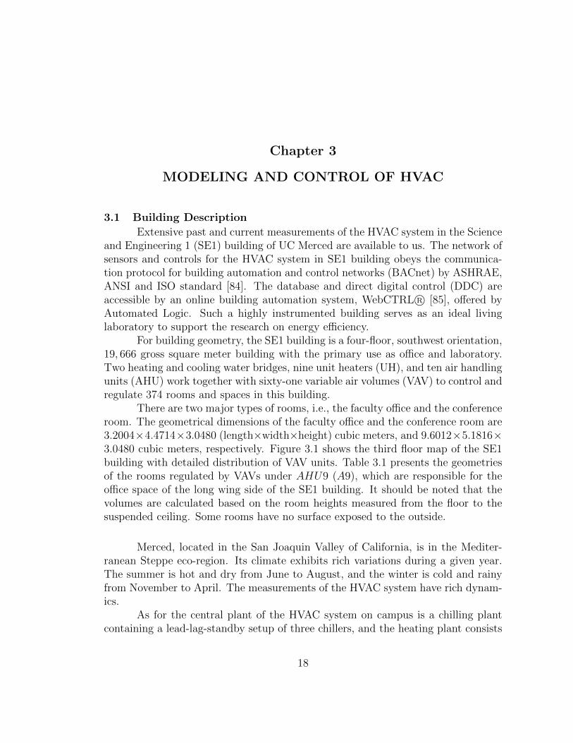
There are two major types of rooms, i.e., the faculty office and the conferenceroom. The geometrical dimensions of the faculty office and the conference room are3.2004×4.4714×3.0480 (length×width×height) cubic meters, and 9.6012×5.1816×3.0480 cubic meters, respectively. Figure 3.1 shows the third floor map of the SE1building with detailed distribution of VAV units. Table 3.1 presents the geometriesof the rooms regulated by VAVs under AHU9 (A9), which are responsible for theoffice space of the long wing side of the SE1 building. It should be noted that thevolumes are calculated based on the room heights measured from the floor to thesuspended ceiling. Some rooms have no surface exposed to the outside.

Merced, located in the San Joaquin Valley of California, is in the Mediter-ranean Steppe eco-region. Its climate exhibits rich variations during a given year.The summer is hot and dry from June to August, and the winter is cold and rainyfrom November to April. The measurements of the HVAC system have rich dynam-ics.

As for the central plant of the HVAC system on campus is a chilling plantcontaining a lead-lag-standby setup of three chillers, and the heating plant consists

18

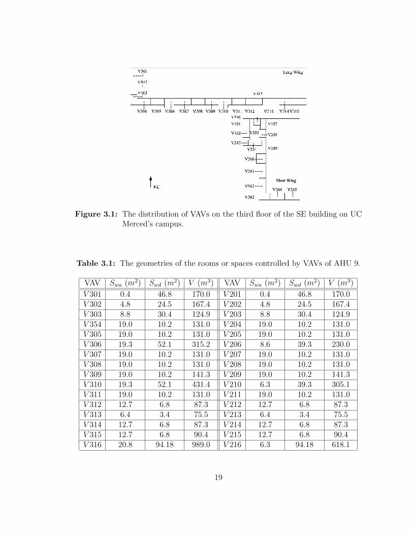
Figure 3.1: The distribution of VAVs on the third floor of the SE building on UCMerced’s campus.

Table 3.1: The geometries of the rooms or spaces controlled by VAVs of AHU 9.

VAV Swa (m2) Swd (m2) V (m3) VAV Swa (m2) Swd (m2) V (m3)

V 301 0.4 46.8 170.0 V 201 0.4 46.8 170.0V 302 4.8 24.5 167.4 V 202 4.8 24.5 167.4V 303 8.8 30.4 124.9 V 203 8.8 30.4 124.9V 354 19.0 10.2 131.0 V 204 19.0 10.2 131.0V 305 19.0 10.2 131.0 V 205 19.0 10.2 131.0V 306 19.3 52.1 315.2 V 206 8.6 39.3 230.0V 307 19.0 10.2 131.0 V 207 19.0 10.2 131.0V 308 19.0 10.2 131.0 V 208 19.0 10.2 131.0V 309 19.0 10.2 141.3 V 209 19.0 10.2 141.3V 310 19.3 52.1 431.4 V 210 6.3 39.3 305.1V 311 19.0 10.2 131.0 V 211 19.0 10.2 131.0V 312 12.7 6.8 87.3 V 212 12.7 6.8 87.3V 313 6.4 3.4 75.5 V 213 6.4 3.4 75.5V 314 12.7 6.8 87.3 V 214 12.7 6.8 87.3V 315 12.7 6.8 90.4 V 215 12.7 6.8 90.4V 316 20.8 94.18 989.0 V 216 6.3 94.18 618.1

19

of three, dual fuel boilers. The pump speeds of both plants are modulated byPID controls to maintain differential pressures at discharge. To building level sub-systems, the AHU units apply logic and PID controls to regulate the supply fanvariable-frequency drive (VFD), return fan VFD, adjust the damper position ofchilling water and supply air temperature. These control loops maintain the ductpressure, return fan discharge pressure, and supply air temperature according to theset point. The VAV units implement two separate control loops, i.e., the coolingloop and the heating loop, to keep the temperature at set point. Both of the loopsapply PI controls with three operational modes: heating, cooling, and deadband.In summer, the heating loop is barely used and the cooling valve is always open.

The PID controls are localized and are actually involved in one another bythermodynamics. However, the relationship of the inputs, outputs, parameters, anddisturbance of each control loop are not explicit from WebCTRL R©. Thus, for amore global and intelligent control strategy, we need to build dynamical models forthis HVAC process.

3.2 Mathematical Model

3.2.1 Introduction

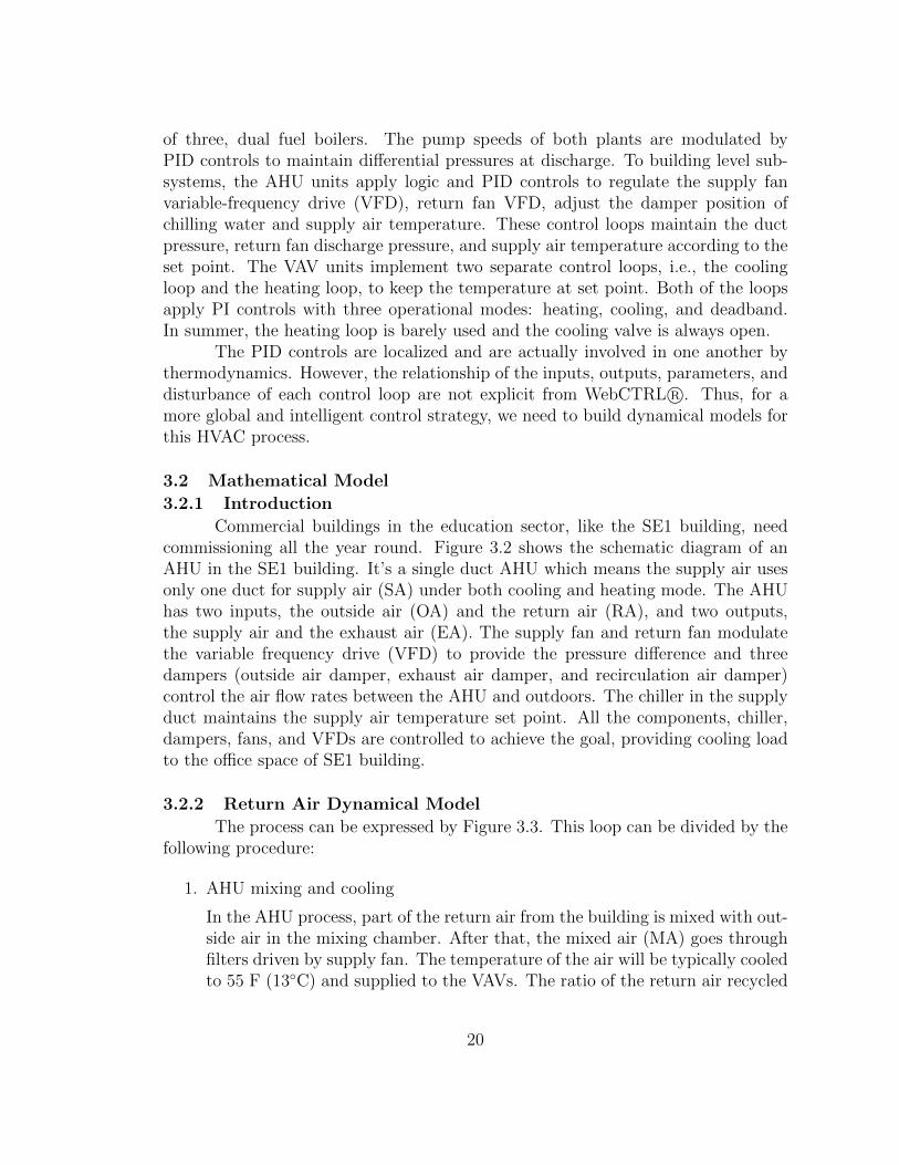
Commercial buildings in the education sector, like the SE1 building, needcommissioning all the year round. Figure 3.2 shows the schematic diagram of anAHU in the SE1 building. It’s a single duct AHU which means the supply air usesonly one duct for supply air (SA) under both cooling and heating mode. The AHUhas two inputs, the outside air (OA) and the return air (RA), and two outputs,the supply air and the exhaust air (EA). The supply fan and return fan modulatethe variable frequency drive (VFD) to provide the pressure difference and threedampers (outside air damper, exhaust air damper, and recirculation air damper)control the air flow rates between the AHU and outdoors. The chiller in the supplyduct maintains the supply air temperature set point. All the components, chiller,dampers, fans, and VFDs are controlled to achieve the goal, providing cooling loadto the office space of SE1 building.

3.2.2 Return Air Dynamical Model

The process can be expressed by Figure 3.3. This loop can be divided by thefollowing procedure:

1. AHU mixing and cooling

In the AHU process, part of the return air from the building is mixed with out-side air in the mixing chamber. After that, the mixed air (MA) goes throughfilters driven by supply fan. The temperature of the air will be typically cooledto 55 F (13◦C) and supplied to the VAVs. The ratio of the return air recycled

20

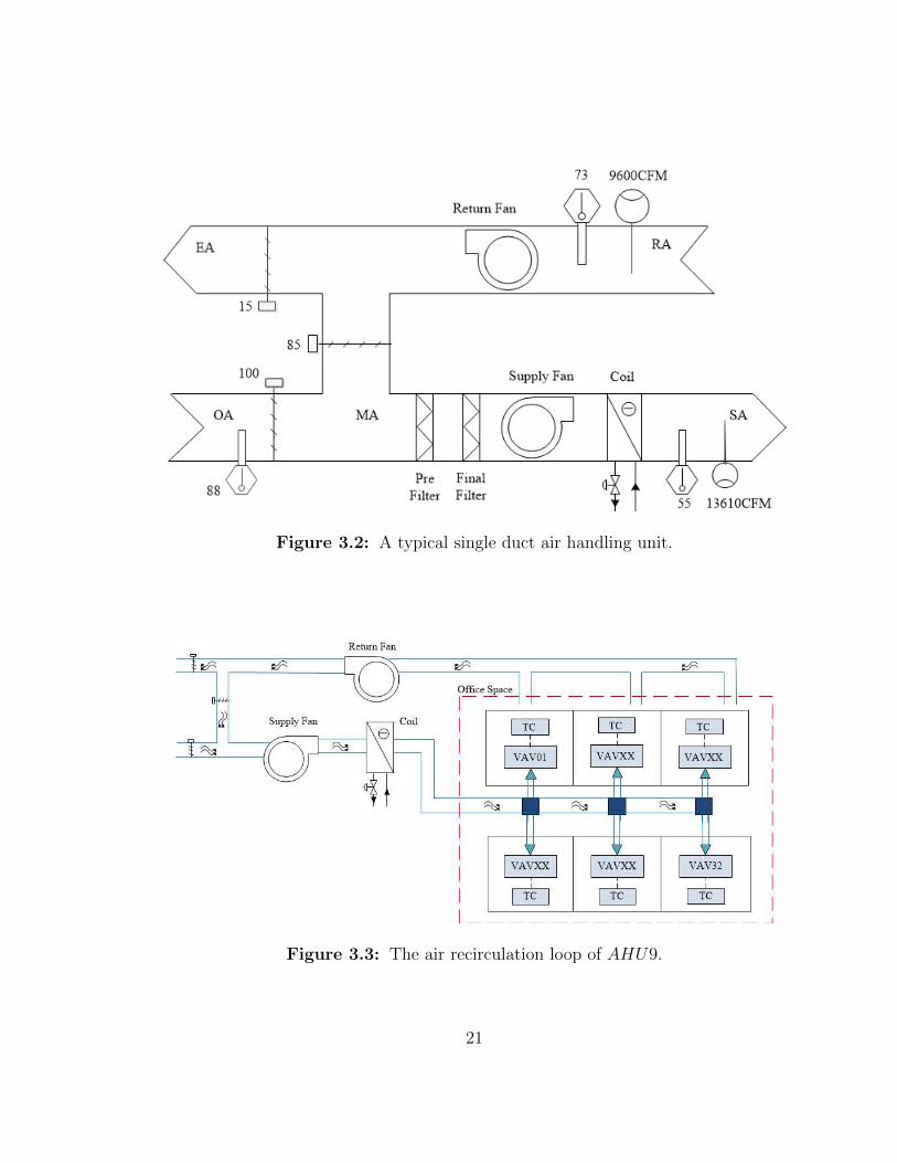
Figure 3.2: A typical single duct air handling unit.

Figure 3.3: The air recirculation loop of AHU9.

21

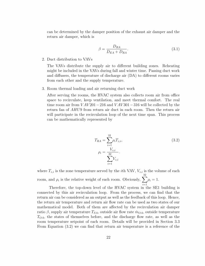
can be determined by the damper position of the exhaust air damper and thereturn air damper, which is

β =DRA

DEA +DRA

. (3.1)

2. Duct distribution to VAVs

The VAVs distribute the supply air to different building zones. Reheatingmight be included in the VAVs during fall and winter time. Passing duct workand diffusers, the temperature of discharge air (DA) to different rooms variesfrom each other and the supply temperature.

3. Room thermal loading and air returning duct work

After serving the rooms, the HVAC system also collects room air from officespace to recirculate, keep ventilation, and meet thermal comfort. The realtime room air from V AV 201−216 and V AV 301−316 will be collected by thereturn fan of AHU9 from return air duct in each room. Then the return airwill participate in the recirculation loop of the next time span. This processcan be mathematically represented by

TRA =32∑i=1

ρiTz,i, (3.2)

ρi =Vz,i

32∑i=1

Vz,i

.

where Tz,i is the zone temperature served by the ith VAV, Vz,i is the volume of each

room, and ρi is the relative weight of each room. Obviously,32∑i=1

ρi = 1.

Therefore, the top-down level of the HVAC system in the SE1 building isconnected by this air recirculation loop. From the process, we can find that thereturn air can be considered as an output as well as the feedback of this loop. Hence,the return air temperature and return air flow rate can be used as two states of ourmathematical model. Both of them are affected by the recirculation air damperratio β, supply air temperature TSA, outside air flow rate mOA, outside temperatureTOA, the states of themselves before, and the discharge flow rate, as well as theroom temperature setpoint of each room. Details will be provided in Section 3.3From Equation (3.2) we can find that return air temperature is a reference of the

22

18 20 22 24 2670

71

72

73

74

75

Days (May)

Tem

perature

(F)

TRA

Tzone

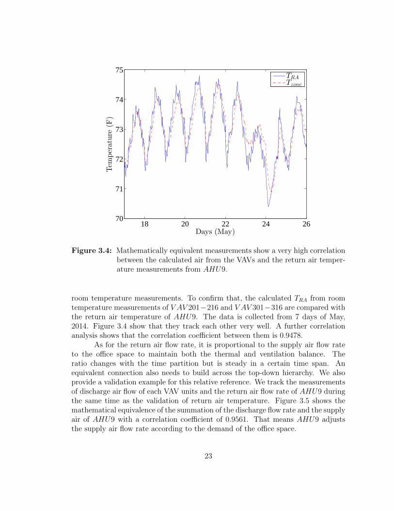
Figure 3.4: Mathematically equivalent measurements show a very high correlationbetween the calculated air from the VAVs and the return air temper-ature measurements from AHU9.

room temperature measurements. To confirm that, the calculated TRA from roomtemperature measurements of V AV 201−216 and V AV 301−316 are compared withthe return air temperature of AHU9. The data is collected from 7 days of May,2014. Figure 3.4 show that they track each other very well. A further correlationanalysis shows that the correlation coefficient between them is 0.9478.

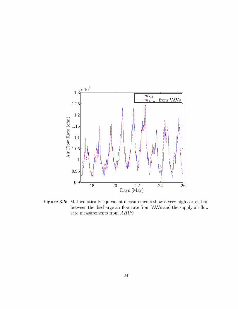
As for the return air flow rate, it is proportional to the supply air flow rateto the office space to maintain both the thermal and ventilation balance. Theratio changes with the time partition but is steady in a certain time span. Anequivalent connection also needs to build across the top-down hierarchy. We alsoprovide a validation example for this relative reference. We track the measurementsof discharge air flow of each VAV units and the return air flow rate of AHU9 duringthe same time as the validation of return air temperature. Figure 3.5 shows themathematical equivalence of the summation of the discharge flow rate and the supplyair of AHU9 with a correlation coefficient of 0.9561. That means AHU9 adjuststhe supply air flow rate according to the demand of the office space.

23

18 20 22 24 260.9

0.95

1

1.05

1.1

1.15

1.2

1.25

1.3x 10

4

Days (May)

Air

Flow

Rate(cfm

)

˙mSA

˙mDisch from VAVs

Figure 3.5: Mathematically equivalent measurements show a very high correlationbetween the discharge air flow rate from VAVs and the supply air flowrate measurements from AHU9

24

Now we can try to derive the mathematical model from the HVAC back-ground. Typically a first order plus time delay (FOPTD) is used to represent anHVAC process [86] such as

G(s) =X(s)

U(s)=

K

Ts+ 1exp(−Ls), (3.3)

where K is the process gain and L represents the time-delay. The input and outputlogged until the process enters a new steady state gain. The parameter identificationof this model is easy but might be sensitive to measurement noise and determined bycomplex manipulated variables. Additionally, FOPTD works better for componentsrather than a multi-agent process. For multiple control inputs and state variables,and systems with disturbance, we consider the ARMAX model

x(n+ 1) =

NP∑i=0

a(i)x(n− i) +

NC∑i=0

b(i)u(n− i) + cw(n), (3.4)

where x(n) is the state variable,u(n) is the control input and w(n) is the disturbance.The model is explicit for control design. Take the return air temperature model asan example:

TRA(n+ 1) =

NP∑i=0

at(i)TRA(n− i) +

NC∑i=0

(bt,1(i)β(n− i) + bt,2(i)TSA(n− i) (3.5)

+ bt,3(i)mOA(n− i)) + ctTOA(n).

This model is easy to implement into a controller design. TRA is the statebeing observed, β, TSA(n−i) and mOA are manipulated variables, and TOA representsthe real time climate treated as a disturbance since it cannot be controlled. Largescale of measurements from AHU, VAVs, and outside air condition are available todetermine the model parameters. This results in a collection of coefficients at, bt,1,bt,2 ,bt,3 and ct. It should be noted that when the length of the prediction horizionis 1 or 2, the order of this ARMAX model is consistent with the thermodynamiclaws.

3.2.3 Energy Model

The energy consumption of an AHU in Figure 3.2 consists mainly of thecooling load of the water chiller and electricity usage of both the supply fan and thereturn fan.

EnAHU = EnCW +WF t, (3.6)

WF = WSF +WRF .

25

The water coil needs to cover the energy required to cool down mixed air tothe set point of the supply air temperature. It is assumed and so it is in Mercedthat the outside air is very dry, where the dew point is less than 55 F (13C). Thatmeans no latent heat is lost and only the sensible cooling load is considered duringthe cooling process. In the continuity condition, mMA = mSA, therefore the energyconsumption of the water chiller can be expressed as

EnCW = cpmSA(TMA − TSA). (3.7)

Before passing through the supply fan, the mixed air temperature is fixed bythe combination of outside air and recirculated air in the mixing chamber. If TMA

is above saturation line, the moisture in the air won’t condensate, and the flow rateand temperature balance during an air economizer cycle is

mSA = mOA + βmRA, (3.8)

cpmOATOA + βcpmRATRA = cpmSATMA. (3.9)

Combining Equation (3.7), (3.8) and (3.9), the cooling load can be expressedas

EnCW = cpmSATMA − cpmSATSA, (3.10)

= cpmOATOA + βcpmRATRA − cp(mOA + βmRA)TSA,

= cpmOA(TOA − TSA) + βcpmRA(TRA − TSA).

Otherwise, the power usage of the supply and return fans follows the affinitylaw. P is proportional to the third power of the flow rate m, as shown in Equation(3.11).

WF = WSF +WRF , (3.11)

= WSF,ref (mSA

mSA,ref

)3 +WRF , ref(mRA

mRA,ref

)3.

The reference power and flow rate are calculated from real operation of HVACsystem in the SE1 building.

In summary, the energy consumption of AHU can be expressed as

EnAHU = cpmOA(TOA − TSA) + βcpmRA(TRA − TSA) (3.12)

+WSF,ref (mSA

mSA,ref

)3 +WRF,ref (mRA

mRA,ref

)3.

26

3.3 Control Formulation

3.3.1 HVAC Background

A stereotype AHU is multi-functional. The primary purposes include distri-bution of supply air to the building zone at a set point value, keeping the building instatic pressure. As described in Section 3.2.2, AHU9 in the SE1 building is runningin an enconomizer cycle, and the transient time is short compared to the steadystate of each time span. For dampers, the outside air flow rate, and the supply airtemperature, local PID control is applied to every single component with only a sim-ple link to each other [12]. However, to minimize energy consumption and optimizethermal comfort, the traditional control might not yield the optimal solution. In thissection, an energy efficient and multi-objective MPC control strategy that considersventilation and thermal load is introduced based on the same control variables inthe original local PID control. The advantages of applying MPC include:

• A physical-based inherent connection between components in the AHU, andconsiders cross-level constraints in the whole HVAC system of the SE1building.

• The controller is designed to be online, receding state prediction andfuture optimal control inputs calculation.

• The impact of measurement noise and nonlinearities is reduced by dataregression and time domain integration.

• The algorithm is based on WebCTRL R©, and is easily implemented intobuilding automation systems.

3.3.2 Model Predictive Control

For comparison, the same manipulated variables are chosen as the originallocal PID control: the recirculation air damper ratio β, the supply air temperatureTSA and the outside air flow rate mOA. The model of AHU9 in the SE1 buildingincludes the control inputs and can be represented by the model proposed in Section3.2.2. For simplicity, the prediction horizon is set to be N and the control horizonis used as N − 1:

x(k + 1) =N∑i=0

A(i)x(k − i) +N−1∑i=0

B(i)u(k − i) + Cw(k), (3.13)

where x(k) = [TRA(k), mRA(k)]T , u(k) = [β(k), TSA(k), mOA(k)]T , w(k) = TOA(k).Note that ∆u(k) = [∆β(k),∆TSA(k),∆mOA(k)]T , rather than u(k), is commonlycalculated in realistic computation, and ∆u(k) = u(k)− u(k − 1).

Then the objective function can be expressed at every sample time k:

27

J =N∑j=0

(Q1j |TRA,ref (k + j)− TRA(k + j | k)|2 (3.14)

+Q2j |mRA,ref (k + j)− mRA(k + j | k)|2)

+N−1∑j=0

(EnAHU(k + j | k) +Q3j |mSA,ref (k + j)− mSA(k + j | k)|2

+R1j |∆β(k + j | k)|2 +R2j |∆TSA(k + j | k)|2

+R3j |∆mOA(k + j | k)|2),

where EnAHU(k) follows the structure of Equation (3.12), TRA,ref (k) and mRA,ref (k)is the designed set point from historic data as reference of zone temperature andventilation level of SE1 building It should be noted that the supply air flow ratemSA,ref (k) is also an observable variable. It indicates the demands of fresh airamount. Also, its product multiplying to TRA,ref (k), the reference of the roomtemperatures set point, can present cooling load demand of the building. The supplyair flow rate mSA,ref (k) can be represented as Equation (3.8).

To find optimal control inputs, the gradient-based Lagrangian solution methodare introduced to the objective function. The mathematical models of the statesTRA(k) and mRA(k) serve as constraints of the dynamical behavior of HVAC sys-tem. They are linked to the original objective function with Lagrangian Multipliers.Thus, the updated objective function can be defined as:

J∗ = J +N∑j=1

λj(TRA(k + j | k)− f(TRA(k + j − 1 | k),∆u(k + j − 1 | k))) (3.15)

+ µj(mRA(k + j | k)− g(mRA(k + j − 1 | k),∆u(k + j − 1 | k))).

where f(TRA(k+j−1 | k),∆u(k+j−1 | k)) and g(mRA(k+j−1 | k),∆u(k+j−1 | k))are referred to the ARMAX models in Equation 3.13.

The optimization problem is shown from Equations (3.16) to (3.17g):

min∆u

J∗(x,∆u, λ, µ), (3.16)

subject to the following constraints:

28

βmin ≤ β(k + j | k) ≤ βmax, (3.17a)

TSA,min ≤ TSA(k + j | k) ≤ TSA,max, (3.17b)

mOA,min ≤ mOA(k + j | k) ≤ mOA,max, (3.17c)

∆βmin ≤ ∆β(k + j | k) ≤ ∆βmax, (3.17d)

∆TSA,min ≤ ∆TSA(k + j | k) ≤ ∆TSA,max, (3.17e)

∆mOA,min ≤ ∆mOA(k + j | k) ≤ ∆mOA,max, (3.17f)

TRA(k + j | k) = f(TRA(k + j − 1 | k),∆u(k + j − 1 | k)), (3.17g)

mRA(k + j | k) = g(mRA(k + j − 1 | k),∆u(k + j − 1 | k)). (3.17h)

The control inputs in this study have different physical meanings. β is therecirculation air damper ratio; it is easy to find if the return air damper is fully open(DRA = 1) and the exhaust air damper is fully closed (DEA = 0) at the same time.When this occurs β = 1, which means all the return air is recycled for the next timespan of air supply. Otherwise, when the return air damper is fully closed (DRA = 0)and the exhaust air damper is fully open (DEA = 1), β = 0. In this situation, thereturn air is all relieved and the supply air is provided by fresh air. However, tokeep the building static pressure’s balanced and make sure there is enough fresh airfor supply, these two extreme cases would not happen. The physical lower boundof DEA and DRA is set to 15% and 12% respectively. The upper bounds are both100%, fully open. Therefore the range of β can be shown as:

βmin =DRA,min

DEA,max +DRA,min

≈ 11%, (3.18)

βmax =DRA,max

DEA,min +DRA,max

≈ 87%.

To determine the bounds of TSA, the designed supply air temperature TSA,d of55 F (13 C) is used as the lower bound TSA,min. This is a conventional temperaturefor supply air in HVAC systems. However, if the dew point of the outside air isbelow 55 F, the latent cooling load would not exist. In this case, no saturated steamwill condensate [66]. Therefore the TSA can be not limited and higher set pointcan be used for reducing the AHU’s energy consumption. It should be noted thatTSA,max is cooling load demand generated by occupants and devices in the buildingzone area.

For the outside air flow rate mOA, the minimum outside air flow rate is 3000cubic feet per minute (cfm), which is determined by the BAS of the SE1 building.

29

This number is set according to the requirement of the outdoor air needed per personin office buildings from ASHRAE Standard 62.1 [87]. The upper bound value of theoutside air flow rate cannot exceed that of the supply air flow rate. The limitationsof mOA can be shown as:

mOA,min = 3000 cfm, (3.19)

mOA,max = mSA,d.

In addition, the reference trajectory in this approach, TRA,ref , mRA,ref andmSA,ref need to be determined for the objective function. As mentioned in Section3.2.2, the return air temperature of AHU9 is a weighted average from room tem-perature in the office space of the SE1 building. Thus, the set point of each roomtemperature can be a reference for the state of return air temperature, that is,

TRA,ref =32∑i=1

ρiTset,i, (3.20)

where Tset,i is the set point of room temperature in each zone and ρi is the weightof each zone. Similarly, the reference of supply air reference can be expressed as thesummation of the set point of discharge air flow rate in each zone,

mSA,ref =32∑i=1

mset,i (3.21)

And the return air flow rate reference is proportional to the supply air reference,

mRA,ref = αmSA,ref (3.22)

The ratio α is calculated from the designed set point and the historic data fromsummer 2014. Since we use historic air flow rates as reference, the effect of fanpowers can be neglected according to the affinity law.

After the parameter identification, now we can apply the gradient to theobjective function. Take prediction horizon p = 2, control horizon m = p − 1 = 1as an example:

∂J∗

∂x1(k+2|k)∂J∗

∂x2(k+2|k)∂J∗

∂∆u1(k|k)∂J∗

∂∆u2(k|k)∂J∗

∂∆u3(k|k)∂J∗

∂λ(k+2)∂J∗

∂µ(k+2)

=

∂J∗

∂TRA(k+2|k)∂J∗

∂mRA(k+2|k)∂J∗

∂∆β(k|k)∂J∗

∂∆TSA(k|k)∂J∗

∂∆mOA(k|k)∂J∗

∂λ(k+2)∂J∗

∂µ(k+2)

= 0, (3.23)

30

where

∂J∗

∂TRA(k + 2 | k)= 2Q1(TRA(k + 2 | k)− TRA,ref (k + 2)) + λ(k + 2), (3.24)

∂J∗

∂mRA(k + 2 | k)= 2Q2(mRA(k + 2 | k)− mRA,ref (k + 2)) + µ(k + 2), (3.25)

∂J∗

∂∆β(k | k)= cpmRA(k + 1 | k)(TRA(k + 1 | k)− TSA(k)−∆TSA(k | k)) (3.26)

+ 2Q3mRA(k + 1 | k)(mRA(k + 1 | k)(β(k) + ∆β(k | k))

+ (mOA(k) + ∆mOA(k | k))− mSA,ref (k + 1))

+ 2R1∆β(k | k)− bt,1λ(k + 2)− bf,1µ(k + 2),

∂J∗

∂∆TSA(k | k)= −cp(mOA(k) + ∆mOA(k | k) (3.27)

+ (β(k) + ∆β(k | k))mRA(k + 1 | k))

+ 2R2∆TSA(k | k)− bt,2λ(k + 2)− bf,2µ(k + 2),

∂J∗

∂∆mOA(k | k)= cp(Toa(k + 1)− (TSA(k) + ∆TSA(k | k)) (3.28)

+ 2Q3(mOA(k) + ∆mOA(k | k)

+ (β(k) + ∆β(k | k))mRA(k + 1 | k))

+ 2R3∆mOA(k | k)− bt,3λ(k + 2)− bf,3µ(k + 2),

∂J∗

∂λ(k + 2)= TRA(k + 2 | k)− (atTRA(k + 1 | k) + bt,1(β(k) + ∆β(k | k))

+ bt,2(TSA(k) + ∆TSA(k | k)) + bt,3(mOA(k) + ∆mOA(k | k)) (3.29)

+ ctToa(k + 1)),

∂J∗

∂µ(k + 2)= mRA(k + 2 | k)− (afmRA(k + 1 | k) + bf,1(β(k) + ∆β(k | k))

+ bf,2(TSA(k) + ∆TSA(k | k)) + bf,3(mOA(k) + ∆mOA(k | k)) (3.30)

+ cfToa(k + 1)),

Actually Equations (3.29) and (3.30) are the state equations that predict the valueof the sates at the time interval k + 2. They serve as the dynamical constraints

31

inside the optimization problem. If we put all the constants on the right-hand-side,the equations can be represented in the matrix form

Q 0 I2

0 R BT

I2 B 0

TRA(k + 2 | k)mRA(k + 2 | k)

∆β(k | k)∆TSA(k | k)∆mOA(k | k)

λµ

= d, (3.31)

where

Q = 2

[Q1 00 Q2

], (3.32)

R =

−2δm2RA(k + 1 | k)− 2R1 cpmRA(k + 1 | k) −2Q3mRA(k + 1 | k)

−cpmRA(k + 1 | k) −2R2 cp−2Q3mRA(k + 1 | k) cp −2δ − 2R3

,(3.33)

B =

[bt,1 bt,2 bt,3bf,1 bf,2 bf,3

]. (3.34)

And the right-hand-side is a vector of constant, which is

d = [d1, d2, d3, d4, d5, d6, d7]T , (3.35)

whered1 = Q1TRA,ref (k + 2), (3.36)

d2 = Q2mRA,ref (k + 2) (3.37)

d3 = cpmRA(k + 1 | k)TRA(k + 1 | k) (3.38)

+ 2Q3mRA(k + 1 | k)(mOA(k | k) + β(k | k)mRA(k + 1 | k)

− mSA,ref (k + 1)),

d4 = −cp(mOA(k | k) + β(k | k)mRA(k + 1 | k)), (3.39)

d5 = cp(Toa(k + 1)− TSA(k | k)) (3.40)

+ 2Q3(mOA(k | k) + β(k | k)mRA(k + 1 | k)

− mSA,ref (k + 1)),

d6 = atTRA(k + 1 | k) + bt,1β(k | k) + bt,2TSA(k | k) + bt,3mOA(k | k) (3.41)

+ ctToa(k + 1),

32

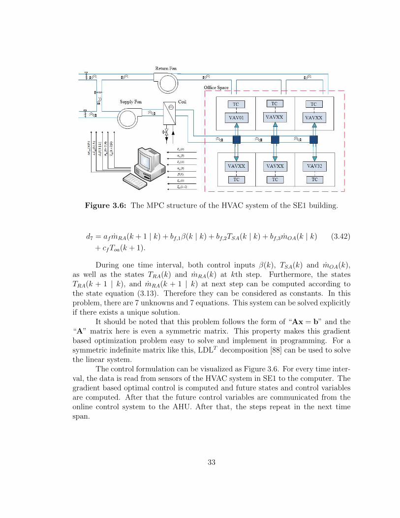
Figure 3.6: The MPC structure of the HVAC system of the SE1 building.

d7 = afmRA(k + 1 | k) + bf,1β(k | k) + bf,2TSA(k | k) + bf,3mOA(k | k) (3.42)

+ cfToa(k + 1).

During one time interval, both control inputs β(k), TSA(k) and mOA(k),as well as the states TRA(k) and mRA(k) at kth step. Furthermore, the statesTRA(k + 1 | k), and mRA(k + 1 | k) at next step can be computed according tothe state equation (3.13). Therefore they can be considered as constants. In thisproblem, there are 7 unknowns and 7 equations. This system can be solved explicitlyif there exists a unique solution.

It should be noted that this problem follows the form of “Ax = b” and the“A” matrix here is even a symmetric matrix. This property makes this gradientbased optimization problem easy to solve and implement in programming. For asymmetric indefinite matrix like this, LDLT decomposition [88] can be used to solvethe linear system.

The control formulation can be visualized as Figure 3.6. For every time inter-val, the data is read from sensors of the HVAC system in SE1 to the computer. Thegradient based optimal control is computed and future states and control variablesare computed. After that the future control variables are communicated from theonline control system to the AHU. After that, the steps repeat in the next timespan.

33

Chapter 4

NUMERICAL RESULTS

4.1 Mathematical Model Evaluation

4.1.1 Data Preprocessing

Measurements from thirty VAVs and AHU9 are available for the developmentof the ARMAX model. From May 1 to July 31, 2014, measurements of temperatureTOA, TMA, TSA and TRA; air flow rates mOA, mRA, and mSA; damper positions DOA,DRA and DEA; fan power WSF and WRF from AHU9, room temperature Trm and itsset point of Trm,sp, the discharge air flow rate mdis and its demand set point mdis,sp

from each affiliated VAV have been collected over 26 days with a sampling intervalof fifteen minutes, resulting in 2, 496 samples. The BAS of the SE1 building appliesa different operation strategy during the day from 7:30am to 1am, and during thenight from 1am to 7:30am. During the day time, the HVAC system shows a diversedynamics and more control efforts are imposed since the internal thermal load ishigher. It’s called occupied mode for WebCTRL R©. The operation mode in thenight is called unoccupied mode. Most of the occupants work during the day. Thedifference in occupancy between weekdays and weekends is insignificant. We dividethe data by day and night with the same time partition and focus on the data thatfalls under occupied mode.

4.1.2 Data Smoothing

The measurements from HVAC systems have noise. In the SE1 building,the measurements are read from sensors and then linked to the BAS. Noise is alsopart of the sensor readings and not good for the parameter identification of linearregression. The sensor location, and lack of routine maintenance affect the accuracyof the measurements. Sensor noise in HVAC systems are regarded as white randomnoise [89]. However, the estimation of bias is sensitive to the measurements scale[90]. The real bias is not easy to find. Thus, a smoothing method, the Savitzky-Golay filter [91], is used for denoising in flow rate measurements of the SE1 buildingTypical filters, like the plain FIR filter, might remove useful high-frequency signalsin measurements [92]. Savitzky-Golay filter, also known as a polynomial smoothing,or least-squares smoothing filter can preserve better high-frequency information.The polynomial fitting is equivalent to discrete convolution across a moving window

34

on the time domain. It is a low-pass filter that maintains the shape and heightof waveform peaks [93]. These properties are beneficial to the HVAC system’smeasurements noise reduction. For flow rate measurements, the peaks representthe high demand of the cooling load of the building. Also, the HVAC system’sdynamic is relatively slow compared to the sampling interval and the measurementsare periodic in shape day by day. The preservation of the peak and shapes can helpus save the useful content for modeling while reducing noise.

Consider a measurement x in a group with M sampling numbers. The datax(n) at the center of a moving window is set as n = 0. It is the target filter data.All the points of x(n) in this zone can be approximated with a polynomial as

p(n) =N∑k=0

aknk, (4.1)

where k is the order of each term and N is the highest order of the polynomial. Thesmoothed output value y(0) is obtained by evaluating p(n) at n = 0, which is

y(0) = p(0) = a0. (4.2)

That means, the value of smoothed data is equal to the 0th order polynomial value.To find a0, the optimal coefficients need to be calculated. The optimal coefficientscan be found by minimizing the mean squared error (MSE) of Equation (4.1). forthe points in the zone,

εN =

M−12∑

n=−M−12

(p(n)− x(n))2

=

M−12∑

n=−M−12

(N∑k=0

aknk − x(n))2. (4.3)

Thus, differentiation is applied to εN in Equation (4.3) with respect to each sampleof the N+1 unknown coefficients and setting the corresponding derivatives equal to0. Thus, for i = 0, 1, . . . , n,

∂εN∂ai

=

M−12∑

n=−M−12

2ni(N∑k=0

aknk − x(n)),

which can be rewritten as

N∑k=0

(

M−12∑

n=−M−12

nk+i)ak =

M−12∑

n=−M−12

nix(n). (4.4)

35

To solve Equation (4.4), a M by N + 1 matrix A can be defined as A = {ni}for i = 0, 1, . . . , n, and a N + 1 by N + 1 symmetric matrix B = ATA. ThusEquation 4.4 can be represented as

Ba = ATAa = ATx, (4.5)

where a = [a0, a1, . . . , aN ]T , and x = [x(−M−12

), . . . , x(−1), x(0), x(1), . . . , x(M−12

)].Therefore, the solution of the polynomial coefficient can be written as

a = (ATA)−1ATx = Hx. (4.6)

Recall that from the output of Equation (4.2) only a0 is need for approximation.Thus, only the first row of H matrix is needed to compute a0. Using h0,m to denotethe elements of the first row of the H matrix, the smoothed data can be representedas

y(0) = a0 =

M−12∑

m=−M−12

h0,mx(m), (4.7)

where it is obvious that all the data in the zone is used to smooth the value targetpoint.

In the design of Savitzky-Golay filter, the selection of M and N affects theresult of the smoothed data. A too large N close to M can lead to a badly condi-tioned H matrix. A huge window size of M can result in excessive information fromthe past and future. For our problem, M is chosen as 5 since it only contains thecontent of points from n − 2 to n + 2 for the nth measurement. This is consistentwith the length of the prediction horizon of our approach. The highest polynomialorder N is set to 3. Therefore, the smoothed data at the nth step can be representedas

y(n) =1

35(−3x(n− 2) + 12x(n− 1) + 17x(n) + 12x(n+ 1)− 3x(n+ 2)), (4.8)

where the coefficients are calculated from the first row of the 4 by 5 H matrix.Figure 4.1 shows the smoothing effect of the Savitzky-Golay filter on the

return air flow rate of AHU9 in the SE1 building. The data is sampled during 26days in May, 2014. The high-frequency oscillation of the original data is reduced.Meanwhile, the shape and peaks of the data are preserved. The average value ofthe smoothed data remains the same as the raw data, 7, 362 cubic meter per minute(cfm). This proves it is feasible to obtain smoothed data for modeling and control.The comparison of the model validation with both the raw data and the smootheddata will be provided in Section 4.1.4.

However, the Savitzky-Golay filter cannot be implemented to real time sinceit needs future measurements. A low-pass filter, such as the Butterworth filter [94] is

36

0 5 10 15 20 254000

6000

8000

10000

12000

Raw Data

˙m

RA(cfm

)

0 5 10 15 20 254000

6000

8000

10000

12000

Smoothed Data

Days (May)

˙m

RA(cfm

)

Figure 4.1: Comparison of the raw data (upper subplot) with the smoothed databy the Savitzky-Golay filter (lower subplot) in May, 2014.

37

used in real time data smoothing here. This filter has a property of a maximally flatmagnitude in the passband [95]. The design of Butterworth filter can be specifiedby two parameters, the order of filter n and the cutoff frequency ωc [96].

The Butterworth filter is widely used for data smoothing in different fields,such as handwriting movement [97], inertia navigation system [98] and biomechanics[99]. It has a sufficient accuracy with a low programming effort. However, in digitalimplementation, the phase delay introduced by this filter has to be considered. Thedynamics of the HVAC system is slow. A small time delay is acceptable. An orderof filter n = 2 and a normalized cutoff frequency ωc = 0.5 are selected. The resultingdigital filter brings one step time delay. It should be noted that the second order isalso consistent to the prediction horizon as well as the order of the Savitzky-Golayfilter considered earlier.

The transfer function of a second order Butterworth filter can be written as

H(s) =1

( sωc

)2 + 1.4142 sωc

+ 1. (4.9)

The bilinear transform is used to convert it to digital time domain

s ≈ 2

T

1− z−1

1 + z−1, (4.10)

where T is the sample period. We define K , 2T

. This results in the digitalButterworth filter form as

Hd(z) =1 + 2z−1 + z−2

((Kωc

)2 + 1.4142Kωc

+ 1) + (2− 2(Kωc

)2)z−1 + ((Kωc

)2 − 1.4142Kωc

+ 1)z−2

≈ 0.2929 + 0.5858z−1 + 0.2929z−2

1 + 0.1716z−2. (4.11)

The difference equation of the smoothed data y(n) at the nth step from raw mea-surement x(n) can be represented as

y(n) = 0.2929x(n) + 0.5858x(n− 1) + 0.2929x(n− 2)− 0.1716y(n− 2). (4.12)

The example of the Butterworth data smoothing is shown in Figure 4.2. Thehigh frequency noise has been reduced, meanwhile the phase delay is reasonablysmall.

4.1.3 Model Validation

We identify the collection of coefficients a, b1, b2 ,b3 and c with the methodof least squares by using Equation (3.13). The least square solution of those threeparameters is obtained by using the backslash operator in MATLAB [100]. The

38

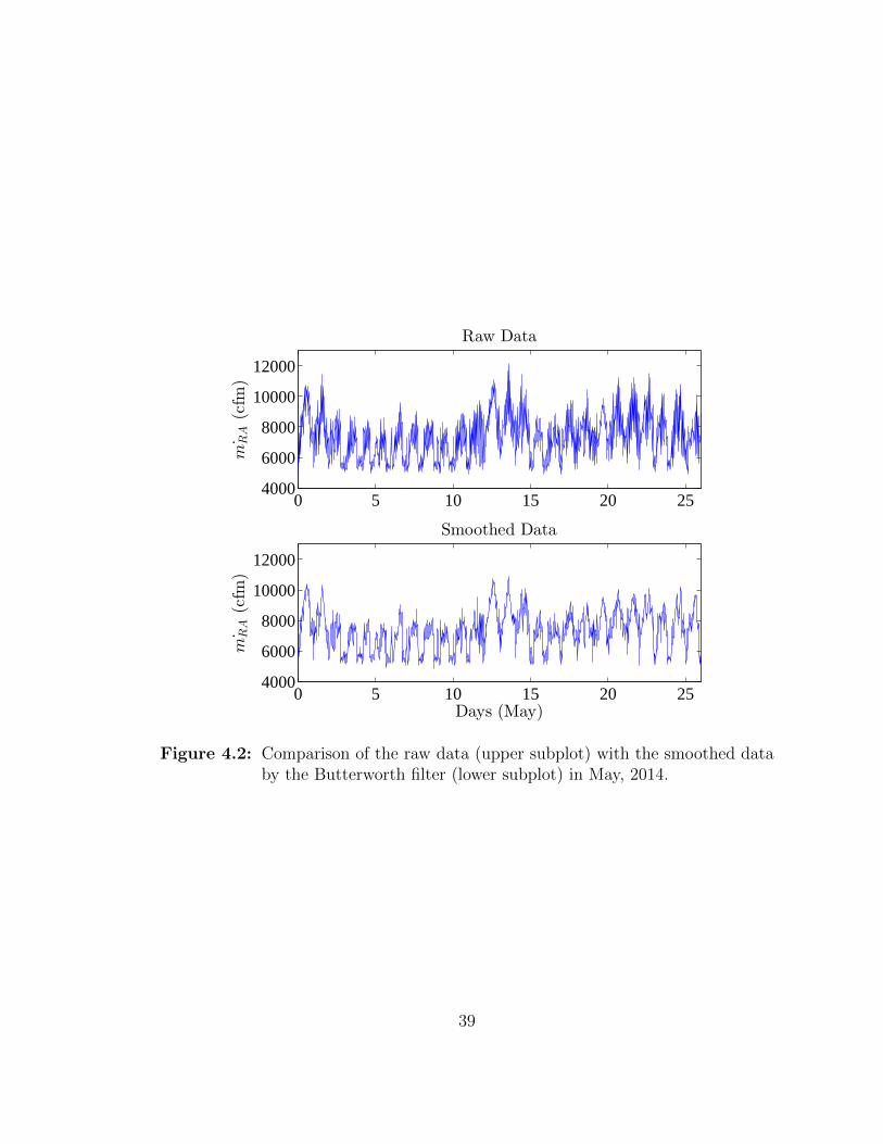
0 5 10 15 20 254000

6000

8000

10000

12000

Raw Data

˙m

RA(cfm

)

0 5 10 15 20 254000

6000

8000

10000

12000

Smoothed Data

Days (May)

˙m

RA(cfm

)

Figure 4.2: Comparison of the raw data (upper subplot) with the smoothed databy the Butterworth filter (lower subplot) in May, 2014.

39

method to numerically determine the optimal number of samples for parameteridentification has been discussed in the previous work of our group [50,53].

To validate the model, we first select a metric for evaluating the accuracyof prediction. In literature regarding data analysis of time series [101–105], it iscommon to use the mean absolute error (MAE), MSE, the root mean squared error(RMSE), coefficient of determination (r2) and maximum absolute error (MaxAE).These are defined as

MAE =1

m

m∑i=1

|Xi −X∗i | , (4.13)

MSE =1

m

m∑i=1

(Xi −X∗i )2, (4.14)

RMSE = [1

m

m∑i=1

(Xi −X∗i )2]1/2, (4.15)

r2 =(m∑XiX

∗i − (

∑Xi)(

∑X∗i ))2

(m(∑X2i )− (

∑Xi)2)(m(

∑X∗2i )− (

∑X∗i )2)

, (4.16)

MaxAE = maxi|Xi −X∗i | , (4.17)

where Xi, and X∗i are the estimated values and measurements of a particular at-tribute in the time domain, respectively, and m is the total number of measurements.

Figure 4.3 presents a three-day return air temperature prediction of AHU9in July. The data from July 1 to July 6 is used for linear regression to determinethe coefficients, and the model is implemented into July 7 to July 9 for prediction.The prediction horizon is set to be 2. It is observed that the prediction matches wellwith the measured Tra. The MSE is 0.0059. The prediction captures the abruptfluctuations under the occupied mode.

Modeling and prediction are conducted to data from 62 days in May, Juneand July during summer 2014. For May and June, the same number of predictiondays are considered; 7 is used as a relatively long time prediction and the numbersof training days are 19 and 22 respectively. A shorter training length of 6 days isapplied to data from July, followed by a three-day prediction. The results of thereturn air model are shown in Table 4.1. It can be seen that the error doesn’tchange with different months during the summer time. Additionally, the order ofmagnitude of the error remains small for both short and long term modeling andprediction.

Since our model is flexible to variable prediction lengths, we can investigatethe relationship between the prediction error and prediction horizon. Table 4.2 showsthe return air model validation results for AHU9 of the SE1 building. From the

40

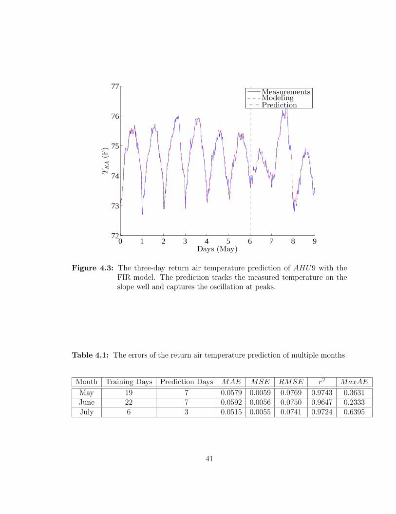
0 1 2 3 4 5 6 7 8 972

73

74

75

76

77

Days (May)

TRA(F

)

MeasurementsModelingPrediction

Figure 4.3: The three-day return air temperature prediction of AHU9 with theFIR model. The prediction tracks the measured temperature on theslope well and captures the oscillation at peaks.

Table 4.1: The errors of the return air temperature prediction of multiple months.

Month Training Days Prediction Days MAE MSE RMSE r2 MaxAE

May 19 7 0.0579 0.0059 0.0769 0.9743 0.3631June 22 7 0.0592 0.0056 0.0750 0.9647 0.2333July 6 3 0.0515 0.0055 0.0741 0.9724 0.6395

41

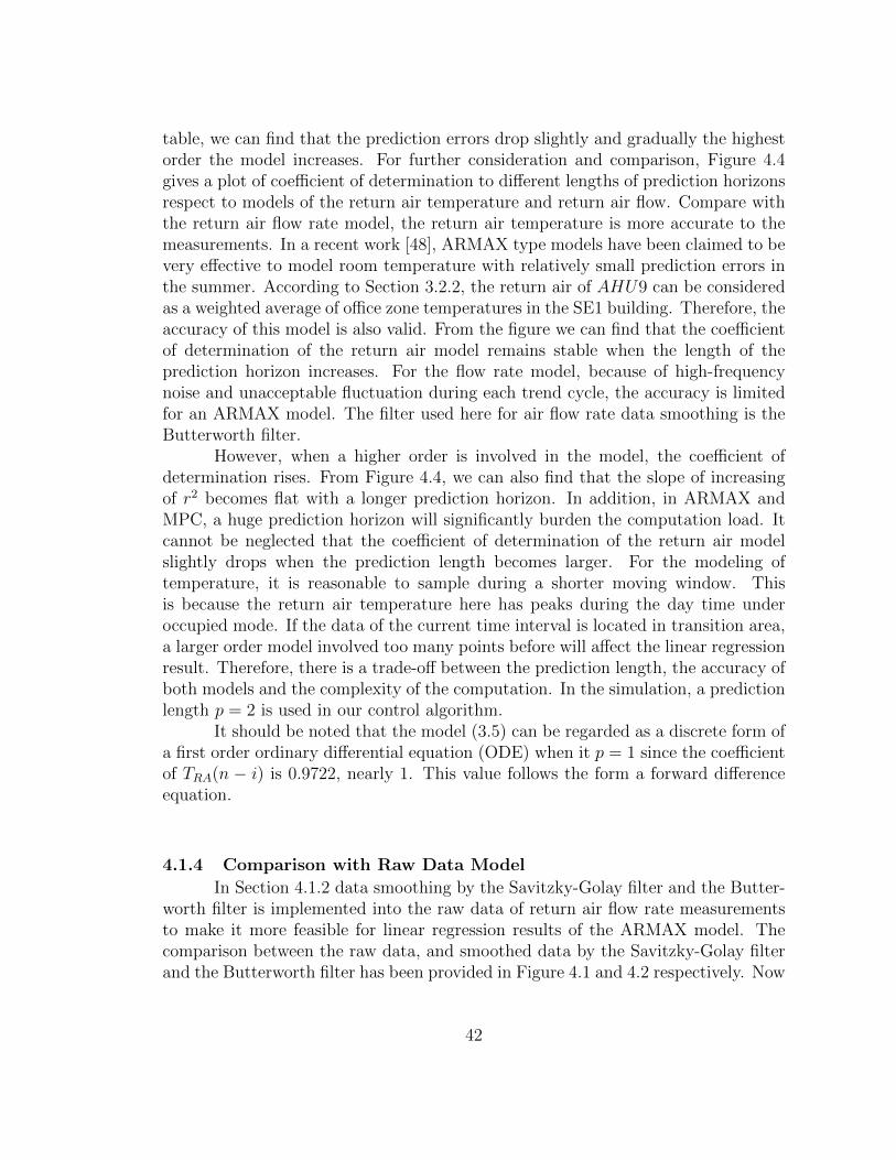
table, we can find that the prediction errors drop slightly and gradually the highestorder the model increases. For further consideration and comparison, Figure 4.4gives a plot of coefficient of determination to different lengths of prediction horizonsrespect to models of the return air temperature and return air flow. Compare withthe return air flow rate model, the return air temperature is more accurate to themeasurements. In a recent work [48], ARMAX type models have been claimed to bevery effective to model room temperature with relatively small prediction errors inthe summer. According to Section 3.2.2, the return air of AHU9 can be consideredas a weighted average of office zone temperatures in the SE1 building. Therefore, theaccuracy of this model is also valid. From the figure we can find that the coefficientof determination of the return air model remains stable when the length of theprediction horizon increases. For the flow rate model, because of high-frequencynoise and unacceptable fluctuation during each trend cycle, the accuracy is limitedfor an ARMAX model. The filter used here for air flow rate data smoothing is theButterworth filter.

However, when a higher order is involved in the model, the coefficient ofdetermination rises. From Figure 4.4, we can also find that the slope of increasingof r2 becomes flat with a longer prediction horizon. In addition, in ARMAX andMPC, a huge prediction horizon will significantly burden the computation load. Itcannot be neglected that the coefficient of determination of the return air modelslightly drops when the prediction length becomes larger. For the modeling oftemperature, it is reasonable to sample during a shorter moving window. Thisis because the return air temperature here has peaks during the day time underoccupied mode. If the data of the current time interval is located in transition area,a larger order model involved too many points before will affect the linear regressionresult. Therefore, there is a trade-off between the prediction length, the accuracy ofboth models and the complexity of the computation. In the simulation, a predictionlength p = 2 is used in our control algorithm.

It should be noted that the model (3.5) can be regarded as a discrete form ofa first order ordinary differential equation (ODE) when it p = 1 since the coefficientof TRA(n − i) is 0.9722, nearly 1. This value follows the form a forward differenceequation.

4.1.4 Comparison with Raw Data Model

In Section 4.1.2 data smoothing by the Savitzky-Golay filter and the Butter-worth filter is implemented into the raw data of return air flow rate measurementsto make it more feasible for linear regression results of the ARMAX model. Thecomparison between the raw data, and smoothed data by the Savitzky-Golay filterand the Butterworth filter has been provided in Figure 4.1 and 4.2 respectively. Now

42

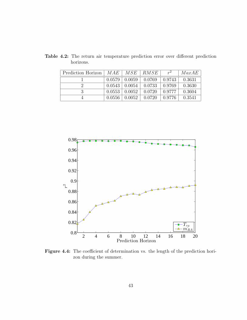
Table 4.2: The return air temperature prediction error over different predictionhorizons.

Prediction Horizon MAE MSE RMSE r2 MaxAE

1 0.0579 0.0059 0.0769 0.9743 0.36312 0.0543 0.0054 0.0733 0.9769 0.36303 0.0553 0.0052 0.0720 0.9777 0.36044 0.0556 0.0052 0.0720 0.9776 0.3541

2 4 6 8 10 12 14 16 18 200.8

0.82

0.84

0.86

0.88

0.9

0.92

0.94

0.96

0.98

Prediction Horizon

r2

Tra

˙mRA

Figure 4.4: The coefficient of determination vs. the length of the prediction hori-zon during the summer.

43

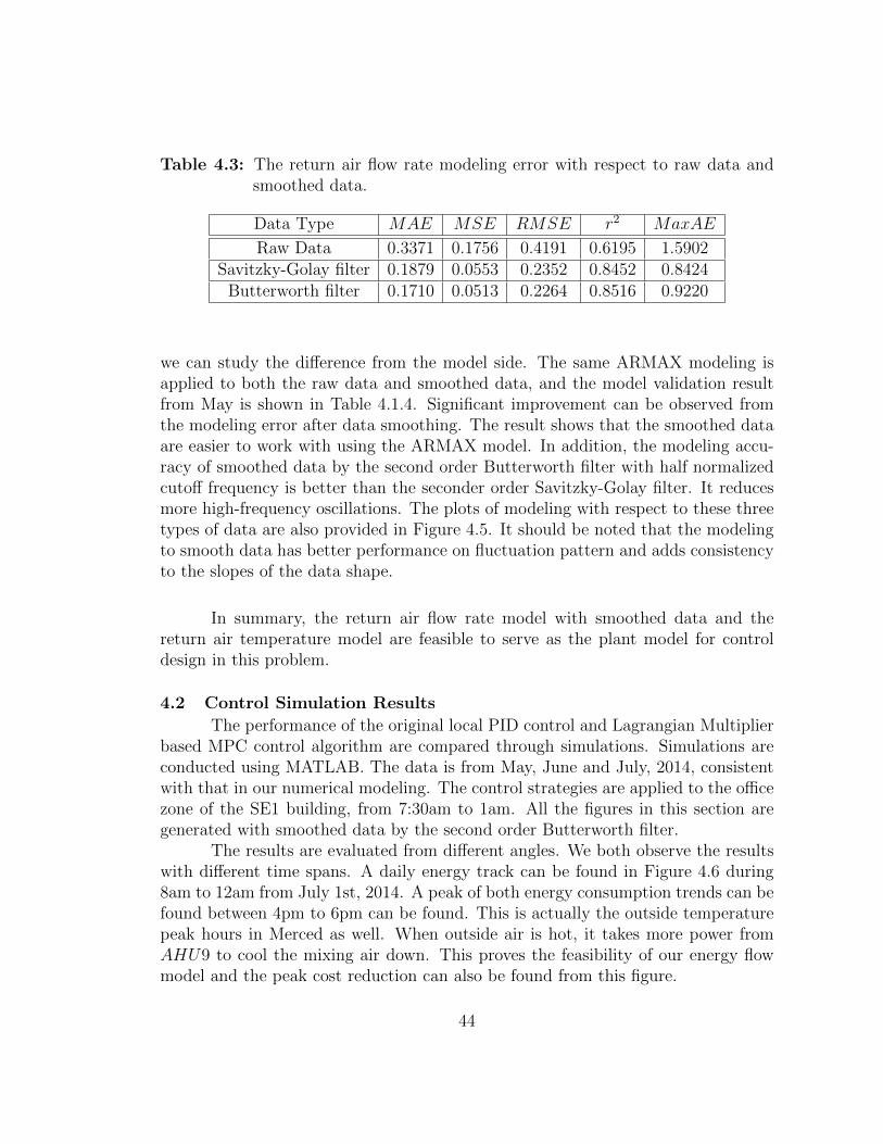
Table 4.3: The return air flow rate modeling error with respect to raw data andsmoothed data.

Data Type MAE MSE RMSE r2 MaxAE

Raw Data 0.3371 0.1756 0.4191 0.6195 1.5902Savitzky-Golay filter 0.1879 0.0553 0.2352 0.8452 0.8424

Butterworth filter 0.1710 0.0513 0.2264 0.8516 0.9220

we can study the difference from the model side. The same ARMAX modeling isapplied to both the raw data and smoothed data, and the model validation resultfrom May is shown in Table 4.1.4. Significant improvement can be observed fromthe modeling error after data smoothing. The result shows that the smoothed dataare easier to work with using the ARMAX model. In addition, the modeling accu-racy of smoothed data by the second order Butterworth filter with half normalizedcutoff frequency is better than the seconder order Savitzky-Golay filter. It reducesmore high-frequency oscillations. The plots of modeling with respect to these threetypes of data are also provided in Figure 4.5. It should be noted that the modelingto smooth data has better performance on fluctuation pattern and adds consistencyto the slopes of the data shape.

In summary, the return air flow rate model with smoothed data and thereturn air temperature model are feasible to serve as the plant model for controldesign in this problem.

4.2 Control Simulation Results

The performance of the original local PID control and Lagrangian Multiplierbased MPC control algorithm are compared through simulations. Simulations areconducted using MATLAB. The data is from May, June and July, 2014, consistentwith that in our numerical modeling. The control strategies are applied to the officezone of the SE1 building, from 7:30am to 1am. All the figures in this section aregenerated with smoothed data by the second order Butterworth filter.

The results are evaluated from different angles. We both observe the resultswith different time spans. A daily energy track can be found in Figure 4.6 during8am to 12am from July 1st, 2014. A peak of both energy consumption trends can befound between 4pm to 6pm can be found. This is actually the outside temperaturepeak hours in Merced as well. When outside air is hot, it takes more power fromAHU9 to cool the mixing air down. This proves the feasibility of our energy flowmodel and the peak cost reduction can also be found from this figure.

44

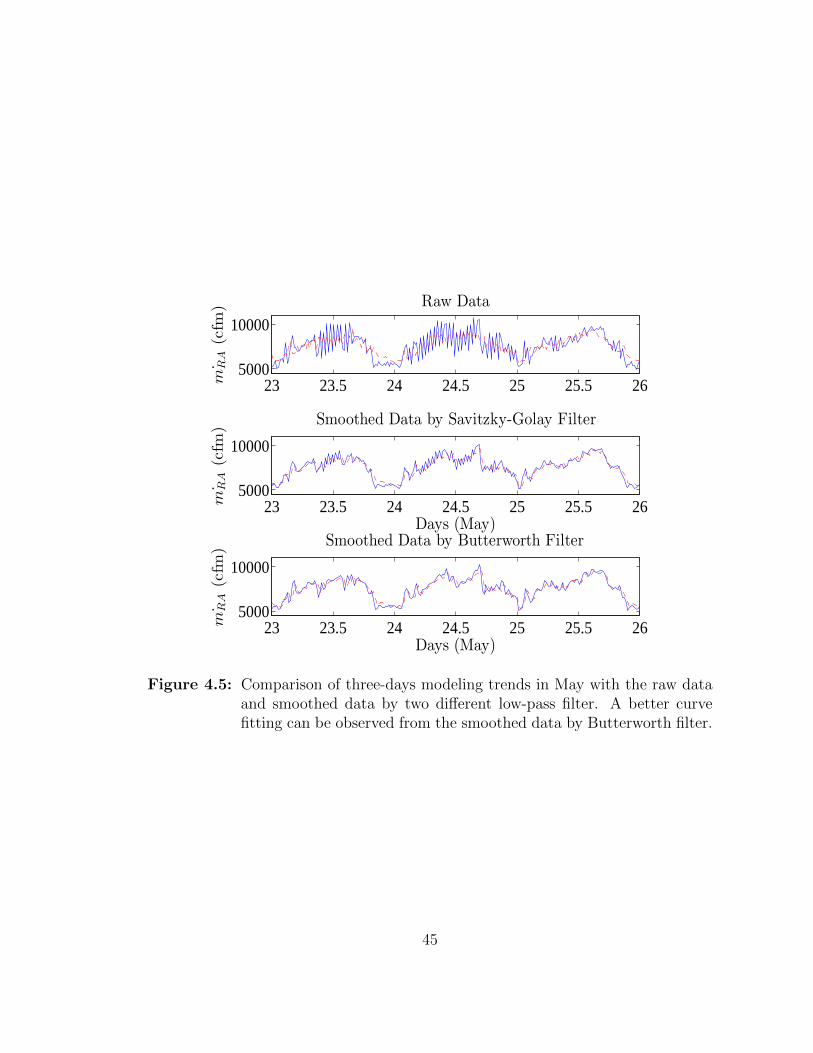
23 23.5 24 24.5 25 25.5 265000

10000

˙m

RA(cfm

) Raw Data

23 23.5 24 24.5 25 25.5 265000

10000

Days (May)

˙m

RA(cfm

)

Smoothed Data by Savitzky-Golay Filter

23 23.5 24 24.5 25 25.5 265000

10000

Days (May)

˙m

RA(cfm

)

Smoothed Data by Butterworth Filter

Figure 4.5: Comparison of three-days modeling trends in May with the raw dataand smoothed data by two different low-pass filter. A better curvefitting can be observed from the smoothed data by Butterworth filter.

45

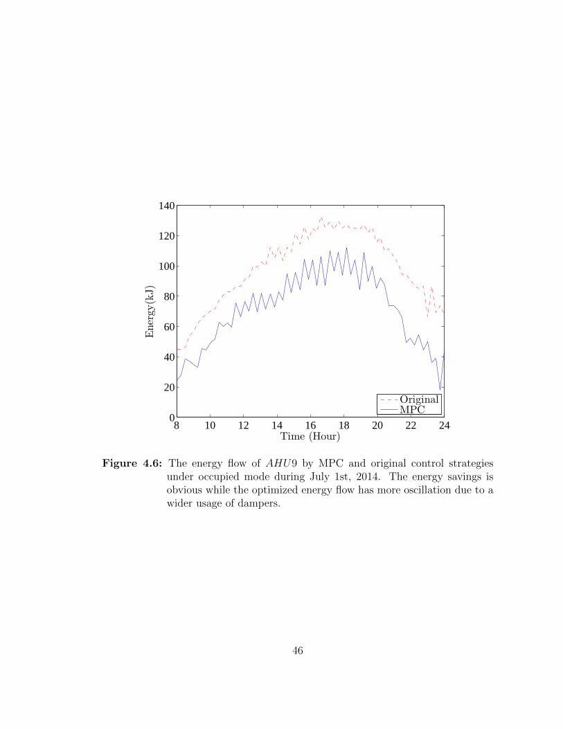
8 10 12 14 16 18 20 22 240

20

40

60

80

100

120

140

Time (Hour)

Energy

(kJ)

OriginalMPC

Figure 4.6: The energy flow of AHU9 by MPC and original control strategiesunder occupied mode during July 1st, 2014. The energy savings isobvious while the optimized energy flow has more oscillation due to awider usage of dampers.

46

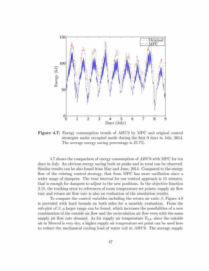
0 1 2 3 4 5 6 7 8 90

50

100

150

Days (July)

Energy

(kJ)

OriginalMPC

Figure 4.7: Energy consumption trends of AHU9 by MPC and original controlstrategies under occupied mode during the first 9 days in July, 2014.The average energy saving percentage is 25.7%.

4.7 shows the comparison of energy consumption of AHU9 with MPC for tendays in July. An obvious energy saving both at peaks and in total can be observed.Similar results can be also found from May and June, 2014. Compared to the energyflow of the existing control strategy, that from MPC has more oscillation since awider usage of dampers. The time interval for our control approach is 15 minutes,that is enough for dampers to adjust to the new positions. In the objective function3.15, the tracking error to references of room temperature set points, supply air flowrate and return air flow rate is also an evaluation of the simulation results.

To compare the control variables including the return air ratio β, Figure 4.8is provided with hard bounds on both sides for a monthly evaluation. From thesub-plot of β, a larger range can be found, which increases the possibilities of a newcombination of the outside air flow and the recirculation air flow even with the samesupply air flow rate demand. As for supply air temperature TSA, since the outsideair in Merced is very dry, a higher supply air temperature set point can be used hereto reduce the mechanical cooling load of water coil in AHU9. The average supply

47

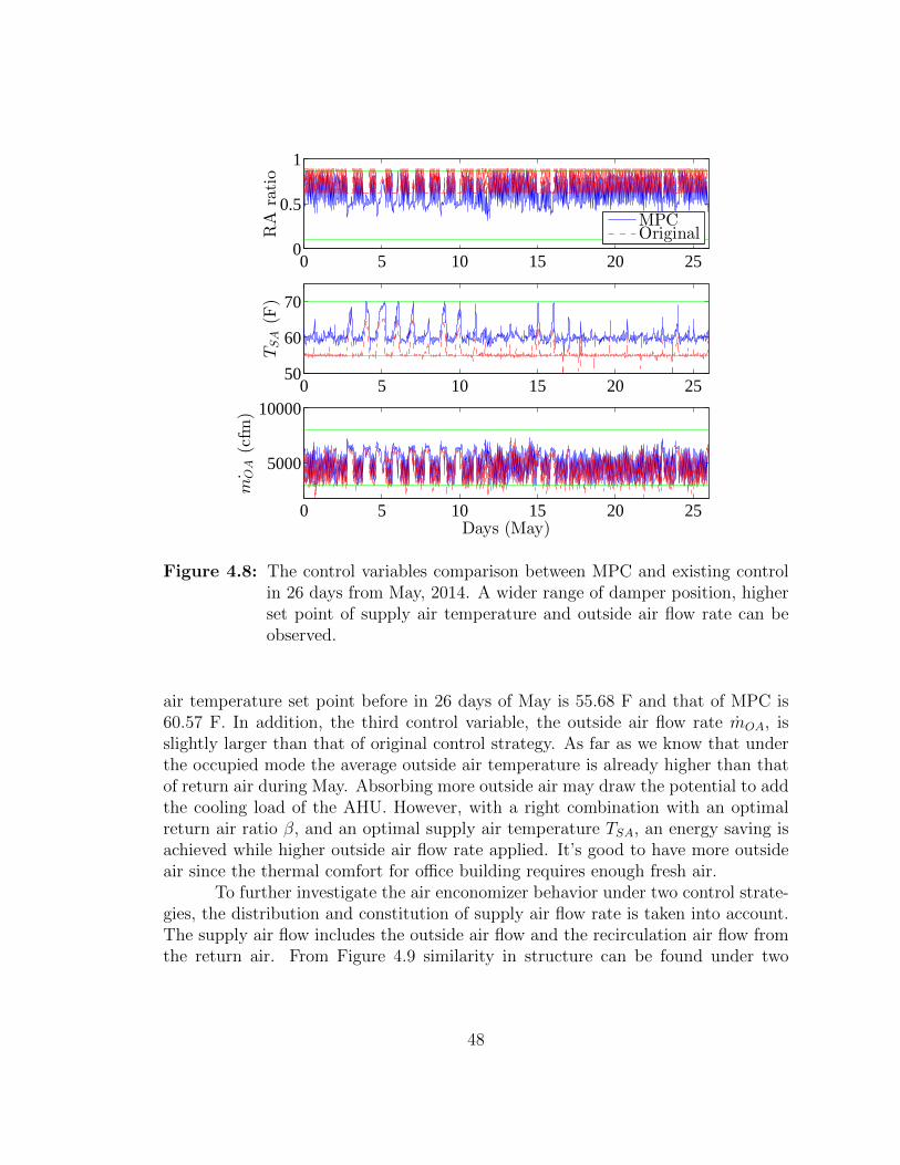
0 5 10 15 20 250

0.5

1

RA

ratio

MPCOriginal

0 5 10 15 20 2550

60

70

TSA(F

)

0 5 10 15 20 25

5000

10000

Days (May)

˙m

OA(cfm

)

Figure 4.8: The control variables comparison between MPC and existing controlin 26 days from May, 2014. A wider range of damper position, higherset point of supply air temperature and outside air flow rate can beobserved.

air temperature set point before in 26 days of May is 55.68 F and that of MPC is60.57 F. In addition, the third control variable, the outside air flow rate mOA, isslightly larger than that of original control strategy. As far as we know that underthe occupied mode the average outside air temperature is already higher than thatof return air during May. Absorbing more outside air may draw the potential to addthe cooling load of the AHU. However, with a right combination with an optimalreturn air ratio β, and an optimal supply air temperature TSA, an energy saving isachieved while higher outside air flow rate applied. It’s good to have more outsideair since the thermal comfort for office building requires enough fresh air.

To further investigate the air enconomizer behavior under two control strate-gies, the distribution and constitution of supply air flow rate is taken into account.The supply air flow includes the outside air flow and the recirculation air flow fromthe return air. From Figure 4.9 similarity in structure can be found under two

48

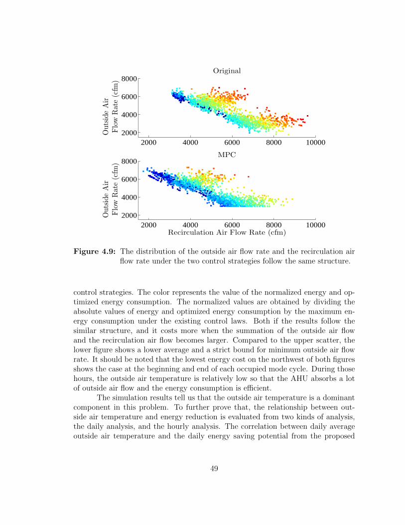
2000 4000 6000 8000 100002000

4000

6000

8000MPC

OutsideAir

Flow

Rate(cfm

)

Recirculation Air Flow Rate (cfm)

2000 4000 6000 8000 100002000

4000

6000

8000Original

OutsideAir

Flow

Rate(cfm

)

Figure 4.9: The distribution of the outside air flow rate and the recirculation airflow rate under the two control strategies follow the same structure.

control strategies. The color represents the value of the normalized energy and op-timized energy consumption. The normalized values are obtained by dividing theabsolute values of energy and optimized energy consumption by the maximum en-ergy consumption under the existing control laws. Both if the results follow thesimilar structure, and it costs more when the summation of the outside air flowand the recirculation air flow becomes larger. Compared to the upper scatter, thelower figure shows a lower average and a strict bound for minimum outside air flowrate. It should be noted that the lowest energy cost on the northwest of both figuresshows the case at the beginning and end of each occupied mode cycle. During thosehours, the outside air temperature is relatively low so that the AHU absorbs a lotof outside air flow and the energy consumption is efficient.

The simulation results tell us that the outside air temperature is a dominantcomponent in this problem. To further prove that, the relationship between out-side air temperature and energy reduction is evaluated from two kinds of analysis,the daily analysis, and the hourly analysis. The correlation between daily averageoutside air temperature and the daily energy saving potential from the proposed

49

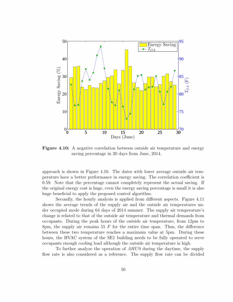
0 5 10 15 20 25 300

10

20

30

40

50

Days (June)

EnergySav

ing(%

)

0 5 10 15 20 25 3070

75

80

85

90

95

TOA(F

)

Energy SavingTOA

Figure 4.10: A negative correlation between outside air temperature and energysaving percentage in 20 days from June, 2014.

approach is shown in Figure 4.10. The dates with lower average outside air tem-perature have a better performance in energy saving. The correlation coefficient is0.59. Note that the percentage cannot completely represent the actual saving. Ifthe original energy cost is huge, even the energy saving percentage is small it is alsohuge beneficial to apply the proposed control algorithm.

Secondly, the hourly analysis is applied from different aspects. Figure 4.11shows the average trends of the supply air and the outside air temperatures un-der occupied mode during 64 days of 2014 summer. The supply air temperature’schange is related to that of the outside air temperature and thermal demands fromoccupants. During the peak hours of the outside air temperature, from 12pm to8pm, the supply air remains 55 F for the entire time span. Thus, the differencebetween these two temperature reaches a maximum value at 5pm. During thesehours, the HVAC system of the SE1 building needs to be fully operated to serveoccupants enough cooling load although the outside air temperature is high.

To further analyze the operation of AHU9 during the daytime, the supplyflow rate is also considered as a reference. The supply flow rate can be divided

50

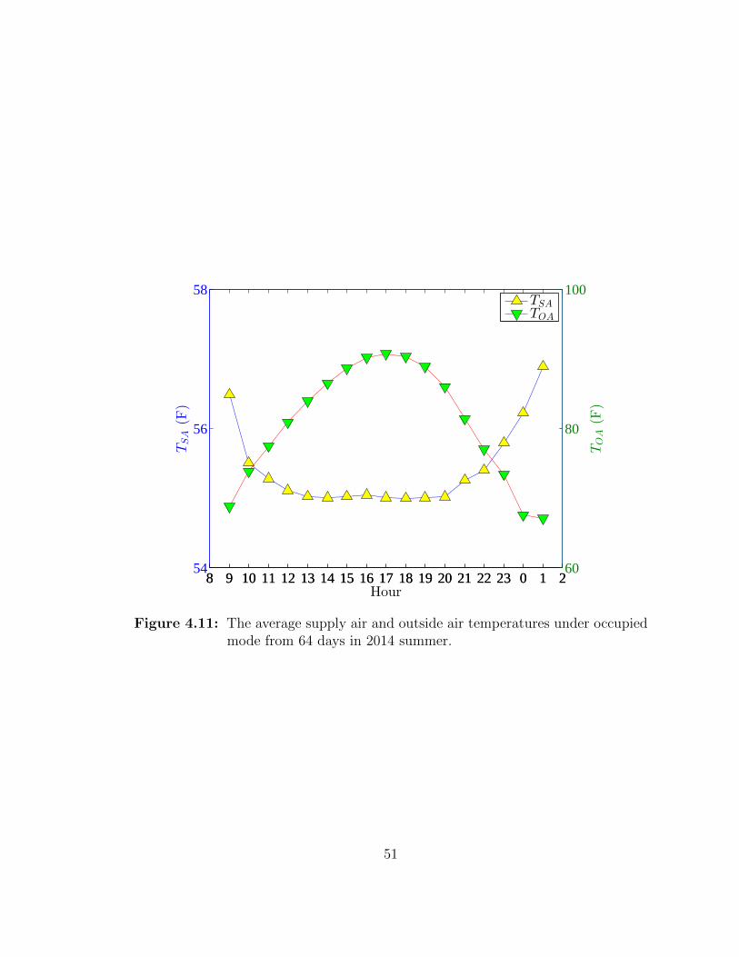
8 9 10 11 12 13 14 15 16 17 18 19 20 21 22 23 0 1 254

56

58

TSA(F

)

Hour8 9 10 11 12 13 14 15 16 17 18 19 20 21 22 23 0 1 2

60

80

100

TOA(F

)

TSA

TOA

Figure 4.11: The average supply air and outside air temperatures under occupiedmode from 64 days in 2014 summer.

51

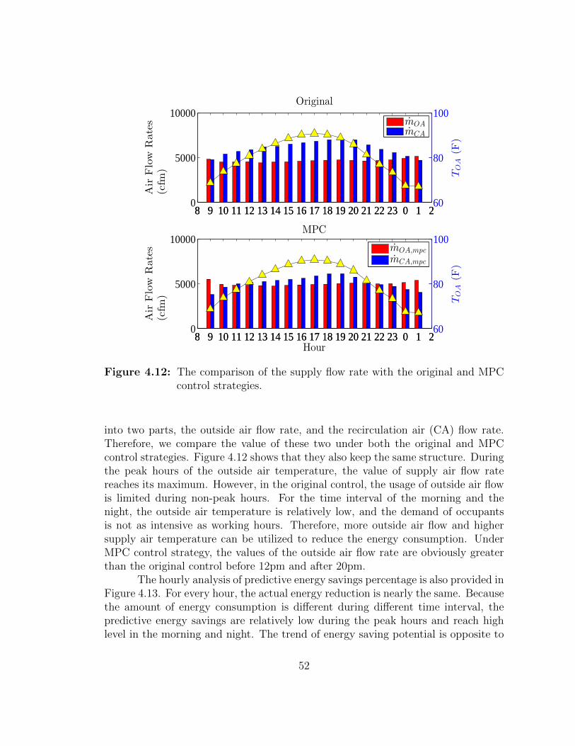
8 9 10 11 12 13 14 15 16 17 18 19 20 21 22 23 0 1 20

5000

10000

AirFlow

Rates

(cfm

)

Original

8 9 10 11 12 13 14 15 16 17 18 19 20 21 22 23 0 1 260

80

100

TOA(F

)

mOAmCA

8 9 10 11 12 13 14 15 16 17 18 19 20 21 22 23 0 1 20

5000

10000

Hour

AirFlow

Rates

(cfm

)

MPC

8 9 10 11 12 13 14 15 16 17 18 19 20 21 22 23 0 1 260

80

100

TOA(F

)

mOA,mpc

mCA,mpc

Figure 4.12: The comparison of the supply flow rate with the original and MPCcontrol strategies.

into two parts, the outside air flow rate, and the recirculation air (CA) flow rate.Therefore, we compare the value of these two under both the original and MPCcontrol strategies. Figure 4.12 shows that they also keep the same structure. Duringthe peak hours of the outside air temperature, the value of supply air flow ratereaches its maximum. However, in the original control, the usage of outside air flowis limited during non-peak hours. For the time interval of the morning and thenight, the outside air temperature is relatively low, and the demand of occupantsis not as intensive as working hours. Therefore, more outside air flow and highersupply air temperature can be utilized to reduce the energy consumption. UnderMPC control strategy, the values of the outside air flow rate are obviously greaterthan the original control before 12pm and after 20pm.

The hourly analysis of predictive energy savings percentage is also provided inFigure 4.13. For every hour, the actual energy reduction is nearly the same. Becausethe amount of energy consumption is different during different time interval, thepredictive energy savings are relatively low during the peak hours and reach highlevel in the morning and night. The trend of energy saving potential is opposite to

52

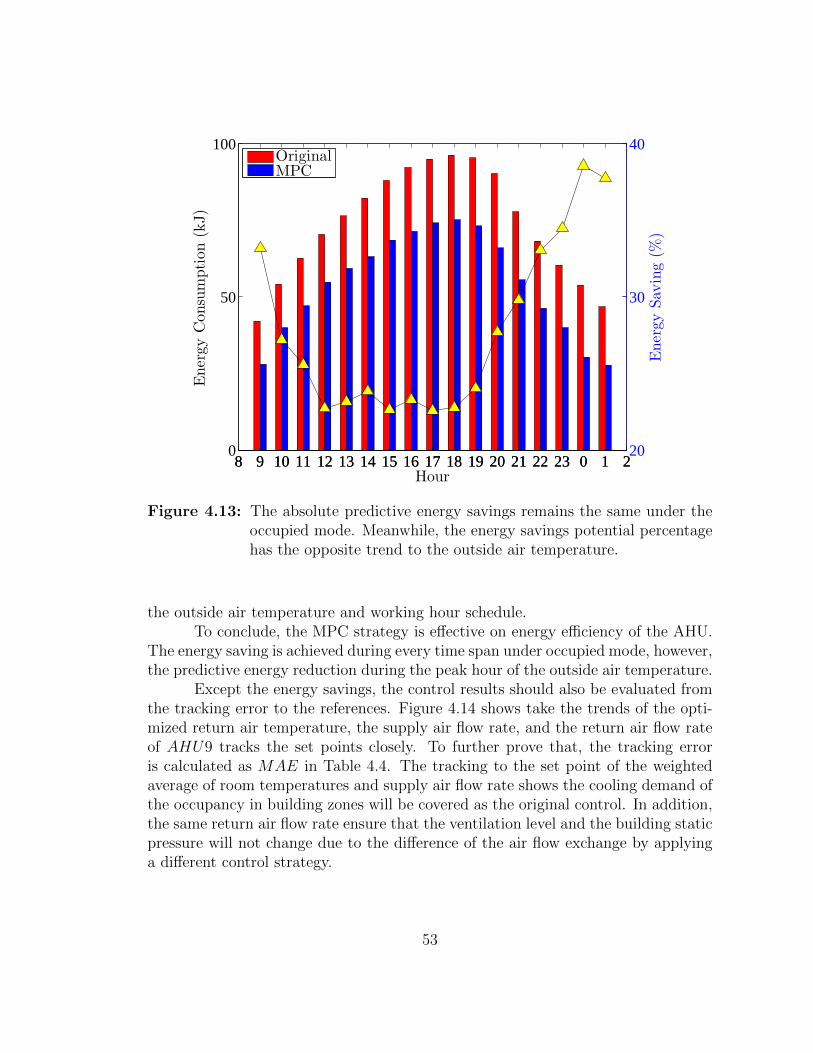
8 9 10 11 12 13 14 15 16 17 18 19 20 21 22 23 0 1 20

50

100

Hour

EnergyConsumption(kJ)

8 9 10 11 12 13 14 15 16 17 18 19 20 21 22 23 0 1 220

30

40

EnergySav

ing(%

)

OriginalMPC

Figure 4.13: The absolute predictive energy savings remains the same under theoccupied mode. Meanwhile, the energy savings potential percentagehas the opposite trend to the outside air temperature.

the outside air temperature and working hour schedule.To conclude, the MPC strategy is effective on energy efficiency of the AHU.

The energy saving is achieved during every time span under occupied mode, however,the predictive energy reduction during the peak hour of the outside air temperature.

Except the energy savings, the control results should also be evaluated fromthe tracking error to the references. Figure 4.14 shows take the trends of the opti-mized return air temperature, the supply air flow rate, and the return air flow rateof AHU9 tracks the set points closely. To further prove that, the tracking erroris calculated as MAE in Table 4.4. The tracking to the set point of the weightedaverage of room temperatures and supply air flow rate shows the cooling demand ofthe occupancy in building zones will be covered as the original control. In addition,the same return air flow rate ensure that the ventilation level and the building staticpressure will not change due to the difference of the air flow exchange by applyinga different control strategy.

53

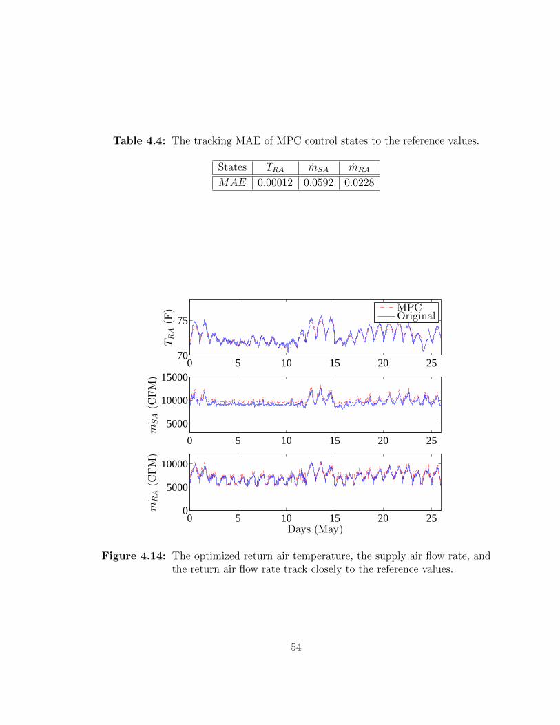
Table 4.4: The tracking MAE of MPC control states to the reference values.

States TRA mSA mRA

MAE 0.00012 0.0592 0.0228

0 5 10 15 20 2570

75

TRA(F

) MPCOriginal

0 5 10 15 20 25

5000

10000

15000

˙m

SA(C

FM)

0 5 10 15 20 250

5000

10000

Days (May)

˙m

RA(C

FM)

Figure 4.14: The optimized return air temperature, the supply air flow rate, andthe return air flow rate track closely to the reference values.

54

Chapter 5

SUMMARY AND FUTURE WORK

5.1 Concluding Remarks

To leverage the untapped capabilities of modern building automation andcontrol systems, we have developed a system-level dynamical model and MPC con-trol design of HVAC systems. Works in this thesis focus on two functionalities, i.e.,modeling and control. As for modeling, we have used a return air dynamical modelto link the current temperature and flow rate states of the building and the controlvariables, that is accurate for prediction and friendly to control implementation.With regard to control, based on the model we built serving as a plant, a MPCalgorithm is applied to the HVAC energy management system. This MPC strategyutilizes different levels of HVAC units in buildings. The control results show a signif-icant energy saving meanwhile keep the same level of building cooling load, thermalcomfort and static pressure. This algorithm can be applied on system-wide scalesto optimize overall system performance and help achieve the goal of zero energyconsumption.

5.1.1 Model

We have developed a FIR-based return air model from the AHU return airdynamics for both temperature and air flow rate. The proposed model has predictionand control horizon flexibility and much few variables compared to a fully numericalmodel. Trained with the data over a short and long time frame, the proposedmodel is capable of predicting the return air temperature with a high accuracy. Forexample, the AHU return air temperature model trained with the data from 2014summer can predict the return air temperature over one week with mean squarederrors less than 0.006 and coefficients of determination above 0.97 on average. Wehave also shown the relationship between prediction steps and the accuracy of themodel. An optimal prediction horizon provides a trade-off between model accuracyand computation load. With the right choice of prediction horizon, the dynamicalmodel further improves its prediction performance, and could be a basis for MPCcontrol design of HVAC systems.

Otherwise, we implement Savitzky-Golay filter during data pre-processing fordata smoothing. Measurements of air flow rate inside HVAC systems is vulnerable

55

to sensor noise and resistant to model parameter identification. Savitzky-Golay filtertakes a moving average of the measurements and serves as a low-pass filter. Aftersmoothing, the curve fitting performance becomes better and could be used as aplant of an MPC controller of HVAC systems.

It should be noted that this model could also be used to predict other pa-rameters of interest in HVAC simulations, e.g., the relative humidity and parts permillion (ppm) of CO2. We are trying to corporate this model with the relativehumidity sensors and CO2 sensors of other latest buildings on UC Merced campus.

5.1.2 Control

We have established a system-level MPC control strategy for building HVACsystems. Energy description of the AHU and the gradient-based optimization andthe cross-level constraints and objectives are three key elements of the method. Theenergy flow model provides the possibilities of variable distribution of outside airand recirculation air. This energy feature helps energy saving of the HVAC sys-tem and cover the thermal demand of the building, as well as preserve the samestatic pressure and ventilation level. The control strategy uses damper positions,supply air temperature and outside air flow rate as control variables. They areexplicitly implemented into both the models and objective functions. The strate-gy provides physical-based inherent connection between components in AHU, andconsiders cross-level constraints in the whole HVAC system of SE1 building. Forthe optimization procedure, the gradient follows a fine structure due to the typesof objective functions and the involvement of Lagrangian Multiplier. It might bean indefinite symmetric matrix, thus this linear system can be solved efficiently bysome factorization method such. The optimal results show an energy saving aver-age percentage over 27.8% and track the supply air flow rate and set point of roomtemperatures in the building pretty well. The thermal load, supply air flow rateset points are calculated from thirty-two VAVs, that ensures the internal coolingdemand, the static pressure, and the ventilation level of the building.

This control strategy is implemented into the WebCTRL R©of the SE1 build-ing and can be easily incorporated with other BAS as well since the explicit formu-lation.

5.2 Future Work

5.2.1 MPC of HVAC systems with Humidity and CO2 Control

Due to the scarcity of humidity sensors in SE1 building, the humidity controlcannot be considered in our approach. However, the climate in Merced secures thepossibilities to change supply air temperature without sacrificing the thermal com-fort from humidity side. We shall implement this MPC algorithm with LagrangianMultiplier into other environment conditions, like San Francisco and Miami. Also,if we want to apply this approach to other types of commercial building, such as

56

gyms, lounges, and data centers. the indoor humidity and frequency of air flowdischarging will definitely need to change. Therefore, the enthalpy and humiditybalance need to be involved in the air flow dynamical models and energy balancemodel.

The newly built buildings on UC Merced campus, Social Science and Manage-ment (SSM) Building, Student Service Building (SSB) and Science and EngineeringBuilding II (SE2) are equipped with intelligent humidity sensors. It should be notedthat CO2 sensors are also available in the HVAC systems of these buildings. Theppm of CO2 can be an effective index of both ventilation and thermal comfort e-valuation. Similar patterns can be followed to also implement CO2 control to theproposed method as that of humidity.

5.2.2 Online Implementation of MPC to Building HVAC Systems

We shall expand and enhance the gradient-based MPC algorithm by applyingfuzzy control laws. We need to restore historic data and group them by seasonal,monthly, weekly, daily, and hourly time partition. The existing control strategies,the internal thermal load, and climate can be saved as references to the MPC al-gorithm. If the predicted energy consumption and thermal comfort level is not asgood as the existing control laws under similar model states, we shall stick to theoriginal control variable before.

We shall also complete the real-time building HVAC system commissioningwith the proposed control strategy. Figure 5.1 shows the workflow of an online MPCof building HVAC systems. Specifically, the online receding algorithm can be dividedinto several steps. First, an automatic data acquisition and pre-processing module isneeded. For an online user interface BAS, such as WebCTRL R©, data from originalsensor measurements can be collected over the web service by adopting structuredinformation exchanging implementation, such as the Simple Object Access Protocol(SOAP). Digital filters, like Savitzky-Golay filter we used in Chapter 4, will be alsodesigned to reduce the measurement noise. Next, data-driven models can be builtfrom the stored data, as well as all the past operational records, internal thermalload of the office zone and climate conditions at that time. Then we apply theMPC algorithm to the real-time data by choosing right model and compute thefuture control input. After that, a evaluation of objective functions, like energysaving and thermal comfort will be calculated between the existing mode and theoptimal control. A decision will be made to take or not take the computed controlvariables. At last, the control result will be recorded and the model will be updatedand imposed on new data in the time domain.

We shall also develop a graphical user interface (GUI) to present the MPCobjective functions and constraints in a user-friendly and informative manner. Thus,the result can be shown up. According to the real-time data trend, the MPC results

57

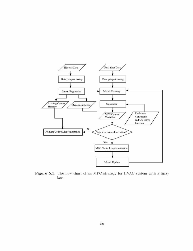
Figure 5.1: The flow chart of an MPC strategy for HVAC system with a fuzzylaw.

58

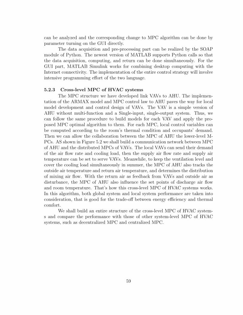
can be analyzed and the corresponding change to MPC algorithm can be done byparameter turning on the GUI directly.

The data acquisition and pre-processing part can be realized by the SOAPmodule of Python. The newest version of MATLAB supports Python calls so thatthe data acquisition, computing, and return can be done simultaneously. For theGUI part, MATLAB Simulink works for combining desktop computing with theInternet connectivity. The implementation of the entire control strategy will involveintensive programming effort of the two language.

5.2.3 Cross-level MPC of HVAC systems

The MPC structure we have developed link VAVs to AHU. The implemen-tation of the ARMAX model and MPC control law to AHU paves the way for localmodel development and control design of VAVs. The VAV is a simple version ofAHU without multi-function and a Single-input, single-output system. Thus, wecan follow the same procedure to build models for each VAV and apply the pro-posed MPC optimal algorithm to them. For each MPC, local control variables canbe computed according to the room’s thermal condition and occupants’ demand.Then we can allow the collaboration between the MPC of AHU the lower-level M-PCs. AS shown in Figure 5.2 we shall build a communication network between MPCof AHU and the distributed MPCs of VAVs. The local VAVs can send their demandof the air flow rate and cooling load, then the supply air flow rate and supply airtemperature can be set to serve VAVs. Meanwhile, to keep the ventilation level andcover the cooling load simultaneously in summer, the MPC of AHU also tracks theoutside air temperature and return air temperature, and determines the distributionof mixing air flow. With the return air as feedback from VAVs and outside air asdisturbance, the MPC of AHU also influence the set points of discharge air flowand room temperature. That’s how this cross-level MPC of HVAC systems works.In this algorithm, both global system and local system performance are taken intoconsideration, that is good for the trade-off between energy efficiency and thermalcomfort.

We shall build an entire structure of the cross-level MPC of HVAC system-s and compare the performance with those of other system-level MPC of HVACsystems, such as decentralized MPC and centralized MPC.

59

Figure 5.2: A future structure of cross-level MPC framework with a communica-tion network.

60

BIBLIOGRAPHY

[1] http://www.cacx.org/meetings/meetings/2012-08-09/NBI CCC Webinar 080912.pdf, Fault detection & diagnostics (FDD)rooftop HVAC units: Technology, code requirements, commissioning.

[2] http://buildingsdatabook.eren.doe.gov/TableView.aspx?table=1.1.1, U.S.residential and commercial buildings total primary energy consumption(quadrillion btu and percent of total) (2011).

[3] http://buildingsdatabook.eren.doe.gov/TableView.aspx?table=1.1.3, Build-ings share of U.S. primary energy consumption (percent) (2011).

[4] http://buildingsdatabook.eren.doe.gov/TableView.aspx?table=1.1.9, Build-ings share of U.S. electricity consumption (percent) (2011).

[5] U. EIA, Annual energy outlook 2014, Tech. rep. (2014).

[6] A. S. ASHRAE, Standard 90.1-2004, Energy standard for buildings exceptlow rise residential buildings, American Society of Heating, Refrigerating andAir-Conditioning Engineers, Inc.

[7] C. E. Commission, 2013 Building Energy Efficiency Standards for Residentialand Nonresidential Buildings, California Energy Commission, 2013.

[8] K. I. Krakow, S. Lin, PI control of fan speed to maintain constant dischargepressure, ASHRAE Transactions-American Society of Heating RefrigeratingAirconditioning Engin 101 (2) (1995) 398–407.

[9] I. Jette, M. Zaheer-Uddin, P. Fazio, PI-control of dual duct systems: man-ual tuning and control loop interaction, Energy conversion and management39 (14) (1998) 1471–1482.

[10] J. Bai, S. Wang, X. Zhang, Development of an adaptive smith predictor-basedself-tuning PI controller for an HVAC system in a test room, Energy andBuildings 40 (12) (2008) 2244–2252.

[11] Q. Bi, W.-J. Cai, Q.-G. Wang, C.-C. Hang, E.-L. Lee, Y. Sun, K.-D. Liu,Y. Zhang, B. Zou, Advanced controller auto-tuning and its application inHVAC systems, Control Engineering Practice 8 (6) (2000) 633–644.

61

[12] T. Salsbury, A survey of control technologies in the building automation in-dustry, in: the 16th IFAC World Congress, 2005, pp. 1396–1407.

[13] D. S. Naidu, C. G. Rieger, Advanced control strategies for heating, ventilation,air-conditioning, and refrigeration systemsAn overview: Part I: Hard control,HVACR Research 17 (1) (2011) 2–21.

[14] X.-D. He, H. H. Asada, A new feedback linearization approach to advancedcontrol of multi-unit HVAC systems, in: American Control Conference, 2003.Proceedings of the 2003, Vol. 3, IEEE, 2003, pp. 2311–2316.

[15] H. Moradi, M. Saffar-Avval, F. Bakhtiari-Nejad, Nonlinear multivariable con-trol and performance analysis of an air-handling unit, Energy and Buildings43 (4) (2011) 805–813.

[16] S. Wang, X. Xu, Optimal and robust control of outdoor ventilation airflow ratefor improving energy efficiency and IAQ, Building and Environment 39 (7)(2004) 763–773.

[17] J. House, T. Smith, J. Arora, Optimal control of a thermal system, ASHRAETransactions 97 (2) (1991) 991–1001.

[18] S. Wang, X. Jin, Model-based optimal control of VAV air-conditioning systemusing genetic algorithm, Building and Environment 35 (6) (2000) 471–487.

[19] A. Kusiak, G. Xu, Modeling and optimization of HVAC systems using a dy-namic neural network, Energy 42 (1) (2012) 241–250.

[20] A. I. Dounis, C. Caraiscos, Advanced control systems engineering for energyand comfort management in a building environment-A review, Renewable andSustainable Energy Reviews 13 (6) (2009) 1246–1261.

[21] S. A. Kalogirou, Artificial neural networks and genetic algorithms in energyapplications in buildings, Advances in Building Energy Research 3 (1) (2009)83–119.

[22] S. A. Klein, TRNSYS, a transient system simulation program, Solar EnergyLaborataory, University of Wisconsin–Madison, 1979.

[23] L. Magnier, F. Haghighat, Multiobjective optimization of building design us-ing TRNSYS simulations, genetic algorithm, and Artificial Neural Network,Building and Environment 45 (3) (2010) 739–746.

[24] J. Liang, R. Du, Thermal comfort control based on neural network for HVACapplication, in: Control Applications, IEEE, 2005, pp. 819–824.

62

[25] D. Kolokotsa, D. Tsiavos, G. Stavrakakis, K. Kalaitzakis, E. Antonidakis, Ad-vanced fuzzy logic controllers design and evaluation for buildings occupantsthermalvisual comfort and indoor air quality satisfaction, Energy and build-ings 33 (6) (2001) 531–543.

[26] S. Prıvara, J. Cigler, Z. Vana, F. Oldewurtel, C. Sagerschnig, E. Zacekova,Building modeling as a crucial part for building predictive control, Energy andBuildings 56 (2013) 8–22.

[27] D. S. Naidu, C. G. Rieger, Advanced control strategies for heating, ventila-tion, air-conditioning, and refrigeration systemsAn overview: Part II: Soft andfusion control, HVACR Research 17 (2) (2011) 144–158.

[28] A. Afram, F. Janabi-Sharifi, Theory and applications of HVAC control sys-temsA review of model predictive control (MPC), Building and Environment72 (2014) 343–355.

[29] J. Siroky, F. Oldewurtel, J. Cigler, S. Prıvara, Experimental analysis of modelpredictive control for an energy efficient building heating system, AppliedEnergy 88 (9) (2011) 3079–3087.

[30] M. Maasoumy, A. Sangiovanni-Vincentelli, Total and peak energy consump-tion minimization of building HVAC systems using model predictive control,IEEE Design Test of Computers 29 (4).

[31] P.-D. Morosan, R. Bourdais, D. Dumur, J. Buisson, Building temperatureregulation using a distributed model predictive control, Energy and Buildings42 (9) (2010) 1445–1452.

[32] S. Prıvara, J. Siroky, L. Ferkl, J. Cigler, Model predictive control of a buildingheating system: The first experience, Energy and Buildings 43 (2) (2011) 564–572.

[33] A. Aswani, N. Master, J. Taneja, D. Culler, C. Tomlin, Reducing transientand steady state electricity consumption in hvac using learning-based model-predictive control, Proceedings of the IEEE 100 (1) (2012) 240–253.

[34] H. Lu, L. Jia, S. Kong, Z. Zhang, Predictive functional control based on fuzzyTS model for HVAC systems temperature control, Journal of Control Theoryand Applications 5 (1) (2007) 94–98.

[35] G. Huang, Model predictive control of VAV zone thermal systems concerningbi-linearity and gain nonlinearity, Control Engineering Practice 19 (7) (2011)700–710.

63

[36] M. Maasoumy, Comparison of control strategies for energy efficient buildingHVAC systems, in: ACM Symposium on Simulation for Architecture andUrban Design (SimAUD 2014), 2014.

[37] J. Rehrl, M. Horn, Temperature control for HVAC systems based on exactlinearization and model predictive control, in: Control Applications (CCA),IEEE, 2011, pp. 1119–1124.

[38] H. Yoshida, S. Kumar, RARX algorithm based model development and appli-cation to real time data for on-line fault detection in VAV AHU units, IBPSABuilding Simulation 99 (1999) 161–168.

[39] B. Tashtoush, M. Molhim, M. Al-Rousan, Dynamic model of an HVAC systemfor control analysis, Energy 30 (10) (2005) 1729–1745.

[40] P. O. Fanger, Thermal Comfort, Danish Technical Press., Copenhagen, 1970.

[41] P. O. Fanger, A. K. Melikov, H. Hanzawa, J. Ring, Air turbulence and sensa-tion of draught, Energy and Buildings 12 (1) (1988) 21–39.

[42] American Society of Heating Refrigerating and Air Conditioning Engineer-s (ASHARE), Thermal Environmental Conditions for Human Occupancy(ASHARE, Standard 55-1992).

[43] International Standards Organization (ISO), Moderate Thermal Environ-ments: Determination of the PMV and PPD Indices and Specification of theConditions for Thermal Comfort (ISO 7730:1994).

[44] S. Wang, X. Xu, Parameter estimation of internal thermal mass of buildingdynamic models using genetic algorithm, Energy Conversion and Management47 (13) (2006) 1927–1941.

[45] A. Thosar, A. Patra, S. Bhattacharyya, Feedback linearization based controlof a variable air volume air conditioning system for cooling applications, ISAtransactions 47 (3) (2008) 339–349.

[46] G. J. Rıos-Moreno, M. Trejo-Perea, R. Castaneda-Miranda, V. M. Hernandez-Guzman, G. Herrera-Ruiz, Modelling temperature in intelligent buildings bymeans of autoregressive models, Automation in Construction 16 (5) (2007)713–722.

[47] J. C. M. Yiu, S. Wang, Multiple ARMAX modeling scheme for forecasting airconditioning system performance, Energy Conversion and Management 48 (8)(2007) 2276–2285.

64

[48] G. Mustafaraj, J. Chen, G. Lowry, Development of room temperature andrelative humidity linear parametric models for an open office using BMS data,Energy and Buildings 42 (3) (2010) 348–356.

[49] X.-C. Xi, A.-N. Poo, S.-K. Chou, Support vector regression model predictivecontrol on a HVAC plant, Control Engineering Practice 15 (8) (2007) 897–908.

[50] S. Wu, J. Q. Sun, A physics-based linear parametric model of room tem-perature in office buildings, Building and Environment 50 (2012) 1–9, DOI:10.1016/j.buildenv.2011.10.005.

[51] S. Wu, J.-Q. Sun, Multi-stage regression linear parametric models of roomtemperature in office buildings, Building and Environment 56 (2012) 69–77.

[52] S. Wu, J. Q. Sun, Two-stage regression model of thermal comfort in officebuildings, Building and Environment 57 (2012) 88–96.

[53] S. Wu, System-level monitoring and diagnosis of building hvac system, Ph.D.thesis, University of California, Merced (2013).

[54] D. B. Crawley, L. K. Lawrie, C. O. Pedersen, F. C. Winkelmann, Energy plus:energy simulation program, ASHRAE journal 42 (4) (2000) 49–56.

[55] T. Chow, G. Zhang, Z. Lin, C. Song, Global optimization of absorption chillersystem by genetic algorithm and neural network, Energy and buildings 34 (1)(2002) 103–109.

[56] G.-Y. Jin, W.-J. Cai, L. Lu, E. L. Lee, A. Chiang, A simplified modelingof mechanical cooling tower for control and optimization of HVAC systems,Energy conversion and management 48 (2) (2007) 355–365.

[57] W. Wang, S. Katipamula, Y. Huang, M. R. Brambley, Energy savings andeconomics of advanced control strategies for packaged air conditioners withgas heat, Energy and Buildings 65 (2013) 497–507.

[58] Y.-W. Wang, W.-J. Cai, Y.-C. Soh, S.-J. Li, L. Lu, L. Xie, A simplified mod-eling of cooling coils for control and optimization of HVAC systems, EnergyConversion and Management 45 (18) (2004) 2915–2930.

[59] K. F. Fong, V. I. Hanby, T.-T. Chow, HVAC system optimization for ener-gy management by evolutionary programming, Energy and Buildings 38 (3)(2006) 220–231.

[60] J. E. Seem, Air handling unit including control system that prevents outsideair from entering the unit through an exhaust air damper (1998).

65

[61] G. Wang, M. Liu, Optimal outside air control for air handling units withhumidity control, in: Proceedings of the 6th International Conference for En-hanced Building Operations, Shenzhen, China, 2006.

[62] S. Yuan, R. A. Perez, Model predictive control of supply air temperatureand outside air intake rate of a VAV air-handling unit, ASHRAE transactions(2006) 145–161.

[63] N. Nassif, S. Moujaes, A new operating strategy for economizer dampers ofVAV system, Energy and Buildings 40 (3) (2008) 289–299.

[64] N. Nassif, Performance analysis of supply and return fans for HVAC systemsunder different operating strategies of economizer dampers, Energy and Build-ings 42 (7) (2010) 1026–1037.

[65] J. Seem, J. House, Development and evaluation of optimization-based air e-conomizer strategies, Applied Energy 87 (3) (2010) 910–924.

[66] G. Wang, L. Song, Air handling unit supply air temperature optimal controlduring economizer cycles, Energy and Buildings 49 (2012) 310–316.

[67] B. A. Ogunnaike, W. H. Ray, Process Dynamics, Modeling, and Control,Vol. 9, Oxford University Press New York, 1994.

[68] M. A. Henson, D. E. Seborg, Nonlinear Process Control, Prentice-Hall, Inc.,1997.

[69] E. F. Camacho, C. B. Alba, Model Predictive Control, Springer, 2013.

[70] J. V. Candy, Signal processing: model based approach, McGraw-Hill, Inc.,1986.

[71] D. P. Bertsekas, Nonlinear Programming, 1999.

[72] P. E. Gill, W. Murray, M. H. Wright, Practical Optimization, 1981.

[73] A. E. Bryson, Applied Optimal Control: Optimization, Estimation and Con-trol, CRC Press, 1975.

[74] K. Zhou, J. C. Doyle, K. Glover, Robust and Optimal Control, Vol. 40, Pren-tice Hall New Jersey, 1996.

[75] K. R. Muske, J. W. Howse, G. A. Hansen, Lagrangian solution methods fornonlinear model predictive control, in: American Control Conference, 2000.Proceedings of the 2000, Vol. 6, IEEE, 2000, pp. 4239–4243.

66

[76] P. TøNdel, T. A. Johansen, A. Bemporad, An algorithm for multi-parametricquadratic programming and explicit MPC solutions, Automatica 39 (3) (2003)489–497.

[77] M. Hovd, Multi-level programming for designing penalty functions for MPCcontrollers, in: Proceedings of the 18th IFAC World Congress, 2011, pp. 6098–6103.

[78] S. Richter, M. Morari, C. N. Jones, Towards computational complexity certifi-cation for constrained MPC based on lagrange relaxation and the fast gradientmethod, in: Decision and Control and European Control Conference (CDC-ECC), IEEE, 2011, pp. 5223–5229.

[79] V. Nedelcu, I. Necoara, Iteration complexity of an inexact augmented la-grangian method for constrained MPC, in: Decision and Control (CDC), 2012,pp. 650–655.

[80] G. Knabe, C. Felsmann, Optimal operation control of HVAC systems, in:Proceedings of 5th IBPSA Conference, 1997.

[81] L. Marletta, A comparison of methods for optimizing air-conditioning systemsaccording to the exergonomic approach, Journal of energy resources technology123 (4) (2001) 304–310.

[82] Y.-C. Chang, A novel energy conservation methodoptimal chiller loading, Elec-tric Power Systems Research 69 (2) (2004) 221–226.

[83] A. Kelman, F. Borrelli, Bilinear model predictive control of a HVAC systemusing sequential quadratic programming, in: IFAC World Congress, 2011.

[84] S. T. Bushby, BACnetTM: a standard communication infrastructure for intel-ligent buildings, Automation in Construction 6 (5).

[85] http://www.automatedlogic.com/product/webctrl/, Webctrl R©(2014).

[86] Q. Bi, W.-J. Cai, E.-L. Lee, Q.-G. Wang, C.-C. Hang, Y. Zhang, Robustidentification of first-order plus dead-time model from step response, ControlEngineering Practice 7 (1) (1999) 71–77.

[87] S. ASHRAE, Standard 62.12010, Ventilation for Acceptable Indoor Air Qual-ity, ASHRAE.

[88] D. Watkins, Fundamentals of Matrix Computations, John Wiley Sons, 1991.

67

[89] S. Wang, J.-B. Wang, Robust sensor fault diagnosis and validation in HVACsystems, Transactions of the Institute of Measurement and Control 24 (3)(2002) 231–262.

[90] Z. Hou, Z. Lian, Y. Yao, X. Yuan, Data mining based sensor fault diagnosisand validation for building air conditioning system, Energy Conversion andManagement 47 (15) (2006) 2479–2490.

[91] A. Savitzky, M. J. Golay, Smoothing and differentiation of data by simplifiedleast squares procedures, Analytical chemistry 36 (8) (1964) 1627–1639.

[92] S. J. Orfanidis, Introduction to Signal Processing, Prentice-Hall, Inc., 1995.

[93] R. W. Schafer, What is a Savitzky-Golay filter? Signal Processing Magazine,IEEE 28 (4) (2011) 111–117.

[94] S. Butterworth, On the theory of filter amplifiers, Wireless Engineer 7 (1930)536–541.

[95] G. Bianchi, R. Sorrentino, Electronic filter simulation design, McGraw-Hill,2007.

[96] D. K. Lindner, Introduction to signals and systems, McGraw-Hill, 1999.

[97] C. Marquardt, N. Mai, A computational procedure for movement analysis inhandwriting, Journal of neuroscience methods 52 (1) (1994) 39–45.

[98] H. Guo, M. Yu, J. Liu, J. Ning, Butterworth low-pass filter for processinginertial navigation system raw data, Journal of surveying engineering 130 (4)(2004) 175–178.

[99] G. Christodoulakis, K. Busawon, N. Caplan, S. Stewart, On the filtering andsmoothing of biomechanical data, in: Communication Systems Networks andDigital Signal Processing (CSNDSP), 2010 7th International Symposium on,IEEE, 2010, pp. 512–516.

[100] C. Moler, Numerical Computing with MATLAB, Revised Reprint Edition,The Society for Industrial and Applied Mathematics, Philadelphia, 2004.

[101] H. U. Frausto, J. G. Pieters, J. M. Deltour, Modelling greenhouse temperatureby means of auto regressive models, Biosystems Engineering 84 (2) (2003)147–157.

[102] T. W. Anderson, The Statistical Analysis of Time Series, Reprint Edition,Wiley-Interscience, 1994.

68

[103] D. R. Brillinger, Time Series: Data Analysis and Theory, Society for Industrialand Applied Mathematics, 2001.

[104] M. Norgaard, O. Ravn, N. K. Poulsen, L. K. Hansen, Neural Networks forModeling and Control of Dynamic Systems, Springer-Verlag, 2000.

[105] U. Norlen, Estimating thermal parameters of outdoor test cells, Building andEnvironment 25 (1) (1990) 17–24.

69

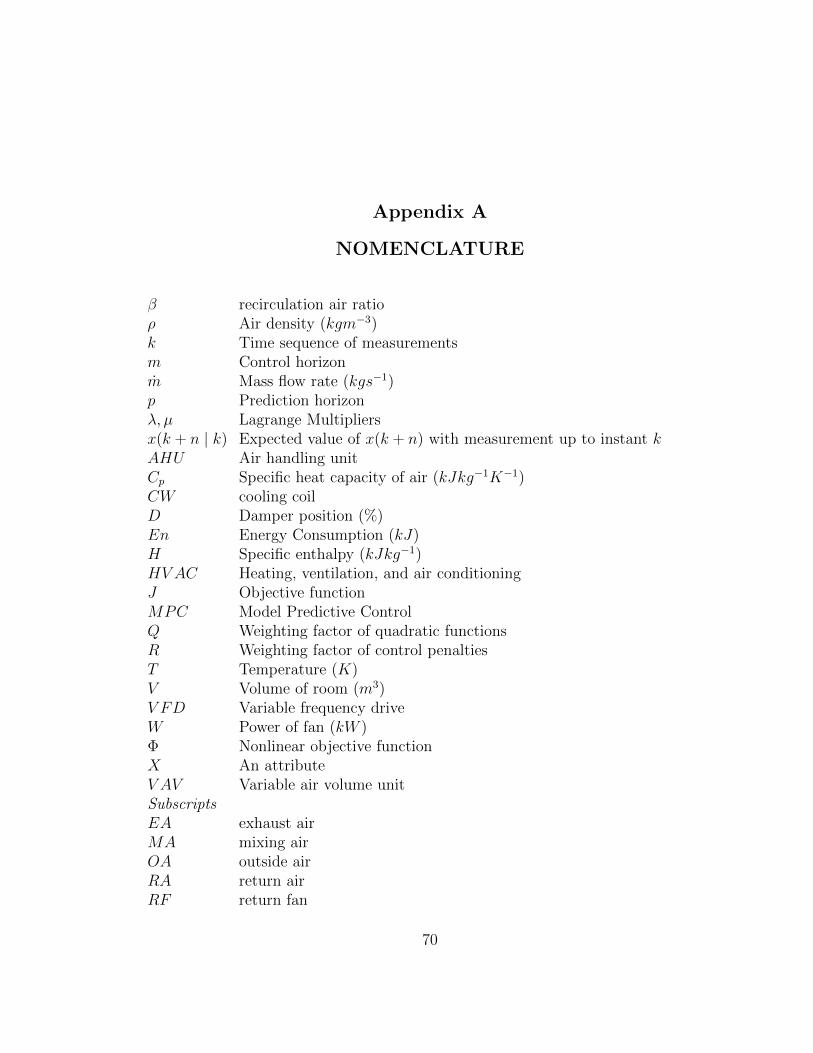
Appendix A

NOMENCLATURE

β recirculation air ratioρ Air density (kgm−3)k Time sequence of measurementsm Control horizonm Mass flow rate (kgs−1)p Prediction horizonλ, µ Lagrange Multipliersx(k + n | k) Expected value of x(k + n) with measurement up to instant kAHU Air handling unitCp Specific heat capacity of air (kJkg−1K−1)CW cooling coilD Damper position (%)En Energy Consumption (kJ)H Specific enthalpy (kJkg−1)HV AC Heating, ventilation, and air conditioningJ Objective functionMPC Model Predictive ControlQ Weighting factor of quadratic functionsR Weighting factor of control penaltiesT Temperature (K)V Volume of room (m3)V FD Variable frequency driveW Power of fan (kW )Φ Nonlinear objective functionX An attributeV AV Variable air volume unitSubscriptsEA exhaust airMA mixing airOA outside airRA return airRF return fan

70

SA supply airSF supply fand designedf air flow ratet temperaturerm roomsp set pointdis dischargeref referencezone building zone

71