UC RiversideUC Riverside Electronic Theses and Dissertations

TitleData Analysis and Query Processing in Wireless Sensor Networks

Permalinkhttps://escholarship.org/uc/item/1348s1kd

AuthorChatzimilioudis, Georgios

Publication Date2010 Peer reviewed|Thesis/dissertation

eScholarship.org Powered by the California Digital LibraryUniversity of California

UNIVERSITY OF CALIFORNIA

RIVERSIDE

Data Analysis and Query Processing in Wireless Sensor Networks

A Dissertation submitted in partial satisfaction

of the requirements for the degree of

Doctor of Philosophy

in

Computer Science

by

Georgios Chatzimilioudis

June 2010

Dissertation Committee:

Dr. Dimitrios Gunopulos, Co-ChairpersonDr. Vassilis Tsotras, Co-ChairpersonDr. Srikanth Krisnamurthy

Copyright byGeorgios Chatzimilioudis

2010

The Dissertation of Georgios Chatzimilioudis is approved:

Committee Co-Chairperson

Committee Co-Chairperson

University of California, Riverside

ABSTRACT OF THE DISSERTATION

Data Analysis and Query Processing in Wireless Sensor Networks

by

Georgios Chatzimilioudis

Doctor of Philosophy, Graduate Program in Computer ScienceUniversity of California, Riverside, June 2010Dr. Dimitrios Gunopulos, Co-ChairpersonDr. Vassilis Tsotras, Co-Chairperson

This work minimizes the cost of answering queries in wireless sensor networks. To

answer a query, data generated by the sensors needs to be collected and processed. We

optimize the cost by constructing sophisticated query trees. Queries are divided into

two categories: queries that need data from all the nodes in the network and queries

that need data from a subset of nodes only.

For the first type of queries we propose a distributed algorithm to construct

a near-optimal balanced communication tree with minimum overhead. Such a tree has

inherently minimal number of collisions during query execution, and therefore avoids

numerous retransmissions. Our algorithm outperforms previous work both in tree con-

struction overhead and in tree balance.

For the second type of queries we present methods for constructing query trees

to route and perform in-network processing of data. First, we focus on snapshot queries

and show that minimizing the problem is NP-hard. We propose a dynamic program-

ming algorithm to compute the optimal solution for small problem instances. We also

propose a low complexity, approximate, heuristic algorithm for solving larger problem

instances efficiently. Finally, we adapt the Fermat point problem (1-median problem)

iv

for a weighted graph, and propose a centralized solution that is used as heuristic in the

above algorithms.

Dealing with continuous queries of the second category, we present an optimal

distributed algorithm to adapt the placement of a single operator. Our parameter-free

algorithm finds the optimal node to host the operator with minimum communication

cost overhead. Three ideas, proposed here, make this feature possible: 1) identifying

the special, and most frequent case, where no flooding is needed, otherwise 2) limitation

of the neighborhood to be flooded and 3) variable speed flooding and eves-dropping. To

our knowledge this is the first optimal and distributed algorithm to solve the 1-median

(Fermat node) problem. In our experiments we show that for the rest of cases our

algorithm saves 30%-80% of the energy compared to previously proposed techniques.

v

Contents

List of Figures viii

List of Tables xi

1 Introduction 11.1 Introduction to Wireless Sensor Networks . . . . . . . . . . . . . . . . . 11.2 Motivating Applications . . . . . . . . . . . . . . . . . . . . . . . . . . . 21.3 Weakness of Wireless Sensor Networks . . . . . . . . . . . . . . . . . . . 41.4 Query Processing . . . . . . . . . . . . . . . . . . . . . . . . . . . . . . . 61.5 Overview of Thesis . . . . . . . . . . . . . . . . . . . . . . . . . . . . . . 7

2 Related Work 102.1 Physical Layer techniques . . . . . . . . . . . . . . . . . . . . . . . . . . 112.2 MAC Layer techniques . . . . . . . . . . . . . . . . . . . . . . . . . . . . 112.3 Network Layer techniques . . . . . . . . . . . . . . . . . . . . . . . . . . 132.4 Transport Layer techniques . . . . . . . . . . . . . . . . . . . . . . . . . 152.5 Application Layer techniques . . . . . . . . . . . . . . . . . . . . . . . . 16

3 System Model 193.1 Definition of a Wireless Sensor Network . . . . . . . . . . . . . . . . . . 193.2 Related Definitions . . . . . . . . . . . . . . . . . . . . . . . . . . . . . . 203.3 Hardware Characteristics and Energy Consumption . . . . . . . . . . . . 223.4 Estimating cost . . . . . . . . . . . . . . . . . . . . . . . . . . . . . . . . 23

4 Querying All Nodes 254.1 Introduction and Motivation . . . . . . . . . . . . . . . . . . . . . . . . . 254.2 Related Work . . . . . . . . . . . . . . . . . . . . . . . . . . . . . . . . . 304.3 System Model . . . . . . . . . . . . . . . . . . . . . . . . . . . . . . . . . 314.4 Centralized Optimization Algorithm (COPT ) . . . . . . . . . . . . . . . 334.5 Our Distributed Tree Construction Algorithm (MHS ) . . . . . . . . . . 38

4.5.1 Sequential Greedy Parent Selection . . . . . . . . . . . . . . . . . 384.5.2 Constructing an MHS Tree . . . . . . . . . . . . . . . . . . . . . 40

4.6 Experimental Evaluation . . . . . . . . . . . . . . . . . . . . . . . . . . . 444.6.1 Energy-driven Tree Construction (ETC ) . . . . . . . . . . . . . . 444.6.2 Experimental Setup . . . . . . . . . . . . . . . . . . . . . . . . . 464.6.3 Quality Of The Resulting Query Routing Tree . . . . . . . . . . 464.6.4 Tree Construction Overhead . . . . . . . . . . . . . . . . . . . . . 47

vi

4.7 A Summary . . . . . . . . . . . . . . . . . . . . . . . . . . . . . . . . . . 50

5 Instantaneously Querying A Subset Of Nodes 545.1 Introduction and Motivation . . . . . . . . . . . . . . . . . . . . . . . . . 555.2 Related Work . . . . . . . . . . . . . . . . . . . . . . . . . . . . . . . . . 57

5.2.1 Distributed Databases . . . . . . . . . . . . . . . . . . . . . . . . 575.2.2 Wireless Sensor Networks . . . . . . . . . . . . . . . . . . . . . . 58

5.3 Assumptions, Notation and Definitions . . . . . . . . . . . . . . . . . . . 595.4 NP-hardness . . . . . . . . . . . . . . . . . . . . . . . . . . . . . . . . . 625.5 Our Optimal Algorithm . . . . . . . . . . . . . . . . . . . . . . . . . . . 62

5.5.1 Our Heuristic Algorithm . . . . . . . . . . . . . . . . . . . . . . . 665.5.2 Optimization by Forcing Deep Trees . . . . . . . . . . . . . . . . 71

5.6 Branch And Bound Heuristic . . . . . . . . . . . . . . . . . . . . . . . . 735.7 Hybrid algorithm . . . . . . . . . . . . . . . . . . . . . . . . . . . . . . . 765.8 Evaluation . . . . . . . . . . . . . . . . . . . . . . . . . . . . . . . . . . . 77

5.8.1 Naive Algorithm . . . . . . . . . . . . . . . . . . . . . . . . . . . 785.8.2 Element Exchange . . . . . . . . . . . . . . . . . . . . . . . . . . 795.8.3 Experiments . . . . . . . . . . . . . . . . . . . . . . . . . . . . . 80

5.9 Summary and Conclusion . . . . . . . . . . . . . . . . . . . . . . . . . . 85

6 Continuously Querying A Subset Of Nodes 866.1 Overview and Motivation . . . . . . . . . . . . . . . . . . . . . . . . . . 876.2 Related Work . . . . . . . . . . . . . . . . . . . . . . . . . . . . . . . . . 916.3 Distributed Fermat Node Search: Preliminaries . . . . . . . . . . . . . . 936.4 Our Distributed Fermat Node Search Algorithm . . . . . . . . . . . . . 97

6.4.1 Candidate Nodes . . . . . . . . . . . . . . . . . . . . . . . . . . . 976.4.2 Calculating All Candidate Distance Combinations . . . . . . . . 986.4.3 No Flooding Cases . . . . . . . . . . . . . . . . . . . . . . . . . . 996.4.4 Flooding Radius . . . . . . . . . . . . . . . . . . . . . . . . . . . 1006.4.5 Flooding Speed . . . . . . . . . . . . . . . . . . . . . . . . . . . . 1026.4.6 The dFNS algorithm . . . . . . . . . . . . . . . . . . . . . . . . . 1036.4.7 Optimality of dFNS . . . . . . . . . . . . . . . . . . . . . . . . . 105

6.5 Initial Operator Placement . . . . . . . . . . . . . . . . . . . . . . . . . 1066.6 Experimental Evaluation . . . . . . . . . . . . . . . . . . . . . . . . . . . 1076.7 Summary . . . . . . . . . . . . . . . . . . . . . . . . . . . . . . . . . . . 118

7 Conclusions 119

Bibliography 121

vii

List of Figures

1.1 . . . . . . . . . . . . . . . . . . . . . . . . . . . . . . . . . . . . . . . . . 31.2 Energy harvesting for battery-less nodes . . . . . . . . . . . . . . . . . . 41.3 Voltree monitoring application [167], a WSN application that greatly ben-

efits from energy-efficient query routing trees . . . . . . . . . . . . . . . 5

4.1 Example of a sensor network with its possible implicit communication links 264.2 A First-Heard-From tree, shown by the bold edges, for a 4x4 grid network 274.3 A COPT solution. COVCOPT = 2.43 . . . . . . . . . . . . . . . . . . . . 384.4 An MHS solution. COVCOPT = 3.01 . . . . . . . . . . . . . . . . . . . . 434.5 An ETC solution. COVCOPT = 4.67 . . . . . . . . . . . . . . . . . . . . 454.6 Grid network. Balance of tree . . . . . . . . . . . . . . . . . . . . . . . . 484.7 Grid with diagonals network. Balance of tree . . . . . . . . . . . . . . . 484.8 Random network. Balance of tree . . . . . . . . . . . . . . . . . . . . . . 484.9 Grid network. Balance per tree level . . . . . . . . . . . . . . . . . . . . 494.10 Grid with diagonals network. Balance per level . . . . . . . . . . . . . . 494.11 Random network. Balance per tree level . . . . . . . . . . . . . . . . . . 494.12 Grid network. Maximum energy of a node . . . . . . . . . . . . . . . . . 514.13 Grid with diagonals network. Maximum energy . . . . . . . . . . . . . . 514.14 Random network. Maximum energy of a node . . . . . . . . . . . . . . . 514.15 Grid network. Total energy of network . . . . . . . . . . . . . . . . . . . 524.16 Grid with diagonals network. Total energy . . . . . . . . . . . . . . . . . 524.17 Random network. Total energy of network . . . . . . . . . . . . . . . . . 52

5.1 An instance of a Sensor Network . . . . . . . . . . . . . . . . . . . . . . 635.2 The optimal query evaluation tree given by the DPopt algorithm . . . . 635.3 The query evaluation tree given by the Naivealgorithm . . . . . . . . . . 645.4 Another instance of a Sensor Network . . . . . . . . . . . . . . . . . . . 675.5 Query plan produced by Phase 2 for evaluation tree of Figure 5.7 . . . . 675.6 Query plan produced by by Phase 2 for evaluation tree of Figure 5.8 . . 685.7 Evaluation tree returned from Phase 1 without the optimization for net-

work in Figure 5.4 . . . . . . . . . . . . . . . . . . . . . . . . . . . . . . 695.8 Evaluation tree returned from Phase 1 with the optimization for network

in Figure 5.4 . . . . . . . . . . . . . . . . . . . . . . . . . . . . . . . . . 705.9 The general Fermat Point for triangle uvq in Euclidian space is at the

X mark denoted as EFP . The best node f to place the intersectionoperator however is not even close. . . . . . . . . . . . . . . . . . . . . . 75

viii

5.10 Experiments on J-Sim with randomly generated data points. . . . . . . 775.11 Experiments on J-Sim with spatially correlated data points. . . . . . . . 785.12 Experiments no objects were used and selectivity was constant . . . . . 815.13 Experiments no objects were used and selectivity was constant. The

selectivity factor has values ranging from .3 to .9 . . . . . . . . . . . . . 825.14 Experiments with randomly generated data points. . . . . . . . . . . . . 835.15 Experiments with spatially correlated data points. . . . . . . . . . . . . 84

6.1 Example of optimal operator placement: (a) Data flow during query ex-ecution before the operator placement is optimized, and (b) data flowduring query execution after the operator placement is optimized. TheFermat node is an external node. The cost represents the cost of ourobjective function, not the actual communication cost. . . . . . . . . . . 88

6.2 Example of optimal operator placement: (a) Data flow during query ex-ecution before the operator placement is optimized, and (b) data flowduring query execution after the operator placement is optimized. TheFermat node is a datanode. The cost represents the cost of our objectivefunction, not the actual communication cost. . . . . . . . . . . . . . . . 88

6.3 GIG [3] is not an optimal algorithm. An example where GIG missesthe optimal operator placement (f). This happens because the distancesfrom candidate nodes to the datanodes are overestimated. . . . . . . . . 101

6.4 Number of nodes involved in the flooding process (minimum, average andmaximum value) using the same load for each datanode. When lines aremissing it means there were no simulation runs possible for the combina-tion of k and h values. . . . . . . . . . . . . . . . . . . . . . . . . . . . . 108

6.5 Number of nodes involved in the flooding process (minimum, averageand maximum value) using the variable load for each datanode. Whenlines are missing it means there were no simulation runs possible for thecombination of k and h values. . . . . . . . . . . . . . . . . . . . . . . . 108

6.6 Number of candidate nodes that report to the leader node. The lesscandidates the less communication needed. Beneath the x-axis the group[0,4] is divided into more detailed groups to show the distribution for dFNS.110

6.7 Quality of the first candidate node encountered while flooding (or thebest of the first set). Quality is expressed by dividing the hosting cost ofthe actual Fermat node to the first candidate. The closer the ratio is to1 the better the variable speed flooding function of the algorithm used. . 111

6.8 Quality of first candidate node when datanodes have variable data loads.Comparison of variable speed flooding functions. . . . . . . . . . . . . . 111

6.9 Total energy consumed (minimum, average and maximum value) for ex-periments with the same load for every source. When lines are missingit means there were no simulation runs possible for the combination of kand h values. . . . . . . . . . . . . . . . . . . . . . . . . . . . . . . . . . 113

6.10 The maximum energy consumed by a single node (minimum, average andmaximum value) for experiments with the same load for every source.When lines are missing it means there were no simulation runs possiblefor the combination of k and h values. . . . . . . . . . . . . . . . . . . . 113

6.11 Total energy consumed (minimum, average and maximum value). Whenlines are missing it means there were no simulation runs possible for thecombination of k and h values. . . . . . . . . . . . . . . . . . . . . . . . 114

ix

6.12 The maximum energy consumed by a single node (minimum, averageand maximum value). When lines are missing it means there were nosimulation runs possible for the combination of k and h values. . . . . . 114

6.13 Total energy consumed (minimum, average and maximum value) only forsimulation runs that needed to use flooding in order to find the Fermatnode. When lines are missing it means there were no simulation runspossible for the combination of k and h values. . . . . . . . . . . . . . . 116

6.14 The maximum energy consumed by a single node (minimum, average andmaximum value) only for simulation runs that needed to use flooding inorder to find the Fermat node. When lines are missing it means therewere no simulation runs possible for the combination of k and h values. 116

x

List of Tables

5.1 Notation . . . . . . . . . . . . . . . . . . . . . . . . . . . . . . . . . . . . 615.2 Dynamic Programming matrix C for DPopt . . . . . . . . . . . . . . . . 655.3 Algorithms to be compared . . . . . . . . . . . . . . . . . . . . . . . . . 80

6.1 Percentage of simulation runs where a datanode is the optimal node toplace the operator and thus no flooding is needed . . . . . . . . . . . . . 117

xi

Chapter 1

Introduction

1.1 Introduction to Wireless Sensor Networks

Networks of small devices equipped with sensing, computing and communica-

tion ability are conceivable, as new fabrication and integration technologies have reduced

the cost and size of micro-sensors, micro-processors and wireless interfaces. Sensor de-

vices are tiny computers, often as small as a coin or a credit card, featuring a low

frequency processor, an on-chip flash memory for local storage, a wireless radio for com-

munication, on-chip sensors, and an energy source such as AA batteries, solar panels

[186], energy harvesting [167] or energy scavenging modules [140].

Apart from the technological hardware advances that made WSN possible, a

great amount of ongoing research has given WSNs a set of unique charactristics that

make them the next multi-prurpose tool for a wide range of tasks. Each node has the

ability to sense elements of its environment, perform simple computations, and com-

municate either among its peers or directly to an external observer. A sensor network

normally constitutes a wireless ad-hoc network, meaning that the sensors organize them-

selves in a network where data can be communicated from one node to any other over

1

multi-hop routes. Sensor nodes are able to organize themselves dynamically in a net-

work topology while coping with node failures or node displacement/mobility. This great

feature, together with the on-board energy source of each sensor, allows for unattended

operation, operation in harsh environmental conditions, applications where sensor nodes

are mobile and for large scale of deployment. To the versatility of the WSN adds the

ability to deploy heterogenous type of nodes.

These systems promise to revolutionize biological, earth, and environmental

monitoring applications, providing data at granularities unrealizable by other means.

Large-scale deployments of Wireless Sensor Networks (WSNs) have already emerged in

environment and habitat monitoring [6, 161, 186], industrial process monitoring and

control [137, 96, 77], healthcare applications [6, 114, 100, 75, 122, 101], machine and

structural health monitoring [6, 158, 92, 119], home and building automation [6, 71],

urban monitoring [138, 23, 124], vehicular monitoring and traffic control [141, 52, 25].

1.2 Motivating Applications

Below, we describe the applicability of wireless sensor networks with some real

life examples.

Example 1 - People-Centric Sensing: People-centric sensing [23], aims to

support sensor-enabled applications that engage the general public through the use of

their own personal mobile devices. The recent miniaturization and integration of sensors

into popular consumer mobile devices (e.g., iPhone, HTC Touch Pro) has enabled a

myriad of new sensor based applications for personal, social and public sensing.

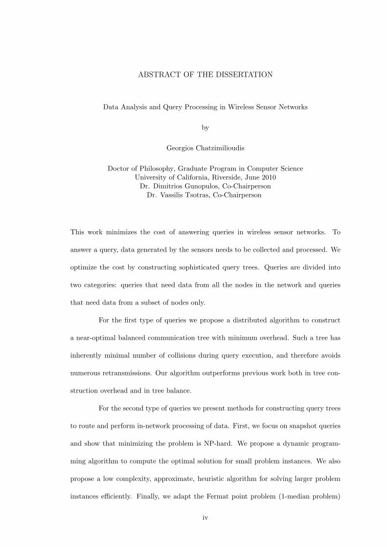
Figure 1.2, illustrates an example of a people-centric sensing scenario where

cyclists journey through the main streets of a city [120]. Each cyclist is equipped with a

2

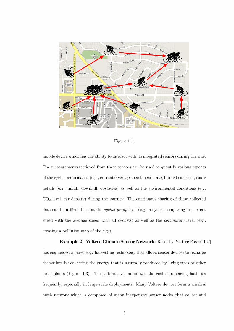
Figure 1.1:

mobile device which has the ability to interact with its integrated sensors during the ride.

The measurements retrieved from these sensors can be used to quantify various aspects

of the cyclic performance (e.g., current/average speed, heart rate, burned calories), route

details (e.g. uphill, downhill, obstacles) as well as the environmental conditions (e.g.

CO2 level, car density) during the journey. The continuous sharing of these collected

data can be utilized both at the cyclist-group level (e.g., a cyclist comparing its current

speed with the average speed with all cyclists) as well as the community level (e.g.,

creating a pollution map of the city).

Example 2 - Voltree Climate Sensor Network: Recently, Voltree Power [167]

has engineered a bio-energy harvesting technology that allows sensor devices to recharge

themselves by collecting the energy that is naturally produced by living trees or other

large plants (Figure 1.3). This alternative, minimizes the cost of replacing batteries

frequently, especially in large-scale deployments. Many Voltree devices form a wireless

mesh network which is composed of many inexpensive sensor nodes that collect and

3

Figure 1.2: Energy harvesting for battery-less nodes

report data on temperature, humidity, wind speed and direction. Data collected by

the nodes is recursively transmitted from each node to its neighbors (i.e., forming a

query routing tree) until these measurements reach a central base station that records

the data for further analysis. Such networks have already been deployed by the United

States Department of Agriculture (USDA) at 5 different sites [167]. These networks

complement the USDA Forest Service’s Remote Automated Weather Stations network.

Such applications deploy Query Routing Tree structures as a primitive mechanism for

percolating query results to nodes that query the network.

1.3 Weakness of Wireless Sensor Networks

Probably the weakest point of wireless sensor networks is the limited energy

source of its nodes. The autonomy of the sensor nodes comes with a price: commu-

nication over the wireless channel needs a lot of energy. It is well established that

communicating over the radio in a WSN is the most energy demanding factor among

all other functions, such as storage and processing [111, 184, 176, 112, 182]. The energy

4

Figure 1.3: Voltree monitoring application [167], a WSN applicationthat greatly benefits from energy-efficient query routing trees

consumption for transmitting 1 bit of data using the MICA mote [39] is approximately

equivalent to processing 1000 CPU instructions [111].

In addition, the wireless channel is unreliable due to collisions, node failures,

obstacles and hostile environment parameters, causing many packets to get dropped

[6, 189]. Collisions between data packets happen when multiple neighboring sensor

nodes attempt to access the shared wireless channel and is the main cause of dropped

packets [79]. Every dropped packet needs to be retransmitted adding to the energy

consumption.

Increasing the lifetime of a WSN is essential, thus WSN applications have

to be founded on the premise of energy-conscious algorithms. A sensor network is

operational when its nodes are able to sense and to communicate with their neighboring

nodes. A node can perform these functions as long as its energy source is not depleted.

The duration for which a sensor network is operational is called lifetime and it can be

estimated theoretically. Depending on the application it is defined by the time it takes

for the first x nodes to get depleted [51]. Minimizing the maximum energy per node

5

prolongs the time for the first node to get depleted. The time it takes for a number of

nodes to get depleted can be prolonged balancing the maximum energy per node and

the total energy consumed in the network.

Supplementary approaches to cope with the energy challenge have been pro-

posed at virtually all layers of the sensing device stack ranging from the hardware

layer [134, 39] to the operating system layer [74], the programming language [60], the

network layer [190] and the data management layer (e.g., storage [184, 115], compres-

sion [43, 148], query processing [111, 176, 146, 112, 182, 36, 30, 31] and prediction [63]).

A decisive variable for prolonging the longevity of a WSN is to minimize the utilization

of the wireless communication medium. Therefore, a general theme in the above men-

tioned approaches is to reduce the number and size of messages communicated between

sensors in order to minimize the use of the radio transceiver.

1.4 Query Processing

Wireless sensor networks can be viewed as a network of tiny distributed databases,

where data needs to be collected and processed in order to satisfy a user request/query.

In wireless sensor network applications, like the ones discussed above, the user requests

information through one of the nodes. To answer a query, data generated by the sen-

sors needs to be collected and processed. The processing is done centralized on the

basestation or distributed on the nodes of the network (in-network processing).

Sophisticated query processing can greatly prolong the lifetime of the WSN.

Routing of data from their sources to their processing locations allows for great reduction

in the number and size of messages communicated between sensors. There is a vast

amount of research already undertaken in this respect. In this thesis new problems

6

are addressed and solved and new efficient solutions are proposed for already known

problems. The proposed techniques are categorized according to the type of query they

optimize.

We can distinguish between queries that only need data from a subset of nodes

in the network and queries that need data from all the nodes in the network. A popular

application field for the former type ar geographical applications, where queries require

information from several regions. Such queries are called multi-predicate queries (MPQ)

and this term will be used throughout this work. An instance of such a query in a moving

object monitoring application would be the following: “What objects passed through

region A, B, and C?”. The latter type can be found mainly in environmental monitoring

applications and is called henceforth All Node Queries ANQ. “What is the temperature

of every room in the building?”.

We can also distinguish between queries that need to be answered once (snap-

shot queries) and queries that need to be answered continuously as new data is being

collected from the nodes (continuous queries). “What is the temparature read by each

sensor at timepoint T” and “What objects passed through region A, B and C so far?”

would be instances of snapshot queries. Respectively, “What is the temparature read by

each sensor from this timepoint for the next 24 hours” and “What objects pass through

regions A, B and C for the next 7 days” are instances of continuous queries.

1.5 Overview of Thesis

The main goal of this work is to optimize query execution in the face of com-

munication cost. We optimize three kinds of queries: 1) All-Node Queries (ANQ), 2)

snapshot Multi-Predicate Queries (MPQ), and 3) continuous Multi-Predicate Queries.

7

Optimizing All-Node Queries we propose a distributed algorithm to construct

a balanced communication tree that will serve in gathering data from the network nodes,

with the base-station as the final receiver. Our algorithm constructs a near-optimally

balanced communication tree with minimum overhead. The balancing of the node de-

grees, at each level of the tree, results in the minimization of hot-spots and thus packet

collisions, that would otherwise require numerous retransmissions and reduce the life-

time of the network. We compare our simple distributed algorithm against previous

work and a centralized solution and show that for most network layouts it outperforms

competition and achieves tree balance very close to the centralized algorithm. It also

has the smallest energy overhead possible to construct the tree, increasing the lifetime

of the network even more.

Optimizing snapshot Multi-Predicate Queries we propose a centralized algo-

rithm that minimizes the cost of answering snapshot multi-predicate queries in wireless

sensor networks. The important class of multi-predicate queries in horizontally or verti-

cally distributed databases is addressed. We show that minimizing the communication

cost for multi-predicate queries is NP-hard and we propose a dynamic programming al-

gorithm to compute the optimal solution for small problem instances. We also propose

a low complexity, approximate, heuristic algorithm for solving larger problem instances

efficiently and running it on nodes with low computational power (e.g. sensors). Finally,

we present a variant of the Fermat point problem where distances between points are

minimal paths in a weighted graph, and propose a centralized solution. An extensive

experimental evaluation compares the proposed algorithms to the best known technique

used to evaluate queries in wireless sensor networks and shows improvement of 10% up

to 95%. The low complexity heuristic algorithm is also shown to be scalable and robust

to different query characteristics and network size.

8

Optimizing continuous Multi-Predicate Queries we present an optimal dis-

tributed algorithm to adapt the placement of a single operator in high communication

cost networks, such as a wireless sensor network. Our parameter-free algorithm finds

the optimal node to host the operator with minimum communication cost overhead.

Three techniques, proposed here, make this feature possible: 1) identifying the special,

and most frequent case, where no flooding is needed, otherwise 2) limitation of the

neighborhood to be flooded and 3) variable speed flooding and eves-dropping. When no

flooding is needed the communication cost overhead for adapting the operator placement

is negligible. In addition, our algorithm does not require any extra communication cost

while the query is executed. In our experiments we show that for the rest of cases our

algorithm saves 30%-85% of the energy compared to previously proposed techniques. To

our knowledge this is the first optimal and distributed algorithm to solve the 1-median

(Fermat node) problem.

The dissertation is structured as follows: Chapter 1 describes in detail the

work done regarding the optimization of all-node queries. Snapshot and continuous

Multi-predicate queries are optimized in Chapters 2 and 3 respectively. In all following

Chapters the work is devided in introduction and motivation, related work, system

model definition, the solutions proposed and its experimental evaluation, concluding

with a summary.

9

Chapter 2

Related Work

Power conservation mechanisms have been proposed virtually at all layers of

the traditional layered sensor communication stack. All these approaches attempt to

decrease the energy consumption with two basic techniques: i) by disabling/hibernating

the radio transceiver during periods of inactivity, and ii) by improving the sensor nodes

operation (e.g., voltage scaling, employing multiple power levels). Most of these tech-

niques are complementary to the techniques described in this paper while the rest come

with their own trade-offs as we will show shortly.

In this section, we present an elaborate overview of techniques, that decrease

communication related power consumption in WSNs. Following the widely adopted

ISO/OSI communication stack [98] as categorization criteria, allows to accurately cap-

ture the main focus and limitations of each presented technique. We shall also refer to

cases of cross-layer optimizations individually. For the remainder of this section, we will

present the universe of techniques in a bottom-up manner, starting from the physical

layer and moving up to the application layer where our own algorithms belong. We

omit the Presentation and Session layers of the typical ISO/OSI stack as none of the

10

presented techniques addresses these layers specifically.

2.1 Physical Layer techniques

This layer relates to the low-level sensor device hardware (circuitry, MCU,

transceiver, etc) thus the opportunity for software level power management is fairly

limited. Yet, there are a few works [20, 69, 152] that look at individual and local power

management optimizations.

Examples of these techniques are the Dynamic Voltage Scaling [20] and Em-

bedded power supply for low power Digital Signal Processor [69] which are effective tech-

niques for reducing the energy consumption of the CPU. The goal of these approaches

is to adapt the processors power supply and operating frequency to match any given

computation load without degrading performance. Dynamic Power Management [152]

is another work that utilizes different power models to shut down various components

(e.g., radio transceiver, CPU) when these are not required to operate. All of the above

techniques, and generally any local power conservation mechanism at the physical layer,

are supplementary to the algorithms presented in this dissertation.

2.2 MAC Layer techniques

The Medium Access Control (MAC) layer facilitates the transfer of messages

to and from the physical layer. Most of the protocols developed for the MAC layer

deploy explicit mechanisms to avoid collisions when multiple sensor nodes attempt to

access a shared channel. Most of the sensor network related works presented in this layer

[126, 177, 155, 151] minimize energy consumption by minimizing collisions and overall

usage of the shared access medium.

11

The Coordinated Power Conservation algorithm (CPC) [155] is an example of a

MAC-layer power management protocol that coordinates the sleeping intervals of sensor

nodes with the aid of a backbone. CPC starts out by selecting a set of backbone nodes

as CPC servers. Next all CPC clients that run on non-backbone nodes, request to turn

the transceiver of the sensor node off when there is no communication activity, in order

to conserve power and extend network lifetime. CPC servers running on backbone nodes

serve as coordinators to synchronize sleeping schedules of nodes within their coverage

areas. This solution is orthogonal to our problem and can be used in parallel to the

solutions we give to the problem of minimizing communication cost.

Power-aware Multi-Access Protocol with Signaling (PAMAS) [151] is another

MAC-layer power management protocol that utilizes two independent radio channels

in order to avoid overhearing among neighboring nodes. Battery power is saved by in-

telligently turning-off sensor nodes that are not in active transmission. On the other

hand, the popular Sensor-MAC (S-MAC) [177], utilizes a synchronization scheme that

allows sensor nodes to realize periodic listening and sleeping during busy periods (i.e.,

when transmission from other nodes is detected). Furthermore, S-MAC consists of two

additional components that handle: i) collision and overhearing avoidance by allowing

sensor nodes, receiving control packages not destined, to them go to sleep, and ii) mes-

sage passing by segmenting long messages into smaller ones and transmitting in bursts

(i.e., RTS/CTS control messages are not used for each fragment). S-MAC has been

further enhanced in [126] to minimize the end-to-end delay. Both PAMAS and S-MAC

achieve high energy savings by allowing sensor to sleep periodically.

However, none of these approaches considers the underlying topology of the

sensor network, intra-sensor relationships and high-level query semantics. In particular,

these techniques do not consider the workload of a continuous query, rather they assume

12

a random variable workload. For general queries, we propose an algorithm to minimize

collisions by constructing a near balanced routing tree. Nevertheless, since the S-MAC

proocol has been succesfully integrated in TinyOS [68] as one of the primary MAC

protocols, these techniques extend the power management capabilities of our algorithms

inherently.

Sensornet Protocol (SP) [133], introduces a unified link level abstraction that

is part of the sensor network architecture proposed in [40]. Specifically, SP provides

shared neighbor management and message pool interfaces that allow network protocols

to exchange messages efficiently and choose neighbors wisely without concentrating on

link specifics. To accomplish this, these interfaces encapsulate the mechanisms of the

particular link and physical layers that operate below the Sensornet Protocol. The

authors show that various link layer protocols can be expressed in terms of SP and

subsequently mapped efficiently to various link level power management mechanisms.

2.3 Network Layer techniques

This layer is responsible for delivering packets from a source node to a des-

tination node through some routing mechanisms. In WSNs, routing is accomplished

using multi-hop messages, thus many mechanisms in this layer attempt to discover op-

timal routing paths for energy efficient delivery of messages through intermediate hosts

[72, 64, 42]).

The Power-Aware Routing (PAR) [64] technique is a routing policy that bal-

ances the overall power in the network by discovering routes that consume the least

possible energy. Since in a non-uniform network the majority of nodes do not consume

power in an identical fashion, PAR favors nodes with larger power reserves. Another

13

technique is the Minimum Connected Dominating Sets (MCDS) routing algorithm [42]

which employs a virtual backbone that provides shortest paths for routes, as well as

route updates in cases of node movements, in order to minimize the overall energy re-

quired for routing multi-hop packets. Both PAR and MCDS approaches assume an a

priori established query routing tree.

Both PAR and MCDS approaches assume an a priori established query routing

tree. Any optimizations suggested by both approaches does not alter the state of the

query routing tree. On the other hand, our algorithms differ from these approaches as

they reconstruct the tree in order to minimize collisions or dataloads transferred prior

to any further optimizations. Certain modules of PAR and MCDS (e.g., shortest path

discovery) can be used in conjuction with our algorithms in order to achieve even more

energy savings.

In Modular Network Layer [53] the authors decompose the network layer into

smaller components that can be used by several protocols in parallel. This network layer

operates on top of the popular Sensornet link-layer Protocol [133]. The intuition behind

their approach is that the majority of network protocols have many commonalities.

Encapsulating these commonalities and exposing them as service interfaces enables faster

development of new protocols and run-time sharing of components. The authors evaluate

their approach and find that the Modular Network Layer can reduce both the memory

footprint and lines of code of network protocols that run concurrently. Consequently,

this work is supplementary to our work, as our protocols could have been implemented

using this intermediate framework rather than in a standalone.

14

2.4 Transport Layer techniques

The transport layer is responsible for the transfer of messages between two or

more end systems using the network layer. One of the main objectives of the transport

layer is the reliable and cost effective delivery of transferred messages between applica-

tions. The evolution of the techniques in this layer has been severely hampered by the

fact that sensor networks feature node failures and collisions making reliable and cost

effective communication often impossible.

One of the few works that addresses the above issues is the TCP-Probing

communication protocol [165], which introduces the concept of a probe cycle instead of

standard TCP re-transmissions, congestion window and threshold adjustments. During

probe cycles, data transmission is suspended and only probe segments are sent. The

proposed scheme achieves high throughput performance at the same time decreasing

the overall energy consumption for transmission. This is done without damaging the

end-to-end characteristics of TCP.

Flush [91] is another transport layer protocol for multi-hop wireless networks.

Flush provides end-to-end reliability, reduces transfer time and adapts to time-varying

network conditions. To accomplish these properties, Flush uses end-to-end acknowl-

edgments, implicit snooping of control information and a rate-control algorithm that

operates at each hop along a flow.

In contrast to the probe cycles of TCP-Probing and end-to-end acknowledg-

ments of Flush, our algorithms either straightforwardly reduce collisions or reduce the

effect of collisions and failures by minimizing the size of the messages to be sent. The

aforementioned techniques would introduce further delays as well as more energy waste

since the sensors would have to exchange more messages in order to synchronize.

15

2.5 Application Layer techniques

The main objective of this high level layer is to exploit the semantics of the

network or application and low-level data in order to optimize the network structure

among nodes and boost power management. Consequently, this layer has implicit inter-

actions with lower levels of the communications stack (often referred to as cross-layer

optimizations [7]). The techniques in this layer can be roughly classified in the follow-

ing: i) local techniques, in which low-level data semantics dictate the reaction of the

application, and ii) cluster-based techniques, in which the reaction of the application is

dictated by the cluster semantics (e.g., network proximity).

In the first category, Application-Driven Power Management for Mobile Com-

munication [94] and Adaptive Energy Conserving Routing (AdECoR) [172], are examples

of application-layer techniques that enable the dynamic power configuration of the com-

munication device. The intuition behind this approach is that although switching-off

the communication device may result in energy conservation, it may also introduce de-

lays in the network. AdeCoR attempts to find a trade-off between energy conservation

and latency by utilizing application-level information and adjusting the sleep duration

of the communication device. AdECoR differs from our work as its application-level

information does not include the high level query semantics. Furthermore, the concept

of introducing delays in order to conserve power is not acceptable in our problem setup

as we assume that queries have specific response time requirements that must be met.

In addition, various data acquisition frameworks (e.g. [111, 112, 176, 102])

have been proposed that aim to minimize the utilization of the wireless communication

medium only by minimizing the data sent or the time that the tranceiver is operating.

Those techniques will be examined in more detail in the following chapter that detail

16

our algorithms.

The second class of application layer techniques includes those techniques that

use clustering mechanisms. Works like LEACH [72], PEGASIS [106] and PEDAP [187]

minimize the overall energy consumption in WSNs by rotating the cluster head nodes

that collect data in a random manner. This rotation allows the distribution of the energy

load evenly among the sensor nodes in the network without draining the energy resources

of an individual sensor node. Another example is Geographical Adaptive Fidelity (GAF)

[173], which obtains location information using the Global Positioning System (GPS)

in order to connect sensor nodes to a virtual grid (i.e., a semantic overlay based on

geographical proximity). It then saves energy by keeping sensor nodes located in a

particular grid area in sleeping state. The sleeping schedule uses a turn-based approach

that aims to balance the load incurred on each sensor. Finally, SPAN [32] builds on the

observation that when a region of a shared-channel has a sufficient density of nodes, only

a small number of them needs to be present at any time to forward traffic for active

connections. To accomplish this, SPAN utilizes a distributed, randomized algorithm

that allows sensors to make local decisions as to when sleeping is appropriate. GAF and

SPAN, take advantage of global information to preserve energy. Both approaches switch

off some sensors based on some application level parameters and force other sensors to

seek alternate routing paths.

GPS and SPAN, like our work, take advantage of global information to pre-

serve energy. Both approaches switch-off some sensors based on some application-level

parameters and force other sensors to seek alternate routing paths. However, switching-

off some sensors means that they cannot participate in a given query and as a result,

valuable results may be lost even for shorts period of time. LEACH differs from our

approach since all nodes that participate in a given query are considered equal peers

17

and none plays a separate role (e.g., cluster head) nor has more energy reserves than

others.

18

Chapter 3

System Model

3.1 Definition of a Wireless Sensor Network

For this work, the mathematical abstraction of a sensor network is that of an

undirected graph. Nodes of the graph represent sensors in the network while edges

represent bi-directional communication links. The latter are characterized by two nodes

having the ability to send information to one another and may be defined as having

noisy properties. Nodes have computational ability that is physically limited but these

limits will not be considered restrictive for the algorithms discussed. Nodes are able to

sense physical properties (e.g. temperature, magnetic field) at their location.

Let V denote a set of n sensing devices {v1, v2, ..., vn} in a wireless sensor

network. Now let G = (V,E) denote the network graph that represents the implicit

network edges E of the nodes in V . The edges in E are implicit, because there is no

explicit connection between adjacent sensor nodes, but nodes are considered neighbors

if they are within communication range.

The simplification, that communication is possible between two nodes if their

physical separation is less than the maximum communication distance R, will be used.

19

A connected graph is one wherein any two nodes have an uninterrupted path between

them following edges of the graph. In the physical context, this means that any two

nodes can communicate with a finite number of hops between them. Only connected

graphs are considered - plural subgraphs with no communication link among them can be

considered independently for this work. Since our nodes have a restricted communication

range R, data will have to travel over a multi-hop path toward the querying node. A

routing tree T is created connecting every node. The querying node q is the root of this

tree and receives the information needed to answer the query. The tree connects all the

nodes over a multi-hop path to the sink.

3.2 Related Definitions

Let S denote a set of n sensing devices {s1, s2, ..., sn}. Assume that si (i ≤ n)

is able to acquire m physical attributes {a1, a2, ..., am} from its environment at every

discrete time instance t. This generates at each t and for each si (i ≤ n) one tuple of the

form {t, a1, a2, ..., am}. This scenario conceptually yields an n ×m matrix of readings

X:=(sij)n×m for each timestamp. This matrix is horizontally fragmented across the n

sensing devices (i.e., row i contains the readings of sensor si and X = ∪i∈nXi). Now let

G = (S,E) denote the network graph that represents the implicit network edges E of the

sensors in S. The edges in E are implicit, because there is no explicit connection between

adjacent nodes, but nodes are considered neighbors if they are within communication

range R (i.e., a fundamental assumption underlying the operation of a radio network).

A user can run queries on a wireless sensor network. Wireless sensor networks

can be viewed as a network of tiny distributed databases and queries can be posed

through a node of the network. To answer a query, data generated by the sensors needs

20

to be collected and processed. The processing is done centralized on the basestation or

distributed on the nodes of the network (in-network processing). We assume that nodes

can pose queries over the sensor network. The sensor node that issues the query Q is

called querying node and is denoted as q. We will use the terms querying node and sink

interchangeably throughout this work.

We can distinguish between queries that only need data from a subset of nodes

in the network and queries that need data from all the nodes in the network. A popular

application field for the former type ar geographical applications, where queries require

information from several regions. Such queries are called multi-predicate queries (MPQ)

and this term will be used throughout this work. We can also distinguish between queries

that need to be answered once (snapshot queries) and queries that need to be answered

continuously as new data is being collected from the nodes (continuous queries).

Continuous queries are answered in consecutive data acquisition rounds called

epochs. An epoch is a small time period in which the query is answered once, like a

snapshot query. A user specifies a continuous query Q to be evaluated once during the

interval of an epoch (denoted as e), which is the time interval after which each si (i ≤ n)

will re-compute Q.

For simplicity let us adopt a declarative SQL-like syntax (similarly to [?, ?])

to express the ideas presented in this work in brevity. For instance, the following query

declares that each sensing device should recursively collect the node identifier and the

temperature from its children every 31 seconds and communicate the results to the sink.

SELECT nodeid, temp

FROM sensors

EPOCH DURATION 31 seconds

Note that our model also supports continuous aggregate queries. For instance,

21

the following query declares that each sensing device should aggregate the average light

measurement for each room from its children every 31 seconds and communicate the

results to the sink.

SELECT roomid, AVG(light)

FROM sensors

GROUP BY roomid

EPOCH DURATION 31 seconds

In order to process queries efficiently over a Wireless Sensor Networks (WSNs),

sensors need to be organized in a Query Routing Tree T . A query routing tree is an

acyclic subset of the communication graph G (i.e., a spanning tree) which is denoted as

T = (V ′, E′), where V ′ ⊆ V and E′ ⊆ E. T can be constructed based on query seman-

tics, power consumption, remaining energy and others. A query routing tree provides

each sensor with a path over which query answers can be transmitted to the query-

ing node and allows for waking window and data reduction techniques to optimize the

energy consumption in the network. An epoch can use the same query tree T as the

previous epoch and save the overhead of tree construction. Otherwise, it can be deemed

more efficient to reconstruct or adapt the query tree for the new epoch.

3.3 Hardware Characteristics and Energy Consumption

The wireless sensor node, being a micro-electronic device, can only be equipped

with a limited power source (<0.5 Ah, 1.2 V). In sensor networks power efficiency is

an important performance metric, directly influencing the network lifetime. Application

specific protocols can be designed by appropriately trading off other performance metrics

such as delay and throughput with power efficiency.

22

Energy expenditure in data communication is far greater compared to data

processing. The example described in [135], effectively illustrates this disparity. Mixers,

frequency synthesizers, voltage control oscillators, phase locked loops (PLL) and power

amplifiers, all consume valuable power in the transceiver circuitry. This involves both

data transmission and reception. It can be shown that for short-range communication

with low radiation power (0 dbm), transmission and reception energy costs are nearly

the same.

In [149], the authors present a formulation for the radio power consumption

(Pc) as

Pc = NT (PT (Ton + Tst) + Pout ∗ Ton) +NR(PR(Ron +Rst))

where PT /PR is the power consumed by the transmitter/receiver; Pout, the output power

of the transmitter; Ton/Ron , the transmitter/receiver on time; Tst/Rst , the transmit-

ter/receiver start-up time; and NT /NR , the number of times transmitter/receiver is

switched on per unit time, which depends on the task and medium access control (MAC)

scheme used. We can further say that Ton = L/R, where L is the packet size and R the

data rate.

3.4 Estimating cost

For the objective function, that we use in our algorithms, we follow the same

energy model as Coman et al [37]. The cost of shipping data from node u to node v is

proportional to the data load wu to be shipped, and the weight of the path used. The

path weight W (u, v) is equal to the sum of the weights of all links l ∈ L that make up

path (u, v): W (u, v) =∑

l∈links(u,v)wl, where wl is the weight of the link l ∈ L. The

23

cost of shipping data from node u to node v is defined as

t(u, v) = wu ∗W (u, v)

This simplified version is used only as an objective function in our algorithm to estimate

communication cost. Note that the computation of the actual energy consumed by the

network when transmitting a message over a path is more complicated. In the network

simulator, that we used to run our experiments, the energy consumption model is much

more realistic. It also takes into account the energy consumed by the neighbors of u

and v since they also receive the packet.

To estimate the energy needed to answer a query Q over a query tree T once,

we define T (i, j) as the function that returns 1 whenever the edge (i, j) is used in the

query evaluation:

T (i, j) =

1 if communication edge (i, j) is used

0 otherwise

(3.1)

The total communication cost CQ of answering query Q will be:

CQ =

m,m∑

i=1,j=1

c ∗ T (i, j) ∗Bi (3.2)

where nodes i, j ∈ V . This does not include the cost of disseminating the query or

constructing the tree T .

24

Chapter 4

Querying All Nodes

We propose a distributed algorithm to construct a balanced communication

tree that will serve in gathering data from the network nodes, with the base-station as

the final receiver. Our algorithm constructs a near-optimally balanced communication

tree with minimum overhead. The balancing of the node degrees, at each level of the tree,

results in the minimization of hot-spots and thus packet collisions, that would otherwise

require numerous retransmissions and reduce the lifetime of the network. We compare

our simple distributed algorithm against previous work and a centralized solution and

show that for most network layouts it outperforms competition and achieves tree balance

very close to the centralized algorithm. It also has the smallest energy overhead possible

to construct the tree, increasing the lifetime of the network even more.

4.1 Introduction and Motivation

Wireless sensor networks (WSNs) are the next multi-purpose tool for a wide

range of tasks. The main characteristic that makes them so useful is the autonomy of

the nodes due to their freedom of attachment. Nodes do not need to be attached to

25

0 1 2 3

4 5 6 7

8 9 10 11

12 q 14 15

Figure 4.1: Example of a sensor network with its possible implicitcommunication links

one another in order to communicate; they communicate using radio transceivers over

wireless channel. Also, they do not need to be attached to any static energy provider;

they have batteries on board. The autonomy of the sensor nodes comes with a price:

communication needs a lot of energy and on-board batteries have limited energy sup-

plies. Further, the wireless channel in WSNs is unreliable with many dropped packets.

Collisions between data packets, when multiple sensor nodes attempt to access a shared

wireless channel, is the main cause of dropped packets. Every dropped packet needs to

be retransmitted adding to the energy consumption.

Due to the limited energy source, WSN applications have to be founded on the

premise of energy-conscious algorithms. A decisive variable for prolonging the longevity

of a WSN is to minimize the utilization of the wireless communication medium. It is well

established that communicating over the radio in a WSN is the most energy demanding

factor among all other functions, such as storage and processing [182, 111, 112, 184, 176].

In data acquisition systems for WSNs data from every node of the network

needs to be collected at a sink node. An example can be seen in Figure 1.1. The majority

of existing approaches use a Query Routing Trees (denoted as T ), which provides each

sensor with a path over which query answers can be transmitted to the querying node.

26

0 1 2 3

4 5 6 7

8 9 10 11

12 q 14 15

0 1 2 3

5 7

9 10 11

q 14 15

Figure 4.2: A First-Heard-From tree, shown by the bold edges, for a4x4 grid network

Energy-efficient query routing trees are useful in a plethora of systems such

as People-centric Sensing [23], structural monitoring [92], urban monitoring [124] and

environmental monitoring sensor networks [167, 162, 186] among others. In all of

these environments a device requests sensor data from any available neighboring device

through the establishment of an ad-hoc communication network. These adhoc links are

usually founded on the premise of a Query Routing Trees and constructing optimized

trees is of major importance in these scenarios.

T structures are usually constructed in an ad-hoc manner and therefore there

is no guarantee that the query workload will be distributed equally among all sensors.

In Figure 4.1 we can see an ad-hoc query routing tree created when each node connects

to the node that it first heard the tree construction request from. Nodes with many

incoming streams are called hot-spots. Various data acquisition frameworks (e.g. [111,

112, 176, 72, 106, 187, 102]) have been proposed that aim to minimize the utilization

of the wireless communication medium, but they only try to minimize the data sent,

the time that the transceiver is operating or alternate the root node to reduce energy

consumption around the root.

The inherent imbalance of ad-hoc query routing trees leads to data collisions

during transmission which represent a major source of energy waste. For instance in

27

[10] it is shown that the execution of a query over a node with 10 children will lead

to a 48% loss rate of data packets, while executing the same query over a node with

30 children will lead to a 56% loss rate. These figures translate into an approximately

three-fold increase in energy demand due to inevitable re-transmissions of data packets.

Consequently, unbalanced query routing trees can severely degrade the network health

and efficiency.

Balanced query routing trees have the following desirable properties: i) they

decrease collisions during data transmission, and ii) they decrease query response times

and iii) they increase system lifetime and coverage. It is shown by the authors of

[10] that constructing a balanced query routing tree T increases the lifetime of a WSN

significantly. We provide algorithms and methods to create balanced query routing trees

in a network.

We give a formal definition of balance in a query routing tree and propose a

centralized algorithm that constructs good approximation of an optimally balanced tree.

This algorithm is only used as a ground truth solution to compare against, as it has high

complexity and high communication cost for acquiring the needed network information

to run.

We devise a simple distributed algorithm that constructs a query routing tree

with minimum deviation from the optimally balanced and is very suitable for use in

wireless sensor networks. It is based on letting nodes select parents sequentially while

“snooping” the wireless channel and counting the degree of their candidate parent nodes.

When the time comes to select a parent, the node simply selects the parent with the

minimum degree. The order of parent selection amongst nodes is decided locally by each

node.

Our decentralized algorithm (MHS ) performs very close to the optimal, espe-

28

cially in networks that resemble real world sensor network layouts. In addition, the

overhead to run our algorithm is negligible compared to the baseline First Heard From

tree construction used widely in ad-hoc sensor network. The messages exchanged be-

tween nodes during the whole process are limited to the very basic ones that are needed

to connect two nodes with a hand-shake protocol. Our experimental evaluation also

shows that our algorithm is a great improvement over the previously proposed algo-

rithm [10], both in query routing tree balance achieved and in the energy overhead

imposed for construction.

Our contributions can be summarized as follows:

• We define a balanced query routing tree in a way that takes into account the

communication restrictions in a network. That allows us to decompose the bal-

anced query routing tree construction problem into a set of simpler subproblems

(Balanced Assignment Problem).

• We propose a novel distributed algorithm (MHS ) to approximate the balanced

query routing tree construction solution.

• We prove that MHS has the minimum possible communication overhead.

• We show through simulations thatMHS improves the balance of the resulting query

routing tree significantly over the previously proposed algorithm and for real world

networks even performs as good as the centralized algorithm.

In the next sections we discuss related work (Section 2) present the system

model and the definition of the balanced query routing tree problem (Section 3). In

Section 4.4 we analyze the problem, decompose it into a set of simpler subproblems and

present our centralized algorithm. The description of the novel distributed algorithm

29

follows in Section 4.5 to finish with the experimental evaluation (Section 4.6) and a short

summary (Section 4.7).

4.2 Related Work

A distributed algorithm to create a query routing tree without the assumption

that every node can transmit directly to the sink, has been proposed in [174]. Their

algorithm balances the data load to be transmitted from one tree level to the next.

The goal is to balance the data received and relayed by each node in the network. The

energy savings by this work are mostly theoretical since they do not deal with collisions

occurring from many nodes trying to communicate with the same parent. As shown by

Andreou et al. [10] the energy loss due to hot-spots in the tree can not be neglected.

To the best of our knowledge the only previous work balancing a tree in order to

minimize collisions is the work of Andreou et al. [10]. The algorithm they propose, called

ETC, constructs an initial temporal unbalanced tree and then lets nodes communicate

back and forth in order to reorganize and balance the tree. ETC adds a significant

overhead in order to balance the tree: the number of packets exchanged is high. The

most important downfall for ETC is that balancing is based on a global branching factor

that in many network topologies results in a tree that is far from optimally balanced.

We propose a distributed algorithm (MHS ) that constructs a query routing

tree with minimum hot-spots (balanced tree). This translates in a reduced number of

packet collisions during query execution. MHS has significantly reduced overhead for

constructing a tree and the resulting tree deviates far less from the optimally balanced

tree when compared to ETC as is shown in our experiments.

30

4.3 System Model

In this section we formalize our system model and the basic terminology that

will be utilized in the subsequent sections. We give formal definitions and proposition

that we use in our algorithms and use to define the balanced tree construction problem.

The querying node q is the root of the query tree T and receives the information

needed to answer the query. The tree connects all the nodes over a multi-hop path to

the sink. The nodes inside a tree can be divided in tree levels. A level is defined by how

far the nodes are from the root. The level of the root is zero.

Proposition 1 Given a tree T = (V,A) and two nodes u, v ∈ V that are adjacent,

(u, v) ∈ A, and at levels lu and lv respectively, it must be lu 6= lv and |lu − lv| = 1

The node at the lower level (min{lu, lv}) is called parent, and the other is called

its child. An edge (u, v) ∈ A is called an adoption of u from v.

Definition 2 Given a graph G(V,E) and a sink q, the set of candidate parents of node

c ∈ V , for constructing a tree T = (V,A), is the set P ⊂ V of nodes p for which an edge

(c, p) ∈ E exists and for the shortest hop distance lc from c to the sink q and lp from c

to q it holds that lp = lc − 1.

Given a graph G and a sink q, if we construct a tree T by connecting each

node only to one of its candidate parents, it is guaranteed that the level of any node i is

equal to its shortest hop distance to the node q in G.

Proposition 3 If during the tree construction of T all nodes are connected to one of

their candidate parents then it is guaranteed that the resulting tree will have minimum

height (shortest path tree).

31

In this work we want to construct balanced shortest-path trees. This objective

predefines in which level of the tree a node will belong to. Given a wireless sensor

network, represented as a graph G = (V,E), and a sink node q, we can immediately

define the set of nodes Vl ⊂ V that belongs to each level l of the tree rooted at q, for

0 < l < height(T ).

For every pair of neighboring levels l−1 and l there is a subset of edges El ⊂ E

that contains all the edges (u, v) ∈ E with u ∈ Vl and v ∈ Vl−1. The nodes P ⊂ Vl−1

that are connected to a node c ∈ Vl are the candidate parents of c as defined in Definition

2.

The tree T needs to have minimum hot-spots in order to avoid collisions during

query execution. A hot-spot in a query routing tree is a node that has more children

attached to it than the other nodes. The number of children that a node has defines

the degree of a node. Thus, balancing the degree of the nodes reduces the hot-spots in

a tree. In a network where not all nodes can have a parent-child relationship we need

to use the following general definition of a balanced tree.

Definition 4 A balanced tree T is a tree where at each level the variation of the node

degree is the minimum possible.

The variation of the node degree of a set of nodes is a measure of how different

their degrees are. Formally, we use the Coefficient of Variation (COV) in order to

express this variation. Generally, COV is used as a normalized measure of dispersion of

a distribution. It is defined as the ratio of the standard deviation (σ) to the mean (µ):

σµ. The coefficient of variation is useful because the deviation of data must always be

understood in the context of the mean of the data. It is thus very suitable for comparing

data of widely different means.

32

For ease of exposition consider the following directed tree T = (V,E) with V =

{s1, s2, s3, s4} and E = {(s2, s1), (s3, s1), (s4, s2)}, where the pairs in the E set represent

the edges of the tree. Node A is the root of the tree and has two children s2 and s3. In

other words, node A is at level zero and has degree1 = 2. The mean value of degrees in

this level is µ = degree1 and the standard deviation σ is σ =√

(degree1 − µ)2 = 0 Thus

COV = 0 thus the tree in level zero is perfectly balanced. At level zero the tree is always

perfectly balanced since there is only one parent at this level: the root. Similarly, for level

one µ = (degree2+degree3)/2, σ =

√

(degree2−µ)2+(degree3−µ)2

2 = 0.5 and COV = σµ= 1.

Note that COV can not be always zero depending on the connections in the network.

The formal definition of the problem we solve (balanced tree construction prob-

lem) follows:

Definition 5 Given a network G = (V,E) and a sink q, construct a shortest-path tree

T = (V,A) with A ⊂ E that minimizes COVl for each level 1 < l < height(T ).

In the following sections we tackle this problem propose a centralized optimal

algorithm that solves it and a simple distributed algorithm that approximates it.

4.4 Centralized Optimization Algorithm (COPT)

For simplicity of presentation in this section we change our notation as follows:

S = Vl, T = Vl−1, C = El. We also use nitV (A) to denote all the nodes v ∈ V incident

to the edges in A. Similarly, eitC(S) denotes the edges e ∈ C incident to nodes in S.

Our centralized optimization (COPT ) of the balanced tree construction prob-

lem makes use of a routine that solves a smaller subproblem called Balanced Assignment

Problem. Since we want to construct a shortest-path tree, we know in advance the set

of nodes Vl that will compose each level l (see Section 3). Since, we can connect nodes

33

only of neighboring level the only thing we can do to minimize the COVT of the degrees

in the tree T is to minimize the COVL for each level l individually.

The problem of constructing a balanced tree can be divided into the following

subproblem: For each level l assign every node in S to a node in T , such that the COV

of the node degrees in T is minimized. The works [21, 35, 28, 26] solve a similar problem

of finding the assignment between S and T that minimizes the maximum node degree

in T . We adopt one of the names used in these works and call our subproblem Balanced

Assignment Problem.

COPT adapts the algorithm proposed by Chang and Ho [26] to solve our

Balanced Assignment Problem. It then combines the individual solutions for every level

to construct the optimally balanced query routing tree. An example of a solution given

by COPT to a 4x4 grid network can be seen in Figure 4.3.

Assignment problems have been studied as early as 1865 by Jacobi [83] and

exist in various disciplines. The assignment of each node in S of level l to some node in

T of level l− 1 is a type of assignment problem [21]. Our Balanced Assignment Problem

is defined as follows:

Definition 6 Given the bipartite graph G = (S, T, C) we are looking for an assignment

A ⊆ C such that COVT is minimized.

In literature a similar problem has been studied that minimizes a different,simpler

objective, namely the maximum degree of T . Given a bipartite graph G = (S, T, C) the

proposed algorithms return an assignment A ⊆ C such that max{degreei, ∀i ∈ T} is

minimized. Such algorithms are proposed in [21, 35, 28, 26].

We make use of the algorithm proposed by Chang and Ho [26], called Cardinal-

ity, which we adapt to be able to serve as a routine in our solution to the Balanced Assign-

34

ment Problem. We call the adaptation Max Degree and formally it solves the following

problem: Given a bipartite graph G = (S, T, C) and a partial assignment Apart return

an assignment A ⊆ C with Apart ⊆ A, such that max{degreei, ∀i ∈ T − nitT (Apart)} is

minimized. We repeat Max Degree for each node in T that can reduce its degree fur-

ther. The node of T that forces Max Degree to terminate is identified and the edges to

its children are put inside the partial result Apart. In each repetition of the Max Degree

process we feed the partial result of the previous call. Next we present the algorithm in

Algorithm 1.

We present the changes made to the initial Cardinality algorithm to getMax Degree.

For more details on Cardinality please see the work of Chang and Ho [26]. The main

change is in the input and the output. The input is a partial solution Apart containing

already some edges e ∈ C. The output of Cardinality is the edge list A constructed

during the for-loop (Lines 6 - 34). Instead, the solution of Max Degree, denoted as

Apart, only uses the input partial solution augmented by the edges from A that con-

nect to node v (Lines 35 - 36). Node v is the node that forced the last increase in the

maxDegree variable in Lines 29-30.

Now we are ready to present the Balanced Assignment Approximation (BAA -

Algorithm 2). It makes use of the Max Degree algorithm presented above. BAA runs

Max Degree as a subroutine and uses it to minimize the degree of every node in set

T until no more degree can be decreased. After every call to the routine, the output

Apart is fed as input to the next routine call. This way the routine just minimizes

the degree of the nodes u /∈ Apart. The Max Degree routine is called iteratively until

degreeu = 1, ∀u /∈ Apart.

It is easy to see that BAA performs better than Cardinality for minimizing

35

Algorithm 1 . Max Degree

Input: bipartite graph G(S, T, C) with bipartition (S, T ) and a partial solution Apart

Output: new Apart for next iteration1: A← Apart

2: maxDegree← 0;3: S′ ← S − nitS(Apart);4: C ′ ← C ∩ eitC(S

′) ⊲ make sure we don’t connect an already connected child5: v ← nil;6: for all s ∈ S′ do7: set all vertices in S′ and T unscanned;8: erase labels of all vertices in S′ and T ;9: label s by “start”;

10: flag ← true;11: while flag is true do12: if there is a labeled and unscanned vertex i then13: if i ∈ S then14: identify all edges (i, j) ∈ C;15: label each unlabeled node j by “i”;16: mark i as scanned;17: else if i ∈ T and degree(i) ≥ maxDegree then18: identify all edges (j, i) ∈ A;19: label each j by “i”;20: mark i as scanned;21: else if i ∈ T and degree(i) ≤ maxDegree then22: Path← backtrack from i to s following the labels;23: A← (A− Path) ∪ (Path−A);24: mark i as scanned;25: end if26: else27: find edge (s, t) ∈ C ′ such that t ∈ T and degree(t) = maxDegree;28: A← A+ (s, t);29: v ← t;30: maxDegree← maxDegree+ 1;31: flag ← false;32: end if33: end while34: end for35: Y ← all(i, v) ∈ A; ⊲ A is the solution to the assignment problem where the

maximum degree of the nodes not in Apart is minimized36: Apart ← Apart + Y ;37: output(Apart);

36

Algorithm 2 . BAA

Input: bipartite graph G = (S, T, C)Output: assignment A ⊆ C such that COVT is minimized1: reducedDegree← inf2: Apart ← 03: while degreeu > 1, ∀u /∈ Apart do4: Apart ←Max Degree(G,Apart)5: end while

the variation of the node degrees. Minimizing the degrees of each parent, starting from

the nodes that with maximum minimum degree, forces the nodes with lower degrees to

share the assignments better. BAA calls Cardinality |T | times in the worst case. In

every run i it needs to iterate |C| − i nodes in the worst case. Since the complexity of

Cardinality is O(|S||C|) we can say that the time complexity of BAA is upper bound

by (O(|T ||S|log|C|)). It follows that for a graph G = (V,E) a good upper bound for the

complexity of COPT is O(|V |2log|E|).

Although the algorithm COPT would be very easy to implement in a dis-

tributed fashion, its complexity in the communication cost makes it unattractive. In

each loop of the algorithm Max Degree we scan a node. In a distributed implementa-

tion of BAA this would translate into a message between two nodes passing the process

control to the next node. Thus, the number of messages exchanged in a decentralized

version of COPT would be O(|V |2log|E|). It is actually cheaper to send all the needed

information from the nodes to the sink q and perform the algorithm centrally as it is

presented above. This would require only O(|V |). The COPT is mainly used to compare

against our distributed algorithm as the ground truth in the experimental evaluation in

Section 4.6.

The solution T given by COPT can be seen in Figure 4.3. The deviation of

node degrees is COVCOPT = 2.43. The node degrees are degreesCOPT ={1, 1, 2, 1, 1,

37

0 1 2 3

4 5 6 7

8 9 10 11

12 q 14 15

0 1 2 3

4 5 7

8 9 10 11

q12 14 15

Figure 4.3: A COPT solution. COVCOPT = 2.43

1, 1, 1, 1, 1, 0, 0, 1, 0}.

4.5 Our Distributed Tree Construction Algorithm (MHS)

We propose Minimum Hot-Spot (MHS ), a distributed algorithm that creates

a query routing tree connecting all nodes of the network and has minimum hot-spots.

The overhead for constructing a tree is minimum compared to previous work.

In section 4.5.1 we will discuss the intuition and analyze the efficiency of our

algorithm. Then, in section 4.5.2 we will present the process for requesting and con-

structing the tree.

4.5.1 Sequential Greedy Parent Selection

Given a graph G = (V,E) assume we have a set of parents Vl−1 and a set of

children Vl and the superset of edges C ∈ E of the possible connections between Vl and

Vl−1, we want to connect each child v ∈ Vl to a parent p ∈ Vl−1 with minimum message

exchange and avoiding hot-spots (nodes that have more children than others). This is

the subproblem we solve for each tree level. Here we propose a method called sequential

greedy parent selection that solves this problem.

The minimum number of messages needed is one request from each child and

38

an one acknowledgement for each request (handshake) to confirm. In total these are

2 ∗ |C| messages. This is the number of messages our method needs to solve the above

problem. The minimum amount of message guarantees the minimum possible overhead

for constructing a tree. To perform this task we can not but let the child nodes greedily

select their parent, since every child can send only one message.

To avoid hot-spots we balance the branching factors of the parents. We let the

nodes perform the parent selection in sequential order. This way the parent selection

can based on information snooped from previous child-parent interactions. We make

use of maximum amount of information attained from minimum amount of messages.

Making the children select parents in sequential order also has a positive side effect:

collisions are reduced during the tree construction process.

We order the children by ascending order of their number of candidate parents.

Nodes with more candidate parents should request an adoption later since they have

more options. Information about the other nodes in the network is of no use to a node

that has only one candidate parent, but it can aid a node that has more candidate parents

make a sophisticated selection. In addition, letting a node with only a few candidate

parents select later might force it to choose between two already over-branched parents.

To fully exploit the above intuition we implicitly define time-slots in which

the parent selection takes place. The first time-slot is reserved for children that have

only one candidate parent. The second time-slot is reserved for children that have two

candidate parents, time-slot i is reserved for children that have i number of candidate

parents. To get closer to an absolute sequential order amongst children that fall in the

same time-slot, we add a small random timeout that shifts their parent selection inside

their time-slot. Formally, the time-point t where node v will select one of its candidate

39

parents P to connect to is given by

t = timeslotsize(|P |+ random) (4.1)

4.5.2 Constructing an MHS Tree

InMHS the child nodes choose their parent. The request to connect to a parent

is called here adoption request. Note that a node that receives an adoption request always

accepts it and sends back an adoption acknowledgement. The number of children a node

has is equal to the number of adoptions this node accepted.

Every node i stores its distance to the root d(i) and the set of candidate parents

in a heap called candidate parent heap CPH. The top element of the heap is the parent

with the least number of adoptions. Note that the heap does not hold duplicates.

Next, we describe the MHS algorithm in an event-driven fashion: actions that

must be taken when a specific event happens. Everything starts as soon as a node has

a query Q that needs to be answered.

The querying node r creates a tree construction request tcr(Q, u, d(u)) contain-

ing the query Q, the neighbor node u who forwarded the tree construction request, and

the shortest hop distance d(u) from u to the root node r. Initially u = r and d(u) = 0.

When a node i receives a tree construction request tcr(Q, u, d(u)) (Algorithm

3) it checks whether it received a tree construction request before (Step 1). If not, it sets

its distance to the root d(i), adds the node u to is candidate parent heap and forwards

the tree construction request with its own data (Steps 2-4). If node i received a tree

construction request before, it checks whether the new request comes from a node that

is closer to the root than the nodes heard from so far (Step 5). If this is the case, it

removes all nodes from the candidate parent heap and adds the new node u. It also

40

Algorithm 3 . MHS - query dissemination

Event: node i receives a tree construction request tcr(Q, u, d(u))

Actions:

1: if d(i) = ∅ then

2: d(i)← d(u) + 1

3: CPH ← u

4: broadcast( tcr(Q, i, d(i)) )

5: else if d(u) < d(i)− 1 then

6: d(i)← d(u) + 1

7: CPH ← ∅

8: CPH ← u

9: broadcast( tcr(Q, i, d(i)) )

10: else if d(n) = d(i)− 1 then

11: CPH ← u

12: end if

Algorithm 4 . MHS - request adoption

Event: node i does not receive any more tree construction messages

Actions:

1: p← CPH.pop()

2: t← calculateAdoptionT imeout()

3: broadcast after timeout( t, ar(i, p) )

Algorithm 5 . MHS - counting adoptions

Event: node i receives an adoption acknowledgement aack(p, u)

Actions:

1: if u = i then

2: myparent← p

3: else if p ∈ CPH then

4: increase the number of adoptions of p in CPH by 1

5: end if

41

updates its own distance to the root d(i) and re-forwards the tree construction request

with the updated information (Steps 6-9). On the other hand, if the tree construction

request comes from a node that is one hop closer to the root, it adds it to the candidate

parent heap CPH (Step 11). If the request comes from node that is at the same or

greater distance from the root, it gets ignored.

When a node i stops receiving tree construction requests (Algorithm 4) it pops

the first entry p of the candidate parent heap CPH, which is the parent with the least

number of adoptions (Step 1). It then calculates the time t to wait before sending an

adoption request ar(i, p) to the candidate parent p (Step 2-3). An adoption request

ar(u, v) contains the requesting node u and the chosen parent v. How the timeout t is

calculated is described in section 4.5.1 and Equation 4.1.

A candidate parent p that receives an adoption request ar(u, p) always accepts

by sending back and adoption acknowledgement to the requesting node u. An adoption

acknowledgement aack(p, u) contains the parent p that accepted the request and the

child u that initiated the request. In the next event-action description it becomes clear

how a node counts the adoptions for its candidate parents.

When a node i receives an adoption acknowledgement aack(p, u) (Algorithm

5) it checks whether the acknowledgement is for its own adoption request (Step 1). If

yes, then node i sets its parent to p (Step 2). Else, if the acknowledgement comes from

one of its candidate parents, it increments the number of adoptions for this parent by 1

(Step 3). In any other case, node i ignores the message.

As an example consider a 4x4 grid network. For each level l the node set Vl

is V1 = {9, 12, 14}, V2 = {5, 8, 10, 15}, V3 = {1, 4, 6, 11}, V4 = {0, 2, 7} and V5 = {3}.

The candidate parent list Pv of each node v ∈ V is P0 = {1, 4}, P1 = {5}, P2 = {1, 6},

P3 = {2, 7}, P4 = {5, 8}, P5 = {9}, P6 = {5, 10}, P7 = {6, 11}, P8 = {9, 12}, P10 =

42

{9, 11}, P11 = {10, 15}, P15 = {14}. According to the size of their candidate parent list

every node will have a selection time-point in the time-slot timeslot 1 = {1, 5, 9, 12, 14},

timeslot 2 = {0, 2, 3, 4, 6, 7, 8, 10, 11}. Notice, nodes of level one (9, 12, 14) do not take

part in the parent selection process. The random parameter inside Equation 4.1 could

cause any sequence inside a time-slot. Assume that the final selection sequence inside

time− slot 2 is 11, 6, 0, 2, 3, 4, 7, 8, 10.

0 1 2 3

4 5 6 7

8 9 10 11

12 q 14 15

0 1 2 3

4 5 6 7

8 9 11

q12 14 15

Figure 4.4: An MHS solution. COVCOPT = 3.01

The solution T given byMHS can be seen in Figure 4.5.2. The deviation of node

degrees COVMHS for T is COVMHS = 3.01, whereas for COPT it is COVCOPT = 2.43

(Figure 4.3). The difference lies in the adoption of node 6 where for COPT it connects

to node 10, whereas for MHS it connects to 5. This happens because of the intra-slot

sequence of parent selection is defined randomly (Equation 4.1). Had been node 6 set to

select and connect to a candidate parent first it would have connected to 10 and then 11

would be forced to connect to 5 which is a better solution. For MHS the node degrees

are degreesMHS ={1, 1, 2, 1, 2, 1, 0, 1, 1, 1, 0, 0, 1, 0}, whereas for COPT they are

degreesCOPT ={1, 1, 2, 1, 1, 1, 1, 1, 1, 1, 0, 0, 1, 0} giving a lower degree deviation.

43

4.6 Experimental Evaluation

In this section we show with experiments that our algorithm is the best choice

for creating a query routing tree with minimum hot-spots. We run experiments for var-

ious network layouts and identify the cases where our algorithm prevails. Our efficiency

metrics include the balance of the tree, the maximum energy spent per node and the to-

tal energy spent in the network. We compare against our centralized algorithm COPT,

and a previously proposed distributed algorithm summarized in the next paragraph.

4.6.1 Energy-driven Tree Construction (ETC )

The algorithm proposed in [10], called ETC, is executed as a 2 step process

where an arbitrary tree is created first and then it is reorganized into a near-balanced

tree.

In the first step (Discovery Phase) we want to get the the total number of

sensors n and the height of the routing tree h at the sink q. When variables n and h are

received, the sink calculates a uniform Optimal Branching Factor (β).

To get h and n at the sink an arbitrary query routing tree T ′ is constructed

using the First-Heard-From (FHF) approach. During the construction, each node vi

also records its level li in the tree. A node vi also maintains a child node list children

and an candidate parent list. When the initial tree is done, the sink queries the network

for the total number of sensors n and the height of the tree h = lmax. They also send

their candidate parent lists to their current parent under T ′. The nodes reply over the

initial tree back to the sink and when variables n and h are received, the sink calculates

the optimal branching factor β = h√n for the whole tree.

In the second step (Balancing Phase) the sink disseminates the β value to the

n nodes using the initial tree T ′. Upon receiving β, each sensor conducts a number of

44

0 1 2 3

4 5 6 7

8 9 10 11

12 q 14 15

0 1 2 3

5 7

9 10 11

q 14 15

Figure 4.5: An ETC solution. COVCOPT = 4.67

local rearrangements to its local topology in order to create a near-balanced topology.

In particular, when a node vi receives β it tries to reassign as many of its

children needed to reduce its degree such that degreevi < β. It uses the candidate

parent lists from its children received during the Discovery Phase to choose a new

parent newParent for some of its children making sure not all are reassigned to the

same new parent. Each child vj that receives a parent reassignment tries to connect

to the newly assigned parent newParent. Notice that if a node newParent can not

accommodate the connect request from a child vj , then vj has to report back to the

current parent vi and vi has to pick a new parent from the candidate parent list. This

procedure is repeated until completion or until the alternative parents are exhausted,

where the a different child is chosen for parent reassignement. If none of the children

can be reassigned then they all stay connected to their current parent vi.

As an example consider 4x4 grid network. ETC first constructs an arbitrary

initial tree T ′ using the First Heard From technique. In our example it is the tree shown

in 4.1. Then the querying node q collects information to compute β which in this case

is β = 5√16 = 4.06. The node degrees for T ′ are degreesT ′ ={0, 3, 1, 0, 2, 2, 0, 0, 2 ,

1, 0, 0, 1 , 0} since all degrees are less than β no node reassigns any of its children and

the resulting tree T for the ETCalgorithm is the same as T ′ giving COVETC = 4.67.

45

4.6.2 Experimental Setup

We run all the experiments on an Intel Core2 Duo 2.5Ghz processor with

3GB RAM running Ubuntu Linux. We used the wireless sensor network simulation

framework SensorSim together with the compositional discrete event simulator J-Sim

[87] to simulate a wireless sensor network and to implement our algorithms.

We use three layouts in our experiments: grid, grid with diagonal and random

network. For the random network we randomly place n nodes in a 1000x1000 area and

set their communication range to 2∗1000/√n since this results in connected graphs that

are not too dense. Note that the x-axis of every figure represents the square root of the

number of nodes in the network. When x = 9 the network size is n = 9 ∗ 9 = 18 and

when x = 27 the nodes in the network are n = 27 ∗ 27 = 729.

The random network emulates the wireless sensor networks in real world appli-

cations where nodes are usually placed randomly and obstacles, failures and transmission

range variations prevent any predefined structured layout. Using the grid and gird with

diagonals layouts it becomes clear how structure favors the ETC algorithm.

First, we present the performance of each algorithm, i.e. how well they balance

the query routing tree (Section 4.6.3), and then we present the overhead that is needed

to achieve this performance, i.e. the energy consumed (Section 4.6.4).

4.6.3 Quality Of The Resulting Query Routing Tree

The criteria for the performance of an algorithms constructing a query routing

tree is the balance of the resulting tree. As defined in Section 3 the balance of the tree

is expressed as the coefficient of variation COV of the degrees of the nodes. Although

in our algorithms we try to minimize the COV for each level of the tree we measure the

COV of all the nodes of the tree in the first set of experiments (Figures 4.6 - 4.8) and

46

the averaged value of the COV for each level in the second set (Figures 4.9 - 4.11). The

smaller COV the more balanced the tree.

For the structured layouts (Figures 4.6, 4.7, 4.9, 4.10) it can be seen that the

larger the network the better ETC performs, i.e. the more balanced the resulting tree

is. Whereas, for MHS the performance stays almost constant. This phenomenon can be

attributed to the fact that for the structured networks each node has the same amount

of possible parents. When the number of candidate parents varies a lot in a network

ETC performs poorly. For the random layout (Figures 4.8 and 4.11) that is closer to

real world sensor networks, MHS is almost optimal for every network size, while ETC

deteriorates with network size.

4.6.4 Tree Construction Overhead

Finally, we want to know how much overhead each algorithm poses to con-

struct a query routing tree. The overhead is measured in energy consumed by the

sensor nodes. To simulate the energy, we used the following parameters for our sensors:

power consumption for transmission 0.660 Watts and power transmission for reception

0.395 Watts. The data rate of the radio is set to 19.2 kbps. In particular we record

the maximum energy consumed by a node (Figures 4.12 - 4.14) and the total energy

consumed by all nodes together (Figures 4.15 - 4.17).

We can see that the maximum energy per node (Figures 4.12 - 4.14) stays ap-

proximately constant as the network size increases. This is attributed to the distributed

nature of MHS and ETC. The total energy (Figures 4.15 - 4.17) scales nicely with the

47

Figure 4.6: Grid network. Balance of tree

Figure 4.7: Grid with diagonals network. Balance of tree

Figure 4.8: Random network. Balance of tree

48

Figure 4.9: Grid network. Balance per tree level

Figure 4.10: Grid with diagonals network. Balance per level

Figure 4.11: Random network. Balance per tree level

49

network size. Note that the network size is increased exponentially, thus the total energy

scales linear to the network size for MHS and ETC.

For comparison, we also show the energy that would be needed if we chose to

construct our query routing tree using our centralized optimal COPT algorithm. The

energy shown corresponds to acquiring the needed information from the network at the

sink, disseminating the optimal solution back in to the network and letting each node

connect to its predefined parent. The cost of the centralized COPT is too high for it

to be considered as an efficient solution in a real sensor network. Note that the actual

values of for the COPT algorithm are shown in bold on top of the white bars, because

the bars were too large to fit in the picture.

4.7 A Summary

We present a novel distributed algorithm (MHS ) that, with the minimum pos-

sible number of messages, constructs a query routing tree that approximates the op-

timally balanced tree. The approximation achieved is better than the one in previous

work. This algorithm can be used for acquiring data from the nodes of any distributed

systems where main goal is to minimize the communication cost. Two points make

our algorithm very attractive: the construction of the tree has the minimum possible

communication cost and the balance of the resulting tree contributes to large commu-

nication cost savings during the tree usage. Wireless sensor networks are a distributed

systems that greatly benefit from the deployment of our distributed algorithm MHS to

construct all needed acquisitional query routing trees, as shown by our experiments.

50

Figure 4.12: Grid network. Maximum energy of a node

Figure 4.13: Grid with diagonals network. Maximum energy

Figure 4.14: Random network. Maximum energy of a node

51

Figure 4.15: Grid network. Total energy of network

Figure 4.16: Grid with diagonals network. Total energy

Figure 4.17: Random network. Total energy of network

52

Imbalanced query routing trees have many hot-spots, and hot-spots inherently

cause a high number of collisions to occur on the communication medium. In wireless

sensor networks this translates to extra communication cost. Using our algorithm for

constructing the query routing tree the network lifetime of acquisitional wireless sensor

networks is prolonged.

53

Chapter 5

Instantaneously Querying A

Subset Of Nodes

The queries that require data only from a subset of nodes in the network are

called Multi-Predicate Queries (MP-Queries). A routing tree must be constructed to

collect and process data from the source nodes. Processing is done by operators placed

at the internal nodes of the routing tree. To construct a tree (or in other words find

the operator placement) that will require minimum energy consumption to execute the

query is NP-hard.

This work minimizes the cost of answering snapshot multi-predicate queries

in high-communication-cost networks. High-communication-cost (HCC) networks is a

family of networks where communicating data is very demanding in resources, for ex-

ample in wireless sensor networks transmitting data drains the battery life of sensors

involved. The important class of multi-predicate queries in horizontally or vertically

distributed databases is addressed. We show that minimizing the communication cost

for multi-predicate queries is NP-hard and we propose a dynamic programming algo-

rithm to compute the optimal solution for small problem instances. We also propose

54

a low complexity, approximate, heuristic algorithm for solving larger problem instances

efficiently and running it on nodes with low computational power (e.g. sensors). Finally,

we present a variant of the Fermat point problem where distances between points are

minimal paths in a weighted graph, and propose a solution. An extensive experimental

evaluation compares the proposed algorithms to the best known technique used to eval-

uate queries in wireless sensor networks and shows improvement of 10% up to 95%. The

low complexity heuristic algorithm is also shown to be scalable and robust to different

query characteristics and network size

5.1 Introduction and Motivation

There is a need for intersecting lists of horizontally or vertically distributed

data in various high communication cost (HCC) network applications. The intersection

can take place at the sink or in-network, while the lists are routed towards the sink.

Advances in the most commonly researched HCC networks, namely Wireless Sensor

Networks, have made it possible to store large amounts of data on the sensors and

reduce communication by transmitting data in batch [13][183].

Multi-Predicate Queries (MP-queries) are queries that consist of different pred-

icates and are answered by the intersection of the individual answers for each predicate.

In Figure 5.1 we can see a visual example of a sink issuing an MP-query whose predicates

are answered by some source nodes. An instance of an MP-query: ”Find the timestamps

for which the temperature in region A and region B was 100, and the humidity in re-

gion C was 90%”. More complex instances of MP-Queries are Spatio-Temporal Pattern

(STP) queries, proposed and analyzed in [70]: “Find object IDs that crossed through

region A at time T1, came through area B at a later time T2 and then stopped inside

55

circle C some time during interval (T3,T4)”.

We focus on snapshot instances of MP-Queries and the optimization of their in-

network processing. A Dynamic Programming algorithm (DPopt) is proposed that does

an exhaustive search for the possible routing trees and intersection operator placement

and always finds the optimal solution. An optimal heuristic to branch and bound on the

search space of DPopt is proposed. This heuristic is based on a variant of the Fermat

point problem that has many practical application in various network problems. Due to

its high complexity, DPopt is not useful for large problem instances and especially not

for sinks with low computational power. For this reason we developed a low complexity

suboptimal heuristic algorithm 2PH which is shown to perform very close to the optimal

solution. The basic intuition is that the transmission of big lists should be avoided and

smaller lists should be used to intersect with them.

The goal of this paper is to minimize energy expenditure needed to perform

in-network evaluation of snapshot multi-predicate queries in HCC networks. We take

a holistic approach looking at all operators and optimize both their sequence and their

placement. Our contributions:

• We address the important class of multi-predicate queries for high communication

cost networks

• We analyze the complexity of identifying the optimal plan for executing a multi-

predicate query and prove that the problem is NP-hard.

• We propose a dynamic programming algorithm DPopt to compute the optimal

plan

• We present an important variant of the Fermat point problem, propose a solution

and use it as a branch and bound method to reduce the search space and improve

56

the efficiency of the dynamic programming algorithm.

• We propose a fast suboptimal heuristic algorithm with performance very close to

the optimal.

• An extensive experimental evaluation compares our algorithms to the best known

technique used to evaluate queries in wireless sensor networks, and shows that

savings from 10% up to 95% are possible. Our simple, heuristic algorithm is also

shown to be scalable and robust to different query characteristics and network

sizes.

Our algorithms are general in the sense that they can be used for any kind of query

involving a set of intersections. Also, they can easily be used within the core of previously

proposed query optimizers for WSN (e.g. tinyDB [112]). To our knowledge, this is

the first work to propose, develop and analyze algorithms for optimizing in-network

processing of multi-predicate queries in high communication-cost networks.

5.2 Related Work

Motivated by boolean queries in text database systems, works [45] [14] [12]

[15] consider minimizing the comparisons needed to intersect a collection of sorted lists.

Lower and upper bounds for intersecting two lists have been analyzed, but those bounds

correspond to intersecting lists by exchanging individual elements. We stay at the

granularity of exchanging whole lists amongst nodes, which is shown by our experiments

to be more cost efficient.

5.2.1 Distributed Databases

Semi-joins are by far the most widely studied and used technique in the area

of distributed query processing with focus on minimizing communication cost. Semi-

57

joins are shown to be of benefit only for relations with very large tuples [109][110].

Chang in [27] proposes heuristic rules for considering the optimal sequence of joining

distributed relations. However, his heuristics account only for uniform networks and do

not account for single attribute relations. The work of [33] is also using joins to reduce

transmitted data. Their divide and conquer heuristic algorithm is developed for uniform

networks and requires queries that involve both ’data reducing’ and ’data increasing’

join operators on different attributes in order to work. In our case we deal only with

intersections which is always ’data-reducing’ and which is defined between the same

common attribute over all relations. Using their algorithm in our problem would return

a random query tree.

Optimization techniques for queries have also been studied by Hellerstein [73]

where an algorithm is proposed for the optimal ordering of selections. Like theirs,

our algorithms are also motivated by the Least-Cost Fault Detection problem [123],

which puts selection predicates in inversely proportional order of their selectivity. The

heuristic proposed in [73], however, can not be straightforwardly applied in our setup

since the differential cost in our case depends on the path chosen so far for computing

the intersection.

5.2.2 Wireless Sensor Networks

The work by Bonfils et al. [18] deals with optimizing in-network query pro-

cessing for continuous queries. They propose an operator placement that progressively

adapts to minimize the communication cost as the query is running. The initial place-

ment is done arbitrarily and can be very costly before it converges. This algorithm is

efficient only for long-running continuous queries mostly found on WSN with streaming

data.

58

Meliou et al. [116] consider gathering data from a small subset of sensors,

where they propose a new query routing scheme where the query dissemination and

the query evaluation are combined in one step. A fixed-size packet with the query is

routed over all nodes of interest gathering their readings, and returned to the sink. The

assumption that the size of the data gathered from each source is known is only viable

in very specific applications. Furthermore, their algorithm does not account for the

reduction imposed by intersecting two sets of data from different sources, thus it is not

optimally applicable in our scenario.

Coman et al. [37] propose heuristics to optimize the placement of only a single

binary join operator. In general, they pick the closest node to the optimal Euclidean

location of joining. As we will show in this paper this heuristic is very dependent on the

network layout and can result in a very costly plan. Yu et al. [180] are also interested in

minimizing communication cost for a single binary equi-join of tuples coming from two

different neighborhoods. They use synopsis to cut down on the data sent from each local

neighborhood to the actual join operator and they compare against a method identical

to what Coman et al. proposed in [37]. In our paper we want to optimize queries with

more than one operator, thus we need to take a holistic approach looking at all operators

and optimize both their sequence and their placement. If we assume that each predicate

is answered by a neighborhood and not just by one node then we can incorporate the

synopsis method by [180] in our framework for every operator placement.

5.3 Assumptions, Notation and Definitions

Several assumptions on the high-communication-cost network are needed to

better analyze the theoretical aspect of the problem and study the behavior of the

59

proposed methods. We consider that the nodes in the network are stationary throughout

the query injection and answer retrieval. Also, the network is symmetric, which means

that if a node u is able to listen to node v then v can also listen to u.

The basestation or querying node (called also sink) has full knowledge of the

network which is a valid assumption if we use Link State routing (for example [34]).

This assumption can be dropped in the case the nodes are aware of their location and

the query consists of spatial predicates, since we can use geographic routing [89]. The

way each site collects the data it needs is orthogonal to this work. Also, techniques to

store and index data [105][184] are complementary to this work.

We assume that we are able to estimate the selectivity of each intersection

operator. The efficiency of the proposed query optimization techniques depend on the

accuracy of this estimation. A zero cost solution is to use past query answers to estimate

the selectivity of new intersections. Another solution is using end-biased samples [56]

that provide high accuracy with small communication cost for correlated data. Tech-

niques like histograms [107], sketches [164] and Bloom filters [17] have also been proposed

and applied to estimate the selectivities of operators in a distributed system. Neverthe-

less, dealing with large datasets the cost of estimating the intersection selectivity is very

low compared to the cost of query processing.

We will stay at the granularity of exchanging lists and not elements. As ex-

periments show our algorithms always outperform exchanging elements.

Multi-predicate snapshot queries Our techniques target applications that make

use of multi-predicate snapshot queries. Snapshot queries are instant queries that require

their answer at the specific time of the query expression. Multi-predicate queries consist

60

Table 5.1: Notation

N set of all nodes in the wireless sensor network

n number of nodes in the network n = |N |

Q multi-predicate query

P set of the predicates p1, p2, ..., pm in query Q

m number of predicates in query Q, m = |P |

q querying node (sink)

S set of source nodes, each holding a single predicate an-swer Ai. S ⊂ N

Ai set of values held in source node si that is the answer tosome predicate pj

Bu Bytes to be sent from node u

Hops(u, v) Hops of shortest path from node u to node v

D(u, v) Distance function we use as a heuristic

of different predicates, that are simple queries like selections, range, skylines, etc. The

answer to the multi-predicate query is computed by the intersection of the predicate

answers.

Problem Definition Consider a wireless sensor network with a set N of n nodes

n1, n2, ..., nn. We have a multi-predicate query Q – consisting a set P of m predicates –

injected at node q ∈ N . Each predicate is assigned to one node, so there is a subset S of

N with m nodes that can answer the query. Each node ni ∈ S is called source and holds

a predicate answer Ai. Our goal is to minimize the cost-function (3.2) of computing

⋂mi=1Ai and sending the result to the sink q.

61

5.4 NP-hardness

Consider the simple case where all predicate answers are identical, thus any

intersection of two sets will result in the same set again. In this case all the edges in

our virtual graph will have static weight since the load transmitted over it will always

be the same.

The definition of the Steiner Tree problem in graphs:

Steiner Tree in GraphsInstance: Graph G = (V,E), a weight w(e) ∈ Z+

0 for each e ∈ E, a subsetR ⊆ V , and a positive integer bound B.

Question: Is there a subtree of G that includes all the vertices of R and suchthat the sum of the weights of the edges in the subtree is no more than B?

Thus, a special case of our problem is already reducible to the Steiner Tree problem,

which is proved to be NP-hard by Karp [90]. Thus, our problem is NP-hard also.

5.5 Our Optimal Algorithm

The optimal solution can be constructively found by a Dynamic Programming

algorithm that we will call DPopt. During DPopt, we need to compute a (2m − 1) ∗ n

matrix C. Every row of this matrix corresponds to a subset of S (S has m source

nodes), and every column is a node in N (N has n nodes). Each cell ci,j of the matrix

C contains the minimum communication cost to get the intersection of subset i at node

j. For example, c{s1s2},n6 corresponds to the minimum cost needed to compute the

intersection of A1 and A2 and get the result at n6. As another example, c{s1s2s3},n4

corresponds to the minimum possible cost to get the intersection of A1, A2, and A3 at

node n4. In this case, n4 could receive A1∩A2 = A12 from one node and A3 from another

and compute A12 ∩ A3, or n4 could receive A1 ∩ A3 = A13 from one node and A2 from

another and compute A13 ∩ A2, or n4 could receive A2 ∩ A3 = A23 from one node and

62

source

sinkrelay

q n3

n4

n1

s1

20

n2

s3

20

n5

s2 n6

20

n7

Figure 5.1: An instance of a Sensor Network

qn3

n45

s3

5

s2

10

s1

20

Figure 5.2: The optimal query evaluation tree given by the DPopt algorithm

A1 from another and compute A23 ∩ A1, or could even receive the whole intersection

A1 ∩ A2 ∩ A3 = A123 from a different node. The goal of DPopt is to find which of

the above ways is the cheapest and store its cost at c{s1s2s3},n4 (and the corresponding

sub-plan). How to create the Dynamic Programming matrix C for DPopt is described

in detail later.

Assume that C has been completed. The last row of this matrix will store, for

each node in N , the minimum cost of that node being the final recipient of the complete

intersection. The cost in c{s1s2s3},q will correspond to the cost of the optimal plan for

answering the MP-Query Q.

In matrix C each row corresponds to a subset Si ⊂ S and is constructed as

follows. For each cell cSi,v we consider each possible split of Si into two sets Si1 and

63

qn3

s2

10

s1

20

20n4

s3

20

Figure 5.3: The query evaluation tree given by the Naivealgorithm

Si2. We access the corresponding rows for Si1 and Si2, and we measure the cost that

these two nodes send the partial intersections to v. We also consider the whole set

Si being sent directly from a different node. Thus we need to consider all columns of

the same row which might not yet be filled out. We compute the minimum of these

costs and store it to cSi,v (together with the corresponding sub-plan in a separate data

structure). If this new cost affects other columns in the same row we update them. The

computational cost of evaluating query Q according to our DPopt is mainly:

cSi,v = cSi1,u + cSi2,w +BuHops(u, v) +BwHops(w, v)

where Si1 and Si2 the non-overlapping splits of Si and u, v, w ∈ S.

Table 5.2 shows the Dynamic Programming matrix C for our example in Figure

5.1 where the sources s1,s2,s3 have cardinality 20 and every time we intersect we get

1/2 of the smallest input elements. The first two rows are easy to complete: there are

no possible splits of the single-element sets thus for each set we compute the cost of

sending it to the node in each column. For instance, cell (1, 1) represents cost c{s1},n1

of sending set {s1} to node n1, 20 bytes traveling over 2 hops n2 → n6 → n1 makes

40. In the same manner the other cells of rows 1-3 are computed. For rows 4-6 we

can split the two-element sets only one way. For instance, set {s1s3} can be only split

into set {s1} and set {s2}. c{s1s2},n1 represents the optimal cost of sending the result

64

Table 5.2: Dynamic Programming matrix C for DPopt

n1 n2 n3 n4 n5 n6 n7

{s1} 40 0 40 40 40 20 20

{s2} 20 20 20 20 20 0 20

{s3} 40 40 40 20 0 20 40

{s1s2} 30 20 30 30 30 20 30

{s1s3} 50 40 50 50 40 40 50

{s2s3} 30 30 30 30 20 20 30

{s1s2s3} 45 30 40 30 30 35 35

of set {s1s2} to node n1. To find this optimal cost we need to test all possible ways of

computing the result of {s1s2}. The optimal solution is sending both to node n1 with

costs c{s1},n1 = 40 and c{s2},n1 = 20 read from cells (1, 1) and (2, 1) respectively. This

gives a total of 60 which is written into cell (4, 1). The rest of the cells in rows 4-6 are

computed in the same way. For row 7, where we have the 3-element set {s1s2s3}, we

follow the same steps, only this time we have 3 possible splits {s1s2}-{s3}, {s1s3}-{s2},

and {s2s3}-{s1}. For each possible split we need to test all scenarios of getting the result

of each subset and send it to the appropriate node x, write the minimum cost into cell

(7, x) and store the plan used in a separate structure for reference. For x = n3, which

is the sink, we can get subset {s1s2} with cost 30 as indicated by c{s1s2},n3 and subset

{s3} with cost 40 as indicated by c{s3},n3 for a total cost of 70. An alternative is to get

subset {s1s3} with cost 50 and subset {s2} with cost 20 for a total cost of 70. Another

possible split is getting subset {s2s3} with cost 30 and subset {s1} with cost 40. We can

also get the whole set {s1s2s3} from node n2 with a total cost of 40, which is also the

optimal solution that is written in c{s1s2s3},n2. We can see that there are two optimal

solutions: s3 → s2 → s1 → s2 → q and the one shown on figure 5.2 both with cost 40.

65

It is easy to prove that DPopt is an optimal algorithm for our problem defini-

tion, since it searches the solution space systematically and exhaustively. We can also

show that the computational cost of DPopt is given by the following expression:

m∑

i=1

i

2∑

k=1

[

n3

(

m

i

)(

i

k

)]

(5.1)

where m is the number of predicates in the query and n is the number of nodes in the

network. That is, for each i-length combination Si of source nodes, one row of the matrix

has to be constructed, and for each of the n cells in this row, for each of the splits of

Si into two sets Si1 and Si2, n2 pairs of cells must be examined from the corresponding

previous rows of the matrix. It holds that

m∑

i=1

(

m

i

)

= 2m − 1 and

i

2∑

k=1

(

i

k

)

<

i∑

k=1

(

i

k

)

we can simplify the complexity expression of our DPopt with the upper bound

m∑

i=1

i∑

k=1

[

n3

(

m

i

)(

i

k

)]

= n3m∑

i=1

[(

m

i

)

(2i − 1)

]

= n3 ∗ (3m − 2m − 1)

Thus, the time complexity of DPopt is O(n3 ∗ 3m). The space complexity is equivalent

to the size of the matrix O(n ∗ 2m).

5.5.1 Our Heuristic Algorithm

In this section, we propose a suboptimal 2-phase heuristic algorithm (2PHdeep)

that operates much faster than DPopt and in most of the cases finds a solution very

close to the optimal. This algorithm is breaking up the problem into two phases: 1)

find an query tree that dictates the operator sequence, and 2) iteratively optimize the

operator placement on this query tree.

66

source

sinkrelay

q n6

s3 50

s4

50

s1

40

s2 40

n5

n7

Figure 5.4: Another instance of a Sensor Network

q

s3

25

s4

30

s1

40

s2

40

Figure 5.5: Query plan produced by Phase 2 for evaluation tree of Figure 5.7

DPopt is too slow and computationally demanding for large problems. In this

section, we propose a suboptimal 2-phase heuristic algorithm (2PH ) that operates much

faster and in most of the cases finds a solution very close to the optimal. This algorithm

is breaking up the problem into two phases: 1) find an evaluation tree that dictates the

operator sequence, and 2) iteratively optimize the operator placement on this evaluation

tree.

Distance Function

Our distance function is based on the cost function (3.2) given in section 5.3

and is the following:

D(u, v) = Huv ∗Bu (5.2)

67

q

s4

13

s1

17

s3

2*25

s2

40

Figure 5.6: Query plan produced by by Phase 2 for evaluation tree of Figure 5.8

, where Huv is the hop-distance between nodes u and v, and Bu are the number of bits

to be transmitted from u.

Phase 1

Simple bottom-up (agglomerative) hierarchical clustering is used. First, for

each source-node a single-element cluster is initialized containing the source (note that

the sink is not involved in the clustering process). Each cluster C has a load BC , which

is the estimated result size of the intersection of the lists of its children C1 and C2.

BC = |⋂

{C1, C2}| (5.3)

Each cluster also has a representative node denoted as C.repr with a representative load

BC . This node plays the role of the sink for the sources in the cluster. C.repr is chosen

over the sources composing cluster C only, and is the source that minimizes the cost

x = Hops(C1.repr, s) ∗BC1+Hops(C2.repr, s) ∗BC2

The result of Phase 1 is the evaluation tree where each of the m leaves holds a single-

element cluster containing a source and the root holds a cluster composed of all sources.

For example the evaluation tree for the network in Figure 5.4 can be seen in Figure 5.7.

The distance of two clusters is determined by the distance of their representa-

tive nodes expressed by function (5.2). For resolving ties we propose some heuristic tie

68

breaking rules:

1. Prefer the pair that is farthest from the sink. Data is likely to travel from the

outer sources towards the sink.

2. Prefer the pair that will result in the smallest intersection. This way the next

transmission is going to be cheaper.

Clusters are merged according to single linkage and the dimensionality of the

problem space is low, thus the time complexity for Phase 1 is O(m2) [68], where m is

the number of predicates in the query.

repr = s4

B = 13

{s1, s2, s3, s4}repr = s4

B = 30

{s1, s4}repr = s4

B = 50

{s4}

repr = s1

B = 40

{s1}

repr = s3

B = 25

{s2, s3}repr = s2

B = 40

{s2}

repr = s3

B = 50

{s3}

Figure 5.7: Evaluation tree returned from Phase 1 without the opti-mization for network in Figure 5.4

Phase 2

The task here is to optimize operator placement given the evaluation tree of

Phase 1. The evaluation tree is traversed top-down to optimize the operator placement

for each internal tree-node. At each step we consider two source nodes s1, s2 and

one destination node dest and try to find the optimal operator placement node f that

69

reprSensor = s4

B = 13

{s1, s2, s3, s4}reprSensor = s4

B = 50

{s4}

reprSensor = s1

B = 17

{s1, s2, s3}reprSensor = s1

B = 40

{s1}

reprSensor = s3

B = 25

{s2, s3}reprSensor = s2

B = 40

{s2}

reprSensor = s3

B = 50

{s3}

Figure 5.8: Evaluation tree returned from Phase 1 with the optimiza-tion for network in Figure 5.4

minimizes Hops(s1, f) ∗Bs1+Hops(s2, f) ∗Bs2+Hops(f, dest) ∗Bf . Starting from the root

of the evaluation tree we decide where to place the operator for the current tree-node.

The algorithm can be seen in Algorithm 6.

Algorithm 6 2PH Phase2(dest)

1: for each child C of dest do

2: C1 = left child of C

3: C2 = right child of C

4: find node f that minimizes

Hops(C1.repr, f) ∗BC1 +Hops(C2.repr, f) ∗BC2 +Hops(f, dest) ∗Bf

5: set node f as operNode of C

6: call 2PH Phase2(C)

7: end for

8: return

The algorithm scans the whole tree to determine operNode for each internal

node of the tree which takes O(logm) for balanced trees and O(m) for unbalanced trees.

To perform step 3 in Algorithm 6 we need to check all network nodes which is O(n).

70

The time complexity for Phase 2 is thus O(n ∗m), where n is the number of nodes in

the network and m is the number of predicates in the query Q. The total complexity of

2PH is O(n ∗m).

5.5.2 Optimization by Forcing Deep Trees

The algorithm described above has a major drawback: the evaluation tree it

produces is very often bushy whereas the optimal solution is usually a left-deep tree

connecting all the sources in a chain and fully exploiting the reducibility of the inter-

section operator. To take this into consideration we propose an optimization for Phase

1 of the 2PH algorithm. Before merging two clusters C1 and C2 we first check if it is

more profitable to put one cluster C1 as a child of the other cluster C2 instead of having

them as siblings (see Algorithm 7). Assume that BC1 < BC2 where BC1 is the load of

cluster C1 and BC2 is the load of cluster C2. Then the cost siblingCost of the resulting

plan when two clusters are made siblings is

siblingCost = BC1 ∗Hops(C1.repr, C2.repr)

+BC ∗Hops(C2.repr, q)

where C is the cluster resulting from merging C1 and C2, BC is the size of the intersected

lists given by Equation 5.3, and q is the sink.

The cost of making cluster C1 child of cluster C2 is equal to:

descendantCost1 = BC1 ∗Hops(C1.repr, s)

+costDifference+BC ∗Hops(C2.repr, q) (5.4)

where costDifference is the difference in cost of creating cluster C2 since now its

members that lie on the path from s to C2.repr are going to be intersected with the

71

Algorithm 7 2PH Merge(C1,C2)

1: if BC1 < BC2 then

2: siblingCost = BC1 ∗Hops(C1.repr, C2.repr)

+BC ∗Hops(C2.repr, q)

3: else

4: siblingCost = BC2 ∗Hops(C2.repr, C1.repr)

+BC ∗Hops(C1.repr, q)

5: end if

6: if BC1 < BC2 then

7: descendantCost = Descendant Cost(C1,C2)

8: else

9: descendantCost = Descendant Cost(C2,C1)

10: end if

11: if siblingCost > descendantCost then

12: C = make C1 child of C2

13: else

14: C = merge C1 and C2 as siblings

15: end if

16: return

list C1, thus transmitting less data amongst them. This makes costDiffernece always

negative. The cost of equation 5.4 is computed by function Descendant Cost() shown in

algorithm 8. The node containing source s that minimizes the cost of transferring the

data from C1.repr to C2 is used as parent of C1.repr (line 1). Then, the evaluation tree

of C2 is updated so that the nodes on the path from s to C2.repr get merged with the

new attached cluster C1 and their load recalculated (lines 4-7). During this update the

cost difference achieved from the updated loads is computed as costDifference (line

7). For example, the evaluation tree for the network in Figure 5.4 can be seen in Figure

5.7 and the corresponding query plan in Figure 5.6. This heuristic greatly improves

performance as experiments show. We call this version 2PHdeep.

72

Algorithm 8 Descendant Cost(C1,C2)

1: s = source from C2 that minimizes

BC1 ∗Hops(C1.repr, s)

2: treenode = leaf node containing s

3: costDifference = 0

4: while treenode is not the root do

5: oldB = Btreenode.cluster

6: merge C1 to treenode.cluster

7: costDifference+ = (oldB −Btreenode.cluster)

∗Hops(treenode, treenode.parent)

8: end while

9: return BC1 ∗Hops(C1.repr, s) + costDifference

+BC ∗Hops(C2.repr, q)

The complexity of Descendant Cost() depends on step 1 and the while loop of

steps 4-6. The while loop is a bottom-up tree traversal from one leaf to the root which

takes O(logm) time and Step 1 is O(m). We can maintain a kd-tree for the source nodes

and get s in O(logm) instead.

Lemma 7 The overall time complexity for the 2PHdeep algorithm is O(m2 logm).

5.6 Branch And Bound Heuristic

In both algorithms proposed so far we deal with the same subproblem: given

two source nodes s1, s2 and a sink node q in a graph find the optimal node f to place

the intersection operator in order to minimize the communication cost. So far in our

algorithms we have been using exhaustive search to find node f . In this section we

will propose some heuristics to cut down on the search space for f and accelerate all

proposed algorithms.

The subproblem mentioned above is the building block of both our algorithms

and we will call it General Fermat Point in a Graph and the optimal node will be called

73

Fermat node. To the best of our knowledge the General Fermat Point in Graphs has

not been identified prior to this work.

General Fermat Point in Graphs (GFPG)Instance: Graph G = (V,E), three nodes n1, n2, n3 with weights w1, w2, w3

respectively and a positive integer bound B.Question: Is there a node f of G that connects to each of the three nodesn1, n2, n3 over a multi-hop path and such that the sum of the weightedhop-distance from each of the three nodes to f is no more than B?

Works [154][153][37] deal with the same subproblem and as a solution they

use the closest node to the general Fermat point in Euclidian space [38]. This is a

straightforward heuristic with an approximate solution. For this method to be efficient

the network has to be dense, nodes need to have equal communication range and they

need to be evenly distributed. If those characteristics do not hold then the proposed

heuristic can easily end up with a very bad choice for f as can be seen in Figure 5.9.

For our heuristic algorithm 2PH the above proposed suboptimal heuristic is

good enough since it does not need to guarantee optimality and it is easy to implement.

To find the general Fermat point in Euclidian space it takes constant time and using

the a k-d tree we can find the closest node to the point in O(logn) time. This replaces

the exhaustive search for the optimal Fermat node that had a complexity of O(n) and

makes the time complexity of Phase 2 be just O(logn ∗m). Thus the time complexity

of algorithm 2PH becomes O(log2phn ∗m+m2).

For our DPopt algorithm we need to use a heuristic that will guarantee opti-

mality. We propose a method to find the optimal solution for the GFPG problem by

cutting down drastically the initial search space of size n. Assuming that Fermat node

is f , and x = Hops(u, f), y = Hops(v, f), z = Hops(q, f) we use the following integer

programming:

Given Bu, Bv, Buv, Hops(u, q), Hops(u, v), Hops(v, q) find x, y, z that

74

q

f

s1

Bs1s2

Bs2

EFP

Figure 5.9: The general Fermat Point for triangle uvq in Euclidianspace is at the X mark denoted as EFP . The best node f to place theintersection operator however is not even close.

minimizeBu ∗ x+Bv ∗ y +Buv ∗ z

such that:z + x ≥ Hops(u, q), z + y ≥ Hops(v, q),

x+ y ≥ Hops(u, v), where x, y, z are integers

x, y, z, Bi, Hops(i, j) > 0 , ∀i, j ∈ {u, v, q}

Bu ∗ x+Bv ∗ y +Buv ∗ z < Bu ∗Hops(u, v) +Buv ∗Hops(v, q) (5.5)

Bu ∗ x+Bv ∗ y +Buv ∗ z < Bv ∗Hops(u, v) +Buv ∗Hops(u, q) (5.6)

Bu ∗ x+Bv ∗ y +Buv ∗ z < Bu ∗Hops(u, q) +Bv ∗Hops(v, q) (5.7)

For node f to be different from s1,s2,q it needs to satisfy inequalities 5.5,5.6 and 5.7.

Assume a solution λ exists for the above integer programming problem thus there might

be a node outside the sources and the sink that satisfies GFPG. All integer points P

that lie in 3D space in the area formed by the hyperplanes of the constraints and the

constraint Bu ∗ x+Bv ∗ y +Buv ∗ z ≥ λ are possible hop-distance combinations for our

Fermat node f . For each (x, y, z) ∈ P we try to find a node f in our network (graph)

that is exactly x hops away from node u, y hops away from node v and z hops away from

node q. This is performed by taking all x-hop neighbors of u, all y-hop neighbors from

75

v and all z-hop neighbors from q. All nodes that satisfy this condition are candidate

Fermat nodes. We now only need to search amongst those candidate nodes, instead of

all the nodes in the network, to get the Fermat node.

Taking Figure 5.9 as an example with Bs1 = 10, Bs2 = 10 and Bs1s2 = 5

then the solution for the integer programming is x = 2, y = 2, z = 2 with cost 50.

All the integer (x, y, z) points in the area between the solution and the constraints are

(2, 2, 2), (2, 2, 3), (1, 3, 3), (3, 1, 3). In the network there is only one node f satisfying

x = Hops(u, f), y = Hops(v, f), z = Hops(q, f) for any of the above points, thus this

is our Fermat node.

5.7 Hybrid algorithm

The proposed heuristic algorithm 2PHdeep can be combined with the DPopt

optimal algorithm to form a hybrid. We use the heuristic algorithm 2PHdeep to produce

a fixed operator sequence to consider when running the DPopt algorithm. This way

DPopt does not need to compute the cost of all possible combinations of splits, but

just of the fixed, predefined splits. The output then is the optimal operator placement

for the given fixed operator sequence. In other words we run Phase 1 of the 2PHdeep

algorithm and use the produced evaluation tree to cut down search space of DPopt. The

solution will be suboptimal and the total complexity of the hybrid method is dominated

by the complexity of the dynamic programming phase.

Lemma 8 The complexity of Hybrid is O(m2∗n3), where m is the number of predicates

in the query and n is the number of nodes in the network.

Proof As mentioned in Section 5.5 the complexity of DPopt is

76

Figure 5.10: Experiments on J-Sim with randomly generated datapoints.

m∑

i=1

i

2∑

k=1

[

n3

(

m

i

)(

i

k

)]

During the Hybrid algorithm the sets to be considered and their splits are

already set by the evaluationtree. For each set size there are at most m sets in the tree

and for each set there is only 1 split defined. This makes the∑

i

2

k=1

(

ik

)

part of equation

5.1 become 1 and the(

mi

)

part of the equation become m. Now the equation can be

transformed into∑m

i=1 n3 ∗m ∗ 1 and simplified into m2 ∗ n3.

5.8 Evaluation

First, we present two algorithms that will be used as comparison in our exper-

iments.

77

Figure 5.11: Experiments on J-Sim with spatially correlated datapoints.

5.8.1 Naive Algorithm

The routing algorithms for wireless sensor networks that have been proposed in

literature are not sophisticated enough to exploit the characteristics of multi-predicate

queries to reduce communication cost effectively. The best routing algorithms proposed

in literature use opportunistic aggregation while streaming data to the sink [81] [95] [111].

This technique is also used for any type of aggregation query in the query optimizer of

tinyDB [112]. First, the sink disseminates the query to all nodes of the network and

during this process a communication (routing) tree is established (Figure 5.3). In the

second phase, in a level-wise fashion, nodes send to their parents information which is

then relayed to the level above, until all information reaches the sink. If a node receives

two or more sets of values from its children or is a source, it computes the intersection

78

of these sets before sending to its parent. As an example, consider the network of Figure

5.1 and the resulting communication tree of Figure 5.3, established after the query has

been disseminated to the network. First, nodes s1, s2 and s3 transmit to their parents.

s2 intersects A1 (received from s1) with A2 (i.e., its own set) to produce A1 ∩A2. This

is sent to its parent q (the sink). n4 relays A3 to its parent and at the sink the final

intersection is computed.

We will call this existing algorithm Naive. All proposed algorithms will be

compared to Naive which represents the state of the art technique used in WSNs to

answer multi-predicate queries.

5.8.2 Element Exchange

Another method to answer MP-Queries in a network is to communicate ele-

ments instead of communicating whole lists. Based on this idea there are algorithms to

minimize the needed number of comparisons in order to get the intersection [45]. We

adapted the so called Adaptive algorithm presented in [15] to be run distributed by the

source nodes inside the network.

In our implementation each source si that receives an element ej from the

previous source either forwards it if it is common with one of its own elements, or sends

out the element ek from its own list that has an immediate larger value than ej . This

is done cyclicly over all sources and whenever an element visits a source twice it is sent

straight to the sink. This continues with the next larger element until a list runs out of

elements. The task of the sink before running the query is to define the order in which

the sources will communicate in a circle.

We will call this algorithm ElEx and we order the sources by picking a random

source to start with and then picking as a successor the closest one from the remainding

79

in a greedy fashion.

Table 5.3: Algorithms to be compared

2PH The 2PH algorithm presented in Section 5.5.1

2PHdeep The 2PH algorithm that implements the optimizationproposed in Section 5.5.2

Hybrid Algorithm that combines the evaluation tree returnedfrom 2PHdeep and the Brute Force operator placementgiven by DPopt

DPopt The optimal solution as presented in Section 5.5

ElEx The element exchange algorithm (5.8.2)

5.8.3 Experiments

Experiments were run on a network simulator in C++. We used two network

layouts: a uniform grid with varying number of nodes from 10 to 150 and a random

network with 150 randomly placed nodes in a space of 1000x1000 with communication

radius of 125. The first experiments were run without any objects, only considering list

sizes and a constant selectivity as parameter for the intersections, in order to see the

impact of the intersection selectivity on our algorithms. This selectivity mostly depends

on the size of the smallest list taking part in the intersection, but also on the number of

all lists involved in the intersection and their sizes. For further experiments we used two

datasets. One dataset has 1000 objects and for each object random points are uniformly

generated over the whole network space and stored on appropriate nodes. Datapoints are

generated until each node contains approximately half the objects in order to avoid early

80

Figure 5.12: Experiments no objects were used and selectivity wasconstant

empty intersection which would favor our algorithms. The second dataset is generated

using a network-based data generator for moving objects [19] in order to evaluate the

algorithms in the case of a realistic dataset with spatial data correlation. We used the

Oldenburg road map and 8000 object to be generated. Their movement simulated for

1000 timesteps for a total of 200000 points in space. Random queries were generated by

randomly picking a sink node and sources with varying number of sources m.

The efficiency of each algorithm is expressed as the percentage of the cost

needed by the Naive algorithm described above (5.8.1). In our simulator the energy

dissipated for communication is based on the models presented in [72] with the trans-

mission range set constant. In our simple simulator fixed costs such as message headers

are not considered since our cost model is not targeted to any particular sensor device

or network protocol. Thus, the number of elements sent over a link is used to calculate

81

Figure 5.13: Experiments no objects were used and selectivity wasconstant. The selectivity factor has values ranging from .3 to .9

cost units. Ignoring the packet overhead greatly favors the element exchange algorithm

ElEx since a large amount of packets are used to send little data (1 element per packet).

All measurements are averaged over 20 random queries for each different parameter:

network size n, predicate number m, selectivity selec, and dataset used. Table 5.3 sum-

marizes the notations we will use for each individual algorithm. Note that due to its

high complexity DPopt could not be run for predicates more that 8.

Impact of intersection selectivity The gain over the Naive algorithm becomes

smaller as the intersections get less selective. The selectivity value can be translated

as multiplying the smallest input list with it in order to get the size of the intersection

result. Thus, bigger values mean less selective intersections. We can see in Figure 5.12

that the less selective the intersection the smaller the gain compared to Naive. For the

82

Figure 5.14: Experiments with randomly generated data points.

constant selectivity experiments the ElEx algorithm could not be run because no real

objects were used in this experiments, thus no elements to exchange. The calculation of

the cost was based on list sizes, which were originally assigned in random to the sources,

and the selectivity factor for the intersections.

Impact of query size m The more predicates we have in the query the larger the

improvement compared to Naive, as shown in Figures 5.13, 5.14, 5.15. This is expected

since the more predicates the more lists need to be intersected and thus the more data

will be reduced before reaching the sink. Note that the intersections might even end

up in an empty result, in which case we send an “empty”-element through the rest of

the operator nodes and the sink to convey the empty result. For the experiments run

on the random dataset where no spatial correlation in the data exists (Figure 5.14) we

83

Figure 5.15: Experiments with spatially correlated data points.

can also see the performance of ElEx. For small number of predicates it performs even

worse than Naive. This is because sources are highly probable to be far apart and need

to exchange many elements in order to reach the intersecting result. With more sources

(predicates) the distance between sources is bound to be smaller thus resulting in more

“local” element exchange. For the correlated dataset (Figure 5.15) the performance of

ElEx is better. Even when for small number of sources the data has to travel further in

order to intersect, when it does so, the intersection is much smaller due to the spatial

correlation of the data: the further away you go the less common elements you have.

This is why for larger values of m the cost of evaluating a query compared to the

Naive cost is very low because there are many lists to intersect and the probability of

non-common objects is higher.

The heuristic algorithm 2PHdeep performs always better than the algorithm

84

used so far (Naive). It always outperforms the element exchange algorithm ElEx even

if the latter is favored by the cost function as mentioned earlier. Even more notable is

the fact that it performs always very close to the optimal solution (DPopt), showing

robustness to the selectivity and the correlation of the data, to the size of the queries

and the network.

5.9 Summary and Conclusion

Recent research has focused on processing joins in wireless sensor networks.

None so far has tackled the problem of in-network processing of queries with multiple

intersections in a holistic manner. We show that the problem of minimizing communi-

cation cost of such queries is NP-hard and develop a dynamic programming algorithm

together with a heuristic to compute the optimal solution for small problem instances.

The heuristic used is based on a variation of the general Fermat point problem which is

for the first time addressed and solved here. We also propose a much faster sub-optimal

algorithm that is almost as efficient as the optimal.

The extensive experimental evaluation compares the proposed algorithms to

the most widely used technique used to evaluate queries in wireless sensor networks and

shows that an improvement of 10% to 95% is possible. The low complexity heuristic

algorithm is also shown to be scalable and robust to different query characteristics and

network size. Also, it is straightforwardly implementable into the optimizer of TinyDB

[112]. The proposed algorithms, can be applied to any high communication cost network

where there is a need to combine (intersect) data from different sources.

85

Chapter 6

Continuously Querying A Subset

Of Nodes

We present an optimal distributed algorithm to adapt the placement of a single

operator in high communication cost networks, such as a wireless sensor network. Our

parameter-free algorithm finds the optimal node to host the operator with minimum

communication cost overhead. Three techniques, proposed here, make this feature pos-

sible: 1) identifying the special, and most frequent case, where no flooding is needed,

otherwise 2) limitation of the neighborhood to be flooded and 3) variable speed flood-

ing and eves-dropping. When no flooding is needed the communication cost overhead

for adapting the operator placement is negligible. In addition, our algorithm does not

require any extra communication cost while the query is executed. In our experiments

we show that for the rest of cases our algorithm saves 30%-85% of the energy com-

pared to previously proposed techniques. To our knowledge this is the first optimal and

distributed algorithm to solve the 1-median (Fermat node) problem.

86

6.1 Overview and Motivation

Network applications often need to perform in-network query processing. Sen-

sor networks are being deployed in the physical or urban environment to benefit scientific

research or security surveillance. An example of a query in a network, that is monitor-

ing traffic in a busy downtown area, could be “How many cars took the same route of

passing through intersections A, B and C?”. To avoid the cost of communicating all the

data lists from the nodes in regions A, B and C to the querying node, the query must

be executed in-network. Data lists generated on the source nodes are fed into operators

on intermediate nodes that combine several lists from different sources. The amount of

data is reduce due to the selectivity of the operators and the final data that reaches the

querying node is the final answer.

Operators, that do the in-network processing, can be placed on nodes of the

network. They take in elements from source nodes, process them, and send the output

elements to either another operator node or to the sink. Shipping elements over an edge

in the graph imposes a cost that is dependent on the weight of the elements. Therefore,

the placement of the operators can greatly affect the cost of answering a query since

it affects the number of edges the elements have to travel over and the weight of the

elements, since usually the output weight is not the sum of the input weights. There

has been extensive research on finding a good placement for every operator of a query.

It is also usual to have continuous queries that require an answer over a contin-

uous period of epochs. In most applications the sources and operators are not producing

the same weight of elements in every epoch. Similarly, nodes in the network might be

mobile resulting in different hop-distances between nodes in every epoch. Therefore, the

87

s1 s2

q

cost=75

h

s1

ws1 = 10

s2

ws2 = 8

qwq = 7

(a) Before

s1 s2

q

cost=70

h

s1

ws1 = 10

s2

ws2 = 8

qwq = 7

(b) After

Figure 6.1: Example of optimal operator placement: (a) Data flowduring query execution before the operator placement is optimized,and (b) data flow during query execution after the operator placementis optimized. The Fermat node is an external node. The cost repre-sents the cost of our objective function, not the actual communicationcost.

s1 s2

q

cost=61

h

s1

ws1 = 13

s2

ws2 = 6

qwq = 6

(a) Before

s1 s2

q

cost=60

s1

ws1 = 13

s2

ws2 = 6

qwq = 6

h

(b) After

Figure 6.2: Example of optimal operator placement: (a) Data flowduring query execution before the operator placement is optimized,and (b) data flow during query execution after the operator placementis optimized. The Fermat node is a datanode. The cost represents thecost of our objective function, not the actual communication cost.

initial operator placement might not be good enough for future epochs. It is a large

overhead to re-run the algorithms for finding a good placement for all the operators of

the query. Instead, the technique followed in literature is to update the placement of just

the operators that are affected by the weight change in order to keep the cost of query

execution in the next epoch to a minimum. This operator placement update needs to

88

be done with the least amount of communication cost overhead possible.

In Figures 6.1 and 6.2 let the nodes s1, s2 and q be the sources and the sink

(henceforth called altogether datanodes) that send/receive data from the binary operator

hosted at node h. Let wi be the weight of the data to be sent from node ni. We can see

that by picking the right node to host the operator with the right distances from the

datanodes, we can reduce the objective function for the communication cost of executing

the query (difference between Figures 6.1(a), 6.2(a) and 6.1(b), 6.2(b)). Depending on

the data loads and the path lengths, the optimal node to place the operator can be

either an external node (figure 6.1), or one of the datanodes, i.e. a source or sink (figure

6.2). Our algorithm finds the optimal new placement for an operator while creating far

less communication cost overhead than previous work. Note that we do not assume that

the communication cost can be computed by summing the data-load sent over each link.

We just use this as an objective function to estimate the actual communication cost. In

our experiments we use a more accurate model for the communication cost.

Especially in high communication-cost applications minimizing the communi-

cation cost is the key issue. High communication cost networks play an important role

in real world applications, as much as they do in research. The communication cost

can be posed by monetary, temporal, resource or energy demands. As an example of a

high communication cost network we will use a wireless sensor network throughout the

paper. Wireless sensors have very limited energy resources. The task that has by far

the highest demand in energy on a wireless sensor is the transmission and reception of

data. Thus, the cost to pay for communicating is in form of energy. Minimizing the

total energy consumed makes the whole network more energy sufficient, and minimizing

the maximum energy consumption per node increases the network’s lifetime.

Our distributed Fermat node search algorithm (dFNS ) achieves two goals: find-

89

ing the best node to place an operator and minimize communication cost doing so. To

achieve this it 1) identifies the special case where no flooding is needed, 2) if flood-

ing is needed, it minimizes the flooding radius, and 3) uses variable speed flooding and

eves-dropping. Our algorithm is parameter-free, decentralized, optimal and outperforms

previously proposed methods in minimizing communication cost overhead.

As shown in our experiments, there is a high chance (56%-85%) that the op-

timal node to place the operator is a datanode (source or sink), like in the example of

Figure 6.2. Such a case can be identified by our algorithm and the operator is simply

placed on the optimal datanode without any further communication cost to find the

optimal operator node.

In any other case, dFNS finds the optimal operator node (Fermat node) by

extending a flood from each of the datanodes. We generate a set of possible distance

combinations that the new hosting node can have to produce a smaller hosting cost.

Using these candidate distance combinations dFNS calculates the minimum possible

radius for each flood, guaranteeing that the nodes that participate are kept to a minimum

without compromising the optimality of the algorithm.

We adapt our proposed algorithm to existing work in wireless sensor networks.

Using an existing framework for answering multi-predicate snapshot queries, we extend

the framework to deal with continuous queries. The framework answers continuous

queries in epochs and adapts the operator placement to data load changes. In our ex-

perimental evaluation we compare against the only other existing distributed algorithm

for operator placement updates and show that using our proposed algorithm we can

save 30%− 80% of the communication cost overhead.

In the following section we present previous work done in this area. We for-

mulate our problem definition and preliminary annotation in section 6.3 to be able to

90

describe our algorithm in detail in section 6.4. In section 6.5 the framework in which

our algorithm is implemented is described and in section 6.6 we present our thorough

experimental evaluation that shows the efficiency of our algorithm.

6.2 Related Work

The vast majority of the literature on operator placement in wireless sensor net-

works focuses on finding a good operator placement at query initialization as described

in the introduction. Those algorithms are centralized; i.e., the basestation knows the

location of the sensors or has complete knowledge about the network [156][84][8][129][30].

Ying et al [178] propose a distributed algorithm to do the same task as above,

namely static operator placement. Nodes exchange information with their neighbors it-

eratively until they find the optimal placement for all given operators. Any node that has

found a better cost for routing data or placing the operator, broadcasts this information

to its neighbors. This algorithm is suited only for initial operator placement for queries

with many operators, since it involves every node inside the network. Further, using

this technique, it is hard to guarantee convergence, optimality, and low communication

cost overhead.

Instead of sticking to a static plan, dynamic environments require adaptive

query processing. A comprehensive survey on adaptive query processing is presented

by Deshpande et al [49]. They categorize all techniques proposed that focus on using

runtime feedback to modify query processing in a way that provides better response

time, more efficient CPU utilization or network utilization. Our work would fall under

the category of adaptive join processing with non-pipelined execution.

Next, we cite literature that deals specifically with operator placement adap-

91

tation, picking a new hosting node for one of the operators. There are two categories

here: algorithms that pick the best neighboring node as the new host and converge to

the optimal operator placement with time, and algorithms that find the best hosting

node immediately. The former method is also called operator migration and we will call

the later method placement update.

An alternative to operator placement update is operator migration, where the

operator is moved gradually from one node to the next node towards the optimal place-

ment. Algorithms following this principle are simple and their decision making is only

local. On the other hand, it takes several epochs of query execution to reach the optimal

operator placement. For the same reason, these methods suffer greatly from oscillating

changes, that might force it to migrate an operator to a different direction before even

reaching the optimal placement. Further, they are prone to local minima and impose

extra cost during query execution in order to probe for a better operator host on every

neighbor; [125][18][131] are works in this category.

Finding directly the optimal hosting node is the approach adopted in this paper.

This problem is the same as the 1-median problem or single facility location problem in

graphs. There is extensive literature on centralized algorithms for this problem [132],

but not on distributed algorithms. In a distributed environment we can not adapt any

of the centralized algorithms, since they all require that a central authority knows the

topology of the whole network.

Zoe Abrams and Jie Liu in their paper named “Greedy is Good” (GIG) [3]

propose a decentralized solution for the 1-median problem in graphs. They try to find

the optimal hosting node by flooding a small neighborhood around each datanode. It

follows the intuition that the optimal hosting node will be somewhere close to all the

datanodes. Their algorithm, GIG, aims to minimize the nodes involved in the flood

92

by making use of some parameters set by the user. Surprisingly, they do not aim to

minimize the number of messages exchanged by those nodes and thus the communication

cost overhead is not minimized. Further, their algorithm does not guarantee to find the

optimal operator node as we will see in the example in Figure 6.3.

We propose a parameter-free algorithm based on the same principles as GIG,

but show how using the right techniques the right heuristics we can achieve a 30%-100%

energy reduction compared to GIG. Some extra points that distinguishes our work from

previous work is the following:

• our algorithm is distributed and we only collect a negligible amount of network

information.

• we do not assume any location awareness for the nodes. It follows that we cannot

use geographical routing to our advantage.

• our algorithm does not impose any overhead during the query execution phase.

• our algorithm is parameter-free, thus its efficiency is independent of any user input.

• our algorithm guarantees optimality.

6.3 Distributed Fermat Node Search: Preliminaries

Assume that in the network seen in Figure 6.1(a) the colored nodes are 3

customers s1, s2 and q. Each customer i needs quantity wi from a commodity produced

by a service that is currently hosted in node h. The cost of servicing customer i is the

cost of sending weight wi over the shortest path from node h to i. Find the node, that

minimizes the cost of servicing the customers, to host the service. This is also known as

the 1-median problem and can be extended to an arbitrary number of customers. We

93

deal with an equivalent problem in wireless sensor networks, where we have an operator

that collects data from a number of sources (s1 and s2) and sends the result of the

operation to a sink (q). In Figures 6.1 and 6.2 we are dealing with binary operators

(two sources, one sink).

We assume that sending data of weight w from node i to the operator host

h and sending the same amount of data from operator host h to node i imposes the

same cost. This is why we generalize and call both, sources and sinks, datanodes. Now

the problem of finding the optimal operator placement is similar to the Fermat point

problem [169], the three factory problem [65], and to the 1-median problem or single

facility location problem, which are special cases of the uncapacitated K-median (UKM)

problem and the uncapacitated facility location (UFL) problem respectively [132]. We

call the optimal node to place the operator Fermat node and formulate our problem as

follows:

Fermat node (or 1-median) problem definition Given a weightedgraph G(N,L) and a set of datanodes D ⊂ N , find the Fermat node f in thegraph that minimizes the cost of shipping data from the nodes in D to nodef .

For the objective function that we use in our algorithm we assume that the

cost of shipping data from node u to node v is proportional to the data load wu to be

shipped and the weight of the path used. The path weight W (u, v) is equal to the sum

of the weights of all links l ∈ L that make up path (u, v): W (u, v) =∑

l∈links(u,v)wl,

where wl is the weight of the link l ∈ L. The cost of shipping data from node u to node

v is defined as

t(u, v) = wu ∗W (u, v)

This simplified version is used only as an objective function in our algorithm to estimate

communication cost. Note that the computation of the actual energy consumed by the

94

network when transmitting a message over a path is more complicated. In the network

simulator we used to run our experiments, the communication cost model is much more

realistic.

Hosting cost, c, is the cost of sending data from the nodes in D to the hosting

node h. It is equal to

c =∑

d∈D

t(d, f) (6.1)

To minimize this cost we need to find the Fermat node and place the operator there.

Finding the Fermat node does not come without an overhead. The problem we solve in

this paper is the following:

Our problem definitionGiven a weighted graph G(N,L), with identicallink weights, and a set of weighted datanodes D ⊂ N , solve the Fermat nodeproblem while minimizing the number of nodes involved in the process andthe number of message exchanged between these nodes.

The communication cost in a wireless sensor network is the energy consumed

for performing communication. The total communication cost is the sum of the energy

consumed by each node in the network. The maximum communication cost is the

maximum energy consumed by a single node. By minimizing the number of nodes

involved and the messages exchange between them, we keep the total communication

cost and the maximum communication cost per node to a minimum.

Networks are inherently distributed, thus no node has global knowledge about

the network topology. This rules out the application of one of many proposed algorithms

in literature (Section 6.2), that solve the Fermat node problem. We propose a fully

distributed algorithm, that does not require the gathering of network information in

order to compute the Fermat node. In the rest of the paper we will make extensive use

of the following notions, that are formally defined here:

Shortest path length is the length of the shortest path between two nodes,

95

i.e. u and v, and is denoted as |(u, v)|. We assume that the graph has bidirectional

links, thus |(u, v)| = |(v, u)|.

Datanodes is the set of nodes D that either transmit data (source nodes) or

receive data (sink node) to/from the node that hosts the m-ary operator (hosting node).

The opposite of the datanode set is the external nodes set X = (N −D). Leader node

is the node that decides on initiating and terminating the dFNS algorithm.

Note that we do not deal with erroneous readings, incomplete or imprecise

data, where we would need specialized techniques for probabilistic or model-base query

execution [47]. We also do not assume any correlation between data that could assist us

in saving energy during query execution [46]. In our problem setup the only information

we need about the data is what data node it is coming from or going to, and the load.

Distance Combination, α, denotes the k-ary set of shortest path lengths

from all datanodes in D to the hosting node h.

α = [α1, α2, .., αk] = [|(d1, h)|, |(d2, h)|, .., |(dk, h)|]

where di ∈ D and k = |D|. Each distance combination α has its hosting cost cα. Note,

when we have an m-ary operator it means we have m inputs and one output. It follows

that the number of datanodes is m+ 1 and thus m+ 1 = k.

Flooding is the task of broadcasting data from one node to all its neighbors

and repeating this for each neighbor. Each node broadcasts the data only once. By

setting a restriction to the flooding radius, the broadcast message travels only radius

hops away (Hops-To-Live = radius). This limits the nodes in the network that are

flooded.

96

6.4 Our Distributed Fermat Node Search Algorithm

We assume that a node h, that hosts an operator with datanodes D, knows the

shortest path distances between any pair of datanodes in D. Note that the datanodes D

of a single operator are only a very small subset of the nodes in the network (|D| << |N |).

This information can be piggy-backed from each datanode d ∈ D to node h, since there

is direct unicast communication between them. The task of retrieving this information

for each datanode d can be performed with efficient algorithms proposed in literature,

such as doubling broadcast distance. Other than the datanodes of an operator, no other

node in the network need to know their distance to any other node.

Each datanode d has its own hosting cost cd. We call best datanode b the

datanode with the minimum hosting cost cb = min{cd}∀d∈D. Using b as the solution to

the Fermat problem is called datanode solution. There are cases where it is impossible

for an external node to have better hosting cost than datanode b. Identifying those cases

is simple and imposes no communication cost. All our techniques make use of hosting

cost cb of the best node.

6.4.1 Candidate Nodes

Candidate nodes are called the nodes in the network that have a hosting cost

less than the hosting cost cb of the best datanode. We need to compare all candidate

nodes in order to find the actual Fermat node. Minimizing the number of candidate

nodes is one of the key features of our algorithm. Note that there can be several nodes

with the same minimum hosting cost, thus there can be several Fermat nodes. We just

need to pick one of them.

To be able to calculate the hosting cost of an external node, we need to know

its distance to the datanodes. Although external nodes might serve as relay nodes, they

97

never communicate directly with any datanode, thus we cannot assume that they know

their distance to each datanode in advance. To find the distance from an external node

to each datanode we can initiate a flood from each datanode counting hops.

Nodes inside the intersection of all floods know the distance to all datanodes.

This is true since we assume that the flood reaches a node over the shortest path from

the initiator. These nodes can now calculate their hosting cost and, if it is smaller than

cb, they become candidate Fermat nodes. Candidate nodes report their hosting cost to

the leader node, that decides what node is the actual Fermat node.

By reducing the number of candidate nodes, and therefore the messages (re-

ports) sent to the leader node, we can save on communication cost. dFNS includes the

hosting cost cb of the best datanode in the initial flooding message as a cost thresh-

old. Nodes, that have a hosting cost higher than this cost threshold, are not considered

candidate nodes. Nodes that have a better hosting cost designate themselves as Fer-

mat candidates and update the cost threshold inside the flooding message before it gets

forwarded. We also let candidate nodes eves-drop messages sent by their neighbors in

order to increase the probability that a message with a lower cost threshold is received

to minimize the number of candidates.

6.4.2 Calculating All Candidate Distance Combinations

We compute all candidate distance combinations A and their respective hosting

cost cα, α ∈ A. This is the basic building block for our algorithm. To efficiently compute

this set we use information about the shortest path lengths between the datanodes D.

The distance combination that violate the shortest path length between the datanodes

(triangle inequality) and have a greater hosting cost than cb, the hosting cost of the best

datanode b, are discarded. Formally the restrictions for each distance combination α

98

are:

|(di, dj)| ≤ ai + aj , ∀i, j ∈ D

cα < cb

(6.2)

The distance combination with the minimum hosting cost is called ideal dis-

tance combination and is denoted as ǫ. Depending on the network, a node with the

distance combination ǫ might exist or not. If a candidate node has the ideal hosting

cost cǫ, then no further action is needed to distinguish it as the Fermat node.

The algorithm we propose to compute the distance combinations is optimized to

find the set fast and effectively, pruning combinations that do not satisfy the constraints

in Equation (6.2) early. We start from the distance combination that corresponds to

picking the best datanode b as the Fermat node. In this distance combination the value

for |(b, f)| will be 0. The other distances start from the minimum value possible that

satisfies the constraints. We recursively increment each distance by 1. The pseudocode

is shown in Algorithm 9. This algorithm returns the set of all possible distance combi-

nations that would result in a smaller hosting cost than cb. It also designates the ideal

distance combination ǫ.

The function maximumDistance(distanceList, i) returns the maximum dis-

tance that a node can have from datanode di so that it satisfies the constraints of

Equation 6.2 and does not exceed the maximum distance between di and dj , where

j > i.

6.4.3 No Flooding Cases

If we get a distance combination set, that is empty when running the CDCGen-

erator() algorithm, it means that there cannot exist an external datanode with better

99

Algorithm 9 . CDCGenerator(distanceList, i)

Event: list of datanodes and their loads, .

distance between every pair of datanodes

1: lcurrent =minimumDistance(distanceList,i)

2: distanceList← lcurrent

3: while (distanceList satisfies constraints AND .

lcurrent <maximumDistance(distanceList,i)) do

4: if distanceList.size == number of datanodes then

5: C ← distanceList

6: update bestCombination

7: else

8: C ← CDCGenerator(distanceList, i+ 1)

9: end if

10: lcurrent = lcurrent + 1

11: remove last entry of distanceList

12: distanceList← lcurrent

13: end while

14: return C

hosting cost than the best datanode b. In those special cases, no flooding is needed to

look for external candidate nodes. Node b is the optimal new operator host and our

algorithm terminates by placing the operator there. Contrary to their characterization

as special, these cases comprise 56%-85% of the cases as shown by experiments.

6.4.4 Flooding Radius

Flooding the whole network from each datanode in D poses a very big com-

munication cost. Our algorithm efficiently restricts the flooding radius, guaranteeing at

the same time that the Fermat node will be found.

The same intuition is used in the GIG algorithm [3], only they use a suboptimal

100

s1 s2

q

m

f

for GIG :

cf = 85

cm = 75

for dFNS :

cf = 70

cm = 75s1

ws1 = 10

s2

ws2 = 8

qwq = 7

Figure 6.3: GIG [3] is not an optimal algorithm. An example whereGIG misses the optimal operator placement (f). This happens becausethe distances from candidate nodes to the datanodes are overestimated.

method to restrict the flooding. In addition, GIG cannot guarantee optimality since the

distance from an external node to a datanode can be overestimated. This can be seen in

Figure 6.3. According to GIG flooding is extended until all floods intersect, in this case

node m. Then m broadcasts a message to every node inside the flooding union, which

would be every node in this example, counting hops from m. This way the distance

|(x, d)| from a node x to a datanode d is calculated as |(x, d)| = |(x,m)| + |(m, d)|,

which is clearly an overestimation. In our example the distance between node f and q

is incorrectly estimated as |(f, q)| = 5 by GIG (following the solid edges) and correctly

as |(f, q)| = 4 by dFNS (following the dashed edges). As a result the GIG algorithm

would chose node m as the new operator node, although the actual Fermat node and

optimal new operator node is f . The hosting costs estimated by GIG and our algorithm

can also be seen in Figure 6.3.

There is a maximum radius that each datanode has to flood in order to be able

to reach every candidate distance combination. The maximum radius is set to guarantee

completeness, i.e. if there is an external node with hosting cost better that cb of the

best datanode it will be found. For the maximum radius of datanode di we use the

101

maximum value of αi∀α ∈ A.

6.4.5 Flooding Speed

Increasing the likelihood that the floods will intersect at the Fermat node first,

increases the likelihood that more nodes inside the flood intersection will receive a lower

cost threshold. This in turn leads to fewer nodes reporting to the lead node as Fermat

candidates, thus saving on communication cost. We define a primary speed for each

flood in order for them to reach the ideal distance combination ǫ at the same time

point.

After the floods reach the ideal distance combination ǫ they will keep expanding

until they reach the maximum radius. We define a secondary speed for the foods that

will make their intersection grow faster toward the distance combinations with the lower

hosting costs.

The flooding speed is implemented by delaying the relay (broadcast) of the

flooding message at every node. More specifically, a timeout is defined at flood initial-

ization, that each node should obey before re-broadcasting the flooding message. This

timeout is defined by multiplying the estimated time it takes for the message to travel

over one hop by a delay factor. Based on the ideal distance combination ǫ, we compute

the primary delay factor pf of the flood for each datanode di ∈ D as follows:

pf(i) = max{ei}∀i/ǫi − 1

When the delay factor is 0 then the flooding message gets forwarded immedi-

ately.

To calculate the secondary delay factor sf we reverse the order of the pf .

The datanode di with the maximum pf will have a secondary delay factor equal to the

102

minimum pf . The datanode dj with the minimum pf will have a secondary delay factor

equal to the maximum pf and so on. The intuition about this is that the cheapest

distance combinations will be the ones with minimum values satisfying the triangle

inequality between the datanodes.

6.4.6 The dFNS algorithm

Here we describe the dFNS algorithm as general steps taken inside the net-

work. Assume each operator node has some pre-specified criteria that decide whether an

operator placement update is needed or not. These criteria could involve monitoring the

change in the data loads of the datanodes, the change in the location of the datanodes,

the remaining energy on the operator node, and estimations on whether an operator

placement update would be worth the cost overhead for a cheaper query execution in

the next epoch. What happens after this decision is taken is described next and shown

in pseudocode in Algorithm 10.

Assume there is an operator placed on node h, that sends/receives data from

datanodes D. Thus, it knows the data loads for every node in D. When the criteria of

node h to update the operator are met, node h becomes the leader node and initiates

the dFNS algorithm (Algorithm 10). It calculates all candidate distance combinations

using Algorithm 9. If the candidate distance combination set is empty, the leader in-

forms all datanodes that the new operator placement has changed to b. Otherwise, if

there are candidate distance combinations for external nodes, the leader computes the

time-point to initiate flooding for synchronization. Without synchronization variable

speed flooding would not have the desired effect. The leader sends a message to all

datanodes in D containing the time point to initiate the flooding and the candidate

distance combinations.

103

Using the candidate distance combination set, datanode di can calculate the

hosting cost cb of the best datanode. It also can compute the minimum and maximum

radius, and the primary and secondary speed of its flood, described in Section 6.4.5 and

6.4.4 respectively. di prepares a flooding message that contains the cost threshold set

to cb, the timeout needed to realize the primary speed, the timeout needed to realize

the secondary speed, the minimum radius, and the maximum radius of the food. di

initiates its flooding at the given time-point broadcasting its flooding message. All the

candidate nodes send their report to the leader. After all reports are received, the leader

calculates the best candidate node, informs the datanodes about the new operator host

and passes on any information regarding the operator to the new host node.

When an external node n receives a flooding message from datanode di for the

first time it stores it and performs a series of checks. If n is not beyond the minimum

radius then it just forwards the message. Any consecutive receptions of the same message

are ignored. Otherwise, if n has received a message from all the datanodes in D it can

calculate its hosting cost cn. If cn is smaller than the cost threshold contained in any of

the flooding messages, node n updates the cost threshold inside every flooding message

that was not yet forwarded and stores cn. Also, n sets a timeout to report to the leader

node as a candidate node. A final check that node n performs when receiving a message

from datanode di is whether it is not on the maximum radius so it can forward the

message it received.

Every candidate node that has not reported yet to the leader performs eves-

dropping on its neighbors. When such a candidate node receives a message containing

a lower cost threshold than its hosting cost, it cancels the timeout for reporting to the

leader node and withdraws its designation as a candidate node. This way the number

104

Algorithm 10 . The general dFNS steps

Steps taken by leader node:

1: A = CDCGenerator(⊘, 0)

2: if A = ⊘ then

3: Place operator on b

4: else

5: Set timepoint t for initiating flood

6: m← t, A

7: send message m to D

8: end if

9: timeout until all candidate nodes have reported

10: choose best candidate as new operator host

11: inform datanodes about new operator host

12: send operator information to new operator host

Steps taken by each datanode di ∈ D:

1: compute minimum and maximum radius

2: compute primary and secondary speed

3: initiate flood at timepoint t

of candidate node reports sent to the leader node are minimized.

6.4.7 Optimality of dFNS

Our algorithm always finds the node in the network that minimizes the hosting

cost as defined in objective function 6.1.

Theorem . Algorithm dFNS is optimal

First, all possible distance combinations A, that have a better hosting cost

than the best datanode, are found using Algorithm 9. This is true since the algorithm

is exhaustive. The radius for the flood of datanode di is set to the maximum value of

αi∀α ∈ A. This guarantees that all possible nodes with distance combinations equal to

105

the ones in the candidate set A will be inside the intersection of all floods. This allows

them to calculate their hosting cost and become candidate nodes.

6.5 Initial Operator Placement

Our distributed Fermat Node Search algorithm (dFNS ) can be used in any

framework that optimizes continuous queries, to always keep the operator placement

optimal. Further, frameworks that are made to optimize snapshot queries can be adapted

for answering continuous queries by using dFNS. The query execution is divided in

epochs. As soon as the query execution terminates, the operator nodes check whether

their operator meets the placement update criteria. If those are met dFNS is triggered

and the operator placement is optimized before the next epoch comes around. Note

again, that dFNS has no overhead whatsoever during query execution. The overhead is

most of the time negligible even when an operator placement update takes place. We

have a communication cost overhead only in the less frequent cases, where a flood is

needed to find the new optimal operator host. And this is still far smaller than previously

proposed algorithms.

Several initial operator placement algorithms have been proposed in the litera-

ture as discussed in Section 6.2. Unfortunately, most of them are centralized, assuming

global knowledge of the network. When answering snapshot queries, the initial place-

ment should be as optimized as possible, which cannot be achieved without collecting

network information. For continuous queries, however, the goodness of the initial op-

erator placement is much less of an issue, as the query executes for several epochs. A

rough initial placement is calculated with the information that is locally present or is

collected locally without significant overhead. This lets us drop the heavy assumption

106

of global network knowledge. After the query execution in the first epoch is over, we

can check the criteria for each operator and, if they are met, run dFNS to optimize the

operator placement for consecutive epochs.

For this paper we use our algorithm proposed in [30] for finding an initial

operator placement. Instead of assuming global knowledge at the query node, we exploit

the unavoidable query dissemination in order to collect some information about the

network with minimum overhead. Every node, that receives the query dissemination

and has data needed for answering the query, sends to the querying node its position

and a summary of its data. Techniques for building a summary of small size and high

information have been previously proposed in the literature [56][107][164][17]. Using

this information the query node can roughly estimate the hop-distance between the

datanodes and the selectivity of each operator.

6.6 Experimental Evaluation

The experiments were run on an Intel Core2 Duo CPU at 2.5GHz with a 4GB

RAM. We implemented the algorithms in Java and used J-Sim [87] as our network

simulator. We used the energy model of J-Sim to account for the energy spent by the

network when transmitting data.

Comparison is done against the algorithm proposed by Zoe Abrams and Jie

Liu in [3], noted as GIG. The GIG algorithm needs two parameters from the user in

order to run: α defining the radius of the initial flood and a function G() defining how

the radius is increased for each consecutive flood. Its performance heavily depends on

these parameters. We set α = 1 and for the function that defines the flooding radius

we used G(rnew) = rprevious + 1. Those choices are justified by the fact that most of

107

Figure 6.4: Number of nodes involved in the flooding process (minimum, average andmaximum value) using the same load for each datanode. When lines are missing itmeans there were no simulation runs possible for the combination of k and h values.

Figure 6.5: Number of nodes involved in the flooding process (minimum, average andmaximum value) using the variable load for each datanode. When lines are missing itmeans there were no simulation runs possible for the combination of k and h values.

108

the resulting networks have the datanodes in close proximity and only a small flooding

radius is needed. We also implemented the variable speed flooding function that is

only suggested as a future optimization in [3]. This function sets the flooding speed of

datanode i to be inversely proportional to the data load of datanode i.

For the experiments we create a network with 512 nodes randomly scattered in

a physical space of size 1000x1000. We randomly place the datanodes in a square region

of size 200x200 at the center of the space. This is done so that the flooding process can

reach a large number of nodes without hitting the edge of the network, and we get more

accurate results regarding the efficiency of the algorithms. This is the same network

setup as in [3].

We run experiments for m-ary operators with m = 2, 3, 4, thus we have k =

3, 4, 5 datanodes respectively, showing the efficiency of the compared algorithms for

different types of operators. For each value of k we run 80 simulations. The amount of

the communication cost overhead is immediately dependent on how far the datanodes are

from each other, since the further apart the bigger the floods will have to be. Therefore,

our experiments are grouped by metric h. We sum the distances from the datanodes to

the Fermat node returned by the algorithm

h =∑

∀di∈D

|(di, f)|

Reproducing Experiments Of GIG

For the first set of experiments we copied the operator migration experiments

conducted in [3]. The authors used the same data load w for all the datanodes and

used three metrics: number of nodes involved in the flooding process (Figure 6.4),

number of candidate nodes (Figure 6.6) and quality of the first candidate (Figure 6.7).

109

Figure 6.6: Number of candidate nodes that report to the leader node.The less candidates the less communication needed. Beneath the x-axis the group [0,4] is divided into more detailed groups to show thedistribution for dFNS.

All figures denoted as “same load runs” belong to the first set of experiments. We got

approximately the same results for the GIG algorithm as in [3]. Our proposed algorithm

(dFNS ) outperforms GIG in this first set of experiments.

In Figure 6.4 the minimum, average and maximum number of nodes involved

in the flooding process is shown when running each algorithm for k = 3, 4, 5 datanodes.

The simulation runs are grouped by h, how far apart the datanodes are. For each value

of h the leftmost three lines belong to dFNS, whereas the rightmost three lines belong

to GIG. Some lines are missing, since not all combinations of k and h are possible. For

example, when we have k = 5 distinct datanodes it is impossible to find an operator

node whose sum of distances to the datanodes is less than 4, h < 4. We can have

h = k − 1 only if the Fermat node returned by the algorithm is one of the datanodes

itself and every other datanode is only 1 hop away from the Fermat datanode.

One would expect that GIG would always involve less nodes in its flooding

110

Figure 6.7: Quality of the first candidate node encountered while flooding (or the bestof the first set). Quality is expressed by dividing the hosting cost of the actual Fermatnode to the first candidate. The closer the ratio is to 1 the better the variable speedflooding function of the algorithm used.

Figure 6.8: Quality of first candidate node when datanodes have variable data loads.Comparison of variable speed flooding functions.

111

than dFNS, since it stops flooding as soon as the floods intersect for the first time. As

Figure 6.4 shows, though, dFNS has a far smaller mean value of the number of nodes

involved than GIG. We can also see that dFNS always has lines that touch the x-axis.

All this can be attributed to the fact that dFNS identifies the special cases where a

datanode is the Fermat node, and avoids flooding. The mean value is closer to the

x-axis because there are many such special cases runs.

For the second metric, we plot the number of candidate nodes produced by each

algorithm in a histogram in Figure 6.6. The less candidate nodes, the fewer candidate

node message have to be sent to the leader node to decide on the best candidate. We can

see that dFNS has never more than 4 candidates. This happens because our algorithm

looks for candidates only in the intersection of its extended floods, whereas GIG looks

for candidates inside the whole union of its floods. Below the x-axis the group of [0-4]

candidate is broken down just to show the distribution for our algorithm.

In Figure 6.7 we can see the quality of the first candidate. The quality is

expressed by the ratio λ equal to the hosting cost of the actual Fermat node over the

hosting cost of the first candidate node found. If λ = 1 it means the first candidate

node is the actual Fermat node. The first time all floods intersect, there are one or

more candidate nodes inside the intersection, which will all report to the leader. The

one with the best hosting cost is called the first candidate node. This is how the first

candidate is defined for both algorithms. The quality of the first candidate depends

solely on the variable speed flooding function used. We can see that our variable speed

flooding function has always a better first candidate.

The simulations described so far were conducted solely for the purpose of

112

Figure 6.9: Total energy consumed (minimum, average and maximum value) for exper-iments with the same load for every source. When lines are missing it means there wereno simulation runs possible for the combination of k and h values.

Figure 6.10: The maximum energy consumed by a single node (minimum, average andmaximum value) for experiments with the same load for every source. When lines aremissing it means there were no simulation runs possible for the combination of k and hvalues.

113

Figure 6.11: Total energy consumed (minimum, average and maximum value). Whenlines are missing it means there were no simulation runs possible for the combination ofk and h values.

Figure 6.12: The maximum energy consumed by a single node (minimum, average andmaximum value). When lines are missing it means there were no simulation runs possiblefor the combination of k and h values.

114

matching the experiments in [3], in order to compare our algorithm head on against

GIG. The second set of experiments is a fairer comparison between the two algorithms,

since in real world applications the datanodes usually have different data loads.

We run all of the above experiments again with variable data loads. We varied

the loads of the datanodes slightly with a Gaussian distribution around weight w used

in the previous experiments. A greater variation in the loads would leave us with only

a few runs where no datanode is a Fermat node, which is the only case where we can

study these heuristics. The results regarding the first metric can be seen in Figure 6.5.

We excluded the results for the other two metrics because the result were identical to

the “same load” simulations seen in Figures 6.6 and 6.7.

Actual Communication Cost Overhead

We also conducted our own experiments using as metrics the total energy and

the maximum energy per node consumed for finding the new Fermat node. After all,

this is what we are trying to minimize with our algorithm. These are more important

metrics compared to the above and the ones that actually define the performance of the

algorithms.

Figures 6.11 and 6.12 show that dFNS clearly has a smaller energy overhead for

determining the optimal hosting node. GIG ’s limited cost flooding results in reflooding

the neighborhood incrementally, thus yields a very big total energy cost. In addition it

refloods the whole flooding union to look for candidate nodes. In our algorithm very

often we do not need to flood in the first place. This keeps the mean value of total energy

low. In the case where flooding is needed, our algorithm might use slightly larger flood

radii, but it floods only once, and no further communication between nodes is needed

115

Figure 6.13: Total energy consumed (minimum, average and maximum value) only forsimulation runs that needed to use flooding in order to find the Fermat node. Whenlines are missing it means there were no simulation runs possible for the combination ofk and h values.

Figure 6.14: The maximum energy consumed by a single node (minimum, average andmaximum value) only for simulation runs that needed to use flooding in order to find theFermat node. When lines are missing it means there were no simulation runs possiblefor the combination of k and h values.

116

Table 6.1: Percentage of simulation runs where a datanode is the op-timal node to place the operator and thus no flooding is needed

k = 3 k = 4 k = 5

same load 85% 84% 83%

variable load 68% 66% 56%

to find any candidate nodes.

To simulate the energy in the previous experiments, we used the following

parameters for our sensors: power consumption for transmission 0.660 Watts and power

transmission for reception 0.395 Watts. The data rate of the radio is set to 19.2 kbps.

The value used for the load of each transmission was 1Kb.

These differences are affected by the fact that dFNS takes advantage of the

cases where a datanode is a Fermat node in order to save energy by avoiding flooding.

We can see in Table 6.1 that the majority of cases have a datanode that is the actual

Fermat node and thus we do not need to look any further for the optimal operator

placement.

How Good Is dFNS In Finding External Fermat Nodes

One important thing that the experiments so far make obvious is the impor-

tance of identifying the special cases where flooding can be avoided. But how well does

our algorithm do for the minority of cases where floods are needed? In this subsection

we evaluate our function for finding the external Fermat node. We collect information

only from the simulation runs where no datanode is a Fermat node. We will call these

runs floody runs.

Figures 6.13 and 6.14 show that dFNS still outperforms GIG, although the

savings are less significant compared to the cases where no flooding is needed. Figure

6.13 shows the minimum, mean and maximum values of the total energy consumed for

117

finding the external Fermat node. Similarly, Figure 6.14 shows the minimum, mean and

maximum values of the maximum energy per node.

6.7 Summary

We present a new algorithm to update the placement of a single operator in

order to keep the continuous query execution cost low in each epoch. Our algorithm

imposes minimal communication cost overhead for finding the optimal node to host the

operator. We implemented this algorithm inside a framework for answering continuous

queries in a wireless sensor networks. In our experiments it is shown that the cost

overhead of our algorithm is reduced by 50%− 100% compared to previously proposed

techniques.

Our distributed Fermat Node Search algorithm (dFNS ) can be used in any

framework that optimizes continuous queries, to always keep the operator placement

optimal. After network and application specific criteria are set, that will decide whether

an operator placement update is needed, our algorithm can be seamlessly adapted to

find the new optimal operator placement.

118

Chapter 7

Conclusions

This work reduces energy consumption in wireless sensor networks. It achieves

this by reducing the data transferred throughout the network. Data transferred can be

reduced either directly using query operators, or indirectly by avoiding retransmission

due to collisions in the wireless channel.

We present a novel distributed algorithm (MHS ) that, with the minimum pos-

sible number of messages, constructs a query routing tree that reduces collisions during

query execution. Two points make our algorithm very attractive: the construction of

the tree has the minimum possible communication cost and the balance of the resulting

tree contributes to large communication cost savings during the tree usage.

We tackled the problem of in-network processing of queries with multiple com-

mutative operators in a holistic manner. We show that the problem of minimizing

communication cost of queries is NP-hard and develop a dynamic programming algo-

rithm to compute the optimal solution for small problem instances. We also propose

a much faster heuristic algorithm (2PHdeep) that is almost as efficient as the optimal.

The extensive experimental evaluation compares the proposed algorithms to the most

widely used technique used to evaluate queries in wireless sensor networks and shows

119

that an improvement of 10% to 95% is possible. The heuristic algorithm is also shown

to be scalable and robust to different query characteristics and network size. Also, it

is straightforwardly implementable into the optimizer of TinyDB [112]. The proposed

algorithms, can be applied to any high communication cost network where there is a

need to combine (intersect) data from different sources.

We present a new algorithm to update the placement of a single operator in

order to keep the continuous query execution cost low in each epoch. Our algorithm

imposes minimal communication cost overhead for finding the optimal node to host the

operator. We implemented this algorithm inside a framework for answering continuous

queries in a wireless sensor networks. In our experiments it is shown that the cost

overhead of our algorithm is reduced by 50%− 100% compared to previously proposed

techniques. Our distributed Fermat Node Search algorithm (dFNS ) can be used in any

framework that optimizes continuous queries, to always keep the operator placement

optimal. After network and application specific criteria are set, that will decide whether

an operator placement update is needed, our algorithm can be seamlessly adapted to

find the new optimal operator placement.

Optimal operator placement updates for query trees with multiple operators

is left for future work. Also, query tree construction for continuous queries in passively

mobile sensor networks needs to be tackled. Wireless sensor networks and their applica-

tions belong to the intersection of different problem areas. They have many aspects of

optimization and there are algorithms specifically developed for wireless sensor networks

needed. There are still a lot of new holistic energy conserving solutions to be researched,

combining different optimization aspects.

120

Bibliography

[1] INFOCOM 2008. 27th IEEE International Conference on Computer Communi-cations, Joint Conference of the IEEE Computer and Communications Societies,13-18 April 2008, Phoenix, AZ, USA. IEEE, 2008.

[2] Daniel J. Abadi, Samuel Madden, and Wolfgang Lindner. REED: Robust, effi-cient filtering and event detection in sensor networks. In Proceedings of the 31stInternational Conference on Very Large Data Bases, Trondheim, Norway, August30 - September 2, 2005, pages 769–780. ACM, 2005.

[3] Zoe Abrams and Jie Liu. Greedy is good: On service tree placement for in-networkstream processing. Distributed Computing Systems, International Conference on,0:72, 2006.

[4] C. Adjih, S. Y. Cho, and P. Jacquet. Near optimal broadcast with network codingin large sensor networks. In First International Workshop on Information Theoryfor Sensor Networks, Sante Fe , USA, June 2007.

[5] Charu C. Aggarwal, Jiawei Han, Jianyong Wang, and Philip S. Yu. A frameworkfor clustering evolving data streams. In VLDB, pages 81–92, 2003.

[6] Ian F. Akyildiz, Weilian Su, Yogesh Sankarasubramaniam, and Erdal Cayirci.Wireless sensor networks: a survey. Computer Networks, 38(4):393–422, 2002.

[7] I.F. Akyildiz, M.C. Vuran, and O.B. Akan. A cross-layer protocol for wirelesssensor networks. 40th Annual Conference on Information Sciences and Systems,pages 1102–1107, 2006.

[8] Lisa Amini, Navendu Jain, Anshul Sehgal, Jeremy Silber, and Olivier Verscheure.Adaptive control of extreme-scale stream processing systems. In ICDCS ’06: Pro-ceedings of the 26th IEEE International Conference on Distributed ComputingSystems, page 71, Washington, DC, USA, 2006. IEEE Computer Society.

[9] Panayiotis Andreou, A. Pamboris, Demetrios Zeinalipour-Yazti, Panos K.Chrysanthis, and George Samaras. Etc: Energy-driven tree construction in wire-less sensor networks. In Mobile Data Management, pages 513–518, 2009.

[10] Panayiotis Andreou, Demetrios Zeinalipour-Yazti, Panos K. Chrysanthis, andGeorge Samaras. Workload-aware query routing trees in wireless sensor networks.In MDM, pages 189–196, 2008.

[11] Shivnath Babu and Pedro Bizarro. Adaptive query processing in the looking glass.In CIDR, pages 238–249, 2005.

121

[12] Ricardo A. Baeza-Yates. A fast set intersection algorithm for sorted sequences.In Combinatorial Pattern Matching, 15th Annual Symposium, CPM 2004, Istan-bul,Turkey, July 5-7, 2004, Proceedings, volume 3109 of Lecture Notes in ComputerScience, pages 400–408. Springer, 2004.

[13] A. Banerjee, A. Mitra, W. Najjar, D. Zeinalipour-Yazti, V. Kalogeraki, andD. Gunopulos. Rise - co-s : high performance sensor storage and co-processingarchitecture. Sensor and Ad Hoc Communications and Networks, 2005. IEEESECON 2005. 2005 Second Annual IEEE Communications Society Conferenceon, pages 1–12, Sept., 2005.

[14] Jeremy Barbay and Claire Kenyon. Adaptive intersection and t-threshold prob-lems. In SODA ’02: Proceedings of the thirteenth annual ACM-SIAM symposiumon Discrete algorithms, pages 390–399, Philadelphia, PA, USA, 2002. Society forIndustrial and Applied Mathematics.

[15] Jrmy Barbay, Alejandro Lpez-Ortiz, and Tyler Lu. Faster adaptive set intersec-tions for text searching. pages 146–157, 2006.

[16] Digital Battlefield. http://www.ifp.uiuc.edu/ nabhcs/.

[17] B. H. Bloom. Space/time tradeoffs in hash coding with allowable errors. Comm.of the ACM, 13(7):422, July 1970.

[18] Boris Jan Bonfils and Philippe Bonnet. Adaptive and decentralized operator place-ment for in-network query processing. Telecommunication Systems, 26(2-4):389–409, 2004.

[19] T. Brinkhoff. A framework for generating network-based moving objects, 2002.

[20] Thomas D. Burd and Robert W. Brodersen. Design issues for dynamic voltagescaling. In ISLPED ’00: Proceedings of the 2000 international symposium on Lowpower electronics and design, pages 9–14, New York, NY, USA, 2000. ACM.

[21] Rainer E. Burkard, Mauro Dell’Amico, and Silvano Martello. Assignment Prob-lems. SIAM, Philadelphia, 2009.

[22] Andrew T. Campbell, Shane B. Eisenman, Nicholas D. Lane, Emiliano Miluzzo,and Ronald A. Peterson. People-centric urban sensing. In WICON ’06: Proceed-ings of the 2nd annual international workshop on Wireless internet, page 18, NewYork, NY, USA, 2006. ACM.

[23] Andrew T. Campbell, Shane B. Eisenman, Nicholas D. Lane, Emiliano Miluzzo,Ronald A. Peterson, Hong Lu, Xiao Zheng, Mirco Musolesi, Krist Fodor, andGahng-Seop Ahn. The rise of people-centric sensing. IEEE Internet Computing,12:12–21, 2008.

[24] Alfredo Candia-Vejar and Hugo Bravo-Azlan. Performance analysis of algorithmsfor the steiner problem in directed networks. Electronic Notes in Discrete Mathe-matics, 18:67–72, December 2004.

[25] Ben-Jye Chang, Bo-Jhang Huang, and Ying-Hsin Liang. Wireless sensor network-based adaptive vehicle navigation in multihop-relay wimax networks. Advanced

122

Information Networking and Applications, International Conference on, 0:56–63,2008.

[26] Gerard J. Chang and Pei-Hsin Ho. The β-assignment problem in general graphs.Comput. Oper. Res., 24(8):757–765, 1997.

[27] Jo-Mei Chang. A heuristic approach to distributed query processing. In VLDB’82: Proceedings of the 8th International Conference on Very Large Data Bases,pages 54–61, San Francisco, CA, USA, 1982. Morgan Kaufmann Publishers Inc.

[28] R. S. Chang and R. C. T. Lee. On a scheduling problem where a job can beexecuted only by a limited number of processors. Comput. Oper. Res., 15(5):471–478, 1988.

[29] Moses Charikar, Chandra Chekuri, Ashish Goel, and Sudipto Guha. Approxima-tion algorithms for directed steiner tree problems. Technical Note CS-TN-97-56,Stanford University, Department of Computer Science, March 1997.

[30] G. Chatzimilioudis, H. Hakkoymaz, N. Mamoulis, and D. Gunopulos. Operatorplacement for snapshot multi-predicate queries in wireless sensor networks. InMDM 2009: Proceedings of the 10th International Conference on Mobile DataManagement, May 2009.

[31] H. Chatzimilioudis, N. Mamoulis, and D. Gunopulos. Distributed technique fordynamic operator placement in wireless sensor networks. In Proceedings of the11th International Conference on Mobile Data Management, May 2010.

[32] Benjie Chen, Kyle Jamieson, Hari Balakrishnan, and Robert Morris. Span: Anenergy-efficient coordination algorithm for topology maintenance in ad hoc wirelessnetworks. In Proceedings of the 7th ACM International Conference on MobileComputing and Networking, pages 85–96, Rome, Italy, July 2001.

[33] Ming-Syan Chen and Philip S. Yu. A graph theoretical approach to determinea join reducer sequence in distributed query processing. IEEE Transactions inKnowledge Data Engineering, 6(1):152–165, 1994.

[34] Tsu-Wei Chen and M. Gerla. Global state routing: a new routing scheme for ad-hoc wireless networks. Communications, 1998. IC 98. Conference Record, 1:171–175, 7-11 Jun 1998.

[35] Y. L. Chen and Y. H. Chin. Scheduling unit-time jobs on processors with differentcapabilities. Comput. Oper. Res., 16(5):409–417, 1989.

[36] Reynold Cheng, Dmitri V. Kalashnikov, and Sunil Prabhakar. Evaluation of prob-abilistic queries over imprecise data in constantly-evolving environments. Inf.Syst., 32(1):104–130, 2007.

[37] Alexandru Coman, Mario A. Nascimento, and Jorg Sander. On join location insensor networks. In MDM, pages 190–197, 2007.

[38] R. Courant and H. Robbins. What Is Mathematics? Oxford University Press,1941.

[39] Crossbow-Technology-Incorporated. http://www.xbow.com/.

123

[40] David Culler, Prabal Dutta, Cheng Tien Ee, Rodrigo Fonseca, Jonathan Hui,Philip Levis, Joseph Polastre, Scott Shenker, Ion Stoica, Gilman Tolle, and JerryZhao. Towards a sensor network architecture: lowering the waistline. In HO-TOS’05: Proceedings of the 10th conference on Hot Topics in Operating Systems,pages 24–24, Berkeley, CA, USA, 2005. USENIX Association.

[41] Hui Dai and R. Han. A node-centric load balancing algorithm for wireless sensornetworks. In Global Telecommunications Conference, volume 1, pages 548– 552,December 2003.

[42] Bevan Das and Vaduvur Bharghavan. Routing in ad-hoc networks using minimumconnected dominating sets. pages 376–380, 1997.

[43] Antonios Deligiannakis, Yannis Kotidis, and Nick Roussopoulos. Compressinghistorical information in sensor networks. In In Sigmod, pages 527–538, 2004.

[44] Antonios Deligiannakis, Yannis Kotidis, and Nick Roussopoulos. Processing ap-proximate aggregate queries in wireless sensor networks. Inf. Syst., 31(8):770–792,2006.

[45] Erik D. Demaine, Alejandro Lopez-Ortiz, and J. Ian Munro. Adaptive set inter-sections, unions, and differences. In SODA ’00: Proceedings of the eleventh annualACM-SIAM symposium on Discrete algorithms, pages 743–752, Philadelphia, PA,USA, 2000. Society for Industrial and Applied Mathematics.

[46] Amol Deshpande. Prdb: Managing large-scale correlated probabilistic databases(abstract). In Godo and Pugliese [62], page 1.

[47] Amol Deshpande, Carlos Guestrin, and Samuel Madden. Model-based queryingin sensor networks. In Liu and Ozsu [108], pages 1764–1768.

[48] Amol Deshpande, Joseph M. Hellerstein, and Vijayshankar Raman. Adaptivequery processing: why, how, when, what next. In SIGMOD Conference, pages806–807, 2006.

[49] Amol Deshpande, Zachary G. Ives, and Vijayshankar Raman. Adaptive queryprocessing. Foundations and Trends in Databases, 1(1):1–140, 2007.

[50] David J. DeWitt, Randy H. Katz, Frank Olken, Leonard D. Shapiro, MichaelStonebraker, and David A. Wood. Implementation techniques for main memorydatabase systems. In SIGMOD’84, Proceedings of Annual Meeting, pages 1–8,Boston, Massachusetts, 18–21 June 1984.

[51] Isabel Dietrich and Falko Dressler. On the lifetime of wireless sensor networks.ACM Trans. Sen. Netw., 5(1):1–39, 2009.

[52] Marios D. Dikaiakos, Andreas Florides, Tamer Nadeem, and Liviu Iftode.Location-aware services over vehicular ad-hoc networks using car-to-car commu-nication. IEEE Journal on Selected Areas in Communications, 25(8):1590–1602,2007.

[53] Cheng Tien Ee, Rodrigo Fonseca, Sukun Kim, Daekyeong Moon, Arsalan Tavakoli,David E. Culler, Scott Shenker, and Ion Stoica. A modular network layer forsensornets. In OSDI, pages 249–262, 2006.

124

[54] Shane B. Eisenman, Nicholas D. Lane, Emiliano Miluzzo, Ronald A. Peterson,Gahng seop Ahn, and Andrew T. Campbell. Metrosense project: People-centricsensing at scale. In Sensys WSW, 2006.

[55] Elkin and Kortsarz. An approximation algorithm for the directed telephone mul-ticast problem. ALGRTHMICA: Algorithmica, 45, 2006.

[56] C. Estan and J.F. Naughton. End-biased samples for join cardinality estimation.Data Engineering, 2006. ICDE ’06. Proceedings of the 22nd International Confer-ence on, pages 20–20, April 2006.

[57] Patrik Floreen, Petteri Kaski, Jukka Kohonen, and Pekka Orponen. Lifetime max-imization for multicasting in energy-constrained wireless networks. IEEE journalon selected areas in communications, 23(1), January 2005.

[58] J. J. Garcia-Luna-Aceves, Raghupathy Sivakumar, and Peter Steenkiste, editors.Proceedings of the 14th Annual International Conference on Mobile Computingand Networking, MOBICOM 2008, San Francisco, California, USA, September14-19, 2008. ACM, 2008.

[59] Bezalel Gavish and Arie Segev. Set query optimization in distributed database sys-tems. ACM Transactions on Database Systems, 11(3):265–293, September 1986.

[60] David Gay, Philip Levis, Robert von Behren, Matt Welsh, Eric Brewer, and DavidCuller. The nesc language: A holistic approach to networked embedded systems. InPLDI ’03: Proceedings of the ACM SIGPLAN 2003 conference on Programminglanguage design and implementation, pages 1–11, New York, NY, USA, 2003.ACM.

[61] Johannes Gehrke and Ling Liu. Guest editors’ introduction: Sensor-network ap-plications. IEEE Internet Computing, 10(2):16–17, 2006.

[62] Lluis Godo and Andrea Pugliese, editors. Scalable Uncertainty Management, ThirdInternational Conference, SUM 2009, Washington, DC, USA, September 28-30,2009. Proceedings, volume 5785 of Lecture Notes in Computer Science. Springer,2009.

[63] Samir Goel and Tomasz Imielinski. Prediction-based monitoring in sensor net-works: taking lessons from mpeg. SIGCOMM Comput. Commun. Rev., 31(5):82–98, 2001.

[64] J. Gomez, A.T. Campbell, M. Naghshineh, and C. Bisdikian. Power-aware routingin wireless packet networks. pages 380 – 383, 1999.

[65] Irwin Greenberg and Raymond A. Robertello. The three factory problem. InMathematical Association of America, 1965.

[66] Irwin Greenberg and Raymond A. Robertello. The three factory problem.38(2):67–72, March 1965.

[67] Irwin Greenberg and Raymond A. Robertello. The three factory problem. Math-ematics Magazine, 38(2):67–72, 1965.

125

[68] Sudipto Guha, Rajeev Rastogi, and Kyuseok Shim. Cure: an efficient clusteringalgorithm for large databases. Proceedings of the 1998 ACM SIGMOD interna-tional conference on Management of data, pages 73–84, 1998.

[69] Vadim Gutnik, , Vadim Gutnik, and Anantha P. Ch. Ieee transactions on verylarge scale integration (vlsi) systems, vol. 5, no. 4, december 1997 425 embeddedpower supply for low-power dsp. IEEE Trans. VLSI Syst, 5:425–435, 1997.

[70] Marios Hadjieleftheriou, George Kollios, Petko Bakalov, and Vassilis J. Tsotras.Complex spatio-temporal pattern queries. In Proceedings of the 31st InternationalConference on Very Large Data Bases, Trondheim, Norway, August 30 - Septem-ber 2, 2005, pages 877–888. ACM, 2005.

[71] Thomas Haenselmann, Thomas King, Marcel Busse, Wolfgang Effelsberg, andMarkus Fuchs. Scriptable sensor network based home-automation. In EUC Work-shops, pages 579–591, 2007.

[72] Wendi Rabiner Heinzelman, Anantha Chandrakasan, and Hari Balakrishnan.Energy-efficient communication protocol for wireless microsensor networks. InHICSS Hawaii International Conference on System Sciences, Washington, DC,2000.

[73] Joseph M. Hellerstein. Optimization techniques for queries with expensive meth-ods. ACM Trans. Database Syst., 23(2):113–157, 1998.

[74] Jason Hill, Robert Szewczyk, Alec Woo, Seth Hollar, David Culler, and KristoferPister. System architecture directions for networked sensors. SIGPLAN Not.,35(11):93–104, 2000.

[75] Loc Ho, Melody Moh, Zachary Walker, Takeo Hamada, and Ching-Fong Su. Aprototype on rfid and sensor networks for elder healthcare: progress report. In E-WIND ’05: Proceedings of the 2005 ACM SIGCOMM workshop on Experimentalapproaches to wireless network design and analysis, pages 70–75, New York, NY,USA, 2005. ACM.

[76] B. Hong and V.K. Prasanna. Optimizing a class of in-network processing appli-cations in networked sensor systems. pages 154–163, Oct. 2004.

[77] Ivan Howitt, Wayne W. Manges, Phani Teja Kuruganti, Glenn Allgood, Jos A.Gutierrez, and James M. Conrad. Wireless industrial sensor networks: Frameworkfor qos assessment and qos management. ISA Transactions, 45(3):347 – 359, 2006.

[78] Ming-I Hsieh, Eric Hsiao-Kuang Wu, and Meng-Feng Tsai. Fasterdsp: A fasterapproximation algorithm for directed steiner tree problem. Journal of InformationScience and Engineering, 22(6):1409–1425, Novembger 2006.

[79] Bret Hull, Kyle Jamieson, and Hari Balakrishnan. Mitigating congestion in wire-less sensor networks. In SenSys ’04: Proceedings of the 2nd international con-ference on Embedded networked sensor systems, pages 134–147, New York, NY,USA, 2004. ACM.

126

[80] C. Intanagonwiwat, D. Estrin, R. Govindan, and J. Heidemann. Impact of net-work density on data aggregation in wireless sensor networks. In 22nd Interna-tional Conference on Distributed Computing Systems (ICDCS ’02), pages 414–458,Washington - Brussels - Tokyo, July 2002. IEEE.

[81] Chalermek Intanagonwiwat, Ramesh Govindan, and Deborah Estrin. Directeddiffusion: a scalable and robust communication paradigm for sensor networks. InMOBICOM, pages 56–67, 2000.

[82] Chalermek Intanagonwiwat, Ramesh Govindan, Deborah Estrin, John S. Hei-demann, and Fabio Silva. Directed diffusion for wireless sensor networking.IEEE/ACM Trans. Netw, 11(1):2–16, 2003.

[83] Jacobi Carl Gustav Jacob. De investigando ordine systematis aequation- um dif-ferentialum vulgarium cujuscunque. 5:193–216, 1890.

[84] N. Jain, R. Biswas, N. Nandiraju, and D.P. Agrawal. Energy aware routing forspatio-temporal queries in sensor networks. Wireless Communications and Net-working Conference, 2005 IEEE, 3:1860–1866 Vol. 3, March 2005.

[85] Neha Jain. Energy aware and adaptive routing protocols in wireless sensor net-works. PhD thesis, Cincinnati, OH, USA, 2004. Chair-Dharma P. Agrawal.

[86] M Jarke and J. Koch. Query optimization in database systems. compsurv,16(2):111–152, June 1984.

[87] Jaroslav Kacer. Discrete event simulations with j-sim. In Intermediate Represen-tation Engineering for virtual machines, pages 13–18, Dublin, Ireland, 2002.

[88] Konstantinos Kalpakis, Koustuv Dasgupta, and Parag Namjoshi. Efficient algo-rithms for maximum lifetime data gathering and aggregation in wireless sensornetworks. Computer Networks, 42(6):697–716, 2003.

[89] Brad Karp. Gpsr: Greedy perimeter stateless routing for wireless networks. pages243–254, 2000.

[90] R. M. Karp. Reducibility among combinatorial problems. In Complexity of Com-puter Computations, pages 85–103. Plenum Press, NY, 1972.

[91] Sukun Kim, Rodrigo Fonseca, Prabal Dutta, Arsalan Tavakoli, David Culler,Philip Levis, Scott Shenker, and Ion Stoica. Flush: a reliable bulk transportprotocol for multihop wireless networks. In SenSys’07, pages 351–365, Sydney,Australia, 2007.

[92] Sukun Kim, Shamim Pakzad, David E. Culler, James Demmel, Gregory Fenves,Steve Glaser, and Martin Turon. Health monitoring of civil infrastructures usingwireless sensor networks. In IPSN, pages 254–263, Cambridge, Massachusetts,USA, 2007.

[93] Donald Kossmann. The state of the art in distributed query processing. ACMComputing Surveys, 32(4):422–469, 2000.

[94] Robin Kravets and P. Krishnan. Application-driven power management for mobilecommunication. Wirel. Netw., 6(4):263–277, 2000.

127

[95] Bhaskar Krishnamachari, Deborah Estrin, and Stephen B. Wicker. The impactof data aggregation in wireless sensor networks. In ICDCS Workshops, pages575–578. IEEE Computer Society, 2002.

[96] Lakshman Krishnamurthy, Robert Adler, Phil Buonadonna, Jasmeet Chhabra,Mick Flanigan, Nandakishore Kushalnagar, Lama Nachman, and Mark Yarvis.Design and deployment of industrial sensor networks: experiences from a semicon-ductor plant and the north sea. In SenSys ’05: Proceedings of the 3rd internationalconference on Embedded networked sensor systems, pages 64–75, New York, NY,USA, 2005. ACM.

[97] Jr. Kruskal, Joseph B. On the shortest spanning subtree of a graph and thetraveling salesman problem. Proceedings of American Mathematical Society, 7:48–50, 1956.

[98] James F. Kurose and Keith Ross. Computer Networking: A Top-Down ApproachFeaturing the Internet. Addison-Wesley Longman Publishing Co., Inc., Boston,MA, USA, 2002.

[99] Pacific Northwest National Laboratory. http://www.technet.pnl.gov/sensors/macro/projects/es4in situfish.stm.

[100] Kristof Van Laerhoven, Benny P. L. Lo, Jason W. P. Ng, Surapa Thiemjarus,Rachel King, Simon Kwan, Hans werner Gellersen, Morris Sloman, Oliver Wells,Phil Needham, Nick Peters, Ara Darzi, Chris Toumazou, and Guang zhong Yang.Medical healthcare monitoring with wearable and implantable sensors. In Proc.of the 3rd International Workshop on Ubiquitous Computing for Healthcare Ap-plications, 2004.

[101] Ren-Guey Lee, Chien-Chih Lai, Shao-Shan Chiang, Hsin-Sheng Liu, Chun-ChangChen, and Guan-Yu Hsieh. Design and implementation of a mobile-care systemover wireless sensor network for home healthcare applications. pages 6004 – 6007,2006.

[102] Jian Li, Amol Deshpande, and Samir Khuller. On computing compression treesfor data collection in sensor networks. CoRR, abs/0907.5442, 2009.

[103] Li Li, R. Ramjee, M. Buddhikot, and S. Miller. Network coding-based broadcastin mobile ad-hoc networks. INFOCOM 2007. 26th IEEE International Conferenceon Computer Communications. IEEE, pages 1739–1747, May 2007.

[104] Weifa Liang. Minimizing energy and maximizing network lifetime multicastingin wireless ad hoc networks. In Communications, 2005. ICC 2005. 2005 IEEEInternational Conference on. IEEE, May 2005.

[105] Song Lin, B. Arai, and D. Gunopulos. Reliable hierarchical data storage in sensornetworks. Scientific and Statistical Database Management, 2007. SSBDM ’07.19th International Conference on, pages 26–26, July 2007.

[106] Stephanie Lindsey, Cauligi S. Raghavendra, and Krishna M. Sivalingam. Datagathering algorithms in sensor networks using energy metrics. IEEE Parallel Dis-trib. Syst., 13(9):924–935, 2002.

128

[107] Richard J. Lipton, Jeffrey F. Naughton, and Donovan A. Schneider. Practicalselectivity estimation through adaptive sampling. pages 1–11, 1990.

[108] Ling Liu and M. Tamer Ozsu, editors. Encyclopedia of Database Systems. SpringerUS, 2009.

[109] Hongjun Lu and Michael J. Carey. Some experimental results on distributedjoin algorithms in a local network. In 11th International Conference on VeryLarge Data Bases, pages 292–304, Stockholm, Sweden, 21–23 August 1985. MorganKaufmann.

[110] Lothar F. Mackert and Guy M. Lohman. R* optimizer validation and performanceevaluation for distributed queries. In Twelfth International Conference on VeryLarge Data Bases, pages 149–159, Kyoto, Japan, 25–28 August 1986. MorganKaufmann.

[111] Samuel Madden, Michael J. Franklin, Joseph Hellerstein, and Wei Hong. Tag: atiny aggregation service for ad-hoc sensor networks. In In OSDI, 2002.

[112] Samuel Madden, Michael J. Franklin, Joseph M. Hellerstein, and Wei Hong.Tinydb: an acquisitional query processing system for sensor networks. ACM Trans.Database Syst., 30(1):122–173, 2005.

[113] Samuel Madden, Mehul A. Shah, Joseph M. Hellerstein, and Vijayshankar Raman.Continuously adaptive continuous queries over streams. In SIGMOD Conference,pages 49–60, 2002.

[114] David Malan, Thaddeus Fulford-jones, Matt Welsh, and Steve Moulton. Code-blue: An ad hoc sensor network infrastructure for emergency medical care. InIn International Workshop on Wearable and Implantable Body Sensor Networks,2004.

[115] Ajay Mani, Manjunath Rajashekhar, and Philip Levis. Tinx: a tiny index designfor flash memory on wireless sensor devices. In SenSys ’06: Proceedings of the 4thinternational conference on Embedded networked sensor systems, pages 425–426,New York, NY, USA, 2006. ACM.

[116] Alexandra Meliou, David Chu, Joseph M. Hellerstein, Carlos Guestrin, and WeiHong. Data gathering tours in sensor networks. In Proceedings of the Fifth Inter-national Conference on Information Processing in Sensor Networks, IPSN 2006,Nashville, Tennessee, USA, April 19-21, 2006, pages 43–50. ACM, 2006.

[117] Xiaofeng Meng, Hui Lei, Stephane Grumbach, and Hong Va Leong, editors. 9thInternational Conference on Mobile Data Management (MDM 2008), Beijing,China, April 27-30, 2008. IEEE, 2008.

[118] Geoff V. Merrett, Nick R. Harris, Bashir M. Al-Hashimi, and Neil M. White.Energy controlled reporting for industrial monitoring wireless sensor networks.2006.

[119] Geoff V. Merrett, Nick R. Harris, Bashir M. Al-Hashimi, and Neil M. White.Energy managed reporting for wireless sensor networks. Sensors and ActuatorsA: Physical, 142(1):379 – 389, 2008. Special Issue: Eurosensors XX The 20th

129

European conference on Solid-State Transducers - Eurosensors 2006, Eurosensors20th Edition.

[120] MetroSense-Project. http://metrosense.cs.dartmouth.edu/.

[121] S. Mikami, T. Aonishi, H. Yoshino, C. Ohta, H. Kawaguchi, and M. Yoshimoto.Aggregation efficiency-aware greedy incremental tree routing for wireless sensornetworks. The Institute of Electronics, Information and Communication Engi-neers, October 10 2006, e89-b(10):2741, October 10 2006.

[122] Ar Milenkovi, Chris Otto, and Emil Jovanov. Wireless sensor networks for personalhealth monitoring: Issues and an implementation. Computer CommunicationsSpecial issue. Wireless Sensor Networks: Performance, Reliability, Security, andBeyond, 29:2521–2533, 2006.

[123] Monma, Clyde L. and Sidney, Jeffrey B. Sequencing with series-parallel precedenceconstraints. Mathematics of Operations Research, 4(3):215–224, aug 1979.

[124] R. Murty, A. Gosain, M. Tierney, A. Brody, A. Fahad, J. Bers, and M. Welsh.Citysense: A vision for an urban-scale wireless networking testbed. In Interna-tional Conference on Technologies for Homeland Security, Waltham, MA, 2008.

[125] Konstantinos Oikonomou, Ioannis Stavrakakis, and Alexios Xydias. Scalable ser-vice migration in general topologies. A World of Wireless, Mobile and MultimediaNetworks, International Symposium on, 0:1–6, 2008.

[126] Nikolaos A. Pantazis, Dimitrios J. Vergados, Dimitrios D. Vergados, and ChristosDouligeris. Energy efficiency in wireless sensor networks using sleep mode tdmascheduling. Ad Hoc Networks, 7(2):322–343, 2009.

[127] Heemin Park and Mani B. Srivastava. Energy-efficient task assignment frameworkfor wireless sensor networks. Technical report, September 7 2003.

[128] Sung Park, Andreas Savvides, and Mani B. Srivastava. Sensorsim: a simulationframework for sensor networks. In MSWIM ’00: Proceedings of the 3rd ACM in-ternational workshop on Modeling, analysis and simulation of wireless and mobilesystems, pages 104–111, New York, NY, USA, 2000. ACM.

[129] Animesh Pathak and Viktor K. Prasanna. Energy-efficient task mapping for data-driven sensor network macroprogramming. In DCOSS ’08: Proceedings of the4th IEEE international conference on Distributed Computing in Sensor Systems,pages 516–524, Berlin, Heidelberg, 2008. Springer-Verlag.

[130] Sundeep Pattem, Bhaskar Krishnamachari, and Ramesh Govindan. The impactof spatial correlation on routing with compression in wireless sensor networks.In Proceedings of the Third International Symposium on Information Processingin Sensor Networks, IPSN 2004, Berkeley, California, USA, April 26-27, 2004,pages 28–35. ACM, 2004.

[131] Peter R. Pietzuch, Jonathan Ledlie, Jeffrey Shneidman, Mema Roussopoulos,Matt Welsh, and Margo I. Seltzer. Network-aware operator placement for stream-processing systems. In ICDE, page 49, 2006.

130

[132] Richard L. Francis Pitu B. Mirchandani. Discrete Location Theory. Wiley, NewYork, NY, USA, July 1990.

[133] Joseph Polastre, Jonathan Hui, Philip Levis, Jerry Zhao, David Culler, ScottShenker, and Ion Stoica. A unifying link abstraction for wireless sensor networks.In SenSys ’05: Proceedings of the 3rd international conference on Embedded net-worked sensor systems, pages 76–89, New York, NY, USA, 2005. ACM.

[134] Joseph Polastre, Robert Szewczyk, and David Culler. Telos: enabling ultra-lowpower wireless research. In IPSN ’05: Proceedings of the 4th international sym-posium on Information processing in sensor networks, page 48, Piscataway, NJ,USA, 2005. IEEE Press.

[135] Gregory J. Pottie and William J. Kaiser. Wireless integrated network sensors.Commun. ACM, 43(5):51–58, 2000.

[136] Venkatesh Rajendran, Katia Obraczka, and J. J. Garcia-Luna-Aceves. Energy-efficient, collision-free medium access control for wireless sensor networks. Wirel.Netw., 12(1):63–78, 2006.

[137] Harish Ramamurthy, B. S. Prabhu, and Rajit Gadh. Wireless industrial moni-toring and control using a smart sensor platform. IEEE Sensors Journal 2007,7:611–618.

[138] Oriana Riva and Cristian Borcea. The urbanet revolution: Sensor power to thepeople! IEEE Pervasive Computing, 6:41–49, 2007.

[139] Underwater Robotics and Application Laboratory.http://underwater.iis.u−tokyo.ac.jp/.

[140] E Romero, R O Warrington, and M R Neuman. Energy scavenging sources forbiomedical sensors. Physiological Measurement, 30(9):R35, 2009.

[141] Amit Kumar Saha and David B. Johnson. Modeling mobility for vehicular ad-hocnetworks. In MOBICOM, Vehicular Ad Hoc Networks, pages 91–92, 2004.

[142] A. Samalam, S. Perreau, and A. Dadej. Optimal broadcast in ad-hoc and sensornetworks. Intelligent Sensors, Sensor Networks and Information, 2007. ISSNIP2007. 3rd International Conference on, pages 467–472, Dec. 2007.

[143] P. G. Selinger et al. Access path selection in a relational database managementsystem. In Proceedings of the ACM SIGMOD Annual Conference on Managementof Data, 1979.

[144] Rahul C. Shah and Jan M. Rabaey. Energy aware routing for low energy ad hocsensor networks, March 12 2002.

[145] Leonard D. Shapiro. Join processing in database systems with large main memo-ries. ACM Transactions on Database Systems, 11(3):239–264, September 1986.

[146] A. Sharaf, Jonathan Beaver, Alexandros Labrinidis, and K. Chrysanthis. Balanc-ing energy efficiency and quality of aggregate data in sensor networks. The VLDBJournal, 13(4):384–403, 2004.

131

[147] Mohamed A. Sharaf, Jonathan Beaver, Alexandros Labrinidis, and Panos K.Chrysanthis. Tina: a scheme for temporal coherency-aware in-network aggre-gation. In MobiDe ’03: Proceedings of the 3rd ACM international workshop onData engineering for wireless and mobile access, pages 69–76, New York, NY,USA, 2003. ACM.

[148] Oleg Shigiltchoff, Panos K. Chrysanthis, and Evaggelia Pitoura. Adaptive multi-version data broadcast organizations. Inf. Syst., 29(6):509–528, 2004.

[149] Eugene Shih, Seong-Hwan Cho, Nathan Ickes, Rex Min, Amit Sinha, Alice Wang,and Anantha Chandrakasan. Physical layer driven protocol and algorithm designfor energy-efficient wireless sensor networks. In MOBICOM, pages 272–287, 2001.

[150] Suresh Singh. Challenges: wide-area wirelesss networks (wanets). In MOBICOM,pages 38–45, 2008.

[151] Suresh Singh and C. S. Raghavendra. Pamas—power aware multi-access protocolwith signalling for ad hoc networks. SIGCOMM Comput. Commun. Rev., 28(3):5–26, 1998.

[152] Amit Sinha and Anantha Chandrakasan. Dynamic power management in wirelesssensor networks. IEEE Des. Test, 18(2):62–74, 2001.

[153] Jeongho Son, Jinsuk Pak, HyunSook Kim, and Kijun Han. A decentralized hier-archical aggregation scheme using fermat points in wireless sensor networks. InEvoWorkshops, pages 153–160, 2007.

[154] Young-Mi Song, Sung-Hee Lee, and Young-Bae Ko. Ferma: An efficient geocast-ing protocol for wireless sensor networks with multiple target regions. In EUCWorkshops, pages 1138–1147, 2005.

[155] C. Srisathapornphat and Chien-Chung Shen. Coordinated power conservation forad hoc networks. volume 5, pages 3330 – 3335, 2002.

[156] Utkarsh Srivastava, Kamesh Munagala, and Jennifer Widom. Operator placementfor in-network stream query processing. In PODS ’05: Proceedings of the twenty-fourth symposium on Principles of database systems, pages 250–258, New York,NY, USA, 2005. ACM.

[157] J. A. Stankovic, Q. Cao, T. Doan, L. Fang, Z. He, R. Kiran, S. Lin, S. Son,R. Stoleru, and A. Wood. Wireless sensor networks for in-home healthcare: Po-tential and challenges. In HCMDSS, pages 2–3, 2005.

[158] Ivan Stoianov, Lama Nachman, Sam Madden, and Timur Tokmouline. Pipenet:a wireless sensor network for pipeline monitoring. In IPSN ’07: Proceedings of the6th international conference on Information processing in sensor networks, pages264–273, New York, NY, USA, 2007. ACM.

[159] S. Subramanian, S. Shakkottai, and A. Arapostathis. Broadcasting in sensor net-works: The role of local information. INFOCOM 2006. 25th IEEE InternationalConference on Computer Communications. Proceedings, pages 1–12, April 2006.

[160] Arun N. Swami. Optimization of Large Join Queries. PhD thesis, Stanford Uni-versity, Department of Computer Science, 1989.

132

[161] Robert Szewczyk, Alan Mainwaring, Joseph Polastre, John Anderson, and DavidCuller. An analysis of a large scale habitat monitoring application. In In Pro-ceedings of the Second ACM Conference on Embedded Networked Sensor Systems(SenSys, pages 214–226, 2004.

[162] Robert Szewczyk, Eric Osterweil, Joseph Polastre, Michael Hamilton, Alan M.Mainwaring, and Deborah Estrin. Habitat monitoring with sensor networks. Com-munications ACM, 47(6):34–40, 2004.

[163] H. Takahashi and A. Matsuyama. An approximate solution for the steiner problem.In Mathematica Japonica vol. 24, page 573577, 1980.

[164] Yufei Tao, George Kollios, Jeffrey Considine, Feifei Li, and Dimitris Papadias.Spatio-temporal aggregation using sketches. In ICDE, pages 214–226. IEEE Com-puter Society, 2004.

[165] Vassilios Tsaoussidis and Hussein G. Badr. Tcp-probing: Towards an error controlschema with energy and throughput performance gains. In ICNP, pages 12–21,2000.

[166] Underwater Acoustic Sensor Networks (UW−ASN). http://www.ece.gatech.edu/research/labs/bwn/uwasn/.

[167] Voltree-Power-Incorporated. http://www.voltreepower.com/.

[168] Chieh-Yih Wan, Shane B. Eisenman, and Andrew T. Campbell. Coda: congestiondetection and avoidance in sensor networks. In Proceedings of the 1st internationalconference on Embedded networked sensor systems, SenSys ’03, pages 266–279,New York, NY, USA, 2003. ACM.

[169] E. Weiszfeld. Sur le point pour lequel la somme des distances de n points donnesest minimum. In Tohoku Mathematics Journal, volume 43, page 355386, 1937.

[170] P. Winter. Steiner problem in networks: a survey. Netw., 17(2):129–167, 1987.

[171] Georg Wittenburg and Jochen Schiller. A survey of current directions in serviceplacement in mobile ad-hoc networks. Pervasive Computing and Communications,IEEE International Conference on, 0:548–553, 2008.

[172] Ya Xu, John Heidemann, and Deborah Estrin. Adaptive energy-conserving routingfor multihop ad hoc networks. Research Report 527, USC/Information SciencesInstitute, October 2000.

[173] Ya Xu, John Heidemann, and Deborah Estrin. Geography-informed energy con-servation for ad hoc routing. In Mobile computing and networking, pages 70–84,New York, NY, USA, 2001.

[174] Tingxin Yan, Yanzhong Bi, Limin Sun, and Hongsong Zhu. Probability baseddynamic load-balancing tree algorithm for wireless sensor networks. In Int. Conf.Networking and Mobile Computing, 2005.

[175] Yin Yang, Jurgen Kramer, Dimitris Papadias, and Bernhard Seeger. Hybmig: Ahybrid approach to dynamic plan migration for continuous queries. IEEE Trans.Knowl. Data Eng., 19(3):398–411, 2007.

133

[176] Yong Yao and Johannes Gehrke. Query processing in sensor networks. In CIDR,Conf. on Innovative Data Systems Research, 2003.

[177] Wei Ye, John Heidemann, and Deborah Estrin. Medium access control with coor-dinated adaptive sleeping for wireless sensor networks. IEEE/ACM Trans. Netw.,12(3):493–506, 2004.

[178] Lei Ying, Zhen Liu, Donald F. Towsley, and Cathy H. Xia. Distributed operatorplacement and data caching in large-scale sensor networks. In INFOCOM [1],pages 977–985.

[179] Clement T. Yu and C. C. Chang. Distributed query processing. ACM ComputingSurveys, 16(4):399–433, December 1984.

[180] Hai Yu, Ee-Peng Lim, and Jun Zhang. On in-network synopsis join processing forsensor networks. In MDM ’06: Proceedings of the 7th International Conference onMobile Data Management, page 32, Washington, DC, USA, 2006. IEEE ComputerSociety.

[181] D. Zeinalipour-Yazti, Z. Vagena, D. Gunopulos, V. Kalogeraki, V. Tsotras, M. Vla-chos, N. Koudas, and D. Srivastava. The threshold join algorithm for top-k queriesin distributed sensor networks. In DMSN ’05: Proceedings of the 2nd internationalworkshop on Data management for sensor networks, pages 61–66, New York, NY,USA, 2005. ACM.

[182] Demetrios Zeinalipour-Yazti, Panayiotis Andreou, Panos K. Chrysanthis, andGeorge Samaras. Mint views: Materialized in-network top-k views in sensor net-works. In MDM, pages 182–189, 2007.

[183] Demetrios Zeinalipour-Yazti, Vana Kalogeraki, Dimitrios Gunopulos, andWalid A. Najjar. Data acquisition in sensor networks with large memories. InICDE Workshops, page 1188, 2005.

[184] Demetrios Zeinalipour-Yazti, Song Lin, Vana Kalogeraki, Dimitrios Gunopulos,and Walid A. Najjar. Microhash: An efficient index structure for flash-basedsensor devices. In FAST, pages 31–44, 2005.

[185] Hansjorg Zeller and Jim Gray. An adaptive hash join algorithm for multiuser envi-ronments. In 16th International Conference on Very Large Data Bases, pages 186–197, Brisbane, Queensland, Australia, 13–16 August 1990. Morgan Kaufmann.

[186] Pei Zhang, Christopher M. Sadler, Stephen A. Lyon, and Margaret Martonosi.Hardware design experiences in zebranet. In SenSys, pages 227–238, Baltimore,MD, USA, 2004.

[187] Qing Zhang, Zhipeng Xie, Weiwei Sun, and Baile Shi. Tree structure based datagathering for maximum lifetime in wireless sensor networks. In APWeb, Asia-Pacific Web Conference, pages 513–522, Shanghai, China, 2005. Springer.

[188] Tian Zhang, Raghu Ramakrishnan, and Miron Livny. BIRCH: A new data clus-tering algorithm and its applications. Data Min. Knowl. Discov, 1(2):141–182,1997.

134

[189] Gang Zhou, Tian He, Sudha Krishnamurthy, and John A. Stankovic. Impact ofradio irregularity on wireless sensor networks. In MobiSys ’04: Proceedings of the2nd international conference on Mobile systems, applications, and services, pages125–138, New York, NY, USA, 2004. ACM.

[190] ZigBee-Alliance. Zigbee specification. ZigBee Document 053474r06, Version 1.0,2004.

135