POLICYyRESEARCHHWORKINGGPAPERR

Unceraint an loaWarmingm;.,

Alarc Cbesneyo ar-amz gg

AnactqnuPicng ppracitoPolcy

Jain America anzd the Cmbbew, Comty Dquarmet I

Felnuary 1995

Pub

lic D

iscl

osur

e A

utho

rized

Pub

lic D

iscl

osur

e A

utho

rized

Pub

lic D

iscl

osur

e A

utho

rized

Pub

lic D

iscl

osur

e A

utho

rized

POLICY RESEARCH WORKING PAPER 1417

Summary findingsUncertainty is inherent in the analysis of global warming undcr unccrtainty - in particular, that on the option-issues. Not only is there considerable scientific valuation approach.unccrtainty about the magnitude of global warming, but Their numerical applications focus on Cline's (1992)even if that problem were resolved, there is uncertainty analysis of global warming, but it may be applied to aabout what monetary value to assign to the costs and range of global warming analyses.benefits of various policies to reduce global warming. First, they assess whether it is optimal to implement

And yet the influence of uncertainty in policymakers' Cline's strategy of limiting global warming today, ordecisions is ignored in most studies of the issue. whether it should be postponed, and for how long

Baranzini, Chesney, and Morisset try to explicitly Then, they identify the optimal policy to beincorporate the effect of uncertainty on the choice of implemented today for different levels of uncertaintyglobal warming abatement policies. The approach they about the costs and benefits of policies to reduce globaldevelop draws on the emerging literature on investment warming.

This paper - a product of the Country Operations Division, Latin America and the Caribbean, Country Department I-is partof a larger effort in the region to understand the role of uncertainty in environmental policy issues. Copies of the paper are availablefree from the World Bank, 1818 H Street NW, Washington, DC 20433. Please contact Celinda Dell, room Q7-106, extension85148 (30 pages). February 1995.

P Th e Policy Resarch Workiog Paper Sncr dinata the fin&gs of uk X prog to erag the c of i*ea abwtdtvelopmext issulesAn ob*tiueof the series is toget thermdingsoutqukkciy, cuen if thc presmtiom are kss tbanfilypolWshd. ne

|pa pers amry the names of the authos and should be used axd cied acrwrdngl. The frtigs, bapdaim od mdsso are theaud;=x' owx and sdm not be au&c d to the World Bank, its ExcYtive Board of Dirers, or axy of its mknbr aoitries.

Produced by the Policy Rescarch Dissemination Center

Uncertainty and Global lWarming

An Option-Pricing Approach to Policy'

Andrea Baranzini'

Marc Chesneyb

Jacques Morisset'

a. University of Geneva, Department of Economics, 102 bd Carl-Vogt, CH-1211 Genstve 4,Switzerland

b. Department of Finance, HEC-ISA Centre, F-78350Jouy-en-Josas, Francec. World Bank, 1818 H Street NW, Washington, DC 20433, USA

1. We would like to thank Antonio Estache and Danny Leipziger for helpful comments andWilliam Cline for providing us data on the costs and benefits of global warming.

UNCERTAiNTY AND GLOBAL WARMUNG

TABLE OF CONTENTS

Summary

I. Introduction ............................................ 1

2. The Option-Pricing Model ..... 2

3. An Application .. 7

3.1. TheBaseline Scenario .... 8

3.2 Parameters for the Option-Pricing Model ..................... 14

4. Concluding Remarks ...................................... 18

Appendix ................................... 21

Bibliogrphy. ........................................-- 23

Tables........................- 25

SUMMARY

Uncertainty is an inherent phenomena in global warmning issues. First, there

is considerable scientific uncertainty around the magnitude of global warming, and

second, even if this problem was resolved, it remains difficult to measure in monetary

tenns the benefits and the costs associated with the policies aimed at reducing global

warming. Although uncertainty affects the policy-makers' decision to reduce (or not)

global warming, such an influence is ignored in most existing studics.

The aim of this paper is to explicitly incorporate the effect of uncertainty on

the choice of global warming abatement policies. The approach developed in this

paper is related to the emerging literature on investment under uncertainty, and in

particular to the option-valuation approach. Our numerical applications will focus on

Cline's (1992) analysis of global wanning, but our approach may be applied to a wide

range of global warming analyses presented in the literature. We are able to obtain

two kind of results. First, we assess whether it is optimal to implement a given

strategy of limiting global wanning today or whether it should be postponed, and for

how long. Second, we identify the optimal policy to be implemented today, for

different levels of uncertainty around the costs and benefits of limiting global

warming.

1 Introduction

Global wanning has received considerable attention in the last few years, yet

few concrete actions have taken place. Recently, Cline (1992) and Nordhaus (1993)

have shown that, from an economic perspective, the resulting recommendations

greatly depend on some key issues. First, it is necessary to evaluate the costs and

benefits of limiting global warming. Second, these benefits and costs should be

evaluated in a reference period and discounted accordingly. Third, one should

consider uncertainties about evolving scientific knowledge and economic environment.

This paper focuses on the issue of uncertainty. In the context of global

warming uncertainty affects the decision-maldng through two kinds of irreversibilities,

that work in opposite directions. First, uncertainty, as already pointed in the seminal

work by Weisbrod (1964), Arrow and Fisher (1974) and Henry (1974), delays the

decision on an irreversible action if the passage of time is likely to bring significant

new information. This is particularly true for global wanming, in which the political

and economic repercussions of abandoning policy actions once they are well under

way are so high as to make abandonment impracticable. Second, uncertainty biases

the traditional cost-benefit analysis against policy adoption. It may be desirable to

adopt a policy now, even though the traditional analysis declares it uneconomical,

because greenhouse gases possess long lifetime, increasing the level of irreversible

damages compared to that if the action was taken from the start.

The approach developed in this paper will be related to the emerging

literature on investment decision under uncertainty, in particular to the option-valua-

tion approach. In this paper, we will obtain two kdnds of results. First, we will

assess whether it is optimal to implement a given strategy of limiting global warming

today or whether it should be postponed, and for how long. Second, we will identify

the optimal policy to be implemented today, for different levels of uncertainty around

I

the costs and benefits of limiting global warming.

The option pricing approach developed in this paper can be applied to a wide

range of global wanning projections presented in the literature, but our numerical

applications will focus on the recent aggressive policy proposed by Cline (1992). The

impact of changes in uncertainty on the optimal date of intervention of this proposal

will be closely examined throughout the paper. In the face of uncertainty, the optimal

strategy could be to wait, or, eventually, to proceed with a less aggressive policy.

Cline's proposal is to limit the level of CO2 emission to 4 GtC annually, but a ceiling

of 5.5-6.5 GtC --about the existing level in 1990-- seems more appropriate for a level

of uncertainty ranging around 8-10 percent annually. This results, we believe, have

high policy content and are in line with European Union's recent proposals.

The paper proceeds as follows. In section 2 we review the basic theory of the

option pricing model. Section 3 introduces Cline's cost-benefit analysis and integrates

the option pricing model in this approach. Section 4 concludes and presents some

qualifications.

2 The Option-Pricing Model

The economically optimal decision to invest depends on the benefits and costs

associated with a given project or policy proposal. Typically, the discounted benefits

(V) and costs (P) of reducing global warming are expressed as follows:

2

r BB (I)I.a (1 + r)'

r C,F E '. (2)

-0 ( + r)

where r is the appropriate discount rate, and T the time horizon. The discounted costs

are the monetary costs of abatement policies, while discounted benefits are the level

of damage avoidance --the difference between the cost of global warming in the

absence of intervention and the costs of global warming which can not be avoided

because greenhouse gases possess many years of life once they are emitted.

In conventional models, a policy will be implemented when discounted benefits

are greater than discounted costs (V/F> 1). Although this approach is typically

applied in the global warming context, it suffers from two major shortcomings. First,

it does not account for the uncertainty surrounding the costs and benefits of limiting

global warming. One way around has been to calculate different scenarios and assign

probabilities, but only a few number of outcomes can be considered. Second, it does

not consider the possibility of waiting to take advantage of better information. As

discussed in the introduction, the decision to invest can be considered as irreversible

because it requires initial investments on the order of hundreds of billions of dollars

a year (see Cline (1992) for some detailed figures). Therefore, the policy-makers

have strong incentives to wait in order to acquire additional information and thus the

decision to wait has a value. The question is how to derive the value (or the price)

to wait and to detemnnine the optimal time of intervention.

The financial literature provides useful tools to calculate the price of waiting and

the critical threshold ratio of benefits to costs which renders the policy efficient.

3

Indeed, an irreversible investment is similar to a financial call option where in

exercising the decision to invest, the policy-maker forgoes the potential gains of

postponing the decision. We use the model developed by Samuelson (1965) and

McDonald and Siegel (1986) and known as the perpetual option model, also called:

the option to wait to invest.

The benefit to cost ratio is defined as Y = V/F. The critical level at which it

becomes optimal to implement the policy is Y', which is greater than 1 because of the

value to wait to invest. For simplicity, we assume that Y follows a geometric

Brownian process:

dY = 1&d: + adz (3)

where u is the drift of the process, a its volatility, and z a Brownian motion.

We assume that the drift and the volatility are constant over time. In our

numerical simulations, the first variable will be determined by Cline's analysis, while

the second one will be defined exogenously. One major caveat is that disasters cannot

be analyzed because this stochastic process assumes that the benefit/cost ratio is

continuous (on this topic, see Drepper and Mansson (1993)).

Assuming a perpetual and american option, McDonald and Siegel (1986),

following Samuelson (1965), have demonstrated that the option value (W) at time u

can be written as;:

2. W is the discounted expected pay-off in a risk-adjusted economy. In equation (4), (Y*-l)F is equivalent to thepay-off of early exercise. (VY/F)' is an expected discount factor.

4

Wu (Y - l ))F(YY )r F < Y (4)FF

with

r (0.5- _ ri) + 0(',r) - 0.5) + 2 (5)

Y (6)(1. - 1)

0022 + 02 2 c 7cr = F 2w v O'

where rv = (r - Gv ) and rF = (r -GF ) denote the effective discount rates, (GV the

growth rate of benefits, GF the growth rate of costs, cFv and aF the standard deviations

of benefits and costs respectively, a: the total variance associated with the variable Y.

and OeV the correlation coefficiene.

The investment decision is optimal when the benefit to cost ratio is greater than

the critical ratio (Y > Y) as the value to invest in the future is lower or equal than that

of investing today (W < F - V). Yet the value of the option to wait to invest could

be large enough to invalidate the usual decision rule, to invest when benefits exceed

costs. In effect, the correct decision rule under such circumstances shouild be to invest

when benefits exceed the costs by an amount at least equal to the value of the lost

(foregone) option.

The influence of (exogenous) uncertainty is explicitly taken into account in the

decision maldng process. Overall, an increase in uncertainty (o2) augments the value

3. Here the risk premium is assumed to be zemr.

5

to invest in the future as compared with that of investing today; (dW/do2 > 0).' If

uncertainty is higher, the value of waiting to receive more infornation is indeed

higher and the required flexibility premium should be higher too. In the numerical

application, we will see that the investment decision is very sensitive to the estimate

or perception of the underlying uncertainty. One caveat is in order at this point. The

uncerainty is assumed to be exogenous, but it can be influenced by the damages from

global warming and the degree of policy intervention --uncertainty may increase (or

alternatively decrease) with the level of cumulative emission from the use of fossil

fuel.,

As discussed in the introduction, not only is the optimal investment timing

influenced by the possibility of waiting for better information, but also by the

evolution of irreversible damages during the waiting period. Two basic assumptions

can be tested in the model. First, it can be assumed that irreversible damages would

remain constant, whatever is the starting date of intervention. The advantage is that

the expected time when the investment will take place can be directly deduced from

the option-pricing approach:'

ln(YFIV) if G - GF > ° and V CE(T) Gv - GF 8

E(T) = O if Gv - GF > O and V > YEF

Second, it is certainly more realistic to assume that the level of irreversible

damages is correlated positively with the length of the waiting period. Postponing the

intervention will therefore translate into a higher level of CO2 emission which, in turn,

4. Note that this is not always true for the individual standards deviations, since the total effective standard deviationis a quadratic function of the two standard deviations and the correlation, see the Appendix.

5. On this issue, see the recent paper by Chichilnisky and Heal (1993).

6. For a prof see World Bank (1991).

6

will incrcase the temperature and irreversible damages, shortening the waiting period

in comparison to that suggested by equation (8). In that case, we will determine the

optimal timing by simulating the Cline's proposal with different dates of intervention,

starting from 1990 (as proposed by Cline). The optimal timing will be determined by

the furst date when the benefit to cost ratio is greater tnan the critical ratio (Y > Y*).

This exercise will be done in the next section.

In short, the model can thus be used (i) to determine if governments should

intervene to reduce global warming; (ii) to examine the influencc of uncertainty on the

process; (iii) to determine the optimal date of intervention; and (iv) to identify the

optimal level of CO2 cutback to be implemented today.

3 An Application

The objective of this section is to apply the option-pricing model developed in

the preceding section. In order to proceed with application we need two types of

data:

* The estimated costs and benefits associated to the abatement in global

warming, as well as the relevant discount rate. This data will be extracted

from Cline's analysis.

* Variables relevant to the option model, such as quantitative measures for the

underlying uncertainty (on costs and benefits), specifically the sandard

deviation of uncertain variables and the correlation between these variables.

7

3.1 The Basdine Scenario

The analysis presented by Cline (1992) is certainly the most thorough study of

climate change and, therefore, it will be used as a reference for our baseline scenario

in the absence of uncertainty. However, it is worth underscoring that two aspects

from the original model have been modified: First, the expected increase in

temperature from global warning will be explicitly linked to the CO2 emission rather

than to be determined by a linear approximation between the long-term global

warming and the current level of tempeature. Second, the ratio of unavoidable

damages to total damages in the absence of intervention will not be fixed during the

entire period, but it will vary over time in response to the variations in the stock of

CO 2 .

Expected Costs

In the recent literature, the cost of abaten"'nt polices are generally detennined

by: (i) afforestation or diminishing deforestation; (ii) energy substitution -non-fossil

fuel for fossil fuel energies; (ffl) non-energy inputs substitution --capital and labor for

energy; (iv) change in product mix; (v) adaptive measures such as population

migrations; (vi) 'climatic engineering' such as ocean fertilizaon.

Accordingly, Cline considers that the costs of abatement policy basically arise

from the reduction in fossil fuel emissions due to output reduction (Q), the need tO set

aside land for affoation (FA), and the need to curtail frontier agricultural land use

and thereby carbon release from deforestation (FD). These costs are expanded by the

proportion (w) to take into account likely costs associated with curtailing all

greenhouses gases in a way commensurate with reducing carbon dioxide emissions.

This cost is further increased by considering the portion of the cost that would have

8

gone into investment (x). Therefore, the costs of abatement polices at time t (in

percent of World GDP) can be estimated by:

CD ' (Q FA, + D,) (I + w)x (9)rGDP,

where GDP, is world GDP at time t.

Clearly, the cost associated with Q varies with the level of abatement as shown

by Cline. This basic equation is defined as follows:7

(E, - K - '- RF') - Z[ 1[a f+ .y(t - 35)1 (10)

(E, - E4o

with:

Zo = percentage carbon reduction at zero cost (set a 22 percent).

E'o = Base year deforestaion emissions (set a 1 billion ton of Carbon (GtC).

o = Abatement cost parameter (set at 0.0678)

y = Abatement cost parameter (set at -0.00039)

K = target ceiling emission (set at 4 GtC)

At= Level of global carbon emission at time t (baseline)

RFA, = Emission reduction from afforestation (set at 1.6 GtC per year, 1991-2020)

RvPt = Emission reduction from lower deforestation (set at 0.7 GtC per year, 1991-

2275)

FImally, the parameters w and x are defmed to be equal to 0.2 and 1.12 of total

7. Now that equation (10) is slightly different over the period 1990-2025 (see Cline (1992), p. 282 for detils).

9

costs respectively, foUowing the arguments proposed by Cline.

For the aggressive policy of 4 GtC of CO2 emissions annually proposed by

Cline, the estimated costs for the period 1990-2275 are depicted in Figure I and in

Table 1.' The estimates assume that a reduction of up to 22 percent of emissions can

be achieved at zero cost, on the basis of the body of engineering estimates. The

overall pattern that emerge is one in which there is a phase of initially low cost carbon

reductions, followed by a period when these costs rise to a peak of 3.5 percent of

World GDP, a level that then tapers off to some 2.5 percent of GDP as the passage

of time should permit the development of a wider range of technological alternatives.

It is worth underscoring that these projections are calculated on the basis of the

costs measured by Cline (1992), but a considerable debate is taldng place currently

in the literdture. For example, important additional damage estimates have been made

by Titus (1992) and Fankhauser (1992), the fit author author arguing that potential

damages in forest loss are much more important than estimated by Cline, while the

second one have extended Cline's analysis by including a more extensive set of

countries. The model can be easily extended to include alternative measures of

damages costs.

Expected Benefits

Expected benefits are defined as the damages that can be avoided by a policy

8. The parmeter x is defined by Cline as follows:

x = (1 - a1 ) + P k Tk

with -l the portion of the cost that would have gone into investment, and P*k a shadow price of capital to convertinvestment in consumption-equivalents.

9. The time horizon of 2275 is fixed by Cline, because at that time, it is believed that reources will be exhautedunder a scemunio of high fossil fuel consumption.

10

or, in other terms, as the differences between the damages in the absence of

intervention and the unavoidable damages. The furst requirement is therefore to

detemine the damages of global warming in the absence of intervention. Damages

from global warming are determined by the estimated increase in temperature; which

largely depends on the so-called climate sensitivity parameter.

In expression (11) is specified the linkage between the increase in temperatue

from global wanning and the level of CO2 emission. Two scenarios are successively

examined (the central and the high cases) which correspond to an increase in

temperature in the long term of about 10 C° and 18 C° respectively.'0 The increase

in the level of temperature is assumed to depend on (i) the degree of radiative force

above industial level, which in tum is influenced by the level of CO2 concentration

at time t, (ii) the relationship between the degree of radiative force and the increase

in temperature, and (iii) the feed-back effect caused by water vapour, snow and ice

albedo. In short, global warming is defined as follows:

0. 476 (4 + 0.5 Et (1Wr = 6.3In[ - C r ] )4

where ZO is the initial atmospheric concentfation of carbon dioxide in 1990, E, the

C02 emission at time t, X warming per unit of radiative forcing before utking account

the feedback effect (set a 0.3), and B is the feedback multiplier (set at 1.9 in the

central case and 3.4 in the high case). The values of these parameters are those used

by Cline (1992).

The increase in temperature will produce world damages that are esfimated

10. The 'central casoe is in line with the IPCC estimates, while the 'high case' is relatively pesimistic.

11

on the basis of studies on the U.S. economy." The central estimate for economic

damage from global warming is set by Cline at I percent of world GDP at benchmark

of doubling CO2 concentration. Finally, the function relating damage to warming is

assumed to be geometric with an exponent of 1.3. Therefore, non-discounted

damages (in percent of world GDP) from global warming in the absence of

intervention are given by:

-D'P = (doZ5)1 (12)GDP U, 2.5

where do is the benchmark economic damage for carbon-dioxide-equivalent doubling

(set at 1 and calibrated for a climate sensitivity of 2.5 C°), W, the projected

temperatre at time t as defined by equation (I1), and y the exponent in the

geometrical function (set a 1.3).

Equations (11) and (12) can be used to determine the costs of global warming

in the absence of intervention --the accumulation of carbon dioxide leads to an

increase in temperature which, in turn, produce damages to the world economy.

In Cline's approach, the benefits from an aggressive abatement policy are fixed

at 80 percent of the costs of global wanning in the absence of intervention during the

entire period. This fraction, equivalent to the unavoidable dLmages in the long term,

overestirnates the benefits from intervention in the beginning of the period since the

level of greenhouse gases is higher in 1990 (6.7 GtC) than the ceiling proposed by

Cline (4 GtC). A more precise approach is here followed since the benefits are

It. The general approach has been to analyze the different economic sectors affected by global warming. Someproblems arise for agriculture, with the controversial so-called ferdlization effect, according to which CO% concentrationmay, up to a certain level, improve photosynthesis. Other major problems concem the monetary value of non-maketdamages, such as helth effects, changing amenities, species extinction and social costs of migrtions due to sea-levelrise. The indirect damages, due to greenhouse gases and conventional air pollutants should also be included in theestimates (Ayres and Walter, 1991).

12

measured as the difference between the costs of global warming in the absence of

intervention Bij) and those if the global CO2 emission is limited at 4 GtC (B').

Thus:

il"' B.(b, GDP, GDP,) v ' (13)

The benefits from intervention are further expanded to take into consideration

the fact that some of these gains accrue to production going into investment (the

parameter iq is set a 1.06 following Cline's analysis) and the benefit from reduction

of the excess tax burden (T).

The evolution of the expected benefits of an aggressive abatement in global

warming is described in Figure 1 and Table l. It is worth underscoring that the

fraction of avoidable damages is not constant over time as originally assumed by

Cline. As depicted in Figure 2, this ftaction is only 45-50 percent in the first decades

and gradually increase up to 82 percent in 2275. Benefits of limiting global warming

would be considerably higher in the long-term than in the short-term because of the

importance of the inreversible accumulation ef CO2 and thus unavoidable damages in

the first decades.

Cost-Benefit Analysis

As discussed by Cline, the results of the cost-benefit analysis are greatly

influenced by the discount rate (r) because of the long time horizon (up to 285 years).

Although the is an ongoing debate on tfis issue, we remain attached to Cline's

analysis by using a relatively low discount rate of 1.5 percent.12 The rtio of

12. By incorporating the influence of the portion of resources diverted from capitl investment by applying a shadowprie on capital and converting thes reurces to consmption equivalents. the overall discount te is close to 2 percent.For an extensive discussion on the issue of the discount rate, see for example, Birddl and Steer (1993).

13

acualized benefits to costs is:

b,

C+, (14)

(1 + r)'

with C, and b, defined in equations (9) and (13) respectively.

The results that emerge from the traditional cost-benefit analysis are that the

aggressive policy should be rejected in the central case because the ratio Y is lower

than 1 (Y=0.94). In contmst, in the high case, the aggressive abatement policy

should be implemented since the discounted benefits are largely greater than the

discounted costs of intervention (Y = 1.94).'

Therefore, the results of the traditional cost-benefit analysis do not permit to

support or to reject aggressive abatement policies. However, Cline concludes that

these empirical results support his policy proposal to the extent that policy-makers are

risk averse and apply a higher weight to the high case scenario than the central case

scenario.

3.2 Parameters for the Option Pricing Model

As explained in the preceding sections, our objective is to introduce uncertainty

in the analysis of global waming. The principal questions to be answered are: should

we invest now in the aggressive abatement policy advocated by Cline or should we

13. These ratios slightly differ from those found by Cline because the tempeoates and so the benefits fromintervention are not defined in the same ways. If we use the same approach than Cline, the benefit-cost ratios ae 0.77and 1.59 for the central and high cases respectively, close to the results obtained by Cline (chapter 7, scearios I and9).

14

wait, and if yes how long? Finally, what would be the appropriate policy to be

implemented today?

There appears to be much more uncertainty about the benefits of global

warming abatement than about costs in the literature (as reflected in TAbles 2 and 3).

The major source of uncertainty regarding the benefits lies in the uncertainties and

impondemble impacts of climate change (scientific uncertainty), but major doubts also

remain on the magnitude of the damages, and their conversion in monetary values.

The uncertainty about the costs of limiting global warming principally lies in the

choice of instruments to be implemented (e.g. carbon tax, regulations).4

To illustrate the degree of uncertainty, Tables 2 and 3 report the estimates of

recent studies on the expected costs and benefits. The estimated costs of a 40 percent

abatement policy from baseline in 2025 range from only 0.26 percent of World GDP

for Edmonds-Bums to 3.52 percent for Whally-Wigle, while the estimatod benefits (of

eliminating the damages of CO2 doubling)1 5 vary between 0 and 5.5 percent of

GDP. 16 The overall uncertainty of costs and benefits in 2025 is 74 percent and 107

percent respectively, equivalent to a standard deviation of about 3.2 percent and 3.8

percent annually.

The correlation coefficient between discounted benefits and costs of global

warming also influences greatly the optimal timing of intervention --the critical ratio

14. See Nordhaus (1993). for a good summary of the uncertainties of limifing global warming.

15. Which is expected to occur as early as 2025 (IPCC, 1990).

16. Although Nordhaus (1993) reports that most studies give quite similar results and find damages rnging between1.0-1.5% US 1988 GDP for a CO2 doubling and a survey of scientific and economic experts by Nordhaus (1993) showsthat a 3 C increase of average temperature in 2090 would cost on average 1.8% of GDP, an order of value close tothe preceding ones, the great dispersion of the answers, ranging from 0 to 5.5% of GDP, illuswrates the uncertaintysurrounding these estimations.

15

(Y*) is a decreasing function of this coefficient. If benefits and costs are poorly

correlated, the effect of uncertainty would increase since there will always be the

possibility of having simultaneously higher than expected costs and lower than

expected benefits. The correlation coefficient, calculated by the standard formula,

equals 0.065 (see Table 4).

From equations (9) and (13), we infer that the annual average growth rate of

benefits (G.) is 0.9 percent in the high case and 0.8 percent in the central case, while

the annual growth rate of costs (GF) is 0.02 percent.17 Tbe discount rte (r) remains

the one applied by Cline (1.5 percent).

All parameters are summarized in Table 4. The option-pricing model is

successively applied to the centml and high cases. The introduction of uncertinty

does not delay the investment decision in the high case scenario, but accentuated the

non-profitability of policy intervention in the centrl case scenario. Below are some

details.

High Case: In the face of uncertainty, the decision to proceed now remains

optimal. However, as discussed below in detail, this result is quite sensitive

to the volatility associated with the costs and benefits.

Central Case: Policy intervention is even less attractive, when analyzing it in

the face of uncertainty. The optimal time of investment would be in about 133

years from now. This result may appear redundant, knowing the deterministic

result, but it reveals option prices (i.e. the variable W in Table 4).

17. Defind as geometric average growth raztes per annum for the period 1990-2275.

16

Sensitivity Analysis

The decision to invest is sensitive to the degree of uncertainty as depicted in

Table S for the high and most pessimistic case of global warming. When the volatility

of benefits and costs is lower than 6 percent annually, it remains optimal to invest

now in aggressive policies against global warming. In contrast, these aggressive

poLicies should be deferred for about 35 years with a volatility of 6 percent, 72 years

with a volatility of 8 percent or 115 years with a volatility of 10 percent.

As explained earlier, the optimal date of intervention will depend on the

evolution of irreversible damages during the waiting period. Following the

assumption that the level of irreversible damages would remain the same as if the

action was taken from the start, the optimal waiting period is defined by equation (8).

The results from this assumption are summarized In Table 5 (denoted by E(m)).

However, if the irreversible damages increase over time, the waiting period will be

shorter. To illustrate, assuming a volatility of 10 percent per year, the optimal delay

would be about 115 years compared to 152 years with constant irreversible damages.

Optimal Policy

In the face of uncertainty, the aggressive policy proposed by Cline may appear

sub-optimal. The response could be to wait, as examined earlier, or, eventually, to

proceed with a less aggressive policy. The second option is actualy recommended

by Nordhaus (1993) who, based on the Dynamic Integrated Climate-Economy (DICE)

model, proposes an initial abatement policy of 10-15 percent rather than 40 percent

as proposed by Cline.18

18. Recently, Clinie (1993) has however shown that the DICE model can reproduce his results if the discount rteis appropriately choen.Aithough tde selection of the discount rate is fundamental for a period of time over 300 years,our objective remais to examme the impact of uncerainty.

17

Using the approach developed in this paper, it is relatively easy to identify the

optimal poLicy to be implemented today for a given degree of uncertainty. Notice

that, for simplicity, we assume that the degree of uncertainty on costs and benefits are

equivalent, so that the resulting impact on the option value is unambiguously positive

as demonstrated in Appendix. The results of this exercise are presented in the last

line of Table 5 in tenns of CO2 ceiling. For example, the optimal ceiling would be

only 6.4 GtC for a volatility of 10 percent, while it would decline to 4.8 GtC for a

volatility of 6 percent. As expected, higher is the uncertainty around the cost and

benefits, lower should the CO2 cutback.

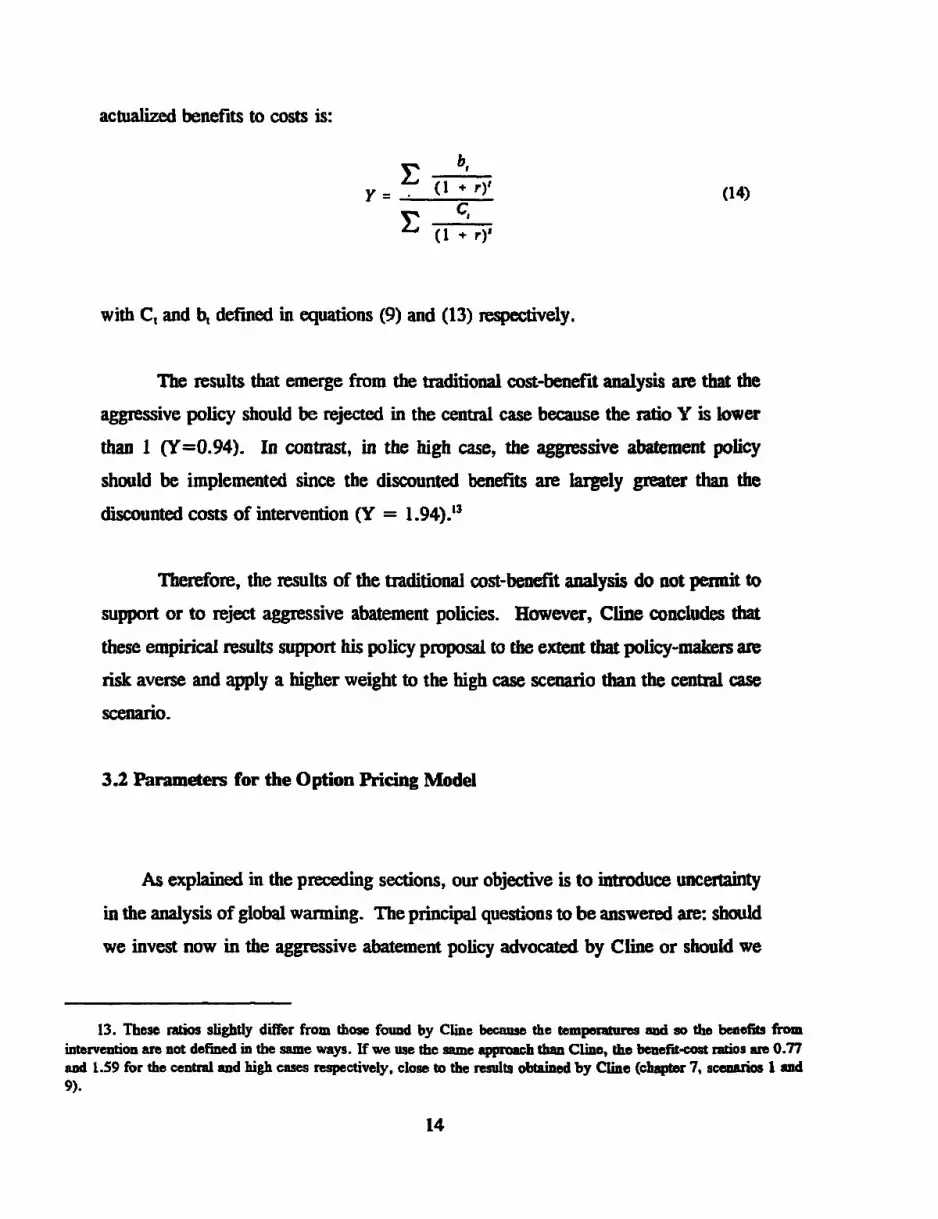
Figure 3 depicts the optimal path of CO2 emission over the period 1990-2275

for different degree of uncertainty.'9 The optimal path is sensitive to the degree of

uncertainty, specifically in the beginning of the period. The optimal path, when the

uncertainty is around 8 percent annually, would cut emissions by 15-20 percent in the

first decades from baseline, rising gradually to 80 percent in the next century.

However, when the uncertainty rises to 10 percent, the CO2 cutback would be only

5-10 percent in the furst decades. These results can be compared with the 40 percent

cutback recommended by Cline in the next few decades, and are close to the level

proposed by Nordhaus and those recommended recently by the European Union.

4 Concluding Remarks

Uncertainty is an inherent phenomena in global warming issues, and thus it

must be explicitly taken into account in the evaluation of policies. Although the major

concern remains the uncertainty around the scientific evidence of climate changes, the

economic analysis provides some guidance whether governments should intervene in

19. The abatement ratio is defined as the CO2 cutback from baseline.

18

the foreseen future.

On the basis of the option-valuation approach, this paper has examined the

impact of uncertainty on the costs-benefits analysis. The major conclusions are the

following:

* The aggressive proposal presented by Cline (1992) appears to be optimal for

a relatively low degree of uncertainty around the costs and benefits of limiting

global warming. This result is valid in the case where the increase in

temperature in the long term is about 18 C° (high case scenario), and the

discount rate is equal to 1.5.

* However, the action should be delayed if the uncertainty is higher than 6

percent per annum. The optimal date of intervention calculated in the paper,

ranging from 35 years to 126 years from now, accounts for the possibility to

accumulate future information and for the increase in irreversible damages

during the waiting period compared to those which would have prevailed if the

action was taken from the start.

* In case of relative high uncertainty, it may be optimal to implement today

a less aggressive policy. If the Cline's proposal is to limit the level of CO2

emission to 4 GtC annually, a ceiling of 5.5-6.5 GtC --about the existing level

in 1990- seems more appropriate for a level of uncertainty ranging around 8-

10 percent annually.

Finally, we would like to conclude that the approach followed in this paper

could be imprved in numerous ways. As discussed earlier, uncertainty around cost

and benefits is assumed to be exogenous and constant over time. It would be certainly

more realistic to consider uncertainty as endogenous, varying, for example, with the

increase in global warming or the magnitude of the policies to limit global carbon

19

emissions. Clearly, additional work is required in this area in buth an analytical and

empirical perspectives.

20

Appendix

In this appendix, the impact of changes in uncertainty on the option value (W) is

discussed in more detail. While an increase in the overall uncertainty on costs and benefits (a)

will unambiguously increase the option value and thus delay the implementation of policies

against global warming, the impact of variations in individual components -uncertainty on

benefits (ri,) or on costs (crO)- remains ambiguous. Below is a detailed description.

A. The Impact of a Change in Overal Uncertainty

Substituting equation (4) into equation (6), the option value can be written as:

W . (Y' - I)F( VyY )r71r - i,

All variables have been defined in the main text. The impact of a change in overall

uncertainty is therefore equal to:

dW dW dY' d7dc9 dY dv dr9

The sign of dW/da2 is unambiguously positive, as demonstrated below:

dY I_ < O

d (--lI)2

dW W [ In 1dY- (Y- -I) (Yi --I) F

dv r - 2 [( FrV) 2 05r - 2F F]rS.[( )( rF V 0.5) *

because as v > 0(aF - av)2

21

B. The Impact of a Change in Individual Components of Uncertainty

The impact of a variation in the uncertainty around benefits and costs on the option

value can be expressed, respectively, as follows:

dW dWdor dWdav da2 dorv do 2( UVV¢)> f

dW- dW aV_ = _~2(arv - OVFOF) > ° if > OVF

a is the vo,atility of Y, which is a ratio of benefits (V) over costs (F).

From these two equations, we can observe that the impact of a change in the

individual uncertainties on the value of the option is ambiguous. For example, the sigr of

the impact of a change in civ on W depends on the values of: (i) the correlation between the

costs and the benefits associated with the policies against global warming; (ii) the uncertainty

on benefits; (iii) the uncertainty on costs. To illustrate, the option value is more lik to be

influenced positively by an increase in the uncertainty on benefits (dW/dav ) if the correlation

between costs and benefits is low and if the uncertainty on benefits is low relative to the

uncertainty on costs.

The numerical exercise simulated in Table 5 of the main text assumes that the

variation in the uncertainty on costs equals that in the uncertainty on benefits (daF = dav )-

In this case, the resulting impact on the option value is unambiguously positive, as

demonstrated below:

dW = -do,+ado,aoF, a°rv

= 2 d ( + c)) ( I - w) do°F > 0

22

Bibliogmphy

Arrow, KJ. and A.C. Fisher (1974), 'Environmental Preservation, Uncertainty and Irreversibility',

Ouaerlv Journal of Economics, 88(2), 312-319.

Ayres, R.U. andJ. Walter(1991), 'ThoGreehouse Effect: Damages, Costsand Abatement', Enviromenta

and Resource Economics, 1(3), 237-270.

Birsail, N. and A. Steer (1993), 'Act Now on Global Warming - But Don't Cook the Books', Finance nd

Develonment, 30.

Cline, W.R. (1992), The Economics of Global Warming, Washington, The Instinte for International

Economy. 399 p.

Cline, W.R (1993), Modeltina Economidaly Efficient Abatement of Greenhoe Gasos, Inst for

Inurnaional Economics. September.

Daily, G.C., P.R. Ehrlich, H.A. Mooney, and AH. EhrLich (1991), 'Greenhouse Econmics: Learning

Before You Leap', Ecolonical Economics, 4(1), 1-10.

Dixit, A. (1992), 'Investment and Hlysteresis', Journal of Economic Persoectives, 6(l), 107-32.

Drepper, F.R. and B.A. Mansson (1993), 'Inter-temporal Valuation in an Unpredictable Environment',

Ecological Economics, 7(1), 43-67.

Fankhawer S. (1992), 'Global Warming Damage Costs: Some Monetuy Estimates", London: Center for

Social and Economic Research on the Global Environment, meo, AugusL

Hanley, N. and C.L Spash (1993), Cost-Benefit Analysis and the Enviromn, Edward Elgar PubL. Hans.

Hoeny, C. (1974), 'Inveatment Decisions Under Uncertainty: the Irreversibility Effect', Anerican Economic

Raviw, 64(6), 1006-1012.

McDonald, R. and D. Siegel (1986), -rhe Value of Waiting to Invest', Ouazterl Jourtal of Economic s,

November, 707-727.

23

Morgocstora, R.D. (1991), 'Towards a Comprehensive Approach to Global Climat Change Mitigation',

American Economic Review, 81(2), 140-145.

Nordhaus, W.D. (1991a), 'To Slow or not to Slow: the Economics of the Greenhouse Effect', ThoEconomic

Journl, 101, 920-937.

Nordhsus, W.D. (1991b), 'A Sketch of the Economics of the Greenhouse Effect', American Economic

Reiow, 81(2), 146-150.

Nordhaus, W.D. (1993), 'Reflections on the Economics of Climate Change', Joural of Economic

Permvectives, 7(4), 11-25.

Pearce, D.W. and A. Markandya (1990), L'Evaluation Mon6taire des Avantans des Politiques de

l'Environnement, OCDE, Paris.

Pindick, R.S. (1991), 'Irreversibility, Uncertainty, and Ivestment', Journal of Economic Liture, 39,

1110-1148.

Reilly, J.M. and K.R. Richards (1993), 'Climate Change Damage and the Trace Gas Inudx Issue',

Environmental and Resource Economics, 3(1), 4142.

Samuelson, P.A. (1965), 'Rational Theory of Warmnt Pricing', Industrial Manaiement Review, 6: 13-31.

Scholling, T. C. (1992), 'Some Economics of Global Warming', American Economic Review, 82(1), 1-14.

Titus J. (1992). "The Cost of Climaen Change to the United States", in S.K. Majumbar et al., eds, Global

Climate Chlie"' Imnlications. Chlennss and Mitimtion Measures.

LJNEP (1991), Climate Cbanze, UNEP, Geneva.

Weisbrod, B.A. (1964), 'Colective-Consumption Services of Individual-Consumption Goods', erk

Joumal of Economics, 68,471477.

World Bank (1991), Decision-MakinaunderUncertintv, Washington, The World Bank, Indury and Energy

Deparment Woring Paper, Energy Series Paper No 39.

24

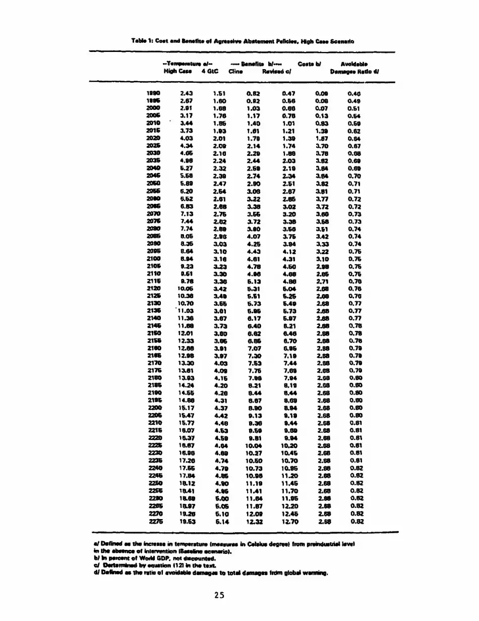
Tabe 1: Cost aud Benefits of Agragalwv Abeatamn PoeIes. Hgh Case Ssneulo

-Tene,atur gi- - BDenefit hi- Coste hi AvolableHioh Case 4 CtC Cline Revised cl Damags Rateo di

1390 2.43 1.61 0.82 0.47 0.00 0.40loSs 2.67 1.60 0.32 0.56 0.08 0.4020oo 2.01 1.08 1.03 0.96 0.07 0.61200Z 3.17 1.76 1.17 0.75 0.13 0.642010 3.44 1.95 1.40 1.01 0.83 0.602015 3.73 1.93 1.61 1.21 1.33 0.822020 4.03 2.01 1.73 1.39 1.87 0.642025 4.34 2.09 2.14 1.74 3.70 0.672030 4.06 2.10 2.29 1.09 3.73 0.052031 4.39 2.24 2.44 2.03 3.92 0.6a2040 5.27 2.32 2.63 2.19 3.84 0.610204 S..8 2.33 2.74 2.34 3.94 0.702050 5.89 2.47 2.30 2.11 3.92 0.71205 6.20 2.-4 3.06 2.67 3.91 0.712060 6.62 2.61 3.22 2.85 3.77 0.722095 6.83 2.99 3.38 3.02 3.72 0.722070 7.13 2.76 3.66 3.20 3.66 0.732075 7.44 2.02 3.72 3.38 3.58 0.732O0 7.74 2.80 3.00 3.S0 3.51 0.74208E 8.05 2.98 4.07 3.75 3.42 0.742090 8.35 3.03 4.26 3.14 3.33 0.742035 8.94 3.10 4.43 4.12 3.22 0.752100 9.94 3.16 4.61 4.31 3.10 0.762105 9.23 3.23 4.78 4.50 2.93 0.752110 0.61 3.30 4.06 4.68 2.35 0.76211S 3.76 3.36 5.13 4.80 2.71 0.782120 10.06 3.42 6.31 5.04 2.00 0.762125 10.36 3.49 6.51 5.25 2.08 0.702130 10.70 3.55 6.73 5.43 2.69 0.77213 ' 11.03 3O. 6.5 L.73 2.63 0.772140 11.38 3.07 6.17 L.07 2.S 0.772145 11.68 3.73 6.40 921 2.9B 0.782160 12.01 3.00 6.62 6.46 2.93 0.79211 12.33 3.06 0.96 6.70 2.68 0.792160 12.66 "I0 7.07 6.96 2.9 0.792165 12.9B 3.97 7.30 7.19 2.98 0.792170 13.30 4.03 7.S3 7.44 2.95 0.792175 13.51 4.09 7.76 7.63 2.08 0.792130 13.33 4.15 7.38 7.34 2.G9 0.502136 14.24 4.20 8.21 8.13 2.69 0.502190 14.56 4.20 B.44 B.44 2.66 0.902139 14.89 4.31 8.67 8.69 2.66 0.302200 1.17 4.37 8.30 9.94 2.69 0.902205 16.47 4.42 9.13 9.19 2.65 0.802210 16.77 4.48 9.38 9." 2.66 0.812215 13.07 4.53 9.09 9.60 2.68 0.812220 1 .37 4.S9 9.31 9.34 2.69 0.91222C 16.87 4.04 10.04 10.20 2.68 0.912230 16.93 4.83 10.27 10.45 2.66 0.912236 17.20 4.74 10.60 10.70 2.68 0.912Z40 17.65 4.79 10.73 10.93 2.69 0.822246 17.84 4.56 10.36 11.20 2.68 0.922250 L912 4.90 11.19 11.45 2.66 O.9222R; 13L41 4.06 11.41 11.70 2.68 0.822230 13.63 5.00 11.64 11.95 2.66 0.93225 18.97 5.06 11.97 12.20 2.96 0.922207 13.L2 5.10 12.09 12.45 2.69 0.822Z27 19.63 6.14 12.32 12.70 2.65 0.92

al Definmd the Incess in temeiture Imeasuws in Celiu degrel from preindustial levelin the abse*ce ef hdrventnn lBmarlne en1na.bi In perent of Wodi CDP. not dinounted.al Det ned bl egumtuo 1121 in the text.di Ddiu as h ratio of evolid dantg to otil dnagfercml global warmng.

25

Table 2: Cost Uncertainty a/In percent of World GDP

Manne-Richels 2.00Edmonds-Barns 0.26Whalley-Wigle 3.52OECD-Green 2.20Cline 0.70

Standard Deviation 1.30Mean 1.74Uncertainty bt 74.71

Source; Cline 119921

Table 3: Benefits Uncertainty cIIn Percent of World GDP

Nordhaus (Al 1.00Cline 1.10Fakhauser 1.30Nordhaus (B) 1.80

Lowest o.ooHighest 5.50

Standard Deviation 1.91Mean 1.78Uncertainty bl 107.30

a/ Based on estimated costs in 2025 and calibratedfor a 40 percent abatement policy from baseline.bI Defined as the ratio of standard deviation to mean.c/ Based on Damages of C02 doubling.dJ Based on a survey of specialists.

26

Table 4:Option-Pricing Approach a/

Central HighCase Case

Benefits volatility b/ 3.80% 3.80%Costs volatility b/ 3.20% 3.20%correlation 5.99% 5.99%Discount rate 1.50% 1.50%Benefits (V) 96.5 198.5Costs (F) 102.3 102.4Benefits growth rate 0.81% 0.69%Costs growth rate 0.16% 0.38%Eff. Benefits growth rate 0.690% 0.8 1%Eff. Costs growth rate 1.34% 1.12%Total volatility 0.23% 0.23%

1.8 2.4

Y* 2.2 1.7Y =(V/F) 0.9 1.9W c/ 494.0 1313.0ElT), in years d/ 133.6 -36.9

All variables are defined in the text

a/ In percent of World GDP, otherwise specified.b/As determined in Tables 2 and 3cl In trillions of 1990 US dollars.dl Optimal timing determined by equation (81 in the text.

27

Table 5:High Case: Sensitivity Analysis al

Changes in Total Effective Volatility

Benefits volatility 0.00%. 2.00% 4.00% 6.00% 8.00% 10.00% 12.00%Costs volatility 0.00% 2.00% 4.00% 6.00% 8.00% 10.00% 12.00%Correlation 5.99% 5.99% 5.99% 5.99% 5.99% 5.99% 5.99%Discount rate 1.50% 1.50% 1.50% 1.50% 1.50% 1.50% 1.50%Benefits (V) 198.5 198.5 198.5 198.5 198.5 198.5 198.5Costs (F) 102.4 102.4 102.4 102.4 102.4 102.4 102.4Benefits growth rate 0.69% 0.69% 0.69% 0.69% 0.69% 0.69% 0.69%Costs growth rate 0.38% 0.38% 0.38% 0.38% 0.38% 0.38% 0.38%Eff. Benefits growth rate 0.81% 0.81 % 0.81% 0.81 % 0.81% 0.81% 0.81%Et. Costs growth rate 1.12% 1.12% 1.12% 1.12% 1.12% 1.12% 1.12%Total volatility 0.00% 0.08% 0.30% 0.68% 1.20% 1.88% 2.71 %x na 2.9 2.2 1.9 1.6 1.5 1.4

vo 1.4 1.5 1.8 2.2 2.6 3.1 3.7Y =(VIF) 1.9 1.9 1.9 1.9 1.9 1.9 1.9W na 1252.1 1365.6 1715.1 2267.2 3044.6 4093.4

Optimal TimingEM, in years b/ 0 0 0 35.8 94.5 151.8 207.2E(T). in years cJ - - - 35.0 72.0 115.0 126.0Optimal PolicyC02 Ceilings dl 2.4 3.5 4.8 5.7 6.4 7.0

a/ In percent of World GDP. otherwise specifiedbl Optimal timing is determined by equation (8) which assumes that the level of irreversibledamages would remain the same than if the action was taken 1rom the start.cl Optimal timing accounting for the increase over the waiting period of the irreversible damages.di Optimal C02 ceiling to be implemented from 1990 to 2275

28

Percent of Waild GOP

Percent of GOP o - Ca W l a mn C ( a

° P S P P ° P P oP 95 0@@ '0 -. N III ~~~ C CD 1995 *

1995 , * , | , | , ~ | 2005

2005 \ 2015

2005 2025

2025 2035

2035 2045

20495 * | 2055

2055 -. g 2055

2065 S27

2075 2085S

2095 o 2095

2105 21052115 2115

214S a 6 2125 ft2125 - 8 2135 tg 2135

2145S 2145 CS,

2155 3 2155

2165 | 2165

2175 "Al 2175

2155 2

2195 2195

2205 22215 * ~~~~~~~~~~~~~~~~205

2225 2215

2235 2225

2245 5 2235

2255 - 2245

2265 2255

2275 2255

2275

Igue 34 O7ptinl RaI tae o;f

o.g 1~~~~~~~~~~~~Outo

0.8

0.7

0.6 NIS

AAA a**S

*

A'

0.3 ~ ~ 3

Policy Research Working Paper Series

ContactTitle Author Date for paper

WPS1397 Are Private Capital Flows to Ur Dadush December 1994 J. OueenDeveloping Countries Sustainable? Ashok Dhareshwar 33740

Ron Johannes

WPS1398 The Cost of Air Pollution Abaternent Raymond S. Hartman December 1994 E. SchaperDavid Wheeler 33457Manjula Singh

WPS1399 How Important to India's Poor is the Martin Ravallion December1994 P. CookUrban-Rural Composition of Growth? Gaurav Dan 33902

WPS1400 Technical and Marketing Support Brian Levy with December 1994 D. EvansSystems for Successful Small and Albert Berry, Motoshige Itoh, 38526Medium-Size Enterprises in Four Unsu Kim, Jeffrey Nugent,Countries and Shujiro Urata

WPS1401 Colombia's Small and Medium-Size Albert Berry December 1994 D. EvansExporters and Their Support Systems Jose Escandon 38526

WPS1402 Indonesia's Small and Medium-Size Albert Berry December1994 D. EvansExporters and Their Support Systems Brian Levy 38526

WPS1403 Small and Medium-Size Enterprise Motoshige Itoh December 1994 D. EvansSupport Policies in Japan Shujiro Urata 38526

WPSI1404 The Republic of Korea's Small and Unsu Kim December 1994 D. EvansMedium-Size Enterprises and Their Jeffrey B. Nugent 38526Support Systems

WPS1405 Growth and Poverty in Rural India Martin Ravallion January 1995 WDRGaurav Datt 31393

WPS1406 Structural Breaks and Long-Run Javier Le6n January 1995 R. LuzTrends in Commodity Prices Raimundo Soto 31320

WPS1407 Pakistan's Agriculture Sector. Rashid Faruqee January 1995 F. WillieIs 3 to 4 Percent Annual Growth 82262Sustainable?

WPS1408 Macroeconomic Management and Jun Ma January 1995 C. JonesIntergovemmental Relations in 37754China

WPS1409 Restructuring Uganda7s Debt Kapil Kapoor January 1995 E. SpanoThe Commercial Debt Buy-Back 35538Operation

WPS1410 Macroeconomic Effects of Temis- Nikola Spatafora January 1995 J. Queenof-Trade Shocks: The Case of Oil- Andrew Warner 33740Exporting Countries

Policy Research Working Paper Series

ContactTitle Author Date for paper

WPS1411 Income Inequality, Welfare, and Nanak Kakwani January 1995 G. EvansPoveny: An Illustralion Using 85783Ukrainian Data

WPS1412 Foreign Technology Imports and XGaomingZhang January 1995 C. JonesEconomic Growth in Devebping Heng-fu ZDu 37754Countries

WPS1413 Endogenous Distortions in Product Marlin Rama January 1995 S. Fallonand Labor Markets Guido Tabellini 38009

WPS1414 The Wold Bank and Legal Technical The Worid Bank January 1995 K MathemovaAss_tance: Initial Lessons Legaj Departe 82782

WPS1415 China's GDP in U.S. Dollars Based Ren Ruoen January 1995 E. aRiRlly-Campbellon Purchasing Power Parity Chen KaW 33707

WPS1416 Informal Regulation of Industrial SheoR Pargal February 1995 E. SchaperPollution in Developing Counties: David Wheeler 33457Evidence from Indonesia

WPS1417 Uncertainty and Global Warming: An Andrea Baranzini February 1995 C. DellOption-Pricing Approach to Policy Marc Chesney 85148

Jacques Morisset