Uniformity constant estimates for some elementary domains

Helsinki Analysis Seminar, 10.3.2003

Uniformity constant estimates forsome elementary domains

Henri LindenUniversity of Helsinki,

Department of Mathematics,PL 4, Yliopistonkatu 5,00014 Helsinki, Finland

E-mail: [email protected]

AbstractIt is well-known that e.g. quasidisks are uniform domains,

but finding the sharp constants is probably an open questionfor most domains. Here the question of the best constant isstudied for some simple domains, in particular for the angulardomains.

– Typeset by FoilTEX – 1

Preliminaries

Uniform domains were introduced by O. Martio and J. Sarvas in[MS]. A domain G ⊂ Rn is said to be uniform if there exists aconstant c ≥ 1 such that all z1, z2 ∈ G can be joined by an arcα ⊂ G where

i) l(α) ≤ c|z1 − z2|,ii) min

j=1,2l(αj) ≤ cdist(z, ∂G)

for each z ∈ α, where α1, α2 are the components of α \ {z}.

In this work we shall consider another definition of uniform domains,originally stated by F. Gehring and B. Osgood in [GO] The alternativedefinition (see 1.3) is interesting because it gives a direct comparisonbetween the quasihyperbolic metric and the so-called j-metric.


Quasihyperbolic and j-metric

For a given domain G ⊂ Rn we may define the quasihyperbolicdistance between x and y in G by

kG(x, y) = infα∈Γxy

∫α

|dx|d(x)

, (1.1)

where d(x) denotes the distance to the boundary, dist(x, ∂G), andΓxy stands for all rectifiable curves joining x and y in G. It is clearthat kG is a metric on G. Moreover, kG has the following monotoneproperty: if G and G′ are domains with G′ ⊂ G and x, y ∈ G′, thenkG′(x, y) ≥ kG(x, y). We also define

jG(x, y) = log(1 +

|x− y|min{d(x), d(y)}

)(1.2)

for every x, y ∈ G. This is also a metric, often referred to as the j-metric. It is known to have properties similar to the quasihyperbolicmetric. For instance, both metrics are invariant under translations,strechings and orthogonal mappings.


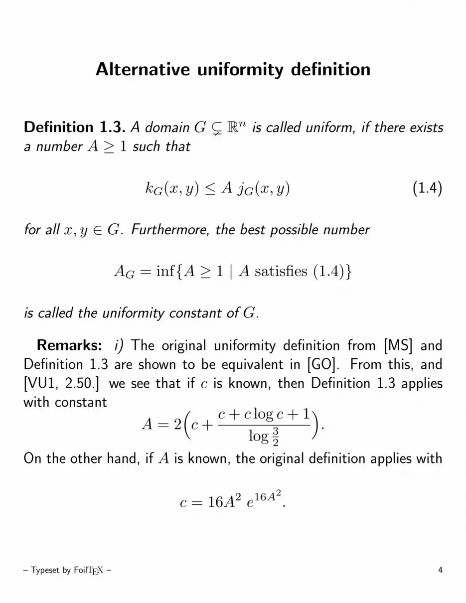
Alternative uniformity definition

Definition 1.3. A domain G ( Rn is called uniform, if there existsa number A ≥ 1 such that

kG(x, y) ≤ A jG(x, y) (1.4)

for all x, y ∈ G. Furthermore, the best possible number

AG = inf{A ≥ 1 | A satisfies (1.4)}

is called the uniformity constant of G.

Remarks: i) The original uniformity definition from [MS] andDefinition 1.3 are shown to be equivalent in [GO]. From this, and[VU1, 2.50.] we see that if c is known, then Definition 1.3 applieswith constant

A = 2(c +

c + c log c + 1log 3

2

).

On the other hand, if A is known, the original definition applies with

c = 16A2 e16A2.


Remarks

ii) The difficulties in computing the uniformity constant is mostoften connected to the fact that the quasihyperbolic metric fails tohave a nice explicit expression for most domains, and usually thequasihyperbolic geodesics are unknown. In the general case someregularity properties have been proven, though, by G. Martin in [MA].

iii) The explicit uniformity constant is known only in the cases ofthe disk Bn and the halfspace Hn, and its value is then 2, which isshown in [VU2, Lemma 2.41] for Hn and in [AVV, Lemma 7.56] forBn.


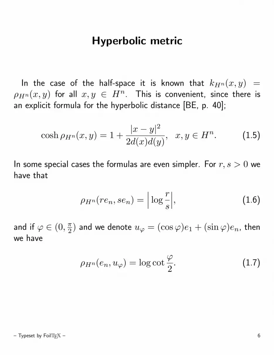
Hyperbolic metric

In the case of the half-space it is known that kHn(x, y) =ρHn(x, y) for all x, y ∈ Hn. This is convenient, since there isan explicit formula for the hyperbolic distance [BE, p. 40];

cosh ρHn(x, y) = 1 +|x− y|2

2d(x)d(y), x, y ∈ Hn. (1.5)

In some special cases the formulas are even simpler. For r, s > 0 wehave that

ρHn(ren, sen) =∣∣∣ log

r

s

∣∣∣, (1.6)

and if ϕ ∈ (0, π2) and we denote uϕ = (cos ϕ)e1 + (sinϕ)en, then

we have

ρHn(en, uϕ) = log cotϕ

2. (1.7)


Inequalities

In the ball Bn we only get inequality kBn(x, y) ≤ ρBn(x, y), butthis is also often helpful. Here we have the formula [BE, p. 35]

sinh2(12ρBn(x, y)

)=

|x− y|2

(1− |x|2)(1− |y|2). (1.8)

For 0 < t < 1 we have that

ρBn(0, te1) = log1 + t

1− t= 2ar tanh t. (1.9)

For future use we also mention some useful inequalities, such asthe relations for the hyperbolic functions

log(1 + x) ≤ ar sinhx ≤ 2 log(1 + x), x ≥ 0 (1.10)

2 log(1 +

√12(x− 1)

)≤ ar coshx ≤ 2 log

(1 +

√2(x− 1)

), x ≥ 1,(1.11)

and Bernoulli’s inequalities

log(1 + as) ≤ a log(1 + s); a ≥ 1, s ≥ 0 (1.12)

a log(1 + s) ≤ log(1 + as) : a ≤ 1, s ≥ 0. (1.13)


Geodesics in Rn \ {0}

In the case of Rn\{0} Martin and Osgood (see [MO]) have deter-mined the geodesics. Their result states that given x, y ∈ Rn\{0},the geodesic segment can be obtained as follows; Let ϕ be the anglebetween the segments [0, x] and [0, y], 0 < ϕ < π. The triple0, x, y clearly determines a 2-dimensional plane Σ, and the geodesicsegment connecting x to y is the logarithmic spiral in Σ with polarequation

r(ω) = |x| exp(ω

ϕlog

|y||x|

).

In the sequel we denote Rn∗ = Rn \ {0}. Then we can prove the

following lemma using the above representation for the geodesic.Lemma 2.1. In the domain Rn

∗ = Rn \ {0} the quasihyperbolicdistance is given by the formula

kRn∗ (x, y) =

√ϕ2 + log2 |x|

|y|,

where ϕ denotes the angle between [0, x] and [0, y].


Previous results

Using Lemma 2.1 one can show that

kRn∗ (x, y)2 = ϕ2 + log2 |x|

|y|≤(cjRn

∗ (x, y))2 +

(jRn

∗ (x, y))2

= (1 + c2)jRn∗ (x, y),

if one can show that ϕ ≤ cjRn∗ (x, y). Vuorinen shows in [VU2] that

we can obtainϕ ≤ π

log 2jRn

∗ (x, y),

and has later shown, by using l’Hospital’s monotone rule (cf. [AVV,Theorem 1.25]) that

ϕ ≤ π

log 3jRn

∗ (x, y).


Uniformity constant of Rn∗

Theorem 2.2. For the domain Rn∗ = Rn \ {0} the uniformity con-

stant isARn

∗ =π

log 3≈ 2.8596.

Sketch of proof: We begin with noticing that by the results ofMartin and Osgood it is essentially enough to prove the problem forR2 \ {0}. Moreover, since for any point x ∈ Rn

∗

jRn∗ (x,−x) = log 3 and kRn

∗ (x,−x) = π,

it is immediate that the constant π/ log 3 is attained, and what wein fact need to do is to prove the inequality (1.4) of the uniformitydefinition.

Assume that x, y ∈ R2 \ {0} and that |x| ≤ |y|. Using thedefinition of the metric jRn

∗ we obtain

jRn∗ (x, y) = log

(1 +

√|x|2 − 2x · y + |y|2

|x|

).


By Pythagoras’s theorem

ϕ = arc cos(|x|2 + |y|2 − |x− y|2

2|x||y|

).

Using Lemma 2.1, we see that in order to satisfy (1.4), the numberc must in fact satisfy the inequality

arc cos2(|x|2 + |y|2 − |x− y|2

2|x||y|

)+ log2 |x|

|y|

≤ c2 log2(1 +

√|x|2 − 2x · y + |y|2

|x|

).

By the invariance of jRn∗ and kRn

∗ with respect to stretchings andorthogonal mappings, we may now assume that x = e1 and y = teiθ,where t ≥ 1 and 0 ≤ θ ≤ π. Clearly the goal is then to find themaximum of the expression

arc cos2(|x|2+|y|2−|x−y|2

2|x||y|

)+ log2 |x|

|y|

log2(1 +

√|x|2−2x·y+|y|2

|x|

) . (2.3)


This reduces to a function of t and θ;

F (θ, t) =θ2 + log2 t

log2(1 +√

1 + t2 − 2t cos θ), (2.4)

where t ≥ 1 and 0 ≤ θ ≤ π.

This can be shown to be increasing with respect to θ and decreasingwith respect to t, and thus the maximum of the function F (θ, t), isattained at F (π, 1). Then c = π/ log 3.


The angular domain Sϕ

Next we consider the angular domain

Sϕ = {(r, θ) ∈ R2 : 0 < θ < ϕ}.

It is easy to obtain a lower bound for the uniformity constant; De-noting the bisector of the angle by `ϕ, the following theorem is easyto obtain for x, y ∈ `ϕ.Lemma 3.1. For the domain Sϕ and points x, y ∈ `ϕ

kSϕ(x, y) =1

sin ϕ2

jSϕ(x, y).

Proof: By similarity invariance, we may assume that |y| ≥ |x| = 1,and we then see that

kSϕ(x, y) =∫

[x,y]

|dt|d(t)

=∫

[x,y]

|dt||t| sin ϕ

2

=

∣∣∣∣∣∫ |y|

1

dt

t sin ϕ2

∣∣∣∣∣ = 1sin ϕ

2

log |y|. (3.2)


Lower bound of ASϕ

It is also easy to explicitely calculate

jSϕ(x, y) = log(1 +

|y| − 11

)= log |y|, (3.3)

Thus we see that the number 1/ sin(ϕ/2) is in fact a lower boundfor the uniformity constant. The number 2 is easily seen to be at-tained for every angle. Thus we can establish a lower bound

ASϕ ≥ max{

2,1

sin ϕ2

}(3.4)

for the domain Sϕ.


Upper bound of ASϕ

Lemma 3.5. For any x, y ∈ Sϕ,

kSϕ(x, y) ≤ (4 +1

sin(ϕ/2))jSϕ(x, y).

Proof: Let x, y ∈ Sϕ be arbitrary, and choose points x′, y′ ∈ `ϕ

such that [x, x′] and [y, y′] are orthogonal to `ϕ. By the triangleinequality we have that

kSϕ(x, y) ≤ kSϕ(x, x′) + kSϕ(x′, y′) + kSϕ(y′, y).

As seen, the middle term allows an estimate

kSϕ(x′, y′) ≤ 1sin ϕ

2

jSϕ(x′, y′).

We now show that jSϕ(x′, y′) ≤ jSϕ(x, y). This is true exactlywhen

|x− y|min{d(x), d(y)}

≥ |x′ − y′|min{d(x′), d(y′)}

,


Obviously min{d(x), d(y)} ≤ min{d(x′), d(y′)}, and it is alsoclear that |x′ − y′| ≤ |x− y|. Thus

kSϕ(x′, y′) ≤ 1sin ϕ

2

jSϕ(x, y).

After this we concentrate on the remaing terms, i.e. we want toshow that there are constants cx, cy ≥ 1 such that

kSϕ(x, x′) ≤ cxjSϕ(x, y), (3.6)

kSϕ(y, y′) ≤ cyjSϕ(x, y). (3.7)

For this we may, without loss of generality, assume that d(x) ≤ d(y),and also that both

y 6∈ B(x, |x− x′|) ∩ Sϕ,

x 6∈ B(y, |y − y′|) ∩ Sϕ

hold. Namely, if not, there would exist a hyperbolic H2-geodesicconnecting the points x and y, and we would have kSϕ(x, y) ≤2jSϕ(x, y).


Now, by the choice of the points x′ and y′ it is obvious that thereexists a hyperbolic geodesic connecting x and x′, and one connectingy and y′. Thus we see that

kSϕ(x, x′) ≤ 2jSϕ(x, x′),

kSϕ(y, y′) ≤ 2jSϕ(y, y′).It now remains to show that jSϕ(x, x′) ≤ cxjSϕ(x, y) andjSϕ(y, y′) ≤ cyjSϕ(x, y) for some constants cx, cy ≥ 1. Since byassumption d(x) ≤ d(y), and also d(x) ≤ d(x′), the first inequalityfollows with cx = 1 from the inequality

|x− x′|d(x)

≤ |x− y|d(x)

,

which is certainly true, since we have assumed that |x−x′| ≤ |x−y|.The second inequality follows with cy = 1 from the inequality

|y − y′|d(y)

≤ |x− y|d(x)

,

which holds since we have assumed that |y−y′| ≤ |x−y|, and thatd(x) ≤ d(y). Hence, in (3.6) and (3.7) we may choose cx = cy = 2.


Then we may derive an upper bound for the uniformity constantby seeing that

kSϕ(x, y) ≤ kSϕ(x, x′) + kSϕ(x′, y′) + kSϕ(y′, y)

≤ 2 jSϕ(x, x′) +1

sin(ϕ/2)jSϕ(x, y) + 2 jSϕ(y′, y)

≤ 2 jSϕ(x, y) +1

sin(ϕ/2)jSϕ(x, y) + 2 jSϕ(x, y)

= (4 +1

sin(ϕ/2))jSϕ(x, y).


Special cases

Lemma 3.8. In the domains Sϕ, unregarded of ϕ, the following hold:

i) If arg(x) = arg(y) = θ, then

kSϕ(x, y) ≤ 1min{sin θ, sin(ϕ− θ)})

jSϕ(x, y).

ii) If |x| = |y|, then

kSϕ(x, y) ≤ 2jSϕ(x, y).

Proof: i) Without loss of generality we may assume that θ < ϕ/2.Then clearly

S2θ ={(r, θ) ∈ R2 : 0 < ω < 2θ

}⊂

{(r, θ) ∈ R2 : 0 < ω < ϕ

}= Sϕ.

Then by the monotonicity property of k we have that kSϕ(x, y) ≤kS2θ

, but clearly jSϕ(x, y) = jS2θ(x, y).


Since x and y are contained in the bisector of the domain S2θ,arguing as in (3.2) and (3.3) shows that

kSϕ(x, y)jSϕ(x, y)

≤kS2θ

(x, y)jS2θ

(x, y)≤ 1

sin θ.

ii) Clearly the case where x and y are on the same side of `ϕ

is trivial. Thus we assume that arg(x) < ϕ/2 < arg(y), that|x| = |y| = 1 and that in fact arg(x) = ϕ− arg(y) = θ. Namely,if not, we can use the monotonicity property as in the proof of i).Denoting {z} = `ϕ ∩ Sn−1, we see that kSϕ(x, z) = kSϕ(z, y),and using the equality kHn = ρHn and (1.7) we get

kSϕ(x, y) ≤ 2kSϕ(x, z) ≤ 2 logtan ϕ

4

tan θ2

.

By the definition of the j-metric (1.2) and Bernoulli’s inequality(1.12) it then suffices to show that

tan ϕ4

tan θ2

≤ 1 + 2sin(ϕ

2 − θ)sin θ

.

This can be done by elementary analysis.


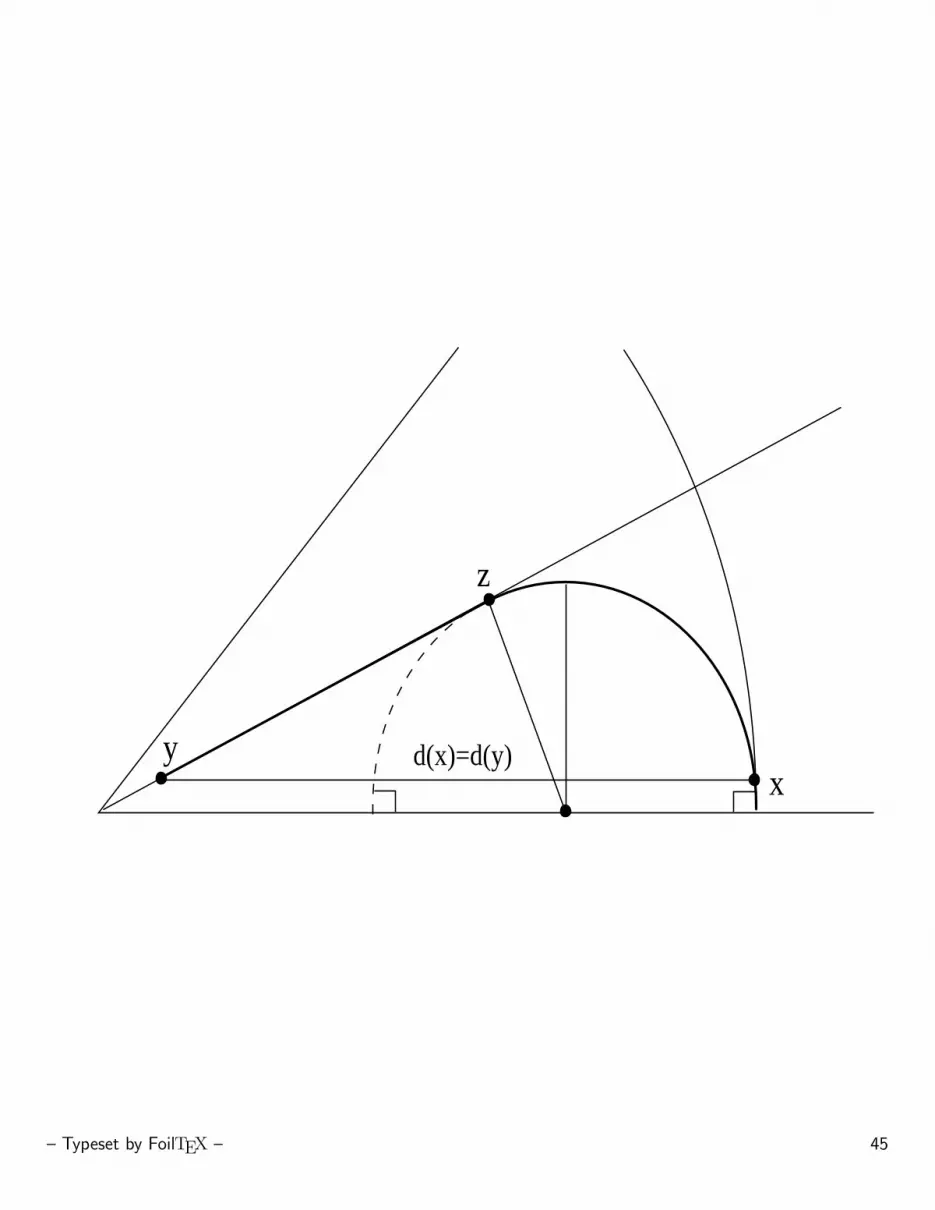
Extremal case

Lemma 3.9. Given points x, y ∈ Sϕ, there is an angle ω ∈ (ϕ, π)and points x′, y′ ∈ Sω such that x′ ∈ `ω, |pr y′| = 1, d(x′) =d(y′) and


≤ kSω(x′, y′)jSω(x′, y′)

.

Here pr y′ denotes the projection of y′ onto ∂Sω.

Figure 1

Lemma 3.10. For the angular domain Sϕ

ASϕ ≤ limx→0y→e1


.

Proof: First, the existence of the limit is guaranteed by Lemma3.5. Denote by Eϕ ⊂ Sω × Sω the set

Eω = {(x, y) : y ∈ `ω/2, |prx| = 1, d(x) = d(y)}.

Recall that ASϕ is defined by

ASϕ = sup{kSϕ(x, y)

jSϕ(x, y): x, y ∈ Sϕ, x 6= y

}.


Let x, y ∈ Sϕ be given. Then by Lemma 3.9 there is some angleϕ ≤ ω < π and a point (x′, y′) ∈ Eω such that


≤ kSω(x′, y′)jSω(x′, y′)

.

We now want to find an upper bound for the ratio k/j of points inEω. Denote by (xt, yt) the point of Eω such that d(x) = d(y) = t.We then want to estimate the function

Φ(t) =kSω(xt, yt)jSω(xt, yt)

.

As can be calculated using elementary geometry (see Figure 2), Φis a function

Φ:(0, tan

ω

2]→ R,

but we are only interested in the restriction of Φ to the interval(0, 1

2 tan(ω/2)

), where the number 1

2 tan(ω/2) is the height of the

isosceles triangle ∆ which has a side orthogonal to the hypotenuseof


the big triangle. Namely, above this line Φ(t) ≤ 2 since the hyper-bolic geodesic is contained in the big triangle. Thus the maximummust be found below this line.

Now, taking the supremum over all points x, y ∈ Sϕ, we note thatfor a fixed ϕ the angle ω given by Lemma 3.9 can be any numberin [ϕ, π). As ω approaches π we see that 1

2 tan(ω/2) → 0. Thus the

limiting case is given by limt→0 Φ(t). The claim follows.


Geometrical lemma

Lemma 3.11. For every point x = (r, θ) ∈ Sϕ there exists exactlytwo circular arcs Cm(x) and CM(x) which are orthogonal to theboundary ∂Sϕ and tangential to the bisector `ϕ/2. In polar coordi-nates these circles are described by

Cm(x) = S1(xm, |xm| sinϕ

2) and

CM(x) = S1(xM , |xM | sinϕ

2),

where

xm =

(r

cos θ −√

cos2 θ − cos2 ϕ2

cos2 ϕ2

, φm

),

xM =

(r

cos θ +√

cos2 θ − cos2 ϕ2

cos2 ϕ2

, φM

)and φm = φM equals 0 or ϕ depending on which component ofSϕ \ `ϕ/2 the point x is contained in.

Figure 3


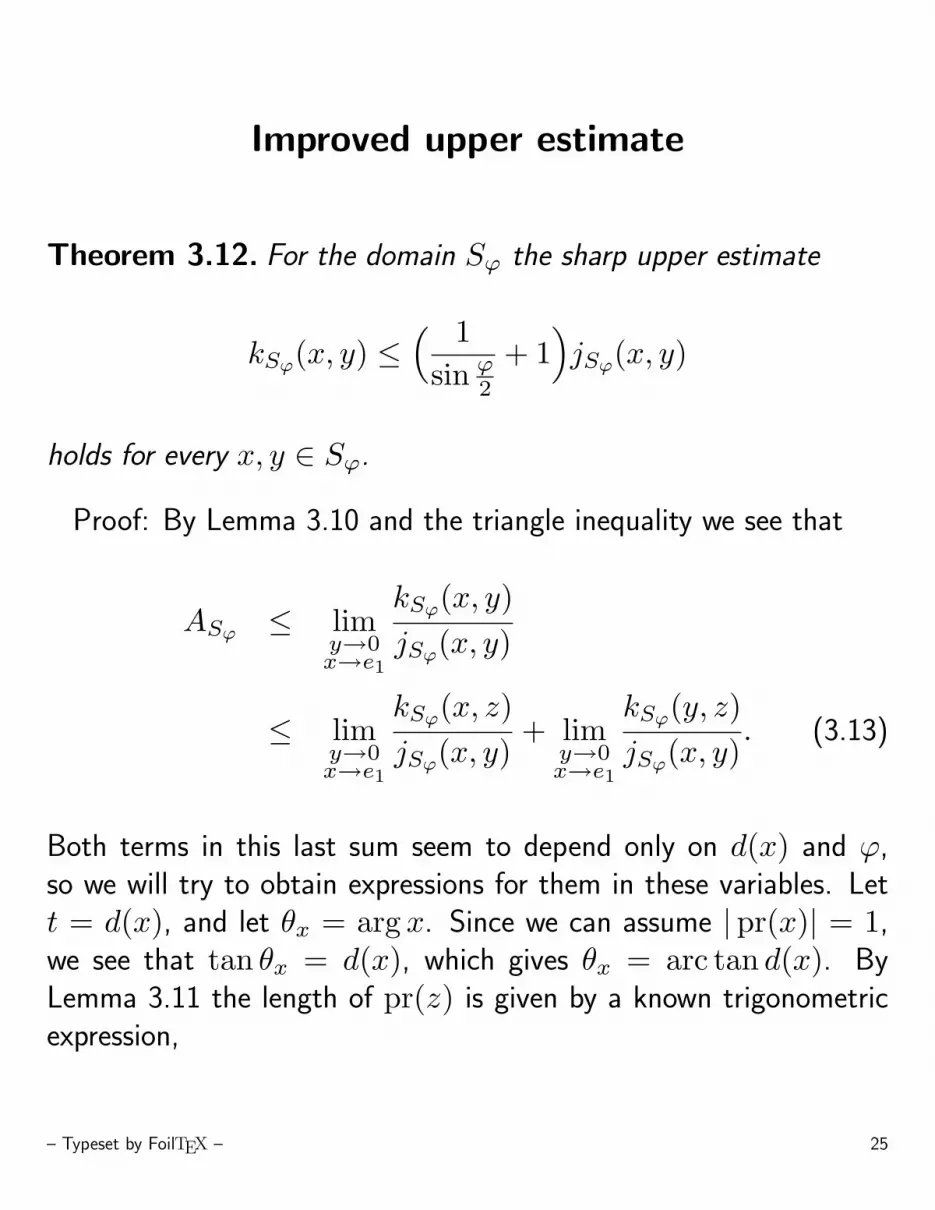
Improved upper estimate

Theorem 3.12. For the domain Sϕ the sharp upper estimate

kSϕ(x, y) ≤( 1sin ϕ

2

+ 1)jSϕ(x, y)

holds for every x, y ∈ Sϕ.

Proof: By Lemma 3.10 and the triangle inequality we see that

ASϕ ≤ limy→0x→e1


≤ limy→0x→e1

kSϕ(x, z)jSϕ(x, y)

+ limy→0x→e1

kSϕ(y, z)jSϕ(x, y)

. (3.13)

Both terms in this last sum seem to depend only on d(x) and ϕ,so we will try to obtain expressions for them in these variables. Lett = d(x), and let θx = arg x. Since we can assume |pr(x)| = 1,we see that tan θx = d(x), which gives θx = arc tan d(x). ByLemma 3.11 the length of pr(z) is given by a known trigonometricexpression,


which gives us

|y − z| =√

1 + t2

(cos θx −

√cos2 θx − cos2 ϕ

2

cos2 ϕ2

)cos

ϕ

2.

We now put

a(t, ϕ) =|y − z|√1 + t2

=

1√1+t2

−√

11+t2

− cos2 ϕ2

cos ϕ2

, (3.14)

where the latter equality is derived from the fact that θx = arc tan t.Now it is easily seen that

j(x, y) = log(1 +

1− t cot ϕ2

t

).

and that

k(y, z) =1

sin ϕ2

log|z||y|

=1

sin ϕ2

log(a(t, ϕ)

√1 + t2 sin ϕ

2

t

)=

1sin ϕ

2

log

[tan ϕ

2

t

(1−

√1− (1 + t2) cos2

ϕ

2

)].


Applying l’Hospital’s rule to the ratio

sinϕ

2k(y, z)j(x, y)

=

log

[tan ϕ

2t

(1−

√1− (1 + t2) cos2 ϕ

2

)]log(1 + 1−t cot ϕ

2t

)and letting t → 0 shows that

sinϕ

2k(y, z)j(x, y)

→ 1. (3.15)

The estimate of the other term is obtained in quite a similar way.First, by (1.5) and using the inequality (1.11) we see that

k(x, z) = ar cosh(1 +

|x− z|2

2d(x)d(z)

)≤ 2 log

(1 +

|x− z|√d(x)d(z)

).

Then we apply the estimate |x−z| ≤ 2a(t, ϕ) tan ϕ2 sin ϕ+π

4 , whichfollows from the fact that the triangle with [x, z] as base and thecenter of Cm(x) as top is isosceles. This gives us the inequality

k(x, z) ≤ 2 log

(1 +

2 a(t, ϕ) tan ϕ2 sin ϕ+π

4√t a(t, ϕ) sin ϕ

2

).


Now we use the same method as previously, that is, we applyl’Hospital’s rule to the ratio

12

k(x, z)j(x, y)

≤log

(1 + 2 a(t,ϕ) tan ϕ

2 sin ϕ+π4√

t a(t,ϕ) sin ϕ2

)log(1 + 1−t cot ϕ

2t

) ,

and let t → 0. This yields

12

k(x, z)j(x, y)

→ 12. (3.16)

Finally, combining (3.13),(3.15) and (3.16) we get

ASϕ ≤ limx→0y→e1

kSϕ(x, z)jSϕ(x, y)

+ limx→0y→e1

kSϕ(y, z)jSϕ(x, y)

=1

sin ϕ2

+ 1.

as stated.


The ϕ-cone Cϕ

After having taken care of the case n = 2 we now turn our interesttowards the general case, i.e. the ϕ-cone

Cn(ϕ) = {z ∈ Rn : z · en = |z| cos ϕ}.

The idea is simply to reduce the problem to the case n = 2. Actually,we get the same constant 1/ sin(ϕ/2) + 1 unregarded of dimensionn.Corollary 3.17. For the domain Cn(ϕ), n ≥ 3, the estimate

kCn(ϕ)(x, y) ≤ AjCn(ϕ)(x, y)

holds for every x, y ∈ Cn(ϕ), if (1.4) holds with constant A in thedomain C2(ϕ) = Sϕ.


The punctured ball Bn \ {0}

For this case a lower bound is immediately given by the constantπ/ log 3, since choosing x = e1/2, y = −e1/2 gives exactly themaximal constant from the case Rn \ {0}. It is also clear that ifboth points x and y are located within the ball Bn(1

2), the situationis reduced to the case Rn \ {0}.

Lemma 4.1. For each point x ∈ B2 \ B2(12) there is a unique

circle Cx such that x lies on this circle, and Cx is tangent to B2(12)

and orthogonal to S1. Denoting {w} = Cx ∩ B2(12), the angle ϕ

between the segments [0, x] and [0, w] is given by the expression

ϕ = arc cos(25|x|2 + 1|x|

)and the center point of Cx is

(|x|2

+1

2|x|,

14|x|

√(4− |x|2)(4|x|2 − 1)

).

Figure 4


The upper bound

Theorem 4.2. For the domain Bn∗ = Bn \ {0} the inequality

2.8596 ≈ π

log 3≤ ABn

∗ ≤ c ≈ 2.8854

applies.

Proof: First of all we remark that it is enough to consider the casen = 2 since for any x, y we may restrict to (Bn \ {0}) ∩ Σ, whereΣ is the 2-dimensional plane determined by 0, x and y.

Assume first that |x| ≤ 12 ≤ |y|. Applying a suitable rotation we

may naturally assume that y = te1 for some t ∈ [12, 1). Without lossof generality we may also assume that the point x lies in the upperhalf plane. Denote also s = |x|, and let ω be the angle between[0, x] and [0, y], as B1 denotes the ball B2(e1

2 , 12). The idea is now

to estimate the geodesic by the circular arc connecting x with e12

and the geodesic Jρ[e12 , y] with respect to the ball B1. Clearly this

is possible, by using the inequality kBn(x, y) ≤ ρBn(x, y), where ρstands for the hyperbolic distance. Denoting z = e1

2 we then obtain

kB2∗(x, y) ≤ kB2

∗(x, z) + kB2

∗(z, y)

≤ kR2∗(x, z) + kB1(z, y) ≤ kR2

∗(x, z) + ρB1(z, y).


Then we may, using Lemma 2.1 and (1.9) define a functionΦ(ω, s, t) according with

Φ(ω, s, t) =kR2

∗(x, z) + ρB1(z, y)

jB2∗(x, y)

=

√ω2 + log2 2s + log 1+2t

1−2t

log(1 +

√s2+(t+1

2)2−2s(t+1

2) cos ω

min{s,12−t}

),

where t and s take values in [0, 1/2). The extremal situation for thissubcase in then obtained by maximizing the function Φ.

Next, assume that 12 ≤ |y| ≤ |x|. Then it is clear that the k-

geodesic Jk[x, y] is contained in the annulus B2 \ B2(12). Thus we

may assume that in fact |x| = |y|, namely, if for instance we haved(x) < d(y), we can rotate the segment [x, y] about the point xsuch that d(x) = d(y), that is |x| = |y|. This operation clearlypreserves the j-distance, and increases the k-distance. Denote theangle between [0, x] and [0, y] by ω, and let |x| = |y| = t. FromLemma 4.1 we get unique points x′ and y′ at S1(1

2) such that theparts of Cx and Cy connecting x with x′ and y with y′, respectively,are the hyperbolic geodesics Jρ[x, x′] and Jρ[y, y′].


The angle between x and x′ is the same as the angle between yand y′, and is given directly by

ϕ = arc cos(25t2 + 1

t

).

Moreover,

kB2∗(x′, y′) = kR2

∗(x′, y′) = ω − 2 arc cos

(25t2 + 1

t

).

It is also easy to calculate the hyperbolic distance ρB(x, x′) =ρBn(y, y′) explicitely using (1.8). It is given by

ρBn(x, x′) = 2 ar sinh( 1√

5

√4t2 − 11− t2

).

Then, defining a function Ψ(ω, t) by

Ψ(ω, t) =ρB2(x, x′) + kR2

∗(x, y) + ρB2(y, y′)

jB2(x, y)

=4 ar sinh

(1√5

√4t2−11−t2

)+(ω − 2 arc cos

(25

t2+1t

))log(1 + 2t sin(ω

2 )

1−t

) ,


the extremal situation for this subcase in obtained by maximizingthe function Ψ.

Denoting

P = sup{Φ : 0 ≤ ω ≤ π, 0 ≤ t < 1/2, 0 < s ≤ 1/2} and

Q = sup{Ψ : 0 ≤ ω ≤ π, 1/2 ≤ t < 1}.it is clear that

AB2∗≤ max

{P,Q,

π

log 3

}.

Note, though, that in the case of Ψ, and given an arbitrary t, wemay only consider the angles

ω ∈(2 arc cos

(25t2 + 1

t

), π],

since otherwise the hyperbolic geodesic Jρ[x, y] is contained in B2 \B2(1

2), which gives uniformity constant 2.


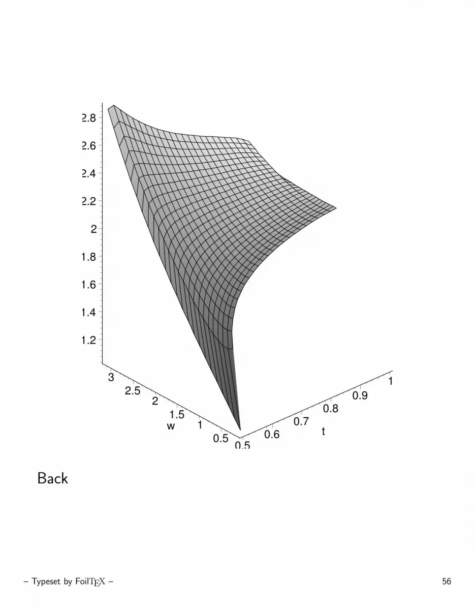
However, determining the maximal values for Φ and Ψ seems tobe a nontrivial task. It appears, though, that both functions areincreasing with respect to ω, and that Φ obtaines its maximum valueat Φ(π, 1/2, 0) as Ψ obtains its maximum at Ψ(π, 0.5056).

Then we would get

P =π

log 3≈ 2.8596 and Q ≈ 2.8854,

which yields the estimate stated in the theorem.


Open questions

1. In Theorem 3.12 the constant 1/ sin(ϕ/2) + 1 can probably beimproved in the following way; given x, y ∈ Sϕ, and letting

f : Sϕ → H2 be a power map, an estimate for the geodesicJ [x, y] is given by f−1J ′, where J ′ is the hyperbolic geodesicJ ′ = J [f(x), f(y)] in H2. Could this actually be the geodesicitself?

2. Probably ABn∗ = π/ log 3. Using better estimates for the

geodesics for just some nasty points would prove this. What dothe geodesics themselves look like?

3. Could some uniformity constant estimate be proved for a triangle,or for other polygonal domains using the result for the angle?

4. What about the domains Sϕ, π < ϕ < 2π?


References

[AVV] G. Anderson, M. Vamanamurthy, M. Vuorinen: Conformal in-variants, inequalities, and quasiconformal maps. Canad. Math.Soc. Series of Monographs and Advanced Texts. A Wiley-Interscience Publication. John Wiley & Sons, Inc., New York,1997.

[BE] A. F. Beardon: The geometry of discrete groups. Gradu-ate Texts in Mathematics, Vol. 91, Springer-Verlag, Berlin-Heidelberg-New York, 1982.

[GE] F. W. Gehring: Characteristic properties of quasidisks. LesPresses de l’Universite de Montreal, Montreal, 1982.

[GO] F. W. Gehring and B. G. Osgood: Uniform domains and thequasi-hyperbolic metric. J. Analyse Math. 36 (1979), 50–74.

[MA] G. Martin: Quasiconformal and bilipschitz mappings, uniformdomains and the hyperbolic metric. Trans. Amer. Math. Soc.292 (1985), 169–192.


[MO] G. Martin and B. G. Osgood: The quasihyperbolic metric andthe associated estimates on the hyperbolic metric. J. AnalyseMath. 47 (1986), 37–53.

[MS] O. Martio and J. Sarvas: Injectivity theorems in plane andspace. Ann. Acad. Sci. Fenn. Ser. A I Math. 4, (1978/79), 383–401.

[VU1] M. Vuorinen: Conformal invariants and quasiregular map-pings. J. Analyse Math.45, (1985), 69–115.

[VU2] M. Vuorinen: Conformal geometry and quasiregular map-pings. Lecture Notes in Mathematics, Vol. 1319 Springer-Verlag, Berlin, 1988.




ϕS

B

B

x

w

l

x

y

ϕ r

r

ωy

l

lϕ/2

ω/2


Back




z

xy d(x)=d(y)


Back




0

tan

2tan1

ω/2

(ω/2)

(ω/2)∆


Back




z

p

0

x = te

(1/2)2B

B2

Cx

2


Back


0

0.1

0.2

0.3

0.4

0.5

s

00.1

0.20.3

0.40.5 t

0

0.5

1

1.5

2

2.5

Back


0.50.6

0.70.8

0.91

t0.5

11.5

22.5

3

w

1.2

1.4

1.6

1.8

2

2.2

2.4

2.6

2.8

Back


0 0.5 1 1.5 2 2.5 30

2

4

6

8

10

12

14

16

18

20

Back


Documents

Uniformity constant estimates for some elementary domains