atmosphere

Article

An Overall Uniformity Optimization Method of the SphericalIcosahedral Grid Based on the Optimal Transformation Theory

Fuli Luo, Xuesheng Zhao * , Wenbin Sun, Yalu Li and Yuanzheng Duan

�����������������

Citation: Luo, F.; Zhao, X.; Sun, W.;

Li, Y.; Duan, Y. An Overall Uniformity

Optimization Method of the Spherical

Icosahedral Grid Based on the

Optimal Transformation Theory.

Atmosphere 2021, 12, 1516. https://

doi.org/10.3390/atmos12111516

Academic Editor: Tomasz Gierczak

Received: 22 September 2021

Accepted: 14 November 2021

Published: 17 November 2021

Publisher’s Note: MDPI stays neutral

with regard to jurisdictional claims in

published maps and institutional affil-

iations.

Copyright: © 2021 by the authors.

Licensee MDPI, Basel, Switzerland.

This article is an open access article

distributed under the terms and

conditions of the Creative Commons

Attribution (CC BY) license (https://

creativecommons.org/licenses/by/

4.0/).

School of Geoscience and Surveying Engineering, China University of Mining and Technology (Beijing),D11 Xueyuan Road, Beijing 100083, China; lfl@student.cumtb.edu.cn (F.L.); swb@cumtb.edu.cn (W.S.);bqt1700205021@student.cumtb.edu.cn (Y.L.); bqt1900205059@student.cumtb.edu.cn (Y.D.)* Correspondence: zxs@cumtb.edu.cn

Abstract: The improvement of overall uniformity and smoothness of spherical icosahedral grids,the basic framework of atmospheric models, is a key to reducing simulation errors. However, most ofthe existing grid optimization methods have optimized grid from different aspects and not improvedoverall uniformity and smoothness of grid at the same time, directly affecting the accuracy andstability of numerical simulation. Although a well-defined grid with more than 12 points cannotbe constructed on a sphere, the area uniformity and the interval uniformity of the spherical gridcan be traded off to enhance extremely the overall grid uniformity and smoothness. To solve thisproblem, an overall uniformity and smoothness optimization method of the spherical icosahedralgrid is proposed based on the optimal transformation theory. The spherical cell decompositionmethod has been introduced to iteratively update the grid to minimize the spherical transportationcost, achieving an overall optimization of the spherical icosahedral grid. Experiments on the fouroptimized grids (the spring dynamics optimized grid, the Heikes and Randall optimized grid,the spherical centroidal Voronoi tessellations optimized grid and XU optimized grid) demonstratethat the grid area uniformity of our method has been raised by 22.60% of SPRG grid, −1.30% of HRgrid, 38.30% of SCVT grid and 38.20% of XU grid, and the grid interval uniformity has been improvedby 2.50% of SPRG grid, 2.80% of HR grid, 11.10% of SCVT grid and 11.00% of XU grid. Althoughthe grid uniformity of the proposed method is similar with the HR grid, the smoothness of griddeformation has been enhanced by 79.32% of grid area and 24.07% of grid length. To some extent,the proposed method may be viewed as a novel optimization approach of the spherical icosahedralgrid which can improve grid overall uniformity and smoothness of grid deformation.

Keywords: optimal transformation theory; uniform grid; optimized spherical icosahedral grid; areauniformity; interval uniformity

1. Introduction

Spherical icosahedral grid is often used as the basic framework of atmospheric models,such as the ICosahedral Nonhydrostatic model (ICON) [1–3], Models for Predication AcrossScales (MPAS) [4], the Non-hydrostatic ICosahedral Atmospheric Model (NICAM) [5],DYNAMICO [6], Ocean–Land–Atmosphere Model (OLAM) [7,8], etc. These models arewieldy used for polar lows simulation [9], monsoon simulation [10], ocean tides dissi-pation [11], etc. Recently, the Spectral Radiation Transport Model for Aerosol Speciescoupled with NICAM (NICAM-SPRINTARS) [12] has been developed for studying andsimulating atmosphere-aerosols interactions and their effects on atmospheric pollution andclimate change. Related studies include simulating the annual aerosol characteristics overChina [13], capturing the horizontal distribution of aerosol optical thickness fields [14],studying the resolution dependency of the transport process of black carbon from Siberiato Japan [15], and assimilating global aerosol vertical observations [16], among others.

The accuracy of numerical simulations is affected by the quality of the spherical icosa-hedral grid [17–19]. Low-quality grids may cause large numerical approximation errors.

Atmosphere 2021, 12, 1516. https://doi.org/10.3390/atmos12111516 https://www.mdpi.com/journal/atmosphere

Atmosphere 2021, 12, 1516 2 of 19

Some noises are leaded by slight irregularities of the grid, which the long-term simulationwill become unstable [20]. This is because nonuniform grids may bring grid imprintingin the numerical solutions and speed up their spread in meteorological models [21,22].In this way, the nonuniformity of the control volume becomes the main source of numericalsimulation error [23]. For example, the non-orthogonality of the grid edge and its dualedge, and the non-coincidence of the midpoints of the two edges increases the truncationerror of the spherical differential operators [22,23]. Grid misalignment also leads to errorsin some low-order algorithms of the spherical surface [19,24], resulting in discretization ofdifferential operators to only meet first-order convergence [17]. The grid with good qualitycan reduce the truncation error of these operators on the sphere [25].

At present, some grid optimization methods have been proposed to improve grid qual-ity and to reduce the simulation errors [26]. The spring dynamics method (i.e., the SPRingdynamics Grid optimization (SPRG) method) [27,28] is utilized to improve grid intervaluniformity and to reduce geometric variations [19]. Iga [29] found that the interval distri-butions of grids near the icosahedron vertices, optimized by the SPRG method with a zeronatural spring length (SPR0), are inversely proportional to the map factor of the Lambertconformal conic projection. An analytical transformation was proposed to stretch the gridsnear the icosahedral vertices to decrease grid aggregations [30]. Heikes and Randall [31,32](HR) have minimized the distances between the midpoints of hexagonal/pentagonal gridsedges and their dual (triangles) edges to optimize grid. Then, they have re-optimized thegrid (named tweaked grid [33]) based on previous result to avoid the hemispheric twisting,where the grid quality and the convergence of PDE operators have been further improved.Spherical Centroidal Voronoi Tessellations (SCVT) [34–36] has been put forward, in whichgrids’ centers were iteratively moved by Llyod’s method [37] to their mass centroids tominimize the distances between these two points. Xu [25] has updated iteratively gridsbased on the Laplace-Beltrami solution, and the optimization grid and SCVT grid are veryclose to each other.

Comparations have been done with the main optimization grids, such as HR grid,SCVT grid, SPRG grid, etc. for grid quality [23,33]. Some indicators, for instance the ratiosbetween minimum and maximum grid area, the ratios between minimum and maximumgrid intervals, the grid area ranges, grid interval ranges, area relative deviations, lengthrelative deviations, etc. are used to evaluate grid quality. The grid interval ratio of SPRGgrid is bigger than HR grid, that means SPRG grid’s interval uniformity is better than thatof HR grid. However, its grid area ratio and grid interval ratio are all less than the non-optimized grid (NOPT grid). Its grid quality is limited by the spring constant. When thespring constant is large, some grids near the icosahedral vertices may collapse at highresolutions. When the constant is small, grids do not collapse, but some grids near theicosahedral vertices may aggregate, such that grid intervals are shortened and the amountof calculation is increased [29]. The grid intervals by Iga [29] only be increased along thestretch paths, decreasing the regularity of the grids near the icosahedral vertices. Althougharea uniformity of HR gird has been enhanced to the most extent, its grid interval ratiois slightly smaller than SPRG grid and NOPT grid. Among these grids, the quality ofSCVT grid is the worst, its two ratios are divergent with the increasing grid resolution,and discretization accuracy of basic operator is also lowest. There is none of them beingclearly better than the others [19].

Tomita [27] has implied that simulation error appears in regions with high gradient ofgrid area and interval deviations, and the smoothness is important for high-accuracy andstable simulation [29]. The node interpolation can follow a second-order convergence ona uniform spherical grid, but if there is any deformation, it has only a first-order conver-gence [38]. The grid uniformity is also important to determine the maximum time step fornumerical integration [20] and to maintain the consistency of physical parameterizationin atmospheric simulations [23]. Meanwhile, improvement of the uniformity is helpfulfor wavelet transform to improve the compression technique for weather and climatedata [39,40]. The grid uniformity has been quantified from grid area and grid interval devi-

Atmosphere 2021, 12, 1516 3 of 19

ations in some reviews [20,23,33]. The grid area uniformity and interval uniformity are notindependent of each other. As the spherical surface is non-Euclidean, a well-defined gridwith more than 12 points, meting the two attributes simultaneously, cannot be constructedon a sphere [20]. However, the area uniformity and the interval uniformity of the sphericalgrid can be trade off to enhance extremely the overall grid uniformity and smoothness ofthe spherical distribution of the grid area and interval deviation.

The present study is devoted to the investigation of a novel grid overall uniformity andsmoothness optimization approach rooted in the optimal transportation theory. The spheri-cal cell decomposition method was introduced to iteratively update the grid to minimizethe spherical transportation cost, achieving an optimization grid. We discuss the details ofthe proposed method and its effectiveness from the grid geometry quality and numericalaccuracy. Unlike existing optimization approaches, the proposed method is optimal in thatit does not only improve the grid overall uniformity but also reduce the grid deformation,enhancing the smoothness of grid deformation. Both the smoothness of deformation anduniformity of grid interval have been greatly improved. The smoothness of grid areadeformation has also been heightened even the grid area uniformity is comparable to thoseobtained by the Heikes and Randall grid.

The rest of this paper is organized as follows: the optimal transportation theory,grid uniformity optimization method and the core algorithm are introduced in the Theoryand Methods section. The Results and Discussions section presents the comparative resultsand discussions from the grid quality and numerical accuracy. The conclusions are shownin the last section.

2. Theory and Methods

Optimal transportation theory is used for the measure-preserving mapping betweentwo probability measure spaces, such that the target probability measure is infinitely closeto the source (or true) probability measure. In all measure-preserving mappings, a mappingminimizing the transportation cost is an optimal transportation mapping [41]. Gu [41]proposed a discrete spherical optimal transportation mapping based on a purely geometricmethod and defined the measures as areas to achieve an area-preserving mapping fromthe topological sphere to the unit sphere [42,43]. The mapping is global and has beenapplied in biomedicine [44,45], face recognition [46], generative adversarial networks [47],and other fields.

Given a continuous space Rn, two subspaces with measures, (X, ψ)∈Rn and (Y, ϕ) ∈ Rn,having the same total measures, that is

∫X ψdx =

∫Y ϕdy, there is a measure-preserving

mapping T: X → Y to make ϕ(B) = ψ(T−1(B)), where B ⊂ Y, T−1(B) ⊂ X. Then the trans-portation cost can be formalized as in Equation (1):

C(T) =∫

Xc(x, T(x))dψ(x) (1)

where C: X × Y→ R is a cost function of T; Topt = argmin{C(T)} is the optimal transportationmapping.

Spherical optimal transportation mapping realizes the area-preserving mapping fromthe topological sphere to the unit sphere. There is a probability measure ψ in the con-tinuous space defined on the unit sphere and a Dirac measure ϕ = {ϕ1, ϕ2, . . . , ϕnv}corresponding to the point set {pi} ⊂ S2, which cannot be covered by any hemisphere,such that ψ(S2) = ∑nv

i=1 ϕi. A set of cells, W = {wi}, decomposing the unit sphere, that is

S2 = ∪nvi=1wi , can be found to make ϕ(wi) = ψi. Then a mapping T: wi → pi is the

optimal transportation mapping minimizing the transportation cost. The existence anduniqueness of the complete solutions in the continuous space have been proved by Gu(2013). Surfaces can be discretized by triangular meshes. The discrete spherical optimaltransportation mapping is an approximate preserved area mapping from a topologicalspherical triangular mesh to a spherical triangular mesh. A topological spherical trian-gular mesh is M {V , E, F}, with point set V = {v1, v2, . . . , vnv}, edge set E = {e1, e2, . . . , ene}

Atmosphere 2021, 12, 1516 4 of 19

and face set F = {f 1, f 2, . . . , fnf}. ∀vi ∈ V , there is a set of first-order adjacent verticesvadj = {vi1 , vi2 , . . . , viNs }, Ns is the number of first-order adjacent vertices. ∀ψi ∈ ψ, it canbe defined as one-third of total area of triangles formed by vi and vadj, its construction isillustrated in Figure 1 and its formulization is defined in Equation (2),

ψi =13

Ns

∑j=1

S∆vivjvj+1 (2)

where S is the spherical area of ∆vivjvj+1.

Atmosphere 2021, 12, x FOR PEER REVIEW  4  of  21  

 

continuous space have been proved by Gu (2013). Surfaces can be discretized by triangular 

meshes.  The  discrete  spherical  optimal  transportation mapping  is  an  approximate  pre‐

served area mapping from a topological spherical triangular mesh to a spherical triangular 

mesh. A topological spherical triangular mesh is M {V, E, F}, with point set V = {v1, v2, …, 

vnv}, edge set E = {e1, e2, …, ene} and face set F = {f1, f2, …, fnf}. ∀vi ∈ V, there is a set of first‐order adjacent vertices vadj = {

1iv , 

2iv , …, 

Nsiv }, Ns is the number of first‐order adjacent vertices. 

∀ψi ∈ ψ,  it can be defined as one‐third of total area of triangles formed by vi and vadj,  its 

construction is illustrated in Figure 1 and its formulization is defined in Equation (2), 

11

1

3 i j j

Ns

i v v vjS

  (2)

where S is the spherical area of ∆vivjvj+1. 

 

Figure 1. Area measure ψi of vi. 

There is an optimal transportation mapping T: (M, ψ) → (N, φ), such that φi = ψi and C(T) in Equation (3) is minimal, in which N {V*, E, F} is the image of M, φ is a measure set 

of N. 

2

1

1( )

2

nv

i iiC T

  (3)

Based on the point set V, a cell decomposition set W = {wi} can be constructed, where 

wi’s area is φi. When φi equals ψi, the transportation cost is minimal equal to zero. Updat‐

ing the center of cell wi as  iv   obtains the image of the approximate preserved area map‐

ping.   

Cell decomposition on a sphere is a spherical power diagram generation. There is a 

point set V = {v1, v2, …, vnv} ∈ S2 and its weight set r = {r1, r2, …, rnv} ∈ R, ci(vi, ri) is a circle on a sphere with center vi and radius ri. Spherical power distance between any point p ∉ V and ci is defined in Equation (4):   

cos ( , )pow( , )

cosi

ii

d p vp v

r   (4)

where d(∙) means the spherical great circle, pow(p, vi) is a geodesic distance between p and 

tangent point, intersection of a line through p tangent to circle and the circle, as shown in 

Figure 2. 

   

Figure 1. Area measure ψi of vi.

There is an optimal transportation mapping T: (M, ψ)→ (N, ϕ), such that ϕi = ψi andC(T) in Equation (3) is minimal, in which N {V*, E, F} is the image of M, ϕ is a measure setof N.

C(T) =12

nv

∑i=1

(ϕi − ψi)2 (3)

Based on the point set V, a cell decomposition set W = {wi} can be constructed, wherewi’s area is ϕi. When ϕi equals ψi, the transportation cost is minimal equal to zero. Updatingthe center of cell wi as v∗i obtains the image of the approximate preserved area mapping.

Cell decomposition on a sphere is a spherical power diagram generation. There is apoint set V = {v1, v2, . . . , vnv} ∈ S2 and its weight set r = {r1, r2, . . . , rnv} ∈ R, ci(vi, ri) is acircle on a sphere with center vi and radius ri. Spherical power distance between any pointp

Atmosphere 2021, 12, x FOR PEER REVIEW  4  of  21  

 

continuous space have been proved by Gu (2013). Surfaces can be discretized by triangular 

meshes.  The  discrete  spherical  optimal  transportation mapping  is  an  approximate  pre‐

served area mapping from a topological spherical triangular mesh to a spherical triangular 

mesh. A topological spherical triangular mesh is M {V, E, F}, with point set V = {v1, v2, …, 

vnv}, edge set E = {e1, e2, …, ene} and face set F = {f1, f2, …, fnf}. ∀vi ∈ V, there is a set of first‐order adjacent vertices vadj = {

1iv , 

2iv , …, 

Nsiv }, Ns is the number of first‐order adjacent vertices. 

∀ψi ∈ ψ,  it can be defined as one‐third of total area of triangles formed by vi and vadj,  its 

construction is illustrated in Figure 1 and its formulization is defined in Equation (2), 

11

1

3 i j j

Ns

i v v vjS

  (2)

where S is the spherical area of ∆vivjvj+1. 

 

Figure 1. Area measure ψi of vi. 

There is an optimal transportation mapping T: (M, ψ) → (N, φ), such that φi = ψi and C(T) in Equation (3) is minimal, in which N {V*, E, F} is the image of M, φ is a measure set 

of N. 

2

1

1( )

2

nv

i iiC T

  (3)

Based on the point set V, a cell decomposition set W = {wi} can be constructed, where 

wi’s area is φi. When φi equals ψi, the transportation cost is minimal equal to zero. Updat‐

ing the center of cell wi as  iv   obtains the image of the approximate preserved area map‐

ping.   

Cell decomposition on a sphere is a spherical power diagram generation. There is a 

point set V = {v1, v2, …, vnv} ∈ S2 and its weight set r = {r1, r2, …, rnv} ∈ R, ci(vi, ri) is a circle on a sphere with center vi and radius ri. Spherical power distance between any point p ∉ V and ci is defined in Equation (4):   

cos ( , )pow( , )

cosi

ii

d p vp v

r   (4)

where d(∙) means the spherical great circle, pow(p, vi) is a geodesic distance between p and 

tangent point, intersection of a line through p tangent to circle and the circle, as shown in 

Figure 2. 

   

V and ci is defined in Equation (4):

pow(p, vi) =cos d(p, vi)

cos ri(4)

where d(·) means the spherical great circle, pow(p, vi) is a geodesic distance between p andtangent point, intersection of a line through p tangent to circle and the circle, as shown inFigure 2.

Atmosphere 2021, 12, x FOR PEER REVIEW  5  of  21  

 

 

Figure 2. Spherical power distance. 

The  spherical power diagram of  {(pi,  ri)}  is a cell decomposition of  sphere,  that  is 2

1

nv

iiS w

, where wi = {vi ∈ V | pow(p, vi) < pow(p, vj),  vj ∈ V−{vi}}. A spherical power 

diagram of a random point set is shown in Figure 3. 

 

Figure 3. Spherical power diagram. 

Where the green circle is spherical circle of each point with center vi and radius ri, the 

red spherical polygon is spherical power cell of each point, and the blue spherical triangle 

is cell’s dual triangle. 

It has been proved that the optimal transportation mapping can be achieved by ad‐

justing the weight of the spherical power diagram. When the area of each power cell is 

equal  the predefined weight, defined by  the area measure,  the optimal  transportation 

mapping can be obtained. According to the spherical power diagram, the transportation 

cost can be defined as follows:   

2

1

1( ) ( ( ))

2

nv

i iiC h

h   (5)

where h is a function of radius, h = −ln(cos(r)), φ is the power cell area. 

The power cell area is an analytic function of radius [42]. Let q is a center point of line 

between vi and vj, there is pow (q, vi) = pow (q, vj) (Figure 4), then:   

cos ( , ) cos ( , ) jihh

i jd q v e d q v e 

(6)

Figure 2. Spherical power distance.

Atmosphere 2021, 12, 1516 5 of 19

The spherical power diagram of {(pi, ri)} is a cell decomposition of sphere, that isS2 = ∪nv

i=1wi, where wi = {vi ∈ V | pow(p, vi) < pow(p, vj), ∀vj ∈ V−{vi}}. A spherical powerdiagram of a random point set is shown in Figure 3.

Atmosphere 2021, 12, x FOR PEER REVIEW  5  of  21  

 

 

Figure 2. Spherical power distance. 

The  spherical power diagram of  {(pi,  ri)}  is a cell decomposition of  sphere,  that  is 2

1

nv

iiS w

, where wi = {vi ∈ V | pow(p, vi) < pow(p, vj),  vj ∈ V−{vi}}. A spherical power 

diagram of a random point set is shown in Figure 3. 

 

Figure 3. Spherical power diagram. 

Where the green circle is spherical circle of each point with center vi and radius ri, the 

red spherical polygon is spherical power cell of each point, and the blue spherical triangle 

is cell’s dual triangle. 

It has been proved that the optimal transportation mapping can be achieved by ad‐

justing the weight of the spherical power diagram. When the area of each power cell is 

equal  the predefined weight, defined by  the area measure,  the optimal  transportation 

mapping can be obtained. According to the spherical power diagram, the transportation 

cost can be defined as follows:   

2

1

1( ) ( ( ))

2

nv

i iiC h

h   (5)

where h is a function of radius, h = −ln(cos(r)), φ is the power cell area. 

The power cell area is an analytic function of radius [42]. Let q is a center point of line 

between vi and vj, there is pow (q, vi) = pow (q, vj) (Figure 4), then:   

cos ( , ) cos ( , ) jihh

i jd q v e d q v e 

(6)

Figure 3. Spherical power diagram.

Where the green circle is spherical circle of each point with center vi and radius ri,the red spherical polygon is spherical power cell of each point, and the blue sphericaltriangle is cell’s dual triangle.

It has been proved that the optimal transportation mapping can be achieved byadjusting the weight of the spherical power diagram. When the area of each power cellis equal the predefined weight, defined by the area measure, the optimal transportationmapping can be obtained. According to the spherical power diagram, the transportationcost can be defined as follows:

C(h) =12

nv

∑i=1

(ϕ(ω(hi))− ψi)2

(5)

where h is a function of radius, h = −ln(cos(r)), ϕ is the power cell area.The power cell area is an analytic function of radius [42]. Let q is a center point of line

between vi and vj, there is pow (q, vi) = pow (q, vj) (Figure 4), then:

cos d(q, vi)ehi = cos d(q, vj)ehj (6)

Atmosphere 2021, 12, x FOR PEER REVIEW  6  of  21  

 

 

Figure 4. Power cell and its dual triangle. 

Where Rl and Rk are triangle power radius of ∆vivjvk and ∆vivjvl.. dl and dk are vertical 

distances from the triangle center ol and ok to edge [vi, vj], respectively. γi and γj are the 

distances between vi and q, vj and q, respectively. 

Let γi = d(q, vi), γj = d(q, vj), and γi+γj = γij, there is:   

cos( ) cos jihh

ij j je e  

(7)

1tan = ( cos )

sinj ih h

j jij

e

 

(8)

According to the partial derivative of tanγj with respect to hi, there is:   

2 2

2 2 2

tan 1=cos = cos

sin

cos1 1= (cos ) = cos cos ( )

sin sin cos

j i

j i j

h hj jj j

i i ij

h h h lj i j

ij ij l

de

dh h

Re e r r

d

 

(9)

According  to area of  infinitesimal  spherical quadrilateral,  jli   = area(wi  ∩ ∆vivjvl), 

jki   = area(wi ∩ ∆vivjvk), φ is the power cell area. There is: 

2

2

cos sincos cos

sin cosjk l l

i ji ij l

R dr r

h d

  (10)

2

2

cos sincos cos

sin cos

iki k k

i jj ij k

R dr r

h d

  (11)

2 2

2 2

cos cos cos sin cos sin

sin cos cosj i ji l l k k

j i ij l k

r r R d R d

h h d d

  (12)

The convexity of the transportation cost has been proved by Gu (2013) and it can be 

minimized by means of Newton’s method. The gradient of cost can be defined as ∇C = (φ(w1) −  1, φ(w2) −  2, …, φ(wnv) −  nv), and the Hessian matrix can be expressed as fol‐

lows:   

Figure 4. Power cell and its dual triangle.

Atmosphere 2021, 12, 1516 6 of 19

Where Rl and Rk are triangle power radius of ∆vivjvk and ∆vivjvl.. dl and dk are verticaldistances from the triangle center ol and ok to edge [vi, vj], respectively. γi and γj are thedistances between vi and q, vj and q, respectively.

Let γi = d(q, vi), γj = d(q, vj), and γi + γj = γij, there is:

cos(γij − γj)ehi = cos γjehj (7)

tan γj =1

sin γij(ehj−hi − cos γj) (8)

According to the partial derivative of tanγj with respect to hi, there is:

dγjdhi

= cos2 γj∂ tan γj

∂hi= − cos2 γj

1sin γij

ehj−hi

= − 1sin γij

e−hj−hi (cos2 γjehj)

2= − 1

sin γijcos ri cos rj(

cos Rlcos dl

)2 (9)

According to area of infinitesimal spherical quadrilateral, ϕjli = area(wi ∩ ∆vivjvl),

ϕjki = area(wi ∩ ∆vivjvk), ϕ is the power cell area. There is:

∂ϕjk

∂hi= − cos2 Rl sin dl

sin γij cos2 dlcos ri cos rj (10)

∂ϕiki

∂hj= − cos2 Rk sin dk

sin γij cos2 dkcos ri cos rj (11)

∂ϕi∂hj

=∂ϕj

∂hi= −

cos ri cos rj

sin γij

(cos2 Rl sin dl

cos2 dl+

cos2 Rk sin dkcos2 dk

)(12)

The convexity of the transportation cost has been proved by Gu (2013) and it canbe minimized by means of Newton’s method. The gradient of cost can be defined as∇C = (ϕ(w1)−ψ1, ϕ(w2)−ψ2, . . . , ϕ(wnv)−ψnv), and the Hessian matrix can be expressedas follows:

H =

− ∑i 6=1

∂ϕi∂h1

∂ϕ2∂h1

. . . ∂ϕnv∂h1

∂ϕ1∂h2

− ∑i 6=2

∂ϕi∂h2

· · · ∂ϕnv∂h2

......

. . ....

∂ϕ1∂hnv

∂ϕ2∂hnv

· · · − ∑i 6=nv

∂ϕi∂hnv

(13)

For the spherical icosahedral grid, the measure-preserving mapping becomes a self-mapping. The measure is replaced by a virtual measure ψvirtual, where ψi_virtual = 4πR2/nvfor any spherical icosahedral grid point; R is the earth radius. There is a mapping T:(Ico-Grid, ψvirtual)→ (AREA-Ico-Grid, ϕ), where Ico-Grid is composed of a grid point setV = {vi}, a grid edge set E, a grid set F and a grid point set of AREA-Ico-Grid, V* = {v∗i }is the image of V under the mapping T, its grid edge set and grid set are the same asIco-Grid’s. When the areas of the grids by cell decomposition are equal to each other, that isϕ(v*) = ψvirtual(T−1(v*)), v* ⊂ AREA-Ico-Grid, T−1(v*) ⊂ Ico-Grid, T is the approximatearea-preserved mapping. The Algorithm 1 of area quasi-uniformity optimization for thespherical icosahedral grid is described as follows.

Atmosphere 2021, 12, 1516 7 of 19

Algorithm 1: Area Uniformity Optimization for the Spherical Icosahedral Grid

Input: a spherical icosahedral grid Ico-Grid {V , E, F}, step λ, initial height vector h0, threshold δCOutput: a spherical icosahedral grid with area quasi-uniformity AREA-Ico-Grid {V*, E, F}(1) Compute the virtual measure ψvirtual = {ψi_virtual};(2) According to h0 and V , decompose the sphere into a cell set W = {wi}, and calculate eachpower cell area to get the original measure ϕ of Ico-Grid by, ϕ0 ←ϕ;(3) Calculate the transportation cost C between ϕ0 and ψvirtual by Equation (3). If C < δC, V*← Vand move to step 5. If not, move to the next step;(4) Update cell decomposition of S2

(4.1) Calculate gradient ∇C = (ϕ(w1) − ψ1, ϕ(w2) − ψ2, . . . , ϕ(wnv) − ψnv)T;(4.2) Compute the transportation cost C via∇C. If C<δC, move to step 5. If not, move to step 4.3;(4.3) According to Equations (10)–(13), calculate a Hessian matrix H;(4.4) Establish the relationship between hessian matrix and gradient, that is Hδh = ∇C;(4.5) Update height vector, h = h + λδh;(4.6) Decompose the sphere into a new cell set W = {wi} based on h; compute cells’ area ϕW = {ϕwi};

(5) Compute the centers of cells in W, and obtain CW = {cwi};(6) V*← CW, and output result;(7) End.

3. Results and Discussions

To verify the effectiveness of this algorithm, tests were performed to compare the gridquality and numerical accuracy among the proposed algorithm optimized grid (OURSgrid), the non-optimized grid (NOPT grid), the spring dynamic method optimized grid(SPRG grid), tweaked grid optimized by Heikes and Randall grid (HR grid) SphericalCentroidal Voronoi Tessellations grid (SCVT grid) and grid optimized by Xu (XU grid).Here, the construction of the NOPT grid was through recursive division, and the parameterβ in the SPRG grid was set to 1.1 according to [33]. All experiments were implemented inC++ and executed on a PC with Intel Core i5-6400 CPU@2.70 GHz, 8 GB RAM.

3.1. The Grid Quality Evaluation3.1.1. The Grid Area Uniformity

The relative area deviation Darea was used to measure the grid area uniformity, whichcan be calculated with Equation (14):

Darea =A− Aavg

Aavg(14)

where A is the area of a grid; Aavg is the average area of the spherical icosahedral grid;earth radius was set to 6, 371.007 km.

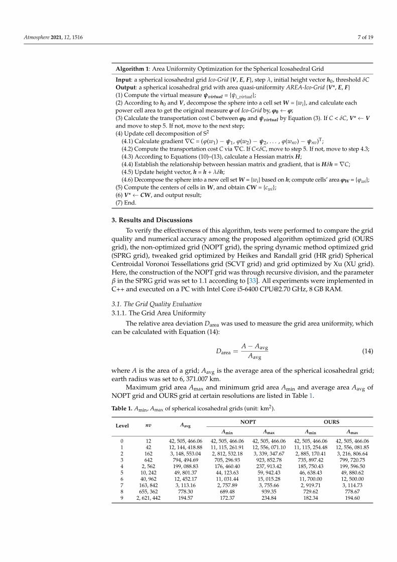
Maximum grid area Amax and minimum grid area Amin and average area Aavg ofNOPT grid and OURS grid at certain resolutions are listed in Table 1.

Table 1. Amin, Amax of spherical icosahedral grids (unit: km2).

Level nv AavgNOPT OURS

Amin Amax Amin Amax

0 12 42, 505, 466.06 42, 505, 466.06 42, 505, 466.06 42, 505, 466.06 42, 505, 466.061 42 12, 144, 418.88 11, 115, 261.91 12, 556, 071.10 11, 115, 254.48 12, 556, 081.852 162 3, 148, 553.04 2, 812, 532.18 3, 339, 347.67 2, 885, 170.41 3, 216, 806.643 642 794, 494.69 705, 296.93 923, 852.78 735, 897.42 799, 720.754 2, 562 199, 088.83 176, 460.40 237, 913.42 185, 750.43 199, 596.505 10, 242 49, 801.37 44, 123.63 59, 942.43 46, 638.43 49, 880.626 40, 962 12, 452.17 11, 031.44 15, 015.28 11, 700.00 12, 500.007 163, 842 3, 113.16 2, 757.89 3, 755.66 2, 919.71 3, 114.738 655, 362 778.30 689.48 939.35 729.62 778.679 2, 621, 442 194.57 172.37 234.84 182.34 194.60

Atmosphere 2021, 12, 1516 8 of 19

The grid area was normalized according to Equation (15) to compare the differencesat various resolutions.

A =A× nv12× R2 (15)

The normalized minimum area Amin and maximum area Amax of different sphericalicosahedral grids are listed in Table 2, and their curves are illustrated in Figure 5. Ratios be-tween the minimum and maximum area, rA = Amin/Amax, of different spherical icosahedralgrids at different resolutions are presented in Figure 6.

Table 2. The normalized area and the ratios between the Amin and Amax.

Level 3 4 5 6 7 8 9

Aavg 1.047 1.047 1.047 1.047 1.047 1.047 1.047

NOPTAmin 0.930 0.928 0.930 0.928 0.928 0.928 0.928Amax 1.218 1.251 1.260 1.263 1.263 1.264 1.264

rA 0.764 0.742 0.740 0.735 0.735 0.734 0.734

SPRGAmin 0.879 0.848 0.820 0.803 0.791 0.781 0.776Amax 1.080 1.079 1.080 1.081 1.083 1.087 1.092

rA 0.814 0.786 0.760 0.743 0.730 0.718 0.711

HRAmin 0.998 1.008 1.012 1.014 1.013 1.016 1.016Amax 1.062 1.066 1.068 1.068 1.069 1.070 1.070

rA 0.940 0.946 0.950 0.949 0.948 0.950 0.950

SCVTAmin 0.861 0.812 0.760 0.719 0.677 0.639 0.599Amax 1.082 1.081 1.080 1.081 1.081 1.081 1.081

rA 0.796 0.751 0.710 0.665 0.626 0.591 0.554

XUAmin 0.861 0.812 0.760 0.719 0.676 0.638 0.600Amax 1.082 1.081 1.080 1.081 1.082 1.082 1.082

rA 0.796 0.751 0.710 0.665 0.625 0.590 0.555

OURSAmin 0.970 0.977 0.981 0.984 0.982 0.982 0.981Amax 1.054 1.050 1.049 1.051 1.048 1.048 1.047

rA 0.920 0.930 0.940 0.936 0.937 0.937 0.937

Atmosphere 2021, 12, x FOR PEER REVIEW  9  of  21  

 

HR 

minA   0.998  1.008  1.012  1.014  1.013  1.016  1.016 

maxA   1.062  1.066  1.068  1.068  1.069  1.070  1.070 

rA  0.940  0.946  0.950  0.949  0.948  0.950  0.950 

SCVT 

minA   0.861  0.812  0.760  0.719  0.677  0.639  0.599 

maxA   1.082  1.081  1.080  1.081  1.081  1.081  1.081 

rA  0.796  0.751  0.710  0.665  0.626  0.591  0.554 

XU 

minA   0.861  0.812  0.760  0.719  0.676  0.638  0.600 

maxA   1.082  1.081  1.080  1.081  1.082  1.082  1.082 

rA  0.796  0.751  0.710  0.665  0.625  0.590  0.555 

OURS 

minA   0.970  0.977  0.981  0.984  0.982  0.982  0.981 

maxA   1.054  1.050  1.049  1.051  1.048  1.048  1.047 

rA  0.920  0.930  0.940  0.936  0.937  0.937  0.937 

 

Figure 5.  minA   and  maxA   of different grids. 

 

Figure 6. Ratios between Amin and Amax of different grids. 

The maximum grid area, minimum grid area and their ratios indicate the ranges of grid 

area. The closer the ratio  is  to one,  the smaller the area range  is, which  indicates a more 

uniform grid area. The normalized minimum and maximum areas of all grids except the 

SCVT grid and XU grid gradually have converged as the resolution increases (Figures 5 and 

6 and Tables 1 and 2). The area range of SCVT grid and XU grid are the same and the biggest 

among all grids at  level 9. The one of NOPT grid  is  followed and  that of HR grid  is  the 

smallest. The range of OURS grid is only expanded by 1.20% compared with HR grid. Same 

as the range, ratios of SCVT grid and XU grid are non‐convergence as resolution increases 

and have decreased to 0.554 and 0.555 at level 9, respectively. The ratios of SPRG grid and 

NOPT grid have converged slowly to 0.711 and 0.734, respectively. On the contrary, the ones 

of HR grid and OURS grid have increased as resolution increases and converged to 0.950 

and 0.937, respectively at the same resolution. 

Figure 5. Amin and Amax of different grids.

Atmosphere 2021, 12, x FOR PEER REVIEW  9  of  21  

 

HR 

minA   0.998  1.008  1.012  1.014  1.013  1.016  1.016 

maxA   1.062  1.066  1.068  1.068  1.069  1.070  1.070 

rA  0.940  0.946  0.950  0.949  0.948  0.950  0.950 

SCVT 

minA   0.861  0.812  0.760  0.719  0.677  0.639  0.599 

maxA   1.082  1.081  1.080  1.081  1.081  1.081  1.081 

rA  0.796  0.751  0.710  0.665  0.626  0.591  0.554 

XU 

minA   0.861  0.812  0.760  0.719  0.676  0.638  0.600 

maxA   1.082  1.081  1.080  1.081  1.082  1.082  1.082 

rA  0.796  0.751  0.710  0.665  0.625  0.590  0.555 

OURS 

minA   0.970  0.977  0.981  0.984  0.982  0.982  0.981 

maxA   1.054  1.050  1.049  1.051  1.048  1.048  1.047 

rA  0.920  0.930  0.940  0.936  0.937  0.937  0.937 

 

Figure 5.  minA   and  maxA   of different grids. 

 

Figure 6. Ratios between Amin and Amax of different grids. 

The maximum grid area, minimum grid area and their ratios indicate the ranges of grid 

area. The closer the ratio  is  to one,  the smaller the area range  is, which  indicates a more 

uniform grid area. The normalized minimum and maximum areas of all grids except the 

SCVT grid and XU grid gradually have converged as the resolution increases (Figures 5 and 

6 and Tables 1 and 2). The area range of SCVT grid and XU grid are the same and the biggest 

among all grids at  level 9. The one of NOPT grid  is  followed and  that of HR grid  is  the 

smallest. The range of OURS grid is only expanded by 1.20% compared with HR grid. Same 

as the range, ratios of SCVT grid and XU grid are non‐convergence as resolution increases 

and have decreased to 0.554 and 0.555 at level 9, respectively. The ratios of SPRG grid and 

NOPT grid have converged slowly to 0.711 and 0.734, respectively. On the contrary, the ones 

of HR grid and OURS grid have increased as resolution increases and converged to 0.950 

and 0.937, respectively at the same resolution. 

Figure 6. Ratios between Amin and Amax of different grids.

Atmosphere 2021, 12, 1516 9 of 19

The maximum grid area, minimum grid area and their ratios indicate the ranges ofgrid area. The closer the ratio is to one, the smaller the area range is, which indicatesa more uniform grid area. The normalized minimum and maximum areas of all gridsexcept the SCVT grid and XU grid gradually have converged as the resolution increases(Figures 5 and 6 and Tables 1 and 2). The area range of SCVT grid and XU grid are the sameand the biggest among all grids at level 9. The one of NOPT grid is followed and that of HRgrid is the smallest. The range of OURS grid is only expanded by 1.20% compared with HRgrid. Same as the range, ratios of SCVT grid and XU grid are non-convergence as resolutionincreases and have decreased to 0.554 and 0.555 at level 9, respectively. The ratios ofSPRG grid and NOPT grid have converged slowly to 0.711 and 0.734, respectively. On thecontrary, the ones of HR grid and OURS grid have increased as resolution increases andconverged to 0.950 and 0.937, respectively at the same resolution.

To further emphasize the spherical distribution characteristic of grid area uniformity,taking the grid at level 9 as an example, the number of grids in different intervals of gridarea relative deviation calculated by Equation (15) are counted in Table 3.

Table 3. The number of grids in different Darea interval of different grids.

Interval (%) NOPT SPRG HR SCVT XU OURS

[−100, −38.0] 0 0 0 0 0 0(−38.0, −34.0) 0 0 0 162 162 0(−34.0, −30.0) 0 0 0 0 0 0(−30.0, −26.0) 0 0 0 960 960 0(−26.0, −22.0) 0 162 0 1, 920 1, 920 0(−22.0, −18.0) 0 960 0 2, 880 3, 840 0(−18.0, −14.0) 0 4, 800 0 14, 400 13, 440 0(−14.0, −10.0) 192 34, 560 0 42, 240 42, 240 0(−10.0, −6.0) 436, 770 180, 480 0 112, 320 115, 200 12(−6.0, −2.0) 1, 132, 800 630, 720 22, 786 314, 880 317, 760 0(−2.0, 2.0) 366, 240 887, 520 2598, 480 1, 403, 040 1, 341, 584 2, 621, 430(2.0, 6.0) 60, 480 647, 040 176 728, 640 784, 336 0(6.0, 10.0) 0 235, 200 0 0 0 0

(10.0, 14.0) 380, 160 0 0 0 0 0(14.0, 18.0) 96, 000 0 0 0 0 0(18.0, 22.0) 148, 800 0 0 0 0 0(22.0, 100.0) 0 0 0 0 0 0

total 2, 621, 442 2, 621, 442 2, 621, 442 2, 621, 442 2, 621, 442 2, 621, 442

Refine these intervals to further demonstrate the area features of OURS grid (Table 4).Where, N is the number of grids in different intervals, and p is grid proportions.

The cumulative grid proportions of |Darea| are depicted in Table 5, and Figure 7(|Darea| < 0.08%).

The Darea of all grids are in [−38.0%, 22.0%] (Table 3). The ones of HR grid and OURSgrid are mainly in (−2.0%, 2.0%), which is smaller than other four grids. There are morethan 90% grids with Darea in (−0.06%, 0.06%) in OURS grid. The cumulative proportionshave increased logarithmically as |Darea| increases, in which the increasing rate of OURSgrid is the fastest and that of NOPT grid is the slowest (Figure 7). The cumulative propor-tions of OURS grid with |Darea| of less than 0.044% is more than 90.00%, and the ones ofother five grids are only 0.02% (NOPT grid), 0.62% (SPRG grid), 13.24% (HR grid), 0.37%(SCVT grid), and 1.25% (XU grid). Although the area ratio of HR grid is bigger than OURSgrid, the proportion of grid with smaller is far less than that of OURS grid.

Meanwhile, the spherical distributions of the area relative deviations at level 9 areshown in Figure 8, where the lighter the color is, the closer the grid area deviation is tozero.

Atmosphere 2021, 12, 1516 10 of 19

Table 4. The number of grids in refined Darea interval of OURS grid.

Interval (%) N p (%)

[−100, −0.18) 72 0.00[−0.18, −0.14) 60 0.00[−0.14, −0.10) 17, 695 0.68[−0.10, −0.06) 44, 733 1.71[−0.06, −0.02) 495, 834 18.91[−0.02, 0.02) 1, 342, 129 51.20(−0.02, 0.60) 720, 919 27.50

(0.06, 100] 0 0total 2, 621, 442 100.00

Table 5. The cumulative proportion of |Darea| of different grids (%).

Interval (%) NOPT SPRG HR SCVT XU OURS

[0, 0.004) 0 0 1.07 0 0.26 12.57[0.004, 0.012) 0.02 0.07 3.27 0.07 0.59 33.35[0.012, 0.02) 0.02 0.22 5.87 0.07 0.73 51.20[0.02, 0.028) 0.02 0.22 8.63 0.22 0.93 66.98[0.028, 0.036) 0.02 0.51 11.06 0.22 1.25 81.04[0.036, 0.044) 0.02 0.62 13.24 0.37 1.25 92.56[0.044, 0.052) 0.02 0.77 15.10 0.66 1.39 96.17[0.052, 0.06) 0.02 0.99 16.73 0.92 1.39 97.61[0.06, 0.068) 0.02 1.65 22.95 2.38 1.76 99.32[0.068, 0.076) 0.02 2.23 28.11 3.04 2.16 99.99

[0.076, 0.3) 0.02 4.69 43.54 6.23 5.35 99.99[0.3, 0.5) 0.02 7.87 56.64 10.25 9.87 99.99[0.5, 0.7) 0.02 11.17 66.66 14.39 14.25 99.99[0.7, 0.9) 0.02 14.39 74.64 18.82 18.53 99.99[0.9, 2) 13.97 33.86 99.12 53.52 51.18 99.99[6, 26) 59.49 82.6 100 93.33 93.32 100

[26, 100] 100 100 100 100 100 100

Atmosphere 2021, 12, x FOR PEER REVIEW  11  of  21  

 

[0.044, 0.052)  0.02  0.77  15.10  0.66  1.39  96.17 

[0.052, 0.06)  0.02  0.99  16.73  0.92  1.39  97.61 

[0.06, 0.068)  0.02  1.65  22.95  2.38  1.76  99.32 

[0.068, 0.076)  0.02  2.23  28.11  3.04  2.16  99.99 

[0.076, 0.3)  0.02  4.69  43.54  6.23  5.35  99.99 

[0.3, 0.5)  0.02  7.87  56.64  10.25  9.87  99.99 

[0.5, 0.7)  0.02  11.17  66.66  14.39  14.25  99.99 

[0.7, 0.9)  0.02  14.39  74.64  18.82  18.53  99.99 

[0.9, 2)  13.97  33.86  99.12  53.52  51.18  99.99 

[6, 26)  59.49  82.6  100  93.33  93.32  100 

[26, 100]  100  100  100  100  100  100 

 

Figure 7. Curves of cumulative proportion for different grids at level 9 (|Darea| < 0.08%). 

The Darea of all grids are in [−38.0%, 22.0%] (Table 3). The ones of HR grid and OURS 

grid are mainly in (−2.0%, 2.0%), which is smaller than other four grids. There are more 

than 90% grids with Darea in (−0.06%, 0.06%) in OURS grid. The cumulative proportions 

have increased logarithmically as |Darea| increases, in which the increasing rate of OURS 

grid is the fastest and that of NOPT grid is the slowest (Figure 7). The cumulative propor‐

tions of OURS grid with |Darea| of less than 0.044% is more than 90.00%, and the ones of 

other five grids are only 0.02% (NOPT grid), 0.62% (SPRG grid), 13.24% (HR grid), 0.37% 

(SCVT grid), and 1.25% (XU grid). Although the area ratio of HR grid is bigger than OURS 

grid, the proportion of grid with smaller is far less than that of OURS grid. 

Meanwhile, the spherical distributions of the area relative deviations at level 9 are 

shown in Figure 8, where the lighter the color is, the closer the grid area deviation is to 

zero.   

(a)  (b)  (c) 

Figure 7. Curves of cumulative proportion for different grids at level 9 (|Darea| < 0.08%).

From Figure 8, the grids with maximum area deviation are the pentagons, and spher-ical distributions patterns of Darea are symmetry. The distribution of NOPT grid hasfractal characteristics and is not continuous. Because of the larger number of grids withlarger Darea, its distribution is shown by darker color. The distributions of the SPRG grid,SCVT grid and XU grid are similar. As the larger number of grids with smaller Darea(−0.06%, 0.06%) in OURS grid, its distribution is shown by the lightest color and somegrids with larger Darea are mainly located along the triangular boundaries. Grids withlarger Darea are also located around these boundaries, however, these regions are far largerthan that of OURS grid.

Atmosphere 2021, 12, 1516 11 of 19

Atmosphere 2021, 12, x FOR PEER REVIEW  11  of  21  

 

[0.044, 0.052)  0.02  0.77  15.10  0.66  1.39  96.17 

[0.052, 0.06)  0.02  0.99  16.73  0.92  1.39  97.61 

[0.06, 0.068)  0.02  1.65  22.95  2.38  1.76  99.32 

[0.068, 0.076)  0.02  2.23  28.11  3.04  2.16  99.99 

[0.076, 0.3)  0.02  4.69  43.54  6.23  5.35  99.99 

[0.3, 0.5)  0.02  7.87  56.64  10.25  9.87  99.99 

[0.5, 0.7)  0.02  11.17  66.66  14.39  14.25  99.99 

[0.7, 0.9)  0.02  14.39  74.64  18.82  18.53  99.99 

[0.9, 2)  13.97  33.86  99.12  53.52  51.18  99.99 

[6, 26)  59.49  82.6  100  93.33  93.32  100 

[26, 100]  100  100  100  100  100  100 

 

Figure 7. Curves of cumulative proportion for different grids at level 9 (|Darea| < 0.08%). 

The Darea of all grids are in [−38.0%, 22.0%] (Table 3). The ones of HR grid and OURS 

grid are mainly in (−2.0%, 2.0%), which is smaller than other four grids. There are more 

than 90% grids with Darea in (−0.06%, 0.06%) in OURS grid. The cumulative proportions 

have increased logarithmically as |Darea| increases, in which the increasing rate of OURS 

grid is the fastest and that of NOPT grid is the slowest (Figure 7). The cumulative propor‐

tions of OURS grid with |Darea| of less than 0.044% is more than 90.00%, and the ones of 

other five grids are only 0.02% (NOPT grid), 0.62% (SPRG grid), 13.24% (HR grid), 0.37% 

(SCVT grid), and 1.25% (XU grid). Although the area ratio of HR grid is bigger than OURS 

grid, the proportion of grid with smaller is far less than that of OURS grid. 

Meanwhile, the spherical distributions of the area relative deviations at level 9 are 

shown in Figure 8, where the lighter the color is, the closer the grid area deviation is to 

zero.   

(a)  (b)  (c) 

Atmosphere 2021, 12, x FOR PEER REVIEW  12  of  21  

 

(d)  (e)  (f) 

Figure 8. Spherical distributions of Darea of different grids at level 9. (a) NOPT grid. (b) SPRG grid. 

(c) HR grid. (d) SCVT grid. (e) XU grid. (f) OURS grid. 

From Figure 8, the grids with maximum area deviation are the pentagons, and spher‐

ical distributions patterns of Darea are symmetry. The distribution of NOPT grid has fractal 

characteristics and is not continuous. Because of the larger number of grids with larger 

Darea, its distribution is shown by darker color. The distributions of the SPRG grid, SCVT 

grid and XU grid are similar. As the larger number of grids with smaller Darea (−0.06%, 

0.06%) in OURS grid, its distribution is shown by the lightest color and some grids with 

larger Darea are mainly located along the triangular boundaries. Grids with larger Darea are 

also located around these boundaries, however, these regions are far larger than that of 

OURS grid. 

3.1.2. The Grid Interval Uniformity 

The geodesic distance, d, between grid points, the minimum distance, dmin and the 

maximum distance dmax (Table 6), the ratios between them (Table 7) and the grid length 

relative deviation (as Equation (16)) are calculated to describe the grid interval uniformity.   

avg

lengthavg

L LD

L

  (16)

Table 6. dmin, dmax, davg of different grids (unit: km). 

Level NOPT  OURS 

davg  dmin  dmax  davg  dmin  dmax 

0  7529.85  7529.85  7529.85  7529.85  7529.85  7529.85 

1  3764.92  3526.83  4003.02  3764.92  3526.83  4003.02 

2  1914.33  1763.41  2079.28  1915.30  1739.23  2087.62 

3  961.22  881.71  1050.16  961.85  866.34  1059.12 

4  481.12  440.85  526.42  481.47  432.15  532.56 

5  240.62  220.43  263.38  240.81  215.84  267.18 

6  120.32  110.21  131.71  120.42  107.83  134.40 

7  60.16  55.11  65.86  60.20  54.13  67.12 

8  30.08  27.55  32.93  30.10  27.06  33.56 

9  15.04  13.78  16.47  15.05  13.53  16.78 

Table 7. Normalized distance and ratios between the dmin and dmax of different grids. 

Level  3  4  5  6  7  8  9 

avgd  1.182  1.182  1.182  1.182  1.182  1.182  1.182 

NOPT 

mind   1.107  1.107  1.107  1.107  1.107  1.107  1.107 

maxd   1.319  1.322  1.323  1.323  1.323  1.323  1.323 

rd  0.839  0.837  0.837  0.837  0.837  0.837  0.837 

Figure 8. Spherical distributions of Darea of different grids at level 9. (a) NOPT grid. (b) SPRG grid. (c) HR grid. (d) SCVTgrid. (e) XU grid. (f) OURS grid.

3.1.2. The Grid Interval Uniformity

The geodesic distance, d, between grid points, the minimum distance, dmin and themaximum distance dmax (Table 6), the ratios between them (Table 7) and the grid lengthrelative deviation (as Equation (16)) are calculated to describe the grid interval uniformity.

Dlength =L− Lavg

Lavg(16)

Table 6. dmin, dmax, davg of different grids (unit: km).

LevelNOPT OURS

davg dmin dmax davg dmin dmax

0 7529.85 7529.85 7529.85 7529.85 7529.85 7529.85

1 3764.92 3526.83 4003.02 3764.92 3526.83 4003.02

2 1914.33 1763.41 2079.28 1915.30 1739.23 2087.62

3 961.22 881.71 1050.16 961.85 866.34 1059.12

4 481.12 440.85 526.42 481.47 432.15 532.56

5 240.62 220.43 263.38 240.81 215.84 267.18

6 120.32 110.21 131.71 120.42 107.83 134.40

7 60.16 55.11 65.86 60.20 54.13 67.12

8 30.08 27.55 32.93 30.10 27.06 33.56

9 15.04 13.78 16.47 15.05 13.53 16.78

Atmosphere 2021, 12, 1516 12 of 19

Table 7. Normalized distance and ratios between the dmin and dmax of different grids.

Level 3 4 5 6 7 8 9

davg 1.182 1.182 1.182 1.182 1.182 1.182 1.182

NOPTdmin 1.107 1.107 1.107 1.107 1.107 1.107 1.107dmax 1.319 1.322 1.323 1.323 1.323 1.323 1.323

rd 0.839 0.837 0.837 0.837 0.837 0.837 0.837

SPRGdmin 1.077 1.059 1.043 1.017 1.017 0.999 0.983dmax 1.276 1.279 1.279 1.284 1.285 1.279 1.259

rd 0.844 0.828 0.815 0.802 0.791 0.781 0.781

HRdmin 1.076 1.074 1.074 1.074 1.074 1.074 1.075dmax 1.351 1.361 1.364 1.364 1.365 1.364 1.382

rd 0.796 0.789 0.787 0.787 0.787 0.787 0.778

SCVTdmin 1.065 1.035 1.005 0.975 0.946 0.917 0.890dmax 1.275 1.277 1.277 1.277 1.277 1.277 1.280

rd 0.835 0.810 0.787 0.763 0.741 0.718 0.695

XUdmin 1.065 1.035 1.005 0.975 0.945 0.916 0.888dmax 1.275 1.277 1.277 1.277 1.277 1.277 1.276

rd 0.835 0.810 0.787 0.763 0.740 0.717 0.696

OURSdmin 1.088 1.085 1.084 1.083 1.087 1.091 1.091dmax 1.330 1.337 1.342 1.350 1.349 1.354 1.353

rd 0.818 0.812 0.808 0.802 0.806 0.806 0.806

The grid distance was normalized according to Equation (17) to compare the differ-ences at various resolutions (Table 7 and Figure 9).

d =d× 2Level

R(17)

Atmosphere 2021, 12, x FOR PEER REVIEW  13  of  21  

 

SPRG 

mind   1.077  1.059  1.043  1.017  1.017  0.999  0.983 

maxd   1.276  1.279  1.279  1.284  1.285  1.279  1.259 

rd  0.844  0.828  0.815  0.802  0.791  0.781  0.781 

HR 

mind   1.076  1.074  1.074  1.074  1.074  1.074  1.075 

maxd   1.351  1.361  1.364  1.364  1.365  1.364  1.382 

rd  0.796  0.789  0.787  0.787  0.787  0.787  0.778 

SCVT 

mind   1.065  1.035  1.005  0.975  0.946  0.917  0.890 

maxd   1.275  1.277  1.277  1.277  1.277  1.277  1.280 

rd  0.835  0.810  0.787  0.763  0.741  0.718  0.695 

XU 

mind   1.065  1.035  1.005  0.975  0.945  0.916  0.888 

maxd   1.275  1.277  1.277  1.277  1.277  1.277  1.276 

rd  0.835  0.810  0.787  0.763  0.740  0.717  0.696 

OURS 

mind   1.088  1.085  1.084  1.083  1.087  1.091  1.091 

maxd   1.330  1.337  1.342  1.350  1.349  1.354  1.353 

rd  0.818  0.812  0.808  0.802  0.806  0.806  0.806 

The grid distance was normalized according to Equation (17) to compare the differ‐

ences at various resolutions (Table 7 and Figure 9).   

2Leveldd

R

  (17)

 

Figure 9. The normalized minimum and maximum distance of different grids. 

Ratios between the minimum and maximum distances, rd=dmin/dmax, of different grids 

at different resolutions are calculated in Table 7 and presented in Figure 10. 

 

Figure 10. Ratios between minimum and maximum distance of different grids. 

Figure 9. The normalized minimum and maximum distance of different grids.

Ratios between the minimum and maximum distances, rd = dmin/dmax, of differentgrids at different resolutions are calculated in Table 7 and presented in Figure 10.

Same as the normalized area, dmin, dmax and ratios indicate the ranges of grid interval.The closer the ratio is to one, the smaller the interval range is, which indicates a moreuniform grid interval. The dmin, dmax of the all grids except the SCVT grid and XU gridhave gradually converged as the resolution increases (Figures 9 and 10 and Tables 6 and 7).The ratios of SCVT grid and XU grid are non-convergence as resolution increases, and onesof SPRG grid and HR grid have converged to 0.781 and 0.778 at level 9, respectively,the ratio of OURS grid is larger than them.

The number of grids in different intervals of grid length relative deviation have beencounted (Table 8) to emphasize the spherical distribution characteristic of grid intervaluniformity.

Atmosphere 2021, 12, 1516 13 of 19

Atmosphere 2021, 12, x FOR PEER REVIEW  13  of  21  

 

SPRG 

mind   1.077  1.059  1.043  1.017  1.017  0.999  0.983 

maxd   1.276  1.279  1.279  1.284  1.285  1.279  1.259 

rd  0.844  0.828  0.815  0.802  0.791  0.781  0.781 

HR 

mind   1.076  1.074  1.074  1.074  1.074  1.074  1.075 

maxd   1.351  1.361  1.364  1.364  1.365  1.364  1.382 

rd  0.796  0.789  0.787  0.787  0.787  0.787  0.778 

SCVT 

mind   1.065  1.035  1.005  0.975  0.946  0.917  0.890 

maxd   1.275  1.277  1.277  1.277  1.277  1.277  1.280 

rd  0.835  0.810  0.787  0.763  0.741  0.718  0.695 

XU 

mind   1.065  1.035  1.005  0.975  0.945  0.916  0.888 

maxd   1.275  1.277  1.277  1.277  1.277  1.277  1.276 

rd  0.835  0.810  0.787  0.763  0.740  0.717  0.696 

OURS 

mind   1.088  1.085  1.084  1.083  1.087  1.091  1.091 

maxd   1.330  1.337  1.342  1.350  1.349  1.354  1.353 

rd  0.818  0.812  0.808  0.802  0.806  0.806  0.806 

The grid distance was normalized according to Equation (17) to compare the differ‐

ences at various resolutions (Table 7 and Figure 9).   

2Leveldd

R

  (17)

 

Figure 9. The normalized minimum and maximum distance of different grids. 

Ratios between the minimum and maximum distances, rd=dmin/dmax, of different grids 

at different resolutions are calculated in Table 7 and presented in Figure 10. 

 

Figure 10. Ratios between minimum and maximum distance of different grids. Figure 10. Ratios between minimum and maximum distance of different grids.

Table 8. The number of grids with different Dlength interval of different grids.

NOPT SPRG HR SCVT XU OURS

[−100, −15] 0 0 0 0 0 0(−15, −13] 0 0 0 60 60 0(−13, −11] 0 0 0 120 120 0(−11, −9] 0 0 0 360 420 0(−9, −7] 0 5, 730 0 720 1, 020 0(−7, −5] 0 28, 800 0 2, 640 2, 280 0(−5, −3] 0 151, 680 0 100, 800 106, 030 0(−3, −1] 1, 488, 960 620, 160 0 301, 632 301, 632 0(−1, 1) 446, 880 966, 240 2, 447, 056 1, 536, 160 1, 471, 680 2, 621, 430[1, 3) 60, 480 679, 680 174, 374 678, 950 738, 200 0[3, 5) 0 168, 960 0 0 0 0[5, 7) 446, 400 192 0 0 0 0[7, 9) 144, 960 0 0 0 0 0

[9, 11) 33, 750 0 0 0 0 0[11, 13) 0 0 0 0 0 0[13, 15) 0 0 0 0 0 0[15, 17) 12 0 0 0 0 0[17, 19) 0 0 0 0 0 12[19, 21) 0 0 12 0 0 0

[21, 100] 0 0 0 0 0 0total 2, 621, 442 2, 621, 442 2, 621, 442 2, 621, 442 2, 621, 442 2, 621, 442

There are the similar characteristics of HR and OURS grid from Table 8, so the intervalsis refined to further reveal their differences in Table 9. Where, N is the number of grids indifferent intervals, and p is grid proportions.

Table 9. The number of grids with refined Dlength interval of HR and OURS grid.

Interval (%)HR OURS

N p (%) N p (%)

[−100, −1.1] 16 0.00 0 0(−1.1, −0.9] 46, 592 1.78 0 0(−0.9, −0.7] 137, 776 5.26 0 0(−0.7, −0.5] 835, 680 31.88 0 0(−0.5, −0.3] 468, 576 17.87 325, 328 12.41(−0.3, −0.1] 288, 704 11.01 659, 536 25.16

(−0.1,0.1) 211, 232 8.06 676, 512 25.81[0.1, 0.3) 166, 432 6.35 705, 728 26.92[0.3, 0.5) 134, 192 5.12 234, 528 8.95[0.5, 0.7) 110, 118 4.20 19, 798 0.76[0.7, 0.9) 91, 328 3.48 0 0[0.9, 1.0) 73, 328 2.80 0 0[1.1, 1.3) 50, 640 1.93 0 0

Atmosphere 2021, 12, 1516 14 of 19

Table 9. Cont.

Interval (%)HR OURS

N p (%) N p (%)

[1.3, 1.5) 6, 816 0.26 0 0[1.5, 1.7) 0 0 0 0[1.7, 2.3) 0 0 12 0[2.3, 100] 12 0 0 0

total 2, 621, 442 100 2, 621, 442 100

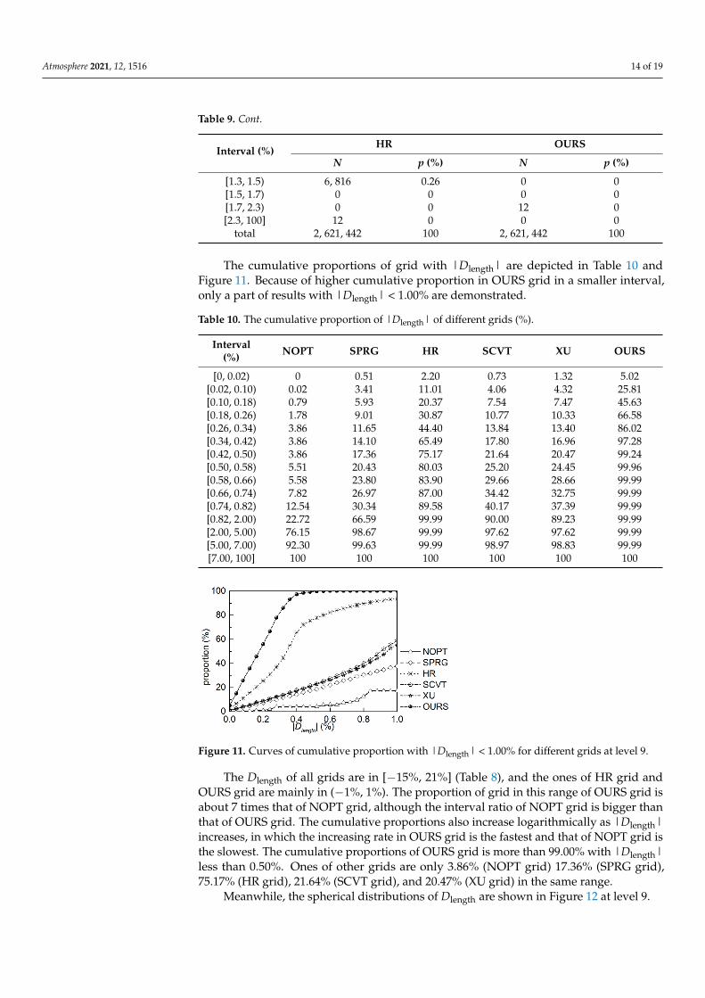
The cumulative proportions of grid with |Dlength| are depicted in Table 10 andFigure 11. Because of higher cumulative proportion in OURS grid in a smaller interval,only a part of results with |Dlength| < 1.00% are demonstrated.

Table 10. The cumulative proportion of |Dlength| of different grids (%).

Interval(%) NOPT SPRG HR SCVT XU OURS

[0, 0.02) 0 0.51 2.20 0.73 1.32 5.02[0.02, 0.10) 0.02 3.41 11.01 4.06 4.32 25.81[0.10, 0.18) 0.79 5.93 20.37 7.54 7.47 45.63[0.18, 0.26) 1.78 9.01 30.87 10.77 10.33 66.58[0.26, 0.34) 3.86 11.65 44.40 13.84 13.40 86.02[0.34, 0.42) 3.86 14.10 65.49 17.80 16.96 97.28[0.42, 0.50) 3.86 17.36 75.17 21.64 20.47 99.24[0.50, 0.58) 5.51 20.43 80.03 25.20 24.45 99.96[0.58, 0.66) 5.58 23.80 83.90 29.66 28.66 99.99[0.66, 0.74) 7.82 26.97 87.00 34.42 32.75 99.99[0.74, 0.82) 12.54 30.34 89.58 40.17 37.39 99.99[0.82, 2.00) 22.72 66.59 99.99 90.00 89.23 99.99[2.00, 5.00) 76.15 98.67 99.99 97.62 97.62 99.99[5.00, 7.00) 92.30 99.63 99.99 98.97 98.83 99.99[7.00, 100] 100 100 100 100 100 100

Atmosphere 2021, 12, x FOR PEER REVIEW  15  of  21  

 

[0.5, 0.7)  110, 118  4.20  19, 798  0.76 

[0.7, 0.9)  91, 328  3.48  0  0 

[0.9, 1.0)  73, 328  2.80  0  0 

[1.1, 1.3)  50, 640  1.93  0  0 

[1.3, 1.5)  6, 816  0.26  0  0 

[1.5, 1.7)  0  0  0  0 

[1.7, 2.3)  0  0  12  0 

[2.3, 100]  12  0  0  0 

total  2, 621, 442  100  2, 621, 442  100 

The cumulative proportions of grid with |Dlength| are depicted in Table 10 and   

Figure 11. Because of higher cumulative proportion in OURS grid in a smaller interval, 

only a part of results with |Dlength| < 1.00% are demonstrated. 

Table 10. The cumulative proportion of |Dlength| of different grids (%). 

Interval (%)  NOPT  SPRG  HR  SCVT  XU  OURS 

[0, 0.02)  0  0.51  2.20  0.73  1.32  5.02 

[0.02, 0.10)  0.02  3.41  11.01  4.06  4.32  25.81 

[0.10, 0.18)  0.79  5.93  20.37  7.54  7.47  45.63 

[0.18, 0.26)  1.78  9.01  30.87  10.77  10.33  66.58 

[0.26, 0.34)  3.86  11.65  44.40  13.84  13.40  86.02 

[0.34, 0.42)  3.86  14.10  65.49  17.80  16.96  97.28 

[0.42, 0.50)  3.86  17.36  75.17  21.64  20.47  99.24 

[0.50, 0.58)  5.51  20.43  80.03  25.20  24.45  99.96 

[0.58, 0.66)  5.58  23.80  83.90  29.66  28.66  99.99 

[0.66, 0.74)  7.82  26.97  87.00  34.42  32.75  99.99 

[0.74, 0.82)  12.54  30.34  89.58  40.17  37.39  99.99 

[0.82, 2.00)  22.72  66.59  99.99  90.00  89.23  99.99 

[2.00, 5.00)  76.15  98.67  99.99  97.62  97.62  99.99 

[5.00, 7.00)  92.30  99.63  99.99  98.97  98.83  99.99 

[7.00, 100]  100  100  100  100  100  100 

 

Figure 11. Curves of cumulative proportion with |Dlength| < 1.00% for different grids at level 9. 

The Dlength of all grids are in [−15%, 21%] (Table 8), and the ones of HR grid and OURS 

grid are mainly in (−1%, 1%). The proportion of grid in this range of OURS grid is about 7 

times that of NOPT grid, although the interval ratio of NOPT grid is bigger than that of 

OURS  grid.  The  cumulative  proportions  also  increase  logarithmically  as  |Dlength|  in‐

creases, in which the increasing rate in OURS grid is the fastest and that of NOPT grid is 

the slowest. The cumulative proportions of OURS grid is more than 99.00% with |Dlength| 

Figure 11. Curves of cumulative proportion with |Dlength| < 1.00% for different grids at level 9.

The Dlength of all grids are in [−15%, 21%] (Table 8), and the ones of HR grid andOURS grid are mainly in (−1%, 1%). The proportion of grid in this range of OURS grid isabout 7 times that of NOPT grid, although the interval ratio of NOPT grid is bigger thanthat of OURS grid. The cumulative proportions also increase logarithmically as |Dlength|increases, in which the increasing rate in OURS grid is the fastest and that of NOPT grid isthe slowest. The cumulative proportions of OURS grid is more than 99.00% with |Dlength|less than 0.50%. Ones of other grids are only 3.86% (NOPT grid) 17.36% (SPRG grid),75.17% (HR grid), 21.64% (SCVT grid), and 20.47% (XU grid) in the same range.

Meanwhile, the spherical distributions of Dlength are shown in Figure 12 at level 9.

Atmosphere 2021, 12, 1516 15 of 19

Atmosphere 2021, 12, x FOR PEER REVIEW  16  of  21  

 

less  than 0.50%. Ones of other grids are only 3.86%  (NOPT grid) 17.36%  (SPRG grid), 

75.17% (HR grid), 21.64% (SCVT grid), and 20.47% (XU grid) in the same range. 

Meanwhile, the spherical distributions of Dlength are shown in Figure 12 at level 9.   

(a)  (b)  (c) 

(d)  (e)  (f) 

Figure 12. Spherical distributions of Dlength at level 9. (a) NOPT grid. (b) SPRG grid. (c) HR grid. (d) 

SCVT grid. (e) XU grid. (f) OURS grid 

Same as spherical distribution of grid area, the grids with maximum Dlength are these 

pentagons, and distributions of all grids are symmetry. Near these pentagons, the lengths 

of grids are less than the average length and shown by darker color in all grids. The dis‐

tribution of NOPT grid has fractal characteristics and is not continuous, too. The Dlength in 

the remaining grids are reduced from the pentagons to triangular centers. The grids with 

larger Dlength are mainly located along the triangular boundaries in OURS grid, and those 

grids are spread like pentagon or star from these pentagons.   

3.2. The Numerical Accuracy Evaluation 

Spherical Laplacian operators of scalar field (as Equation (18)) is discretized to eval‐

uate numerical accuracy on different grids.   

4( , ) cos cosf   (18)

where λ and 𝜑 are the longitude and latitude of point on the sphere, respectively. The L2‐norm error (as Equation (19)), L∞‐norm error (as Equation (20)) of discretiza‐

tion have been calculated (Tables 11 and 12 and Figures 13 and 14). 

2num ana2 1

1

1 nv

i i inv i

ii

L A f fA

  (19)

num ana

1,max i ii nv

L f f   (19)

where  fana and  fnum are the analytical and numerical solutions of Laplacian operator, re‐

spectively. 

   

Figure 12. Spherical distributions of Dlength at level 9. (a) NOPT grid. (b) SPRG grid. (c) HR grid. (d) SCVT grid. (e) XUgrid. (f) OURS grid.

Same as spherical distribution of grid area, the grids with maximum Dlength arethese pentagons, and distributions of all grids are symmetry. Near these pentagons,the lengths of grids are less than the average length and shown by darker color in allgrids. The distribution of NOPT grid has fractal characteristics and is not continuous, too.The Dlength in the remaining grids are reduced from the pentagons to triangular centers.The grids with larger Dlength are mainly located along the triangular boundaries in OURSgrid, and those grids are spread like pentagon or star from these pentagons.

3.2. The Numerical Accuracy Evaluation

Spherical Laplacian operators of scalar field (as Equation (18)) is discretized to evaluatenumerical accuracy on different grids.

f (λ, ϕ) = cos λ× cos4 ϕ (18)

where λ and ϕ are the longitude and latitude of point on the sphere, respectively.The L2-norm error (as Equation (19)), L∞-norm error (as Equation (20)) of discretization

have been calculated (Tables 11 and 12 and Figures 13 and 14).

L2 =

√√√√( 1∑nv

i=1 Ai

(nv

∑i=1

Ai(

f numi − f ana

i)2))

(19)

L∞ = maxi=1,nv

| f numi − f ana

i | (20)

where f ana and f num are the analytical and numerical solutions of Laplacian operator,respectively.

Table 11. L2-norm error of Laplacian operator of different grids.

2 3 4 5 6 7 8

NOPT 1.31 × 10−1 3.78 × 10−2 1.20 × 10−2 4.49 × 10−3 1.96 × 10−3 9.26 × 10−4 4.52 × 10−4

SPRG 1.33 × 10−1 3.56 × 10−2 9.47 × 10−3 2.74 × 10−3 9.30 × 10−4 3.84 × 10−4 1.47 × 10−4

HR 1.41 × 10−1 3.79 × 10−2 9.85 × 10−3 2.58 × 10−3 7.23 × 10−4 2.05 × 10−4 6.05 × 10−5

SCVT 1.33 × 10−1 3.55 × 10−2 9.47 × 10−3 2.81 × 10−3 1.04 × 10−3 4.61 × 10−4 2.23 × 10−4

XU 1.33 × 10−1 3.55 × 10−2 9.47 × 10−3 2.81 × 10−3 1.04 × 10−3 4.61 × 10−4 2.23 × 10−4

OURS 1.38 × 10−1 3.75 × 10−2 9.78 × 10−3 2.57 × 10−3 6.98 × 10−4 1.99 × 10−4 5.42 × 10−5

Atmosphere 2021, 12, 1516 16 of 19

Table 12. L∞-norm error of Laplacian operator of different grids.

2 3 4 5 6 7 8

NOPT 3.52 × 10−1 1.28 × 10−1 8.08 × 10−2 8.89 × 10−2 9.10 × 10−2 9.10 × 10−2 9.15 × 10−2

SPRG 2.81 × 10−1 7.62 × 10−2 3.56 × 10−2 3.23 × 10−2 3.00 × 10−2 2.70 × 10−2 2.57 × 10−2

HR 2.84 × 10−1 8.67 × 10−2 3.23 × 10−2 1.41 × 10−2 6.75 × 10−3 3.31 × 10−3 1.66 × 10−3

SCVT 2.81 × 10−1 7.61 × 10−2 3.92 × 10−2 3.88 × 10−2 3.87 × 10−2 3.87 × 10−2 3.87 × 10−2

XU 2.81 × 10−1 7.61 × 10−2 3.92 × 10−2 3.88 × 10−2 3.87 × 10−2 3.87 × 10−2 3.87 × 10−2

OURS 2.85 × 10−1 7.81 × 10−2 2.93 × 10−2 1.35 × 10−2 6.59 × 10−3 3.27 × 10−3 1.59 × 10−3

Atmosphere 2021, 12, x FOR PEER REVIEW  17  of  21  

 

Table 11. L2‐norm error of Laplacian operator of different grids. 

  2  3  4  5  6  7  8 

NOPT  1.31 × 10−1 3.78 × 10−2 1.20 × 10−2  4.49 × 10−3  1.96 × 10−3  9.26 × 10−4  4.52 × 10−4 

SPRG  1.33 × 10−1 3.56 × 10−2 9.47 × 10−3  2.74 × 10−3  9.30 × 10−4  3.84 × 10−4  1.47 × 10−4 

HR  1.41 × 10−1 3.79 × 10−2 9.85 × 10−3  2.58 × 10−3  7.23 × 10−4  2.05 × 10−4  6.05 × 10−5 

SCVT  1.33 × 10−1 3.55 × 10−2 9.47 × 10−3  2.81 × 10−3  1.04 × 10−3  4.61 × 10−4  2.23 × 10−4 

XU  1.33 × 10−1 3.55 × 10−2 9.47 × 10−3  2.81 × 10−3  1.04 × 10−3  4.61 × 10−4  2.23 × 10−4 

OURS  1.38 × 10−1 3.75 × 10−2 9.78 × 10−3  2.57 × 10−3  6.98 × 10−4  1.99 × 10−4  5.42 × 10−5 

Table 12. L∞‐norm error of Laplacian operator of different grids. 

  2  3  4  5  6  7  8 

NOPT  3.52 × 10−1  1.28 × 10−1  8.08 × 10−2  8.89 × 10−2  9.10 × 10−2  9.10 × 10−2  9.15 × 10−2 

SPRG  2.81 × 10−1  7.62 × 10−2  3.56 × 10−2  3.23 × 10−2  3.00 × 10−2  2.70 × 10−2  2.57 × 10−2 

HR  2.84 × 10−1  8.67 × 10−2  3.23 × 10−2  1.41 × 10−2  6.75 × 10−3  3.31 × 10−3  1.66 × 10−3 

SCVT  2.81 × 10−1  7.61 × 10−2  3.92 × 10−2  3.88 × 10−2  3.87 × 10−2  3.87 × 10−2  3.87 × 10−2 

XU  2.81 × 10−1  7.61 × 10−2  3.92 × 10−2  3.88 × 10−2  3.87 × 10−2  3.87 × 10−2  3.87 × 10−2 

OURS  2.85 × 10−1  7.81 × 10−2  2.93 × 10−2  1.35 × 10−2  6.59 × 10−3  3.27 × 10−3  1.59 × 10−3 

 

Figure 13. L2‐norm error of Laplacian operator. (a) L2‐norm error of all grids (b) L2‐norm error of 

OURS and HR grid from level 5 to 8 

 

Figure 14. L∞‐norm error of Laplacian operator. (a) L∞‐norm error of all grids (b) L∞‐norm error of 

OURS and HR grid from level 5 to 8 

The L2‐norm errors and L∞‐norm errors of all grids have been reduced as resolution 

increase, ones of OURS grid and HR grid are smaller than the others. The L∞‐norm error 

(meaning the maximal error) of OURS grid has been reduced from 9.15 × 10−2 (NOPT grid), 

2.57 × 10−2 (SPRG grid), 1.66 × 10−2 (HR grid), 3.87 × 10−2 (SCVT and XU grid) to 1.59 × 10−2 

at  level 8. The L2‐norm error (meaning the RMS error) of OURS grid has been reduced 

(a)  (b) 

(a)  (b) 

Figure 13. L2-norm error of Laplacian operator. (a) L2-norm error of all grids (b) L2-norm error ofOURS and HR grid from level 5 to 8.

Atmosphere 2021, 12, x FOR PEER REVIEW  17  of  21  

 

Table 11. L2‐norm error of Laplacian operator of different grids. 

  2  3  4  5  6  7  8 

NOPT  1.31 × 10−1 3.78 × 10−2 1.20 × 10−2  4.49 × 10−3  1.96 × 10−3  9.26 × 10−4  4.52 × 10−4 

SPRG  1.33 × 10−1 3.56 × 10−2 9.47 × 10−3  2.74 × 10−3  9.30 × 10−4  3.84 × 10−4  1.47 × 10−4 

HR  1.41 × 10−1 3.79 × 10−2 9.85 × 10−3  2.58 × 10−3  7.23 × 10−4  2.05 × 10−4  6.05 × 10−5 

SCVT  1.33 × 10−1 3.55 × 10−2 9.47 × 10−3  2.81 × 10−3  1.04 × 10−3  4.61 × 10−4  2.23 × 10−4 

XU  1.33 × 10−1 3.55 × 10−2 9.47 × 10−3  2.81 × 10−3  1.04 × 10−3  4.61 × 10−4  2.23 × 10−4 

OURS  1.38 × 10−1 3.75 × 10−2 9.78 × 10−3  2.57 × 10−3  6.98 × 10−4  1.99 × 10−4  5.42 × 10−5 

Table 12. L∞‐norm error of Laplacian operator of different grids. 

  2  3  4  5  6  7  8 

NOPT  3.52 × 10−1  1.28 × 10−1  8.08 × 10−2  8.89 × 10−2  9.10 × 10−2  9.10 × 10−2  9.15 × 10−2 

SPRG  2.81 × 10−1  7.62 × 10−2  3.56 × 10−2  3.23 × 10−2  3.00 × 10−2  2.70 × 10−2  2.57 × 10−2 

HR  2.84 × 10−1  8.67 × 10−2  3.23 × 10−2  1.41 × 10−2  6.75 × 10−3  3.31 × 10−3  1.66 × 10−3 

SCVT  2.81 × 10−1  7.61 × 10−2  3.92 × 10−2  3.88 × 10−2  3.87 × 10−2  3.87 × 10−2  3.87 × 10−2 

XU  2.81 × 10−1  7.61 × 10−2  3.92 × 10−2  3.88 × 10−2  3.87 × 10−2  3.87 × 10−2  3.87 × 10−2 

OURS  2.85 × 10−1  7.81 × 10−2  2.93 × 10−2  1.35 × 10−2  6.59 × 10−3  3.27 × 10−3  1.59 × 10−3 

 

Figure 13. L2‐norm error of Laplacian operator. (a) L2‐norm error of all grids (b) L2‐norm error of 

OURS and HR grid from level 5 to 8 

 

Figure 14. L∞‐norm error of Laplacian operator. (a) L∞‐norm error of all grids (b) L∞‐norm error of 

OURS and HR grid from level 5 to 8 

The L2‐norm errors and L∞‐norm errors of all grids have been reduced as resolution 

increase, ones of OURS grid and HR grid are smaller than the others. The L∞‐norm error 

(meaning the maximal error) of OURS grid has been reduced from 9.15 × 10−2 (NOPT grid), 

2.57 × 10−2 (SPRG grid), 1.66 × 10−2 (HR grid), 3.87 × 10−2 (SCVT and XU grid) to 1.59 × 10−2 

at level 8. The L2‐norm error (meaning the RMS error) of OURS grid has been reduced 

(a)  (b) 

(a)  (b) 

Figure 14. L∞-norm error of Laplacian operator. (a) L∞-norm error of all grids (b) L∞-norm error ofOURS and HR grid from level 5 to 8.

The L2-norm errors and L∞-norm errors of all grids have been reduced as resolutionincrease, ones of OURS grid and HR grid are smaller than the others. The L∞-normerror (meaning the maximal error) of OURS grid has been reduced from 9.15 × 10−2

(NOPT grid), 2.57× 10−2 (SPRG grid), 1.66× 10−2 (HR grid), 3.87× 10−2 (SCVT and XU grid)to 1.59× 10−2 at level 8. The L2-norm error (meaning the RMS error) of OURS grid has beenreduced from 4.52 × 10−4 (NOPT grid), 2.03 × 10−4 (SPRG grid), 6.05 × 10−5 (HR grid),2.33 × 10−4 (SCVT and XU grid) to 5.86 × 10−4 at the same grid resolution, in which theenhancement of average accuracy is nearly 8 times that of NOPT grid and has more than11.62% compared to the HR grid.

Meanwhile, the spherical distributions of the Laplacian operator error on differentgrids are shown in Figure 15 at level 5.

Grids in NOPT grid with larger errors are mainly located the boundaries of refinedicosahedral triangular cells, and that of all optimization grids are mainly located on theicosahedral triangular boundaries. In OURS grid, there are some fluctuations near icosahe-dral vertices and the middle part of boundaries, grids’ error in these regions are smallerthan that of HR grid. In addition, the error range of OURS grid is the smallest among allgrids, and it has been narrowed to 84.81% of NOPT grid and 12.00% of HR grid.

Atmosphere 2021, 12, 1516 17 of 19

Atmosphere 2021, 12, x FOR PEER REVIEW  18  of  21  

 

from 4.52 × 10−4  (NOPT grid), 2.03 × 10−4  (SPRG grid), 6.05 × 10−5  (HR grid), 2.33 × 10−4 

(SCVT and XU grid) to 5.86 × 10−4 at the same grid resolution, in which the enhancement 

of average accuracy is nearly 8 times that of NOPT grid and has more than 11.62% com‐

pared to the HR grid.   

Meanwhile, the spherical distributions of the Laplacian operator error on different 

grids are shown in Figure 15 at level 5. 

(a)  (b)  (c) 

(d)  (e)  (f) 

Figure 15. Spherical distributions of Laplacian operator error of different grids. (a) NOPT grid. (b) 

SPRG grid. (c) HR grid. (d) SCVT grid. (e) XU grid. (f) OURS grid. 

Grids in NOPT grid with larger errors are mainly located the boundaries of refined 

icosahedral triangular cells, and that of all optimization grids are mainly located on the 

icosahedral triangular boundaries. In OURS grid, there are some fluctuations near icosa‐

hedral vertices and the middle part of boundaries, grids’ error in these regions are smaller 

than that of HR grid. In addition, the error range of OURS grid is the smallest among all 

grids, and it has been narrowed to 84.81% of NOPT grid and 12.00% of HR grid. 

3.3. Discussion 

The raw grid (non‐optimized grid) has been optimized by the proposed method. The 

area quasi‐uniformity can be achieved by minimizing the grid area deviation cost, which 

improve  the smoothness of grid area deviation  to some extent. Although  the grid area 

range of OURS grid is comparable to those of Heikes and Randall grid, the deformations 

of grid area and intervals of OURS grid are smoother, which is conducive to error control 

in simulation. In addition, the maximum error and RMS error of discritization of Lapla‐

cian operator have been decreased and converged as the resolution increases.   

The grid quality is one of the aspects affecting the simulation accuracy. There is no 

high gradient of grid area and interval deformation in the optimized grid by our method, 

which can be helpful to improve the accuracy of discritization of Laplacian operator. A 

more extensive analysis of Laplace operator in a diffusion problem and some numerical 

experiments in terms of the accuracy and the numerical efficiency will be carried out in 

the future. 

4. Conclusions 

In  this  study,  an overall uniformity  and  smoothness  optimization method  of  the 

spherical icosahedral grid has been proposed based on the optimal transportation theory. 

The  effectiveness  of  the  proposed  method  was  evaluated  for  grid  uniformity  and 

Figure 15. Spherical distributions of Laplacian operator error of different grids. (a) NOPT grid. (b) SPRG grid. (c) HR grid.(d) SCVT grid. (e) XU grid. (f) OURS grid.

3.3. Discussion

The raw grid (non-optimized grid) has been optimized by the proposed method.The area quasi-uniformity can be achieved by minimizing the grid area deviation cost,which improve the smoothness of grid area deviation to some extent. Although the gridarea range of OURS grid is comparable to those of Heikes and Randall grid, the deforma-tions of grid area and intervals of OURS grid are smoother, which is conducive to errorcontrol in simulation. In addition, the maximum error and RMS error of discritization ofLaplacian operator have been decreased and converged as the resolution increases.

The grid quality is one of the aspects affecting the simulation accuracy. There is nohigh gradient of grid area and interval deformation in the optimized grid by our method,which can be helpful to improve the accuracy of discritization of Laplacian operator.A more extensive analysis of Laplace operator in a diffusion problem and some numericalexperiments in terms of the accuracy and the numerical efficiency will be carried out in thefuture.

4. Conclusions

In this study, an overall uniformity and smoothness optimization method of thespherical icosahedral grid has been proposed based on the optimal transportation theory.The effectiveness of the proposed method was evaluated for grid uniformity and smooth-ness and the following conclusions may be drawn: (1) the area uniformity measured by theratio between minimum and maximum grid area has been improved by 22.6% (SPRG grid),38.3% (SCVT grid) and 38.2% (XU grid), and can be comparable to the HR grid. The intervaluniformity has also been increased by 2.5% (SPRG grid), 2.8% (HR grid), 11.1% (SCVT grid)and 11.0% (XU grid). (2) the smoothness of grid area deformation measured by the numberof grids with grid area deviation of less than 0.05% has been enhanced by 79.32% (HR grid)and more than 90% compared to the SPRG grid, SCVT grid and XU grid. The smoothnessof grid length deformation has also been increased by 24.07% (HR grid) and more than 75%compared to other three grids. Although the uniformity of grid optimized by the proposedmethod is comparable to the HR grid, the smoothness of grid deformation is improved.In addition, the average accuracy of Laplacian operator is slightly better than the HR grid.

In this study, we only evaluated the geometric uniformity of the optimized grid,and the truncation error of Laplacian operator. Future work will focus on the accuracy of

Atmosphere 2021, 12, 1516 18 of 19

Laplacian operator of different grids in a diffusion equation problem and some numericalexperiments in terms of the accuracy and the numerical efficiency.

Author Contributions: F.L. formed the research idea, designed and conducted the experiment,drafted the manuscript; X.Z. co-designed the research, analyzed the results and revised the manuscript;W.S. revised the manuscript; Y.L. and Y.D. contributed to the grammar modification. All authorshave read and agreed to the published version of the manuscript.

Funding: This research was funded by the National Key Research and Development Program ofChina (2018YFB0505301) and the National Natural Science Foundation of China (No. 41671394, No.41671383).

Institutional Review Board Statement: Not applicable.

Informed Consent Statement: Not applicable.

Data Availability Statement: Data set available on request to corresponding authors.

Acknowledgments: The authors would like to sincerely thank the two anonymous reviewers whoseinsightful comments have helped to substantially improve the manuscript. We would like to ac-knowledge and thank Peixoto for providing the Heikes and Randall grid and SCVT grid.

Conflicts of Interest: The authors declare no conflict of interest.

References1. Gassmann, A. A global hexagonal C-grid non-hydrostatic dynamical core (ICON-IAP) designed for energetic consistency. Q. J. R.

Meteorol. Soc. 2013, 139, 152–175. [CrossRef]2. Schubert, J.J.; Stevens, B.; Crueger, T. Madden-Julian oscillation as simulated by the MPI Earth System Model: Over the last and

into the next millennium. J. Adv. Model. Earth Syst. 2013, 5, 71–84. [CrossRef]3. Zängl, G.; Reinert, D.; Rípodas, P.; Baldauf, M. The ICON (ICOsahedral Non-hydrostatic) modelling framework of DWD and

MPI-M: Description of the non-hydrostatic dynamical core. Q. J. R. Meteorol. Soc. 2015, 141, 563–579. [CrossRef]4. Skamarock, W.C.; Klemp, J.B.; Duda, M.G.; Fowler, L.D.; Park, S.-H.; Ringler, T.D. A Multiscale Nonhydrostatic Atmospheric

Model Using Centroidal Voronoi Tesselations and C-Grid Staggering. Mon. Weather. Rev. 2012, 140, 3090–3105. [CrossRef]5. Satoh, M. Atmospheric Circulation Dynamics and General Circulation Models; Springer: Berlin/Heidelberg, Germany, 2014.6. Dubos, T.; Dubey, S.; Tort, M.; Mittal, R.; Meurdesoif, Y.; Hourdin, F. DYNAMICO-1.0, an icosahedral hydrostatic dynamical core

designed for consistency and versatility. Geosci. Model Dev. 2015, 8, 3131–3150. [CrossRef]7. Walko, R.L.; Avissar, R. The Ocean-Land-Atmosphere Model (OLAM). Part I: Shallow-Water Tests. Mon. Weather Rev. 2008, 136,

4033–4044. [CrossRef]8. Walko, R.L.; Avissar, R. The Ocean-Land-Atmosphere Model (OLAM). Part II: Formulation and Tests of the Nonhydrostatic

Dynamic Core. Mon. Weather Rev. 2008, 136, 4045–4062. [CrossRef]9. Revokatova, A.; Nikitin, M.; Rivin, G.; Rozinkina, I.; Nikitin, A.; Tatarinovich, E. High-Resolution Simulation of Polar Lows over

Norwegian and Barents Seas Using the COSMO-CLM and ICON Models for the 2019–2020 Cold Season. Atmosphere 2021, 12, 137.[CrossRef]

10. Hsu, L.-H.; Chen, D.-R.; Chiang, C.-C.; Chu, J.-L.; Yu, Y.-C.; Wu, C.-C. Simulations of the East Asian Winter Monsoon onSubseasonal to Seasonal Time Scales Using the Model for Prediction Across Scales. Atmosphere 2021, 12, 865. [CrossRef]

11. Hay, H.C.F.C.; Matsuyama, I. Nonlinear tidal dissipation in the subsurface oceans of Enceladus and other icy satellites. Icarus2018, 319, 68–85. [CrossRef]

12. Suzuki, K.; Nakajima, T.; Satoh, M.; Tomita, H.; Takemura, T.; Nakajima, T.; Stephens, G.L. Global cloud-system-resolvingsimulation of aerosol effect on warm clouds. Geophys. Res. Lett. 2008, 35, 610–616. [CrossRef]

13. Cheng, Y.; Dai, T.; Zhang, H.; Xin, J.; Chen, S.; Shi, G.; Nakajima, T. Comparison and evaluation of the simulated annual aerosolcharacteristics over China with two global aerosol models. Sci. Total Environ. 2021, 763, 143003–143017. [CrossRef] [PubMed]

14. Goto, D.; Kikuchi, M.; Suzuki, K.; Hayasaki, M.; Yoshida, M.; Nagao, T.M.; Choi, M.; Kim, J.; Sugimoto, N.; Shimizu, A.; et al.Aerosol model evaluation using two geostationary satellites over East Asia in May 2016. Atmos. Res. 2019, 217, 93–113. [CrossRef]

15. Yamashita, Y.; Takigawa, M.; Goto, D.; Yashiro, H.; Satoh, M.; Kanaya, Y.; Taketani, F.; Miyakawa, T. Effect of Model Resolution onBlack Carbon Transport from Siberia to the Arctic Associated with the Well-Developed Low-Pressure Systems in September. J.Meteorol. Soc. Jpn. 2021, 99, 287–308. [CrossRef]

16. Cheng, Y.; Dai, T.; Goto, D.; Schutgens, N.A.J.; Shi, G.; Nakajima, T. Investigating the assimilation of CALIPSO global aerosolvertical observations using a four-dimensional ensemble Kalman filter. Atmos. Chem. Phys. 2019, 19, 13445–13467. [CrossRef]

17. Korn, P. Formulation of an unstructured grid model for global ocean dynamics. J. Comput. Phys. 2017, 339, 525–552. [CrossRef]18. Peixoto, P.S. Accuracy analysis of mimetic finite volume operators on geodesic grids and a consistent alternative. J. Comput. Phys.

2016, 310, 127–160. [CrossRef]

Atmosphere 2021, 12, 1516 19 of 19

19. Peixoto, P.S.; Barros, S.R.M. Analysis of grid imprinting on geodesic spherical icosahedral grids. J. Comput. Phys. 2013, 237, 61–78.[CrossRef]

20. Wang, N.; Lee, J.L. Geometric Properties of the Icosahedral-Hexagonal Grid on the Two-Sphere. Soc. Ind. Appl. Math. 2011, 33,2536–2559. [CrossRef]

21. Weller, H.; Thuburn, J.; Cotter, C.J. Computational modes and grid imprinting on five quasi-uniform spherical c-grids. Mon.Weather Rev. 2012, 140, 2734–2755. [CrossRef]

22. Cheong, H.; Kang, H. Eigensolutions of the spherical Laplacian for the cubed-sphere and icosahedral-hexagonal grids. Q. J. R.Meteorol. Soc. 2015, 141, 3383–3398. [CrossRef]

23. Miura, H.; Kimoto, M. A comparison of grid quality of optimized spherical hexagonal—pentagonal geodesic grids. Mon. WeatherRev. 2005, 133, 2817–2833. [CrossRef]

24. Subich, C.J. Higher-order finite volume differential operators with selective upwinding on the icosahedral spherical grid. J.Comput. Phys. 2018, 368, 21–46. [CrossRef]

25. Xu, G. Discrete Laplace-Beltrami Operator on Sphere and Optimal Spherical Triangulations. Int. J. Comput. Geom. Appl. 2006, 16,75–93. [CrossRef]

26. Korn, P.; Linardakis, L. A conservative discretization of the shallow-water equations on triangular grids. J. Comput. Phys. 2018,375, 871–900. [CrossRef]

27. Tomita, H.; Tsugawa, M.; Satoh, M.; Goto, K. Shallow Water Model on a Modified Icosahedral Geodesic Grid by Using SpringDynamics. J. Comput. Phys. 2001, 174, 579–613. [CrossRef]

28. Tomita, H.; Satoh, M.; Goto, K. An Optimization of the Icosahedral Grid Modified by Spring Dynamics. J. Comput. Phys. 2002,183, 307–331. [CrossRef]

29. Iga, S.; Tomita, H. Improved smoothness and homogeneity of icosahedral grids using the spring dynamics method. J. Comput.Phys. 2014, 258, 208–226. [CrossRef]

30. Iga, S. An equatorially enhanced grid with smooth resolution distribution generated by a spring dynamics method. J. Comput.Phys. 2017, 330, 794–809. [CrossRef]

31. Heikes, R.; Randall, D.A. Numerical Integration of the Shallow-Water Equations on a Twisted Icosahedral Grid. Part I: BasicDesign and Results of Tests. Mon. Weather Rev. 1995, 123, 1862–1880. [CrossRef]

32. Heikes, R.; Randall, D.A. Numerical Integration of the Shallow-Water Equations on a Twisted Icosahedral Grid. Part II. A DetailedDescription of the Grid and an Analysis of Numerical Accuracy. Mon. Weather Rev. 1995, 123, 1881–1887. [CrossRef]

33. Heikes, R.P.; Randall, D.A.; Konor, C.S. Optimized icosahedral grids: Performance of finite-difference operators and multigridsolver. Mon. Weather Rev. 2013, 141, 4450–4469. [CrossRef]

34. Du, Q.; Gunzburger, M.D.; Ju, L. Constrained centroidal Voronoi tessellations for surfaces. Siam J. Sci. Comput. 2003, 24, 1488–1506.[CrossRef]

35. Du, Q.; Gunzburger, M.D.; Ju, L. Voronoi-based finite volume methods, optimal Voronoi meshes, and PDEs on the sphere. Comput.Methods Appl. Mech. Eng. 2003, 192, 3933–3957. [CrossRef]

36. Ju, L.; Ringler, T.; Gunzburger, M. Voronoi Tessellations and Their Application to Climate and Global Modeling; Springer:Berlin/Heidelberg, Germany, 2011; Volume 80, pp. 313–342.

37. Du, Q.; Vance, F.; Max, G. Centroidal Voronoi Tessellations: Applications and Algorithms. SIAM Rev. 1999, 41, 637–676. [CrossRef]38. Miura, H. Application of the Synchronized B Grid Staggering for Solution of the Shallow-Water Equations on the Spherical

Icosahedral Grid. Mon. Weather Rev. 2019, 147, 2485–2509. [CrossRef]39. Wang, N.; Bao, J.W.; Lee, J.L.; Moeng, F.; Matsumoto, C. Wavelet Compression Technique for High-Resolution Global Model Data

on an Icosahedral Grid. J. Atmos. Ocean. Technol. 2015, 32, 1650–1667. [CrossRef]40. Jubair, M.; Alim, U.; Röber, N.; Clyne, J.; Mahdavi-Amiri, A. Icosahedral Maps for a Multiresolution Representation of Earth Data.

In Proceedings of the VMV’16 Proceedings of the Conference on Vision, Modeling and Visualization, Bayreuth, Germany, 10–12October 2016.

41. Gu, X.; Luo, F.; Sun, J. Variational principles for Minkowski type problems, discrete optimal transport, and discrete Monge-Ampereequations. Math. Methods Solid State Superfluid Theory 2013, 20, 383–398. [CrossRef]

42. Cui, L.; Qi, X.; Wen, C.; Lei, N.; Li, X.; Zhang, M.; Gu, X. Spherical optimal transportation. Comput. -Aided Des. 2019, 115, 181–193.[CrossRef]

43. Tu, Y.; Wen, C.; Wen, Z.; Wu, J.F. Isometry Invariant Shape Descriptors for Abnormality Detection on Brain Surfaces Affected byAlzheimer’s Disease. In Proceedings of the 2018 40th Annual International Conference of the IEEE Engineering in Medicine andBiology Society (EMBC), Honolulu, HI, USA, 17–21 July 2018.

44. Giri, A.; Choi, G.; Kumar, L. Open and closed anatomical surface description via hemispherical area-preserving map. SignalProcess. 2020, 180, 107867–107880. [CrossRef]

45. Su, Z.; Zeng, W.; Wang, Y.; Lu, L.Z.; Gu, X.F. Shape Classification Using Wasserstein Distance for Brain Morphometry Analysis.In Information Processing in Medical Imaging (IPMI); Springer: Berlin/Heidelberg, Germany, 2015.

46. Su, Z.; Wang, Y.; Shi, R. Optimal mass transport for shape matching and comparison. IEEE Trans. Pattern Anal. Mach. Intell. 2015,37, 2246–2259. [CrossRef] [PubMed]

47. Lei, N.; Su, K.; Cui, L.; Yau, S.-T.; Gu, X.D. A Geometric View of Optimal Transportation and Generative Model. Comput. AidedGeom. Des. 2019, 68, 1–21. [CrossRef]