Embed Size (px)
Citation preview

THE QQ{{ESTIMATOR AND HEAVY TAILSMarie F. Kratz and Sidney I. ResnickUniversit�e Ren�e Descartes, Paris V and Cornell UniversityJanuary 1995Abstract. A common visual technique for assessing goodness of �t and estimating location and scale is theqq{plot. We apply this technique to data from a Pareto distribution and more generally to data generated bya distribution with a heavy tail. A procedure for assessing the presence of heavy tails and for estimating theparameter of regular variation is discussed which can supplement other standard techniques such as the Hill plot.1. Introduction.A graphical technique called the qq-plot is a commonly used method of visually assessing goodness of �tand of estimating location and scale parameters. The method is standard and ubiquitious in various forms.See for example Rice (1988) and Castillo (1988). The method is based on the following simple observation:If U1;n � U2;n � : : :Un;nare the order statistics from n iid observations which are uniformly distributed on [0; 1], then by symmetryE(Ui+1;n � Ui;n) = 1n+ 1and hence EUi;n = in + 1 :Thus since Ui;n should be close to its mean i=(n + 1), the plot of f(i=(n + 1); Ui;n); 1 � i � ng should beroughly linear. Now suppose that X1;n � X2;n � : : :Xn;nare the order statistics from an iid sample of size n which we suspect comes from a particular continuous dis-tribution G. If our suspicion is correct, the plot of f(i=(n+1); G(Xi;n)); 1 � i � ng should be approximatelylinear and hence also the plot of fG (i=(n + 1); Xi;n); 1 � i � ng should be approximately linear. NoteG (i=(n + 1)) is a theoretical quantile and Xi;n is the correponding quantile of the empirical distributionfunction and hence the name qq-plot .Suppose we suspect the data comes from a location{scale familyG�;�(x) = G0;1(x� �� )Key words and phrases. parameter estimation, weak convergence, consistency, time series analysis, qq-plot, heavy tails,regular variation.Sidney Resnick was partially supported by NSF Grant DMS-9400535 at Cornell University. Marie Kratz acknowledges withgratitude the hospitality of Cornell's School of Operations Research and Industrial Engineering during fall 1994 .1
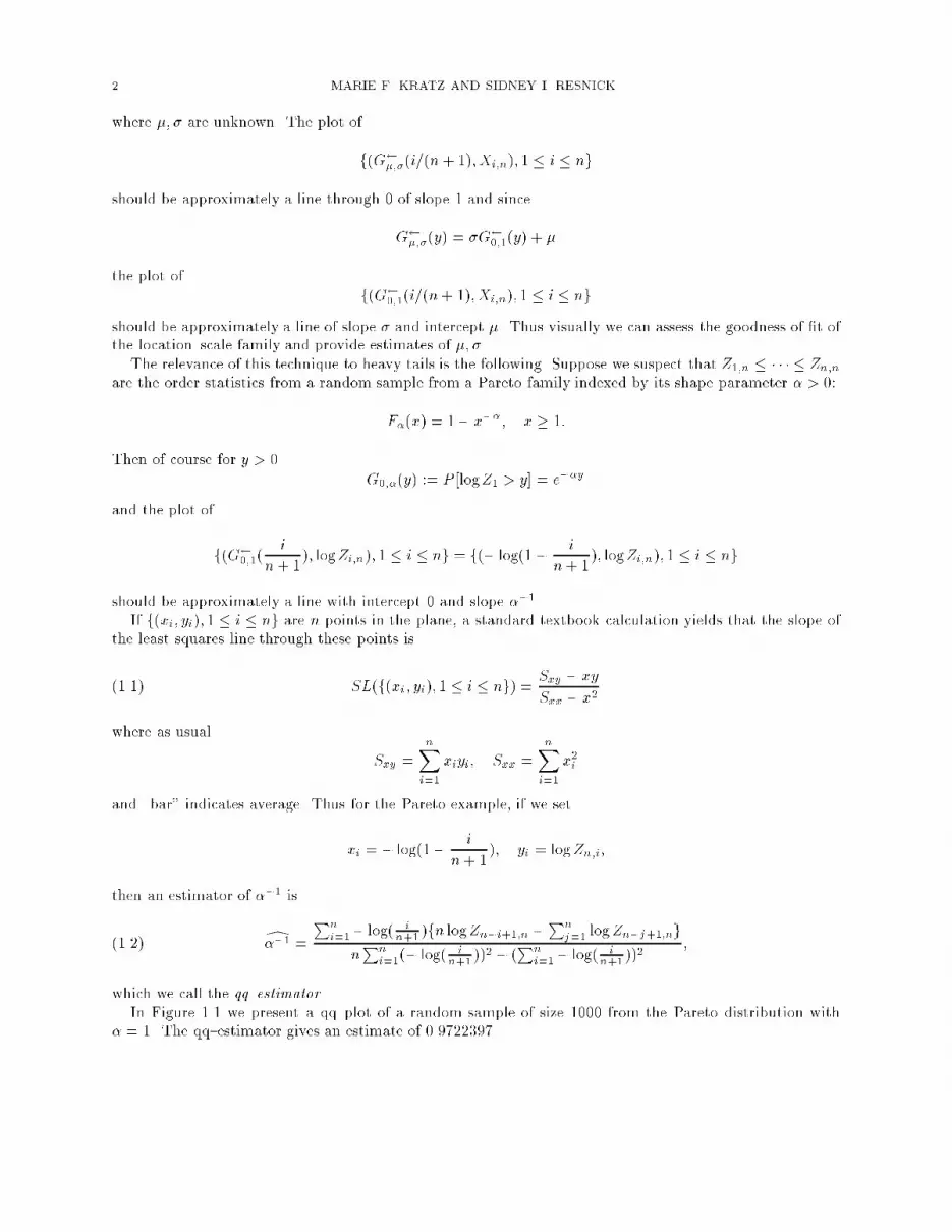
2 MARIE F. KRATZ AND SIDNEY I. RESNICKwhere �; � are unknown. The plot off(G �;�(i=(n + 1); Xi;n); 1 � i � ngshould be approximately a line through 0 of slope 1 and sinceG �;�(y) = �G 0;1(y) + �the plot of f(G 0;1(i=(n+ 1); Xi;n); 1 � i � ngshould be approximately a line of slope � and intercept �. Thus visually we can assess the goodness of �t ofthe location{scale family and provide estimates of �; �.The relevance of this technique to heavy tails is the following. Suppose we suspect that Z1;n � � � � � Zn;nare the order statistics from a random sample from a Pareto family indexed by its shape parameter � > 0:F�(x) = 1� x��; x � 1:Then of course for y > 0 G0;�(y) := P [logZ1 > y] = e��yand the plot off(G 0;1( in+ 1); logZi;n); 1 � i � ng = f(� log(1� in+ 1); logZi;n); 1 � i � ngshould be approximately a line with intercept 0 and slope ��1.If f(xi; yi); 1 � i � ng are n points in the plane, a standard textbook calculation yields that the slope ofthe least squares line through these points is(1.1) SL(f(xi; yi); 1 � i � ng) = �Sxy � �x�y�Sxx � �x2where as usual Sxy = nXi=1 xiyi; Sxx = nXi=1 x2iand \bar" indicates average. Thus for the Pareto example, if we setxi = � log(1� in+ 1); yi = logZn;i;then an estimator of ��1 is(1.2) d��1 = Pni=1� log( in+1 )fn logZn�i+1;n �Pnj=1 logZn�j+1;ngnPni=1(� log( in+1 ))2 � (Pni=1� log( in+1 ))2 ;which we call the qq{estimator .In Figure 1.1 we present a qq{plot of a random sample of size 1000 from the Pareto distribution with� = 1. The qq{estimator gives an estimate of 0.9722397.

THE QQ{{ESTIMATOR AND HEAVY TAILS 3••••••••••••••••••••••••••••••••••••••••••••••••••••••••••••••••••••••••
•••••••••••••••••••••••••••••••••••••••••••••••••••••••••••••••••••••••••••••••••••••••••••••••••••••••••••••••••••••••••••••••••••••
••••••••••••••••••••••••••••••••••••••••••••••••••••••••••••••••••••••••••••••••••••••••••••••••••••••••••••
••••••••••••••••••••••••••••••••••••••••••••••••••••••••••••••••••••••••••••••••••••••••••••••••••••••
••••••••••••••••••••••••••••••••••••••••••••••••••••••••••••••••••••••••••••••••••••••••••••
••••••••••••••••••••••••••••••••••••••••••••••••••••••••••••••••••••••
•••••••••••••••••••••••••••••••••••••••••••
••••••••••••••••••••••••••••••••••••••••••••
••••••••••••••••••••••••••
•••••••••••••••••
••••••••••••••••
••••••••••
•••••••
•••• •
• • • •
• • •
•
quantiles of exponential
log
sorte
d da
ta
0 2 4 6
02
46
Figure 1.1Because of the frequency with which the qq{plot is used, we sought to investigate the properties of the plotand the estimator when the underlying distribution was not exactly Pareto. If one wishes to drop the Paretoassumption but stay within the heavy tail class, one can assume the distribution is only Pareto from somepoint on (see, for example Feigin, Resnick and Starica (1994)) but we decided to make the more general andless ad-hoc assumption that tails were regularly varying. So we suppose we have a random sample Z1; : : : ; Znfrom a distribution F satisfying(1.3) 1� F (x) � x��L(x); (x!1)where L is a slowly varying function satisfyinglimt!1 L(tx)L(t) = 1:We now modify (1.2) to make it suitable for the regularly varying case. Here is the rationale for themodi�cation. Observe that since 1� F is regularly varying, we have for large t.(1.4) 1� F (tx)1� F (t) = P [Z1t > xjZ1 > t] � x��:Now choose k = k(n) ! 1 such that k=n ! 0. Then the k + 1st largest order statistic Zn�k;n satis�esZn�k;n P! 1 as n ! 1. This follows, for example, from Smirnov, (1952). Conditional on Zn�k;n we havethat Zn;n; Zn�1;n; : : : ; Zn�k+1;n have the distribution of the order statistics from a random sample of sizek from a distribution concentrating on (Zn�k;n;1) of the form F (�)=(1� F (Zn�k;n): Thus conditional onZn�k;n, �Zn�k+i;nZn�k;n ; i = 1; : : : ; k�behave like the order statistics from a sample of size k from the distribution concentrating on (1;1) withtail 1� F (Zn�k;nx)1� F (Zn�k;n) � x��

4 MARIE F. KRATZ AND SIDNEY I. RESNICKwhere the approximation follows from (1.4). So in the notation of (1.1) it is reasonable to de�ne the qq{estimator based on the upper k order statistics to be(1.5) d��1 = d��1(k) = SL(f(� log(1� ik + 1); log(Zn�k+i;nZn�k;n ); 1 � i � kg):Some modest simpli�cation of (1.4) is possible if we note the following readily checked properties of theSL function: For any real numbers a; b we have(1.6) SL(f(xi; yi); 1 � i � ng) = SL(f(xi + a; yi + b); 1 � i � ng):Thus (1.4) simpli�es to(1.7) d��1 = SL(f(� log(1 � ik + 1); logZn�k+i;n); 1 � i � kg):In practice we would make a qq{plot of all the data and choose k based on visual observation of theportion of the graph which looked linear. Then we would compute the slope of the line through the chosenupper k order statistics and the corresponding exponential quantiles. Choosing k is an art as well as ascience and the estimate of � is usually rather sensitive to the choice of k. Alternatively, one can plotf(k;d��1(k)); 1 � k � ng and look for a stable region of the graph as representing the true value of ��1.This is analogous to what is done with the Hill estimator of ��1(1.8) Hk;n = 1k kXi=1 log(Zn�k+i;nZn�k;n ):Choosing k is the Achilles heel of all these procedures; the di�culty can sometimes be lessened by smoothing.See Resnick and Starica (1995).In Section 2 we prove weak consistency of d��1 under the regular variation assumption (1.3). Section 3concentrates on proving asymptotic normality under a second order strengthening of (1.3). Section 4 containssome additional examples and comments.2. Consistency of the qq{estimator.In this Section we prove the weak consistency of the qq-estimator. In view of (1.5), (1.6) and (1.8) wemay write the estimator d��1 as(2.1) d��1 = 1kPki=1(� log(1� ik+1)) log(Zn�k+i;nZn�k;n )� 1k Pki=1(� log(1� ik+1))Hk1kPki=1(� log(1� ik+1))2 � ( 1kPki=1(� log(1� ik+1 ))2where the Hill estimator Hk was de�ned in (1.8).Theorem 2.1. Suppose k = k(n) ! 1 in such a way that as n ! 1 we have k=n ! 0. SupposeZ1; : : : ; Zn are a random sample from F , a distribution with regularly varying tail satisfying (1.3). Then theqq{estimator d��1 given in (2.1) is weakly consistent for 1=�:d��1 P! ��1as n!1.Proof. Write the denominator in (2.1) as 1kSxx � ( 1kSx)2
THE QQ{{ESTIMATOR AND HEAVY TAILS 5where as n!1 1kSxx =1k kXi=1(� log(1� ik + 1))2 � Z 10 (� logx)2dx= Z 10 y2e�ydy = 2(2.2)and 1kSx =1k kXi=1(� log(1� ik + 1)) � Z 10 (� logx)dx= Z 10 ye�ydy = 1:(2.3)Furthermore as n!1 1k kXi=1(� log(1� ik + 1))Hk � Z 10 (� logx)dxHk P! ��1by the weak consistency of the Hill estimator (Mason, 1982). So for consistency of the qq{estimator it su�cesto show(2.4) An := 1k kXi=1(� log(1� ik + 1)) log(Zn�k+i;nZn�k;n ) P! 2�:We do this by using Potter's inequalities (Bingham, Goldie and Teugels, 1986) and Renyi's representationof order statistics (Resnick, 1992, page 439). Potter's inequalities take the following form: Since 1=(1� F )is regularly varying with index �, the inverse U = (1=(1�F )) is regularly varying with index 1=� and for� > 0, there exists t0 = t0(�) such that if y � 1 and t � t0(2.5) (1� �)y��1�� � U (ty)U (t) � (1 + �)y��1+�:We now rephrase this in terms of the functionR = � log(1� F ) = logU :Then U = R � log and taking logarithms in (2.5) and then converting from a multiplicative to an additiveform yields that(2.6) log(1� �) + (��1 � �)y � logR (s+ y) � logR (s) � log(1 + �) + (��1 + �)yfor s � log t0; and y � 0.The reason for introducing the R function is that if E1; E2; : : :En are iid unit exponentially distributedrandom variables then (Z1; Z2; : : : ; Zn) d= (R (Ej); j = 1; : : : ; n):The Renyi representation (Resnick, 1992, Lemma 5.11.1) states that if E1;n � E2;n � � � � � En;n are theorder statistics associated to E1; E2; : : :En, then(2.7) (E1;n; E2;n� E1;n; : : : ; En;n� En�1;n) d= (Enn ; En�1n � 1 ; : : : ; En1 ):
6 MARIE F. KRATZ AND SIDNEY I. RESNICKFor An we haveAn =1k kXi=1(� log(1� ik + 1)) log(Zn�k+i;nZn�k;n )d=1k kXi=1(� log(1� ik + 1)) log(R (En�k+i;n)R (En�k;n) )= 1k kXi=1(� log(1� ik + 1)) (log(R (En�k;n + (En�k+i;n �En�k;n)) � logR (En�k;n))and applying the Potter inequality (2.6) we have the upper bound1k kXi=1(� log(1� ik + 1)) �log(1 + �) + (��1 + �)(En�k+i;n� En�k;n)�=(1 + o(1)) log(1 + �) + (��1 + �) 1k kXi=1(� log(1� ik + 1))(En�k+i;n � En�k;n);where we have applied (2.3). Of course a similar lower bound is obtained using the other half of the Potterinequalities. From the Renyi representation, for i = 1; : : : ; kEn�k+i;n �En�k;n = n�k+iXj=n�k+1(Ej;n �Ej�1;n)d= n�k+iXj=n�k+1 En�j+1n� j + 1= kXj=k�i+1 Ejj :Thus (2.4) will be proven provided we show(2.8) 1k kXi=1(� log( ik + 1)) kXj=i Ejj P! 2:For the proof of 2.8 we need two simple lemmas.Lemma 2.2. We have that(2.9) 1k kXj=1 log j = �1 + log k + 1kflogp2� + 12 logkg+ o(1):Proof of Lemma 2.2. From Stirling's formulak! � e�kkk+1=2p2�so that log k!� (�k + (k + 12) logk + logp2�)! 0:Since 1k logk! = 1k kXj=1 log j;the result follows. �

THE QQ{{ESTIMATOR AND HEAVY TAILS 7Lemma 2.3. If fEj; j � 1g are iid unit exponentially distributed random variables1k kXj=1Ej log j = op(1) + (�1 + logk + 1kflogp2� + 12 logkg:Proof of Lemma 2.3. By the classical Kolmogorov convergence criterion, the series1Xj=1 log jj (Ej � 1)converges a.s. since taking variances yields 1Xj=1� log jj �2 <1:Thus by Kronecker's Lemma (see, for example, Port, 1994)1k kXj=1(Ej � 1) log j ! 0almost surely as k !1. Thus 1k Pkj=1(Ej � 1) log j = op(1) and thus1k kXj=1Ej log j = op(1) + 1k kXj=1 log j:An appeal to Lemma 2.2 �nishes the proof. �Proof of (2.8). We now complete the proof of Theorem 2.1 by verifying (2.8). For what follows set�Ek = 1k kXj=1Ej:Then for (2.8) we have1k kXi=1(� log( ik + 1)) kXj=i Ejj=1k kXj=1 1j jXi=1(� log( ik + 1)!Ej=1k kXj=1 log(k + 1)� 1j jXi=1 log i!Ej= log(k + 1) �Ek � 1k kXj=1 1j jXi=1 log i!Ejand applying Lemma 2.2 we get

8 MARIE F. KRATZ AND SIDNEY I. RESNICK= log(k + 1) �Ek � 1k kXj=1��1 + log j +O( log jj )�Ej= log(k + 1) �Ek + �Ek � 1k kXj=1(log j)Ej � 1k kXj=1O( log jj )Ej:The last term on the right is op(1). Applying Lemma 2.3 we get= log(k + 1) �Ek + �Ek ��op(1)� 1 + log k +O( log kk �= log(k + 1) �Ek � log k + ( �Ek + 1) + op(1)=2 + log(k + 1) �Ek � logk + op(1):It remains to show that log(k + 1) �Ek � logk P! 0:This is easy since log(k + 1) �Ek � logk = log(k + 1)( �Ek � 1) + log(k + 1)� logk=log(k + 1)pk pk( �Ek � 1) + o(1)P!0;by the Central Limit Theorem. This completes the proof. �3. Asymptotic normality of the qq-estimator.We continue to suppose that fZn; n � 1g is iid with common distribution F such that 1� F is regularlyvarying at in�nity of order ��, with � > 0. Z1;n < Z2;n < : : : < Zn;n are the order statistics of Z1; : : : ; Zn.We investigate the limit distribution of the qq-estimator d��1 de�ned in (2.1). Because of (1.6) we can write(3.1) d��1 = kXi=1 � log� ik+1�8<:k log (Zn�i+1; n)� kXj=1 log (Zn�j+1; n)9=;k kXi=1 �� log� ik+1��2 � kXi=1 � log� ik+1�!2 :For this study, we will suppose that a second order regular variation condition holds for the non-decreasingfunction U , where recall U (t) = � 11� F � (t); t > 0:The condition is as follows. Set = ��1. We suppose there exists � � 0 and a function 0 < A(t)! 0 suchthat for all x > 1(3.2) U(tx)U(t) � x A(t) ! cx �x� � 1� � (t!1)for some c 2 R. If � = 0, interpret (x� � 1)=� as logx. Necessarily A(�) is regularly varying of index � andU is regularly varying of index . The form of the limit is discussed in de Haan and Stadm�uller (1994); see

THE QQ{{ESTIMATOR AND HEAVY TAILS 9also Geluk and de Haan (1987). By means of Vervaat's Lemma (Vervaat, 1972), (3.2) may be inverted andexpressed in terms of 1� F to obtain(3.3) 1�F (sx)1�F (s) � x��A� 11�F (s)� ! c�x���1� x��j�j � ;as s!1.As an example, suppose 1� F (x) = x�� + cx��1 ; x > 1where c > 0; �0 > � > 0: Then A(s) � ��1c(�0� � 1)s1��0=�; s!1and � = 1� �0� . As another example, consider the Cauchy distribution with densityF 0(x) = 1�(1 + x2) ; x 2 Rand distribution function F (x) = 12 + 1� arctanx; x 2 R:Then F (y) = tan (� (y � 1=2)) so U (x) = F (1 � 1=x) = cot(�=x) and from a power series expansion ofcot(z) we �nd U (x) = x� �1� �23x2 + 0� 1x2�� :This gives as t!1 U (tx)U (t) � x � x � 2�23t2 �1� x�22 �and with A(t) = 2�23t2we get U(tx)U(t) � xA(t) ! x�1� x�22 �so that � = �2 and � = = 1.We also need to assume a condition which restricts the growth of k = k(n). We assume(3.4) k!1; k=n! 0; pk A(n=k)! 0:Note this condition depends on the underlying (unknown) distribution F since the function A depends onF . This condition is commonly used in the literature. See for example Dekkers and de Haan (1989).We now state the result of this section.

10 MARIE F. KRATZ AND SIDNEY I. RESNICKTheorem 3.1. If (3.2) and (3.4) hold, then(3.5) pk �d��1 � ��1� d! N �0; 2��2� :Remark: The asymptotic variance of pk �d��1 � ��1� is thus 2��2. In contrast, the Hill estimatorHk;n = 1k k�1Xi=0 log�Zn�i; nZn�k;n� satis�es under (3.2) and (3.4)pk �Hk;n � ��1� d! N �0; ��2�and hence has an asymptotic variance of ��2. However, the Hill estimator exhibits considerable bias incertain circumstances and thus asymptotic variance is not a good criterion for superiority.Proof. We �rst use (3.2) to obtain inequalities. Following what has become a standard method, which isdescribed, for example, in lecture notes of de Haan (1991), we observe that since A(t)! 0, (3.2) impliesx� U (tx)U (t) � 1! 0as t!1 and hence log U (tx) � log U (t)� log xA(t) =log�x� U(tx)U(t) �A(t)=log�1 + �x� U(tx)U(t) � 1��A(t)�x� U(tx)U(t) � 1A(t) ! c�x� � 1� � :Thus V (t) := logU (t) � log t satis�esV (tx)� V (t)A(t) ! c�x� � 1� � :From Geluk and de Haan, 1987, page 16�, the convergence is locally uniform in x.Suppose for concreteness that c > 0 and � < 0. Then (Geluk and de Haan, 1987) V (1) = limt!1 V (t)exists and V (1)�V (t) � cj�j A(t) 2 RV�. Applying Potter's inequalities, given " > 0, there exists t0 = t0(")such that for t � t0 and x � 1(1� ")x��" � V (1)� V (tx)V (1)� V (t) � (1 + ")x�+"whence (1� ")x��" � 1 � V (t)� V (tx)V (1)� V (t) � (1 + ")x�+" � 1and so(3.6) �1� (1 + ")x�+"� c1A(t) � logU (tx)� logU (t)� logx � �1� (1� ")x��"� c2A(t):

THE QQ{{ESTIMATOR AND HEAVY TAILS 11where c2 = (1 + ")c=j�j and c1 = (1 � ")c=j�j. Similar inequalities hold if either c < 0 or � = 0 and weproceed with the proof assuming that (3.6) holds. Note that (3.6) can be rewritten in terms of F as(1� (1 + ")x�+")c1A(t) � logF �1� 1tx�� logF (1� 1t ) � logx� (1� (1� ")x��")c2A(t):(3.6')Recalling (2.1) and the notationSx = kXi=1 � log� ik + 1� and Sxx = kXi=1 �� log� ik + 1��2 ;we may write d��1 = 1k2 Pki=1� log� ik+1��i;kDwith �i;k = kXj=1 (logZn�i+1;n � logZn�j+1;n)and D = 1kSxx � �1kSx�2 ! 1; as n!1:In fact, we have that(3.7) pk d��1 � 1k2 kXi=1 � log� ik + 1��i;k! P! 0 (n!1):To see this, observe thatpk �����d��1 � 1k2 kXi=1 � log� ik + 1��i;k����� = pk ����1�DD ���� ����� 1k2 kXi=1 � log� ik + 1��i;k����� :From Section 2, k�2Pkj=1� log� ik+1��i;k is stochastically bounded and since D ! 1, (3.7) will be provedprovided we show(3.8) j1�D j = O� log2 kk � :We have1�D = 1� 1k kXi=1 log2 i+ 2 log(k + 1)k kXi=1 log i � log2(k + 1) + 1k 1k kXi=1 log i� log (k + 1)!2 :Since 1k Z k1 log2 udu � 1k kX1 log2 i � 1k Z k+11 log2 udu

12 MARIE F. KRATZ AND SIDNEY I. RESNICKand 1k Z k+1k (logu)2du � log2 kkand for x � 1 Z x1 log2 udu = 2(x� 1) + x logx(logx� 2);we �nd that(3.9) 1k kX1 log2 i = 2 + (log k) ((log k)� 2) +O� log2 kk � :The combination of (3.9) and Lemma 2.2 yield (3.8) and hence (3.7).Let U1; U2; : : : be independent uniform random variables on [0; 1] and let qn denote the left continuousuniform quantile function, de�ned by qn(t) = inffs : Fn(s) � tgwhere Fn is the uniform empirical distribution; that isqn(t) = � 0; for t = 0Ui;n; for i�1n < t � in and 1 � i � n:By using Zn�i+1;n d= F (Un�i+1;n) d= F (1� Ui;n);we have �i;k d= kXj=1 (logF (1� Ui;n) � logF (1� Uj;n)) = �j�i ��j<iwith �j�i := kXj=i(logF (1� Ui;n)� logF (1� Uj;n))and �j<i := i�1Xj=1 (logF (1 � Uj;n)� logF (1� Ui;n)) ;and by applying (3.6) to �j�i and �j<i, we get that for all " > 0, there exists t0 such that on the set[1=Uk;n > t0] (which, since Uk;n P! 0 is a set whose probability converges to 1)(3.10) Infi;k � �i;k � kXj=1 log�Uj;nUi;n� < Supi;kwhere Supi;k = kXj=i ( 1� (1� ")�Uj;nUi;n���"! c2A� 1Uj;n�)� i�1Xj=1( 1� (1 + ")�Ui;nUj;n��+"! c1A� 1Ui;n�)and

THE QQ{{ESTIMATOR AND HEAVY TAILS 13Infi;j = kXj=i ( 1� (1 + ")�Uj;nUi;n��+"! c1A� 1Uj;n�)� i�1Xj=1( 1� (1� ")�Ui;nUj;n���"! c2A� 1Ui;n�) :Therefore(3.11) �ik d= kXj=1 log�Uj;nUi;n�+ ei;k;ei;k being an error term such that Infi;k < ei;k < Supi;k. Because of (3.7) and (3.11) we thus haved��1 d= 1k2 kXi=1 � log� ik + 1��i;k + Op� 1pk�= 1�Dn + e(1)k + Op� 1pk� ;(3.12)where e(1)k := 1k2 kXi=1 � log� ik + 1� ei;kand Dn := 1k2 kXi=1 � log� ik + 1� kXj=1 log�Uj;nUi;n� :Now Dn = 1k2 k�1Xi=1 � log� i+ 1k + 1� k�1Xj=1 log�Uj+1;nUi+1;n�+ log(k + 1)k2 kXj=1 log�Uj;nU1;n�+ 1k2 kXi=2 � log� ik + 1� log�U1;nUi;n � :But log(k + 1)k2 kXj=1 log�Uj;nU1;n�+ 1k2 kXi=2 � log� ik + 1� log�U1;nUi;n � = 1k2 kXi=2 log i log�Ui;nU1;n� :We show(3.13) 1k2 kXi=2 log i log Ui;nU1;n = Op� 1pk� :

14 MARIE F. KRATZ AND SIDNEY I. RESNICKWe have 0 �pk 1k2 kXi=2 log i log Ui;nU1;n� log Uk;nU1;n pkk2 kXi=2 log i� log Uk;nU1;n � log kpk � = log�k � nkUk;nnU1;n � log kpk=(log k)2pk + log�nkUk;n� log kpk � lognU1;n log kpkP!0since nkUk;n P! 1 and fnU1;ng is convergent in distribution. We conclude that(3.14) Dn d= 1k2 k�1Xi=1 � log� i + 1k + 1� k�1Xj=1 log�Uj+1;nUi+1;n�+Op� 1pk� :But it is also true thatlog�Uj+1;nUi+1;n� d= log�1� Un�j;n1� Un�i;n�= log�1� qn(1� j=n)1� qn(1� i=n)�= log�1� qn(1� j=n)j=n �� log�1� qn(1� i=n)i=n �+ log�ji� :Moreover, by de�nition of the uniform quantile process, �n(t) = pn(qn(t) � t), we have, for 0 < s � 1log�1� qn(1� s)s � = log�1� (1� s)� n�1=2�n(1� s)s �= log�1� �n(1� s)spn �= � �n(1� s)spn +R(1)n (s):Then log�Uj+1;nUi+1;n� d= 1pn ��n(1 � i=n)i=n � �n(1� j=n)j=n �+ log�ji�+ R(2)n (i; j)with R(2)n (i; j) := R(1)n (j=n)� R(1)n (i=n)and by using the result of M. Cs�org}o, S. Cs�org}o, Horv�ath, and Mason (1986), namely �n(t) = �Bn(t) +n�1=2+�Op(t�) with 0 < � < 1=2, where fBn(s); 0 � s � 1g is a sequence of Brownian Bridges, we obtainlog�Uj+1;nUi+1;n� d= 1pn �Bn(1 � j=n)j=n � Bn(1� i=n)i=n �+ log�ji�+ R(3)n (i; j)

THE QQ{{ESTIMATOR AND HEAVY TAILS 15with R(3)n (i; j) := R(2)n (i; j) + 1n1�� �Op((i=n)�)i=n � Op((j=n)�)j=n � :This gives us(3.16) Dn d= �Mn + 1k2 k�1Xi=1 � log� i+ 1k + 1� k�1Xj=1 log(ji ) +R(4)nwith Mn := 1�k2pn k�1Xi=1 � log� i + 1k + 1� k�1Xj=1�Bn(1� j=n)j=n � Bn(1� i=n)i=n �and R(4)n := 1k2 k�1Xi=1 � log� i+ 1k + 1� k�1Xj=1R(3)n (i; j)but also R(4)n = Dn � 1k2 k�1Xi=1 � log� i + 1k + 1� k�1Xj=1 log�ji�� �Mn:Therefore, (3.12) and this last expression provided��1 =Mn + 1�k2 k�1Xi=1 � log� i + 1k + 1� k�1Xj=1 log�ji�+R(4)n + e(1)k=Mn + 1� + Rk + 1�R(4)n + e(1)kwith Rk = 1� 0@ 1k2 k�1Xi=1 � log� i+ 1k + 1� k�1Xj=1 log�ji�� 11A :To analyze Rk, we note1k2 k�1Xi=1 � log� i + 1k + 1� k�1Xj=1 log�ji�= 1k2 k�1Xi=1 � log� i+ 1k � k�1Xj=1 log�ji�= 1k2 k�1Xi=1 � log� i+ 1k � k�1Xj=1 log(j=k) + k � 1k2 k�1Xi=1 log� i+ 1k � log(i=k)� Z 12=k� logxdx Z 1� 1k1=k logxdx+ k � 1k Z 1� 1k1=k log�x+ 1k� logxdx=1 + O� log2 kk � :

16 MARIE F. KRATZ AND SIDNEY I. RESNICKThen Rk = ��1O((log2 k)=k) and pkRk = 0(1) as k!1. Finally, we get from (3.12), (3.14), (3.16)(3.17) ^��1 = ��1 +�n + En + 0p� 1pk�with(3.18) Mn := 1�k2pn k�1Xi=1 � log� i + 1k + 1� k�1Xj=1�Bn(1� j=n)j=n � Bn(1� i=n)i=n �and En = 1�R(4)n + e(1)k = En1 +En2;where from (3.16)En1 = 1�R(4)n = 1�k2 k�1Xi=1 � log� i + 1k + 1� k�1Xj=1�log�Uj+1;nUi+1;n�� log�ji�� �Mnand En2 = e(1)k is given after (3.12). We now analyze the behavior of each term in (3.17).Part 1 : Behavior of pkMn: RecallMn := 1�k2pn k�1Xi=1 � log� i+ 1k + 1� k�1Xj=1�Bn(1� j=n)j=n � Bn(1� i=n)i=n �= 1�k2pn k�1Xi=1 � log�i + 1k � k�1Xj=1�Bn(1� j=n)j=n � Bn(1� i=n)i=n � :By de�nition of the Brownian Bridge, Bn satis�es�Bn(1� t)t ; 0 < t � 1� d= �W (1)� W (t)t ; 0 < t � 1� ;where W is a standard Wiener process. SoMn d= 1�k2pn k�1Xi=1 � log� i + 1k � k�1Xj=1�W (j=n)j=n � W (i=n)i=n � :Since W (c�) d= pcW (�) for c > 0, we get by writingW (j=n)j=n = W ( jkk=n)j=k � k=n d= pk=nk=n W (j=k)j=k =pn=kW (j=k)j=kthat Mn d= 1�k2pk k�1Xi=1 � log�i + 1k � k�1Xj=1�W (j=k)j=k � W (i=k)i=k �

THE QQ{{ESTIMATOR AND HEAVY TAILS 17and thus pkMn d= 1� 1k k�1Xi=1 � log�i + 1k �!0@ 1k k�1Xj=1 W (j=k)j=k 1A� 1� �k � 1k � 1k k�1Xi=1 � log� i+ 1k � W (i=k)i=k! 1� �Z 10 � logudu��Z 10 W (s)s ds�� 1� Z 10 � loguW (u)u du= 1� �Z 10 W (s)s ds� Z 10 (� logu)W (u)u du�= 1� Z 10 (1 + logu)W (u)u du =: Z:So Z is a Gaussian random variable with mean 0 and varianceVarZ = 2�2 Z0<s<u<1(1 + logu)(1 + log s)s ^ uus duds = 2�2 ;the integral being performed via Mathematica. Thus we can conclude(3.19) pkMn d! N �0; 2=�2� :Part 2 : Behavior of pkEn :We will show that pkEn = Op(1) as k ! 1; n !1 and k=n ! 0. For this, we will split En into twoterms and use di�erent methods on each. Let En := En1 + En2, withEn1 := 1�k2 k�1Xi=1 � log� i + 1k + 1� k�1Xj=1 "log�Uj+1;nUi+1;n�� log�ji�� 1pn Bn(1� jn )jn � Bn(1� in )in !#and En2 := 1�k2 kXi=1 � log� ik + 1� ei;k;where Infi;k < ei;k < supi;k:We �rst consider En1 and follow the method developed in Cs�org}o, Deheuvels and Mason (1985). We haveEn1 = 1�k k�1Xi=1 � log�i + 1k �Ri;kwhere Ri;k := 1k k�1Xj=1�log�Uj+1;nUi+1;n�� log (j=i) � 1pn �Bn(1� j=n)j=n � Bn(1� i=n)i=n �� :
18 MARIE F. KRATZ AND SIDNEY I. RESNICKUsing again (3.15), we getRi;k d=1k k�1Xj=1��log�1� qn(1� j=n)j=n �� 1pn Bn(1� j=n)j=n ���log�1� qn(1� i=n)i=n �� 1pn Bn(1� i=n)i=n ��and then En1 = 1�k k�1Xi=1 � log� i+ 1k � 1k k�1Xj=1�log�1� qn(1� j=n)j=n �� 1pn Bn(1� j=n)j=n �� 1�k k�1Xi=1 � log� i+ 1k ��log�1� qn(1� i=n)i=n �� 1pn Bn(1� i=n)i=n � :De�ne ck = k�1 k�1Xi=1 � log� i+ 1k �so that ck ! 1 and�En1 = 1k k�1Xi=1 �ck � log� i+ 1k ��"log 1� qn(1� in)i=n !� 1pn Bn(1� in)i=n # :Write log 1� qn(1� in )in ! = log 1� �n(1� in )inpn !=��n(1� in)inpn + g �n(1� in)inpn !where g(u) = u+ log(1� u): So� jEn1j <=1k k�1Xi=1 �c(k) � log�i + 1k �� �������n(1� in) �Bn(1� in)inpn �����+ 1k k�1Xi=1 �c(k)� log� i+ 1k �� �����g �n(1� in )inpn !�����= jE0n1j+ jE00n1j :From Lemma 10 of Cs�org}o, Deheuvels and Mason (1985), we have for 0 < � < 1=2sup1n+1���1 ������(1 � �)� Bn(1� �)���+1=2 ���� = Op �n��� :

THE QQ{{ESTIMATOR AND HEAVY TAILS 19Thus jE0n1j �1k k�1Xi=1 �2� log� i+ 1k ���������n(1� in )� Bn(1� in )( in)��+1=2 ����� � in���+1=2 = inpn�Op(n��)n�� 1k k�1Xi=1 �2� log�i + 1k ��� ik����1=2 k���1=2=Op(1)k���1=2 Z 10 (2� logu)u���1=2du=Op(k���1=2):Therefore pkE0n1 = O�(k��) d! 0:For E00n1 we have thatg �n(1� in )inpn ! = log 1� qn(1� in )i=n !+ �n(1� in )inpn= log 1� qn(1� in )i=n !+ qn(1� in )� (1� in )i=n= log� in +�1� in � qn�1� in���� log in + qn�1� in�� �1� in�and from a two-term Taylor expansion, this is= � �1� in � qn �1� in��22�2n � in� = ��2n �1� in�2n�2n � in�where min� in ; 1� qn�1� in�� � �n� in� � max� in ; 1� qn�1� in�� :From Lemma 13, page 1069 of Cs�org}o, Deheuvels and Mason (1985), we obtain the following: given " > 0,there exists n0 and � > 1 such that n � n0 impliesP (An(�)) > 1� "where An(�) = \1n+1���1��� � 1� qn(1 � �) � ��� :Thus on An(�) we observe that for n � n0i�n � in ^ i�n � �n� in� � in _ �� in� = � in :

20 MARIE F. KRATZ AND SIDNEY I. RESNICKTherefore on An(�) jE00n1j =1k k�1Xi=1 �c(k)� log� i + 1k �� �����g �n(1� in )inpn !������1k k�1Xi=1 �c(k)� log� i + 1k �� �2n(1� in)2n�2n( in)�1k k�1Xi=1 �2� log� i+ 1k ���2 �2n(1� in )2n � in�2 :It follows that for any � > 0P hpk jE00n1j >i �P (An(�)c) + P "pkk k�1Xi=1 �(2� log�i + 1k ���2 �2n(1� in2n( in)2 > �#�" + P "pkk k�1Xi=1 �2� log�i + 1k ���2 �2n(1� in2n( in)2 > �# :Now from Lemma 14, page 1070 of Cs�org}o, Deheuvels and Mason (1985), for every � 2 (0; 12 ) we havesup1n���1 �����n(1� �)pn�1�� ���� = Op �n��� :Pick �" �14 ; 12� and thenP hpk jE00n1j > �i �"+ P "�2pk 1k k�1Xi=1 �2� log� i+ 1k �� �2n �1� in�n � in�2(1��) � in�2(1��)� in�2 > �#="+ P "Op(1)k�2�pk 1k k�1Xi=1 �2� log� i+ 1k ��� ik��2� > �#="+ � hOp �k�2�+1=2� > �i :Since �2� + 12 < 0, as a consequence of � > 14 , and since " > 0 is arbitrary, we getpk jE00n1j P! 0as desired.We now consider the remainder En2 using properties of regular variation. Recall that(3.21) 1�k2 kXi=1 � log� ik � 1� Infi;k < En2 < 1�k2 kXi=1 � log� ik + 1�Supi;k:and consider the upper bound Bk of En2. We prove that pkBk P! 0 as k!1. Let Bk := 1� �B(1)k + B(2)k �,with B(1)k := 1k2 kXi=1 � log� ik + 1� kXj=i 1� (1� ")�Uj;nUi;n���"! c2A� 1Uj;n�and
THE QQ{{ESTIMATOR AND HEAVY TAILS 21B(2)k := 1k2 kXi=1 log� ik + 1� i�1Xj=1 1� (1 + ")�Ui;nUj;n��+"! c1A� 1Ui;n� :We �rst show pkB(2)k P! 0. By Potter's inequalities (Bingham, Goldie, Teugels, 1987), for given " > 0,there exists t0 such that for t � t0 and all x � 1(1� �)x��" � A(tx)A(t) � (1 + �)x�+":Therefore for i = 1; : : : ; k A� 1Ui;n� =A� 1Uk+1;n � Uk+1;nUi;n ���Uk+1;nUi;n ��+� A� 1Uk+1;n�on the set �Uk+1;n � t�10 �, which is a set whose probability approaches 1 as n!1. So it su�ces to provepk 1k2 kXi=1 ����log ik + 1���� i�1Xj=1 �����1� (1 + ")�Ui;nUj;n��+"�����A� 1Ui;n�=pkA� 1Uk+1;n� 1k2 kXi=1 � log ik + 1 i�1Xj=1 �����1 + (1 + ")�Ui;nUj;n��+"����� �Uk+1;nUi;n ��+" P! 0:Now Uk+1;n= kn P! 1 implies by regular variation that A� 1Uk;n� =A(n=k) P! 1 so since pkA(n=k) ! 0 isassumed in (3.4), it remains to show that1k kXi=1 � log ik + 1 �Uk+1;nUi;n ��+" + 1k2 kXi=1 � log ik + 1 i�1Xj=1�Uk+1;nUj;n ��+" = A +Bis stochastically bounded. Set �i = E1+ � � �+Ei; i � 1 where fEn; n � 1g is iid with P [E1 > x] = e�x; x > 0.Then (U1;n; � � � ; Unn) d= � �1�n+1 ; � � � ; �n�n+1� :Thus A has the same distribution as 1k kXi=1 �� log ik + 1���k+1�i ��+" :Since �i � i a.s. as i ! 1, it is now clear that A is stochastically bounded. B is handled similarly afterobserving that B � 1k kXi=1 � log ik + 1!0@1k kXj=1�Uk+1;nUj;n �1A�+"d= 1k kXi=1 � log� ik + 1�!0@ 1k kXj=1 1(�j j�k)�+ "1A

22 MARIE F. KRATZ AND SIDNEY I. RESNICKand 1k kXi=1 � log� ik + 1� � Z 10 � loguduand 1k kXj=1 1(�j j�k)�+" � (const) 1k kXj=1 1(j=k)�+" � const Z 10 u�(�+")du <1:We now deal with B(1)k . Again, using Potter's inequalities we getA� 1Uj;n� =A� 1Uk;n � Uk;nUj;n ��A(1=Uk;n)�Uk;nUj;n��+" (1 + ")on [Uk;n � t0]. Also A(1=Uk;n)=A(n=k) P! 1. So to show pkB(1)k P! 0 it su�ces to show(3.23) 1k2 kXi=1 � log� ik + 1� kXj=i �Uk;nUj;n��+"is stochastically bounded. The expression in (3.23) is bounded above by 1k kXi=1 � log ik + 1!0@ 1k kXj=1�Uk;nUj;n��+"1Ad=(1 + o(1)) 1k kXj=1� 1�j=�k��+"which is stochastically bounded as checked when dealing with B of B(2)k . 194z So we can conclude thatpkBk P! 0 as k ! 1. Of course, we proceed in exactly the same way for the lower bound of En2. Thosetwo results on the upper and lower bounds imply that pkEn2 P! 0 as k!1, which completes the proof ofpkEn = 0p(1) as k!1. �4. Concluding remarks and examples.The qq estimator is easy to implement and we give some examples of its use. Write �̂(k) for 1=d��1 whenk upper order statistics are used in the estimation of �. We then make a plot of f(k; �̂(k)); 1 � k � ng andcompare it with the corresponding Hill plot f(k;H�1k;n); 1 � k � ng.Figure 1 is a simple comparison of the Hill plot and the qq{plot of estimates of � for 1000 observationsfrom a Pareto distribution where � = 1: Examining the qq{plot shows an estimate of about .98. The qq{plotseems to be a bit less volatile than the Hill plot.

THE QQ{{ESTIMATOR AND HEAVY TAILS 23number of order statistics
Hill e
stimate
of al
pha
0 200 400 600 800 1000
0.60.8
1.01.2
0 200 400 600 800 1000
0.50.6
0.70.8
0.91.0
number of order statistics
qq-es
timate
of al
phaFigure 4.1Next, we consider an example of a set of real data which exhibits large values and seems to be generated bya sequence of independent random variables. The data set represents the interarrival times between packetsgenerated and sent to a host by a terminal during a logged-on session. The terminal hooks to a networkthrough a host and communicates with the network sending and receiving packets. The length of the periodsbetween two consecutive packets received by the host were recorded as our data. The total length of thedata is 783. Figure 4.2 is a time series plot of our data set showing indications of heavy tails.
0 200 400 600 800
020
040
060
080
0
Packets
Figure 4.2To assess the appropriateness of applying either the Hill estimator or the qq{estimator, both of whichare designed for independent data, we next examine the classical acf function and a modi�cation called theheavy tailed acf: �HEAV (h) = Pn�hi=1 ZiZi+hPni=1 Z2i :The classical acf function applies a mean correction which is not be appropriate in the heavy tailed case.Plots which vary little from 0 are exploratory evidence of independence; as seen in Figure 4.3, this is thecase with this data.

24 MARIE F. KRATZ AND SIDNEY I. RESNICKLag
ACF
0 5 10 15 20 25
0.00.2
0.40.6
0.81.0
Series : Packets
Lag
heav
y tail
acf
0 5 10 15 20 25 30
-1.0
-0.5
0.00.5
1.0
Series : Packets
Figure 4.3Finally, in Figure 4.4 we display the Hill and qq plots. The Hill plot is somewhat inconclusive. Theqq{plot indicates a value of about .97 A smoothed version of the Hill plot (Resnick and Starica (1995))yields a value of about 1.1.number of order statistics
Hill e
stimate
of al
pha
0 200 400 600 800
0.20.4
0.60.8
1.0
0 200 400 600 800
0.50.6
0.70.8
0.9
number of order statistics
qq-es
timate
of al
phaFigure 4.4The Hill estimator, being optimized for the Pareto distribution, is likely to exhibit considerable bias whenthe distribution has a regularly varying tail. Consider 5000 observations from the distribution F with tail(4.1) 1� F (x) � x�1(logx)5:The logarithm in the tail fools both estimators as shown in Figure 4.5. Remember the correct answer is 1.
number of order statistics
Hill e
stimate
of al
pha
0 1000 2000 3000 4000 5000
0.00.5
1.01.5
2.02.5
0 1000 2000 3000 4000 5000
0.20.4
0.60.8
1.01.2
1.41.6
number of order statistics
qq-es
timate
of al
phaFigure 4.5

THE QQ{{ESTIMATOR AND HEAVY TAILS 25Our last plot, Figure 4.6, continues to consider the data from the tail in (4.1) and exhibits a static qq{plotfor a �xed value of k, namely k = 500. The plot shows many upper order statistics of the log sorted datadeviating signi�cantly from the least squares line plotted through the upper 500 log sorted order statistics.One of the advantages of qq{plotting over the Hill estimator is that the residuals contain information whichpotentially can be utilized to combat the bias in the estimates when the tail is not Pareto. We hope in thenear future to develop this into a technique which will be useful in bias correction.••••••••••••••••••••••••••••••••••••••••••••••••••••••••••••••••••••••••••••••••••••••••••••••••••••••••••••••••••••••••••••••••••••••••••••••••••••••••••••••••••••••••••••••••••••••••••••••••••••••••••••••••••••••••••••••••••••••••••••••••••••••••••••••••••••••••••••
••••••••••••••••••••••••••••••••••••••••••••••••••••••••••••••
••••••••••••••••••••••••••••••••••
•••••••••••••••••••••••••
•••••••••••••••••••
•••••••••••••••••••
•••••••••••••
•••••••••••••
•••••••••
•••••
••••• • • • • • • • • • •
•
quantiles of exponential
log so
rted d
ata
3 4 5 6 7 8
810
1214
16
Figure 4.6ReferencesBingham,N., Goldie, C. and Teugels, J., Regular Variation, Encyclopedia of Mathematics and its Applications, CambridgeUniversity Press, Cambridge, UK, 1987.Castillo, E., Extreme Value Theory in Engineering, Academic Press, San Diego, California, 1988.Cs�org}o, M., Cs�org}o, S., Horv�ath, L. and Mason, D., Weighted Empirical and quantile processes, Ann. Probability 14 (1986),31-85.Cs�org}o, S., Deheuvels, P. and Mason D., Kernel Estimates of the tail index of a distribution, Ann. Statist. 13 (1985),1050{1077.Dekkers, A. and Haan, L. de, On the estimation of the extreme value index and large quantile estimation, Ann. Statist. 17(1989), 1795{1832.Feigin, Paul D., Resnick, Sidney I. and St�aric�a, C�at�alin, Testing for Independence in Heavy Tailed and Positive InnovationTime Series, Submitted (1994).Haan, L. de, Extreme Value Statistics, Lecture Notes, Econometric Institute, Erasmus University, Rotterdam (1991).Geluk, J. and Haan, L. de, Regular Variation, Extensions and Tauberian Theorems, CWI Tract 40, Center for Mathematicsand Computer Science, P.O. Box 4079, 1009 AB Amsterdam, The Netherlands, 1987.Haan, L. de and Stadtm�uller, U., Generalized regular variation of second order, Preprint.Mason, D., Laws of large numbers for sums of extreme values, Ann. Probability 10 (1982), 754{764.Port, Sidney, Theoretical Probability for Applications, John Wiley & Sons, New York, 1994.Resnick, S., Adventures in Stochastic Processes, Birkhauser, Boston, 1992.Resnick, Sidney and St�aric�a, C�at�alin, Smoothing the Hill estimator, Preprint (1995).Rice, J., Mathematical Statistics and Data Analysis, Brooks/Cole Publishing, Paci�c Grove, Cali�fornia, 1988.Smirnov, N.V., Limit distributions for the terms of a variational series, Amer. Math. Soc. Transl. Ser. I 11 (1952), 82{143.Vervaat, W., Functional central limit theorems for processes with positive drift and their inverses, Z. Wahrscheinlichkeits-theory verw. Geb. 23 (1972), 249-253.Marie Kratz, Universit�e Ren�e Descartes, Paris V U.F.R. de Math�ematiques et Informatique 45, rue des Saints-P�eres 75270 Paris Cedex 06, FranceE-mail: [email protected] I. Resnick, Cornell University, School of Operations Research and Industrial Engineering, ETC Build-ing, Ithaca, NY 14853 USAE-mail: [email protected]