Unresolved Issues in Weighting Survey Data

Unresolved Issues in Weighting Survey Data

Peter Lynn ISER, University of Essex, UK

Roadmap of the Presentation

• Introduction/Background

- Reasons for weighting

- Types of weighting

- Requirements for successful weighting

• Problems/Issues in implementing successful weighting

- Unknown selection probabilities

- Uncertainty regarding eligibility

- Lack of (good) covariates

- Variation in mean response propensity for overlapping groups

- Variation between groups in predictors of response

• Possible solutions / current research

Lynn | ABS ASB, 21 October 2013

1. Reasons for Weighting

To improve statistical accuracy by adjusting for ways in which the

sample structure/composition may not match that of the

population, due to:

• Variations in selection probability;

• Random sampling variance;

• Variations in response (participation) probability.

For consistency between series / surveys (“coherence”)

For cosmetic reasons


2. Types of Weighting

• Design weighting:

𝑤𝑖𝐷 = 1

𝑃𝑖𝑆

• Non-response weighting:

𝑤𝑖𝑅 = 1

𝑃𝑖𝑅

• Post-stratification:

𝑤ℎ𝑖𝑃 =

𝛱ℎ𝜋ℎ

𝑤ℎ𝑒𝑟𝑒 𝜋ℎ = 𝑤𝑖

𝐷𝑤𝑖𝑅𝐼ℎ

𝑖=1

𝑤𝑖𝐷𝑤𝑖

𝑅𝐼ℎ𝑖=1

𝐻ℎ=1


i = element; h = post-stratum

Why Does Weighting Matter?

Case Study: Understanding Society wave 1

Estimates of means, proportions and regression coefficients:

•Unweighted

•Design-weighted

•Design-weighted with non-response adjustment and post-

stratification



No weights Design Design+NR n

% Male 44.1 43.8 48.9 47,061




% Male 44.1 43.8 48.9 47,061

% “Religion makes a great

difference to life”

22.2 16.5 17.0 46,924




% Male 44.1 43.8 48.9 47,061



22.2 16.5 17.0 46,924

Usual monthly pay (mean) 1817.4 1844.6 1896.6 22,524

95% C.I. (1793,1842) (1819,1870) (1867,1925)




% Male 44.1 43.8 48.9 47,061



22.2 16.5 17.0 46,924


95% C.I. (1793,1842) (1819,1870) (1867,1925)

Constant 2269.9 2350.5 2330.8

Female (p) -820.1 (.00) -903.6 (.00) -881.8 (.00)




% Male 44.1 43.8 48.9 47,061



22.2 16.5 17.0 46,924


95% C.I. (1793,1842) (1819,1870) (1867,1925)

Constant 2269.9 2350.5 2330.8

Female (p) -820.1 (.00) -903.6 (.00) -881.8 (.00)

Constant 1823.8 1834.4 1887.5

Non-UK-born (p) -36.3 (.28) +93.0 (.01) +73.1 (.08)




% Male 44.1 43.8 48.9 47,061



22.2 16.5 17.0 46,924


95% C.I. (1793,1842) (1819,1870) (1867,1925)

Constant 2269.9 2350.5 2330.8

Female (p) -820.1 (.00) -903.6 (.00) -881.8 (.00)

Constant 1823.8 1834.4 1887.5

Non-UK-born (p) -36.3 (.28) +93.0 (.01) +73.1 (.08)

Constant 1833.9 1850.4 1904.3

Post-2000 immigrant (p) -217.8 (.00) -118.8 (.02) -135.6 (.02)


2.1 Design Weighting

Requirement: Known selection probability for every sampled unit

Issue: Sometimes selection probability is unknown (even though it

is in principle tractable, unlike non-probability designs)

• Examples:

- 1. Single frame with duplicates

- 2. Multiple frame sampling (at one point in time)

- 3. Sampling at multiple points in time

Solution: Typically involves adding questions to the survey, the

answers to which can be used to approximate the selection

probability


Example 1: Duplicates

Survey of motorcycle riders for UK Dept of Transport

Frame of registered motorcycles:

- multiple motorcycles can be registered to same person

- not possible to identify duplicates in advance of sample selection

Solution:

- select motorcycles with equal probabilities;

- identify “main rider” of each sampled motorcycle;

- ask each respondent how many registered motorcycles they are

main rider of


Example 2: Multiple Frames


Dual-frame sampling common in telephone surveys;

A method to deal with coverage error;

Persons may have multiple chances of selection from same frame

(like example 1);

But they may also have a chance of selection from the other frame

Landline

phones

Cell

phones

Example 2: Multiple Frames

Solution:

- Ask (for landlines) how many people in the household, ni , (and

make random selection);

- Ask how many other landlines connect to this household, mi

- Ask how many cell phones selected person has, ci

- Estimate

Note assumptions:

- all household members use all landlines

- cell phones only used by one person


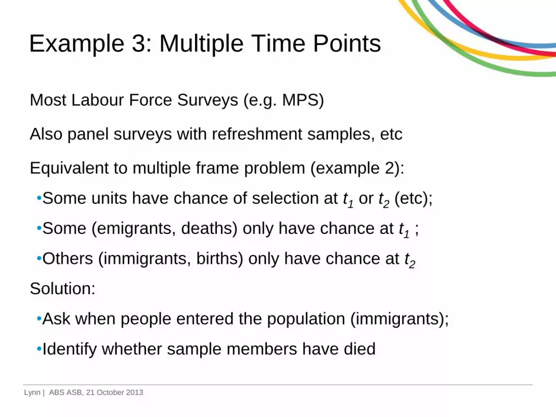
Example 3: Multiple Time Points

Most Labour Force Surveys (e.g. MPS)

Also panel surveys with refreshment samples, etc

Equivalent to multiple frame problem (example 2):

•Some units have chance of selection at t1 or t2 (etc);

•Some (emigrants, deaths) only have chance at t1 ;

•Others (immigrants, births) only have chance at t2

Solution:

•Ask when people entered the population (immigrants);

•Identify whether sample members have died


2.2 Non-Response Weighting

Requirement: To know for each sampled unit

• Eligibility;

• Response outcome;

• A set of covariates that should correlate both with survey

variables and with response propensity

This allows us to model response propensity and hence obtain

The model may be adjustment cells (implicit model) or, more

commonly, logistic regression, segmentation model etc.

may be model prediction, mean model prediction within cell,

observed response rate within cell


Non-Response Weighting ctd.

Issues:

• Eligibility may not always be known;

• Covariates (or good ones) may not be available

• Response propensity may depend on frame or time point (as in

examples 2 and 3 above)

• Relevant covariates may differ between analytically-import

subgroups


2.2.1 Unknown Eligibility

Examples:

• Screening for a subpopulation, e.g. ethnic minorities, people with

disabilities, families with young children

• Panel surveys, in which sample members can become ineligible

over time (e.g. die, emigrate, leave residential population)

For some non-respondents, eligibility will not be known


Unknown Eligibility

Solutions:

• Typically, eligibility status (binary) is imputed for each sampled

unit of uncertain eligibility, e.g. based on outcome code, record

linkage, predictive matching, survival analysis based on number of

attempts, etc

• Error-prone, and errors are often likely to be systematic

• Kaminska & Lynn (2012) propose an alternative that involves

predicting a probability of eligibility and using this as a weight in

the non-response model


Predicting the Probability of Eligibility

Steps:

• Using only units of known eligibility, fit model predicting eligibility;

• The models uses only covariates available for all sample units;

• Apply the model to the units of unknown eligibility, thus obtaining

predicted values in the range (0, 1)

• New variable, “eligibility probability” equals 1 for units known to

be eligible, 0 for units known to be ineligible, and model-predicted

probability for units of unknown eligibility

• This variable is then used as a weight in the model of non-

response propensity


Case Study I

Understanding Society: UK Household Longitudinal Study

Wave 1 boost sample of ethnic minorities via address screening

Model of eligibility excluded categories of ineligibility that should

always be identified (e.g. not yet built, non-residential): based on

other known ineligibles plus all known eligibles

Covariates were sample month, region, ethnic minority population

density (from Census), and various neighbourhood characteristics

from administrative data


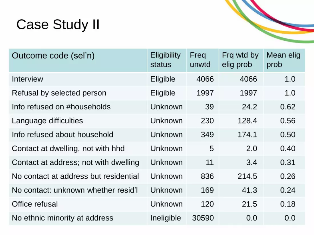
Case Study II


Outcome code (sel’n) Eligibility

status

Freq

unwtd

Frq wtd by

elig prob

Mean elig

prob

Interview Eligible 4066 4066 1.0

Refusal by selected person Eligible 1997 1997 1.0

Info refused on #households Unknown 39 24.2 0.62

Language difficulties Unknown 230 128.4 0.56

Info refused about household Unknown 349 174.1 0.50

Contact at dwelling, not with hhd Unknown 5 2.0 0.40

Contact at address; not with dwelling Unknown 11 3.4 0.31

No contact at address but residential Unknown 836 214.5 0.26

No contact: unknown whether resid’l Unknown 169 41.3 0.24

Office refusal Unknown 120 21.5 0.18

No ethnic minority at address Ineligible 30590 0.0 0.0

2.2.2 Covariates

Efforts can be made to obtain these by various means:

• From sampling frame (e.g. business register or popul’n register);

• Through record linkage;

• Through geographical linkage or other higher-level unit;

• Through interviewer observation (face-to-face surveys);

• Survey paradata (recent conferences, courses, book by Kreuter

et al, special issue of JRSSA)


2.2.3 Response Propensity Dependent on Frame or Time Point

Examples:

• Dual-frame (example 1 above): same individual may be less

likely to respond on cell phone than on landline;

• Multiple time points: responding at fourth wave is less probable

than responding at first wave (etc)

Methods that assume response propensity to be independent of

frame / time point may introduce systematic error


Dependent Response Propensity

Current approaches:

• Post-stratification: first design-weight the total sample, then post-

stratify to population;

• Non-response adjustment for each frame separately, then apply

design weights.

Both rely on equivalent assumption that, for units with multiple

selection chances (e.g. people with both a landline and cell

phone), response propensity is independent of which chance was

realised (i.e. which frame they were sampled from, or at which

time point they were sampled)

Kaminska & Lynn (2013) propose an approach that is free from

this assumption


Illustration: Dual-Frame


1. Landline

phones

2. Cell

phones A C B

kAp 1 kBp 2kCkC pp 21

i - part of sample (A,B,C)

j – sampling frame (1,2)

k – respondent

ijkp - selection probability

Nonresponse


1. Landline

phones

2. Cell

phones A C B

kAkA rp 11 kBkB rp 22

kCkCkCkC

kCkC

kCkC

rprp

rp

rp

2211

22

11

i - part of sample (A,B,C)

j – sampling frame (1,2)

k – respondent

ijkr - response probability

Method

Estimate:

Allowing

• we observe response only once

• and we have predictors for each frame only

• How do we estimate (response probability if

selected through landline) for people who were selected

through cell phone?


krr kCkC 21 ,

kCr 1

kCkC rr 21

Double Prediction

• Step 1:

where x are predictors for frame 1

• Step 2: save out

• Step 3:

where x’ are predictors for respondents (from

questionnaire)

• Step 4: infer to those selected through frame

2 using common predictors x’

• Step 5: repeat steps 1-4 for


xr kC )log( 1

kCr 1'

''' 1 xr kC

kCr 1"

kCr 2

2.2.4 Predictors Differ between Subgroups

Any model with only main effects assumes predictors do not vary

between subgroups

Issues:

• If weighting does not take this into account, subgroup estimation

will be sub-optimal (systematic error possible)

• Can produce a weight based on separate models for subgroups

only if the subgroups are mutually exclusive and comprehensive


Predictors Differ between Subgroups

Examples:

• Demographic subgroups, e.g. analysis of retired persons, with

weights developed for all responding adults

• Combinations of waves in a panel survey, e.g. analysis that uses

only data collected in waves 1, 4 and 7, with weights developed

for those who responded in all of waves 1 to 8 (balanced panel)

• Combinations of survey instruments, e.g. analysis of persons

who responded to main interview and self-completion follow-up,

with weights developed for all main interview respondents



Possible solutions:

• Cell weighting, with cells defined by interactions (but still requires

the relevant interactions to first be identified);

• Segmentation modelling (better - systematic identification of

interactions – but other disadvantages);

• Model with explicit interaction terms (but can get too complex);

• Separate estimation for subgroups (optimal for all examples, but

considerable extra analysis work)



Current research:

• Sadig (2014a): Separate estimation for analytically-interesting

combinations of waves in a panel survey: effects on estimates

based on specific wave combinations;

• Sadig (2014b): Separate estimation for age groups: effects on

age-related analysis (e.g. health) both specific age groups and for

total population


Final Words

Adjustment for structural differences between sample and

population are important: estimates can otherwise be biased

Weighting is an effective way to make these adjustments

Some aspects of weighting are straightforward and uncontroversial

Some methods are widely accepted despite undesirable properties

Some methods require research and development


Thank you!

Peter Lynn

ISER, University of Essex, UK

[email protected]

www.iser.essex.ac.uk

www.understandingsociety.ac.uk

Appendix

Extra Material


Current approach 1: post-stratification


Method: take design weighted sample and

post-stratify it to external

benchmarks

Landline

phones Cell

phones A C B

For part C:

Assumption:

kkA rp ..1 kkB rp ..2kkCkC rpp ..21 )(

kkCkC rpp ..21 )(

kkCkC rrr ..21

Current approach 2: nonresponse correction for each frame separately


Method:

• use IVs for landline phones and

correct for nonresponse for those

selected through landline

• same for cell phone

• put them together with correct

design weights

1. Landline

phones 2. Cell

phones

A B

For part C:

kAkA rp 11 kBkB rp 22

kkCkC rrr 1.21

kAkA rp 11 - if selected through frame 1

- if selected through frame 2 kBkB rp 22

& kkCkC rrr 2.21 Assumption:

kkCkC rrr ..21

Double prediction

• Step 1: predict for

everyone selected through frame 1

using predictors from frame 1.

• Step 2: Save estimated

from the model.

• Step 3: predict estimated

using predictors available for all respondents

(from questionnaire)

• Step 4: Infer to those selected

through frame 2


kCr 1

kCr 1

kCr 1

kCr 1

kCr 1

Com

mon p

redic

tors

kCr 1"

kCr 1'

Frame 1

Frame 2

Application (Understanding Society, UK)

1991 Original

Sample

1999 Sc and

W boost

2001 NI

sample

2009

UKHLS

sample

If only correction for selection

probabilities:

Assumption that attrition over 18 years is

the same as attrition over 2 years

Documents

Unresolved Issues in Weighting Survey Data