Unrestricted vs Restricted Cut in a TableauMethod for Boolean Circuits?

Matti Jarvisalo, Tommi Junttila, and Ilkka Niemela

Laboratory for Theoretical Computer ScienceHelsinki University of Technology

P.O. Box 5400, FI-02015 TKK, Finlandmatti.jarvisalo,tommi.junttila,ilkka.niemela@tkk.fi

Abstract. This paper studies the relative efficiency of variations of atableau method for Boolean circuit satisfiability checking. The consideredmethod is a non-clausal generalisation of the Davis-Putnam-Logemann-Loveland (DPLL) procedure to Boolean circuits. The variations are ob-tained by restricting the use of the cut (splitting) rule in several naturalways. It is shown that the more restricted variations cannot polynomi-ally simulate the less restricted ones. For each pair of methods T , T ′,an infinite family {Cn} of circuits is devised for which T has polynomialsize proofs while in T ′ the minimal proofs are of exponential size w.r.t.n, implying exponential separation of T and T ′ w.r.t. n.

The results also apply to DPLL for formulas in conjunctive normalform obtained from Boolean circuits by using Tseitin’s translation. ThusDPLL with the considered cut restrictions, such as allowing splitting onlyon the variables corresponding to the input gates, cannot polynomiallysimulate DPLL with unrestricted splitting.

1 Introduction

The propositional satisfiability problem (Sat) of determining whether a givenpropositional formula has a truth assignment under which it evaluates to trueis an archetypical NP-complete problem, see e.g. [26]. Because of its universalnature, a variety of important problems, e.g., in the areas of planning [19, 20],model checking of finite state systems [5, 4], testing [22], and hardware verifica-tion [3], can be reduced to Sat. Due to this, there is a high demand for morefeasible ways of solving Sat instances, ranging from industrial applications topure research. Various methods for solving Sat instances have been developed(see [14] and [32] for surveys) and applied successfully to many interesting do-mains.

Recognising the factors that affect the difficulty of satisfiability checking,i.e. the time needed to determine whether an instance is satisfiable or not, iscrucial when developing more efficient methods for the task. The basis of most

? The financial support from Academy of Finland under grant 53695 is gratefullyacknowledged.

state-of-the-art Sat checkers today is the Davis-Putnam-Logemann-Lovelandprocedure (DPLL) [10, 9]. The efficiency of a typical DPLL based Sat check-ing system depends on

– the applied search space pruning techniques, e.g., non-branching deductionrules, non-chronological backtracking (see e.g. [23]), and conflict-driven learn-ing (see e.g. [31]), and on

– the splitting rule, i.e., on which Boolean variables to apply the explicit cutthat induces branching, and what kind of heuristics is this decision basedon.

For measuring the efficiency of Sat checking methods there are several alter-natives. One can compare Sat checkers by experimental evaluation, i.e., investi-gate how long it takes for checkers to solve different types of instances. Anotherapproach is worst-case analysis of Sat checking algorithms (see e.g. [8]), i.e.,giving analytic proofs of upper bounds on the running times of algorithms w.r.t.the instance size. A third approach, the one taken in this work, is to investigatehow large the minimal-size proofs (refutations) are for different families of for-mulas. This measure is called proof complexity, see e.g. [2]. Proof complexity isof our interest as it allows one to differentiate heuristic performance from theproof rules in a method and to consider how small proofs can be establishedassuming optimal heuristic behaviour.

Relative efficiency of proof systems can be measured using the notion ofpolynomial simulation. If a proof method T can polynomially simulate anothermethod T ′, then T is considered to be at least as efficient as T ′. Showing that T ′

cannot polynomially simulate T gives a way of establishing that T is substantiallystronger than T ′. This is because the lack of polynomial simulation means thatmoving from T to T ′ cannot be done with only a polynomial loss of efficiency,i.e., there are proofs in T which do not have any polynomial size counter-part inT ′.

Currently most successful DPLL-based Sat checkers assume that the inputformulas are in conjunctive normal form (CNF). The reason for this is that itis simpler to develop efficient data structures and algorithms for CNF than forarbitrary formulas. On the other hand, using CNF makes efficient modelling ofan application cumbersome. Fortunately, propositional formulas can be trans-formed in polynomial time into CNF while preserving the satisfiability of theinstance, see e.g. [27]. Therefore one usually employs a more general formularepresentation in modelling and then transforms the formula into CNF. How-ever, such a polynomial time translation introduces auxiliary variables whichcan have an exponential effect on the performance of a typical Sat checker inthe worst-case.

In addition, by translating other representations to CNF one often hidesinformation about the structure of the original problem. One way of representingpropositional formulas in a more general, structure-preserving way is to useBoolean circuits, see e.g. [26]. Basically, Boolean circuits are acyclic directedgraphs in which the nodes—representing sub-formulas of the instance—are calledgates, and the edges represent dependencies between the gates. Boolean circuits

are interesting because they allow for a compact and natural representation thatcan be simplified by sharing common subexpressions, while preserving naturalstructures and concepts of the domain. Boolean circuits can be translated intoCNF using a standard translation often referred to as Tseitin’s translation [30].This translation introduces a new variable for each gate in the circuit, resultingin a linear size CNF.

In this work we are interested in solving Boolean circuit satisfiability prob-lems using an approach that exploits the highly successful DPLL type tech-niques but works directly on circuits. One approach is to translate the circuit toCNF and use the clausal DPLL method as the basis but add extra informationfrom the circuit to enhance the performance of the method. See e.g. [13, 24] forinteresting work in this direction. Another approach is to develop a generali-sation of the DPLL method that works directly on the circuit structure. Thisdirection has been pursued, e.g., in [18, 21, 11, 29]. Here we study the latter ap-proach and use as the basis of the work a simplified version of a tableau methodfor Boolean circuit satisfiability checking that works directly with circuits [18](see [17] for an implementation of the method). The method is a non-clausalgeneralisation of DPLL to Boolean circuits which does not include learning ornon-chronological backtracking techniques (see [29] for recent work on incorpo-rating these techniques to a generalised DPLL). The method is closely relatedto standard tableau techniques [6] but works directly on a circuit (rather thanformula) representation. Moreover, it employs a direct cut rule combined withdeterministic (non-branching) deduction rules making it similar to the tableausystem KE [7]. More information on the advantages of using a direct cut rulecompared to typical cut free tableaux can be found in [6, 7, 25].

In this work we focus on the splitting/cut rule of the tableau method forBoolean circuits, the research problem being:

How do restrictions on the use of the cut rule affect proof complexity inBoolean circuit satisfiability checking based on tableaux?

For instance, one may think that it is a good idea to restrict the cuts to the inputgates only as they determine the values of all other gates. Therefore, the searchspace for a circuit with K gates and N input gates, K ≥ N , would be 2N insteadof 2K . This approach is proposed, for example, in [28, 12, 13]. However, our resultsshow that this kind of a restricted cut rule cannot polynomially simulate theunrestricted cut rule. In particular, we show that there is an infinite family {Cn}of circuits which have polynomial size proofs using the unrestricted cut rule butfor which minimal proofs are of exponential size w.r.t. n if cuts are restricted toinput gates only. In addition to the input gate restricted cuts, we study severalother natural restrictions that are based on the structure of the circuit and thestate of the search. Examples of such dynamic restrictions are “top-down” cutsthat can be applied only on the children of the gates with a determined valuein the current state of the search and “bottom-up” cuts that can be applied oninput gates and on the parents of the already determined gates. Our results showthat none of the considered restricted variations can polynomially simulate the

unrestricted cut rule. Furthermore, we devise families of circuits for which thesize of the proofs using different cut rules differs exponentially, i.e. for rules R1

and R2 we construct an infinite family {Cn} of circuits which have polynomialsize proofs using R2 but for which minimal proofs are of exponential size in nusing R1, implying exponential separation of R1 and R2 w.r.t. n.

The main results in this paper directly apply to DPLL based Sat checkerswithout conflict-driven learning for CNF formulas obtained from Boolean cir-cuits by using Tseitin’s translation. This is because the rules of the introducedtableau method match those of DPLL under CNF clauses produced by Tseitin’stranslation.

The rest of this work is organised as follows. Basic concepts of Boolean cir-cuits are introduced in Section 2. The tableau method and its locality basedvariations are described in Section 3. The concepts of proof complexity andpolynomial simulation are explained in Section 4. In addition, Section 4 estab-lishes some basic results concerning these concepts and the tableau method. Themain results of this work with proofs are presented in Section 5. The relevanceof the results to the DPLL method is established in Section 6. Finally, Section 7concludes and gives some future research directions based on this work.

2 Boolean Circuits

Informally, a Boolean circuit (see e.g. [26]) is an acyclic directed graph in whichthe nodes are called gates. The gates can be divided into three categories: (i) aunique output gate with incoming edges but no outgoing edges, (ii) intermediategates with both incoming and outgoing edges, and (iii) input gates with outgoingedges but no incoming edges. A Boolean function is associated to the output gateand each intermediate gate.

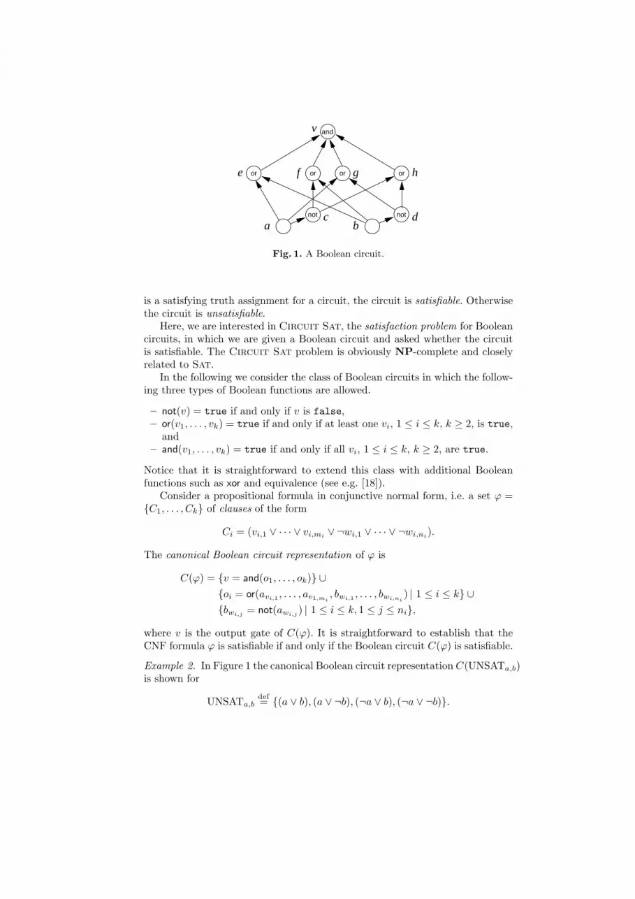
Formally, we present a Boolean circuit C with the set of gates V as a setof equations of the form v = f(v1, . . . , vk), where v, v1, . . . , vk ∈ V and f is aBoolean function. It is required that (i) each v ∈ V has at most one equation,(ii) the equations are non-recursive, and (iii) exactly one gate (i.e. the outputgate) does not appear on the right hand side of any equation. We define the sizeof a Boolean circuit to be the number of gates and edges in the circuit. For aBoolean circuit C, we denote the set of gates appearing in C by V (C).Example 1. Graphically, the Boolean circuit

{v = and(e, f, g, h), e = or(a, b), f = or(b, c), g = or(a, d),h = or(c, d), c = not(a), d = not(b)}

is shown in Figure 1. In this circuit, a and b are input gates, c, d, e, f, g and hintermediate gates, and v is the output gate.

A truth assignment for a Boolean circuit C is a function τ : V (C) → {true, false}.Assignment τ is consistent if τ(v) = f(τ(v1), . . . , τ(vk)) holds for each equationv = f(v1, . . . , vk) in C. A consistent truth assignment that assigns true to theoutput gate of a circuit is a satisfying truth assignment for the circuit. If there

or or or

and

or

not not

bac d

fe g h

v

Fig. 1. A Boolean circuit.

is a satisfying truth assignment for a circuit, the circuit is satisfiable. Otherwisethe circuit is unsatisfiable.

Here, we are interested in Circuit Sat, the satisfaction problem for Booleancircuits, in which we are given a Boolean circuit and asked whether the circuitis satisfiable. The Circuit Sat problem is obviously NP-complete and closelyrelated to Sat.

In the following we consider the class of Boolean circuits in which the follow-ing three types of Boolean functions are allowed.

– not(v) = true if and only if v is false,– or(v1, . . . , vk) = true if and only if at least one vi, 1 ≤ i ≤ k, k ≥ 2, is true,

and– and(v1, . . . , vk) = true if and only if all vi, 1 ≤ i ≤ k, k ≥ 2, are true.

Notice that it is straightforward to extend this class with additional Booleanfunctions such as xor and equivalence (see e.g. [18]).

Consider a propositional formula in conjunctive normal form, i.e. a set ϕ ={C1, . . . , Ck} of clauses of the form

Ci = (vi,1 ∨ · · · ∨ vi,mi ∨ ¬wi,1 ∨ · · · ∨ ¬wi,ni).

The canonical Boolean circuit representation of ϕ is

C(ϕ) = {v = and(o1, . . . , ok)} ∪{oi = or(avi,1 , . . . , av1,mi

, bwi,1 , . . . , bwi,ni) | 1 ≤ i ≤ k} ∪

{bwi,j = not(awi,j ) | 1 ≤ i ≤ k, 1 ≤ j ≤ ni},

where v is the output gate of C(ϕ). It is straightforward to establish that theCNF formula ϕ is satisfiable if and only if the Boolean circuit C(ϕ) is satisfiable.

Example 2. In Figure 1 the canonical Boolean circuit representation C(UNSATa,b)is shown for

UNSATa,bdef= {(a ∨ b), (a ∨ ¬b), (¬a ∨ b), (¬a ∨ ¬b)}.

3 A Tableau Method

We study a tableau method for Boolean circuit satisfiability checking we callBC. The method consists of the rules shown in Figure 2. It is a simplifiedversion of the tableau system introduced in [18].1 The method is a non-clausalgeneralisation of DPLL to Boolean circuits: the explicit cut rule (a) in BCcorresponds to the splitting rule in DPLL, and the rules (b)-(h) correspond tounit clause propagation, i.e., standard Boolean constraint propagation.

v ∈ VTv Fv

(a) The explicit cut rule

v = not(v1)Fv1

Tv

v = not(v1)Tv1

Fv

v = not(v1)Fv

Tv1

v = not(v1)Tv

Fv1

(b) “Up” rules for not (c) “Down” rules for not

v = or(v1, . . . , vk)Fv1, . . . ,Fvk

Fv

v = or(v1, . . . , vk)Tvi, i ∈ {1, . . . , k}

Tv

v = or(v1, . . . , vk)Fv

Fv1, . . . ,Fvk

(d) “Up” rules for or (e) “Down” rule for or

v = and(v1, . . . , vk)Tv1, . . . ,Tvk

Tv

v = and(v1, . . . , vk)Fvi, i ∈ {1, . . . , k}

Fv

v = and(v1, . . . , vk)Tv

Tv1, . . . ,Tvk

(f) “Up” rules for and (g) “Down” rule for and

v = or(v1, . . . , vk)Fv1, . . . ,Fvj−1,Fvj+1, . . .Fvk

Tv

Tvj

v = and(v1, . . . , vk)Tv1, . . . ,Tvj−1,Tvj+1, . . .Tvk

Fv

Fvj

(h) “Last undetermined child” rules for or and and

Fig. 2. Tableau method BC for Boolean circuits.

Given a Boolean circuit C, a BC-tableau for C is a binary tree such that theroot node of the tree consists of the equations in C and additionally the entryTv, where v is the output gate of C. The other nodes in the tree are entries of theform Tv or Fv, where v ∈ V (C), generated by extending the tableau using therules in Figure 2 in the following standard way [6]. Given a tableau rule and abranch in the tableau such that the prerequisites of the rule hold in the branch,the tableau can be extended by adding new nodes to the end of the branch as

1 The method introduced in [18] provides additionally, e.g., rules for xor and equiva-lence gates as well as circuit simplification rules.

specified by the rule. If the rule is (a), then entries Tv and Fv are added as theleft and right child in the end of the branch. For the other rules, the consequentsof the rule are added to the end of the branch (as a linear subtree in case ofmultiple consequents).

A branch in the tableau is contradictory if it contains both Fv and Tv entriesfor a gate v ∈ V (C). Otherwise, the branch is open. A branch is complete if it iscontradictory, or if there is a Fv or a Tv entry for each v ∈ V (C) in the branchand the branch is closed under the rules (b)–(h). A tableau is finished if all thebranches of the tableau are complete. A tableau is closed if all of its branches arecontradictory. A closed BC-tableau for a circuit is called a BC-refutation forthe circuit. For each v ∈ V (C), we say that the entry Tv (Fv) can be deduced ina branch if the entry Tv (Fv) can be generated by applying rules (b)–(h) only.

Example 3. For the circuit shown in Figure 1, a BC-refutation is shown in Figure3. For instance, in the refutation the entry Fc (15) is deduced from the entriesc = not(a) and Ta, while Ta (13) is generated by applying the cut rule.

1. v = and(e, f, g, h)2. e = or(a, b)3. f = or(b, c)4. g = or(a, d)5. h = or(c, d)6. c = not(a)7. d = not(b)8. Tv

9. Te (1, 8)10. Tf (1, 8)11. Tg (1, 8)12. Th (1, 8)

13. Ta (Cut)15. Fc (6, 13)16. Tb (3, 10, 15)17. Fd (7, 16)18. Fh (5, 15, 17)19. × (12, 18)

14. Fa (Cut)20. Tb (2, 9, 14)21. Td (4, 11, 14)22. Fd (7, 20)23. × (21, 22)

Fig. 3. A BC-refutation for C(UNSATa,b).

We study variations of BC in which the application of the explicit cut rule isrestricted to certain types of gates. The idea is to study the effects of restrictionswhich are based on the circuit structure. A natural starting point is a systemwhere cuts are restricted to input gates only. A dynamic generalisation of thisidea is to allow bottom-up cuts, i.e., to start from the input gates and permit

the use of the cut rule in a tableau branch for a gate only when an entry for oneof its children in the circuit has been deduced in the branch. A dual approachis to start from the entry of the output gate and allow top-down cuts. It is alsopossible to combine these approaches. The considered variations of BC are thusthe following.

– BCi: Application of explicit cut is restricted to input gates (input cuts).– BCbu: Application of explicit cut in a branch is restricted to input cuts and

gates v for which there is a Tv′ or a Fv′ entry in the branch for some childv′ of v in the circuit (bottom-up cuts).

– BCtd: Application of explicit cut in a branch is restricted to the output gateand gates v for which there is a Tv′ or a Fv′ entry in the branch for someparent v′ of v in the circuit (top-down cuts).

– BCi+td: Application of explicit cut is restricted to input and top-down cuts.– BCbu+td: Application of explicit cut is restricted to bottom-up and top-down

cuts.

By soundness we mean that the existence of a closed tableau for a givencircuit implies that the circuit is unsatisfiable, and by completeness that thereis a closed tableau for any unsatisfiable circuit.

The following soundness theorem follows straightforwardly from the observa-tion that the deduction rules (b)–(h) preserve satisfiability, i.e., if the premisesof a rule are consistent for a truth assignment, then so is the conclusion.

Theorem 1. BCi, BCtd, BCi+td, BCbu, BCbu+td, and BC are sound proofsystems for Boolean circuits.

The following completeness theorem is obvious by the cut rule. Input cutswith the deduction rules (b)–(h) are sufficient in order to obtain a completebranch. Moreover, input cuts can be simulated with top-down cuts in a straight-forward manner.

Theorem 2. BCi, BCtd, BCi+td, BCbu, BCbu+td, and BC are completeproof systems for Boolean circuits.

4 Propositional Proof Complexity and Simulation

Generally, a propositional proof is a certificate for the unsatisfiability of a propo-sitional expression (e.g., of a propositional formula or Boolean circuit). A propo-sitional proof system (see e.g. [2]) for a class of propositional expressions E isthen a polynomial-time computable predicate T such that for all expressionsα ∈ E it holds that α is unsatisfiable if and only if there is a proof P for α suchthat T (α, P ). If such a P exists, it is a T -proof for α.

For instance, resolution is a propositional proof system that produces proofsfor the unsatisfiability (i.e. refutations) of propositional formulas in conjunctivenormal form. Similarly, BC is a propositional proof system for the unsatisfiabilityof Boolean circuits.

Let T be a proof system. The proof complexity (or complexity in short) of apropositional expression α in T is the size of a minimal T -proof for α. The size ofa resolution refutation is defined in the standard way as the number of resolutionsteps in the refutation sequence. We define the size of a BC-refutation as thenumber of nodes in the closed tableau. For example, the size of the BC-refutationshown in Figure 3 is 14.

We use the notion of polynomial simulation to study the relative efficiency ofproof systems. For any two proof systems T and T ′, we say that T polynomiallysimulates T ′, denoted by T º T ′, if there is a polynomial q such that, for any α,if there is a T ′-proof for α of size n, then there is a T -proof for α of size at mostq(n). Hence, T º T ′ indicates that the proof system T is at least as strong asT ′ (up to a polynomial loss of efficiency). The relation º is transitive. If T º T ′

holds but T ′ º T does not, we write T Â T ′. If neither T º T ′ nor T ′ º T holds,we write T # T ′.

We denote by ºχ the restricted form of polynomial simulation, in whichT ºχ T ′ holds if there is a polynomial q such that, for any α ∈ χ, if there isa T ′-proof for α of size n, then there is a T -proof for α of size at most q(n). Ifboth T ºχ T ′ and T ′ ºχ T hold, we write T ≡χ T ′.

An obvious ordering of BC and its restricted variations based on the polyno-mial simulation relation, resulting from the restricted nature of the variations,is shown in Figure 4.

BCbu

º ºBC º BCbu+td BCi

º ºBCi+td

ºBCtd

Fig. 4. An obvious ordering of BC and its variations based on the polynomial simula-tion relation.

It turns out that all the considered variations of the BC method are equiv-alent under the polynomial simulation relation when the set of propositionalexpressions considered is restricted to the set of canonical Boolean circuit rep-resentations of sets of clauses. For the following, let Φ be the family of all setsof clauses, and C(Φ) = {C(ϕ) | ϕ ∈ Φ}.Theorem 3. BC ≡C(Φ) BCi.

To see this, notice that for any set of clauses ϕ, using the “down” rule for andwe can deduce Tg for all or gates g in C(ϕ). Thus we can assume that there is aminimal-size refutation for C(ϕ) in which the and rule is applied to deduce theentries concerning the or gates that are needed to achieve the closed tableau.

Then it is straightforward to see that we can limit the application of the cut ruleto input gates. This shows BCi ºC(Φ) BC, while BC ºC(Φ) BCi holds trivially.

By further noticing that for any circuit in the family C(Φ) input cuts canbe polynomially simulated with top-down cuts in a straightforward manner, wehave the following corollary.

Corollary 1. BC ≡C(Φ) T for all T ∈ {BCi,BCtd,BCi+td,BCbu}.The following theorem states that, for the canonical Boolean circuit repre-

sentation of a set of clauses, BC-proofs can be simulated by tree-like resolution.This is fairly straightforward to establish from a well-known construction forreading a tree-like resolution refutation from a DPLL refutation, see e.g. [1].

Theorem 4. There is a polynomial p such that for any set of clauses ϕ, ifthere is a BC-refutation for C(ϕ) of size n, then there is a tree-like resolutionrefutation for ϕ of size p(n).

Again, by the restricted nature of the variants of the BC method, we have thefollowing corollary.

Corollary 2. For each T ∈ {BCi,BCtd,BCi+td,BCbu,BCbu+td} it holds thatthere is a polynomial p such that for any set of clauses ϕ, if there is a T -refutationfor C(ϕ) of size n, then there is a tree-like resolution refutation for ϕ of size p(n).

We note that tree-like resolution (and thus DPLL) and BC are equally efficientproof systems in the sense that (i) given a set of clauses ϕ, BC on C(ϕ) canpolynomially simulate tree-like resolution on ϕ and, moreover, (ii) given a circuitC and the set of clauses ϕC obtained from C using Tseitin’s translation, DPLLand thus tree-like resolution on ϕC can polynomially simulate BC on C. Thelatter fact is discussed in more detail in Section 6 in which it is shown that therules of BC match those of DPLL.

5 Relative Efficiency of Restricted Cuts

The main results of this paper are summarised in Figure 5 showing that thereis no two-way polynomial simulation between the variations of the BC method.The results shed new light on the strength of proof systems of this kind, where thestrength of the system is measured as the size of the minimal proofs produciblefor a given proposition. The results show that it is possible to increase thestrength of a system significantly by extending the use of the cut rule in acontrolled local manner w.r.t. the circuit structure. For example, moving frominput cuts to bottom-up cuts can make a substantial difference in the sense thatinput cuts cannot polynomially simulate bottom-up cuts. If top-down cuts areadditionally allowed, a similar substantial increase in the strength of the systemis obtained. However, general cuts are still substantially stronger than any of therestricted variations considered. It should be noticed that the results obviouslyhold for circuits with additional Boolean functions if the set of rules involvingand, or, and not gates remains unchanged. Furthermore, the results imply that

the restrictions on the splitting rule in DPLL have the same effect on the proofcomplexity of CNF formulas obtained from Boolean circuits by using Tseitin’stranslation as will be discussed in Section 6.

The rest of this section is devoted to proofs of these results. The proofs relyon certain circuit families which are constructed from building blocks such as aBoolean circuit representation of the pigeon-hole principle. First we define thebuilding blocks we call gadgets and then give the proofs of the main theorems 6–14. Combining these theorems, the resulting ordering of BC and its restrictedvariations based on the polynomial simulation relation, shown in Figure 5, isobtained by the transitivity of º.

5.1 Gadget Constructions

We begin by defining the PHPn+1n , TDn, XORn, and UNSAT gadgets. They

are used in constructing families of circuits which are used in proving the maintheorems of this paper. Some lemmas involving properties of the gadgets aregiven.

Pigeon-Hole Principle and the PHPn+1n Gadget An example of a propo-

sitional formula with high proof complexity in many proof systems is the pigeon-hole principle PHPm

n , see e.g. [16]. The pigeon-hole principle states that thereis no injective mapping from a finite m-element set into a finite n-element set ifm > n (that is, m pigeons cannot sit in less than m holes so that every pigeonhas its own hole). In the following we consider the case m = n + 1. As a set ofclauses, we have

PHPn+1n

def=⋃

1≤i≤n+1

{Pi} ∪⋃

1≤i<i′≤n+1,1≤j≤n

{Hji,i′},

where the clauses Pi and Hji,i′ are defined as Pi

def=∨n

j=1 xi,j and Hji,i′

def= (¬xi,j∨¬xi′,j), and each xi,j is a Boolean variable with the interpretation “xi,j = trueif and only if the ith pigeon sits in the jth hole”. The Pi clauses state that each

BCbu

 ÂBC  BCbu+td # BCi

 ÂBCi+td #

ÂBCtd

Fig. 5. Summary of the ordering of BC and its restricted variations based on thepolynomial simulation relation. The case BCbu # BCtd is omitted from the picturefor clarity.

pigeon has to sit in some hole, while clauses Hji,i′ state that no two pigeons can

sit in the same hole. The union of all the clauses Pi and Hji,i′ is obviously (by

the pigeon-hole principle) unsatisfiable.The canonical Boolean circuit representation of PHPn+1

n is shown in part inFigure 6(a). We call C(PHPn+1

n ) the PHPn+1n gadget. Notice that as PHPn+1

n

is unsatisfiable, so is C(PHPn+1n ). Formally the PHPn+1

n gadget is the set of

and

or or

xi,jxi’,j

i’,jl

i,i’j

i

notnot

ph

i,jl

v

(a)

or

and and

orxn

x1z 1 y1

xn

vn wn

vn+1

and and

or

1

yn

n

v

v1 w1

z n

wn+1

T

T

(b)

Fig. 6. (a) A part of the PHPn+1n gadget in detail, (b) the structure of the TD gadget.

equations

C(PHPn+1n ) = {v = and(p1, . . . , pn+1, h

11,2, . . . , h

nn+1,n)} ∪

{pi = or(xi,1, . . . , xi,n) | 1 ≤ i ≤ n + 1} ∪{hj

i,i′ = or(li,j , li′,j) | 1 ≤ i < i′ ≤ n + 1, 1 ≤ j ≤ n} ∪{li,j = not(xi,j) | 1 ≤ i ≤ n + 1, 1 ≤ j ≤ n},

where h11,2, . . . , h

nn+1,n stands for all hj

i,i′ , where 1 ≤ i < i′ ≤ n+1 and 1 ≤ j ≤ n.By the results in [15] we have the following theorem.

Theorem 5. The size of the minimal resolution refutations for PHPn+1n is ex-

ponential w.r.t. n.

Combining Theorem 4, Corollary 2, and Theorem 5, we have the following corol-lary.

Corollary 3. For each T ∈ {BCi,BCtd,BCi+td,BCbu,BCbu+td,BC}, thesize of the minimal T -refutations for C(PHPn+1

n ) is exponential w.r.t. n.

We use the pigeon-hole principle formulas because they are well-known and thefamily {PHPn+1

n } has some nice features: (i) the size of each PHPn+1n CNF

instance is polynomial w.r.t. n, and (ii) the size of the minimal resolution refu-tation for PHPn+1

n is exponential w.r.t. n. Notice that other hard CNF formulafamilies with similar properties could have been used instead.

The TD Gadget The structure of the TDn gadget is shown in Figure 6(b).Formally the TDn gadget is the set of equations

TDn = {v = or(v1, w1)} ∪{vi = and(xi, zi) | 1 ≤ i ≤ n} ∪{wi = and(yi, zi) | 1 ≤ i ≤ n} ∪{zi = or(vi+1, wi+1) | 1 ≤ i ≤ n}.

The following lemma on the TDn gadget will be useful in the proofs of our mainresults. This lemma derives from the fact that in order to have an entry for gatezn in every branch of a BCtd tableau, one has to apply the cut rule on vi or wi

for each 1 ≤ i ≤ n, which leads to having an exponential number of entries inthe tableau w.r.t. n.

Lemma 1. Every BCtd-tableau for TDn in which each branch has an entry forthe gate zn is of exponential size w.r.t. n.

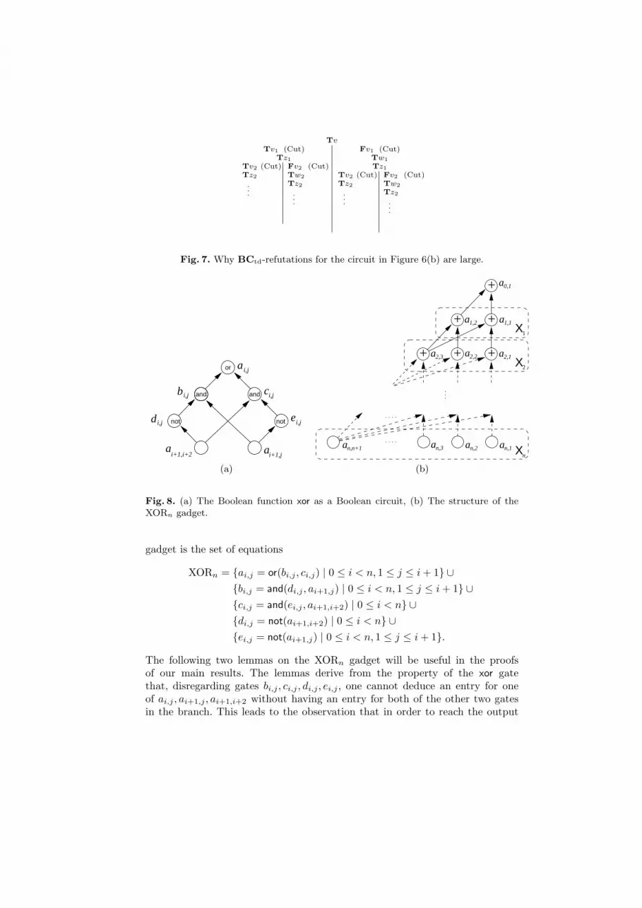
Proof. The entry Tv implies Tv1 or Tw1, but we cannot deduce one or theother. Thus we must apply the cut rule on either v1 or w1 in BCtd. Assume thatwe cut on v1 (cutting on w1 is symmetric). Now consider the branch in which wehave Fv1. Due to v = or(v1, w1) we must have Tw1. Then from w1 = and(y1, z1)we deduce Ty1 and Tz1 in the branch. In the branch where we have Tv1 usingthe “down” rule for and we deduce Tx1 and Tz1. Nothing else can be deduced.Inductively on i, in order to have an entry for the gate zi in every branch of thetableau, the tableau must contain at least 2i branches, all of which remain open.This is because we must for each i apply the cut rule on either vi or wi. This isdemonstrated in Figure 7. Thus every tableau in which there is an entry for thegate zn in every branch of the tableau is of size at least in the order of 2n, thatis, 2|V (TDn)|/5.

The XOR Gadget The Boolean xor function xor(x, y) = (x ∧ ¬y) ∨ (¬x ∧ y)evaluates to true if and only if exactly one of x, y is true. Based on the xorfunction we can construct a Boolean circuit, as shown in Figure 8(a), for which itholds that the output gate ai,j evaluates to true if and only if xor(ai+1,i+2, ai+1,j)evaluates to true. When we use this circuit construct as a part of a circuit, werepresent it graphically as an “xor gate” ⊕.

Using the “xor gate” we construct a family of XORn gadgets as shown inFigure 8(b), having n layers Xi, 1 ≤ i ≤ n, of xor gates. Formally, the XORn

TvTv1 (Cut)

Tz1Tv2 (Cut)Tz2

.

.

.

Fv2 (Cut)Tw2Tz2

.

.

.

Fv1 (Cut)Tw1Tz1

Tv2 (Cut)Tz2

.

.

.

Fv2 (Cut)Tw2Tz2

.

.

.

Fig. 7. Why BCtd-refutations for the circuit in Figure 6(b) are large.

or

andand

a

c

enotnot

b

d i,j

i,j

i,j

i,j

i,j

i+1,i+2a ai+1,j

(a)

+

a2,1

a1,1X1

X2

+

an,n+1 an,3 an,2 an,1

++

a1,2

a2,2

+

Xn

a0,1

+a2,3

(b)

Fig. 8. (a) The Boolean function xor as a Boolean circuit, (b) The structure of theXORn gadget.

gadget is the set of equations

XORn = {ai,j = or(bi,j , ci,j) | 0 ≤ i < n, 1 ≤ j ≤ i + 1} ∪{bi,j = and(di,j , ai+1,j) | 0 ≤ i < n, 1 ≤ j ≤ i + 1} ∪{ci,j = and(ei,j , ai+1,i+2) | 0 ≤ i < n} ∪{di,j = not(ai+1,i+2) | 0 ≤ i < n} ∪{ei,j = not(ai+1,j) | 0 ≤ i < n, 1 ≤ j ≤ i + 1}.

The following two lemmas on the XORn gadget will be useful in the proofsof our main results. The lemmas derive from the property of the xor gatethat, disregarding gates bi,j , ci,j , di,j , ei,j , one cannot deduce an entry for oneof ai,j , ai+1,j , ai+1,i+2 without having an entry for both of the other two gatesin the branch. This leads to the observation that in order to reach the output

gate with bottom-up cuts or an input gate with top-down cuts one must applythe cut rule a number of times linear in n, and thus to having an exponentialnumber of entries in the tableau w.r.t. n.

Lemma 2. Every BCbu-tableau for XORn in which each branch has an entryfor the gate a1,1 or a1,2 is of exponential size w.r.t. n.

Proof. We show by induction on n that every BCbu-tableau for XORn in whicheach branch has an entry for the gate a1,1 or a1,2 is of size at least 2n.

For n = 1, we must use the cut rule first on a1,2 or a1,1. Thus the branch has1 application of the cut rule and the whole tableau is at least of size 21.

Now assume that the lemma holds for n. Suppose that for XORn+1 there isa BCbu-tableau of size less than 2n+1 in which there is in each branch an entryfor a1,1 or a1,2. In such a tableau, we must use the cut rule first on one of thegates an+1,j , 1 ≤ j ≤ n + 2. Due to the xor-nature of the a gates and the use ofbottom-up cuts, no gate of form ak,l, k ≤ n, can have a deduced entry before wehave an entry for the gate an+1,n+2 (produced either (i) by a cut on an+1,n+2,or (ii) by a cut on an undetermined gate bn,j or cn,j such that a cut was alreadymade on an+1,j , forcing an entry for an+1,n+2, too). Therefore, we can assumethat the first cut was actually made on an+1,n+2. Because of the assumptionthat the size of the tableau is less than 2n+1, one of the sub-tableaux below thiscut has size less than 2n. In such a sub-tableau, if the gate an+1,n+2 has an entryFan+1,n+2, the gate an,m has an entry Fan,m (Tan,m) if and only if the gatean+1,m has an entry Fan+1,m (Tan+1,m). Similarly, if the gate an+1,n+2 has anentry Tan+1,n+2, the gate an,m has an entry Fan,m (Tan,m) if and only if thegate an+1,m has an entry Tan+1,m (Fan+1,m). Therefore, if we have made a cuton a gate an+1,m in the sub-tableau, we could have equivalently made a cut onan,m. By replacing each such cut on an+1,m with a cut on an,m and removingother entries on gates not appearing in XORn, we transform the sub-tableaufor XORn+1 to a BCbu-tableau for XORn having size less than 2n. But thiscontradicts the induction hypothesis and thus both sub-tableaux must have sizeat least 2n and the whole BCbu-tableau for XORn+1 is of size at least in theorder of 2n+1.

Lemma 3. Every BCtd-tableau for XORn in which each branch has an entryfor some gate an,i, 1 ≤ i ≤ n + 1, is of exponential size w.r.t. n.

Proof. As shown in Figures 9 and 10, in order to deduce an entry for ai+1,j orai+1,i+2 from an entry for ai,j , one has to apply the cut on one of the gates inthe xor gate. This causes branching, while no branches can be closed.

By branching on b0,1 (or symmetrically on c0,1), we can thus deduce entriesfor both a1,1 and a1,2 in both branches. Thus in each branch we may continueas in either of Figures 9 or 10. Notice that after branching we have an entry forai+1,i+2 in every branch. In addition to entries for all ai,j , where 1 ≤ j ≤ i + 1,this is enough to deduce entries for all ai+1,j . Still, for every i, we must apply thecut on some gate on level i to deduce entries for the gates ai+1,j , 1 ≤ j ≤ i + 2,doubling the number of open branches for each i. Thus every tableau in which

1. Fai,j

2. Fbi,j

3. Fci,j

4. Tai+1,j (Cut)6. Fdi,j (2, 4)7. Tai+1,i+2 (6)8. Fei,j (4)

5. Fai+1,j (Cut)9. Tei,j (5)10. Fai+1,i+2 (3, 9)11. Tdi,j (10)

Fig. 9. A top-down sub-tableau for the xor circuit with an Fai,j entry.

1. Tai,j

2. Tbi,j (Cut)4. Tdi,j (2)5. Tai+1,j (2)6. Fai+1,i+2 (4)7. Fci,j (6)8. Fei,j (5)

3. Fbi,j (Cut)9. Tci,j (1, 3)10. Tai+1,i+2 (9)11. Tei,j (9)12. Fai+1,j (11)13. Fdi,j (10)

Fig. 10. A top-down sub-tableau for the xor circuit with a Tai,j entry.

there is in every branch an entry for some gate an,i, 1 ≤ i ≤ n + 1, is of size at

least in the order of 2n, that is, 2√|V (XORn)|.

5.2 BCbu vs BCi

We now show that BCi cannot polynomially simulate BCbu. The proof utilisesthe UNSAT (i.e., the circuit shown in Figure 1) and PHPn+1

n gadgets.

Lemma 4. There is an infinite family {Cn} of circuits such that (i) the size ofCn is O(n3), and (ii) there is a BCbu-refutation for Cn of constant size whileany minimal BCi-refutation for Cn is of size exponential in n.

Proof. Consider the family of circuits of the type shown in Figure 11(a). Anycircuit in the family is obviously unsatisfiable. For an arbitrary n, for BCbu wecan construct a constant size refutation as follows. First, deduce Te, Tf , Tg,Th from Tv. Then apply (say, in the PHPn+1

n gadget on the left) the cut rulefirst on one of the input gates xi,j , and deduce an entry for li,j . After this, applythe cut rule on hj

i,i′ in both of the induced branches. Now we have induced fourbranches in total, having in each branch a constant number of entries, and canapply the cut rule on a in each branch. After having an entry on a, each branchcan be closed in a constant number of steps similarly to the refutation shown inFigure 3. Thus the generated closed tableau is of constant size.

Notice that to generate a refutation we need to reach the UNSAT gadget,i.e., it is impossible to generate a contradiction in all the branches of a tableauwithout having an entry for some of the gates in the UNSAT gadget in thetableau.

Now consider BCi. From Tv we can deduce Te, Tf , Tg, and Th, but nothingelse. As PHPn+1

n is unsatisfiable, it is impossible to deduce Ta or Tb with “up”rules. Thus we can only have Fa and Fb entries in any branch. In addition, aclosed tableau can only be achieved after deducing an entry for gate a or gateb. Thus we must have either Fa or Fb in every branch. But if we have Fa or Fbin every branch, then we effectively have a BCi-refutation for C(PHPn+1

n ). ByCorollary 3, the size of such a refutation must be exponential in n.

Theorem 6. BCbu  BCi.

Proof. Obviously, BCbu º BCi. By Lemma 4, there is a family {Cn} of circuitsfor which BCbu has constant size refutations while the minimal BCi-refutationsare of exponential size w.r.t. the circuit index n. As the size of the circuit Cn isO(n3), the minimal BCi-refutations are of size super-polynomial in the size ofthe circuit. Based on these facts, BCi º BCbu cannot hold.

5.3 BCi+td vs BCi

We now proceed to show that BCi cannot polynomially simulate BCi+td. Thisfollows directly from the following lemma. In the proof, we re-use the ideasemployed in the proof of Lemma 4.

Lemma 5. There is an infinite family {Cn} of circuits such that (i) the size ofCn is O(n3), and (ii) there is a BCi+td-refutation for Cn of constant size whileany minimal BCi-refutation for Cn is of exponential size w.r.t. n.

Proof. Consider again the family of circuits of the type shown in Figure 11(a).We have that any circuit in the family is unsatisfiable. For BCi+td we canconstruct a constant size refutation by first deducing Te, then applying the cutrule on gate a, and then closing each branch similarly to the refutation shownin Figure 3. For BCi, all BCi-refutations will be of exponential size w.r.t. n asargued in the proof of Lemma 4.

Theorem 7. BCi+td  BCi.

5.4 BCi+td vs BCtd

Next we show that BCtd cannot polynomially simulate BCi+td by establish-ing the following lemma. The proof is based on a circuit constructed from twoUNSAT gadgets and a TDn gadget.

Lemma 6. There is an infinite family {Cn} of circuits such that (i) the size ofCn is O(n), and (ii) there is a BCi+td-refutation for Cn of linear size while anyminimal BCtd-refutation for Cn is of exponential size w.r.t. n.

n+1PHPnn+1PHPn

v

and and

UNSATa,bba

and

(a)

a ,b2 2a ,b

v

and and w

UNSAT1 1

UNSAT

TDn

n+1vn+1

or

(b)

Fig. 11. (a) Circuit for Theorems 6 and 7. (b) Circuit for Theorem 8.

Proof. Consider the family of circuits of the type shown in Figure 11(b). Anycircuit in this family is obviously unsatisfiable. For BCi+td we can constructa refutation of linear size w.r.t. n as follows. First apply consecutively the cutrule on gates a1, b1, a2, b2 in each branch. This induces 16 branches, a constantnumber. We then have an entry for each of a1, b1, a2, b2 in every branch. Nowwe can deduce an entry for vn+1 and wn+1 in each branch. As C(UNSATa,b) isunsatisfiable, we can only deduce Fvn+1 and Fwn+1. This can clearly be done ina constant number of steps. From the entries Fvn+1, Fwn+1 we can then deduceFzn, and then Fvn, Fwn. Proceeding recursively, we can thus deduce Fv in everybranch with a linear number of steps w.r.t. n.

Notice that to generate a refutation we need to reach the UNSAT gadgets,as in the proof of Lemma 4. But by Lemma 1, before reaching the gate zn

top-down, we already must have generated a tableau with exponentially manyentries w.r.t. n. Every BCtd-refutation is thus of exponential size w.r.t. n forthis family of circuits.

Theorem 8. BCi+td  BCtd.

5.5 BCbu+td vs BCi+td

In this subsection we show that BCi+td cannot polynomially simulate BCbu+td.Using the ideas in the proof of Lemma 4, we construct a circuit from threecircuits similar to the one employed in the proofs of Lemmas 4 and 5, an XORn

gadget, and an expander sub-circuit that connects the former four. The expandercircuit is an example of a simple nontrivial circuit in which deduction can bepropagated through the circuit in a straightforward fashion. It is applied here sothat trivial simplification of the circuit is not possible. Lemma 3 is also applied.

Lemma 7. There is an infinite family {Cn} of circuits such that (i) the size ofCn is O(n3), and (ii) there is a BCbu+td-refutation for Cn of size O(n2) whileany minimal BCi+td-refutation for Cn is of exponential size w.r.t. n.

Proof. Consider the family of circuits of the type shown in Figure 12. Any cir-cuit in the family is unsatisfiable. For BCbu+td we can construct a refutation

an,n+1an,1

+XOR

n

and

PHP

and

PHP

and

PHP

and

PHP

and

PHP

and

PHP

v2v1 v3

a1 a2 a3b1 b2 b3

or or or or

or or andor

or andor

and

and

and

and

and and and

v

UNSAT UNSAT UNSAT

Fig. 12. Circuit for Theorem 9.

of polynomial size w.r.t. n as follows. First apply the bottom-up strategy intro-duced in the proof of Lemma 4 to work through the PHPn+1

n gadgets and togenerate entries for the and gates a1, a2, a3, b1, b2, b3 in every branch. As in theproof of Lemma 4, this can be done having a constant number of entries in thetableau. Then it is straightforward to deduce entries for v1, v2, v3 in each branch.Furthermore, as C(UNSATa,b) is unsatisfiable, we must then have Fv1,Fv2,Fv3

in every branch. Now in an arbitrary branch, it is straightforward to deduce theentries Fan,j for all 1 ≤ j ≤ n + 1, generating only a number of entries in theorder of n2. Continuing on, generating only a number of entries in the order ofn2, deducing recursively Fai−1,j from Fai,j and Fai,i+1 we can at last deduceFv. As we have in total a constant number of branches and O(n2) entries ineach branch, we clearly have a BCbu+td-refutation of size O(n2).

Again, to generate a refutation we need to reach the UNSAT gadgets. Withinput cuts, this results in a refutation of exponential size w.r.t. n, as argued inthe proof of Lemma 4. By Lemma 3, any top-down approach will also result ina refutation of exponential size w.r.t. n.

Theorem 9. BCbu+td  BCi+td.

5.6 BCbu+td vs BCbu

Next we show that BCbu cannot polynomially simulate BCbu+td. In additionto ideas employed in the proof of Lemma 5, we use a circuit constructed from apair of XORn gadgets and an UNSAT gadget, and apply Lemma 2.

Lemma 8. There is an infinite family {Cn} of circuits such that (i) the size ofCn is O(n2), and (ii) there is a BCbu+td-refutation for Cn of constant size whileany minimal BCbu-refutation for Cn is of exponential size w.r.t. n.

Proof. Consider the family of circuits of the type shown in Figure 13(a). AsC(UNSATa,b) is unsatisfiable, any circuit in this family is also unsatisfiable.

As already described in the proof of Lemma 5, for BCbu+td we can constructa constant size refutation top-down by first deducing Te, then applying the cutrule on gate a, and closing each branch similarly to the refutation shown inFigure 3.

It is impossible to generate a refutation without reaching the UNSAT gadgets,as in the previous proofs in which we had an UNSAT gadget as a part of thecircuit. By Lemma 2, in order to reach the UNSAT gadget, we must generate atableau with exponential number of branches w.r.t. n. Thus any BCbu-refutationfor any circuit in this family must be of exponential size w.r.t. n.

Theorem 10. BCbu+td  BCbu.

5.7 BC vs BCbu+td

Now we proceed by showing that BCbu+td cannot polynomially simulate BC.The proof uses n + 1 UNSAT gadgets and 2n + 3 XORn gadgets, and appliesLemmas 2 and 3.

Lemma 9. There is an infinite family {Cn} of circuits such that (i) the size ofCn is O(n3), and (ii) there is a BC-refutation for Cn of size O(n2) while anyminimal BCbu+td-refutation for Cn is of exponential size w.r.t. n.

andv

UNSATa,b

+ + ba

n nXOR XOR

(a)

and

+

bn+1 a1 b1++n+1aUNSAT

1a 1b

XOR n XOR n

and

XORn

v

an,1an,n+1

+UNSAT ba n+1n+1

XORn

+XORn

(b)

Fig. 13. (a) Circuit for Theorem 10. (b) Circuit for Theorem 11.

•Tan,1

ttiiiiiiiiiiiiiiiiiiii

Fan,1

²²UNSATa1,b1 •

Tan,2

ttiiiiiiiiiiiiiiiiiiii

Fan,2

²²UNSATa2,b2 •

²²•

Tan,n+1

ttiiiiiiiiiiiiiiiiiiii

Fan,n+1

²²UNSATan+1,bn+1 {Fan−1,j | 1 ≤ j ≤ n}

²²{Fan−2,j | 1 ≤ j ≤ n− 1}

²²{Fa1,1,Fa1,2}

²²Fv

Fig. 14. How to generate a polynomial size BC-refutation for the circuit shown inFigure 13(b).

Proof. Consider the family of circuits of the type shown in Figure 13(b). For BCwe can construct a refutation of polynomial size w.r.t. n as follows. First applythe cut rule on an,1. In the branch in which we have Tan,1, apply the cut ruleon a1. Similarly to the refutation in Figure 3, we can close both the branch inwhich we have Ta1 and the one in which we have Fa1. In the branch in whichwe have Fan,1, recursively on i, cut first on an,i and then in the branch in whichwe have Tan,i, cut on ai and again close both of the induced branches. This ideais shown in Figure 14. As the refutation in Figure 3 is of constant size, we endup with a tableau of linear size w.r.t. n in which there is a single open branchwith the entries Fan,i for all 1 ≤ i ≤ n + 1. After this, generating only numberof entries in the order of n2, deducing recursively Fai−1,j from Fai,j and Fai,i+1

we can at last deduce Fv, thus generating a BC-refutation of size O(n2).Again, to generate a refutation we need to reach the UNSAT gadgets. By

Lemma 2, any bottom-up approach will result in a refutation of exponential sizew.r.t. n. By Lemma 3, this applies also for any top-down approach. Thus anyBCbu+td-refutation will be of exponential size w.r.t. n for any circuit in thisfamily.

Theorem 11. BC Â BCbu+td.

5.8 BCi vs BCtd

We now turn to show that BCi and BCtd are incomparable under the polynomialsimulation relation. The proof draws heavily on the proofs of Lemmas 4 and 6.

Theorem 12. BCi # BCtd.

Proof. Consider again the family of circuits shown in Figure 11(a). In the proofof Lemma 4 it is shown that all BCi-refutations for any circuit in this family areof exponential size w.r.t. n. For an idea of how to generate a BCtd-refutation ofconstant size we again refer the reader to the refutation shown in Figure 3.

On the other hand, consider the family {Cn} of circuits shown in Figure 11(b).By the proof of Lemma 6 any minimal BCtd-refutation for Cn is of exponentialsize w.r.t. n, while in the same proof it is described how to construct a linearsize refutation for Cn by applying the cut rule only on input gates.

5.9 BCbu vs BCtd

Using ideas from the proof of Lemma 8 and Theorem 12, we show that BCbu

and BCtd are incomparable under the polynomial simulation relation.

Theorem 13. BCbu # BCtd.

Proof. By Theorem 12 BCtd cannot polynomially simulate BCi. As BCbu ºBCi, BCtd cannot polynomially simulate BCbu either.

Consider the family {Cn} of circuits shown in Figure 13(a). It holds thatthere is a BCtd-refutation of constant size for each Cn, while any minimal BCbu-refutation is of exponential size w.r.t. n by the proof of Lemma 8.

5.10 BCbu vs BCi+td

As the last one of the main theorems of this work, we argue that BCbu andBCi+td are incomparable under the polynomial simulation relation.

Theorem 14. BCbu # BCi+td.

Proof. By Theorem 13, BCbu cannot polynomially simulate BCtd. As BCi+td ºBCtd, BCbu cannot polynomially simulate BCi+td either.

On the other hand, consider the family {Cn} of circuits shown in Figure 15.Notice that a circuit Cn consists of a TDn gadget from the input gates ofwhich hang two sub-circuits equivalent to the circuit in Figure 11(a). CombiningLemma 1 and the reasoning presented in the proof of Lemma 4, we have thatevery BCi+td-refutation for an arbitrary circuit in this family is of exponentialsize w.r.t. n, as it is impossible to reach the UNSAT gadgets using top-down andinput cuts without generating an exponential number of entries in the tableauw.r.t. n. For BCbu, we can generate a refutation of linear size w.r.t. n as follows.It is discussed in the proof of Lemma 4 how one can apply the cut on gate a inthe circuit in Figure 11(a). What we can do here is to cut through the PHPn+1

n

and

+

++ +a21a

and

v

wn+1

+n PHPn+1

n nn+1

PHPn+1PHPPHP n+1

n

TDn

n+1v

b1 b2

UNSATUNSAT

Fig. 15. Circuit for Theorem 14.

circuits similarly as in the proof of Lemma 4. Then we can apply the cut rule oneach gate a1, b1, a2, b2 in each branch. After this, it is straightforward to deducean entry for gates vn+1 and wn+1 in every branch. Due to the unsatisfiabilityof C(UNSATa,b), with this bottom-up approach it is only possible to deduceFvn+1,Fwn+1. At this point we note that as the UNSAT gadget with PHPn+1

n

gadgets hanging from the input gates has a constant number of gates, we have sofar obviously generated a tableau with constant number of entries only. HavingFvn+1,Fwn+1 in each branch, it is possible to deduce Fv by generating only alinear number of entries w.r.t. n, as explained in the proof of Lemma 6. Thuswe can generate a BCbu-refutation of linear size w.r.t. n for any member of thefamily of circuits considered.

6 Relevance to DPLL

Each Boolean circuit C can be translated into a propositional formula in CNF oflinear size w.r.t. the size of C so that the formula is satisfiable if and only if C is.Tseitin’s translation [30] is a standard approach, introducing a new variable vg

for each gate g in C and capturing the functional dependencies in C by clauses.The translation is summarised in Table 1. Clearly, it is linear in the number ofgates and edges in C. The output CNF formula is the union of the sets of clausesproduced by the translation. We now argue that the main results of this workapply to DPLL (without learning or non-chronological backtracking) in the casethat the input is in CNF translated from a circuit using Tseitin’s translation.

We assume that the reader is familiar with the basic DPLL. A DPLL-refutation can be abstractly seen as a tableau in which the entries are setsof clauses obtained by unit propagation and splitting. A branch in a tableau iscontradictory if there are both of the unit clauses (a) and (¬a) in the branchfor some variable a. The rest of the terminology concerning DPLL-tableaux issynonymous in an obvious way with that of BC-tableaux.

Table 1. Tseitin’s translation of a Boolean circuit to a set of clauses.

Boolean circuit clause set

g is the output gate {(vg)}g = not(g1) {(vg ∨ vg1), (¬vg ∨ ¬vg1)}

g = or(g1, . . . gk) {(vg1 ∨ · · · ∨ vgk ∨ ¬vg)} ∪⋃k

i=1{(vg ∨ ¬vgi)}

g = and(g1, . . . gk) {(¬vg1 ∨ · · · ∨ ¬vgk ∨ vg)} ∪⋃k

i=1{(¬vg ∨ vgi)}

For the following, let ϕ be a set of clauses that is obtained from a Booleancircuit using Tseitin’s translation. It holds that DPLL for ϕ can polynomiallysimulate BC for the original circuit, and vice versa. In fact, any DPLL-refutationcan be interpreted as a BC-refutation, and vice versa. Especially, we argue thatunit clauses (vg) ((¬vg)) in a DPLL-refutation correspond exactly to entries Tg(Fg) of the corresponding BC-refutation.

Obviously, the splitting rule in DPLL is equivalent to the cut rule in BC;adding the unit clause (vg) ((¬vg)), is equivalent to extending a branch with Tg(Fg) by applying the cut rule, and vice versa. It is also straightforward to seethat the unit propagation rule in DPLL and the deterministic tableau rules inFigure 2(b)–(h) in BC have equivalent deduction power. To demonstrate this,we consider the two following example cases.

Consider the last undetermined child rule for and gates. Assume a branchin which (i) a gate g = and(g1, . . . , gk) is constrained to false by having theentry Fg and (ii) all g1, . . . , gk−1 are constrained to true by having the entriesTg1, . . . ,Tgk−1. One can now deduce Fgk by applying the rule. This deductionstep can be simulated in the corresponding DPLL-tableau branch because thebranch has unit clauses (¬vg), (vg1),. . . , and (vgk−1). Thus the clause (¬vg1∨· · ·∨¬vgk

∨ vg) resulting from Tseitin’s translation of and gates can be transformedinto the unit clause (¬vgk

) by applying unit propagation.On the other hand, assume that it is possible to generate the unit clause (¬vg)

in a branch of the DPLL-tableau by unit propagating on an original clause ofform (vg1 ∨ · · · ∨ vgk

∨ ¬vg). This means that the branch must contain the unitclauses (¬vg1),. . . ,(¬vgk

). Thus the corresponding BC-tableau branch has theentries Fg1,. . . ,Fgk and the entry Fg can be deduced by applying an “up” ruleon the gate g = or(g1, . . . gk) that was translated to have the clause (vg1 ∨ · · · ∨vgk

∨ ¬vg) in the CNF formula.

7 Conclusion

This work addresses the question of how restrictions on the use of the cut rule af-fect proof complexity in Boolean circuit satisfiability checking based on tableaux.The tableau method in question consists of a complete and sound subset of therules in the method introduced in [18]. The results show that the methods ob-tained by the cut restrictions considered (any combination of input, top-down,and bottom-up cuts) cannot polynomially simulate the unrestricted method.Moreover, for each pair of restricted methods, there exist a family of circuits

{Cn} for which the sizes of the minimal proofs differ exponentially w.r.t. n be-tween the methods.

The introduced tableau method is a non-clausal generalisation of the Davis-Putnam-Logemann-Loveland method for CNF formulas. The results show thatDPLL with locality based cut restrictions, such as splitting on the input gatesonly, cannot polynomially simulate the DPLL method with an unrestricted split-ting rule. This, in turn, contradicts a common belief based on empirical results[28, 12] that for CNF formulas obtained from a circuit (or formula) representa-tion, a significant gain in efficiency is obtained if splitting is restricted to variablescorresponding to input gates (or variables in the original formula).

The results suggest a number of interesting topics of further research. Theyindicate that good cut heuristics, i.e. general methods for choosing gates onwhich the cut rule is applied, can have significant impact on efficiency. The totalnumber of gates in a circuit can be enormous compared to the number of inputgates. Hence, restricting to input cuts seems to be a computationally attractivealternative. However, our results show that allowing even slightly more generalcuts can lead to significant savings. The key research question is how to limit thesubset of gates on which to apply the cut, and how to choose a good cut amongthe candidates so that the attractive computational properties are preserved. Inorder to evaluate empirically the theoretical results of the paper such new cutheuristics for Circuit Sat need to be developed and implemented. Secondly,modern Sat solvers employ a number of search space pruning techniques, likeone-step lookahead, equivalence reasoning, cone-of-influence (see e.g. [18]) as wellas non-chronological backtracking and learning schemes (see e.g. [31, 23, 29]). Aninteresting question is how proof complexity is affected by these techniques.

References

1. Paul Beame, Richard Karp, Toniann Pitassi, and Michael Saks. The efficiencyof resolution and Davis-Putnam procedures. SIAM Journal on Computing,31(4):1048–1075, 2002.

2. Paul Beame and Toniann Pitassi. Propositional proof complexity: Past, present,and future. Bulletin of the European Association for Theoretical Computer Science,65:66–89, 1998.

3. Armin Biere and Wolfgang Kunz. SAT and ATPG: Boolean engines for formalhardware verification. In Proceedings of 20th IEEE/ACM International Conferenceon Computer Aided Design, pages 782–785. IEEE Press, 2002.

4. Per Bjesse, Tim Leonard, and Abdel Mokkedem. Finding bugs in an Alpha mi-croprocessor using satisfiability solvers. In Proceedings of the 13th InternationalConference of Computer-Aided Verification, volume 2102 of Lecture Notes in Com-puter Science, pages 454–464. Springer, 2001.

5. Edmund Clarke, Armin Biere, Richard Raimi, and Yunshan Zhu. Bounded modelchecking using satisfiability solving. Formal Methods in System Design, 19(1):7–34,2001.

6. Marcello D’Agostino, Dov M. Gabbay, Reiner Hahnle, and Joachim Posegga, edi-tors. Handbook of Tableau Methods. Kluwer Academic Publishers, 1999.

7. Marcello D’Agostino and Marco Mondadori. The taming of the cut: Classicalrefutations with analytic cut. Journal of Logic and Computation, 4(3):285–319,1994.

8. Evgeny Dantsin, Andreas Goerdt, Edward A. Hirsch, Ravi Kannan, Jon Kleinberg,Christos Papadimitriou, Prabhakar Raghavan, and Uwe Schoning. A deterministic(2− 2/(k + 1))n algorithm for k-SAT based on local search. Theoretical ComputerScience, 289(1):69–83, 2002.

9. Martin Davis, George Logemann, and Donald Loveland. A machine program fortheorem proving. Communications of the ACM, 5(7):394–397, July 1962.

10. Martin Davis and Hilary Putnam. A computing procedure for quantification the-ory. Journal of the ACM, 7(3):201–215, July 1960.

11. M.K. Ganai, Lintao Zhang, P. Ashar, A. Gupta, and S. Malik. Combining strengthsof circuit-based and CNF-based algorithms for a high-performance SAT solver. InProceedings of the 39th Conference on Design Automation, pages 747–750. ACM,2002.

12. Enrico Giunchiglia, Alessandro Massarotto, and Roberto Sebastiani. Act, and therest will follow: Exploiting determinism in planning as satisfiability. In Proceedingsof the 15th National Conference on Artificial Intelligence and of the 10th Confer-ence on Innovative Applications of Artificial Intelligence, pages 948–953. AAAIPress, 1998.

13. Enrico Giunchiglia and Roberto Sebastiani. Applying the Davis-Putnam procedureto non-clausal formulas. In Proceedings of the Italian National Conference onArtificial Intelligence, pages 84–94. Springer, 2000.

14. Jun Gu, Paul W. Purdom, John Franco, and Benjamin W. Wah. Algorithms forthe satisfiability (SAT) problem: a survey. In Dingzhu Du, Jun Gu, and Panos M.Pardalos, editors, Satisfiability Problem: Theory and Applications, volume 35 of DI-MACS: Series in Discrete Mathematics and Theoretical Computer Science, pages19–152. AMS, 1997.

15. Armin Haken. The intractability of resolution. Theoretical Computer Science,39(2–3):297–308, 1985.

16. Stasys Jukna. Extremal Combinatorics: with Applications in Computer Science.Springer-Verlag, 2001.

17. Tommi A. Junttila. BCSat 0.3 – a satisfiability checker for Boolean circuits. Com-puter program, 2001. Available at http://www.tcs.hut.fi/Software/.

18. Tommi A. Junttila and Ilkka Niemela. Towards an efficient tableau method forBoolean circuit satisfiability checking. In Computational Logic – CL 2000; FirstInternational Conference, volume 1861 of Lecture Notes in Artificial Intelligence,pages 553–567, London, UK, 2000. Springer-Verlag.

19. Henry Kautz and Bart Selman. Planning as satisfiability. In Proceedings of the10th European Conference on Artificial Intelligence, pages 359 – 363, 1992.

20. Henry Kautz and Bart Selman. Pushing the envelope: Planning, propositionallogic, and stochastic search. In Proceedings of the 13th National Conference onArtificial Intelligence, pages 1194–1201, 1996.

21. Andreas Kuehlmann, Malay K. Ganai, and Viresh Paruthi. Circuit-based booleanreasoning. In Proceedings of the 38th Conference on Design Automation, pages232–237. ACM, 2001.

22. Tracy Larrabee. Test pattern generation using Boolean satisfiability. IEEE Trans-actions on Computer-Aided Design, 11(1):6–22, January 1992.

23. Joao P. Marques-Silva and Karem A. Sakallah. GRASP: A new search algorithmfor satisfiability. In Proceedings of the 1996 IEEE/ACM International Conferenceon Computer-aided Design, pages 220–227, 1997.

24. Joo P. Marques-Silva and Lus Guerra e Silva. Solving satisfiability in combinationalcircuits. IEEE Design & Test of Computers, 20(4):16–21, 2003.

25. F. Massacci. Simplification — a general constraint propagation technique forpropositional and modal tableaux. In Proceedings of the International Confer-ence on Automated Reasoning with Analytic Tableaux and Related Methods, pages217–231. Springer, 1998.

26. Christos H. Papadimitriou. Computational Complexity. Addison-Wesley, 1994.27. David A. Plaisted and Steven A. Greenbaum. A structure–preserving clause form

translation. Journal of Symbolic Computation, 2:193–304, 1986.28. Ofer Shtrichman. Tuning SAT checkers for Bounded Model Checking. In Computer

Aided Verification – CAV 2000; 12th International Conference, volume 1855 ofLecture Notes in Computer Science, pages 480–494. Springer-Verlag, 2000.

29. Christian Thiffault, Fahiem Bacchus, and Toby Walsh. Solving non-clausal for-mulas with DPLL search. In Proceedings of the 10th International Conference onPrinciples and Practice of Constraint Programming, pages 663–678. Springer, 2004.

30. Grigori S. Tseitin. On the complexity of derivation in propositional calculus. InJ. Siekmann and G. Wrightson, editors, Automation of Reasoning 2: Classical Pa-pers on Computational Logic 1967-1970, pages 466–483. Springer, 1983.

31. Lintao Zhang, Conor F. Madigan, Matthew W. Moskewicz, and Sharad Malik.Efficient conflict driven learning in boolean satisfiability solver. In Proceedingsof the International Conference on Computer Aided Design, pages 279–285. IEEEComputer Society, 2001.

32. Lintao Zhang and Sharad Malik. The quest for efficient Boolean satisfiabilitysolvers. In Automated Deduction – CADE-18, volume 2392 of Lecture Notes inComputer Science, pages 295–313. Springer-Verlag, 2002.