Numer. Math. (2008) 110:83–112DOI 10.1007/s00211-008-0156-8

NumerischeMathematik

Updating the principal angle decomposition

Peter Strobach

Received: 3 September 2007 / Revised: 8 May 2008 / Published online: 10 June 2008© Springer-Verlag 2008

Abstract A class of fast Householder-based sequential algorithms for updating thePrincipal Angle Decomposition is introduced. The updated Principal Angle Decom-position is of key importance in the adaptive implementation of several fundamentaloperations on correlated processes, such as adaptive Wiener filtering, rank-adaptivesystem identification, and rank and data compression concepts using canonical coor-dinates. An instructive example of rank-adaptive system identification is examinedexperimentally.

Mathematics Subject Classification (2000) 15A18 · 15A23 · 15A29 · 65F05 ·65F15 · 65F20

1 Introduction

The geometric relation of two subspaces spanned by the column vectors of X ∈ RL×N

and Y ∈ RL×M where L > max{N , M} plays a central role in data analysis andstatistical signal processing and is best characterized in terms of principal angles [1].The numerical computation of principal angles and the associated principal vectors isoften attributed to a contribution by Björck and Golub [2]. Their approach is based onQR-factorizations of X and Y. We generalize this idea a little by assuming that thesematrices can be represented in terms of orthonormal-square (QS) decompositions asfollows,

X = Qx Sx , (1a)

Y = QySy, (1b)

P. Strobach (B)AST-Consulting Inc., Bahnsteig 6, 94133 Röhrnbach, Germanye-mail: peter_strobach@gmx.deURL: www.ast-consulting.net

123

84 P. Strobach

where Sx is a square N × N matrix and Sy is a square M × M matrix. No specialshape constraints are imposed on these square matrices. The Q-matrices in thesedecompositions are orthonormal, as usual:

QTx Qx = I, (2a)

QTy Qy = I. (2b)

Following the ideas of [1,2], the cosines of the principal angles of X and Y are definedas the singular values of the Grammian Cxy :

Cxy = QTx Qy = Uc�cVT

c , (3)

where Cxy is often named the “coherence matrix” in technical applications (whichwe review somewhat later in this paper). Uc is the orthonormal matrix of left singularvectors or left principal vectors, Vc is the orthonormal matrix of right singular vectorsor principal vectors, and �c is a diagonal matrix with a number of min{N , M} singularvalues or cosines of principal angles on the main diagonal in this case.

Now we may look at the crosscorrelation matrix defined as the Grammian of X andY. Notice that this Grammian can be decomposed as follows:

�xy = XT Y

= STx QT

x QySy

= STx CxySy : Coherence Decomposition, (4)

= STx Uc�cVT

c Sy : Principal Angle Decomposition . (5)

Apparently, we encounter the “Coherence Decomposition” (CD), before we arriveat the Principal Angle Decomposition (PAD). The CD is a three-factor decompositionas usual, but the PAD is a five-factor decomposition. As we shall see, the updatingof a CD plays a central role as soon as one focuses on competitive strategies for theupdating of a PAD. Furthermore, notice that the PAD can be regarded as a kind of a“normalized” SVD, because the cosines of the principal angles on the main diagonalof �c are all scaled to a positive value of less or equal one. This is certainly one ofthe fundamental properties of this decomposition and is one reason for its strikingtechnical importance.

Moreover, the PAD features directly the definition of two types of transformationsthat play a key role in the application of this decomposition. These transformationsare:

1. The whitening transformation: We may interprete the orthonormal matricesQx and Qy as “whitened” X and Y -process matrices. Hence recalling (1a,b), theoperation of “whitening” can be posed as a transformation of a given processmatrix by a corresponding inverse S-matrix, respectively:

Qx = XS−1x , (6a)

Qy = YS−1y , (6b)

123

Updating the principal angle decomposition 85

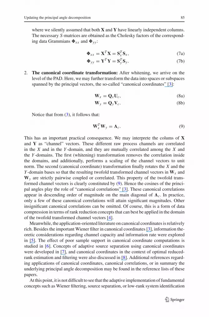
where we silently assumed that both X and Y have linearly independent columns.The necessary S-matrices are obtained as the Cholesky factors of the correspond-ing data Grammians �xx and �yy :

�xx = XT X = STx Sx , (7a)

�yy = YT Y = STy Sy . (7b)

2. The canonical coordinate transformation: After whitening, we arrive on thelevel of the PAD. Here, we may further transform the data into spaces or subspacesspanned by the principal vectors, the so-called “canonical coordinates” [3]:

Wx = Qx Uc, (8a)

Wy = QyVc. (8b)

Notice that from (3), it follows that:

WTx Wy = �c. (9)

This has an important practical consequence. We may interprete the colums of Xand Y as “channel” vectors. These different raw process channels are correlatedin the X and in the Y -domain, and they are mutually correlated among the X andthe Y -domains. The first (whitening) transformation removes the correlation insidethe domains, and additionally, performs a scaling of the channel vectors to unitnorm. The second (canonical coordinate) transformation finally rotates the X and theY -domain bases so that the resulting twofold transformed channel vectors in Wx andWy are strictly pairwise coupled or correlated. This property of the twofold trans-formed channel vectors is clearly constituted by (9). Hence the cosines of the princi-pal angles play the role of “canonical correlations” [3]. These canonical correlationsappear in descending order of magnitude on the main diagonal of �c. In practice,only a few of these canonical correlations will attain significant magnitudes. Otherinsignificant canonical correlations can be omitted. Of course, this is a form of datacompression in terms of rank reduction concepts that can best be applied in the domainof the twofold transformed channel vectors [4].

Meanwhile, the application-oriented literature on canonical coordinates is relativelyrich. Besides the important Wiener filter in canonical coordinates [3], information the-oretic considerations regarding channel capacity and information rate were exploredin [5]. The effect of poor sample support in canonical coordinate computations isstudied in [6]. Concepts of adaptive source separation using canonical coordinateswere developed in [7], and canonical coordinates in the context of optimal reduced-rank estimation and filtering were also discussed in [8]. Additional references regard-ing applications of canonical coordinates, canonical correlations, or in summary theunderlying principal angle decomposition may be found in the reference lists of thesepapers.

At this point, it is not difficult to see that the adaptive implementation of fundamentalconcepts such as Wiener filtering, source separation, or low-rank system identification

123

86 P. Strobach

in canonical coordinates becomes a pressing issue. This leads to the central problemof updating or tracking a principal angle decomposition. Approaches in this directioncan be found already in the application-oriented literature on this topic, such as [9,10].We may realize, however, that the clean updating of a principal angle decompositionin time is a stumbling block that has not been solved satisfactorily until now. Thecurrently existing approaches must be regarded suboptimal as long as they rely ona direct time-updating of correlation matrices, such as �xx , �yy , or �xy . They arefurther regarded suboptimal if deflation strategies are used, because power iterationcombined with deflation is conceptually too serial and will always be outperformedby simultaneous iteration.

In this paper, we are now in a position to solve the principal angle decompositionupdating problem in a competitive fashion. In Sect. 2, we introduce a method thatreceives at its inputs the process snapshot vectors x(t) and y(t), which are usuallyused to update the underlying correlation matrices according to:

�xx (t) = α�xx (t − 1) + x(t)xT (t), (10a)

�yy(t) = α�yy(t − 1) + y(t)yT (t), (10b)

�xy(t) = α�xy(t − 1) + x(t)yT (t), (10c)

where α is a positive exponential forgetting factor close to one. Instead of forming thesematrices explicitly, we introduce a technique that computes the three essential com-ponents Sx (t), Sy(t), and Cxy(t) simultaneously from the input data vectors. Clearly,this will be a square-root method, as it operates directly on the Cholesky-factors ofthe correlation matrices and produces the updated coherence matrix as a “byproduct”.This way, the complete adaptive coherence decomposition can be computed with asingle closed-form recursive algorithm. Once the coherence matrix is available, itpresents no difficulty to track the corresponding SVD as given in (3), namely the coreof the principal angle decomposition. This is shown in Sect. 5. Section 6 presents someinstructive computer experiments with the new algorithm. As a practical example, weshow results of a low-rank system identification experiment in canonical coordinates,a solution that is not widely discussed but appears quite naturally from the modelassumptions underlying the canonical coordinates. Section 7 concludes this paper.

2 Updating the coherence decomposition: basic concept

The updating of the CD is a fundamental preprocessing step in the updating of the PAD.The approach presented here is based on row-Householder reductions for updatingQS-decompositions. The basic recursions are summarized in a complete psuedocodeat the end of this section.

Begin with the definition of the updated process matrices as follows:

X(t) =[

α1/2X(t − 1)

xT (t)

], (11a)

123

Updating the principal angle decomposition 87

Y(t) =[

α1/2Y(t − 1)

yT (t)

]. (11b)

Process matrices in consecutive time steps are posed in terms of their QS-decom-positions:

X(t − 1) = Qx (t − 1)Sx (t − 1), (12a)

Y(t − 1) = Qy(t − 1)Sy(t − 1), (12b)

X(t) = Qx (t)Sx (t), (13a)

Y(t) = Qy(t)Sy(t). (13b)

Clearly, the goal is the direct updating of these QS-decompositions. This can be accom-plished by using the row-Householder reduction [11], a suitable method for solvingrow-oriented updating problems. For instance, a new class of fast subspace trackersbased on the row-Householder reduction has been introduced recently [12,13].

Now consider the direct updating of the QS-decomposition of the X -matrix. Thefollowing scheme can be established:

X(t) =

⎡⎢⎢⎢⎣

0

Qx (t − 1)...

00 · · · 0 1

⎤⎥⎥⎥⎦ Hx (t)Hx (t)

[α1/2Sx (t − 1)

xT (t)

]. (14)

Split (14) into the following recursions:

[Sx (t)0 · · · 0

]= Hx (t)

[α1/2Sx (t − 1)

xT (t)

], (15a)

[Qx (t) qx (t)

] =

⎡⎢⎢⎢⎣

0

Qx (t − 1)...

00 · · · 0 1

⎤⎥⎥⎥⎦ Hx (t). (15b)

Clearly, the goal is the design of a Householder refector Hx (t) that annihilates thebottom row of the appended S-matrix in (15a). In the same fashion, the Y -updatingproblem is formulated:

Y(t) =

⎡⎢⎢⎢⎣

0

Qy(t − 1)...

00 · · · 0 1

⎤⎥⎥⎥⎦ Hy(t)Hy(t)

[α1/2Sy(t − 1)

yT (t)

], (16)

123

88 P. Strobach

where the following recursions are obtained:

[Sy(t)0 · · · 0

]= Hy(t)

[α1/2Sy(t − 1)

yT (t)

], (17a)

[Qy(t) qy(t)

] =

⎡⎢⎢⎢⎣

0

Qy(t − 1)...

00 · · · 0 1

⎤⎥⎥⎥⎦ Hy(t). (17b)

Again, the goal is the annihilation of the bottom row of the appended S-matrix in (17a)by an appropriate row-Householder reflector Hy(t). This is a prototype scenario thatappears freqently in updating problems of this kind, for instance, in subspace tracking.Look up [12] for a detailed discussion. We summarize the main results here, for easyreference.

Suppose we have given an appended S-matrix whose bottom row vector should beannihilated by a row-Householder reduction:

[S′

0 · · · 0

]= H

[SzT

], (18)

where both S and S′ are square matrices of any desired dimension. This annihilationrequires that the Householder reflector

H = I − 2vvT , (19)

where

v =[

vϕ

], (20)

with properties vT v = 1 and HH = I is adjusted according to the following designrule (see [12] for details):

ST b = z −→ b (21a)

β = 4(

bT b + 1)

(21b)

ϕ2 = 1

2+ 1√

β(21c)

v = 1 − 2ϕ2

2ϕb (21d)

Here (21a) denotes an exactly determined system of linear equations that is solvedfor b. Moreover, we shall derive a compact expression for S′. Recall the discussion in

123

Updating the principal angle decomposition 89

[13] and verify that S′ is conveniently obtained as a rank-one updated version of S:

S′ = S − 1

ϕvzT . (22)

This applies directly to the updating problems (15a) and (17a). Before we summarizethe corresponding recursions, consider (15b) and (17b). Clearly, the vertical dimensionof these updated Q-matrices will grow to infinity with time. On the other hand, we arenot interested in the Q-matrices, but only in the Q-Grammian, namely, the coherencemarix Cxy(t), as defined in (3). It is not difficult to see that a recursion for this coherencematrix can be obtained by combining (15b) and (17b) in the following way:

[QT

x (t)qT

x (t)

] [Qy(t) qy(t)

] =[

Cxy(t) QTx (t)qy(t)

qTx (t)Qy(t) qT

x (t)qy(t)

]

= Hx (t)

⎡⎢⎢⎢⎣

0

Cxy(t − 1)...

00 · · · 0 1

⎤⎥⎥⎥⎦ Hy(t). (23)

Notice that in this recursion, only the “new” coherence matrix Cxy(t) at time t mustbe computed explicitly. Hence, we deduce from (23) the following recursion:

Cxy(t) =⎡⎢⎣

0

I...

0

⎤⎥⎦ Hx (t)

⎡⎢⎢⎢⎣

0

Cxy(t − 1)...

00 · · · 0 1

⎤⎥⎥⎥⎦ Hy(t)

[I

0 · · · 0

]. (24)

This constitutes a landmark result. We obtain the “new” coherence matrix Cxy(t)at time t by two-sided row-Householder transformation of the “old” coherence matrixCxy(t − 1) at time t − 1 that appears in a simple augmented form on the right sideof (24). Hence the complete algorithm for a closed-form recursive time-updating ofthe CD is already complete and is constituted by the two recursions (15a) and (17a)for Cholesky factor updating using directly the incoming data snapshot vectors, andrecursion (24) for direct updating of the associated coherence matrix.

All that remains is to write down the equations that determine the two Householderreflectors on which this scheme is founded, and to “streamline” the resulting equationsa little for easy programming. Using the prototype solution (19)–(22), the necessaryrelations can be established as follows:

Hx (t) = I − 2vx (t)vTx (t), (25)

where

vx (t) =[

vx (t)ϕx (t)

], (26)

123

90 P. Strobach

with:

α1/2STx (t − 1)bx (t) = x(t) −→ bx (t) (27a)

βx (t) = 4(

bTx (t)bx (t) + 1

)(27b)

ϕ2x (t) = 1

2+ 1√

βx (t)(27c)

vx (t) = 1 − 2ϕ2x (t)

2ϕx (t)bx (t) (27d)

and

Sx (t) = α1/2Sx (t − 1) − 1

ϕx (t)vx (t)xT (t). (28)

In the same fashion, write:

Hy(t) = I − 2vy(t)vTy (t), (29)

where

vy(t) =[

vy(t)ϕy(t)

], (30)

with:

α1/2STy (t − 1)by(t) = y(t) −→ by(t) (31a)

βy(t) = 4(

bTy (t)by(t) + 1

)(31b)

ϕ2y(t) = 1

2+ 1√

βy(t)(31c)

vy(t) = 1 − 2ϕ2y(t)

2ϕy(t)by(t) (31d)

and

Sy(t) = α1/2Sy(t − 1) − 1

ϕy(t)vy(t)yT (t). (32)

123

Updating the principal angle decomposition 91

All that remains is the explicit evaluation of recursion (24). This requires that wesubstitute the Householder reflectors, as defined in (25), (26), and (29), (30), into (24).After some algebra, it turns out that the coherence matrix is updated as follows:

Cxy(t) = Cxy(t − 1) − 2vx (t)wTx (t) + f(t)vT

y (t), (33)

where

wx (t) = CTxy(t − 1)vx (t), (34a)

wy(t) = Cxy(t − 1)vy(t), (34b)

and

f(t) = γ (t)vx (t) − 2wy(t), (35)

where

γ (t) = 4[vT

x (t)wy(t) + ϕx (t)ϕy(t)]. (36)

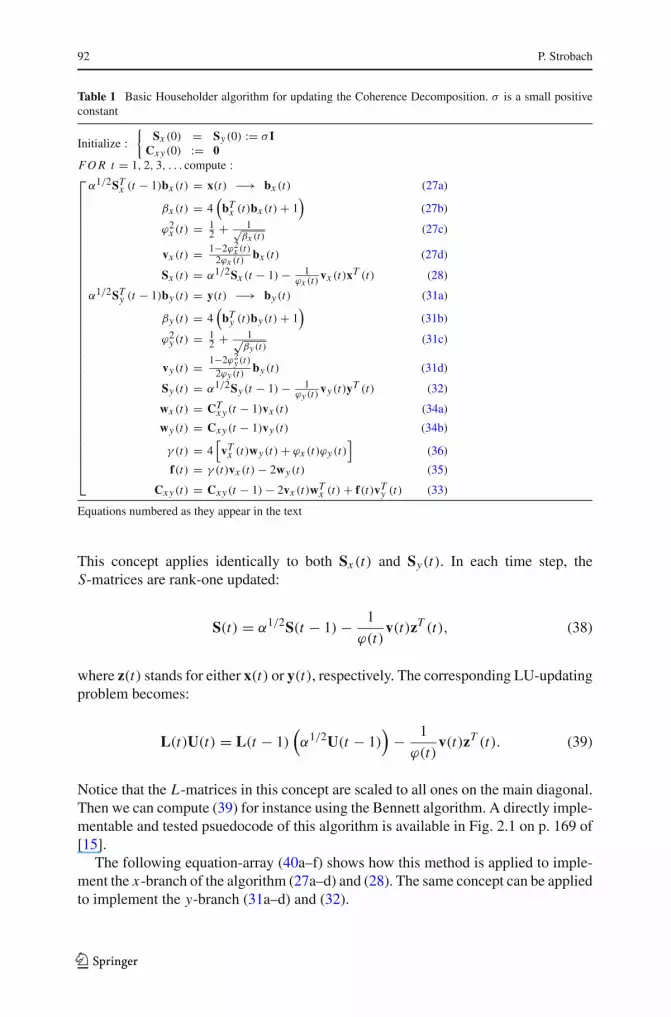
Table 1 shows a complete psuedocode listing of this “raw” form of a direct CD updatingalgorithm or a CD tracker. We can see that in this form, the algorithm is still toodemanding computationally, because it requires the solution of two “large” systemsof linear equations (27a) and (31a) in each time step. On the other hand, the systemmatrices in (27a) and (31a) are rank-one updated in each time step according to (28)and (32). Consequently, the development of fast solutions for a problem of this kindis a standard exercise. In the next Section, we shall examine two concepts, namely: Afirst algorithm based on efficient recursive LU-factor updating [14,15], and a secondalgorithm based on the Matrix Inversion Lemma (Sherman–Morrison Identity) [16].

3 Fast full-rank CD updating algorithms

We present two concepts to exploit the recursivity that is available in the basic CDupdating algorithm of Table 1.

3.1 A CD tracker based on fast LU-factor updating

Suppose that the S-matrices in the algorithm of Table 1 are posed in terms of their LUfactors as follows:

S(t) = L(t)U(t). (37)

123

92 P. Strobach

Table 1 Basic Householder algorithm for updating the Coherence Decomposition. σ is a small positiveconstant

Initialize :{

Sx (0) = Sy(0) := σ ICxy(0) := 0

F O R t = 1, 2, 3, . . . compute :⎡⎢⎢⎢⎢⎢⎢⎢⎢⎢⎢⎢⎢⎢⎢⎢⎢⎢⎢⎢⎢⎢⎢⎢⎢⎢⎢⎢⎢⎢⎢⎢⎢⎢⎢⎢⎢⎢⎣

α1/2STx (t − 1)bx (t) = x(t) −→ bx (t) (27a)

βx (t) = 4(

bTx (t)bx (t) + 1

)(27b)

ϕ2x (t) = 1

2 + 1√βx (t)

(27c)

vx (t) = 1−2ϕ2x (t)

2ϕx (t) bx (t) (27d)

Sx (t) = α1/2Sx (t − 1) − 1ϕx (t) vx (t)xT (t) (28)

α1/2STy (t − 1)by(t) = y(t) −→ by(t) (31a)

βy(t) = 4(

bTy (t)by(t) + 1

)(31b)

ϕ2y(t) = 1

2 + 1√βy (t)

(31c)

vy(t) = 1−2ϕ2y (t)

2ϕy (t) by(t) (31d)

Sy(t) = α1/2Sy(t − 1) − 1ϕy (t) vy(t)yT (t) (32)

wx (t) = CTxy(t − 1)vx (t) (34a)

wy(t) = Cxy(t − 1)vy(t) (34b)

γ (t) = 4[vT

x (t)wy(t) + ϕx (t)ϕy(t)]

(36)

f(t) = γ (t)vx (t) − 2wy(t) (35)

Cxy(t) = Cxy(t − 1) − 2vx (t)wTx (t) + f(t)vT

y (t) (33)

Equations numbered as they appear in the text

This concept applies identically to both Sx (t) and Sy(t). In each time step, theS-matrices are rank-one updated:

S(t) = α1/2S(t − 1) − 1

ϕ(t)v(t)zT (t), (38)

where z(t) stands for either x(t) or y(t), respectively. The corresponding LU-updatingproblem becomes:

L(t)U(t) = L(t − 1)(α1/2U(t − 1)

)− 1

ϕ(t)v(t)zT (t). (39)

Notice that the L-matrices in this concept are scaled to all ones on the main diagonal.Then we can compute (39) for instance using the Bennett algorithm. A directly imple-mentable and tested psuedocode of this algorithm is available in Fig. 2.1 on p. 169 of[15].

The following equation-array (40a–f) shows how this method is applied to imple-ment the x-branch of the algorithm (27a–d) and (28). The same concept can be appliedto implement the y-branch (31a–d) and (32).

123

Updating the principal angle decomposition 93

α1/2UTx (t − 1)dx (t) = x(t) −→ dx (t) (40a)

LTx (t − 1)bx (t) = d(t) −→ bx (t) (40b)

βx (t) = 4(

bTx (t)bx (t) + 1

)(40c)

ϕ2x (t) = 1

2+ 1√

βx (t)(40d)

vx (t) = 1 − 2ϕ2x (t)

2ϕx (t)bx (t) (40e)

Lx (t)Ux (t) = Lx (t − 1)(α1/2Ux (t − 1)

)− 1

ϕx (t)vx (t)xT (t)

(40f)

Initialize this algorithm with L(0) = I and U(0) = σ I, where σ is again a smallpositive start-up constant.

3.2 A CD tracker based on inverse matrix updating

The application of the Matrix Inversion Lemma appears justified in this case, becausethe S-matrices are Cholesky factors of power matrices and hence behave more pleasantin terms of their dynamic range requirements. The resulting algorithm has much incommon with classical recursive least-squares (RLS) concepts [16] and its derivationshould appear rather familiar to those who are familiar with RLS.

Instead of updating the S-matrix, this concept is based on an updating of the cor-responding inverse S-matrix, namely:

P(t) = S−1(t). (41)

Again, we refer to the prototype problem (38), where z(t) stands for either x(t) or y(t),respectively. Hence the solution to this prototype problem applies equally to both xand y-branches of the algorithm. Notice that the system

α1/2ST (t − 1)b(t) = z(t) (42)

can be solved conveniently using the updated inverse as follows:

b(t) = α−1/2PT (t − 1)z(t). (43)

Now evaluate:

P(t) =[α1/2S(t − 1) − 1

ϕ(t)v(t)zT (t)

]−1

. (44)

123

94 P. Strobach

Clearly, this is a case for the classical Matrix Inversion Lemma of the form:

(D + BC)−1 = D−1 − D−1B(

I + CD−1B)−1

CD−1. (45)

Set D = α1/2S(t − 1). Then D−1 = α−1/2P(t − 1). Moreover, set B = − 1ϕ(t)v(t) and

C = zT (t) to obtain:

P(t) = α−1/2P(t − 1) + 1

k(t)p(t)bT (t), (46)

where

p(t) = α−1/2P(t − 1)v(t), (47a)

k(t) = ϕ(t) − bT (t)v(t). (47b)

Table 2 is a complete psuedocode of a fast algorithm for CD tracking based on theupdating of the P-matrix.

Note that the S-matrices are not updated by this algorithm anymore. If one or bothS-matrices are required in a specific application, then it must be updated separatelyusing recursions (28) and/or (32). These recursions can be operated independently. Acase of this kind appears in the experimental Section.

A remark about our experiences with the numerical behavior of this RLS-type CDtracker in comparison with the LU-type CD tracker seems to be in order. We imple-mented the two methods in a problem of dimensions N = 32 and M = 32. Seethe experimental Section for details. The LU-variant of the algorithm showed seri-ous problems in terms of numerical sensitivity when operated under standard singleprecision F90. We observed repeated sudden “outliers” in the variables of this algo-rithm. This was attributed to a loss of significant mantissa digits at some places in thecomputations. In particular, the forward/backsubstitution part (40a,b) of the algorithmrequires double precision arithmetic. Additionally, the Bennett recursions (Fig. 2.1on p. 169 of [15]) had to be implemented in double precision arithmetic for correctoperation. On the other hand, The RLS-variant of the algorithm as displayed in Table 2has been operated without any problems under standard single precision arithmetic inthe same N = 32 and M = 32 application. The problems with the LU-type algorithmare probably curable by appropriate pivoting strategies as discussed in [15]. A detailedinvestigation of this subject exceeds the scope of this paper. In summary, we observeda surprisingly uncritical behavior of the RLS-type CD tracker of Table 2 in all ourexperiments.

4 Low-rank CD tracking

Until now, we have only investigated the case where both �xx (t) and �yy(t) arefull rank. It is not unusual, however, that these matrices are rank-deficient, or may be

123

Updating the principal angle decomposition 95

Table 2 Fast RLS-type Householder algorithm for updating the Coherence Decomposition. σ is a smallpositive constant

Initialize :{

Px (0) = Py(0) := σ−1ICxy(0) := 0

F O R t = 1, 2, 3, . . . compute :⎡⎢⎢⎢⎢⎢⎢⎢⎢⎢⎢⎢⎢⎢⎢⎢⎢⎢⎢⎢⎢⎢⎢⎢⎢⎢⎢⎢⎢⎢⎢⎢⎢⎢⎢⎢⎢⎢⎢⎢⎢⎢⎢⎢⎢⎢⎢⎢⎢⎢⎣

bx (t) = α−1/2PTx (t − 1)x(t) (43)

βx (t) = 4(

bTx (t)bx (t) + 1

)(27b)

ϕ2x (t) = 1

2 + 1√βx (t)

(27c)

vx (t) = 1−2ϕ2x (t)

2ϕx (t) bx (t) (27d)

px (t) = α−1/2Px (t − 1)vx (t) (47a)

kx (t) = ϕx (t) − bTx (t)vx (t) (47b)

Px (t) = α−1/2Px (t − 1) + 1kx (t) px (t)bT

x (t) (46)

by(t) = α−1/2PTy (t − 1)y(t) (43)

βy(t) = 4(

bTy (t)by(t) + 1

)(31b)

ϕ2y(t) = 1

2 + 1√βy (t)

(31c)

vy(t) = 1−2ϕ2y (t)

2ϕy (t) by(t) (31d)

py(t) = α−1/2Py(t − 1)vy(t) (47a)

ky(t) = ϕy(t) − bTy (t)vy(t) (47b)

Py(t) = α−1/2Py(t − 1) + 1ky (t) py(t)bT

y (t) (46)

wx (t) = CTxy(t − 1)vx (t) (34a)

wy(t) = Cxy(t − 1)vy(t) (34b)

γ (t) = 4[vT

x (t)wy(t) + ϕx (t)ϕy(t)]

(36)

f(t) = γ (t)vx (t) − 2wy(t) (35)

Cxy(t) = Cxy(t − 1) − 2vx (t)wTx (t) + f(t)vT

y (t) (33)

Equations numbered as they appear in the text

reduced in rank because the information of interest in these matrices can be representedin subspaces of lower or much lower dimensions. Situations of this kind occur typicallyin cases, where addititive noise comes into the play. This noise maintains the full rankof the associated matrices, but still the information of interest can be mapped intosubspaces of lower or much lower dimensions. See also the experimental Section,where we present a case of this kind. In such cases, the application of rank reductiontechniques to one or both inputs kills two flies with one blow: The overall noise levelon the specific input is decreased, but most importantly, the overall operations countcan be decreased drastically.

The next question is how rank reduction can be incorporated in the CD track-ing problem. For this purpose, we recall the updating structures of the full-rankQS-decompositions of the X and Y -data matrices according to (14) and (16). Rankreduction means that we substitute these data matrices by approximants of lowerrank as follows:

123

96 P. Strobach

X(t) ≈ Xn(t) = Qx,n(t)Sx,n(t) n < N , (48a)

Y(t) ≈ Ym(t) = Qy,m(t)Sy,m(t) m < M, (48b)

where n and m are the reduced ranks of the x and y-channels, respectively. Conse-quently, Sx,n(t) is a rectangular n × N matrix and Sy,m(t) is a rectangular m × Mmatrix. In the full-rank case, the new (incoming) data snapshots are mapped into thedecompositions of the next time step according to (14) and (16). In the same fashion,the accomodation of new snapshots in case of the above approximants can be posedas follows:

Xn(t) + �x,n(t) =

⎡⎢⎢⎢⎣

0

Qx,n(t − 1)...

00 · · · 0 1

⎤⎥⎥⎥⎦ Hx,n(t)Hx,n(t)

[α1/2Sx,n(t − 1)

xT (t)

], (49)

Ym(t) + �y,m(t) =

⎡⎢⎢⎢⎣

0

Qy,m(t − 1)...

00 · · · 0 1

⎤⎥⎥⎥⎦ Hy,m(t)Hy,m(t)

[α1/2Sy,m(t − 1)

yT (t)

],

(50)

where the ∆-matrices denote rank-one layers representing the inevitable rank-increasecaused by updating. Since these rank-one layers are omitted from one time step to thenext, the accomodation of the incoming data snapshot is optimal, if the power ofthese rank-one layers is minimized. This is achieved by an appropriate design of thereduced Householder matrices Hx,n(t) and Hy,m(t). Consider the following updatingrecursions:

[Sx,n(t)εT

x (t)

]= Hx,n(t)

[α1/2Sx,n(t − 1)

xT (t)

], (51a)

[Sy,m(t)εT

y (t)

]= Hy,m(t)

[α1/2Sy,m(t − 1)

yT (t)

]. (51b)

Clearly, these updating recursions are just the rank-reduced counterparts of (15a) and(17a): We realize that the key difference between these recursions and their correspond-ing full-rank predecessors is that now, we are facing overdetermined row-Householderreduction problems here. The Householder reflectors Hx,n(t) and Hy,m(t) must bedesigned so that the error vectors εT

x (t) and εTy (t) are minimized in some sense.

Since all further considerations on this subject are absolutely identical for the xand y-channels, we streamline the presentation a little in that in the following, allx and y-related variables are represented by z and the subscripts are generally omitted.Hence the prototype overdetermined row-Householder reduction problem becomes:

[S(t)εT (t)

]= H(t)

[α1/2S(t − 1)

zT (t)

], (52)

123

Updating the principal angle decomposition 97

and the Q-update can be posed as follows:

[Q(t) q(t)

] =

⎡⎢⎢⎢⎣

0

Q(t − 1)...

00 · · · 0 1

⎤⎥⎥⎥⎦ H(t). (53)

Consequently, we can write:

Z(t) + �(t) = [Q(t) q(t)

] [S(t)εT (t)

]

= Q(t)S(t) + q(t)εT (t). (54)

From this equation, it follows that:

Z(t) = Q(t)S(t), (55)

and

�(t) = q(t)εT (t). (56)

This, in turn, reveals that:

tr{�T (t)�(t)} = εT (t)ε(t) = E(t). (57)

Hence a minimization of the error vector directly minimizes the rank-one residuallayer that is dumped after each time update. The following observations can be made:

1. We are confronted with a formidable optimization problem E(t)!= min here.

2. Based on the solution of this optimization problem, we effectively establish thebasis for a new family of subspace trackers, namely, the square-root Householdersubspace trackers [17]. To see this, consider the approximant of the correspondingcovariance matrix:

�zz(t) ≈ �zz(t) = ZT (t)Z(t) = ST (t)S(t). (58)

Assume any kind of orthonormal decomposition of ST (t), for instance, a QR-decomposition for the moment:

ST (t) = Qs(t)Rs(t) : QR-factorization. (59)

Then we can write:

�zz(t) = Qs(t)Rs(t)RTs (t)QT

s (t)

= V(t)�(t)VT (t), (60)

123

98 P. Strobach

where V(t) is the matrix of estimated leading (n or m) eigenvectors of �zz(t)and �(t) is the corresponding diagonal matrix of estimated dominant or leadingeigenvalues. Clearly, these estimated eigenvalues are orthonormally similar to theproduct Rs(t)RT

s (t):

�(t) = �(t)Rs(t)RTs (t)�T (t), (61)

where �T (t)�(t) = I represents any suitable orthonormal similarity transfor-mation. Moreover, with the presence of a factorization like Rs(t)RT

s (t), we areeffectively operating on the square-root level, because the diagonal matrix of esti-mated leading singular values of Z(t) is easily established as:

�1/2

(t) = �(t)Rs(t)�T (t), (62)

where �T (t)�(t) = I represents a second suitable orthonormal similarity trans-formation. Finally,

V(t) = Qs(t)�T (t) (63)

can also be regarded as the matrix of estimated leading right singular vectors in theSVD of Z(t). Hence, we have a square-root technique here, and we are effectivelyoperating on Cholesky factors of power matrices like, for instance, Rs(t) or otherfactorizations of this kind. This has its attractions over conventional techniqueslike those described in [12] in terms of dynamic range requirements. Details aboutthis exciting new class of square-root Householder subspace trackers, including

a deeper discussion of the underlying optimization problem E(t)!= min, its fast

sequential solution and maximally fast forms, will be presented in [17].

In this context, here, only the most elementary form of a square-root Householdersubspace tracker is presented and is used for our purpose of low-rank CD tracking. Thisalgorithm is based on a clever strategy for a highly effective approximate minimizationof the criterion E(t). Recall the QR-factorization of the transposed S-matrix as givenin (59). Substitute this decomposition into (52). This yields:

[RT

s (t)QTs (t)

εT (t)

]= H(t)

[α1/2RT

s (t − 1)QTs (t − 1)

zT (t)

]. (64)

Postmultiply both sides of this expression by Qs(t − 1). We obtain:

[RT

s (t)QTs (t)Qs(t − 1)

εT (t)Qs(t − 1)

]= H(t)

[α1/2RT

s (t − 1)

zT (t)Qs(t − 1)

]. (65)

In this expression, we can identify terms which are well-known in the area of subspacetracking [12], namely:

�(t) = QTs (t − 1)Qs(t), (66)

123

Updating the principal angle decomposition 99

and

h(t) = QTs (t − 1)z(t). (67)

Hence, we can write:

[RT

s (t)�T (t)εT (t)Qs(t − 1)

]= H(t)

[α1/2RT

s (t − 1)

hT (t)

]. (68)

Consider the special case that ε(t) is regarded the complement of the orthogonalprojection of a vector onto the subspace spanned by Qs(t − 1). This yields:

εT (t)Qs(t − 1) = [0 · · · 0] . (69)

Clearly, this way the overdetermined Householder problem (52) is converted into anexactly determined row-Householder problem that can be solved conveniently usingthe standard formulas (18)–(21a–d):

α1/2Rs(t − 1)b(t) = h(t) −→ b(t) (70a)

β(t) = 4(

bT (t)b(t) + 1)

(70b)

ϕ2(t) = 1

2+ 1√

β(t)(70c)

v(t) = 1 − 2ϕ2(t)

2ϕ(t)b(t) (70d)

An interpretation of this specific result can be instructive. Recall the definition ofH(t) according to (19) and (20). Then evaluate the bottom row of (64):

ε(t) = −2α1/2ϕ(t)Qs(t − 1)Rs(t − 1)v(t) +(

1 − 2ϕ2(t))

z(t). (71)

Use the special solution (70d) to find:

ε(t) = −α1/2(

1 − 2ϕ2(t))

Qs(t − 1)Rs(t − 1)b(t) +(

1 − 2ϕ2(t))

z(t). (72)

Finally, employ (70a) to obtain:

ε(t) =(

1 − 2ϕ2(t))

[z(t) − Qs(t − 1)h(t)] . (73)

It is commonly known that

z⊥(t) = z(t) − Qs(t − 1)h(t) (74)

123

100 P. Strobach

is just the complement of the orthogonal projection of z(t) onto the subspace spannedby Qs(t − 1). Consequently, ε(t) is just a scaled version thereof. This also means thatH(t) is designed so that all those components of z(t), that can be represented in thesubspace spanned by Qs(t − 1), are mapped into the actual approximant Z(t). Thisis a standard solution known from fast subspace tracking [12]. This solution is verypowerful although it does not solve the underlying minimization problem exactly. Fordetails on this subject, see [17].

Equation-array (75a–g) is a psuedocode of this elementary square-root House-holder subspace tracker for updating the rectangular low-rank Cholesky factor S(t)in time. Initialize this algorithm with Qs(0) := random orthonormal, Rs(0) := σ I,and S(0) = RT

s (0)QTs (0).

h(t) = QTs (t − 1)z(t) (75a)

α1/2Rs(t − 1)b(t) = h(t) −→ b(t) (75b)

β(t) = 4(

bT (t)b(t) + 1)

(75c)

ϕ2(t) = 1

2+ 1√

β(t)(75d)

v(t) = 1 − 2ϕ2(t)

2ϕ(t)b(t) (75e)

S(t) = α1/2[I − 2v(t)vT (t)

]S(t − 1) − 2ϕ(t)v(t)zT (t)

(75f)

ST (t) = Qs(t)Rs(t) : QR-factorization (75g)

Note also that the corresponding Q-update (53) is of course not computed explicitly,because we use H(t) directly for updating of the coherence matrix as outlined in(23). In the case of low-rank updating, the dimension of the coherence matrix reducesaccordingly, from dimension N ×M in the full-rank case to n×m in the two-sided low-rank case. Note, however, that we are completely free in the choice of the processingconcepts for the individual channels. Even mixed configurations are possible. Forinstance, we could work with the RLS-type full-rank Householder algorithm of Table 2in the x-branch of the algorithm, while the y-branch is processed using the low-rankalgorithm of equation-array (75a–g). In the simulation Section, such a mixed algorithmis studied experimentally.

5 Tracking the SVD of the coherence matrix

A final step is the tracking of the singular values and vectors of the coherence matrix orequivalently, the cosines of the principal angles and the associated principal vectors.In practice, only a few (r < min{n, m}) singular values and vectors are computed.

123

Updating the principal angle decomposition 101

This is accomplished using a standard bi-iteration [13]. This bi-iteration is constitutedby the following recurrence:

A(t) = Cxy(t)QB(t − 1), (76a)

A(t) = QA(t)RA(t) ; QR-factorization, (76b)

B(t) = CTxy(t)QA(t), (76c)

B(t) = QB(t)RB(t) ; QR-factorization, (76d)

where A(t) is an auxiliary matrix of dimension n × r and B(t) is an auxiliary matrixof dimension m × r in the general case. In the specific case of full-rank channelprocessing, we have n = N and m = M . Observe that the desired low-rank SVDapproximant Cxy(t) of (3) is directly obtained from (76c,d) as follows:

Cxy(t) = QA(t)QTA(t)Cxy(t)

= QA(t)RTB(t)QT

B(t)

= Uc,r (t)�c,r (t)VTc,r (t). (77)

The desired cosines of principal angles �c,r (t) emerge directly on the main diago-nal of RT

B(t). Note this bi-iteration converges very rapidly and accurately in mostpractical cases. Only a single iteration is required in each time step. No furthersimplifications on this routine are recommended in this application. Initialize withQB(0) := random orthonormal, as usual.

6 Low-rank adaptive system identification using the PAD

It remains to demonstrate the operation and the characteristics of the presented algo-rithms in terms of some instructive computer experiments. For this purpose, we studya low-rank system identification problem of the following kind:

s(t) = FT (t)x(t), (78a)

y(t) = s(t) + n(t), (78b)

where x(t) is an excitation vector of N statistically independent Gaussian randomvariables, n(t) is a dimension M vector of white Gaussian noise, and y(t) is an obser-vation vector of dimension M . F(t) is a system matrix of dimension N × M . The goalis the on-line sequential identification of F(t) based on the observed input x(t) andoutput y(t) snapshots.

An estimate F(t) of the system matrix can be obtained on the basis of the presentand the past observations of the observed processes and is hence constituted as follows,

Y(t) = X(t)F(t) + N(t), (79)

where X(t) and Y(t) are exponentially stacked observations as defined in (11a,b), andN(t) accomodates noise and fitting errors.

123

102 P. Strobach

The desired estimate F(t) of the system matrix can be calculated, if the followingassumption holds:

XT (t)N(t) = 0. (80)

In this case, we premultiply (79) by XT (t) and obtain:

XT (t)Y(t) = XT (t)X(t)F(t), (81)

or equivalently,

F(t) = �−1xx (t)�xy(t), (82)

where we used the definitions (10a–c). The direct calculation of F(t) using (82) isnot wise, particularly in cases where this system matrix obeys a low-rank represen-tation. In such cases, the method of canonical coordinates using the elements of theprincipal angle decomposition (PAD) is the preferable method. Hence, we considerthe factorized representation of �xx (t), and the updated PAD of �xy(t) as follows:

�xx (t) = STx (t)Sx (t) → �−1

xx (t) = S−1x (t)S−T

x (t), (83)

�xy(t) = STx (t)QA(t)RT

B(t)QTB(t)Sy(t). (84)

Finally, recall (41) to obtain the following PAD-based identification formula:

F(t) = Px (t)QA(t)RTB(t)QT

B(t)Sy(t). (85)

We can see that this formula is completely amenable to rank-reduction strategies. Forinstance, we can immediately see that in the case of vanishing noise, the rank of theoutput covariance matrix is equal the rank of the matrix to be identified:

rank{�yy(t)} = rank{F(t)}. (86)

Hence, we shall first apply a rank-reduction to the y-inputs in the case of a low-rank system matrix. Secondly, the estimated cosines of principal angles on the maindiagonal of RB(t) will exhibit the dimensionality or the rank of the system matrixto be identified. This is particularly convenient, because these cosines of principalangles are always positive and scaled to values of less or equal one. Hence, we canapply a fixed thresholding operation here, and estimate the rank adaptively. Only thosecomponents whose associated cosines of principal angles exceed a certain threshold,are used in the construction of the estimated F(t). Hence, we have here a very reliablemethod for rank-adaptive processing, because cosines of principal angles are scaledquantities by definition.

Moreover, it is important to realize that this PAD-based identification according to(85) is an all square-root method. No power or crosscorrelation matrices are updatedexplicitly anymore. The necessary Cholesky factors are directly computed from theincoming data using the new CD trackers.

123

Updating the principal angle decomposition 103

6.1 The experimental setup

The PAD-based on-line system identifier (85) has been tested experimentally. In theexperiments to be shown in the sequel, we operated the system model (78a,b) withdimensions N = 32 and M = 32, respectively. Throughout all experiments, theexponential forgetting factor was fixed at a value of α = 0.994. Each experimentcomprises 10 statistically independent trial runs of at least 6,000 time steps per trialrun. Each trial run comprises two stationary regions in which the system matrix is fixed.In the first interval 0 ≤ t ≤ 3, 000, a system matrix F1 with elements F1(i, j), 1 ≤i ≤ N , 1 ≤ j ≤ M, is used. These matrix elements are determined as follows:

F1(i, j) = 0.95i 0.90 j sin(π

6i)

cos(π

4j)

. (87)

This is clearly a rank-one matrix. In the second interval t > 3, 000, we used a systemmatrix F2 of the same dimension with elements:

F2(i, j)=0.85i 0.96 j cos(π

3i)

sin(π

5j)+0.98i 0.89 j sin

( π

10i)

cos(π

8j)

. (88)

This is clearly a rank-two matrix. All experiments were carried out at an SNR (signal-to-noise-ratio) of+6 dB. The SNR is defined as follows:

SNR = 10 log10

(Ps

Pn

), (89)

where

Ps =∑

sT (t)s(t), (90a)

Pn =∑

nT (t)n(t), (90b)

where the summation comprises all time steps in all the 10 independent trial runs.

6.2 The experiments

In a first experiment, we verify the operation of the RLS-type Householder CD trackerof Table 2. Together with this algorithm, we operated the recursions (28) and (32) forupdating the full-rank Cholesky factors Sx (t) and Sy(t). Additionally, the underlyingcorrelation matrices (10a–c) were computed explicitly, as a reference.

For evaluation of the Cholesky factors, the following error matrices were computed:

Exx (t) = �xx (t) − STx (t)Sx (t), (91a)

Eyy(t) = �yy(t) − STy (t)Sy(t). (91b)

123

104 P. Strobach

Recall the definition of the Cholesky factors according to (7a,b). These error matricesreveal the quality of the estimated Cholesky factors in comparison with the explicitlytracked reference matrices. The following log-distances were computed:

exx (t) = 10 log10

(tr{ET

xx (t)Exx (t)})

[d B], (92a)

eyy(t) = 10 log10

(tr{ET

yy(t)Eyy(t)})

[d B]. (92b)

Figure 1 shows the criterion exx (t) displayed for the 10 independent trial runs. Figure 2shows the criterion eyy(t). We can see, these tracked Cholesky factors match with theunderlying matrices up to machine accuracy.

-70

-60

-50

-40

-30

-20

-10

0

0 1000 2000 3000 4000 5000 6000

x-co

varia

nce

squa

re-r

oot f

ittin

g er

ror

[dB

]

discrete time

Fig. 1 x-covariance square-root fitting error of 10 independent trial runs plotted in one diagram

-70

-60

-50

-40

-30

-20

-10

0

0 1000 2000 3000 4000 5000 6000

y-co

varia

nce

squa

re-r

oot f

ittin

g er

ror

[dB

]

discrete time

Fig. 2 y-covariance square-root fitting error of 10 independent trial runs plotted in one diagram

123

Updating the principal angle decomposition 105

A next concern is the test of the coherence matrix. For this purpose, we computedthe so-called CD fitting error as follows:

Exy(t) = �xy(t) − STx (t)Cxy(t)Sy(t). (93)

This error matrix monitors the complete CD and hereby implicitly the quality of thecoherence matrix Cxy(t), because the quality of the Cholesky factors has already beenverified. The following log-distance is computed:

exy(t) = 10 log10

(tr{ET

xy(t)Exy(t)})

[d B]. (94)

Figure 3 shows the tracks of this CD fitting error for the 10 independent trial runs. Thistest confirms that the algorithm can track the CD correctly up to machine accuracy.

Now we should have a look at the singular values of the coherence matrix, alsoknown as the cosines of the principal angles. For this purpose, the bi-iteration (76a–d)has been operated with a fixed rank of r = 4. We plotted the main diagonal elementsof RB(t), or equivalently, the cosines of the principal angles, averaged over all the 10independent trial runs, in Fig. 4. We can see that in the first section 0 ≤ t ≤ 3, 000,there exists one dominant singular value that approaches almost perfectly the topvalue of 1. The other three remaining singular values are clearly subdominant. Theyrepresent the noise while the dominant singular value indicates that the system matrixto be identified is a rank-one matrix. The situation changes after t = 3, 000. Herewe can see, that a second singular value becomes dominant. This indicates that thesystem matrix to be identified has changed to a rank-two matrix while the noise levelremained unchanged, as expected.

A next issue is the evaluation of the PAD-based identification formula (85) with full-rank Cholesky factors as provided by the CD tracker of Table 2. Hence the necessaryrank reduction is entirely performed on the coherence SVD level. However, we arefaced with a difficulty here: Only the dominant principal angles should be incorporated

-70

-60

-50

-40

-30

-20

-10

0

0 1000 2000 3000 4000 5000 6000

cohe

renc

e de

com

posi

tion

fittin

g er

ror

[dB

]

discrete time

Fig. 3 Coherence decomposition fitting error of 10 independent trial runs plotted in one diagram

123

106 P. Strobach

0

0.2

0.4

0.6

0.8

1

0 1000 2000 3000 4000 5000 6000

cosi

nes

of p

rinci

pal a

ngle

s

discrete time

Fig. 4 Tracks of r = 4 leading cosines of principal angles averaged over 10 independent trial runs

in the calculation of F(t) according to (85). Hence, we should construct the core SVDapproximant QA(t)RT

B(t)QTB(t) in (85) layerwise as follows:

QA(t)RTB(t)QT

B(t) → Cxy(t) =rs (t)∑ρ=1

RB,ρρ(t)qA,ρ(t)qTB,ρ(t), (95)

where rs(t) < r is a variable rank estimate that is calculated in each time step as thenumber of cosines of estimated principal angles RB,ρρ(t) (main diagonal elements ofRB(t)) that exceed a certain fixed threshold τs . We can see from Fig. 4, that determininga threshold value is particularly uncritical here because of the always fixed range of thecosines of principal angles. In our experiment, we choose: τs = 0.7. In (95), qA,ρ(t)and qB,ρ(t) denote the column vectors of QA(t) and QB(t), respectively.

The quality of the estimated system matrix F(t) is monitored in terms of the dis-tances between the estimated and the true system matrices F1 and F2 as follows:

EF1(t) = F1 − F(t), (96a)

EF2(t) = F2 − F(t). (96b)

We plotted the corresponding two log-distances in the diagram of Fig. 5:

eF1(t) = 10 log10

(tr{ET

F1(t)EF1(t)})

[d B], (97a)

eF2(t) = 10 log10

(tr{ET

F2(t)EF2(t)})

[d B]. (97b)

We can see from Fig. 5, that the estimator clearly identifies the system matrices cor-rectly. Figure 6 shows the corresponding tracks of the associated estimated subrank.In the first region 0 ≤ t ≤ 300, the estimator identifies rs(t) = 1 correctly, and in the

123

Updating the principal angle decomposition 107

-20

-15

-10

-5

0

5

10

15

20

0 1000 2000 3000 4000 5000 6000

para

met

er fi

tting

err

or [d

B]

discrete time

Fig. 5 Log-distances between true (F1 and F2) and tracked F(t) model parameter matrices using subrank-adaptive reconstruction with a cosine of principal angle threshold of τs = 0.7. 10 independent trial runs inone diagram

0

0.5

1

1.5

2

2.5

3

3.5

4

0 1000 2000 3000 4000 5000 6000

estim

ated

sub

rank

discrete time

Fig. 6 Estimated subrank rs (t) as a function of time for the adaptive rank reconstruction result as displayedin Fig. 5. Rank tracks of 10 independent trial runs displayed in one diagram

region t > 3, 000, rs(t) = 2 is estimated correctly, as expected from the underlyingcosine of principal angle tracks as displayed in Fig. 4.

Until now, we have not utilized property (86), namely, that the rank of the infor-mation in the y-channel is not larger than the rank of the system matrix. Hence thefull-rank Sy(t) in (85) should be replaceable by a rectangular Cholesky factor withoutany loss in estimation performance. To examine this idea, we replaced the full-rankCholesky factor estimator of the y-channel in the algorithm of Table 2 by the low-rankrectangular Cholesky factor estimator as displayed in equation-array (75a–g). Hereby,we arrive at one of the so-called “mixed” algorithms. Table 3 is an exact psuedocodeof this mixed algorithm that we used here for perfect utilization of the rank propertiesavailable in an identification problem of this kind.

123

108 P. Strobach

Table 3 Mixed x-channel RLS-type Householder and y-channel low-rank rectangular Cholesky factoralgorithm for updating the low-rank Coherence Decomposition. σ is a small positive constant

Initialize :

⎧⎪⎪⎪⎪⎪⎪⎨⎪⎪⎪⎪⎪⎪⎩

Px (0) := σ−1I

Cxy(0) := 0

Rsy(0) := σ I

Qsy(0) : random orthonormal

Sy,m (0) = RTsy(0)QT

sy(0)

F O R t = 1, 2, 3, . . . compute :⎡⎢⎢⎢⎢⎢⎢⎢⎢⎢⎢⎢⎢⎢⎢⎢⎢⎢⎢⎢⎢⎢⎢⎢⎢⎢⎢⎢⎢⎢⎢⎢⎢⎢⎢⎢⎢⎢⎢⎢⎢⎢⎢⎢⎢⎢⎢⎢⎢⎢⎣

bx (t) = α−1/2PTx (t − 1)x(t) (43)

βx (t) = 4(

bTx (t)bx (t) + 1

)(27b)

ϕ2x (t) = 1

2 + 1√βx (t)

(27c)

vx (t) = 1−2ϕ2x (t)

2ϕx (t) bx (t) (27d)

px (t) = α−1/2Px (t − 1)vx (t) (47a)

kx (t) = ϕx (t) − bTx (t)vx (t) (47b)

Px (t) = α−1/2Px (t − 1) + 1kx (t) px (t)bT

x (t) (46)

hy(t) = QTsy(t − 1)y(t) (75a)

α1/2Rsy(t − 1)by(t) = hy(t) −→ by(t) (75b)

βy(t) = 4(

bTy (t)by(t) + 1

)(75c)

ϕ2y(t) = 1

2 + 1√βy (t)

(75d)

vy(t) = 1−2ϕ2y (t)

2ϕy (t) by(t) (75e)

Sy,m (t) = α1/2[I − 2vy(t)vT

y (t)]

Sy,m (t − 1) − 2ϕy(t)vy(t)yT (t) (75f)

STy,m (t) = Qsy(t)Rsy(t) : QR-factorization (75g)

wx (t) = CTxy(t − 1)vx (t) (34a)

wy(t) = Cxy(t − 1)vy(t) (34b)

γ (t) = 4[vT

x (t)wy(t) + ϕx (t)ϕy(t)]

(36)

f(t) = γ (t)vx (t) − 2wy(t) (35)

Cxy(t) = Cxy(t − 1) − 2vx (t)wTx (t) + f(t)vT

y (t) (33)

Equations numbered as they appear in the text

The associated low-rank coherence-based estimator becomes:

Fm(t) = Px (t)QA(t)RTB(t)QT

B(t)Sy,m(t). (98)

In the experiments, the dimension of the “y-bottleneck” was fixed to a value of m = 4.Of course, Cxy(t) reduces accordingly in size to an N ×m matrix and the dimensions ofthe variables in the bi-iteration (76a–d) must be adapted accordingly. Then we obtainfrom this configuration the tracked cosines of principal angles as displayed in Fig. 7.A comparison of these tracks with the corresponding tracks of Fig. 4 in the case of thefull-rank y-channel processing reveals that now, the subdominant cosines of principalangles appear decreased. This is clearly a consequence of the fact that we increased they-input SNR by rank reduction. The information, however, should not suffer from this

123

Updating the principal angle decomposition 109

0

0.2

0.4

0.6

0.8

1

0 1000 2000 3000 4000 5000 6000

cosi

nes

of p

rinci

pal a

ngle

s

discrete time

Fig. 7 Tracks of r = 4 leading cosines of principal angles obtained with y-input rank reduction to m = 4.Average of 10 independent trial runs

rank reduction, because it fits easily through an y-bottleneck of size m = 4. This is alsoconfirmed by comparing the tracks of the dominant cosines in Figs. 4 and 7, which arepractically identical. Hence, we conclude that this rank reduction on the y-inputs hasgiven us an advantage in terms of a reduced computational complexity, but additionally,the disparity of dominant and subdominant cosines has been increased. This makesthresholding one more bit easier and safer. The corresponding log-distances betweenthe true and the estimated system matrix are shown in Fig. 8. A comparison with thesame criterion obtained under full-rank y-processing (Fig. 5) reveals that the estimationresult will not suffer from this y-rank reduction, as expected.

-20

-15

-10

-5

0

5

10

15

20

0 1000 2000 3000 4000 5000 6000

para

met

er fi

tting

err

or [d

B]

discrete time

Fig. 8 Log-distances between true (F1 and F2) and tracked F(t) model parameter matrices using subrank-adaptive reconstruction with a cosine of principal angle threshold of τs = 0.7 and y-input rank reductionto m = 4

123

110 P. Strobach

A final issue is the stability of the proposed algorithms in terms of round-off erroraccumulation or other perturbations that may affect the variables of the algorithmsin sequential operation. Although a thorough study of these aspects clearly exceedsthe scope of this paper, we shall not close this experimental Section without a littleexperiment that reveals much about the nature of the proposed algorithms in termsof these stability issues. If one looks at the algorithm of Table 3, which is the mostsophisticated algorithm of this paper, one may argue that a sudden perturbation ofCxy(t) may cause the most destructive effect to this algorithm. Hence, we repeatedthe experiment of Figs. 7 and 8, and at time t = 5, 000, we added a random pertur-bation matrix � with property tr{�T �} = 1 to Cxy(t = 5, 000), which causes aninstantaneous transient in the results, as is displayed in Figs. 9 and 10. However, it isalso seen that the algorithm stabilizes and returns to normal operation very rapidly.This experiment indicates that the proposed algorithms are completely self-stabilizing.Hence no restarts are necessary in sequential operation, not even in presence of roughperturbations. These algorithms should automatically recover to normal operation inmost cases and they should be immune against any round-off error buildup.

7 Conclusions

It is the purpose of this paper to present a competitive approach to principal angledecomposition tracking, a method that is of key importance in the online processingof correlated vector signals. Our approach emerged as a clear consequence of recentinsights in orthonormal decompositions and strategies for their efficient updating usingthe row-Householder method. Additionally, we layed the foundation of square-rootHouseholder subspace tracking, a very worthwhile new technique, which we neededin our context. An instructive typical application example of principal angle decom-position tracking has been been examined in terms of a low-rank adaptive systemidentification experiment.

0

0.2

0.4

0.6

0.8

1

0 1000 2000 3000 4000 5000 6000 7000 8000

cosi

nes

of p

rinci

pal a

ngle

s

discrete time

Fig. 9 r = 4 leading cosines of principal angles with y-input rank reduction to m = 4 and a suddenperturbation of the coherence matrix at t = 5, 000

123

Updating the principal angle decomposition 111

-20

-15

-10

-5

0

5

10

15

20

0 1000 2000 3000 4000 5000 6000 7000 8000

para

met

er fi

tting

err

or [d

B]

discrete time

Fig. 10 Log-distances between true (F1 and F2) and tracked F(t) model parameter matrices using subrank-adaptive reconstruction with τs = 0.7, y-input rank reduction to m = 4, and a sudden perturbation of thecoherence matrix at t = 5, 000

References

1. Golub, G.H., van Loan, C.F.: Matrix Computations, 2nd edn. John Hopkins University Press,Baltimore (1989)

2. Björck, A., Golub, G.H.: Numerical methods for computing angles between linear subspaces. Math.Comput. 27, 579–594 (1973)

3. Scharf, L.L., Thomas, J.K.: Wiener filters in canonical coordinates for transform coding, filtering,and quantizing. IEEE Trans. Sig. Process. 46(3), 647–653 (1998)

4. Pezeshki, A., Scharf, L.L., Thomas, J.K., van Veen, B.D.: Canonical coordinates are the right coor-dinates for low-rank Gauss-Gauss detection and estimation. IEEE Trans. Sig. Process. 54(12), 4817–4820 (2006)

5. Scharf, L.L., Mullis, C.T.: Canonical coordinates and the geometry of inference, rate, and capac-ity. IEEE Trans. Sig. Process. 48(3), 824–831 (2002)

6. Pezeshki, A., Scharf, L.L., Azimi-Sadjadi, M.R.: Effect of poor sample support on empirical canonicalcorrelations and coordinates. IEEE Trans. Sig. Process., June (2007, review)

7. Schell, S.V., Gardner, W.A.: Programmable canonical correlation analysis: a flexible framework forblind adaptive spatial filtering. IEEE Trans. Sig. Process. 43, 2898–2908 (1995)

8. Hua, Y., Nikpour, M., Stoica, P.: Optimal reduced-rank estimation and filtering. IEEE Trans. Sig.Process. 49, 457–469 (2001)

9. Pezeshki, A., Scharf, L.L., Azimi-Sadjadi, M.R., Hua, Y.: Two-channel constrained least squaresproblems: Solutions using power methods and connections with canonical coordinates. IEEE Trans.Sig. Process. 53, 121–135 (2005)

10. Pezeshki, A., Azimi-Sadjadi, M.R., Scharf, L.L.: A network for recursive exraction of canonicalcoordinates. Neural Netw. 16, 801–808 (2003)

11. Bojanczyk, A.W., Nagy, J.G., Plemmons, R.J.: Block RLS using row Householder reflections. Lin.Alg. Appl. 188, 31–62 (1993)

12. Strobach, P.: The fast recursive row-Householder subspace tracking algorithm. Numer. Math., July(2007, submitted)

13. Strobach, P.: The fast Householder Bi-SVD subspace tracking algorithm. Sig. Process. (2008, in press)14. Bennett, J.: Triangular factors of modified matrices. Numer. Math. 7, 217–221 (1965)15. Stange, P., Griewank, A., Bollhöfer, M.: On the efficient update of rectangular LU-factorizations

subject to low-rank modifications. Electron. Trans. Numer. Anal. 26, 161–177 (2007)

123

112 P. Strobach

16. Strobach, P.: Linear prediction theory: a mathematical basis for adaptive systems. Springer Series inInformation Sciences, vol. 21. Springer, Berlin (1990)

17. Strobach, P.: Square-root Householder subspace tracking. Numer. Math., Sept. (2007, review)

123