i

Centre for Geo-Information

Thesis Report GIRS-2016-04

URBAN HEAT ISLANDS AND URBAN CONFIGURATION

Andrea van Milgen - Kos

25-4

-201

6

ii

iii

URBAN HEAT ISLANDS AND URBAN CONFIGURATION

Andrea van Milgen - Kos

Registration number 89 03 18 469 040

Supervisor:

dr.ir. RJA (Ron) van Lammeren

A thesis submitted in partial fulfilment of the degree of Master of Science

at Wageningen University and Research Centre,

The Netherlands.

25 April 2016

Wageningen, The Netherlands

Thesis code number: GRS-80436 Thesis Report: GIRS-2016 –04 Wageningen University and Research Centre Laboratory of Geo-Information Science and Remote Sensing

iv

v

ABSTRACT Due to continuing urbanisation and climate change, the risk of heat stress in cities is increasing. A lack of

green spaces and a dense configuration of buildings in the urban environment can result in the so-called

urban heat island (UHI) effect. Temperatures in urban environments tend to be higher than the

countryside, because of the changes in reflection and absorption of solar radiation caused by increased

build cover. Despite the vast amount of scientific knowledge about measures to overcome heat stress in

cities, clearly formulated policy goals are absent in Dutch municipal policy. Although UHIs have become a

popular research topic in the Netherlands over the last few years, the relationship between urban

configuration and UHI intensity has not been specifically studied before. Most studies make use of height

to width ratios and the sky-view factor as indicators for the physical configuration of buildings. Describing

the urban environment in such ways is of little use for city planners. Street layouts are made at later stages

of the planning process in the Netherlands. Plans concerning the amount of building mass and the

distribution of buildings over the area are made at a much earlier stage. For that reason, relating urban

heat to such indicators could help planners to mitigate and overcome urban heat stress. The spacematrix

offers a quantitative approach to analyse and describe the urban environment in terms of build intensity,

compactness and spaciousness. By using existing scientific literature, the spacematrix indicators are linked

to UHI factors related to urban configuration. Through this, the relationship between urban configuration

and UHI intensity was studied. High building densities are often assumed to have a negative influence on

the extent of UHIs. The results found in this study justify those assumptions, as far as built intensity,

coverage and spaciousness of an area are concerned. Based on the results found in this study, cooler

temperatures arise in more spacious neighbourhoods. Moreover, both the amount of floor space and the

ratio between built area and the size of the neighbourhood seem to have a positive correlation to the UHI

intensity. Based on investigated case studies, the spacematrix indicators prove to be applicable for the

purposes of an early stage UHI prediction, regarding design concepts of urban configuration.

Keywords: Urban heat islands, Urban configuration, UHI-index, GIS, Geo-data, Spacematrix

vi

TABLE OF CONTENTS

Abstract .......................................................................................................................................................... v

1 Introduction ................................................................................................................................................ 1

1.1 Urban heat islands ............................................................................................................................... 1

1.2 Urban configuration ............................................................................................................................ 2

1.2.1 The urban heat island effect & the built environment ................................................................ 2

1.2.2 Urban greening ............................................................................................................................. 2

1.3 The research problem ......................................................................................................................... 3

1.4 Research objective and research questions ........................................................................................ 4

1.5 Reading guide ...................................................................................................................................... 4

2 Related work............................................................................................................................................... 5

2.1 Urban heat islands and urban configuration ....................................................................................... 5

2.2 Vegetation indicators .......................................................................................................................... 6

2.3 Spacematrix and density ..................................................................................................................... 7

2.4 Urban matrix indicators ....................................................................................................................... 9

3. Methodology ........................................................................................................................................... 12

3.1 Selecting the cases ............................................................................................................................ 12

3.1.1 Vogelwijk (Den Haag) ................................................................................................................. 13

3.1.2 De Bras (Den Haag) ..................................................................................................................... 14

3.1.3 Morgenweide (Den Haag) .......................................................................................................... 14

3.1.4 Waterbuurt (Den Haag) .............................................................................................................. 15

3.1.5 Schildersbuurt-west (Den Haag) ................................................................................................. 15

3.1.6 Dreischor (Schouwen-Duivenland) ............................................................................................. 16

3.1.7 Nagele (Noordoostpolder) ......................................................................................................... 16

3.2 Data selection and prepossessing ..................................................................................................... 17

3.3 Calculating spacematrix indicators .................................................................................................... 18

3.3.1 Calculating the FSI ..................................................................................................................... 18

3.3.2 Calculating the GSI ..................................................................................................................... 19

3.3.3 Calculating the OSR ................................................................................................................... 19

3.4 Calculating other indicators .............................................................................................................. 20

3.4.1 Sky-view factor ........................................................................................................................... 20

vii

3.4.2 Tree and vegetation density ....................................................................................................... 21

3.5 Including temperature data .............................................................................................................. 21

3.5.1 The data ...................................................................................................................................... 21

3.5.2 Prepossessing UHI data .............................................................................................................. 21

3.5.3 Regression .................................................................................................................................. 22

3.6 Validation .......................................................................................................................................... 22

4 Results and validation .............................................................................................................................. 25

4.1 Space matrix indicators ..................................................................................................................... 25

4.1.1 Floor space index ........................................................................................................................ 26

4.1.2 Gross floor area .......................................................................................................................... 27

4.1.3 Open space ratio ........................................................................................................................ 28

4.2 Other indicators ................................................................................................................................. 29

4.3 Validation .......................................................................................................................................... 32

5. Conclusions, discussion and recommendations ...................................................................................... 35

5.1 Conclusions ........................................................................................................................................ 35

5.2 Discussion .......................................................................................................................................... 36

5.2.1 Results ........................................................................................................................................ 36

5.2.2 Use and limitations of the used method .................................................................................... 37

5.2.3 Accuracy of the used data .......................................................................................................... 38

5.3 Recommendations for future research ............................................................................................. 39

References ................................................................................................................................................... 40

Appendix 1: Table of contents DVD ............................................................................................................ 43

1

1 INTRODUCTION

1.1 URBAN HEAT ISLANDS

The climate of cities is changing. Risks of droughts, flooding due to heavy rainfall and heat stress are

increasing. In comparison with rural areas, urban areas are more prone to these risks (Albers et al., 2015;

Norton et al., 2015). On the other hand, due to urbanisation, the population is increasing in cities. As a

consequence, the increase in population leads to a higher building density, resulting in a lack of green

spaces. One of the effects of urbanisation is the so-called urban heat island effect (UHI) (Kleerekoper, van

Esch, & Salcedo, 2012; Peng et al., 2012). Temperatures in urban environments tend to be higher than the

countryside, because of the changes in reflection and absorption of solar radiation caused by increased

build cover. Both adaption to and mitigation strategies to overcome heat in cities will become more

important, because of the increasing effects of climate change and population growth (Norton et al.,

2015).

Higher temperatures in the city can get problematic during heat waves. The well-being of city-dwellers is

significantly affected by heat stress. The increase in intensity and frequency of heat waves, particularly in

cities, could cause serious public health concerns. An increase in mortality rates, hyperthermia and heat

stroke, are all linked to UHI (Norton et al., 2015). Especially, vulnerable groups like elderly or chronically

sick people are at risk. Furthermore, human thermal comfort is reduced and this, in turn, influences labour

productivity and causes sleeping disorders (Rovers, Bosch, & Albers, 2014).

Despite the mild climate, even Dutch cities are faced with this problem. Urban heat islands have not been

studied thoroughly, because of the assumed limited effect in Dutch cities. Nonetheless, van Hove et al.

(2015) found that during heatwaves in the Netherlands, the difference in temperature between cities and

rural areas can amount to 8°C. Steenenveld et al. (2011) found that the temperature difference is well

correlated with population density. They also found a significant decrease in the effect in areas with more

green vegetation cover. The magnitude of the effect depends on local context, and therefore, the scale is

an important factor for locating UHI hotspots.

In order to adapt to the changing conditions and to mitigate the effects of exacerbating heat stress in

cities, there is a need for effective strategies to counteract the effects. The introduction of new vegetation

is one of those effective measures. Decision-making processes would benefit from a method that can

locate UHI hotspots on a detailed scale level, in order find the locations that can be greened best. This

research focusses on detecting locations in the urban landscape that are most prone to heat stress: the

UHI hotspots. In order to find these locations, the urban landscape needs to be analysed. Building density

and geometry are both important determinants of the magnitude of the effect (Norton et al., 2015).

Building geometry refers to the three-dimensional characteristics of the building, like the shape and

configuration of the urban environment (Futcher, 2008). By analysing the urban landscape, UHIs can

possibly be related to certain urban planning periods and town planning schemes. Town planning schemes

differ in the amount of open (green) spaces as well as the geometry of the urban configuration. Therefore,

2

the assumption is that the intensity of the UHI effect can be related to the characteristics of these planning

styles.

The effect of the different characteristics can be exposed by using the spacematrix method. The

spacematrix offers a quantitative approach to analyse and describe the urban environment in terms of

build intensity, the compactness and network density. The spacematrix approach, which was developed

by Berghauser Pont and Haupt (2008), can be the starting point for the analysis of the physical urban

environment. The susceptibility of differences in urban design characteristics and their influence on the

urban climate can be examined using this method.

1.2 URBAN CONFIGURATION

1.2.1 THE URBAN HEAT ISLAND EFFECT & THE BUILT ENVIRONMENT From a meteorological perspective, build up areas experience different weather conditions than non-

urban areas (Keeley, 2011). Kleerekoper et al. (2012) state that the differences in the microclimate of a

city can be very large over small distances, even within a few metres. Buildings not only influence

temperature, but also humidity, wind patterns, and radiation, and therefore create differences in local

climates (van Hove et al., 2015), also referred to as the ‘urban microclimates’. The magnitude of the

temperature difference depends on both neighbourhood and building characteristics (Rovers et al., 2014).

This makes the scale at which we look at UHIs of great importance.

Literature shows that urban heat islands are caused by multiple factors (Kleerekoper et al., 2012;

Steeneveld, Koopmans, Heusinkveld, Van Hove, & Holtslag, 2011). Building density and geometry have a

large effect on the extent of the UHI-effect. Because of their physical properties, urban areas tend to

absorb more heat than vegetated landscapes. Frequently used materials like concrete and asphalt absorb

a lot of solar radiation and emit this energy slowly in the form of thermal radiation after sunset. This

prohibits rapid cooling and causes an increased UHI effect in the early evening and during the night.

Additionally, buildings create multiple reflections that will trap and absorb solar radiation. This happens

especially in the so-called ‘Urban Canyon’ effect: narrow streets with high buildings on both sides tend to

trap radiation because of multiple reflections (Rovers et al., 2014). Hence, although the shade provided by

the buildings keeps the temperature relatively low during the day, solar radiation is absorbed efficiently

because of the reflection of radiation from building to building. In the evening, emitted thermal energy is

blocked by high buildings, and cannot reach the atmosphere. Therefore, urban canyons tend to stay

warmer for longer. Furthermore, densely build cities have a relatively large surface area, and therefore

have a higher capacity to store and emit radiation. Moreover, objects that block the flow of air decrease

the ability of heat transportation, because of the reduction of wind speed.

1.2.2 URBAN GREENING One frequently suggested and effective adaption strategy is to use vegetation as a natural way of urban

climate control (Bowler, Buyung-Ali, Knight, & Pullin, 2010; Hotkevica, 2013; Keeley, 2011). Vegetation can

provide both passive and active cooling. Passive cooling by means of shade provided by trees can lower

temperature directly underneath the canopy and creates local cool areas. On the other hand, vegetation

also actively cools its environment through two processes: evapotranspiration and evaporation (Bowler et

3

al., 2010; Kleerekoper et al., 2012). Plants need to absorb solar radiation for these processes and - instead

of producing sensible heat – produce latent heat. This will cool the area actively. Therefore, the

introduction of extra vegetation in densely build areas can counteract the UHI effect.

Many researchers have studied the positive effects that vegetation can have on temperature and thermal

comfort in urban environments. Emmanuel and Loconsole (2015) found that green infrastructure can

contribute to the mitigation of urban overheating. In their study, they found that a green cover increase

of 20% could reduce the anticipated UHI effect for 2050 by 30 to 50% and reduce the temperature by 2°C.

Although this sounds promising, not all vegetation contributes equally to the decrease in temperature

(Chang & Li, 2014; Norton et al., 2015; Zinzi & Agnoli, 2012). For instance, trees are good for providing

shade during the day. But at night, heat is trapped underneath the tree canopy. Moreover, dense trees

and bushes can block heat migration by interfering with air patterns. On the other hand, a grass field does

not provide shade during the day, but will actively cool its environment and does not disturb air flow,

which leads to more rapid cooling at night. In order for urban planners to make the best decisions on how

to tackle urban heat stress with vegetation, the effect of different kinds of vegetation on their environment

also needs to be taken into account in the development of the UHI index.

1.3 THE RESEARCH PROBLEM As discussed, the relationship between density patterns of built up area and green vegetation to overcome

the urban heat island effect has been researched. Methods to describe, explain and predict the

relationship have been proposed by a number of researchers (Chang & Li, 2014; Futcher, 2008; Hotkevica,

2013; Johansson, 2006; Lin, Yu, Chang, Wu, & Zhang, 2015; Norton et al., 2015; Steeneveld et al., 2011).

However, there seems to be a gap between scientific research and the application of mitigation strategies

related to urban design in the planning process (Alcoforado, Andrade, Lopes, & Vasconcelos, 2009; Ren,

Ng, & Katzschner, 2011). Döpp, Klok, Jacobs, Kleerekoper, and Uittenbroek (2011) found that research

concerning the UHI and heat stress has not led to the institutionalisation of adaption policies in the

Netherlands. Dutch cities are still in the research phase and - except for some financial and communication

strategies - powerful measures like legislation regarding urban planning are lacking. According to Döpp et

al. (2011) , a clearly formulated policy goal is absent in municipal policy and this affects the effectiveness

of the measures. Well thought through Spatial planning and urban design can provide a lot of opportunities

for mitigation of urban heat (Theeuwes, 2015).

Although UHIs have become a popular research topic in the Netherlands over the last few years, the

relationship between urban configuration and UHI intensity has not been specifically studied before. Most

international studies make use of H/W ratios and the sky-view factor as indicators for the physical

configuration of buildings. The relationship between those indicators and urban heat is clear. However,

for city planning and decision-making purposes, describing the urban environment in such ways is of little

use. van Esch, de Bruin-Hordijk, and Duijvestein (2007) stress the fact that street layouts are made in later

stages of the planning process in the Netherlands. Plans concerning the amount of building mass and the

distribution of buildings over the area are made at a much earlier stage. For that reason, relating urban

heat to such indicators could help planners to mitigate and overcome urban heat stress.

4

1.4 RESEARCH OBJECTIVE AND RESEARCH QUESTIONS The objective of this study is to predict urban heat island intensity based on spacematrix indicators, by

using high-resolution geo-data. In order to meet the objective of this study, the following four research

questions need to be answered:

1. What factors determine the UHI prediction?

2. Which spacematrix indicators could support such determination?

3. How do the spacematrix indicators relate to UHI intensity in neighbourhoods?

4. How can the found results be validated?

1.5 READING GUIDE The research related to urban heat islands has been growing over the last 20 years. Chapter 2 summarises

what has been researched previously related to urban heat islands, thereby concentrating on urban

configuration and other important factors that could determine urban heat island prediction. Moreover,

the chapter discusses the potential for the spacematrix method to link urban configuration to urban heat

island intensity, by making use of a multivariable definition of density. In doing so, this chapter answers

the first and second research question.

Based on the selected spacematrix indicators, Chapter 3 describes the used methods and techniques to

compute the indicator values for the selected neighbourhoods. This chapter describes how the case study

neighbourhoods are selected, what geo-data is gathered and how it is pre-processed and analysed.

Furthermore, the methods on how the indicators were calculated are explained in further detail. The

chapter ends with a description on how the found results are validated.

The relationship between the calculated indicators and UHI intensity of neighbourhoods are shown in

chapter 4. This chapter presents the results of the study and gives an answer to the third research

question. Furthermore, the found results are validated and through this, the fourth research question is

answered.

Chapter 5, the closing chapter of this thesis, will present the main conclusions of this study, the discussion

of the results and recommendations for future research.

5

2 RELATED WORK The research related to urban heat islands has been growing exponentially over the last 20 years. This

chapter summarises what has been researched previously related to urban heat islands, thereby

concentrating on urban configuration and other important factors that could determine urban heat island

prediction. This chapter answers the first research question: “What factors determine the UHI prediction?”.

The final paragraph in this chapter will give an overview of the chosen factors that will be included in the

analysis of this study.

2.1 URBAN HEAT ISLANDS AND URBAN CONFIGURATION This study investigates the influence of urban configuration on the intensity of urban heat islands. The

physical form of the urban environment has a major influence on its microclimate. Some indicators of

urban geometry on the urban climate have been studied before by other scholars. The configuration of

buildings and streets impacts shadow patterns, longwave radiation, and wind flows, which in turn all have

an impact on the urban climate. Understanding the way that urban configuration changes all these

processes can help with the implementation of mitigation strategies. This paragraph discusses the most

important findings of relevant literature.

Building configuration and density influence the incidence of solar radiation on surface materials, which

can store that radiation in the form of heat, and can trap radiation by multiple reflections between

different surfaces (Kleerekoper et al., 2012). Two frequently used indicators of urban geometry are the

sky-view factor (SVF) and the height-width ratio of streets (h/w ratio). The SVF expresses the amount of

visible sky at a certain location, and is expressed in a number between 0 (completely obstructed sky) and

1 (open sky). The most significant underlying effect is that buildings obstruct the open sky, and therefore

delay the cooling time of urban surfaces (Oke, 1981). The ratio between building height and the distance

between them, or the H/W ratio, is easily calculated by dividing the two. A densely build area is expected

to have a low SVF and a high h/w ratio since a lot of the visible sky would by obstructed by buildings and

streets are expected to be narrow with high buildings.

The first studies on the relationship between urban geometry and UHI intensity date back from the early

1980’s. Oke (1981) studied the effect of canyon geometry on nocturnal urban heat islands and found that

it is a relevant variable since it regulates the long-wave radiative heat loss. Oke used the sky-view factor

as an indicator for street geometry. He found that canyon geometry is an important factor in the mitigation

of urban heat through urban design. After the study of Oke (1981), many other studies followed using the

both sky-view factor and H/W ratio as indicators of urban geometry.

More recently, Yang and Li (2015) also studied the relationship between the physical configuration of cities

and UHI intensity, while making use of the SVF. This study found a clear relationship between the sky-view

factor and the surface temperature of streets. Streets within high-rise and high-density cities

(corresponding to a small SFV value) have a cooler surface temperature compared to low-density low-rise

cities. This is caused by the fact that less sunlight can reach the ground surface of location with many high

rise buildings. These findings are supported by many other researchers (Bourbia & Awbi, 2004a, 2004b;

Taleghani, Kleerekoper, Tenpierik, & van Den Dobbelsteen, 2015). Johansson (2006) researched the effect

of urban geometry on human comfort in cities with hot dry climates. Instead of looking at the SVF, this

6

study looked at the H/W ratios of streets. By making a comparison between two extremes of urban

geometry, with similar surface materials, the effect of geometry on temperature, humidity and wind speed

was tested. The results of this study showed the clear relationship between the urban geometry and

temperatures at street level. Similarly to the study of Yang and Li, Johansson found that streets with a

large H/W ratio show a decrease in minimum temperature, and also showed a decrease in maximum

temperature with an increase of H/W ratio. However, Johansson added that there is a difference of the

effect on the daytime and nocturnal UHI intensity. During the day, narrow streets tend to be cooler

because of shadowing, also referred to as the urban cool island. However during the night these streets

tend to trap the solar radiation, which prohibits them from rapid cooling. Futcher (2008) underpins the

fact that less radiation will reach the ground surface in streets with a large H/W ratio, but he adds that this

will reduce airflow and causes multiple reflections, which in turn will trap heat and counteract the effect.

2.2 VEGETATION INDICATORS Numerous literature sources on urban heat islands stress the importance of strategic implementation

green infrastructure within cities to overcome urban heat stress. Although not directly related to building

configuration, urban green infrastructure can help mitigate heat stress. The amount of vegetation is part

of the composition of the neighbourhood. Urban green infrastructure refers to street trees and other

vegetation, but also includes green roofs, green facades, permeable pavements and parks (Keeley, 2011).

Many scholars state the UHI intensity is directly related to the amount and distribution of vegetation

within an area. Lin et al. (2015) investigated the extent of the cooling effect of green parks within urban

areas. Parks can contribute to the reduction of high temperatures caused by the UHI effect. Lin et al. (2015)

found that the cooling effect of parks extends beyond the boundaries and cool adjacent streets and

buildings, up to 840 metres. The area surrounding parks benefitting from the cooling effect increases with

the size of the park. However, the direction of the cooling effect differs greatly and is affected by urban

configuration. These findings are supported by many other scientists (Bowler et al., 2010; Tan & Li, 2013;

Unger, Savić, & Gál, 2011). The cooling extents were investigated, making use of both on-site observations

(Bowler et al., 2010; Song & Li, 2010) and remote sensing methods (Lin et al., 2015). Based on several

studies, Lenzholzer and Lahr (2013) determined a general rule of thumb that city parks should be at least

be seven times as wide as surrounding buildings, and a distribution of several smaller parks over an area

is better than one big park.

Other scholars specifically studied the influence of trees on urban heat. Over the last three decades, the

main utility of trees has shifted from an aesthetic role to a more service-oriented one, such as storm water

reduction, improved air quality and the conservation of energy (Silvera Seamans, 2012). The

environmental benefits include air pollution reduction, providing shade, and the melioration of the UHI

effect (Mullaney, Lucke, & Trueman, 2015). Moreover, tree canopies absorb solar radiation that is received

by impervious materials such as asphalt, concrete and brick, thus cooling the surrounding area (Gillner,

Vogt, Tharang, Dettmann, & Roloff, 2015). The shade provided by trees can cool the air temperature up to

2 ⁰C on sunny days (Armson, Stringer, & Ennos, 2012). However, the perceived temperature underneath

trees is significantly lower, and can add up to around 5-7 ⁰C (Armson et al., 2012). Gillner et al. (2015)

studied the cooling effect of different tree species on urban microclimates. They found that presence of

7

street trees could provide an efficient way of cooling urban environments and reduce the thermal load on

hot days.

Increasing the quantity of vegetation within urban areas is a way to address the cause of the UHI problem.

By investigating the amount of green within a neighbourhood, practical advice for urban planning can be

given and this can help to enhance the design of urban space (Bowler et al., 2010; Lin et al., 2015).

Emmanuel and Loconsole (2015) argue that there is a need to quantify green infrastructure within cities,

to be able to estimate the potential for climate change adaptation options. Previous studies frequently

made use of remote sensing data to estimate the quantity of vegetation. However, the amount of

vegetation within a neighbourhood can also be estimated by making use of geo-data. It would be

interesting to investigate the relationship between the amount of vegetated area or the number of trees

within a neighbourhood and the UHI intensity.

2.3 SPACEMATRIX AND DENSITY As shown in the previous paragraphs, most studies relating to urban heat islands make use of H/W ratios

and the sky-view factor as indicators for the physical configuration of buildings. The relationship between

those indicators and UHI intensity is clear and proven. However, for the purposes of mitigation of urban

heat through urban design, sky-view factors and H/W ratios are not the best choices. Street geometry

decisions are made at a later stage in the Dutch urban planning system. The most effective would be to

make recommendations that are helpful at the beginning of the urban planning process. Decisions

concerning the building intensity and the spreading of buildings over the area are made in earlier stages

(van Esch et al., 2007). Therefore, relating urban heat to such indicators would be of great use.

The book spacematrix written by Berghauser Pont and Haupt (2010) offers a method to analyse different

characteristics of urban density and suggests a quantitative approach to analyse and describe the urban

environment in terms of build intensity, its compactness and spaciousness. The main goal of their work is

to understand the relationship between urban density and urban configuration. In relation to this study,

the spacematrix method can be helpful to understand the relationship between urban density, urban

configuration and the extent of urban heat islands. By investigating the impact of different design

characteristics on urban density, the urban configuration indicators derived from the spacematrix can be

linked to a temperature increase in urban areas. This directly links urban configuration to urban heat

islands. This paragraph explains the findings of Berghauser Pont and Haupt in greater detail and answers

the second research question of this research: “Which spacematrix indicators could support UHI

prediction?”. When the relation between the spacematrix indicators and urban heat is clear, the density

values can be used to make recommendations in order to mitigate urban heat islands in the future.

In the last six decades, density has played an important role in urban planning and has become a much-

used term. However, the definition of density varies a lot in practice (van Nes, Berghauser Pont, &

Mashhoodi, 2012) (Fina, Krehl, Siedentop, Taubenböck, & Wurm, 2014), and this causes the fact that there

is no agreed-upon definition of the term. In its essence, the term density describes a number of units

within a certain area (Forsyth, 2003). However, the choices that are made on how to confine the area,

referred to as the base land area, has great influence on the outcome of the density figures. The density

of a plot can vary much from the density of a complete neighbourhood. Traditional ways to express density

8

are mostly population and dwelling densities per hectare (Berghauser Pont & Haupt, 2010) (van Esch et

al., 2007). The amount of households or dwellings per hectare is a widely accepted classification of urban

areas. Dwelling density is a more robust measure, since the composition of households can significantly

change over time and therefore influences population density.

Berghauser Pont and Haupt (2010) argue that urban configuration and the population within an area is

not strongly related. Changes in legislation can result in a change of use of a building. For example, the

buildings at the Grachtengordel in Amsterdam used to be large single family homes for the rich. Changes

in the economic situation and legislation resulted in a subdivision of the houses, and a change of use from

residential to offices. Processes like these influence the population density, but do not affect the building

configuration itself. Although the configuration of buildings can change over time when an area is

redeveloped, the physical properties of an urban area vary much less over time than the population.

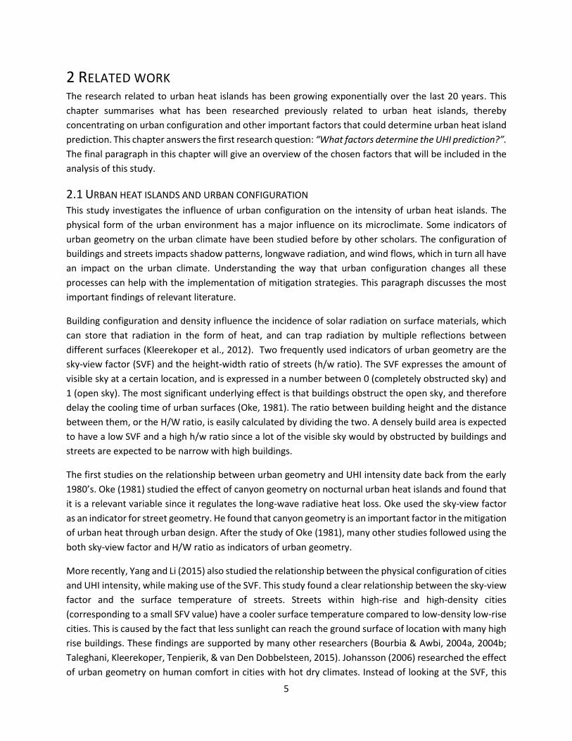
Moreover, similar dwelling or population density values can have completely different urban

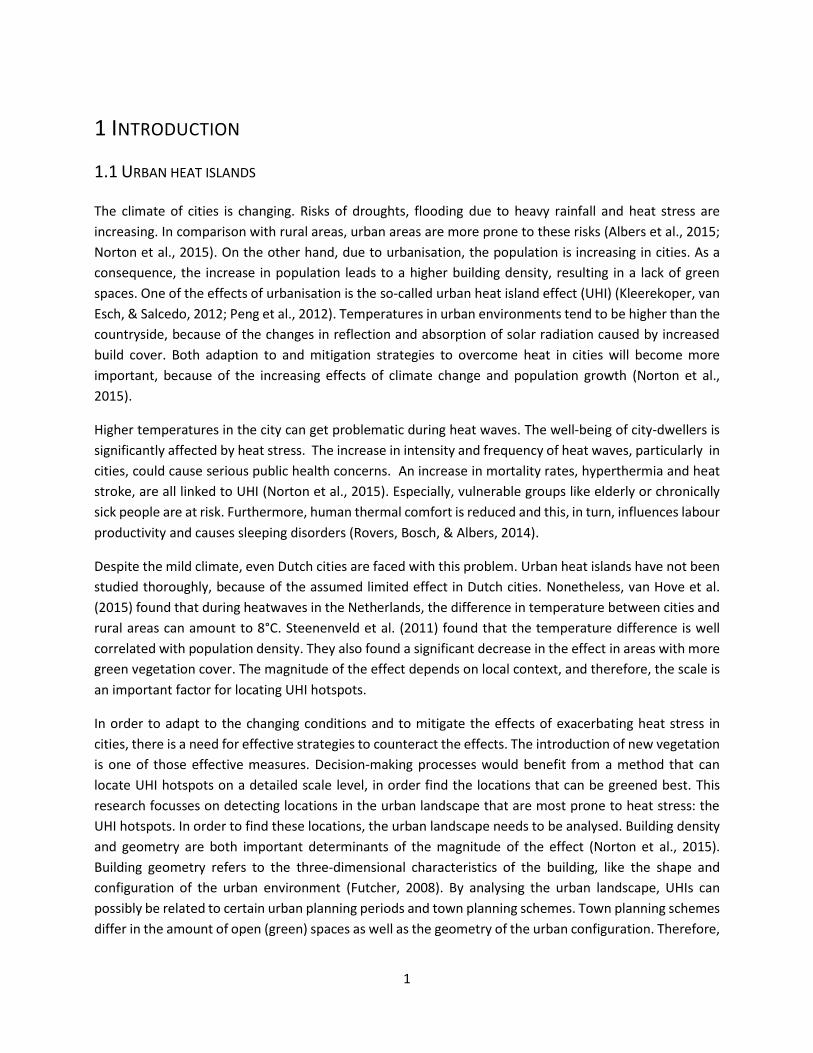
configurations. For example, Figure 1 shows that a density of 75 dwellings per hectare can be the result of

very different physical forms.

Figure 1 - 75 dwelling per hectare (Fernandez & Mozas, 2004)

Berghauser Pont and Haupt (2010) state the following: “The reasons that dwelling and population density

demonstrate a weak relation to built form are threefold: the occupancy rate of dwellings differs, the size

of dwellings differs and the amount of non-residential space is not taken into account when expressing

dwelling density” (p. 85). To conclude from this: both dwelling and population density are poor indicators

for building configuration and unfit for the purpose of this study. However, density remains an import

concept in daily planning practice and there is a need for clarification of the concept. In their book,

Berghauser Pont and Haupt (2010) investigate the potential for a combination of other types of density

measures to describe building configuration. By defining density as a multi-variable phenomenon, the

relation between density and building configuration can become clear. The next paragraph describes how

the spacematrix indicators can be used for this purpose and how the density measures can be calculated

using geo-data.

9

2.4 URBAN MATRIX INDICATORS The previous paragraphs described the present theoretical aspects of the influence of building

configuration on the extent of the UHI effect. However, the urban planning process would benefit from a

method that links UHI intensity to density variables. Berghauser Pont and Haupt have explored three

useful density variables that make the urban configuration measurable:

Floor Space Index (FSI) – gives an indication of the land use/build intensity by dividing the total

amount of floor space (F) within the defined area (x) by the base land area (A).

𝐹𝑆𝐼 = 𝐹𝑥

𝐴𝑥

The floor space index is a purely physical density indicator. It sums up all the floor space within an

area, independent of its use. This makes the FSI a great indicator for the purposes of this study,

since UHI intensity is not dependant on the use of buildings. Although the FSI makes a better

estimation of urban configuration than dwelling or population, FSI by itself is does not sufficient.

Areas with similar FSIs can still have completely different physical forms.

Gross Space Index (GSI) – describes the compactness of an area by determining the relationship

between non-built and built space. It is calculated by dividing the sum of the building footprint

area (B) within the defined area (x) by the base land area (A).

𝐺𝑆𝐼 = 𝐵𝑥

𝐴𝑥

The gross space index can be used to describe the distribution of open space and built mass. In

the Dutch planning system, it is used to regulate the maximum exploitation of an area. The GSI is

a better indicator of the spatial differences, but it needs to be supplemented by other indicators

since the indicator does not indicate the building height.

Open Space Ratio (OSR) – quantifies the spaciousness of an area by looking at the amount of floor

space in comparison to the unbuilt area. It indicates the pressure on the non-build space.

𝑂𝑅𝑆 = 1 − 𝐺𝑆𝐼𝑥

𝐹𝑆𝐼𝑥

The open space ratio indicates the relationship between open space and the built intensity of the

area. The OSR decreases when the amount of floor space within an area is increased, or when the

built up area increases. This tells us something about the spaciousness of the area, since a higher

OSR value results in a more open character.

The three indicators alone do not express urban configuration, but they can complement each other. By

combining these three variables the relationship between urban form and urban density can become clear.

Spaces with the same density do not necessarily have to have a similar urban configuration. However, the

urban

10

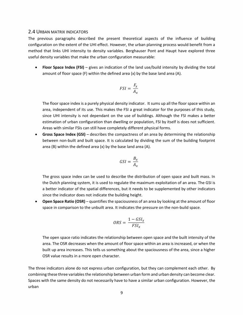
configuration may have an

influence on the extent of

UHIs. By making use of the

spacematrix indicators,

differences in urban

configuration can be included

in the analysis and related to

UHIs by making use of

temperature data. Berghauser

Pont and Haupt (2010)

illustrate this by making use of

the pile of blocks shown in

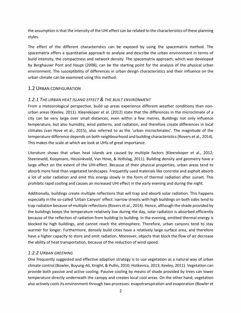
Figure 2 and the corresponding

table 1 . The three examples all

hold 4 blocks of the same size,

which illustrate the amount of

floor space, so in all the

examples the floor space is

four. The base land area, the

circle on the bottom, is

identical in all the examples,

also four. This causes the FSI to be 1 for all the examples. However, the footprint of the blocks is different

in the three examples (4, 2 and 1 respectively). This influences the GSI and OSR values. The GSI for example

2 is 0,5: half of the circle is covered with blocks. Consequently, the GSI of the third stack of blocks is equal

to 0,25. The OSR is 0 for the first example since the complete circle is covered. The OSR of the second and

third example equal 0,5 and 0,75. By expressing density with a combination of these indicators, the relation

to urban form can be made.

To calculate the three spacematrix indicators, three different measurable parameters are needed, namely:

the base land area, gross floor area and build up area.

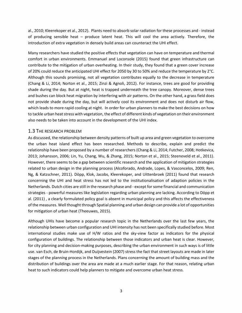
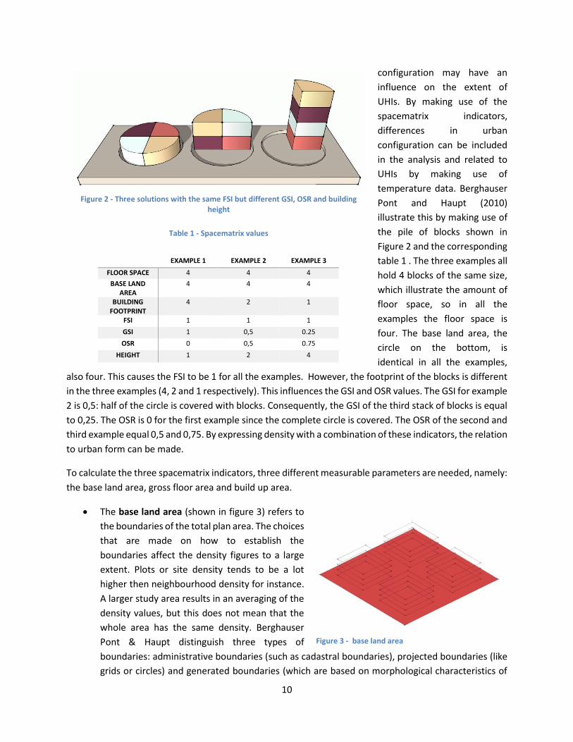
The base land area (shown in figure 3) refers to

the boundaries of the total plan area. The choices

that are made on how to establish the

boundaries affect the density figures to a large

extent. Plots or site density tends to be a lot

higher then neighbourhood density for instance.

A larger study area results in an averaging of the

density values, but this does not mean that the

whole area has the same density. Berghauser

Pont & Haupt distinguish three types of

boundaries: administrative boundaries (such as cadastral boundaries), projected boundaries (like

grids or circles) and generated boundaries (which are based on morphological characteristics of

Figure 2 - Three solutions with the same FSI but different GSI, OSR and building

height

Table 1 - Spacematrix values

EXAMPLE 1 EXAMPLE 2 EXAMPLE 3

FLOOR SPACE 4 4 4

BASE LAND AREA

4 4 4

BUILDING FOOTPRINT

4 2 1

FSI 1 1 1

GSI 1 0,5 0.25

OSR 0 0,5 0.75

HEIGHT 1 2 4

Figure 3 - base land area

11

the area). In this study, we focus on the neighbourhood level (an administrative boundary). When

we look at neighbourhoods (dutch: buurt) in the Netherlands, the amount of non-built space

increases when we zoom out from street scale to neighbourhood scale. Relatively more green

space, infrastructure and water are included at a larger scale, and therefore, these elements have

more influence on the density values. In this study, the definition of the Dutch central bureau of

statistics is used. The CBS (n.d.) states that “a neighbourhood is part of a municipality, that has

been homogeneously delimited based on historical or architectural characteristics”.

Homogeneously means that one type of use (residential, leisure, business or industry) is

predominantly present in the neighbourhood, but also mixed use is possible. In the Netherlands,

municipalities are divided into districts (dutch: wijken), districts are divided into neighbourhoods.

This makes neighbourhoods the lowest regional level.

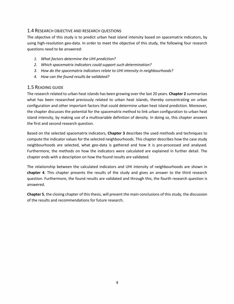
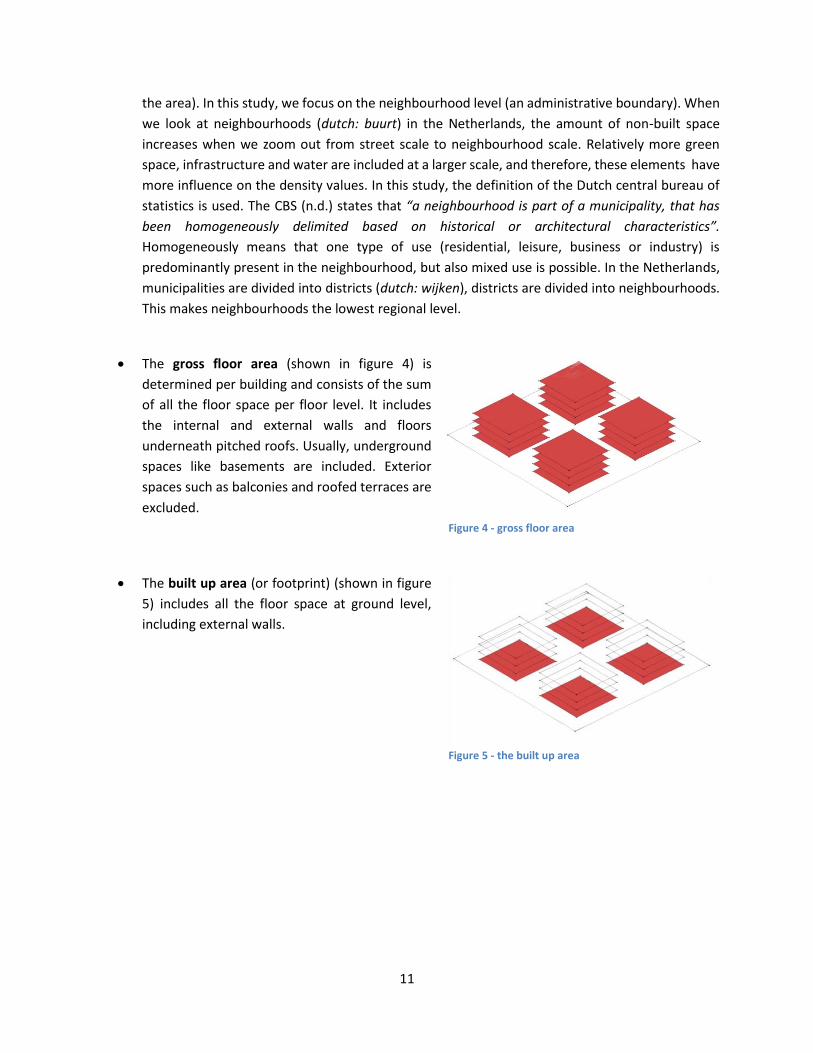
The gross floor area (shown in figure 4) is

determined per building and consists of the sum

of all the floor space per floor level. It includes

the internal and external walls and floors

underneath pitched roofs. Usually, underground

spaces like basements are included. Exterior

spaces such as balconies and roofed terraces are

excluded.

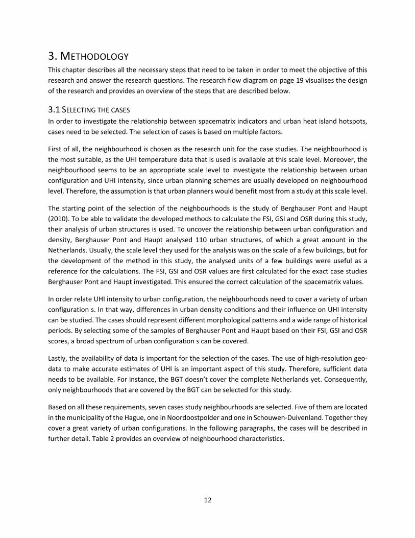
The built up area (or footprint) (shown in figure

5) includes all the floor space at ground level,

including external walls.

Figure 4 - gross floor area

Figure 5 - the built up area

12

3. METHODOLOGY This chapter describes all the necessary steps that need to be taken in order to meet the objective of this

research and answer the research questions. The research flow diagram on page 19 visualises the design

of the research and provides an overview of the steps that are described below.

3.1 SELECTING THE CASES In order to investigate the relationship between spacematrix indicators and urban heat island hotspots,

cases need to be selected. The selection of cases is based on multiple factors.

First of all, the neighbourhood is chosen as the research unit for the case studies. The neighbourhood is

the most suitable, as the UHI temperature data that is used is available at this scale level. Moreover, the

neighbourhood seems to be an appropriate scale level to investigate the relationship between urban

configuration and UHI intensity, since urban planning schemes are usually developed on neighbourhood

level. Therefore, the assumption is that urban planners would benefit most from a study at this scale level.

The starting point of the selection of the neighbourhoods is the study of Berghauser Pont and Haupt

(2010). To be able to validate the developed methods to calculate the FSI, GSI and OSR during this study,

their analysis of urban structures is used. To uncover the relationship between urban configuration and

density, Berghauser Pont and Haupt analysed 110 urban structures, of which a great amount in the

Netherlands. Usually, the scale level they used for the analysis was on the scale of a few buildings, but for

the development of the method in this study, the analysed units of a few buildings were useful as a

reference for the calculations. The FSI, GSI and OSR values are first calculated for the exact case studies

Berghauser Pont and Haupt investigated. This ensured the correct calculation of the spacematrix values.

In order relate UHI intensity to urban configuration, the neighbourhoods need to cover a variety of urban

configuration s. In that way, differences in urban density conditions and their influence on UHI intensity

can be studied. The cases should represent different morphological patterns and a wide range of historical

periods. By selecting some of the samples of Berghauser Pont and Haupt based on their FSI, GSI and OSR

scores, a broad spectrum of urban configuration s can be covered.

Lastly, the availability of data is important for the selection of the cases. The use of high-resolution geo-

data to make accurate estimates of UHI is an important aspect of this study. Therefore, sufficient data

needs to be available. For instance, the BGT doesn’t cover the complete Netherlands yet. Consequently,

only neighbourhoods that are covered by the BGT can be selected for this study.

Based on all these requirements, seven cases study neighbourhoods are selected. Five of them are located

in the municipality of the Hague, one in Noordoostpolder and one in Schouwen-Duivenland. Together they

cover a great variety of urban configurations. In the following paragraphs, the cases will be described in

further detail. Table 2 provides an overview of neighbourhood characteristics.

13

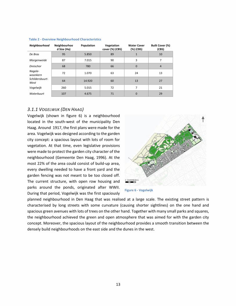
Table 2 - Overview Neighbourhood Characteristics

3.1.1 VOGELWIJK (DEN HAAG) Vogelwijk (shown in figure 6) is a neighbourhood

located in the south-west of the municipality Den

Haag. Around 1917, the first plans were made for the

area. Vogelwijk was designed according to the garden

city concept: a spacious layout with lots of room for

vegetation. At that time, even legislative provisions

were made to protect the garden city character of the

neighbourhood (Gemeente Den Haag, 1996). At the

most 22% of the area could consist of build-up area,

every dwelling needed to have a front yard and the

garden fencing was not meant to be too closed off.

The current structure, with open row housing and

parks around the ponds, originated after WWII.

During that period, Vogelwijk was the first spaciously

planned neighbourhood in Den Haag that was realised at a large scale. The existing street pattern is

characterised by long streets with some curvature (causing shorter sightlines) on the one hand and

spacious green avenues with lots of trees on the other hand. Together with many small parks and squares,

the neighbourhood achieved the green and open atmosphere that was aimed for with the garden city

concept. Moreover, the spacious layout of the neighbourhood provides a smooth transition between the

densely build neighbourhoods on the east side and the dunes in the west.

Neighbourhood Neighbourhood Size (Ha)

Population Vegetation cover (%) (CBS)

Water Cover (%) (CBS)

Built Cover (%) (CBS)

De Bras 95 5.850 89 1 10

Morgenweide 87 7.015 90 3 7

Dreischor 68 780 66 0 4

Nagele-woonkern

72 1.070 63 24 13

Schildersbuurt-West

64 14.920 60 13 27

Vogelwijk 260 5.015 72 7 21

Waterbuurt 107 4.675 71 0 29

Figure 6 - Vogelwijk

14

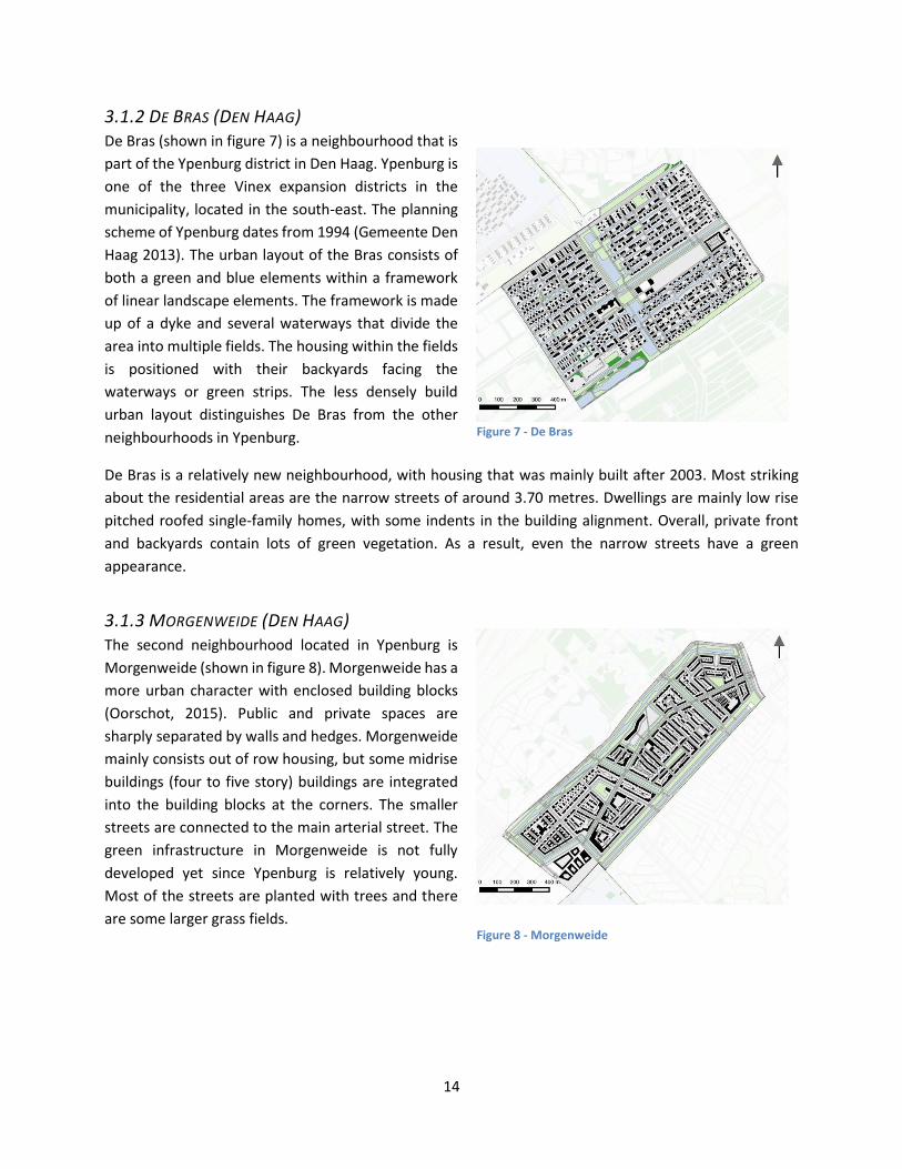
3.1.2 DE BRAS (DEN HAAG) De Bras (shown in figure 7) is a neighbourhood that is

part of the Ypenburg district in Den Haag. Ypenburg is

one of the three Vinex expansion districts in the

municipality, located in the south-east. The planning

scheme of Ypenburg dates from 1994 (Gemeente Den

Haag 2013). The urban layout of the Bras consists of

both a green and blue elements within a framework

of linear landscape elements. The framework is made

up of a dyke and several waterways that divide the

area into multiple fields. The housing within the fields

is positioned with their backyards facing the

waterways or green strips. The less densely build

urban layout distinguishes De Bras from the other

neighbourhoods in Ypenburg.

De Bras is a relatively new neighbourhood, with housing that was mainly built after 2003. Most striking

about the residential areas are the narrow streets of around 3.70 metres. Dwellings are mainly low rise

pitched roofed single-family homes, with some indents in the building alignment. Overall, private front

and backyards contain lots of green vegetation. As a result, even the narrow streets have a green

appearance.

3.1.3 MORGENWEIDE (DEN HAAG) The second neighbourhood located in Ypenburg is

Morgenweide (shown in figure 8). Morgenweide has a

more urban character with enclosed building blocks

(Oorschot, 2015). Public and private spaces are

sharply separated by walls and hedges. Morgenweide

mainly consists out of row housing, but some midrise

buildings (four to five story) buildings are integrated

into the building blocks at the corners. The smaller

streets are connected to the main arterial street. The

green infrastructure in Morgenweide is not fully

developed yet since Ypenburg is relatively young.

Most of the streets are planted with trees and there

are some larger grass fields.

Figure 7 - De Bras

Figure 8 - Morgenweide

15

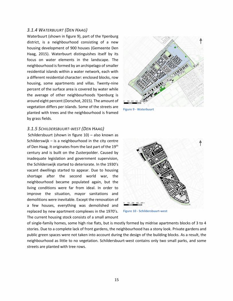
3.1.4 WATERBUURT (DEN HAAG) Waterbuurt (shown in figure 9), part of the Ypenburg

district, is a neighbourhood consisting of a new

housing development of 900 houses (Gemeente Den

Haag, 2015). Waterbuurt distinguishes itself by its

focus on water elements in the landscape. The

neighbourhood is formed by an archipelago of smaller

residential islands within a water network, each with

a different residential character: enclosed blocks, row

housing, some apartments and villas. Twenty-nine

percent of the surface area is covered by water while

the average of other neighbourhoods Ypenburg is

around eight percent (Oorschot, 2015). The amount of

vegetation differs per islands. Some of the streets are

planted with trees and the neighbourhood is framed

by grass fields.

3.1.5 SCHILDERSBUURT-WEST (DEN HAAG) Schildersbuurt (shown in figure 10) – also known as

Schilderswijk – is a neighbourhood in the city centre

of Den Haag. It originates from the last part of the 19th

century and is built on the Zusterpolder. Caused by

inadequate legislation and government supervision,

the Schilderswijk started to deteriorate. In the 1930’s

vacant dwellings started to appear. Due to housing

shortage after the second world war, the

neighbourhood became populated again, but the

living conditions were far from ideal. In order to

improve the situation, mayor sanitations and

demolitions were inevitable. Except the renovation of

a few houses, everything was demolished and

replaced by new apartment complexes in the 1970’s.

The current housing stock consists of a small amount

of single-family homes, some high rise flats, but is mostly formed by midrise apartments blocks of 3 to 4

stories. Due to a complete lack of front gardens, the neighbourhood has a stony look. Private gardens and

public green spaces were not taken into account during the design of the building blocks. As a result, the

neighbourhood as little to no vegetation. Schildersbuurt-west contains only two small parks, and some

streets are planted with tree rows.

Figure 9 - Waterbuurt

Figure 10 - Schildersbuurt-west

16

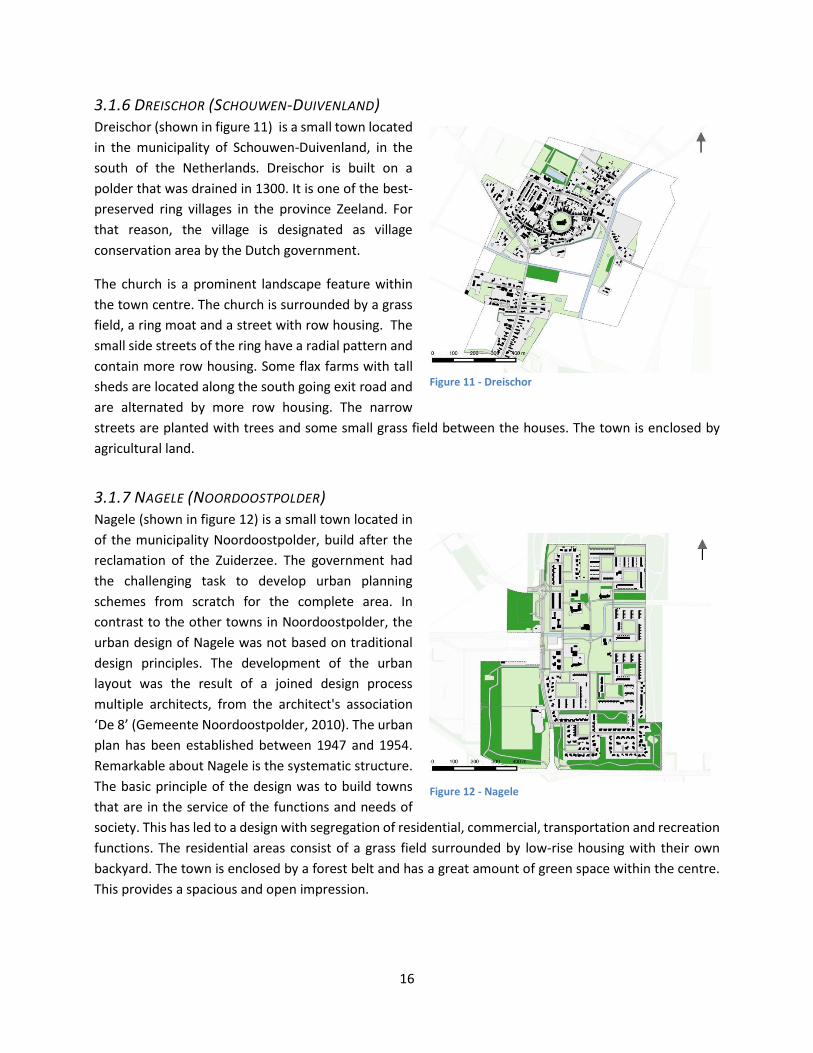
3.1.6 DREISCHOR (SCHOUWEN-DUIVENLAND) Dreischor (shown in figure 11) is a small town located

in the municipality of Schouwen-Duivenland, in the

south of the Netherlands. Dreischor is built on a

polder that was drained in 1300. It is one of the best-

preserved ring villages in the province Zeeland. For

that reason, the village is designated as village

conservation area by the Dutch government.

The church is a prominent landscape feature within

the town centre. The church is surrounded by a grass

field, a ring moat and a street with row housing. The

small side streets of the ring have a radial pattern and

contain more row housing. Some flax farms with tall

sheds are located along the south going exit road and

are alternated by more row housing. The narrow

streets are planted with trees and some small grass field between the houses. The town is enclosed by

agricultural land.

3.1.7 NAGELE (NOORDOOSTPOLDER) Nagele (shown in figure 12) is a small town located in

of the municipality Noordoostpolder, build after the

reclamation of the Zuiderzee. The government had

the challenging task to develop urban planning

schemes from scratch for the complete area. In

contrast to the other towns in Noordoostpolder, the

urban design of Nagele was not based on traditional

design principles. The development of the urban

layout was the result of a joined design process

multiple architects, from the architect's association

‘De 8’ (Gemeente Noordoostpolder, 2010). The urban

plan has been established between 1947 and 1954.

Remarkable about Nagele is the systematic structure.

The basic principle of the design was to build towns

that are in the service of the functions and needs of

society. This has led to a design with segregation of residential, commercial, transportation and recreation

functions. The residential areas consist of a grass field surrounded by low-rise housing with their own

backyard. The town is enclosed by a forest belt and has a great amount of green space within the centre.

This provides a spacious and open impression.

Figure 11 - Dreischor

Figure 12 - Nagele

17

3.2 DATA SELECTION AND PREPOSSESSING

For the purposes of this study, several geodata sources are used. The following datasets are used in this

study:

CBS neighbourhoods: This study analyses the relationship between urban configuration and

Urban Heat Island intensity on a neighbourhood scale. The Dutch central bureau of statistics (CBS)

provides the CBS Neighbourhood Map (2014) that includes the digital geometry of the boundaries

of the neighbourhoods in the Netherlands. The dataset also includes census data.

BGT: The main data source for this research should have been the BGT. The BGT is a high-

resolution digital map of the whole Netherlands that contains all physical objects related to

buildings, (rail)roads, water and vegetation. The map is not available yet for the whole Netherlands

and is scheduled to be finished in 2020. The BGT can be very useful for the purposes of this study.

The detailed map can be used to analyse the building density, urban configuration and the

presence of vegetation. However, working with the BGT dataset resulted in some difficulties. The

BGT, which is available in a GML-data format, couldn’t be loaded in ArcMap 10.3. Moreover, the

dataset is large and therefore unhandy to work with. A lot of information in the BGT is redundant

for this study, because only the buildings and vegetation are of interest. Therefore, the BGT data

needs to be supplemented by a combination of BAG data and height data from AHN2. However,

for the vegetation indicators, the vegetation layers of the BGT are used.

BAG: The collection of BGT data proved to be very challenging, and the BAG dataset provides the

most complete dataset concerning information about buildings. This led to the choice of using

BAG data to perform the calculations of the FSI, GSI and OSR values, instead of the BGT. The BAG

can be divided into the registration of addresses and buildings. For this study, the buildings dataset

is used. This dataset holds information about all buildings, residence properties, plots and

registered berths in the Netherlands.

AHN2: In order to calculate the spacematrix indicators, height information from the buildings is

also necessary. Therefore, the AHN2 dataset is also used in this study. The AHN is a height model

of the Netherlands that is produced using laser altimetry. The AHN2 0.5-metre filled ground level

raster is used in this study. All the non-ground level objects (like trees, buildings, bridges, and other

objects) have been filtered out of this dataset. The no-data cells resulting from this filtering, are

not filled. Because the buildings are of interest in this study, the raw AHN2 0.5-meter grid is also

used. In contrast to the filled dataset, the raw grid still contains height data from non-ground

objects like buildings and trees. By using both the raw and the filled dataset, building heights can

be calculated.

Tree Canopy Polygons: Besides the vegetation layers of the BGT, additional data from the dataset

the ‘Tree Canopy Polygons’ dataset from Meijer, Rip, Benthem, and Clement (2015) is also

included in the calculation of the vegetation indicators. This is a national coverage dataset with

information on all tree crowns in the Netherlands.

Temperature data: To link the urban density factors to UHI temperature, a UHI intensity dataset

on neighbourhood level is used. More information about the used temperature data can be found

in paragraph 3.5.

18

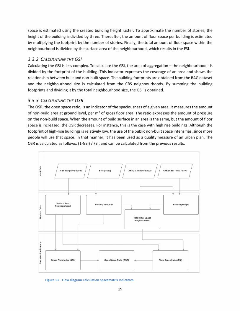
3.3 CALCULATING SPACEMATRIX INDICATORS This paragraph describes the necessary steps for calculating the spacematrix indicators: the Floor Space

Index, the Gross Space index and the Open Space Ratio. The flow diagram on page 19 visualises the steps

that were followed.

3.3.1 CALCULATING THE FSI In order to calculate the Floor Space index (FSI) for a neighbourhood, several datasets are necessary. The

FSI indicates the relationship between the amount of floor space and the surface area of the

neighbourhood, which gives an indication of the building intensity. In order to calculate this, two variables

are needed: the amount of floor space, and the surface area of the neighbourhood. The latter can be

obtained quite easily from the ‘CBS Neighbourhoods dataset, by looking at the shape area of the polygon.

However, making an accurate estimation of total the floor space within the neighbourhood is less

straightforward. The following paragraph explains in further detail how the FSI is calculated.

The amount of floor space within a neighbourhood is calculated based on two datasets: the BAG and AHN2

dataset. Within the BAG, the amount of floor space inside a building is indicated per property, but only the

maximum and the minimum surface area size are given. When the number of properties within a building

is 1, for instance in the case of a single family home, the surface area is easily translated into the amount

of floor space. This is also the case with two properties in one building. However, when the number of

properties within a building is larger than two, not all floor spaces are known. It cannot be assumed that

every property within a building has the same size. Therefore, the total amount of floor space has to be

calculated by other means.

A way to get around this problem is to calculate the footprint and the height of a building. The amount of

floor space can then be estimated by dividing the height of the building by the average story height (which

is around 3 metres) and multiplying that by the footprint of the building. The footprint is obtained by

making use of the BAG. However, the height of the building is not registered in this dataset.

The height of buildings can be obtained from the AHN2 dataset. The final product of the AHN2 is a digital

terrain model of the Netherlands, not a surface model. This means that all buildings heights are filtered

out from the model. In order to calculate building height, the raw AHN2 data is necessary which still

contains all building heights. By subtracting the filled surface grid from the raw AHN2 data at the location

of buildings, the building height can be obtained.

However, the filled AHN2 surface grid itself contains gaps on the locations of buildings, because they are

filtered out. In order to make an estimation of the surface height underneath buildings, focal statistics are

used to interpolate the height values. The minimum height value of the pixels within a radius of 20 cells

(10 metres respectively) surrounding the building is assigned to all null values below the buildings.

Subsequently, the mean height per building is calculated from the raw AHN2 raster using zonal statistics.

By subtracting the two created grids, a new raster with all building heights is created.

At this stage, all needed variables are present for the calculation of the FSI. The amount of floor space for

all buildings containing one or two properties is calculated using the minimum and maximum floor space

attributes indicated in the BAG. For every building with more than two properties, the amount of floor

19

space is estimated using the created building height raster. To approximate the number of stories, the

height of the building is divided by three. Thereafter, the amount of floor space per building is estimated

by multiplying the footprint by the number of stories. Finally, the total amount of floor space within the

neighbourhood is divided by the surface area of the neighbourhood, which results in the FSI.

3.3.2 CALCULATING THE GSI Calculating the GSI is less complex. To calculate the GSI, the area of aggregation – the neighbourhood - is

divided by the footprint of the building. This indicator expresses the coverage of an area and shows the

relationship between built and non-built space. The building footprints are obtained from the BAG dataset

and the neighbourhood size is calculated from the CBS neighbourhoods. By summing the building

footprints and dividing it by the total neighbourhood size, the GSI is obtained.

3.3.3 CALCULATING THE OSR The OSR, the open space ratio, is an indicator of the spaciousness of a given area. It measures the amount

of non-build area at ground level, per m2 of gross floor area. The ratio expresses the amount of pressure

on the non-build space. When the amount of build surface in an area is the same, but the amount of floor

space is increased, the OSR decreases. For instance, this is the case with high rise buildings. Although the

footprint of high-rise buildings is relatively low, the use of the public non-built space intensifies, since more

people will use that space. In that manner, it has been used as a quality measure of an urban plan. The

OSR is calculated as follows: (1-GSI) / FSI, and can be calculated from the previous results.

Figure 13 – Flow diagram Calculation Spacematrix Indicators

20

3.4 CALCULATING OTHER INDICATORS

3.4.1 SKY-VIEW FACTOR In order to relate the impact of urban geometry on UHI intensity, the sky view factor (SVF) is a frequently

used as an indicator of the temperature differences between the surfaces in urban environments (Yang &

Li, 2015). Initially, the SVF was computed by using a fish- eye camera. By making a photograph looking

upward from ground level, the percentage of obstructed sky can be determined from the photo. However,

the SVF can also be estimated using GIS and a digital elevation model. SAGA GIS offers a terrain analysis

tool that analyses a DEM and calculates the SVF for every location, based on the cell height variation.

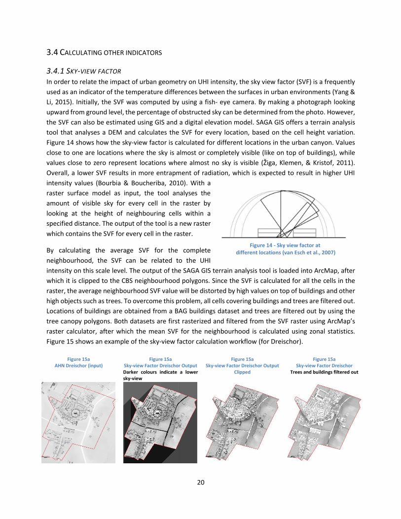
Figure 14 shows how the sky-view factor is calculated for different locations in the urban canyon. Values

close to one are locations where the sky is almost or completely visible (like on top of buildings), while

values close to zero represent locations where almost no sky is visible (Žiga, Klemen, & Kristof, 2011).

Overall, a lower SVF results in more entrapment of radiation, which is expected to result in higher UHI

intensity values (Bourbia & Boucheriba, 2010). With a

raster surface model as input, the tool analyses the

amount of visible sky for every cell in the raster by

looking at the height of neighbouring cells within a

specified distance. The output of the tool is a new raster

which contains the SVF for every cell in the raster.

By calculating the average SVF for the complete

neighbourhood, the SVF can be related to the UHI

intensity on this scale level. The output of the SAGA GIS terrain analysis tool is loaded into ArcMap, after

which it is clipped to the CBS neighbourhood polygons. Since the SVF is calculated for all the cells in the

raster, the average neighbourhood SVF value will be distorted by high values on top of buildings and other

high objects such as trees. To overcome this problem, all cells covering buildings and trees are filtered out.

Locations of buildings are obtained from a BAG buildings dataset and trees are filtered out by using the

tree canopy polygons. Both datasets are first rasterized and filtered from the SVF raster using ArcMap’s

raster calculator, after which the mean SVF for the neighbourhood is calculated using zonal statistics.

Figure 15 shows an example of the sky-view factor calculation workflow (for Dreischor).

Figure 14 - Sky view factor at

different locations (van Esch et al., 2007)

Figure 15a AHN Dreischor (input)

Figure 15a Sky-view Factor Dreischor Output Darker colours indicate a lower sky-view

Figure 15a Sky-view Factor Dreischor Output

Clipped

Figure 15a Sky-view Factor Dreischor

Trees and buildings filtered out

21

3.4.2 TREE AND VEGETATION DENSITY The extent of UHI’s is often related to the amount of vegetation within an area. The presence of vegetation

is complementary to urban configuration. Trees - particularly large trees - shade and cool the surface

temperature by preventing solar radiation from reaching the surface, and cooling the environment

through evapotranspiration (Rovers et al., 2014).

The availability of the Tree Canopy Polygon dataset makes it possible to examine the cumulative effect of

individual trees within the neighbourhood on the UHI intensity. The dataset contains both public and

private trees. The surface area that is covered by trees can be calculated by making use this dataset. The

method to calculate the tree density is straightforward: by summing the surface area covered by trees and

dividing it by the surface area of the neighbourhood, the percentage of ground covered by trees can be

calculated.

In addition to the tree density, the vegetation density is also calculated. The BGT dataset is used to

calculate the fraction of surface area of the neighbourhood that is covered by vegetation. The vegetation

density is derived by applying the same method: the surface area covered by vegetation was summed, and

divided by size of the neighbourhood.

3.5 INCLUDING TEMPERATURE DATA

3.5.1 THE DATA In order to link the calculated spacematrix and vegetation indicators, temperature data is necessary. In

this study, the temperature data is coming from a high-resolution weather forecasting model, that

provides estimations of UHI intensity at neighbourhood scale spatial resolution for the complete

Netherlands. The model was developed by Holtslag, Ronda, Steeneveld, Heusinkveld, and Harst (2013),

and it is based on multiple data sources. Height data is included, which is a traditional input for weather

models. Furthermore, data from the central bureau of statistics (CBS) for information about population

density, and aerial photographs to make estimations of the green fraction of a neighbourhood, and land-

use data from the TOP10NL dataset from the Dutch Cadastre. The forecasting model is validated by the

use of observational data, gathered from observation networks (30 meteorological weather stations),

measurement campaigns, and crowd-sourced data.

The reason that this estimated UHI intensity data is used, instead of observational data, is because

observational data on neighbourhood level is rare. Moreover, in order to make reliable comparisons

between the spacematrix values of different neighbourhoods, the UHI intensity data should also be

comparable. To meet these requirements, all the temperature data should have been gathered on the

same day, under similar circumstances. This kind of data is not available for the selected cases, and the

estimated UHI intensity data used in this study is an adequate substitute for observational data.

3.5.2 PREPOSSESSING UHI DATA The temperature dataset contains information about the estimated Urban Heat Island intensity per

neighbourhood for the Netherlands. This information is stored in an excel table. To be able to analyse the

data within ArcMap, the data needs to be linked to the CBS neighbourhoods dataset. The table is first

22

Neighbourhood Neighbourhoo

d Size (Ha) Population

UHI Intensity (⁰C)

Vegetation cover (CBS)

Water Cover (CBS)

Built Cover (CBS)

Wageningen Hoog (Wageningen)

158 1200 1,8 97 0 3

Cool (Rotterdam) 61 4320 5,17 47 1 51

Geuzenveld (Amsterdam) 142 14360 4,74 71 7 22

Douve Weien (Heerlen) 79 3730 3,63 84 0 16

Colijnsplaat (Noord-Beveland)

158 1200 1,8 97 0 3

Vijfhuizen Stellinghof (Haarlemmermeer)

50 1850 3,61 78 11 11

Indische Buurt West (Amsterdam)

49 12685 6,52 46 3 51

Barger-Erfscheidenveen (Emmen)

44 115 1,23 94 2 3

imported into a geodatabase, after which it is joined to the neighbourhood polygons, based on both

municipality and neighbourhood name.

3.5.3 REGRESSION After the calculation of all the indicator values for the neighbourhoods, the relationship between the

indicators and the UHI intensity is investigated. It would be interesting to find out if it is possible to predict

the UHI intensity based on the spacematrix indicator values of a neighbourhood. This is possible by making

use of simple linear regression analysis. The hypothesis is that there is a linear relationship between the

indicator values of a neighbourhood and the expected UHI intensity. By means of scatterplots, the found

indicator values are plotted against the UHI intensity values. In order to test the hypothesis, the estimation

of the relationship is done by fitting a linear trend line (the least squares estimator) through the data

points. The dependent variable (the UHI intensity) is estimated through one of the independent variables

(the indicators). The correlation between the UHI intensity and the indicators is examined by making use

of the R2 (the coefficient of determination). The R2 describes how well the trend line fits through the data,

thereby providing information about to what extent the independent variable explains the variation in the

dependent variable. The R2 ranges from 0 to 1. An R2 of 0 indicates that the line does not fit the data, and

a value of 1 indicates that the line fits the data perfectly.

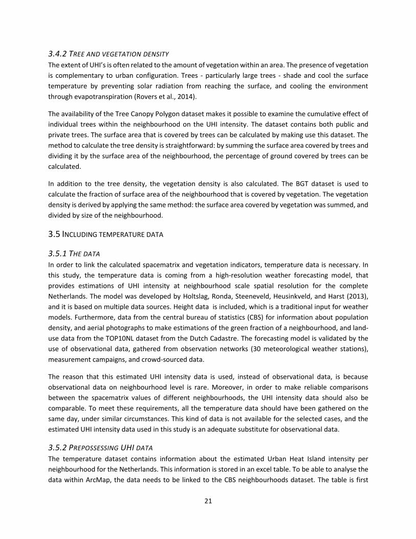
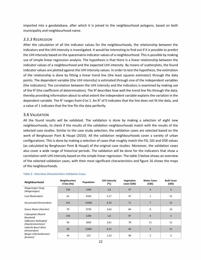
3.6 VALIDATION All the found results will be validated. The validation is done by making a selection of eight new

neighbourhoods, to check if the results of the validation neighbourhoods match with the results of the

selected case studies. Similar to the case study selection, the validation cases are selected based on the

work of Berghauser Pont & Haupt (2010). All the validation neighbourhoods cover a variety of urban

configurations. This is done by making a selection of cases that roughly match the FSI, GSI and OSR values

(as calculated by Berghauser Pont & Haupt) of the original case studies. Moreover, the validation cases

also cover a wide range of historical periods. The validation will be done for the indicators that show a

correlation with UHI intensity based on the simple linear regression. The table 3 below shows an overview

of the selected validation cases, with their most significant characteristics and figure 16 shows the maps

of the neighbourhoods.

Table 3 - Overview Characteristics Validation Cases

23

Figure 16a - Wageningen Hoog Figure 16b - Cool

Figure 16c - Geuzenveld Figure 16d - Douve Weien

24

Figure 16e - Colijnsplaat Figure 16f - Vijfhuizen Stellinghof

Figure 16g - Indische Buurt West Figure 16h - Barger-Erfscheidenveen

25

4 RESULTS AND VALIDATION This chapter presents the most important found results of the relation between urban heat island intensity

and spacematrix indicators and answers the third research question: “How do the spacematrix indicators

relate to UHI intensity in neighbourhoods?”. First, the results of the spacematrix indicators (FSI, GSI and

OSR) are presented in paragraph 4.1. The results of the other indicators are explained in paragraph 4.2,

after which the results are validated in paragraph 4.3.

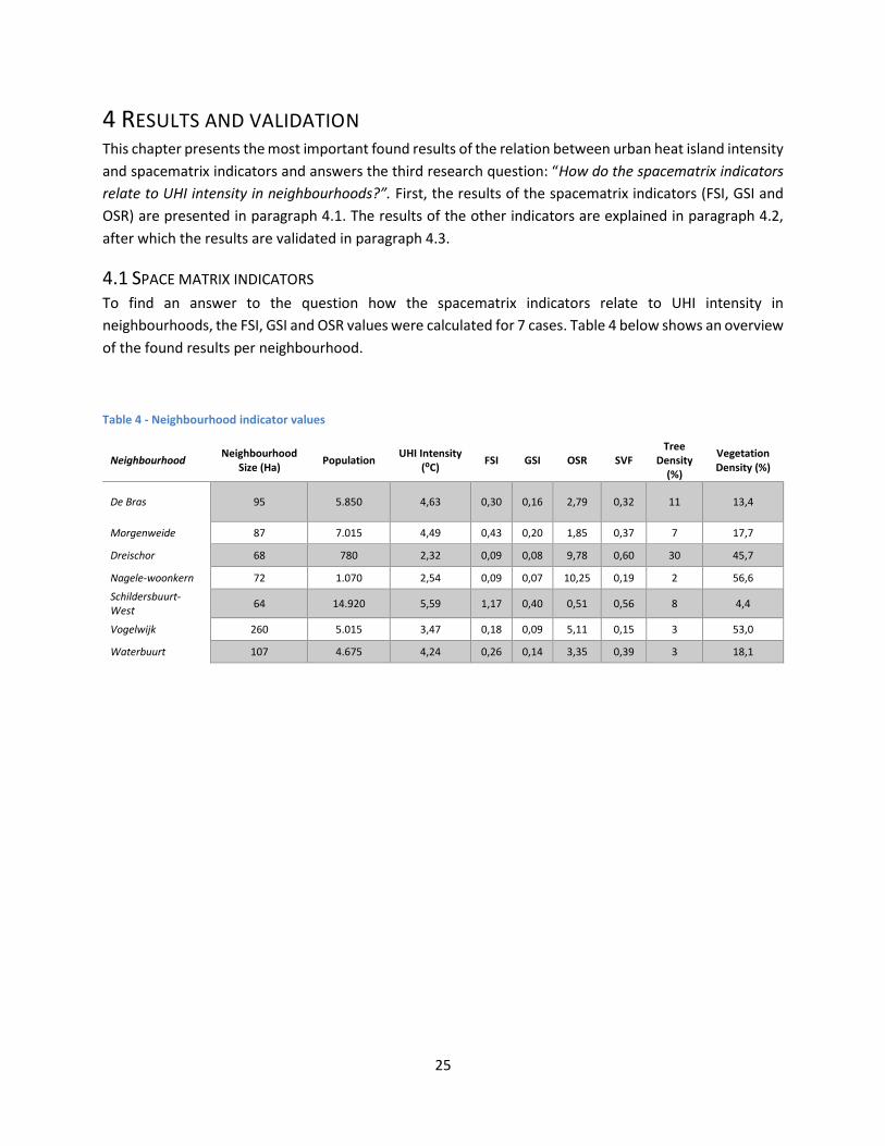
4.1 SPACE MATRIX INDICATORS To find an answer to the question how the spacematrix indicators relate to UHI intensity in

neighbourhoods, the FSI, GSI and OSR values were calculated for 7 cases. Table 4 below shows an overview

of the found results per neighbourhood.

Table 4 - Neighbourhood indicator values

Neighbourhood Neighbourhood

Size (Ha) Population

UHI Intensity (⁰C)

FSI GSI OSR SVF Tree

Density (%)

Vegetation Density (%)

De Bras 95 5.850 4,63 0,30 0,16 2,79 0,32 11 13,4

Morgenweide 87 7.015 4,49 0,43 0,20 1,85 0,37 7 17,7

Dreischor 68 780 2,32 0,09 0,08 9,78 0,60 30 45,7

Nagele-woonkern 72 1.070 2,54 0,09 0,07 10,25 0,19 2 56,6

Schildersbuurt-West

64 14.920 5,59 1,17 0,40 0,51 0,56 8 4,4

Vogelwijk 260 5.015 3,47 0,18 0,09 5,11 0,15 3 53,0

Waterbuurt 107 4.675 4,24 0,26 0,14 3,35 0,39 3 18,1

26

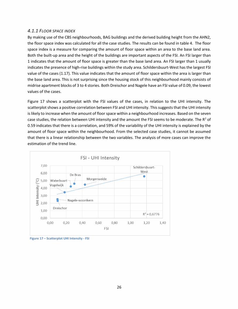
4.1.1 FLOOR SPACE INDEX By making use of the CBS neighbourhoods, BAG buildings and the derived building height from the AHN2,

the floor space index was calculated for all the case studies. The results can be found in table 4. The floor

space index is a measure for comparing the amount of floor space within an area to the base land area.

Both the built-up area and the height of the buildings are important aspects of the FSI. An FSI larger than

1 indicates that the amount of floor space is greater than the base land area. An FSI larger than 1 usually

indicates the presence of high-rise buildings within the study area. Schildersbuurt-West has the largest FSI

value of the cases (1.17). This value indicates that the amount of floor space within the area is larger than

the base land area. This is not surprising since the housing stock of this neighbourhood mainly consists of

midrise apartment blocks of 3 to 4 stories. Both Dreischor and Nagele have an FSI value of 0.09, the lowest

values of the cases.

Figure 17 shows a scatterplot with the FSI values of the cases, in relation to the UHI intensity. The

scatterplot shows a positive correlation between FSI and UHI intensity. This suggests that the UHI intensity

is likely to increase when the amount of floor space within a neighbourhood increases. Based on the seven

case studies, the relation between UHI intensity and the amount the FSI seems to be moderate. The R2 of

0.59 indicates that there is a correlation, and 59% of the variability of the UHI intensity is explained by the

amount of floor space within the neighbourhood. From the selected case studies, it cannot be assumed

that there is a linear relationship between the two variables. The analysis of more cases can improve the

estimation of the trend line.

Figure 17 – Scatterplot UHI Intensity - FSI

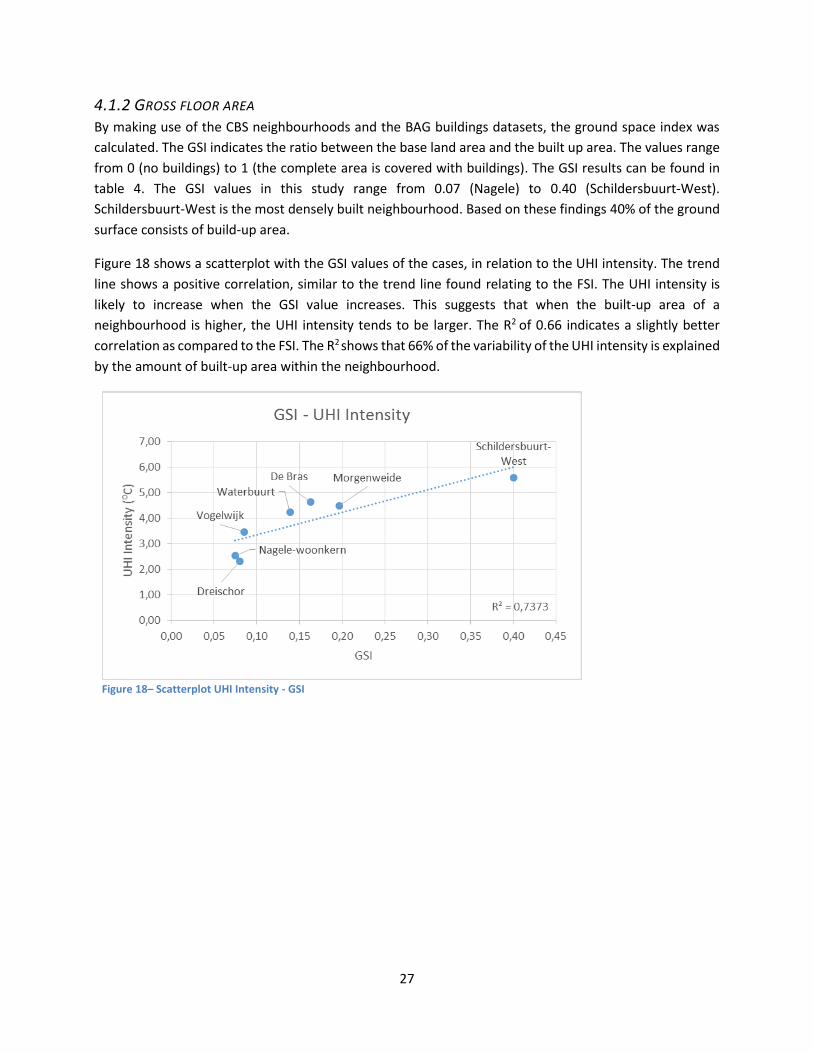
27

4.1.2 GROSS FLOOR AREA By making use of the CBS neighbourhoods and the BAG buildings datasets, the ground space index was

calculated. The GSI indicates the ratio between the base land area and the built up area. The values range

from 0 (no buildings) to 1 (the complete area is covered with buildings). The GSI results can be found in

table 4. The GSI values in this study range from 0.07 (Nagele) to 0.40 (Schildersbuurt-West).

Schildersbuurt-West is the most densely built neighbourhood. Based on these findings 40% of the ground

surface consists of build-up area.

Figure 18 shows a scatterplot with the GSI values of the cases, in relation to the UHI intensity. The trend

line shows a positive correlation, similar to the trend line found relating to the FSI. The UHI intensity is

likely to increase when the GSI value increases. This suggests that when the built-up area of a

neighbourhood is higher, the UHI intensity tends to be larger. The R2 of 0.66 indicates a slightly better

correlation as compared to the FSI. The R2 shows that 66% of the variability of the UHI intensity is explained

by the amount of built-up area within the neighbourhood.

Figure 18– Scatterplot UHI Intensity - GSI

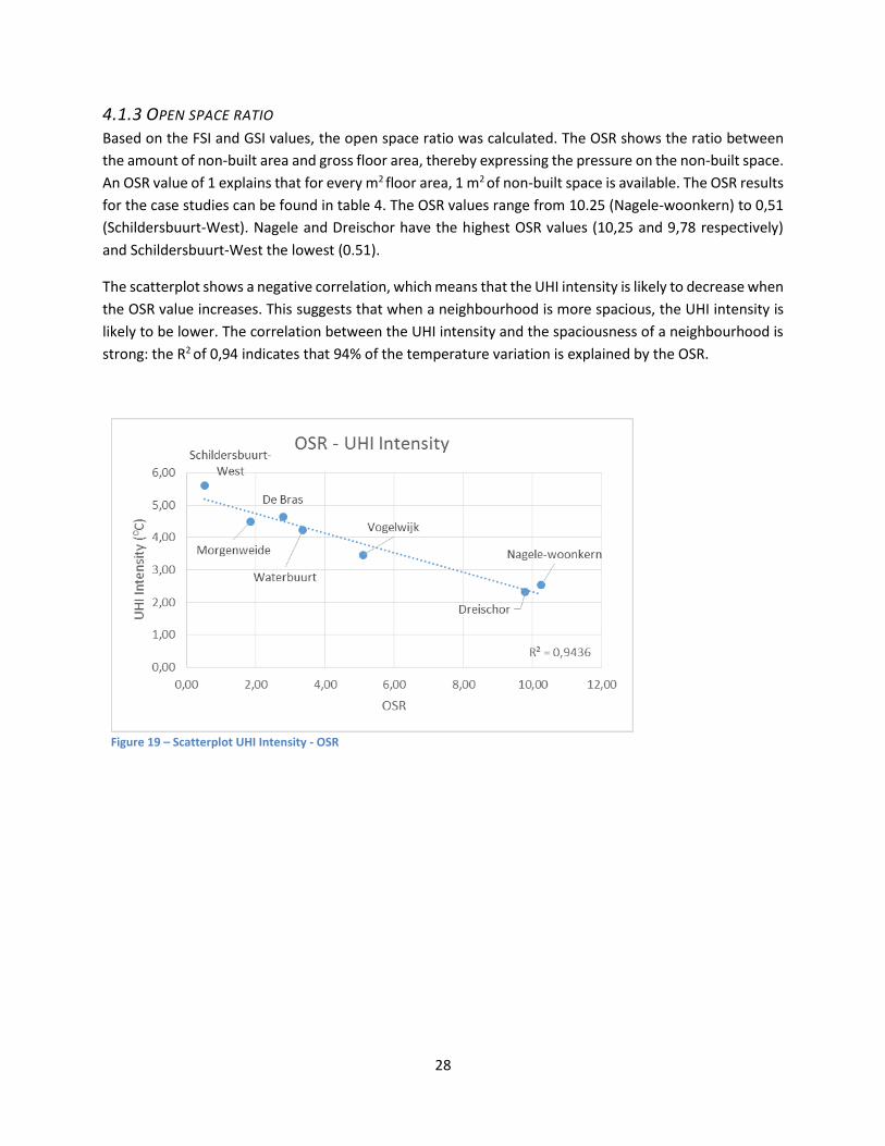
28

4.1.3 OPEN SPACE RATIO Based on the FSI and GSI values, the open space ratio was calculated. The OSR shows the ratio between

the amount of non-built area and gross floor area, thereby expressing the pressure on the non-built space.

An OSR value of 1 explains that for every m2 floor area, 1 m2 of non-built space is available. The OSR results

for the case studies can be found in table 4. The OSR values range from 10.25 (Nagele-woonkern) to 0,51

(Schildersbuurt-West). Nagele and Dreischor have the highest OSR values (10,25 and 9,78 respectively)

and Schildersbuurt-West the lowest (0.51).

The scatterplot shows a negative correlation, which means that the UHI intensity is likely to decrease when

the OSR value increases. This suggests that when a neighbourhood is more spacious, the UHI intensity is

likely to be lower. The correlation between the UHI intensity and the spaciousness of a neighbourhood is

strong: the R2 of 0,94 indicates that 94% of the temperature variation is explained by the OSR.

Figure 19 – Scatterplot UHI Intensity - OSR

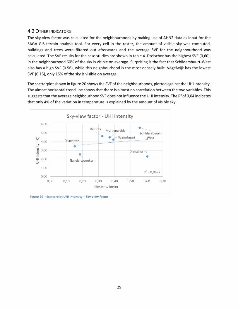
29

4.2 OTHER INDICATORS The sky-view factor was calculated for the neighbourhoods by making use of AHN2 data as input for the

SAGA GIS terrain analysis tool. For every cell in the raster, the amount of visible sky was computed,

buildings and trees were filtered out afterwards and the average SVF for the neighbourhood was

calculated. The SVF results for the case studies are shown in table 4. Dreischor has the highest SVF (0,60),

in the neighbourhood 60% of the sky is visible on average. Surprising is the fact that Schildersbuurt-West

also has a high SVF (0.56), while this neighbourhood is the most densely built. Vogelwijk has the lowest

SVF (0.15), only 15% of the sky is visible on average.

The scatterplot shown in figure 20 shows the SVF of the neighbourhoods, plotted against the UHI intensity.

The almost horizontal trend line shows that there is almost no correlation between the two variables. This

suggests that the average neighbourhood SVF does not influence the UHI intensity. The R2 of 0,04 indicates

that only 4% of the variation in temperature is explained by the amount of visible sky.

Figure 20 – Scatterplot UHI Intensity – Sky-view factor

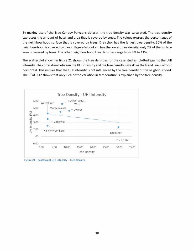
30

By making use of the Tree Canopy Polygons dataset, the tree density was calculated. The tree density

expresses the amount of base land area that is covered by trees. The values express the percentages of

the neighbourhood surface that is covered by trees. Dreischor has the largest tree density, 30% of the

neighbourhood is covered by trees. Nagele-Woonkern has the lowest tree density, only 2% of the surface

area is covered by trees. The other neighbourhood tree densities range from 3% to 11%.

The scatterplot shown in figure 21 shows the tree densities for the case studies, plotted against the UHI

intensity. The correlation between the UHI intensity and the tree density is weak, as the trend line is almost

horizontal. This implies that the UHI intensity is not influenced by the tree density of the neighbourhood.

The R2 of 0,12 shows that only 12% of the variation in temperature is explained by the tree density.

Figure 21 – Scatterplot UHI Intensity – Tree Density

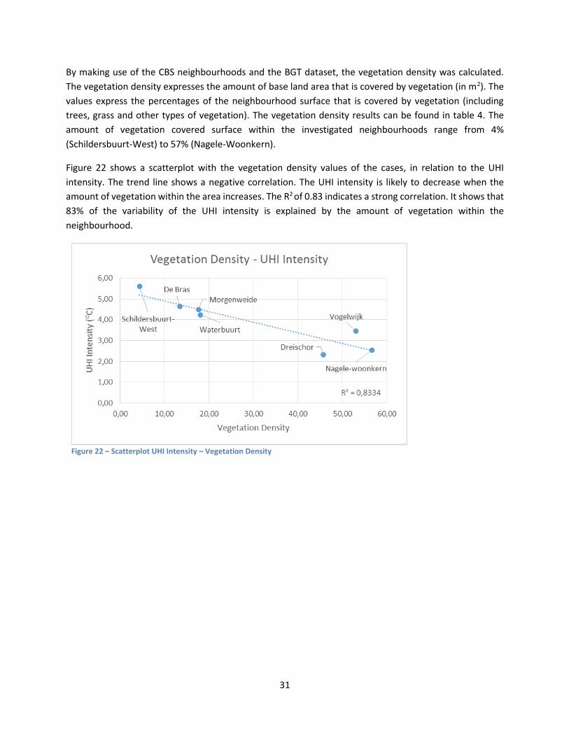
31

By making use of the CBS neighbourhoods and the BGT dataset, the vegetation density was calculated.

The vegetation density expresses the amount of base land area that is covered by vegetation (in m2). The

values express the percentages of the neighbourhood surface that is covered by vegetation (including

trees, grass and other types of vegetation). The vegetation density results can be found in table 4. The

amount of vegetation covered surface within the investigated neighbourhoods range from 4%

(Schildersbuurt-West) to 57% (Nagele-Woonkern).

Figure 22 shows a scatterplot with the vegetation density values of the cases, in relation to the UHI

intensity. The trend line shows a negative correlation. The UHI intensity is likely to decrease when the

amount of vegetation within the area increases. The R2 of 0.83 indicates a strong correlation. It shows that

83% of the variability of the UHI intensity is explained by the amount of vegetation within the

neighbourhood.

Figure 22 – Scatterplot UHI Intensity – Vegetation Density

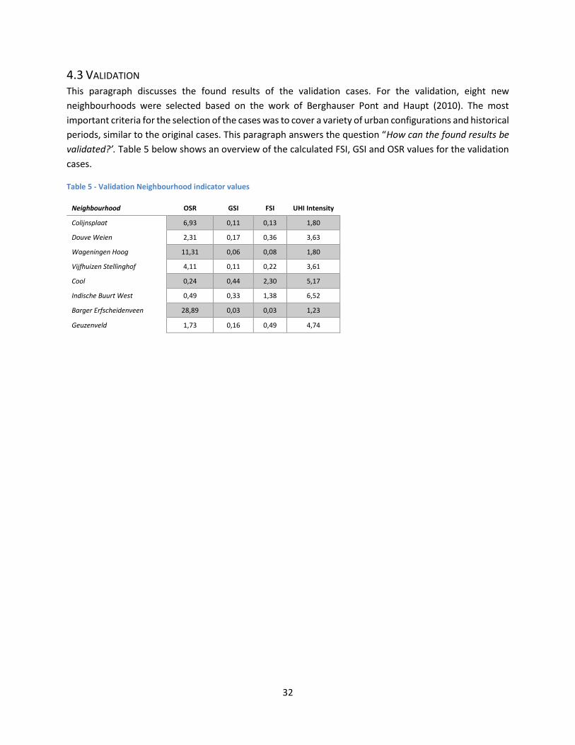
32

4.3 VALIDATION This paragraph discusses the found results of the validation cases. For the validation, eight new

neighbourhoods were selected based on the work of Berghauser Pont and Haupt (2010). The most

important criteria for the selection of the cases was to cover a variety of urban configurations and historical

periods, similar to the original cases. This paragraph answers the question “How can the found results be

validated?’. Table 5 below shows an overview of the calculated FSI, GSI and OSR values for the validation

cases.

Table 5 - Validation Neighbourhood indicator values

Neighbourhood OSR GSI FSI UHI Intensity

Colijnsplaat 6,93 0,11 0,13 1,80

Douve Weien 2,31 0,17 0,36 3,63

Wageningen Hoog 11,31 0,06 0,08 1,80

Vijfhuizen Stellinghof 4,11 0,11 0,22 3,61

Cool 0,24 0,44 2,30 5,17

Indische Buurt West 0,49 0,33 1,38 6,52

Barger Erfscheidenveen 28,89 0,03 0,03 1,23

Geuzenveld 1,73 0,16 0,49 4,74

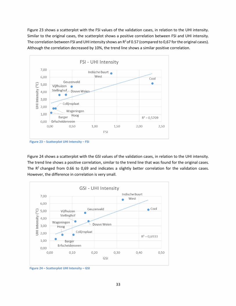
33

Figure 23 shows a scatterplot with the FSI values of the validation cases, in relation to the UHI intensity.

Similar to the original cases, the scatterplot shows a positive correlation between FSI and UHI intensity.

The correlation between FSI and UHI intensity shows an R2 of 0.57 (compared to 0,67 for the original cases).

Although the correlation decreased by 10%, the trend line shows a similar positive correlation.

Figure 23 – Scatterplot UHI Intensity – FSI

Figure 24 shows a scatterplot with the GSI values of the validation cases, in relation to the UHI intensity.

The trend line shows a positive correlation, similar to the trend line that was found for the original cases.

The R2 changed from 0.66 to 0,69 and indicates a slightly better correlation for the validation cases.

However, the difference in correlation is very small.

Figure 24 – Scatterplot UHI Intensity – GSI

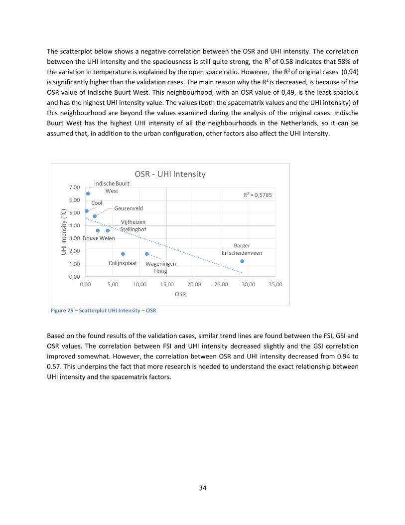
34

The scatterplot below shows a negative correlation between the OSR and UHI intensity. The correlation

between the UHI intensity and the spaciousness is still quite strong, the R2 of 0.58 indicates that 58% of

the variation in temperature is explained by the open space ratio. However, the R2 of original cases (0,94)

is significantly higher than the validation cases. The main reason why the R2 is decreased, is because of the

OSR value of Indische Buurt West. This neighbourhood, with an OSR value of 0,49, is the least spacious

and has the highest UHI intensity value. The values (both the spacematrix values and the UHI intensity) of

this neighbourhood are beyond the values examined during the analysis of the original cases. Indische

Buurt West has the highest UHI intensity of all the neighbourhoods in the Netherlands, so it can be

assumed that, in addition to the urban configuration, other factors also affect the UHI intensity.

Figure 25 – Scatterplot UHI Intensity – OSR

Based on the found results of the validation cases, similar trend lines are found between the FSI, GSI and

OSR values. The correlation between FSI and UHI intensity decreased slightly and the GSI correlation

improved somewhat. However, the correlation between OSR and UHI intensity decreased from 0.94 to

0.57. This underpins the fact that more research is needed to understand the exact relationship between

UHI intensity and the spacematrix factors.

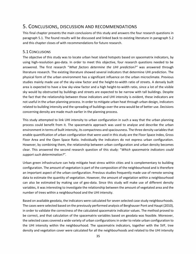
35

5. CONCLUSIONS, DISCUSSION AND RECOMMENDATIONS This final chapter presents the main conclusions of this study and answers the four research questions in

paragraph 5.1. The found results will be discussed and linked back to existing literature in paragraph 5.2

and this chapter closes of with recommendations for future research.

5.1 CONCLUSIONS The objective of this study was to locate urban heat island hotspots based on spacematrix indicators, by

using high-resolution geo-data. In order to meet this objective, four research questions needed to be

answered. The first research “What factors determine the UHI prediction?” was answered through

literature research. The existing literature showed several indicators that determine UHI prediction. The

physical form of the urban environment has a significant influence on the urban microclimate. Previous

studies mainly made use of the sky-view factor and the height-to-width ratio of streets. A densely built

area is expected to have a low sky-view factor and a high height-to-width ratio, since a lot of the visible

sky would by obstructed by buildings and streets are expected to be narrow with tall buildings. Despite

the fact that the relationship between those indicators and UHI intensity is evident, these indicators are

not useful in the urban planning process. In order to mitigate urban heat through urban design, indicators

related to building intensity and the spreading of buildings over the area would be of better use. Decisions

concerning density are made much earlier in the planning process.

This study attempted to link UHI intensity to urban configuration in such a way that the urban planning

process could benefit from it. The spacematrix approach was used to analyse and describe the urban

environment in terms of built intensity, its compactness and spaciousness. The three density variables that

enable quantification of urban configuration that were used in this study are the Floor Space Index, Gross

Floor Area and the Open Space Ratio. Individually the indicators do not express urban configuration.

However, by combining them, the relationship between urban configuration and urban density becomes

clear. This answered the second research question of this study: “Which spacematrix indicators could

support such determination?”.

Urban green infrastructure can help mitigate heat stress within cities and is complementary to building

configuration. The amount of vegetation is part of the composition of the neighbourhood and is therefore

an important aspect of the urban configuration. Previous studies frequently made use of remote sensing

data to estimate the quantity of vegetation. However, the amount of vegetation within a neighbourhood

can also be estimated by making use of geo-data. Since this study will make use of different density

variables, it was interesting to investigate the relationship between the amount of vegetated area and the

number of trees within a neighbourhood and the UHI intensity.

Based on available geodata, the indicators were calculated for seven selected case study neighbourhoods.

The cases were selected based on the previously performed analysis of Berghauser Pont and Haupt (2010),

in order to validate the correctness of the calculated spacematrix indicator values. The method proved to

be correct, and that calculation of the spacematrix variables based on geodata was feasible. Moreover,

the selected cases covered a wide variety of urban configurations in order to relate urban configuration to

the UHI intensity within the neighbourhood. The spacematrix indicators, together with the SVF, tree

density and vegetation cover were calculated for all the neighbourhoods and related to the UHI intensity

36

temperature. This answered the third research question “How do the spacematrix indicators relate to UHI

intensity in neighbourhoods?”.

In general, the following assumptions can be made based on the results of this study:

The UHI intensity increases when the amount of floor space within a neighbourhood increases.

The UHI intensity increases when the amount of built-up area within a neighbourhood

increases.

The UHI intensity decreases when the spaciousness of a neighbourhood increases.

There seems to be no correlation between the average sky-view factor of a neighbourhood

and the UHI intensity.

There seems to be no correlation between the tree density of a neighbourhood and the UHI

intensity.

The UHI intensity decreases when the amount of vegetation within a neighbourhood

increases.

After the calculations of the indicators for the selected neighbourhoods, the results needed to be

validated. This was done by investigating eight new neighbourhoods, with similar urban configurations

compared to the original case studies. The validation showed that the validation cases display similar trend

lines and correlations. The correlation between FSI and UHI intensity decreased slightly and the GSI

correlation improved. However, the correlation between OSR and UHI intensity decreased from 0.94 to

0.57. This underpins the fact that more research is needed to understand the exact relationship between

UHI intensity and the spacematrix factors.

5.2 DISCUSSION Although further research is required, the spacematrix indicators prove to be applicable for the purposes

of an early stage UHI prediction regarding design concepts of urban configuration. This paragraph

discusses the found results in relation to existing literature, the use and limitations of the method used in

this study and the accuracy of the used data.

5.2.1 RESULTS As became clear in the literature review, previous studies on urban configuration in relation the urban

heat, mainly made use of sky-view factors and height-to-width ratios. The effect of building configuration

on UHI intensity is rather complex. The complexity is caused by counteracting effects, that occur at

different times (Theeuwes, 2015). Shadowing during the day caused by narrow streets or high buildings

results in lower temperatures. However, the heat that was stored by the buildings during the day is

trapped during the night because of the narrowness. High building densities are often assumed to have a

negative influence on the extent of UHIs. The results found in this study justify those assumptions, as far

as built intensity, coverage and spaciousness of an area are concerned. In agreement with literature, the

found negative correlation with the open space ratio suggests that the more open an area is

(corresponding to a high sky-view factor and low height-to-width ratio), the lower the expected UHI

intensity is. Based on the results found in this study, cooler temperatures arise in more spacious

neighbourhoods. The assumption is that the unbuilt space within a neighbourhood is partly used for

37

vegetation and other heat mitigating measures. Moreover, both the amount of floor space and the ratio

between built area and the size of the neighbourhood seem to have a positive correlation to the UHI

intensity. However, literature explains that the effects of street geometry on temperature are

counteracting. This may be the reason why the amount of floor space and or the coverage of an area

correlate less with temperature, as compared to the spaciousness. Spaciousness within an area provides

more space for vegetation, less obstruction by wind and wider streets.

Rather surprising is the fact that the found results regarding the sky-view factor do not correlate with the

UHI intensity. This does not agree with the findings of previous studies. The exact reason why this is the

case is unknown, but it may be caused by the fact that the SAGA GIS tool did not perform the SVF analysis

correctly. This assumption is supported by the fact that the SVF for the ‘Schildersbuut-West’ is high (0.56)

while this is the most densely built neighbourhood. Furthermore, the SVF of Vogelwijk is quite low (0,15),

while the neighbourhood is fairly spacious with an OSR value of 5.11.

Also the tree density indicator did not show any correlation to UHI intensity. The choice to include and

calculate the tree density was an experiment, inspired by the availability of geodata. Literature states that

trees influence the temperature in their immediate vicinity. With the availability of the Tree Canopy

Polygon dataset, the possibility of investigating the influence of trees on neighbourhood UHI intensity

became possible. However, no correlation was found.

The vegetation density that was calculated based on BGT vegetation data showed a high correlation with

UHI intensity. This supports the general findings of existing literature: an increase in the amount of

vegetation lowers the temperature by reducing both the air and surface temperature within the urban

environment. The results found in this research are in accordance with those findings. The negative

correlation between vegetation density and UHI intensity, confirms that more vegetation within a

neighbourhood is correlated with a lower temperature.

5.2.2 USE AND LIMITATIONS OF THE USED METHOD This study shows that there is a basic relation between built density, urban configuration and UHI intensity.

The impact of high buildings, narrow streets and densely built urban landscapes on urban temperature is

somewhat intuitively understood and is studied by many researchers. However, for urban design, the

urban planning practice would benefit from a method to quantify urban configuration and density. By the

investigation of the spacematrix indicators, a general trend between urban heat and these indicators

became visible. Especially the open space ratio and UHI intensity showed a strong correlation. This

suggests that out of two design plans with the same amount of floor space, but with different degrees of

spaciousness, the more spacious design would perform better regarding urban heat performance.

Although more research into this topic is necessary, the found results suggest that a higher more spacious

building configuration would perform better than a lower compact one. The spacematrix indicators can be

used to understand the different consequences of urban configuration on urban heat, and therefore create

a better understanding of the influence of urban design on the quality of urban environments. Urban

design has a huge influence on the urban climate. The spacematrix indicators can help urban planners and

decision-makers to make the right choices early in the planning process to help mitigate urban heat stress.

The influence of the governmental sector on urban climate adaption is large, and by incorporating density

38

guidelines in urban zoning schemes, master plans and other public space plans, climate adaption can be

considered early in the planning process. New design concepts need to provide insights into the ratio

between built and unbuilt space and the desired amount of floor space, in order to estimate the impact

on UHI intensity. Moreover, on the basis of freely available geodata, existing neighbourhoods can be

analysed quickly with the method proposed in this study. In this manner, an early warning for their

sensitivity to the UHI effect can be established. However, this does not mean that there is a simple formula

for creating an urban design that will completely mitigate urban heat. More factors are of influence, for

instance the presence of vegetation and the used built materials. The spacematrix indicators can create

awareness, but it is not guaranteed that the UHI intensity is decreased by the application of the full

potential of the indicators. In other words, creating optimal density conditions within a design plan is the

first step towards mitigation of urban heat. The cumulative effect of small-scale interventions, such as the

greening of public spaces, cannot be ignored. Such interventions still contribute greatly to the reduction

of the UHI effect.

This study focussed on the neighbourhood scale, mainly because the temperature data was available at

this scale. However, the mitigation of urban heat involves interventions at different scale levels

(Lenzholzer, 2013) and these scales cross administrative borders. The choice for the neighbourhood scale

resulted in some limitations. The fact that a neighbourhood has a certain FSI, GSI or OSR value, does not

mean that the complete area has a uniform density. In fact, the larger the area is that the spacematrix

values are calculated for, the more likely it is that the area is heterogeneous. However, small-scale

interventions should be targeted at those locations that are more densely built. This makes the calculations

of spacematrix values at neighbourhood level unsuitable for localization of small target areas. The

sensitivity of the outcomes of this study to scale can be an interesting topic for future research. The

spacematrix values can be calculated for a variety of land units, like acre or hectare. By analysing such

kinds of sampling strategies, the smaller scale effects of urban configuration on UHI intensity can be tested

and related back to neighbourhood scale.

5.2.3 ACCURACY OF THE USED DATA The data that was used in this study was not error free and could not be used without encountering some

problems. This paragraph provides an overview of some of the problems that were encountered during

this study.

When the CBS neighbourhoods dataset was clipped with the BAG buildings, the neighbourhood

borders cut right through buildings. This led to building shreds. Buildings smaller than 1 m2 had to

be filtered out.

By making a combination between the AHN2 dataset and the BAG buildings in order to estimate

the building height, a problem in concerning actuality of the data arose. Buildings that were

demolished after 2007 (the year that the AHN2 started to be collected) still got a height value,

since the AHN2 data still contained that building. The opposite problem was encountered for

buildings that were built after 2007: no height value was assigned to these buildings.

The BGT dataset is provided via the PDOK data portal, in a GML data format. However, the GML

could not be loaded into ArcMap. The exact reason why is unknown, but ESRI also couldn’t solve

39

the problem. In the end, the BGT data had to be downloaded from a PostgreSQL server, provided

by data.extractnl.nl.

The metadata of the BAG dataset is not well documented. This caused some confusion about the

meaning of the attribute values. The BAG buildings dataset contains an attribute, called “aantal

ver”. Intuitively, this can be understood as the number of stories of a building. However, this

attribute contained information about the number of properties within the building. This was not

documented. Furthermore, some numeric values within the BAG were classified as string

attributes.

5.3 RECOMMENDATIONS FOR FUTURE RESEARCH The research related to urban heat islands and the urban microclimate has been expanding rapidly and a

lot has been researched already. This study resulted in an early UHI warning regarding the change of

cityscape lay-outs. However, the complexity of the influence that cities have on their environment offers

plenty of opportunities for further studies. This paragraph discusses the recommendations for future

research.

In this study, the relationship between urban configuration and urban heat island intensity was examined.

The first step in relating urban heat to the spacematrix density variables was made by the study of seven

neighbourhoods. Based on the results, the relationship between the spacematrix indicators and UHI

intensity appears to be significant. Chapter two shows that existing literature has studied the relationship

between urban configuration and urban heat islands, but the interaction between building configuration

and the extent of urban heat is still not fully understood. In order to generalise the results found in this

study, more cases need to be analysed. The next step in this research could consist of the calculation of

the FSI, GSI and OSR values for all the neighbourhoods in the Netherlands. By making use of the possibilities

of programming, calculation of the spacematrix variables could be automated and computed nationwide.

This would enhance the potential for predicting the UHI intensity in neighbourhoods, based on their

spacematrix values. Besides, the statistical significance of the results of this study will change because of

the higher number of analysed cases. An alternative option would be to research the sensitivity of the

spacematrix indicators to different scale levels.

Another suggestion for further research would be to investigate the possible impact of the found results

of this study on the urban planning practice. A significant contribution to the planning process would be

to investigate in what manner mitigation and adaption of urban heat are currently institutionalised within

municipalities and how urban planners and decision-makers could benefit from urban climate research.

The question arises, is neighbourhood level the most useful scale? While conducting this research, it

became apparent that the gap between research and the application of adaption and mitigation strategies

is large at some points. By getting a better understanding of how the planning process works, the gap

between science and practice can be bridged.

40

REFERENCES Albers, R. A. W., Bosch, P. R., Blocken, B., van Den Dobbelsteen, A. A. J. F., van Hove, L. W. A., Spit, T. J.

M., Rovers, V. (2015). Overview of challenges and achievements in the climate adaptation of cities and in the Climate Proof Cities program Building and Environment (Vol. 83, pp. 1-10).

Alcoforado, M.-J., Andrade, H., Lopes, A., & Vasconcelos, J. (2009). Application of climatic guidelines to urban planning. The example of Lisbon (Portugal). Landscape and Urban Planning, 90(1-2), 56-65. doi: 10.1016/j.landurbplan.2008.10.006

Armson, D., Stringer, P., & Ennos, A. R. (2012). The effect of tree shade and grass on surface and globe temperatures in an urban area. Urban Forestry & Urban Greening, 11(3), 245-255. doi: 10.1016/j.ufug.2012.05.002

Berghauser Pont, M., & Haupt, P. (2010). Spacematrix : space, density and urban form: Rotterdam, NL: NAi Publishers.

Bourbia, F., & Awbi, H. B. (2004a). Building cluster and shading in urban canyon for hot dry climate: Part 1: Air and surface temperature measurements. Renewable Energy, 29(2), 249-262. doi: http://dx.doi.org/10.1016/S0960-1481(03)00170-8

Bourbia, F., & Awbi, H. B. (2004b). Building cluster and shading in urban canyon for hot dry climate: Part 2: Shading simulations. Renewable Energy, 29(2), 291-301. doi: http://dx.doi.org/10.1016/S0960-1481(03)00171-X

Bourbia, F., & Boucheriba, F. (2010). Impact of street design on urban microclimate for semi arid climate (Constantine). Renewable Energy, 35(2), 343-347. doi: 10.1016/j.renene.2009.07.017

Bowler, D. E., Buyung-Ali, L., Knight, T. M., & Pullin, A. S. (2010). Urban greening to cool towns and cities: A systematic review of the empirical evidence. Landscape and Urban Planning, 97(3), 147-155. doi: 10.1016/j.landurbplan.2010.05.006

CBS. (n.d.). Begrippen. Retrieved 19-3-2016, 2016, from https://www.cbs.nl/nl-nl/onze-diensten/methoden/begrippen?tab=b#id=buurt

Chang, C.-R., & Li, M.-H. (2014). Effects of urban parks on the local urban thermal environment. Urban Forestry & Urban Greening, 13(4), 672-681. doi: 10.1016/j.ufug.2014.08.001

Döpp, S., Klok, L., Jacobs, C., Kleerekoper, L., & Uittenbroek, C. J. (2011). Kennismontage Hitte en Klimaat in de Stad.

Emmanuel, R., & Loconsole, A. (2015). Green infrastructure as an adaptation approach to tackling urban overheating in the Glasgow Clyde Valley Region, UK. Landscape and Urban Planning, 138, 71-86. doi: 10.1016/j.landurbplan.2015.02.012

Fernandez, A., & Mozas, J. ( 2004). Densidad. Density. Vitoria-Gasteiz. Fina, S., Krehl, A., Siedentop, S., Taubenböck, H., & Wurm, M. (2014). Getting Closer! New Ways of

Integrating Geodata, Statistics and Remote Sensing to Analyze and Visualize Urban Structures Using Density Surfaces and -Profiles. Raumforschung und Raumordnung, 72(3), 179-194. doi: 10.1007/s13147-014-0279-6

Forsyth, A. (2003). Measuring Density: Working Definitions for Residential Density and Building Intensity (Vol. Number 8). Twin Cities: Design Center for American Urban Landscape Design Brief.

Futcher, J. A. (2008). Ice tea city. Paper presented at the 25th Conference on Passive and low Energy Architecture Dublin.

Gillner, S., Vogt, J., Tharang, A., Dettmann, S., & Roloff, A. (2015). Role of street trees in mitigating effects of heat and drought at highly sealed urban sites. Landscape and Urban Planning. doi: 10.1016/j.landurbplan.2015.06.005

Gemeente Den Haag (1996). Bestemmingsplan Vogelwijk. Den Haag: Gemeente Den Haag. Gemeente Den Haag (2013 ). Bestemmingsplan Ypenburg De Bras. Den Haag: Gemeente Den Haag.

41

Gemeente Den Haag (2015). Bestemmingsplan Ypenburg Toelichting. Den Haag: Retrieved from http://www.denhaag.nl/home/bewoners/stadsdelen-en-wijken/leidschenveen-ypenburg/to/Ypenburg-3.htm.

Holtslag, A. A. M., Ronda, R. J., Steeneveld, G. J., Heusinkveld, B. G., & Harst, M. v. d. (2013). Summer in the City—Forecasting and Mapping Human Thermal Comfort in Urban Areas.

Hotkevica, I. (2013). Green elements in street canyons : research by design for heat mitigation and thermal comfort in urban areas: [S.l., NL: s.n.].

Johansson, E. (2006). Influence of urban geometry on outdoor thermal comfort in a hot dry climate: A study in Fez, Morocco. Building and Environment, 41(10), 1326-1338. doi: http://dx.doi.org/10.1016/j.buildenv.2005.05.022

Keeley, M. (2011). The Green Area Ratio: an urban site sustainability metric. Journal of Environmental Planning and Management, 54(7), 937-958. doi: 10.1080/09640568.2010.547681

Kleerekoper, L., van Esch, M., & Salcedo, T. B. (2012). How to make a city climate-proof, addressing the urban heat island effect. Resources, Conservation & Recycling, 64, 30-38. doi: 10.1016/j.resconrec.2011.06.004

Lenzholzer, S., & Lahr, M. (2013). Het weer in de stad : hoe ontwerp het stadsklimaat bepaalt: Rotterdam, NL: nai010 uitgevers.

Lin, W., Yu, T., Chang, X., Wu, W., & Zhang, Y. (2015). Calculating cooling extents of green parks using remote sensing: Method and test. Landscape and Urban Planning, 134, 66-75. doi: http://dx.doi.org/10.1016/j.landurbplan.2014.10.012

Meijer, M., Rip, F., Benthem, R. v., & Clement, J. (2015). Boomkronen afleiden uit het Actueel Hoogtebestand Nederland : kwaliteitsaspecten rondom het geautomatiseerd in kaart brengen van bomen op basis van het AHN2-bestand. Wageningen: Alterra Wageningen UR.

Mullaney, J., Lucke, T., & Trueman, S. J. (2015). A review of benefits and challenges in growing street trees in paved urban environments. Landscape and Urban Planning, 134, 157-166. doi: http://dx.doi.org/10.1016/j.landurbplan.2014.10.013

Noordoostpolder, G. (2010). Bestemmingsplan Nagele - Ontstaansgeschiedenis. Noordoostpolder: Gemeente Noordoostpolder Retrieved from http://www.ruimtelijkeplannen.nl/documents/NL.IMRO.0171.BP00482-VO01/t_NL.IMRO.0171.BP00482-VO01_2.3.html#begin.

Norton, B. A., Coutts, A. M., Livesley, S. J., Harris, R. J., Hunter, A. M., & Williams, N. S. G. (2015). Planning for cooler cities: A framework to prioritise green infrastructure to mitigate high temperatures in urban landscapes. Landscape and Urban Planning, 134, 127-138. doi: 10.1016/j.landurbplan.2014.10.018

Oke, T. R. (1981). Canyon geometry and the nocturnal urban heat island: Comparison of scale model and field observations. Journal of Climatology, 1(3), 237-254. doi: 10.1002/joc.3370010304

Oorschot, L. (2015). VINEX: Ypenburg Revisited. Retrieved 10-4-2016, 2016, from http://www.haacs.nl/vinex-ypenburg-revisited/

Peng, S., Piao, S., Ciais, P., Friedlingstein, P., Ottle, C., Bréon, F.-M., . . . Myneni, R. B. (2012). Surface urban heat island across 419 global big cities. Environmental science & technology, 46(2), 696. doi: 10.1021/es2030438

Ren, C., Ng, E. Y. y., & Katzschner, L. (2011). Urban climatic map studies: a review International Journal of Climatology (Vol. 31, pp. 2213-2233). Chichester, UK.

Rovers, V., Bosch, P. R., & Albers, R. A. W. (2014). Eindrapport Climate proof cities: [S.l.], NL: Programme Office Knowledge for Climate.

Silvera Seamans, G. (2012). Mainstreaming the environmental benefits of street trees. Urban Forestry & Urban Greening. doi: 10.1016/j.ufug.2012.08.004

Song, J., & Li, X. (2010). A study on the cooling effects of greenery on the surrounding areas by computer simulation for green built environment (Vol. 6330, pp. 653-661).

42

Steeneveld, G. J., Koopmans, S., Heusinkveld, B. G., Van Hove, L. W. A., & Holtslag, A. A. M. (2011). Quantifying urban heat island effects and human comfort for cities of variable size and urban morphology in the Netherlands. Journal of Geophysical Research: Atmospheres, 116(D20), n/a-n/a. doi: 10.1029/2011jd015988

Taleghani, M., Kleerekoper, L., Tenpierik, M., & van Den Dobbelsteen, A. (2015). Outdoor thermal comfort within five different urban forms in the Netherlands. Building and Environment, 83, 65-78. doi: 10.1016/j.buildenv.2014.03.014

Tan, M., & Li, X. (2013). Integrated assessment of the cool island intensity of green spaces in the mega city of Beijing. International Journal of Remote Sensing, 34(8), 3028-3043. doi: 10.1080/01431161.2012.757377

Theeuwes, N. E. (2015). Urban heat : natural and anthropogenic factors influencing urban air temperatures: Wageningen, NL: Wageningen University.

Unger, J., Savić, S., & Gál, T. (2011). Modelling of the Annual Mean Urban Heat Island Pattern for Planning of Representative Urban Climate Station Network. Advances in Meteorology, 2011. doi: 10.1155/2011/398613

van Esch, M., de Bruin-Hordijk, T., & Duijvestein, K. (2007). The influence of building geometry on the physical urban climate: a revival of light, air and space’. Paper presented at the The 24th Conference on Passive and Low Energy Architecture, Singapore.

van Hove, L. W. A., Jacobs, C. M. J., Heusinkveld, B. G., Elbers, J. A., van Driel, B. L., & Holtslag, A. A. M. (2015). Temporal and spatial variability of urban heat island and thermal comfort within the Rotterdam agglomeration. Building and Environment, 83, 91-103. doi: 10.1016/j.buildenv.2014.08.029

van Nes, A., Berghauser Pont, M., & Mashhoodi, B. (2012). Combination of space syntax with spacematrix and the mixed use index: The Rotterdam South test case. . Paper presented at the Space Syntax Symposium, Santiago.

Yang, X., & Li, Y. (2015). The impact of building density and building height heterogeneity on average urban albedo and street surface temperature. Building and Environment, 90, 146-156. doi: 10.1016/j.buildenv.2015.03.037

Žiga, K., Klemen, Z., & Kristof, O. (2011). Sky-View Factor as a Relief Visualization Technique. Remote Sensing, 3(2), 398-415. doi: 10.3390/rs3020398

Zinzi, M., & Agnoli, S. (2012). Cool and green roofs. An energy and comfort comparison between passive cooling and mitigation urban heat island techniques for residential buildings in the Mediterranean region. Energy and Buildings, 55, 66-76. doi: http://dx.doi.org/10.1016/j.enbuild.2011.09.024

43

APPENDIX 1: TABLE OF CONTENTS DVD The DVD that accompanies this thesis report contains the following information: Documents

• Final thesis report (Word, PDF) • All cited literature (Endnote library)

Presentations

• Midterm presentation (PDF) • Final presentation (PDF)

Data (for all case studies)

• BGT • AHN2 • BAG • Tree Canopy Polygons • Temperature Data

Applications

• ArcMap Models Figures and maps

• Figures report