Using Augmented Measurements to Improve theConvergence of ICP

Jacopo Serafin, Giorgio Grisetti

Dept. of Computer, Control and Management Engineering,Sapienza University of Rome, Via Ariosto 25, I-00185, Rome, Italy

serafin,grisetti@dis.uniroma1.it

Abstract. Point cloud registration is an essential part for many roboticsapplications and this problem is usually addressed using some of the ex-isting variants of the Iterative Closest Point (ICP) algorithm. In thispaper we propose a novel variant of the ICP objective function which isminimized while searching for the registration. We show how this newfunction, which relies not only on the point distance, but also on thedifference between surface normals or surface tangents, improves the reg-istration process. Experiments are performed on synthetic data and realstandard benchmark datasets, showing that our approach outperformsother state of the art techniques in terms of convergence speed and ro-bustness.

Keywords: Point Cloud Registration · ICP · Surface Normals

1 Introduction

Registering two point clouds is a building block of many robot applications suchas simultaneous localization and mapping (SLAM), object recognition and de-tection, augmented reality and many others. This problem is commonly solvedby variants of the Iterative Closest Point (ICP) algorithm proposed by Besl andMcKay [1]. ICP tries to find a transformation that minimizes the distance ofa set of corresponding points in the two clouds. At each iteration ICP refinesthe estimate of the transformation by alternating a search and an optimizationroutine. Given the current transform, the search looks for corresponding pointsin the two clouds. The optimization computes the transformation that resultsin the minimum distance between the corresponding points found by the searchstep. ICP is a very successful scheme and several variants of increasing perfor-mances have been proposed. If the correspondences are free from outliers andthe measurements are affected by low noise, the transformation can be founddirectly by applying the Horn formula [3].

The whole concept at the base of ICP is that, at each iteration, an improvedtransformation with respect to the previous one is found. Such a transformationrepresents the new initial guess for the heuristic used to find the correspondencesand allows to determine better associations at the next iteration. Accordingly, re-searchers focused on seeking for heuristics that provide “good” correspondences.

The original idea of picking up the closest points [1] has been progressivelyrefined to consider features, curvature and other characteristics of the points.Pomerlau et al. [5] provided an excellent overview on these different variants.

ICP and its variants require multiple iterations because it does not existan heuristic that provides the exact correspondences. Since the optimizationrequires linear time in the number of correspondences, the bottleneck of thecomputation is represented by the heuristic that has to compute them.

The main drawback of ICP in its original formulation is the assumption thatthe points in the two surfaces are exactly the same. This is clearly not trueas the point clouds are obtained by sampling a set of points from the surfaceobserved by the sensor. If the observer position changes, the chances that twopoints in the clouds are the same is very low. This is particularly evident atlow sampling resolutions. Aware of this aspect, Magnusson et al. [4] proposedto approximate the surface with a set of Gaussians capturing the local statisticsof the surface in the neighborhood of a point. In that representation, calledthe Normal Distrubution Transform (NDT), the correspondence search uses theMahalanobis distance instead of the Euclidean one and the optimization tries tominimize it.

Similarly, Segal et al [6] proposed a refined version of ICP called GeneralizedICP (GICP). The core idea behind this algorithm is to account for the shape ofthe surface which surrounds a point by approximating it with a planar patch.In the optimization, two corresponding patches are aligned onto each other, ne-glecting the error along their tangent direction. This can be straightforwardlyimplemented by minimizing the Mahalanobis distance of corresponding points,where the covariance matrix of a measurement is forced to have the shape of adisk aligned with the sampled surface. Thanks to the better rejection of falsecorrespondences based on the surface normal cue and the more realistic objec-tive function, NDT and GICP exhibit a substantially more stable convergencebehavior.

In fact, within ICP and its variants, the optimization and the correspondencesearch are not independent. If the optimization is robust to outliers and exhibitsa smooth behavior, the chances that it finds a better solution at the subsequentstep increases. In this way an improvement is obtained at each iteration untila good solution is found. Despite NDT and GICP, the authors are unaware ofother methods that improve the objective function.

Since point clouds are the effects of sampling a surface, the local character-istics of this surface play a role in the optimization. From this point of view, theobjective function has to express some distance between surface samples, and theoptimization algorithm has to determine the optimal alignment between thesetwo set of samples. A surface sample, however, is not fully described just by 3Dpoints, but it requires additional cues like the surface normal, the curvature and,potentially, the direction of the edge. Both NDT and GICP minimize a distancebetween corresponding points, while they neglect additional cues that can indeedplay a role in determining the transformation and in rejecting outliers.

In this paper we propose a novel variant of the objective function which isoptimized while searching for the transformation. This function depends not onlyon the relative point distance, but also on the difference between surface normalsor tangents in case the point lies on an edge. We provide an iterative form for theoptimization routine and we show through experiments performed on syntheticdata and standard benchmark datasets that our approach outperforms otherstate of the art techniques, both in terms of convergence speed and robustness.

2 ICP

The problem of registering two point clouds consists in finding the rotationand the translation that maximizes the overlap between the two clouds. Moreformally, let Pr = pr

1:Nr and Pc = pc1:Nc be the two set of points, we want to

find the transformation T∗ that minimizes the distance between correspondingpoints in the two scenes:

T∗ = argminT

∑C

χ2ij︷ ︸︸ ︷(

pci −T⊕ pr

j

)TΩij

(pci −T⊕ pr

j

)︸ ︷︷ ︸eij(t)

. (1)

In Eq. 1 the symbols have the following meaning:

– T is the transform that is updated at each step i of the iterative algorithmwith the one found at iteration i− 1;

– Ωij is an information matrix that takes into account the noise properties ofthe sensor or of the surface;

– C = 〈i, j〉1:M is a set of correspondences between points in the two clouds.〈i, j〉 ∈ C means that the point pr

j in the cloud Pr corresponds to the pointpci in the cloud Pc;

– eij(t) is the error function that computes the distance between the pointpci and the corresponding point pr

j in the other cloud after applying thetransformation T;

– χ2ij is the Ωij-norm of the error eij(t);

– ⊕ is an operator that applies the transformation T to a point p. If we usethe homogeneous notation for transformations and points, ⊕ reduces to thematrix-vector product.

In general, the correspondences between two point clouds are not known. How-ever, in presence of a good approximation for the initial transform, they canbe “guessed” through some heuristic like nearest neighbour. In its most gen-eral formulation, ICP iteratively refines an initial transform T by searching forcorrespondences and finding the solution of Eq. 1. Such a new transformationis then used in order to compute the new correspondences. Eq. 1 describes theobjective function used in the optimization of ICP, NDT and GICP. In the caseof ICP, Ωij is a diagonal matrix potentially scaled with a weight representing

the confidence about the correctness of a correspondence. NDT computes thecovariances Σi directly from the point cloud and it measures the distances byusing the mean of the Gaussians rather than the points as shown in Eq. 2.

T∗ = argminT

∑C

(µci −T⊕ pr

j

)TΣ−1i

(µci −T⊕ pr

j

). (2)

In GICP, Ωij = Σ−1i depends only on the ith point pci and its neighborhood.

The covariance Σi is enforced to have a disk shape and to lie on the surface fromwhere pc

i was sampled. In all cases, the difference pci−T⊕pr

j is a 3D vector thatmeasures the offset between two 3D points and the domain of the error functionis <3.

Since an increase in the dimensionality of the points makes the whole systemmore observable, less correspondences are required for the optimization process.By characterizing each point with other quantities to which a transform canbe applied, we can achieve such an increase in the dimensionality. We propose,for this reason, the use of normals for quasi-planar regions and/or tangents forregions of high curvature.

3 Extended ICP

In this section we describe the extension of the model of ICP in order to consideralso normals and tangents of the surface. We first illustrate the general conceptand, subsequently, we focus on the case in which a local surface has either anormal, a tangent or none of the two. We conclude the section by sketching analgorithm to carry on the optimization.

3.1 Extending the Measurements

Let ni be the normal of a point pi belonging to a certain surface, and τ i itstangent if the point is part of an edge, we can then extend Eq. 1 as follows:

T∗ = argminT

∑C

(pci −T⊕ pr

j

)TΩpij

(pci −T⊕ pr

j

)+

∑C

(nci −T⊕ nr

j

)TΩnij

(nci −T⊕ nr

j

)+

∑C

(τ ci −T⊕ τ r

j

)TΩτij

(τ ci −T⊕ τ r

j

).

(3)

Here nci , nr

j and Ωnij represent respectively the normal of the point pc

i andpri, and the information matrix of the correspondence among the two normals.

Similarly, τ ci , τ

rj and Ωτ

ij are the tangents and the information matrix of thecorrespondence among the two tangents. We recall that, if T is a transformationdescribed by a rotation matrix R and a translation vector t, the ⊕ operator hasdifferent definitions depending on its arguments:

T⊕ x =

R · x + t if x is a point

R · x if x is a tangent or a normal(4)

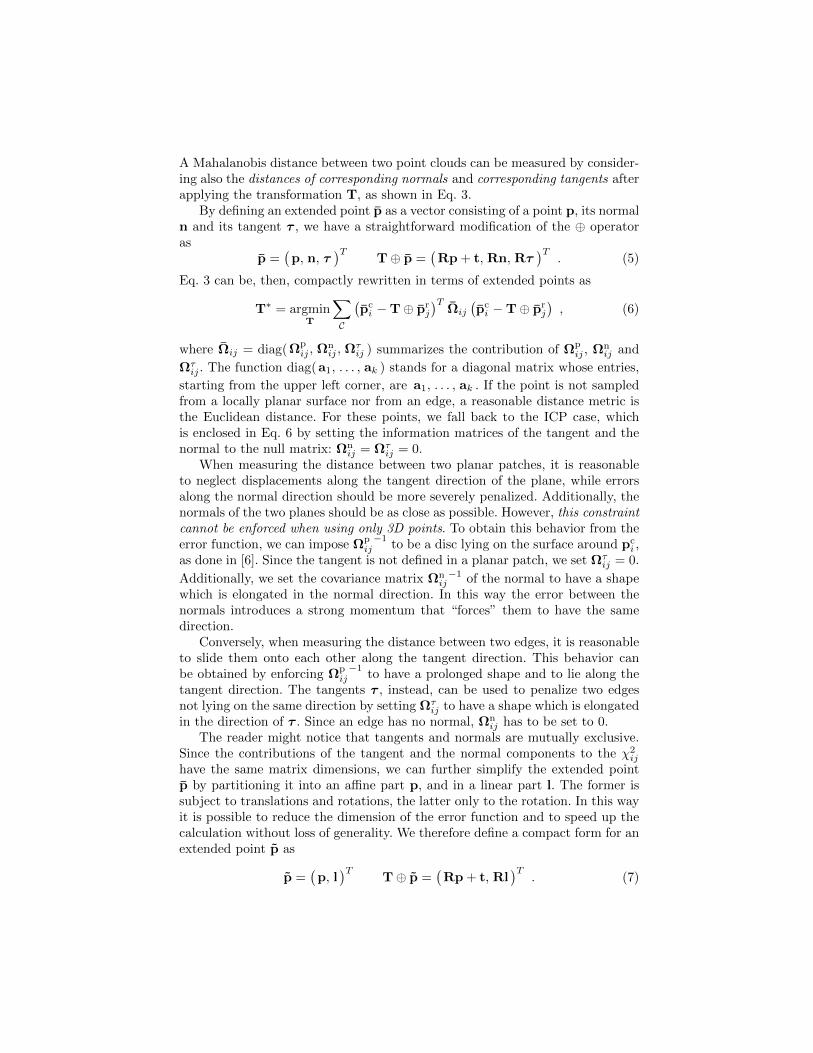
A Mahalanobis distance between two point clouds can be measured by consider-ing also the distances of corresponding normals and corresponding tangents afterapplying the transformation T, as shown in Eq. 3.

By defining an extended point p as a vector consisting of a point p, its normaln and its tangent τ , we have a straightforward modification of the ⊕ operatoras

p =(p, n, τ

)TT⊕ p =

(Rp + t, Rn, Rτ

)T. (5)

Eq. 3 can be, then, compactly rewritten in terms of extended points as

T∗ = argminT

∑C

(pci −T⊕ pr

j

)TΩij

(pci −T⊕ pr

j

), (6)

where Ωij = diag(Ωpij , Ω

nij , Ω

τij ) summarizes the contribution of Ωp

ij , Ωnij and

Ωτij . The function diag(a1, . . . , ak ) stands for a diagonal matrix whose entries,

starting from the upper left corner, are a1, . . . , ak . If the point is not sampledfrom a locally planar surface nor from an edge, a reasonable distance metric isthe Euclidean distance. For these points, we fall back to the ICP case, whichis enclosed in Eq. 6 by setting the information matrices of the tangent and thenormal to the null matrix: Ωn

ij = Ωτij = 0.

When measuring the distance between two planar patches, it is reasonableto neglect displacements along the tangent direction of the plane, while errorsalong the normal direction should be more severely penalized. Additionally, thenormals of the two planes should be as close as possible. However, this constraintcannot be enforced when using only 3D points. To obtain this behavior from theerror function, we can impose Ωp

ij−1

to be a disc lying on the surface around pci ,

as done in [6]. Since the tangent is not defined in a planar patch, we set Ωτij = 0.

Additionally, we set the covariance matrix Ωnij−1 of the normal to have a shape

which is elongated in the normal direction. In this way the error between thenormals introduces a strong momentum that “forces” them to have the samedirection.

Conversely, when measuring the distance between two edges, it is reasonableto slide them onto each other along the tangent direction. This behavior canbe obtained by enforcing Ωp

ij−1

to have a prolonged shape and to lie along thetangent direction. The tangents τ , instead, can be used to penalize two edgesnot lying on the same direction by setting Ωτ

ij to have a shape which is elongatedin the direction of τ . Since an edge has no normal, Ωn

ij has to be set to 0.The reader might notice that tangents and normals are mutually exclusive.

Since the contributions of the tangent and the normal components to the χ2ij

have the same matrix dimensions, we can further simplify the extended pointp by partitioning it into an affine part p, and in a linear part l. The former issubject to translations and rotations, the latter only to the rotation. In this wayit is possible to reduce the dimension of the error function and to speed up thecalculation without loss of generality. We therefore define a compact form for anextended point p as

p =(p, l

)TT⊕ p =

(Rp + t, Rl

)T. (7)

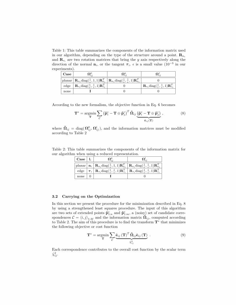
Table 1: This table summarizes the components of the information matrix usedin our algorithm, depending on the type of the structure around a point. Rni

and Rτi are two rotation matrices that bring the y axis respectively along thedirection of the normal ni, or the tangent τ i. ε is a small value (10−3 in ourexperiments).

Case Ωpij Ωn

ij Ωτij

planar Rnidiag( 1ε, 1, 1)RT

niRnidiag( 1

ε, 1ε, 1)RT

ni0

edge Rτidiag( 1ε, 1ε, 1)RT

τi 0 Rτidiag( 1ε, 1ε, 1)RT

τi

none I 0 0

According to the new formalism, the objective function in Eq. 6 becomes

T∗ = argminT

∑C

(pci −T⊕ pr

j

)TΩij

(pci −T⊕ pr

j

)︸ ︷︷ ︸eij(T)

, (8)

where Ωij = diag(Ωpij , Ω

lij ), and the information matrices must be modified

according to Table 2

Table 2: This table summarizes the components of the information matrix forour algorithm when using a reduced representation.

Case li Ωpij Ωl

ij

planar ni Rnidiag( 1ε, 1, 1)RT

niRnidiag( 1

ε, 1ε, 1)RT

ni

edge τ i Rτidiag( 1ε, 1ε, 1)RT

τi Rτidiag( 1ε, 1ε, 1)RT

τi

none 0 I 0

3.2 Carrying on the Optimization

In this section we present the procedure for the minimization described in Eq. 8by using a strengthened least squares procedure. The input of this algorithmare two sets of extended points pc

1:n and pc1:m, a (noisy) set of candidate corre-

spondences C = 〈i, j〉1:M and the information matrix Ωij , computed accordingto Table 2. The aim of this procedure is to find the transform T∗ that minimizesthe following objective or cost function

T∗ = argminT

∑C

eij (T)T

Ωij eij (T)︸ ︷︷ ︸χ2ij

. (9)

Each correspondence contributes to the overall cost function by the scalar termχ2ij .

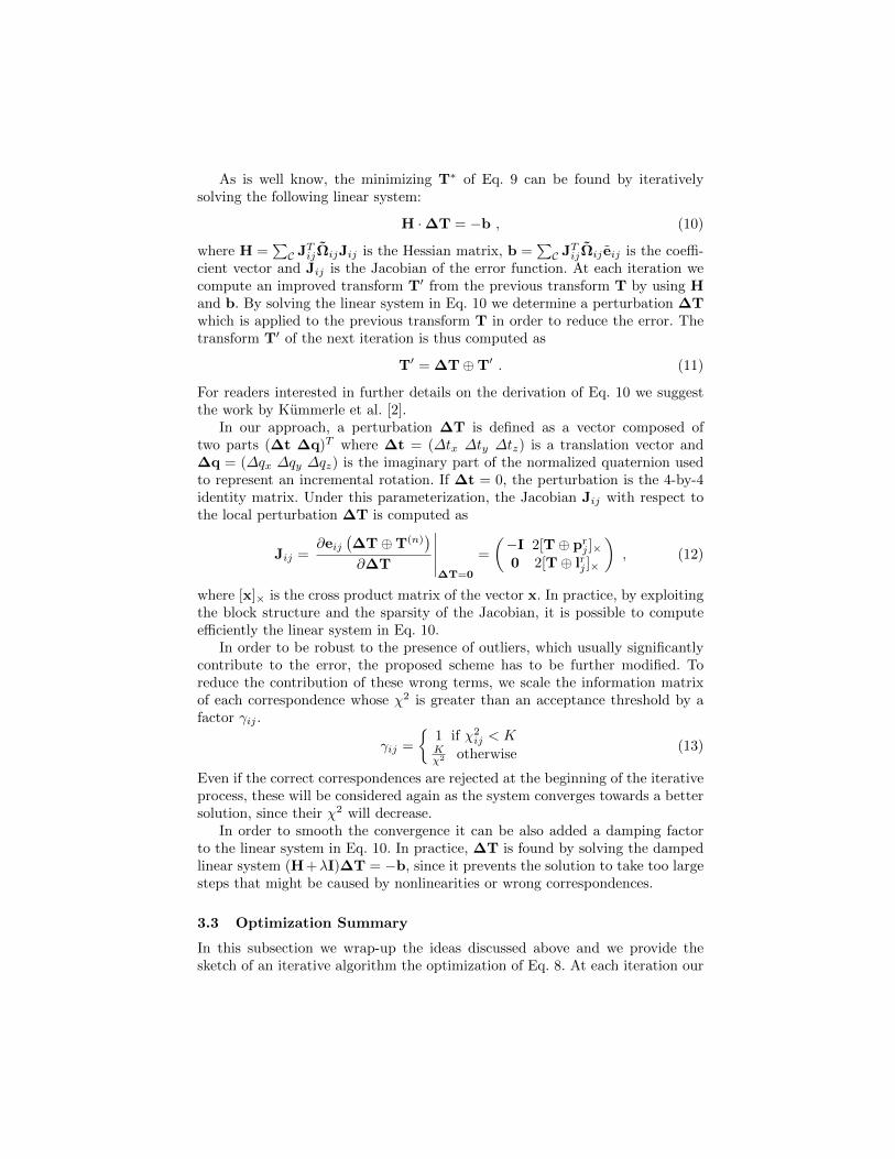
As is well know, the minimizing T∗ of Eq. 9 can be found by iterativelysolving the following linear system:

H ·∆T = −b , (10)

where H =∑C JTijΩijJij is the Hessian matrix, b =

∑C JTijΩij eij is the coeffi-

cient vector and Jij is the Jacobian of the error function. At each iteration wecompute an improved transform T′ from the previous transform T by using Hand b. By solving the linear system in Eq. 10 we determine a perturbation ∆Twhich is applied to the previous transform T in order to reduce the error. Thetransform T′ of the next iteration is thus computed as

T′ = ∆T⊕T′ . (11)

For readers interested in further details on the derivation of Eq. 10 we suggestthe work by Kummerle et al. [2].

In our approach, a perturbation ∆T is defined as a vector composed oftwo parts (∆t ∆q)T where ∆t = (∆tx ∆ty ∆tz) is a translation vector and∆q = (∆qx ∆qy ∆qz) is the imaginary part of the normalized quaternion usedto represent an incremental rotation. If ∆t = 0, the perturbation is the 4-by-4identity matrix. Under this parameterization, the Jacobian Jij with respect tothe local perturbation ∆T is computed as

Jij =∂eij

(∆T⊕T(n)

)∂∆T

∣∣∣∣∣∆T=0

=

(−I 2[T⊕ pr

j ]×0 2[T⊕ lrj ]×

), (12)

where [x]× is the cross product matrix of the vector x. In practice, by exploitingthe block structure and the sparsity of the Jacobian, it is possible to computeefficiently the linear system in Eq. 10.

In order to be robust to the presence of outliers, which usually significantlycontribute to the error, the proposed scheme has to be further modified. Toreduce the contribution of these wrong terms, we scale the information matrixof each correspondence whose χ2 is greater than an acceptance threshold by afactor γij .

γij =

1 if χ2

ij < KKχ2 otherwise

(13)

Even if the correct correspondences are rejected at the beginning of the iterativeprocess, these will be considered again as the system converges towards a bettersolution, since their χ2 will decrease.

In order to smooth the convergence it can be also added a damping factorto the linear system in Eq. 10. In practice, ∆T is found by solving the dampedlinear system (H+λI)∆T = −b, since it prevents the solution to take too largesteps that might be caused by nonlinearities or wrong correspondences.

3.3 Optimization Summary

In this subsection we wrap-up the ideas discussed above and we provide thesketch of an iterative algorithm the optimization of Eq. 8. At each iteration our

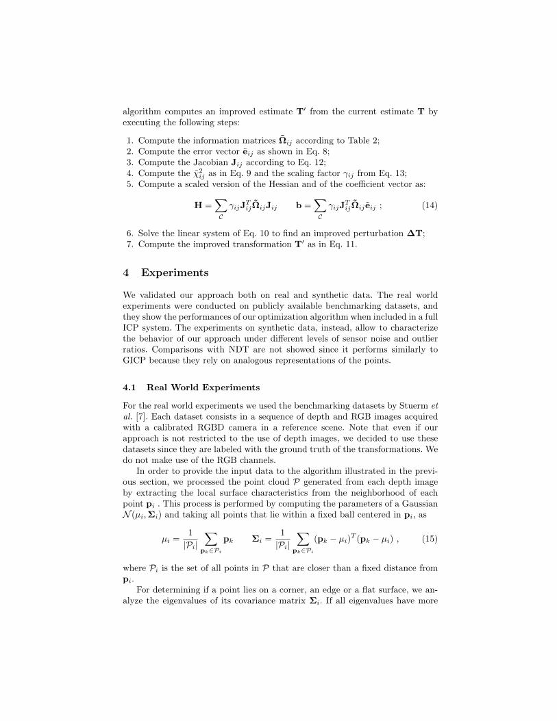
algorithm computes an improved estimate T′ from the current estimate T byexecuting the following steps:

1. Compute the information matrices Ωij according to Table 2;2. Compute the error vector eij as shown in Eq. 8;3. Compute the Jacobian Jij according to Eq. 12;4. Compute the χ2

ij as in Eq. 9 and the scaling factor γij from Eq. 13;5. Compute a scaled version of the Hessian and of the coefficient vector as:

H =∑CγijJ

TijΩijJij b =

∑CγijJ

TijΩij eij ; (14)

6. Solve the linear system of Eq. 10 to find an improved perturbation ∆T;7. Compute the improved transformation T′ as in Eq. 11.

4 Experiments

We validated our approach both on real and synthetic data. The real worldexperiments were conducted on publicly available benchmarking datasets, andthey show the performances of our optimization algorithm when included in a fullICP system. The experiments on synthetic data, instead, allow to characterizethe behavior of our approach under different levels of sensor noise and outlierratios. Comparisons with NDT are not showed since it performs similarly toGICP because they rely on analogous representations of the points.

4.1 Real World Experiments

For the real world experiments we used the benchmarking datasets by Stuerm etal. [7]. Each dataset consists in a sequence of depth and RGB images acquiredwith a calibrated RGBD camera in a reference scene. Note that even if ourapproach is not restricted to the use of depth images, we decided to use thesedatasets since they are labeled with the ground truth of the transformations. Wedo not make use of the RGB channels.

In order to provide the input data to the algorithm illustrated in the previ-ous section, we processed the point cloud P generated from each depth imageby extracting the local surface characteristics from the neighborhood of eachpoint pi . This process is performed by computing the parameters of a GaussianN (µi,Σi) and taking all points that lie within a fixed ball centered in pi, as

µi =1

|Pi|∑

pk∈Pi

pk Σi =1

|Pi|∑

pk∈Pi

(pk − µi)T (pk − µi) , (15)

where Pi is the set of all points in P that are closer than a fixed distance frompi.

For determining if a point lies on a corner, an edge or a flat surface, we an-alyze the eigenvalues of its covariance matrix Σi. If all eigenvalues have more

or less the same magnitude, we assume the point is on a corner. If one of theeigenvalues is smaller with respect to the other two, we assume the point lieson an edge. Finally, if one of the eigenvalues is smaller of some order of magni-tude with respect to the others then we assume the point is on a planar patch.This discrimination is necessary to compute the correct information matrices,according to Table 2.

Given two clouds to be aligned, we search the correspondences using a lineof sight criterion over the depth images, we reject the correspondences whosenormals are too different and we execute one iteration of optimization. Noticethat ICP and GICP are special cases that can be captured by our algorithm justby modifying the way in which the information matrices are computed. To focusour analysis on the objective function we left all parts of the system unchanged,including the correspondence selection. This represents an advantage for plainICP, since normally it does not rely on the normals in order to reject wrongassociations.

For each dataset, we incrementally aligned one frame to the previous one.For each iteration of the alignment, we compared the difference between thecurrent solution and the ground truth. Each attempted alignment produced aplot which shows the evolution of the rotational and translational error. Forcompactness, we provide in this paper only the average error plots obtained byaveraging all errors of a run1. The reader who is interested in the individual plotsof each alignment, can find them at http://www.dis.uniroma1.it/~serafin/publications/icp-augmented-measurements.

In order to measure the robustness of the alignments to wrong initial guesseswe performed several runs of the experiments by considering a frame each N .Table 3 shows the average evolution of the rotational and the translational erroron three different datasets and at different frame skips.

The plotted results point out that our novel objective function in generalperforms better than the other approaches, in particular in terms of convergencespeed. This is true especially for the rotational part of the error since it is in-fluenced directly by the normals. Also in the case where no frame was skipped(first column of Table 3), GICP required twice the number of iterations to con-verge to the results of our approach. Moreover, ICP and GICP showed much lessrobustness to frame skipping (second and third column of Table 3).

4.2 Experiments on Synthetic Data

We conducted experiments on synthetic data in order to assess the effects ofthe inliers and of the sensor error on our optimization function. To this end wegenerated a scene consisting of about 300k 3D points with normals and tangents.Then, we computed the correct correspondences and ideal measurements and wecorrupted them. This process has been performed by injecting a variable fractionof random outliers and perturbing the measurements by adding Gaussian noise

1 With run we denote all the alignment over a single dataset with a certain frame skiprate.

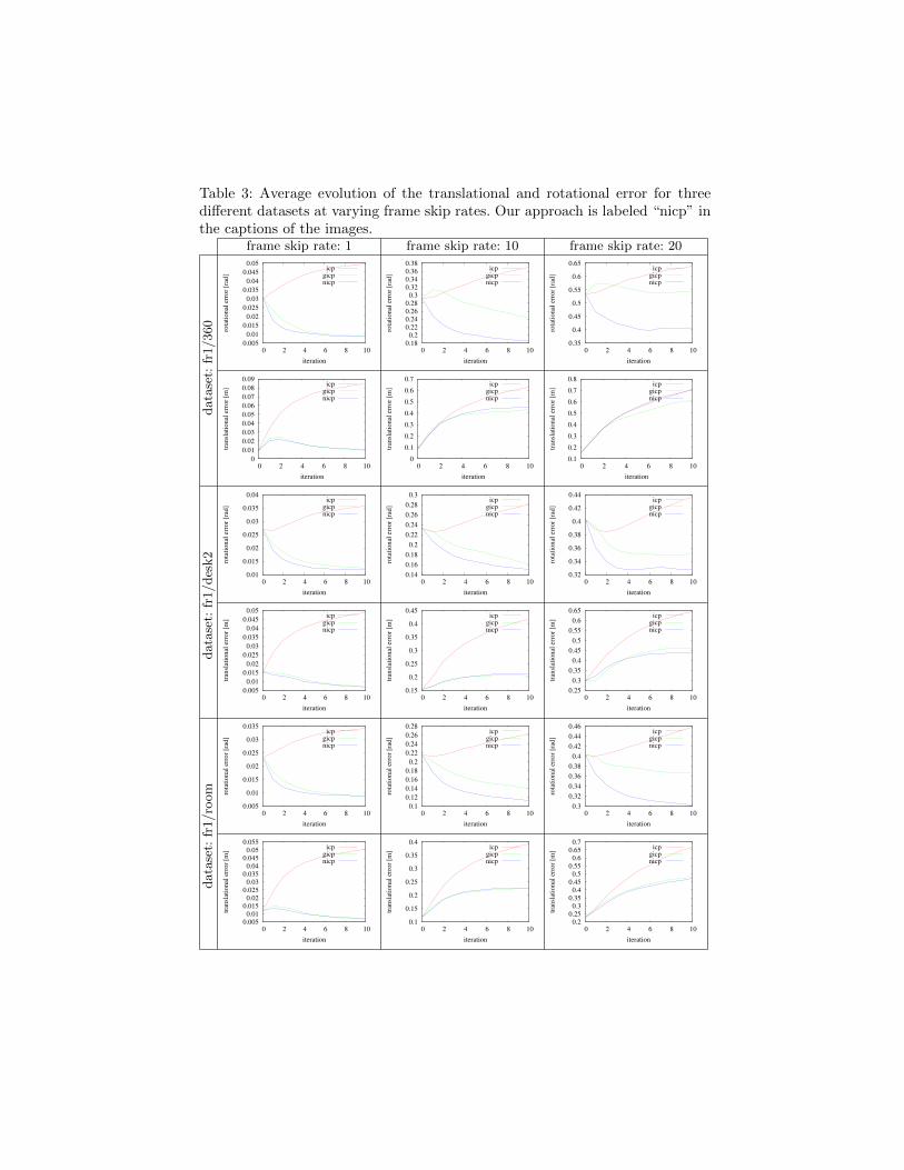
Table 3: Average evolution of the translational and rotational error for threedifferent datasets at varying frame skip rates. Our approach is labeled “nicp” inthe captions of the images.

frame skip rate: 1 frame skip rate: 10 frame skip rate: 20

data

set:

fr1/360

0.005

0.01

0.015

0.02

0.025

0.03

0.035

0.04

0.045

0.05

0 2 4 6 8 10

rota

tio

nal

err

or

[rad

]

iteration

icpgicpnicp

0.18

0.2

0.22

0.24

0.26

0.28

0.3

0.32

0.34

0.36

0.38

0 2 4 6 8 10

rota

tio

nal

err

or

[rad

]

iteration

icpgicpnicp

0.35

0.4

0.45

0.5

0.55

0.6

0.65

0 2 4 6 8 10

rota

tio

nal

err

or

[rad

]

iteration

icpgicpnicp

0

0.01

0.02

0.03

0.04

0.05

0.06

0.07

0.08

0.09

0 2 4 6 8 10

tran

slat

ion

al e

rro

r [m

]

iteration

icpgicpnicp

0

0.1

0.2

0.3

0.4

0.5

0.6

0.7

0 2 4 6 8 10

tran

slat

ion

al e

rro

r [m

]

iteration

icpgicpnicp

0.1

0.2

0.3

0.4

0.5

0.6

0.7

0.8

0 2 4 6 8 10

tran

slat

ion

al e

rro

r [m

]

iteration

icpgicpnicp

data

set:

fr1/des

k2

0.01

0.015

0.02

0.025

0.03

0.035

0.04

0 2 4 6 8 10

rota

tio

nal

err

or

[rad

]

iteration

icpgicpnicp

0.14

0.16

0.18

0.2

0.22

0.24

0.26

0.28

0.3

0 2 4 6 8 10

rota

tio

nal

err

or

[rad

]

iteration

icpgicpnicp

0.32

0.34

0.36

0.38

0.4

0.42

0.44

0 2 4 6 8 10

rota

tio

nal

err

or

[rad

]

iteration

icpgicpnicp

0.005

0.01

0.015

0.02

0.025

0.03

0.035

0.04

0.045

0.05

0 2 4 6 8 10

tran

slat

ion

al e

rro

r [m

]

iteration

icpgicpnicp

0.15

0.2

0.25

0.3

0.35

0.4

0.45

0 2 4 6 8 10

tran

slat

ion

al e

rro

r [m

]

iteration

icpgicpnicp

0.25

0.3

0.35

0.4

0.45

0.5

0.55

0.6

0.65

0 2 4 6 8 10

tran

slat

ion

al e

rro

r [m

]

iteration

icpgicpnicp

data

set:

fr1/ro

om

0.005

0.01

0.015

0.02

0.025

0.03

0.035

0 2 4 6 8 10

rota

tio

nal

err

or

[rad

]

iteration

icpgicpnicp

0.1

0.12

0.14

0.16

0.18

0.2

0.22

0.24

0.26

0.28

0 2 4 6 8 10

rota

tio

nal

err

or

[rad

]

iteration

icpgicpnicp

0.3

0.32

0.34

0.36

0.38

0.4

0.42

0.44

0.46

0 2 4 6 8 10

rota

tio

nal

err

or

[rad

]

iteration

icpgicpnicp

0.005

0.01

0.015

0.02

0.025

0.03

0.035

0.04

0.045

0.05

0.055

0 2 4 6 8 10

tran

slat

ion

al e

rro

r [m

]

iteration

icpgicpnicp

0.1

0.15

0.2

0.25

0.3

0.35

0.4

0 2 4 6 8 10

tran

slat

ion

al e

rro

r [m

]

iteration

icpgicpnicp

0.2

0.25

0.3

0.35

0.4

0.45

0.5

0.55

0.6

0.65

0.7

0 2 4 6 8 10

tran

slat

ion

al e

rro

r [m

]

iteration

icpgicpnicp

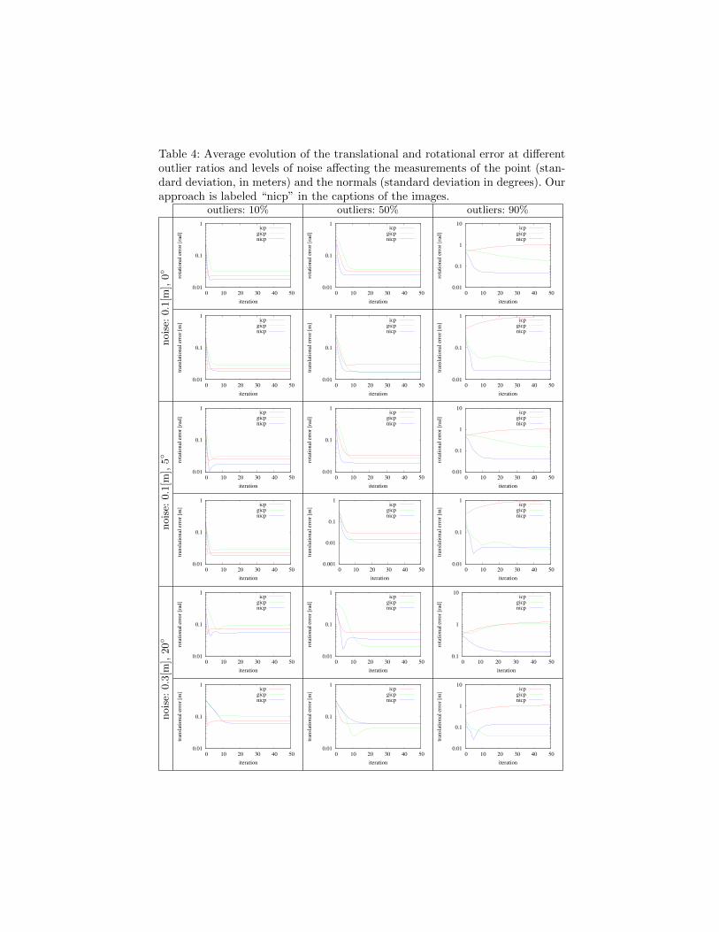
Table 4: Average evolution of the translational and rotational error at differentoutlier ratios and levels of noise affecting the measurements of the point (stan-dard deviation, in meters) and the normals (standard deviation in degrees). Ourapproach is labeled “nicp” in the captions of the images.

outliers: 10% outliers: 50% outliers: 90%

nois

e:0.1

[m],

0

0.01

0.1

1

0 10 20 30 40 50

rota

tio

nal

err

or

[rad

]

iteration

icpgicpnicp

0.01

0.1

1

0 10 20 30 40 50

rota

tio

nal

err

or

[rad

]

iteration

icpgicpnicp

0.01

0.1

1

10

0 10 20 30 40 50

rota

tio

nal

err

or

[rad

]

iteration

icpgicpnicp

0.01

0.1

1

0 10 20 30 40 50

tran

slat

ion

al e

rro

r [m

]

iteration

icpgicpnicp

0.01

0.1

1

0 10 20 30 40 50

tran

slat

ion

al e

rro

r [m

]

iteration

icpgicpnicp

0.01

0.1

1

0 10 20 30 40 50

tran

slat

ion

al e

rro

r [m

]

iteration

icpgicpnicp

nois

e:0.1

[m],

5

0.01

0.1

1

0 10 20 30 40 50

rota

tio

nal

err

or

[rad

]

iteration

icpgicpnicp

0.01

0.1

1

0 10 20 30 40 50

rota

tio

nal

err

or

[rad

]

iteration

icpgicpnicp

0.01

0.1

1

10

0 10 20 30 40 50

rota

tio

nal

err

or

[rad

]

iteration

icpgicpnicp

0.01

0.1

1

0 10 20 30 40 50

tran

slat

ion

al e

rro

r [m

]

iteration

icpgicpnicp

0.001

0.01

0.1

1

0 10 20 30 40 50

tran

slat

ion

al e

rro

r [m

]

iteration

icpgicpnicp

0.01

0.1

1

0 10 20 30 40 50

tran

slat

ion

al e

rro

r [m

]

iteration

icpgicpnicp

nois

e:0.3

[m],

20

0.01

0.1

1

0 10 20 30 40 50

rota

tio

nal

err

or

[rad

]

iteration

icpgicpnicp

0.01

0.1

1

0 10 20 30 40 50

rota

tio

nal

err

or

[rad

]

iteration

icpgicpnicp

0.1

1

10

0 10 20 30 40 50

rota

tio

nal

err

or

[rad

]

iteration

icpgicpnicp

0.01

0.1

1

0 10 20 30 40 50

tran

slat

ion

al e

rro

r [m

]

iteration

icpgicpnicp

0.01

0.1

1

0 10 20 30 40 50

tran

slat

ion

al e

rro

r [m

]

iteration

icpgicpnicp

0.01

0.1

1

10

0 10 20 30 40 50

tran

slat

ion

al e

rro

r [m

]

iteration

icpgicpnicp

to the points and normal estimates. For each setting we ran our approach, ICPand GICP, and we plotted the evolution of the translational and rotational error.The results are shown in Table 4.

Overall the experiments on synthetic data reflect the behavior of the realworld ones. Shortly, using additional information in the error function makesthe approach more robust and accelerates the convergence. This is particularlytrue at high rates of outliers and sensor noise. Not surprisingly, instead, noise inthe normals lowers the performances. In the unrealistic scenario in which everynormal is affected by a 20 error at 90% of outliers the translational estimatebecomes less accurate than GICP, but it still converges to a reasonable solution.

5 Conclusions

In this paper we proposed a novel optimization function to register point cloudsusing an ICP based algorithm that takes into account an augmented measure-ment vector. Statistical comparative experiments on real and synthetic datashow that our approach performs better than other state of the art methodsboth in terms of convergence speed and robustness. As expected, the normalsand the tangents of the surfaces showed an improvement in particular in the ro-tational part of the error, while keeping the translational one similar to the otherapproaches. A further enhancement could be obtained by finding an additionalmeasurement, related to the translation, to be considered in the minimizationof the cost function.

Acknowledgments. This work has partly been supported by the EuropeanCommission under FP7-600890-ROVINA.

References

1. Besl, P.J., McKay, N.D.: A method for registration of 3-D shapes. IEEE Transactionson Pattern Analysis and Machine Intelligence (1992)

2. Grisetti, G., Kummerle, R., Stachniss, C., Burgard, W.: A tutorial on graph-basedslam. Intelligent Transportation Systems Magazine, IEEE 2(4), 31–43 (2010)

3. Horn, B.K., Hilden, H.M., Negahdaripour, S.: Closed-form solution of absolute ori-entation using orthonormal matrices. Journal of the Optical Society of America(1988)

4. Magnusson, M., Duckett, T., Lilienthal, A.J.: Scan registration for autonomous min-ing vehicles using 3d-ndt. Journal on Field Robotics (2007)

5. Pomerleau, F., Colas, F., Siegwart, R., Magnenat, S.: Comparing icp variants onreal-world data sets. Autonomous Robots (2013)

6. Segal, A.V., Haehnel, D., Thrun, S.: Generalized-ICP. In: Proc. of Robotics: Scienceand Systems (RSS) (2009)

7. Sturm, J., Engelhard, N., Endres, F., Burgard, W., Cremers, D.: A benchmark forthe evaluation of rgb-d slam systems. In: Proc. of the IEEE/RSJ Int. Conf. onIntelligent Robots and Systems (IROS) (2012)