Variational convergence of bivariate functions: lopsided convergence

Math. Program., Ser. BDOI 10.1007/s10107-007-0122-8

FULL LENGTH PAPER

Variational convergence of bivariate functions: lopsidedconvergence

Alejandro Jofré · Roger J.-B. Wets

Received: 11 September 2005 / Accepted: 3 April 2006© Springer-Verlag 2007

Abstract We explore convergence notions for bivariate functions that yieldconvergence and stability results for their maxinf (or minsup) points. This lays thefoundations for the study of the stability of solutions to variational inequalities, thesolutions of inclusions, of Nash equilibrium points of non-cooperative games andWalras economic equilibrium points, of fixed points, of solutions to inclusions, theprimal and dual solutions of convex optimization problems and of zero-sum games.These applications will be dealt with in a couple of accompanying papers.

Keywords Lopsided convergence · Maxinf-points · Ky Fan functions · Variationalinequalities · Epi-convergence

Mathematics Subject Classification (2000) 65K10 · 90C31 · 91A10 · 47J20 ·47J30 · 49J45

Dedicated to A. Auslender in recognition of his valuable contributions to Mathematical Programming:foundations and numerical procedures.

Research supported in part by grants of the National Science Foundation and Fondap-MatematicasAplicadas, Universidad de Chile.

A. JofréCMM and Ingeniería Matemática, Universidad de Chile, Santiago, Chilee-mail: [email protected]

R.J.-B. Wets (B)Department of Mathematics, University of California, Davis, USAe-mail: [email protected]

123

A. Jofré, R. J. -B. Wets

1 Variational convergence of bivariate functions

A fundamental component of ‘Variational Analysis’ is the analysis of the propertiesof bivariate functions. For example: the analysis of the Lagrangians associated withan optimization problem, of the Hamiltonians associated with Calculus of Variationsand Optimal Control problems, the reward functions associated with cooperative ornon-cooperative games, and so on. In a series of articles, we deal with the stabilityof the solutions of a wide collection of problems that can be re-cast as finding themaxinf-points of such bivariate functions.

So, more explicitly: given a bivariate function F : C × D → R, we are interestedin finding a point, say x ∈ C , that maximizes with respect to the first variable x ,the infimum of F , inf y∈D F(·, y), with respect to the second variable y. We refer tosuch a point x as a maxinf-point. In some particular situations, for example when thebivariate function is concave–convex, such a point can be a saddle point, but in manyother situation its just a maxinf-point, or a minsup-point when minimizing with respectto the first variable the supremum of F with respect to the second variable. To study thestability, and the existence, of such points, and the sensitivity of their associated values,one is lead to introduce and analyze convergence notion(s) for bivariate functions thatin turn will guarantee the convergence either of their saddle points or of just theirmaxinf-points.

This paper is devoted to the foundations. Two accompanying papers deal with themotivating examples [10,11]: variational inequalities, fixed points, Nash equilibriumpoints of non-cooperative games, equilibrium points of zero-sum games, etc. We makea distinction between the situations when the bivariate function is generated from asingle-valued mapping [11] or when the mapping can also be set-valued [10].

The major tool is the notion of lopsided convergence, that was introduced in [2], butis modified here so that a wider class of applications can be handled. The major adjust-ment is that bivariate functions are no longer as in [2], defined on all of R

n × Rm with

values in the extended reals, but are now only finite-valued on a specific product C × Dwith C, D subsets of R

n and Rm . Dealing with ‘general’ bivariate functions defined

on the full product space was in keeping with the elegant work of Rockafellar [13]on duality relations for convex–concave bivariate functions and the subsequent work[3] on the epi/hypo-convergence of saddle functions. However, our present analysisactually shows that notwithstanding its esthetic allurement one should not cast bivari-ate functions, even in the convex–concave case, in the general extended-real valuedframework. In some way, this is in contradiction with the univariate case where theextension, by allowing for the values ±∞, of functions defined on a (constrained) setto all of R

n has been so effectively exploited to derive a ‘unified’ convergence anddifferentiation theory [5,14]. We shall show that some of this can be recovered, but onemust first make a clear distinction between max-inf problems and min-sup ones, andonly then one can generate the appropriate extensions; after all, also in the univariatecase one makes a clear distinction when extending a function in a minimization settingor a maximization setting.

In order to be consistent in our presentation, and to set up the results requiredlater on, we begin by a presentation of the theory of epi-convergence for real-valuedunivariate functions that are only defined on a subset of R

n . No ‘new’ results are

123

Variational convergence of bivariate functions

actually derived although a revised formulation is required. We make the connectionwith the standard approach, i.e., when these (univariate) functions are extended real-valued. We then turn to lopsided convergence and point out the shortcomings of an‘extended real-valued’ approach. Finally, we exploit our convergence result to obtaina extension of Ky Fan inequality [7] to situations when the domain of definition of thebivariate function is not necessarily compact.

2 Epi-convergence

One can always represent an optimization problem, involving constraints or not, asone of minimizing an extended real-valued function. In the case of a constrained-minimization problem, simply redefine the objective as taking on the value ∞ out-side the feasible region, the set determined by the constraints. In this framework, thecanonical problem can be formulated as one of minimizing on all of R

n an extendedreal-valued function f : R

n → R. Approximation issues can consequently be stud-ied in terms of the convergence of such functions. This has lead to the notion ofepi-convergence1 that plays a key role in ‘Variational Analysis’ [1,5,14]; when deal-ing with a maximization problem, it is hypo-convergence, the convergence of thehypographs, that is the appropriate convergence notion.

Henceforth, we restrict our development to the ‘minimization setting’ but, at theend of this section, we translate results and observations to the ‘maximization’ case.

As already indicated, in Variational Analysis, one usually deals with

fcn(Rn) = {f : R

n → R}

the space of extended real-valued functions that are defined on all of Rn , even allowing

for the possibility that they are nowhere finite-valued. Definitions, properties, limits,etc., generally do not refer to the domain on which they are finite. For reasons that willbecome clearer when we deal with the convergence of bivariate functions, we need todepart from this simple, and very convenient, paradigm. Our focus will be on

f v-fcn(Rn) = {f : D → R

∣∣ for some ∅ �= D ⊂ R

n},

the class of all finite-valued functions with non-empty domain D ⊂ Rn . It must be

understood that in this notation, Rn does not refer to the domain of definition, but to

the underlying space that contains the domains on which the functions are defined.The epigraph of a function f is always the set of all points in R

n+1 that lie onor above the graph of f , irrespective of f belonging to f v-fcn(Rn) or fcn(Rn). Iff : D → R belongs to f v-fcn(Rn), then

epi f = {(x, α) ∈ D × R

∣∣ α ≥ f (x)

} ⊂ Rn+1,

1 For extensive references and a survey of the field one can consult [1,5], and in particular, the Commentarysection that concludes [14, Chap. 7].

123


and if f belongs to fcn(Rn) then

epi f = {(x, α) ∈ R

n+1∣∣α ≥ f (x)

}.

A function f is lsc (=lower semicontinuous) if its epigraph is closed as a subset ofR

n+1, i.e., epi f = cl(epi f ) with cl denoting closure [14, Theorem 1.6].2

So, when f ∈ f v-fcn(Rn), lsc implies3 that for all xν ∈ D → x :

– if x ∈ D: liminfν f (xν) ≥ f (x), and– if x ∈ cl D \ D: f (xν) → ∞.

In our ‘minimization’ framework: cl f denotes the function whose epigraph is theclosure relative to R

n+1 of the epigraph of f , i.e., the lsc-regularization of f . Itspossible that when f ∈ f v-fcn, cl f might be defined on a set thats strictly larger thanD but always contained in cl D.

Lets now turn to convergence issues. Recall that set-convergence, in the Painlevé–Kuratowski sense [14, Sect. 4.B], is defined as follows: Cν → C ⊂ R

n if

– (a-set) all cluster points of a sequence{

xν ∈ Cν}ν∈IN belong to C ,

– (b-set) for each x ∈ C , one can find a sequence xν ∈ Cν → x .

When just condition (a-set) holds, then C is then the outer limit of the sequence{Cν

}ν∈IN , and when its just (b-set) that holds, then C is the inner limit [14, Chap. 4,

Sect. 2]. Note, that whenever C is the limit, the outer- or the inner-limit, its closed[14, Proposition 4.4] and that C = ∅ if and only if the sequence Cν eventually ‘es-capes’ from any bounded set [14, Corollary 4.11]. Moreover, if the sequence

{Cν

}ν∈IN

consists of convex sets, its inner limit, and its limit if it exists, are also convex [14,Proposition 4.15].

Definition 1 (epi-convergence) A sequence of functions{

f ν, ν ∈ IN}, whose

domains lie in Rn , epi-converges to a function f when epi f ν → epi f as subsets

of Rn+1; again irrespective of f belonging to f v-fcn(Rn) or fcn(Rn). One then writes

f ν →e f .

Figure 1 provides an example of two functions f and f ν that are close to eachother in terms of the distance between their epigraphs—i.e., the distance between thelocation of the two jumps—but are pretty far from each other pointwise or with respectto the �∞-norm,—i.e., the size of the jumps.

Let { f ν}ν∈IN be a sequence of functions with domains in Rn . When,

– epi f is the outer limit of {epi f ν}ν∈IN , one refers to f as the lower epi-limit of thefunctions f ν ,

– epi f is the inner limit of the epi f ν , one refers to f as the upper epi-limit of thefunctions f ν .

Of course, f is the epi-limit of the sequence if its both the lower and upper epi-limit.

2 Throughout its implicitly assumed that Rn is equipped with its usual Euclidiean topology.

3 Indeed, if liminfν f (xν) < ∞, then for some subsequence {νk }, f (xνk ) → α ∈ R and because epi f isclosed, it implies that (x, α) ∈ epi f which would place x in the domain of f , contradicting x /∈ D.

123


x

f

f

Fig. 1 f and f ν epigraphically close to each other

Proposition 1 (properties of epi-limits) Let { f ν}ν∈IN be a sequence of functions withdomains in R

n. Then, the lower and upper epi-limits and the epi-limit, if it exists, areall lsc. Moreover, if the functions f ν are convex, so is the upper epi-limit, and theepi-limit, if it exists.

Proof Follows immediately from the properties of set-limits. �The last proposition implies in particular that the family of lsc functions is closed

under epi-convergence.The definition of epi-convergence for families of functions in fcn(Rn) is the usual

one [14, Chap. 7, Sect. B] with all the implications concerning the convergence ofthe minimizers and infimal values [14, Chap. 7, Sect. E]. But, in a certain sense, thedefinition is ‘new’ when the focus is on epi-convergent families in f v-fcn(Rn), andits for this class of functions that we need to know the conditions under which one canclaim convergence of the minimizers and infimums. We chose to make the presentationself-contained, although as will be shown later, one could also embed f v-fcn(Rn) ina subclass of fcn(Rn) and then appeal to the ‘standard’ results, but unfortunately thisrequires that the non-initiated reader plows through a substantial amount of material.

When f is an epi-limit its necessarily a lsc function since its epigraph is the set-limit of a collection of sets in R

n+1. Its epigraph is closed but its domain D is notnecessarily closed. Simply think of the collection of functions f ν = f for all ν withD = (0,∞) and f (x) = 1/x on D. This collection clearly epi-converges to the lscfunction f on D with closed epigraph but not with closed domain.

Lemma 1 (epi-limit value at boundary points). Suppose f : D → R is the epi-limitof a sequence

{f ν : Dν → R

}ν∈IN with all functions in f v-fcn(Rn). Then, for any

sequence xν ∈ Dν → x: liminfν f ν(xν) > −∞.

Proof We proceed by contradiction. Suppose that xν ∈ Dν → x andliminfν f ν(xν) = −∞. By assumption f > −∞ on D, thus the xν cannot convergeto a point in D, i.e., necessarily x /∈ D. If thats the case and since epi f ν → epi f ,the line {x} × R would have to lie in epi f contradicting the assumption that f , theepi-limit of the f ν , belongs to f v-fcn(Rn). �

123


Example 1 [an epi-limit thats not in f v-fcn(Rn)] Consider the sequence of functions{f ν : [0,∞) → R

}ν∈IN with

f ν(x) =

⎧⎪⎨

⎪⎩

−ν2x if 0 ≤ x ≤ ν−1,

ν2x − 2ν if ν−1 ≤ x ≤ 2ν−1,

0 for x ≥ 2ν−1.

Detail The functions f ν ∈ f v-fcn(R) and for the sequence xν = ν−1, f ν(xν) → −∞and f ν →e f where f : [0,∞) → R with f ≡ 0 on (0,∞) and f (0) = −∞. Thus, thefunctions f ν epi-converge to f as functions in fcn(R), provided they are appropriatelyextended, i.e., taking on the value ∞ on (−∞, 0). But they do not epi-converge to afunction in f v-fcn(R). �

In addition to the ‘geometric’ definition, the next proposition provides an ‘analytic’characterization of epi-converging sequences in f v-fcn(Rn).

Proposition 2 [epi-convergence in f v-fcn(Rn)] Let{

f : D → R, f ν : Dν →R, ν ∈ IN

}be a collection of functions in f v-fcn(Rn). Then, f ν →e f if and only the

following conditions are satisfied:(a) ∀ xν ∈ Dν → x in D, liminfν f ν(xν) ≥ f (x),(a∞) for all xν ∈ Dν → x /∈ D, f ν(xν)↗∞,4

(b) ∀x ∈ D, ∃ xν ∈ Dν → x such that limsupν f ν(xν) ≤ f (x).

Proof If epi f ν → epi f and xν ∈ Dν → x either lim infν f ν(xν) = α < ∞ ornot; Lemma 1 reminds us that α = −∞ is not a possibility. In the first instance,(x, α) is a cluster point of

{(xν, f ν(xν)) ∈ epi f ν

}ν∈IN and thus belongs to epi f ,

i.e., f (x) ≤ α and hence (a) holds; α > −∞ since otherwise f would not be finitevalued on D. If α = ∞ that means that f ν(xν)↗∞ and x cannot belong to D,and thus (a∞) holds. On the other hand, if x ∈ D and thus f (x) is finite, there isa

{(xν, αν) ∈ epi f ν

}ν∈IN such that xν ∈ Dν → x ∈ D and αν → f (x) with

αν ≥ f ν(xν), i.e., lim supν f ν(xν) ≤ f (x), i.e., (b) is also satisfied.Conversely, if (a) and (a∞) hold, and (xν, αν) ∈ epi f ν → (x, α) then either x ∈ D

or not; recall also, that in view of Lemma 1, α cannot be −∞ since we are dealingwith epi-convergence in f v-fcn(Rn). In the latter instance, by (a∞) α = ∞, so we arenot dealing with a converging sequence of points (in Rn+1) and there is no need toconsider this situation any further. When x ∈ D, since then lim infν f ν(xν) ≥ f (x)

and αν ≥ f ν(xν), one has α ≥ f (x) and consequently (x, α) belongs to epi f ;this means that condition (a-set) is satisfied. If (x, α) ∈ epi f , from (b) follows theexistence of a sequence xν ∈ Dν → x such that lim supν f ν(xν) ≤ f (x) ≤ α. Wecan then choose the αν ≥ f ν(xν) so that αν → α that yields (b-set), the secondcondition for the set-convergence of epi f ν → epi f . �Theorem 1 (epi-convergence: basic properties) Consider a sequence

{f ν : Dν →

R, ν ∈ IN } ⊂ f v-fcn(Rn) epi-converging to f : D → R, also in f v-fcn(Rn). Then

4 ↗ means non-decreasing and converging to, i.e., not necessarily monotonically.

123


lim supν→∞

(inf f ν) ≤ inf f.

Moreover, if xk ∈ argminDνk f νk for some subsequence {νk} and xk → x , thenx ∈ argminD f and minDνk f νk → minD f .

If argminD f is a singleton, then every convergent subsequence of minimizers con-verges to argminD f .

Proof Let {xl}∞l=1 be a sequence in D such that f (xl) → inf f . By 2(b), for each lone can find a sequence xν,l ∈ Dν → xl such that lim supν f ν(xν,l) ≤ f (xl). Sincefor all ν, inf f ν ≤ f ν(xν,l), it follows that for all l,

lim supν

(inf f ν) ≤ lim supν

f ν(xν,l) ≤ f (xl),

and one has, lim supν(inf f ν) ≤ inf f since f (xl) → inf f .For the sequence xk ∈ Dνk → x , from the above and 2(a),

inf f ≥ lim supk

f νk (xk) ≥ lim infk

f νk (xk) ≥ f (x),

i.e., x minimizes f on D and f νk (xk) = minDνk f νk → minD f .Finally, since every convergent subsequence of minimizers of the functions f ν

converges to a minimizer of f , it follows that it must converge to the unique minimizerwhen argminD f is a singleton. �

In most of the applications, we shall rely on a somewhat more restrictive notionthan ‘simple’ epi-convergence to guarantee the convergence of the infimums.

Definition 2 (tight epi-convergence) The sequence{ f ν : Dν → R}ν∈IN ⊂ f v-fcn(Rn) epi-converges tightly to f : D → R ∈f v-fcn(Rn), if f ν →e f and for all ε > 0, there exist a compact set Bε and an in-dex νε such that

∀ ν ≥ νε : inf Bε∩Dν f ν ≤ inf Dν f ν + ε.

Theorem 2 (convergence of the infimums). Let { f ν : Dν → R}ν∈IN ⊂ f v-fcn(Rn)

be a sequence of functions that epi-converges to the function f : D → R also inf v-fcn(Rn), with inf D f finite. Then, they epi-converge tightly

(a) if and only if inf Dν f ν → inf D f .(b) if and only if there exists a sequence εν ↘ 0 such that εν-argmin f ν → argmin f .

Proof Lets start with necessity in (a). For given ε > 0, the assumptions and Theorem 1imply

lim infν

( infDν∩Bε

f ν) ≤ lim infν

(infDν

f ν) + ε ≤ lim supν

(infDν

f ν) + ε ≤ infD

f + ε < ∞.

123


If there is a subsequence {νk} such that f (xk) < κ for some xk ∈ Dνk ∩ Bε, it wouldfollow that inf D f < κ . Indeed, since Bε is compact, the sequence {xk} has a clusterpoint, say x , and then conditions (a∞) and (a) of Proposition 2 guarantee f (x) < κ

with x ∈ D, and consequently, also inf D f < κ . Since its assumed that inf D f is finite,it follows that there is no such sequences with κ arbitrarily negative. In other words,excluding possibly a finite number of indexes, the inf Dν∩Bε f ν stay bounded awayfrom −∞ and one can find xν ∈ ε- argminDν∩Bε

f ν . The sequence {xν}ν∈IN admitsa cluster point, say x , that lies in Bε and again by 2(a∞,a), f (x) ≤ liminfν f ν(xν).Hence,

inf D f − ε ≤ f (x) − ε ≤ liminfν f ν(xν) − ε ≤ liminfν(inf Dν f ν).

In combination with our first string of inequalities and the fact that ε > 0 can bechosen arbitrarily small, it follows that indeed inf Dν f ν → inf D f .

Next, we turn to sufficiency in (a). Since inf f ν → inf f ∈ R by assumption, itsenough, given any δ > 0, to exhibit a compact set B such that lim supν

(inf B∩Dν f ν

) ≤inf D f + δ. Choose any point x such that f (x) ≤ inf D f + δ. Because f ν →e f inf v-fcn(Rn), there exists a sequence, 2(a), xν → x such that lim supν f ν(xν) ≤ f (x).Let B be any compact set large enough to contain all the points xν . Then inf B f ν ≤f ν(xν) for all ν, so B has the desired property.

We derive (b) from (a). Let αν = inf f ν → inf f = α that is finite by assump-tion, and consequently for ν large enough, also αν is finite. Since convergence ofthe epigraphs implies the convergence of the level sets [14, Proposition 7.7], one canfind a sequence of αν ↘ α such that levαν f ν → levα f = argmin f . Simply setεν := αν − αν .

For the converse, suppose there is a sequence εν ↘ 0 with εν-argmin f ν → argminf �= ∅. For any x ∈ argmin f one can select xν ∈ εν-argmin f ν with xν → x . Thenbecause f ν →e f , one obtains

inf f = f (x) ≤ lim infν f ν(xν) ≤ lim infν(inf f ν + εν)

≤ lim infν(inf f ν) ≤ limsupν(inf f ν) ≤ inf f,

where the last inequality comes from Theorem 1. �Remark 1 (convergence of domains) Although, epi-convergence essentially impliesconvergence of the level sets [14, Proposition 7.7], it does not follow that it impliesthe convergence of their (effective) domains. Indeed, consider the following sequencef ν : R → R with f ν ≡ ν except for f ν(0) = 0 that epi-converges to δ{0} the indicatorfunction of {0}. We definitely do not have dom f ν = R converging to dom δ{0} = {0}.This vigorously argues against the temptation of involving the convergence of theirdomains in the definition of epi-convergence, even for functions in f v-fcn(Rn).

This concludes the presentation of the results that will be used in the sequel. Asindicated earlier, its also possible to derive these results from those for extended real-valued functions. To do so, one identifies f v-fcn(Rn) with

pr -fcn(Rn) := {f ∈ fcn(Rn)

∣∣ − ∞ < f �≡ ∞}

,

123


the subset of proper functions in fcn(Rn); in a minimization context, a function f issaid to be proper if f > −∞ and f �≡ ∞, in which case, its finite on its (effective)domain

dom f = {x ∈ R

n∣∣ f (x) < ∞}

.

There is an one-to-one correspondence, a bijection5 denoted η, between the elementsof f v-fcn(Rn) and those of pr -fcn(Rn): If f ∈ f v-fcn(Rn), its extension to all ofR

n by setting η f = f on its domain and η f ≡ ∞ on the complement of its domain,uniquely identifies a function in pr -fcn(Rn). And, if f ∈ pr -fcn(Rn), the restrictionof f to dom f , uniquely identifies a function η−1 f in f v-fcn(Rn). Its important toobserve that under this bijection, any function, either in pr -fcn(Rn) or f v-fcn(Rn),and the corresponding one in f v-fcn(Rn) or pr -fcn(Rn), have the same epigraphs!

Since, epi-convergence for sequences in f v-fcn(Rn) or in in fcn(Rn) is alwaysdefined in terms of the convergence of the epigraphs, there is really no need to verifythat the analytic versions (Proposition 2 and [14, Proposition 7.2]) also coincide.However, for completeness sake and to highlight the connections, we go through thedetails of an argument.

Proposition 3 (epi-convergence in f v-fcn(Rn) and fcn(Rn)) Let{f : D → R, f ν : Dν → R, ν ∈ IN

}be a collection of functions in f v-fcn(Rn).

Then, f ν →e f if and only η f ν →e η f where η is the bijection defined above.

Proof Now, η f ν →e η f ([14, Proposition 7.2]) if and only if for all x ∈ Rn :

(aη) liminfν η f ν(xν) ≥ η f (x) for every sequence xν → x ,(bη) limsupν η f ν(xν) ≤ η f (x) for some sequence xν → x .

Since for x /∈ D, η f (x) = ∞, (aη) clearly implies (a) & (a∞). Conversely, if (a) and(a∞) hold, x ∈ D and xν → x , when computing the liminfν η f ν(xν) one can ignoreelements xν /∈ Dν since then η f ν(xν) = ∞. Hence, for x ∈ D, actually (a) implies(aη). If x /∈ D and xν → x , (a∞) and, again, the fact that η f ν(xν) = ∞ when x /∈ Dν ,yield (aη).

If (bη) hold and x ∈ D, then the sequence xν → x must, at least eventually, havexν ∈ Dν since otherwise the limsupν η f ν(xν) would be ∞ whereas f (x) = η f (x) isfinite. Thus, (bη) implies (b). Conversely, (b) certainly yields (bη) if x ∈ D. If x /∈ D,η f (x) = ∞ and so the inequality in (bη) is also trivially satisfied in that case. �

As long as we restrict our attention to pr -fcn(Rn), in view of the precedingobservations, all the basic results, cf. [14, Chap. 7, Sect. E] of the theory of epi-convergence related to the convergence of infimums and minimizers apply equallywell to functions in f v-fcn(Rn) and not just those featured here. In particular, if onetakes into account the bijection between f v-fcn(Rn) and pr -fcn(Rn), then Theorem 1is simply an adaptation of the standard results for epi-converging sequences in fcn(Rn),cf. [14, Proposition 7.30, Theorem 7.31]. Similarly, again by relying on the bijection

5 In fact, this bijection is a homeomorphism when we restrict our attention to lsc functions. The continuityof this correspondence is immediate if both of these function-spaces are equipped with the topology inducedby the convergence of the epigraphs, see below.

123


η to translate the statement of Theorem 2 into an equivalent one for functions η f ν, η fthat belong to fcn(Rn), one comes up with [14, Theorem 7.31] about the convergenceof the infimal values.

Finally, in a maximization setting, one can simply pass from f to − f , or one canrepeat the previous arguments with the following changes in the terminology: min tomax (inf to sup), ∞ to −∞, epi to hypo, ≤ to ≥ (and vice-versa), lim inf to lim sup(and vice-versa), and lsc to usc. The hypograph of f is the set of all points in R

n+1

that lie on or below the graph of f , f is usc (=upper semicontinuous) if its hypographis closed, and its proper, in the maximization framework, if −∞ �≡ f < ∞; inthe maximization setting cl f denotes the function whose hypograph is the closure,relative to R

n+1 of hypo f , its also called its usc regularization.A sequence is said to hypo-converge, written f ν →h f , when − f ν →e − f , or

equivalently if hypo f ν → hypo f , and it hypo-converge tightly if − f ν epi-convergetightly to − f . And consequently, if the sequence hypo-converges tightly to f withsupD f finite, then supDν f ν → supD f .

When hypo f is the inner set-limit of the hypo f ν , then f is the lower hypo-limitof the functions f ν and if its the outer set-limit then its their upper hypo-limit. It thenfollows from Proposition 1 that the lower and upper hypo-limits, and the hypo-limit,if it exists, are all usc. Moreover, if the functions f ν are concave, so is the lowerhypo-limit, and the hypo-limit, if it exists. Hence, one also has that the family of uscfunctions is closed under hypo-convergence.

3 Lopsided convergence

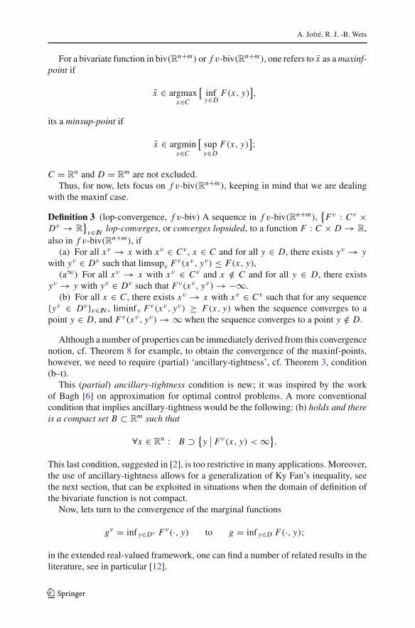
Lopsided convergence for bivariate functions was introduced in [2]; we already reliedon this notion to formalize the convergence of pure exchange economies and to studythe stability of their Walras equilibrium points [9]. Its aimed at the convergence ofmaxinf-points, or minsup-points but not at both; therefore the name lopsided, or lop-convergence. However, our present, more comprehensive, analysis has lead us to adjustthe definition since otherwise some ‘natural’ classes of bivariate functions with domainand values like those depicted in Fig. 2, would essentially be excluded, i.e., could notbe included in (lopsided or) lop-convergent families. And these are precisely the classof functions that needs to be dealt with in many applications. Moreover, like in Sect.2, the main focus will not be on extended real-valued functions but on finite-valuedbivariate functions that are only defined on a product of non-empty sets rather thanon extended real-valued functions defined on the full product space. The motivationfor proceeding in this manner, again, coming from the applications. But this time, itsnot just one possible approach, its in fact mandated by the underlying structure of theclass of bivariates that are of interest in the applications. We shall, however, like in theprevious section, provide the bridge with the ‘extended real-valued’ framework thatwas used in [2].

The definition of lop-convergence is necessarily one-sided. One is either inter-ested in the convergence of maxinf-points or minsup-points but not both. In general,the maxinf-points are not minsup-points, and vice-versa. When, they identify thesame points, such points are saddle-points. In this article, our concern is with the

123


οοο ο ο ο

ο ο

ο ο

ο ο ο ο

οο−

C

D F(x,y)−

Fig. 2 Partition of the domain of a proper bivariate function: maxinf framework

‘lopsided’-situation, and will deal with the ‘saddle-point’-situation in the last sectionof the article.

Definitions and results can be stated either in terms of the convergence of maxinf-points or minsup-points with some obvious adjustments for signs and terminology.However, its important to know if we are working in a ‘maxinf’ or a ‘minsup’ frame-work, and this is in keeping with the (plain) univariate case where one has to focuson either minimization or maximization. Because most of the applications we areinterested in, are more naturally formulated in terms of maxinf-problems, thats theversion that will be dealt with in this section. We provide, at the end of the section,the necessary translations required to deal with minsup-problems.

Here, the term bivariate function always refers to functions defined on the productof two non-empty subsets of R

n and Rm , respectively.6 We write

biv(Rn+m) = {F : R

n × Rm → R

}

for the class of bivariate functions that are extended real-valued and defined on all ofR

n × Rm , and

f v-biv(Rn+m) = {F : C × D → R

∣∣ ∅ �= C ⊂ R

n, ∅ �= D ⊂ Rm}

for the class of bivariate functions that are real-valued and defined on the productC × D of non-empty subsets of R

n and Rm , respectively; here, its understood that

Rn+m does not refer to the domain of definition but to the (operational) product space

that includes C × D.

6 In a follow-up paper, we deal with bivariate functions defined on the product of non-empty subsets oftwo topological spaces potentially equipped with different topologies.

123


For a bivariate function in biv(Rn+m) or f v-biv(Rn+m), one refers to x as a maxinf-point if

x ∈ argmaxx∈C

[infy∈D

F(x, y)],

its a minsup-point if

x ∈ argminx∈C

[supy∈D

F(x, y)];

C = Rn and D = R

m are not excluded.Thus, for now, lets focus on f v-biv(Rn+m), keeping in mind that we are dealing

with the maxinf case.

Definition 3 (lop-convergence, f v-biv) A sequence in f v-biv(Rn+m),{

Fν : Cν ×Dν → R

}ν∈IN lop-converges, or converges lopsided, to a function F : C × D → R,

also in f v-biv(Rn+m), if(a) For all xν → x with xν ∈ Cν , x ∈ C and for all y ∈ D, there exists yν → y

with yν ∈ Dν such that limsupν Fν(xν, yν) ≤ F(x, y),(a∞) For all xν → x with xν ∈ Cν and x /∈ C and for all y ∈ D, there exists

yν → y with yν ∈ Dν such that Fν(xν, yν) → −∞.(b) For all x ∈ C , there exists xν → x with xν ∈ Cν such that for any sequence

{yν ∈ Dν}ν∈IN , liminfν Fν(xν, yν) ≥ F(x, y) when the sequence converges to apoint y ∈ D, and Fν(xν, yν) → ∞ when the sequence converges to a point y /∈ D.

Although a number of properties can be immediately derived from this convergencenotion, cf. Theorem 8 for example, to obtain the convergence of the maxinf-points,however, we need to require (partial) ‘ancillary-tightness’, cf. Theorem 3, condition(b–t).

This (partial) ancillary-tightness condition is new; it was inspired by the workof Bagh [6] on approximation for optimal control problems. A more conventionalcondition that implies ancillary-tightness would be the following: (b) holds and thereis a compact set B ⊂ R

m such that

∀x ∈ Rn : B ⊃ {

y∣∣ Fν(x, y) < ∞}

.

This last condition, suggested in [2], is too restrictive in many applications. Moreover,the use of ancillary-tightness allows for a generalization of Ky Fan’s inequality, seethe next section, that can be exploited in situations when the domain of definition ofthe bivariate function is not compact.

Now, lets turn to the convergence of the marginal functions

gν = inf y∈Dν Fν(·, y) to g = inf y∈D F(·, y);

in the extended real-valued framework, one can find a number of related results in theliterature, see in particular [12].

123


Theorem 3 (hypo-convergence of the inf-projections) Suppose the sequence{Fν

}ν∈IN ⊂ f v-biv(Rn+m) lop-converges to F with condition 3(b) strengthened

as follows:(b–t) not only, for all x ∈ C, ∃ xν ∈ Cν → x such that ∀ yν ∈ Dν → y,

liminfν Fν(xν, yν) ≥ F(x, y) or F(xν, yν) → ∞ depending on y belonging or notto D, but also, for any ε > 0 one can find a compact set Bε, possibly depending onthe sequence {xν → x}, such that for all ν larger than some νε,

inf Dν∩Bε Fν(xν, ·) ≤ inf Dν Fν(xν, ·) + ε.

Let gν = inf y∈Dν Fν(·, y), g = inf y∈D F(·, y). Then gν →h g in f v-fcn(Rn)

assuming that their domains are non-empty, i.e., Cνg = {

x ∈ Cν∣∣ gν(x) > −∞}

and Cg = {x ∈ C

∣∣ g(x) > −∞}

are non-empty sets, except possibly for a finitenumber of indexes ν.

Proof The functions gν and g never take on the value ∞, so the proof does not haveto deal with that possibility. This means that gν and g belong to f v-fcn(Rn) wheneverthey are defined on non-empty sets. Note, however, that in general, the function gν andg are not necessarily finite-valued on all of Cν and C , since they can take on the value−∞ implying that Cν

g = {x

∣∣ gν(x) > −∞}

and Cg = {x

∣∣ g(x) > −∞}

could bestrictly contained in Cν and C , even potentially empty, this later instance, however,has been excluded by the hypotheses.

We need to verify the conditions of Proposition 2. Lets begin with (a) and (a∞).Suppose xν ∈ Cν

g → x ∈ Cg . So, g(x) ∈ R and yε ∈ ε- argminD F(x, ·) for ε > 0.By 3(a), one can find yν ∈ Dν → yε such that limsupν Fν(xν, yν) ≤ F(x, yε).Hence,

limsupν gν(xν) ≤ limsupν Fν(xν, yν) ≤ F(x, yε) ≤ g(x) + ε.

Since, this holds for arbitrary ε > 0, it follows that limsupν gν(xν) ≤ g(x). Wheng(x) = −∞ which means that x /∈ Cg . If x ∈ C , for any κ < 0 there is a yκ ∈ Dsuch that F(x, yκ ) < κ , and 2(a) then yields a sequence yν ∈ Dν → yκ such that

limsupν gν(xν) ≤ limsupν Fν(xν, yν) ≤ F(x, yκ ) < κ.

Since this holds for κ arbitrarily negative, it follows that limsupν gν(xν) = −∞.When x /∈ C , one appeals directly to 3(a∞) to arrive at the same implication.

Lets now turn to the second condition 2(b) for hypo-convergence: for all x ∈ Cg

there exists xν ∈ Cνg → x such that liminfν gν(xν) ≥ g(x). The inequality would

clearly be satisfied if g(x) = −∞ but then x /∈ Cg and that case does not needto concern us. So, when g(x) ∈ R, let xν ∈ Cν → x be a sequence predicatedby condition (b–t) for ancillary-tight lop-convergence. It follows that the functionsFν(xν, ·) : Dν → R epi-converge to F(x, ·) : D → R. Hence, one can apply Theo-rem 2, since g(x) = inf D F(x, ·) is finite and the condition on tight epi-convergenceis satisfied as immediate consequence of (partial) ancillary-tight lop-convergence.Hence, gν(xν) → g(x). �

123


Theorem 4 (convergence of maxinf-points, f v-biv) Let {Fν}ν∈IN and F be a familyof bivariate functions that satisfy the assumptions of Theorem 3, so, in particular theFν lop-converge to F and the condition (b–t) on ancillary-tightness is satisfied. Forall ν large enough, let xν be a maxinf-point of Fν and x any cluster point of thesequence {xν, ν ∈ IN }, then x is a maxinf-point of the limit function F. Moreover,with {xν, ν ∈ N ⊂ IN } the (sub)sequence converging to x ,

limν →N ∞

[inf

y∈DνFν(xν, y)

] = infy∈D

F(x, y) ],

i.e., there is also convergence of the ‘values’ of these maxinf-points.

Proof Theorem 3 tells us that with

gν(x) = inf y∈Dν Fν(x, y), g(x) = inf y∈D F(x, y),

the functions gν hypo-converge to g. Maxinf-points of Fν and F are then maximizersof the corresponding functions gν and g. The assertions now follow immediately fromthe convergence of the argmax of hypo-converging sequences, cf. Theorem 1 translatedto the ‘maximization’ framework. �

However, a number of approximation results require ‘full tightness’ of theconverging sequence, not just ancillary-tightness.

Definition 4 (tight lopsided convergence, f v-biv) A sequence of bivariate functions{Fν : Cν × Dν → R

}ν∈IN in f v-biv(Rn+m) lop-converges tightly to a function

F : C × D → R, also in f v-biv(Rn+m), if they lop-converge, and in addition thefollowing conditions are satisfied:

(a–t) for all ε > 0 there is a compact set Aε such that for all ν large enough,

supx∈Cν∩Aεinf y∈Dν Fν(x, y) ≥ supx∈Cν inf y∈Dν Fν(x, y) − ε,

(b–t) for x ∈ C and the corresponding sequence xν ∈ Cν → x identified incondition 3(b), for any ε > 0 one can find a compact set Bε, possibly depending onthe sequence {xν → x}, such that for all ν larger enough,

inf Dν∩Bε Fν(xν, ·) ≤ inf Dν Fν(xν, ·) + ε.

Theorem 5 (approximating maxinf-points) Suppose the sequence of bivariate func-tions

{Fν : Cν × Dν → R

}ν∈IN in f v-biv(Rn+m) lop-converges tightly to a function

F : C × D → R, also in f v-biv(Rn+m). Moreover, suppose the inf-projectionsgν = inf y∈Dν Fν(·, y) and g = inf y∈D F(·, y) are finite-valued on Cν and C, respec-tively, with sup g = supx inf y F(x, y) finite. Then

supx

infy

Fν(x, y) → supx

infy

F(x, y)

123


and if x is a maxinf point of F one can always find sequences{εν ↘ 0, xν ∈

εν-argmaxx (inf y Fν)}ν∈IN such that xν →N x . Conversely, if such sequences exist, then

supx (inf y Fν)→N inf y F(x, ·).

Proof Tightness, in particular condition (b–t), implies that gν →h g, see Theorem 3.From (a–t), it then follows that they hypo-converge tightly. The assertions then proceeddirectly from Theorem 2 �

Lets now turn to the situation when our bivariate functions are extended real-valuedand defined on all of R

n × Rm , keeping in mind that we remain in the maxinf setting.

To define convergence, we cannot proceed as in Sect. 2, where we tied the convergenceof functions with that of their epigraphs. Here, there is no easily identifiable (unique)geometric object that can be associated with a bivariate function.

Recall that biv(Rn+m) is the family of all extended-real valued functions definedon R

n × Rm . In our maxinf case, as in [13], the effective domain dom F of a bivariate

function F : Rn+m → R is

dom F = domx F × domy F,

where

domx F = {x

∣∣ F(x, y) < ∞, ∀ y ∈ R

m},

domy F = {y∣∣ F(x, y) > −∞, ∀ x ∈ R

n}.

Thus, F is finite-valued on dom F ; it does not exclude the possibility that F might befinite-valued at some points that do not belong to dom F .

In the ‘maxinf’ framework, the term proper is reserved for bivariate functions withnon-empty domain and such that

F(x, y) = ∞ when x /∈ domx F

F(x, y) = −∞ when x ∈ domx F but y /∈ domy F,

see Fig. 2. If F is proper, we write F ∈ pr -biv(Rn+m), a sub-collection of biv(Rn+m).

Definition 5 (lopsided convergence, biv) A sequence of bivariate functions{

Fν, ν ∈IN

} ⊂ biv(Rn+m) lop-converges to a function F : Rn × R

m → R if(a) ∀ (x, y) ∈ R

n+m, xν → x , ∃ yν → y: limsupν Fν(xν, yν) ≤ F(x, y),(b) ∀x ∈ domx F , ∃ xν → x : liminfν Fν(xν, yν) ≥ F(x, y) ∀ yν → y ∈ R

m .

Observe that when the functions Fν and F do not depend on x , they lop-converge ifand only if they epi-converge, and that if they do not depend on y, they converge lop-sided if and only if they hypo-converge. This later assertion follows from Proposition 3.Moreover, if for all (x, y), the functions Fν(x, ·)→e F(x, ·) and Fν(·, y)→h F(·, y),then the functions Fν lop-converge to F ; however, one should keep in mind that thisis a sufficient condition but by no means a necessary one.

123


Remark 2 (’83 versus new definition). The definition of lop-convergence, in [2],required condition 5(b) to hold not just for all x ∈ domx F but for all x ∈ R

n . Theimplication is that then lop-convergent families must be restricted to those convergingto a function F with domx F = R

n .

Detail Indeed, consider the following simple example: For all ν ∈ IN ,

Fν(x, y) = F(x, y) =

⎧⎪⎨

⎪⎩

0 if (x, y) ∈ [0.1] × [0, 1],−∞ if y ∈ (0, 1), x /∈ [0, 1],∞ elsewhere.

Then, in terms of Definition 5, the Fν lop-converge to F , but not if we had insistedthat condition 5(b) holds for all x ∈ R

n . Indeed, there is no way to find a sequencexν → −1, for example, such that for all yν → 0, liminfν Fν(xν, yν) ≥ F(−1, 0) =∞; simply consider yν = 1/ν → 0. �

As in Sect. 2, we set up a bijection, also denoted η, between the elements off v-fcn(Rn+m) and the (max-inf) proper bivariate functions, pr -biv(Rn+m). For F ∈f v-biv(Rn+m), set

ηF(x, y) =

⎧⎪⎨

⎪⎩

F(x, y) when (x, y) ∈ C × D,

∞ when y /∈ D,

−∞ when y ∈ D but x /∈ C ,

i.e., ηF extends F to all of Rn ×R

m . Then, for F ∈ pr -biv, η−1 F will be the restrictionof F to its domain of finiteness, namely domx F × domy F .

Proposition 4 (lop-convergence in f v-biv and biv) A sequence

{Fν : Cν × Dν → R, ν ∈ IN

} ⊂ f v-biv(Rn+m)

converges lopsided to F : C × D → R if and only the corresponding sequence ofextended real-valued bivariate functions

{ηFν : R

n+m → R, ν ∈ IN} ⊂ pr -biv(Rn+m)

lop-converges (Definition 5) to ηF : Rn × R

m → R, where η is the bijection betweenf v-biv(Rn+m) and pr -biv(Rn+m) defined above.

Proof To show: conditions (a), (a∞) and (b) of Definition 3 for the sequence {Fν}∞ν=1imply and are implied by the conditions (a) and (b) of 5 for the sequence {ηFν}∞ν=1 inpr -biv(Rn+m); lets denote these later conditions (ηa) and (ηb).

We begin with the implications involving (ηa) and (a), (a∞) Suppose (ηa) holds,(x, y) ∈ C × D and xν ∈ Cν → x , then there exists yν → y such thatlim supν ηFν(xν, yν) ≤ ηF(x, y) = F(x, y). Necessarily, for ν sufficiently large,yν ∈ Dν since otherwise lim supν ηFν(xν, yν) = ∞ contradicting the possibility of

123


having this upper limit less than or equal to F(x, y) that is finite. This takes care of (a).If xν ∈ Cν → x /∈ C , y ∈ D this implies ηF(x, y) = −∞, and consequently thereexists yν → y such that lim supν ηFν(xν, yν) = −∞. Again, this sequence {yν}∞ν=1cannot have a subsequence with yν /∈ Dν since otherwise this upper limit would be∞. This yields (a∞)

Now, suppose (a) and (a∞) hold. As long as y /∈ D, ηF(x, y) = ∞ the inequalityin (ηa) will always be satisfied, henceforth we consider only the case when y ∈D. If xν ∈ Cν → x ∈ R

n , then (a) or (a∞) directly guarantee the existence of asequence {yν}∞ν=1 such that lim supν ηFν(xν, yν) ≤ ηF(x, y). Finally, consider thecase when xν → x , but xν /∈ Cν for a subsequence N ⊂ IN ; there is no loss ofgenerality in actually assuming that N = IN . Pick any sequence yν ∈ Dν → y,hence lim supν ηFν(xν, yν) = −∞ will certainly be less than or equal to ηF(x, y).So, (ηa) holds also, trivially, in this situation.

When (ηb) holds and (x, y) ∈ C × D, hence ηF(x, y) = F(x, y) ∈ R. Weonly have to consider sequences yν ∈ Dν → y ∈ D and for all such sequences:∃ xν → x such that lim infν ηFν(xν, yν) ≥ F(x, y). This sequence xν → x cannothave a subsequence whose elements do not belong to the corresponding sets Cν sinceotherwise the lower limit of {ηFν(xν, yν)}∞ν=1 would be −∞ < F(x, y) ∈ R. Thismeans that for this sequence xν → x , the xν ∈ Cν for ν sufficiently large. Hence, (b)holds when y ∈ D. When x ∈ C , y /∈ D, ηF(x, y) = ∞. For any yν ∈ Dν → y thereis a sequence xν → x such that lim infν ηFν(xν, yν) = ∞. Since yν ∈ Dν, xν /∈ Cν

would imply ηFν(xν, yν) = −∞, this sequence xν → x must be such that xν ∈ Cν

for ν sufficiently large, and consequently one must have Fν(xν, yν) → ∞ whichmeans that (b) is also satisfied when y /∈ D.

In the other direction that (b) yields (ηb) is straightforward. If y /∈ D and x ∈ C , thenlim infν ηFν(yν, xν) = ∞ = F(x, y) for the sequence xν ∈ Cν → x , predicated by(b), irrespective of the sequence yν → y. Finally, if (x, y) ∈ C × D, then (b) foreseesa sequence xν ∈ Cν → x such that the inequality in (ηb) is satisfied as long as thesequence yν → y is such that all ν, or at least for ν sufficiently large, the yν ∈ Dν .But, if they do not ηFν(xν, yν) = ∞, and these terms will certainly contribute tomaking lim infν ηFν(xν, yν) ≥ F(x, y). �

Ancillary-tight Lop-convergence is also the key to the convergence of the maxinf-points of extended real-valued bivariate functions.

Definition 6 (ancillary-tight lop-convergence, biv). A sequence of bivariate functionsin biv(Rn+m), ancillary-tight lop-converges if it converges lopsided and for all x ∈ C ,the following augmented condition of 5(b) holds:

(b–t) not only ∃ xν → x such that ∀ yν → y, liminfν Fν(xν, yν) ≥ F(x, y),but also, for any ε > 0 one can find a compact set Bε, possibly depending on thesequence {xν → x}, such that for all ν larger than some νε,

inf Bε Fν(xν, ·) ≤ inf Fν(xν, ·) + ε.

Proposition 5 (ancillary-tight lop-convergence in f v-biv and biv). A sequence

{Fν : Cν × Dν → R, ν ∈ IN

} ⊂ f v-biv(Rn × Rm)

123


lop-converges ancillary-tightly to F : C × D → R in f v-biv(Rn × Rm) if and only

if the corresponding sequence

{ηFν : R

n × Rm → R, ν ∈ IN

} ⊂ pr -biv(Rn × Rm)

lop-converges ancillary-tightly to ηF : Rn × R

m → R, where η is the bijection fromf v-biv(Rn × R

m) onto pr -biv(Rn × Rm) defined earlier.

Proof We already showed that lop-convergence in f v-biv and pr -biv are equivalent,cf. Proposition 4, so there only remains to verify the ‘tightly’ condition. But thatsimmediate because in both cases it only involves points that belong to C × R

m =domx ηF × R

m and sequences converging to such points. �

Theorem 6 (biv: hypo-convergence of the inf-projections). Suppose the sequence{Fν

}ν∈IN ⊂ biv(Rn+m) lop-converges ancillary-tightly to F and let gν = inf y∈Dν Fν(·, y),

g = inf y∈D F(·, y). Then, assuming that g < ∞, gν →h g in fcn(Rn).

Proof The proof is the same as that of Theorem 3 with the obvious adjustments whenthe sequences do not belong to dom Fν and the limit point does not lie in dom F . �

Theorem 7 (biv: convergence of maxinf-points) Let {Fν}ν∈IN and F be a family ofbivariate functions that satisfy the assumptions of Theorem 6, so, in particular the Fν

lop-converge ancillary-tightly to F, Then, if for all ν, xν is a maxinf-point of Fν andx is any cluster point of the sequence {xν, ν ∈ IN }, then x is a maxinf-point of thelimit function F. Moreover, with {xν, ν ∈ N ⊂ IN } the (sub)sequence converging tox ,

limν →N ∞[

infy∈Rm

Fν(xν, y)] = inf [ sup

y∈RmF(x, y) ],

i.e., there is also convergence of the ‘values’ of the maxinf-points.

Proof Theorem 6 tells us that with

gν(x) = inf y∈Dν Fν(x, y), g(x) = inf y∈D F(x, y),

the functions gν hypo-converge to g. Maxinf-points for Fν and F are then maximizersof the corresponding functions gν and g. The assertions now follow immediatelyfrom the convergence of the argmax of hypo-converging sequences, cf. Theorem [14,Theorem 7.31] translated to the ‘maximization’ framework. �

To deal with a ‘minsup’ situations one can either repeat all the arguments changinginf to sup, liminf to limsup and vice-versa, or simply re-integrate the questions tothe ‘maxinf’ framework by changing signs of the approximating and limit bivariatefunctions.

123


4 Ky Fan’s Inequality extended

The class of usc functions is closed under hypo-converge [14, Theorem 7.4], and sois the class of concave usc functions [14, Theorem 7.17]. A class of functions thatis closed under lopsided convergence is the class of Ky Fan functions (Theorem 8).We exploit this result to obtain a generalization of Ky Fan Inequality that allows usto claim existence of maxinf-points in situations when the domain of definition of theKy Fan function is not necessarily compact.

Definition 7 A bivariate function F : C × D → R with Cand D convex sets, inf v-biv(Rn+m), is called a Ky Fan function if

(a) ∀ y ∈ D: x �→ F(x, y) is usc on C ,(b) ∀ x ∈ C : y �→ F(x, y) is convex on D.

Note that the sets C or D are not required to be compact.

Theorem 8 (lop-limits of Ky Fan functions) The lopsided limit F : C × D → R of asequence

{Fν : Cν × Dν → R

}ν∈IN of Ky Fan functions in f v-biv(Rn+m) is also a

Ky Fan function.

Proof For the convexity of y �→ F(x, y), let xν ∈ Cν → x ∈ C be the sequence setforth by 3(b) and y0, yλ, y1 ∈ D with yλ = (1 − λ)y0 + λy1 for λ ∈ [0, 1]. In viewof 3(a), we can choose sequences

{y0,ν ∈ Dν → y0

},{

y1,ν ∈ Dν → y1}

such thatFν(xν, y0,ν) → F(x, y0) and Fν(xν, y1,ν) → F(x, y1). Let yλ,ν = (1 − λ)y0,ν +λy1,ν ; yλ,ν ∈ Dν since the functions Fν(x, ·) are convex and the sequence {yλ,ν}ν∈IN

certainly converges to yλ. For all ν, one has

Fν(xν, yλ,ν) ≤ (1 − λ)Fν(xν, y0,ν) + λFν(xν, y1,ν),

Taking lininf on both sides yields

F(x, yλ) ≤ liminfν Fν(xν, yλ,ν) ≤ (1 − λ)F(x, y0) + λF(x, y1),

that establishes the convexity of F(x, ·).To prove the upper semicontinuity of F with respect to x-variable, we show that

for y ∈ D,

hypo F(·, y) is the inner set-limit of the hypo Fν(·, yν),

where the limit is with respect to all sequences {yν ∈ Dν}ν∈IN converging to y andν → ∞. This yields the upper semicontinuity since the inner set-limit is alwaysclosed and a function is usc if and only if its hypograph is closed. We have to showthat if (x, α) ∈ hypo F(·, y), then whenever yν ∈ Dν → y, one can find (xν, αν) ∈hypo Fν(·, yν) such that (xν, αν) → (x, α). But that follows immediately from 3(a)since we can adjust the αν ≤ Fν(xν, yν) so that they converge to α ≤ F(x, y). �

Given a Ky Fan function with compact domain and non-negative on the diagonal,we have the following important existence result:

123


Lemma 2 (Ky Fan’s Inequality; [7], [4, Theorem 6.3.5]) Suppose F : C × C → R isa Ky Fan function with C compact. Then, the set of maxinf-points of F is a nonemptysubset of C. Moreover, if F(x, x) ≥ 0 (on C × C), then for every maxinf-point x ofC, F(x, ·) ≥ 0 on C.

One of the consequences of the lopsided convergence is an extension of the Ky Fan’sInequality to the case when it is not possible to apply it directly because one of theconditions is not satisfied, for example the compactness of the domain. However, we areable to approach the bivariate function F by a sequence {Fν}ν∈IN defined on compactsets Cν . This procedure could be useful in many situation where the original maxinf-problem is unbounded, and then the problem is approached by a family of truncatedmaxinf-problems. Such is the case, for example, when we consider as variables inthe original problem the multipliers associated to inequality constraints, or when theoriginal problem is a Walras equilibrium with a positive orthant as consumption set;in [8] one is precisely confronted with such situations. Another simple, illustrativeexample follows the statement of the theorem.

Theorem 9 (Extension of Ky Fan’s Inequality) Let ∅ �= C ⊂ Rn and F a finite-valued

bivariate function defined on C×C. Suppose one can find sequences of compact convexsets

{Cν ⊂ R

n}

and (finite-valued) Ky Fan functions {Fν : Cν × Cν → R}ν∈IN

lop-converging ancillary-tightly to F, then every cluster point x of any sequence{xν, ν ∈ IN } of maxinf-points of the Fν is a maxinf-point of F

Proof Ky Fan’s Inequality 2 implies that for all ν, the set of maxinf-points of Fν isnon-empty. On the other hand, in view of Theorems 8 and 4 any cluster point of suchmaxinf-points will be a maxinf-point of F . �Example 2 (Extended Ky Fan’s Inequality applied) We consider a Ky Fan functionF(x, y) = sin x + (y + 1)−1 defined on the set [0,∞)2. Although,

inf y∈[0,∞) F(x, y) = sin x,

and the set maxinf-points is not empty, we cannot apply Ky Fan Inequality becausethe domain of F is not compact; the function F(·, y) is not even sup-compact.

Detail If we consider the functions Fν(x, y) = sin x + (y + 1)−1 on the compactdomains [0, ν]2, one can apply Ky Fan’s Inequality. Indeed, in this case we have,

inf y∈[0,ν) F(x, y) = sin x + (ν + 1)−1,

that converges pointwise and hypo- to sin x , and

argmaxy∈[0,ν] inf y∈[0,ν] F(x, y) = {π/2 + 2kπ

∣∣ k ∈ IN

}.

Thus, xν = π/2 and xν = π/2 + 2νπ are maxinf-points of the Fν . The sequence{xν}ν∈IN converges to a maxinf-point of F , the second sequence {xν}ν∈IN does not.

�

123


References

1. Attouch, H.: Variational convergence for functions and operators. Applicable Mathematics Series.Pitman, London (1984)

2. Attouch, H., Wets, R.: Convergence des points min/sup et de points fixes. C. R. Acad. Sci.Paris 296, 657–660 (1983)

3. Attouch, H., Wets, R.: A convergence theory for saddle functions. Trans. Am. Math. Soc. 280,1–41 (1983)

4. Aubin, J.P., Ekeland, I.: Applied nonlinear analysis. Wiley, London (1984)5. Aubin, J.P., Frankowska, H.: Set-valued analysis. Birkhäuser (1990)6. Bagh, A.: Approximation for optimal control problems. Lecture at Universidad de Chile, Santiago

(1999)7. Fan, K.: A minimax inequality and applications. In: Shisha, O. (ed.) Inequalities—III, pp. 103–113.

Academic, Dublin (1972)8. Jofré, A., Rockafellar, R., Wets, R.: A variational inequality scheme for determining an economic

equilibrium of classical or extended type. In: Giannessi, F., Maugeri, A. (eds.) Variational analysis andapplications, pp. 553–578. Springer, New York (2005)

9. Jofré, A., Wets, R.: Continuity properties of Walras equilibrium points. Ann. Oper. Res. 114, 229–243 (2002)

10. Jofré, A., Wets, R.: Variational convergence of bivariate functions: Motivating applications II(Manuscript) (2006)

11. Jofré, A., Wets, R.: Variational convergence of bivariate functions: motivating applications I(Manuscript) (2004)

12. Lignola, M., Morgan, J.: Convergence of marginal functions with dependent con-straints. Optimization 23, 189–213 (1992)

13. Rockafellar, R.: Convex analysis. Princeton University Press, Princeton (1970)14. Rockafellar, R., Wets, R.: Variational analysis, 2nd edn. Springer, New York (2004)

123

Documents

Variational convergence of bivariate functions: lopsided convergence