Embed Size (px)
Citation preview

POPULATION ECOLOGY
Using d13C stable isotopes to quantify individual-leveldiet variation
Marcio S. Araujo Æ Daniel I. Bolnick ÆGlauco Machado Æ Ariovaldo A. Giaretta ÆSergio F. dos Reis
Received: 25 September 2006 / Accepted: 31 January 2007 / Published online: 14 March 2007
� Springer-Verlag 2007
Abstract Individual-level diet variation can be easily
quantified by gut-content analysis. However, because gut
contents are a ‘snapshot’ of individuals’ feeding habits,
such cross-sectional data can be subject to sampling error
and lead one to overestimate levels of diet variation. In
contrast, stable isotopes reflect an individual’s long-term
diet, so isotope variation among individuals can be inter-
preted as diet variation. Nevertheless, population isotope
variances alone cannot be directly compared among pop-
ulations, because they depend on both the level of diet
variation and the variance of prey isotope ratios. We
developed a method to convert population isotope vari-
ances into a standardized index of individual specialization
(WIC/TNW) that can be compared among populations, or
to gut-content variation. We applied this method to diet and
carbon isotope data of four species of frogs of the Brazilian
savannah. Isotopes showed that gut contents provided a
reliable measure of diet variation in three populations, but
greatly overestimated diet variation in another population.
Our method is sensitive to incomplete sampling of the prey
and to among-individual variance in fractionation. There-
fore, thorough sampling of prey and estimates of frac-
tionation variance are desirable. Otherwise, the method is
straightforward and provides a new tool for quantifying
individual-level diet variation in natural populations that
combines both gut-content and isotope data.
Keywords Carbon stable isotopes � Cerrado �Gut contents � Individual specialization � Fractionation
Introduction
Many natural populations are composed of ecologically
heterogeneous individuals that use different subsets of the
available resources (Heinrich 1979; Price 1987; Rough-
garden 1972; Svanback and Bolnick 2005; Van Valen
1965; Werner and Sherry 1987). Individuals within a
population may use different resources because they in-
habit different microhabitats (Durell 2000), are different
sexes (Slatkin 1984), or different ages (Polis 1984). How-
ever, individuals can also exhibit niche variation within sex
or age class, and within a single site or time. This indi-
Communicated by Libby Marschall.
Electronic supplementary material The online version of thisarticle (doi:10.1007/s00442-007-0687-1) contains supplementarymaterial, which is available to authorized users.
M. S. Araujo (&)
Programa de Pos-Graduacao em Ecologia,
Instituto de Biologia, Universidade Estadual de Campinas,
Caixa Postal 6109, 13083-970 Campinas, SP, Brazil
e-mail: [email protected]
M. S. Araujo � D. I. Bolnick
Integrative Biology, University of Texas at Austin,
1 University Station C0930, Austin, TX 78712, USA
G. Machado
Museu de Historia Natural, Instituto de Biologia,
Universidade Estadual de Campinas, Caixa Postal 6109,
13083-970 Campinas, SP, Brazil
A. A. Giaretta
Laboratorio de Ecologia e Sistematica de Anuros
Neotropicais, Instituto de Biologia, Universidade Federal de
Uberlandia, 38400-902 Uberlandia, MG, Brazil
S. F. dos Reis
Departamento de Parasitologia, Instituto de Biologia,
Universidade Estadual de Campinas, Caixa Postal 6109,
13083-970 Campinas, SP, Brazil
123
Oecologia (2007) 152:643–654
DOI 10.1007/s00442-007-0687-1

vidual-level variation is called ‘‘individual specialization,’’
in which individuals use a significantly narrower set of
resources than the population as a whole (Bolnick et al.
2003). This variation may have important ecological
implications, such as a reduction of intraspecific competi-
tion (Swanson et al. 2003) or the differential response of
individuals to both intra- and interspecific competition
(Taper and Case 1985) or predation, which can ultimately
affect population dynamics (Lomnicki 1992). Moreover,
this variation permits frequency-dependent interactions
that can drive disruptive selection and evolutionary diver-
gence (Bolnick 2004; Dieckmann and Doebeli 1999).
Many studies focusing on individual specialization have
relied on gut contents as a source of diet information
(Bryan and Larkin 1972; Fermon and Cibert 1998; Rob-
inson et al. 1993; Roughgarden 1974; Schindler 1997;
Warburton et al. 1998; Svanback and Bolnick manuscript).
An important underlying assumption in these studies is that
the prey found in the stomach actually represents the long-
term resource use of individuals. However, this assumption
may not hold if prey are patchily distributed, their abun-
dances vary over time, or stomachs can only contain a few
items at a time, because individuals’ gut contents reflect
their recent encounters rather than long-term preferences.
For instance, Warburton et al. (1998) analyzed the gut
contents of the silver perch (Bidyanus bidyanus) and ob-
served that individuals were highly specialized on different
resources, but only over periods of time of 2–4 weeks, after
which they changed their diets in response to prey abun-
dance variation. These sampling problems will lead one to
believe individuals are more specialized than they really
are, overestimating the degree of diet variation (Bolnick
et al. 2002, 2003).
There are cases, however, in which gut contents are a
fairly good indicator of individual long-term resource use.
The most compelling examples come from studies on
fishes, in which researchers repeatedly sampled stomachs
of the same individuals and observed high temporal con-
sistency of individual diets (e.g., Bryan and Larkin 1972;
Schindler 1997). Other studies showed that morphological
variation among consumers explained some of the varia-
tion in stomach contents (Fermon and Cibert 1998; Rob-
inson et al. 1993; Svanback and Bolnick manuscript). Such
morphology–diet correlations are strong evidence that
some of the stomach content variation represents consistent
diet variation among foragers. Finally, several studies have
relied on the quantification of stable isotopes (Fry et al.
1978; Gu et al. 1997) to infer temporal consistency in the
diets of individuals.
The utility of stable isotopes in diet studies is that the
sources of, for example, carbon and nitrogen can be
distinguished so that a consumer’s diet can be inferred.
Since stable isotopes have relatively slow turnover rates
compared to feeding episodes, varying from days to years
depending on the tissue analyzed (several months in the
case of muscle), they can be used to infer dietary carbon
and nitrogen intake over long time periods (Dalerum and
Angerbjorn 2005; Tieszen et al. 1983). Due to their slow
turnover (Tieszen et al. 1983), isotopes will not be subject
to the same stochastic sampling effects as gut contents and
can be a more reliable way to infer individual temporal
consistency in food-resource use. In fact, carbon stable
isotopes have been used as a measure of intra-population
diet variation (Angerbjorn et al. 1994; Fry et al. 1978; Gu
et al. 1997; Sweeting et al. 2005). For example, Fry et al.
(1978) measured the standard deviation (SD) of individual
carbon isotope ratios in different species of grasshoppers
and observed that species that fed on both C3 and C4 plants
had higher SD values than those specialized on either C3 or
C4 plants. Isotope variation thus offers a method of testing
for diet variation that is complementary to gut-content
analysis, and can be used to evaluate the reliability of gut
contents.
However, using isotope variance to test for individual
specialization has some important caveats. If there are
more food sources than we can discriminate with isotopes
(Phillips and Gregg 2003), isotope variation may under-
estimate diet variation among individuals (Matthews and
Mazumder 2004). On the other hand, if food sources show
isotopic variation in space and/or time and consumers were
sampled in different places or times, one will observe
isotopic variation that is not necessarily related to diet
variation (Dalerum and Angerbjorn 2005; Matthews and
Mazumder 2005). Moreover, for a given level of diet
variation, populations using more isotopically variable prey
will themselves show higher isotope variances (Matthews
and Mazumder 2004). Consequently, measures of popula-
tion isotopic variance can be a misleading guide diet var-
iation if the prey isotopic variance is not taken into
account. Matthews and Mazumder (2004) proposed null
models that allow one to test for significant individual
specialization in populations, provided that the isotope
ratios of prey are known. Their method, therefore, allows
one to test the null hypothesis that individuals in a popu-
lation sample randomly from the population distribution
(individual generalists), and as a consequence to detect
cases of individual specialization. However, they do not
allow us to use isotope variances to quantify the degree of
individual specialization or compare the amount of diet
variation among populations. Therefore, it would be useful
to be able to scale isotopic variance to a measure of
individual specialization that can be compared across
different populations.
In this paper, we present a method that allows the use of
d13C variance to estimate a standardized index of indi-
vidual specialization (Bolnick et al. 2002) that can be
644 Oecologia (2007) 152:643–654
123
compared across different populations. We apply this
method to isotope and gut-content data of four populations
of leptodactylid frogs (Adenomera sp., Eleutherodactylus
sp., Leptodactylus fuscus, and Proceratophrys sp.) that
inhabit an area of savannah in southeastern Brazil. These
are terrestrial, relatively sedentary animals, feeding in a
potentially patchy environment, in which we would expect
gut contents to overestimate diet variation due to stochas-
ticity in food consumption. By comparing the estimates of
the degree of individual specialization resulting from our
method to those derived from gut contents, we were able to
evaluate the utility of cross-sectional data in studies of diet
variation.
Materials and methods
Study area
We analyzed the stomach contents and stable carbon
isotopes of muscle tissue of four species of frogs from a
savannah formation in southeastern Brazil locally known
as cerrado (Oliveira and Marquis 2002). There is marked
seasonality in the area, with a wet/warm season (hence-
forth ‘‘wet season’’) from September to March and a dry/
mild season (henceforth ‘‘dry season’’) from April to
August (Rosa et al. 1991). Specimens of four species
(Adenomera sp., Eleutherodactylus sp., Leptodactylus
fuscus, and Proceratoprhys sp.; N = 104, 115, 86, and 55
individuals, respectively) were obtained from the collec-
tion of the Museu de Biodiversidade do Cerrado of the
Universidade Federal de Uberlandia (MBC-UFU). Speci-
mens were collected in the municipality of Uberlandia
(18� 55¢S–48� 17¢W, 850 m), in the state of Minas Gerais,
southeastern Brazil, in five sites within each of two of the
remnants of cerrado still present in the municipality
(Goodland and Ferri 1979). Frogs were collected weekly
in the wet season and once every 2 weeks in the dry
season, for a period of 2 years. Frogs were immediately
killed upon collection, fixed in 5% formalin and later
preserved in 70% ethanol.
Data collection
Diet data
Preserved specimens were dissected under a microscope
to obtain stomach contents. Upon dissection individuals
were sexed by examination of gonads. Prey items were
counted, measured for total length using an eyepiece
coupled with a stereomicroscope, and identified to order
or more commonly family level (following Borror and
DeLong 1988).
Stable isotopes
We measured stable isotopes from the frogs and the prey
found in gut contents. Carbon isotopic signatures of animal
tissues can be altered by ethanol and formalin preservation
(Kaehler and Pakhomov 2001; Sweeting et al. 2004).
However, since we are interested in estimating the variance
among individual isotopic ratios and all our samples were
subject to the same preservation conditions, preservation
should not be a problem in our study. To quantify d13C in
the frogs, a piece of muscle from the thigh was collected
from a subsample of 60 specimens chosen randomly from
the larger sample of available specimens (Adenomera sp.,
Eleutherodactylus sp., and L. fuscus); in the case of Pro-
ceratophrys sp. all the 55 individuals were analyzed. To
quantify d13C in the prey, we analyzed whole prey items
obtained from 47 gut contents across the four species.
Some prey taxa were not abundant or large enough to
measure isotopic ratios. Those prey were all very rare in
the samples, each one representing no more than 1% of the
number of prey consumed, and were lumped under the
category ‘others’ (see Electronic Supplementary Material 1
for details). Samples were rinsed for 1 min in distilled
deionized water (Sweeting et al. 2004), oven-dried to
constant mass at 50�C (Magnusson et al. 1999), ground,
and weighed (c. 1 mg) into 4 · 3.2-mm tin capsules. Prey
items were grouped by taxon, generally order, though we
split Coleoptera and Heteroptera into finer categories based
on feeding habits (according to Borror and DeLong 1988).
We did this to minimize isotope variation within taxa. A
list of the taxa comprising each of these feeding-habit
groups is provided in Table S1 (Electronic Supplementary
Material 1). We analyzed the isotopes of a total of 23 prey
categories (Table S1). Prey items belonging to the same
categories were dried and ground together. The abundances
of 13C and 12C were determined at the University of
California at Davis Stable Isotope Facility using a contin-
uous flow, isotope ratio mass spectrometer (CF-IRMS,
Europa Scientific, Crewe, UK), interfaced with a CN
sample converter. Two samples of an internal reference
material were analyzed after every 12 samples, to calibrate
the system and to compensate for drift with time. The13C/12C compositions are reported using conventional delta
notation, showing differences between the observed con-
centration and that of Pee Dee Belemnite. Experimental
precision was estimated as the standard deviation of rep-
licates of the internal reference material, and was 0.03%.
Prey dry masses
We estimated the dry masses of prey categories by
weighing all the remaining intact items found in the
stomach contents. Items belonging to each category were
Oecologia (2007) 152:643–654 645
123

oven-dried and weighed in a high-precision balance
(0.01 mg). The final dry mass of each category was divided
by the number of items weighed, which varied from 2 to
202 (�x ¼ 37:2; SD = 51.5). There were four categories
(Coleoptera dead-wood consumers, Heteroptera grani-
vores, Heteroptera predators, and Hymenoptera non-form-
icidae) for which we were not able to directly estimate dry
masses due to insufficient material. In those cases, we used
published regression equations (Hodar 1996; Sample et al.
1992) to estimate insect biomasses from length measures.
Data analyses
Analysis of diet data
Diet variation can be a function of sex or age. Moreover,
both diet and isotopic variation are subject to spatial and
temporal effects. As a consequence, we had to rule out
these confounding effects before quantifying diet and iso-
topic variation in our samples. We therefore tested if the
diets and isotopic signatures among individuals varied as a
function of sex, age class, collection site, and season (wet
and dry). In the case of the diet data, we first did a Principal
Component Analysis on the arcsine-square root trans-
formed proportions of prey use by individuals. We then
took the PC scores of the major axes (axes that explained
>5% of the variation) and did a multi-way MANOVA, with
PC scores as dependent variables and sex, age class, col-
lection site, and season as factors. In addition, we used a
multi-way ANOVA to test for those same effects on d13C
ratios within each frog species. By doing this, we ensure
that any diet or isotope variation is not due to either sex/age
effects or spatial/temporal variation in prey availability or
signatures. This in turn allows us to interpret the results in
terms of individual specialization. The MANOVAs and
ANOVAs were performed in SYSTAT11.
We next calculated a measure of the degree of indi-
vidual specialization using frequencies of prey categories
in individuals’ guts. We used Roughgarden’s (1979) mea-
sure of individual specialization WIC/TNW, in which
TNW is the total niche width of a population, WIC is the
within-individual component of niche width (average of
individual niche widths), and BIC is the between-individ-
ual component (the variance among individuals’ niches).
Traditionally, the degree of diet variation is described by
calculating the percent of total niche variation ascribed to
individual niche widths (WIC/TNW). The higher the value
of WIC relative to TNW, the lesser variable individuals
are, and vice-versa. Therefore, WIC/TNW varies from 0
(maximum variation among individuals) to 1 (no variation
among individuals). For comparison, we also estimated a
second measure of individual specialization (IS) based on
distribution overlap (Bolnick et al. 2002). Since results
were qualitatively the same, we focus on the former mea-
sure. Readers are referred to Bolnick et al. (2002) for the
formulas of the indices and details on their calculation. All
the analyses of individual specialization were performed in
IndSpec1, a program to calculate indices of individual
specialization (Bolnick et al. 2002).
We used a non-parametric Monte Carlo procedure to test
the null hypothesis that any observed diet variation arose
from individuals sampling stochastically from a shared
distribution. Each individual was randomly reassigned a
new diet via multinomial sampling from the observed
population resource distribution, and WIC/TNW was
recalculated for the resulting population diet variation.
IndSpec1 generated 1,000 such populations, and the null
hypothesis can be rejected if the observed value of WIC/
TNW is less than 95% of the null WIC/TNW values. This
Monte Carlo procedure assumes that every prey item ob-
served in a stomach represents an independent feeding
event. We acknowledge, however, that this assumption
may be violated for prey such as ants and termites that are
found in tightly clustered groups.
Comparing isotope variation to gut-content variation
We developed a method that allows us to quantify the
degree of individual specialization based on among-indi-
vidual isotope variation (Fig. 1). This method uses the
observed population diet to generate a large number of
simulated populations with varying degrees of individual
specialization (0 < WIC/TNW < 1). Empirical prey iso-
tope ratios and dry masses are then used to calculate the
isotopic variance Vardi for each simulated population.
The simulations thus establish a relationship between
Vardi and WIC/TNW. Finally, we use this relationship to
convert an empirical Vardi into an estimate of WIC/TNW
(Fig. 1). In our model, we are making three important
simplifications: first that individuals do not selectively
assimilate different isotopic components of a food source
(differential assimilation); second that there is no frac-
tionation between a consumer and its diet; third that there
is no isotopic routing (Gannes et al. 1997). We
acknowledge, however, that these processes can poten-
tially affect the estimates of a population’s isotopic var-
iance and consequently the interpretations of our model.
We address this problem further in the ‘‘Discussion.’’ In
the following paragraphs, we explain in detail how pop-
ulation diets and Vardi were simulated.
Each simulated population was composed of the
empirically observed number of individuals, N. Each
individual’s resource distribution was assigned by a mul-
tinomial sample from the empirical population’s resource
distribution. We could control the level of diet variation
among individuals by setting the number of multinomial
646 Oecologia (2007) 152:643–654
123

draws that each individual took from the population’s
distribution. Due to the Law of Large Numbers, individuals
given few draws had narrower and, as a consequence, more
variable diets than when individuals had many draws. We
would like to emphasize that this approach is merely a
technique to generate different levels of among-individual
diet variation and does not assume any underlying bio-
logical mechanism.
The first step in our simulation is to sum across the
stomach contents of all N consumers in our empirical
sample and calculate the frequency p•j of each diet type j
in the overall population’s resource distribution. The
resulting population diet vector is p• = (p•1, p•2, p•3,...
p•k). Then, each simulated individual is given s random
draws (with replacement) from this multinomial proba-
bility distribution. The goal is to use the resulting number
of draws (nij) of each prey type j to represent a long-term
diet vector pi for the simulated individual (Fig. 1). Al-
though we acquired this vector by a sampling process, we
use it to represent the vector of individual diet prefer-
ences. If an individual is given only a single draw (s = 1),
it will persistently specialize on a single type of prey
resource, e.g., pi = (1.0, 0, 0,...0). Since different indi-
viduals will eventually draw different prey from the
population vector, s = 1 yields the maximum level of
among-individual variation. As s increases, individuals’
diet vectors pi converge towards p• (Law of Large
Numbers) and diet variation declines.
After calculating the pi vectors, our simulation uses
the empirically obtained prey masses and isotope signa-
tures to calculate each simulated individual’s isotope
signature
EðdiÞ ¼X
j
pijmjPj
pijmjdj:
The program then calculates WIC/TNW and the population
isotopic variance Vardi, which are the outputs for the
simulated population (Fig. 1). The model repeats this
procedure for n replicate populations for each of 57 values
of s (ranging from 1 to 1,000 in increasing increments). In
our simulations, n was set at 100. A PC-compatible pro-
CalculationsParameters
Prey isotopes
i = (δ1, δ2, δ3,…δk)
Prey dry masses
m = (m1, m2, m3,…mk)
Simulation ofWIC/TNW
Simulation of Varδi
Repeat many times,varying WIC/TNW
Empirical populationisotopic variance, Varδi
Estimated WIC/TNW
WIC/TNWra
Vδ i
Population size N
Population diet
p• = (p•1, p•2, p•3,...p•k)
Simulation of individual diets:p1 = (p11, p12, p13,...p1k)•••pN = (pN1, pN2, pN3,...pNk)
Simulation of individual isotopic ratios:δ1•••δN
Fig. 1 Flow chart of the model
used to generate measures of
individual diet specialization
(WIC/TNW) and among-
individual variance in isotopic
ratios (Vardi) of simulated
populations. The chart outlines
the procedure to generate
simulated populations, showing
parameters on the left and
calculations on the right,composed of N individuals
feeding on k prey categories
with d13C signatures dk and dry
mass mk, and calculations to
interpolate an estimated WIC/
TNW from the empirical prey
isotope variance. See text for
details
Oecologia (2007) 152:643–654 647
123

gram, VarIso1, to perform these simulations was written in
C language and is available for public use at http://
www.webspace.utexas.edu/dib73/Bolnicklab/links.htm.
We used quadratic regressions to establish the rela-
tionship between simulated WIC/TNW and Vardi. We used
the resulting equation, and the empirical value of Vardi, to
solve for an estimated value of WIC/TNW (Fig. 1). Con-
fidence intervals were obtained using a prediction interval
(the limits within which a new observation would lie if
added to the regression model, with a probability of 95%),
obtained in STATISTICA6.0. Finally, we tested whether
WIC/TNW values from stomach contents fell outside the
confidence interval for the isotope-derived value, which
would indicate that stomach contents are a poor guide to
long-term diet variation.
Results
Diet and stable isotopes data
All four frog species are generalist, feeding on a wide
range of prey categories (Table S1). However, any given
individual’s stomach contained only a subset of its pop-
ulation’s resource distribution, so that WIC/TNW < 0.5
for all four species (Table 1). This means that within-
individual variation only accounted for approximately 40–
50% of the total niche width, ranking among the strongest
measures of individual specialization in the published
literature (Bolnick et al. 2003). This diet variation is
greater than would be expected under random indepen-
dent sampling of prey from a common distribution
(Monte Carlo bootstraps; Table 1). However, as discussed
above, gut contents may not be a reliable measure of diet
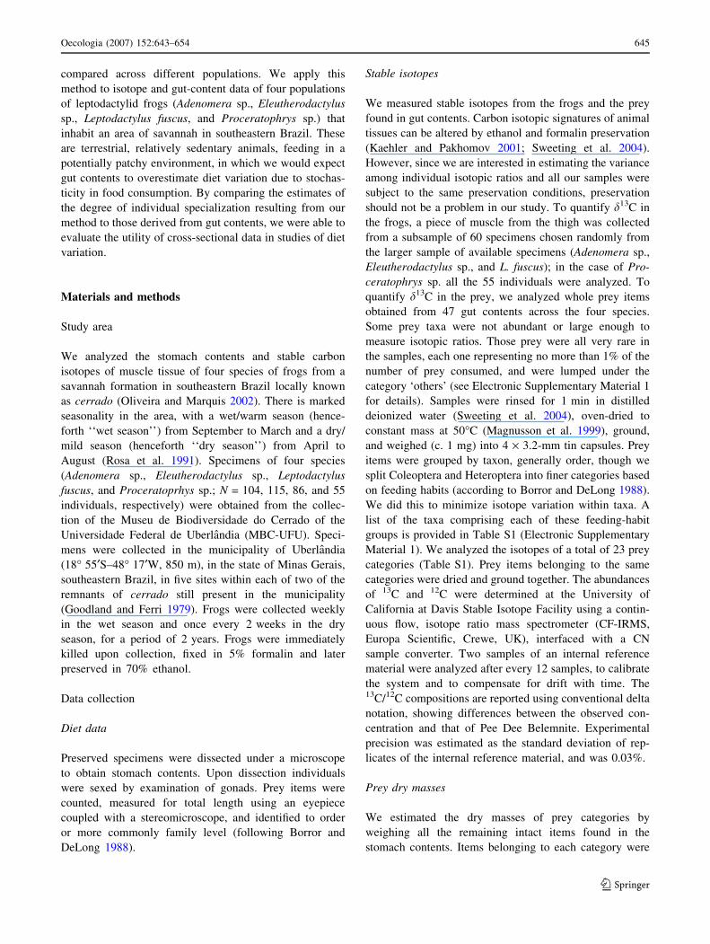
variation. Turning instead to isotope data, we found that
isotope variances ranged from 1.38 (Eleutherodactylus
sp.; Table 1; Fig. 2b) to 8.35 (Proceratophrys sp.; Ta-
ble 1; Fig. 2c). Prey isotopic signatures were also vari-
able, spanning from –24.57 to –13.32& (Table S1;
Fig. 2).
Sex, age, and season had no significant effects on gut
contents or isotopes (Table S2). This indicates that re-
source use differences were not an artifact of collection
season, and that diet variation occurred at the individual
level. We therefore pooled samples by sex, age, and date in
later analyses. However, we did observe an effect of col-
lection site on isotope ratios (Adenomera sp. and L. fuscus;
Table S2) and gut contents (Proceratophrys sp.; Table S2).
In those cases, we did additional post-hoc tests (Tukey) in
order to identify those sites that differed from each other.
Based on these results (not shown), we split samples of
Adenomera sp. and L. fuscus into two subsamples (hence-
forth ss1 and ss2). In the case of Proceratophrys sp., we
removed the sparsely collected site 1 (N = 3 frogs) from
the analyses.
Comparing isotope variation to gut-content variation
Our simulations provided an expected relationship between
WIC/TNW and Vardi (Fig. 3). Using the empirical d13C
variances and this curvilinear relationship, we estimated
values of WIC/TNW (Fig. 3). The values of WIC/TNW
obtained from gut contents consistently fell within the
isotope-derived confidence intervals in Adenomera sp. and
in L. fuscus-ss1, but outside the confidence intervals in
Eleutherodactylus sp., L. fuscus-ss2, and Proceratophrys
sp. (Fig. 3). Contrary to our expectations, stable isotopes
indicated that individual specialization was actually
stronger than we inferred from gut contents in Procera-
tophrys sp. (Fig. 3d). In L. fuscus-ss2 (Fig. 3f), gut con-
tents revealed a higher level of individual specialization
than did the isotopes. Isotopes revealed negligible diet
variation in Eleutherodactylus sp. (Fig. 3c), in stark con-
trast to the gut-content results. Results using the IS index
of individual specialization were qualitatively similar
(Table S3, Fig. S1).
Discussion
Our results show that there is evidence of individual spe-
cialization in the studied populations and that species vary
Table 1 Measures of intra-population variation in food-resource use
in four species of Brazilian frogs
Species WIC/
TNWobs
Vard13C WIC/
TNWexp
Adenomera sp.
ss1 (39) 0.4738*** 5.38 0.3967
ss2 (35) 0.4266*** 4.90 0.4155
Eleutherodactylus sp. (56) 0.4573** 1.38 0.8636
Proceratophrys sp. (49) 0.3700*** 8.35 0.1585
L. fuscus
ss1 (38) 0.4873*** 2.87 0.4965
ss2 (29) 0.4127*** 2.01 0.6419
Numbers in parenthesis are sample sizes. Empirical WIC/TNW val-
ues were tested against null distributions generated with Monte Carlo
bootstraps (1,000 simulations)
WIC/TNWobs Roughgarden’s (1979) index of individual specialization
based on gut-content data, Vard13C empirically estimated isotopic
variances of frog samples, WIC/TNWexp expected value of the index
based on isotope data. L. fuscus Leptodactylus fuscus, ss1 and ss2subsamples 1 and 2, respectively (see text for details)
**P = 0.01, ***P < 0.001
648 Oecologia (2007) 152:643–654
123
in the degree of individual specialization. Surprisingly, gut-
content variation provided fairly good estimates of overall
levels of individual specialization in Adenomera sp. and L.
fuscus. On the other hand, gut contents greatly overesti-
mated individual specialization in Eleutherodactylus sp.
and greatly underestimated it in Proceratophrys sp.
(Fig. 3). In the following discussion, we comment on: (1)
why gut contents and isotopes may over- or underestimate
individual specialization; (2) the impact of missing prey
categories; (3) the impact of the variance in fractionation
among individuals on our method.
Value of gut contents and isotopes in measuring
diet variation
Had we only analyzed gut contents, we would have con-
cluded that the four species had roughly similar degrees of
individual specialization (approximately 0.45). Double-
checking these estimates with comparable isotope-derived
measures of diet variation, we found a moderately close
agreement between gut content and isotope-based mea-
sures of individual specialization in Adenomera sp. and L.
fuscus. This supports the idea that gut-content variation
may be a reasonable measure of diet variation in some
systems, even in the case of terrestrial, relatively sedentary
animals like frogs. However, in two other species gut
contents appear to have yielded misleading measures of
diet variation. For instance, isotopes suggest that Eleut-
herodactylus sp. has a much lower degree of individual
specialization than the other species (expected WIC/
TNW = 0.86). Since there is no a priori way of knowing
how well gut contents will perform, we do not recommend
the use of gut contents alone in studies of individual spe-
cialization, unless individuals are repeatedly sampled over
time. In the case of ‘snapshot’ samples, other measures of
temporal consistency (e.g., morphology and stable iso-
topes) should be used as a complementary approach.
It is reasonably easy to understand how gut contents
would lead one to overestimate levels of individual spe-
cialization (‘false specialists;’ Warburton et al. 1998). If
all individuals had similar preferences (low individual
specialization), one may nevertheless see substantial var-
iation among stomachs due to stochastic effects associated
with patchy prey distributions, or limited stomach volume
so that each consumer holds only a few prey at a time
(Bolnick et al. 2002). This appears to be the case in
Eleutherodactylus sp., since isotopes indicated that there
was far less diet variation than we observed in gut con-
tents (WIC/TNW = 0.86 and 0.46, respectively). Eleut-
herodactylus sp. is a small-sized frog (mean ± SD
SVL = 14.5 ± 2.65 mm; N = 124) with small stomach
capacity (mean ± SD number of prey items per stom-
ach = 4.0 ± 2.42) that is found both on the ground and on
the vegetation (up to 1 m high; A.A. Giaretta personal
observation). These two microhabitats may constitute
different ‘patches’ in terms of prey availability, which
combined with the low stomach capacity of individuals’
generated false specialists.
tnuoC
δ13C (‰)
0
10
20
30
40 a Adenomera sp.
0
10
20
30
40
50
60 b Eleutherodactylus sp.
-35 -30 -25 -20 -150
10
20
30
40 d L. fuscus
-35 -30 -25 -20 -100
10
20
30 c Proceratophrys sp.
-15 -10
Fig. 2 Histograms of the
empirically measured individual
d13C signatures in four species
of Brazilian frogs: a Adenomerasp. (N = 60), bEleutherodactylus sp. (N = 60),
c Proceratophrys sp. (N = 55),
d Leptodactylus fuscus(N = 60). Dashed lines indicate
the range of d13C of consumed
prey
Oecologia (2007) 152:643–654 649
123

It is more difficult to see why stomach contents would
underestimate diet variation as compared to isotope vari-
ance, as in Proceratophrys sp. We propose three possible
explanations for this conflict. First, if prey isotopic signa-
tures vary temporally or spatially, individuals feeding on
the same prey taxa, but collected in different times or
places will show variation in signatures, so that one will
observe isotopic variance that is not actually related to diet
variation (Matthews and Mazumder 2004; Matthews and
Mazumder 2005). In our study, we tried to mitigate this
problem by testing for seasonal and spatial effects on the
consumers’ isotopic ratios, but we acknowledge we cannot
rule out those effects entirely. Ideally, future studies should
strive to assess the seasonal and spatial patterns of variation
in the prey isotopic landscape by sampling prey isotopes in
the field over the seasons and over space. Bearing those
caveats in mind, we did not find any among-site or seasonal
differences in the isotopes of Proceratophrys sp. (Ta-
ble S2), indicating that spatial and seasonal variation in
prey isotopes seems an unlikely explanation for the
apparent conflict between gut contents and isotopes in this
species.
Second, the preservation times before the isotopic
analysis differed among individuals. If there are consistent
shifts in isotopic signatures related to the time of preser-
vation, this could have increased the isotopic variances of
our samples. We tested isotopic signatures of our samples
against time of preservation and found a positive rela-
tionship in Proceratophrys sp. (r2 = 0.133; F1,53 = 8.152;
P = 0.006; Fig. S2), but not in the other species (all P-
values > 0.56; Fig. S2). This significant relationship, albeit
weak, may indicate either an effect of preservation time or
a temporal trend in the prey isotopic ratios. We see the
former as an unlikely explanation for two reasons. First,
Kaehler and Pakhomov (2001) and Sweeting et al. (2004)
observed that after an initial period of isotopic shifts
(4 weeks in the former and 1 day in the latter study) due to
formalin or ethanol preservation of animal tissues, isotopic
signatures remained stable for the whole duration of
experiments (12 weeks in the former and 21 months in the
latter). Since all our samples were analyzed after at least
45 months of preservation, we would not expect to see
such a trend in the isotopic ratios of our samples due to the
effect of preservatives. Second, if preservatives were
Fig. 3 Interpolation of WIC/
TNW from isotope variances:
the values of d13C variances
(Vardi) were regressed onto
measures of individual
specialization (WIC/TNW) of
simulated populations (see text
for details). Solid curvesindicate quadratic fitted
regressions; dashed curves are
the prediction bands of the
regressions; horizontal solidlines indicate the empirically
estimated Vardi; vertical solidlines define the confidence
limits (95%) around the
expected WIC/TNW. Arrowsindicate the expected (Exp)
WIC/TNW interpolated from
the empirical Vardi using the
regression equations and the
observed (Obs) WIC/TNW from
gut contents of four Brazilian
frogs. a Adenomera sp.-ss1
(N = 39), b Adenomera sp.-ss2
(N = 35), c Eleutherodactylussp. (N = 56), d Proceratophryssp. (N = 55), e Leptodactylusfuscus-ss1 (N = 38), fLeptodactylus fuscus-ss2
(N = 29). ss1 and ss2subsamples 1 and 2,
respectively (see text)
650 Oecologia (2007) 152:643–654
123

causing this shift, we would expect to see it in all the four
species, because all samples were subject to the same type
of preservation. We therefore believe it is more likely that
this pattern reflects a temporal trend in one or a few food
sources that were more consumed by Proceratophrys sp.
than the other species (e.g., seeds; Table S1). In either
case, future studies would benefit from standardizing the
time of preservation of samples so that biases in the iso-
topic variance due to preservative-induced isotopic shifts
will be avoided.
Finally, the very low isotope-derived value of WIC/
TNW in Proceratophrys sp. might be a result of under-
sampling prey isotope variation (see below). It is likely that
some individuals in our sample fed on some unknown prey
with isotope signatures outside the range of what we ob-
served in the most common prey. This is because some
individual frogs had isotope signatures outside the range of
prey isotopes (Fig. 2), and in Proceratophrys sp. the
number of isotopic outliers was higher than in the other
species (Fig. 2).
The mismatch between frogs’ and prey signatures in our
samples may have several reasons. First, consumers may
show shifts in d13C in relation to their food sources due to
fractionation (Vander Zanden and Rasmussen 2001). Sec-
ond, we may have lacked the taxonomic resolution that
would have allowed us to measure all the isotopic range of
the consumed prey. While we made an effort in trying to
avoid lumping ecologically divergent prey types into a
single category, our taxonomic resolution (23 prey taxo-
nomic categories, some including many families) almost
certainly mixed prey with different signatures. The esti-
mated average values for each category therefore masks a
potentially higher variation among member taxa. It is
possible that the prey signatures that would encompass all
frog signatures in our samples are among these lumped
taxa. Third, we may have actually missed some prey taxa in
our sample. In principle, this should not be a likely
explanation, given our large sample sizes. Moreover, we
would not expect those missing prey types to be used
frequently enough to strongly influence the frogs’ isotopic
ratios. This argument also holds for the taxa lumped under
the category ‘others,’ which were not included in the iso-
tope analyses for lack of material. None of these taxa ac-
counted for more than 1% of prey items within any species’
diet. Interestingly, however, in the case of Proceratophrys
sp., all isotopic outliers are small juveniles (all below the
25th percentile of SVL). Differently from the other studied
species, Proceratophrys sp. reproduces in permanent
streams and has a long (many weeks; Giaretta A.A.
unpublished results) aquatic larval development, whereas
Adenomera sp. and Eleutherodactylus sp. have totally ter-
restrial development, and L. fuscus has a very short
(2 weeks maximum) aquatic larval phase (Kokubum and
Giaretta 2005; Giaretta A.A. unpublished results). The
feeding habits of the larvae of Proceratophrys sp. are un-
known, but the diet of tadpoles may well include isotopi-
cally depleted sources found in the aquatic environment
(Matthews and Mazumder 2005; Paterson et al. 2006).
Since we only sampled prey consumed in the terrestrial
environment, this would explain why the isotopic range in
this species was much larger than that of the sampled prey.
Impact of missing prey categories
Our simulation model is based on the assumption that we
have a sufficient sample of prey taxa to generate a real-
istic relationship between WIC/TNW and Vardi. Under-
estimating the true variance in prey isotopes could lead to
spurious estimates of WIC/TNW. To understand why this
is the case, consider the y-intercept of the simulated
curves (Fig. 3). This is the isotopic variance when each
individual uses a single prey type (hence WIC/TNW = 0),
and will be equal to the variance in the empirically
determined prey isotopes (weighted by prey frequency in
the population diet). Consequently, greater variances in
the estimated prey isotopes will generate steeper regres-
sion curves. If one underestimates the true prey isotope
variance (due to the problems discussed above), the
simulated curve will be lower than it should actually be
(Fig. 4a). As a result, a given empirical value of Vardi
will lead to an interpolated WIC/TNW that is too low
(overestimating individual specialization; Fig. 4a). This
observation is of utmost importance for our results, be-
cause we used empirically estimated d13C variances to
generate expected values of WIC/TNW. If we underesti-
mated the variance in prey isotopes, as suggested by the
isotopic outliers in Proceratophrys sp., then our regres-
sion curves are less steep than they should be, and we
might have overestimated the degree of individual spe-
cialization. Conversely, overestimating prey variances, for
instance by missing isotopically intermediate prey, will
lead to an underestimate of individual specialization
(higher WIC/TNW).
In light of these biases, our interpolation technique is
most appropriate when isotope data are available for all
prey taxa. This was not possible in this study due to the
coarse taxonomic resolution for observed prey and/or our
inability to ensure that all prey taxa were accounted for.
Since we are unable to determine which prey isotope val-
ues we are missing, we took another approach to evaluating
the impact of missing prey on our results. We redid our
analysis of Proceratophrys sp., eliminating the individual
frogs whose isotope signatures could not be explained by
the observed prey isotopes (see Electronic Supplementary
Material 5 for details). Eliminating the ten isotopic outliers
reduced the d13C variance from 8.35 to 3.32, but did not
Oecologia (2007) 152:643–654 651
123

effectively change the gut-content estimates of WIC/TNW
(0.37 vs. 0.38). In contrast, the isotope-derived estimates of
WIC/TNW increased from 0.16 to 0.52, coming closer in
line with the gut-content estimates and the values for two
of the other species (Table S4, Fig. S3). This supports our
view that the low isotope-derived value of WIC/TNW
observed in Proceratophrys sp. may be a result of insuf-
ficient data on prey isotopes. Similar reanalysis increased
the estimates of WIC/TNW of Adenomera sp. from
approximately 0.40 to approximately 0.55 and had negli-
gible effects on results for the other species (Electronic
Supplementary Material 5), which had fewer isotopic
outliers.
Impact of the variation in fractionation among
individuals
As mentioned earlier, differential assimilation, fraction-
ation, and isotopic routing may all cause a mismatch
between signatures of food sources and those of con-
sumers. More important, if there is variation among
individuals in, e.g., fractionation, the population isotopic
variance will be higher than would be expected based
solely on diet variation (Matthews and Mazumder 2005).
As a way of assessing the impact of fractionation on our
model, we did simulations incorporating among-individ-
ual variance in fractionation (VarD). We computed from
the literature empirical measures of variation in fraction-
ation among individuals fed on the same diet. We used an
average VarD = 0.73 based on 12 such variances, 9 from
the gerbil Meriones unguienlatus (Tieszen et al. 1983)
and one from each of three bird species, the quail Co-
turnix japonica, the chicken Gallus gallus, and the gull
Larus delawarensis (Hobson and Clark 1992). We ran
simulations in which a fractionation value drawn ran-
domly from a uniform distribution with variance 0.73
(range 0–2.96) was added to an individual’s isotopic
signature. In these simulations, sample size was set at
N = 30, population diet was (0.2, 0.2, 0.2, 0.2, 0.2) and
prey isotopes were (–31, –30, –29, –28, –27). The
incorporation of VarD in our model caused an upward
shift in the resulting curve, so that even in the absence of
diet variation (WIC/TNW = 1), there was a baseline iso-
topic variation (Fig. 4b). Interestingly, the difference be-
tween the y-values of this curve and that of a control
curve generated with the same set of parameters, but no
fractionation, corresponds to approximately VarD
(Fig. 4b). Additional simulations changing the value of
VarD (0.5 and 1.0) and the prey isotope range (–34, –32, –
30, –28, –26) did not change this pattern. Therefore, if
one has an estimate of VarD for the studied organism, it is
possible to correct its effect on the results of the model by
subtracting VarD from the empirical Vardi before inter-
polating the expected value of WIC/TNW (Fig. 4b).
Using VarD = 0.73 as a correction for our samples, the
expected WIC/TNW values increased by 0.05–0.1, indi-
cating less diet variation. The change was not substantial,
though, and there is still evidence of diet variation in
three of the four species. It is worth mentioning that
empirical estimates of VarD may vary considerably among
different taxonomic groups (e.g., gerbils = 1.01;
birds = 0.4; average values). A more realistic estimate in
the case of frogs might be quite different from 0.73.
Conclusions
Gut contents may be a useful source of information on
individual-level diet variation, especially if coupled with
raV
δ i
Empirical Varδi
InferredActual
a
WIC/TNW
Empirical Varδi
Inferred
Actual Var∆
Corrected Varδi
b
Fig. 4 Illustration of the effect of a incomplete sampling of prey on
our model, and b variation in fractionation among individuals, based
on simulations. a The solid curve represents the ‘‘true’’ relationship
for a hypothetical prey community, while the dotted curve represents
the relationship that is inferred from an incomplete sample of prey
that missed isotopically extreme taxa and so underestimates the prey
isotope variance. Using this incomplete dataset, one would infer an
excessively low value of WIC/TNW. b Solid curve as in a, but now
assuming that individuals vary in fractionation, while in the dottedcurve no fractionation is assumed. By denying the among-individual
variance in fractionation (VarD), one would also underestimate WIC/
TNW. However, if an empirical estimate of VarD is available, it is
possible to correct the estimate of WIC/TNW by using a ‘‘corrected’’
Vardi, where corrected Vardi = empirical Var di – VarD
652 Oecologia (2007) 152:643–654
123

data on stable isotopes. Information on the population d13C
variance, combined with information on prey isotopes, can
be a useful tool to test for the presence of individual spe-
cialization (Matthews and Mazumder 2004). The model
presented here goes a step further by providing a way to
generate, from information on isotopic variances, estimates
of standardized indices of individual specialization (Bol-
nick et al. 2002) that can be compared among different
populations or used to evaluate gut-content variation in
different species and/or systems. This method requires
thorough sampling of the isotope ratios of the prey com-
munity, but is otherwise straightforward. Individual spe-
cialization is a phenomenon with important ecological and
evolutionary implications for populations. In a review of
the incidence of individual specialization, Bolnick et al.
(2003) make the case that most studies on individual spe-
cialization up to now were only able to test the null
hypothesis that individuals in a population are all gener-
alists and that we should be able to actually measure and
compare the degrees of individual specialization across
different populations. For instance, it is still unclear how
widespread this phenomenon is among natural populations,
as well as what ecological conditions will favor its evolu-
tion and maintenance. Quantifying individual specializa-
tion in a comparable manner is a necessary step in any
attempt to answer these questions.
Acknowledgments We thank IBAMA for permit numbers
0121586BR and 0123253BR. J.Y. Tamashiro and A.J. Santos helped
in the identification of some of the prey items. We thank J.P.H.B.
Ometto for fruitful discussions. L. Marschall, B. Matthews, and two
anonymous reviewers made useful suggestions that greatly improved
the manuscript. M.S.A. thanks CAPES, and S.F.R. and A.A.G. thank
CNPq for fellowships. Financial support was provided by FAPESP,
CAPES, FAPEMIG, and an NSF grant #DEB-0412802 to DIB.
References
Angerbjorn A, Hersteinsson P, Liden K, Nelson E (1994) Dietary
variation in arctic foxes (Alopex lagopus)—an analysis of stable
carbon isotopes. Oecologia 99:226–232
Bolnick DI (2004) Can intraspecific competition drive disruptive
selection? An experimental test in natural populations of
sticklebacks. Evolution 58:608–618
Bolnick DI, Yang LH, Fordyce JA, Davis JM, Svanback R (2002)
Measuring individual-level resource specialization. Ecology
83:2936–2941
Bolnick DI et al (2003) The ecology of individuals: incidence and
implications of individual specialization. Am Nat 161:1–28
Borror JD, DeLong DM (1988) Introducao ao estudo dos insetos.
Edgar Bluchet Ltda., Sao Paulo
Bryan JE, Larkin PA (1972) Food specialization by individual trout.
J Fish Res Board Can 29:1615–1624
Dalerum F, Angerbjorn A (2005) Resolving temporal variation in
vertebrate diets using naturally occuring stable isotopes. Oeco-
logia 144:647–658
Dieckmann U, Doebeli M (1999) On the origin of species by
sympatric speciation. Nature 400:354–357
Durell SE (2000) Individual feeding specialisation in shorebirds:
population consequences and conservation implications. Biol
Rev 75:503–518
Fermon Y, Cibert C (1998) Ecomorphological individual variation in
a population of Haplochromis nyererei from the Tanzanian part
of Lake Victoria. J Fish Biol 53:66–83
Fry B, Joern A, Parker PL (1978) Grasshopper food web analysis: use
of carbon isotope ratios to examine feeding relationships among
terrestrial herbivores. Ecology 59:498–506
Gannes LZ, O’Brien DM, del Rio CM (1997) Stable isotopes in
animal ecology: assumptions, caveats, and a call for more
laboratory experiments. Ecology 78:1271–1276
Goodland R, Ferri GM (1979) Ecologia do Cerrado. Livraria Itatiaia,
Belo Horizonte
Gu B, Schelske CL, Hoyer MV (1997) Intrapopulation feeding
diversity in blue tilapia: evidence from stable-isotope analyses.
Ecology 78:2263–2266
Heinrich B (1979) ‘‘Majoring’’ and ‘‘minoring’’ by foraging
bumblebees, Bombus vagans: an experimental analysis. Ecology
60:245–255
Hobson KA, Clark RG (1992) Assessing avian diets using stable
isotopes II: factors influencing diet-tissue fractionation. Condor
94:189–197
Hodar JA (1996) The use of regression equations for estimation of
arthropod biomass in ecological studies. Acta Oecol 17:421–433
Kaehler S, Pakhomov EA (2001) Effects of storage and preservation
on the d13C and d15N signatures of selected marine organisms.
Mar Ecol Prog Ser 219:299–304
Kokubum MNDC, Giaretta AA (2005) Reproductive ecology and
behaviour of a species of Adenomera (Anura, Leptodactylidae)
with endotrophic tadpoles: systematic implications. J Nat His
39:1745–1758
Lomnicki A (1992) Population ecology from the individual perpec-
tive. In: DeAngelis DL, Gross LJ (eds) Individual-based models
and approaches in ecology. Routledge/Chapman & Hall,
London/New York, pp 3–17
Magnusson WE et al (1999) Contributions of C3 and C4 plants
to higher trophic levels in an Amazonian savanna. Oecologia
119
Matthews B, Mazumder A (2004) A critical evaluation of intrapop-
ulation variation of d13C and isotopic evidence of individual
specialization. Oecologia 140:361–371
Matthews B, Mazumder A (2005) Consequences of large temporal
variability of zooplankton d15N for modeling fish tropic position
and variation. Limnol Oceanogr 50:1404–1414
Oliveira PS, Marquis RJ (2002) (eds) The cerrados of Brazil: ecology
and natural history of a neotropical savanna. Columbia Univer-
sity Press, New York
Paterson G, Drouillard KG, Haffner GD (2006) Quantifying resource
partitioning in centrarchids with stable isotope analysis. Limnol
Oceanogr 51:1038–1044
Phillips DL, Gregg JW (2003) Source partitioning using stable
isotopes: coping with too many sources. Oecologia 136:261–269
Polis GA (1984) Age structure component of niche width and intra-
specific resource partitioning: can age groups function as
ecological species? Am Nat 123:541–564
Price T (1987) Diet variation in a population of Darwin’s finches.
Ecology 68:1015–1028
Robinson BW, Wilson DS, Margosian AS, Lotito PT (1993)
Ecological and morphological differentiation of pumpkinseed
sunfish in lakes without bluegill sunfish. Evol Ecol 7:451–464
Rosa R, Lima SCC, Assuncao WL (1991) Abordagem preliminar das
condicoes climaticas de Uberlandia (MG). Sociedade e Natureza
3:91–108
Roughgarden J (1972) Evolution of niche width. Am Nat 106:683–
718
Oecologia (2007) 152:643–654 653
123

Roughgarden J (1974) Niche width: biogeographic patterns among
Anolis lizard populations. Am Nat 108:429–442
Roughgarden J (1979) Theory of population genetics and evolution-
ary ecology: an introduction. Macmillan, New York
Sample BE, Cooper RJ, Greer RD, Whitmore RC (1992) Estimation of
insect biomass by length and width. Am Midl Nat 129:234–240
Schindler DE (1997) Density-dependent changes in individual
foraging specialization of largemouth bass. Oecologia
110:592–600
Slatkin M (1984) Ecological causes of sexual dimorphism. Evolution
38:622–630
Svanback R, Bolnick DI (2005) Intraspecific competition affects the
strength of individual specialization: an optimal diet theory
model. Evol Ecol Res 7:993–1012
Swanson BO, Gibb AC, Marks JC, Hendrickson DA (2003) Trophic
polymorphism and behavioral differences decrease intraspecific
competition in a cichilid, Herichthys minckleyi. Ecology
84:1441–1446
Sweeting CJ, Polunin NVC, Jennings S (2004) Tissue and fixative
dependent shifts of d13C and d15N in preserved ecological
material. Rapid Commun Mass Spectrom 18:2587–2592
Sweeting CJ, Jennings S, Polunin NVC (2005) Variance in isotopic
signatures as a descriptor of tissue turnover and degree of
omnivory. Funct Ecol 19:777–784
Taper ML, Case TJ (1985) Quantitative genetic models for the
coevolution of character displacement. Ecology 66:355–371
Tieszen LL, Boutton TW, Tesdahl KG, Slade NA (1983) Fraction-
ation and turnover of stable carbon isotopes in animal tissues:
implications for d13C analysis of diet. Oecologia 57:32–37
Van Valen L (1965) Morphological variation and width of ecological
niche. Am Nat 99:377–390
Vander Zanden MJ, Rasmussen JB (2001) Variation in d15N and
d13C trophic fractionation: implications for aquatic food web
studies. Limnol Oceanogr 46
Warburton K, Retif S, Hume D (1998) Generalists as sequential
specialists: diets and prey switching in juvenile silver perch.
Environ Biol Fish 51:445–454
Werner TK, Sherry TW (1987) Behavioral feeding specialization in
Pinaroloxias inornata, the ‘‘Darwin’s Finch’’ of Cocos Island,
Costa Rica. Proc Natl Acad Sci USA 84:5506–5510
654 Oecologia (2007) 152:643–654
123


