Embed Size (px)
Citation preview
University of Montana University of Montana
ScholarWorks at University of Montana ScholarWorks at University of Montana
Graduate Student Theses, Dissertations, & Professional Papers Graduate School
2001
Using honey bees and thermal desorption/gas chromatography/Using honey bees and thermal desorption/gas chromatography/
mass spectrometry to assess the regional distribution of mass spectrometry to assess the regional distribution of
bioavailable volatile organic compounds in northeast Maryland bioavailable volatile organic compounds in northeast Maryland
David C. Jones The University of Montana
Follow this and additional works at: https://scholarworks.umt.edu/etd
Let us know how access to this document benefits you.
Recommended Citation Recommended Citation Jones, David C., "Using honey bees and thermal desorption/gas chromatography/mass spectrometry to assess the regional distribution of bioavailable volatile organic compounds in northeast Maryland" (2001). Graduate Student Theses, Dissertations, & Professional Papers. 9148. https://scholarworks.umt.edu/etd/9148
This Thesis is brought to you for free and open access by the Graduate School at ScholarWorks at University of Montana. It has been accepted for inclusion in Graduate Student Theses, Dissertations, & Professional Papers by an authorized administrator of ScholarWorks at University of Montana. For more information, please contact [email protected].
The University of
MontanaPermission is granted by the author to reproduce this material in its entirety, provided that this material is used for scholarly purposes and is properly cited in published works and reports.
**Please check "Yes” or ”No" and provide signature**
Yes, I grant permission
No, I do not grant permission
Author’s Signature: ^
Date: _ r
Any copying for commercial purposes or financial gain may be undertaken only with the author’s explicit consent.
8/98

Using Honey Bees and Thermal Desorption / Gas Chromatography / Mass Spectrometry to A ssess the Regional Distribution of Bioavailable Volatile
Organic Compounds in Northeast Maryland
by
David C. Jones
B.S. Idaho State University, Pocatello, Idaho, 1986
Presented in partial fulfillment of the requirements
of the degree
Masters in Science in Chemistry
The University of Montana
August, 2001
Approved by
Board of
Dean, Graduate School
Date
UMI Number: EP39949
All rights reserved
INFORMATION TO ALL USERS The quality of this reproduction is dependent upon the quality o f the copy submitted.
In the unlikely event that the author did not send a complete m anuscript and there are missing pages, these will be noted. Also, if material had to be removed,
a note will indicate the deletion.
UMID is sâ r la tio n Publish«f>g
UMI EP39949
Published by ProQuest LLC (2013). Copyright in the Dissertation held by the Author.
M icroform Edition © ProQuest LLC.All rights reserved. This work is protected against
unauthorized copying under Title 17, United States Code
uestProQuest LLC.
789 East Eisenhower Parkway P.O. Box 1346
Ann Arbor, MI 4 8 1 0 6 - 1346
Jones, David C. M .S. August, 2001 Chemistry
Using Honey Bees and Thermal Desorption/Gas Chromatography/Mass Spectrometry to Assess the Regional Distribution of Bioavailable Volatile Organic Compounds in Northeast Maryland
Advisor: Garon C. Smith G a s
Honey bee colonies were used to identify potential sources of bioavailable, priority pollutant, volatile organic compounds. Bioavailable pollutants are those in the environment that can be assimillated by any organisms when contacted by them. Our objective was to determine if an army base-Aberdeen Proving Ground (APG) in Maryland-was the main source of these contaminants. Paired bee hives were set up on three, nine and twenty-one mile radii along three main transects: north, northwest and southwest. Using constant flow air pumps and carbon-based chemical traps, samples were taken from the hive air and outside air at each site. Samples were analyzed using thermal desorption/gas chromatography/mass spectrometry (TD/GC/MS). Concentrations were quantified for ten compounds - four halogenated organics representing industrial solvents, and six aromatic hydrocarbons, representing four persistant petroleum fuel residues and two tear gas residues. The data was reduced using three methods: Chronic Exposure, Acute Exposure Ranking, and an Analysis of Variance. Results demonstrate that the army base is not the major source of the priority pollutants, but that the pollutants correlate directly with multiple, local sources. These include vehicle exhaust, fugitive fossil fuel emissions, household products, agrochemicals, and industrial reagents. Comparisons between the 1998 and 1999 field seasons are made.
u
AcknowledgementsI ’d like to thank and acknowledge the many individuals whose efforts went into the completion of this thesis. Dr. Garon Smith for luring me into the “bee project”, for his years of patience and guidance, and for his mentorship. My committee members Dr. Jerry Bromenshenk for his enthusiasm, drive and support and Dr. Mark Craciolice for “Zen-like” calmness, good humor, and friendship.
Thanks to Dr. Colin Henderson for his help setting up, running, and checking the statistics for this project.
To my Lab 05 mates Tony Ward, Chris Wrobel, and Bruce King for their friendship and expertise, without whom the challenge of a project like this would have been unrealized.To Mark Mencel for his sample analysis, enthusiasm for climbing and willingness to do the grunt work.
To the BeeAlert! crew especially Lenny Hahn, Chief Bee Wrangler, Jason Volkman ’98 Maryland crew, ‘T he Kiwis” Michelle and Byron Taylor the ’99 Maryland crew, David Hooper head work-study.
To Dr. Edward Rosenberg, Department Chair of Chemistry, and the rest of the Department of Chemistry faculty and staff especially Bonnie Gatewood, Barbara McCann, and Rosalyn Chaitoff, without whom no thesis would get done.
To my Big Sky High School colleagues Jim Harkins, Brett Taylor, Robin Anderson and David Oberbillig for their support and understanding of my absent-mindedness through these past few years.
To Steve Earle for sharing his yawlp and diverse musical talent these last several write-it-up weeks.
To Jennifer Carey my Production Editor, life-partner and best friend. Thanks for helping me keep it all in perspective .. .and fun.
Most importantly, I thank the many bees who consistently went about their business completely oblivious to my efforts.
This work was supported by Contract DAMD17-95-C-5072, U.S. Army Medical Research and Matériels Command, Ft. Detrick, MD, and a Partners in Science Grant from The Research Corporation / M.J. Murdock Charitable Trust.
m
Table o f Contents
Abstract.......................................................................................................................................... li
Acknowledgements......................................................................................................................iii
Table of Contents.........................................................................................................................iv
List of Tables................................................................................................................................. v
List of Figures.............................................................................................................................. vi
Chapter 1: Introduction and Statement of the Problem............................................................. 1
Chapter 2: Experimental Method...............................................................................................11
Chapter 3: Results.......................................................................................................................29
Chapter 4: Discussion, Conclusions and Suggestions for Further Study........................... 65
References.................................................................................................................................... 84
Appendices...................................................................................................................................90
IV
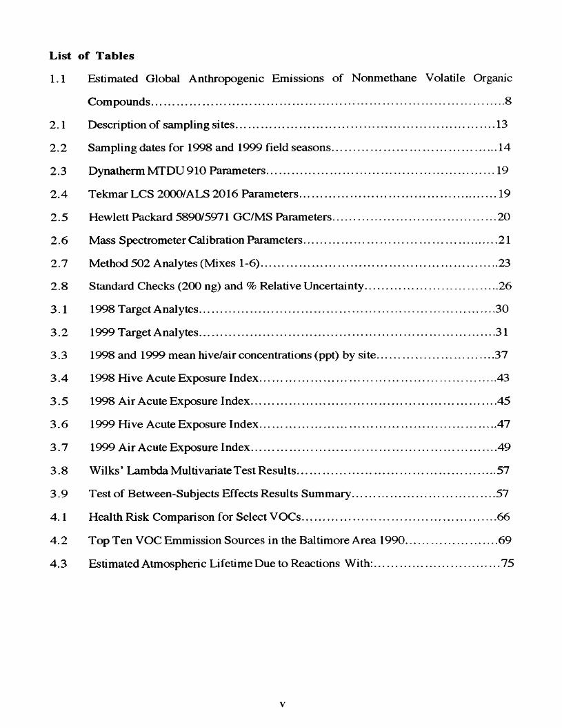
List of Tables
1.1 Estimated Global Anthropogenic Emissions of Nonmethane Volatile Organic
Compounds...................................................................................................................... 8
2.1 Description of sampling sites........................................................................................ 13
2.2 Sampling dates for 1998 and 1999 field seasons.........................................................14
2.3 Dynatherm MTDU 910 Parameters.............................................................................. 19
2.4 Tekmar LCS 2GGG/ALS 2016 Parameters....................................................................19
2.5 Hewlett Packard 5890/5971 GC/MS Parameters........................................................ 20
2.6 Mass Spectrometer Calibration Parameters.................................................................. 21
2.7 Method 502 Analytes (Mixes 1-6).................................................................................23
2.8 Standard Checks (200 ng) and % Relative Uncertainty.............................................. 26
3.1 1998 Target Analytes....................................................................................................30
3.2 1999 Target Analytes....................................................................................................31
3.3 1998 and 1999 mean hive/air concentrations (ppt) by site........................................ 37
3.4 1998 Hive Acute Exposure Index................................................................................ 43
3.5 1998 Air Acute Exposure Index................................................................................... 45
3.6 1999 Hive Acute Exposure Index................................................................................ 47
3.7 1999 Air Acute Exposure Index................................................................................... 49
3.8 Wilks’ Lambda Multivariate Test Results.................................................................... 57
3.9 Test of Between-Subjects Effects Results Summary................................................. 57
4.1 Health Risk Comparison for Select VOCs.................................................................. 66
4.2 Top Ten VOC Emmission Sources in the Baltimore Area 1990................................69
4.3 Estimated Atmospheric Lifetime Due to Reactions With:........................................... 75
List of Figures
1.1 Aberdeen Proving Ground Location Map..................................................................... 2
1.2 J-Field explosives testing 1961...................................................................................... 3
1.3 J-Field disposal work circa 1960................................................................................... 5
1.4 J-Field disposal pit circa 1960........................................................................................6
2.1 Map of study area with directional headings and concentric radii............................. 12
2.2 Schematic of a JAG Box sampling train.......................................................................17
2.3 Wrobel Flash Volatilizer................................................................................................23
3.1 1998 Hive vs Air Mean Concentrations-On Base and Radii.....................................33
3.2 1999 Halogenated Compounds Hive vs Air Mean Concentrations...........................34
3.3 1999 Aromatic Compounds Hive vs Air Mean Concentrations................................ 35
3.4 1,1,1 TCA Total Ion Concentration vs Time...............................................................39
3.5 1,1,2 TCA Total Ion Concentration vs Time...............................................................40
3.6 1998 and 1999 Acute Exposure Index.........................................................................51
3.7 1998 and 1999 Normalized Acute Exposure Index....................................................52
3.8 Study area and assigned coding for ANOVA..............................................................55
3.9 Marginal Means for PC-1 Zone*Heading....................................................................59
3.10 Marginal Means for PC-1 Zone*Heading*Month-July..............................................60
3.11 Marginal Means for PC-1 Zone*Heading*Month-September................................. 61
3.12 Marginal Means for PC-4 Zone*Heading....................................................................62
3.13 Marginal Means for PC-4 Zone*Heading*Month-July..............................................63
3.14 Marginal Means for PC-4 Zone* Headi ng* Month-September...................................64
4.1 Prevailing wind direction...............................................................................................77
VI
CHAPTER 1: P^TRODUCTION AND STATEMENT OF PROBLEM
Introduction
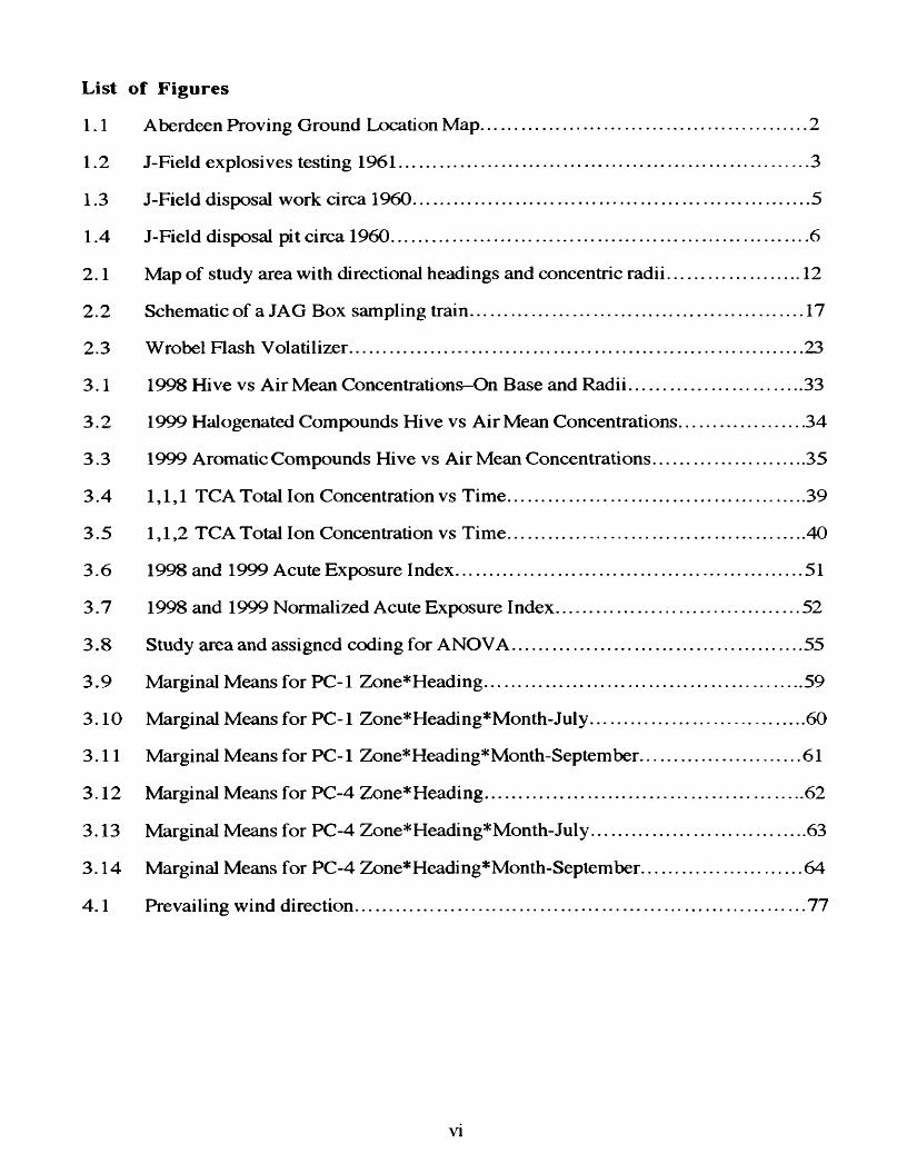
Aberdeen Proving Ground (APG) is an U.S. Department of the Army installation
about 22 miles (35.5 kilometers) northeast of Baltimore, Maryland. The proving ground
occupies several peninsulas and islands that extend into Chesapeake Bay covering a total
area of 79,000 acres (31971 hectare) of land and water. The Bush River divides the
proving ground into two main areas, the Aberdeen Area and the Edgewood Area. Several
small residential areas and the towns of Bel Aire, Abingdon, Edgewood,
Joppatowne/Magnolia, Aberdeen, and Perryman surround APG. The vegetative cover of
the proving ground is primarily thick hardwood forest interspersed with meadows and
estuaries (Bromenshenk et al. 1997,1998; Burges et al. 2000). Figure 1.1 is a map of the
area.
A presidential proclamation appropriated the Edgewood Area for a U.S. Army
proving ground in 1917. Since then, the primary mission of APG has been the
development of weapons systems, munitions, and several military support operations. A
combination of army barracks, houses, offices, and laboratories form the base
infrastructure. Most of the historical activities included weapons research, development,
and field testing, and pilot-scale and production-scale manufacture of chemical warfare
agents. Chemical warfare material, hazardous wastes, and low-level radioactive wastes
have been stored at APG. Weapons development, manufacturing, and testing peaked
during World War II, but limited activity continued until 1971.
PEWNmmNiA
J E R S E YABERDEEN P R O V ifG y
\ GROJUmMARYLAND
4
WV-'v
DELAWARE
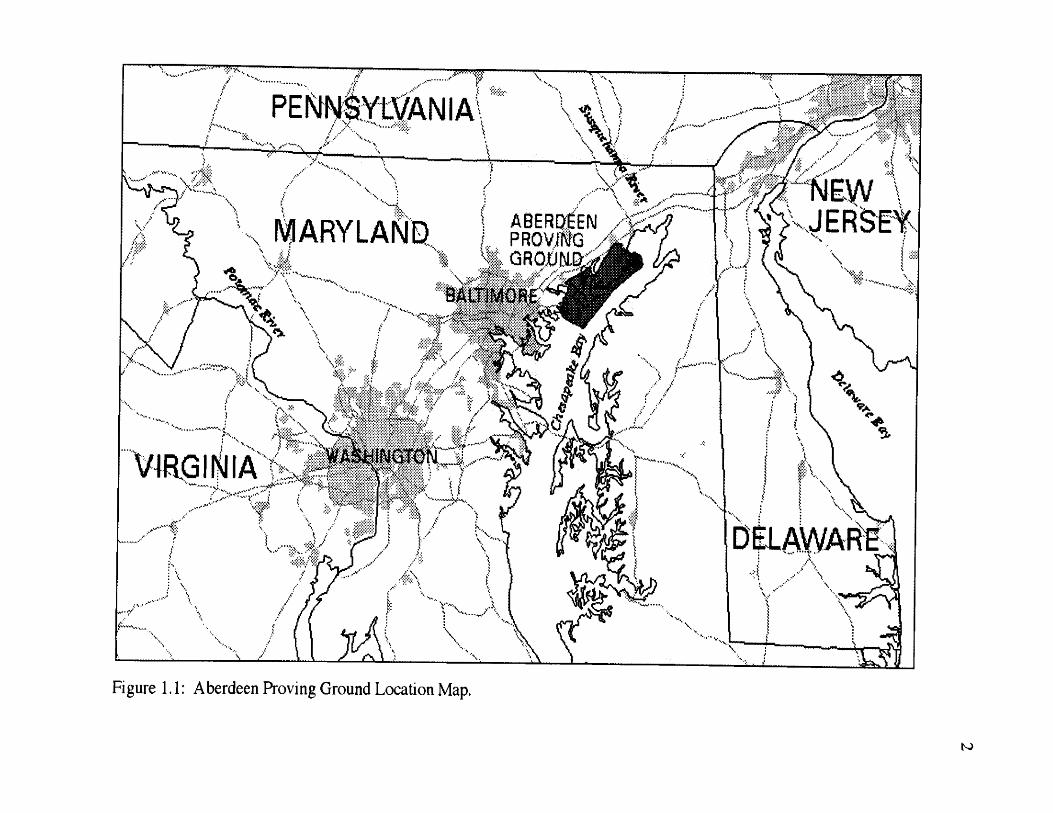
Figure 1.1: Aberdeen Proving Ground Location Map.
0
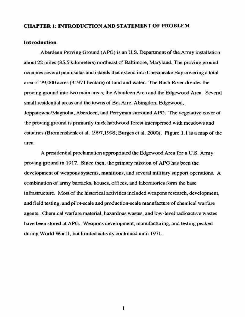
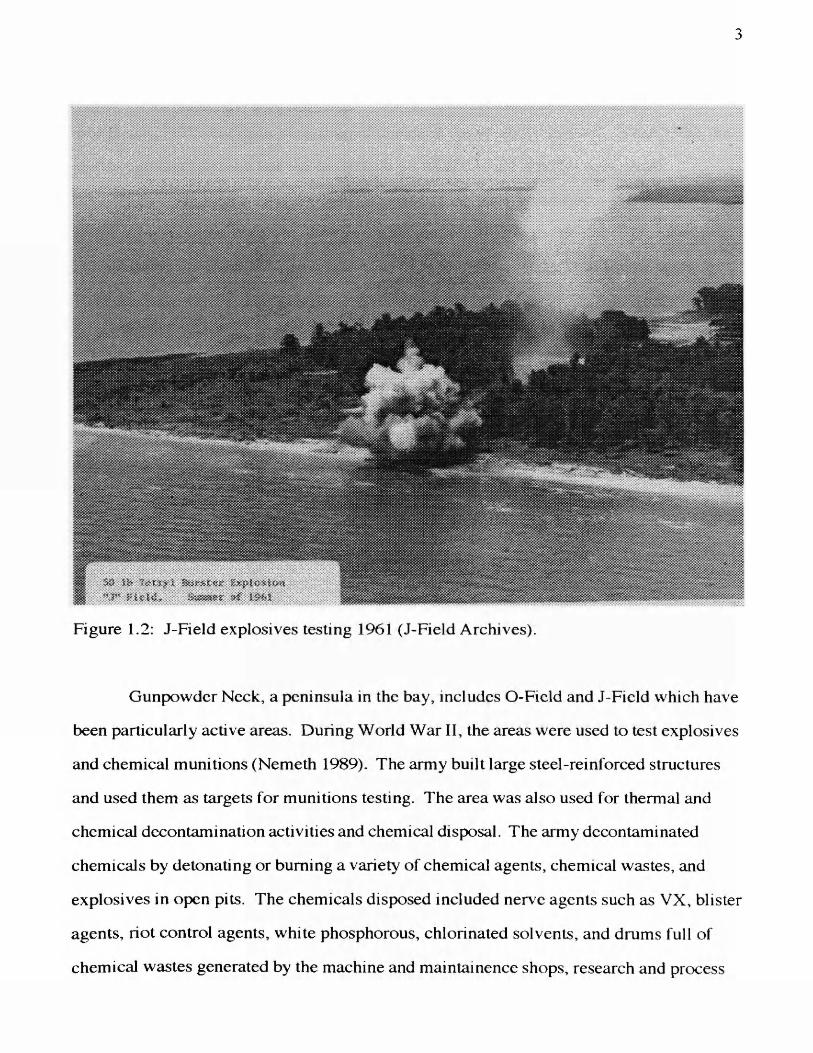
Figure 1.2: J-Field explosives testing 1961 (J-Field Archives).
Gunpowder Neck, a peninsula in the bay, includes O-Field and J-Field which have
been particularly active areas. During World War II, the areas were used to test explosives
and chemical munitions (Nemeth 1989). The army built large steel-reinforced structures
and used them as targets for munitions testing. The area was also used for thermal and
chemical decontamination activities and chemical disposal. The army decontaminated
chemicals by detonating or burning a variety of chemical agents, chemical wastes, and
explosives in open pits. The chemicals disposed included nerve agents such as VX, blister
agents, riot control agents, white phosphorous, chlorinated solvents, and drums full of
chemical wastes generated by the machine and maintainence shops, research and process
laboratories, and pilot plants. Limited testing of chemical agents continued after World
War II until 1971, but open-air testing of chemical agents ended in 1969. Since 1980, the
proving ground has seen limited use though portions are still used for occasional
destruction of explosive-related materials as part of the Installation Recovery and
Restoration Program under the 1984 and 1986 amendments to the Resource Conservation
and Recovery Act (RCRA). First passed in 1976, RCRA gave the U.S. Environmental
Protection Agency the authority to control hazardous waste from the “cradle-to-grave”
including generation, transportation, treatment, storage, and disposal (U.S. EPA 1999) and
applies to both private and government installations. The 1984 amendments to RCRA are
the Federal Hazardous and Solid Waste Amendments required phasing out the land
disposal of hazardous wastes. The 1986 amendments gave the EPA the ability to address
problems associated with the underground storage of petroleum and other hazardous
wastes (McCarthy 1999).
" y' :
: !::;':":::V:::::':$:-r%::%x
:-Æ:':-?S:ÿ;
M # a s s =
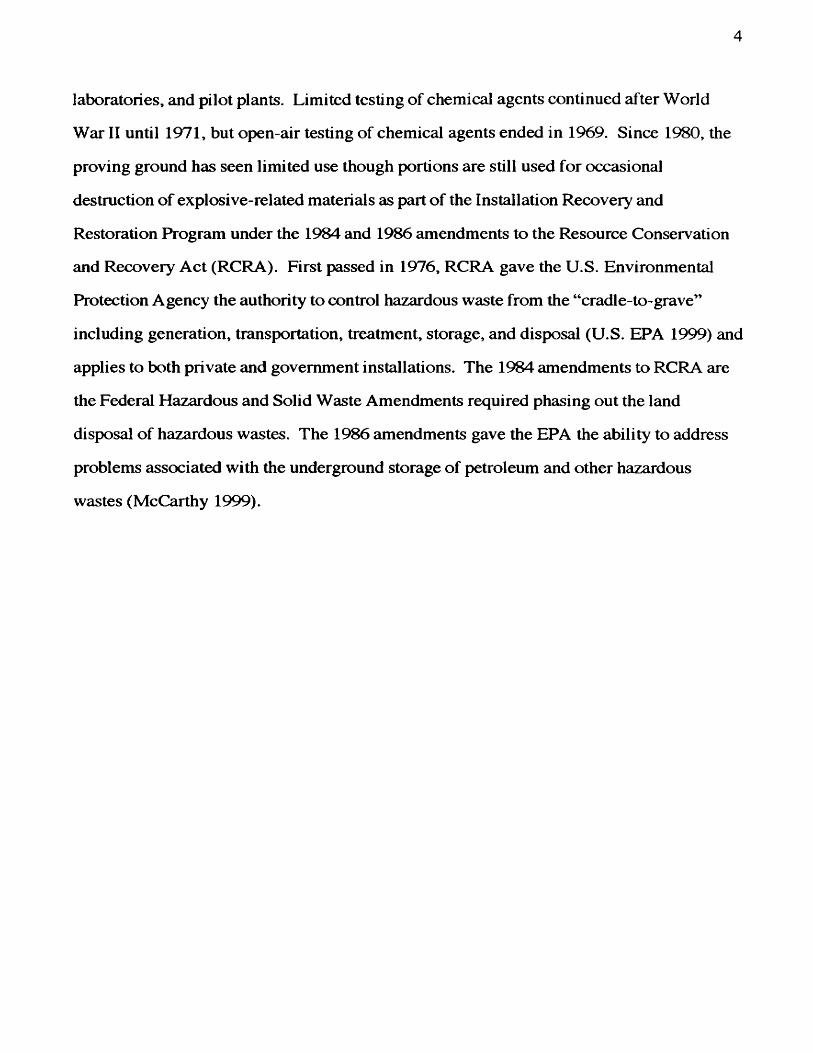
Figure 13: J-Field disposal work circa 1960 (J-Field Archives).
Historical use of industrial solvents and the degradation of products such as rocket
fuel, pyrotechnics, and nerve gas has contaminated the soil and groundwater in localized
areas of the base including decommissioned chemical weapons laboratories,
decommissioned chemical plants, and hazardous waste landfills. Many of the toxic
contaminants are volatile organic compounds (VOCs). Benzene, a VOC, was used as a
solvent, and is listed as a known human carcinogen (Merck Index 1976; American
Conference of Governmental Industrial Hygienists 1995) Toluene and ethyl benzene, also
VOCs, are less toxic but will easily react to form more toxic products (Singh et al. 1992).
Since 1997, Weston Inc., General Physics Inc., and Argonne National Laboratory have
modeled groundwater flow and conducted studies to determine the feasibility and
effectiveness of treating volatile organic compounds (Argonne 1998).
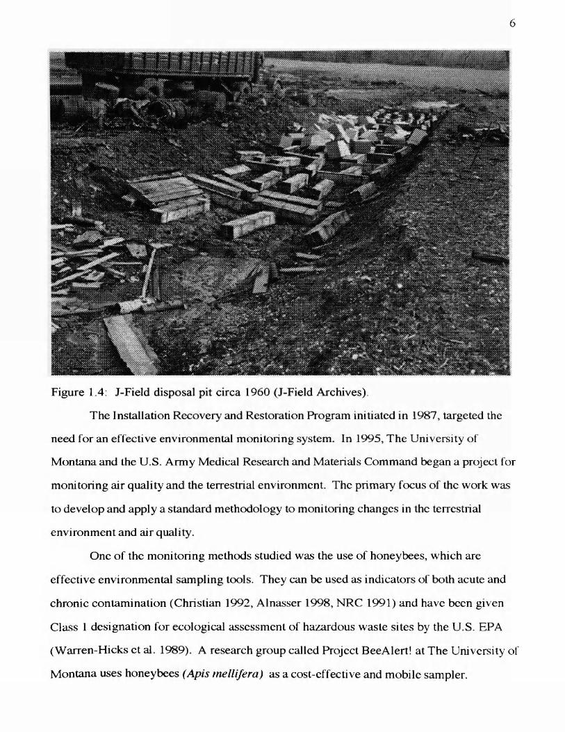
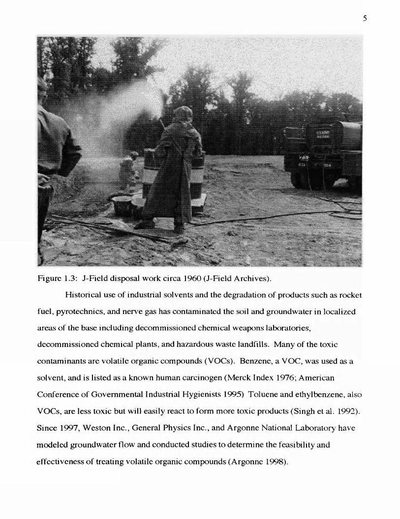
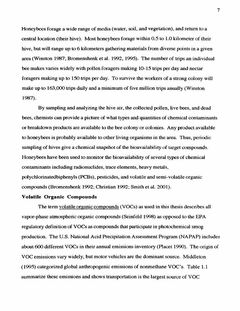
Figure 1.4: J-Field disposal pit circa 1960 (J-Field Archives).
The Installation Recovery and Restoration Program initiated in 1987, targeted the
need for an effective environmental monitoring system. In 1995, The University of
Montana and the U.S. Army Medical Research and Materials Command began a project for
monitoring air quality and the terrestrial environment. The primary focus of the work was
to develop and apply a standard methodology to monitoring changes in the terrestrial
environment and air quality.
One of the monitoring methods studied was the use of honeybees, which are
effective environmental sampling tools. They can be used as indicators of both acute and
chronic contamination (Christian 1992, Alnasser 1998, NRC 1991) and have been given
Class 1 designation for ecological assessment of hazardous waste sites by the U.S. EPA
(Warren-Hicks et al. 1989). A research group called Project BeeAlert! at The University of
Montana uses honeybees (Apis mellifera) as a cost-effective and mobile sampler.
Honeybees forage a wide range of media (water, soil, and vegetation), and return to a
central location (their hive). Most honeybees forage within 0.5 to 1.0 kilometer of their
hive, but will range up to 6 kilometers gathering materials from diverse points in a given
area (Winston 1987; Bromenshenk et al. 1992, 1995). The number of trips an individual
bee makes varies widely with pollen foragers making 10-15 trips per day and nectar
foragers making up to 150 trips per day. To survive the workers of a strong colony will
make up to 163,000 trips daily and a minimum of five million trips anually (Winston
1987).
By sampling and analyzing the hive air, the collected pollen, live bees, and dead
bees, chemists can provide a picture of what types and quantities of chemical contaminants
or breakdown products are available to the bee colony or colonies. Any product available
to honeybees is probably available to other living organisms in the area. Thus, periodic
sampling of hives give a chemical snapshot of the bioavailability of target compounds.
Honeybees have been used to monitor the bioavailability of several types of chemical
contaminants including radionuclides, trace elements, heavy metals,
polychlorinatedbiphenyls (PCBs), pesticides, and volatile and semi-volatile organic
compounds (Bromenshenk 1992; Christian 1992; Smith et al. 2001).
Volatile Organic Compounds
The term volatile organic compounds (VOCs) as used in this thesis describes all
vapor-phase atmospheric organic compounds (Seinfeld 1998) as opposed to the EPA
regulatory definition of VOCs as compounds that participate in photochemical smog
production. The U.S. National Acid Precipitation Assessment Program (NAPAP) includes
about 600 different VOCs in their annual emissions inventory (Placet 1990). The origin of
VOC emissions vary widely, but motor vehicles are the dominant source. Middleton
(1995) categorized global anthropogenic emissions of nonmethane VOC’s. Table 1.1
summarize these emissions and shows transportation is the largest source of VOC
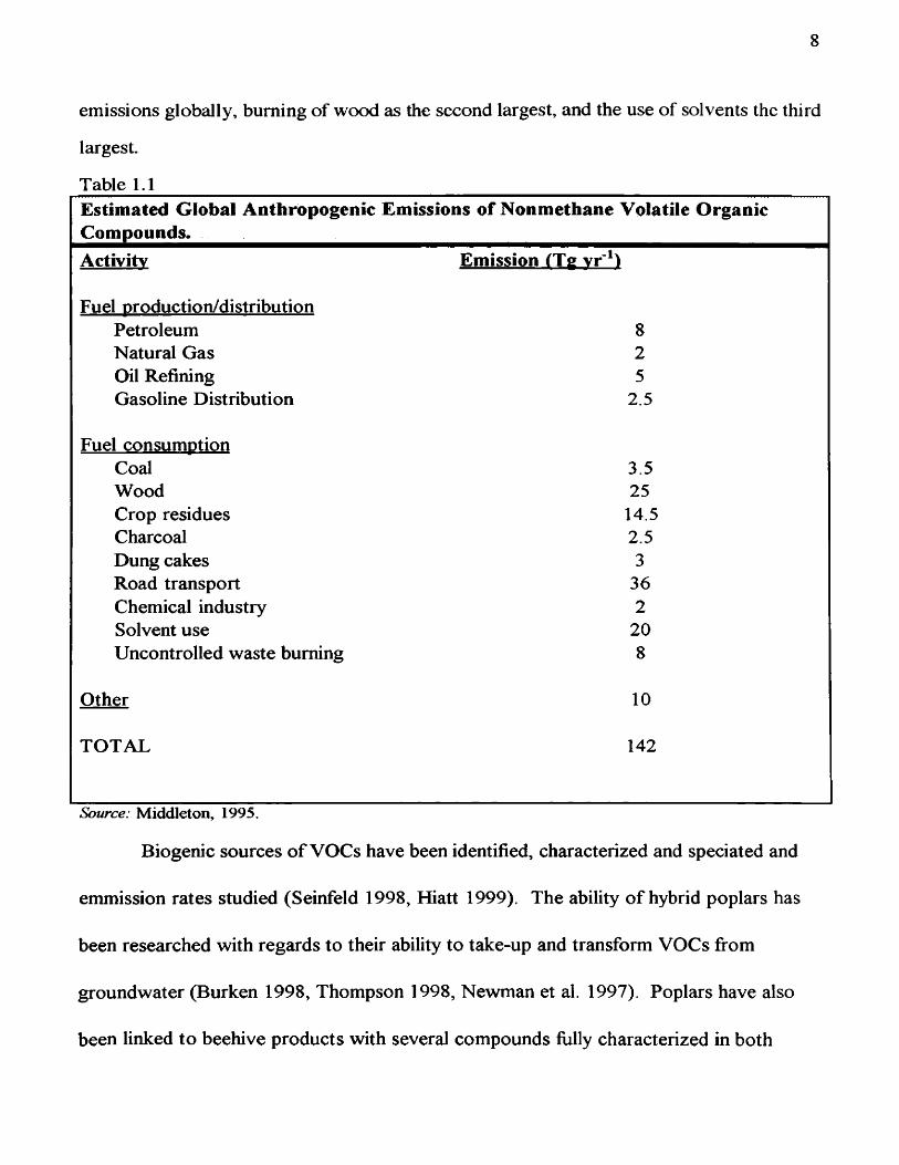
emissions globally, burning of wood as the second largest, and the use of solvents the third
largest.
Table 1.1Estimated Global Anthropogenic Emissions of Nonmethane Volatile Organic Compounds.Activity Emission tXç vr^l
Fuel production/distributionPetroleum 8Natural Gas 2Oil Refining 5Gasoline Distribution 2.5
Fuel consumptionCoal 3.5Wood 25Crop residues 14.5Charcoal 2.5Dung cakes 3Road transport 36Chemical industry 2Solvent use 20Uncontrolled waste burning 8
Other 10
TOTAL 142
Source: M iddleton, 1995.
Biogenic sources o f VOCs have been identified, characterized and speciated and
emmission rates studied (Seinfeld 1998, Hiatt 1999). The ability o f hybrid poplars has
been researched with regards to their ability to take-up and transform VOCs from
groundwater (Burken 1998, Thompson 1998, Newman et al. 1997). Poplars have also
been linked to beehive products with several compounds fully characterized in both
poplar buds and beehive propolis (Bankova 1982, 1989; Martos 1997). More than 100
VOCs, some related to poplar buds and propolis, have been identified in beehive
atmospheres (Smith et al. 2001).
STATEMENT OF PROBLEM
APG has a lengthy history of toxic chemical use and is adjacent to a highly
populated urban and suburban area The U.S. Environmental Protection Agency added
the Edgewood Area to National Priorities List in February 1990 because of the potential
impact o f the toxic chemicals on the surrounding community. Project BeeAlert!
investigated this potential impact beginning in 1995 and has shown that certain areas of
APG have high levels o f bioavailable contaminants. Further, BeeAlert! has shown
significant reductions of bioavailable contaminants at sites where the Installation
Recovery and Restoration Program work has taken place (Bromenshenk et al. 1997; 1998).
The purpose of this study is to determine if APG is a source of regionally
distributed bioavailable volatile organic chemicals and if these contaminants are dispersed
into adjacent communities from the proving ground as a function o f distance and/or
direction.
Project BeeAlert! initiated a boundary study in 1998 to specifically determine
whether the proving ground was a source of contamination to the surrounding area. In
1998, the team surveyed the area to determine what types and concentrations of compounds
the honeybees were collecting. I utilized 1998 survey information, upgraded
instrumentation, and fine-tuned methodology to implement a comprehensive study in 1999.
10
THESIS ORGANIZATION
The remainder of this thesis is organized into three additional chapters. In
Chapter 2 I detail the experimental methods including the deployment of beehives, sample
collection technique, sample analysis protocols, and quality assurance measures taken. I
present the study results in Chapter 3, including the data reduction techniques for both
years and an analysis o f variance of the 1999 data. The discussion, conclusions and
suggestions for further study appear in Chapter 4.
CHAPTER 2: EXPERIMENTAL METHOD
O verview
To determine whether or not APG is a source of regionally distributed bioavailable
VOCs, the boundary study was conducted in two phases. The first phase, performed from
June through October 1998, identified bioavailable compounds and concentrations in the
hives and ambient air. The second phase of the project, accomplished from June through
September 1999, quantified compounds identified in 1998, quantified additional
compounds, and identified patterns in seasonal variation and spatial distribution.
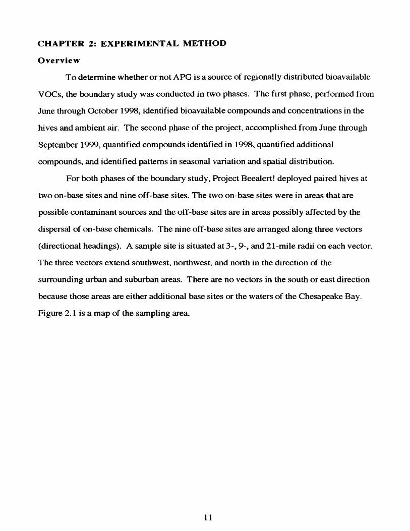
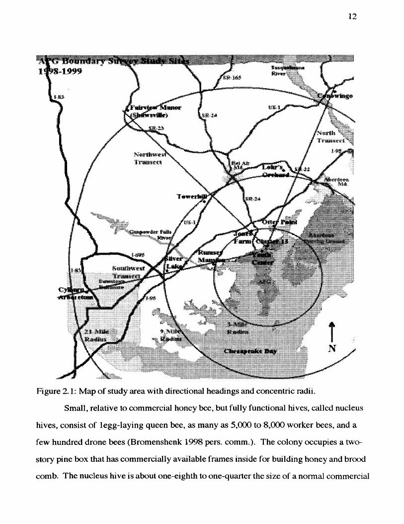
For both phases of the boundary study. Project Beealert! deployed paired hives at
two on-base sites and nine off-base sites. The two on-base sites were in areas that are
possible contaminant sources and the off-base sites are in areas possibly affected by the
dispersal of on-base chemicals. The nine off-base sites are arranged along three vectors
(directional headings). A sample site is situated at 3-, 9-, and 21-mile radii on each vector.
The three vectors extend southwest, northwest, and north in the direction of the
surrounding urban and suburban areas. There are no vectors in the south or east direction
because those areas are either additional base sites or the waters of the Chesapeake Bay.
Figure 2.1 is a map of the sampling area.
11
12
fUi' /.
Figure 2.1: Map of study area with directional headings and concentric radii.
Small, relative to commercial honey bee, but fully functional hives, called nucleus
hives, consist of 1 egg-laying queen bee, as many as 5,000 to 8,000 worker bees, and a
few hundred drone bees (Bromenshenk 1998 pers. comm.). The colony occupies a two-
story pine box that has commercially available frames inside for building honey and brood
comb. The nucleus hive is about one-eighth to one-quarter the size of a normal commercial
13
beehive used for honey production and, because of its small size, is easily moved and
relatively inconspicuous when deployed.
The hive air and ambient air were sampled periodically using as guidelines the U.S.
EPA’s Compendium Method TO-17: Determination of Volatile Organic Compounds in
Ambient Air Using Active Sampling Onto Sorbents Beds. The samples were then analyzed
using Thermal Desorbtion/Gas Chromatography/Mass Spectrometry (TD/GC/MS). This is
a widely accepted method of VOC monitoring (Russel 1975; Woolfenden 1997; Wrobel
2000).
Sample collection
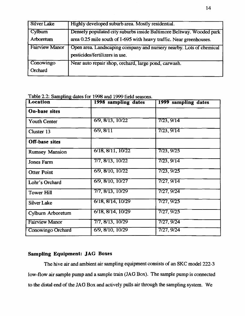
Each site was sampled every six to eight weeks during summer and early fall of
1998 and 1999. Samples of the air within the hive (hive air) and of the air outside the hive
(ambient air) were collected. The sampling sites represent a diverse range of human
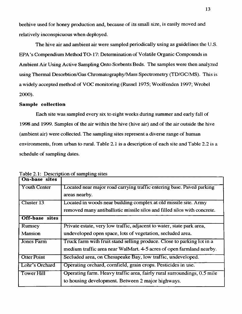
environments, from urban to rural. Table 2.1 is a description of each site and Table 2.2 is a
schedule of sampling dates.
Table 2.1: Description of sampling sitesOn-base sitesY outh Center Located near major road carrying traffic entering base. Paved parking
areas nearby.Cluster 13 Located in woods near building complex at old missile site. Army
removed many antiballistic missile silos and filled silos with concrete.Off-base sitesRumseyMansion
Private estate, very low traffic, adjacent to water, state park area, undeveloped open space, lots of vegetation, secluded area.
Jones Farm Truck farm with fruit stand selling produce. Close to parking lot in a medium traffic area near WalMart. 4-5 acres of open farmland nearby.
Otter Point Secluded area, on Chesapeake Bay, low traffic, undeveloped.Lohr’s Orchard Operating orchard, cornfield, grain crops. Pesticides in use.Tower Hill Operating farm. Heavy traffic area, fairly rural surroundings, 0.5 mile
to housing development. Between 2 major highways.
14
Silver Lake Highly developed suburb area. Mostly residential.CylbumArboretum
Densely populated city suburbs inside Baltimore Beltway. Wooded park area 0.25 mile south of 1-695 with heavy traffic. Near greenhouses.
Fairview Manor Open area. Landscaping company and nursery nearby. Lots of chemical pesticides/fertilizers in use.
ConowingoOrchard
Near auto repair shop, orchard, large pond, carwash.
Table 2.2: Sampling dates for 1998 and 1999 field seasonsLocation 1998 sampling dates 1999 sampling dates
On-base sites
Youth Center 6/9, 8/13, 10/22 7/23, 9/14
Cluster 13 6/9, 8/11 7/23, 9/14
Off-base sites
Rumsey Mansion 6/18,8/11, 10/22 7/23, 9/25
Jones Farm 7/7, 8/13, 10/22 7/23, 9/14
Otter Point 6/9, 8/10, 10/22 7/23, 9/25
Lohr’s Orchard 6/9, 8/10, 10/27 7/27, 9/14
Tower Hill 7/7, 8/13, 10/29 7/27, 9/24
Silver Lake 6/18, 8/14, 10/29 7/27,9/25
Cylbum Arboretum 6/18, 8/14, 10/29 7/27, 9/25
Fairview Manor 7/7, 8/13, 10/29 7/27, 9/24Conowingo Orchard 6/9, 8/10, 10/29 7/27, 9/24
Sampling Equipment: JAG Boxes
The hive air and ambient air sampling equipment consists of an SKC model 222-3
low-flow air sample pump and a sample train (JAG Box). The sample pump is connected
to the distal end of the JAG Box and actively pulls air through the sampling system. We
15
specifically designed the JAG Box for sampling the atmosphere of a beehive, which
requires certain considerations beyond normal air sampling. First, hives are extremely
humid. Worker bees collect water from standing water sources and use the water along
with wing fanning to cool the hive. High humidity in the hive air samples can destroy the
sample so water removal is the first priority. Second, hive atmospheres are chemically rich
environments. Large molecules such as terpenes and carbohydrates that are present in
hives act as chemical interferents in subsequent TD/GC/MS analysis. An organic varnish
accumulates on the inside of the transfer lines and leads to substantial chemical carry-over
from sample to sample. The heavy compounds overwhelm the trace levels of the target
analytes so removal of them before analysis is the second priority.
The JAG Box consists of three tubes connected in-line with brass Swagelok fittings
and 1/8-inch copper tubing housed in a 710-mL Rubbermaid "servin' saver." The
Rubbermaid servin' saver is a weatherproof housing for the sample tubes. The copper
tubing and Swagelok fittings run through three holes drilled in the short ends of the
"servin' saver". At the proximal end is a piece of 8-inch x 1/8-inch copper tubing that is
either inserted into the hive or left out of the hive for an ambient air sample. Moving
distally, an SKC model 226-44-02 drying tube packed with 9000 mg of anhydrous sodium
sulfate is attached to the insertion tube. Water molecules are sorbed to the sodium sulfate
as air is pulled through the tube. Next is a Supelco Carbotrap 150, which acts as a guard-
tube to remove the larger sugar and carbohydrate molecules not of interest in analysis. The
third tube in the sample train, the tube that collects the sample, is a Supelco Carbotrap 400.
To sample the hive air, a 5/32-inch hole is drilled into the wall of the hive so that the
sampling tube from the JAG box can be inserted between the frames in the hive.
The Carbotrap 150 and 400 are 11.5 cm x 6 mm OD x 4mm ID thermal desorbtion
tubes. The Carbotrap 150 is packed with 300 mg 20/40 mesh Carbotrap C graphitized
carbon black material with a surface area of 12 m^/gram, is highly effective at absorbing
and releasing high molecular weight airborne contaminants (C9 to C30) while allowing the
16
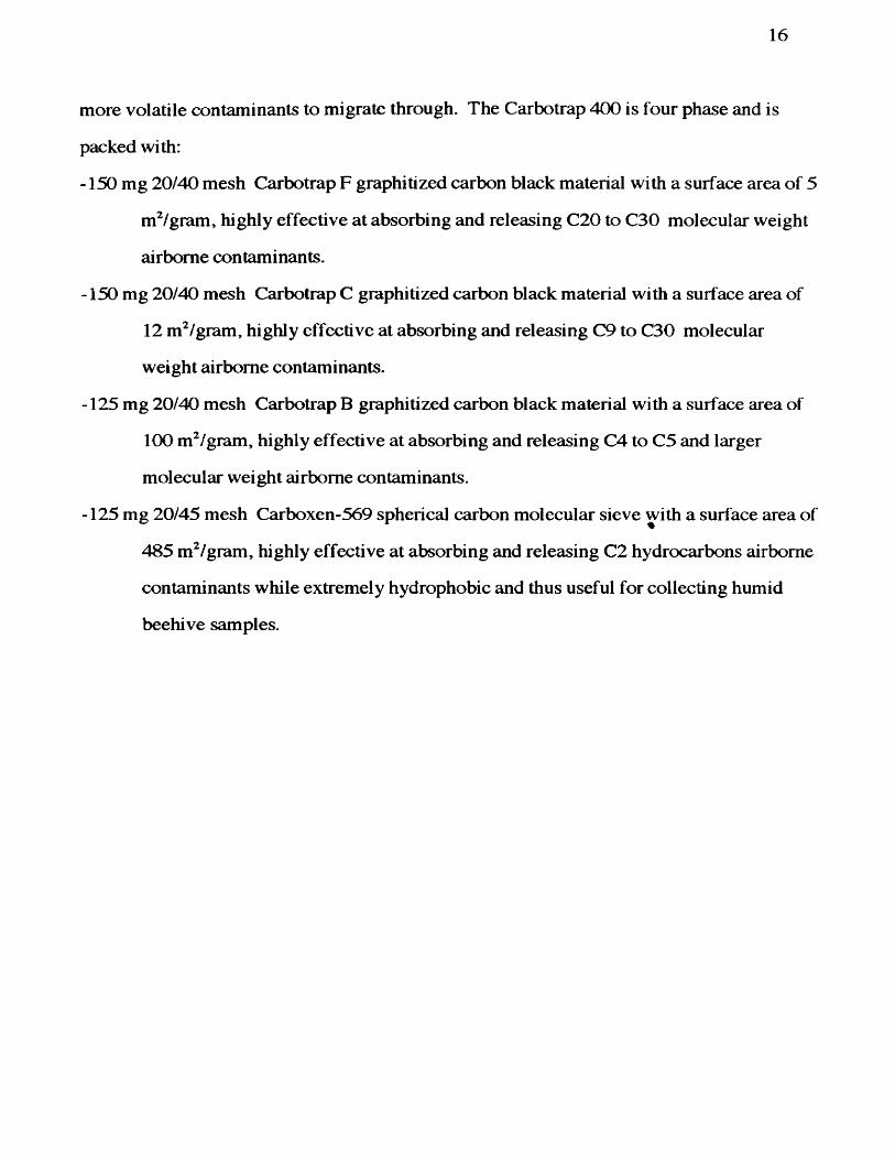
more volatile contaminants to migrate through. The Carbotrap 400 is four phase and is
packed with:
-150 mg 20/40 mesh Carbotrap F graphitized carbon black material with a surface area of 5
m^/gram, highly effective at absorbing and releasing C20 to C30 molecular weight
airborne contaminants.
-150 mg 20/40 mesh Carbotrap C graphitized carbon black material with a surface area of
12 m^/gram, highly effective at absorbing and releasing C9 to C30 molecular
weight airborne contaminants.
-125 mg 20/40 mesh Carbotrap B graphitized carbon black material with a surface area of
100 m^/gram, highly effective at absorbing and releasing C4 to C5 and larger
molecular weight airborne contaminants.
-125 mg 20/45 mesh Carboxen-569 spherical carbon molecular sieve with a surface area of
485 m^/gram, highly effective at absorbing and releasing C2 hydrocarbons airborne
contamincints while extremely hydrophobic and thus useful for collecting humid
beehive samples.
17
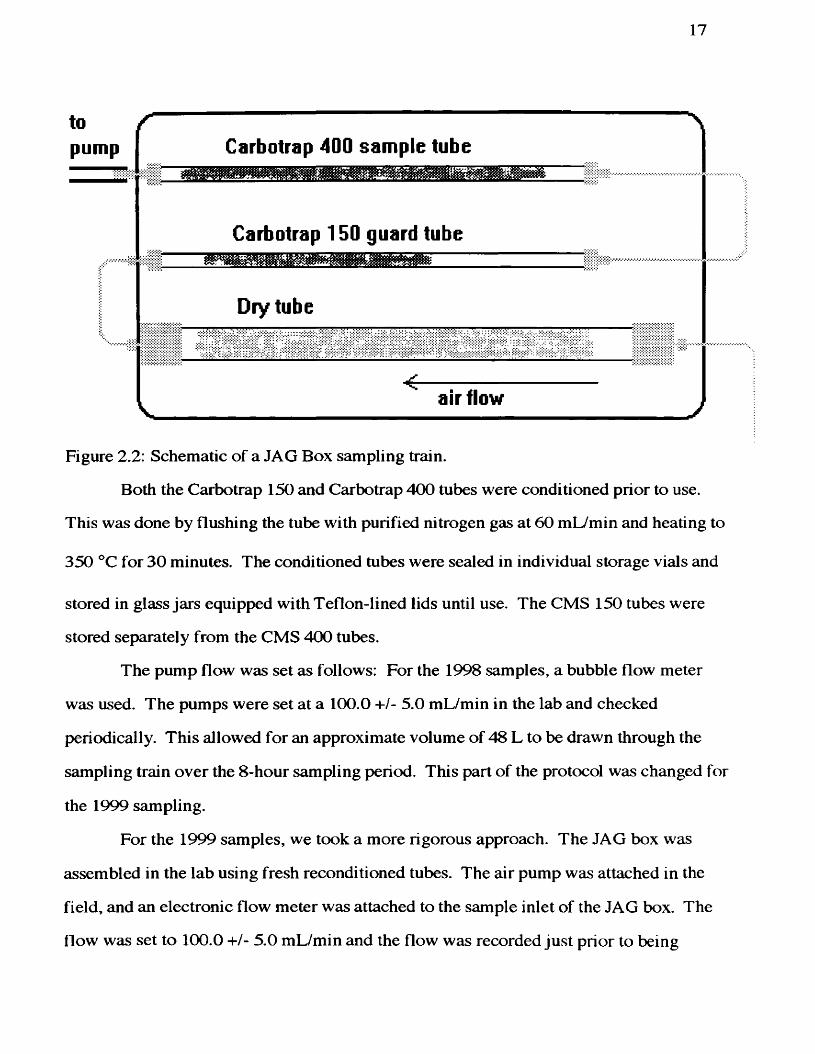
to rpump Carbotrap 400 sam ple tube
Carbotrap 150 guard tube
Dry tube
air flow
Figure 2.2: Schematic of a JAG Box sampling train.
Both the Carbotrap 150 and Carbotrap 400 tubes were conditioned prior to use.
This was done by flushing the tube with purified nitrogen gas at 60 mL/min and heating to
350 * C for 30 minutes. The conditioned tubes were sealed in individual storage vials and
stored in glass jars equipped with Teflon-lined lids until use. The CMS 150 tubes were
stored separately from the CMS 400 tubes.
The pump flow was set as follows: For the 1998 samples, a bubble flow meter
was used. The pumps were set at a 100.0 +/- 5.0 mL/min in the lab and checked
periodically. This allowed for an approximate volume of 48 L to be drawn through the
sampling train over the 8-hour sampling period. This part of the protocol was changed for
the 1999 sampling.
For the 1999 samples, we took a more rigorous approach. The JAG box was
assembled in the lab using fresh reconditioned tubes. The air pump was attached in the
field, and an electronic flow meter was attached to the sample inlet of the JAG box. The
flow was set to 100.0 +/- 5.0 mL/min and the flow was recorded just prior to being
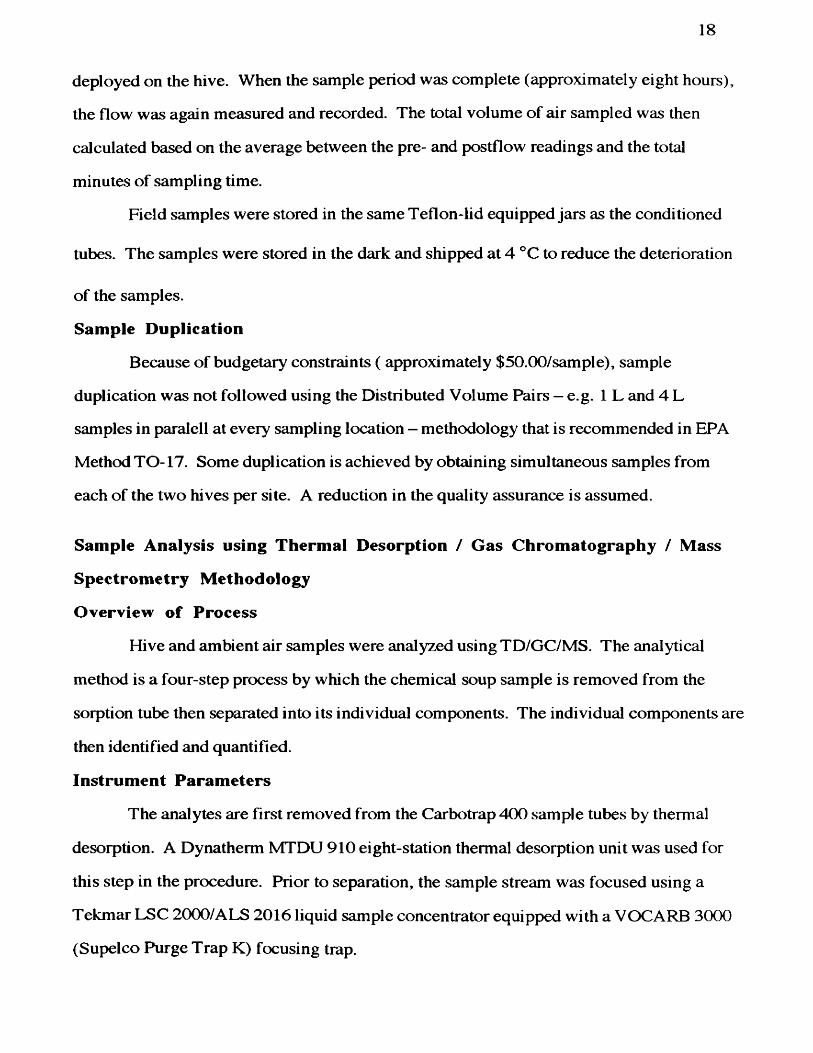
18
deployed on the hive. When the sample period was complete (approximately eight hours),
the flow was again measured and recorded. The total volume of air sampled was then
calculated based on the average between the pre- and postflow readings and the total
minutes of sampling time.
Field samples were stored in the same Teflon-lid equipped jars as the conditioned
tubes. The samples were stored in the dark and shipped at 4 to reduce the deterioration
of the samples.
Sample Duplication
Because of budgetary constraints ( approximately $50.00/sample), sample
duplication was not followed using the Distributed Volume Pairs — e.g. 1 L and 4 L
samples in paralell at every sampling location - methodology that is recommended in EPA
Method TO-17. Some duplication is achieved by obtaining simultaneous samples from
each of the two hives per site. A reduction in the quality assurance is assumed.
Sample Analysis using Thermal Desorption / Gas Chromatography / Mass
Spectrometry Methodology
Overview o f Process
Hive and ambient air samples were analyzed using TD/GC/MS. The analytical
method is a four-step process by which the chemical soup sample is removed from the
sorption tube then separated into its individual components. The individual components are
then identified and quantified.
Instrument Parameters
The analytes are first removed from the Carbotrap 400 sample tubes by thermal
desorption. A Dynatherm MTDU 910 eight-station thermal desorption unit was used for
this step in the procedure. Prior to separation, the sample stream was focused using a
Tekmar LSC 2000/ALS 2016 liquid sample concentrator equipped with a VOCARB 3000
(Supelco Purge Trap K) focusing trap.
19
The analytes were separated using a Hewlett Packard 5890 series II gas
chromatograph equipped with a Restek RTX 502.2 capillary column. Once separated, the
analytes were introduced into a Hewlett Packard 5971 electron ionization mass
spectrometer. Identification and quantification were carried out using Hewlett Packard
Enviroquant computer software.
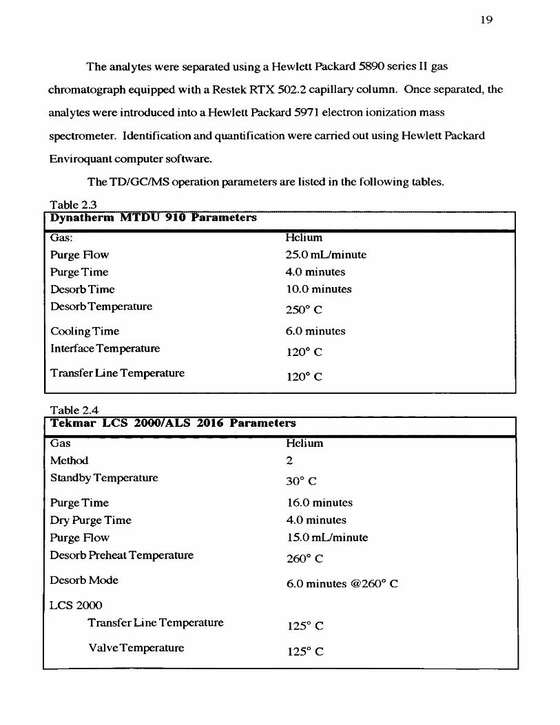
The TD/GC/MS operation parameters are listed in the following tables.
Table 2.3Dynatherm MTDU 910 Parameters
Gas: HeliumPurge How 25.0 mL/minutePurge Time 4.0 minutesDesorb Time 10.0 minutesDesorb T emperature 250^ C
Cooling Time 6.0 minutesInterface Temperature 120° C
T ransfer Line T emperature 120° C
Table 2.4Tekmar LCS 2000/ALS 2016 Parameters
Gas HeliumMethod 2Standby Temperature 30° C
Purge Time 16.0 minutesDry Purge Time 4.0 minutesPurge How 15.0 mL/minuteDesorb Preheat Temperature 260° C
Desorb Mode 6.0 minutes @260° C
LCS 2000Transfer Line Temperature 125° C
Valve T emperature 125° C
20
ALS 2016T ransfer Line Temperature 120° C
Valve T emperature 120° C
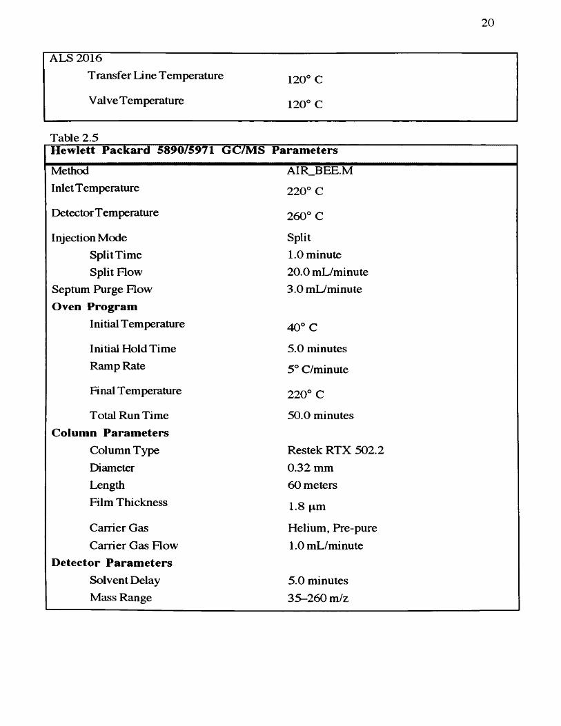
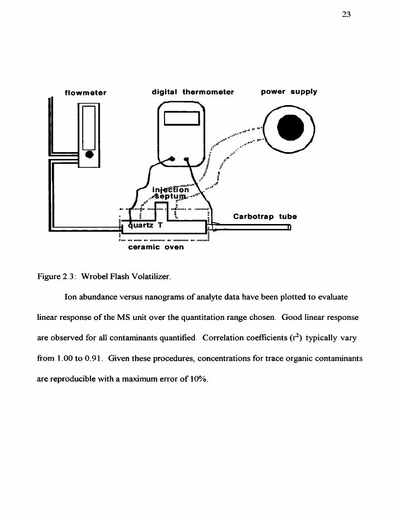
Table 2.5Hewlett Packard 5890/5971 GC/MS Parameters
Method a ir _b e e .mInlet T emperature 220° C
Detector T emperature 260° C
Injection Mode SplitSplit Time 1.0 minuteSplit Flow 20.0 mL/minute
Septum Purge Flow 3.0 mL/minuteOven Program
Initial Temperature 40° C
Initial Hold Time 5.0 minutesRamp Rate 5° C/minute
Final Temperature 220° C
Total Run Time 50.0 minutesColumn Parameters
Column Type Restek RTX 502.2Diameter 0.32 mmLength 60 metersFilm Thickness 1.8 pm
Carrier Gas Helium, Pre-pureCarrier Gas Row 1.0 mL/minute
Detector ParametersSolvent Delay 5.0 minutesMass Range 35-260 m/z
21
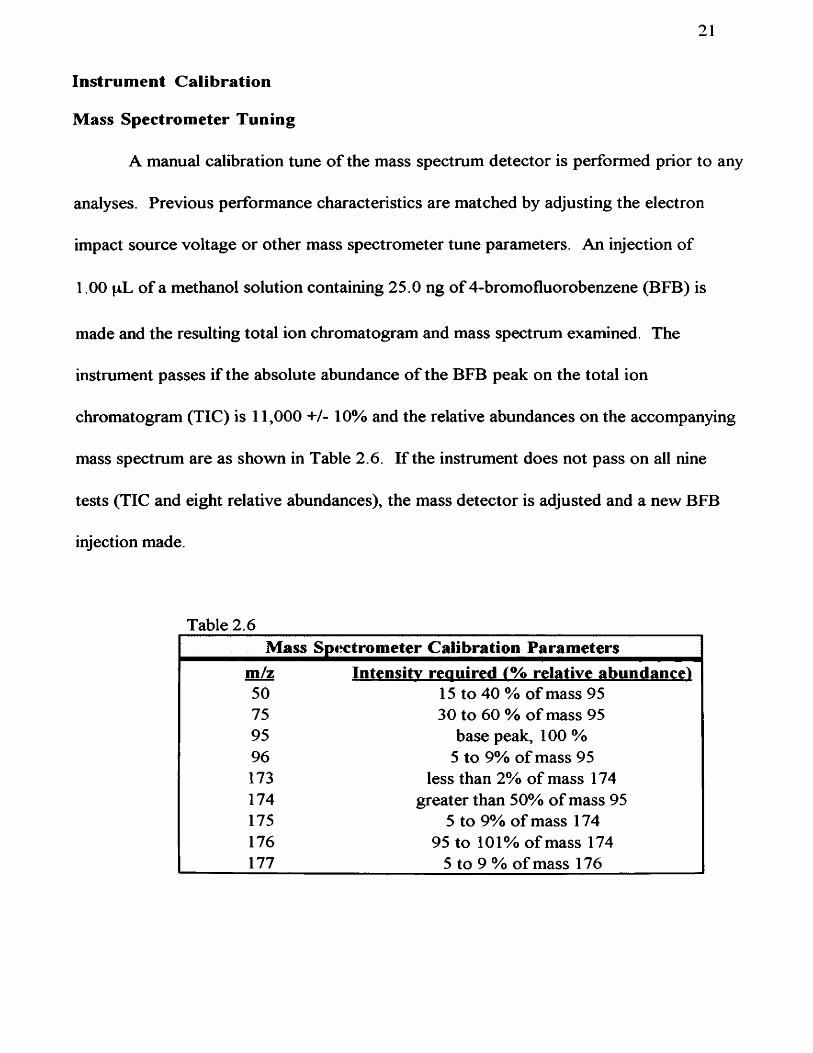
Instrument Calibration
Mass Spectrometer Tuning
A manual calibration tune of the mass spectrum detector is performed prior to any
analyses. Previous performance characteristics are matched by adjusting the electron
impact source voltage or other mass spectrometer tune parameters. An injection of
1.00 pL of a methanol solution containing 25.0 ng of 4-bromofluorobenzene (BFB) is
made and the resulting total ion chromatogram and mass spectrum examined. The
instrument passes if the absolute abundance of the BFB peak on the total ion
chromatogram (TIC) is 11,000 +/- 10% and the relative abundances on the accompanying
mass spectrum are as shown in Table 2 .6. If the instrument does not pass on all nine
tests (TIC and eight relative abundances), the mass detector is adjusted and a new BFB
injection made.
Table 2.6Mass Sp«^ctrometer Calibration Parameters
m/z Intensity required t% relative abundance!50 15 to 40 % of mass 9575 30 to 60 % of mass 9595 base peak, 100 %96 5 to 9% of mass 95173 less than 2% of mass 174174 greater than 50% of mass 95175 5 to 9% of mass 174176 95 to 101% of mass 174177 5 to 9 % of mass 176
22
Internal Standard
Every sample tube is dosed with 1.00 pL of an internal standard solution prior to
TD/GC/MS analysis so that the efficiency o f the desorption and transfer of material from
the tube into the GC can be assured. The internal standard consists of 100 ng
fluorobenzene (Supelco, 4-8948). Also added as surrogates, are 100 ng each of
4-bromofluorobenzene and l,2-d4-dichlorobenzene (Supelco, 4-8083). The two surrogate
compounds serve as a quantity check for target analytes.
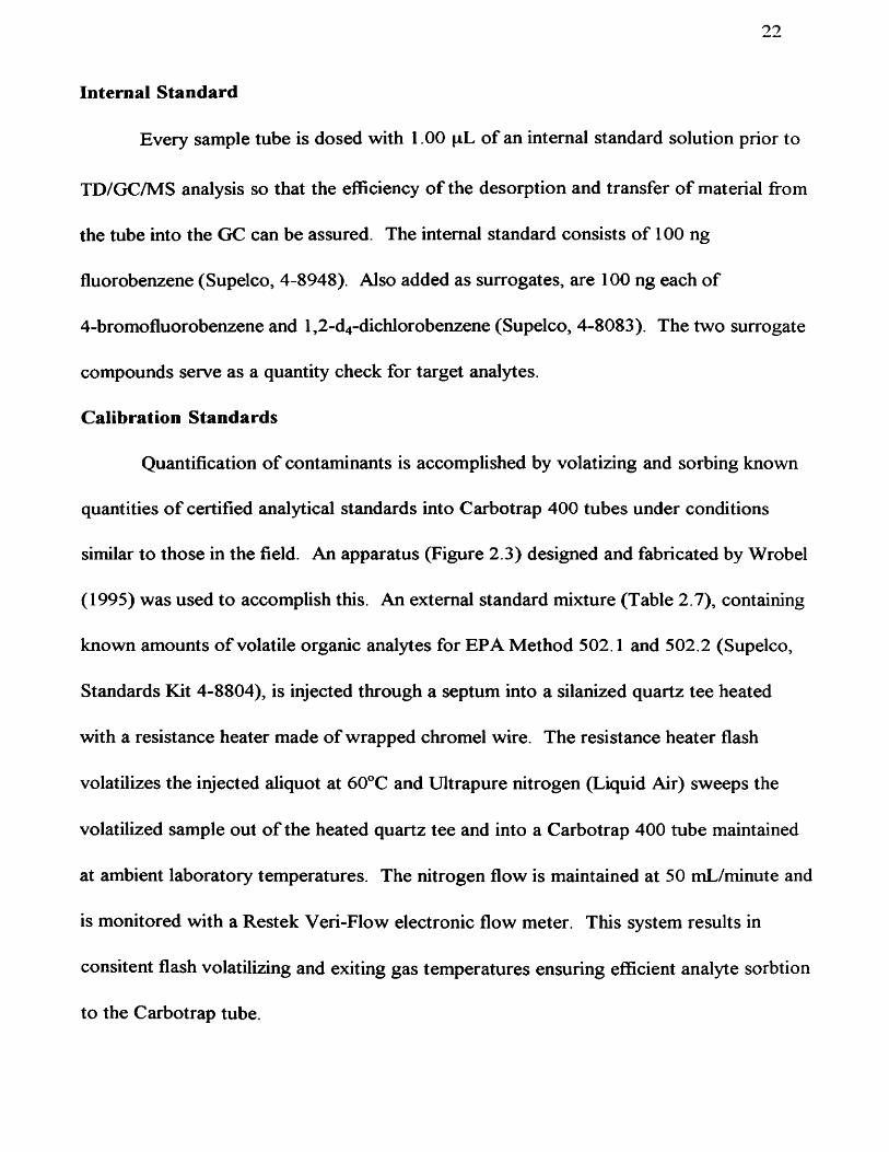
Calibration Standards
Quantification o f contaminants is accomplished by volatizing and sorbing known
quantities of certified analytical standards into Carbotrap 400 tubes under conditions
similar to those in the field. An apparatus (Figure 2.3) designed and fabricated by Wrobel
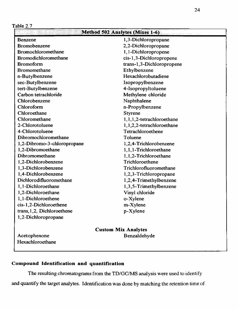
(1995) was used to accomplish this. An external standard mixture (Table 2.7), containing
known amounts o f volatile organic analytes for EPA Method 502.1 and 502.2 (Supelco,
Standards Kit 4-8804), is injected through a septum into a silanized quartz tee heated
with a resistance heater made of wrapped chromel wire. The resistance heater flash
volatilizes the injected aliquot at 60°C and Ultrapure nitrogen (Liquid Air) sweeps the
volatilized sample out o f the heated quartz tee and into a Carbotrap 400 tube maintained
at ambient laboratory temperatures. The nitrogen flow is maintained at 50 mL/minute and
is monitored with a Restek Veri-Flow electronic flow meter. This system results in
consitent flash volatilizing and exiting gas temperatures ensuring efficient analyte sorbtion
to the Carbotrap tube.
23
flowmeter digital thermometer
/ N
power supply
-// /
inj«£{ron“
!***•«• •« ■*•••••»**
,4 e p tu ^ .n •
* # « ( I ' « f i. J li ,w quartz T I
Carbotrap tube
########## ## ########## ##
ceramic oven
Figure 2.3 : Wrobel Flash Volatilizer.
Ion abundance versus nanograms of analyte data have been plotted to evaluate
linear response of the MS unit over the quantitation range chosen. Good linear response
are observed for all contaminants quantified. Correlation coefficients (r^) typically vary
from 1.00 to 0.91. Given these procedures, concentrations for trace organic contaminants
are reproducible with a maximum error o f 10%.
24
Table 2.7.....
Benzene 1,3 -DichloropropaneBromobenzene 2,2-DichloropropaneBromochloromethane 1,1 -DichloropropeneBromodichloromethane cis-1,3 -DichloropropeneBromoform trans-1,3 -DichloropropeneBromomethane Ethylbenzenen-Butylbenzene Hexachlorobutadienesec-Butylbenzene Isopropylbenzenetert-Butylbenzene 4-IsopropyltolueneCarbon tetrachloride Methylene chlorideChlorobenzene NaphthaleneChloroform n-PropylbenzeneChloroethane StyreneChloromethane 1,1,1,2-tetrachloroethane2-Chlorotoluene 1,1,2,2-tetrachloroethane4-Chlorotoluene T etrachloroetheneDibromochloromethane Toluene1,2-Dibromo-3-chloropropane 1,2,4-T richlorobenzene1,2-Dibromoethane 1,1,1-T richloroethaneDibromomethane 1,1,2-T richloroethane1,2-Dichlorobenzene T richloroethene1,3 -Dichlorobenzene T richlorofluor omethane1,4-Di chlorobenzene 1,2,3-T richloropropaneDichlorodifluoromethane 1,2,4-Trimethylbenzene1,1 -Dichloroethane 1,3,5-T r imet hylbenzene1,2-Dichloroethane Vinyl chloride1,1 -Dichloroethene o-Xylenecis-1,2-Dichloroethene m-Xylenetrans, 1,2, Dichloroethene p-Xylene1,2-Dichloropropane
Custom Mix AnalytesAcetophenone BenzaldehydeHexachloroethane
Compound Identification and quantification
The resulting chromatograms from the TD/GC/MS analysis were used to identify
and quantify the target analytes. Identification was done by matching the retention time of
25
the sample analyte with the retention time of the standard analyte. When the correct peak
was identified, the compound was verified by matching the mass spectrum of the sample
analyte with a National Institute of Science and Technology (NIST) mass spectral library.
Quantification of the target analytes was carried out using two different strategies
for the two years of analysis. For the 1998 samples, a response factor (RF) for each of the
target analytes was calculated (equation 2.1) by comparing the peak area of a known
amount of the target analyte with the peak area of the internal standard (Harris 1995):
(2 . 1)Ais • Mt
where :
At = area of target analyte A is = area of internal standard M t = mass of target analyte Mis = mass of internal standard
The quantity of each compound in each sample was then calculated (equation 2.2) using the
maximum abundance of the molecular ion instead of the peak area of the target analyte.
This was done because in some cases when trace quantities were analyzed, the peak area of
the target analyte was difficult to integrate and often coelluted with other non target analytes
that are part of the normal hive chemistry.
Q - ^where :
Qt = quantity of target analyte in ng.RF = response factor for target analyte
For the 1999 samples, we were interested in expanding the number of target
analytes and achieving a higher level of QA/QC than what was attained in the 1998 samples
and. A quantitation database was established using a six-point calibration curve for each of
55 compounds. Standards of concentrations 5.00, 25.0, 50.0, 100, 200, and 400 ng/pL
26
were made from 2000 ng/^iL certified stock solutions and and used for the calibration
curves. Once calibration curves are established (r = .991 to 1.00), quantitation is made
using the Hewlett-Packard Enviroquant software.
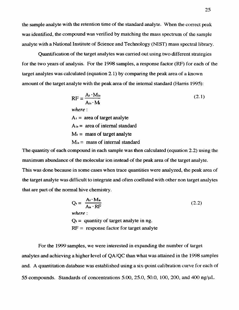
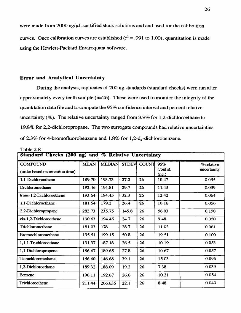
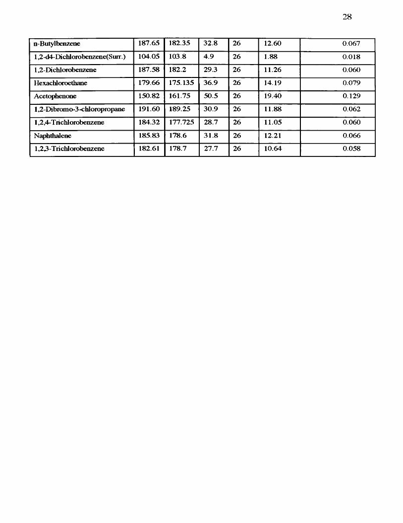
Error and Analytical Uncertainty
During the analysis, replicates of 200 ng standards (standard checks) were run after
approximately every tenth sample (n=26). These were used to monitor the integrity of the
quantitation data file and to compute the 95% confidence interval and percent relative
uncertainty (%). The relative uncertainty ranged from 3.9% for 1,2-dichloroethane to
19.8% for 2,2-dichloropropane. The two surrogate compounds had relative uncertainties
of 2.3% for 4-bromofluorobenzene and 1.8% for 1,2-d^-dichlorobenzene.
Table 2.8Standard Checks (200 ng) and % Relative Uncertainty
COMPOUND
(order based on retention time)
MEAN MEDIAN STDEV COUNT 95%Confid.(ng.)
% relative uncertainty
1,1 -Dichloroethene 189.70 193.73 27.2 26 10.47 0.055
Dichloromethane 192.46 194.81 29.7 26 11.43 0.059
trans-1,2-Dichloroethene 193.64 194.45 32.3 26 12.42 0.064
1,1 -Dichloroethane 181.54 179.2 26.4 26 10.16 0.056
2,2 Dichloropropane 282.73 235.75 145.8 26 56.03 0.198
cis 1,2-Dichloroethene 190.63 194.45 24.7 26 9.48 0.050
T richloromethane 181.03 178 28.7 26 11.02 0.061
Bromochloromethane 195.51 199.15 50.8 26 19.51 0.100
1,1,1 Tiichloroethane 191.97 187.18 26.5 26 10.19 0.053
1,1 Dichloropropene 186.67 189.65 27.8 26 10.67 0.057
Tetrachloromethane 156.60 146.68 39.1 26 15.03 0.096
1,2 Dichloroethane 189.32 188.09 19.2 26 7.38 0.039
Benzene 190.11 192.67 26.6 26 10.21 0.054
Trichloroethene 211.44 206.635 22.1 26 8.48 0.040
27
1,2-Dichloropropane 168.44 180.3 46.9 26 18.03 0.107
BromodichlQromethaiie 170.53 178.95 49.0 26 18.83 0.110
Dibromomethane 205.15 199 26.8 26 10.32 0.050
13-Dichloro- 1-propene 178.81 188.2 44.0 26 16.90 0.095
Toluene 207.15 205.25 38.2 26 14.68 0.071
trans 13 Dichlom- 1-propene 174.35 183.55 50.7 26 19.48 0.112
1,1,2-TrichloroeÜiane 176.88 191.96 42.7 26 16.42 0.093
13-Dichloiopropane 179.90 187.415 39.8 26 15.31 0.085
Tetmdiloroethene 202.58 201.95 24.1 26 9.25 0.046
Dibromochloromethane 156.58 181.68 60.7 26 23.35 0.149
1,2-Dibromoethane 171.76 196.45 56.1 26 21.56 0.126
Chlorobenzene 198.90 202.75 23.5 26 9.03 0.045
1,1,13-Tetrachloroethane 185.08 184.3 34.1 26 13.10 0.071
Ethylbenzene 197.38 200.8 31.7 26 12.18 0.062
m,p Xylenes 407.03 401.45 51.3 26 19.73 0.048
o-Xylene 198.71 199.65 23.5 26 9.02 0.045
Styrene (Ethenylbenzene) 195.55 196.35 23.9 26 9.18 0.047
Isopropylbenzene 201.73 198.14 25.0 26 9.60 0.048
T ribromomethane 144.98 171.35 65.3 26 25.10 0.173
1,1,23-Tetrachloroethane 160.91 165.76 47.8 26 18.39 0.114
1 -Bromo-4-fluorobenzene(SuiT.) 97.70 96.76 5.9 26 2.28 0.023
1,23-Tiichloropropane 160.33 166.35 49.3 26 18.94 0.118
n-Propylbenzene 198.94 195.9 25.2 26 9.70 0.049
Bromobenzene 190.46 193.05 31.1 26 11.95 0.063
13»5-Trimethyl\benzene 192.99 191.54 29.5 26 11.34 0.059
2-Chlorotoluaie 190.90 188.385 25.2 26 9.69 0.051
4-Chlorotoluene 191.72 191.85 24.8 26 9.54 0.050
tert-Butylbenzene 192.19 186.7 27.7 26 10.65 0.055
1,2,4-T limethylbenzene 189.81 183.55 24.0 26 9.22 0.049
Benzaldehyde 206.62 198.1 60.1 26 23.11 0.112
sec-Butylbenzene 192.87 186.95 28.4 26 10.93 0.057
Isopropyltoluene 188.45 181.75 29.7 26 11.40 0.060
13 -Dichlorobenzene 188.25 186.04 28.2 26 10.85 0.058
1,4-Dichlorobenzene 188.68 187.65 28.1 26 10.80 0.057
28
n-Butylbenzene 187.65 182.35 32.8 26 12.60 0.067
1 -d4-Dichlorobenzene(Siirr.) 104.05 103.8 4.9 26 1.88 0.018
1,2 Dichlorobenzene 187.58 182.2 29.3 26 11.26 0.060
Hexachloroethane 179.66 175.135 36.9 26 14.19 0.079
Acetophenone 150.82 161.75 50.5 26 19.40 0.129
1,2 Dibromo-3 -chloropropane 191.60 189.25 30.9 26 11.88 0.062
1,2,4-Trichlorobenzene 184.32 177.725 28.7 26 11.05 0.060
Na^Ékthalene 185.83 178.6 31.8 26 12.21 0.066
1,23-Trichlorobenzene 182.61 178.7 27.7 26 10.64 0.058
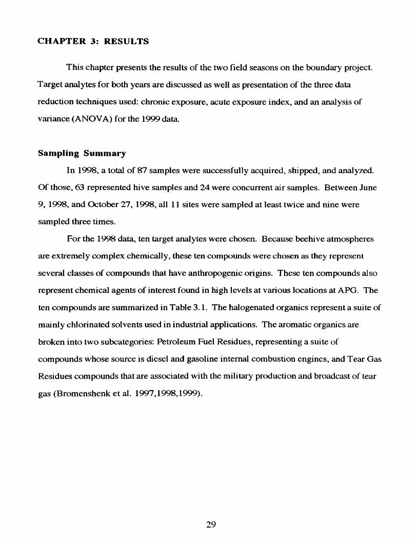
CHAPTER 3: RESULTS
This chapter presents the results of the two field seasons on the boundary project.
Target analytes for both years are discussed as well as presentation of the three data
reduction techniques used: chronic exposure, acute exposure index, and an analysis of
variance (ANOVA) for the 1999 data.
Sampling Summary
In 1998, a total of 87 samples were successfully acquired, shipped, and analyzed.
Of those, 63 represented hive samples and 24 were concurrent air samples. Between June
9, 1998, and October 27, 1998, all 11 sites were sampled at least twice and nine were
sampled three times.
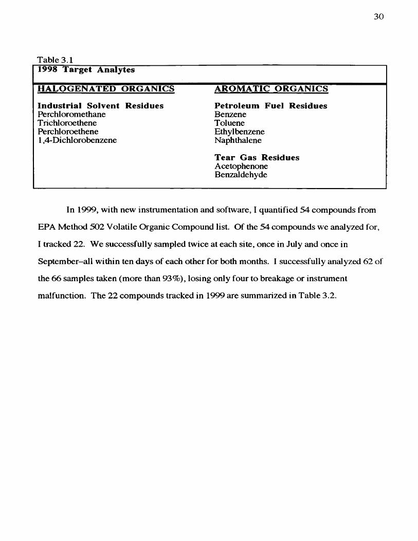
For the 1998 data, ten target analytes were chosen. Because beehive atmospheres
are extremely complex chemically, these ten compounds were chosen as they represent
several classes of compounds that have anthropogenic origins. These ten compounds also
represent chemical agents of interest found in high levels at various locations at APG. The
ten compounds are summarized in Table 3.1. The halogenated organics represent a suite of
mainly chlorinated solvents used in industrial applications. The aromatic organics are
broken into two subcategories: Petroleum Fuel Residues, representing a suite of
compounds whose source is diesel and gasoline internal combustion engines, and Tear Gas
Residues compounds that are associated with the military production and broadcast of tear
gas (Bromenshenk et al. 1997,1998,1999).
29
30
Table 3.11998 Target Analytes
HALOGENATED ORGANICS AROMATIC ORGANICS
Industrial Solvent Residues Petroleum Fuel ResiduesPerchloromethane BenzeneT richloroethene ToluenePerchloroethene Ethylbenzene1,4-Dichlorobenzene Naphthalene
Tear Gas ResiduesAcetophenoneBenzaldehyde
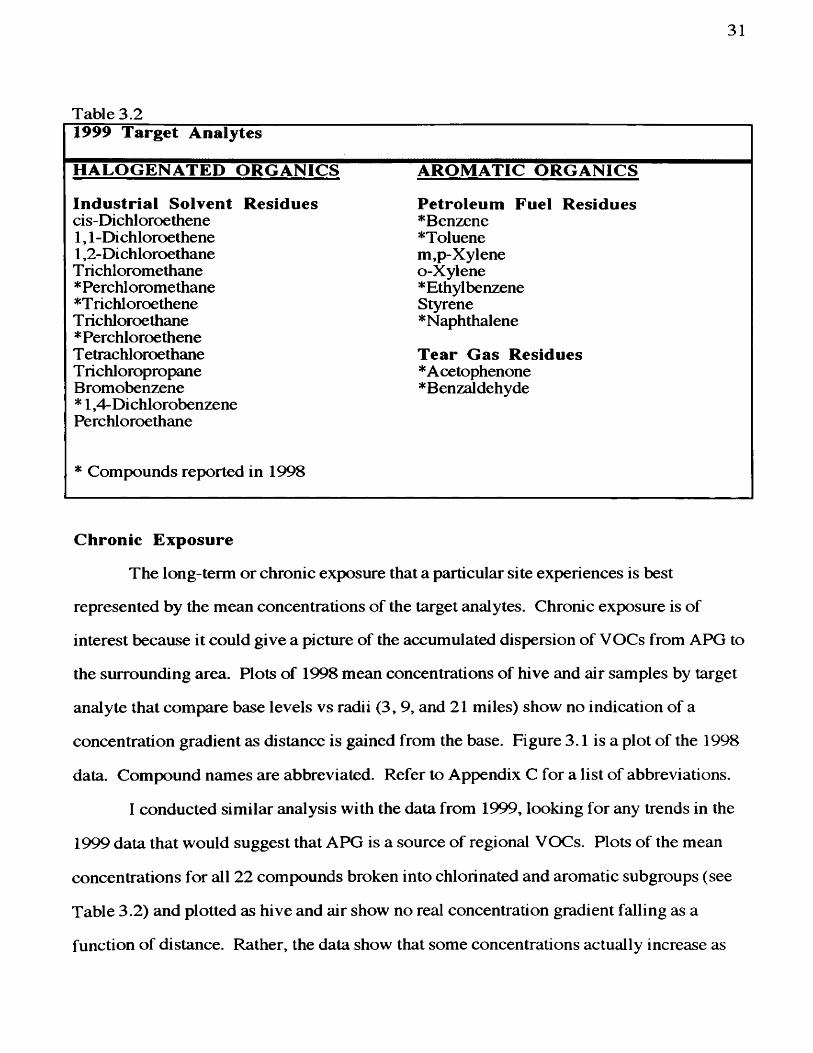
In 1999, with new instrumentation and software, I quantified 54 compounds from
EPA Method 502 Volatile Organic Compound list. Of the 54 compounds we analyzed for,
I tracked 22. We successfully sampled twice at each site, once in July and once in
September—all within ten days of each other for both months. I successfully analyzed 62 of
the 66 samples taken (more than 93%), losing only four to breakage or instrument
malfunction. The 22 compounds tracked in 1999 are summarized in Table 3.2.
31
Table 3.21999 Target Analytes
HALOGENATED ORGANICS AROMATIC ORGANICS
Industrial Solvent Residues Petroleum Fuel Residuescis-Dichloroethene *Benzene1,1-Dichloroethene ^Toluene1,2-Dichloroethane m,p-XyleneT richloromethane o-Xylene* Perchloromethane ^Ethylbenzene*T richloroethene StyreneT richloroethane ^Naphthalene* PerchloroetheneT etrachloroethane Tear Gas ResiduesT richloropropane ^AcetophenoneBromobenzene ^Benzaldehyde* 1,4-DichlorobenzenePerchloroethane
* Compounds reported in 1998
Chronic Exposure
The long-term or chronic exposure that a particular site experiences is best
represented by the mean concentrations of the target analytes. Chronic exposure is of
interest because it could give a picture of the accumulated dispersion of VOCs from APG to
the surrounding area. Plots of 1998 mean concentrations of hive and air samples by target
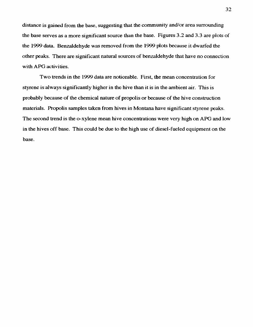
analyte that compare base levels vs radii (3, 9, and 21 miles) show no indication of a
concentration gradient as distance is gained from the base. Figure 3.1 is a plot of the 1998
data. Compound names are abbreviated. Refer to Appendix C for a list of abbreviations.
I conducted similar analysis with the data from 1999, looking for any trends in the
1999 data that would suggest that APG is a source of regional VOCs. Plots of the mean
concentrations for all 22 compounds broken into chlorinated and aromatic subgroups (see
Table 3.2) and plotted as hive and air show no real concentration gradient falling as a
function of distance. Rather, the data show that some concentrations actually increase as
32
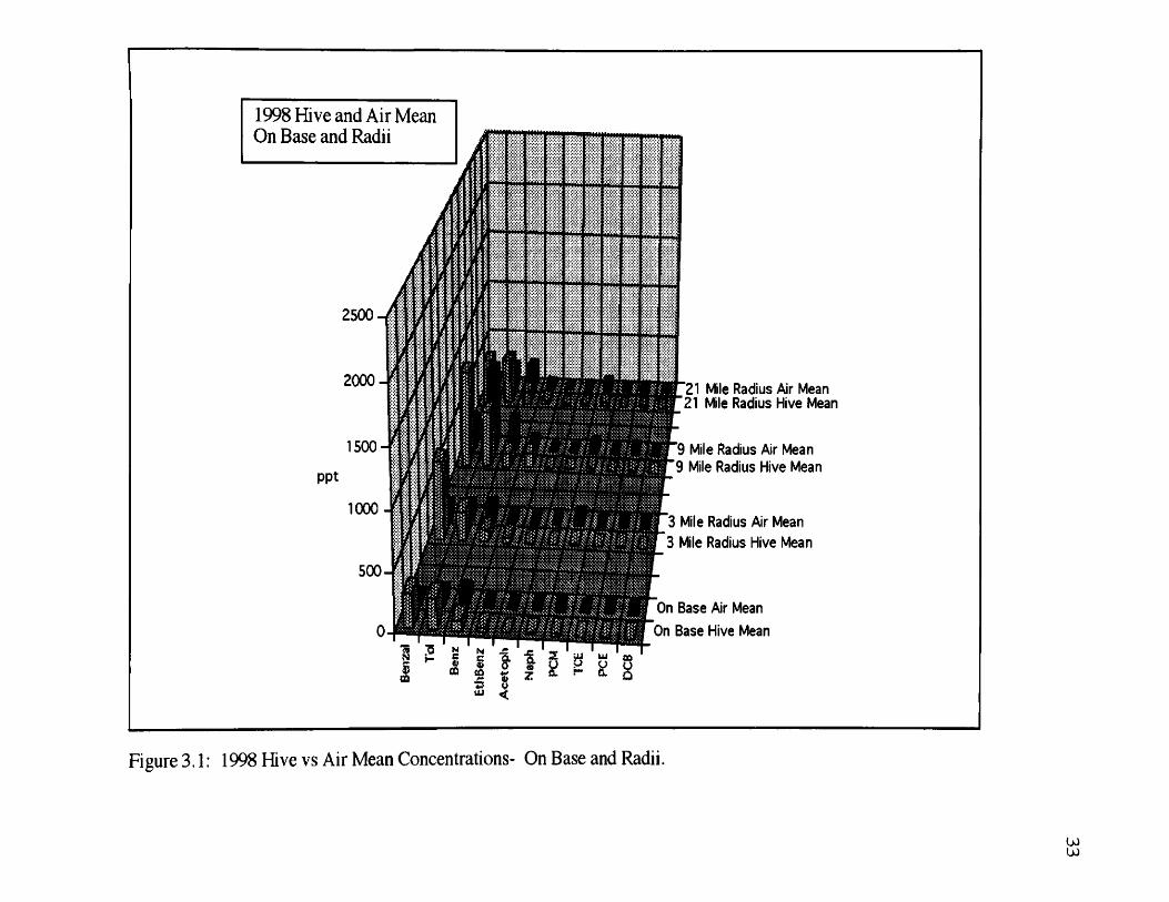
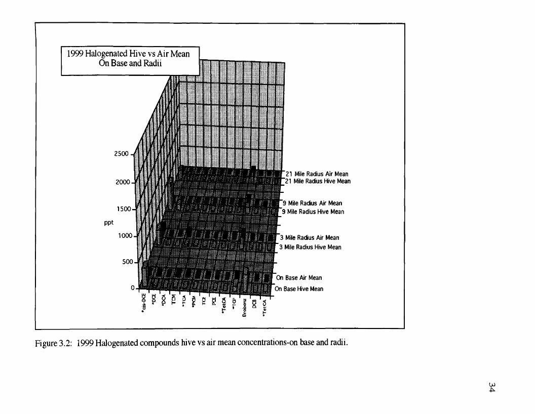
distance is gained from the base, suggesting that the community and/or area surrounding
the base serves as a more significant source than the base. Figures 3.2 and 3.3 are plots of
the 1999 data. Benzaldehyde was removed from the 1999 plots because it dwarfed the
other peaks. There are significant natural sources of benzaldehyde that have no connection
with APG activities.
Two trends in the 1999 data are noticeable. First, the mean concentration for
styrene is always significantly higher in the hive than it is in the ambient air. This is
probably because of the chemical nature of propolis or because of the hive construction
materials. Propolis samples taken from hives in Montana have significant styrene peaks.
The second trend is the o-xylene mean hive concentrations were very high on APG and low
in the hives off base. This could be due to the high use of diesel-fueled equipment on the
base.
1998 Hive and Air Mean On Base and Radii
I I 1 1 1 H ^
2000-
1 5 0 0 -
1000 -
21 Mile Radius Air Mean 21 Mile Radius Hive Mean
9 Mile Radius Air Mean 9 Mile Radius Hive Mean
3 Mile Radius Air Mean
3 Mile Radius Hive Mean
On Base Air Mean
On Base Hive Mean
Figure 3.1: 1998 Hive vs Air Mean Concentrations- On Base and Radii.
wUJ
1999 Halogenated Hive vs Air Mean On Base and Radii
2 5 0 0 - /;
2000
1 5 0 0 -^
ppt
1000
500
g § 5
21 Mile Radius Air Mean 21 Mile Radius Hive Mean
9 Mile Radius Air Mean 9 Mile Radius Hive Mean
3 Mile Radius Air Mean
3 Mile Radius Hive Mean
On Base Air Mean
On Base Hive Mean
Figure 3.2: 1999 Halogenated compounds hive vs air mean concentrations-on base and radii.
w
1999 Aromatics Hive vs Air Mean On Base and Radii
2500
2000
1500
ppt
1000
500
ta m-C
‘21 Mile Radius Air Mean "21 Mile Radius Hive Mean
9 Mile Radius Air Mean 9 Mile Radius Hive Mean
3 Mile Radius Air Mean
Mile Radius Hive Mean
On Base Air Mean
On Base Hive Mean
Figure 3.3: 1999 Aromatic compounds hive vs air mean concentrations-on base and radii.
UJun
36
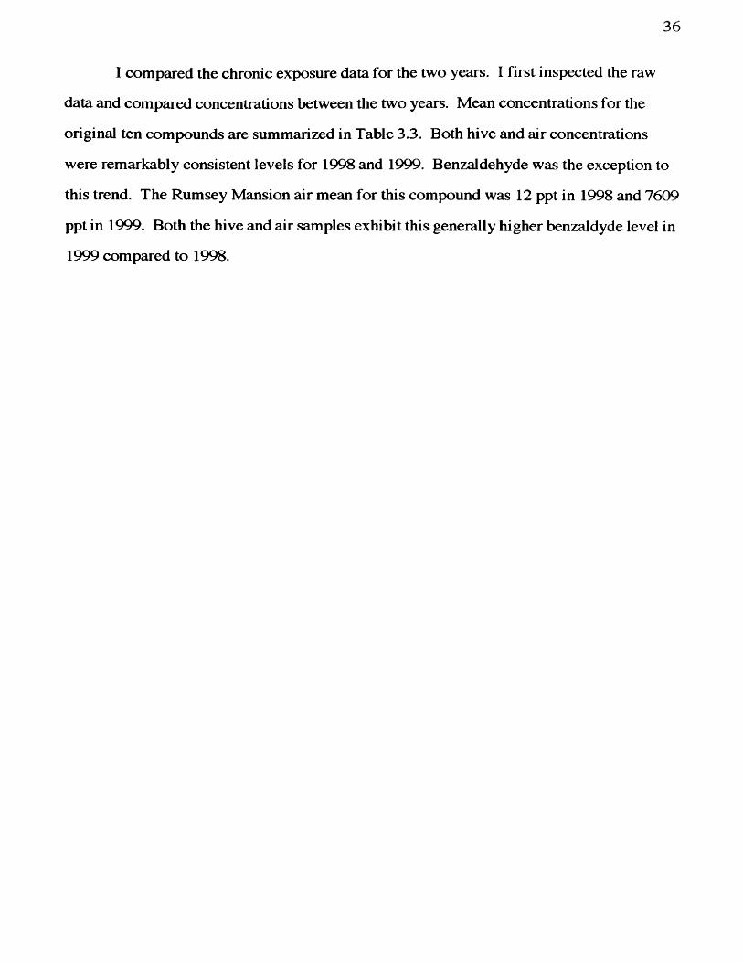
I compared the chronic exposure data for the two years. I first inspected the raw
data and compared concentrations between the two years. Mean concentrations for the
original ten compounds are summarized in Table 3.3. Both hive and air concentrations
were remarkably consistent levels for 1998 and 1999. Benzaldehyde was the exception to
this trend. The Rumsey Mansion air mean for this compound was 12 ppt in 1998 and 7609
ppt in 1999. Both the hive and air samples exhibit this generally higher benzaldyde level in
1999 compared to 1998.
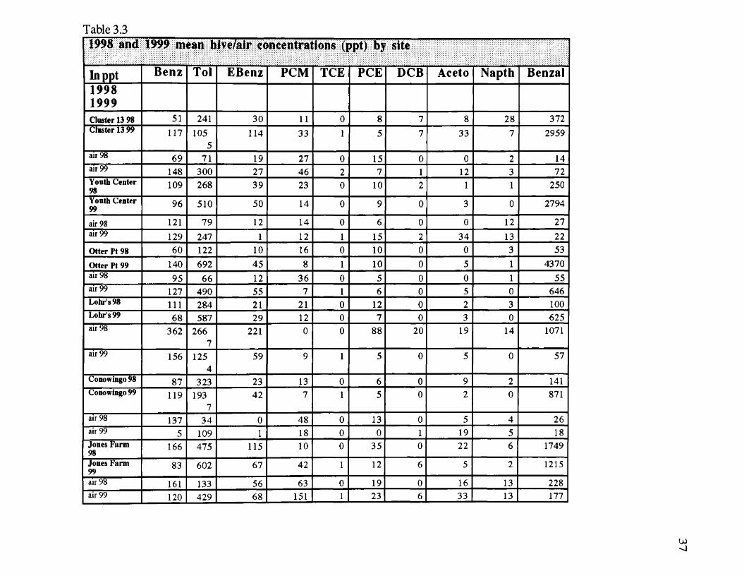
Table 3.3[ I99S m â 1999 m ew bive/nir eoneentratjons (ppt) by site
In ppt Benz Toi EBenz PCM ICE PCE DCB Aceto Napth Benzal19981999Cluster 13 98 51 241 30 11 0 8 7 8 28 372Cluster 13 99 117 105
5114 33 1 5 7 33 7 2959
air 98 69 71 19 27 0 15 0 0 2 14air 99 148 300 27 46 2 7 1 12 3 72Youth Center 98 109 268 39 23 0 10 2 1 1 250
Youth Center 99 96 510 50 14 0 9 0 3 0 2794
air 98 121 79 12 14 0 6 0 0 12 27air 99 129 247 1 12 1 15 2 34 13 22Otter Pt 98 60 122 10 16 0 10 0 0 3 53
Otter Pt 99 140 692 45 8 1 10 0 5 1 4370air 98 95 66 12 36 0 5 0 0 1 55air 99 127 490 55 7 1 6 0 5 0 646Lohr's 98 111 284 21 21 0 12 0 2 3 100Lohr's 99 68 587 29 12 0 7 0 3 0 625air 98 362 266
7221 0 0 88 20 19 14 1071
air 99 156 1254
59 9 1 5 0 5 0 57
Conowiugo 98 87 323 23 13 0 6 0 9 2 141Conowingo99 119 193
742 7 1 5 0 2 0 871
air 98 137 34 0 48 0 13 0 5 4 26air 99 5 109 1 18 0 0 1 19 5 18Jones Farm 98 166 475 115 10 0 35 0 22 6 1749
Jones Farm 99 83 602 67 42 1 12 6 5 2 1215
air 98 161 133 56 63 0 19 0 16 13 228air 99 120 429 68 151 1 23 6 33 13 177
w
Tower Hill 98 182 830 327 0 0 26 5 10 7 1321Tower Hill 99 210 107
2109 38 2 24 2 62 1 2943
air 98 159 202 20 49 0 26 0 0 5 45air 99 247 457 79 21 1 12 0 7 0 541Fairview 98 139 402 80 67 0 25 0 7 6 422Fairvicw 99 339 113
799 14 1 37 1 8 1 999
air 98 345 321 38 110 0 50 0 0 8 74air 99 387 618 77 7 0 3 0 6 0 314Ramsey 98 74 165 18 32 0 9 0 2 7 182Ramsey 99 158 732 65 28 1 7 2 39 8 1348air 98 101 108 20 52 0 7 0 0 10 12air 99 185 924 106 73 1 12 2 6 1 7609Silver Lake 98 111 394 46 40 0 10 0 2 3 1032Silver Lake 99 75 144
074 14 0 3 0 3 0 231
air 98 90 32 11 65 0 0 0 0 7 70air 99 213 297 22 5 1 1 0 1 0 212Arboretam98 160 559 30 35 0 21 0 2 1 684
Arboretam99 129 307 24 29 1 25 0 8 0 949
air 98 133 141 39 51 0 27 0 2 2 37air 99 112 256 31 14 0 24 0 2 0 245
UJ00
39
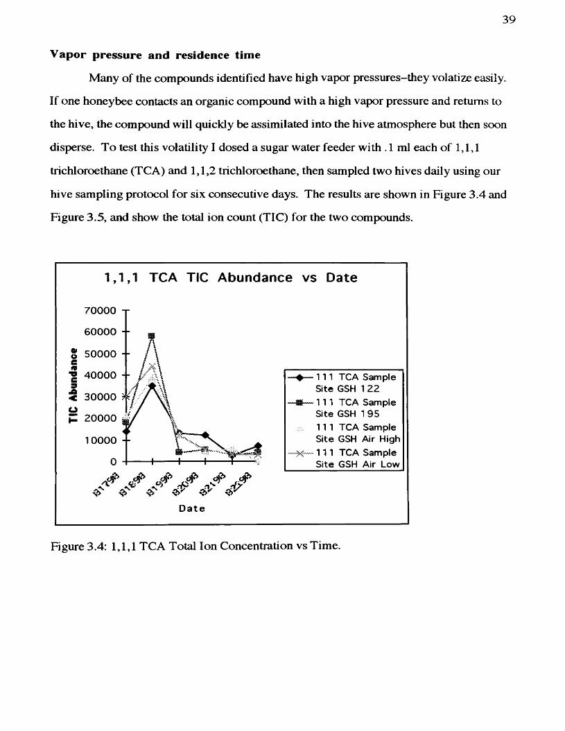
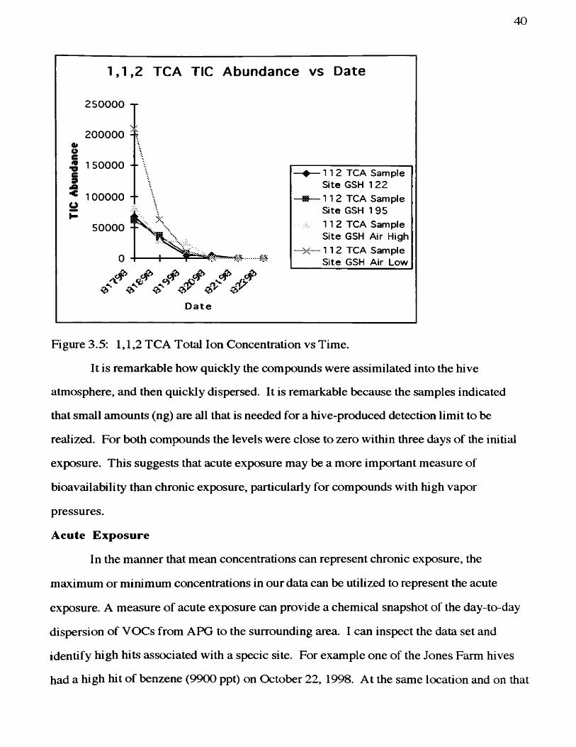
Vapor pressure and residence time
Many of the compounds identified have high vapor pressures-they volatize easily.
If one honeybee contacts an organic compound with a high vapor pressure and returns to
the hive, the compound will quickly be assimilated into the hive atmosphere but then soon
disperse. To test this volatility I dosed a sugar water feeder with .1 ml each of 1,1,1
trichloroethane (TCA) and 1,1,2 trichloroethane, then sampled two hives daily using our
hive sampling protocol for six consecutive days. The results are shown in Figure 3.4 and
Figure 3.5, and show the total ion count (TIC) for the two compounds.
1 , 1 , 1 TCA TIC Abundance vs Date
70000 T
600 0 0 --
2 50000 --
4 0 0 0 0 --
300 0 0 ^
2 0000
10000 - -
D ate
TCA SampleSite GSH 122
—# — 111 TCA SampleSite GSH 19511 1 TCA SampleSite GSH Air High
—X— 1 1 1 TCA SampleSite GSH Air Low
Figure 3.4: 1,1,1 TCA Total Ion Concentration vs Time.
40
1,1,2 TCA TIC Abundance vs Date
2 5 0 0 0 0 j
200000 4 i \S 150000 -- \
100000 - - \
50000
fe?
D a t e
—#— 112 TCA SampleSite GSH 122
— 112 TCA SampleSite GSH 195
: 1 1 2 TCA SampleSite GSH Air High112 TCA SampleSite GSH Air Low
Figure 3.5: 1,1,2 TCA Total Ion Concentration vs Time.
It is remarkable how quickly the compounds were assimilated into the hive
atmosphere, and then quickly dispersed. It is remarkable because the samples indicated
that small amounts (ng) are all that is needed for a hive-produced detection limit to be
realized. For both compounds the levels were close to zero within three days of the initial
exposure. This suggests that acute exposure may be a more important measure of
bioavailability than chronic exposure, particularly for compounds with high vapor
pressures.
Acute Exposure
In the manner that mean concentrations can represent chronic exposure, the
maximum or minimum concentrations in our data can be utilized to represent the acute
exposure. A measure of acute exposure can provide a chemical snapshot of the day-to-day
dispersion of VOCs from APG to the surrounding area. I can inspect the data set and
identify high hits associated with a specie site. For example one of the Jones Farm hives
had a high hit of benzene (9900 ppt) on October 22, 1998. At the same location and on that
41
same date, the ambient air had high benzene levels (9730 ppt). A possible explanation for
these concurrent hits might be that a small spill of fuel in the area left a liquid-phase pool
which was contacted by the bees and simultaneously evaporated into the surrounding air.
This explanation is entirely feasible because the Jones Farm is a truck farm/sales stand at
the intersection of two high volume highways. The benzene probably has no relationship to
APG as an origin.
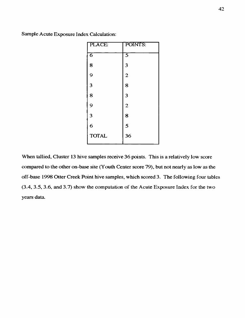
Given the large number of samples collected, the diverse sample locations, and the
assorted compounds being tracked, it was inevitable that multiple concentration spikes
would be captured. I devised a new more useful data reduction technique to estimate acute
exposure that compresses the top ten high hits for each compound for a particular site into a
single number. Termed the Acute Exposure Index its computation is as follows: First, the
hive samples were separated from the air samples. Next, the top ten hits by compound
were identified and scored. The scoring system (similar to that used in a track and field
meet) was as follows: first place receives 10 points, second place receives 9 points, third
place recieves 8 points and so on. In the case of a tie, the two sites receive equal scores
and the next place is skipped. For instance, if two sites tie for third, then both receive 8
points, then fourth place is skipped, and the next high is fifth place receiving 6 points.
Finally each site receives a total score that is a sum of its individual scores; the highest
score represents a site with relatively high acute exposure. For example, in the 1998 hive
data, samples from Cluster 13 exhibited 8 “top ten” hits (6*** in PCM, 8*** in Toi., 9* in
PCE, 3"* in DCB, 8* in Acetoph., 9** Acetoph., 3** in Naph., and ô**" in Naph).
42
Sample Acute Exposure Index Calculation:
PLACE: POINTS:
6 5
8 3
9 2
3 8
8 3
9 2
3 8
6 5
TOTAL 36
When tallied. Cluster 13 hive samples receive 36 points. This is a relatively low score
compared to the other on-base site (Youth Center score 79), but not nearly as low as the
off-base 1998 Otter Creek Point hive samples, which scored 3. The following four tables
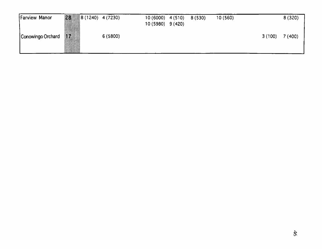
(3.4, 3.5, 3.6, and 3.7) show the computation of the Acute Exp>osure Index for the two
years data.
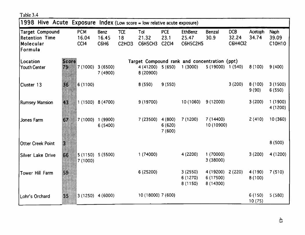
Table 3.4 _________
1998 HiVÔ Acute Exposure Index (Low score = low relative acute exposure)
Target Compound Retention Time Molecular Formula
Location Youth Center
Cluster 13
PCM16.04CCI4
Benz16.45C6H6
TCE Toi PCE 18 21.32 23.1C2HCI3 C6H5CH3 C2CI4
EthBenz Benzal25.47 30.9C6H5C2H5
DCB Acetoph Naph32.24 34.74 39.09C6H4CI2 C10H10
'Siftoh7 8 - ; . 7(1000) 3 (6500) , ' 7(4900)
M , 6 ( 1100)
Rumsey Mansion 4 3 • 1 (1500) 8(4700)
Jones Farm 7(1000) 1 (9900) ; " 6(5400)
Otter Creek Point 3 ' -
Silver Lake Drive 5(1150) 5 (5500) 7(1000)
Tower Hill Farm :s9
Lohr's Orchard 35 3(1250) 4(6000)
Target Compound rank and concentration (ppt)4(41200) 5(650) 1 (3000) 5(19000) 1 (540) 8(100) 9(400)8 (20900)
8 (550) 9(550)
9(19700) 10(1060) 9(12000)
7(23500) 4(800) 7(1200) 7(14400)6(620) 10(10900)7(600)
1 (74000)
6 (25200)
4(2200) 1 (70000)3(38000)
3(200) 8(100) 3(1500)9(90) 6(550)
3(200) 1 (1900)4(1200)
2(410) 10(360)
8(500)
3(200) 4(1200)
10(18000) 7(600)
3(2550) 4(19200) 2(220) 4(190) 7(510)6(1270) 6(17500) 8(100)8(1150) 8(14300)
6(150) 5(580)10 (75)
6
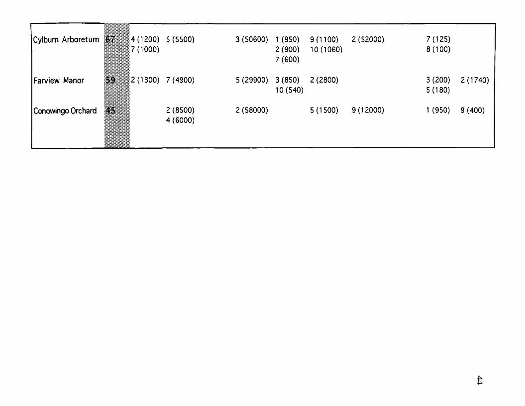
Cylburn Arboretum ?67 *4 (1200) 5 (5500) * -7 (1000)
3 (50600) 1 (950) 9 (1100) 2 (52000)2 (900) 10 (1060)7(600)
7(125)8 ( 100)
Farview Manor 2 (1300) 7 (4900) 5 (29900) 3 (850) 2 (2800)10(540)
3 (200) 2(1740)5(180)
Conowingo Orchard . : 2(8500) 4(6000)
2(58000) 5(1500) 9(12000) 1 (950) 9(400)
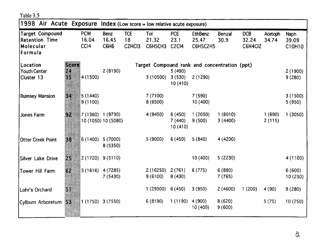
Table 3.5____________________________________________________________________
1998 Air Acute Exposure index (Low score low relative acute exposure)
Target Compound Retention Time M olecular Formula
PCM16.04CCI4
Benz16.45C6H6
TCE Toi 18 21.32 C2HCI3 C6H5CH3
PCE23.1C2CI4
EthBenz25.47C6H5C2H5
Benzal30.9
DCB Acetoph 32.24 34.74 C6H4CI2
Naph39.09C10H10
Location Youth Center Cluster 13
S c o rf 24 '35 -4(1500)
2(8190)Target Compound rank
5(490)3 (10500) 3 (530)
10(410)
and concentration (ppt)
2 (1290)2(1900) 9(280)
Rumsey Mansion 34 5 (1440) 9(1100)
7(7100) 8(6500)
7(590) 10(400)
3 (1500) 5(950)
Jones Farm , '7 (1360) 10(1050)
1 (9730) 10 (5080)
4(9450) 6(450)7(440) 10(410)
1(2050) 9(500)
1 (6010) 3(4400)
1 (690) 2(115)
1 (3050)
Otter Creek Point 3% '6(1400) 5(7000) 8 (5350)
5(9000) 6(450) 5(840) 4(4200)
Silver Lake Drive 25 2(1720) 9(5110) 10 (400) 5(2230) 4(1100)
Tower Hill Farm m 3(1616) 4(7285) 7(5430)
2 (16250) 9(6100)
2(761) 8(430)
6 (775) 6(880) 7 (765)
6(600) 10(250)
Lohr's Orchard 51 1 (29300) 6(450) 3(950) 2(4600) 1 (200) 4(90) 9(280)
Cylburn Arboretum 53 1 (1750) 3 (7550) 6(8190) 1 (1190) 4(900) 10(400)
8(620) 9(600)
5(75) 10 (250)
Farview Manor 2$. 8(1240) 4(7230) 10(6000) 4(510) 8(530)10 (5980) 9 (420)
10 (560)
Conowingo Orchard î 7 6(5800)
8 (320)
3(100) 7(400)
&
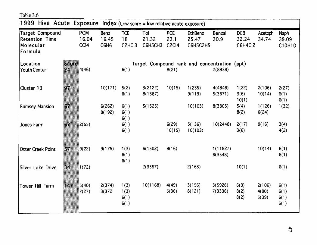
Table 3.6
1999 Hivô Acute Exposure Index (Low score = low relative acute exposure)
Target Compound PCM Benz TCE Toi PCE EthBenz Benzal DCB Acetoph NaphRetention Time 16.04 16.45 18 21.32 23.1 25.47 30.9 32.24 34.74 39.09Molecular CCI4 C6H6 C2HCI3 C6H5CH3 C2CI4 C6H5C2H5 C6H4CI2 C10H10Formula
Location Target Compound rank and concentration (ppt)Youth Center ^ 4 . 4(46) 6(1) 8(21) 2(8938)
Cluster 13 i r [ . 10(171) 5(2) 3(2122) 10(15) 1(235) 4(4846) 1(22) 2(106) 2(27)6(1) 8(1387) 9(119) 5(3671) 3(6) 10(14) 6(1)
10(1) 6(1)Rumsey Mansion 6(262) 6(1) 5(1 525) 10(103) 8(3305) 5(4) 1(126) 1(32)
8(192) 6(1) 8(2) 6(24)6(1)
Jones Farm 67 ; 2(55) 6(1) 6(29) 5(136) 10(2448) 2(17) 9(16) 3(4)6(1) 10(15) 10(103) 3(6) 4(2)
Otter Creek Point 57 9(22) 9(175) 1(3) 6(1502) 9(16) 1(11827) 10(14) 6(1)6(1) 6(3548) 6(1)6(1)
Silver Lake Drive 34 ' 1(72) 2(3557) 2(163) 10(1) 6(1)
Tower Hill Farm Î47 5(40) 2(374) 1(3) 10(1168) 4(49) 3(156) 3(5926) 6(3) 2(106) 6(1)' 7(27) 3(372 1(3) 5(36) 8(121) 7(3336) 8(2) 4(90) 6(1)
6(1) 8(2) 5(39) 6(1)6(1) 6(1)
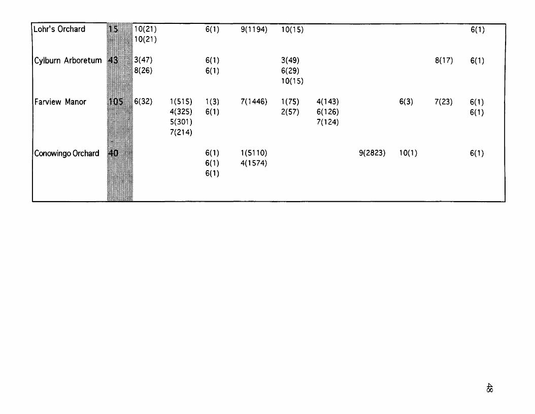
Lohr’s Orchard 15 10(21) \ 10(21)
6(1) 9(1194) 10(15) 6(1)
Cylburn Arboretum 4 3 ' ' 3(47) ' ; 8(26)
6(1)6(1)
3(49)6(29)10(15)
8(17) 6(1)
Farview Manor . m ' 6(32)
S I M
1(515)4(325)5(301)7(214)
1(3)6(1)
7(1446) 1(75)2(57)
4(143)6(126)7(124)
6(3) 7(23) 6(1)6(1)
Conowingo Orchard 6(1)6(1)6(1)
1(5110)4(1574)
9(2823) 10(1) 6(1)
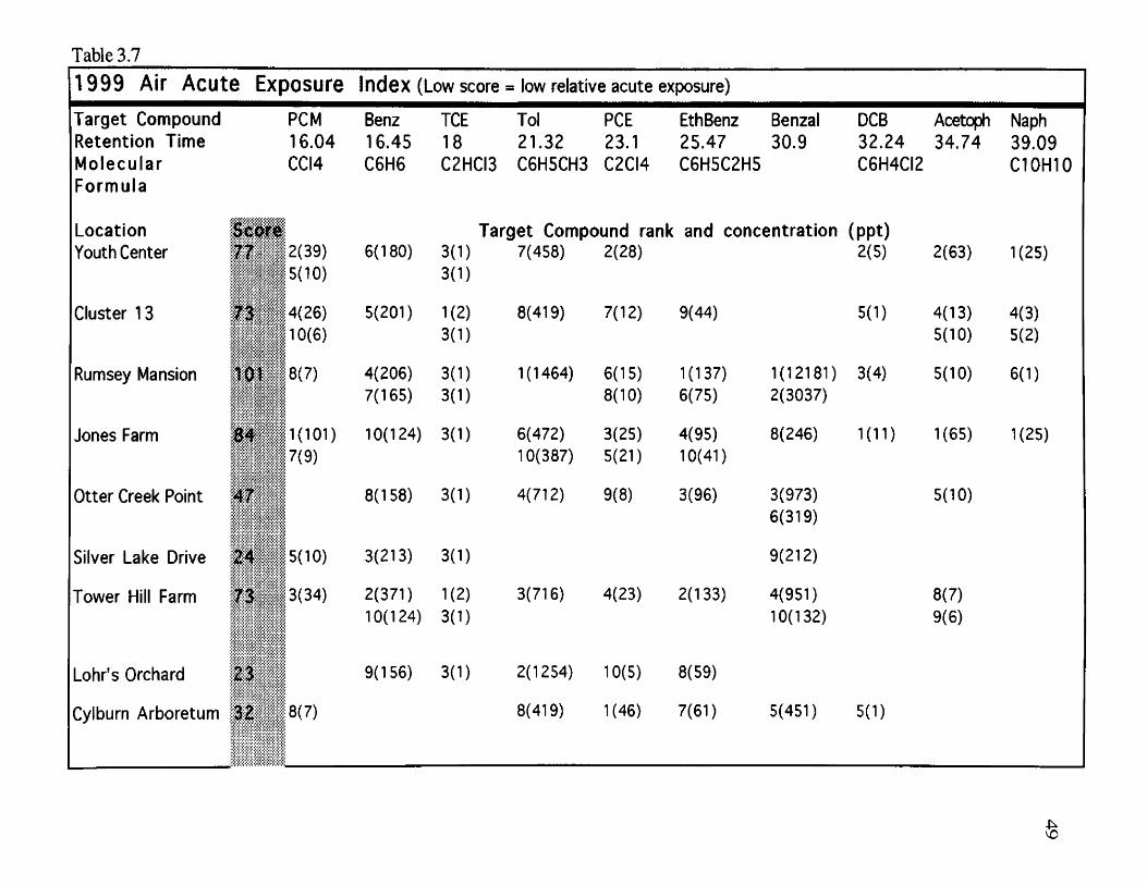
Table 3.7
1999 Air Acute Exposure Index (Low score » low relative acute exposure)
Target Compound Retention Time Molecular Formula
PCM16.04CCI4
Benz16.45C6H6
TCE Toi 18 21.32 C2HCI3 C6H5CH3
PCE23.1C2CI4
EthBenz25.47C6H5C2H5
Benzal30.9
DCB32.24C6H4CI2
Acetoph34.74
Naph39.09C10H10
Location Youth Center
Score77- 2(39)
5(10)6(180) 3(1)
3(1)
Target Compound rank and concentration (ppt)7(458) 2(28) 2(5) 2(63) 1(25)
Cluster 13 7 3 / 4(26)10(6)
5(201) 1(2)3(1)
8(419) 7(12) 9(44) 5(1) 4(13)5(10)
4(3)5(2)
Rumsey Mansion 101 8(7) 4(206)7(165)
3(1)3(1)
1(1464) 6(15)8(10)
1(137)6(75)
1(12181)2(3037)
3(4) 5(10) 6(1)
Jones Farm 84 ' 1(101)7(9)
10(124) 3(1) 6(472)10(387)
3(25)5(21)
4(95)10(41)
8(246) 1(11) 1(65) 1(25)
Otter Creek Point 47 " 8(158) 3(1) 4(712) 9(8) 3(96) 3(973)6(319)
5(10)
Silver Lake Drive 24, 5(10) 3(213) 3(1) 9(212)
Tower Hill Farm 73 3(34) 2(371)10(124)
1(2)3(1)
3(716) 4(23) 2(133) 4(951)10(132)
8(7)9(6)
Lohr's Orchard 23 9(156) 3(1) 2(1254) 10(5) 8(59)
Cylburn Arboretum 32 8(7) 8(419) 1(46) 7(61) 5(451) 5(1)
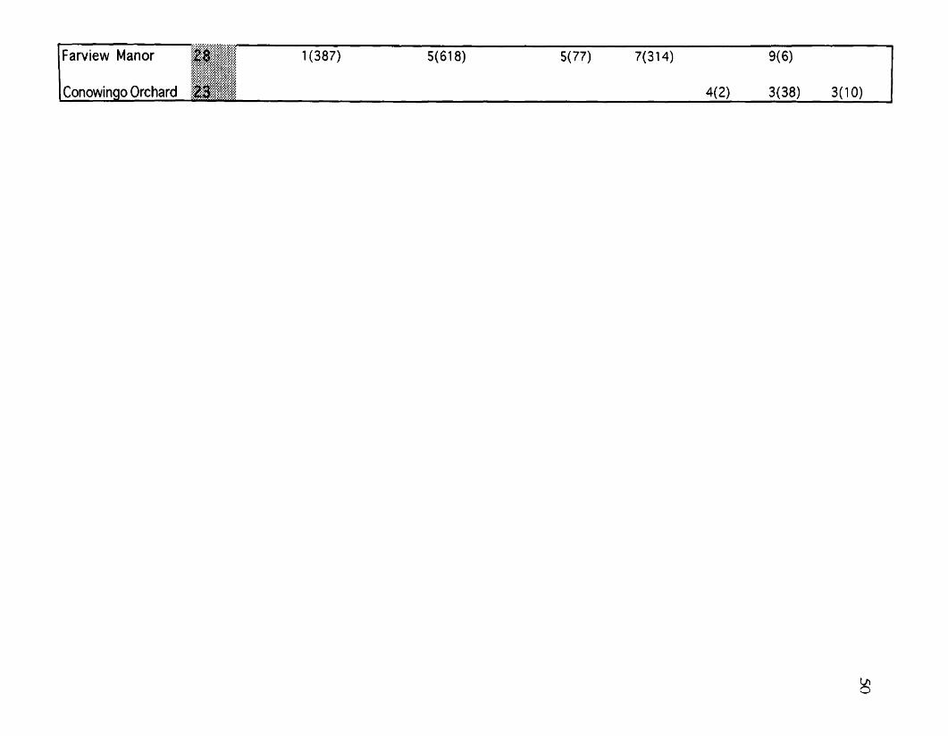
Farview Manor m m s 1(387) 5(618) 5(77) 7(314) 9(6)
Conowingo Orchard 4(2) 3(38) 3(10)
o&
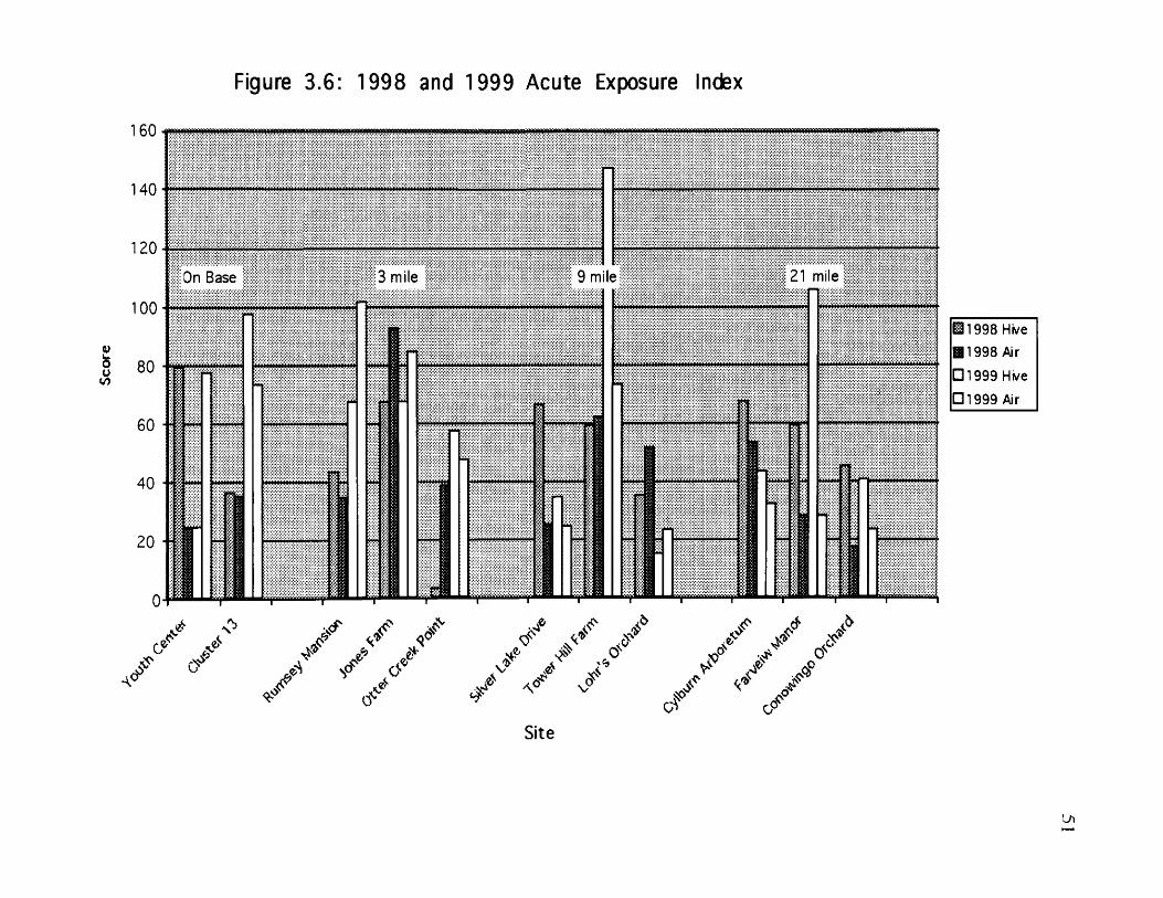
Figure 3.6: 1998 and 1999 Acute Exposure Index
21 mile3 mile 9 mileOn Base
OTiximi>if>iiiïyiï1|l ï l l i V r m l l ï i ^ Y .
^ 1 9 9 8 H we
a 1998 Air
□ 1999 Hive
□ 1999 Air
O&
é¥
/ y V**oîr
/ / /Site
LA
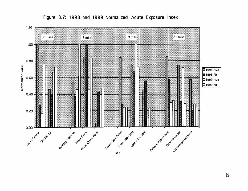
Figure 3.7: 1998 and 1999 Normalized Acute Exposure Index
1.20
"OVN
1z
21 mileOn Base 9 mile
1 1 9 9 8 HK/e
a 1998 Air
□ 1999 Hive
□ 1999 Air
S ite
«
53
Several trends emerge from the Acute Exposure Index system. First, Jones Farm
and Tower HiII Farm score high in both the hive and air. These areas share a similar
intensity of activity, namely automobile and truck traffic and use of agrochemicals. They
differ in their proximity to APG. Jones Farm is 3 miles from APG and Tower Hill Farm is
9 miles away.
The second trend is that the generally low scoring sites - Otter Creek Point, Silver
Lake Drive, Lohr’s Orchard, and Conwingo Orchard — have relatively low activity and are
fairly well isolated and heavily vegetated. These four sites vary in distance from 3 to 21
miles from APG.
Motor vehicles are the dominant contributor to VOC emissions and the major
sources of alkane and aromatic emissions in the United States (Seinfeld 1998). These
evaporative emissions fall into four categories: hot-soak emmissions - vaporization of fuel
from heat after the engine has been shut off ; running losses - vaporization of fuel while the
engine is operating; resting losses — fuel leaks and diffusion through contaminated
containment materials; and refueling losses — fuel vapor displacement during filling of the
fuel tank (Seinfeld 1998). It follows then that areas with low automobile exposure would
score low and areas with high automobile exposure would score high.
Another trend is the apparently high scores for the 1999 hive data at Cluster 13
(97), Towerhill Farm (147), and Farview Manor (105). These scores are probably inflated
values because of the repeated high scoring of relatively low hits of TCE (all 3 ppt or less)
at the two sites. When the scoring values are normalized TCE hits still contribute to the
score but are not prominent, and the trend fades. The fact that I had several TCE hits in
1999 and very few in 1998 is probably a function of the new instrumentation.
The sensitivity of the data reduction technique enabled me to recognize the effects of
a known activity. Cluster 13 showed remarkably higher scores for the hive and air in 1999
versus 1998. I traced these increases high hits for benzene and ethylbenzene in 1999 that
were not present in 1998. Benzene and ethylbenzene are part of the BTEX class of
54
compounds normally associated as fossil fuel residues. At Cluster 13, a removal action in
1999 generated substantial local truck activity. This removal action did not occur in 1998.
The Acute Exposure Index system I devised does not show any trend that suggests
APG is a regional source of bioavailable VOCs. In order to confirm the lack of significant
directional trends and to ascertain contributing sources of variation I performed an analysis
of variance (ANOVA) on the data.
Analysis o f Variance
Because the data set for 1999 is fairly complete a multivariate analysis of variance
was conducted using the General Linear Model (GLM) procedure with SPSS v. 8.0
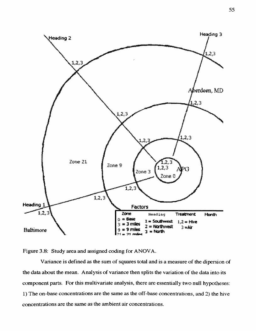
software. It is a complete random design with four independent variables (Treatment,
Zone, Heading, and Month) and all interactions included. The Treatment is defined as the
hive air versus the ambient air sampled. The Zone is the distance in miles (3, 9, 21) from
APG with 0 being the on-base sites. The 0 Zone is not completely replicated because there
are only two rather than three sites. The Heading is the three transects radiating from the
base (1, 2, 3). The Month represents the pooled July and September dates assuming the
season and not the day was the focus of the sampling. Each factor was assumed to be
fixed, that is, it is intended to represent only the intervals sampled and does not represent
randomly sampled intervals from a larger distribution. Figure 3.8 shows the study area and
coding assigned to the different factors.
55
lerd erL, MD
H e a d in g
Î « ScuMmtsl i;z ^ MW à-j^r
3 « MQMM
Figure 3.8: Study area and assigned coding for ANOVA.
Variance is defined as the sum of squares total and is a measure of the dipersion of
the data about the mean. Analysis of variance then splits the variation of the data into its
component parts. For this multivariate analysis, there are essentially two null hypotheses:
1) The on-base concentrations are the same as the off-base concentrations, and 2) the hive
concentrations are the same as the ambient air concentrations.
56
Prior to the analysis of variance, the dependent variables—the 22 VOC
concentrations-were subject to a principal components analysis. The purpose of this
analysis was to reduce the number of variables to a smaller subset of linear combinations.
The results of the analysis revealed eight principal components accounted for 75% of the
variation among the original dependent variables. These eight standardized principal
components were then subject to analysis of variance by the GLM procedure.
The Wilks’ Lambda Multivariate test is the first step of the analysis of variance used
to identify which of the interactions between the independent variables- Treatment, Zone,
Heading, Month-showed a significant difference in at least one of the principal
components. The significance value is the probability that there is at least one significant
difference in the principal components. A .05 critical value (95% confidence level) was
chosen because it is used in litigation and in the scientific literature for this type of
environmental research (Henderson 2001). Using this critical value, of all expected
observations, 95% are within 1.96 standard deviations of the mean. Thus any value ^.05
indicates an important interaction that random measurement error cannot explain. The
observed power is a measure of whether or not a real difference will be missed. High
values of observed power indicate a low likelihood that a real difference has been missed as
a result of the analysis.
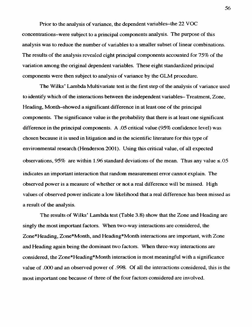
The results of Wilks’ Lambda test (Table 3.8) show that the Zone and Heading are
singly the most important factors. When two-way interactions are considered, the
Zone* Heading, Zone* Month, and Heading*Month interactions are important, with Zone
and Heading again being the dominant two factors. When three-way interactions are
considered, the Zone*Heading*Month interaction is most meaningful with a significance
value of .000 and an observed power of .998. Of all the interactions considered, this is the
most important one because of three of the four factors considered are involved.
57
Table 3 .8Wilks^ Lambda Multivariate Test ResultsInteraction Significance
(.05 critical value)Observed Power
One-wayTreatment .084 .671Zone .956Aeajmg MiMonth .140 .581T w o-w ayT reatment*Zone .641 .435T reatment* Heading .859 .308Zc»ie*Hcading mmmÊÊrnimmÊÊÊmËm .999T reatmemt*Month .199 .512Zone^Mtmth ,000 .997Heading* Month ,000 ,999Three-wayT reatment* Zone* Heading .260 .660T reatment*Zone* Month .875 .155T reatment* Heading* Month .210 .501
m m : ' - : smFour-wayT reatment*Zone* Headi ng* Month .514 .304
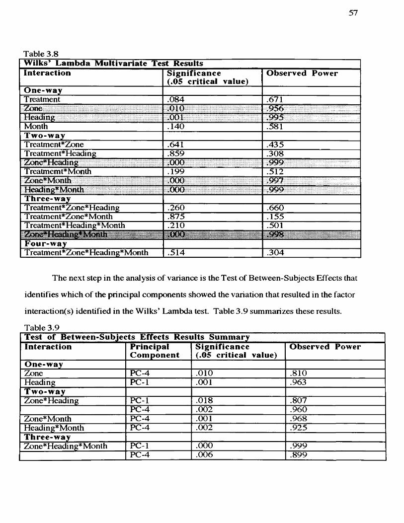
The next step in the analysis of variance is the Test of Between-Subjects Effects that
identifies which of the principal components showed the variation that resulted in the factor
interaction(s) identified in the Wilks’ Lambda test. Table 3.9 summarizes these results.
Table 3.9Test of Between-Subjects Effects Results SummaryInteraction Principal
ComponentSignificance (.05 critical value)
Observed Power
One-wayZone PC-4 .010 .810Heading PC-1 .001 .963T w o-w ayZone* Heading PC-1 .018 .807
PC-4 .002 .960Zone* Month PC-4 .001 .968Heading* Month PC-4 .002 .925Three-wayZone*Heading* Month PC-1 .000 .999
PC-4 .006 .899
58
The results of this part of the analysis show that only two of the eight principal
components (PC-1 and PC-4) play a significant role in the variation in the data set. PC-1,
which accounts for 17% of the total variation, strongly influences the three-way
Zone*Heading* Month interaction and to a lesser extent the Zone*Heading and Heading
interactions. PC-4, which accounts for 9% of the total variation, influences the
Zone*Heading*Month, Zone*Heading, Zone*Month, Heading*Month, and Zone
interactions.
PC-1 is a weighted average of gasoline components made up primarily of benzene,
ethylbenzene, and m- and p-xylene with small contributions of dichloromethane and
trichloroethene. PC-4 is a contrast between levels of benzene and perchloroethene, and
dichloromethane and toluene — as benzene and perchloroethene levels increase,
dichloromethane and toluene levels decrease and viceversa
The final step in the multivariate analysis considers plots of the estimated marginal
means of PC-1 and PC-4. Estimated marginal means are weighted averages of the
variation in the principal component and help to further identify the source of variation
within the principal component. Specific plots for PC-1 and PC-4 will be considered
individually.
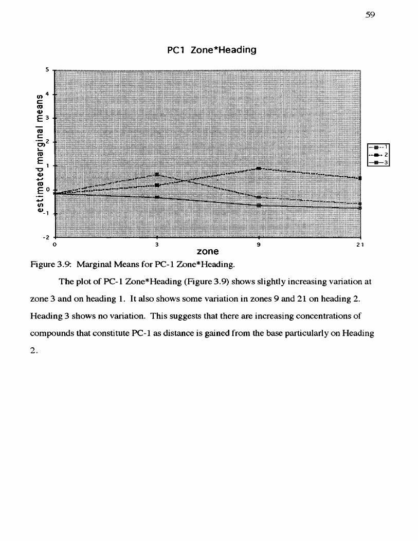
59
PCI Zone*Heading
CD
<1>
(/)<u
-2O 3 9 2 1
—% 1
—%—3
zoneFigure 3.9: Marginal Means for PC-1 Zone*Heading.
The plot of PC-1 Zone*Heading (Figure 3.9) shows slightly increasing variation at
zone 3 and on heading 1. It also shows some variation in zones 9 and 21 on heading 2.
Heading 3 shows no variation. This suggests that there are increasing concentrations of
compounds that constitute PC-1 as distance is gained from the base particularly on Heading
2 .
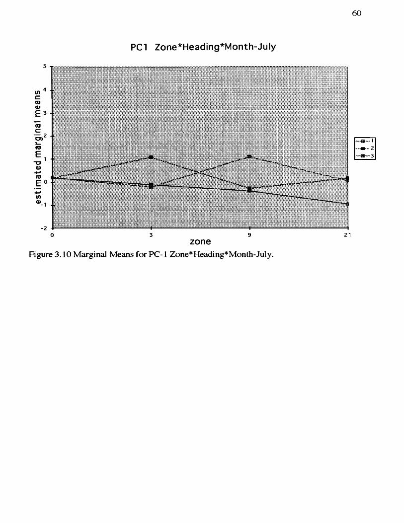
PCI Zone*Heading*Month-July
60
CD
c
3 9 2 10
— M — 3
zoneFigure 3.10 Marginal Means for PC-1 Zone*Heading*Month-July.
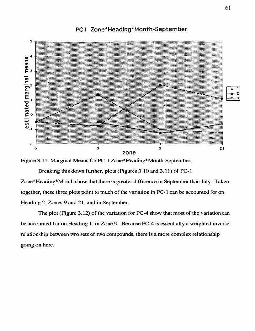
61
PCI Zone*Heading*Month-September
c<D
<L>■*-*CDE o
o>
- 20 3 9 21
—SS—3
zoneFigure 3.11: Marginal Means for PC-1 Zone*Heading*Month-September.
Breaking this down further, plots (Figures 3.10 and 3.11) of PC-1
Zone*Heading*Month show that there is greater difference in September than July. Taken
together, these three plots point to much of the variation in PC-1 can be accounted for on
Heading 2, Zones 9 and 21, and in September.
The plot (Figure 3.12) of the variation for PC-4 show that most of the variation can
be accounted for on Heading 1, in Zone 9. Because PC-4 is essentially a weighted inverse
relationship between two sets of two compounds, there is a more complex relationship
going on here.
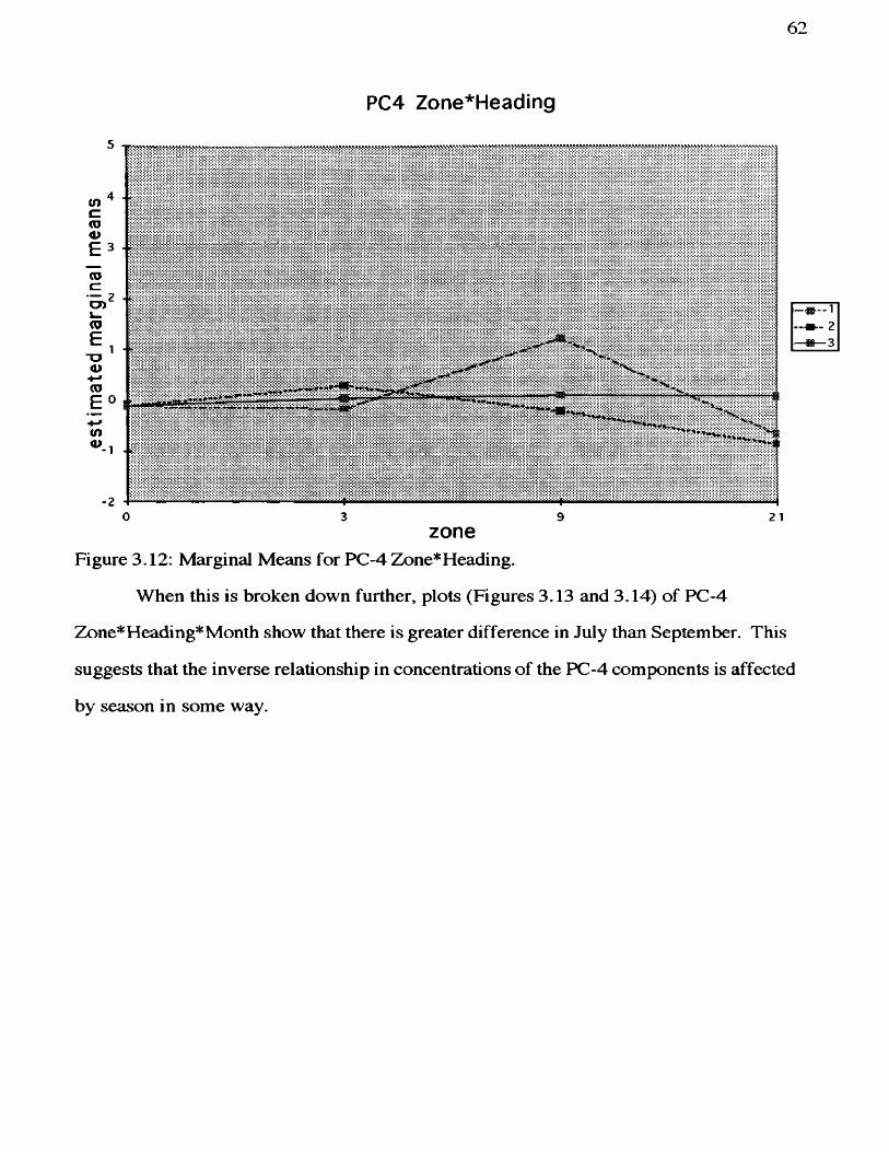
62
PC4 Zone*Heading
(0
(Oc
(D
------- -
0 3 9 21
- 1- 2
3
zoneFigure 3.12: Marginal Means for PC-4 Zone*Heading.
When this is broken down further, plots (Figures 3.13 and 3.14) of PC-4
Zone*Heading*Month show that there is greater difference in July than September. This
suggests that the inverse relationship in concentrations of the PC-4 components is affected
by season in some way.
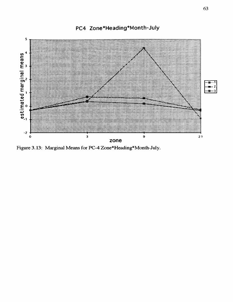
PC4 Zone*Heading*Month-July
63
inCD
<D
20 3 9 2 1
— %— 3
zoneFigure 3.13: Marginal Means for PC-4 Zone*Heading*Month-July.
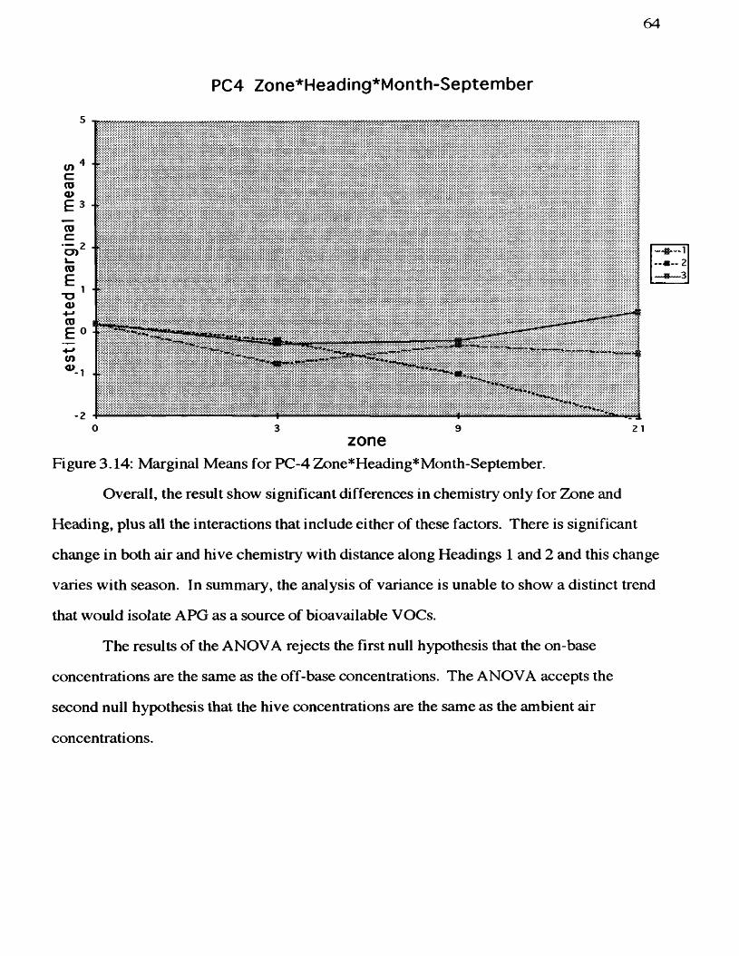
PC4 Zone*Heading*Month-September
64
tncCDo>
CDC— — 1 —- — 2
TD<U
<n<u
0 3 9 2 1zone
Figure 3.14: Marginal Means for PC-4 Zone*Heading*Month-September.
Overall, the result show significant differences in chemistry only for Zone and
Heading, plus all the interactions that include either of these factors. There is significant
change in both air and hive chemistry with distance along Headings 1 and 2 and this change
varies with season. In summary, the analysis of variance is unable to show a distinct trend
that would isolate APG as a source of bioavailable VOCs.
The results of the ANOVA rejects the first null hypothesis that the on-base
concentrations are the same as the off-base concentrations. The ANOVA accepts the
second null hypothesis that the hive concentrations are the same as the ambient air
concentrations.
CHAPTER 4: DISCUSSION AND CONCLUSIONS.
This chapter discusses the results of samples from the two field seasons, addresses
the conclusions drawn from the distribution and concentrations of VOCs around APG,
and finishes with suggestions for further study.
Discussion
This study was initiated to address the concerns of the local surrounding
community. The concerns were whether or not VOCs were drifting off the base and into
the local community causing elevated health risks. The honeybees were used in this
study to determine if the VOCs on the proving ground were bioavailable to honeybees off
the proving ground. By extension, if VOCs are bioavailable off base then they could be
available to humans occupying the area surrounding APG.
Health Risk Comparison
The most important end use of the APG boundary study is an assessment of the
human health impacts posed by the chemical concentrations measured in the study.
Comparisons of my sample concentrations for select compounds can be made to
published workplace Threshold Limit Values (TLV). Table 4.1 shows the time weighted
average (TWA) and ceiling TLVs and maximum concentrations in hive and air for the
two field seasons.
65
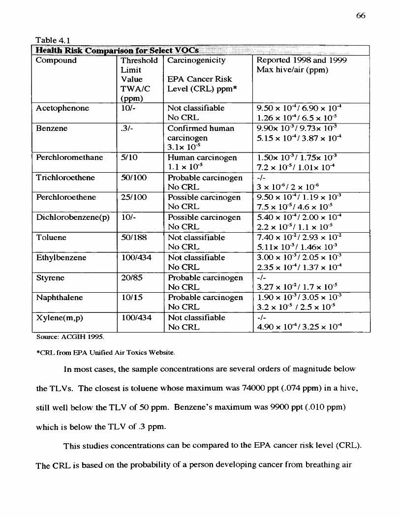
6 6
Table 4.1
Compound ThresholdLimitValueTWA/C(ppm)
Carcinogenicity
EPA Cancer Risk Level (CRL) ppm*
Reported 1998 and 1999 Max hive/air (ppm)
Acetophenone 10/- Not classifiable No CRL
9.50 X 10^/ 6.90 X 10- 1.26 X 10- / 6.5 X 10 ^
Benzene 31- Confirmed human carcinogen 3.1x 10^
9.90x 10 /9 .73X 10' 5.15 X 10*^/3.87 X 10-
Perchloromethane 5/10 Human carcinogen1.1 X 10^
1.50x 10^/ 1.75x 10^ 7.2 X 10^/ l.Olx 10^
T richloroethene 50/100 Probable carcinogen No CRL
-/-3 X lO V 2 X 10^
Perchloroethene 25/100 Possible carcinogen No CRL
9.50 X 10-^/ 1.19 X 10 7.5 X 10 ^/4.6 X 10 ^
Dichlorobenzene(p) 10/- Possible carcinogen No CRL
5.40 X 10- / 2.00 X W2.2 X 10'^/ 1.1 X 10 ^
T oluene 50/188 Not classifiable No CRL
7.40 X 10 ^/ 2.93 X 10 5.11X 10^/ 1.46X 10
Ethylbenzene 100/434 Not classifiable No CRL
3.00 X 10 / 2.05 X 10 2.35 X 10- / 1.37 X 10"*
Styrene 20/85 Probable carcinogen No CRL
-/-3.27 X 10 ^/ 1.7 X 10 ^
Naphthalene 10/15 Probable carcinogen No CRL
1.90 X 10 /3.05 X 10 3.2 X 10^ / 2.5 X 10^
Xylene(m,p) 100/434 Not classifiable No CRL
-/-4.90 X 10"*/3.25 X 10"*
Source: ACGIH 1995.
*CRL from EPA Unified Air Toxics Website.
In most cases, the sample concentrations are several orders of magnitude below
the TLVs. The closest is toluene whose maximum was 74000 ppt (.074 ppm) in a hive,
still well below the TLV of 50 ppm. Benzene’s maximum was 9900 ppt (.010 ppm)
which is below the TLV of .3 ppm.
This studies concentrations can be compared to the EPA cancer risk level (CRL).
The CRL is based on the probability of a person developing cancer from breathing air
67
containing a specified concentration of a chemical. The EPA estimates that, if an
individual were to breathe air containing benzene at 31 ppt over his or her entire lifetime,
that person would theoretically have no more than a one-in-a-million increased chance of
developing cancer as a direct result of breathing air containing this chemical. However,
the mean concentrations of benzene for the various sites exceed the EPA lifetime cancer
risk level of 3 1 ppt by a factor of between two to twelve. Fairveiw Manor had the highest
means of 387 ppt in the 99 air and 345 ppt in the 98 air. This twelve times the CRL is
probably a result of the revolatization during refueling at the adjacent gas station.
Similarly the perchloromethane mean concentrations exceed the 11 ppt /one-in-a million
CRL by a factor of two to thirteen with Jones Farm having the highest mean in the 99 air
samples (151 ppt).
In all likelihood, the VOC contamination that exists in the study area is
attributable to local sources and regional sources other than APG. Northeastern
Maryland and the Baltimore area are highly populated and heavily industrialized. The
1999 Maryland Air Quality Data Report shows EPA ozone attainment to be designated as
“non-attained” and classified as “severe” for the City of Baltimore, Baltimore County,
Harford County, and Cecil County. This is significant because ozone concentration is
directly related to VOC concentration via a series of photochemical reactions (Seinfeld
1998). At specific sites in this region, natural and anthropogenic local emissions dictate
the air quality and air chemistry. That is not to say that APG does not influence the air
quality in the region, but the APG influence is secondary or even tertiary and is more
than likely masked by local emissions. The Maryland Department of the Environment
6 8
(MDE) estimated the top ten contributors to VOC emissions in the Baltimore area (Table
4.2). None of these relate to APG-specific activities.
My results show that APG does not appear to be a source of regionally distributed
bioavailable VOCs. VOCs do not seem to be dispersed from the base as a function of
distance or direction. Are these results valid or have other factors created a more
complex picture? There are several complicating factors that contribute to the lack of an
apparent dispersal pattern of VOCs from the base. Those factors include bee exposure
routes, photochemical decay reactions, and wind direction. All could play a role in the
disruption of a dispersal pattern.
Bee Exposure Routes
The VOCs of concern on APG are found in the air as a gas, absorbed to airborne
particulate, in soil, and in water. Honeybees whose hives are 3, 9, and 21 miles off the
base do not have access to the VOCs on the base because of their 1-mile foraging
limitation. Consequently, VOCs must drift off the base to become available to the bees.
VOCs in the vapor phase or absorbed to particulate can readily move off the base, but the
condensed phase VOCs found in the soil and water are less mobile and must first
volatize. Off-base honeybees can access a VOC whose origin is on base only if it is first
volatilized. In other words off-base honeybees will not contact condensed phase VOCs
originating in the soil or water on-base. This limits the bee exposure routes substantially.
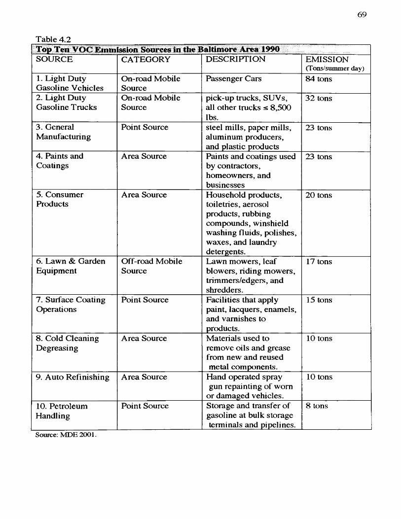
69
Table 4.2isslon Sources in the Itaitimwe Area 1990
SOURCE CATEGORY DESCRIPTION EMISSION(Tons/summer day)
1, Light Duty Gasoline Vehicles
On-road Mobile Source
Passenger Cars 84 tons
2. Light Duty Gasoline T rucks
On-road Mobile Source
pick-up trucks, SUVs, all other trucks ^ 8,500 lbs.
32 tons
3. General Manufacturing
Point Source steel mills, paper mills, aluminum producers, and plastic products
23 tons
4. Paints and Coatings
Area Source Paints and coatings used by contractors, homeowners, and businesses
23 tons
5. Consumer Products
Area Source Household products, toiletries, aerosol products, rubbing compounds, winshield washing fluids, polishes, waxes, and laundry detergents.
20 tons
6. Lawn & Garden Equipment
Off-road Mobile Source
Lawn mowers, leaf blowers, riding mowers, trimmers/edgers, and shredders.
17 tons
7. Surface Coating Operations
Point Source Facilities that apply paint, lacquers, enamels, and varnishes to products.
15 tons
8. Cold Cleaning Degreasing
Area Source Materials used to remove oils and grease from new and reused metal components.
10 tons
9. Auto Refinishing Area Source Hand operated spray gun repainting of worn
or damaged vehicles.
10 tons
10. Petroleum Handling
Point Source Storage and transfer of gasoline at bulk storage terminals and pipelines.
8 tons
Source: MDE 2001.
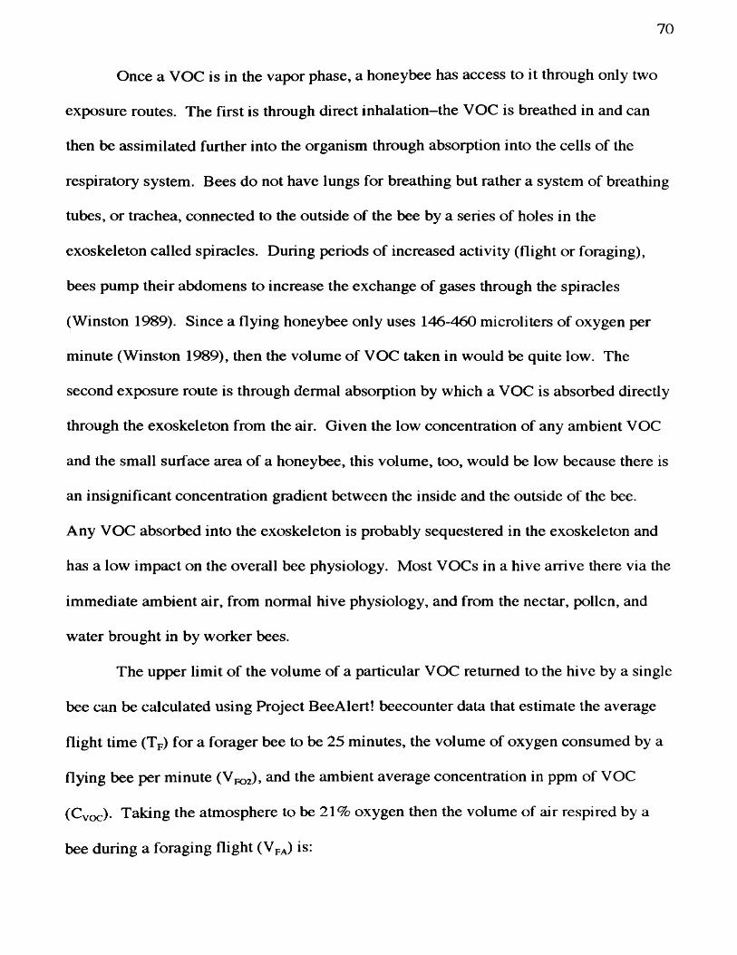
70
Once a VOC is in the vapor phase, a honeybee has access to it through only two
exposure routes. The first is through direct inhalation-the VOC is breathed in and can
then be assimilated further into the organism through absorption into the cells of the
respiratory system. Bees do not have lungs for breathing but rather a system of breathing
tubes, or trachea, connected to the outside of the bee by a series of holes in the
exoskeleton called spiracles. During periods of increased activity (flight or foraging),
bees pump their abdomens to increase the exchange of gases through the spiracles
(Winston 1989). Since a flying honeybee only uses 146-460 microliters of oxygen per
minute (Winston 1989), then the volume of VOC taken in would be quite low. The
second exposure route is through dermal absorption by which a VOC is absorbed directly
through the exoskeleton from the air. Given the low concentration of any ambient VOC
and the small surface area of a honeybee, this volume, too, would be low because there is
an insignificant concentration gradient between the inside and the outside of the bee.
Any VOC absorbed into the exoskeleton is probably sequestered in the exoskeleton and
has a low impact on the overall bee physiology. Most VOCs in a hive arrive there via the
immediate ambient air, from normal hive physiology, and from the nectar, pollen, and
water brought in by worker bees.
The upper limit of the volume of a particular VOC returned to the hive by a single
bee can be calculated using Project BeeAlert! beecounter data that estimate the average
flight time (Tp) for a forager bee to be 25 minutes, the volume of oxygen consumed by a
flying bee per minute (Vpoj), and the ambient average concentration in ppm of VOC
(Cvoc)- Taking the atmosphere to be 21% oxygen then the volume of air respired by a
bee during a foraging flight (VpJ is:
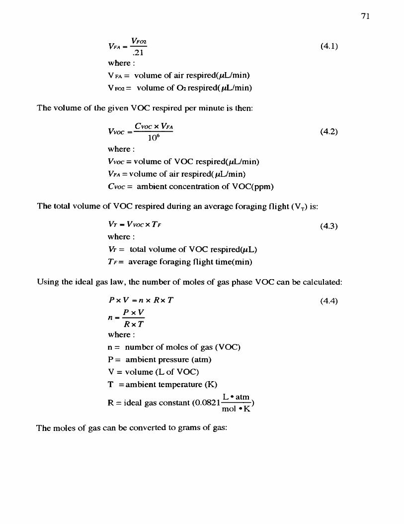
71
(4.1).21
where :V f a = volume of air respired(juL/min)V F0 2 = volume of O2 respired( /iL/min)
The volume of the given VOC respired per minute is then:
Vvoc = --------- (4.2)Cvoc X V f a
10 where :Vvoc = volume of VOC respired(juL/min)V f a = volume of air respired( L/min)Cvoc = ambient concentration of VOC(ppm)
The total volume of VOC respired during an average foraging flight (V-r) is:
V t = V VOC x T f (4.3)where :V t = total volume of VOC respired(juL)T f = average foraging flight time(min)
Using the ideal gas law, the number of moles of gas phase VOC can be calculated:
P x V =n X R x T (4.4)P x V n --------R x T
where :n = number of moles of gas (VOC)P = ambient pressure (atm)V = volume (L of VOC)T = ambient temperature (K)
R = ideal gas constant (0.0821 ^ )mol «K
The moles of gas can be converted to grams of gas:
72
( 4 .5 )n
Mvoc SB = n X MM where :Mvoc SB = mass of VOC (g) brought in by a single bee per trip MM = molar mass (g/mol) n = number of moles of gas g = number of grams of gas
Taking the ambient concentrations of benzene (MM=78.11) to be 4.6 ppm, of TCE
(MM=131.40) to be .22 ppb, and of styrene (MM=104.14) to be .01 ppm (Seinfeld 1998),
ambient pressure to be 1 atm, and ambient temperature to be 298 K, a single bee on an
average 25 minute foraging flight could respire between 2.39 x 10' g and 8.05 x 10 g
benzene, 2.05 x 10 “ g and 6.45 x 10 “ g TCE, and 7.41 x 10“® g and 2.33 x 10* g
styrene. These are extremely small amounts.
These calculations can be expanded to estimate the upper limit of the total amount
of a VOC a hive could potentially experience via the cummulated foraging of all the
foraging bees. A strong nucleus hive has approximately 10,000 foraging bees
(Bromenshenk 2001). Estimates of the number of foraging trips a single bee takes per
day varies widely but ten per day is well accepted (Winston 1989). As many as 29 pollen
loads in a day, 150 trips to artificial syrup dishes, and 110 water trips in a day have been
observed (Winston 1989). Using these estimates the total mass of a VOC entering a hive
per day is:
73
Mvoc = Mvoc SB X Nft X Nfb (4.6)where :Mvoc = Mass (g) of VOC entering hive per day Mvoc SB = mass of VOC (g) brought in by a single bee per trip N f t = average number of foraging trips per day = 10 Nfb = number of foraging bees per hive - 10
The masses of VOC calculated above can then be used to calculate a predicted
hive concentration if the total mass is assumed to revolatalize once in the hive.
The estimated volume of air in a nucleus hive is approximately 5 L. Using the
u- A 1 P1 XV1 P2 XV2combined gas law : --------- = --------------------- (4.7)Ti T2
and an average hive temperature of 35 °C (308 K), the molar volume of a gas can be
derived as 25.3 L. The number of gas (air) molecules in the hive is then:
N Air — V hive X Vmolar gas X N avagadro
where :N Air = number of air molecules in hive Vhive = 5 L Vmolar gaa — 25.3 L/mol N avagadro = 6.02 X 10^ molecules/mole
The number of VOC molecules brought in by the hive in one day is then:
Nvoc = Mvoc X MMvOC ' X NAvagodro (4 9)where :Nvoc = number of VOC molecules entering hive per day Mvoc = Mass (g) of VOC entering hive per day MM VOC = molar mass of the VOC (g/mol)
The concentration in ppt is then:
74
Cvoc= ^ x i o "N Air
where ;Cvoc = concentration o f VOC in ppt
Using these calculations described above, the predicted maximum concentrations
are:
Benzene 1.55 x 10 ® to 5.21 x 10 ® ppt.
TCE 7.89 X 10 to 2.48 x 10 ppt.
Styrene 3.60x 10’ to 1.13 x 10® ppt.
These calculated concentrations are all well above the measured hive concentrations for
several reasons. These calculations also assumed that all VOC taken in during flight will
be reemitted in the hive. Assuming that the individual bee retains 100% of the respired
VOC during flight and then exhales 100% of that volume once returned to the hive is
unrealistic. In fact there is an equilibrium partition gradient that resists both the inflight
retention and the in hive exhalation. These calculations also have not taken into account
the dynamic air circulation in the hive. During the summer the hive covers are propped
open to permit evaporative cooling as needed by the colony. The resultant air circulation
will cause dissipation of the in coming contaminants. Finally the various materials in the
hives are absorbent and could complex the compounds further removing them.
If the VOC is absorbed to the surface of airborne particulate, then the exposure
route could be broadened. The particulate could be respired through the spiracles and
further assimilated as if it were inhaled. In another scenario the particulate could become
attached to a micro hair of the bee through electrostatic attraction and the VOC could be
absorbed through the exoskeleton, or combed into the pollen pellet and later ingested, or
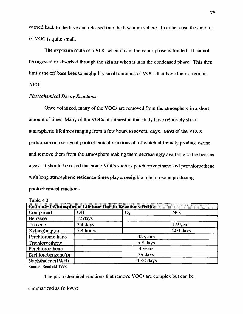
75
carried back to the hive and released into the hive atmosphere. In either case the amount
of VOC is quite small.
The exposure route of a VOC when it is in the vapor phase is limited. It cannot
be ingested or absorbed through the skin as when it is in the condensed phase. This then
limits the off base bees to negligibly small amounts of VOCs that have their origin on
APG.
Photochemical Decay Reactions
Once volatized, many of the VOCs are removed from the atmosphere in a short
amount of time. Many of the VOCs of interest in this study have relatively short
atmospheric lifetimes ranging from a few hours to several days. Most of the VOCs
participate in a series of photochemical reactions all of which ultimately produce ozone
and remove them from the atmosphere making them decreasingly available to the bees as
a gas. It should be noted that some VOCs such as perchloromethane and perchloroethene
with long atmospheric residence times play a negigible role in ozone producing
photochemical reactions.
Table 4.3Estimated Atmospheric Lifetime Due to Reactions With:Compound OH O3 NO3
Benzene 1 2 daysToluene 2.4 days 1.9 yearXylene(m,p,o) 7.4 hours 2 0 0 daysPerchloromethane 42 yearsT richloroethene 5-8 daysPerchloroethene 4 yearsDichlorobenzene(p) 39 daysNaphthalene(PAH) .4-40 daysSource; Seinfeld 1998.
The photochemical reactions that remove VOCs are complex but can be
summarized as follows:
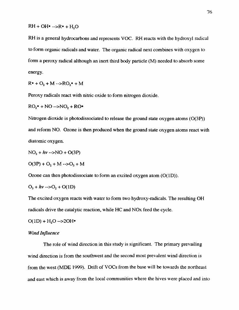
76
RH + OH* ->R* + HjO
RH is a general hydrocarbons and represents VOC. RH reacts with the hydroxyl radical
to form organic radicals and water. The organic radical next combines with oxygen to
form a peroxy radical although an inert third body particle (M) needed to absorb some
energy.
R* + O2 + M ->R02* + M
Peroxy radicals react with nitric oxide to form nitrogen dioxide.
RO2* + NO ->N02 + RO*
Nitrogen dioxide is photodissociated to release the ground state oxygen atoms (0(3P))
and reform NO. Ozone is then produced when the ground state oxygen atoms react with
diatomic oxygen.
NO2 + hv —>NO + 0(3P)
0(3P) + O2 + M - > 0 3 + M
Ozone can then photodissociate to form an excited oxygen atom (0(1D)).
O3 + hv - > 0 2 + 0(1D)
The excited oxygen reacts with water to form two hydroxy-radicals. The resulting OH
radicals drive the catalytic reaction, while HC and NOx feed the cycle.
0(1D) + H2O ->20H*
Wind Influence
The role of wind direction in this study is significant. The primary prevailing
wind direction is from the southwest and the second most prevalent wind direction is
from the west (MDE 1999). Drift of VOCs from the base will be towards the northeast
and east which is away from the local communities where the hives were placed and into
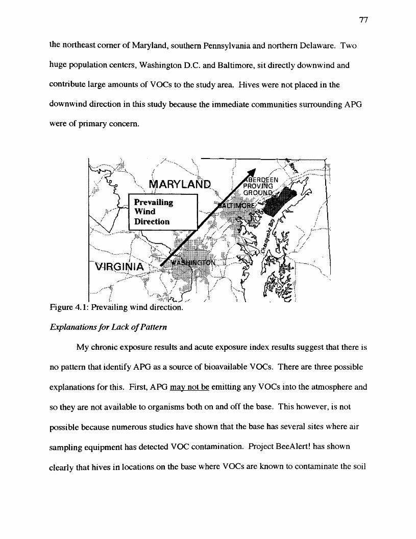
77
the northeast comer of Maryland, southern Pennsylvania and northern Delaware. Two
huge population centers, Washington D.C. and Baltimore, sit directly downwind and
contribute large amounts of VOCs to the study area. Hives were not placed in the
downwind direction in this study because the immediate communities surrounding APG
were of primary concern.
I IARYLANmPrevailingWindDirection
Figure 4.1: Prevailing wind direction.
Explanations for Lack o f Pattern
My chronic exposure results and acute exposure index results suggest that there is
no pattern that identify APG as a source of bioavailable VOCs. There are three possible
explanations for this. First, APG may not be emitting any VOCs into the atmosphere and
so they are not available to organisms both on and off the base. This however, is not
possible because numerous studies have shown that the base has several sites where air
sampling equipment has detected VOC contamination. Project BeeAlert! has shown
clearly that hives in locations on the base where VOCs are known to contaminate the soil
78
and water also have elevated levels of VOCs in the hive atmosphere, as well as elevated
ambient VOC levels.
Second, the base may be a source of VOCs but the downwind Washington D.C.
and Baltimore Metropolitan areas, which also emit VOCs, as well as numerous local
point sources are overwhelming the detectable pattern. Soil vapor releases do not
transport very well, and there are no stacks on APG as an emission source. The only
stacks near APG are at a non-APG waste-to-energy plant near the northwestern Magnolia
Gate entrance, and at a coal fired power plant near Carroll Island, which is to the west of
the Gunpowder Neck. The on-base labs could be a source of VOCs but those emissions
are likely small and would result in no aerosol entrainment.
Third may be flaws in the study design that prevent the pattern from being
detected. It could be there are too few hives for such a large area and the sampling
interval is too long given the demonstrated short hive retention time for VOCs.
ANOVA Trends
Several trends that emerge from the ANOVA are disussed here. The ANOVA
trends shed some light on the influences of urban areas on VOC concentrations.
For the PC-1 (gasoline components) there is elevated variation at Zone 3 and on
Heading 1, which is the Rumsey Mansion sampling site, and Zones 9 and 21 on Heading
2, which are the Towerhill and Farview Manor sampling sites, respectively. This
variation is greater in the month of September than it is in July. Two of these sites,
Rumsey Mansion and Towerhill, are directly downwind from the Baltimore Metropolitan
area. Since PC-1 is heavily weighted with gasoline components it is possible that the
variation has its origin in a plume of VOCs emitted from the city. The elevated variation
79
at Farview Manor is probably rooted in the agricultural activity in the area, since the
hives are physically located within a landscaping and nursery business, which is adjacent
to a gas station. However, the Silverlake Drive sampling site, which also sits in the
middle of the downwind plumes, shows no variation in the PC-1. This site suggests the
plume may not be the single most important source.
A notable trend to emerge from the ANOVA is that the least amount of variation
is assignable to the treatment-whether the sample was collected from the hive or ambient
air. This has ramifications for a study that uses honeybees to determine the
bioavailability of VOCs that are regionally dispersed. Since the boundary study airshed
is dominated by ubiquitous BTEX components it is not surprising that ambient and hive
levels exhibited similar patterns. If the hive air is not statistically different from the
ambient air with respect to VOCs concentrations, then why expend significant resources
in deploying and maintaining hives to monitor air quality?
While hive air samples did not prove useful for improving measurements of
regional, low concentration, vapor phase VOCs, they did provide evidence for a local
“hotspot”. PC-4, an inverse relationship between benzene and perchloroethene, and
dichloromethane and toluene, shows elevated variation in Zone 9, Heading 1, which is
the Silverlake Drive site. The variation is entirely in the month of July rather than
September as it was in PC-1. This suggests that the Silverlake Drive area is a “hotspot”
for a hazardous air pollution source other than disperse regional sources such as
automobile emissions, emissions from chlorinated swimming pools, or emissions from
drinking water treatment facilities.
80
Hive samples have proven to be effective at elucidating contaminant plumes in
the past. In a similar study conducted in the Upper Snake River Plain of Idaho, hives
were used to monitor atmospheric flouride. In this study three industrial sources of
flouride were identified and flouride distribution from anthropogenic and natural sources
were mapped. The study established a clear concentration gradient of flouride from one
of the industrial sources - a phosphate ore processing facility - and established it and not
the other two industrial sources as the dominant regional flouride source across an area
comparable in size to the APG boundary study area (Bromenshenk et al. 1996).
There are two main differences between the Idaho study and this Maryland study.
First, the sources of flouride in Idaho were known point sources and the Maryland study
investigated non-point sources. Second, flouride is relatively stable in the semi-arid
environment of the Snake River Plain being most suseptible to degradation in wet
environments (Connel and Miller 1984), and the VOCs studied in Maryland are often
easily degraded in physiologically related pathaways. These differences probably have
influenced the lack of variation between hive and air samples in this study.
Despite the results of this study, 1 believe honeybees are still extremely useful
monitors of environmental contaminants. They monitor the environment continuously,
are multimedia samplers, and assess synergistic effects of all enviromental contaminants.
Systematic monitoring studies rely upon regularly scheduled sampling at a
specific location. These periodic “grab” samples usually miss acute VOC releases.
Honeybees are continuous samplers. They sample a mile wide area, 24 hours a day, 7
days a week during the spring through fall foraging season. An acute release of a VOC
within an area may not be detected in a weekly or monthly ambient air sample but may
81
be “recorded” in the hive as a change in the overall health of the colony or retained in the
stored hive resources (honey, propolis, and pollen).
In addition, honeybees are multimedia samplers. Bee hives are living systems
whose viability is a function of the quality of the environment. Hives integrate many
media exposure routes from all media (air, water, soil, and vegetation) and assess the
effect of all contaminants whether or not a compound is included in an investigation’s
“hit list.” Our study was limited to sampling only one media at a time (air) and our
routine analysis quantified only 54 of the millions of potential chemical exposures.
Honeybees assess the synergistic impacts from a mixture of contaminants
whereas periodic sampling of the area cannot accomplish this. Synergistic impacts - the
increased sensitivity to chemical A by the action of chemical B - can result from
exposure to multiple chemicals in the environment including VOCs, SVOCs, PAHs,
heavy metals, and radioactive materials. Combinations of two or several chemicals can
influence the hive physiology and cause measurable changes such as population decrease,
or loss of a laying queen. No systematic analysis of a “hit list” can yield a better metric
of the cumulative impact of environmental contaminants to living systems.
Conclusions
The focus of this study was to determine if APG is a source of regionally
bioavailable VOCs by utilizing techniques developed by Project BeeAlert!. Although
other Project BeeAlert! studies identified areas on APG where VOCs are available to
honeybees, this study concludes that APG is not a source of bioavailable VOCs based
upon our sampling of the area in summer and fall of 1998 and 1999, and the three
different data reduction techniques employed to analyze the data. This conclusion is
82
plausible for three reasons: First, there is no pattern that suggests APG is a source (i.e., a
concentration gradient that falls as distance is gained from the base), nor is there any
discernible pattern where the ambient air is higher or lower than hive air. This may be
due in part to fluctuations in weather patterns and/or the volatile nature of the
contaminants studied. Second, the Acute Exposure Index suggests that sites where high
VOC concentrations are in both the ambient air and the hive air are also sites where
human activity (particularly vehicle traffic) influences the available VOCs. We cannot
associate these high hits with a release event on the base itself. Third, analysis of
variance shows that the variation in chemistry is a function of season to a large extent and
distance and direction to a lesser extent. Very little variation in chemistry exists between
the hive air and ambient air. There is no pattern of variation that suggests the base is a
source of contaminants.
This study may have demonstrated some limitations of using honeybees as
environmental samplers. Bees are certainly useful for determining acute toxicity
chemicals such as pesticides, and of determining the bioavailability of metals, nonmetals
and radioactive materials. They are good for local “hot spot” VOC assessment where no
stack source is present. Bees have also been successfully used to determine the
bioavailability of VOCs as long as the source is non-vapor phase. Significant differences
in hive chemistry and viability were seen in O-Field before and after a clean-up. In this
study beehives did not prove useful for detecting bioavailability of regional VOCs when
they were at low concentrations and in the vapor phase only.
83
Suggestions for Further Study
Much uncertainty still exists in the source and transport of VOCs in northeast
Maryland- Ideally, researchers could repeat this study with the following changes. First,
a mile-by-mile grid could be overlaid on the study area and paired hives could be placed
at sites as close to the center of the grid squares as possible. This would guarantee an
unbroken coverage of the landscape since one mile approximates the area over which a
normal hive will forage. Increased coverage would improve the resolution and
magnitude of “hotspot” areas such as Silverlake Drive. Second, the study area could be
extended to include downwind communities and locations (northeast and east of APG)
allowing us to see APG leaks or regular emissions. Third, the hives and air could be
sampled every two weeks beginning in early spring and continuing through the fall.
Extra samples could be taken if MDE monitors suggest the formation of abnormal
plumes. This sampling should cover the entire foraging season enabling researchers to
track contributions from changing vegetation. Acute release events could be monitored
so we can better understand their fate. Finally, systematic replicate samples for each hive
and ambient air should be taken. A researcher could easily put two Swagelok T’s in the
sample train of the JAG Box and split the flow such that air was pulled through two
sample tubes in tandem. This would significantly improve the QA/QC in the study.
The draw back to the above suggestions is the expense. The suggested study
would generate a huge volume of samples for analysis as well as require a fulltime crew
to do the hive maintenance and sampling. The benefit of such a study would be a very
clear picture of the distribution and bioavailability of VOCs in the area.
84
REFERENCES
Alnasser, G. H. 1998. The Use of Thermal Desorption/Gas Chromatography/Mass
Spectrometry (TD/GC/MS), Honey Bees, and Artificial Neural Networks
(ANN) in Assessing Ecosystem Contamination. Ph.D. Thesis. Missoula:
University of Montana.
American Conference of Governmental Industrial Hygienists. 1995. 1995-1996
Threshold Limit Values (TLVs) for Chemical Substances and Physical Agents
and Biological Exposure Indices (BEIs). Cincinnati, Ohio: ACGIH.
Argonne (Argonne National Laboratory) 1998. Remedial Investigation Report for
J-FieId, Aberdeen Proving Ground, Maryland, Vol. 1, Remedial Investigation
Results, Draft-Final. June 1998.
Bankova, V. S., Popov, S. S. and Marekov, N. L. 1982. High-performance liquid
chromatographic analysis of flavonoids from propolis. Journal of Chromatography 242(1): 135-143.
Bankova, V. S., Popov, S. S. and Marekov, N. L. 1989. Isopentenyl cinnamates
from poplar buds and propolis. Phytochemistry 28(3):871-873.
Bromenshenk, J. J., 1998. Research Professor and Director Project BeeAlert!,
University of Montana, Missoula, Montana, personal communication.
Bromenshenk, J. J, Cronn, R. C., Nugent, J. J. 1992. Surveillance monitoring of
the Idaho National Engineering Laboratory with honey bees. In Ecological
Indicators, McKenzie, D. H.,Hyat, E. D., McDonald, V. J., Eds., Elsevier
Science: London, 1992, Vol. 2, 1522-1523.
Bromenshenk, J. J, Cronn, R. C., Nugent, J. J. 1996. Monitoring Flouride with
Honey Bees in the Upper Snake River Plain of Idaho. Journal of
Environmental Quality 25(4):868-877.
Bromenshenk, J. J., Smith, G. C. and Watson, V. J. 1995. Assessing ecological risks in
terrestrial systems with honey bees. Environ. Sci. Res. 50:9-30.
Bromenshenk, J. J., Smith, G. C., King, B. E., Seccomb, R. A., Jones, D. C., Taylor, M,
Henderson, C. H., Alnasser, G. H. and Wrobel, C. L. 1999. Aberdeen Proving
Ground Bee Studies: New and Improved Methods for Monitoring Air Quality and the
85
Terrestrial Environment: Applications at Aberdeen Proving Ground—Edgewood
Area. Annual Research and Interim Project Report. U.S. Army Center for
Environmental Health Research, Ft. Detrick, Md. USA Contract DAMA 17-95-C-
5072.
Bromenshenk, J. J., Smith, G. C., King, B. E., Seccomb, R. A., Alnasser, G. H.,
Loeser, M. R.; Henderson, C. B. and Wrobel, C. L. 1998. New and Improved
Methods for Monitoring Air Quality and the Terrestrial Environment:
Applications at Aberdeen Proving Ground—Edgewood Area. Annual Report,
1998. U.S. Army Center for Environmental Health Research, Ft. Detrick, Md.
USA Contract DAMA 17-95-C-5072.
Bromenshenk, J. J., Smith, G. C., Seccomb, R. A., King, B. E., Alnasser, G. H.,
Henderson, C. B. and Wrobel, C. L. 1997. New and Improved Methods for
Monitoring Air Quality and the Terrestrial Environment. Annual Report,
1997. U.S. Army Center for Environmental Health Research, Ft. Detrick, Md.
USA Contract DAMA 17-95-C-5072.
Burgess, J. H., Bromenshenk, J. J., Jones, D. C., 2000. Work plan and analysis
protocols for monitoring o f exposures to bioavailable contaminants at J-field,
Edgewood area, Aberdeen Proving Ground, Maryland. Prepared by Roy F.
Weston, Inc. and University of Montana for Directorate of Safety, Health and
Environment. U.S. Department of the Army.
Burken, J. G. and Schnoor, J. L. 1998. Predictive relationships for uptake of
organic contaminants by hybrid poplar trees. Environ. Sci. Technol.
32:3379-3385.
Christian, T. J. 1996. Analysis of polychlorinated biphenyls in honey bees.
Master’s Thesis. Missoula: University of Montana.
Connell, D. W. and Miller G. J. 1984. Chemistry and Ecotoxicology of Pollution.
John Wiley and Sons, Inc., New York. pp. 350-355.
Edgerton, S. A., Khalil, M. A. and Rasmussen, R. A. 1986. Source emission
characterization of residential wood-burning stoves and fireplaces. Environ.Sci. Technol. 20:803-807.
86
Harris, D. C. 1995. Quantitative Chemical Analysis, 4* Edition, New York: W. H.
Freeman and Company, pp. 655-692.
Henderson, Colin B. 2001, personal communication.
Hiatt, M. H. 1999. Leaves as an indicator of exposure to airborne volatile organic
compounds. Environ. Sci. Technol. 33:4126—4133.
Komp, P. and McLachlan, M. S. 1997. Influence of temperature on the plant/air
partitioning of semivolatile organic compounds. Environ. Sci. Technol.
31(3):886-890.
Lee, L. S., Hagwall, M., Delfino, J. J., Rao, P. S. C. 1992. Partitioning of
polycyclic aromatic hydrocarbons from diesel fuel into water. Environ. Sci.
Technol. 26:2104-2109.
Markham, K. R., Mitchell, K. A., Wilkins, A. L., Daldy, J. A. and Lu, Y. 1996.
HPLC and GC-MS identification of the major organic constituents in New
Zealand propolis. Phytochemistry 42(1):205-211.
Martos, I., Cossentini, M., Ferreres, F. and Tomâs-Barberân, F. A. 1997.
Flavonoid composition of Tunisian honeys and propolis. J. Agric. Food Chem. 45:2824-2829.
Morse, R. A., and Hooper, T. 1985. The Illustrated Encyclopedia o f Beekeeping.
New York: E. P. Dutton, Inc.
Middleton, P. 1995. Sources of air pollutants, in Composition, Chemistry, and
Climate o f the Atmosphere, Singh, H. B., editor. Van Nostrand Reinhhold,
New York, pp. 88-119.
National Research Council. 1991. Animals as Sentinels o f Environmental Health
Hazards. Washington D. C., National Academy Press.
Nemeth, G. 1989. RCRA Facility Assessment, Edgewood Area, Aberdeen Proving
Ground, Maryland. U.S. Army Environmental Hygiene Agency, Waste
Disposal Engineering Division, Aberdeen Proving Ground, MD. November
1989.
Newman, L. A., Strand, S. E., Choe, N., Duffy, J., Ekuan, G., Ruszaj, M.,
Shurtleff, B. B., Wilmoth, J., Heilman, P. and Gordon, M. P. 1997. Uptake
87
and biotransformation of trichloroethylene by hybrid poplars. Environ. Sci.
Technol. 31:1062—1067.
Patte, F., Etcheto, M., Marfaing, P. and Laffort, P. 1989. Electroantennogram
stimulus-response curves for 59 odourants in the honey bee. Apis mellifica. J. Insect Physiol. 35(9):667-675.
Pereira, A. S., Pinto, A. C., Cardoso, J. N. and Aquino Neto, F. R. 1998.
Application of high temperature resolution gas chromatography to crude
extracts of propolis. J. High Resol. Chromatogr. 21:396-400.
Placet, M., Battye, R. E., Fehsenfeld, F. C., Bassett, G. W. 1990. Emmissions
involved in Acidic Deposition Processes. State-of-Science/Technology Report
1. National Acid Precipitation Assessment Program. U. S. Government
Printing Office,Washington, D. C.
Rogge, W. F., Hildemann, L. M., Mazurek, M. A. and Cciss, G. R. 1997. Source
of fine organic aerosol. 8 . Boilers burning No. 2 distillate fuel Oil. Environ. Sci. Technol. 31:2731-2737.
Russell, J. W. 1975. Analysis of air pollution using sampling tubes and gas
chromatography. Environ. Sci. Technol. 9:1175-1182.
Sakuma, H., Munakata, S. and Sugawara, S. 1981. Volatile products of cellulose
pyrolysis. Agri. and Biol. Chem. J. 45:443-451.
Seinfeld, J. H., Pandis, S. N., 1998 Atmospheric Chemistry and Physics. New
York. John Wiley and Sons, Inc. pp. 49-116.
Sigman, M. E., Guerin, M. R., Smith, G. C. and ligner, R. H. 1998. Sol-Gel
Sorbents. In Proceedings o f the First Conference on Engineered Bee
Colonies, DARPA, Controlled Biological Systems (Bromenshenk, J. J., ed.)
Missoula: University of Montana, pp. 10-17.
Singh, H. B., Salas, L., Viezee, W., Sitton, B. and Ferek, R. 1992. Measurement
of volatile organic chemicals at selected sites in California. Environment
26A(16):2929-2946.
Smith, G. C. and Wrobel, C. L. 1998. Neural networks in industrial and
environmental applications. In Soft Computing in Systems and Control
88
Technology, (Tzafestas, S. G. ed.) Hong Kong: World Scientific Press, pp.
445-466.Smith, G. C., Bromenshenk, J. J., Jones, D. C., Alnasser, G. H. 2001. Volatile and
semi-volatile organic compounds in beehive atmospheres, in Estimating the
Environmental Impacts of Chemicals to Honeybees. Devillers, J., Pham-
Delegue, M. H. Eds, in press.
State of Maryland Air and Radiation Management Administration, Division of
Air Monitoring, 1999. Maryland Air Quality Data Report 1999.
Thompson, P. L., Ramer, L. A. and Schnoor, J. L. 1998. Uptake and
transformation of TNT by hybrid poplar trees. Environ. Sci. Technol.32:975-980.
Tulloch, A. P. 1980. Beeswax composition and analysis. Bee World 61:47-62.
U.S. Environmental Protection Agency. 1999. Compendium of Methods for the
Determination o f Toxic Organic Compounds in Ambient Air. Second Edition.
Office of Research and Development.
UATW, Unified Air Toxics Website, U.S. EPA, 1998.
http://www.epa.gov/ttn/uatw/hapindex.html
Warren-Hicks, W., Parkhurst, B. R. and Baker, S. S., Jr. 1989. Ecological Assessments of
Hazardous Waste Sites. U.S. Environmental Protection Agency 600/3-89/013.
Westerholm, R. and Egeback, K-E. 1994. Exhaust emissions from light-and
heavy-duty vehicles. Environ. Health Perspec. 102:13-23.
Westerholm, R. and Li, H. 1994. A multivariate analysis of fuel-related polycyclic
aromatic hydrocarbon emissions from heavy-duty diesel vehicles. Environ.
Sci. Technol. 28:965-972.
Winston, M. L. 1987. The Biology o f the Honey Bee. Cambridge, Mass.: Harvard
University Press.
Woolfenden, E. 1997. Monitoring VOCs in air using sorbent tubes followed by
thermal desorption-capillary GC analysis: Summary of data and practical
guidelines. J. Air & Waste Manage. Assoc. 47:20-36.
89
Wrobel, C. L., 2000. Investigating Volatile Organic Compounds in an Urban
Inter-Mountain Valley Using a TD/GC/MS Methodology and Intrinsic Tracer
Molecules. PhD. Thesis. Missoula: University of Montana.
Zhang, X. J. and Peterson, F. 1996. Emissions from co-combustion of wood
household refuse. Waste Renew, Energy Comb, 9:997-1000.
90
APPENDIX A: Sampling Protocol for VOC from Beehives
Equipment
JAG Box assembly:Weather proof container-Rubbermaid^“ servin’saver 710 ml food storage container.
Tubing: 1/8 inch O.D. cleaned copper.Connectors: Swagelok™
Ix tubing to 1/4” union,3x 1/8” to 1/4” union,2x 1/8” to 3/8 union.
Sorbtion Tubes:Ix Supelco carbotrap 400,Ix Supelco carbotrap 150,72150881X SKC drying tube packed with 9000 mg of anhydrous sodium sulfate
(Model 226-44-02).
Air Sampling Pump: SKC Personal Air Sampler (Model 222-3)
Connector Tubing: 1 meter length Tygon® R-3603 tubing 3/161.D.; 30 cm length of 1/8l.D. Tygon® tubing
Calibration Row Meter:
Battery powered drill and 3/16 wood drilling bit.
Small flat blade screw driver
Sampling Log Sheet and adhesive sample labels.
l ”x l” squares of aluminum foil
Stainless steel airtight coffee storage container.
Igloo ice chest with triple bagged ice.
Settings
Sampling Row Rate: 100.0 ml/min +/- 2.0 ml/min
Sampling Time: Approximately 8 hours
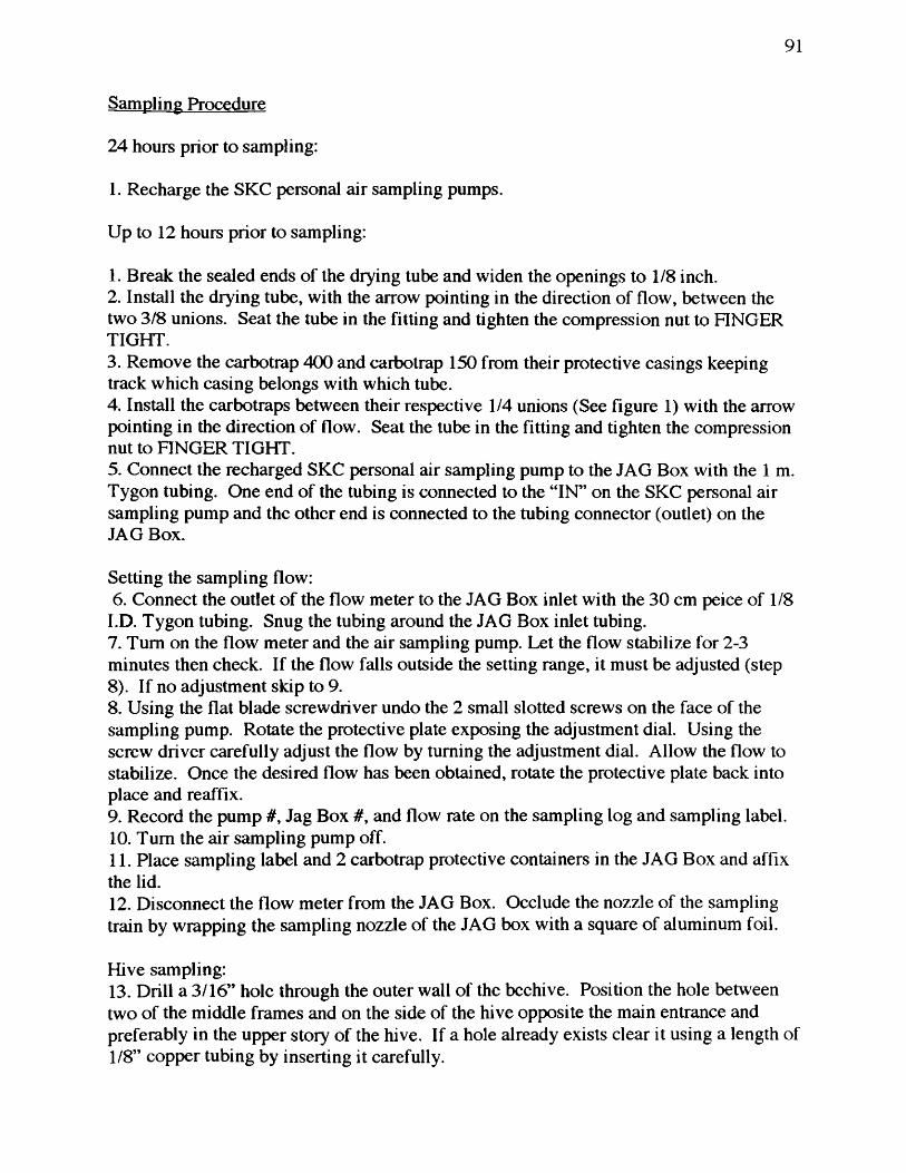
91
Sampling Procedure
24 hours prior to sampling:
1. Recharge the SKC personal air sampling pumps.
Up to 12 hours prior to sampling:
1. Break the sealed ends of the drying tube and widen the openings to 1/8 inch.2. Install the drying tube, with the arrow pointing in the direction of flow, between the two 3/8 unions. Seat the tube in the fitting and tighten the compression nut to FINGER TIGHT.3. Remove the carbotrap 400 and carbotrap 150 from their protective casings keeping track which casing belongs with which tube.4. Install the carbotraps between their respective 1/4 unions (See figure 1) with the arrow pointing in the direction of flow. Seat the tube in the fitting and tighten the compression nut to FINGER TIGHT.5. Connect the recharged SKC personal air sampling pump to the JAG Box with the 1 m. Tygon tubing. One end of the tubing is connected to the “IN” on the SKC personal air sampling pump and the other end is connected to the tubing connector (outlet) on the JAG Box.
Setting the sampling flow:6 . Connect the outlet of the flow meter to the JAG Box inlet with the 30 cm peice of 1/8
l.D. Tygon tubing. Snug the tubing around the JAG Box inlet tubing.7. Turn on the flow meter and the air sampling pump. Let the flow stabilize for 2-3 minutes then check. If the flow falls outside the setting range, it must be adjusted (step 8 ). If no adjustment skip to 9.8 . Using the flat blade screwdriver undo the 2 small slotted screws on the face of the sampling pump. Rotate the protective plate exposing the adjustment dial. Using the screw driver carefully adjust the flow by turning the adjustment dial. Allow the flow to stabilize. Once the desired flow has been obtained, rotate the protective plate back into place and reaffix.9. Record the pump #, Jag Box #, and flow rate on the sampling log and sampling label.10. Turn the air sampling pump off.11. Place sampling label and 2 carbotrap protective containers in the JAG Box and affix the lid.12. Disconnect the flow meter from the JAG Box. Occlude the nozzle of the sampling train by wrapping the sampling nozzle of the JAG box with a square of aluminum foil.
Hive sampling:13. Drill a 3/16” hole through the outer wall of the beehive. Position the hole between two of the middle frames and on the side of the hive opposite the main entrance and preferably in the upper story of the hive. If a hole already exists clear it using a length of 1 /8 ” copper tubing by inserting it carefully.
92
14. Remove the aluminum foil from the nozzle and insert the nozzle end of the sampling train of the JAG box into the hole so the tip of the nozzle is midway into the hive.
15. Turn the sampling pump on and record the start time and hive # information.
16. After 6 - 8 hours return to retrieve the sample.
17. Upon return remove the nozzle from the hive and attach the flow meter. After the flow has stabilized record the flow.
18. Switch the pump off and remove the air flow meter. Record the stop time.
19. Immediately remove the Carbotrap 400 sample tube and place it in its protective case. Affix the sample label to the outside of the protective covering. The sample is then placed in the airtight stainless steel container. Place the airtight container in the igloo cooler with the triple bagged ice.
20. Samples are stored in a sample freezer at -5 C till shippment.
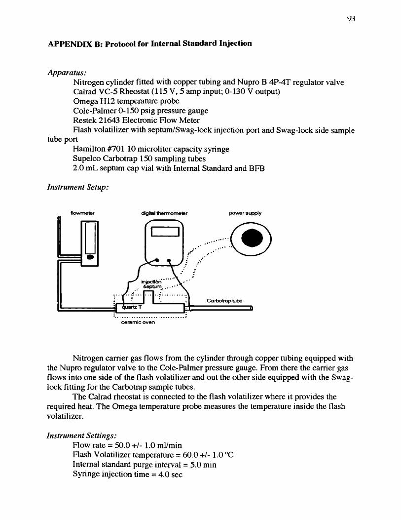
93
APPENDIX B: Protocol for Internal Standard Injection
Apparatus:Nitrogen cylinder fitted with copper tubing and Nupro B 4P-4T regulator valve Calrad VC-5 Rheostat (115 V, 5 amp input; 0-130 V output)Omega H12 temperature probe Cole-Palmer 0-150 psig pressure gauge Restek 21643 Electronic Flow MeterFlash volatilizer with septum/Swag-lock injection port and Swag-lock side sample
tube portHamilton #701 10 microliter capacity syringeSupelco Carbotrap 150 sampling tubes2.0 mL septum cap vial with Internal Standard and BFB
Instrument Setup:
flowmetsr digital thermometar power supply
quartz T
#
ceramic oven
Nitrogen carrier gas flows from the cylinder through copper tubing equipped with the Nupro regulator valve to the Cole-Palmer pressure gauge. From there the carrier gas flows into one side of the flash volatilizer and out the other side equipped with the Swag- lock fitting for the Carbotrap sample tubes.
The Calrad rheostat is connected to the flash volatilizer where it provides the required heat. The Omega temperature probe measures the temperature inside the flash volatilizer.
Instrument Settings:Flow rate = 50.0 +/- 1.0 ml/min Flash Volatilizer temperature = 60.0 +/- 1.0 ®C Internal standard purge interval = 5.0 min Syringe injection time = 4.0 sec
94
Instrument Preparation:
1. Plug in the Calrad Rheostat. Turn the knob on top until the arrow points at the indicator dots marked on the voltage scale (dots are approximately between 6-7 volts).
2. Turn on the Omega temperature probe by pressing the “on” button. The temperature needed for use is 60 with a range of +/- 1 ®C. Adjust the Calrad Rheostat as needed.
3. Turn on the nitrogen carrier gas by opening the valve on the top of the cylinder. Turn the valve counter clockwise until it is fully open and then back clockwise for one turn.
4. Adjust the flow pressure of the gas leaving the tank by turning the pressure adjustment valve located just left of opening valve. Do this until the pressure gauge reads 40 psi.
5. Turn on the nitrogen supply to the system at the Nupro switch (small green switch) located on the copper tubing. The nitrogen should now be flowing into the flash volatilization chamber (indicated by the raised level of the mercury drop in the Cole- Palmer pressure gauge located on the apparatus board).
6 . Loosen the Swag-lock fitting on the side port of the flash volatilization chamber and removing the plastic plug (caution: built up pressure may cause the plug to eject rapidly).
7. Turn on the Restek Electronic How Meter by pressing the “on” button. Press the “mode” button until the display reads F N2 (nitrogen flow).
8 . Insert an empty Carbotrap tube in the end of the plastic tubing attached to the Restek Electronic How Meter. Insert the other end of the Carbotrap tube in the side port of the flash volatilization chamber and tighten the Swag-lock fitting using the wrench. At this point the Electronic How Meter should register a value. Adjust the flow rate to 50 mL/min by turning the knob on the Cole-Palmer pressure gauge.
9. Obtain a 2.0 mL internal standard vial from the freezer. It should be labeled “Internal Standard and BFB, 100 nanograms/microliter. Find the Hamilton 10 microliter syringe labeled internal standard.
10. Arrange the Carbotrap sample tubes in order as listed on the inventory sheet. This is the order of tubes to which the internal standard should be injected. Once each tube has been injected with the internal standard, check off that sample on the inventory sheet.
95
Internal Standard Injection:Once the system has reached the proper requirements (temperature of 60 °C, flow rate
of 50 L/min, with no fluctuation in these for at least 3 minutes) it is time to start theinjection procedure. The injection procedure is as follows:
1. Insert the Carbotrap sample tube in the end of the plastic tubing attached to the Restek Electronic Row Meter oriented so that the flow arrow on the Carbotrap sample tube points into the tubing. Insert the other end of the Carbotrap sample tube in the side port of the flash volatilization chamber and tighten the Swag-lock fitting using the wrench.
2. Insert the Hamilton 10 microliter syringe into the rubber septum on the top of the internal standard vial. When inserting the needle, be sure that the syringe plunger is not fully pushed in. Remove all air bubbles from the syringe by drawing solution in and out rapidly.
3. Draw exactly 1.0 microliter into the syringe. Take the syringe out of the internal standard vial and insert it through the septum on the top port of the volatilization chamber. Insert the needle straight downward until the needle is completely in the chamber.
4. Inject the internal standard from the syringe. Wait four seconds before removing the syringe.
5. Wait five minutes before beginning the process over again on the next Carbotrap sample tube.
6 . When done injecting Carbotrap sample tubes, turn off all equipment. Replace the septum on the internal vial sample cap and return to the freezer. Place the syringe back in the box from which it was obtained.
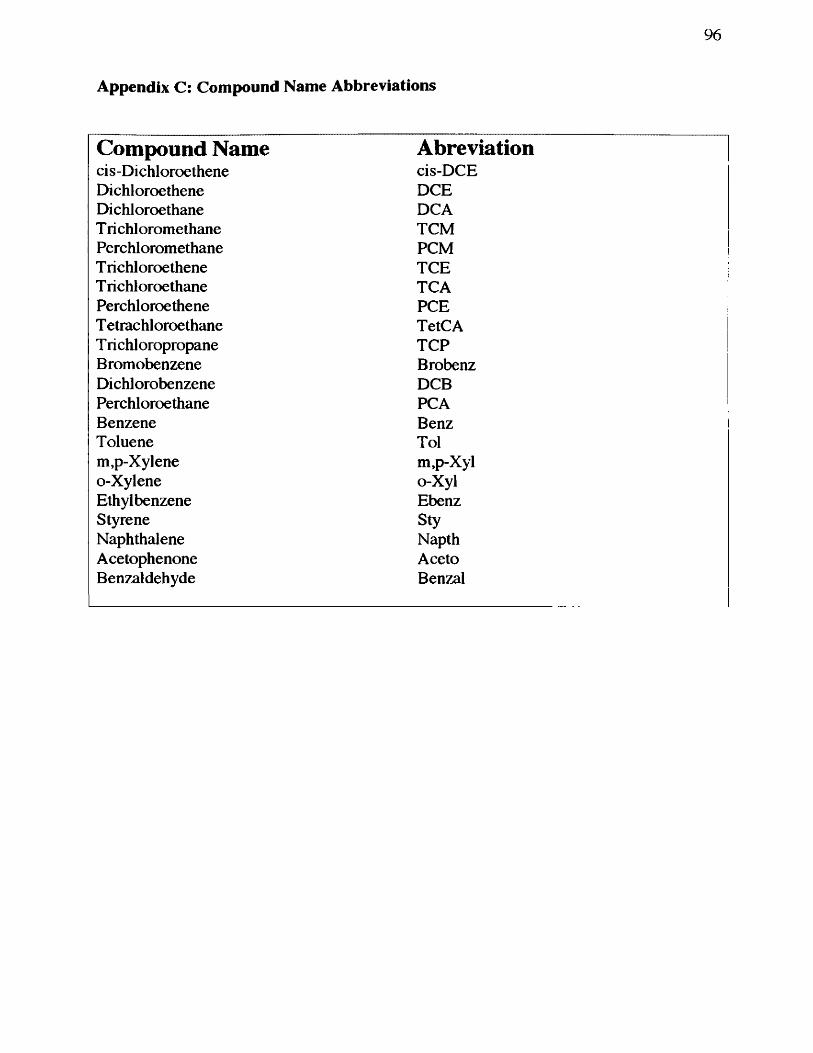
96
Appendix C: Compound Name Abbreviations
Compound Name Abréviationcis-Dichloroethene cis-DCEDichloroethene DCEDichloroethane DCAT richloromethane TCMPerchloromethane PCMTrichloroethene TCET richloroethane TCAPerchloroethene PCET etrachloroethane TetCAT richloropropane TCPBromobenzene BrobenzDichlorobenzene DCBPerchloroethane PCABenzene BenzToluene Toim,p-Xylene m,p-Xylo-Xylene o-XylEthylbenzene EbenzStyrene StyNaphthalene NapthAcetophenone AcetoBenzaldehyde Benzal
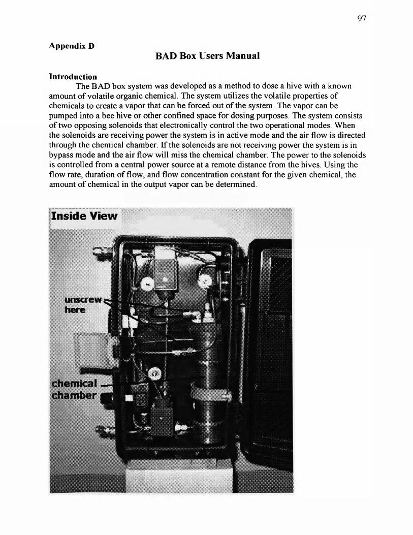
97
Appendix DBAD Box Users Manual
IntroductionThe BAD box system was developed as a method to dose a hive with a known
amount of volatile organic chemical. The system utilizes the volatile properties of chemicals to create a vapor that can be forced out of the system. The vapor can be pumped into a bee hive or other confined space for dosing purposes. The system consists of two opposing solenoids that electronically control the two operational modes. When the solenoids are receiving power the system is in active mode and the air flow is directed through the chemical chamber. If the solenoids are not receiving power the system is in bypass mode and the air flow will miss the chemical chamber. The power to the solenoids is controlled from a central power source at a remote distance from the hives. Using the flow rate, duration of flow, and flow concentration constant for the given chemical, the amount of chemical in the output vapor can be determined.
Inside View
unscrewhere
cm w m r
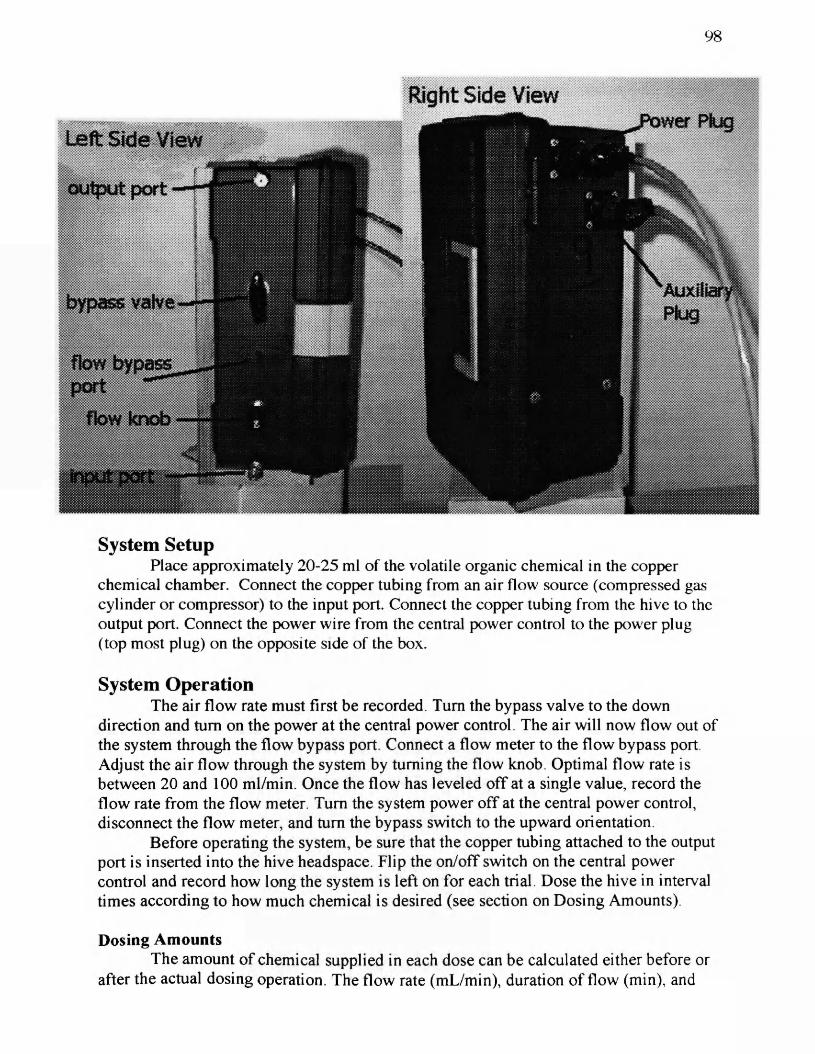
98
Sight Side View
leftside Viemfpm
X v*%
1»
System SetupPlace approximately 20-25 ml of the volatile organic chemical in the copper
chemical chamber. Connect the copper tubing from an air flow source (compressed gas cylinder or compressor) to the input port. Connect the copper tubing from the hive to the output port. Connect the power wire from the central power control to the power plug (top most plug) on the opposite side of the box.
System OperationThe air flow rate must first be recorded. Turn the bypass valve to the down
direction and turn on the power at the central power control. The air will now flow out of the system through the flow bypass port. Connect a flow meter to the flow bypass port Adjust the air flow through the system by turning the flow knob. Optimal flow rate is between 2 0 and 100 ml/min. Once the flow has leveled off at a single value, record the flow rate from the flow meter. Turn the system power off at the central power control, disconnect the flow meter, and turn the bypass switch to the upward orientation.
Before operating the system, be sure that the copper tubing attached to the output port is inserted into the hive headspace. Flip the on/off switch on the central power control and record how long the system is left on for each trial. Dose the hive in interval times according to how much chemical is desired (see section on Dosing Amounts).
Dosing AmountsThe amount of chemical supplied in each dose can be calculated either before or
after the actual dosing operation. The flow rate (mL/min), duration of flow (min), and
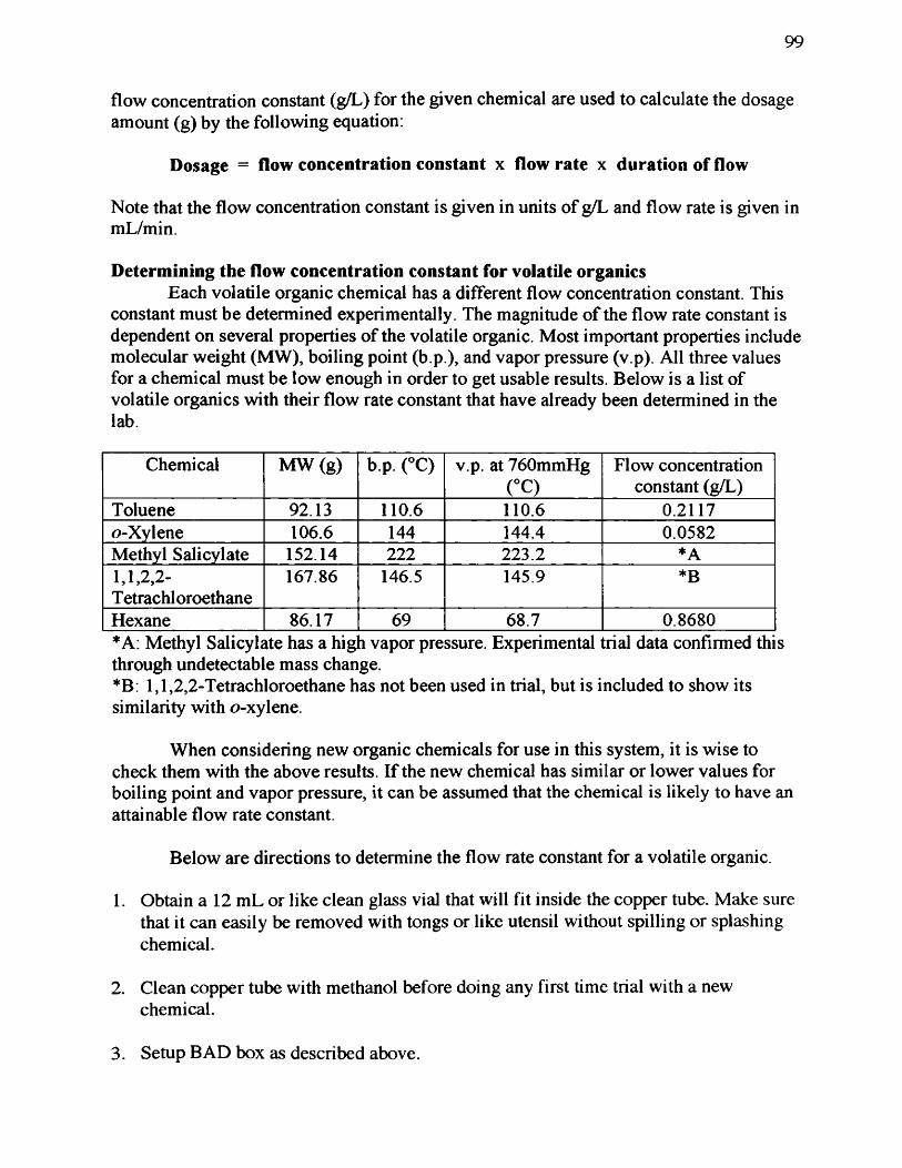
99
flow concentration constant (g/L) for the given chemical are used to calculate the dosage amount (g) by the following equation:
Dosage = flow concentration constant x flow rate x duration of flow
Note that the flow concentration constant is given in units of g/L and flow rate is given in mL/min.
Determining the flow concentration constant for volatile organicsEach volatile organic chemical has a different flow concentration constant. This
constant must be determined experimentally. The magnitude of the flow rate constant is dependent on several properties of the volatile organic. Most important properties include molecular weight (MW), boiling point (b.p ), and vapor pressure (v.p). All three values for a chemical must be low enough in order to get usable results. Below is a list of volatile organics with their flow rate constant that have already been determined in the lab
Chemical MW(g) b.p. ("C> v.p. at 760mmHg CC)
Flow concentration constant (g/L)
Toluene 92.13 1 1 0 . 6 1 1 0 . 6 0.2117o-Xylene 106.6 144 144.4 0.0582Methyl Salicylate 152.14 2 2 2 223.2 *A1 , 1 ,2 ,2 -Tetrachloroethane
167.86 146.5 145.9 *B
Hexane 86.17 69 68.7 0.8680*A: Methyl Salicylate has a high vapor pressure. Experimental trial data confirmed this through undetectable mass change.*B: 1,1,2,2-Tetrachloroethane has not been used in trial, but is included to show its similarity with o-xylene.
When considering new organic chemicals for use in this system, it is wise to check them with the above results. If the new chemical has similar or lower values for boiling point and vapor pressure, it can be assumed that the chemical is likely to have an attainable flow rate constant.
Below are directions to determine the flow rate constant for a volatile organic.
1 . Obtain a 12 mL or like clean glass vial that will fit inside the copper tube. Make sure that it can easily be removed with tongs or like utensil without spilling or splashing chemical.
2. Clean copper tube with methanol before doing any first time trial with a new chemical.
3. Setup BAD box as described above.
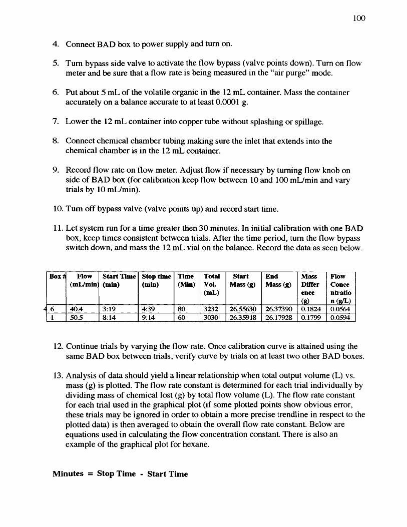
1 0 0
4. Connect BAD box to power supply and turn on.
5. Turn bypass side valve to activate the flow bypass (valve points down). Turn on flow meter and be sure that a flow rate is being measured in the “air purge” mode.
6 . Put about 5 mL of the volatile organic in the 12 mL container. Mass the container accurately on a balance accurate to at least 0 . 0 0 0 1 g.
7. Lower the 12 mL container into copper tube without splashing or spillage.
8 . Connect chemical chamber tubing making sure the inlet that extends into the chemical chamber is in the 12 mL container.
9. Record flow rate on flow meter. Adjust flow if necessary by turning flow knob on side of BAD box (for calibration keep flow between 10 and 100 mL/min and vary trials by 10 mL/min).
10. Turn off bypass valve (valve points up) and record start time.
11. Let system run for a time greater then 30 minutes. In initial calibration with one BAD box, keep times consistent between trials. After the time period, turn the flow bypass switch down, and mass the 12 mL vial on the balance. Record the data as seen below.
Box^ Flow(mlVmin]
Start Time (min)
Stop time (min)
Time(Min)
TotalVol.(mL)
StartMass (g)
EndMass (g)
MassDifference(g)
FlowConcentration (S ^ )
6 n 40.4 3:19 4:39 80 3232 26.55630 26.37390 0.1824 0.05641 50.5 8:14 9:14 60 3030 26.35918 26.17928 0.1799 0.0594
12. Continue trials by varying the flow rate. Once calibration curve is attained using the same BAD box between trials, verify curve by trials on at least two other BAD boxes.
13. Analysis of data should yield a linear relationship when total output volume (L) vs. mass (g) is plotted. The flow rate constant is determined for each trial individually by dividing mass of chemical lost (g) by total flow volume (L). The flow rate constant for each trial used in the graphical plot (if some plotted points show obvious error, these trials may be ignored in order to obtain a more precise trendline in respect to the plotted data) is then averaged to obtain the overall flow rate constant. Below are equations used in calculating the flow concentration constant There is also an example of the graphical plot for hexane.
Minutes = Stop Time - Start Time
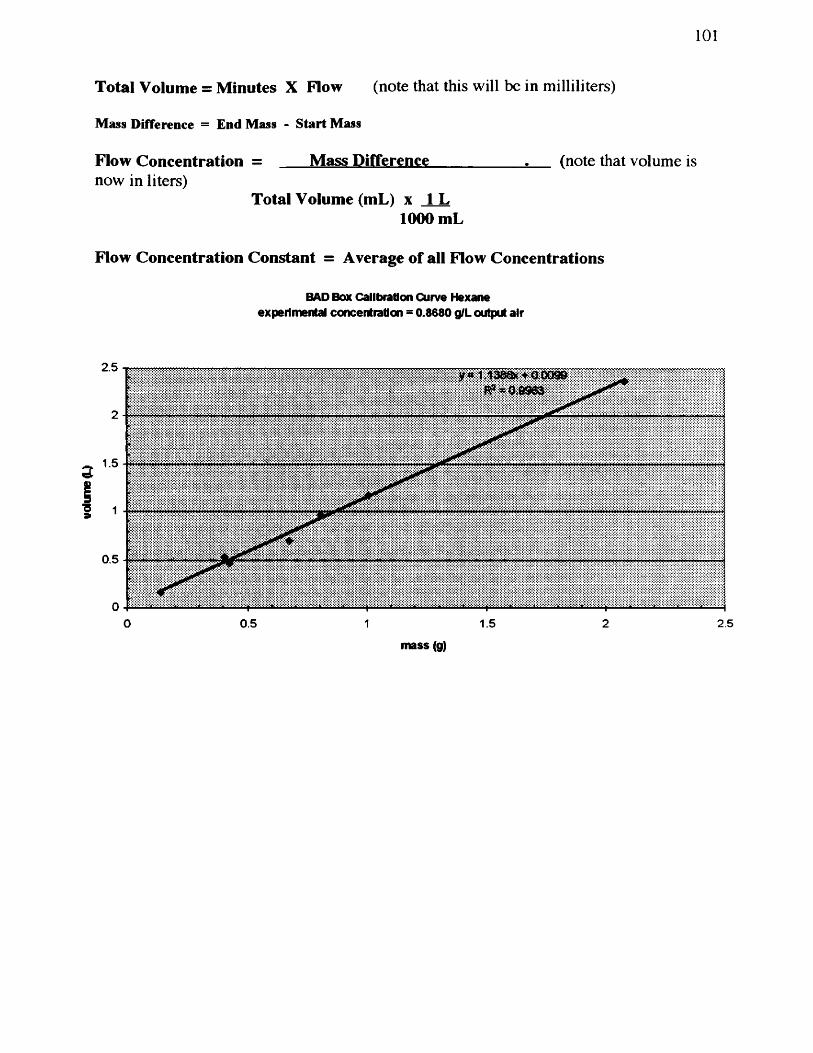
10 1
Total Volume = Minutes X Flow (note that this will be in milliliters)
Mass Difference = End Mass - Start Mass
Flow Concentration = Mass Difference___________. (note that volume isnow in liters)
Total Volume (mL) x 1 L1000 mL
Flow Concentration Constant = Average of all Flow Concentrations
BAD Box Calibration Curve Hexane experimental concentration = 0.8680 gfL output air
2.5
s
?
0.5
0 0.5 1.5 21 2.5
mass (g)
1 0 2
Field Testing of BAD Boxes
Field tests of the BAD boxes were conducted in August 1999. The seven “condo hives” at the BeeAlert! bee yard on the West Campus of the University of Montana were used. The seven hives were outfitted with a BAD boxes on the outside of the condo box with a 1 / 8 inch copper line being run through the condo wall and into the center of the top story of the enclosed hive box. An eighth non condo hive inside the yard was utilized as a reference hive.
A Sears oilless air compressor was used as a pressurized air source. The tank was pressurized to 100 psi. A line was run to a four inch PVC pipe 16 port manifold were the pressure was stepped down to 40 psi using a step down valve attached to the manifold. Copper lines (1/8 inch) were run from the manifold to the BAD box. Flow was set at 50 mL/min on all seven boxes. Five of the seven boxes were loaded with toluene. The boxes were run in the activ mode for ten minutes at the beginning of every hour for ten hours. Concurrent hive VOC samples were taken using the JAG box sampling apparatus and samples were analyzed using TD/GC/MS.
Results Of Field Tests
Two metrics were being utilized for these field tests: Concentration of toluene in the hive and change in flight activity as measured by the flight counters on the condos.
There was no change in flight activity pattern when the toluene vapors were introduced into the hives as compared to flight patterns when just air or no air was being run through the hive.
The toluene concentrations were unmeasurable, not because they were too low, but rather because the levels were so high. The first sample run from a treated hive had so much toluene in it that it flooded the TD/GC/MS system. It took us three weeks to completely clean the system out and be able to run sytem blanks that showed no toluene. Consequently the remaining hive samples were discarded. Three weeks later I ran the non condo hive samples and the concurrent ambient air sample from the yard. These two samples also had so much toluene in them that the system was flooded again and required an extensive flushing and bum off cycle. These two samples may have been contaminated by the hive samples although it is more likely the samples represented true concentrations.
103
Appendix F
A Procedure for the Heat Induced Desorption of VOCs from Hybrid Poplar Leaves
IntroductionHybrid poplar leaves are used for purposes of phytoremediation. They are hearty
trees, grow quickly, have large root balls, extend deep into groundwater, and “pump” a tremendous amount of water from the ground to the atmosphere.
J-Field on Aberdeen Proving Ground is known to be contaminated with several Volatile Organic Compounds (VOCs), Trichloroethene (TCE) and Trichioroethane(TCA) being among them. A grove of hybrid poplar trees were grown over the area where the groundwater was known to be most contaminated. Some VOCs are complexed by the hybrid poplar trees and some are thought to be moved from the groundwater to the atmoshpere being carried along through transpiration. We were interested to know what VOCs were winding up in the leaves of poplars and if they could be enticed to be emmitted from the leaves.
Description of Leaf Desorption ApparatusWe designed a built a special apparatus for this study called the Leaf Desorption
Apparatus (LDA). The body of the LDA is an old GC oven with most of its analytical parts remove, but the heating element and controls still intact and very functional.Copper tubing ( 1 / 8 inch), Swagelok fittings, and Teflon bomb reaction vessels were used to build a carrier gas delivery manifold and a series of chambers inside which the leaves to be desorbed were placed. The carrier gas moves through the manifold, into the teflon vessels where it sweeps the desorbed VOCs in the vessel into an exit tube. The exit tube has a Supelco Carbotrap 400 on its end and the VOCs are trapped on the Carbotrap. All parts except the Carbtraps are inside the oven. Figure 1 is of the LDA.
MethodTwo procedures are involved. First a calibration procedure in order to ascertain
the recoverable amounts of VOCs, then the leaf desorbtion procedure to ascertain the types and amounts of VOCs recoverable from the leaves by this procedure.
Recovery TestFilter paper is spiked with a known amount of VOC. It is then analyzed to
determine the percent VOC recovered. This information is used in studies involving Hybrid poplar tree leaf analysis.Materials:
1 . Nitrile gloves2. Methanol3 . De-ionized water4. 4 140 ml Teflon cylinders5. Syringe
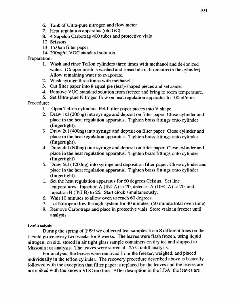
104
6 . Tank of Ultra-pure nitrogen and flow meter7. Heat regulation apparatus (old GC)8 . 4 Supelco Carbotrap 400 tubes and protective vials12. Scissors13. 15.0cm filter paper14. 200ng/ul VOC standard solution
Preparation:1. Wash and rinse Teflon cylinders three times with methanol and de-ionized
water. (Copper mesh is washed and rinsed also. It remains in the cylinder). Allow remaining water to evaporate.
2. Wash syringe three times with methanol.3. Cut filter paper into 8 equal pie (leaf)-shaped pieces and set aside.4. Remove VOC standard solution from freezer and bring to room temperature.5. Set Ultra-pure Nitrogen flow on heat regulation apparatus to lOOml/min.
Procedure:1. Open Teflon cylinders. Fold filter paper pieces into V shape.2. Draw lul (200ng) into syringe and deposit on filter paper. Close cylinder and
place in the heat regulation apparatus. Tighten brass fittings onto cylinder (fingertight).
3. Draw 2ul (400ng) into syringe and deposit on filter paper. Close cylinder and place in the heat regulation apparatus. Tighten brass fittings onto cylinder (fingertight).
4. Draw 4ul (800ng) into syringe and deposit on filter paper. Close cylinder and place in the heat regulation apparatus. Tighten brass fittings onto cylinder (fingertight).
5. Draw 6 ul (1200ng) into syringe and deposit on filter paper. Close cylinder and place in the heat regulation apparatus. Tighten brass fittings onto cylinder (fingertight).
1. Set the heat regulation apparatus for 60 degrees Celsius. Set linetemperatures. Injection A (INJ A) to 70, detector A (DEC A) to 70, and injection B (INJ B) to 25. Start clock simultaneously.
6 . Wait 10 minutes to allow oven to reach 60 degrees.7. Let Nitrogen flow through system for 40 minutes. (50 minute total oven time)8 . Remove Carbotraps and place in protective vials. Store vials in freezer until
analysis.
Leaf AnalysisDuring the spring of 1999 we collected leaf samples from 8 different trees on the
J-Field grove every two weeks for 8 weeks. The leaves were flash frozen, using liquid nitrogen, on site, stored in air tight glass sample containers on dry ice and shipped to Missoula for analysis. The leaves were stored at -25 C untill analysis.
For analysis, the leaves were removed from the freezer, weighed, and placed individually in the teflon cylinder. The recovery procedure described above is basically followed with the exception that filter paper is replaced by the leaves and the leaves are not spiked with the known VOC mixture. After desorption in the LDA, the leaves are
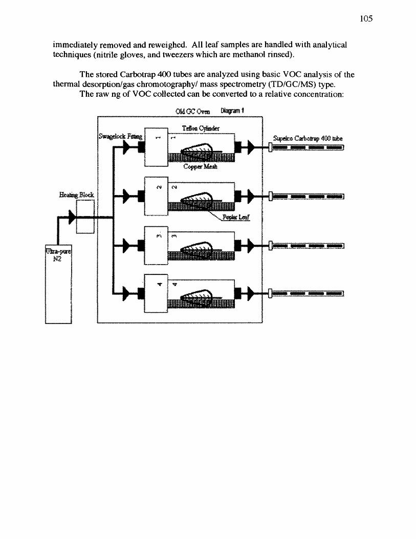
105
immediately removed and reweighed. All leaf samples are handled with analytical techniques (nitrile gloves, and tweezers which are methanol rinsed).
The stored Carbotrap 400 tubes are analyzed using basic VOC analysis of the thermal desorption/gas chromotography/ mass spectrometry (TD/GC/MS) type.
The raw ng of VOC collected can be converted to a relative concentration:
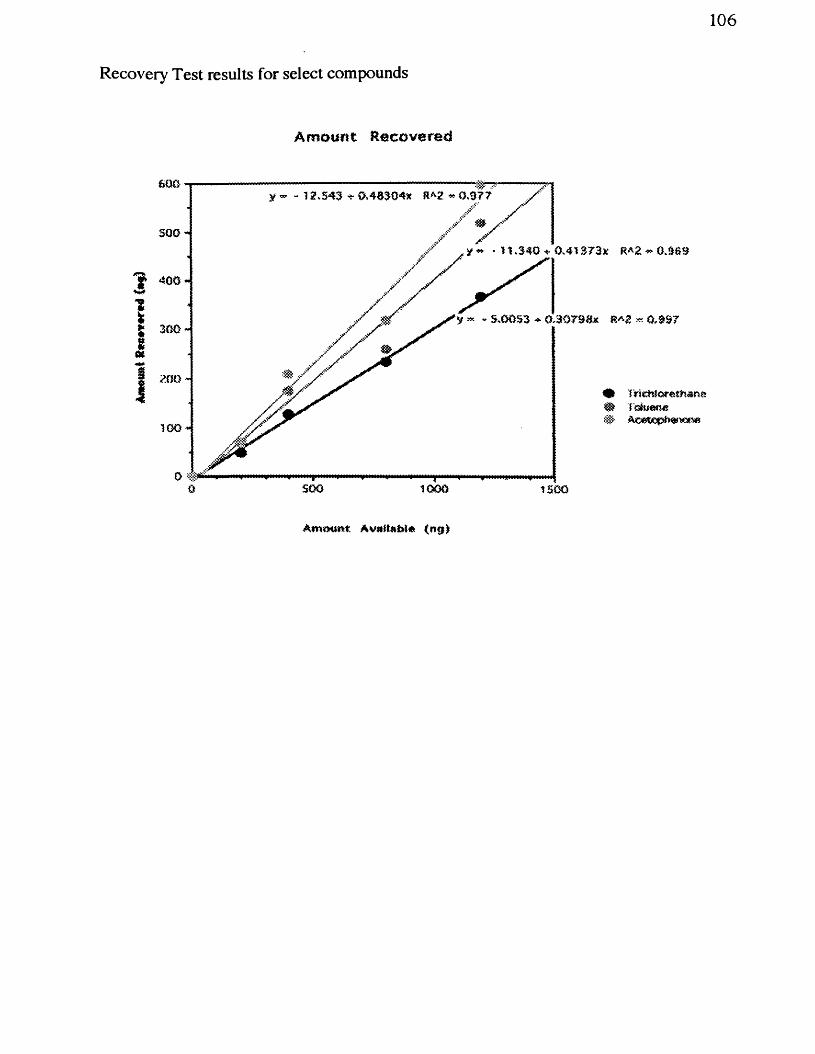
106
Recovery Test results for select compounds
Amount Recovered
y - - 12.543 0.40304% R/ 2 « 0 .977
500y ** - n .340 + 0.41373% R*2 « 0.969
f 400
Î5 300
Iy - 5.0053 4. 0,3079Sx ^ 0,99
I Trj ciîJ orethan e T'ohiene
0 A#o soo
Amount. Avnftoht* (0 3 )
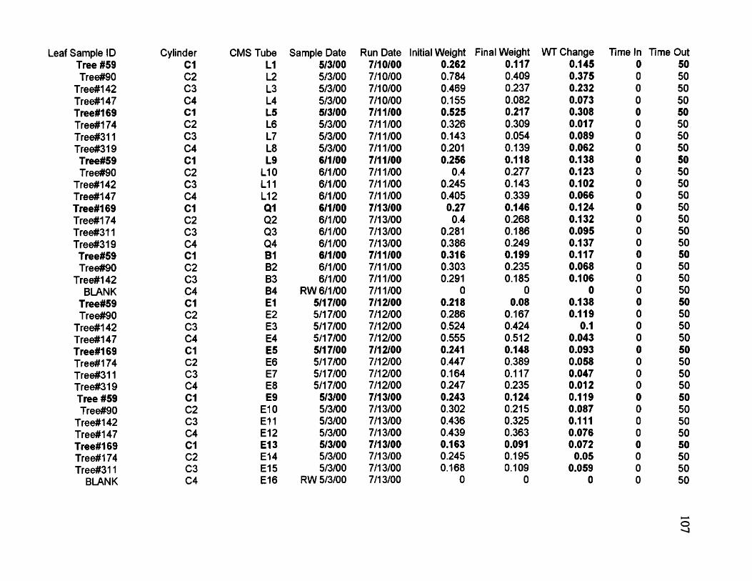
Leaf Sample ID Cylinder OMS Tube Sample Date Run Date Initial Weight Final Weight WT Change Time In Time OutTree #59 01 L I 5/3/00 7/10/00 0.262 0.117 0.145 0 50Tree#90 02 L2 5/3/00 7/10/00 0.784 0.409 0.375 0 50
Tree#142 03 L3 5/3/00 7/10/00 0.469 0.237 0.232 0 50Tree#147 04 L4 5/3/00 7/10/00 0.155 0.082 0.073 0 50Tree#169 01 L5 5/3/00 7/11/00 0.525 0.217 0.308 0 50Tree#174 02 L6 5/3/00 7/11/00 0.326 0.309 0.017 0 50Tree#311 03 L7 5/3/00 7/11/00 0.143 0.054 0.089 0 50Tree#319 04 L8 5/3/00 7/11/00 0.201 0.139 0.062 0 50Tree#59 01 L9 6/1/00 7/11/00 0.256 0.118 0.138 0 50Tree#90 02 L10 6/1/00 7/11/00 0.4 0.277 0.123 0 50
Tree#142 03 L11 6/1/00 7/11/00 0.245 0.143 0.102 0 50Tree#147 04 LI 2 6/1/00 7/11/00 0.405 0.339 0.066 0 50Tree#169 01 01 6/1/00 7/13/00 0.27 0.146 0.124 0 50Tree#174 02 02 6/1/00 7/13/00 0.4 0.268 0.132 0 50Tree#311 03 03 6/1/00 7/13/00 0.281 0.186 0.095 0 50Tree#319 04 04 6/1/00 7/13/00 0.386 0.249 0.137 0 50
Tree#59 01 81 6/1/00 7/11/00 0.316 0.199 0.117 0 50Tree#90 02 B2 6/1/00 7/11/00 0.303 0.235 0.068 0 50
Tree#142 03 B3 6/1/00 7/11/00 0.291 0.185 0.106 0 50BLANK 04 B4 RW 6/1/00 7/11/00 0 0 0 0 50
Tree#59 01 El 5/17/00 7/12/00 0.218 0.08 0.138 0 50Tree#90 02 E2 5/17/00 7/12/00 0.286 0.167 0.119 0 50
Tree#142 03 E3 5/17/00 7/12/00 0.524 0.424 0.1 0 50Tree#147 04 E4 5/17/00 7/12/00 0.555 0.512 0.043 0 50Tree#169 01 E5 5/17/00 7/12/00 0.241 0.148 0.093 0 50Tree#174 02 E6 5/17/00 7/12/00 0.447 0.389 0.058 0 50Tree#311 03 E7 5/17/00 7/12/00 0.164 0.117 0.047 0 50Tree#319 04 E8 5/17/00 7/12/00 0.247 0.235 0.012 0 50Tree #59 01 E9 5/3/00 7/13/00 0.243 0.124 0.119 0 50Tree#90 02 E10 5/3/00 7/13/00 0.302 0.215 0.087 0 50
Tree#142 03 E11 5/3/00 7/13/00 0.436 0.325 0.111 0 50Tree#147 04 E12 5/3/00 7/13/00 0.439 0.363 0.076 0 50Tree#169 01 E13 5/3/00 7/13/00 0.163 0.091 0.072 0 50Tree#174 02 E14 5/3/00 7/13/00 0.245 0.195 0.05 0 50Tree#311 03 E15 5/3/00 7/13/00 0.168 0.109 0.059 0 50
BLANK 04 E16 RW 5/3/00 7/13/00 0 0 0 0 50
o
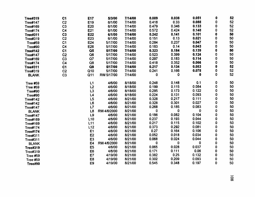
Tree#319 C l E17 5/3/00 7/14/00 0.089 0.038 0.051 0 52Tree#147 02 E19 6/1/00 7/14/00 0.418 0.33 0.088 0 52Tree#169 03 E20 6/1/00 7/14/00 0.479 0.346 0.133 0 52Tree#174 04 E21 6/1/00 7/14/00 0.572 0.424 0.148 0 52Tree#311 03 E22 6/1/00 7/14/00 0.242 0.141 0.101 0 50Tree#319 02 E23 6/1/00 7/14/00 0.151 0.13 0.021 0 50
Tree#59 01 E24 5/17/00 7/14/00 0.284 0.237 0.047 0 50Tree#90 04 E26 5/17/00 7/14/00 0.183 0.14 0.043 0 50
Tree#142 CI 05 5/17/00 7/14/00 0.323 0.184 0.139 0 50Tree#147 02 Q6 5/17/00 7/14/00 0.523 0.399 0.124 0 50Tree#169 03 07 5/17/00 7/14/00 0.297 0.183 0.114 0 50Tree#174 04 08 5/17/00 7/14/00 0.418 0.352 0.066 0 50Tree#311 Cl 09 5/17/00 7/14/00 0.217 0.134 0.083 0 52Tree#319 02 O10 5/17/00 7/14/00 0.241 0.166 0.075 0 52
BLANK 03 011 RW 5/17/00 7/14/00 0 0 0 0 52
Tree #59 L1 4/6/00 8/18/00 0.248 0.148 0.1 0 50Tree #59 L2 4/6/00 8/18/00 0.199 0.115 0.084 0 50Tree#90 L3 4/6/00 8/18/00 0.295 0.173 0.122 0 50Tree#90 L4 4/6/00 8/18/00 0.224 0.131 0.093 0 50
Tree#142 L5 4/6/00 8/21/00 0.328 0.217 0.111 0 50Tree#142 L6 4/6/00 8/21/00 0.328 0.301 0.027 0 50Tree#147 L7 4/6/00 8/21/00 0.268 0.185 0.083 0 50
BLANK L8 RW 4/6/2000 8/21/00 0 0 0 0 50Tree#147 L9 4/6/00 8/21/00 0.186 0.082 0.104 0 50Tree#169 L10 4/6/00 8/21/00 0.237 0.193 0.044 0 50Tree#169 L11 4/6/00 8/21/00 0.217 0.115 0.102 0 50Tree#174 L12 4/6/00 8/21/00 0.373 0.292 0.081 0 50Tree#174 El 4/6/00 8/21/00 0.27 0.164 0.106 0 50Tree#311 E2 4/6/00 8/21/00 0.052 0.018 0.034 0 50Tree#311 E3 4/6/00 8/21/00 0.068 0.024 0.044 0 50
BLANK E4 RW 4/6/2000 8/21/00 0 0 0 0 50Tree#319 E5 4/6/00 8/21/00 0.065 0.028 0.037 0 50Tree#319 E6 4/6/00 8/21/00 0.171 0.111 0.06 0 50Tree #59 E7 4/19/00 8/21/00 0.382 0.25 0.132 0 50Tree #59 E8 4/19/00 8/21/00 0.302 0.209 0.093 0 50Tree#90 E9 4/19/00 8/21/00 0.545 0.348 0.197 0 50
o00
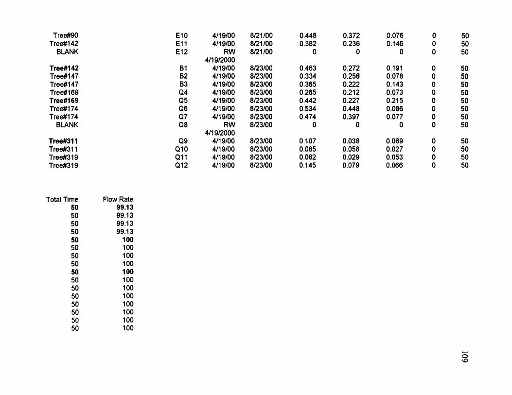
Tree#90 E10 4/19/00 8/21/00 0.448 0.372 0.076 0 50Tree#142 E11 4/19/00 8/21/00 0.382 0.236 0.146 0 50
BLANK E12 RW4/19/2000
8/21/00 0 0 0 0 50
Tree#142 B1 4/19/00 8/23/00 0.463 0.272 0.191 0 50Tree#147 B2 4/19/00 8/23/00 0.334 0.256 0.078 0 50Tree#147 B3 4/19/00 8/23/00 0.365 0.222 0.143 0 50Tree#169 04 4/19/00 8/23/00 0.285 0.212 0.073 0 50Tree#169 05 4/19/00 8/23/00 0.442 0.227 0.215 0 50Tree#174 06 4/19/00 8/23/00 0.534 0.448 0.086 0 50Tree#174 07 4/19/00 8/23/00 0.474 0.397 0.077 0 50
BLANK 08 RW4/19/2000
8/23/00 0 0 0 0 50
Tree#311 09 4/19/00 8/23/00 0.107 0.038 0.069 0 50Tree#311 O10 4/19/00 8/23/00 0.085 0.058 0.027 0 50Tree#319 011 4/19/00 8/23/00 0.082 0.029 0.053 0 50Tree#319 012 4/19/00 8/23/00 0.145 0.079 0.066 0 50
Total Time Flow Rate50 99.1350 99.1350 99.1350 99.1350 10050 10050 10050 10050 10050 10050 10050 10050 10050 10050 10050 100
oVO
en aicncncncnencncncncn0icncncn<ncncncnaic7icncn0icnenui<ncnencnuicncncnci o r o K ) r s 3 0 o o o o o o o N ) r o r o i o o o o o o o o o o o o o o o o o o o o o
oow o o o o o o o o o o o o o o o o o o o o o o o o o o o o o o o o o o oo o o o o o o o o o o o o o o o o o o o o o o o o o o o o o o o o o o
ou
cncncjioicricJiuicncnc/icncncncncntncricncncncnuicncncTtcncncncncntncncncncno o o o o o o o o o o o o o o o o o o o o o o o o o o o o o o o o o o
o o o o o o o o o o o o o o o o o o o o o o o o o o o o o o o o o o op p p p p o p p p o p p p p p p p p p p p p p p p p p p p p o o o o o
III

112
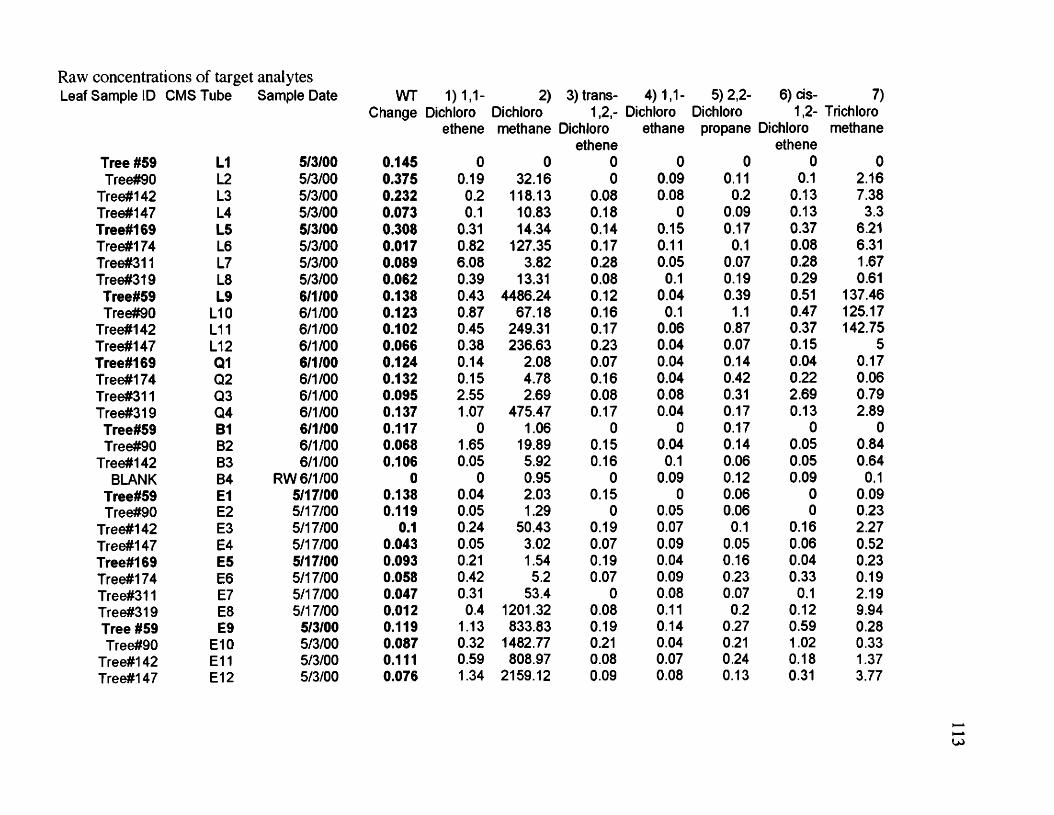
Raw concentrations of target analytesSample ID CMS Tube Sample Date WT 1)1,1- 2) 3) trans- 4)1,1- 5)2.2- 6) cis- 7)
Change Dichloro Dichloro 1,2,- Dichloro Dichloro 1.2- Trichloroethene methane Dichloro
etheneethane propane Dlchloro
ethenemethane
Tree #59 LI 5/3/00 0.145 0 0 0 0 0 0 0Tree#90 L2 5/3/00 0.375 0.19 32.16 0 0.09 0.11 0.1 2.16
Tree#142 L3 5/3/00 0.232 0.2 118.13 0.08 0.08 0.2 0.13 7.38Tree#147 L4 5/3/00 0.073 0.1 10.83 0.18 0 0.09 0.13 3.3Tree#169 L5 5/3/00 0.308 0.31 14.34 0.14 0.15 0.17 0.37 6.21Tree#174 L6 5/3/00 0.017 0.82 127.35 0.17 0.11 0.1 0.08 6.31Tree#311 L7 5/3/00 0.089 6.08 3.82 0.28 0.05 0.07 0.28 1.67Tree#319 L8 5/3/00 0.062 0.39 13.31 0.08 0.1 0.19 0.29 0.61Tree#59 L9 6/1/00 0.138 0.43 4486.24 0.12 0.04 0.39 0.51 137.46Tree#90 L10 6/1/00 0.123 0.87 67.18 0.16 0.1 1.1 0.47 125.17
Tree#142 L11 6/1/00 0.102 0.45 249.31 0.17 0.06 0.87 0.37 142.75Tree#147 L12 6/1/00 0.066 0.38 236.63 0.23 0.04 0.07 0.15 5Tree#169 Q1 6/1/00 0.124 0.14 2.08 0.07 0.04 0.14 0.04 0.17Tree#174 02 6/1/00 0.132 0.15 4.78 0.16 0.04 0.42 0.22 0.06Tree#311 03 6/1/00 0.095 2.55 2.69 0.08 0.08 0.31 2.69 0.79Tree#319 04 6/1/00 0.137 1.07 475.47 0.17 0.04 0.17 0.13 2.89Tree#59 B1 6/1/00 0.117 0 1.06 0 0 0.17 0 0Tree#90 82 6/1/00 0.068 1.65 19.89 0.15 0.04 0.14 0.05 0.84
Tree#142 83 6/1/00 0.106 0.05 5.92 0.16 0.1 0.06 0.05 0.64BLANK 84 RW 6/1/00 0 0 0.95 0 0.09 0.12 0.09 0.1
Tree#59 El 5/17/00 0.138 0.04 2.03 0.15 0 0.06 0 0.09Tree#90 E2 5/17/00 0.119 0.05 1.29 0 0.05 0.06 0 0.23
Tree#142 E3 5/17/00 0.1 0.24 50.43 0.19 0.07 0.1 0.16 2.27Tree#147 E4 5/17/00 0.043 0.05 3.02 0.07 0.09 0.05 0.06 0.52Tree#169 E5 5/17/00 0.093 0.21 1.54 0.19 0.04 0.16 0.04 0.23Tree#174 E6 5/17/00 0.058 0.42 5.2 0.07 0.09 0.23 0.33 0.19Tree#311 E7 5/17/00 0.047 0.31 53.4 0 0.08 0.07 0.1 2.19Tree#319 E8 5/17/00 0.012 0.4 1201.32 0.08 0.11 0.2 0.12 9.94Tree #59 E9 5/3/00 0.119 1.13 833.83 0.19 0.14 0.27 0.59 0.28Tree#90 E10 5/3/00 0.087 0.32 1482.77 0.21 0.04 0.21 1.02 0.33
Tree#142 E11 5/3/00 0.111 0.59 808.97 0.08 0.07 0.24 0.18 1.37Tree#147 E12 5/3/00 0.076 1.34 2159.12 0.09 0.08 0.13 0.31 3.77
w
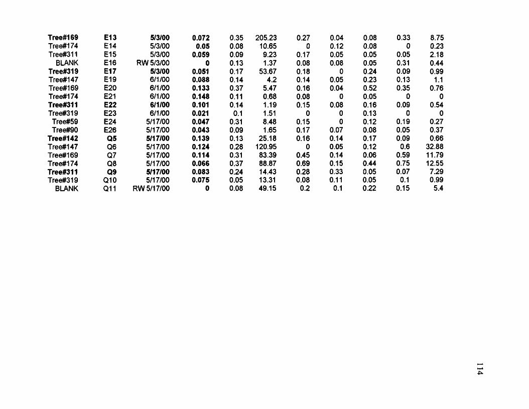
Tree#169 E13 5/3/00 0.072 0.35 205.23 0.27 0.04 0.08 0.33 8.75Tree#174 E14 5/3/00 0.05 0.08 10.65 0 0.12 0.08 0 0.23Tree#311 E15 5/3/00 0.059 0.09 9.23 0.17 0.05 0.05 0.05 2.18
BLANK E16 RW 5/3/00 0 0.13 1.37 0.08 0.08 0.05 0.31 0.44Tree#319 E17 5/3/00 0.051 0.17 53.67 0.18 0 0.24 0.09 0.99Tree#147 E19 6/1/00 0.088 0.14 4.2 0.14 0.05 0.23 0.13 1.1Tree#169 E20 6/1/00 0.133 0.37 5.47 0.16 0.04 0.52 0.35 0.76Tree#174 E21 6/1/00 0.148 0.11 0.68 0.08 0 0.05 0 0Tree#311 E22 6/1/00 0.101 0.14 1.19 0.15 0.08 0.16 0.09 0.54Tree#319 E23 6/1/00 0.021 0.1 1.51 0 0 0.13 0 0Tree#59 E24 5/17/00 0.047 0.31 8.48 0.15 0 0.12 0.19 0.27Tree#90 E26 5/17/00 0.043 0.09 1.65 0.17 0.07 0.08 0.05 0.37
Tree#142 Q5 5/17/00 0.139 0.13 25.18 0.16 0.14 0.17 0.09 0.66Tree#147 Q6 5/17/00 0.124 0.28 120.95 0 0.05 0.12 0.6 32.88Tree#169 Q7 5/17/00 0.114 0.31 83.39 0.45 0.14 0.06 0.59 11.79Tree#174 Q8 5/17/00 0.066 0.37 88.87 0.69 0.15 0.44 0.75 12.55Tree#311 Q9 5/17/00 0.083 0.24 14.43 0.28 0.33 0.05 0.07 7.29Tree#319 Q10 5/17/00 0.075 0.05 13.31 0.08 0.11 0.05 0.1 0.99
BLANK Q11 RW 5/17/00 0 0.08 49.15 0.2 0.1 0.22 0.15 5.4
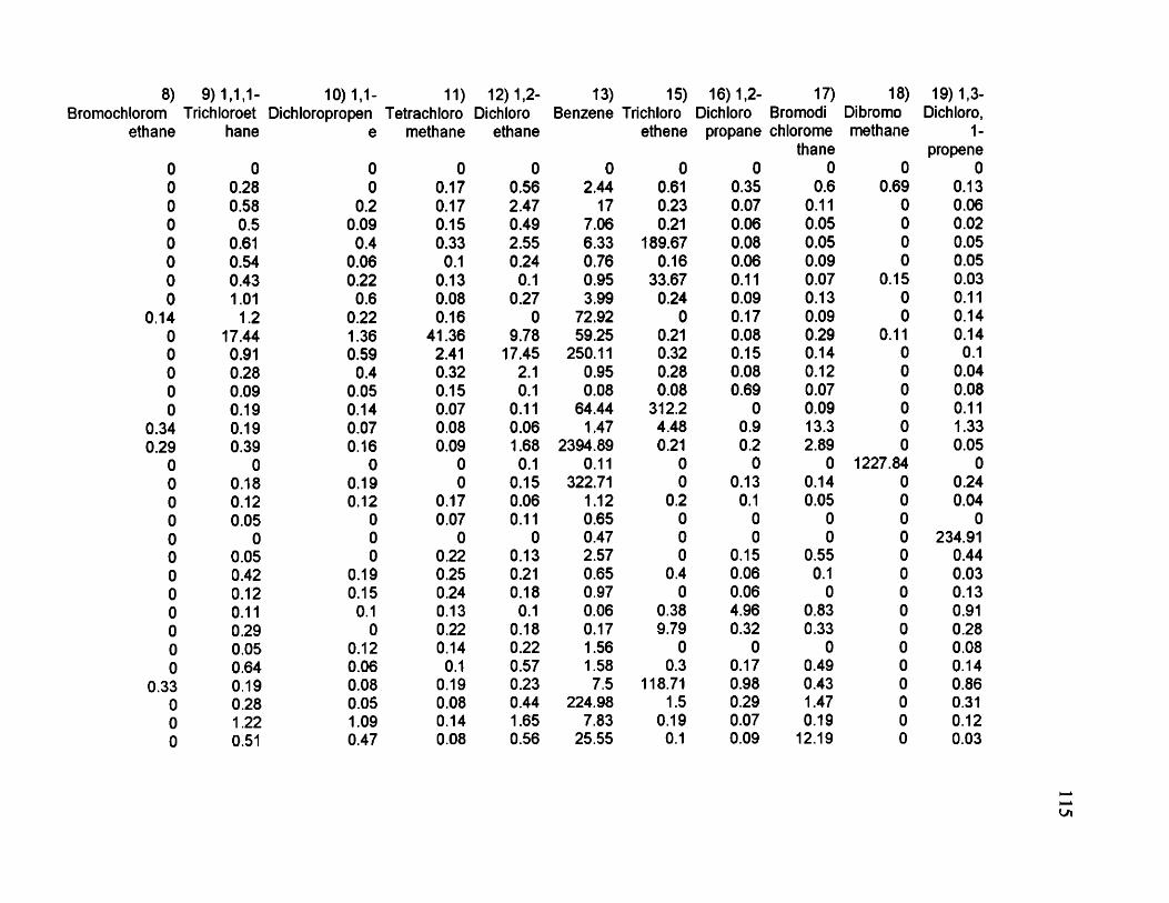
8) 9) 1,1,1- 10)1,1- 11) 12)1.2- 13) 15) 16)1.2- 17) 18) 19)1,3-lorom Trichloroet Dichloropropen Tetrachloro Dichloro Benzene Trichloro Dichloro Bromodl Dibromo Dichloro,ethane hane e methane ethane ethene propane chlorome
thanemethane 1-
propene0 0 0 0 0 0 0 0 0 0 00 0.28 0 0.17 0.56 2.44 0.61 0.35 0.6 0.69 0.130 0.58 0.2 0.17 2.47 17 0.23 0.07 0.11 0 0.060 0.5 0.09 0.15 0.49 7.06 0.21 0.06 0.05 0 0.020 0.61 0.4 0.33 2.55 6.33 189.67 0.08 0.05 0 0.050 0.54 0.06 0.1 0.24 0.76 0.16 0.06 0.09 0 0.050 0.43 0.22 0.13 0.1 0.95 33.67 0.11 0.07 0.15 0.030 1.01 0.6 0.08 0.27 3.99 0.24 0.09 0.13 0 0.11
0.14 1.2 0.22 0.16 0 72.92 0 0.17 0.09 0 0.140 17.44 1.36 41.36 9.78 59.25 0.21 0.08 0.29 0.11 0.140 0.91 0.59 2.41 17.45 250.11 0.32 0.15 0.14 0 0.10 0.28 0.4 0.32 2.1 0.95 0.28 0.08 0.12 0 0.040 0.09 0.05 0.15 0.1 0.08 0.08 0.69 0.07 0 0.080 0.19 0.14 0.07 0.11 64.44 312.2 0 0.09 0 0.11
0.34 0.19 0.07 0.08 0.06 1.47 4.48 0.9 13.3 0 1.330.29 0.39 0.16 0.09 1.68 2394.89 0.21 0.2 2.89 0 0.05
0 0 0 0 0.1 0.11 0 0 0 1227.84 00 0.18 0.19 0 0.15 322.71 0 0.13 0.14 0 0.240 0.12 0.12 0.17 0.06 1.12 0.2 0.1 0.05 0 0.040 0.05 0 0.07 0.11 0.65 0 0 0 0 00 0 0 0 0 0.47 0 0 0 0 234.910 0.05 0 0.22 0.13 2.57 0 0.15 0.55 0 0.440 0.42 0.19 0.25 0.21 0.65 0.4 0.06 0.1 0 0.030 0.12 0.15 0.24 0.18 0.97 0 0.06 0 0 0.130 0.11 0.1 0.13 0.1 0.06 0.38 4.96 0.83 0 0.910 0.29 0 0.22 0.18 0.17 9.79 0.32 0.33 0 0.280 0.05 0.12 0.14 0.22 1.56 0 0 0 0 0.080 0.64 0.06 0.1 0.57 1.58 0.3 0.17 0.49 0 0.14
0.33 0.19 0.08 0.19 0.23 7.5 118.71 0.98 0.43 0 0.860 0.28 0.05 0.08 0.44 224.98 1.5 0.29 1.47 0 0.310 1.22 1.09 0.14 1.65 7.83 0.19 0.07 0.19 0 0.120 0.51 0.47 0.08 0.56 25.55 0.1 0.09 12.19 0 0.03
Ln
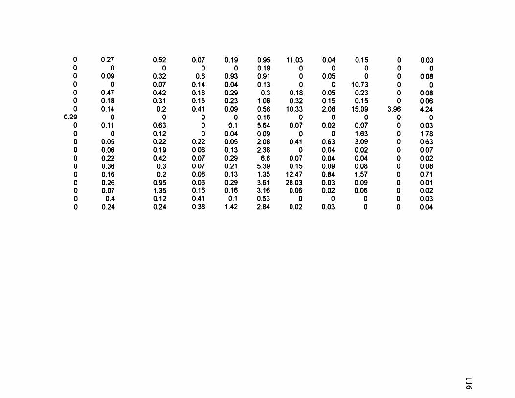
0 0.27 0.52 0.07 0.19 0.95 11.03 0.04 0.15 0 0.030 0 0 0 0 0.19 0 0 0 0 00 0.09 0.32 0.6 0.93 0.91 0 0.05 0 0 0.080 0 0.07 0.14 0.04 0.13 0 0 10.73 0 00 0.47 0.42 0.16 0.29 0.3 0.18 0.05 0.23 0 0.080 0.18 0.31 0.15 0.23 1.06 0.32 0.15 0.15 0 0.060 0.14 0.2 0.41 0.09 0.58 10.33 2.06 15.09 3.96 4.24
0.29 0 0 0 0 0.16 0 0 0 0 00 0.11 0.63 0 0.1 5.64 0.07 0.02 0.07 0 0.030 0 0.12 0 0.04 0.09 0 0 1.63 0 1.780 0.05 0.22 0.22 0.05 2.08 0.41 0.63 3.09 0 0.630 0.06 0.19 0.08 0.13 2.38 0 0.04 0.02 0 0.070 0.22 0.42 0.07 0.29 6.6 0.07 0.04 0.04 0 0.020 0.36 0.3 0.07 0.21 5.39 0.15 0.09 0.08 0 0.080 0.16 0.2 0.08 0.13 1.35 12.47 0.84 1.57 0 0.710 0.26 0.95 0.06 0.29 3.61 28.03 0.03 0.09 0 0.010 0.07 1.35 0.16 0.16 3.16 0.06 0.02 0.06 0 0.020 0.4 0.12 0.41 0.1 0.53 0 0 0 0 0.030 0.24 0.24 0.38 1.42 2.84 0.02 0.03 0 0 0.04
O n
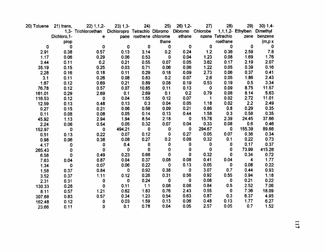
oluene 21) trans, 22)1,1,2- 23)1,3- 24) 25) 26) 1,2- 27) 28) 29) 30) 1,4-1,3- Trichloroethan Dichloropro Tetrachio Dibromo Dibromo Chlorobe 1.1.1.2- Ethylben Dimethyl
Dichloro.l-prop
e pane roethene chlorome thane
ethane nzene Tetrachio roethane
zene benzene(m,px
0 0 0 0 0 0 0 0 0 0 02.91 0.38 0.57 0.13 3.14 0.2 0.24 1.2 0.36 2.59 7.81.17 0.06 0.29 0.06 0.53 0 0.04 1.23 0.08 1.69 1.763.44 0.11 0.2 0.21 0.55 0.07 0.05 3.62 0.17 2.19 2.07
35.19 0.15 0.25 0.03 0.71 0.06 0.06 1.22 0.05 0.39 0.162.28 0.16 0.18 0.11 0.29 0.18 0.09 2.73 0.06 0.37 0.41
3.1 0.11 0.26 0.08 0.83 0.2 0.07 2.6 0.05 1.86 2.431.67 0.12 0.69 0.21 0.89 0.08 0.19 0.53 0.19 0.5 3.34
76.78 0.12 0.57 0.07 10.85 0.11 0.13 0 0.09 8.75 11.57161.01 0.29 2.69 0.1 2.69 0.1 0.2 0.79 0.08 8.14 5.63116.53 0.12 0 0.04 1.55 0.12 0.07 1 0.02 2.72 11.0112.59 0.13 0.48 0.13 0.3 0.04 0.05 1.18 0.02 2.2 2.490.27 0.15 0.21 0.06 0.56 0.09 0.21 0.86 0.8 0.29 0.350.11 0.08 0.08 0.05 0.14 0.13 0.44 1.58 0.3 0.58 0.35
45.92 1.13 2.94 1.94 8.54 2.18 0 15.78 2.39 24.45 37.662.24 0.06 0.54 0.05 0.32 0.07 0.04 0.33 0.08 0.6 0.46
152.97 0 0 494.21 0 0 0 294.67 0 155.39 89.660.51 0.13 0.22 0.07 0.12 0 0.27 0.05 0.07 0.36 0.340.98 0.06 0.36 0.08 0.27 0.2 0.08 0.32 0.1 0.22 0.73417 0 0 0.4 0 0 0 0 0 0.17 0.37
265.43 0 0 0 0 0 0 0 0 73.99 415.266.58 0 0.49 0.23 0.68 0 0 0.32 0 0.34 0.727.63 0.04 0.87 0.04 0.37 0.08 0.08 0.41 0.04 4 1.771.34 0 0.07 0.06 0.22 0 0.13 0.05 0 0.08 0.221.58 0.37 0.84 0 0.92 0.38 0 3.07 0.7 0.44 0.933.52 0.37 1.11 0.12 0.26 0.31 0.56 0.92 0.55 0.94 1.182.31 0.31 0 0 0.24 0 0 0.08 0 0.21 0.22
130.33 0.28 0 0.11 1.1 0.08 0.08 0.84 0.5 2.52 7.068.11 0.57 1.21 0.62 1.83 0.76 2.43 0.55 0 7.36 18.09
307.68 0.83 0.57 0.34 1.23 0.54 0.63 0.87 0.3 6.37 4.95162.48 0.12 0 0.03 1.59 0.13 0.06 0.48 0.13 1.77 6.2723.66 0.11 0 0.1 0.78 0.04 0.05 2.57 0.05 0.7 1.52
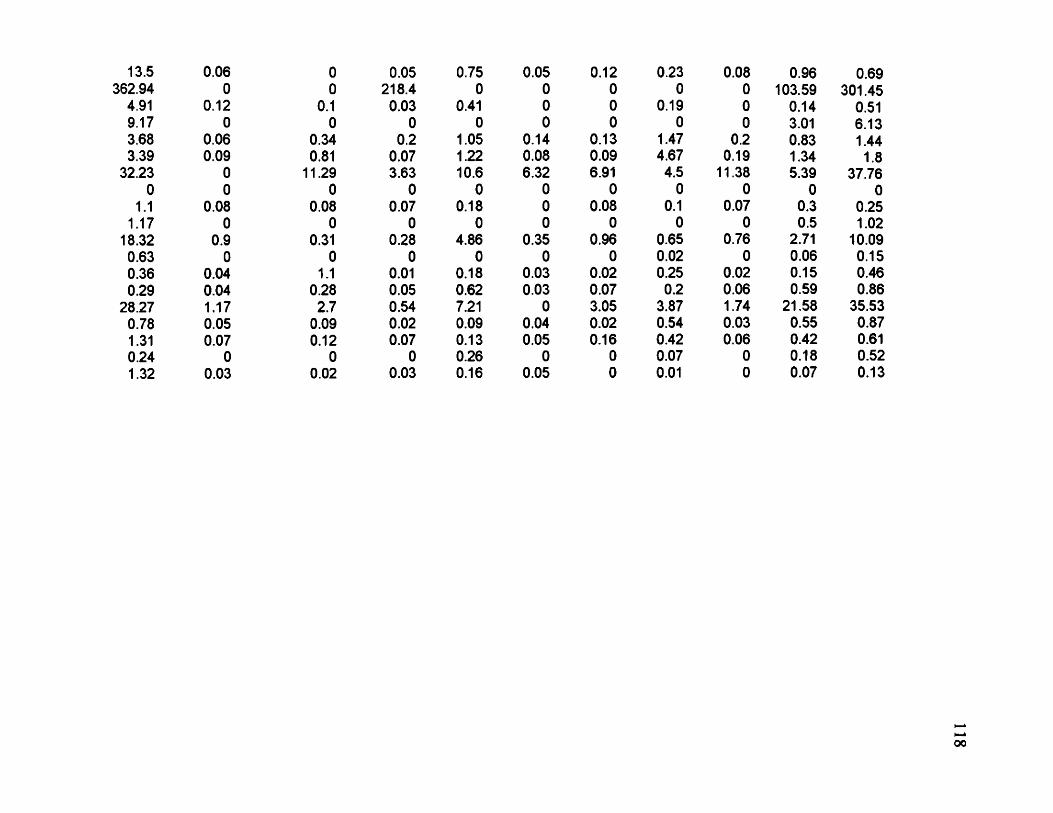
13.5 0.06 0 0.05 0.75 0.05 0.12 0.23 0.08 0.96 0.69362.94 0 0 218.4 0 0 0 0 0 103.59 301.45
4.91 0.12 0.1 0.03 0.41 0 0 0.19 0 0.14 0.519.17 0 0 0 0 0 0 0 0 3.01 6.133.68 0.06 0.34 0.2 1.05 0.14 0.13 1.47 0.2 0.83 1.443.39 0.09 0.81 0.07 1.22 0.08 0.09 4.67 0.19 1.34 1.8
32.23 0 11.29 3.63 10.6 6.32 6.91 4.5 11.38 5.39 37.760 0 0 0 0 0 0 0 0 0 0
1.1 0.08 0.08 0.07 0.18 0 0.08 0.1 0.07 0.3 0251.17 0 0 0 0 0 0 0 0 0.5 1.02
18.32 0.9 0.31 0.28 4.86 0.35 0.96 0.65 0.76 2.71 10.090.63 0 0 0 0 0 0 0.02 0 0.06 0.150.36 0.04 1.1 0.01 0.18 0.03 0.02 0.25 0.02 0.15 0.460.29 0.04 0.28 0.05 0.62 0.03 0.07 0.2 0.06 0.59 0.86
28.27 1.17 2.7 0.54 7.21 0 3.05 3.87 1.74 21.58 35.530.78 0.05 0.09 0.02 0.09 0.04 0.02 0.54 0.03 0.55 0.871.31 007 0.12 0.07 0.13 0.05 0.16 0.42 0.06 0.42 0.610.24 0 0 0 0.26 0 0 0.07 0 0.18 0.521.32 0.03 0.02 0.03 0.16 0.05 0 0.01 0 0.07 0.13
00
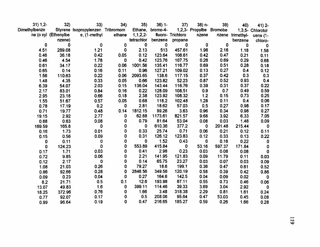
31)1.2- 32) 33) 34) 35) 36)1- 37) 38) n- 39) 40) 41)2-Dimethylbenze Styrene Isopropylenzen Tribromom Ethane, bromo-4- 1,2,3- Propylbe Bromobe 1,3,5- Chlorotol
ne(oxyl (Ethenylbe e, (1-methyl ethane 1,1.2,2- fluoro- Trichloro nzene nzene trimethyl- uene (1-nzene) tetrachior benzene propane benzene chloro-
0 0 0 0 0 0 0 0 0 0 04.51 289.08 1.21 0 2.13 513 457.61 1.96 2.16 1.18 1.580.46 36.18 0.42 0.05 0.12 123.64 108.61 0.42 0.47 0.21 0.110.46 4.54 1.78 0 0.42 123.76 107.75 0.26 0.69 0.29 0.68061 34.17 0.22 0.06 1001.56 135.41 116.77 0.69 0.51 0.28 0.180.65 0.14 0.16 0.11 0.96 127.21 109.02 0.13 027 0.4 0.121.56 110.63 0.22 0.06 2093.65 138.6 117.15 0.37 0.42 0.3 0.31.48 4.35 0.33 0.05 0.66 123.82 52.23 0.87 0.52 0.93 0.46.39 54.07 2.03 0.15 136.04 143.44 116.76 0.39 0.31 0.37 0.222.17 83.01 0.84 0.16 0.22 128.09 108.51 0.9 0.7 0.49 0.592.95 23.18 0.66 0.18 2.38 123.92 108.32 1.2 0.15 0.73 0.251.55 51.67 0.57 005 0.68 118.2 102.48 1.28 0.11 0.4 0.060.78 17.19 0.2 0 2.81 18.62 57.03 0.5 0.27 0.98 0.170.71 19.77 0.48 0.14 1812.15 99.26 3.63 0.96 0.34 0.98 0.27
19.15 2.92 2.77 0 62.88 1173.61 821.57 9.68 3.92 6.33 7.050.88 0.63 0.08 0 0.79 81.64 53.04 0.08 0.03 1.48 0.09
169.59 165.8 0 0 0 610.36 377.2 0 201.48 215.44 00.16 1.73 0.01 0 0.33 25.74 0.71 0.06 0.21 0.12 0.110.15 0.56 0.09 0 0.31 126.12 123.83 0.12 0.33 0.13 0.22
0 0.11 0 0 0 1.52 0.43 0 0.16 0.22 00 124.23 0 0 553.89 415.84 0 53.16 597.37 171.84 0
0.17 1.71 0.03 0 0.41 2.98 0.23 0.03 0.08 0.08 00.72 9.85 0.06 0 2.21 141.95 121.83 0.09 11.79 0.11 0.030.12 2.17 0 0 0.14 65.75 23.27 0.03 0.07 0.03 0.091.08 21.03 0.26 0 79.27 18.6 199.1 0.36 0.47 0.61 0.520.86 92.66 0.28 0 2848.56 349.56 120.19 0.58 0.39 0.42 0.860.09 0.23 0.04 0 0.27 164.6 142.5 0.04 0.09 0.02 0
8.2 21.71 0.5 0.1 12.6 193.98 87.11 0.55 0.73 0.46 0.0613.07 49.83 1.6 0 399.11 114.46 39.33 3.69 3.04 2.92 018.25 372.96 0.76 0 1.66 3.48 318.38 2.29 0.81 1.61 0.240.77 92.07 0.17 0 0.5 208.06 95.64 0.47 53.03 0.45 0.080.99 96.64 0.19 0 0.47 216.65 185.27 0.59 0.26 1.66 0.28
VO
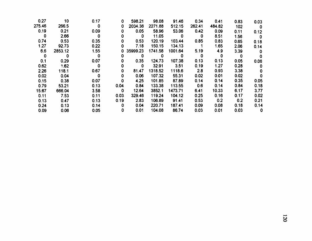
0.27 10 0.17 0 598.21 98.08 91.46 0.34 0.41 0.83 0.03275.46 266.5 0 0 2034.36 2271.88 512.15 262.41 484.82 102 0
0.19 0.21 0.09 0 0.05 58.96 53.06 0.42 0.09 0.11 0.120 2.66 0 0 0 11.05 0 0 8.51 1.56 0
0.74 0.53 0.35 0 0.53 120.19 103.44 0.85 0.83 0.65 0.181.27 92.73 0.22 0 7.18 150.15 134.13 1 1.65 2.06 0.146.6 2853.12 1.55 0 35999.23 1741.58 1001.64 5.19 4.9 3.39 0
0 0 0 0 0 0 0 0 0 0 00.1 0.29 0.07 0 0.35 124.73 107.38 0.13 0.13 0.05 0.06
0.62 1.62 0 0 0 32.91 3.51 0.19 1.27 0.28 02.26 118.1 0.67 0 81.47 1318.52 1118.6 2.8 0.93 3.38 00.02 0.04 0 0 0.06 107.32 55.31 0.02 0.01 0.02 00.15 0.38 0.07 0 4.25 101.85 87.89 0.14 0.14 0.35 0.050.79 53.21 0.13 0.04 0.84 133.38 113.55 0.6 0.14 0.84 0.18
15.67 666.04 3.58 0 12.64 3852.1 1473.71 6.41 10.33 6.17 3.770.11 7.53 0.11 003 329.46 119.24 104.12 0.25 0.16 0.17 0.020.13 0.47 0.13 0.19 2.83 106.89 91.41 0.53 0.2 0.2 0.210.24 0.13 0.14 0 0.04 220.71 187.41 0.09 0.08 0.18 0.140.09 0.06 0.05 0 0.01 104.08 86.74 0.03 0.01 0.03 0
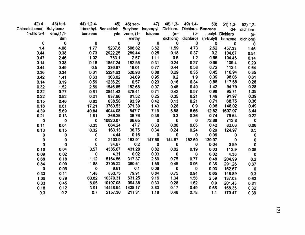
42)4- 43) terl- 44) 1,2,4- 45) 46) sec- 47) 48)1,3- 49) 1,4- 50) 51)1,2- 52) 1,2-otoluene( Butylbenz trimethyl- Benzaldeh Butylben Isopropyl Dlchloro- Dichloro- Benzene d4- dlchloro-1-chloral ene,(1,1- benzene yde zene, (1- toluene (m- (p- , butyl- Dichloro (o-
dim methy dichloro) dichloro) (n-Butyl) benzene dichloro)0 0 0 0 0 0 0 0 0 0 0
1.4 4.08 1.77 5237.8 508.82 3.62 1.59 4.73 2.62 457.33 1.450.44 0.38 0.73 2922.25 289.44 0.25 0.18 0.37 0.2 104.67 0.540.47 2.46 1.02 783.1 2.57 1.11 0.6 1.2 0.66 104.45 0.140.14 0.38 0.18 1857.24 182.55 0.31 0.24 0.27 0.66 109.4 0.290.44 0.49 0.5 336.67 18.01 0.77 0.44 0.53 0.72 112.4 0.640.36 0.34 0.61 5324.63 520.93 0.88 0.29 0.35 0.45 116.94 0.350.42 1.41 0.63 363.02 34.69 0.95 0.2 1.9 0.39 98.06 0.610.14 0.19 0.59 1236.29 0.57 0.23 0.16 0.34 0.88 117.58 0.280.32 1.52 2.59 1546.85 152.68 0.97 0.45 0.49 1.42 94.79 0.280.32 0.77 0.61 3841.43 378.41 0.71 0.42 0.57 0.98 95.71 1.350.22 0.52 0.31 837.66 81.52 0.25 0.35 0.21 1.49 91.97 0.390.15 0.46 0.83 638.58 93.39 0.42 0.13 0.21 0.71 68.75 0.360.18 0.61 17.21 3760.53 371.39 1.43 0.28 0.9 0.98 148.02 0.494.39 5.69 40.84 4044.08 547.7 7.19 5.88 8.66 12.82 1607.97 3.440.21 0.13 1.81 366.25 36.76 0.38 0.3 0.36 0.74 79.64 0.22
0 0 0 10820.07 66.65 0 0 0 72.86 712.8 00.11 0.04 0.33 664.24 47.7 0.33 0.06 0.05 042 82.03 0.060.13 0.15 0.32 163.13 36.75 0.34 0.24 0.24 0.29 124.97 0.5
0 0 0 4.44 0.16 0 0 0 0.06 0 00 0 0 2103.9 163.91 147.69 144.67 152.69 139.97 0 00 0 0 34.67 0.2 0 0 0 0.04 0.59 0
0.18 0.04 0.57 4385.67 431.28 0.82 0.02 0.19 0.03 112.9 0.050.09 002 0 4.31 0.02 0.03 0 0 0.02 4.38 00.68 0.18 1.12 5164.56 317.37 2.59 0.75 0.77 0.48 204.99 0.20.84 0.09 1.88 3705.22 360.51 1.59 0.45 0.96 0.36 291.26 0.67
0 0.05 0 9.61 0.1 0.08 0 0 0.03 152.67 00.33 0.11 1.48 833.75 79.91 0.84 0.75 0.94 0.65 148.89 0.31.06 0.79 60.82 10370.31 631.25 9.16 1.34 1.58 2.39 137.03 0.630.33 0.45 6.05 10107.08 994.38 0.33 0.28 1.62 0.9 201.43 0.810.18 0.12 3.91 14448.94 1438.17 3.83 0.17 0.49 0.65 158.35 0.32
0.3 0.2 0.7 2157.36 211.31 1.18 0.48 0.78 1.1 170.47 0.39
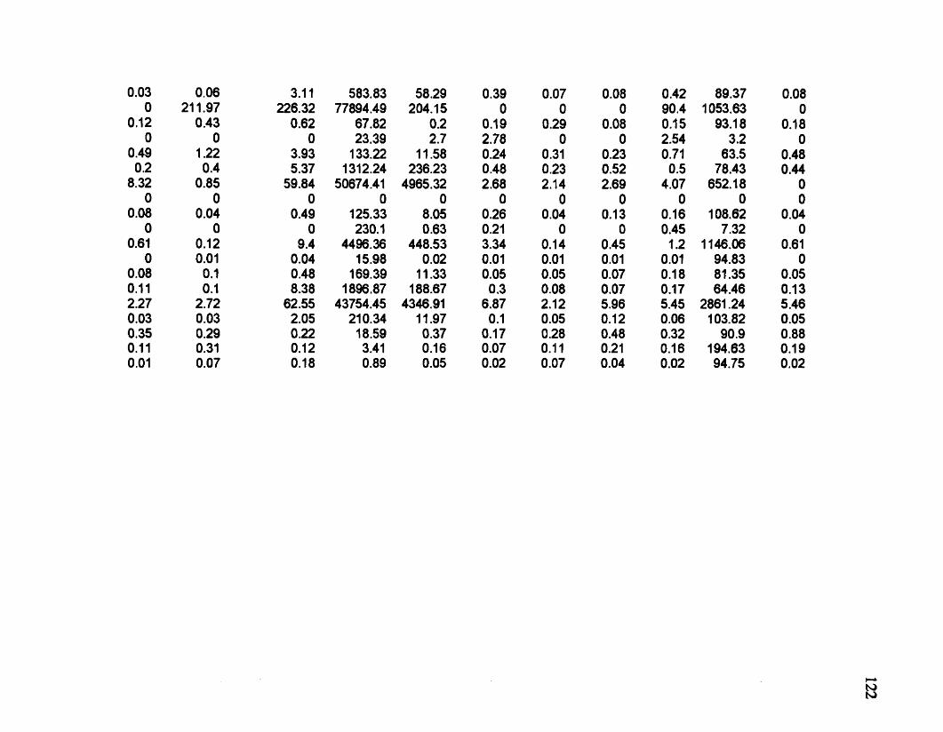
0.03 0.06 3.11 583.83 58.29 0.39 0.07 0.08 0.42 89.37 0.080 211.97 226.32 77894.49 204.15 0 0 0 90.4 1053.63 0
0.12 0.43 0.62 67.82 0.2 0.19 0.29 0.08 0.15 93.18 0.180 0 0 23.39 2.7 2.78 0 0 2.54 3.2 0
0.49 1.22 3.93 133.22 11.58 0.24 0.31 0.23 0.71 63.5 0.480.2 0.4 5.37 1312.24 236.23 0.48 0.23 0.52 0.5 78.43 0.44
8.32 0.85 59.84 50674.41 4965.32 2.68 2.14 2.69 4.07 652.18 00 0 0 0 0 0 0 0 0 0 0
0.08 0.04 0.49 125.33 8.05 0.26 0.04 0.13 0.16 108.62 0.040 0 0 230.1 0.63 0.21 0 0 0.45 7.32 0
0.61 0.12 9.4 4496.36 448.53 3.34 0.14 0.45 1.2 1146.06 0.610 0.01 0.04 15.98 0.02 0.01 0.01 0.01 0.01 94.83 0
0.08 0.1 0.48 169.39 11.33 0.05 0.05 0.07 0.18 81.35 0.050.11 0.1 838 1896.87 188.67 0.3 0.08 0.07 0.17 64.46 0.132.27 2.72 62.55 43754.45 4346.91 6.87 2.12 5.96 5.45 2861.24 5.460.03 0 03 2.05 210.34 11.97 0.1 0.05 0.12 0.06 103.82 0.050.35 0.29 0.22 18.59 0.37 0.17 0.28 0.48 0.32 90.9 0.880.11 0.31 0.12 3.41 0.16 0.07 0.11 0.21 0.16 194.63 0.190.01 0.07 0.18 0.89 0.05 0.02 0.07 0.04 0.02 94.75 0.02
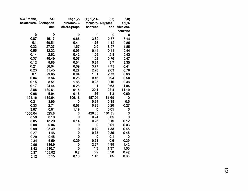
53) Ethane, 54) 55) 1.2- 56) 1,2,4- 57) 58)hexachloro- Acetophen dibromo-3- trichloro- Naphthal 1,2,3-
one chloro-propa benzene ene trichloro-benzene
0 0 0 0 0 00.87 16.17 0.86 3.82 2.77 5.14
0.1 59.51 0.41 1.76 1.12 2.850.33 27.27 1.57 12.9 8.97 4.850.06 32.22 0.05 044 0.41 0.440.14 2.62 0.42 1.05 2.8 0.420.37 40.49 0.07 1.02 0.76 0.470.12 8.86 0.54 6.84 3.7 3.350.21 56.64 0.09 3.77 4.75 0.410.23 31.45 0.27 2.78 2.63 0.78
0.1 99.88 0.04 1.01 2.73 0.660.04 3.64 0.25 0.16 0.94 0.580.15 8.51 1.68 0.23 0.16 0.360.17 24.44 0.28 1 0.63 1.042.88 139.61 61.5 20.1 23.4 11.190.06 5.04 0.15 1.36 1.3 0.69
1121.16 189.64 506.18 487.04 81.69 00.21 3.95 0 0.84 0.38 0.50.33 2.71 0.08 0.25 0.26 0.273.07 0.81 1.19 0 0.05 0
1550.04 525.8 0 420.85 101.35 00.59 0.16 0 0.24 0.05 00.05 48.29 0.14 0.28 0.19 0.120.08 0.04 0 0 0.01 0030.99 28.39 0 0.79 1.38 0.450.27 1.46 0 0.38 0.86 0.450.29 0.45 0 0 0.1 00.34 6.59 0.29 0.91 0.6 0.390.96 136.9 0 2.67 4.98 1.421.43 216.7 0 1.3 1.37 1.060.37 153.82 0.2 0.9 0.58 0.420.12 5.15 0.16 1.18 0.65 0.65
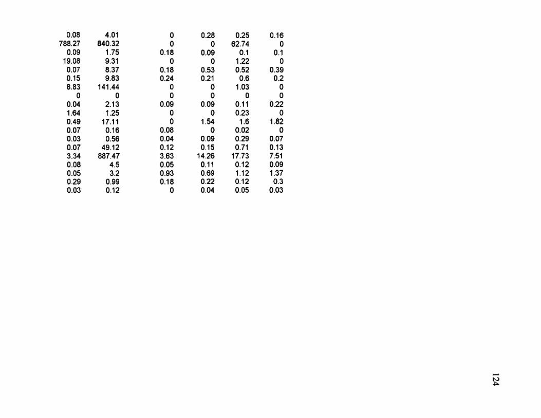
0.08 4.01 0 0.28 0.25 0.16788.27 840.32 0 0 62.74 0
0.09 1.75 0.18 0.09 0.1 0.119.08 9.31 0 0 1.22 00.07 8.37 0.18 0.53 0.52 0.390.15 9.83 0 24 0.21 0.6 0.28.83 141.44 0 0 103 0
0 0 0 0 0 00.04 2.13 0.09 0.09 O il 0.221.64 1.25 0 0 0.23 00.49 17.11 0 154 1.6 1820.07 0.16 0.08 0 0.02 00.03 0.56 0.04 0.09 0.29 0.070.07 49.12 0.12 0.15 0.71 0.133.34 887.47 3.63 14.26 17.73 7.510.08 4.5 0.05 O il 0.12 0.090.05 3.2 0.93 0.69 1.12 1.370.29 0.99 0.18 0.22 0.12 0.30.03 0.12 0 0.04 0.05 0.03


