Using published data in Mendelian randomization: a blueprint for efficient identification of causal risk factors

Using published data in Mendelian randomization:a blueprint for efficient identification of causal risk

factors

Stephen Burgess 1 ∗ Robert A. Scott 2 Nicholas J. Timpson 3

George Davey-Smith 3 Simon G. Thompson 1

EPIC-InterAct Consortium

1 Department of Public Health and Primary Care,University of Cambridge, UK

2 MRC Epidemiology Unit, University of Cambridge, UK3 MRC Integrative Epidemiology Unit, University of Bristol, UK

January 6, 2015

Running head: Published data in Mendelian randomization

Keywords: Mendelian randomization, causal inference, instrumental variable, two-sample, summarized data.

∗Corresponding author: Dr Stephen Burgess. Address: Department of Public Health and PrimaryCare, Strangeways Research Laboratory, 2 Worts Causeway, Cambridge, CB1 8RN, UK. Telephone:+44 1223 748651. Fax: +44 1223 748658. Email: [email protected].

1

Abstract

Finding individual-level data for adequately-powered Mendelian randomization anal-

yses may be problematic. As publicly-available summarized data on genetic associa-

tions with disease outcomes from large consortia are becoming more abundant, use of

published data is an attractive analysis strategy for obtaining precise estimates of the

causal effects of risk factors on outcomes. We detail the necessary steps for conduct-

ing Mendelian randomization investigations using published data, and present novel

statistical methods for combining data on the associations of multiple (correlated or

uncorrelated) genetic variants with the risk factor and outcome into a single causal

effect estimate. A two-sample analysis strategy may be employed, in which evidence

on the gene–risk factor and gene–outcome associations are taken from different data

sources. These approaches allow the efficient identification of risk factors that are

suitable targets for clinical intervention from published data, although the ability to

assess the assumptions necessary for causal inference is diminished.

Methods and guidance are illustrated using the example of the causal effect of

serum calcium levels on fasting glucose concentrations. The estimated causal effect

of a 1 standard deviation (0.13 mmol/L) increase in calcium levels on fasting glucose

(mM) using a single lead variant from the CASR gene region is 0.044 (95% credible

interval -0.002, 0.100). In contrast, using our method to account for the correlation

between variants, the corresponding estimate using 17 genetic variants is 0.022 (95%

credible interval 0.009, 0.035), a more clearly positive causal effect. (232 words)

Key words: Mendelian randomization; instrumental variable; causal inference;

published data; two-sample Mendelian randomization; summarized data.

2

Introduction

Mendelian randomization is a technique which uses genetic variants to assess whethera risk factor, such as a biomarker, has a causal effect on a disease outcome in anon-experimental (observational) setting [1, 2]. We assume that the chosen geneticvariants are associated with the risk factor, but not associated with any confounder ofthe risk factor–outcome relationship, nor associated with the outcome via any pathwayother than that through the risk factor of interest [3]. These three assumptions formthe definition of an instrumental variable [4]. A variant satisfying these assumptionsdivides a study population into subgroups which are analogous to treatment arms ina randomized controlled trial, in that they differ systematically with respect to therisk factor of interest, but not with respect to confounding factors [5]. An associationbetween the genetic variant and the outcome therefore implies that the risk factor hasa causal effect on the outcome.

Mendelian randomization is a valuable approach for identifying risk factors aspotential targets for clinical or behavioural intervention [6]. Evidence from Mendelianrandomization has been used to prioritize investigation of certain biomarkers as causalrisk factors for cardiovascular disease: for example lipoprotein(a) [7], and interleukin-6receptor [8]; and to de-prioritize others: fibrinogen [9], C-reactive protein [10], and uricacid [11]. However, it may be hard to find a suitable study population with sufficientdata on the genetic variants, and both the risk factor and outcome of interest. Asmany genetic variants only explain a small proportion of the variation in the riskfactor, large sample sizes (in some cases comprising tens of thousands of individuals[12]) may be required for adequately-powered Mendelian randomization investigations.Several consortia with large numbers of participants, such as CARDIoGRAMplusC4Dfor coronary artery disease [13] and DIAGRAM for type 2 diabetes [14], have publisheddata on the association of catalogues of genetic variants with either risk factors ordisease status (a list of consortia is given in Web Table A1). These provide preciseestimates of genetic associations which can be used to obtain causal estimates basedon Mendelian randomization in a fast and cost-effective way. In this paper, we providea blueprint for this approach.

Methods

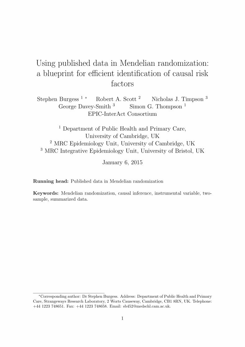
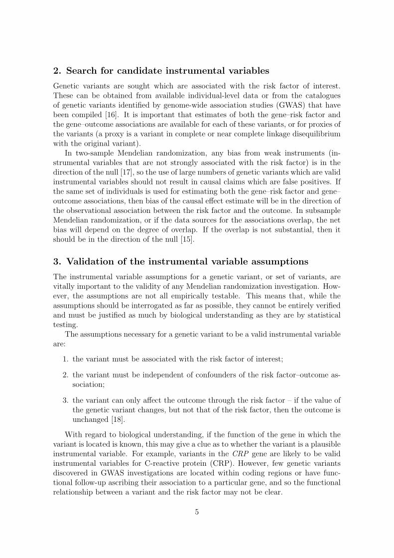
The steps involved in a Mendelian randomization investigation are: 1) specificationof the dataset(s) for analysis, 2) search for candidate instrumental variables, 3) vali-dation of the instrumental variable assumptions, 4) estimation of the causal effect (ifappropriate), 5) supplementary and sensitivity analyses. A schematic diagram of therelevant components in a Mendelian randomization analysis is given in Figure 1. Weproceed to outline each of these steps.

3

��

��

��

��

��

��

��

Figure 1: Schematic diagram outlining the Mendelian randomization approach.

1. Specification of the dataset(s) for analysis

Traditionally, Mendelian randomization analyses have been performed on a singlestudy or studies containing data on genetic variants, and both the risk factor and out-come of interest. The main advantages of using published data rather than individual-level data are their size and scope. The associations of these variants with the riskfactor and outcome in large consortia are likely to be more precisely estimated than ina single study. However, it is unlikely that published data on the genetic associationswith the risk factor, with the outcome, and with potential confounders are availableon the same set of studies.

Two-sample Mendelian randomization is a strategy in which evidence on the as-sociations of genetic variants with the risk factor and with the outcome comes fromnon-overlapping data sources [15]. The limiting factor for the power of a Mendelianrandomization analysis using a given set of genetic variants is the precision in theestimate of the genetic association with the outcome, as this association is typicallymuch weaker than the genetic association with the risk factor. Published data on ge-netic associations with the outcome can therefore be combined with individual-leveldata from a cross-sectional study on genetic variants and the risk factor to obtainprecise Mendelian randomization estimates. If the study used to estimate geneticassociations with the risk factor is included in the estimate of the genetic associationwith the outcome, then this is a subsample rather than a two-sample analysis strat-egy. Alternatively, published data can be used in all aspects of the analysis. In thiscase, the two published data sources may overlap (for example, they both constitutemeta-analyses and some studies are included in both sources).

In any case, it is likely that the sets of individuals used in the gene–risk factor andgene–outcome arms of the analysis will not be identical. An important assumptionto ensure the validity of the analysis is that the two sets represent samples takenfrom the same underlying population. If this is not the case, then inferences maybe misleading, as the association of the genetic variants with the risk factor may notbe replicated in the set of individuals in which the association with the outcome isestimated, or a variant may not be a valid instrumental variable in both sets.

4

2. Search for candidate instrumental variables

Genetic variants are sought which are associated with the risk factor of interest.These can be obtained from available individual-level data or from the cataloguesof genetic variants identified by genome-wide association studies (GWAS) that havebeen compiled [16]. It is important that estimates of both the gene–risk factor andthe gene–outcome associations are available for each of these variants, or for proxies ofthe variants (a proxy is a variant in complete or near complete linkage disequilibriumwith the original variant).

In two-sample Mendelian randomization, any bias from weak instruments (in-strumental variables that are not strongly associated with the risk factor) is in thedirection of the null [17], so the use of large numbers of genetic variants which are validinstrumental variables should not result in causal claims which are false positives. Ifthe same set of individuals is used for estimating both the gene–risk factor and gene–outcome associations, then bias of the causal effect estimate will be in the direction ofthe observational association between the risk factor and the outcome. In subsampleMendelian randomization, or if the data sources for the associations overlap, the netbias will depend on the degree of overlap. If the overlap is not substantial, then itshould be in the direction of the null [15].

3. Validation of the instrumental variable assumptions

The instrumental variable assumptions for a genetic variant, or set of variants, arevitally important to the validity of any Mendelian randomization investigation. How-ever, the assumptions are not all empirically testable. This means that, while theassumptions should be interrogated as far as possible, they cannot be entirely verifiedand must be justified as much by biological understanding as they are by statisticaltesting.

The assumptions necessary for a genetic variant to be a valid instrumental variableare:

1. the variant must be associated with the risk factor of interest;

2. the variant must be independent of confounders of the risk factor–outcome as-sociation;

3. the variant can only affect the outcome through the risk factor – if the value ofthe genetic variant changes, but not that of the risk factor, then the outcome isunchanged [18].

With regard to biological understanding, if the function of the gene in which thevariant is located is known, this may give a clue as to whether the variant is a plausibleinstrumental variable. For example, variants in the CRP gene are likely to be validinstrumental variables for C-reactive protein (CRP). However, few genetic variantsdiscovered in GWAS investigations are located within coding regions or have func-tional follow-up ascribing their association to a particular gene, and so the functionalrelationship between a variant and the risk factor may not be clear.

5

With regard to statistical testing, the simplest and perhaps most effective way ofassessing the instrumental variable assumptions is to test the association of the candi-date genetic variants with a range of covariates which are potential confounders usingindividual-level data. While there is no way of testing the association of the variantswith unknown or unmeasured confounders, for several diseases many of the covariateshaving the strongest association with the outcome (and therefore the greatest poten-tial to bias causal effect estimates) are known and often measured in epidemiologicalstudies. Associations with several covariates can also be assessed from the literature,for example by searching for associations of the variants in a GWAS catalogue [16].However, a key advantage of individual-level data over published data for validationis the ability to test the associations of the candidate instrumental variables with arange of covariates in a systematic way.

One difficulty with this assessment of the instrumental variable assumptions is theproblem of multiple testing. If there are many covariates and multiple genetic vari-ants, then a hypothesis testing approach that accounts for the multiple comparisonsmay lead to a lack of power to detect any specific association. Additionally, as severalcovariates (or the genetic variants) may be correlated, a simple Bonferroni correctionmay be an over-correction. A second difficulty is that genetic variants can be asso-ciated with a covariate without violating the instrumental variable assumptions. If,for example, a genetic variant which is a candidate instrumental variable for bodymass index (BMI) is also associated with blood pressure levels, this may be due tothe causal effect of BMI on blood pressure and not due to a pleiotropic effect of thevariant (pleiotropy means that a variant has multiple effects). If the genetic associa-tion with a covariate is entirely mediated through the risk factor of interest, then theinstrumental variable assumptions are not violated. In this case, taking the exampleabove, the coefficient in the regression of blood pressure on the genetic variant shouldbe substantially attenuated on adjustment for BMI. However, attenuation may notbe complete, due to possible measurement error in the intermediate variable (here,BMI), and as the genetic variant is not independent of blood pressure conditional onBMI due to the presence of confounding factors between BMI and blood pressure [3].

A practical way to proceed is to specify two sets of genetic variants to be usedas instrumental variables: a ‘conservative’ set, for which the minimum p-value forthe association of each variant with a covariate is greater than a pre-specified level(say p > 0.01), and a ‘liberal’ set, for which the minimum p-value for each variantis greater than the Bonferroni corrected p-value (p > 0.05

Vwhere V is the number of

covariates tested). If this approach is followed, to minimize the possibility of biasdue to pleiotropy, the Mendelian randomization estimate using the ‘conservative’ setof variants should be regarded as the primary analysis and the estimate using the‘liberal’ set as the secondary analysis.

Other violations of the instrumental variable assumptions, such as populationstratification, are more difficult to test using only summarized data. This particularissue is discussed in the Web Appendix in the context of the applied example.

6

4. Estimation of the causal effect

We assume that estimates and standard errors (or equivalently estimates and p-values)are available for the genetic associations with the risk factor and with the outcome.Initially we assume that the scenario is two-sample Mendelian randomization andall the genetic variants considered are uncorrelated (in linkage equilibrium). Theseassumptions are later relaxed.

Genetic variants uncorrelated (linkage equilibrium)

For each of K genetic variants (k = 1, . . . , K), we represent the estimate of the geneticassociation with the risk factor as Xk with standard error σXk, and the estimate of thegenetic association with the outcome as Yk with standard error σY k. Usually, thesegenetic associations are per allele effects: the change in the risk factor or outcome foreach additional copy of the minor (or effect) allele. If the outcome is binary, then Yk

is usually the regression coefficient from a logistic regression, representing a log oddsratio.

Two methods have been proposed for the estimation of a causal effect from thesesummarized estimates: an inverse-variance weighted method [19], and a likelihood-based method [20]. When the genetic associations with the risk factor are preciselyestimated, both approaches give similar estimates. When there is considerable im-precision in the estimates, causal effect estimates from the inverse-variance weightedmethod are over-precise, while the likelihood-based method gives appropriately-sizedconfidence intervals.

The causal estimate from the inverse-variance weighted method (βIV W ) is:

βIV W =

∑Kk=1XkYkσ

−2Y k∑K

k=1X2kσ

−2Y k

. (1)

The approximate standard error of the estimate is:

se(βIV W ) =

√1∑K

k=1X2kσ

−2Y k

. (2)

The inverse-variance weighted estimator can be motivated as a weighted averageof the ratio estimates Yk

Xkfor each variant k, weighted using the reciprocal of an

approximate expression for their asymptotic varianceσ2Y k

X2k(inverse-variance weighting,

as in a meta-analysis) [21]. The estimate βIV W expresses the causal increase in theoutcome (or log odds of the outcome for a binary outcome) per unit change in therisk factor. The relationship between the risk factor and the outcome is assumed tobe linear.

The estimate from the likelihood-based method (βL) is obtained from the likelihood

7

function of the model:

Xk ∼ N (ξk, σ2Xk) (3)

Yk ∼ N (βLξk, σ2Y k) for k = 1, . . . , K.

Estimates and confidence intervals can be obtained by direct maximization of thelikelihood, or from Bayesian methods. The likelihood-based method can be motivatedas finding the linear relationship between the coefficients Xk and Yk which best fits thedata, allowing for the uncertainty in both sets of coefficients. As above, the likelihood-based estimator expresses the causal increase in the outcome per unit change in therisk factor assuming a linear association between the risk factor and outcome variables.

These models assume that the data sources for the association estimates withthe risk factor and with the outcome are non-overlapping. If they overlap, then thecoefficients Xk and Yk will be correlated in their distributions. The likelihood-basedmethod can be modified to accommodate this by considering a bivariate model of(Xk, Yk) for each genetic variant (see [20]).

Genetic variants correlated (linkage disequilibrium)

If the genetic variants are correlated, then estimates from the inverse-variance weightedmethod will overstate precision. If estimates are available of the correlations be-tween variants, then the likelihood-based method can be modified by assuming amultivariate normal distribution for the genetic associations with the risk factorX = (Xk; k = 1, . . . K) and with the outcome Y = (Yk; k = 1, . . . K), with esti-mates of these correlations used in the variance–covariance matrices. The correlationbetween the coefficients for the associations of two genetic variants with the risk fac-tor (as well as with the outcome) are equal to the correlation between the variantsthemselves:

X ∼ NK(ξ,ΣX) (4)

Y ∼ NK(βLξ,ΣY )

where the matrix component ΣXij = σXiσXjρij, with σXi being the standard error ofthe coefficient Xi and ρij the correlation between variants i and j (and ρii = 1 forall i). Likewise ΣY ij = σY iσY jρij. Software code for implementing these methods isprovided in the Web Appendix.

Again, if the data sources for the association estimates are overlapping then a jointnormal model for the genetic associations (X,Y) can be estimated:(

XY

)∼ N2K

((ξ

βLξ

),

(ΣX ΣXY

ΣY X ΣY

))(5)

where the matrix component ΣXY ij = θσXiσY jρij, with θ representing the correlationbetween the genetic associations with the risk factor and outcome, and ΣXY = ΣT

Y X .The value of θ can be estimated by bootstrapping if the individual-level data is avail-able; otherwise, sensitivity analyses can be undertaken across a range of plausible

8

values.

Supplementary and sensitivity analyses

In addition to the primary analysis to estimate the causal effect of the risk factor onthe outcome, a number of additional analyses can be performed, which fall into thecategories of supplementary or sensitivity analyses.

If there are multiple mechanisms by which the risk factor may affect the outcome,and if genetic variants can be categorized as relating to one or other of these mecha-nisms, then separate Mendelian randomization estimates can be obtained using eachcategory of variants. For example, variants may be associated with BMI by variousmechanisms, such as suppressing appetite or increasing metabolic rate. A Mendelianrandomization estimate constructed using variants associated with BMI through ap-petite suppression more closely represents the causal effect of intervening on BMI viaappetite suppression. Differences in the causal estimates using genetic variants associ-ated with different mechanisms may be informative in understanding the aetiology ofthe disease, and may highlight specific mechanisms to prioritize for pharmacologicalintervention.

If there are variants whose status as instrumental variables is uncertain, thensensitivity analyses can be performed using a more conservative and a more liberalset of genetic variants, as described in step 3. Additionally, if there is no pleiotropyand the effects of the risk factor on the outcome associated with changes in the geneticvariants are homogeneous for all variants, the genetic association estimates with therisk factor and with the outcome should follow a linear relationship passing throughthe origin. By plotting the genetic association estimates with the risk factor and withthe outcome, any points which are not compatible with a straight-line through theorigin (allowing for uncertainty in the estimates) can be investigated for potentialpleiotropy of the variants or for heterogeneity of the causal effect (perhaps due todifferent mechanisms of association with the risk factor).

A formal test for heterogeneity is known as an overidentification test [22]. Ex-amples of overidentification tests with individual-level data include the Basmann test[23] and the Sargan test [24]. A similar test can be derived with summarized datafrom the likelihood-based method to test the hypothesis that the causal effect βL isthe same using all variants: if βL were replaced by βLk, are the differences between theβLk compatible with chance?. By the likelihood ratio test, twice the difference in thelog-likelihood function evaluated at the maximum likelihood estimate with βLk = βL

and evaluated at ξk = Xk, βLkξk = Yk (saturated model) should be distributed as achi-squared variable on K − 1 degrees of freedom under the null hypothesis of homo-geneity.

Example: effect of calcium levels on fasting glucose

Calcium is the most abundant mineral in the body, with a wide range of vital functionsin human biology, including bone development and maintenance, muscle contraction,

9

neurotransmitter release, and exocytosis. Indeed, insulin secretion is a calcium depen-dent process [25], and total serum calcium levels have been associated with glucoseintolerance [26]. Calcium absorption is enhanced by vitamin D, and vitamin D is aputative causal risk factor for type 2 diabetes [27]. We perform a Mendelian ran-domization analysis to investigate the causal effect of serum calcium levels on fastingglucose concentrations to illustrate some of the points discussed above.

For the gene–risk factor associations, we use individual-level baseline data on 6351subcohort participants of European ancestry from the EPIC-InterAct study, a multi-centre case-cohort study of type 2 diabetes nested within the European ProspectiveInvestigation into Cancer and Nutrition (EPIC) [28]. All participants gave writteninformed consent, and the study was approved by the local ethics committees in theparticipating countries and the Internal Review Board of the International Agency forResearch on Cancer. For the gene–outcome associations, we use published data fromthe Meta-Analyses of Glucose and Insulin-related traits Consortium (MAGIC), down-loaded from www.magicinvestigators.org [29]. Data on per allele genetic associationswith fasting glucose are available for up to 133 010 participants without diabetes ofEuropean ancestry from 66 studies. EPIC-InterAct participants were not included inthe MAGIC dataset, so this is a two-sample Mendelian randomization design. Ge-netic variants for both samples were available for variants on the Cardio-Metabochip(Illumina).

Identification of candidate variants and assessment of instru-mental variable assumptions

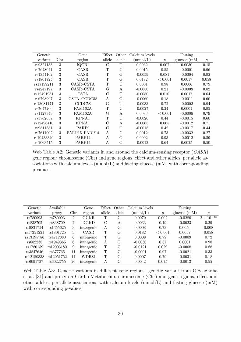
We compare two strategies for choosing genetic variants to include in the Mendelianrandomization analysis. The first strategy is to include only variants from in andaround the calcium-sensing receptor (CASR) gene region [30]. This region was shownto have the strongest association with calcium levels in a GWAS [31] and has knownbiological relevance for calcium metabolism pathways. There are 17 variants withina 500kb range of the CASR gene in various degrees of linkage disequilibrium; thelead variant was rs1801725. The second strategy is to include 10 variants from thedifferent gene regions identified as associated with calcium levels by O’Seaghdha etal. [31]. Suitable proxies were found for the variants which are not available on theCardio-Metabochip. Further details of the data and genetic variants used in theanalysis are given in Web Tables A2 and A3.

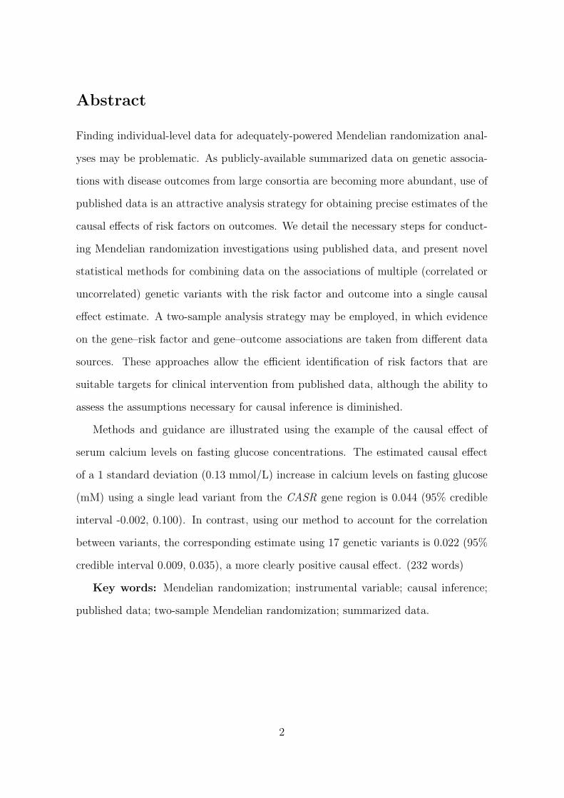
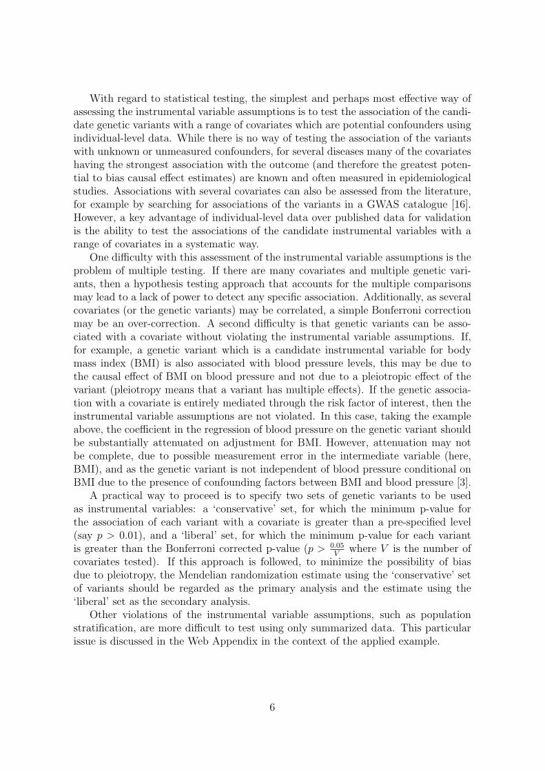
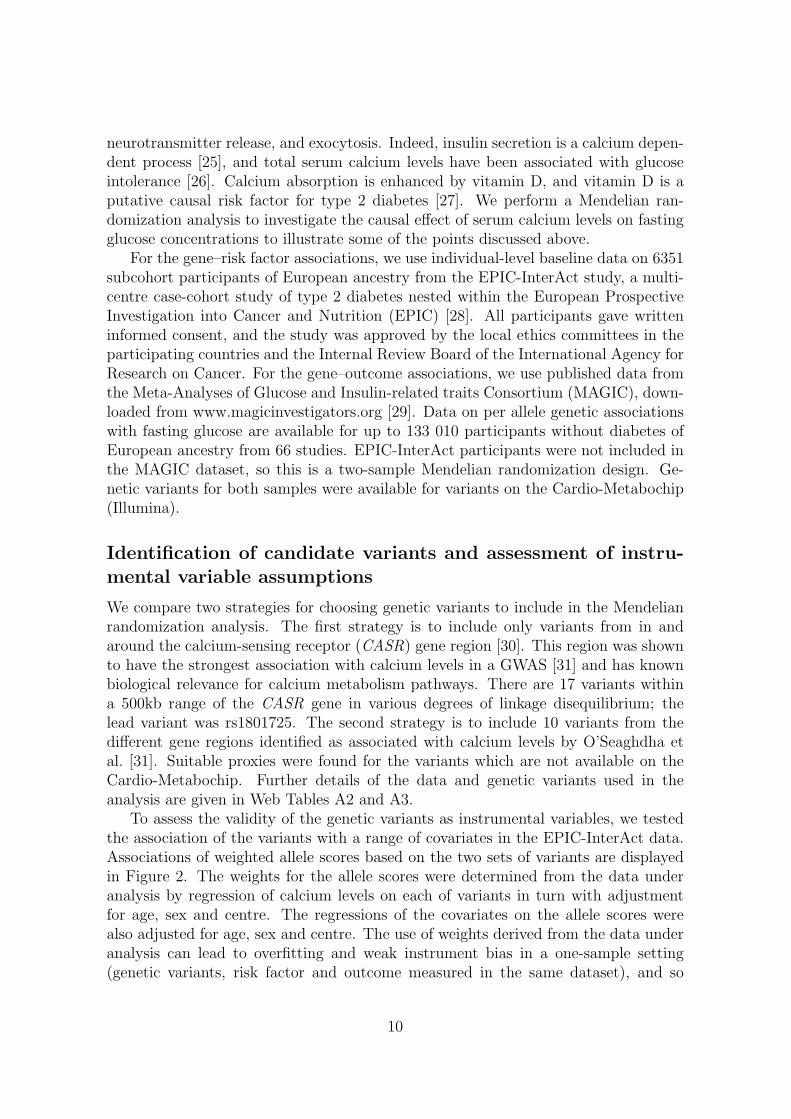
To assess the validity of the genetic variants as instrumental variables, we testedthe association of the variants with a range of covariates in the EPIC-InterAct data.Associations of weighted allele scores based on the two sets of variants are displayedin Figure 2. The weights for the allele scores were determined from the data underanalysis by regression of calcium levels on each of variants in turn with adjustmentfor age, sex and centre. The regressions of the covariates on the allele scores werealso adjusted for age, sex and centre. The use of weights derived from the data underanalysis can lead to overfitting and weak instrument bias in a one-sample setting(genetic variants, risk factor and outcome measured in the same dataset), and so

10

is not recommended for the primary Mendelian randomization analysis where it isimportant to mitigate against false positive results [32].

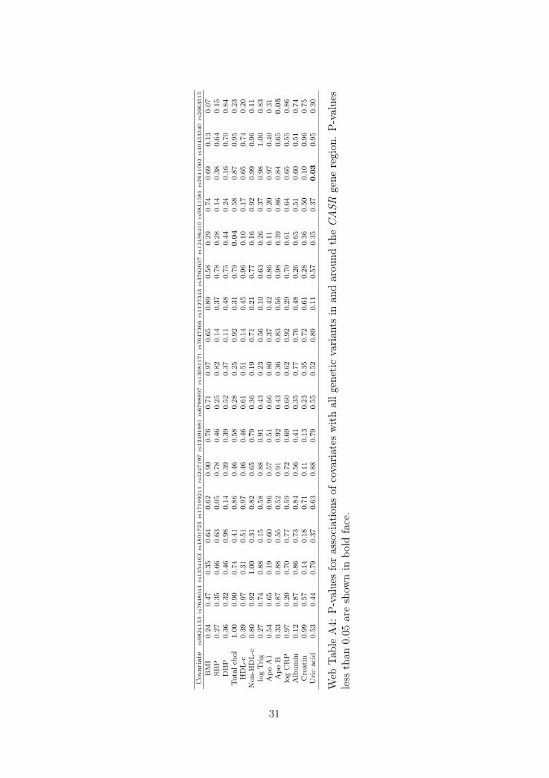
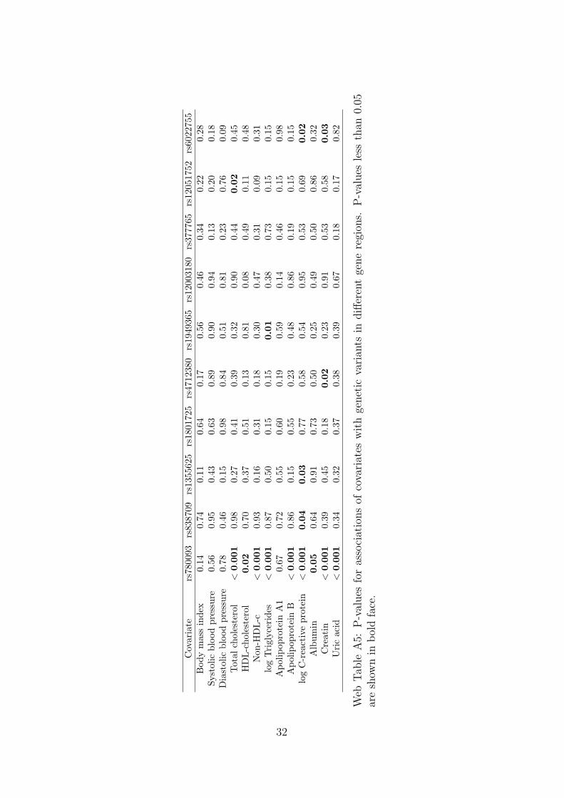
The coefficients represent the standard deviation difference in the covariate asso-ciated with a unit increase in the allele score (which is scaled to be associated with a1 standard deviation [0.13 mmol/L] increase in calcium levels). The allele score basedon variants from the CASR gene region does not show stronger associations with thecovariates than would be expected by chance. A search of the literature revealed asuggestive association between cardiac troponin-T (a regulatory protein integral tomuscle contraction) and a variant near to the CASR locus [33]. However, this asso-ciation may be solely due to the genetic effect on calcium levels, in which case theMendelian randomization assumptions are not violated. No other associations werereported. In contrast, the allele score based on variants from different gene regions isassociated at p < 0.01 with total cholesterol, non–high-density lipoprotein-cholesterol,triglycerides, apolipoprotein B, creatinine, and uric acid, and additionally at p < 0.05with C-reactive protein. Since summarizing a set of genetic variants as an allele scoremay hide pleiotropic effects of particular variants, associations of each of the variantsindividually with the covariates are given in Web Tables A4 and A5; this yields simi-lar conclusions. A discussion on potential population stratification for variants in theCASR gene region is given in the Web Appendix.

Estimation of a causal effect

We proceed to consider causal estimation only using the genetic variants in and aroundthe CASR gene region. The restriction to a single genetic region means that thecausal estimate is likely to apply only to a single mechanism by which calcium levelsaffect fasting glucose, and therefore may not be generalizable to other mechanisms.However, as the genetic region has a plausible mechanistic association with calciumlevels, it is more likely to be a valid causal estimate than one based on variants frommany genetic regions with unknown functional relevance to calcium levels and clearevidence of pleiotropy.

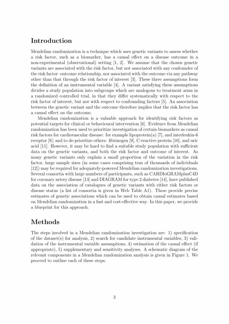
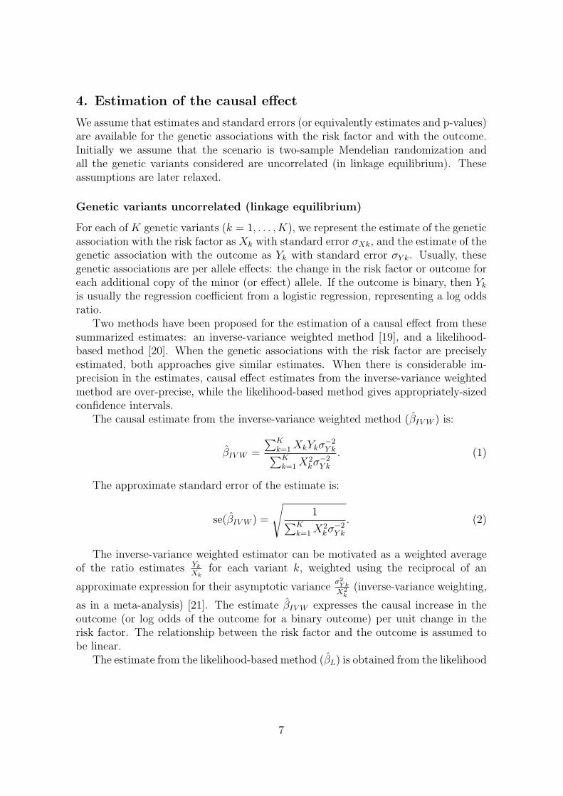
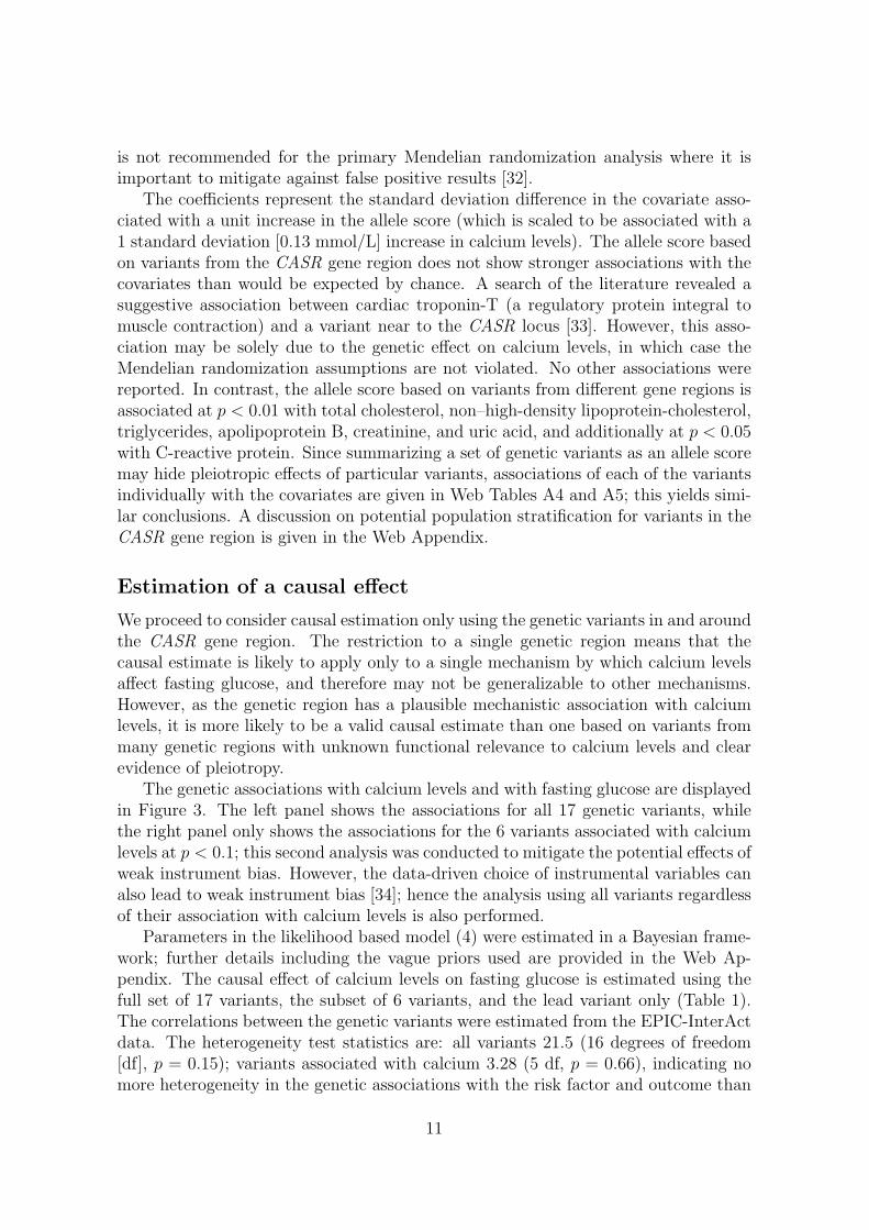
The genetic associations with calcium levels and with fasting glucose are displayedin Figure 3. The left panel shows the associations for all 17 genetic variants, whilethe right panel only shows the associations for the 6 variants associated with calciumlevels at p < 0.1; this second analysis was conducted to mitigate the potential effects ofweak instrument bias. However, the data-driven choice of instrumental variables canalso lead to weak instrument bias [34]; hence the analysis using all variants regardlessof their association with calcium levels is also performed.

Parameters in the likelihood based model (4) were estimated in a Bayesian frame-work; further details including the vague priors used are provided in the Web Ap-pendix. The causal effect of calcium levels on fasting glucose is estimated using thefull set of 17 variants, the subset of 6 variants, and the lead variant only (Table 1).The correlations between the genetic variants were estimated from the EPIC-InterActdata. The heterogeneity test statistics are: all variants 21.5 (16 degrees of freedom[df], p = 0.15); variants associated with calcium 3.28 (5 df, p = 0.66), indicating nomore heterogeneity in the genetic associations with the risk factor and outcome than

11

−0.5 0.0 0.5 1.0

1.00 ( 0.69 , 1.31 )

0.03 ( −0.24 , 0.31 )

0.09 ( −0.23 , 0.40 )

−0.06 ( −0.40 , 0.27 )

0.20 ( −0.09 , 0.50 )

−0.04 ( −0.32 , 0.25 )

0.21 ( −0.08 , 0.50 )

0.20 ( −0.08 , 0.48 )

−0.03 ( −0.32 , 0.25 )

0.09 ( −0.20 , 0.38 )

−0.07 ( −0.37 , 0.23 )

0.16 ( −0.14 , 0.46 )

−0.19 ( −0.45 , 0.07 )

0.17 ( −0.09 , 0.43 )

Covariates

Calcium

Body mass index

Systolic blood pressure

Diastolic blood pressure

Total cholesterol

HDL−cholesterol

Non−HDL−c

log Triglycerides

Apolipoprotein A1

Apolipoprotein B

log C−reactive protein

Albumin

Creatinine

Uric acid

Genetic score using all variants in CASR region

−1.0 0.0 0.5 1.0

1.00 ( 0.73 , 1.27 )

0.08 ( −0.16 , 0.32 )

0.08 ( −0.20 , 0.36 )

0.12 ( −0.18 , 0.41 )

0.34 ( 0.09 , 0.60 )

−0.16 ( −0.40 , 0.09 )

0.39 ( 0.13 , 0.64 )

0.61 ( 0.36 , 0.86 )

0.02 ( −0.23 , 0.27 )

0.34 ( 0.08 , 0.60 )

0.27 ( 0.00 , 0.53 )

0.22 ( −0.04 , 0.48 )

−0.35 ( −0.58 , −0.12 )

0.32 ( 0.10 , 0.55 )

Covariates

Calcium

Body mass index

Systolic blood pressure

Diastolic blood pressure

Total cholesterol

HDL−cholesterol

Non−HDL−c

log Triglycerides

Apolipoprotein A1

Apolipoprotein B

log C−reactive protein

Albumin

Creatinine

Uric acid

Genetic score using variants in different regions

Figure 2: Associations with a range of covariates of weighted allele scores based ongenetic variants associated with calcium levels for: (left) 17 variants in and aroundthe CASR gene region; (right) 10 variants in different gene regions. Estimates arecoefficients for the difference in the covariate measured in standard deviations perunit increase in the allele score (a unit increase in the allele score is scaled to beassociated with a 1 standard deviation [0.13 mmol/L] increase in calcium levels).Coefficients are obtained from the EPIC-InterAct dataset using linear regression withadjustment for age, sex and centre. Lines are 95% confidence intervals.

12

−0.005 0.000 0.005 0.010 0.015 0.020 0.025

−0.

005

0.00

00.

005

0.01

0

Per allele change in calcium levels (mmol/L)

Per

alle

le c

hang

e in

fast

ing

gluc

ose

leve

ls (

mM

)

−0.005 0.000 0.005 0.010 0.015 0.020 0.025

−0.

005

0.00

00.

005

0.01

0

Per allele change in calcium levels (mmol/L)

Per

alle

le c

hang

e in

fast

ing

gluc

ose

leve

ls (

mM

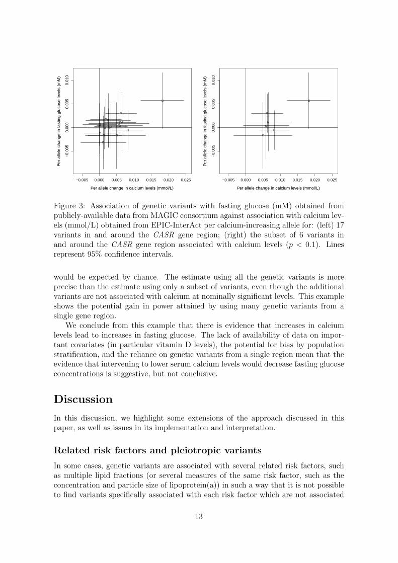
)Figure 3: Association of genetic variants with fasting glucose (mM) obtained frompublicly-available data from MAGIC consortium against association with calcium lev-els (mmol/L) obtained from EPIC-InterAct per calcium-increasing allele for: (left) 17variants in and around the CASR gene region; (right) the subset of 6 variants inand around the CASR gene region associated with calcium levels (p < 0.1). Linesrepresent 95% confidence intervals.

would be expected by chance. The estimate using all the genetic variants is moreprecise than the estimate using only a subset of variants, even though the additionalvariants are not associated with calcium at nominally significant levels. This exampleshows the potential gain in power attained by using many genetic variants from asingle gene region.

We conclude from this example that there is evidence that increases in calciumlevels lead to increases in fasting glucose. The lack of availability of data on impor-tant covariates (in particular vitamin D levels), the potential for bias by populationstratification, and the reliance on genetic variants from a single region mean that theevidence that intervening to lower serum calcium levels would decrease fasting glucoseconcentrations is suggestive, but not conclusive.

Discussion

In this discussion, we highlight some extensions of the approach discussed in thispaper, as well as issues in its implementation and interpretation.

Related risk factors and pleiotropic variants

In some cases, genetic variants are associated with several related risk factors, suchas multiple lipid fractions (or several measures of the same risk factor, such as theconcentration and particle size of lipoprotein(a)) in such a way that it is not possibleto find variants specifically associated with each risk factor which are not associated

13

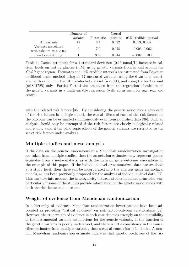
Number of Causalvariants F statistic estimate 95% credible interval

All variants 17 3.4 0.022 0.009, 0.035Variants associated

6 7.9 0.028 -0.003, 0.062with calcium at p < 0.1

Lead variant only 1 30.6 0.044 -0.002, 0.100

Table 1: Causal estimates for a 1 standard deviation (0.13 mmol/L) increase in cal-cium levels on fasting glucose (mM) using genetic variants from in and around theCASR gene region. Estimates and 95% credible intervals are estimated from Bayesianlikelihood-based method using all 17 measured variants, using the 6 variants associ-ated with calcium in the EPIC-InterAct dataset (p < 0.1), and using the lead variant(rs1801725) only. Partial F statistics are taken from the regression of calcium onthe genetic variants in a multivariable regression (with adjustment for age, sex, andcentre).

with the related risk factors [35]. By considering the genetic associations with eachof the risk factors in a single model, the causal effects of each of the risk factors onthe outcome can be estimated simultaneously even from published data [36]. Such ananalysis should only be attempted if the risk factors are closely biologically relatedand is only valid if the pleiotropic effects of the genetic variants are restricted to theset of risk factors under analysis.

Multiple studies and meta-analysis

If the data on the genetic associations in a Mendelian randomization investigationare taken from multiple studies, then the association estimates may represent pooledestimates from a meta-analysis, as with the data on gene–outcome associations inthe example of this paper. If the individual-level or summarized data are availableat a study level, then these can be incorporated into the analysis using hierarchicalmodels, as has been previously proposed for the analysis of individual-level data [37].This can take into account the heterogeneity between studies in a more principled way,particularly if some of the studies provide information on the genetic associations withboth the risk factor and outcome.

Weight of evidence from Mendelian randomization

In a hierarchy of evidence, Mendelian randomization investigations have been ad-vocated as providing “critical evidence” on risk factor–outcome relationships [38].However, the true weight of evidence in each case depends strongly on the plausibilityof the instrumental variable assumptions for the genetic variants. If the function ofthe genetic variants is poorly understood, and there is little consistency in the causaleffect estimates from multiple variants, then a causal conclusion is in doubt. A non-null Mendelian randomization estimate indicates that genetic predictors of the risk

14

factor are also associated with the outcome, but there may be alternative causal path-ways other than that through the risk factor of interest. This is particularly likely ifa large number of variants are included in the analysis, and/or if the justification forusing the variants in the analysis is solely on the basis of observational associationswith the risk factor. Additionally, conclusions may still be limited by a lack of power,particularly if the genetic variants only explain a small proportion of the variance inthe risk factor.

Conclusion

In conclusion, we have here explained why Mendelian randomization is a useful ap-proach for the assessment of risk factors as potential targets for clinical interven-tion. We have demonstrated how published data enable efficient analysis strategiesfor Mendelian randomization experiments. This is a timely development in view ofthe increasing public availability of genetic association estimates in large datasets.The efficiency of these analyses can be improved by using multiple variants in eachgene region, but correlation between the variants must be accounted for.

Acknowledgements

We thank all EPIC participants and staff for their contribution to the study. We thankstaff from the Technical, Field Epidemiology and Data Functional Group Teams ofthe MRC Epidemiology Unit in Cambridge, UK, for carrying out sample preparation,DNA provision and quality control, genotyping and data-handling work. Fundingfor the biomarker measurements in the random subcohort was provided by grants toEPIC-InterAct from the European Community Framework Programme 6 (IntegratedProject LSHM-CT-2006-037197) and to EPIC-Heart from the Medical Research Coun-cil and British Heart Foundation (Joint Award G0800270). Stephen Burgess is sup-ported by the Wellcome Trust (grant number 100114). Simon G. Thompson is sup-ported by the British Heart Foundation (grant number CH/12/2/29428). No specificfunding was received for the writing of this manuscript. The authors have no conflictsof interest.

Conflict of interest

The authors declare that they have no conflict of interest.

References

[1] Davey Smith G, Ebrahim S. ‘Mendelian randomization’: can genetic epidemiol-ogy contribute to understanding environmental determinants of disease? Inter-national Journal of Epidemiology 2003; 32(1):1–22, doi:10.1093/ije/dyg070.

15

[2] Lawlor D, Harbord R, Sterne J, Timpson N, Davey Smith G. Mendelian random-ization: using genes as instruments for making causal inferences in epidemiology.Statistics in Medicine 2008; 27(8):1133–1163, doi:10.1002/sim.3034.

[3] Didelez V, Sheehan N. Mendelian randomization as an instrumental variableapproach to causal inference. Statistical Methods in Medical Research 2007;16(4):309–330, doi:10.1177/0962280206077743.

[4] Greenland S. An introduction to instrumental variables for epidemiologists. Inter-national Journal of Epidemiology 2000; 29(4):722–729, doi:10.1093/ije/29.4.722.

[5] Davey Smith G, Ebrahim S. Mendelian randomization: prospects, potentials,and limitations. International Journal of Epidemiology 2004; 33(1):30–42, doi:10.1093/ije/dyh132.

[6] Burgess S, Butterworth A, Malarstig A, Thompson S. Use of Mendelian randomi-sation to assess potential benefit of clinical intervention. British Medical Journal2012; 345:e7325, doi:10.1136/bmj.e7325.

[7] Kamstrup P, Tybjaerg-Hansen A, Steffensen R, Nordestgaard B. Genetically el-evated lipoprotein(a) and increased risk of myocardial infarction. Journal of theAmerican Medical Association 2009; 301(22):2331–2339, doi:10.1001/jama.2009.801.

[8] The Interleukin-6 Receptor Mendelian Randomisation Analysis Consortium. Theinterleukin-6 receptor as a target for prevention of coronary heart disease: aMendelian randomisation analysis. Lancet 2012; 379(9822):1214–1224, doi:10.1016/s0140-6736(12)60110-x.

[9] Keavney B, Danesh J, Parish S, Palmer A, Clark S, Youngman L, Delepine M,Lathrop M, Peto R, Collins R, et al.. Fibrinogen and coronary heart disease: testof causality by ‘Mendelian randomization’. International Journal of Epidemiology2006; 35(4):935–943, doi:10.1093/ije/dyl114.

[10] CRP CHD Genetics Collaboration. Association between C reactive protein andcoronary heart disease: Mendelian randomisation analysis based on individualparticipant data. British Medical Journal 2011; 342:d548, doi:10.1136/bmj.d548.

[11] Palmer TM, Nordestgaard BG, Benn M, Tybjærg-Hansen A, Davey Smith G,Lawlor DA, Timpson NJ. Association of plasma uric acid with ischaemic heartdisease and blood pressure: Mendelian randomisation analysis of two large co-horts. British Medical Journal 2013; 347:f4262, doi:10.1136/bmj.f4262.

[12] Schatzkin A, Abnet C, Cross A, Gunter M, Pfeiffer R, Gail M, Lim U,Davey Smith G. Mendelian randomization: how it can – and cannot – help con-firm causal relations between nutrition and cancer. Cancer Prevention Research2009; 2(2):104–113, doi:10.1158/1940-6207.capr-08-0070.

16

[13] Schunkert H, Konig I, Kathiresan S, Reilly M, Assimes T, Holm H, Preuss M,Stewart A, Barbalic M, Gieger C, et al.. Large-scale association analysis identi-fies 13 new susceptibility loci for coronary artery disease. Nature Genetics 2011;43(4):333–338, doi:10.1038/ng.784.

[14] Morris A, Voight B, Teslovich T, Ferreira T, Segre A, Steinthorsdottir V, Straw-bridge R, Khan H, Grallert H, Mahajan A, et al.. Large-scale association analysisprovides insights into the genetic architecture and pathophysiology of type 2 di-abetes. Nature Genetics 2012; 44(9):981–990, doi:10.1038/ng.2383.

[15] Pierce B, Burgess S. Efficient design for Mendelian randomization studies: sub-sample and two-sample instrumental variable estimators. American Journal ofEpidemiology 2013; 178(7):1177–1184, doi:10.1093/aje/kwt084.

[16] Hindorff L, MacArthur J, Morales J, Junkins H, Hall P, Klemm A, Manolio T.A catalog of published genome-wide association studies. Technical Report, Euro-pean Bioinformatics Institute 2013. Available at: www.genome.gov/gwastudies.Accessed 11-July-2013.

[17] Inoue A, Solon G. Two-sample instrumental variables estimators. The Review ofEconomics and Statistics 2010; 92(3):557–561.

[18] Hernan M, Robins J. Instruments for causal inference: an epidemiologist’s dream?Epidemiology 2006; 17(4):360–372, doi:10.1097/01.ede.0000222409.00878.37.

[19] The International Consortium for Blood Pressure Genome-Wide AssociationStudies. Genetic variants in novel pathways influence blood pressure and car-diovascular disease risk. Nature 2011; 478:103–109, doi:10.1038/nature10405.

[20] Burgess S, Butterworth A, Thompson S. Mendelian randomization analysis withmultiple genetic variants using summarized data. Genetic Epidemiology 2013;37(7):658–665, doi:10.1002/gepi.21758.

[21] Johnson T. Efficient calculation for multi-SNP genetic risk scores. Tech-nical Report, The Comprehensive R Archive Network 2013. Availableat http://cran.r-project.org/web/packages/gtx/vignettes/ashg2012.pdf [last ac-cessed 2014/11/19].

[22] Baum C, Schaffer M, Stillman S. Instrumental variables and GMM: Estimationand testing. Stata Journal 2003; 3(1):1–31.

[23] Basmann R. On finite sample distributions of generalized classical linear iden-tifiability test statistics. Journal of the American Statistical Association 1960;55(292):650–659.

[24] Sargan J. The estimation of economic relationships using instrumental variables.Econometrica 1958; 26(3):393–415.

17

[25] Hales C, Milner R. Cations and the secretion of insulin from rabbit pancreas invitro. The Journal of Physiology 1968; 199(1):177–187.

[26] Wareham NJ, Byrne CD, Carr C, Day NE, Boucher BJ, Hales CN. Glucoseintolerance is associated with altered calcium homeostasis: a possible link be-tween increased serum calcium concentration and cardiovascular disease mortal-ity. Metabolism 1997; 46(10):1171–1177, doi:10.1016/s0026-0495(97)90212-2.

[27] Forouhi N, Ye Z, Rickard A, Khaw K, Luben R, Langenberg C, Wareham N.Circulating 25-hydroxyvitamin D concentration and the risk of type 2 diabetes:results from the European Prospective Investigation into Cancer (EPIC)-Norfolkcohort and updated meta-analysis of prospective studies. Diabetologia 2012;55(8):2173–2182, doi:10.1007/s00125-012-2544-y.

[28] Langenberg C, Sharp S, Forouhi N, Franks P, Schulze M, Kerrison N, EkelundU, Barroso I, Panico S, Tormo M, et al.. Design and cohort description of theInterAct Project: an examination of the interaction of genetic and lifestyle fac-tors on the incidence of type 2 diabetes in the EPIC Study. Diabetologia 2011;54(9):2272–2282, doi:10.1007/s00125-011-2182-9.

[29] Scott RA, Lagou V, Welch RP, Wheeler E, Montasser ME, Luan J, MagiR, Strawbridge RJ, Rehnberg E, Gustafsson S, et al.. Large-scale associationanalyses identify new loci influencing glycemic traits and provide insight intothe underlying biological pathways. Nature Genetics 2012; 44(9):991–1005, doi:10.1038/ng.2385.

[30] Kapur K, Johnson T, Beckmann ND, Sehmi J, Tanaka T, Kutalik Z, Styrkars-dottir U, Zhang W, Marek D, Gudbjartsson DF, et al.. Genome-wide meta-analysis for serum calcium identifies significantly associated SNPs near thecalcium-sensing receptor (CASR) gene. PLoS Genetics 2010; 6(7):e1001 035, doi:10.1371/journal.pgen.1001035.

[31] O’Seaghdha CM, Yang Q, Glazer NL, Leak TS, Dehghan A, Smith AV, Kao WL,Lohman K, Hwang SJ, Johnson AD, et al.. Common variants in the calcium-sensing receptor gene are associated with total serum calcium levels. HumanMolecular Genetics 2010; 19(21):4296–4303, doi:10.1093/hmg/ddq342.

[32] Burgess S, Thompson S. Use of allele scores as instrumental variablesfor Mendelian randomization. International Journal of Epidemiology 2013;42(4):1134–1144, doi:10.1093/ije/dyt093.

[33] Yu B, Barbalic M, Brautbar A, Nambi V, Hoogeveen RC, Tang W, Mosley TH,Rotter JI, O’Donnell CJ, Kathiresan S, et al.. Association of genome-wide varia-tion with highly sensitive cardiac troponin-T levels in European Americans andBlacks: a meta-analysis from Atherosclerosis Risk in Communities and Cardio-vascular Health Studies. Circulation: Cardiovascular Genetics 2013; 6(1):82–88,doi:10.1161/circgenetics.112.963058.

18

[34] Burgess S, Thompson S, CRP CHD Genetics Collaboration. Avoiding bias fromweak instruments in Mendelian randomization studies. International Journal ofEpidemiology 2011; 40(3):755–764, doi:10.1093/ije/dyr036.

[35] Wurtz P, Kangas AJ, Soininen P, Lehtimaki T, Kahonen M, Viikari JS, RaitakariOT, Jarvelin MR, Davey Smith G, Ala-Korpela M. Lipoprotein subclass profilingreveals pleiotropy in the genetic variants of lipid risk factors for coronary heartdisease: a note on Mendelian randomization studies. Journal of the AmericanCollege of Cardiology 2013; 62(20):1906–1908, doi:10.1016/j.jacc.2013.07.085.

[36] Burgess S, Thompson S. Multivariable Mendelian randomization: the use ofpleiotropic genetic variants to estimate causal effects. American Journal of Epi-demiology 2014; available online before print.

[37] Burgess S, Thompson S, CRP CHD Genetics Collaboration. Methods for meta-analysis of individual participant data from Mendelian randomization studieswith binary outcomes. Statistical Methods in Medical Research 2012; availableonline before print, doi:10.1177/0962280212451882.

[38] Gidding S, Daniels S, Kavey R, Expert Panel on Cardiovascular Health andRisk Reduction in Youth. Developing the 2011 integrated pediatric guidelines forcardiovascular risk reduction. Pediatrics 2012; 129(5):e1311–e1319, doi:10.1542/peds.2011-2903.

[39] R Development Core Team. R: A language and environment for statistical com-puting. R Foundation for Statistical Computing, Vienna, Austria 2011. URLhttp://www.R-project.org.

[40] Spiegelhalter D, Thomas A, Best N, Lunn D. WinBUGS version 1.4 user manual.Technical Report, MRC Biostatistics Unit, Cambridge, UK 2003.

[41] Johnson A, Handsaker R, Pulit S, Nizzari M, O’Donnell C, de Bakker P. SNAP:a web-based tool for identification and annotation of proxy SNPs using HapMap.Bioinformatics 2008; 24(24):2938–2939, doi:10.1093/bioinformatics/btn564.

[42] Lunn D, Thomas A, Best N, Spiegelhalter D. WinBUGS – A Bayesian mod-elling framework: Concepts, structure, and extensibility. Statistics and Comput-ing 2000; 10(4):325–337, doi:10.1023/A:1008929526011.

19

Web Appendix

A.1 List of consortia with publicly-available GWAS data

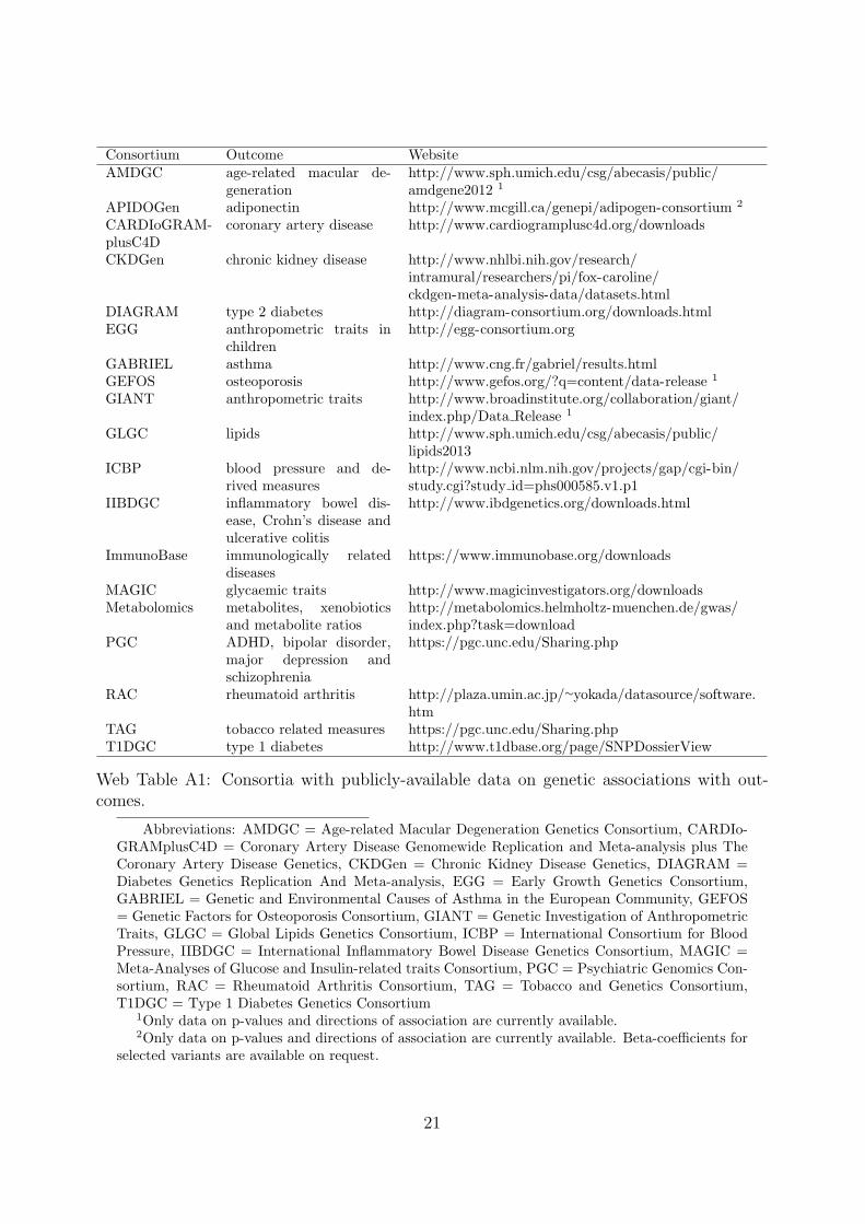
We list consortia which have made genome-wide association data publicly availableby March 2014 (Web Table A1). Some studies have released data only on the p-valuesand directions of effect of genetic variants, not the beta-coefficients. Unfortunately,such data cannot be used to estimate a causal effect parameter without making strongdistributional assumptions to derive the relevant beta-coefficients and standard errors.

Further data resources can be found (subject to registration/approval) on theNational Institute of Health (NIH) database of Genotypes and Phenotypes (dbGAP)(www.ncbi.nlm.nih.gov/gap), the European Genome–Phenome Archive (EGA) (https://www.ebi.ac.uk/ega/home), and GWAS Central (http://www.gwascentral.org/). Datafrom the Wellcome Trust Case-Control Consortium (WTCCC) consortium (http://www.wtccc.org.uk/) and the National Institute on Drug Abuse (NIDA) (https://nidagenetics.org/download data.html) is also available to bona fide researchers onrequest subject to committee approval. Many relevant datasets for cancer outcomescan be found through the International Cancer Genome Consortium (ICGC) at http://docs.icgc.org/access-raw-data.

20

Consortium Outcome WebsiteAMDGC age-related macular de-

generationhttp://www.sph.umich.edu/csg/abecasis/public/amdgene2012 1

APIDOGen adiponectin http://www.mcgill.ca/genepi/adipogen-consortium 2

CARDIoGRAM-plusC4D

coronary artery disease http://www.cardiogramplusc4d.org/downloads

CKDGen chronic kidney disease http://www.nhlbi.nih.gov/research/intramural/researchers/pi/fox-caroline/ckdgen-meta-analysis-data/datasets.html

DIAGRAM type 2 diabetes http://diagram-consortium.org/downloads.htmlEGG anthropometric traits in

childrenhttp://egg-consortium.org

GABRIEL asthma http://www.cng.fr/gabriel/results.htmlGEFOS osteoporosis http://www.gefos.org/?q=content/data-release 1

GIANT anthropometric traits http://www.broadinstitute.org/collaboration/giant/index.php/Data Release 1

GLGC lipids http://www.sph.umich.edu/csg/abecasis/public/lipids2013

ICBP blood pressure and de-rived measures

http://www.ncbi.nlm.nih.gov/projects/gap/cgi-bin/study.cgi?study id=phs000585.v1.p1

IIBDGC inflammatory bowel dis-ease, Crohn’s disease andulcerative colitis

http://www.ibdgenetics.org/downloads.html

ImmunoBase immunologically relateddiseases

https://www.immunobase.org/downloads

MAGIC glycaemic traits http://www.magicinvestigators.org/downloadsMetabolomics metabolites, xenobiotics

and metabolite ratioshttp://metabolomics.helmholtz-muenchen.de/gwas/index.php?task=download

PGC ADHD, bipolar disorder,major depression andschizophrenia

https://pgc.unc.edu/Sharing.php

RAC rheumatoid arthritis http://plaza.umin.ac.jp/∼yokada/datasource/software.htm

TAG tobacco related measures https://pgc.unc.edu/Sharing.phpT1DGC type 1 diabetes http://www.t1dbase.org/page/SNPDossierView

Web Table A1: Consortia with publicly-available data on genetic associations with out-comes.

Abbreviations: AMDGC = Age-related Macular Degeneration Genetics Consortium, CARDIo-GRAMplusC4D = Coronary Artery Disease Genomewide Replication and Meta-analysis plus TheCoronary Artery Disease Genetics, CKDGen = Chronic Kidney Disease Genetics, DIAGRAM =Diabetes Genetics Replication And Meta-analysis, EGG = Early Growth Genetics Consortium,GABRIEL = Genetic and Environmental Causes of Asthma in the European Community, GEFOS= Genetic Factors for Osteoporosis Consortium, GIANT = Genetic Investigation of AnthropometricTraits, GLGC = Global Lipids Genetics Consortium, ICBP = International Consortium for BloodPressure, IIBDGC = International Inflammatory Bowel Disease Genetics Consortium, MAGIC =Meta-Analyses of Glucose and Insulin-related traits Consortium, PGC = Psychiatric Genomics Con-sortium, RAC = Rheumatoid Arthritis Consortium, TAG = Tobacco and Genetics Consortium,T1DGC = Type 1 Diabetes Genetics Consortium

1Only data on p-values and directions of association are currently available.2Only data on p-values and directions of association are currently available. Beta-coefficients for

selected variants are available on request.

21

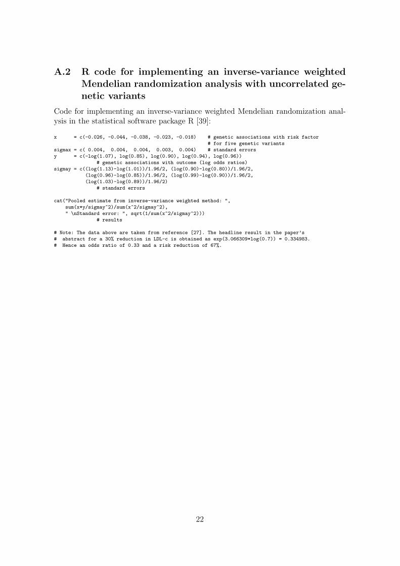
A.2 R code for implementing an inverse-variance weightedMendelian randomization analysis with uncorrelated ge-netic variants

Code for implementing an inverse-variance weighted Mendelian randomization anal-ysis in the statistical software package R [39]:

x = c(-0.026, -0.044, -0.038, -0.023, -0.018) # genetic associations with risk factor

# for five genetic variants

sigmax = c( 0.004, 0.004, 0.004, 0.003, 0.004) # standard errors

y = c(-log(1.07), log(0.85), log(0.90), log(0.94), log(0.96))

# genetic associations with outcome (log odds ratios)

sigmay = c((log(1.13)-log(1.01))/1.96/2, (log(0.90)-log(0.80))/1.96/2,

(log(0.96)-log(0.85))/1.96/2, (log(0.99)-log(0.90))/1.96/2,

(log(1.03)-log(0.89))/1.96/2)

# standard errors

cat("Pooled estimate from inverse-variance weighted method: ",

sum(x*y/sigmay^2)/sum(x^2/sigmay^2),

" \nStandard error: ", sqrt(1/sum(x^2/sigmay^2)))

# results

# Note: The data above are taken from reference [27]. The headline result in the paper’s

# abstract for a 30% reduction in LDL-c is obtained as exp(3.066309*log(0.7)) = 0.334983.

# Hence an odds ratio of 0.33 and a risk reduction of 67%.

22

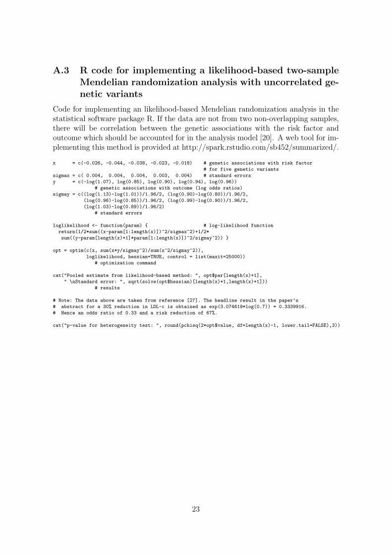
A.3 R code for implementing a likelihood-based two-sampleMendelian randomization analysis with uncorrelated ge-netic variants

Code for implementing an likelihood-based Mendelian randomization analysis in thestatistical software package R. If the data are not from two non-overlapping samples,there will be correlation between the genetic associations with the risk factor andoutcome which should be accounted for in the analysis model [20]. A web tool for im-plementing this method is provided at http://spark.rstudio.com/sb452/summarized/.







(log(0.96)-log(0.85))/1.96/2, (log(0.99)-log(0.90))/1.96/2,

(log(1.03)-log(0.89))/1.96/2)

# standard errors

loglikelihood <- function(param) { # log-likelihood function

return(1/2*sum((x-param[1:length(x)])^2/sigmax^2)+1/2*

sum((y-param[length(x)+1]*param[1:length(x)])^2/sigmay^2)) }

opt = optim(c(x, sum(x*y/sigmay^2)/sum(x^2/sigmay^2)),

loglikelihood, hessian=TRUE, control = list(maxit=25000))

# optimization command

cat("Pooled estimate from likelihood-based method: ", opt$par[length(x)+1],

" \nStandard error: ", sqrt(solve(opt$hessian)[length(x)+1,length(x)+1]))

# results

# Note: The data above are taken from reference [27]. The headline result in the paper’s

# abstract for a 30% reduction in LDL-c is obtained as exp(3.074619*log(0.7)) = 0.3339916.

# Hence an odds ratio of 0.33 and a risk reduction of 67%.

cat("p-value for heterogeneity test: ", round(pchisq(2*opt$value, df=length(x)-1, lower.tail=FALSE),3))

23

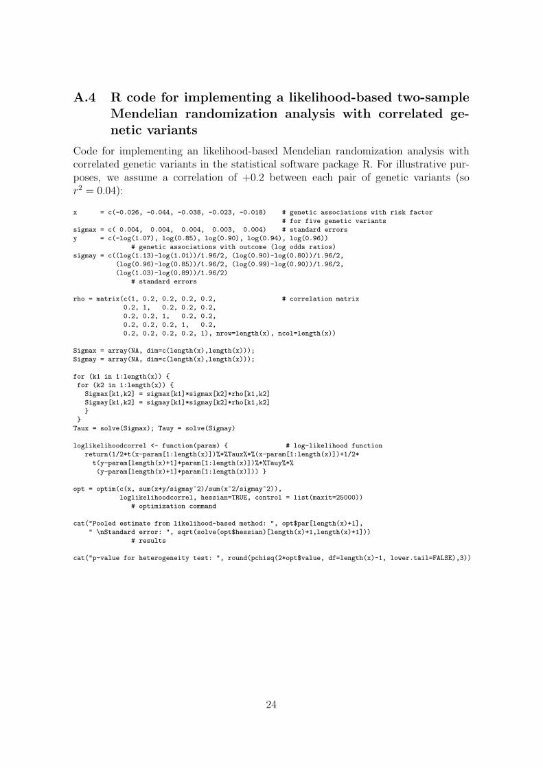
A.4 R code for implementing a likelihood-based two-sampleMendelian randomization analysis with correlated ge-netic variants

Code for implementing an likelihood-based Mendelian randomization analysis withcorrelated genetic variants in the statistical software package R. For illustrative pur-poses, we assume a correlation of +0.2 between each pair of genetic variants (sor2 = 0.04):







(log(0.96)-log(0.85))/1.96/2, (log(0.99)-log(0.90))/1.96/2,

(log(1.03)-log(0.89))/1.96/2)

# standard errors

rho = matrix(c(1, 0.2, 0.2, 0.2, 0.2, # correlation matrix

0.2, 1, 0.2, 0.2, 0.2,

0.2, 0.2, 1, 0.2, 0.2,

0.2, 0.2, 0.2, 1, 0.2,

0.2, 0.2, 0.2, 0.2, 1), nrow=length(x), ncol=length(x))

Sigmax = array(NA, dim=c(length(x),length(x)));

Sigmay = array(NA, dim=c(length(x),length(x)));

for (k1 in 1:length(x)) {

for (k2 in 1:length(x)) {

Sigmax[k1,k2] = sigmax[k1]*sigmax[k2]*rho[k1,k2]

Sigmay[k1,k2] = sigmay[k1]*sigmay[k2]*rho[k1,k2]

}

}

Taux = solve(Sigmax); Tauy = solve(Sigmay)

loglikelihoodcorrel <- function(param) { # log-likelihood function

return(1/2*t(x-param[1:length(x)])%*%Taux%*%(x-param[1:length(x)])+1/2*

t(y-param[length(x)+1]*param[1:length(x)])%*%Tauy%*%

(y-param[length(x)+1]*param[1:length(x)])) }

opt = optim(c(x, sum(x*y/sigmay^2)/sum(x^2/sigmay^2)),

loglikelihoodcorrel, hessian=TRUE, control = list(maxit=25000))

# optimization command

cat("Pooled estimate from likelihood-based method: ", opt$par[length(x)+1],

" \nStandard error: ", sqrt(solve(opt$hessian)[length(x)+1,length(x)+1]))

# results

cat("p-value for heterogeneity test: ", round(pchisq(2*opt$value, df=length(x)-1, lower.tail=FALSE),3))

24

A.5 WinBUGS code for implementing a likelihood-based two-sample Mendelian randomization analysis with uncorre-lated genetic variants

Code for implementing an likelihood-based Mendelian randomization analysis in thestatistical software package WinBUGS [40]. The WinBUGS code is recommendedfor use when there are large (more than 10) numbers of variants, and as at least asensitively analysis with fewer variants.

model {

beta1 ~ dnorm(0, 0.000001) # prior for causal effect

for (k in 1:K) { # loop over K genetic variants

xi[k] ~ dnorm(0, 0.000001) # prior for mean of G-X association

taux[k] <- pow(sigmax[k], -2) # precision of G-X association

tauy[k] <- pow(sigmay[k], -2) # precision of G-Y association

x[k] ~ dnorm(xi[k], taux[k]) # normal distribution of G-X association

eta[k] <- beta1*xi[k] # mean of G-Y association

y[k] ~ dnorm(eta[k], tauy[k]) # normal distribution of G-Y association

}

}

The WinBUGS programme can be called in R using the following code:

library(R2WinBUGS)







(log(0.96)-log(0.85))/1.96/2, (log(0.99)-log(0.90))/1.96/2,

(log(1.03)-log(0.89))/1.96/2)

# standard errors

K = 5

data <- list ("x", "y", "sigmax", "sigmay", "K")

inits <- function() {list (beta1=0)}

parameters <- c("beta1")

summarized.sim <- bugs (data, inits, parameters, "C:/foo/model.txt",

n.chains=1, n.burnin=1000, n.iter=11000, n.sims=10000, bugs.directory="C:/foo/WinBUGS14/")

cat("Pooled estimate from likelihood-based method: ", summarized.sim$summary[1,1],

" \n95% credible interval: ", summarized.sim$summary[1,3], ", ", summarized.sim$summary[1,7])

25

A.6 WinBUGS code for implementing a likelihood-based two-sample Mendelian randomization analysis with corre-lated genetic variants

Code for implementing an likelihood-based Mendelian randomization analysis in thestatistical software package WinBUGS assuming the genetic variants are correlatedin their distribution (that is, they are in linkage disequilibrium).

model {

beta1 ~ dnorm(0, 0.000001) # prior for causal effect

Tau0[1:K, 1:K] <- inverse(Sigma0[1:K, 1:K]) # variance-covariance matrix of prior

# for mean of G-X association

xi[1:K] ~ dmnorm(mu0[1:K], Tau0[1:K, 1:K]) # prior for mean of G-X association

for (k in 1:K) { eta[k] <- beta1*xi[k] } # mean of G-Y association

x[1:K] ~ dmnorm(xi[1:K], Taux[1:K, 1:K]) # multivariate normal distribution of G-X associations

y[1:K] ~ dmnorm(eta[1:K], Tauy[1:K, 1:K]) # multivariate normal distribution of G-Y associations

}

The WinBUGS programme can be called in R using the following code, whichfor illustrative purposes assumes a correlation of +0.2 between each pair of geneticvariants:

library(R2WinBUGS)







(log(0.96)-log(0.85))/1.96/2, (log(0.99)-log(0.90))/1.96/2,

(log(1.03)-log(0.89))/1.96/2)

# standard errors

K = 5; Sigma0 = diag(1, K); mu0 = rep(0, K)

rho = matrix(c(1, 0.2, 0.2, 0.2, 0.2,

0.2, 1, 0.2, 0.2, 0.2,

0.2, 0.2, 1, 0.2, 0.2,

0.2, 0.2, 0.2, 1, 0.2,

0.2, 0.2, 0.2, 0.2, 1), nrow=K, ncol=K)

Sigmax = array(NA, dim=c(K,K)); Sigmay = array(NA, dim=c(K,K));

for (k1 in 1:K) {

for (k2 in 1:K) {

Sigmax[k1,k2] = sigmax[k1]*sigmax[k2]*rho[k1,k2]

Sigmay[k1,k2] = sigmay[k1]*sigmay[k2]*rho[k1,k2]

}

}

Taux = solve(Sigmax); Tauy = solve(Sigmay)

data <- list ("x", "y", "Taux", "Tauy", "K", "Sigma0", "mu0")

inits <- function() {list (beta1=0)}

parameters <- c("beta1")

summarized.sim <- bugs (data, inits, parameters, "C:/foo/model.txt",

n.chains=1, n.burnin=1000, n.iter=11000, n.sims=10000, bugs.directory="C:/foo/WinBUGS14/")

cat("Pooled estimate from likelihood-based method: ", summarized.sim$summary[1,1],

" \n95% credible interval: ", summarized.sim$summary[1,3], ", ", summarized.sim$summary[1,7])

26

A.7 Supplementary methods for applied example

Genetic variants

Details of the genetic variants used in the applied example of the paper are givenin Web Table A2 (genetic variants in and around the CASR gene region) and WebTable A3 (genetic variants in all gene regions taken from O’Seaghdha et al. [31]). In theEPIC-InterAct study, all variants were extracted for genotyping on the Illumina 660W-Quad Bead Chip (Illumina, San Diego, CA, USA) or Illumina Cardio-Metabochip(Illumina, San Diego, CA, USA). For each variant, we give the chromosome andgene region in which the variant is located, the effect and other alleles, and thecoefficients for the genetic associations with calcium levels and fasting glucose togetherwith corresponding p-values. The associations with calcium levels are estimated inthe EPIC-InterAct dataset using linear regression with adjustment for age, sex, andcentre. The associations with fasting glucose are publicly-available data contributedby MAGIC investigators and have been downloaded from www.magicinvestigators.org.Associations with covariates in Figure 2 are also calculated in the EPIC-InterAct usinglinear regression with adjustment for age, sex, and centre. A slightly larger samplesize (up to 7311 individuals) was available for some of the covariates, depending onthe availability of data on the covariate in question (minimum sample size was 5218).

All genetic variants on the Cardio-Metabochip located within a 500kb range ofthe CASR gene region were considered for the analysis of genetic variants in andaround the CASR gene region. Proxies for the variants listed by O’Seaghdha et al.[31]) on the Cardio-Metabochip used for the analysis of genetic variants in differentgene regions were found using the SNP Annotation and Proxy Search (SNAP, http://www.broadinstitute.org/mpg/snap/ldsearch.php) [41]. Partial F statistics for thevariants in and around the CASR gene region were estimated in an analysis of variance(ANOVA) as 3.4 with 17 variants (on 17, 6314 degrees of freedom [df]), 7.9 with 6variants (on 6, 6325 df), and 30.6 with the lead variant only (on 1, 6330 df).

Genetic associations with covariates

P-values for the associations of covariates with each of the genetic variants in turnare given in Web Table A4 for variants in and around the CASR gene region, andin Web Table A5 for variants in all gene regions. We see that p-values for variantsin and around the CASR gene region are not more extreme than would be expectedby chance (3 of 17 × 13 = 221 p-values less than 0.05, minimum p-value 0.034). Incontrast, p-values for variants in different gene regions were more extreme than wouldbe expected by chance (16 of 10× 13 = 130 p-values less than 0.05, minimum p-value1× 10−13). In particular, rs780093 was associated with a large number of covariates.If this variant is omitted from the analysis using variants from different gene regions,the causal effect estimate is dominated by the variant from the CASR gene region.

27

Instrumental variable analysis methods

The likelihood-based analysis using variants from the CASR gene region was per-formed using the likelihood-based method with correlated variants in WinBUGS[42]. The matrix for the correlations between genetic variants was estimated inthe EPIC-InterAct dataset. If the individual-level data for estimating correlationswere not available, they could be estimated from the literature. A web interfacefor obtaining such correlations is the SNP Annotation and Proxy Search (SNAP;http://www.broadinstitute.org/mpg/snap/ldsearchpw.php). Normal priors with mean0 and variance 10002 were used for the parameters. The causal estimate was taken asthe posterior mean, and the 95% credible interval as the 2.5th to the 97.5th percentileof the posterior distribution.

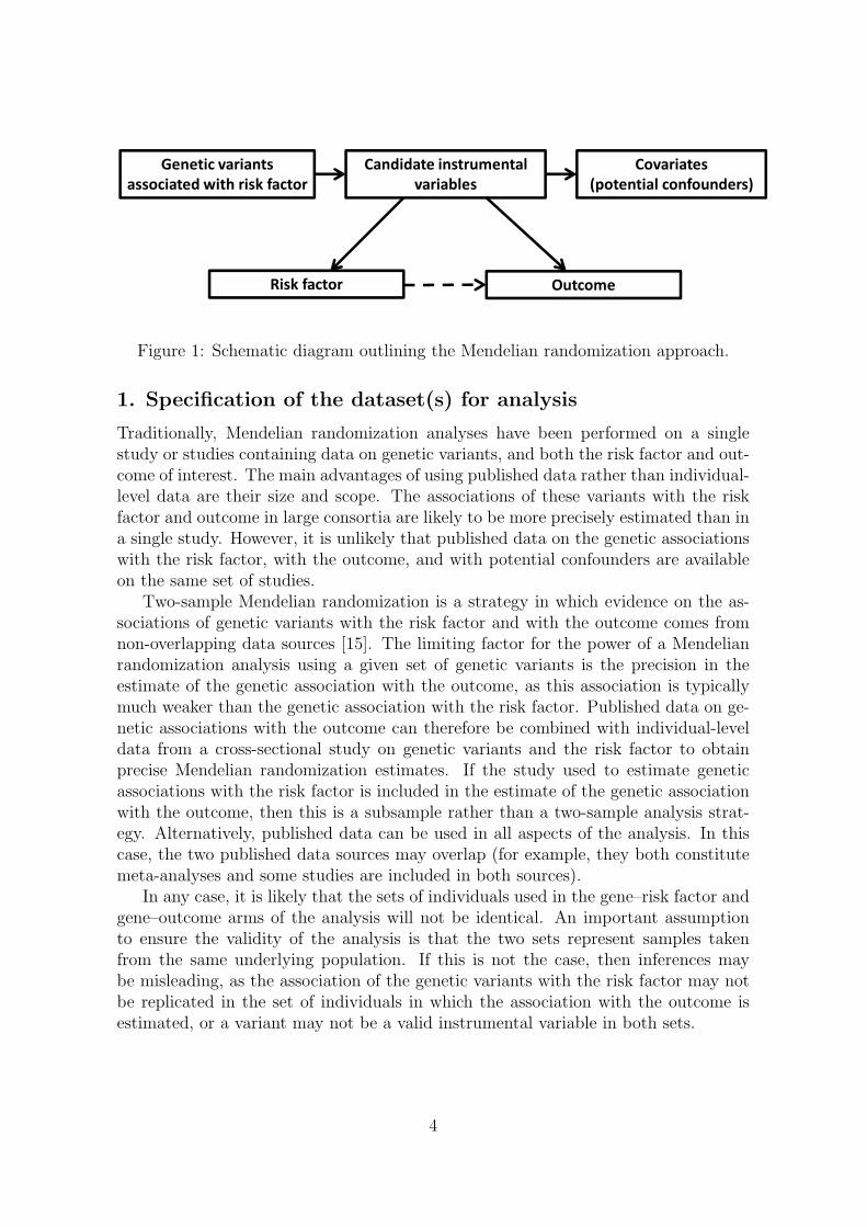
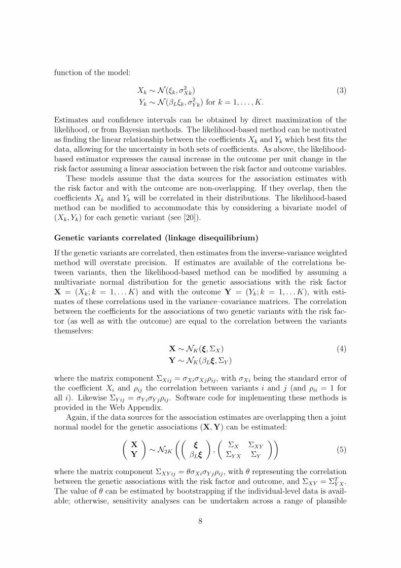
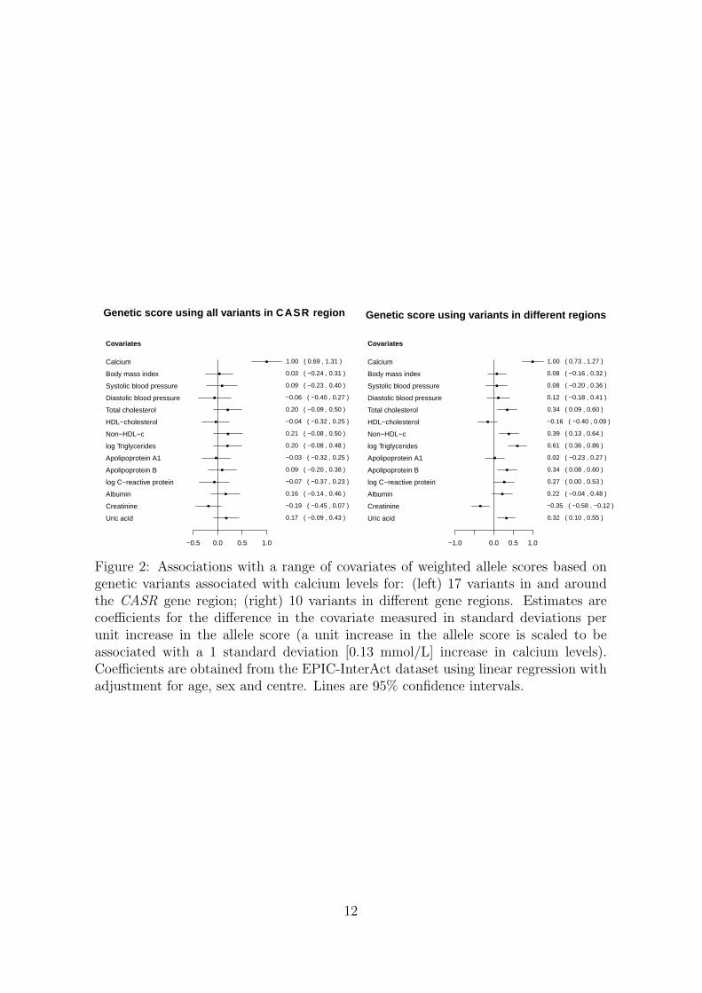
The posterior distributions of the causal effect parameter βL from the Bayesianlikelihood-based analyses using 17, 6, and 1 genetic variant are displayed in WebFigure A1. The posterior distributions are asymmetric, with longer tails in the positivethan in the negative direction.

Assessing population stratification

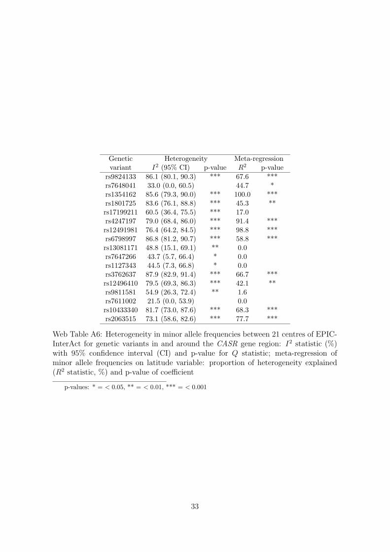
To assess population stratification, we calculated the minor allele frequencies of the17 variants in and around the CASR gene region in each of the 21 centres in EPIC-InterAct which provided data to the analysis. A meta-analysis was performed toassess whether the minor allele frequencies were similar in each centre. Additionally,the latitude of each centre was recorded by searching for the toponym in the centrename in Google Maps (www.google.com/maps) and using the lab feature “LatLngMarker”. A meta-regression was performed on the latitude variable to assess whetherdifferences in the minor allele frequencies between centres were driven by geographiclocation. Web Table A6 reports the I2 measure of the degree of heterogeneity in theminor allele frequencies, together with a 95% confidence interval for I2 and p-value forCochrane’s Q statistic, and the amount of heterogeneity accounted for by the latitudevariable in the meta-regression model (R2 statistic), together with the p-value for thelatitude coefficient in the model. We conclude that there is substantial heterogeneityin the minor allele frequencies between the centres in the EPIC-InterAct dataset, andthat the latitude of the centres explains a large proportion of this heterogeneity forseveral variants. Although this heterogeneity between centres will not lead to bias,it may indicate a latent substructure in the EPIC-InterAct and MAGIC populationsnot accounted for by the division into centres/studies, which in turn may lead to biasin the Mendelian randomization estimates.

28

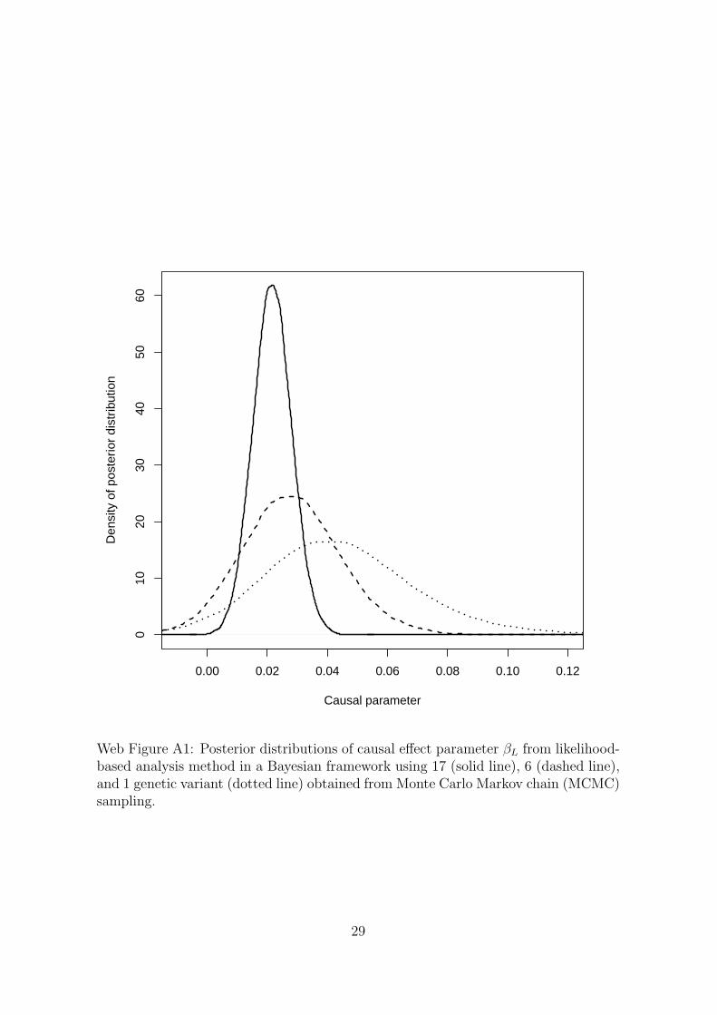
0.00 0.02 0.04 0.06 0.08 0.10 0.12

010

2030

4050

60

Causal parameter

Den

sity

of p

oste

rior

dist

ribut

ion

Web Figure A1: Posterior distributions of causal effect parameter βL from likelihood-based analysis method in a Bayesian framework using 17 (solid line), 6 (dashed line),and 1 genetic variant (dotted line) obtained from Monte Carlo Markov chain (MCMC)sampling.

29

Genetic Gene Effect Other Calcium levels Fastingvariant Chr region allele allele (mmol/L) p glucose (mM) p

rs9824133 3 IQCB1 C T 0.0062 0.007 0.0030 0.15rs7648041 3 CASR T C 0.0015 0.55 -0.0001 0.96rs1354162 3 CASR T G -0.0059 0.081 -0.0004 0.92rs1801725 3 CASR T G 0.0182 < 0.001 0.0057 0.058rs17199211 3 CASR–CSTA T C 0.0001 0.98 0.0006 0.79rs4247197 3 CASR–CSTA G A -0.0056 0.21 -0.0008 0.82rs12491981 3 CSTA C T -0.0050 0.010 0.0017 0.64rs6798997 3 CSTA–CCDC58 A G -0.0060 0.18 -0.0011 0.60rs13081171 3 CCDC58 G T -0.0033 0.72 -0.0002 0.94rs7647266 3 FAM162A T C -0.0027 0.24 0.0001 0.95rs1127343 3 FAM162A G A 0.0083 < 0.001 -0.0006 0.79rs3762637 3 KPNA1 T C -0.0026 0.44 -0.0015 0.60rs12496410 3 KPNA1 C A -0.0065 0.065 -0.0012 0.71rs9811581 3 PARP9 C T -0.0018 0.42 -0.0017 0.44rs7611002 3 PARP15–PARP14 A C 0.0012 0.73 -0.0032 0.27rs10433340 3 PARP14 A G 0.0002 0.93 -0.0012 0.59rs2063515 3 PARP14 A G -0.0013 0.64 0.0025 0.50

Web Table A2: Genetic variants in and around the calcium-sensing receptor (CASR)gene region: chromosome (Chr) and gene regions, effect and other alleles, per allele as-sociations with calcium levels (mmol/L) and fasting glucose (mM) with correspondingp-values.

Genetic Available Gene Effect Other Calcium levels Fastingvariant proxy Chr region allele allele (mmol/L) p glucose (mM) prs780093 rs780093 2 GCKR T C 0.0070 0.002 -0.0280 2× 10−38

rs838705 rs838709 2 DGKD C A 0.0033 0.19 -0.0023 0.29rs9831754 rs1355625 3 intergenic A G 0.0008 0.73 0.0056 0.008rs17251221 rs1801725 3 CASR T G 0.0182 < 0.001 0.0057 0.058rs13195786 rs4712380 6 intergenic T G 0.0009 0.72 -0.0009 0.72rs682238 rs1949365 6 intergenic A G -0.0030 0.37 0.0001 0.98rs1780159 rs12003180 9 intergenic T C -0.0121 0.029 -0.0008 0.88rs3847646 rs377765 11 intergenic T C -0.0001 0.97 -0.0021 0.33rs12150338 rs12051752 17 WDR81 T G 0.0007 0.79 -0.0031 0.18rs6091737 rs6022755 20 intergenic A C 0.0042 0.075 -0.0013 0.55

Web Table A3: Genetic variants in different gene regions: genetic variant from O’Seaghdhaet al. [31] and proxy on Cardio-Metabochip, chromosome (Chr) and gene regions, effect andother alleles, per allele associations with calcium levels (mmol/L) and fasting glucose (mM)with corresponding p-values.

30

Covariate

rs9824133

rs7648041

rs1354162

rs1801725

rs17199211

rs4247197

rs12491981

rs6798997

rs13081171

rs7647266

rs1127343

rs3762637

rs12496410

rs9811581

rs7611002

rs10433340

rs2063515

BMI

0.24

0.47

0.35

0.64

0.62

0.90

0.76

0.71

0.97

0.65

0.89

0.58

0.29

0.74

0.69

0.13

0.07

SBP

0.27

0.35

0.66

0.63

0.05

0.78

0.46

0.25

0.82

0.14

0.37

0.78

0.28

0.14

0.38

0.64

0.15

DBP

0.36

0.32

0.46

0.98

0.14

0.39

0.39

0.52

0.37

0.11

0.48

0.75

0.44

0.24

0.16

0.70

0.84

Totalch

ol

1.00

0.90

0.74

0.41

0.86

0.46

0.58

0.28

0.25

0.92

0.31

0.79

0.04

0.58

0.87

0.95

0.23

HDL-c

0.39

0.97

0.31

0.51

0.97

0.46

0.46

0.61

0.51

0.14

0.45

0.96

0.10

0.17

0.65

0.74

0.20

Non-H

DL-c

0.80

0.92

1.00

0.31

0.82

0.65

0.79

0.36

0.19

0.71

0.21

0.77

0.16

0.92

0.99

0.96

0.11

logTrig

0.27

0.74

0.88

0.15

0.58

0.88

0.91

0.43

0.23

0.56

0.10

0.63

0.26

0.37

0.98

1.00

0.83

ApoA1

0.54

0.65

0.19

0.60

0.96

0.57

0.51

0.66

0.80

0.37

0.42

0.86

0.11

0.20

0.97

0.40

0.31

ApoB

0.33

0.87

0.88

0.55

0.52

0.91

0.92

0.43

0.36

0.83

0.56

0.98

0.39

0.86

0.84

0.65

0.05

logCRP

0.97

0.20

0.70

0.77

0.59

0.72

0.69

0.60

0.62

0.92

0.29

0.70

0.61

0.64

0.65

0.55

0.86

Albumin

0.12

0.87

0.86

0.73

0.84

0.56

0.41

0.35

0.77

0.76

0.48

0.26

0.65

0.51

0.60

0.51

0.74

Creatin

0.99

0.57

0.14

0.18

0.71

0.11

0.13

0.23

0.35

0.72

0.61

0.28

0.36

0.50

0.10

0.96

0.75

Uricacid

0.53

0.44

0.79

0.37

0.63

0.88

0.79

0.55

0.52

0.89

0.11

0.57

0.35

0.37

0.03

0.95

0.30

Web

Tab

leA4:

P-values

forassociationsof

covariates

withallgenetic

varian

tsin

andarou

ndtheCASR

generegion

.P-values

less

than

0.05

areshow

nin

boldface.

31

Covariate

rs78

0093

rs83

8709

rs13

5562

5rs1801

725

rs47

1238

0rs19

4936

5rs120

0318

0rs37

7765

rs120

5175

2rs60

2275

5Bodymassindex

0.14

0.74

0.11

0.64

0.17

0.56

0.46

0.34

0.22

0.28

Systolic

bloodpressure

0.56

0.95

0.43

0.63

0.89

0.90

0.94

0.13

0.20

0.18

Diastolic

bloodpressure

0.78

0.46

0.15

0.98

0.84

0.51

0.81

0.23

0.76

0.09

Totalcholesterol

<0.001

0.98

0.27

0.41

0.39

0.32

0.90

0.44

0.02

0.45

HDL-cholesterol

0.02

0.70

0.37

0.51

0.13

0.81

0.08

0.49

0.11

0.48

Non

-HDL-c

<0.001

0.93

0.16

0.31

0.18

0.30

0.47

0.31

0.09

0.31

logTriglycerides

<0.001

0.87

0.50

0.15

0.15

0.01

0.38

0.73

0.15

0.15

Apolipop

rotein

A1

0.67

0.72

0.55

0.60

0.19

0.59

0.14

0.46

0.15

0.98

Apolipop

rotein

B<

0.001

0.86

0.15

0.55

0.23

0.48

0.86

0.19

0.15

0.15

logC-reactiveprotein

<0.001

0.04

0.03

0.77

0.58

0.54

0.95

0.53

0.69

0.02

Albumin

0.05

0.64

0.91

0.73

0.50

0.25

0.49

0.50

0.86

0.32

Creatin

<0.001

0.39

0.45

0.18

0.02

0.23

0.91

0.53

0.58

0.03

Uricacid

<0.001

0.34

0.32

0.37

0.38

0.39

0.67

0.18

0.17

0.82

Web

Tab

leA5:

P-values

forassociationsof

covariates

withgenetic

varian

tsin

differentgeneregion

s.P-values

less

than

0.05

areshow

nin

boldface.

32

Genetic Heterogeneity Meta-regressionvariant I2 (95% CI) p-value R2 p-value

rs9824133 86.1 (80.1, 90.3) *** 67.6 ***rs7648041 33.0 (0.0, 60.5) 44.7 *rs1354162 85.6 (79.3, 90.0) *** 100.0 ***rs1801725 83.6 (76.1, 88.8) *** 45.3 **rs17199211 60.5 (36.4, 75.5) *** 17.0rs4247197 79.0 (68.4, 86.0) *** 91.4 ***rs12491981 76.4 (64.2, 84.5) *** 98.8 ***rs6798997 86.8 (81.2, 90.7) *** 58.8 ***rs13081171 48.8 (15.1, 69.1) ** 0.0rs7647266 43.7 (5.7, 66.4) * 0.0rs1127343 44.5 (7.3, 66.8) * 0.0rs3762637 87.9 (82.9, 91.4) *** 66.7 ***rs12496410 79.5 (69.3, 86.3) *** 42.1 **rs9811581 54.9 (26.3, 72.4) ** 1.6rs7611002 21.5 (0.0, 53.9) 0.0rs10433340 81.7 (73.0, 87.6) *** 68.3 ***rs2063515 73.1 (58.6, 82.6) *** 77.7 ***

Web Table A6: Heterogeneity in minor allele frequencies between 21 centres of EPIC-InterAct for genetic variants in and around the CASR gene region: I2 statistic (%)with 95% confidence interval (CI) and p-value for Q statistic; meta-regression ofminor allele frequencies on latitude variable: proportion of heterogeneity explained(R2 statistic, %) and p-value of coefficient

p-values: * = < 0.05, ** = < 0.01, *** = < 0.001

33

Documents

Using published data in Mendelian randomization: a blueprint for efficient identification of causal risk factors