Utility-based Regression

Luis Torgo1 and Rita Ribeiro2

1 LIACC-FEP, University of Porto, R. Ceuta, 118, 6., 4050-190 Porto, Portugalltorgo@liacc.up.pt,

WWW home page: http://www.liacc.up.pt/~ltorgo2 LIACC, University of Porto, R. Ceuta, 118, 6., 4050-190 Porto, Portugal

rita@liacc.up.pt

Abstract. Cost-sensitive learning is a key technique for addressing manyreal world data mining applications. Most existing research has been fo-cused on classification problems. In this paper we propose a frameworkfor handling regression problems in applications with non-uniform costsand benefits across the domain of the continuous target variable. Namely,we describe two metrics for asserting the costs and benefits of the pre-dictions of any model given a set of test cases. These two measures to-gether or individually, provide a more informed assessment of the utilityof any regression model given the application-specific preference biases.We illustrate the use of our metrics in the context of a specific type ofapplications where non-uniform costs are required: the prediction of rareextreme values of a continuous target variable. Our experiments provideclear evidence of the utility of the proposed framework in the context ofthis class of regression problems.

1 Introduction

In many real world applications of data mining the costs and benefits of us-ing prediction models are non-uniform. These observations have motivated thework on cost-sensitive learning (e.g. [5, 7]) and more generally on utility-basedmining [17, 19]. In the context of applying the discovered knowledge under anon-uniform cost setup, most works have focused on classification tasks (e.g. [5–8, 11, 12]). Still, within numeric prediction problems, also know as regression,similar problems arise. However, as mentioned by Crone et. al. [4] most workson regression assume uniform costs and use some form of average error statis-tic. In this context, several authors (e.g. [1, 2, 4, 9]) have proposed new cost oferror functions that try to address these issues. However, most of these worksonly consider one particular type of non-uniform costs of errors: the differencebetween under- and over-predictions, i.e. situations where the predicted valuesare above or below the true values, respectively.

This paper proposes a framework for evaluating regression models in the con-text of arbitrarily shaped costs and benefits across the domain of the numerictarget variable of regression tasks. We propose two new evaluation metrics thatincorporate the notions of costs and benefits and thus are able to provide bet-ter feedback on the merits of regression models in the context of the specific

biases of any numeric prediction task. These metrics use cost and benefit sur-faces that we also formalize, which can be regarded as continuous versions of thewell-know notion of misclassification cost matrices. We illustrate the use of ourproposed metrics in a particular class of non-uniform costs/benefits application:the prediction of rare extreme values of a continuous variable.

2 Problem Formulation

Predictive learning tries to obtain an approximation of an unknown functionf : χ → γ, based on a training data set D drawn from a distribution with domainχ × γ, where χ is the domain of the set of predictor variables and γ is either adiscrete domain in the case of classification tasks, or ℜ in the case of regression.The obtained approximation, fβ , is a model with a set of parameters, β, thatare obtained by optimizing some preference criterion. For classification, this isusually the error rate, while in the case of regression there are more alternatives,but the most frequent are the mean squared error, 1

n

∑ni=1 (yi − yi)

2, or the

mean absolute deviation, 1n

∑ni=1 |yi − yi|.

Many authors (e.g. [5, 7]) have noticed the problems arising from the uni-form cost assumption of the error rate evaluation criterion. This assumption isunacceptable for many real world domains. The cost matrix formulation over-comes these limitations by allowing the specification of the cost of misclassifyingclass i by class j, and leads to the criterion of expected cost minimization,1n

∑ni=1 C(y, y), where C(y, y) is an entry on the pre-specified cost matrix.

Regards regression few authors have addressed the issue of differentiatedcosts. Most of the existing works on having non-uniform costs for regressionhave been addressing the issue of differentiating the cost of under-predictions(y < y), from the cost of over-predictions (y > y) (e.g. [1, 4]). This is the case ofthe LINLIN cost function defined as follows,

LINLIN =

co|y − y| for y > y

0 for y = y

cu|y − y| for y < y

(1)

where co and cu are constants for penalizing over- and under-predictions, respec-tively.

The LINLIN cost function allows to differentiate the cost of the errors de-pending on where they occur, namely an error with amplitude 4 may be morepenalized than another error with the same amplitude if both occur on differ-ent “sides” of the true value, provided the constants co and cu are different.Although these approaches address several important application-specific re-quirements, they are special cases of a more general definition of costs acrossall combinations of true and predicted values. Moreover, they do not allow tohandle some cases that are very relevant in other applications. For instance, instock market forecasting, predicting a future price change of -1% for a true valueof 1%, has the same error amplitude as predicting 6% for a true value of 8%.The two cases are under-predictions, and thus would have the same cost using

the LINLIN metric1. However, these two situations are completely differentfrom an investor’s perspective. While the first prediction could lead to a sellaction that would in effect result in a loss of money, the latter would lead to acorrect and profitable action. These problems arise because all these measureslook at the error amplitudes independently of where they occur in the range ofthe target variable. As mentioned by Torgo [15], for this type of applications itis important to study the performance of the models as a function of the targetvariable range. In this paper we propose to address this issue by associating toeach prediction a cost that is dependent on a user-defined relevance of both thetrue and predicted values.

3 Utility-Based Regression

As mentioned by Zadrozny [18], research on cost-sensitive learning has tradi-tionally been formalized in terms of costs as opposed to benefits or rewards.However, evaluating a model in terms of benefits is generally preferable becausethere is a natural baseline from which to measure all benefits whether positive(real benefits of a prediction) or negative (that are in effect costs) [7]. Our pro-posal follows these lines, by measuring the utility of a regression model throughthe total balance between the costs and rewards originated by its predictions.

We assume that for some applications the relevance (importance) of thevalues of the target variable is not uniform across its domain. This domain-dependent information shall be provided through the specification of a relevancefunction, φ(Y ) : ℜ → 0..1, that maps the domain of the target variable intoa 0..1 scale of relevance, where 1 represents maximum relevance. Our proposaldoes not depend on any particular shape of the φ() function. We assume thisfunction is specified by the user using his/her domain knowledge. The specifica-tion of the relevance function is the step of our proposal that is most challengingfor the user. Given the large range of applications where the relevance of thetarget variable is non-uniform, it is virtually impossible to describe reasonabledefault relevance functions for all these applications. Still, in many applicationsrelevance is often associated with rarity (e.g. highly profitable customers; highvariations on stock prices; extreme weather conditions, etc.). For these appli-cations relevance can be defined as a function that is inversely proportionalto the probability density function (pdf) of the values of the target variable.Although obtaining the functional form of these pdf’s is generally non trivial,reasonable approximations based on the available data samples can be obtainedwith techniques like kernel density approximators (e.g. [10]). In Section 4 we usea related strategy to derive a relevance function to be used in the context of aclass of applications where relevance is associated with rarity: the prediction ofrare extreme values of the target variable.

Generally, the cost of a prediction depends not only on the relevance of thetest case value but also on the relevance of the predicted value. In effect, allthree following situations are penalizing in a cost-sensitive application:

1 And also using the other “standard” error metrics like MSE, for instance.

1. Wrongly predict a relevant value for an irrelevant test case (kind of falsealarm);

2. Predict an irrelevant value for a relevant test case (also known as opportunitycosts);

3. Predict a relevant but very different value for a relevant test case (the mostserious mistakes: confusing relevant events).

We capture this notion of relevance of the prediction for a given test case bymeans of the definition of a bi-variate relevance function, Φ(Y , Y ), that dependson the relevance of both the true and predicted values,

Φ(Y , Y ) = (1 − m) · φ(Y ) + m · φ(Y ) (2)

This function is a simple weighted average of the individual relevance of theY and Y values. It is maximum when both are highly relevant and these arethe cases where the cost of the predictions may reach the maximum if theyare not accurate enough. The m parameter (0 ≤ m ≤ 1) differentiates betweensituations 1 (false alarms) and 2 (opportunity costs). Setting m > 0.5 makes thelatter more important.

The cost of a prediction should also depend on its precision, i.e. how nearare Y and Y from each other. Moreover, it should also be possible for the userto establish some kind of application-specific measure of cost in whatever unitsmake sense for the domain. In this context, we define the cost of a prediction fora test case as follows,

c(Y , Y ) = Φ(Y , Y ) × Cmax × L(Y , Y ) (3)

where Cmax is the maximum cost that is only assigned when the relevance of theprediction is maximum (i.e. Φ(Y , Y ) = 1); and L(Y , Y ) is a loss function thatmeasures the prediction error.

The term Φ(Y , Y ) × Cmax can be seen as a kind of case-specific maximumcost value. This is the maximum penalty we get if Y is the “worst possible”prediction for the test case under consideration.

With respect to the loss function we could in principle use any metric func-tion, like for instance the absolute deviation of the values, i.e. |Y −Y |. However,in order to make the meaning of the value c(Y , Y ) more intuitive, we recom-mend the use of a percentage-type loss function that ranges from 0 to 1. Suchfunction will then represent the proportion of the case-specific maximum costwe get due to our prediction. For maximum error (L(Y , Y ) = 1) we get the fullpenalty of the particular test case (Φ(Y , Y ) × Cmax), while a perfect prediction(L(Y , Y ) = 0) would entail no cost as expected. This means the value of c(Y , Y )will be expressed in the same units as Cmax, which is provided by the user, andthus it is more intuitive for him/her. In this context, we propose the followingloss function that ranges from 0 to 1:

L(Y , Y ) = | maxi∈ Y ..Y

φ(i) − mini∈ Y ..Y

φ(i)| (4)

The use of the maximum and minimum functions is due to the fact that wewant to let the user specify any arbitrarily shaped φ() function. This means thatwe can have two quite different Y values with the same value of φ(), which wouldlook like a perfect prediction if we had used the difference of relevances directly.However, these cases are exactly the most serious mistakes we want to avoid(the 3rd case on the list presented before), because we are “confusing” betweentwo quite different but very relevant events, and thus we have at the same timea false alarm and an opportunity cost. In order to avoid this effect, we use thedifference between the maximum and minimum relevance in the interval betweenthe true and predicted values. If both values have high relevance but are quitedifferent then surely there will be values in between with lower relevance andthis will result in a higher value of our loss function.

The function c() can be seen as a continuous version of cost matrices, i.e. acost surface. Using this function we can calculate the total cost of the predictionsof a regression model using,

TC =

n∑

i=1

c(yi, yi) (5)

In [16] we proposed a related statistic, RExE, in the context of a specificcase of non-uniform costs application: the prediction of rare extreme values of acontinuous variable. Compared to this previous work, we extend it by consideringa broader class of applications by means of the notion of relevance function, whichhas lead to a different definition of cost surfaces. Moreover, we will also considerthe benefits of the predictions that were not taken into account on this previouswork. In effect, the extensive set of experiments we have carried out before haveshown a few counter-intuitive model rankings that have motivated the use ofbenefits. Namely, when opportunity costs are not very large when compared tothe cost of false alarms, and when events with very large relevance are quite rarewhen compared to the bulk of data, we have observed that very “conservative”models2 were not being sufficiently penalized. This is particularly serious forseveral applications like for instance the prediction of the future changes in stockprices. A model that predicts the most frequent change, which is approximatelyzero, achieved a relatively low total cost of its predictions because large variationsof the price are extremely rare and thus there are few opportunity costs. Becausethese models never predict relevant values, they never suffer from costs associatedto false alarms or confused events, and thus their total cost of predictions islow as it amounts to the rare opportunity costs. As such, this type of modelswere constantly being ranked high in terms of comparisons using a metric basedsolely on costs of predictions. However, these models are completely useless forthis application as their predictions are not actionable (and thus non-profitable)because they always predict a price change near zero. This means that havingmodels with a low value of total cost of predictions may not be enough for some

2 Models that always predicted very frequent but irrelevant values.

application setups, particularly if this associated with missing all relevant valuesof the target variable.3

In this context, we also propose to evaluate the benefits of the predictionsof a model. The goal here is to assert the ability of the model to capture (i.e.accurately predict) most of the relevant values in a test set. In the case of benefitsit is only the relevance of the true value that counts, i.e. we are interested inasserting how well a model predicts the test cases that are relevant. As such, thebenefit surface is defined as,

b(Y , Y ) = φ(Y ) × Bmax × (1 − L(yi, yi)) (6)

where Bmax is a user-defined maximum reward that is supposed to be measuredin the same units as the previously used Cmax constant; and L() is a loss functionwith range 0..1 (e.g. the one defined in Equation 4).

Note that our definition of benefits implicitly associates higher rewards withhigher relevance. The term φ(Y )×Bmax calculates the case-specific benefit, whilethe last term in Equation 6 is the proportion of this reward that we get with ourprediction.

As before, we can also calculate the total benefits of the predictions of aregression model by,

TB =

n∑

i=1

b(yi, yi) (7)

Having defined the total costs and benefits of the predictions of a model wedefine the utility of the model as the net balance between these two quantities,

U = TB − TC (8)

The use of this metric only makes sense if TC and TB are measured onthe same units and are somehow comparable. This is related to the values usedfor Cmax and Bmax. These two constants should be set with values of somequantity that makes sense for the application being addressed (e.g. monetaryunits). In spite of the validity of the U metric we think that showing the valuesof the 3 measures (U , TC and TB) is always more informative than using onlythe value of U , because different users may have different balances between theimportance of what is being measured by TC and TB. Moreover, it is alsoconceivable that for some applications some form of weighted average of TC andTB may actually make more sense than this simple balance we are proposing.Still, the most important issue is to accurately measure the costs and benefitsof the predictions of a model according to the application preference biases.

3 This argumentation has strong resemblance with the need of evaluating classificationmodels with both precision and recall in typical information retrieval setups.

4 An Illustrative Application

Modeling extreme data is very important in several application domains, like forinstance finance, meteorology, ecology, etc.. Several of these applications involvepredicting a continuous variable. For these domains the extreme (high or low)values of the target variable are much more important than the others. More-over, these extremes are generally quite rare, which turns this into a very hardprediction problem with very clear non-uniform costs and benefits of predictions.In this section we illustrate the use of our proposed framework for utility-basedregression in the context of this class of applications. We apply our metrics in acomparison between quite diverse modelling techniques on a real world data setwhere the prediction of rare extreme values is of primary importance.

The application we use to illustrate our proposal concerns stock market fore-casting. Namely, the data are about the task of trying to predict the future dailyvariation in closing prices of the IBM stock, using information regarding the val-ues of these variations on the 10 previous market sessions. The data set consistsof information on 8166 daily market sessions (roughly 30 years), each being de-scribed by 10 predictor variables (the variations on the 10 previous days) and atarget variable (the variation on the next day). This application is a very clearexample of non-uniform costs (and benefits) of predictions. In effect, any modelthat is extremely accurate at predicting small price variations (the most com-mon) is essentially useless for a trader. Profitable trading is based on being ableto capitalize on large price changes. Trades carried out over small price changesare usually not able to cover the trading costs and thus are non-profitable oreven represent a loss of money. As such, in these applications the accuracy onthe relevant (i.e. extreme high or low) changes of prices is the key criterion.

In order to apply our evaluation method we need to specify a relevance func-tion for this domain. As mentioned before, in this class of applications relevanceis strongly associated with extreme and rare values of the target variable. More-over, for our concrete application the distribution of the target variable has anormal-like shape with very marked tails (the rare extreme variations). Fromthe description of the goals of this application it should be clear that the rele-vance function should have a shape that is inverse of the probability distributionfunction of the price variations. We now describe a general method that obtainsan approximation of this function, and that can be used in any application thatshares the same objectives.

Box plots [3] are graphical displays of a data set that are often used to pro-vide a summary of the distribution of a continuous variable, including signalingpotential outliers. In the context of box plots, outliers are defined as values aboveor below the so-called adjacent values. If r is the inter-quartile range defined asthe difference between the 3rd and 1st quartiles of the target variable, then theupper adjacent value, adjH , is defined as the largest observation that is less orequal to the 3rd quartile plus 1.5r. Equivalently, the lower adjacent value, adjL,is defined as the smallest observation that is greater or equal to the 1st quartileminus 1.5r. Given the definition of these adjacent values it is obvious that mostof the data lies in the interval between these two values. We could use these

two thresholds to set two rigid limits above (or below) which all values wouldbe considered rare extremes and thus highly relevant. Instead of rigid limits wepropose to use a sigmoid-like function for establishing a smooth relevance func-tion. However, this function uses the information of the adjacent values to setupthe shape of the sigmoid so has to reflect the information provided by box plotsconcerning the distribution of the variable.

A sigmoid function is defined by two parameters, c and s, which control itsshape. Our relevance function is defined as follows:

φ(Y ) =

{

c1

c1+es1·Y , Y ≤ Yc2

c2+es2·Y , Y > Y(9)

where Y is the sample median of variable Y and c1, c2, s1 and s2 are shaperelated parameters that are to be set as follows,

c1 = exa·log 1/3

xa−xb c2 = exc·log 1/3

xc−xd

s1 = log 1/3xa−xb

s2 = log 1/3xc−xd

φ(xa) = φ(xc) = 0.5 φ(xb) = φ(xd) = 0.25

The x values are then selected in the following way,

xa = adjL(Y ) xb = adjL(Y ) + k · mxc = adjH(Y ) xd = adjH(Y ) − k · m

m = |Y −(adjL(Y )+i)|+|Y −(adjH(Y )−d)|2

i = adjL(Y ) · adjL−min(Y )

Y −min(Y )d = adjH(Y ) · adjH (Y )−Y

max(Y )−Y

where 0 ≤ k ≤ 1 is a constant that controls the acceleration of the sigmoidfunction around its mid-point (φ(Y ) = 0.5).

Figure 1 provides a graphical illustration of the quantities involved in thederivation of the relevance function we have just described. This figure showsthe box plot of an arbitrary normal-like distribution and the respective sigmoid-based relevance function obtained according to Equation 9.

The relevance function is defined using distribution properties of the targetvariable (min(Y ), adjL(Y ), Y , adjH(Y ) and max(Y )) that can be easily esti-mated from the available data sample. This function can be generally applied onproblems where the target variable has a normal-like shape and where relevanceis associated to rare extremes. This function provides a smooth variation of therelevance values across the domain of the target variable, and can be seen as agood approximation of the idea of an inverse function of the pdf of the targetvariable (c.f. Section 3).

The other three parameters necessary to use our U metric are Cmax, Bmax

and m. Given our absence of domain expertise on stock market trading we haveset these parameters using what seemed to us reasonable settings. Namely, we

min(Y) adjL Y~ adjH max(Y)

box−plot

0.0

0.2

0.4

0.6

0.8

1.0

Relevance Mapping

xa xb Y~ xd xc

Rel

evan

ce (

φ)

Fig. 1. A sigmoid-based relevance function for rare extreme values prediction.

decided that the maximum benefit should be clearly higher than the maximumcost to try to reward proactive models. In our experiments we have used Cmax =10 and Bmax = 20. With respect to the m parameter we have set it to 0.5, i.e.equal importance to false alarms and opportunity costs.

−0.2

−0.1

0.0

0.1

−0.2

−0.1

0.0

0.1

0

2

4

6

8

Cost Surface ibm

yy

c0.5

−0.2

−0.1

0.0

0.1

−0.2

−0.1

0.0

0.1

5

10

15

Benefit Surface ibm

yy

b0.5

Fig. 2. The cost and benefit surfaces for the IBM data set.

Having set all necessary parameters we can get a better idea of the biasesintroduced by our method by looking at the shapes of the resulting cost andbenefit surfaces for the IBM data, which are shown on Figure 2. The surfaceshelp us to understand the risk associated with a prediction of a relevant valuethat may lead us to the higher rewards but may also lead to the higher costs ifit is not accurate. More conservative models do not take such higher risks, buton the other hand can not “reach” the more profitable predictions.

In order to test our proposed metrics under different experimental setupswe have applied 3 quite different modeling techniques to the IBM data set.Namely, regression trees, neural networks and support vector machines. For all3 methods we have used their implementations freely available on the R softwareenvironment [13], more specifically the function rpart() of the package rpart,the function nnet() of the package nnet and the function svm() of the packagee1071. All 3 methods were used without any extensive parameter tuning asthe goal was not to achieve the best possible accuracy but instead to test anevaluation metric under different setups. With respect to regression trees wehave used rpart() with cp=0 and with post-pruning using the 1-SE rule. Neuralnetworks were obtained using the function nnet() with parameters linout=T,size=min(10,ncols(data)/2), decay=0.01 and maxit=500. Regards supportvector machines we have use the settings cost=500 and gamma=0.03 for thefunction svm(). As a baseline “dummy” model we have also evaluated the resultsof always predicting the median value of the target variable. In the context ofthis particular application this can be regarded as the worse possible solution asit leads to zero trading and thus null profit.

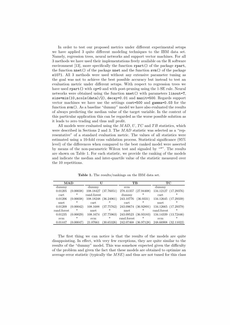
All models were evaluated using the MAD, U , TC and TB statistics, whichwere described in Sections 2 and 3. The MAD statistic was selected as a “rep-resentative” of a standard evaluation metric. The values of all statistics wereestimated using a 10-fold cross validation process. Statistical significance (95%level) of the differences when compared to the best ranked model were assertedby means of the non-parametric Wilcox test and signaled by “*”. The resultsare shown on Table 1. For each statistic, we provide the ranking of the modelsand indicate the median and inter-quartile value of the statistic measured overthe 10 repetitions.

Table 1. The results/rankings on the IBM data set.

MAD U TB TC

dummy dummy svm dummy0.01205 (0.00038) 108.18427 (37.76051) 278.41357 (27.94408) 134.12127 (17.29376)

cart * rand.forest dummy * cart *0.01206 (0.00038) 108.18248 (36.24961) 243.10776 (36.9331) 134.12645 (17.29339)nnet * cart * cart * nnet *

0.01209 (0.00042) 108.1688 (37.75762) 243.09674 (36.92891) 134.12665 (17.29379)rand.forest * nnet * nnet * rand.forest *

0.01235 (0.00029) 108.1674 (37.75963) 243.09523 (36.93183) 134.14339 (13.72446)svm * svm * rand.forest * svm *

0.01447 (0.00047) 21.07661 (30.65326) 242.07468 (36.97128) 248.66908 (32.11022)

The first thing we can notice is that the results of the models are quitedisappointing. In effect, with very few exceptions, they are quite similar to theresults of the “dummy” model. This was somehow expected given the difficultyof the problem and given the fact that these models are obtained to optimize anaverage error statistic (typically the MSE) and thus are not tuned for this class

of applications. Ribeiro and Torgo [14] have shown that modeling techniquesspecialized for the goals of these applications can make a clear difference.

The use of our metrics revealed some interesting information that could notbe observed from looking at the MAD scores. In effect, we can see that the SVMfollows a quite different approach to this prediction task. Namely, we can observethat it achieves a much higher score in terms of benefits, clearly indicating a morerisky approach to the prediction problem. However, this approach also has leadto a higher value of TC, and as a result a poor score in terms of net balance(U score). Still, given the fact that there was no particular tuning of the modelparameters, we can say that the SVM is probably a model where more timeshould be invested in the context of this application, so that the signals it isproducing get more precise.

5 Conclusions

This paper has described a new evaluation framework for regression tasks withnon-uniform costs and benefits of the predictions. Based on the existing workon cost-sensitive classification we have proposed an extension of this learningapproach to numeric prediction tasks.

Our proposal is based on the specification of a relevance function over thedomain of the target continuous variable. This function is the basis of the defi-nitions of cost and benefit surfaces that can be regarded as continuous versionsof cost/benefit matrices used in classification tasks. The use of the relevancefunction relieves the user from the heavy burden of having to specify a cost(and benefit) for all points in the bi-dimensional space of the predicted and truetarget values. The total cost and benefit of the predictions of a model provide,either individually or aggregated on an utility measure, important insights onthe predictive performance of a model. Moreover, these insights are related tothe application goals in terms of what is really relevant.

We have illustrated the use of our evaluation framework in the context of aparticular class of applications: the prediction of rare extreme values of a con-tinuous variable. Namely, we have used a data set from stock market predictionto introduce a general relevance function that is biased towards the goals ofthis class of applications. Using the resulting cost an benefit surfaces we havecompared three different models on this data set. The results of our experimentshave revealed important aspects of the predictive performance of the differentmodels.

Overall, our proposal fulfills the goals of having a framework for utility-basedregression that can be used in many real world applications. This proposal clearlyincreases the applicability of cost-sensitive learning by extending it to numericalprediction tasks.

In future we plan to extend the experimental evaluation of our proposal andalso to plug in the U metric in the model development stages so as to obtainmodels that optimize the utility instead of prediction error.

References

1. P. Christoffersen and F. Diebold. Further results on forecasting and model selectionunder asymmetric loss. Journal of Applied Econometrics, 11:561–571, 1996.

2. P. Christoffersen and F. Diebold. Optimal prediction under general asymmetricloss. Econometric Theory, 13:808–817, 1997.

3. W. Cleveland. Visualizing data. Hobart Press, 1993.4. S. Crone, S. Lessmann, and R. Stahlbock. Utility based data mining for time

series analysis - cost-sensitive learning for neural networks. In G. Weiss, M. Saar-Tsechansky, and B. Zadrozny, editors, Proceedings of the 1st International Work-shop on Utility-Based Data Mining, pages 59–68, 2005.

5. P. Domingos. Metacost: A general method for making classifiers cost-sensitive. InProceedings of the 5th International Conference on Knowledge Discovery and DataMining (KDD-99), pages 155–164. ACM Press, 1999.

6. C. Drummond and R. Holte. Exploiting the cost of (in)sensitivity of decision treesplitting criteria. In Proc. 17th International Conf. on Machine Learning, pages239–246. Morgan Kaufmann, San Francisco, CA, 2000.

7. C. Elkan. The foundations of cost-sensitive learning. In Proceedings of 7th IJ-CAI’01, pages 973–978, 2001.

8. W. Fan, S. Stolfo, J. Zhang, and P. Chan. AdaCost: misclassification cost-sensitiveboosting. In Proc. 16th International Conf. on Machine Learning, pages 97–105.Morgan Kaufmann, San Francisco, CA, 1999.

9. C. Granger. Predition with a generalized cost of error function. Operational Re-search Quarterly, 20:199–207, 1969.

10. W. Hardle. Applied Nonparametric Regression. Cambridge University Press, 1990.11. M. Kukar and I. Kononenko. Cost-sensitive learning with neural networks. In

European Conference on Artificial Intelligence, pages 445–449, 1998.12. D. Margineantu. Class probability estimation and cost-sensitive classification de-

cisions. In Machine Learning: ECML 2002, Proceedings of the 13th European Con-ference on Machine Learning, pages 270–281. Springer, 2002.

13. R Development Core Team. R: A Language and Environment for Statistical Com-puting. R Foundation for Statistical Computing, Vienna, Austria, 2006. ISBN3-900051-07-0.

14. R. Ribeiro and L. Torgo. Rule-based prediction of rare extreme values. In Proceed-ings of the 9th International Conference on Discovery Science (DS’2006), number4265 in LNAI. Springer, 2006.

15. L. Torgo. Regression error characteristic surfaces. In R. Grossman, R. Bayardo,K. Bennett, and J. Vaidya, editors, Proceedings of the Eleventh ACM SIGKDDInternational Conference on Knowledge Discovery and Data Mining (KDD-2005),pages 697–702. ACM Press, 2005.

16. L. Torgo and R. Ribeiro. Predicting rare extreme values. In W. Ng, editor, Pro-ceedings of the 10th Pacific-Asia Conference on Knowledge Discovery and DataMining (PAKDD’2006), number 3918 in Lecture Notes in Artificial Intelligence.Springer, 2006.

17. G. Weiss, M. Saar-Tsechansky, and B. Zadrozny, editors. Proceedings of the 1stInternational Workshop on Utility-Based Data Mining, 2005.

18. B. Zadrozny. One-benefit leaning: Cost-sensitive learning with restricted cost in-formation. In Proceedings of the 1st International Workshop on Utility-Based DataMining, pages 53–58, 2005.

19. B. Zadrozny, G. Weiss, and M. Saar-Tsechansky, editors. Proceedings of the 2ndInternational Workshop on Utility-Based Data Mining, 2006.