Remote Sensing of Environment xxx (2014) xxx–xxx

RSE-09219; No of Pages 10

Contents lists available at ScienceDirect

Remote Sensing of Environment

j ourna l homepage: www.e lsev ie r .com/ locate / rse

Examining the utility of satellite-basedwind sheltering estimates for lakehydrodynamic modeling

Jamon Van Den Hoek a,⁎, Jordan S. Read b, Luke A. Winslow c,b, Paul Montesano d, Corey D. Markfort e

a Biospheric Sciences Laboratory, Code 618.0, NASA Goddard Space Flight Center, 8800 Greenbelt Rd., Greenbelt, MD 20711 USAb Center for Integrated Data Analytics, U.S. Geological Survey, 8505 Research Way, Middleton, WI 53562 USAc Center for Limnology, University of Wisconsin-Madison, 680 N. Park St., Madison, WI 53706 USAd Sigma Space Corp., Lanham, MD 20706, USAe IIHR-Hydroscience and Engineering, Department of Civil and Environmental Engineering, The University of Iowa, C. Maxwell Stanley Hydraulics Laboratory, 300 S. Riverside Dr., Iowa City,IA 52242, USA

⁎ Corresponding author. Tel.: +1 301 614 6604.E-mail addresses: jamon.vandenhoek@nasa.gov (J. Van

(J.S. Read), lwinslow@usgs.gov (L.A. Winslow), paul.m.mo(P. Montesano), corey-markfort@uiowa.edu (C.D. Markfor

http://dx.doi.org/10.1016/j.rse.2014.10.0240034-4257/© 2014 Elsevier Inc. All rights reserved.

Please cite this article as: Van Den Hoek, J.,modeling, Remote Sensing of Environment (20

a b s t r a c t

a r t i c l e i n f o

Article history:Received 8 July 2014Received in revised form 22 September 2014Accepted 26 October 2014Available online xxxx

Keywords:ASTERSRTMSheltering heightWind shearHydrodynamic modelingLake temperature

Satellite-based measurements of vegetation canopy structure have been in common use for the last decade buthave never been used to estimate canopy's impact on wind sheltering of individual lakes. Wind sheltering iscaused by slower winds in the wake of topography and shoreline obstacles (e.g. forest canopy) and influencesheat loss and the flux of wind-driven mixing energy into lakes, which control lake temperatures and indirectlystructure lake ecosystem processes, including carbon cycling and thermal habitat partitioning. Lakeshore windsheltering has often been parameterized by lake surface area but such empirical relationships are only basedon forested lakeshores and overlook the contributions of local land cover and terrain to wind sheltering. Thisstudy is the first to examine the utility of satellite imagery-derived broad-scale estimates of wind shelteringacross a diversity of land covers. Using 30m spatial resolution ASTER GDEM2 elevation data, themean shelteringheight, hs, being the combination of local topographic rise and canopy height above the lake surface, is calculatedwithin 100 m-wide buffers surrounding 76,000 lakes in the U.S. state of Wisconsin. Uncertainty of GDEM2-derived hs was compared to SRTM-, high-resolution G-LiHT lidar-, and ICESat-derived estimates of hs, respectiveinfluences of land cover type and bufferwidth on hs are examined; and the effect of including satellite-basedhs onthe accuracy of a statewide lake hydrodynamicmodel was discussed. Though GDEM2 hs uncertaintywas compa-rable to or better than other satellite-based measures of hs, its higher spatial resolution and broader spatialcoverage allowed more lakes to be included in modeling efforts. GDEM2 was shown to offer superior utility forestimating hs compared to other satellite-derived data, but was limited by its consistent underestimation of hs,inability to detectwithin-bufferhs variability, and differing accuracy across land cover types. Nonetheless, consid-ering a GDEM2 hs-derived wind sheltering potential improved the modeled lake temperature root mean squareerror for non-forested lakes by 0.72 °C compared to a commonly used wind sheltering model based on lake areaalone. While results from this study show promise, the limitations of near-global GDEM2 data in timeliness,temporal and spatial resolution, and vertical accuracy were apparent. As hydrodynamic modeling and high-resolution topographic mapping efforts both expand, future remote sensing-derived vegetation structure datamust be improved to meet wind sheltering accuracy requirements to expand our understanding of lakeprocesses.

© 2014 Elsevier Inc. All rights reserved.

1. Introduction

Lakes and reservoirs play a small but important role in the globalcarbon cycle, individually acting as a sink or source of carbon dependingon the metabolic balance between primary producers and respiration(Cole et al., 2007; McDonald, Stets, Striegl, & Butman, 2013; Raymond

Den Hoek), jread@usgs.govntesano@nasa.govt).

et al., Examining the utility14), http://dx.doi.org/10.101

et al., 2013; Tranvik et al., 2009). The rate of gaseous carbon exchange(e.g., fluxes of CH4 and CO2) between lakes and the atmosphere ismedi-ated by water temperature, which controls solubility, and near-surfaceturbulence in thewater column (Zappa et al., 2007). Lakewater temper-ature and near-surface turbulence are influenced by complex interac-tions between regional and local drivers (e.g., climate and hydrology)with lake-specific properties such as wind sheltering (i.e., the reductionof over-lakewind speeds via interference from surrounding topographyand terrain features;Markfort et al., 2010; Read et al., 2012). Accountingfor the influence of wind sheltering effects on gas exchange is especiallyimportant for small lakes since they contribute more to carbon cycling

of satellite-based wind sheltering estimates for lake hydrodynamic6/j.rse.2014.10.024

Table 1Typical canopy heights (hc) for specific land cover types. Notethat many land covers with non-negligible hc, such aswetland or urban/built-up do not have a “standard” hc andare excluded. Adapted from Oke (1987) and Garratt (1992).

Land cover hc (m)

Open water 0Ice 0Snow 0Bare soil 0Turf grass 0.02–0.1Prairie grass 0.3–1.0Agriculture 0.2–1.4Woodland trees 8–15Coniferous forest 10–27Tropical forest 32–35

2 J. Van Den Hoek et al. / Remote Sensing of Environment xxx (2014) xxx–xxx

than larger lakes (Downing, 2010; Downing et al., 2008; Kankaala,Huotari, Tulonen, & Ojala, 2013; Roehm, Prairie, & Del Giorgio, 2009)and aremore sensitive to shorelinewind sheltering (Markfort et al., 2010).

Although seldom considered, recent research (e.g., Markfort et al.,2010) has highlighted the importance of including the additive effectsof topographic height (ht) and canopy height (hc) relative to the lakesurface elevation (zlake) – referred to here as the “sheltering height”(hs) – to parameterize the local wind sheltering coefficient (Wst) in hy-drodynamicmodels (Read et al., 2014; Fig. 1) andmodels of gas transfer(Read et al., 2012). Lacking direct measurements at a given lake, “typi-cal” hc values for specific land covers have been used in place of hs(Read et al., 2012; Table 1) or, more commonly,Wst has simply been as-sumed to be a function of lake surface area (Hondzo & Stefan, 1993).However, such a simplified parameterization of wind sheltering over-looks the role of (and variation in) local topography and canopy heightas mediators of lake temperature and near-surface turbulence. Forexample, a small lake surrounded by flat agricultural land experiences amuch lower degree of wind sheltering compared to a similarly sizedlake surrounded by steep, sloping terrain and forested land cover (Fig. 2).

A simplified parameterization ofWst that only considers hc has oftenbeen unavoidable. There is an abundance of digital elevation models(DEMs) that estimate ht across broad spatial extents, such as the 3 mresolution National Elevation Dataset (NED) (Gesch et al., 2002) andthe 90 m resolution Shuttle Radar TopographyMission (SRTM) Version2 (V2) DEM (Slater et al., 2006) with near-global coverage, but compa-rably few sources for systematically-collected measurements of hc.Canopy height data collected through the Forest Inventory and Analysis(FIA) Program of the U.S. Forest Service (www.fia.fs.fed.us), for ex-ample, tend to be located within “representative” and continuousforest stands that are rarely in close proximity to lakes or reservoirs.Spaceborne altimeters, such as the SRTM radar or Geoscience LaserAltimeter System (GLAS) lidar, offer near-global elevation measure-ments with which to calculate hs (e.g., Bolton, Coops, & Wulder, 2013;Farr et al., 2007; Wulder et al., 2012; Table 2). However, neitherspaceborne radar nor lidar arewell-suited to estimate hs arounddiffuse-ly distributed and often small-sized lakes given their coarse sampling orresolution (Hanson, Carpenter, Cardille, Coe, &Winslow, 2007). Canopyheight products derived from spaceborne altimetry data, e.g., Lefsky(2010) and Simard, Pinto, Fisher, and Baccini (2011), offer hc but cannotbe directly used to estimate hs since they lack a collocatedmeasurementof ht. Other radar altimeters, e.g., Envisat's RA-2 and Jason-1's Poseidon-2, commonly used to map global lake and reservoir surface elevations(e.g., Kouraev et al., 2007; Medina, Gomez-Enri, Alonso, & Villares,2008; Swenson & Wahr, 2009; Wang et al., 2011) have spatial resolu-tions of 5 km and cannot resolve small lakes or surrounding canopy. Fi-nally, while airborne lidar, such as G-LiHT considered below, can very

Fig. 1. Sheltering height, hs – the sum of terrain height, ht, and canopy height, hc – is incor-porated in a one-dimensional model of wind sheltering's effect on the wind profile over alake surface with elevation zlake. Adapted fromMarkfort et al. (2010, 2014).

Please cite this article as: Van Den Hoek, J., et al., Examining the utilitymodeling, Remote Sensing of Environment (2014), http://dx.doi.org/10.101

accurately estimate hc and ht at a fine spatial detail, their limited cover-age and often proprietary data keep broad-scale estimates of hs out-of-reach.

In part because of these limitations, remotely sensed altimetry datahave never before been used to calculate wind sheltering. However,the Global Digital Elevation Model Version 2 (GDEM2) generated fromimagery collected by the Advanced Spaceborne Thermal Emission andReflection Radiometer (ASTER) sensor aboard NASA's Terra satellitepresents the opportunity to assess lake-level wind sheltering across99% of the Earth's landmass at the moderate spatial resolution of30m. The GDEM2 is a photogrametrically-derived DEMwith elevationsbased on ASTER's visible and near-infrared (VNIR) band, which simulta-neously acquires imagery fromdifferent look angles producing a stereo-graphic perspective of the landscape (Toutin, 2008; Yamaguchi, Kahle,Tsu, Kawakami, & Pniel, 1998). GDEM2 elevations reflect the combinedinfluence of topographic elevation as well as the height of terrain fea-tures such as trees or buildings, thereby offering an inherent estimateof hs. GDEM2's absolute vertical accuracy has been measured to within0.20 m across the continental United States (Tachikawa et al., 2011b)and has recently been shown to be acceptable for vegetation heightmapping in areas of low relief (Ni, Sun, & Ranson, 2013), and this isthe first study to consider the utility of GDEM2 in a wind sheltering as-sessment or a hydrodynamic modeling application.

Using the U.S. state of Wisconsin as a regional testbed, this study in-troduces a novel method to estimate hs across a broad spatial extentusing GDEM2 data. The approach is composed of three stages: first,

Fig. 2. Comparison of wind-sheltering coefficient (Wst) estimates by land cover type andWst estimation methods. The ranges of Wst at lakes surrounded by agriculture (yellow)or woodland trees (green) were calculated using the land cover-specific hc (see Table 1)following Markfort et al. (2010). A lake surface area-based parameterization (black line)is also represented where black circles represent calibrated Wst for forested lakes inMinnesota (U.S.) following Hondzo and Stefan (1993). (For interpretation of the refer-ences to color in this figure legend, the reader is referred to theweb version of this article.)

of satellite-based wind sheltering estimates for lake hydrodynamic6/j.rse.2014.10.024

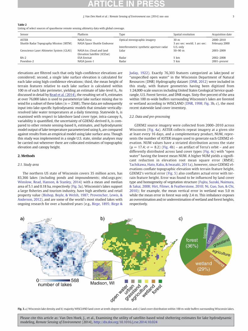
Table 2Listing of select sources of spaceborne remote sensing altimetry data with global coverage.

Sensor Platform Type Spatial resolution Acquisition date

ASTER NASA Terra Optical stereographic imagery 30 m 2000–2010Shuttle Radar Topography Mission (SRTM) NASA Space Shuttle Endeavor

Interferometric synthetic aperture radar3 arc-sec: world; 1 arc-sec:U.S. only

February 2000

Geoscience Laser Altimeter System (GLAS) NASA Ice, Cloud and landElevation Satellite (ICESat)

Lidar 50–90 m 2003–2009

RA-2 ESA Envisat Radar 5 km 2002–2008Poseidon-2 NASA Jason-1 Radar 5 km 2001–present

3J. Van Den Hoek et al. / Remote Sensing of Environment xxx (2014) xxx–xxx

elevations are filtered such that only high-confidence elevations areconsidered; second, a single lake surface elevation is calculated foreach lake using high-confidence elevations; third, the mean height ofterrain features relative to each lake surface is calculated within100 m of each lake perimeter, yielding an estimate of lake-level hs. Asdiscussed in detail by Read et al. (2014), the resulting set of hs estimatesat over 76,000 lakes is used to parameterize lake surface mixing due towind for a subset of these lakes (n=2368). These data are subsequentlyinput into lake-specific hydrodynamic models that simulate vertically-resolved lake water temperatures at a daily timestep. Statewide hs isexamined with respect to lakeshore land cover type, intra-canopy hsvariability is quantified, the uncertainty of GDEM2-derived hs is com-pared to other remote sensing-based hs estimates, and hydrodynamicmodel output of lake temperature parameterized using hs are comparedagainst results from an empirical model using lake surface area. Thoughthis study was implemented in a single U.S. state, similar analyses maybe carried out wherever there are collocated estimates of topographicelevation and canopy height.

2. Methods

2.1. Study area

The northern US state of Wisconsin covers 35 million acres, has83,366 lakes (including ponds and impoundments; nhd.usgs.gov;Winslow, Read, Hanson, & Stanley, 2014) with a mean and medianarea of 5.1 and 0.18 ha, respectively (Fig. 3a). Wisconsin's lakes supporta large fisheries and tourism industry, have high aesthetic and retailproperty value (Bishop, Boyle, & Welsh, 1987; Provencher, Lewis, &Anderson, 2012), and are some of the world's most studied lakes withongoing research for over a hundred years (e.g., Birge, 1895; Birge &

Fig. 3. a)Wisconsin lake density and b)majorityWISCLAND land cover at tenth-degree resoluti

Please cite this article as: Van Den Hoek, J., et al., Examining the utilitymodeling, Remote Sensing of Environment (2014), http://dx.doi.org/10.101

Juday, 1922). Exactly 76,303 features categorized as lake/pond or“unspecified open water” in the Wisconsin Department of NaturalResources (DNR) Hydrography dataset (DNR, 2012) were included inthis study, with feature geometries having been digitized from1:24,000-scale sources including United States Geological Service quad-rangle, U.S. Forest Service, and DNRmaps. Sixty-five percent of the areawithin 100 m-wide buffers surrounding Wisconsin's lakes are forestedor wetland according to WISCLAND (DNR, 1998; Fig. 3b, c), the mostrecent statewide land cover inventory.

2.2. Data and pre-processing

GDEM2 source imagery were collected from 2000–2010 acrossWisconsin (Fig. 4a). ASTER collects repeat imagery at a given siteat least every 16 days, and a complementary product, NUM, repre-sents the number of ASTER images used to generate each GDEM2 el-evation. NUM values have a striated distribution across the state(μ = 17.4; σ = 8.2) (Fig. 4b) – an artifact of Terra's orbit – and aredifferently distributed across land cover types (Fig. 4c) with “openwater” having the lowest mean NUM. A higher NUM yields a signifi-cant reduction in elevation root mean square error (RMSE;Tachikawa, Hato, Kaku, & Iwasaki, 2011a), however, since GDEM2 el-evations conflate topographic elevation with terrain feature height,GDEM2's vertical error (Fig. 5) also conflates actual error with ter-rain feature height. Error was found to be influenced by land covertype and homogeneity of vegetation structure (Fujita, Suzuki, Nuimura,& Sakai, 2008; Hirt, Filmer, & Featherstone, 2010; Ni, Guo, Sun, & Chi,2010); for example, the mean vertical error in wetland was 5.0 mwhile the mean error in forest was only 2.4 m. This imbalance exposesan overestimation and/or underestimation ofwetland and forest heights,respectively.

on, and c) land cover distributionwithin 100m-wide buffers surroundingWisconsin lakes.

of satellite-based wind sheltering estimates for lake hydrodynamic6/j.rse.2014.10.024

Fig. 4. a) GDEM2 elevation and b)NUMvalue distribution acrossWisconsinwith c)mean elevation (filled bars) and NUM (hollowbars) and respective standard deviations forWISCLANDland covers.

4 J. Van Den Hoek et al. / Remote Sensing of Environment xxx (2014) xxx–xxx

Prior to calculating zlake and then hs, GDEM2 elevations were pre-processed in two ways. First, to limit the influence of “mixed pixels”that straddled the lake surface and lakeshore, only pixels with centroidslocated more than 30 m within a lake perimeter were used to estimate

Fig. 5.Mean vertical errors between the GDEM2 and GPS benchmark elevations by 2006National Land Cover Database land cover type (www.mrlc.gov/nlcd06_data.php). Adaptedfrom Tachikawa et al. (2011b).

Please cite this article as: Van Den Hoek, J., et al., Examining the utilitymodeling, Remote Sensing of Environment (2014), http://dx.doi.org/10.101

the lake's surface elevation. Second, pixels were progressively fil-tered by NUM such that only the highest confidence elevation valueswere used to calculate zlake: the percent coverage of pixels withNUM≥ 22, i.e., μopen water + σopen water, was calculated and additionalpixels with progressively lower NUM values were included throughNUM = 6, i.e., μopen water − σopen water, until at least 25% coveragewas achieved. Approximately 9700 (12%) of lakes did not reach ade-quate coverage of high-confidence GDEM2 pixels and were excludedfrom the analysis.

2.3. Analysis

Mean hs was estimated for a given lake in two stages (Fig. 6). First,the lake surface elevation, zlake, was calculated as the mean elevationof high-confidence GDEM2 pixels within a lake perimeter. Second, abuffer was created around each lake perimeter, the width of whichshould be adequate to capture the region of the canopy in the bufferthat shelters the lake. For example, if a lake featured a continuous rowof trees, i.e. wind break, a small buffer on the order of 30mmay suffice.If, on the other hand, hs increased with distance from the lakeshore, awider buffer would be required to encompass the tallest trees in thecanopy. To identify a suitable buffer width, the incremental increase inhs, i.e., the fractional increase in hs relative to the maximum hs recordedwithin a given buffer width, was considered. The incremental increasein hs was measured across buffer widths from 10–200 m at 66 mainlyforested lakes in northern Wisconsin with GDEM2 as well as high-resolution G-LiHT lidar coverage. For both GDEM2 and G-LiHT, the frac-tional increases of hs beyond 100 m were very low — 4% and 2% for

of satellite-based wind sheltering estimates for lake hydrodynamic6/j.rse.2014.10.024

Fig. 6.Methodology for determining the sheltering height, hs, within a given lake buffer.

5J. Van Den Hoek et al. / Remote Sensing of Environment xxx (2014) xxx–xxx

GDEM2 and G-LiHT, respectively. Given the low incremental increase inhs, 100 m was selected for the lake buffer width.

Within each lake's 100m-wide buffer, hswas calculated as themeandifference between the GDEM2 elevation and zlake. In cases where twoor more buffers overlaid a given GDEM2 pixel, themean of the associat-ed zlake values was used as the reference lake surface elevation. Thestatewide distribution of hs was examined with respect to WISCLANDland cover type, within-buffer variability of hs was quantified, andGDEM2 hs values were compared to 90m SRTMV2 DEM- (hereafter re-ferred to as SRTM) and G-LiHT-derived hs, as well as hc values from theSimard et al. (2011) 1 km resolution global forest canopy height map.(Note that despite 30 m resolution SRTM data being available in theU.S., 90 m resolution SRTM data were still considered to support thestudy's relevance outside of the U.S.) Finally, the goodness of fit be-tween modeled and observed lake water temperatures were compared

Please cite this article as: Van Den Hoek, J., et al., Examining the utilitymodeling, Remote Sensing of Environment (2014), http://dx.doi.org/10.101

using GDEM2 and SRTM hs-parameterized wind shear values as well astheHondzo and Stefan (1993) lake surface area-parameterizedmethod.

3. Results and discussion

3.1. Statewide hs distribution

A mean and median hs of 2.1 and 1 m, respectively, were calculatedacross 76,303 Wisconsin lake buffers with greater hs and wind shelter-ing potential measured across the state's northern forests (Fig. 7a).There were typically three land covers within a single buffer with forestcover being dominant in terms of abundance (36% of statewide bufferarea) as well as hs (Fig. 7b). However, since ht and hc cannot be mea-sured independently of hs, differences in hs between land cover types re-sult from intra-buffer topographic variability as well as the variationinherent in the heights of trees, shrubs, grasses, etc. Nonetheless, hsestimated for grassland and agriculture was comparable to “typical” hcvalues from Table 1, while forest hs was 2 and 4 m less than the lowestestimate for woodland trees or coniferous forest hs, respectively.

While median GDEM2 hs in forest-dominated buffers (6m)was rea-sonable, hs was almost certainly overestimated in buffers dominated bywater (4 m) or grassland (5 m). In addition to the issue of overlookingwithin-buffer hs and land cover diversity (discussed in Section 3.2below), there were multiple factors that may have contributed to thisoverestimation. First, a spatial misregistration between WISCLAND,GDEM2, and DNR lake feature geometry is evident in open water pixelsmaking up 9% of total lakeshore buffer area; inclusion of shoreline to-pography in the GDEM2 water mask was also identified by Tachikawa,Kaku, et al. (2011b) as a potential source of error. Second, and related,the omission of small lakes in the GDEM2water mask would have con-tributed to spurious elevationswithin the lake as well as the immediatelakeshore area (Jing, Shortridge, Lin, &Wu, 2014). Third, theremayhavebeen a disconnect between a given location's spectral characteristicsupon which the WISCLAND land cover classification was based andstructural characteristics that drove the GDEM2 elevation measure-ment. This spectral–structural incongruity was evident in the 4 mmedian hs of open water, likely a result of open water dominatingthese pixels' spectral signatureswhile the heights of non-water featuresyielded a non-negligible hs. Fourth, land cover changes that occurredbetween respective imagery collection periods for WISCLAND (1991–1993) and GDEM2 (2000–2010) would have affected respective assess-ments of land cover and elevation.

Approximately 28,500 (37%) lake buffers had a negative hs meaningthat the mean GDEM2 elevation within the buffer was less than that ofthe lake surface. A negative buffer hs could have arisen from an overes-timation of zlake or an underestimation of hs at the pixel-level. Consider-ing the former, GDEM2 zlake values were exceptionally correlated withSRTM-derived zlake values (Fig. 8a; Li et al., 2012). However, SRTM andGDEM2 zlake showed a high RMSE of 6.61 m statewide, and GDEM2tended to overestimate respective SRTM and G-LiHT estimates of zlake(Fig. 8b). In addition to GDEM2's overestimation of zlake identifiedhere, Carabajal (2011), Li et al. (2012), and Suwandana, Kawamura,Sakuno, Kustiyanto, and Raharjo (2012) found systematic underestima-tion of GDEM2 elevations across land covers, and Ni et al. (2010, 2013),Gesch, Oimoen, Zhang, Danielson, and Meyer (2011), and Tachikawa,Kaku, et al. (2011b) each documented GDEM2's underestimation of for-est cover, specifically. Both the overestimation of zlake and the underes-timation of pixel-level hs thus likely contributed to the presence ofnegative buffer hs. Notably, negative buffer hs were also measured at23%of lake buffers using SRTMdata, suggesting that anunderestimationof terrain feature elevations was not solely an issue with GDEM2.

3.2. Within-buffer hs variability

The standard deviation of median hs across Wisconsin's lakes grewfrom 3.6–5.5 m with increasing lake surface area (Fig. 9). Variability in

of satellite-based wind sheltering estimates for lake hydrodynamic6/j.rse.2014.10.024

Fig. 7. Median buffer hs across a) Wisconsin at tenth-degree resolution and b) dominant WISCLAND land covers within 100 m-wide lake buffers.

6 J. Van Den Hoek et al. / Remote Sensing of Environment xxx (2014) xxx–xxx

hs is especially important in small lakes since they are, first, moresensitive to shoreline sheltering and, second, disproportionately in-fluential in carbon cycling (Bastviken, Tranvik, Downing, Crill, &

Fig. 8. Comparison of GDEM2- and SRTM-derived mean lake surface elevations, zlake,across a) Wisconsin lakes with mutual coverage (RMSE 95% CI = 6.53–6.70), andb) lakes with high-resolution G-LiHT lidar coverage (RMSE 95% CI = 5.84–8.31).

Please cite this article as: Van Den Hoek, J., et al., Examining the utilitymodeling, Remote Sensing of Environment (2014), http://dx.doi.org/10.101

Enrich-Prast, 2011; Kortelainen et al., 2006; Post, 2002; Tranviket al., 2009). Within-buffer variability may have resulted from a va-riety of sources such as land cover diversity, patchiness of vegeta-tive cover across buffer terrain, as well as changes in topographicelevation within a buffer. Since a single wind velocity measurementat a representative height above the water surface, i.e. hs, was usedto parameterize momentum flux resulting from wind shear stress(Markfort, Porté-Agel, & Stefan, 2014; Markfort et al., 2010), errorin estimation of wind sheltering may have resulted from within-buffer hs variability. That is, the influence of lake area on hs hadimplications for the selection of a single representative, i.e., mean,hs for a given lake buffer that overlooked potential within-buffervariation in topography and terrain feature height. For lakessurrounded by relatively flat terrain, hs variability was likely negli-gible regardless of size, but on other lakes with prominent vegeta-tion or built-up land cover, small differences on the order of a metercould have had a significant effect on estimated surface shear stress(Markfort et al., 2010). Variability in hs had less of an impact onvery large lakes where wind sheltering was expected to be negligi-ble. However, such large lakesmay experiencemore variation in pre-vailing wind direction across the canopy and lake surface, whichwould influence wind shear stress, though this was not examinedin the present study.

Fig. 9. Violin plots showing the variation of within-buffer hs standard deviation by lakearea quartile. Q1: 0.08 ha; Q2: 0.18 ha; Q3: 0.56 ha; Q4: 8.4 × 106 ha.

of satellite-based wind sheltering estimates for lake hydrodynamic6/j.rse.2014.10.024

Fig. 11. Violin plots comparing the potential biases between GDEM2 hs and SRTM andG-LiHT hs, and Simard hc.

7J. Van Den Hoek et al. / Remote Sensing of Environment xxx (2014) xxx–xxx

3.3. Comparison of hs between remote sensing systems

GDEM2-derived hswere compared to SRTM- (Fig. 10a) and airborneG-LiHT lidar-derived hs (Fig. 10b), as well as hc from the near-global,1 km resolution canopy height map by Simard et al. (2011) (Fig. 10c).For each comparison, a bootstrap procedure was used to calculate the95% confidence interval (CI) for RMSE. Overall, GDEM2 hs were poorlycorrelated with other hs estimates. Of these, GDEM2 showed the bestcorrelation with SRTM (r2 = 0.137; RMSE = 3.88 m) while G-LiHT hsand Simard hc correlate to GDEM2 hs slightly better than a random dis-tribution (r2 = 0.066 and 0.013, respectively). The lack of correlation isnot a surprise given the considerable differences between the data.Periods of imagery acquisition vary meaning that land cover type orcondition may vary between observations, each sensor has a uniquespatial registration (Jing et al., 2014; Miliaresis & Delikaraoglou, 2009;Rawat, Mishra, Sehgal, Ahmed, & Tripathi, 2013; Van Niel, McVicar, Li,Gallant, & Yang, 2008), spatial resolution (Ni et al., 2013), and is differ-ently sensitive to land cover type and condition (Hagberg, Ulander, &Askne, 1995; Sexton, Bax, Siqueira, Swenson, & Hensley, 2009).

Furthermore, elevation products were inferred from remotelysensed data in distinct ways. GDEM2 is a photogrammetric productwhere a given point's elevation is a function of spectral correspondencebetween stereo imagery (Tachikawa, Kaku, et al., 2011b). SRTM is basedon interferometric synthetic aperture radar (InSAR), and a location's el-evation corresponds to the elevation of the radar beam's “scatteringcenter” rather than the “absolute” height of a terrain feature; assuch, SRTM elevations are tightly correlated to vegetation type andcanopy density (Carabajal & Harding, 2006; Kellndorfer et al., 2004;Miliaresis & Delikaraoglou, 2009). Both GDEM2 and SRTM had diffi-culty identifying elevations over stretches of flat terrain such aswater bodies where potential points of correlation and radar back-scatter are reduced (Nikolakopoulos, Kamaratakis, & Chrysoulakis,2006). G-LiHT lidar data (Cook et al., 2013; gliht.gsfc.nasa.gov) had2 m horizontal resolution and 11 mm vertical accuracy, collected multi-ple measurements of vegetation structure from a single pulse— the firstof which corresponded to hc, and offered the most accurate hs measure-ments here, albeit over the smallest extent (75 lakes within an approxi-mately 100 km2 study area). Simard hc is primarily based on spaceborneICESat GLAS lidar data, and corresponds to the tallest return height aboveground (Bolton et al., 2013; Sun, Ranson, Kimes, Blair, & Kovacs, 2008).

Despite GDEM2's overestimation of zlake relative to SRTM (Fig. 8),there was little bias (−0.1 m) between GDEM2 and SRTM hs (Fig. 11).Previous research found similarly correlated errors between GDEM2and SRTM (Amans, Wu, & Ziggah, 2013; Hayakawa, Oguchi, & Lin,2008) suggesting that GDEM2 and SRTM are prone to similar levels ofover- or underestimation. Since SRTM had a coarser resolution (90 m)

Fig. 10. Comparison of GDEM2-derived mean hs with a) SRTM hs (RMSE 95% CI = 3.87–3.94),14.61).

Please cite this article as: Van Den Hoek, J., et al., Examining the utilitymodeling, Remote Sensing of Environment (2014), http://dx.doi.org/10.101

than GDEM2 (30 m), SRTM effectively smoothed the combined topo-graphic and canopy height signal over space, reducing the influence oflocal hs extrema. While GDEM2 and SRTM showed low bias, GDEM2tended to underestimate G-LiHT hs and Simard hc by approximately 7and 13 m, respectively, for distinct reasons. High-resolution G-LiHT hsresponded to fine-scale variation in canopy closure, topographic rise,and, importantly, was not as susceptible to the “mixed pixel” conflationof lake surface and lakeshore terrain elevations in a single measure-ment; this means that G-LiHT wasmore capable of capturing the actual“top of canopy” height rather than the localized average. Simard hc, onthe other hand, only related hc and, therefore, did not incorporate thecontribution of topography, theoretically introducing an underestima-tion of hs. Further, a single Simard 1 km pixel may have covered anentire lake as well as its 100 m buffer meaning that Simard hc data pro-vided a regional estimate of hc rather than one specific to a lake and itsbuffer.

3.4. Hydrologic model output comparison

In order to examine the utility of GDEM2 hs for estimating the windsheltering coefficient (Wst) for lake modeling applications, we com-pared modeled water temperatures with observed temperatures from569 Wisconsin lakes using lake-specific RMSE (°C) as our goodness offit metric. A one-dimensional mechanistic hydrodynamic model, theGeneral LakeModel (GLMv1.2.0),was used for these simulations. Detailsof the modeling approach can be found in Hipsey, Bruce, and Hamilton(2013) or Read et al. (2014), but in brief, GLM is a hydrodynamic

b) G-LiHT lidar hs (RMSE 95% CI = 9.42–12.83), and c) Simard hc (RMSE 95% CI = 14.33–

of satellite-based wind sheltering estimates for lake hydrodynamic6/j.rse.2014.10.024

8 J. Van Den Hoek et al. / Remote Sensing of Environment xxx (2014) xxx–xxx

model that dynamically simulates the vertical distribution of lake watertemperature by accounting for fluxes of mixing energy and heat,e.g., incoming solar radiation. The wind sheltering coefficient used inthe model was parameterized in two ways: first, by using remotesensing-derived (GDEM2 and SRTM) estimates of hs and lake area asinput into the Markfort et al. (2010) model, and, second, by using lakesurface area alone in the empirically-derived lake surface area-to-Wst re-lationship proposed by Hondzo and Stefan (1993). Neither G-LiHT norSimard data were considered since neither offered coverage at morethan three validation lakes. Thus, three different simulation types werecompared that differed only in the value used for each model's windsheltering coefficient; hereafter, we refer to these simulation types ashydroGDEM2, hydroSRTM, and hydroHondzo.

The 569 validation lakes had surface areas between 0.1 to 10 km2

and, being small to medium sized lakes, were expected to be the mostsensitive to wind sheltering (Markfort et al., 2010). Because Hondzoand Stefan's (1993) wind shelteringmodel was calibrated using empir-ical data from forested lakes (these lakes covered the same size rangespecified above), validation lakes were divided into two categories:forest, where the dominant land cover in each lake buffer was forest(n=469), and other, where the dominant land cover in each lake bufferwas urban, agricultural, grassland, wetland, or water (n= 100; Fig. 3c).Simulations spanned 1979 to 2011, and resulting temperature profileswere comparedwith corresponding observational data collected duringthis time period. Temporally-matchedmodeled and observed datawereused to calculate a RMSE value for each lake and for each of the threesimulation types (total of 1707 simulations). Any lakes with an RMSEvalue above 3 °C for all three wind sheltering methods (n = 194)were excluded from our final evaluation, as these poor model fitswere likely due to other biases or errors in the model parameters orinput data. After removing these errant lakes, the RMSEs resultingfrom hydroGDEM2, hydroSRTM, and hydroHondzo were compared usingpaired t-tests.

For forested lakes, there was no statistically significant differencebetween model quality for the three types of wind sheltering used(Fig. 12). For other dominant land cover types, hydroGDEM2 andhydroSRTM were both statistically significant improvements over thesimpler hydroHondzo: hydroGDEM2 resulted in a 0.40 °C RMSE reduction(p=0.015; RMSE 95% CI=0.043–0.767),while hydroSRTM had an aver-age reduction of 0.43 °C RMSE (p = 0.002; RMSE 95% CI = 0.137–0.717). A reduction in RMSE between 0.40 and 0.43 °C may sound

Fig. 12. Comparison of hydrodynamic model RMSE for lakes dominated by forest(n = 315) and urban, agricultural, grassland, wetland, or water land cover (categorizedas “Other”; n= 60).Wind sheltering parameters for lake hydrodynamicmodels were cal-culated using lake surface area and hs (“GDEM2” and “SRTM”) following Markfort et al.(2010), or lake surface area following Hondzo and Stefan (1993; “Hondzo”).

Please cite this article as: Van Den Hoek, J., et al., Examining the utilitymodeling, Remote Sensing of Environment (2014), http://dx.doi.org/10.101

small but represents a decrease in overall modeling error by approxi-mately 15%. There are many additional sources of modeling error thatcannot be improved by refining estimates of sheltering height. For ex-ample, in a study where wind sheltering was used as a free parameterto minimize individual lake RMSE, the typical lake RMSE was stillapproximately 1.4 °C (Fang et al., 2012), which represents an upperlimit of modeling accuracy with perfect wind sheltering estimates.

Non-forested lakes with surface areas between 0.5 to 1.1 km2 hadthe greatest improvement (compared to other size ranges) overHondzo and Stefan (1993)when thewind sheltering coefficientwas pa-rameterized with GDEM2 or SRTM estimates of hs (0.72 °C and 0.68 °Caverage improvement in RMSE, respectively; n=17 lakes). These initialresults provided no evidence to suggest that remote sensing-derived es-timates of hs improved lake models for forested lakes, indicatinghydroHondzo captures most of the important pattern in sheltering acrossnorth temperate forested lakes. But these results indicate that for non-forested lakes, GDEM2 and, especially, SRTM-based hs estimates capturevariability that the Hondzo-based method does not and significantlyimproved lake water temperature simulations as a result. With watertemperature trends around 0.45 °C per decade (Schneider & Hook,2010), the reductions in model error through integrating hs improveour ability to understand, model, and predict lake-specific change andclimate response across large populations of lakes.

3.5. Limitations & future work

The methodology proposed here to use GDEM2 to estimate hs offersmany advantages over current practices as it is readily scalable, hasnear-global coverage, and captures hs at small as well as large lakes.However, GDEM2 source data are limited in that they are effectively acomposite of elevations from stereographic imagery acquired between2000 and 2010, and are therefore not only out-of-date but may beout-of-sync with complementary land cover or observational lake tem-perature data. Future studies should therefore consider using a landcover classification based on imagery that were concomitantly collectedwith GDEM2 source imagery. GDEM2 is further limited by the spatialmisregistration between lake feature geometry data like the DNR(2012) data considered here. Future studies could adopt lake feature ge-ometry that conforms to water bodies depicted in the GDEM2 watermask, or, following Arefi and Reinartz (2011), improve estimates ofzlake by correcting GDEM2 shoreline elevations. With better temporallysynchronized land cover, lake feature geometry, and hs data, the poten-tial influence of land cover change on the lake energy budget could beassessed and, for those lakes with elevation gauges, lake surface eleva-tions could be dynamically updated and incorporated in hs assessments.

A 100 m buffer width was used across all lakes regardless lakeshoretopographic complexity or within-buffer canopy variability. Ideally, thebuffer widthwould respond to both of these factors such that the bufferwould only bewide enough to capture the canopy that immediate shel-ters the lake and nothingmore, thus excluding sites of lower (and irrel-evant) hs. Similarly, each land cover type within a given buffer wouldideally be assigned an indicator of surface roughness as this affects theapproaching turbulent boundary layer (Garratt, 1992).

The model for wind sheltering used in this work assumes that lakescan be approximated as having a nearly round shape with a uniformsheltering height around the lake perimeter. For lakes that do notmeet these criteria, either due to an elongated shape or non-uniform to-pographic or canopy heights along the shoreline, a wind direction-dependent sheltering height may be considered. Alternatively, thewind direction distribution may be employed to determine a winddirection-weighted sheltering coefficient. Moreover, the wind shelter-ing model employed here is specifically designed for one-dimensionallake hydrodynamicmodels (e.g., Read et al., 2014). If variation in surfacewind shear is required for a multi-dimensional model (e.g. Dietrichet al., 2011; Hodges, Imberger, Saggio, & Winters, 2000; Rueda, Vidal,& Schladow, 2009), the variation in surface energy flux with fetch

of satellite-based wind sheltering estimates for lake hydrodynamic6/j.rse.2014.10.024

9J. Van Den Hoek et al. / Remote Sensing of Environment xxx (2014) xxx–xxx

(i.e., the length of water overwhichwind blows), presented inMarkfortet al. (2010) and Markfort et al. (2014), may be employed.

While GDEM2's spatial resolution provides coverage across abreadth of lake and buffer sizes – offering the greatest coverage of anysystem considered here – it is too coarse to capture sub-pixel forest can-opy gaps or local topographic rise thereby precluding examination ofcanopy texture's role on wind shear stress. The ever-expanding cover-age by high-resolution airborne lidar systems like G-LiHT as well assub-meter resolution commercial satellite stereographic imagery(e.g., IKONOS or the upcoming WorldView-3) offers an unprecedentedopportunity to generate canopy heightmodelswith exceptional verticalaccuracy (e.g., Neigh et al., 2014), or fuseGDEM2with high-resolution to-pographic elevation data (Ni et al., 2013). Very high-resolution imagerycould further be used to map lake feature geometry at improved spatialdetail (e.g., Sawaya, Olmanson, Heinert, Brezonik, & Bauer, 2003).

4. Conclusion

Much work has been done to parameterize wind-driven surface dy-namics on individual lakes for which in-situ observations are available,but efforts to estimate temperature andmixing dynamics for large pop-ulations of lakes that would facilitate process-based estimates are large-ly nonexistent. The methodology proposed here offers a template for aremote sensing-based estimate of sheltering height, hs, needed for esti-matingwind shear stress on lakes, which is a critical boundary conditionfor understanding andmodeling lake processes. Thirtymeter resolutionASTERGDEM2 datawere used to estimate hswithin 100m-wide bufferssurrounding 76,303 Wisconsin lakes, and a hydrodynamic modelparameterized using these hs was applied across 375 lakes. GDEM2hs were shown to improve modeled lake temperature RMSE in non-forested lakes by 0.72 °C, a marked improvement over standardmethods to estimate lake-level wind sheltering at non-forested lakes.This study is valuable not only because of the improvement to modeledlake temperatures it provided, but also for its support of interdisciplin-ary collaboration between terrestrial remote sensing and limnologicalcommunities to address a problem central to understanding the func-tion of lakes in globally relevant processes, including carbon cycling.

Acknowledgments

This research was supported by an appointment to the NASA Post-doctoral Program at the Goddard Space Flight Center, administered byOak Ridge Associated Universities through a contract with NASA.Additional support provided by the U.S. Geological Survey Center forIntegrated Data Analytics, the Wisconsin Department of Natural Re-sources Federal Aid in Sport Fish Restoration (Project F-95-P) and theNational Science Foundation (DEB-0941510). ASTER GDEM2 is a prod-uct ofMETI andNASA. Anyuse of trade,firm, or product names is for de-scriptive purposes only and does not imply endorsement by the U.S.Government.

References

Amans, O.C., Wu, B., & Ziggah, Y.Y. (2013). Assessing vertical accuracy of SRTM Ver 4.1 andASTER GDEM Ver 2 using differential GPS measurements—Case study in Ondo StateNigeria. International Journal of Scientific and Engineering Research, 4(12), 523–531.

Arefi, H., & Reinartz, P. (2011). Accuracy enhancement of ASTER global digital elevationmodels using ICESat data. Remote Sensing, 3(7).

Bastviken, D., Tranvik, L.J., Downing, J.A., Crill, P.M., & Enrich-Prast, A. (2011). Freshwatermethane emissions offset the continental carbon sink. Science, 331(6013), 50. http://dx.doi.org/10.1126/science.1196808.

Birge, E.A. (1895). Plankton studies on Lake MendotaVol. 10.Birge, E.A., & Juday, C. (1922). The inland lakes of Wisconsin: the dissolved gases of the water

and their biological significance. Vol. 64, (The State).Bishop, R.C., Boyle, K.J., & Welsh, M.P. (1987). Toward total economic valuation of Great

Lakes fishery resources. Transactions of the American Fisheries Society, 116(3),339–345.

Bolton, D.K., Coops, N.C., & Wulder, M.A. (2013). Investigating the agreement betweenglobal canopy height maps and airborne Lidar derived height estimates overCanada. Canadian Journal of Remote Sensing, 39(s1), S139–S151.

Please cite this article as: Van Den Hoek, J., et al., Examining the utilitymodeling, Remote Sensing of Environment (2014), http://dx.doi.org/10.101

Carabajal, C.C. (2011). ASTER global DEM version 2.0 evaluation using ICESat geodeticground control. http://www.jspacesystems.or.jp/ersdac/GDEM/ver2Validation/Appendix_D_ICESat_GDEM2_validation_report.pdf Available at

Carabajal, C.C., & Harding, D.J. (2006). SRTM C-band and ICESat laser altimetry elevationcomparisons as a function of tree cover and relief. Photogrammetric Engineering andRemote Sensing, 72(3), 287–298.

Cole, J.J., Prairie, Y.T., Caraco, N.F., McDowell, W.H., Tranvik, L.J., Striegl, R.G., et al. (2007).Plumbing the global carbon cycle: integrating inland waters into the terrestrial car-bon budget. Ecosystems, 10(1), 172–185.

Cook, B., Corp, L., Nelson, R., Middleton, E., Morton, D., McCorkel, J., et al. (2013). NASAGoddard's LiDAR, Hyperspectral and Thermal (G-LiHT) airborne imager. RemoteSensing, 5(8), 4045–4066. http://dx.doi.org/10.3390/rs5084045.

Dietrich, J.C., Zijlema, M., Westerink, J.J., Holthuijsen, L.H., Dawson, C., Luettich, R.A., Jr.,et al. (2011). Modeling hurricane waves and storm surge using integrally-coupled,scalable computations. Coastal Engineering, 58(1), 45–65.

DNR (2012). Surface water (hydrography) data. http://dnr.wi.gov/maps/gis/datahydro.html (Retrieved from)

DNR (Department of Natural Resources) (1998). WISCLAND land cover. http://dnr.wi.gov/maps/gis/datalandcover.html (Retrieved from)

Downing, J.A. (2010). Emerging global role of small lakes and ponds: Little things mean alot. Limnetica, 1(29), 9–24 Retrieved from http://revistes.iec.cat/index.php/limnetica/article/view/39973.

Downing, J.A., Cole, J.J., Middelburg, J.J., Striegl, R.G., Duarte, C.M., Kortelainen, P., et al.(2008). Sediment organic carbon burial in agriculturally eutrophic impoundmentsover the last century. Global Biogeochemical Cycles, 22(1).

Fang, X., Alam, S.R., Stefan, H.G., Jiang, J., Jacobson, P.C., & Pereira, D.L. (2012). Simulationsof water quality and oxythermal cisco habitat in Minnesota lakes under past and fu-ture climate scenarios. Water Quality Research Journal of Canada, 47(3–4), 375–388.http://dx.doi.org/10.2166/wqrjc.2012.031.

Farr, T.G., Rosen, P.A., Caro, E., Crippen, R., Duren, R., Hensley, S., et al. (2007). The shuttleradar topography mission. Reviews of geophysics, 45(2).

Fujita, K., Suzuki, R., Nuimura, T., & Sakai, A. (2008). Performance of ASTER and SRTMDEMs, and their potential for assessing glacial lakes in the Lunana region, BhutanHimalaya. Journal of Glaciology, 54(185), 220–228.

Garratt, J.R. (1992). The atmospheric boundary layer. New York: Cambridge UniversityPress.

Gesch, D., Oimoen, M., Greenlee, S., Nelson, C., Steuck, M., & Tyler, D. (2002). The na-tional elevation dataset. Photogrammetric Engineering and Remote Sensing, 68(1),5–11.

Gesch, D., Oimoen, M., Zhang, Z., Danielson, J., & Meyer, D. (2011). Validation of the ASTERGlobal Digital Elevation Model (GDEM) version 2 over the conterminous UnitedStates. http://www.jspacesystems.or.jp/ersdac/GDEM/ver2Validation/Appendix_B_CONUS%20_GDEMv2_validation_report.pdf (Available at)

Hagberg, J.O., Ulander, L.M.H., & Askne, J. (1995). Repeat-pass SAR interferometry overforested terrain. IEEE Transactions on Geoscience and Remote Sensing, 33(2),331–340. http://dx.doi.org/10.1109/36.377933.

Hanson, P.C., Carpenter, S.R., Cardille, J.A., Coe, M.T., & Winslow, L.A. (2007). Small lakesdominate a random sample of regional lake characteristics. Freshwater Biology,52(5), 814–822. http://dx.doi.org/10.1111/j.1365-2427.2007.01730.x.

Hayakawa, Y.S., Oguchi, T., & Lin, Z. (2008). Comparison of new and existing globaldigital elevation models: ASTER G‐DEM and SRTM‐3. Geophysical Research Letters,35(17).

Hipsey, M.R., Bruce, L.C., & Hamilton, D.P. (2013). GLM General Lake Model. Modeloverview and user information. Perth, Australia: The University of WesternAustralia.

Hirt, C., Filmer, M.S., & Featherstone, W.E. (2010). Comparison and validation of therecent freely available ASTER-GDEM ver1, SRTM ver4. 1 and GEODATA DEM-9Sver3 digital elevation models over Australia. Australian Journal of Earth Sciences,57(3), 337–347.

Hodges, B.R., Imberger, J., Saggio, A., &Winters, K.B. (2000). Modeling basin-scale internalwaves in a stratified lake. Limnology and Oceanography, 45(7), 1603–1620.

Hondzo, M., & Stefan, H.G. (1993). Regional water temperature characteristics of lakessubjected to climate change. Climatic Change, 24(3), 187–211. http://dx.doi.org/10.1007/BF01091829.

Jing, C., Shortridge, A., Lin, S., & Wu, J. (2014). Comparison and validation of SRTM andASTER GDEM for a subtropical landscape in Southeastern China. InternationalJournal of Digital Earth, 12(7), 1–24.

Kankaala, P., Huotari, J., Tulonen, T., & Ojala, A. (2013). Lake-size dependent physical forc-ing drives carbon dioxide and methane effluxes from lakes in a boreal landscape.Limnology and Oceanography, 58, 1915–1930.

Kellndorfer, J.M., Walker, W.S., Pierce, L., Dobson, C., Fites, J.A., Hunsaker, C., et al. (2004).Vegetation height estimation from Shuttle Radar Topography Mission and NationalElevation Datasets. Remote Sensing of Environment, 93(3), 339–358. http://dx.doi.org/10.1016/j.rse.2004.07.017.

Kortelainen, P., Rantakari, M., Huttunen, J.T., Mattsson, T., Alm, J., Juutinen, S., et al. (2006).Sediment respiration and lake trophic state are important predictors of large CO2 eva-sion from small boreal lakes. Global Change Biology, 12(8), 1554–1567. http://dx.doi.org/10.1111/j.1365-2486.2006.01167.x.

Kouraev, A.V., Semovski, S.V., Shimaraev, M.N., Mognard, N.M., Légresy, B., & Remy, F.(2007). Observations of Lake Baikal ice from satellite altimetry and radiometry.Remote Sensing of Environment, 108(3), 240–253.

Lefsky, M.A. (2010). A global forest canopy height map from the Moderate Resolution Im-aging Spectroradiometer and the Geoscience Laser Altimeter System. GeophysicalResearch Letters, 37(15). http://dx.doi.org/10.1029/2010GL043622 (n/a–n/a).

Li, P., Shi, C., Li, Z., Muller, J. -P., Drummond, J., Li, X., et al. (2012). Evaluation of ASTERGDEM ver2 using GPS measurements and SRTM ver4.1 in China. XXII Congress of

of satellite-based wind sheltering estimates for lake hydrodynamic6/j.rse.2014.10.024

10 J. Van Den Hoek et al. / Remote Sensing of Environment xxx (2014) xxx–xxx

International Society of Photogrammetry. Remote Sensing and Spatial InformationSciences. (pp. 181–186) (Retrieved from http://eprints.gla.ac.uk/64163/).

Markfort, C.D., Perez, A.L., Thill, J.W., Jaster, D.A., Porté-Agel, F., & Stefan, H.G. (2010).Windsheltering of a lake by a tree canopy or bluff topography. Water Resources Research,46(3).

Markfort, C.D., Porté-Agel, F., & Stefan, H.G. (2014). Canopy-wake dynamics and windsheltering effects on Earth surface fluxes. Environmental Fluid Mechanics, 14(3),663–697. http://dx.doi.org/10.1007/s10652-013-9313-4.

McDonald, C.P., Stets, E.G., Striegl, R.G., & Butman, D. (2013). Inorganic carbon loading as aprimary driver of dissolved carbon dioxide concentrations in the lakes and reservoirsof the contiguous United States. Global Biogeochemical Cycles, 27(2), 285–295.

Medina, C.E., Gomez-Enri, J., Alonso, J.J., & Villares, P. (2008). Water level fluctuations de-rived from ENVISAT Radar Altimeter (RA-2) and in-situ measurements in a subtrop-ical water body: Lake Izabal (Guatemala). Remote Sensing of Environment, 112(9),3604–3617.

Miliaresis, G., & Delikaraoglou, D. (2009). Effects of percent tree canopy density and DEMmisregistration on SRTM/NED vegetation height estimates. Remote Sensing, 1(2),36–49.

Neigh, C.S.R., Masek, J.G., Bourget, P., Cook, B., Huang, C., Rishmawi, K., et al. (2014).Deciphering the precision of stereo IKONOS canopy height models for US forestswith G-LiHT airborne LiDAR. Remote Sensing, 6(3), 1762–1782.

Ni, W., Guo, Z., Sun, G., & Chi, H. (2010). Investigation of forest height retrieval usingSRTM-DEM and ASTER-GDEM. IEEE, 2111–2114. http://dx.doi.org/10.1109/IGARSS.2010.5651443.

Ni,W., Sun, G., & Ranson, K.J. (2013). Characterization of ASTER GDEM elevation data overvegetated area compared with lidar data. International Journal of Digital Earth. http://dx.doi.org/10.1080/17538947.2013.861025 (1–14).

Nikolakopoulos, K.G., Kamaratakis, E.K., & Chrysoulakis, N. (2006). SRTM vs ASTER eleva-tion products. Comparison for two regions in Crete, Greece. International Journal ofRemote Sensing, 27(21).

Oke, T.R. (1987). Boundary layer climates (2nd ed.). New York: Routledge.Post, D. (2002). Using stable isotopes to estimate trophic position: Models, methods, and

assumptions. Ecology, 83(3), 703–718. http://dx.doi.org/10.2307/3071875.Provencher, B., Lewis, D.J., & Anderson, K. (2012). Disentangling preferences and expecta-

tions in stated preference analysis with respondent uncertainty: The case of invasivespecies prevention. Journal of Environmental Economics and Management, 64(2),169–182. http://dx.doi.org/10.1016/j.jeem.2012.04.002.

Rawat, K.S., Mishra, A.K., Sehgal, V.K., Ahmed, N., & Tripathi, V.K. (2013). Comparativeevaluation of horizontal accuracy of elevations of selected ground control pointsfrom ASTER and SRTM DEM with respect to CARTOSAT-1 DEM: A case study ofShahjahanpur district, Uttar Pradesh, India. Geocarto International, 28(5), 439–452.

Raymond, P.A., Hartmann, J., Lauerwald, R., Sobek, S., McDonald, C., Hoover, M., et al.(2013). Global carbon dioxide emissions from inland waters. Nature, 503(7476),355–359. http://dx.doi.org/10.1038/nature12760.

Read, J.S., Hamilton, D.P., Desai, A.R., Rose, K.C., MacIntyre, S., Lenters, J.D., et al. (2012).Lake-size dependency of wind shear and convection as controls on gas exchange.Geophysical Research Letters, 39(9). http://dx.doi.org/10.1029/2012GL051886.

Read, J.S., Winslow, L.A., Hansen, G.J.A., Van Den Hoek, J., Hanson, P.C., Bruce, L.C., et al.(2014). Simulating 2368 temperate lakes reveals weak coherence in stratificationphenology. EcologicalModelling, 291, 142–150. http://dx.doi.org/10.1016/j.ecolmodel.2014.07.029.

Roehm, C.L., Prairie, Y.T., & Del Giorgio, P.A. (2009). The pCO2 dynamics in lakes in the bo-real region of northern Québec, Canada. Global Biogeochemical Cycles, 23(3).

Rueda, F., Vidal, J., & Schladow, G. (2009). Modeling the effect of size reduction on thestratification of a large wind‐driven lake using an uncertainty-based approach.Water Resources Research, 45(3).

Please cite this article as: Van Den Hoek, J., et al., Examining the utilitymodeling, Remote Sensing of Environment (2014), http://dx.doi.org/10.101

Sawaya, K.E., Olmanson, L.G., Heinert, N.J., Brezonik, P.L., & Bauer, M.E. (2003). Extendingsatellite remote sensing to local scales: Land and water resource monitoring usinghigh-resolution imagery. Remote Sensing of Environment, 88(1), 144–156.

Schneider, P., & Hook, S.J. (2010). Space observations of inland water bodies show rapidsurface warming since 1985. Geophysical Research Letters, 37. http://dx.doi.org/10.1029/2010GL045059.

Sexton, J.O., Bax, T., Siqueira, P., Swenson, J.J., & Hensley, S. (2009). A comparison of lidar,radar, and field measurements of canopy height in pine and hardwood forests ofsoutheastern North America. Forest Ecology and Management, 257(3), 1136–1147.http://dx.doi.org/10.1016/j.foreco.2008.11.022.

Simard, M., Pinto, N., Fisher, J.B., & Baccini, A. (2011). Mapping forest canopy height glob-ally with spaceborne lidar. Journal of Geophysical Research, 116(G4). http://dx.doi.org/10.1029/2011JG001708.

Slater, J.A., Garvey, G., Johnston, C., Haase, J., Heady, B., Kroenung, G., et al. (2006). TheSRTM data finishing process and products. Photogrammetric Engineering and RemoteSensing, 72(3), 237–247.

Sun, G., Ranson, K.J., Kimes, D.S., Blair, J.B., & Kovacs, K. (2008). Forest vertical structurefrom GLAS: An evaluation using LVIS and SRTM data. Remote Sensing ofEnvironment, 112(1), 107–117.

Suwandana, E., Kawamura, K., Sakuno, Y., Kustiyanto, E., & Raharjo, B. (2012). Evaluationof ASTER GDEM2 in Comparison with GDEM1, SRTM DEM and topographic-map-derived DEM using inundation area analysis and RTK-dGPS data. RemoteSensing, 4(12), 2419–2431. http://dx.doi.org/10.3390/rs4082419.

Swenson, S., & Wahr, J. (2009). Monitoring the water balance of Lake Victoria, East Africa,from space. Journal of Hydrology, 370(1), 163–176.

Tachikawa, T., Hato, M., Kaku, M., & Iwasaki, A. (2011). Characteristics of ASTER GDEMversion 2. Geoscience and Remote Sensing Symposium (IGARSS), 2011 IEEE International(pp. 3657–3660) (IEEE).

Tachikawa, T., Kaku, M., Iwasaki, A., Gesch, D., Oimoen, M., Zhang, Z., et al. (2011). ASTERGlobal Digital Elevation Model Version 2—Summary of Validation Results. www.jspacesystems.or.jp/ersdac/GDEM/ver2Validation/Summary_GDEM2_validation_report_final.pdf (Retrieved from)

Toutin, T. (2008). ASTER DEMs for geomatic and geoscientific applications: A review.International Journal of Remote Sensing, 29(7), 1855–1875.

Tranvik, L.J., Downing, J.A., Cotner, J.B., Loiselle, S.A., Striegl, R.G., Ballatore, T.J., et al.(2009). Lakes and reservoirs as regulators of carbon cycling and climate. Limnologyand Oceanography, 54, 2298–2314.

Van Niel, T.G., McVicar, T.R., Li, L., Gallant, J.C., & Yang, Q. (2008). The impact of misregis-tration on SRTM and DEM image differences. Remote Sensing of Environment, 112(5),2430–2442. http://dx.doi.org/10.1016/j.rse.2007.11.003.

Wang, X., Cheng, X., Gong, P., Huang, H., Li, Z., & Li, X. (2011). Earth science applications ofICESat/GLAS: A review. International Journal of Remote Sensing, 32(23), 8837–8864.http://dx.doi.org/10.1080/01431161.2010.547533.

Winslow, L.A., Read, J.S., Hanson, P.C., & Stanley, E.H. (2014). Lake shoreline in the contig-uous United States: Quantity, distribution and sensitivity to observation resolution.Freshwater Biology, 59(2), 213–223. http://dx.doi.org/10.1111/fwb.12258.

Wulder, M.A., White, J.C., Nelson, R.F., Næsset, E., Ørka, H.O., Coops, N.C., et al. (2012).Lidar sampling for large-area forest characterization: A review. Remote Sensing ofEnvironment, 121, 196–209. http://dx.doi.org/10.1016/j.rse.2012.02.001.

Yamaguchi, Y., Kahle, A.B., Tsu, H., Kawakami, T., & Pniel, M. (1998). Overview of ad-vanced spaceborne thermal emission and reflection radiometer (ASTER). Geoscienceand Remote Sensing, IEEE Transactions on, 36(4), 1062–1071.

Zappa, C.J., McGillis, W.R., Raymond, P.A., Edson, J.B., Hintsa, E.J., Zemmelink, H.J., et al.(2007). Environmental turbulent mixing controls on air–water gas exchange in ma-rine and aquatic systems. Geophysical Research Letters, 34(10).

of satellite-based wind sheltering estimates for lake hydrodynamic6/j.rse.2014.10.024