Embed Size (px)
Citation preview
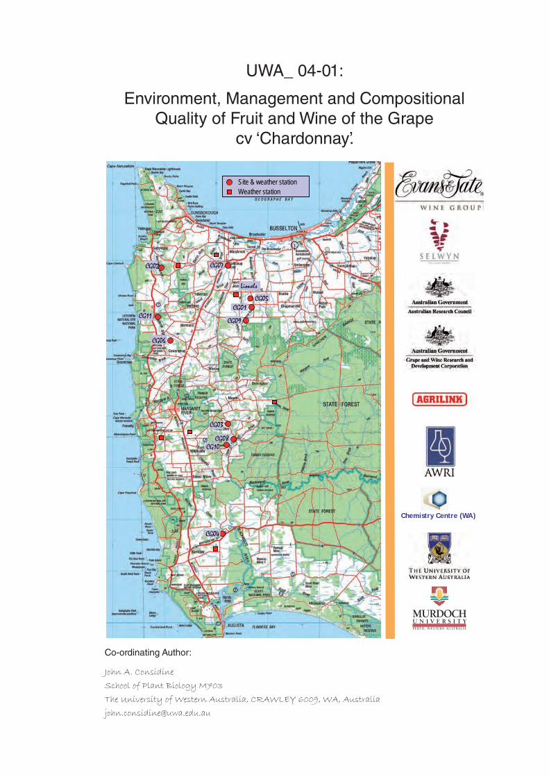
UWA_ 04-01:
Environment, Management and Compositional Quality of Fruit and Wine of the Grape
cv ‘Chardonnay’.
Co-ordinating Author:
John A. Considine
School of Plant Biology M703
The University of Western Australia, CRAWLEY 6009, WA, Australia
Chemistry Centre (WA)
7
Site & weather station
Lionels
CG10CG08
CG03
CG04
CG06
CG11CG09
CG01CG05
CG02 CG07
Weather station
ii
Participant List & Acknowledgements
Environment, Management and Compositional Quality of Chardonnay, cv Gingin.
An Industry – University – Government of Australian Linkage Project
Lead Industry Partner: Evans & Tate Wines/Selwyn Viticultural Services
Supporting Industry Partners: AgriLink International
Chemistry Centre WA
AusCap [informal]
Specterra [via Selwyn Viticultural Services]
Research Agencies:Lead University: The University of Western Australia [Schools, Plant Biology; Biomedical and Chemi-cal Sciences, Computer Science & Software Engineering, Mathematics & Statistics]
Supporting University: Murdoch University [Environmental Science]
Lead Funding Agency: Australian Research Council
Supporting Funding Agency: Grape & Wine R&D Corporation
Supporting Research Agencies:
Australian Wine Research Institute
iVEC (Interactive Virtual Environment Centre, access to super-computing facilities)
Staffing
Contractors:
Department of Agriculture (WA) – Experimental scale wine making
Baigent GeoSciences P/L [Ground Penetrating Radar, Radiometric & electromagnetic map-ping]
Chris Shedley Consulting (Soil Survey)
Farm Link (Craig Neild , Weather Station Maintenance)
Participating Staff
Evans & Tate Wines: Steve Warne, Richard Rowe, Murray Edmonds
Selwyn Viticultural Services: Tom Wisdom
Australian Wine Research Institute: Dr Leigh Francis
Murdoch University: Tom Lyons
University of Western Australia: John Considine (PB), David Glance (CSSE), Kaipillil Vijayan (MS), Emilio Ghisalberti (BCS)
iii
Project Staff:
Tony Robinson (FT, winemaker - project manager), Hazlett Growns (PT, chemistry)
Dr Gabby Pracilio (GIS)
Volunteer: Mr Felipe Burgos (GIS)
Postgraduate students
Joanne Bennett (viticulture),
BSc Hons & BSc Vit & Oenol Project students
AL Robinson, J. Wisdom (Nee Bennett), A. Clarke, S. Pearce, L. Hipper, M. Wood, C. Gazey, K. Maley, A. Isaac
Participating VineyardsClearwater Estate, Jindong, Bridgelands, Carbanup Estate, Alexanders Vineyard, Woodlands Estate, Halcyon, Georgettes, Brockman Estate, Redbrook Estate, Stellar Ridge Estate
AcknowledgementsI wish to thank those industry and partner staff who enabled this project to proceed. In particular Steve Warne, formerly Group Winemaker, Evans & Tate Wines for his initiative, support and enthusiasm for the project from the first concept. To Tom Wisdom and Murray Edmonds who provided essential practical knowledge and guidance and the individual vineyard managers who took time from their busy schedules to assist and guide: Chris Gilmore, Grieg Fowler, Rob Randall, Andrew Field, Andy Ferrara, and Randall Black I also wish to thank the vineyard owners who enabled access and general support: Peter Woods, Mike Calneggia, Graham Connell and Colin Hellier. I also wish to thank Joanne Wisdom for her interest and support, especially during the founding phases of the project and for her work in formalising the protocols.
Staff of AgriLink International provided access to their radio linked weather station network for down-loading data, archiving of data and internet access to data and to their web-based analysis and graph-ing tools.
I also thank staff of the WA Chemistry Centre, Dr Neil Rothnie, Dr Shao Fang Wang, David Harris and Tom Naumovski for their input during the early phases of the project.
I am especially grateful for the input made by the contractors who far exceeded their brief. Andrew Malcolm and Frank Honey (SpecTerra Services P/L); Mark Baigent and Judy Doedens (Baigent Geo-Sciences P/L) and Cr Chris Shedley (Shedley Consulting Services). Their on-going support has been vital and expert.
Finally I wish to thank Tony Robinson for the effort he put in and which was well in excess of normal working hours in an attempt to bring all to fruition. The winemaking was a task to test the most sea-soned winemaker and if problems occurred, they were despite long hours, diligence and dedication to the task. I also wish to thank the many students who worked on short term projects, gathering data which contributed substantially to the unrivalled data sets developed throughout the course of this project.
UWA 04/01 Chardonnay and environment…
page1/2
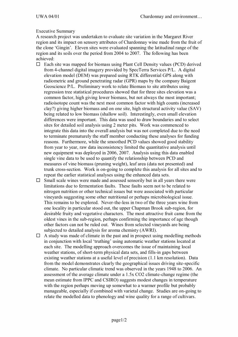
Executive Summary A research project was undertaken to evaluate site variation in the Margaret River region and its impact on sensory attributes of Chardonnay wine made from the fruit of the clone ‘Gingin’. Eleven sites were evaluated spanning the latitudinal range of the region and its soils over the period from 2004 to 2007. The following has been achieved: Each site was mapped for biomass using Plant Cell Density values (PCD) derived
from 4-channel digital imagery provided by SpecTerra Services P/L. A digital elevation model (DEM) was prepared using RTK differential GPS along with radiometric and ground penetrating radar (GPR) maps by the company Baigent Geoscience P/L. Preliminary work to relate Biomass to site attributes using regression tree statistical procedures showed that for three sites elevation was a common factor, high giving lower biomass, but not always the most important; radioisotope count was the next most common factor with high counts (increased clay?) giving higher biomass and on one site, high structural activity value (SAV) being related to low biomass (shallow soil). Interestingly, even small elevation differences were important. This data was used to draw boundaries and to select sites for detailed soil analysis using 2 meter pits. Work was commenced to integrate this data into the overall analysis but was not completed due to the need to terminate prematurely the staff member conducting these analyses for funding reasons. Furthermore, while the smoothed PCD values showed good stability from year to year, raw data inconsistency limited the quantitative analysis until new equipment was deployed in 2006, 2007. Analysis using this data enabled single vine data to be used to quantify the relationship between PCD and measures of vine biomass (pruning weight), leaf area (data not presented) and trunk cross-section. Work is on-going to complete this analysis for all sites and to repeat the earlier statistical analyses using the enhanced data sets.
Small scale wines were made and assessed sensorily but in all years there were limitations due to fermentation faults. These faults seem not to be related to nitrogen nutrition or other technical issues but were associated with particular vineyards suggesting some other nutritional or perhaps microbiological issue. This remains to be explored. Never-the-less in two of the three years wine from one locality in particular stood out, the upper Chapman Brook sub-region, for desirable fruity and vegetative characters. The most attractive fruit came from the oldest vines in the sub-region, perhaps confirming the importance of age though other factors can not be ruled out. Wines from selected vineyards are being subjected to detailed analysis for aroma chemisty (AWRI).
A study was made of climate in the past and in prospect using modelling methods in conjunction with local ‘truthing’ using automatic weather stations located at each site. The modelling approach overcomes the issue of maintaining local weather stations, of short-term physical data sets, and fills-in gaps between existing weather stations at a useful level of precision (1.1 km resolution). Data from the model demonstrates clearly the geographical issues driving site-specific climate. No particular climatic trend was observed in the years 1948 to 2006. An assessment of the average climate under a 1.5x CO2 climate-change regime (the mean estimate from IPPC and CSIRO) suggests modest changes in temperature with the region perhaps moving up somewhat to a warmer profile but probably manageable, especially if combined with varietal change. Studies are on-going to relate the modelled data to phenology and wine quality for a range of cultivars.
UWA 04/01 Chardonnay and environment…
page2/2
1 PhD (being written) and 6 undergraduate ‘honours’ projects were supported by the programme. Two of these studies demonstrated new approaches to the understanding of ‘sluggish’ ferments with cell genetic machinery changes being altered dramatically in the early stages of the log phase and well before a winemaker would detect the occurrence of a defective ferment. This together with the site-specific analysis suggest that further research on fermentation biology may yield benefits for industry.
Recommendations: The project has clearly identified issues for further research, some of which is being undertaken in the on-going evaluation of the data.
1. There appears to be a strong influence of location (management?) on fermentation performance which is not related to nitrogen nutrition or technical aspects of the fermentation as we practiced it.
2. A new approach to ‘ground-truthing’ remotely sensed biomass has been proposed. Evaluation of this is on-going but should provide a method for relating individual vine biomass to remotely sensed imagery values (PCD or soil and land form).
3. Three site factors were shown to be well related to vine biomass for three of the sites: elevation (-ve); radiometric count (+ve) and depth to hardpan (SAV) (+ve). Work is on-going to complete these analyses for the remaining sites.
4. Trunk diameter is proposed as a simple system for estimating vine biomass variation within particular sites. Cane cross section also provides a useful, non-destructive way of estimating leaf area though pruning weight may also be used though this measure is more site specific. It is likely that both measures will need independent calibration for particular cultivars.
5. The modelling approach developed for mapping climate is being applied to other regions within WA and prospectively could be a useful tool for all regions, minimising the need for individual weather stations. The techniques has been used to model climate for Margaret River under a climate change regime and work is in progress to model the prospective impact on vine phenology and wine quality.
6. In the years of vine-monitoring there was evidence of a general increase in vine biomass and for rigid vine management, rather than adaptive management leading to vines pruned sub-optimally and to reduced functional fertility. Improved training for farm hands could lead to more optimal pruning that takes account of within block variation and to higher levels of flower initiation which in a few instances was seriously low. In no instance was the average flower initiation at optimal levels though it was close to that in some vineyards.
John A Considine 20/04/2008
v
Contents
Site characteristics: A. Soil Geoscience 1
Introduction 1Terminology 1
Materials & Methods 1Ground Penetrating Radar 2Data Processing 5GPR Data Products 5Radiometric Data Products 6
Results & Observations 6Radiometric classifications 6
Appendix A: Ground Penetrating Radar Principles 22
Appendix B: Survey Area Maps 23
Soil Surveys of Chardonnay Blocks 25
Introduction 25
Approach 25
Results and Data 25Vineyard CG01 25
Preliminary analyses of spatial data for three sites 63
Preamble 63
Preliminary exploration of relationships between site and vine biomass. 64Observations 64Conclusions 71
CG01: Investigations of the whole block. 72Observations 72Conclusions} 72
Acknowledgements 75
Bibliography 75
Ground-truthing Site CG01 77
Introduction 77
Results & Discussion 80Estimates of vine Biomass 80Attributes, correlation & regression among observations 83
Conclusions 92
vi
Modelling Meso-Climate in Margaret River: the Past and the Prospects under a 1.5x CO2 sce-nario‡. 93
Introduction 93
The Problem 93
The Method 94
The Results 94
Conclusions 95
ACKNOWLEDGEMENTS 96
Bibliography & Further Reading 96
Wine 105
Introduction 105
Materials & Methods 105Chemistry 105Winemaking 107Sensory Analysis 110
Observations and Results 115Sensory attributes: 2004 vintage 115Formal Sensory 2005 vintage 118
Conclusion 123
References 123
Appendix XA-1. 125
The Vineyards and Their Characteristics 127
Introduction 127
Materials and Methods 127
Observations 129
Conclusions 138
APPENDIX 1: Operating Procedures. 145
APPENDIX 2: Non-destructive estimation of leaf area. 150
Method: 150
Analysis and Results 150
Theses Completed or in progress that were sup-ported by this project: 163
PhD 163
Fourth Year Projects 163
vii
List of Figures
Figure 1a-1. GPR antenna behind 4WD 3
Figure 1a-2. Digital acquisition system hardware rack 3
Figure 1A-3. Acquisition laptop and GPS display (on left). 3
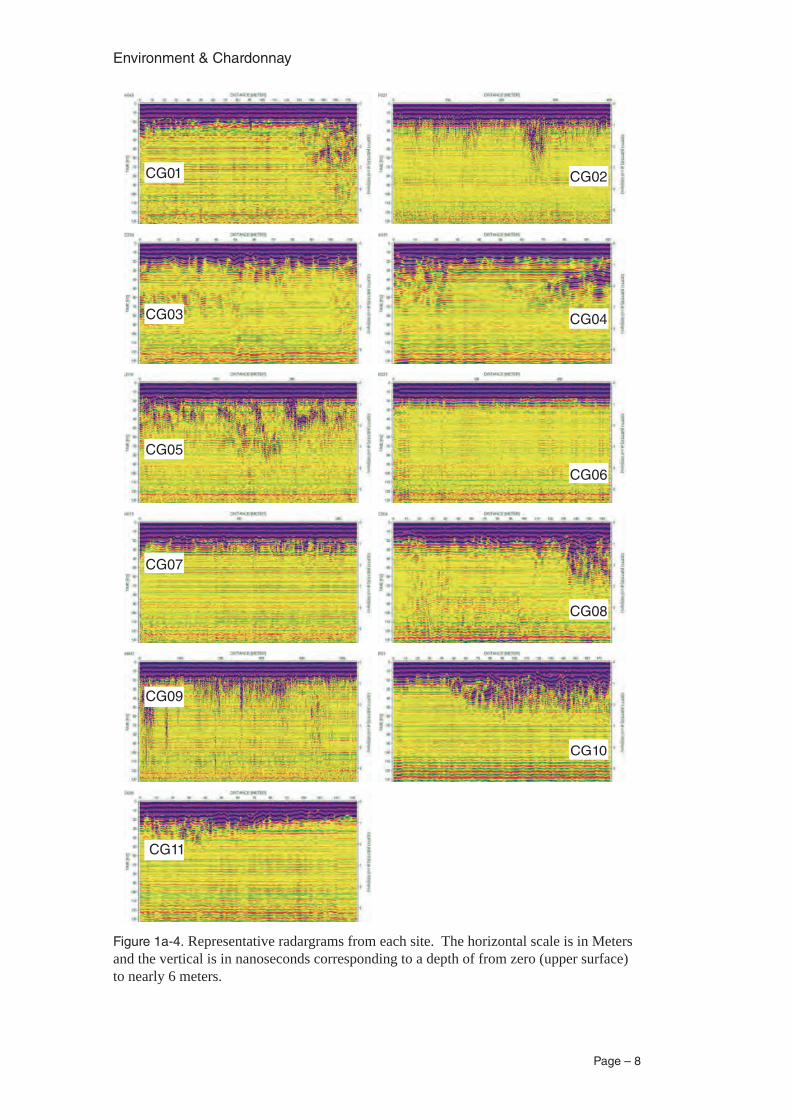
Figure 1a-4. Representative radargrams from each site. The horizontal scale is in Meters and the vertical is in nanoseconds corresponding to a depth of from zero (upper sur-face) to nearly 6 meters. 8
Figure 1a-4. Images for site CG01. 11
Figure 1a-5. Images for site CG02 12
Figure 1a-6. Images for site CG03. 13
Figure 1a-7. Images for site CG04. 14
Figure 1a-8. Images for site CG05. 15
Figure 1a-90. Images for site CG06. 16
Figure 1a-10. Images for site CG07. 17
Figure 1a-11. Images for site CG08. 18
Figure 1a-12. Images for site CG09. 19
Figure 1a-13. Images for site CG10. 21
Figure 1A-14. Images for site CG11. 21
Figure 1A 13. Survey maps for sites 1 to 6 showing the vehicle track location by differen-tial GPS. 23
Figure 1A 14. Survey maps for sites 7 to 11 showing the vehicle track location by differ-ential GPS. 24
Figure 1c-1. Site location and soil map of Margaret River region (Tille \& Lantzke). 63
Figure 1c-2. Elevation, digital elevation value, DEM (A), structural activity value (SAV, B) and total radiometric count (C) for the eastern half of site CG01. 65
Figure 1c-3. Regression analysis of the relationship between structural activity value (SAV, Baigent Geosciences) and measured soil depth at site CG01. 66
Figure 1c-5. Spatial variation in plant cell density across the eastern half of the Chardon-nay block at site CG01. 67
Figure 1c-6. Regression tree for site CG01. 67
Figure 1c-7. Elevation, digital elevation value, DEM (A), structural activity value (SAV, B) and total radiometric count (C) for the eastern half of site CG08.} 68
Figure 1c-8. Spatial variation in plant cell density across the eastern half of the Chardon-nay block at site CG08. 69
Figure 1c-9. Regression tree for site CG08. 69
Figure 1c-10. Elevation, digital elevation value, DEM (A), structural activity value (SAV, B) and total radiometric count (C) for the eastern half of site CG11. 70
figure 1c-11. Spatial variation in plant cell density across the eastern half of the Chardon-nay block at site CG11. 71
Figure 1c-12. Regression tree for site CG11.. 71
viii
Figure 1c-13. Original visual mosaic of images combining flights made in 2005 and run-ning approximately N-S and S_N. Note drift due to high wind speed. The area outlined in yellow is the study site. 73
Figure 1c-14. Transect of study area used to sample the values from the red and near infra red radiance values. 74
Figure 1c-15. Plot of the pixel values for the red (A) and the near infra red (B) channels. 74
Figure 1c-16. Processed map derived from the flight data (PCD). 75
Figure 1c-17. 3-Dimensional representation of the SAV values for the whole of the plot. 75
Figure 1d-1. Image of the location of the Chardonnay block on vineyard CG01. 78
Figure 1d-2. Raw image of the Chardonnay block at site CG01 with the transects overlain. Panel 3 is the lower transect. 78
Figure 1d-3. Plots of transect 2 (panel 12) for the Chardonnay block; row 37 is on the eastern boundary and row 120 on the western. The values represent an average of the two measured vines. The fitted line is a loess polynomial with r=0.1. 79
Figure 1d-4. Matrix plot of pruning weight, trunk cross-sectional area and shoot count. 81
Figure 1d-5. Regression of relationship between trunk cross-sectional area and pruning weight, both raw and transformed. 82
Figure 1d-6. Regression of repeated samples of 30 pairs of values from the whole sample of n = 141. 82
Figure 1d-7. Histograms of individual vine data for transect 2, panel 12. 83
Figure 1d-8. Scatter plot matrix of averaged, panel data. 84
Figure 1d-9. Scatter plots of pairs of variables overlain with a linear model regression line as per Table 1d-2. 85
Figure 1d-11. Histograms of the data sets acquired. 87
Figure 1d-12. Scatter plot and fitted line together with residuals demonstrates the benefit of transformation. PCD^{b5} = 285.6 + 0.380 Tcs, P<<0.01, log_{10}PCD = 0.598 + 0.733 log_{10} Tcs, P<<0.01. 89
Figure 1d-13. Scree and biplot of a principal component analysis (based on a correlation matrix of the averaged panel data). The first 3 components accounted for 0.75 of the total variance (Table 1d-6). 90
Figure 2-1. Comparison of hourly temperature at Vasse predicted by the model for the years 2000 to 2005 and those recorded (Department of Food and Agriculture, WA). A. Overlay of observed temperature (hourly) and predicted values. B. Biplot of observed 97
Figure 2-2 Map showing the topography of the Margaret River Region. Scale value of 50 approximately equals 100 km. 98
Figure 2-3. Map showing the average hours estimated using the model in which the temperature was between 19 – 28 ºC (optimum for vine growth). A. Period September to March inclusive and for years 1948 to 2006. B. Predicted under a climate change model (x 99
Figure 2-4. Spatial distribution of a simple chilling model, modelled hours <5 ºC. Scale value of 50 approximately equals 100 km. A. Period September to March inclusive and for years 1948 to 2006. B. Predicted under a climate change model (x1.5 CO2). Sc 100
Figure 2-6. Map sequence showing the modelled seasonal trend from September to March for the 2005 – 2006 season in key meteorological indicators for average tem-perature, average saturation deficit, hours in which the temperature was between 19
ix
and 28 ºC, 102
Figure 2-7. Trend in hours of optimal temperature (19 – 28 ºC) estimated for the years 1946 to 2006. 103
Figure 8. Trend is hours of estimated chilling (<5 ºC) for the years 1946 to 2006. 104
Figure 2-9. Predicted average growing temperature for the September to March growing period under a 1.5 times CO2 climate-change scenario. 104
Figure 2-10. Predicted average hours of optimum temperature (18 to 28° C) during Sept to March under a 1.5 times CO2 climate-change scenario. 104
Figure 3-1. Flow chart showing the elements of the winemaking process adopted for the 2006 and 2007 vintages. The only difference for the 2005 vintage was the omission of the additional 100 mg/L doses of DAP. 106
Figure 3-2. Press yield curve for a trail sample of 9kg of fruit as whole bunches. 108Figure 3-3 Biplot of principal components 1 and 2 for mean sensory scores of descriptive
analysis data for 11 Chardonnay wines from different vineyards. Selected compositional data is shown as supplementary vectors (dashed). 117
Figure 3-4. Mean scores for overall quality (n=12 judges x 2 presentation replicates). The error bars are least significant difference values (LSD, P=0.05). 117
Figure 3-5. Ferment progress for all ferments in 2005 showing the deviation in fermenta-tion rate. which despite intervention progressed uniformly from the beginning of the log phase to the end. The spread was continuous and appears to be normally distrib 120
Figure 3-6. Progress of ferments by vineyard showing consistency within each location. 120
Figure 3-7. Dot plot of days to reach approximately zero Baumé. Analysis of variance showed that differences between sites were statistically different at P <0.001. 121
Figure 3-8 Principal component analysis biplot of sensory data for the duplicate wines for vintage 2006 (n=11 judges x 2 presentation replicates) made from the 11 vineyards a) PC1 and PC2 and b) PC1 and PC3. 122
Figure 3.A-1. Simplified PCA analysis combning the fermentation replicates. 125Figure 4-1. Map of the Margaret River region showing the approximate locations of the
study sites (modified from Natmap Raster 250K , GeoScience Australia 2000). 128
Figure 4-2. Graphs showing the vegetative biomass production as fresh pruning wt by year (averaged over all sites), by site (averaged over all years) and the site by year interaction. 131
Figure 4-3. Graphs showing the cane count by year (averaged over all sites), by site (aver-aged over all years) and the site by year interaction. 132
Figure 4-4. Bud count post-pruning for the year average, the vineyard average over years and the year by vineyard average. 133
Figure 4-5. Correlation biplots between the vegetative productivity paramaneters for the 11 sites and the years 2003 to 5. 134
Figure 4-6. Biplots of pruning weight, cane count and bud count for each site showing how the relationships vary from site to site. 134
Figure 4-7. Biplots of bud burst counts by vineyard and season. 135Figure 4-8. Budburst as a percentage of bud retained at pruning for each vineyard and
year. 136
Figure 4-9. Flowering by site for each vineyard and year as estimated by percent capfall. 136
Figure 4-10. Estimated percentage of berries per cluster attaining veraison (softening and becoming translucent) for each site and year. The arrows show the range of 50%

x
veraison values for each vineyard and year. 137
Figure 4-12. Bunch number per vine by site for years 2003 and 2004. 138
Figure 2-11. Bunches per shoot as a measure of production efficiency and flower initia-tion. 145
xi
List of Tables
Table 1a-1. Survey Specifications: Survey Areas. The survey was conducted at eleven vineyards in the Margaret River area. The survey line maps for each of the areas are shown in Appendix C of this report. 2
Table 1a-2. Radiometric Classification Relative Contributions 6
Table 1b-1. Location of pits and comments: Site CG01. 26
Figure 1b-2. Location of Holes (Pits) in landscape for site CG01. 26
Table 1b-2 Observations on soil characteristics: Site CG01. 26
Table 1d-1. Correlation matrix of average values for the pair of vines at each point. Trunk is the cross section area in mm2; PCD values are scaled by 1000, PCD5 is the raw data with interrow values removed and PCD6 is the krigged value; Soil is depth in 85
Table 1d-2. Regression parameters for the relationships graphed in Fig. 3. For abbrev. See Table 1d-1. 85
Table 1d-3. Correlation matrix of raw data ( P 0.01 (n=331 = 0.14; P 0.05 n=331 = 0.11). Trunk is cross-section in mm^2, “plant cell density” (PCD) values are scaled and for non-interpolated (band 5) and interpolated (band 6) for each of the two years of 87
Table 1d-4. Correlation matrix of between-vine data within rows and panels (PCD values averaged over the two years of observation). Abb. as for Table 1d-3. 88
Table 1d-5. Correlation matrix of averaged data ( P^{0.01}_{83} = 0.28; P^{0.05}_{83} = 0.22). Abb. As per Table 1d-3 plus SAV, structural activity value (m); Rad., Total radiation count (cps); RDI, Reflection density index, U, Th, K, respectively, uraniu 88
Table 1d-6. Loading for the first 3 components of the Principal Component analysis (Fig. 1d-10). 91
Table 1d-7. Multiple linear regression of Trunk cs against after backwards step-wise selection (PCD6 excluded). Data untransformed and not standardised. 91
Table 1d-9. Multiple linear regression of Trunk cs after backwards step-wise selection (PCD6 PCD5 excluded). Data not transformed or standardised. 91
Table 1d-10. Multiple linear regression of PCD6 raw means after backwards step-wise selection (PCD5 Trunk, excluded). 91
Table 3-1. Compositional data for the wines, and length of time for completion of fermenta-tion. The replicate wine from each treatment selected for sensory evaluation is shown in bold. 110
A panel of 12 experienced Margaret River winemakers (11 male, one female), from nine different organizations, was convened the following day. 111
Table 3-2. List of attributes selected by the panel. 112
Table 3-3. Samples presented for formal sensory descriptive analysis and their basic com-position. 113
Table 3-4. Attributes rated by the sensory panel: reference standards and definitions. 114
Table 3-5. Analyses of variance of attribute ratings: F ratios, degrees of freedom (df) and Mean Squares Error (MSE). 116
Table 3-6. Correlation coefficient matrix for each of the sensory attributes shown in Figure 3-3 (n=11). 118
Table 3-7. Average fermentation end Baumé for each site in 2005 (n = 6). Analysis of

xii
Variance showed a statistical difference at P< 0.001. se = 0.053 119
Table 3-8. Analysis of variance for each attribute rated for the vineyard effects: probability values and degrees of freedom (df). P values < 0.05 are highlighted in bold. Abb. rep: replicate. Ferm: fermentation, Pres: Presentation. The judge effect was s 119
Table 3-9. Mean values for the attributes rated significantly differently across the 22 wines. 123
Table 4-1. Sample Panel, Plot locations and Block area. 128
xiii
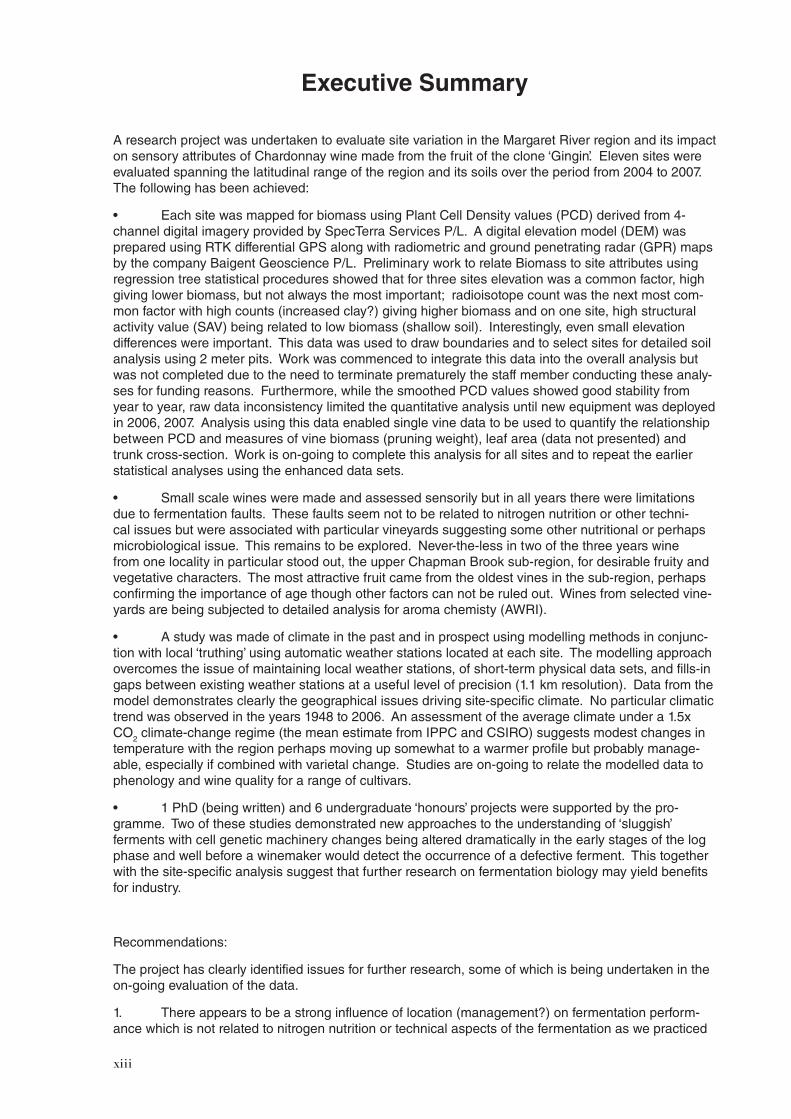
Executive Summary
A research project was undertaken to evaluate site variation in the Margaret River region and its impact on sensory attributes of Chardonnay wine made from the fruit of the clone ‘Gingin’. Eleven sites were evaluated spanning the latitudinal range of the region and its soils over the period from 2004 to 2007. The following has been achieved:
• Each site was mapped for biomass using Plant Cell Density values (PCD) derived from 4-channel digital imagery provided by SpecTerra Services P/L. A digital elevation model (DEM) was prepared using RTK differential GPS along with radiometric and ground penetrating radar (GPR) maps by the company Baigent Geoscience P/L. Preliminary work to relate Biomass to site attributes using regression tree statistical procedures showed that for three sites elevation was a common factor, high giving lower biomass, but not always the most important; radioisotope count was the next most com-mon factor with high counts (increased clay?) giving higher biomass and on one site, high structural activity value (SAV) being related to low biomass (shallow soil). Interestingly, even small elevation differences were important. This data was used to draw boundaries and to select sites for detailed soil analysis using 2 meter pits. Work was commenced to integrate this data into the overall analysis but was not completed due to the need to terminate prematurely the staff member conducting these analy-ses for funding reasons. Furthermore, while the smoothed PCD values showed good stability from year to year, raw data inconsistency limited the quantitative analysis until new equipment was deployed in 2006, 2007. Analysis using this data enabled single vine data to be used to quantify the relationship between PCD and measures of vine biomass (pruning weight), leaf area (data not presented) and trunk cross-section. Work is on-going to complete this analysis for all sites and to repeat the earlier statistical analyses using the enhanced data sets.
• Small scale wines were made and assessed sensorily but in all years there were limitations due to fermentation faults. These faults seem not to be related to nitrogen nutrition or other techni-cal issues but were associated with particular vineyards suggesting some other nutritional or perhaps microbiological issue. This remains to be explored. Never-the-less in two of the three years wine from one locality in particular stood out, the upper Chapman Brook sub-region, for desirable fruity and vegetative characters. The most attractive fruit came from the oldest vines in the sub-region, perhaps confirming the importance of age though other factors can not be ruled out. Wines from selected vine-yards are being subjected to detailed analysis for aroma chemisty (AWRI).
• A study was made of climate in the past and in prospect using modelling methods in conjunc-tion with local ‘truthing’ using automatic weather stations located at each site. The modelling approach overcomes the issue of maintaining local weather stations, of short-term physical data sets, and fills-in gaps between existing weather stations at a useful level of precision (1.1 km resolution). Data from the model demonstrates clearly the geographical issues driving site-specific climate. No particular climatic trend was observed in the years 1948 to 2006. An assessment of the average climate under a 1.5x CO2 climate-change regime (the mean estimate from IPPC and CSIRO) suggests modest changes in temperature with the region perhaps moving up somewhat to a warmer profile but probably manage-able, especially if combined with varietal change. Studies are on-going to relate the modelled data to phenology and wine quality for a range of cultivars.
• 1 PhD (being written) and 6 undergraduate ‘honours’ projects were supported by the pro-gramme. Two of these studies demonstrated new approaches to the understanding of ‘sluggish’ ferments with cell genetic machinery changes being altered dramatically in the early stages of the log phase and well before a winemaker would detect the occurrence of a defective ferment. This together with the site-specific analysis suggest that further research on fermentation biology may yield benefits for industry.
Recommendations:
The project has clearly identified issues for further research, some of which is being undertaken in the on-going evaluation of the data.
1. There appears to be a strong influence of location (management?) on fermentation perform-ance which is not related to nitrogen nutrition or technical aspects of the fermentation as we practiced

xiv
it.
2. A new approach to ‘ground-truthing’ remotely sensed biomass has been proposed. Evaluation of this is on-going but should provide a method for relating individual vine biomass to remotely sensed imagery values (PCD or soil and land form).
3. Three site factors were shown to be well related to vine biomass for three of the sites: elevation ( ve); radiometric count (+ve) and depth to hardpan (SAV) (+ve). Work is on-going to complete these analyses for the remaining sites.
4. Trunk diameter is proposed as a simple system for estimating vine biomass variation within particular sites. Cane cross section also provides a useful, non-destructive way of estimating leaf area though pruning weight may also be used though this measure is more site specific. It is likely that both measures will need independent calibration for particular cultivars.
5. The modelling approach developed for mapping climate is being applied to other regions within WA and prospectively could be a useful tool for all regions, minimising the need for individual weather stations. The techniques has been used to model climate for Margaret River under a climate change regime and work is in progress to model the prospective impact on vine phenology and wine quality.
6. In the years of vine-monitoring there was evidence of a general increase in vine biomass and for rigid vine management, rather than adaptive management leading to vines pruned sub-optimally and to reduced functional fertility. Improved training for farm hands could lead to more optimal prun-ing that takes account of within block variation and to higher levels of flower initiation which in a few instances was seriously low. In no instance was the average flower initiation at optimal levels though it was close to that in some vineyards.
John A Considine 20/04/2008
Page – 1
Environment & Chardonnay
Site characteristics: A. Soil Geoscience
Contributing Authors:
M. Baigent, J. Doedens, Baigent GeoSciences J.A. Considine School of Plant Biology, The Uni-versity of Western Australia, Crawley 6009
Abstract
This section reports the methods and data collected as part of the site charac-terisation studies. Each site was simultaneously mapped by differential GPS, ground penetrating radar (GPR) and gamma radiation. The GPS was to provide precise location details and to produce a digital elevation model (DEM) for sub-sequent use in conjunction with a regional DEM. The GPR was acquired for the purpose of establishing boundaries that might be related to commercially avail-able remotely sensed biomass indices (e.g. plant cell density maps, PCD) and gamma radiation as a way of estimating the chemistry and origin of the surface soil (potassium, thorium and uranium isotopes).
The GPR and radiometric data provided maps that display the gradients and boundaries of the surface and underlying soils, variations that are not always readily apparent to the eye.
IntroductionThe primary purpose of this survey was to demonstrate the effectiveness of the use of Ground Penetrating Radar (GPR) as a tool for identifying the predominant soil horizons and the depths at which they occur. Soil is well known as a key variable in site selection and site management.
In conjunction with this, radiometric data was collected in order to broadly classify soil types with similar mineral properties.
Terminology
GPR Ground Penetrating Radar
GPS Global Positioning System
WGS84 World Geodetic System 1984
MGA Map Grid of Australia
GDA Geodetic Datum of Australia
SAV Structural Activity Value
Materials & MethodsSurvey Specifications: The sample intervals and speed determine the resolution of the im-ages. These differ from each other and from the aerial imagery provided by SpecTerra P/L. For comparison purposes, examples of Plant Cell Density Images (unclassified) and visual spectrum images (RGB) are also included (source SpecTerra Services Ltd).
Environment & Chardonnay
Page – 2
DATA ACQUISITION SPECIFICATIONS
Ground Penetrating Radar :
Sample Interval 0.2 sec ( approx 0.66 metres)
Line Spacing 3 metres
Radiometrics :
Sample Interval 2 sec (approx 4.0 metres)
Line Spacing 3 metres
Vehicle Speed 12.0 Km/h ( 3.33 metres/sec)
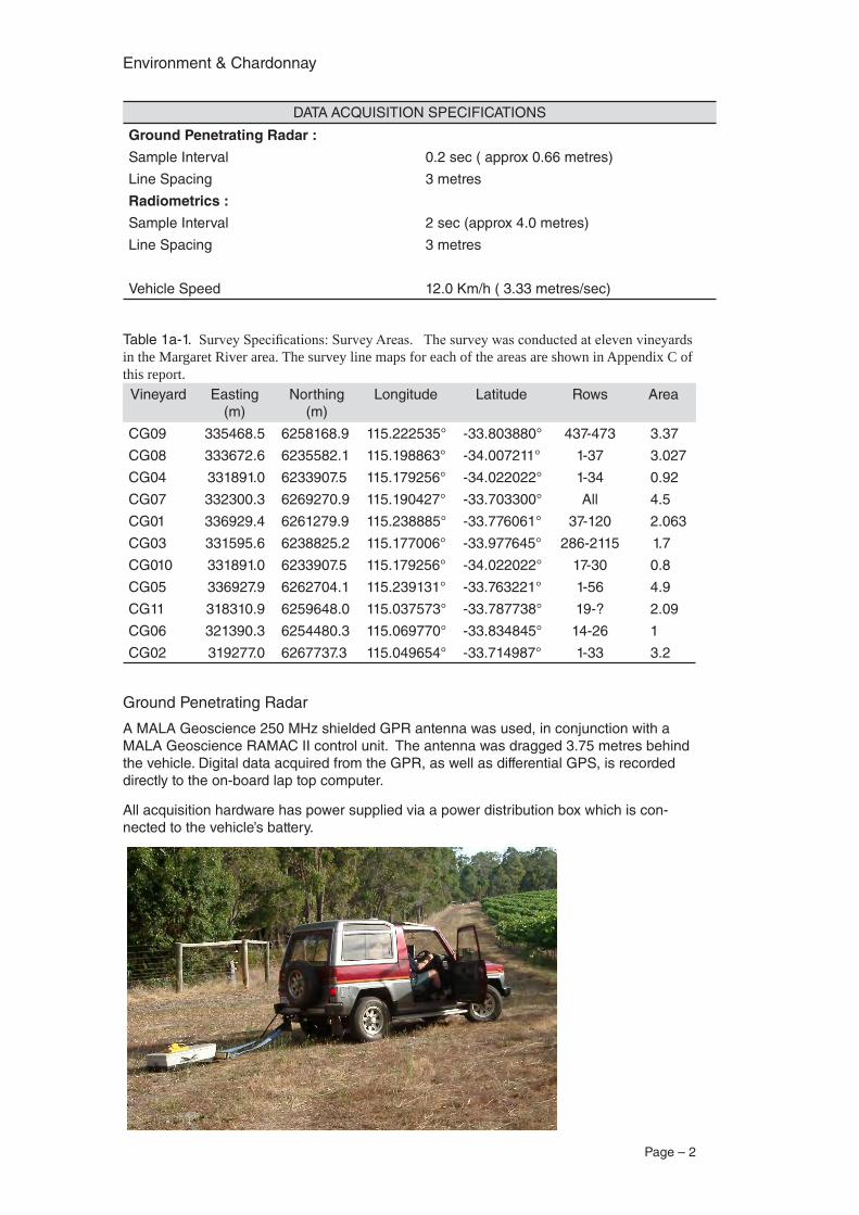
Table 1a-1. Survey Specifications: Survey Areas. The survey was conducted at eleven vineyards in the Margaret River area. The survey line maps for each of the areas are shown in Appendix C of this report.Vineyard Easting
(m)Northing
(m)Longitude Latitude Rows Area
CG09 335468.5 6258168.9 115.222535° -33.803880° 437-473 3.37
CG08 333672.6 6235582.1 115.198863° -34.007211° 1-37 3.027
CG04 331891.0 6233907.5 115.179256° -34.022022° 1-34 0.92
CG07 332300.3 6269270.9 115.190427° -33.703300° All 4.5
CG01 336929.4 6261279.9 115.238885° -33.776061° 37-120 2.063
CG03 331595.6 6238825.2 115.177006° -33.977645° 286-2115 1.7
CG010 331891.0 6233907.5 115.179256° -34.022022° 17-30 0.8
CG05 336927.9 6262704.1 115.239131° -33.763221° 1-56 4.9
CG11 318310.9 6259648.0 115.037573° -33.787738° 19-? 2.09
CG06 321390.3 6254480.3 115.069770° -33.834845° 14-26 1
CG02 319277.0 6267737.3 115.049654° -33.714987° 1-33 3.2
Ground Penetrating Radar
A MALA Geoscience 250 MHz shielded GPR antenna was used, in conjunction with a MALA Geoscience RAMAC II control unit. The antenna was dragged 3.75 metres behind the vehicle. Digital data acquired from the GPR, as well as differential GPS, is recorded directly to the on-board lap top computer.
All acquisition hardware has power supplied via a power distribution box which is con-nected to the vehicle’s battery.
Page – 3
Environment & Chardonnay
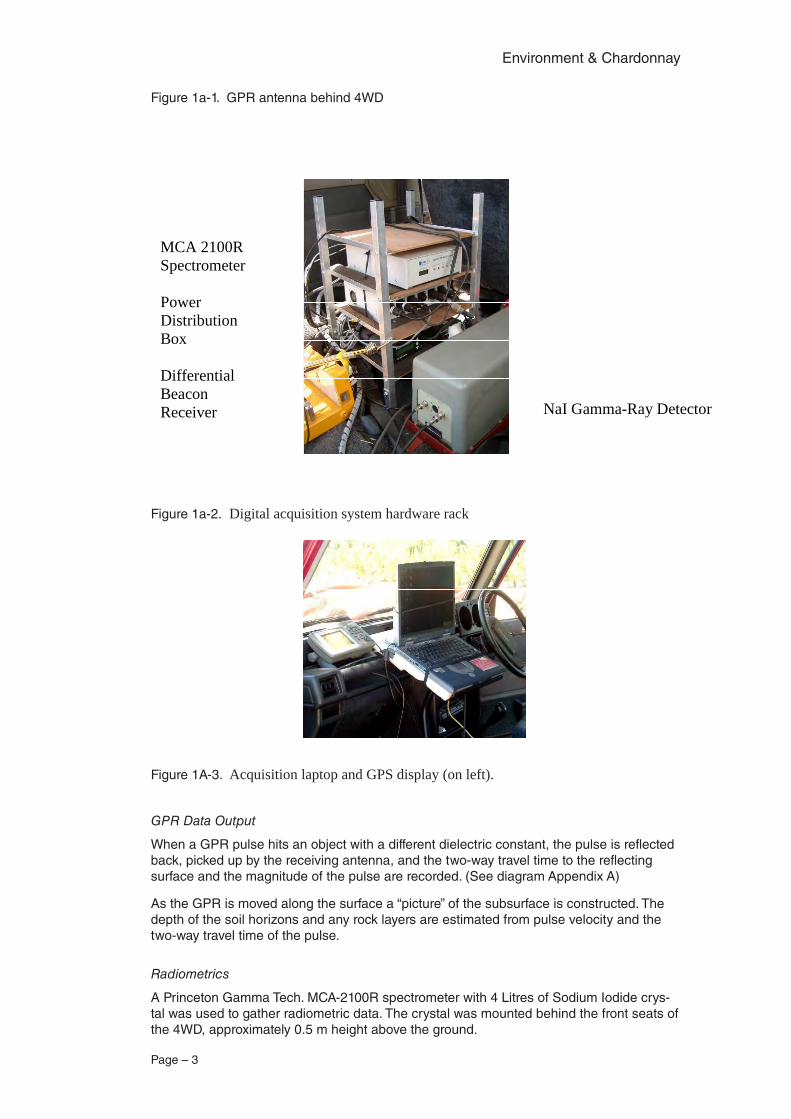
Figure 1a-1. GPR antenna behind 4WD
MCA 2100R Spectrometer Power Distribution Box Differential Beacon Receiver RAMAC II GPR Controller
NaI Gamma-Ray Detector
Figure 1a-2. Digital acquisition system hardware rack
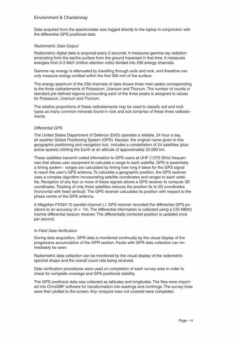
Figure 1A-3. Acquisition laptop and GPS display (on left).
GPR Data Output
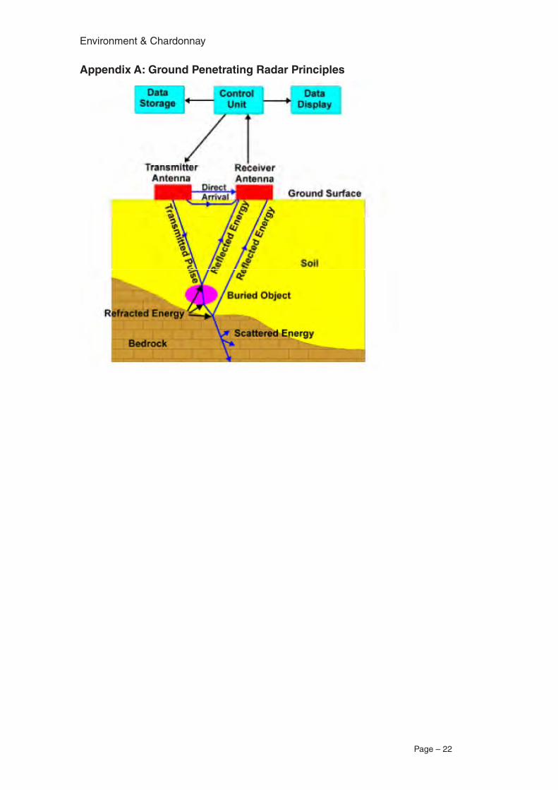
When a GPR pulse hits an object with a different dielectric constant, the pulse is reflected back, picked up by the receiving antenna, and the two-way travel time to the reflecting surface and the magnitude of the pulse are recorded. (See diagram Appendix A)
As the GPR is moved along the surface a “picture” of the subsurface is constructed. The depth of the soil horizons and any rock layers are estimated from pulse velocity and the two-way travel time of the pulse.
Radiometrics
A Princeton Gamma Tech. MCA-2100R spectrometer with 4 Litres of Sodium Iodide crys-tal was used to gather radiometric data. The crystal was mounted behind the front seats of the 4WD, approximately 0.5 m height above the ground.
Environment & Chardonnay
Page – 4
Data acquired from the spectrometer was logged directly to the laptop in conjunction with the differential GPS positional data.
Radiometric Data Output
Radiometric digital data is acquired every 2 seconds. It measures gamma-ray radiation emanating from the earths surface from the ground traversed in that time. It measures energies from 0-3 MeV (million electron volts) divided into 256 energy channels.
Gamma-ray energy is attenuated by travelling through soils and rock, and therefore can only measure energy emitted within the first 300 mm of the surface.
The energy spectrum of the 256 channels of data shows three main peaks corresponding to the three radioelements of Potassium, Uranium and Thorium. The number of counts in standard pre-defined regions surrounding each of the three peaks is assigned to values for Potassium, Uranium and Thorium.
The relative proportions of these radioelements may be used to classify soil and rock types as many common minerals found in rock and soil comprise of these three radioele-ments.
Differential GPS
The United States Department of Defence (DoD) operates a reliable, 24 hour a day, all weather Global Positioning System (GPS). Navstar, the original name given to this geographic positioning and navigation tool, includes a constellation of 24 satellites (plus active spares) orbiting the Earth at an altitude of approximately 22,000 km.
These satellites transmit coded information to GPS users at UHF (1.575 GHz) frequen-cies that allows user equipment to calculate a range to each satellite. GPS is essentially a timing system - ranges are calculated by timing how long it takes for the GPS signal to reach the user’s GPS antenna. To calculate a geographic position, the GPS receiver uses a complex algorithm incorporating satellite coordinates and ranges to each satel-lite. Reception of any four or more of these signals allows a GPS receiver to compute 3D coordinates. Tracking of only three satellites reduces the position fix to 2D coordinates (horizontal with fixed vertical). The GPS receiver calculates its position with respect to the phase centre of the GPS antenna.
A Magellan FX324 12 parallel channel L1 GPS receiver recorded the differential GPS po-sitions to an accuracy of +- 1m. The differential information is collected using a CSI MBX3 marine differential beacon receiver. The differentially corrected position is updated once per second.
In-Field Data Verification
During data acquisition, GPR data is monitored continually by the visual display of the progressive accumulation of the GPR section. Faults with GPR data collection can im-mediately be seen.
Radiometric data collection can be monitored by the visual display of the radiometric spectral shape and the overall count rate being received.
Data verification procedures were used on completion of each survey area in order to check for complete coverage and GPS positional stability.
The GPS positional data was collected as latitudes and longitudes. The files were import-ed into ChrisDBF software for transformation into eastings and northings. The survey lines were then plotted to the screen. Any vineyard rows not covered were completed.
Page – 5
Environment & Chardonnay
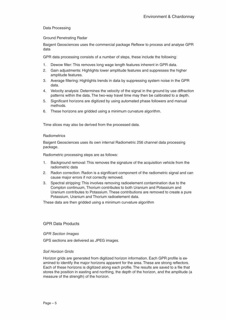
Data Processing
Ground Penetrating Radar
Baigent Geosciences uses the commercial package Reflexw to process and analyse GPR data
GPR data processing consists of a number of steps, these include the following:
Dewow filter: This removes long wage length features inherent in GPR data.
Gain adjustments: Highlights lower amplitude features and suppresses the higher amplitude features.
Average filtering: Highlights trends in data by suppressing system noise in the GPR data.
Velocity analysis: Determines the velocity of the signal in the ground by use diffraction patterns within the data. The two-way travel time may then be calibrated to a depth.
Significant horizons are digitized by using automated phase followers and manual methods.
These horizons are gridded using a minimum curvature algorithm.
Time slices may also be derived from the processed data.
Radiometrics
Baigent Geosciences uses its own internal Radiometric 256 channel data processing package.
Radiometric processing steps are as follows:
Background removal: This removes the signature of the acquisition vehicle from the radiometric data
Radon correction: Radon is a significant component of the radiometric signal and can cause major errors if not correctly removed.
Spectral stripping: This involves removing radioelement contamination due to the Compton continuum, Thorium contributes to both Uranium and Potassium and Uranium contributes to Potassium. These contributions are removed to create a pure Potassium, Uranium and Thorium radioelement data.
These data are then gridded using a minimum curvature algorithm
GPR Data Products
GPR Section Images
GPS sections are delivered as JPEG images.
Soil Horizon Grids
Horizon grids are generated from digitized horizon information. Each GPR profile is ex-amined to identify the major horizons apparent for the area. These are strong reflectors. Each of these horizons is digitized along each profile. The results are saved to a file that stores the position in easting and northing, the depth of the horizon, and the amplitude (a measure of the strength) of the horizon.
1.
2.
3.
4.
5.
6.
1.
2.
3.
Environment & Chardonnay
Page – 6
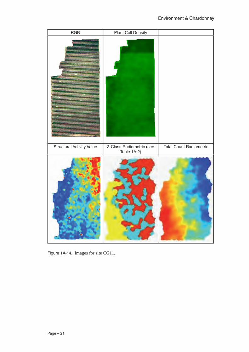
Structural Activity Value (SAV) Grid
The SAV (sometimes known as reflection density index) is a measure of the number of predominant hard reflectors. Higher grid values indicate more reflectors. Strong reflectors are usually due to the presence of rock. Rock may be present as boulders, solid bedrock or pebbly areas such as old stream beds. In the image displays, red represent a high incidence of reflectors and blue represents a low incidence.
Some strong linear features which appear may be due to reflections from irrigation pipes.
Radiometric Data Products
Radiometric Grids
Potassium
Uranium
Thorium
Total Count
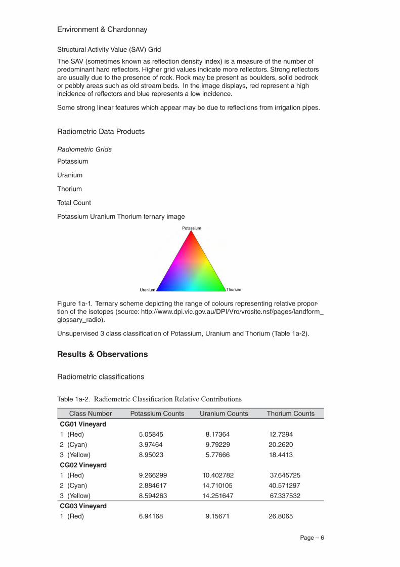
Potassium Uranium Thorium ternary image
Figure 1a-1. Ternary scheme depicting the range of colours representing relative propor-tion of the isotopes (source: http://www.dpi.vic.gov.au/DPI/Vro/vrosite.nsf/pages/landform_glossary_radio).
Unsupervised 3 class classification of Potassium, Uranium and Thorium (Table 1a-2).
Results & Observations
Radiometric classifications
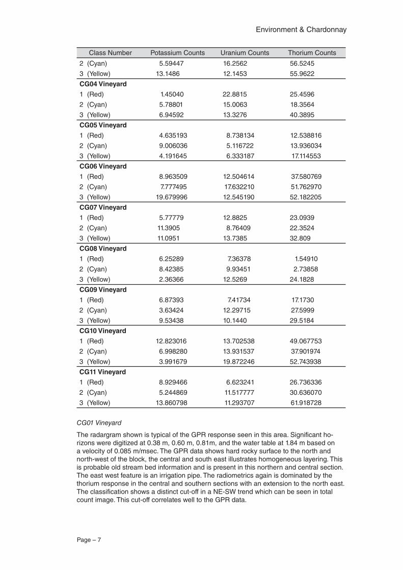
Table 1a-2. Radiometric Classification Relative Contributions
Class Number Potassium Counts Uranium Counts Thorium Counts
CG01 Vineyard
1 (Red) 5.05845 8.17364 12.7294
2 (Cyan) 3.97464 9.79229 20.2620
3 (Yellow) 8.95023 5.77666 18.4413
CG02 Vineyard
1 (Red) 9.266299 10.402782 37.645725
2 (Cyan) 2.884617 14.710105 40.571297
3 (Yellow) 8.594263 14.251647 67.337532
CG03 Vineyard
1 (Red) 6.94168 9.15671 26.8065
Page – 7
Environment & Chardonnay
Class Number Potassium Counts Uranium Counts Thorium Counts
2 (Cyan) 5.59447 16.2562 56.5245
3 (Yellow) 13.1486 12.1453 55.9622
CG04 Vineyard
1 (Red) 1.45040 22.8815 25.4596
2 (Cyan) 5.78801 15.0063 18.3564
3 (Yellow) 6.94592 13.3276 40.3895
CG05 Vineyard
1 (Red) 4.635193 8.738134 12.538816
2 (Cyan) 9.006036 5.116722 13.936034
3 (Yellow) 4.191645 6.333187 17.114553
CG06 Vineyard
1 (Red) 8.963509 12.504614 37.580769
2 (Cyan) 7.777495 17.632210 51.762970
3 (Yellow) 19.679996 12.545190 52.182205
CG07 Vineyard
1 (Red) 5.77779 12.8825 23.0939
2 (Cyan) 11.3905 8.76409 22.3524
3 (Yellow) 11.0951 13.7385 32.809
CG08 Vineyard
1 (Red) 6.25289 7.36378 1.54910
2 (Cyan) 8.42385 9.93451 2.73858
3 (Yellow) 2.36366 12.5269 24.1828
CG09 Vineyard
1 (Red) 6.87393 7.41734 17.1730
2 (Cyan) 3.63424 12.29715 27.5999
3 (Yellow) 9.53438 10.1440 29.5184
CG10 Vineyard
1 (Red) 12.823016 13.702538 49.067753
2 (Cyan) 6.998280 13.931537 37.901974
3 (Yellow) 3.991679 19.872246 52.743938
CG11 Vineyard
1 (Red) 8.929466 6.623241 26.736336
2 (Cyan) 5.244869 11.517777 30.636070
3 (Yellow) 13.860798 11.293707 61.918728
CG01 Vineyard
The radargram shown is typical of the GPR response seen in this area. Significant ho-rizons were digitized at 0.38 m, 0.60 m, 0.81m, and the water table at 1.84 m based on a velocity of 0.085 m/msec. The GPR data shows hard rocky surface to the north and north-west of the block, the central and south east illustrates homogeneous layering. This is probable old stream bed information and is present in this northern and central section. The east west feature is an irrigation pipe. The radiometrics again is dominated by the thorium response in the central and southern sections with an extension to the north east. The classification shows a distinct cut-off in a NE-SW trend which can be seen in total count image. This cut-off correlates well to the GPR data.
Environment & Chardonnay
Page – 8
CG01
CG03
CG05
CG07
CG09
CG11
CG02
CG04
CG06
CG08
CG10
Figure 1a-4. Representative radargrams from each site. The horizontal scale is in Meters and the vertical is in nanoseconds corresponding to a depth of from zero (upper surface) to nearly 6 meters.
Page – 9
Environment & Chardonnay
CG02 Vineyard
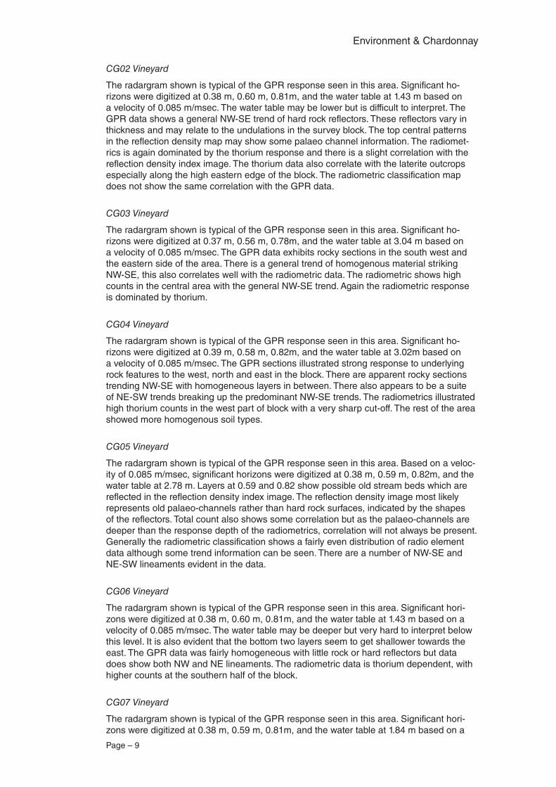
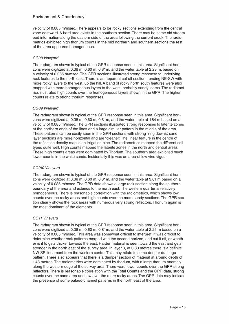
The radargram shown is typical of the GPR response seen in this area. Significant ho-rizons were digitized at 0.38 m, 0.60 m, 0.81m, and the water table at 1.43 m based on a velocity of 0.085 m/msec. The water table may be lower but is difficult to interpret. The GPR data shows a general NW-SE trend of hard rock reflectors. These reflectors vary in thickness and may relate to the undulations in the survey block. The top central patterns in the reflection density map may show some palaeo channel information. The radiomet-rics is again dominated by the thorium response and there is a slight correlation with the reflection density index image. The thorium data also correlate with the laterite outcrops especially along the high eastern edge of the block. The radiometric classification map does not show the same correlation with the GPR data.
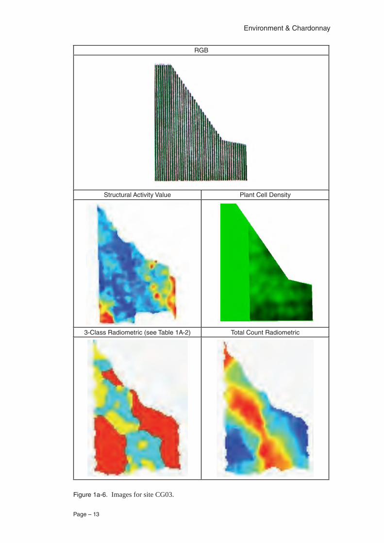
CG03 Vineyard
The radargram shown is typical of the GPR response seen in this area. Significant ho-rizons were digitized at 0.37 m, 0.56 m, 0.78m, and the water table at 3.04 m based on a velocity of 0.085 m/msec. The GPR data exhibits rocky sections in the south west and the eastern side of the area. There is a general trend of homogenous material striking NW-SE, this also correlates well with the radiometric data. The radiometric shows high counts in the central area with the general NW-SE trend. Again the radiometric response is dominated by thorium.
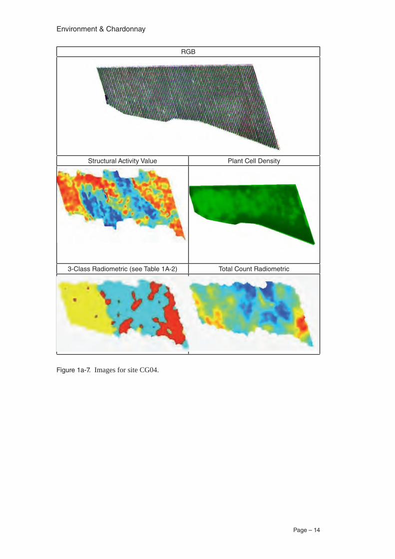
CG04 Vineyard
The radargram shown is typical of the GPR response seen in this area. Significant ho-rizons were digitized at 0.39 m, 0.58 m, 0.82m, and the water table at 3.02m based on a velocity of 0.085 m/msec. The GPR sections illustrated strong response to underlying rock features to the west, north and east in the block. There are apparent rocky sections trending NW-SE with homogeneous layers in between. There also appears to be a suite of NE-SW trends breaking up the predominant NW-SE trends. The radiometrics illustrated high thorium counts in the west part of block with a very sharp cut-off. The rest of the area showed more homogenous soil types.
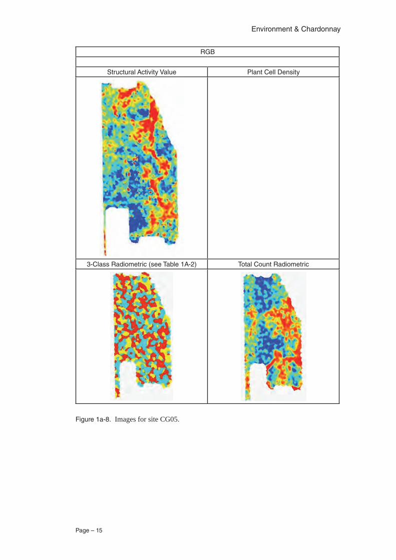
CG05 Vineyard
The radargram shown is typical of the GPR response seen in this area. Based on a veloc-ity of 0.085 m/msec, significant horizons were digitized at 0.38 m, 0.59 m, 0.82m, and the water table at 2.78 m. Layers at 0.59 and 0.82 show possible old stream beds which are reflected in the reflection density index image. The reflection density image most likely represents old palaeo-channels rather than hard rock surfaces, indicated by the shapes of the reflectors. Total count also shows some correlation but as the palaeo-channels are deeper than the response depth of the radiometrics, correlation will not always be present. Generally the radiometric classification shows a fairly even distribution of radio element data although some trend information can be seen. There are a number of NW-SE and NE-SW lineaments evident in the data.
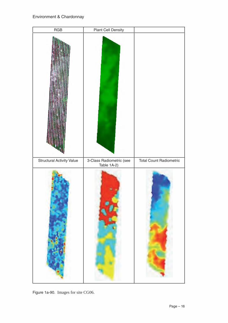
CG06 Vineyard
The radargram shown is typical of the GPR response seen in this area. Significant hori-zons were digitized at 0.38 m, 0.60 m, 0.81m, and the water table at 1.43 m based on a velocity of 0.085 m/msec. The water table may be deeper but very hard to interpret below this level. It is also evident that the bottom two layers seem to get shallower towards the east. The GPR data was fairly homogeneous with little rock or hard reflectors but data does show both NW and NE lineaments. The radiometric data is thorium dependent, with higher counts at the southern half of the block.
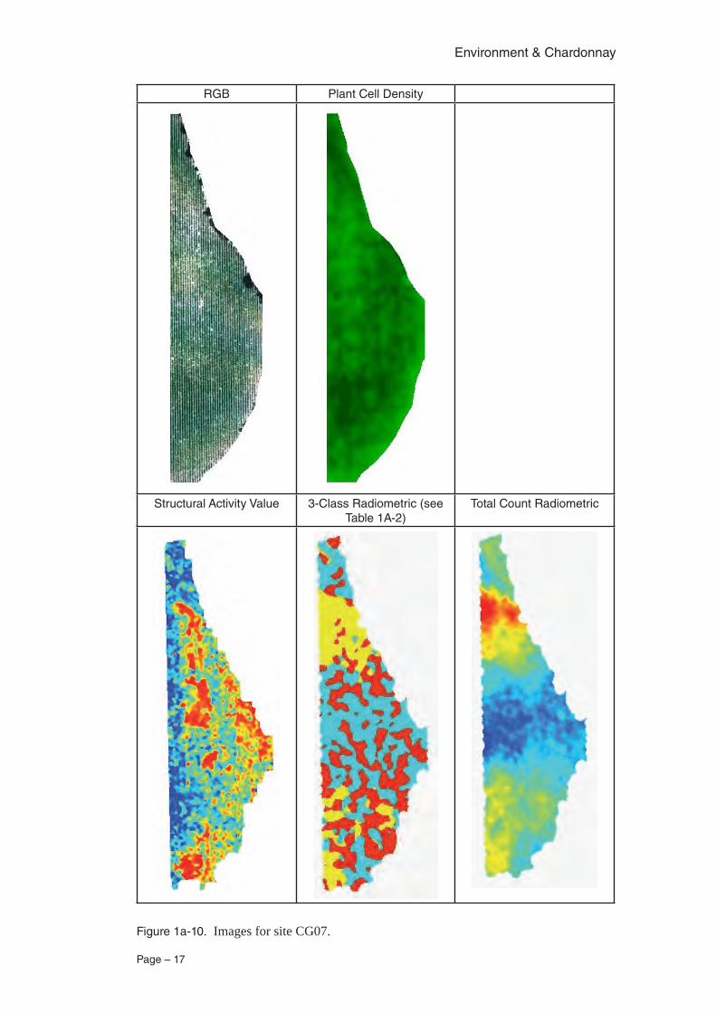
CG07 Vineyard
The radargram shown is typical of the GPR response seen in this area. Significant hori-zons were digitized at 0.38 m, 0.59 m, 0.81m, and the water table at 1.84 m based on a
Environment & Chardonnay
Page – 10
velocity of 0.085 m/msec. There appears to be rocky sections extending from the central zone eastward. A hard area exists in the southern section. There may be some old stream bed information along the eastern side of the area following the current creek. The radio-metrics exhibited high thorium counts in the mid northern and southern sections the rest of the area appeared homogeneous.
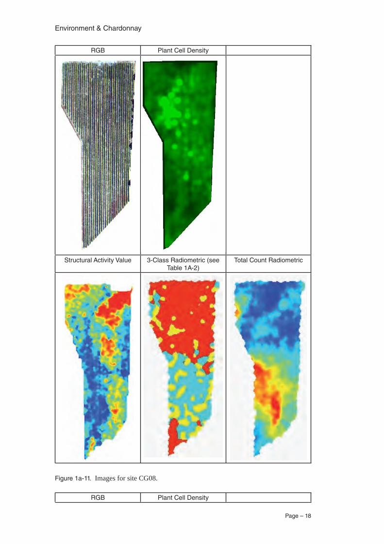
CG08 Vineyard
The radargram shown is typical of the GPR response seen in this area. Significant hori-zons were digitized at 0.38 m, 0.60 m, 0.81m, and the water table at 2.23 m. based on a velocity of 0.085 m/msec. The GPR sections illustrated strong response to underlying rock features to the north east. There is an apparent cut off section trending NE-SW with more rocky layers to the west, up the hill. A band of rocky north south features were also mapped with more homogeneous layers to the west, probably sandy loams. The radiomet-rics illustrated high counts over the homogeneous layers shown in the GPR. The higher counts relate to strong thorium responses.
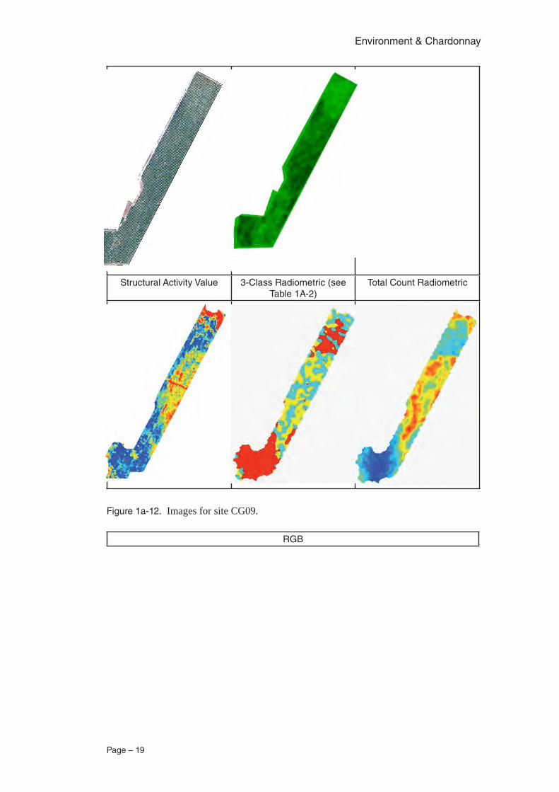
CG09 Vineyard
The radargram shown is typical of the GPR response seen in this area. Significant hori-zons were digitized at 0.38 m, 0.60 m, 0.81m, and the water table at 1.84 m based on a velocity of 0.085 m/msec. The GPR sections illustrated strong responses to laterite zones at the northern ends of the lines and a large circular pattern in the middle of the area. These patterns can be easily seen in the GPR sections with strong “ring downs”, sand layer sections are more horizontal and are “cleaner”. The linear feature in the centre of the reflection density map is an irrigation pipe. The radiometrics mapped the different soil types quite well. High counts mapped the laterite zones in the north and central areas. These high counts areas were dominated by Thorium. The southern area exhibited much lower counts in the white sands. Incidentally this was an area of low vine vigour.
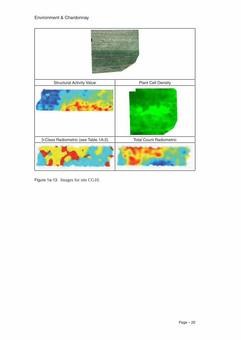
CG010 Vineyard
The radargram shown is typical of the GPR response seen in this area. Significant hori-zons were digitized at 0.38 m, 0.60 m, 0.81m, and the water table at 3.01 m based on a velocity of 0.085 m/msec. The GPR data shows a large rock section along the southern boundary of the area and extends to the north east. The western quarter is relatively homogeneous. There is reasonable correlation with the radiometrics, which shows low counts over the rocky areas and high counts over the more sandy sections. The GPR sec-tion clearly shows the rock areas with numerous very strong reflectors. Thorium again is the most dominant of the elements.
CG11 Vineyard
The radargram shown is typical of the GPR response seen in this area. Significant hori-zons were digitized at 0.38 m, 0.60 m, 0.81m, and the water table at 2.25 m based on a velocity of 0.085 m/msec. This area was somewhat difficult to interpret. It was difficult to determine whether rock patterns merged with the second horizon, and cut it off, or wheth-er is it to gets thicker towards the east. Harder material is seen toward the east and gets stronger in the north east of the survey area. In layer 3, at 0.80 metres there is a definite NW-SE lineament from the western centre. This may relate to some deeper drainage pattern. There also appears that there is a damper section of material at around depth of 1.43 metres. The radiometrics were dominated by thorium, with a large thorium anomaly along the western edge of the survey area. There were lower counts over the GPR strong reflectors. There is reasonable correlation with the Total Counts and the GPR data, strong counts over the sand area and low over the more rocky areas. The GPR data may indicate the presence of some palaeo-channel patterns in the north east of the area.
Page – 11
Environment & Chardonnay
RGB
Structural Activity Value Plant Cell Density
3-Class Radiometric (see Table 1A-2) Total Count Radiometric
Figure 1a-4. Images for site CG01.
Environment & Chardonnay
Page – 12
RGB Plant Cell Density
Structural Activity Value 3-Class Radiometric (see Table 1a-2)
Total Count Radiometric
Figure 1a-5. Images for site CG02
Page – 13
Environment & Chardonnay
RGB
Structural Activity Value Plant Cell Density
3-Class Radiometric (see Table 1A-2) Total Count Radiometric
Figure 1a-6. Images for site CG03.
Environment & Chardonnay
Page – 14
RGB
Structural Activity Value Plant Cell Density
3-Class Radiometric (see Table 1A-2) Total Count Radiometric
Figure 1a-7. Images for site CG04.
Page – 15
Environment & Chardonnay
RGB
Structural Activity Value Plant Cell Density
3-Class Radiometric (see Table 1A-2) Total Count Radiometric
Figure 1a-8. Images for site CG05.
Environment & Chardonnay
Page – 16
RGB Plant Cell Density
Structural Activity Value 3-Class Radiometric (see Table 1A-2)
Total Count Radiometric
Figure 1a-90. Images for site CG06.
Page – 17
Environment & Chardonnay
RGB Plant Cell Density
Structural Activity Value 3-Class Radiometric (see Table 1A-2)
Total Count Radiometric
Figure 1a-10. Images for site CG07.
Environment & Chardonnay
Page – 18
RGB Plant Cell Density
Structural Activity Value 3-Class Radiometric (see Table 1A-2)
Total Count Radiometric
Figure 1a-11. Images for site CG08.
RGB Plant Cell Density
Page – 19
Environment & Chardonnay
Structural Activity Value 3-Class Radiometric (see Table 1A-2)
Total Count Radiometric
Figure 1a-12. Images for site CG09.
RGB
Environment & Chardonnay
Page – 20
Structural Activity Value Plant Cell Density
3-Class Radiometric (see Table 1A-2) Total Count Radiometric
Figure 1a-13. Images for site CG10.
Page – 21
Environment & Chardonnay
RGB Plant Cell Density
Structural Activity Value 3-Class Radiometric (see Table 1A-2)
Total Count Radiometric
Figure 1A-14. Images for site CG11.
Environment & Chardonnay
Page – 22
Appendix A: Ground Penetrating Radar Principles
Page – 23
Environment & Chardonnay
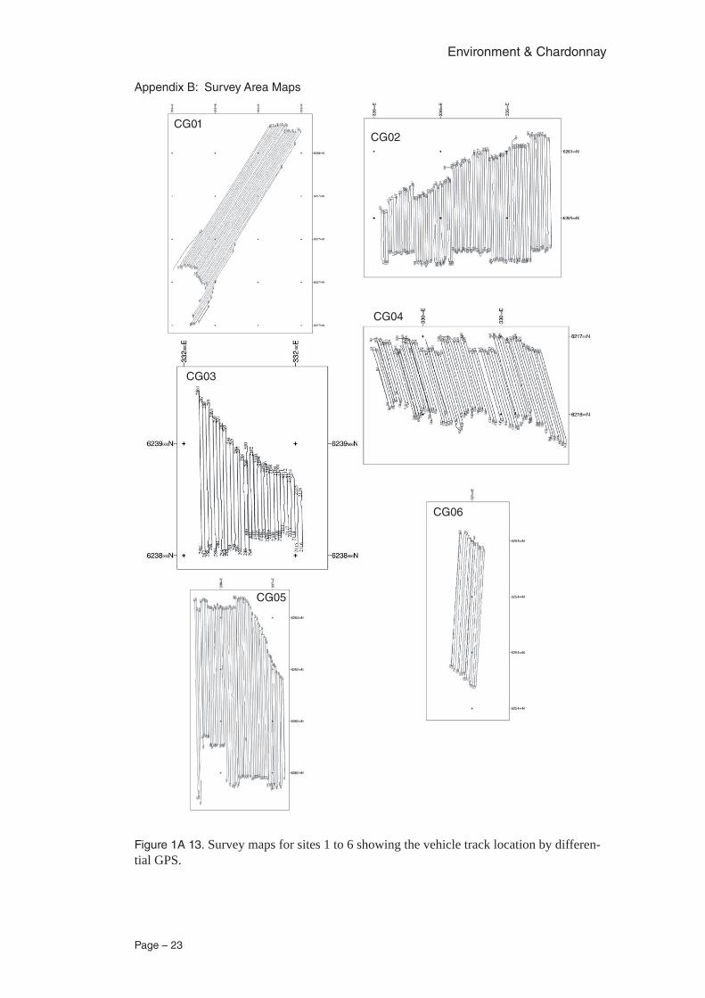
Appendix B: Survey Area Maps
CG01
CG03
CG05
CG02
CG04
CG06
Figure 1A 13. Survey maps for sites 1 to 6 showing the vehicle track location by differen-tial GPS.
Environment & Chardonnay
Page – 24
CG07 CG08
CG09CG10
CG11
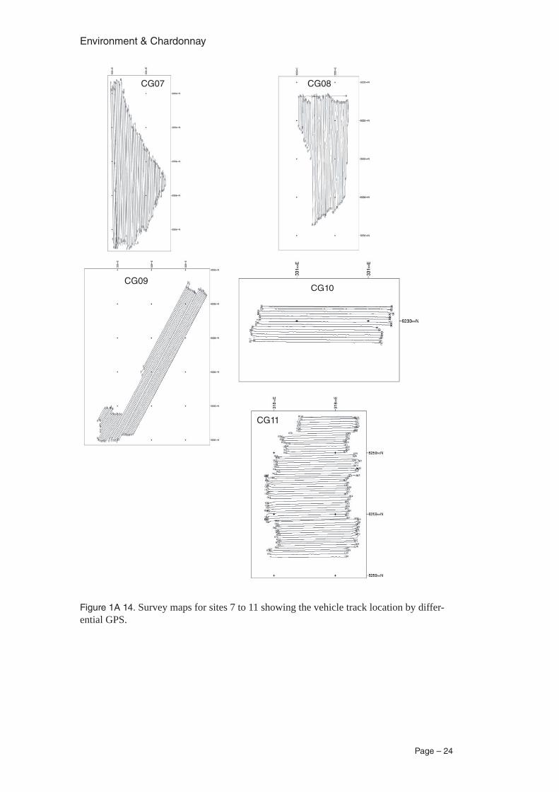
Figure 1A 14. Survey maps for sites 7 to 11 showing the vehicle track location by differ-ential GPS.
Page – 25
Environment & Chardonnay
Soil Surveys of Chardonnay Blocks
Principal Author: Dr Chris Shedley B. Sc. Agric (UWA); Ph. D (UNE), SHEDLEY CONSULTING SERVICES, RMB 382 BRIDGETOWN WA 6255, Ph: (08) 97 617 512 Email: cshedley@bigpond.
com
Contibuting Authors: Dr G. Pracilio, Dr J.A. Considine, School of Plant Biology, The University of Western Australia, Crawley 6009
M. Baigent, J Doedens, Baigent Geosciences. P/L, 7 Owsten Court, Banup, WA 6164, [email protected]
IntroductionThe object of the Project was to attempt to identify site and management factors that influ-ence the quality of Chardonnay wines produced in the Margaret River area, and hopefully to describe the nature of some of these relationships.
Eleven blocks of Chardonnay had been chosen as the study areas, and some remote sens-ing using ground based Ground Probing Radar (GPR) and Gamma Ray Spectometry (Radio-metrics) had been done on these sites by Baigent Geosciences. This task was to do physical soil profile descriptions in a number of sites in each vineyard to provide some ground-truthing to aid in calibrating and interpreting that data. Together it was intended to evaluate these techniques as an aid to developing an understanding of soil factors that may influence grape and wine quality in a number of plots on each vineyard. The project also wished to determine whether the remote sensing data was yielding useful information on soil properties that influ-ence wine quality.
ApproachThe project group at a meeting on May 16th meeting engaged me to start doing soil profile descriptions on three of the eleven properties to see if useful relationships were likely and to develop a better understanding of the variability in soils within and between sites. We chose what we thought were three quite different sites (CG01, CG08 and CG11) and located posi-tions for soil pits to cover the ranges in GPR and Radiometric data values at each site.
Soil profile descriptions were done on 15 soil pits at CG01 on 24th May 2005, on 13 pits at CG08 on 8th June 2005 and 13 pits at CG11 on 8th August 2005.
Soils were described using methodology described in “Australian Soil and Land Survey Field Handbook (McDonald, Isbell, Speight, Walker and Hopkins) 1990. Samples were taken from each horizon for physical and chemical analyses at UWA and CSBP laboratories.
Following some promising initial outcomes from these first three sites, it was decided to go ahead and describe the soils at the remaining eight sites over the summer of 2005/2006.
Results and Data
Vineyard CG01
CG01 vineyard is on the corner of Kaloorup and Adams Roads, at the junction of the Abba Plains Land System and the Yelverton Shelf Land System, Abba flats and Abba wet flats sub-systems (Tille and Lantzke 1990).
Environment & Chardonnay
Page – 26
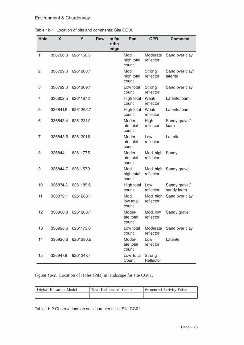
Table 1b-1. Location of pits and comments: Site CG01.
Hole X Y Row m fm nthn edge
Rad GPR Comment
1 336726.3 6261156.3 Mod high total count
Moderate reflector
Sand over clay
2 336729.0 6261208.1 Mod high total count
Strong reflector
Sand over clay/laterite
3 336762.3 6261209.1 Low total count
Strong reflector
Sand over clay
4 336802.5 6261187.2 High total count
Weak reflector
Laterite/loam
5 336841.8 6261262.7 High total count
Weak reflector
Laterite/loam
6 336843.4 6261231.9 Moder-ate total count
High relfetcor
Sandy gravel/loam
7 336843.6 6261201.9 Moder-ate total count
Low reflector
Laterite
8 336844.1 6261177.5 Moder-ate total count
Mod. high reflector
Sandy
9 336844.7 6261157.9 Mod. high total count
Mod. high reflector
Sandy gravel
10 336874.3 6261185.6 High total count
Low reflector
Sandy gravel/ sandy loam
11 336872.1 6261283.1 Mod. low total count
Mod. high reflector
Sand over clay
12 336900.8 6261208.1 Moder-ate total count
Mod. low reflector
Sandy gravel
13 336928.6 6261173.0 Low total count
Moderate reflector
Sand over clay
14 336926.6 6261286.5 Moder-ate total count
Low reflector
Laterite
15 336947.9 6261247.7 Low Total Count
Strong Reflector
Figure 1b-2. Location of Holes (Pits) in landscape for site CG01.
Digital Elevation Model Total Radiometric Count Structural Activity Value
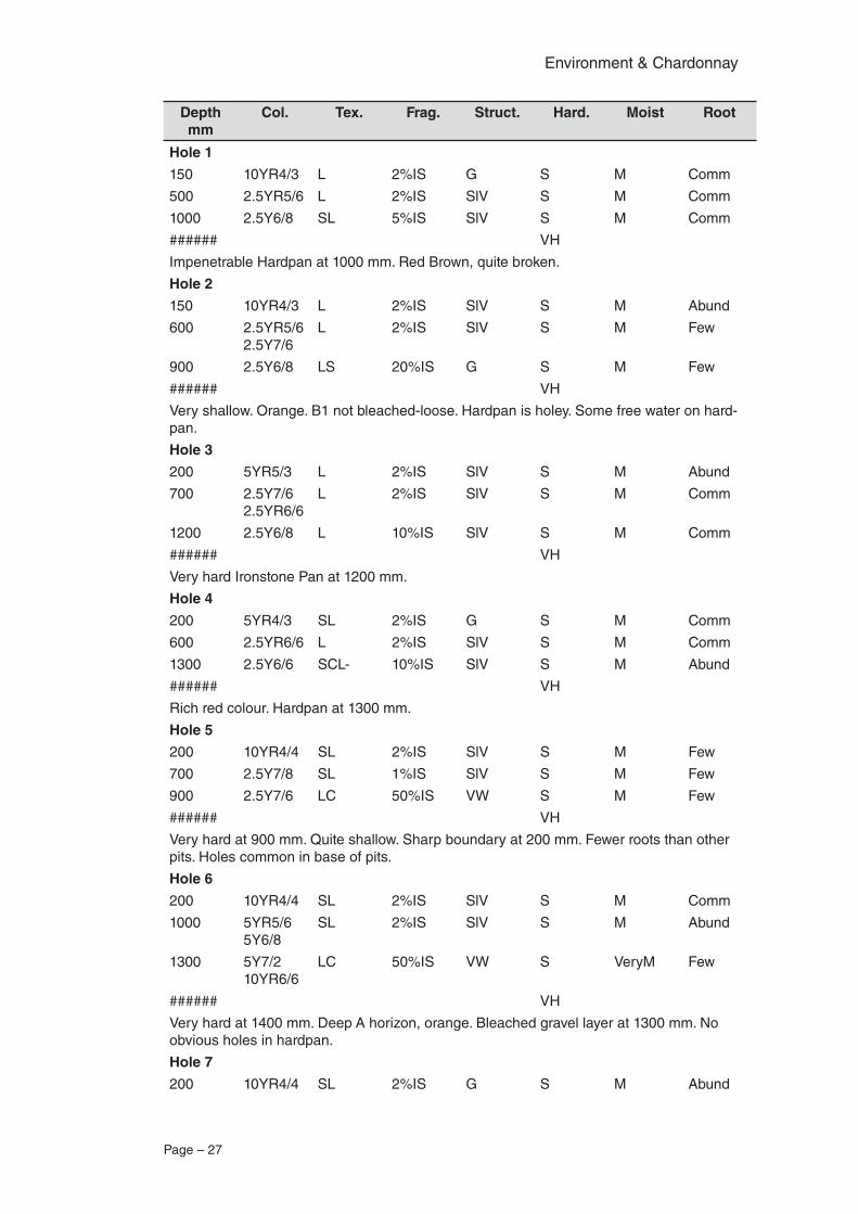
Table 1b-2 Observations on soil characteristics: Site CG01.
Page – 27
Environment & Chardonnay
Depth mm
Col. Tex. Frag. Struct. Hard. Moist Root
Hole 1
150 10YR4/3 L 2%IS G S M Comm
500 2.5YR5/6 L 2%IS SlV S M Comm
1000 2.5Y6/8 SL 5%IS SlV S M Comm
###### VH
Impenetrable Hardpan at 1000 mm. Red Brown, quite broken.
Hole 2
150 10YR4/3 L 2%IS SlV S M Abund
600 2.5YR5/6 2.5Y7/6
L 2%IS SlV S M Few
900 2.5Y6/8 LS 20%IS G S M Few
###### VH
Very shallow. Orange. B1 not bleached-loose. Hardpan is holey. Some free water on hard-pan.
Hole 3
200 5YR5/3 L 2%IS SlV S M Abund
700 2.5Y7/6 2.5YR6/6
L 2%IS SlV S M Comm
1200 2.5Y6/8 L 10%IS SlV S M Comm
###### VH
Very hard Ironstone Pan at 1200 mm.
Hole 4
200 5YR4/3 SL 2%IS G S M Comm
600 2.5YR6/6 L 2%IS SlV S M Comm
1300 2.5Y6/6 SCL- 10%IS SlV S M Abund
###### VH
Rich red colour. Hardpan at 1300 mm.
Hole 5
200 10YR4/4 SL 2%IS SlV S M Few
700 2.5Y7/8 SL 1%IS SlV S M Few
900 2.5Y7/6 LC 50%IS VW S M Few
###### VH
Very hard at 900 mm. Quite shallow. Sharp boundary at 200 mm. Fewer roots than other pits. Holes common in base of pits.
Hole 6
200 10YR4/4 SL 2%IS SlV S M Comm
1000 5YR5/6 5Y6/8
SL 2%IS SlV S M Abund
1300 5Y7/2 10YR6/6
LC 50%IS VW S VeryM Few
###### VH
Very hard at 1400 mm. Deep A horizon, orange. Bleached gravel layer at 1300 mm. No obvious holes in hardpan.
Hole 7
200 10YR4/4 SL 2%IS G S M Abund
Environment & Chardonnay
Page – 28
Depth mm
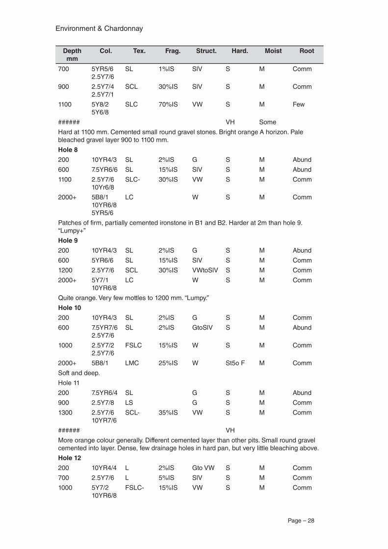
Col. Tex. Frag. Struct. Hard. Moist Root
700 5YR5/6 2.5Y7/6
SL 1%IS SlV S M Comm
900 2.5Y7/4 2.5Y7/1
SCL 30%IS SlV S M Comm
1100 5Y8/2 5Y6/8
SLC 70%IS VW S M Few
###### VH Some
Hard at 1100 mm. Cemented small round gravel stones. Bright orange A horizon. Pale bleached gravel layer 900 to 1100 mm.
Hole 8
200 10YR4/3 SL 2%IS G S M Abund
600 7.5YR6/6 SL 15%IS SlV S M Abund
1100 2.5Y7/6 10Yr6/8
SLC- 30%IS VW S M Comm
2000+ 5B8/1 10YR6/8 5YR5/6
LC W S M Comm
Patches of firm, partially cemented ironstone in B1 and B2. Harder at 2m than hole 9. “Lumpy+”
Hole 9
200 10YR4/3 SL 2%IS G S M Abund
600 5YR6/6 SL 15%IS SlV S M Comm
1200 2.5Y7/6 SCL 30%IS VWtoSlV S M Comm
2000+ 5Y7/1 10YR6/8
LC W S M Comm
Quite orange. Very few mottles to 1200 mm. “Lumpy.”
Hole 10
200 10YR4/3 SL 2%IS G S M Comm
600 7.5YR7/6 2.5Y7/6
SL 2%IS GtoSlV S M Abund
1000 2.5Y7/2 2.5Y7/6
FSLC 15%IS W S M Comm
2000+ 5B8/1 LMC 25%IS W St5o F M Comm
Soft and deep.
Hole 11
200 7.5YR6/4 SL G S M Abund
900 2.5Y7/8 LS G S M Comm
1300 2.5Y7/6 10YR7/6
SCL- 35%IS VW S M Comm
###### VH
More orange colour generally. Different cemented layer than other pits. Small round gravel cemented into layer. Dense, few drainage holes in hard pan, but very little bleaching above.
Hole 12
200 10YR4/4 L 2%IS Gto VW S M Comm
700 2.5Y7/6 L 5%IS SlV S M Comm
1000 5Y7/2 10YR6/8
FSLC- 15%IS VW S M Comm
Page – 29
Environment & Chardonnay
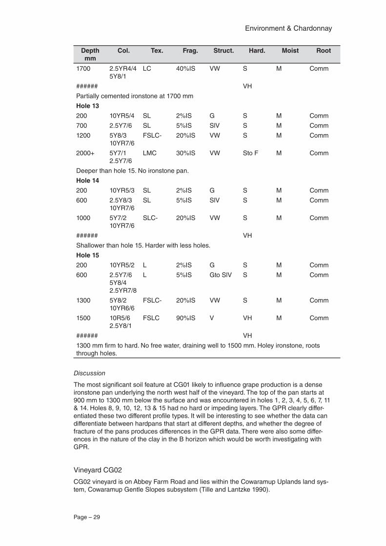
Depth mm
Col. Tex. Frag. Struct. Hard. Moist Root
1700 2.5YR4/4 5Y8/1
LC 40%IS VW S M Comm
###### VH
Partially cemented ironstone at 1700 mm
Hole 13
200 10YR5/4 SL 2%IS G S M Comm
700 2.5Y7/6 SL 5%IS SlV S M Comm
1200 5Y8/3 10YR7/6
FSLC- 20%IS VW S M Comm
2000+ 5Y7/1 2.5Y7/6
LMC 30%IS VW Sto F M Comm
Deeper than hole 15. No ironstone pan.
Hole 14
200 10YR5/3 SL 2%IS G S M Comm
600 2.5Y8/3 10YR7/6
SL 5%IS SlV S M Comm
1000 5Y7/2 10YR7/6
SLC- 20%IS VW S M Comm
###### VH
Shallower than hole 15. Harder with less holes.
Hole 15
200 10YR5/2 L 2%IS G S M Comm
600 2.5Y7/6 5Y8/4 2.5YR7/8
L 5%IS Gto SlV S M Comm
1300 5Y8/2 10YR6/6
FSLC- 20%IS VW S M Comm
1500 10R5/6 2.5Y8/1
FSLC 90%IS V VH M Comm
###### VH
1300 mm firm to hard. No free water, draining well to 1500 mm. Holey ironstone, roots through holes.
Discussion
The most significant soil feature at CG01 likely to influence grape production is a dense ironstone pan underlying the north west half of the vineyard. The top of the pan starts at 900 mm to 1300 mm below the surface and was encountered in holes 1, 2, 3, 4, 5, 6, 7, 11 & 14. Holes 8, 9, 10, 12, 13 & 15 had no hard or impeding layers. The GPR clearly differ-entiated these two different profile types. It will be interesting to see whether the data can differentiate between hardpans that start at different depths, and whether the degree of fracture of the pans produces differences in the GPR data. There were also some differ-ences in the nature of the clay in the B horizon which would be worth investigating with GPR.
Vineyard CG02
CG02 vineyard is on Abbey Farm Road and lies within the Cowaramup Uplands land sys-tem, Cowaramup Gentle Slopes subsystem (Tille and Lantzke 1990).
Environment & Chardonnay
Page – 30
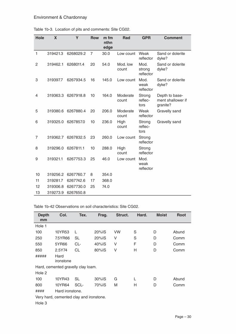
Table 1b-3. Location of pits and comments: Site CG02.
Hole X Y Row m fm nthn edge
Rad GPR Comment
1 319421.3 6268029.2 7 30.0 Low count Weak reflector
Sand or dolerite dyke?
2 319462.1 6268011.4 20 54.0 Mod. low count
Mod. strong reflector
Sand or dolerite dyke?
3 319397.7 6267934.5 16 145.0 Low count Mod. weak reflector
Sand or dolerite dyke?
4 319363.3 6267918.8 10 164.0 Moderate count
Strong reflec-tors
Depth to base-ment shallower if granite?
5 319380.6 6267880.4 20 206.0 Moderate count
Weak reflector
Gravelly sand
6 319325.0 6267857.0 10 236.0 High count
Strong reflec-tors
Gravelly sand
7 319362.7 6267832.5 23 260.0 Low count Strong reflector
8 319296.0 6267811.1 10 288.0 High count
Strong reflector
9 319321.1 6267753.3 25 46.0 Low count Mod. weak reflector
10 319256.2 6267760.7 8 354.0
11 319281.7 6267742.6 17 368.0
12 319306.8 6267730.0 25 74.0
13 319273.9 6267650.8
Table 1b-42 Observations on soil characteristics: Site CG02.
Depth mm
Col. Tex. Frag. Struct. Hard. Moist Root
Hole 1
100 10YR53 L 20%IS VW S D Abund
250 7.5YR66 SL 20%IS V S D Comm
550 5YR66 CL- 40%IS V F D Comm
850 2.5Y74 CL 80%IS V H D Comm
##### Hard ironstone
Hard, cemented gravelly clay loam.
Hole 2
100 10YR43 SL 30%IS G L D Abund
800 10YR64 SCL- 70%IS M H D Comm
#### Hard ironstone.
Very hard, cemented clay and ironstone.
Hole 3
Page – 31
Environment & Chardonnay
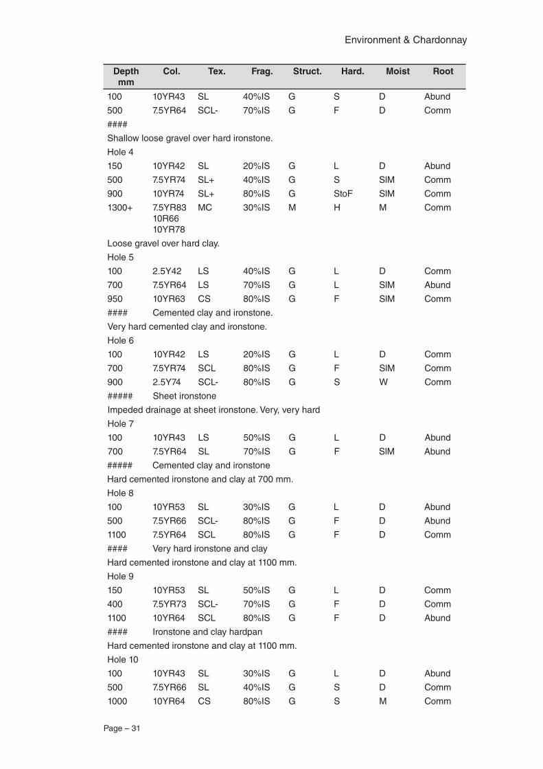
Depth mm
Col. Tex. Frag. Struct. Hard. Moist Root
100 10YR43 SL 40%IS G S D Abund
500 7.5YR64 SCL- 70%IS G F D Comm
####
Shallow loose gravel over hard ironstone.
Hole 4
150 10YR42 SL 20%IS G L D Abund
500 7.5YR74 SL+ 40%IS G S SlM Comm
900 10YR74 SL+ 80%IS G StoF SlM Comm
1300+ 7.5YR83 10R66 10YR78
MC 30%IS M H M Comm
Loose gravel over hard clay.
Hole 5
100 2.5Y42 LS 40%IS G L D Comm
700 7.5YR64 LS 70%IS G L SlM Abund
950 10YR63 CS 80%IS G F SlM Comm
#### Cemented clay and ironstone.
Very hard cemented clay and ironstone.
Hole 6
100 10YR42 LS 20%IS G L D Comm
700 7.5YR74 SCL 80%IS G F SlM Comm
900 2.5Y74 SCL- 80%IS G S W Comm
##### Sheet ironstone
Impeded drainage at sheet ironstone. Very, very hard
Hole 7
100 10YR43 LS 50%IS G L D Abund
700 7.5YR64 SL 70%IS G F SlM Abund
##### Cemented clay and ironstone
Hard cemented ironstone and clay at 700 mm.
Hole 8
100 10YR53 SL 30%IS G L D Abund
500 7.5YR66 SCL- 80%IS G F D Abund
1100 7.5YR64 SCL 80%IS G F D Comm
#### Very hard ironstone and clay
Hard cemented ironstone and clay at 1100 mm.
Hole 9
150 10YR53 SL 50%IS G L D Comm
400 7.5YR73 SCL- 70%IS G F D Comm
1100 10YR64 SCL 80%IS G F D Abund
#### Ironstone and clay hardpan
Hard cemented ironstone and clay at 1100 mm.
Hole 10
100 10YR43 SL 30%IS G L D Abund
500 7.5YR66 SL 40%IS G S D Comm
1000 10YR64 CS 80%IS G S M Comm
Environment & Chardonnay
Page – 32
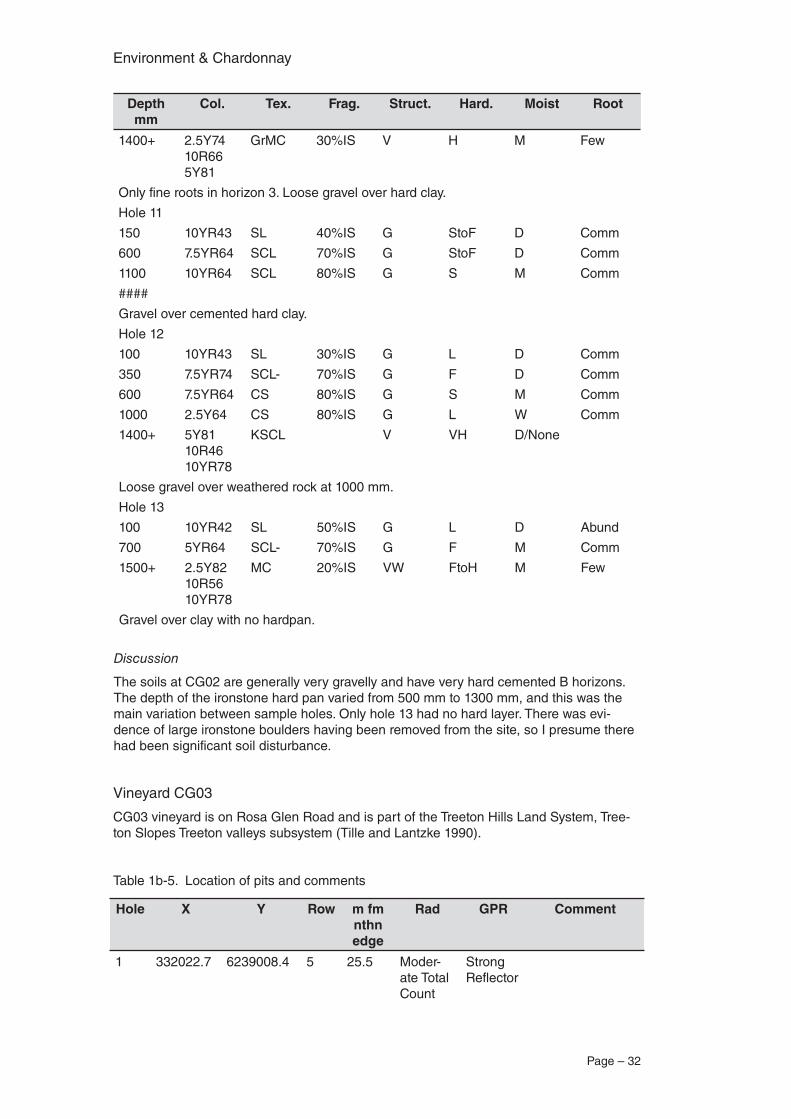
Depth mm
Col. Tex. Frag. Struct. Hard. Moist Root
1400+ 2.5Y74 10R66 5Y81
GrMC 30%IS V H M Few
Only fine roots in horizon 3. Loose gravel over hard clay.
Hole 11
150 10YR43 SL 40%IS G StoF D Comm
600 7.5YR64 SCL 70%IS G StoF D Comm
1100 10YR64 SCL 80%IS G S M Comm
####
Gravel over cemented hard clay.
Hole 12
100 10YR43 SL 30%IS G L D Comm
350 7.5YR74 SCL- 70%IS G F D Comm
600 7.5YR64 CS 80%IS G S M Comm
1000 2.5Y64 CS 80%IS G L W Comm
1400+ 5Y81 10R46 10YR78
KSCL V VH D/None
Loose gravel over weathered rock at 1000 mm.
Hole 13
100 10YR42 SL 50%IS G L D Abund
700 5YR64 SCL- 70%IS G F M Comm
1500+ 2.5Y82 10R56 10YR78
MC 20%IS VW FtoH M Few
Gravel over clay with no hardpan.
Discussion
The soils at CG02 are generally very gravelly and have very hard cemented B horizons. The depth of the ironstone hard pan varied from 500 mm to 1300 mm, and this was the main variation between sample holes. Only hole 13 had no hard layer. There was evi-dence of large ironstone boulders having been removed from the site, so I presume there had been significant soil disturbance.
Vineyard CG03
CG03 vineyard is on Rosa Glen Road and is part of the Treeton Hills Land System, Tree-ton Slopes Treeton valleys subsystem (Tille and Lantzke 1990).
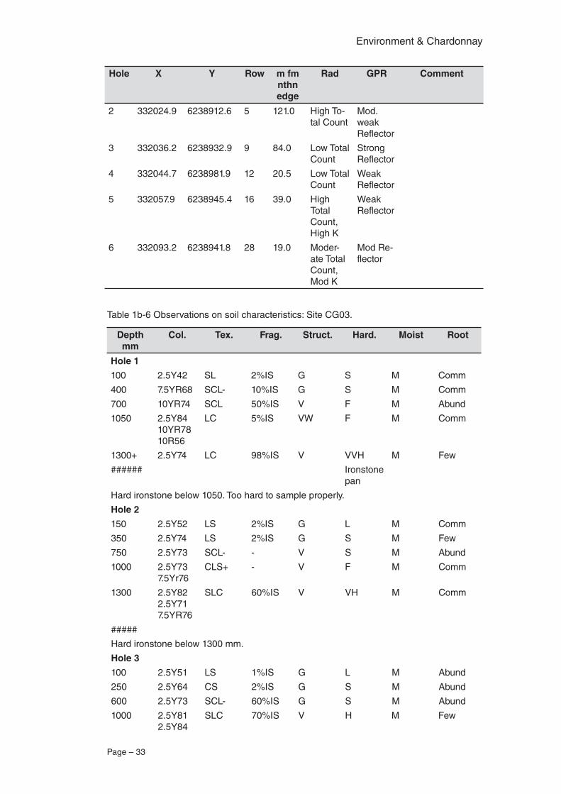
Table 1b-5. Location of pits and comments
Hole X Y Row m fm nthn edge
Rad GPR Comment
1 332022.7 6239008.4 5 25.5 Moder-ate Total Count
Strong Reflector
Page – 33
Environment & Chardonnay
Hole X Y Row m fm nthn edge
Rad GPR Comment
2 332024.9 6238912.6 5 121.0 High To-tal Count
Mod. weak Reflector
3 332036.2 6238932.9 9 84.0 Low Total Count
Strong Reflector
4 332044.7 6238981.9 12 20.5 Low Total Count
Weak Reflector
5 332057.9 6238945.4 16 39.0 High Total Count, High K
Weak Reflector
6 332093.2 6238941.8 28 19.0 Moder-ate Total Count, Mod K
Mod Re-flector
Table 1b-6 Observations on soil characteristics: Site CG03.
Depth mm
Col. Tex. Frag. Struct. Hard. Moist Root
Hole 1
100 2.5Y42 SL 2%IS G S M Comm
400 7.5YR68 SCL- 10%IS G S M Comm
700 10YR74 SCL 50%IS V F M Abund
1050 2.5Y84 10YR78 10R56
LC 5%IS VW F M Comm
1300+ 2.5Y74 LC 98%IS V VVH M Few
###### Ironstone pan
Hard ironstone below 1050. Too hard to sample properly.
Hole 2
150 2.5Y52 LS 2%IS G L M Comm
350 2.5Y74 LS 2%IS G S M Few
750 2.5Y73 SCL- - V S M Abund
1000 2.5Y73 7.5Yr76
CLS+ - V F M Comm
1300 2.5Y82 2.5Y71 7.5YR76
SLC 60%IS V VH M Comm
#####
Hard ironstone below 1300 mm.
Hole 3
100 2.5Y51 LS 1%IS G L M Abund
250 2.5Y64 CS 2%IS G S M Abund
600 2.5Y73 SCL- 60%IS G S M Abund
1000 2.5Y81 2.5Y84
SLC 70%IS V H M Few
Environment & Chardonnay
Page – 34
Depth mm
Col. Tex. Frag. Struct. Hard. Moist Root
##### Hard ironstone
Very hard below 1000 mm.
Hole 4
150 10YR42 SL 10%IS G S M Comm
450 10YR74 10YR62
SCL 10%IS G S M Comm
900 2.5Y83 10YR78
LC 40%IS VW F M Comm
1400+ 2.5Y81 10YR68 5YR66
LC 2%IS W F M Comm
Reasonable duplex soil.
Hole 5
100 2.5Y42 SL 30% G L M Abund
350 2.5Y72 SCL- 70%IS G L M Comm
900 10YR73 SCL 70%IS G S M Abund
1200 2.5Y81 10YR78 10R54
CLS 90%IS V VH M Few
##### Hard ironstone
Some vertical sandy channels in horizon 4 with roots in.
Hole 6
100 10YR42 SL 1%IS G S M Abund
550 10YR76 LS 1%IS G S M Abund
1600+ 5Y82 SCL - V S M Abund
Deep, soft soil. Pale B horizon.
Discussion
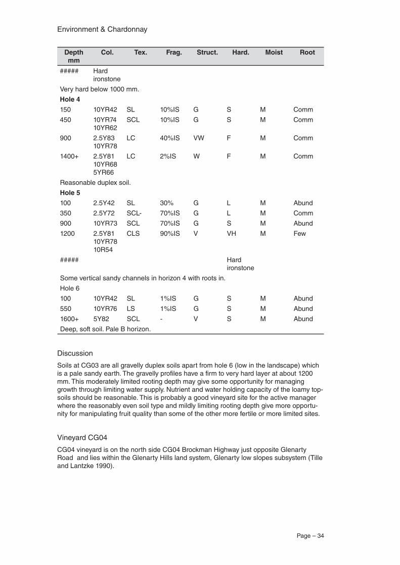
Soils at CG03 are all gravelly duplex soils apart from hole 6 (low in the landscape) which is a pale sandy earth. The gravelly profiles have a firm to very hard layer at about 1200 mm. This moderately limited rooting depth may give some opportunity for managing growth through limiting water supply. Nutrient and water holding capacity of the loamy top-soils should be reasonable. This is probably a good vineyard site for the active manager where the reasonably even soil type and mildly limiting rooting depth give more opportu-nity for manipulating fruit quality than some of the other more fertile or more limited sites.
Vineyard CG04
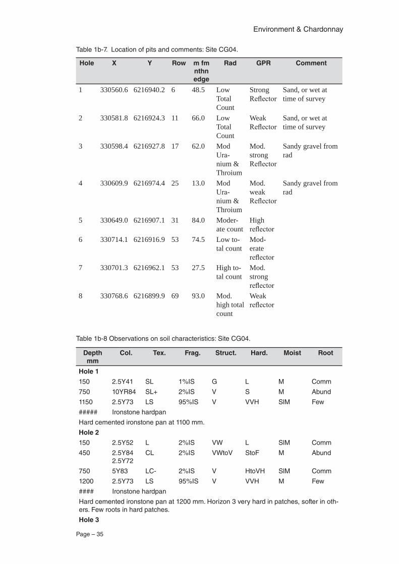
CG04 vineyard is on the north side CG04 Brockman Highway just opposite Glenarty Road and lies within the Glenarty Hills land system, Glenarty low slopes subsystem (Tille and Lantzke 1990).
Page – 35
Environment & Chardonnay
Table 1b-7. Location of pits and comments: Site CG04.
Hole X Y Row m fm nthn edge
Rad GPR Comment
1 330560.6 6216940.2 6 48.5 Low Total Count
Strong Reflector
Sand, or wet at time of survey
2 330581.8 6216924.3 11 66.0 Low Total Count
Weak Reflector
Sand, or wet at time of survey
3 330598.4 6216927.8 17 62.0 Mod Ura-nium & Throium
Mod. strong Reflector
Sandy gravel from rad
4 330609.9 6216974.4 25 13.0 Mod Ura-nium & Throium
Mod. weak Reflector
Sandy gravel from rad
5 330649.0 6216907.1 31 84.0 Moder-ate count
High reflector
6 330714.1 6216916.9 53 74.5 Low to-tal count
Mod-erate reflector
7 330701.3 6216962.1 53 27.5 High to-tal count
Mod. strong reflector
8 330768.6 6216899.9 69 93.0 Mod. high total count
Weak reflector
Table 1b-8 Observations on soil characteristics: Site CG04.
Depth mm
Col. Tex. Frag. Struct. Hard. Moist Root
Hole 1
150 2.5Y41 SL 1%IS G L M Comm
750 10YR84 SL+ 2%IS V S M Abund
1150 2.5Y73 LS 95%IS V VVH SlM Few
##### Ironstone hardpan
Hard cemented ironstone pan at 1100 mm.
Hole 2
150 2.5Y52 L 2%IS VW L SlM Comm
450 2.5Y84 2.5Y72
CL 2%IS VWtoV StoF M Abund
750 5Y83 LC- 2%IS V HtoVH SlM Comm
1200 2.5Y73 LS 95%IS V VVH M Few
#### Ironstone hardpan
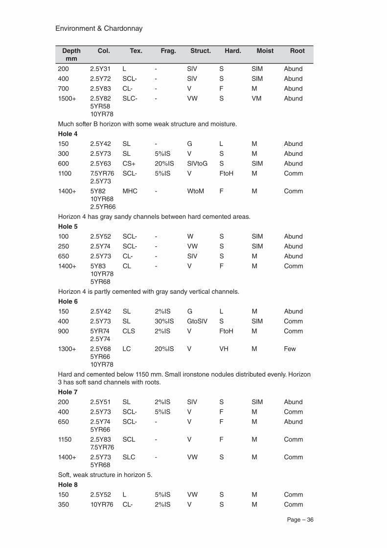
Hard cemented ironstone pan at 1200 mm. Horizon 3 very hard in patches, softer in oth-ers. Few roots in hard patches.
Hole 3
Environment & Chardonnay
Page – 36
Depth mm
Col. Tex. Frag. Struct. Hard. Moist Root
200 2.5Y31 L - SlV S SlM Abund
400 2.5Y72 SCL- - SlV S SlM Abund
700 2.5Y83 CL- - V F M Abund
1500+ 2.5Y82 5YR58 10YR78
SLC- - VW S VM Abund
Much softer B horizon with some weak structure and moisture.
Hole 4
150 2.5Y42 SL - G L M Abund
300 2.5Y73 SL 5%IS V S M Abund
600 2.5Y63 CS+ 20%IS SlVtoG S SlM Abund
1100 7.5YR76 2.5Y73
SCL- 5%IS V FtoH M Comm
1400+ 5Y82 10YR68 2.5YR66
MHC - WtoM F M Comm
Horizon 4 has gray sandy channels between hard cemented areas.
Hole 5
100 2.5Y52 SCL- - W S SlM Abund
250 2.5Y74 SCL- - VW S SlM Abund
650 2.5Y73 CL- - SlV S M Abund
1400+ 5Y83 10YR78 5YR68
CL - V F M Comm
Horizon 4 is partly cemented with gray sandy vertical channels.
Hole 6
150 2.5Y42 SL 2%IS G L M Abund
400 2.5Y73 SL 30%IS GtoSlV S SlM Comm
900 5YR74 2.5Y74
CLS 2%IS V FtoH M Comm
1300+ 2.5Y68 5YR66 10YR78
LC 20%IS V VH M Few
Hard and cemented below 1150 mm. Small ironstone nodules distributed evenly. Horizon 3 has soft sand channels with roots.
Hole 7
200 2.5Y51 SL 2%IS SlV S SlM Abund
400 2.5Y73 SCL- 5%IS V F M Comm
650 2.5Y74 5YR66
SCL- - V F M Abund
1150 2.5Y83 7.5YR76
SCL - V F M Comm
1400+ 2.5Y73 5YR68
SLC - VW S M Comm
Soft, weak structure in horizon 5.
Hole 8
150 2.5Y52 L 5%IS VW S M Comm
350 10YR76 CL- 2%IS V S M Comm
Page – 37
Environment & Chardonnay
Depth mm
Col. Tex. Frag. Struct. Hard. Moist Root
600 10YR73 SCL 50%IS G S M Abund
1300+ 10YR74 10R66 5Y81
SLC- 50%IS V HtoVH M Few
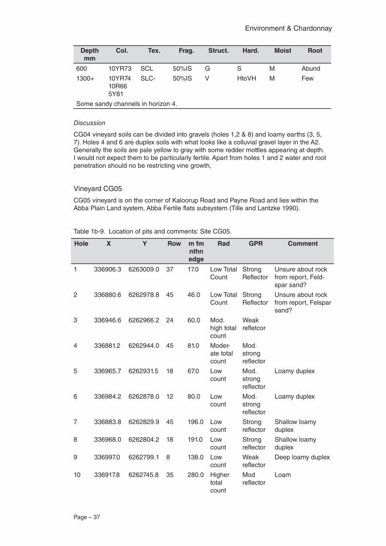
Some sandy channels in horizon 4.
Discussion
CG04 vineyard soils can be divided into gravels (holes 1,2 & 8) and loamy earths (3, 5, 7). Holes 4 and 6 are duplex soils with what looks like a colluvial gravel layer in the A2. Generally the soils are pale yellow to gray with some redder mottles appearing at depth. I would not expect them to be particularly fertile. Apart from holes 1 and 2 water and root penetration should no be restricting vine growth,
Vineyard CG05
CG05 vineyard is on the corner of Kaloorup Road and Payne Road and lies within the Abba Plain Land system, Abba Fertile flats subsystem (Tille and Lantzke 1990).
Table 1b-9. Location of pits and comments: Site CG05.
Hole X Y Row m fm nthn edge
Rad GPR Comment
1 336906.3 6263009.0 37 17.0 Low Total Count
Strong Reflector
Unsure about rock from report, Feld-spar sand?
2 336880.6 6262978.8 45 46.0 Low Total Count
Strong Reflector
Unsure about rock from report, Felspar sand?
3 336946.6 6262966.2 24 60.0 Mod. high total count
Weak refletcor
4 336881.2 6262944.0 45 81.0 Moder-ate total count
Mod. strong reflector
5 336965.7 6262931.5 18 67.0 Low count
Mod. strong reflector
Loamy duplex
6 336984.2 6262878.0 12 80.0 Low count
Mod. strong reflector
Loamy duplex
7 336883.8 6262829.9 45 196.0 Low count
Strong reflector
Shallow loamy duplex
8 336968.0 6262804.2 18 191.0 Low count
Strong reflector
Shallow loamy duplex
9 336997.0 6262799.1 8 138.0 Low count
Weak reflector
Deep loamy duplex
10 336917.8 6262745.8 35 280.0 Higher total count
Mod reflector
Loam
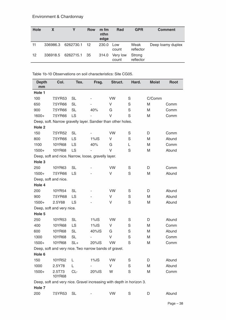
Environment & Chardonnay
Page – 38
Hole X Y Row m fm nthn edge
Rad GPR Comment
11 336986.3 6262730.1 12 230.0 Low count
Weak reflector
Deep loamy duplex
12 336918.5 6262715.1 35 314.0 Very low count
Strong reflector
Table 1b-10 Observations on soil characteristics: Site CG05.
Depth mm
Col. Tex. Frag. Struct. Hard. Moist Root
Hole 1
100 7.5YR53 SL - VW S C/Comm
650 7.5YR66 SL - V S M Comm
900 7.5YR66 SL 40% G S M Comm
1600+ 7.5YR66 LS - V S M Comm
Deep, soft. Narrow gravelly layer. Sandier than other holes.
Hole 2
150 7.5YR52 SL - VW S D Comm
800 7.5YR66 LS 1%IS V S M Abund
1100 10YR68 LS 40% G L M Comm
1500+ 10YR68 LS - V S M Abund
Deep, soft and nice. Narrow, loose, gravelly layer.
Hole 3
250 10YR63 SL - VW S D Comm
1500+ 7.5YR66 LS - V S M Abund
Deep, soft and nice.
Hole 4
200 10YR54 SL - VW S D Abund
900 7.5YR68 LS - V S M Abund
1500+ 2.5Y68 LS - V S M Abund
Deep, soft and very nice.
Hole 5
250 10YR53 SL 1%IS VW S D Abund
400 10YR68 LS 1%IS V S M Comm
600 10YR68 SL 40%IS G S M Abund
1300 10YR68 SL - V S M Comm
1500+ 10YR68 SL+ 20%IS VW S M Comm
Deep, soft and very nice. Two narrow bands of gravel.
Hole 6
150 10YR52 L 1%IS VW S D Abund
1000 2.5Y78 L - V S M Abund
1500+ 2.5T73 10YR68
CL- 20%IS W S M Comm
Deep, soft and very nice. Gravel increasing with depth in horizon 3.
Hole 7
200 7.5YR53 SL - VW S D Abund
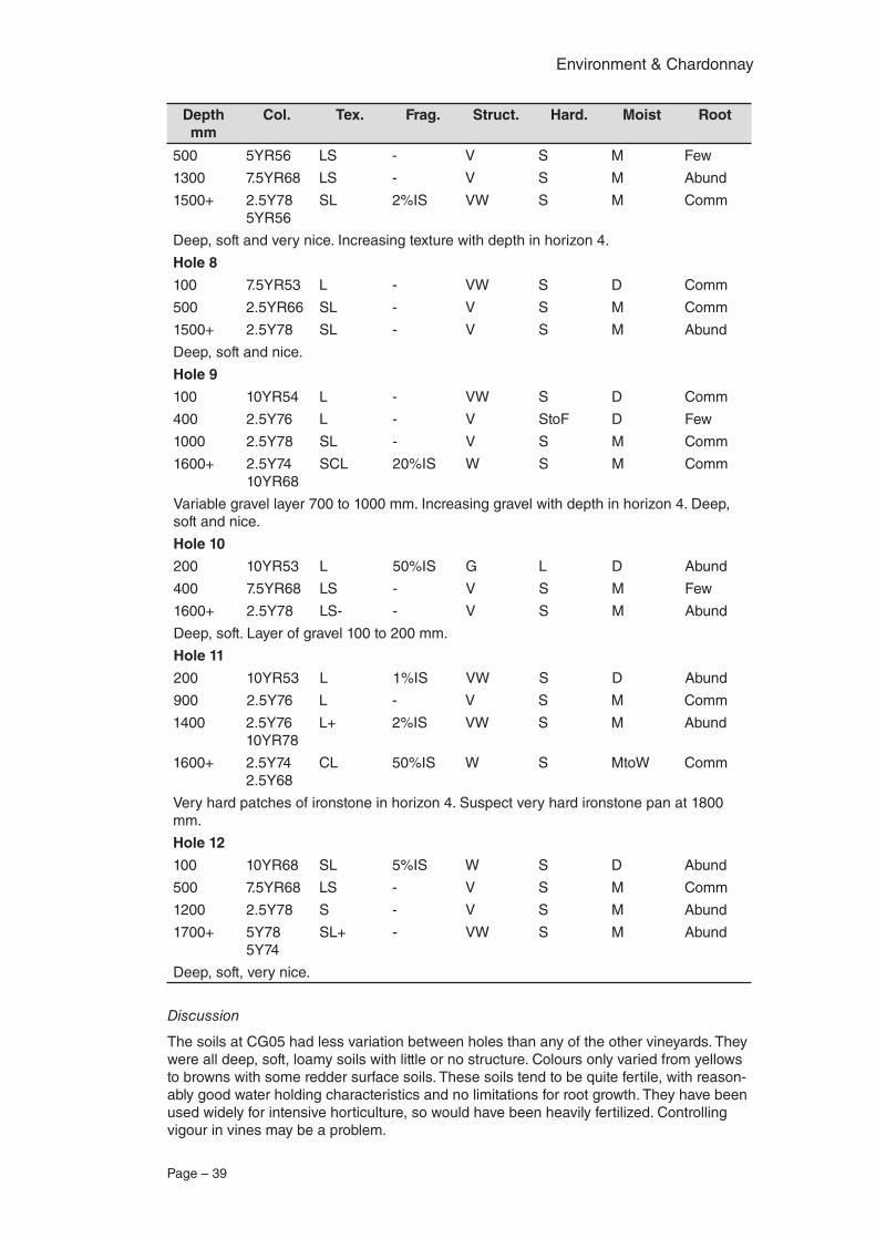
Page – 39
Environment & Chardonnay
Depth mm
Col. Tex. Frag. Struct. Hard. Moist Root
500 5YR56 LS - V S M Few
1300 7.5YR68 LS - V S M Abund
1500+ 2.5Y78 5YR56
SL 2%IS VW S M Comm
Deep, soft and very nice. Increasing texture with depth in horizon 4.
Hole 8
100 7.5YR53 L - VW S D Comm
500 2.5YR66 SL - V S M Comm
1500+ 2.5Y78 SL - V S M Abund
Deep, soft and nice.
Hole 9
100 10YR54 L - VW S D Comm
400 2.5Y76 L - V StoF D Few
1000 2.5Y78 SL - V S M Comm
1600+ 2.5Y74 10YR68
SCL 20%IS W S M Comm
Variable gravel layer 700 to 1000 mm. Increasing gravel with depth in horizon 4. Deep, soft and nice.
Hole 10
200 10YR53 L 50%IS G L D Abund
400 7.5YR68 LS - V S M Few
1600+ 2.5Y78 LS- - V S M Abund
Deep, soft. Layer of gravel 100 to 200 mm.
Hole 11
200 10YR53 L 1%IS VW S D Abund
900 2.5Y76 L - V S M Comm
1400 2.5Y76 10YR78
L+ 2%IS VW S M Abund
1600+ 2.5Y74 2.5Y68
CL 50%IS W S MtoW Comm
Very hard patches of ironstone in horizon 4. Suspect very hard ironstone pan at 1800 mm.
Hole 12
100 10YR68 SL 5%IS W S D Abund
500 7.5YR68 LS - V S M Comm
1200 2.5Y78 S - V S M Abund
1700+ 5Y78 5Y74
SL+ - VW S M Abund
Deep, soft, very nice.
Discussion
The soils at CG05 had less variation between holes than any of the other vineyards. They were all deep, soft, loamy soils with little or no structure. Colours only varied from yellows to browns with some redder surface soils. These soils tend to be quite fertile, with reason-ably good water holding characteristics and no limitations for root growth. They have been used widely for intensive horticulture, so would have been heavily fertilized. Controlling vigour in vines may be a problem.
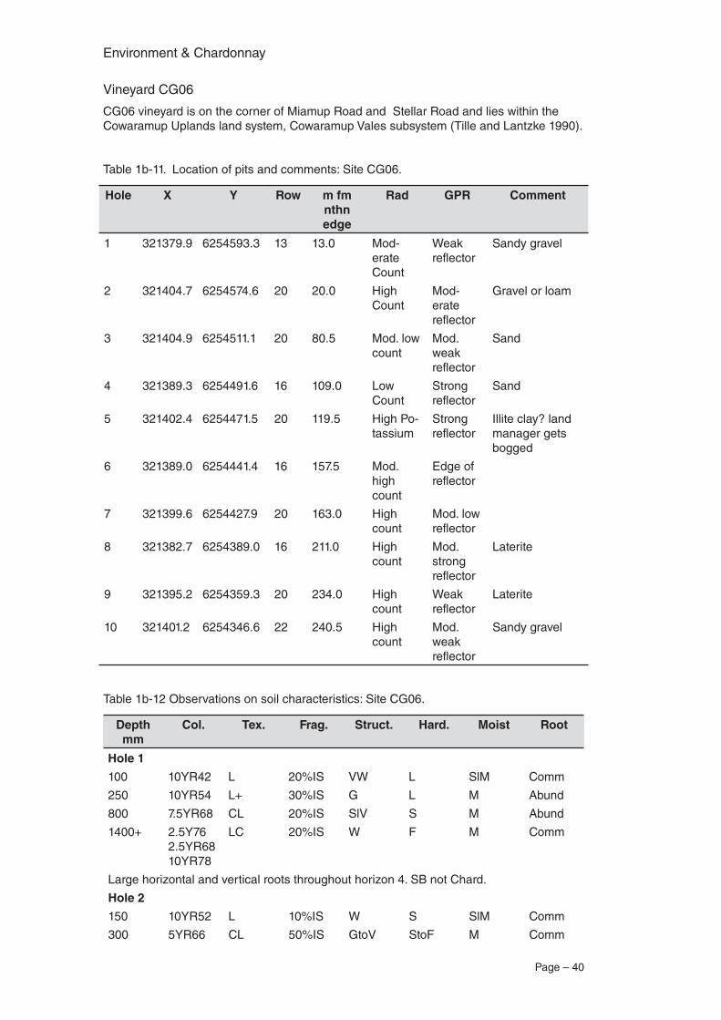
Environment & Chardonnay
Page – 40
Vineyard CG06
CG06 vineyard is on the corner of Miamup Road and Stellar Road and lies within the Cowaramup Uplands land system, Cowaramup Vales subsystem (Tille and Lantzke 1990).
Table 1b-11. Location of pits and comments: Site CG06.
Hole X Y Row m fm nthn edge
Rad GPR Comment
1 321379.9 6254593.3 13 13.0 Mod-erate Count
Weak reflector
Sandy gravel
2 321404.7 6254574.6 20 20.0 High Count
Mod-erate reflector
Gravel or loam
3 321404.9 6254511.1 20 80.5 Mod. low count
Mod. weak reflector
Sand
4 321389.3 6254491.6 16 109.0 Low Count
Strong reflector
Sand
5 321402.4 6254471.5 20 119.5 High Po-tassium
Strong reflector
Illite clay? land manager gets bogged
6 321389.0 6254441.4 16 157.5 Mod. high count
Edge of reflector
7 321399.6 6254427.9 20 163.0 High count
Mod. low reflector
8 321382.7 6254389.0 16 211.0 High count
Mod. strong reflector
Laterite
9 321395.2 6254359.3 20 234.0 High count
Weak reflector
Laterite
10 321401.2 6254346.6 22 240.5 High count
Mod. weak reflector
Sandy gravel
Table 1b-12 Observations on soil characteristics: Site CG06.
Depth mm
Col. Tex. Frag. Struct. Hard. Moist Root
Hole 1
100 10YR42 L 20%IS VW L SlM Comm
250 10YR54 L+ 30%IS G L M Abund
800 7.5YR68 CL 20%IS SlV S M Abund
1400+ 2.5Y76 2.5YR68 10YR78
LC 20%IS W F M Comm
Large horizontal and vertical roots throughout horizon 4. SB not Chard.
Hole 2
150 10YR52 L 10%IS W S SlM Comm
300 5YR66 CL 50%IS GtoV StoF M Comm
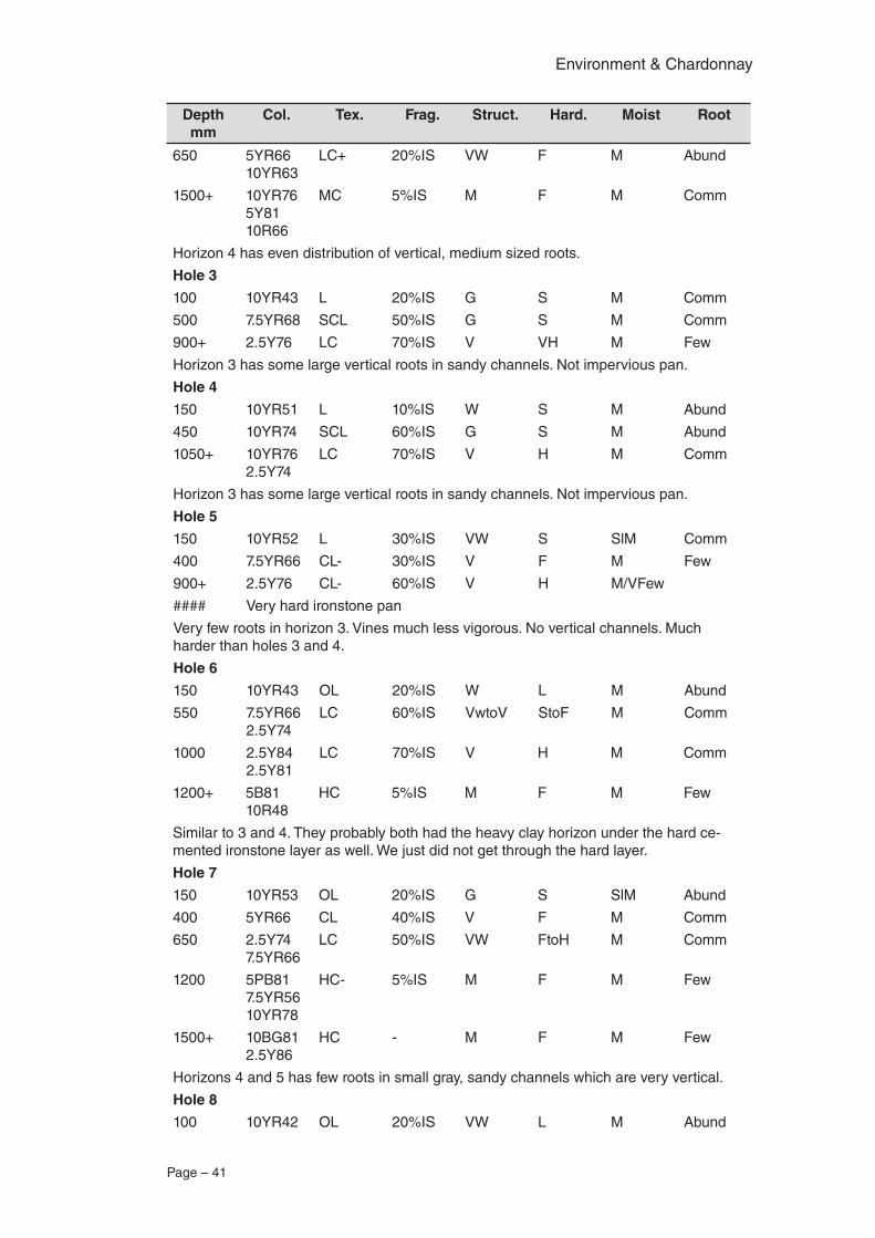
Page – 41
Environment & Chardonnay
Depth mm
Col. Tex. Frag. Struct. Hard. Moist Root
650 5YR66 10YR63
LC+ 20%IS VW F M Abund
1500+ 10YR76 5Y81 10R66
MC 5%IS M F M Comm
Horizon 4 has even distribution of vertical, medium sized roots.
Hole 3
100 10YR43 L 20%IS G S M Comm
500 7.5YR68 SCL 50%IS G S M Comm
900+ 2.5Y76 LC 70%IS V VH M Few
Horizon 3 has some large vertical roots in sandy channels. Not impervious pan.
Hole 4
150 10YR51 L 10%IS W S M Abund
450 10YR74 SCL 60%IS G S M Abund
1050+ 10YR76 2.5Y74
LC 70%IS V H M Comm
Horizon 3 has some large vertical roots in sandy channels. Not impervious pan.
Hole 5
150 10YR52 L 30%IS VW S SlM Comm
400 7.5YR66 CL- 30%IS V F M Few
900+ 2.5Y76 CL- 60%IS V H M/VFew
#### Very hard ironstone pan
Very few roots in horizon 3. Vines much less vigorous. No vertical channels. Much harder than holes 3 and 4.
Hole 6
150 10YR43 OL 20%IS W L M Abund
550 7.5YR66 2.5Y74
LC 60%IS VwtoV StoF M Comm
1000 2.5Y84 2.5Y81
LC 70%IS V H M Comm
1200+ 5B81 10R48
HC 5%IS M F M Few
Similar to 3 and 4. They probably both had the heavy clay horizon under the hard ce-mented ironstone layer as well. We just did not get through the hard layer.
Hole 7
150 10YR53 OL 20%IS G S SlM Abund
400 5YR66 CL 40%IS V F M Comm
650 2.5Y74 7.5YR66
LC 50%IS VW FtoH M Comm
1200 5PB81 7.5YR56 10YR78
HC- 5%IS M F M Few
1500+ 10BG81 2.5Y86
HC - M F M Few
Horizons 4 and 5 has few roots in small gray, sandy channels which are very vertical.
Hole 8
100 10YR42 OL 20%IS VW L M Abund
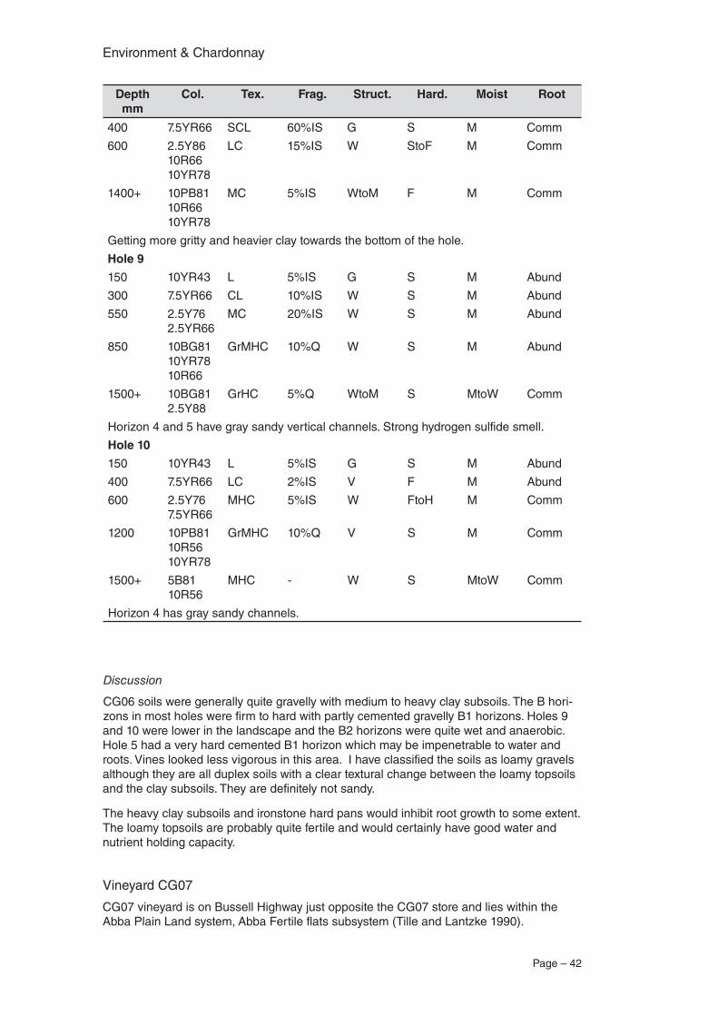
Environment & Chardonnay
Page – 42
Depth mm
Col. Tex. Frag. Struct. Hard. Moist Root
400 7.5YR66 SCL 60%IS G S M Comm
600 2.5Y86 10R66 10YR78
LC 15%IS W StoF M Comm
1400+ 10PB81 10R66 10YR78
MC 5%IS WtoM F M Comm
Getting more gritty and heavier clay towards the bottom of the hole.
Hole 9
150 10YR43 L 5%IS G S M Abund
300 7.5YR66 CL 10%IS W S M Abund
550 2.5Y76 2.5YR66
MC 20%IS W S M Abund
850 10BG81 10YR78 10R66
GrMHC 10%Q W S M Abund
1500+ 10BG81 2.5Y88
GrHC 5%Q WtoM S MtoW Comm
Horizon 4 and 5 have gray sandy vertical channels. Strong hydrogen sulfide smell.
Hole 10
150 10YR43 L 5%IS G S M Abund
400 7.5YR66 LC 2%IS V F M Abund
600 2.5Y76 7.5YR66
MHC 5%IS W FtoH M Comm
1200 10PB81 10R56 10YR78
GrMHC 10%Q V S M Comm
1500+ 5B81 10R56
MHC - W S MtoW Comm
Horizon 4 has gray sandy channels.
Discussion
CG06 soils were generally quite gravelly with medium to heavy clay subsoils. The B hori-zons in most holes were firm to hard with partly cemented gravelly B1 horizons. Holes 9 and 10 were lower in the landscape and the B2 horizons were quite wet and anaerobic. Hole 5 had a very hard cemented B1 horizon which may be impenetrable to water and roots. Vines looked less vigorous in this area. I have classified the soils as loamy gravels although they are all duplex soils with a clear textural change between the loamy topsoils and the clay subsoils. They are definitely not sandy.
The heavy clay subsoils and ironstone hard pans would inhibit root growth to some extent. The loamy topsoils are probably quite fertile and would certainly have good water and nutrient holding capacity.
Vineyard CG07
CG07 vineyard is on Bussell Highway just opposite the CG07 store and lies within the Abba Plain Land system, Abba Fertile flats subsystem (Tille and Lantzke 1990).
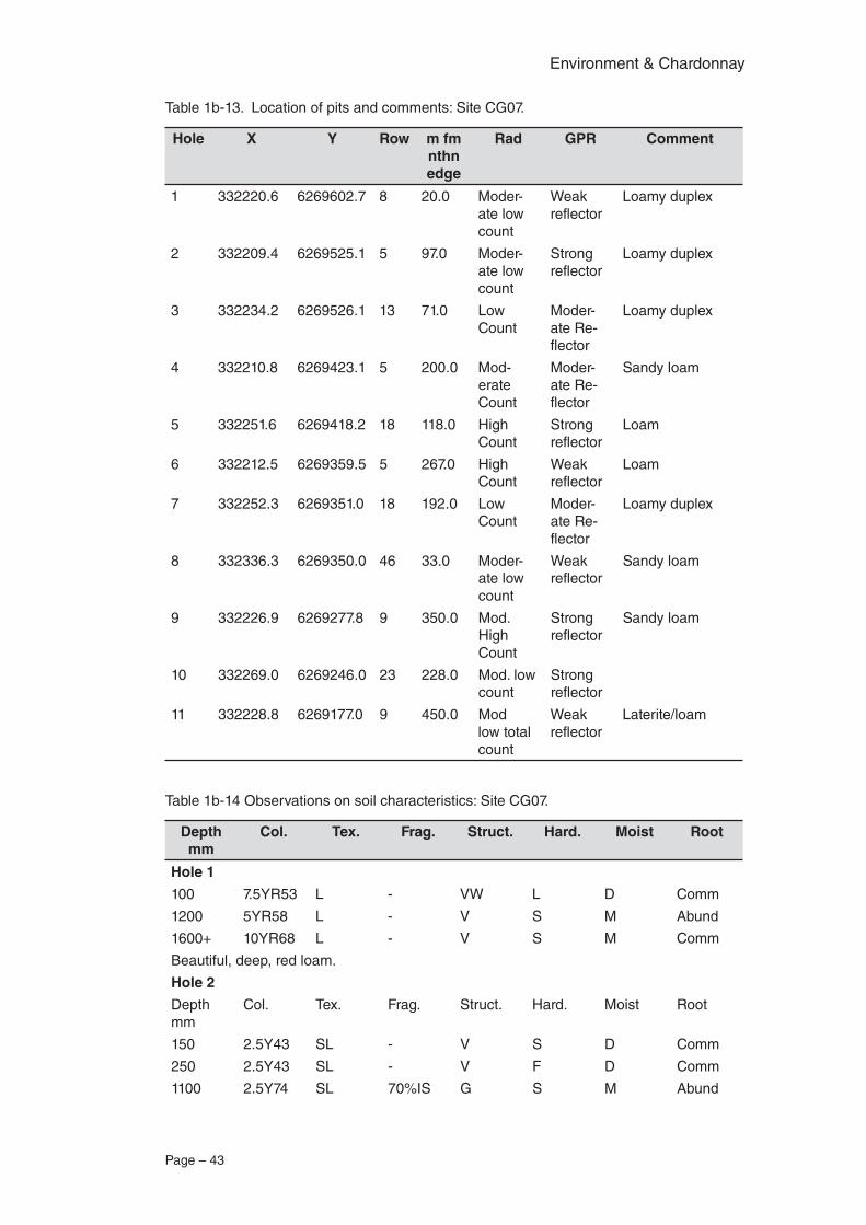
Page – 43
Environment & Chardonnay
Table 1b-13. Location of pits and comments: Site CG07.
Hole X Y Row m fm nthn edge
Rad GPR Comment
1 332220.6 6269602.7 8 20.0 Moder-ate low count
Weak reflector
Loamy duplex
2 332209.4 6269525.1 5 97.0 Moder-ate low count
Strong reflector
Loamy duplex
3 332234.2 6269526.1 13 71.0 Low Count
Moder-ate Re-flector
Loamy duplex
4 332210.8 6269423.1 5 200.0 Mod-erate Count
Moder-ate Re-flector
Sandy loam
5 332251.6 6269418.2 18 118.0 High Count
Strong reflector
Loam
6 332212.5 6269359.5 5 267.0 High Count
Weak reflector
Loam
7 332252.3 6269351.0 18 192.0 Low Count
Moder-ate Re-flector
Loamy duplex
8 332336.3 6269350.0 46 33.0 Moder-ate low count
Weak reflector
Sandy loam
9 332226.9 6269277.8 9 350.0 Mod. High Count
Strong reflector
Sandy loam
10 332269.0 6269246.0 23 228.0 Mod. low count
Strong reflector
11 332228.8 6269177.0 9 450.0 Mod low total count
Weak reflector
Laterite/loam
Table 1b-14 Observations on soil characteristics: Site CG07.
Depth mm
Col. Tex. Frag. Struct. Hard. Moist Root
Hole 1
100 7.5YR53 L - VW L D Comm
1200 5YR58 L - V S M Abund
1600+ 10YR68 L - V S M Comm
Beautiful, deep, red loam.
Hole 2
Depth mm
Col. Tex. Frag. Struct. Hard. Moist Root
150 2.5Y43 SL - V S D Comm
250 2.5Y43 SL - V F D Comm
1100 2.5Y74 SL 70%IS G S M Abund
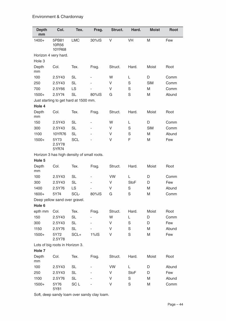
Environment & Chardonnay
Page – 44
Depth mm
Col. Tex. Frag. Struct. Hard. Moist Root
1400+ 5PB81 10R56 10YR68
LMC 30%IS V VH M Few
Horizon 4 very hard.
Hole 3
Depth mm
Col. Tex. Frag. Struct. Hard. Moist Root
100 2.5Y43 SL - W L D Comm
250 2.5Y43 SL - V S SlM Comm
700 2.5Y66 LS - V S M Comm
1500+ 2.5Y74 SL 80%IS G S M Abund
Just starting to get hard at 1500 mm.
Hole 4
Depth mm
Col. Tex. Frag. Struct. Hard. Moist Root
150 2.5Y43 SL - W L D Comm
300 2.5Y43 SL - V S SlM Comm
1100 10YR76 SL - V S M Abund
1500+ 5Y73 2.5Y78 5YR74
SCL - V F M Few
Horizon 3 has high density of small roots.
Hole 5
Depth mm
Col. Tex. Frag. Struct. Hard. Moist Root
100 2.5Y43 SL - VW L D Comm
300 2.5Y43 SL - V StoF D Few
1400 2.5Y76 LS - V S M Abund
1600+ 5Y74 SCL- 80%IS G S M Comm
Deep yellow sand over gravel.
Hole 6
epth mm Col. Tex. Frag. Struct. Hard. Moist Root
150 2.5Y43 SL - W L D Comm
300 2.5Y43 SL - V S D Few
1150 2.5Y76 SL - V S M Abund
1500+ 5Y72 2.5Y78
SCL+ 1%IS V S M Few
Lots of big roots in Horizon 3.
Hole 7
Depth mm
Col. Tex. Frag. Struct. Hard. Moist Root
100 2.5Y43 SL - VW L D Abund
250 2.5Y43 SL - V StoF D Few
1100 2.5Y76 SL - V S M Abund
1500+ 5Y76 5Y81
SC L - V S M Comm
Soft, deep sandy loam over sandy clay loam.
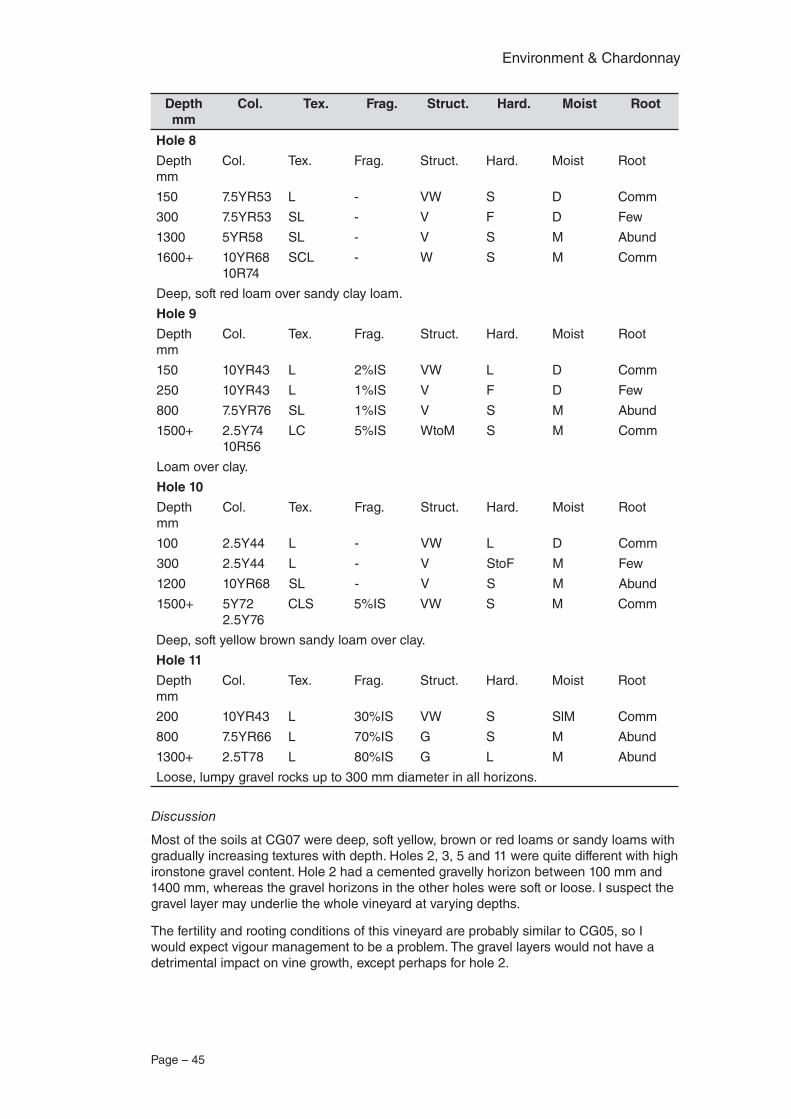
Page – 45
Environment & Chardonnay
Depth mm
Col. Tex. Frag. Struct. Hard. Moist Root
Hole 8
Depth mm
Col. Tex. Frag. Struct. Hard. Moist Root
150 7.5YR53 L - VW S D Comm
300 7.5YR53 SL - V F D Few
1300 5YR58 SL - V S M Abund
1600+ 10YR68 10R74
SCL - W S M Comm
Deep, soft red loam over sandy clay loam.
Hole 9
Depth mm
Col. Tex. Frag. Struct. Hard. Moist Root
150 10YR43 L 2%IS VW L D Comm
250 10YR43 L 1%IS V F D Few
800 7.5YR76 SL 1%IS V S M Abund
1500+ 2.5Y74 10R56
LC 5%IS WtoM S M Comm
Loam over clay.
Hole 10
Depth mm
Col. Tex. Frag. Struct. Hard. Moist Root
100 2.5Y44 L - VW L D Comm
300 2.5Y44 L - V StoF M Few
1200 10YR68 SL - V S M Abund
1500+ 5Y72 2.5Y76
CLS 5%IS VW S M Comm
Deep, soft yellow brown sandy loam over clay.
Hole 11
Depth mm
Col. Tex. Frag. Struct. Hard. Moist Root
200 10YR43 L 30%IS VW S SlM Comm
800 7.5YR66 L 70%IS G S M Abund
1300+ 2.5T78 L 80%IS G L M Abund
Loose, lumpy gravel rocks up to 300 mm diameter in all horizons.
Discussion
Most of the soils at CG07 were deep, soft yellow, brown or red loams or sandy loams with gradually increasing textures with depth. Holes 2, 3, 5 and 11 were quite different with high ironstone gravel content. Hole 2 had a cemented gravelly horizon between 100 mm and 1400 mm, whereas the gravel horizons in the other holes were soft or loose. I suspect the gravel layer may underlie the whole vineyard at varying depths.
The fertility and rooting conditions of this vineyard are probably similar to CG05, so I would expect vigour management to be a problem. The gravel layers would not have a detrimental impact on vine growth, except perhaps for hole 2.
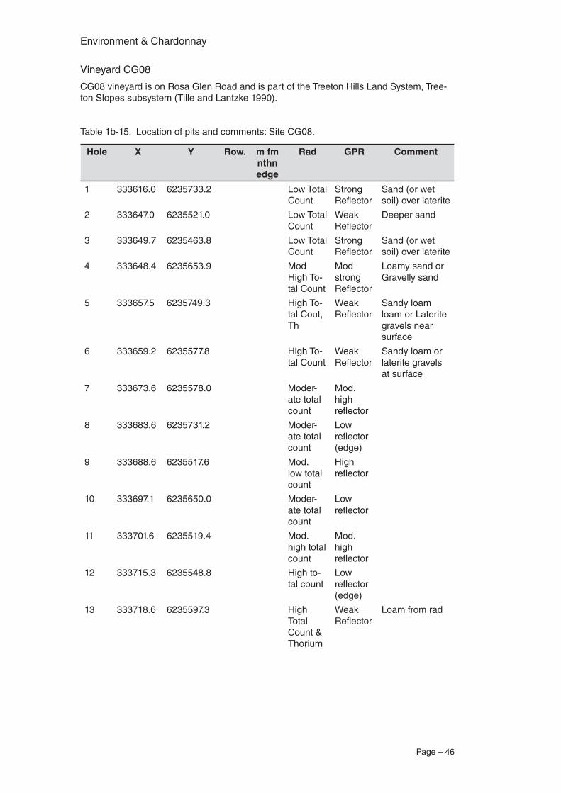
Environment & Chardonnay
Page – 46
Vineyard CG08
CG08 vineyard is on Rosa Glen Road and is part of the Treeton Hills Land System, Tree-ton Slopes subsystem (Tille and Lantzke 1990).
Table 1b-15. Location of pits and comments: Site CG08.
Hole X Y Row. m fm nthn edge
Rad GPR Comment
1 333616.0 6235733.2 Low Total Count
Strong Reflector
Sand (or wet soil) over laterite
2 333647.0 6235521.0 Low Total Count
Weak Reflector
Deeper sand
3 333649.7 6235463.8 Low Total Count
Strong Reflector
Sand (or wet soil) over laterite
4 333648.4 6235653.9 Mod High To-tal Count
Mod strong Reflector
Loamy sand or Gravelly sand
5 333657.5 6235749.3 High To-tal Cout, Th
Weak Reflector
Sandy loam loam or Laterite gravels near surface
6 333659.2 6235577.8 High To-tal Count
Weak Reflector
Sandy loam or laterite gravels at surface
7 333673.6 6235578.0 Moder-ate total count
Mod. high reflector
8 333683.6 6235731.2 Moder-ate total count
Low reflector (edge)
9 333688.6 6235517.6 Mod. low total count
High reflector
10 333697.1 6235650.0 Moder-ate total count
Low reflector
11 333701.6 6235519.4 Mod. high total count
Mod. high reflector
12 333715.3 6235548.8 High to-tal count
Low reflector (edge)
13 333718.6 6235597.3 High Total Count & Thorium
Weak Reflector
Loam from rad
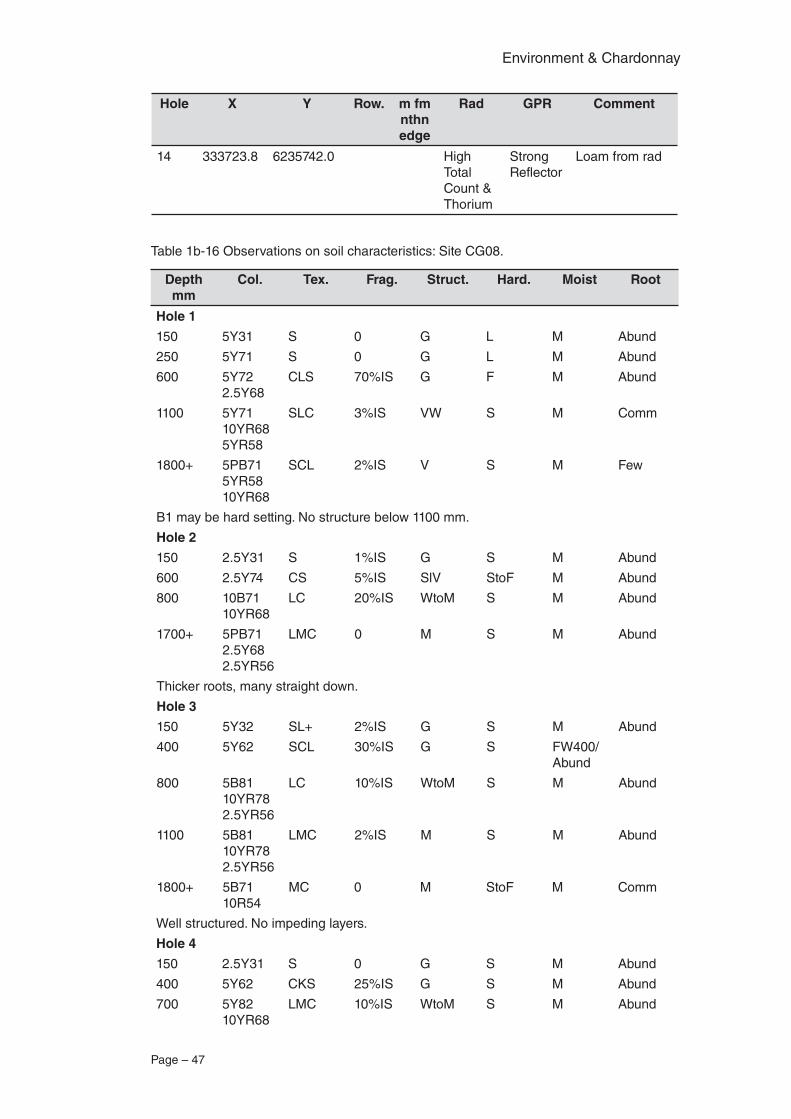
Page – 47
Environment & Chardonnay
Hole X Y Row. m fm nthn edge
Rad GPR Comment
14 333723.8 6235742.0 High Total Count & Thorium
Strong Reflector
Loam from rad
Table 1b-16 Observations on soil characteristics: Site CG08.
Depth mm
Col. Tex. Frag. Struct. Hard. Moist Root
Hole 1
150 5Y31 S 0 G L M Abund
250 5Y71 S 0 G L M Abund
600 5Y72 2.5Y68
CLS 70%IS G F M Abund
1100 5Y71 10YR68 5YR58
SLC 3%IS VW S M Comm
1800+ 5PB71 5YR58 10YR68
SCL 2%IS V S M Few
B1 may be hard setting. No structure below 1100 mm.
Hole 2
150 2.5Y31 S 1%IS G S M Abund
600 2.5Y74 CS 5%IS SlV StoF M Abund
800 10B71 10YR68
LC 20%IS WtoM S M Abund
1700+ 5PB71 2.5Y68 2.5YR56
LMC 0 M S M Abund
Thicker roots, many straight down.
Hole 3
150 5Y32 SL+ 2%IS G S M Abund
400 5Y62 SCL 30%IS G S FW400/Abund
800 5B81 10YR78 2.5YR56
LC 10%IS WtoM S M Abund
1100 5B81 10YR78 2.5YR56
LMC 2%IS M S M Abund
1800+ 5B71 10R54
MC 0 M StoF M Comm
Well structured. No impeding layers.
Hole 4
150 2.5Y31 S 0 G S M Abund
400 5Y62 CKS 25%IS G S M Abund
700 5Y82 10YR68
LMC 10%IS WtoM S M Abund
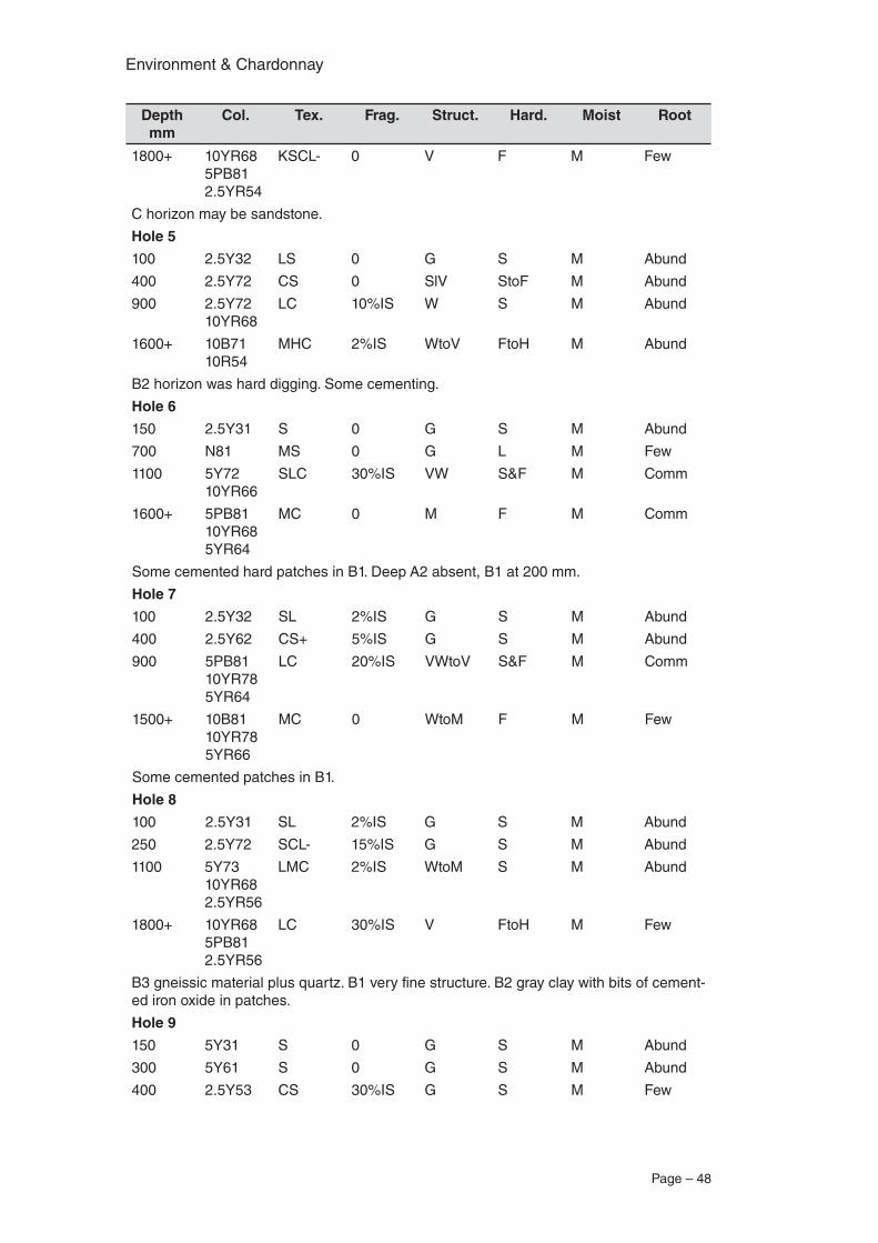
Environment & Chardonnay
Page – 48
Depth mm
Col. Tex. Frag. Struct. Hard. Moist Root
1800+ 10YR68 5PB81 2.5YR54
KSCL- 0 V F M Few
C horizon may be sandstone.
Hole 5
100 2.5Y32 LS 0 G S M Abund
400 2.5Y72 CS 0 SlV StoF M Abund
900 2.5Y72 10YR68
LC 10%IS W S M Abund
1600+ 10B71 10R54
MHC 2%IS WtoV FtoH M Abund
B2 horizon was hard digging. Some cementing.
Hole 6
150 2.5Y31 S 0 G S M Abund
700 N81 MS 0 G L M Few
1100 5Y72 10YR66
SLC 30%IS VW S&F M Comm
1600+ 5PB81 10YR68 5YR64
MC 0 M F M Comm
Some cemented hard patches in B1. Deep A2 absent, B1 at 200 mm.
Hole 7
100 2.5Y32 SL 2%IS G S M Abund
400 2.5Y62 CS+ 5%IS G S M Abund
900 5PB81 10YR78 5YR64
LC 20%IS VWtoV S&F M Comm
1500+ 10B81 10YR78 5YR66
MC 0 WtoM F M Few
Some cemented patches in B1.
Hole 8
100 2.5Y31 SL 2%IS G S M Abund
250 2.5Y72 SCL- 15%IS G S M Abund
1100 5Y73 10YR68 2.5YR56
LMC 2%IS WtoM S M Abund
1800+ 10YR68 5PB81 2.5YR56
LC 30%IS V FtoH M Few
B3 gneissic material plus quartz. B1 very fine structure. B2 gray clay with bits of cement-ed iron oxide in patches.
Hole 9
150 5Y31 S 0 G S M Abund
300 5Y61 S 0 G S M Abund
400 2.5Y53 CS 30%IS G S M Few
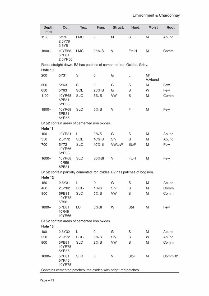
Page – 49
Environment & Chardonnay
Depth mm
Col. Tex. Frag. Struct. Hard. Moist Root
1100 5Y74 2.5Y78 2.5Y51
LMC 0 M S M Abund
1800+ 10YR68 5PB81 2.5YR56
LMC 25%IS V Fto H M Comm
Roots straight down. B2 has patches of cemented Iron Oxides. Gritty.
Hole 10
200 5Y31 S 0 G L M/V.Abund
500 5Y63 S 0 G S M Few
650 5Y63 SCL 20%IS G S W Few
1100 10YR68 5PB81 5YR56
SLC 5%IS VW S M Comm
1800+ 10YR68 5PB81 5YR56
SLC 5%IS V F M Few
B1&2 contain areas of cemented iron oxides.
Hole 11
150 10YR31 L 2%IS G S M Abund
350 2.5Y72 SCL 10%IS SlV S M Abund
700 5Y72 10YR66 5YR56
SLC 10%IS VWtoW StoF M Few
1600+ 10YR68 10R56 5PB81
SLC 30%BI V FtoH M Few
B1&2 contain partially cemented iron oxides. B2 has patches of bog iron.
Hole 12
150 2.5Y31 L 0 G S M Abund
400 2.5Y62 SCL- 1%IS SlV S M Comm
800 5PB81 10YR78 5R56
SLC 5%IS VW S M Comm
1600+ 5PB81 10R46 10YR66
LC 5%BI W S&F M Few
B1&2 contain areas of cemented iron oxides.
Hole 13
100 2.5Y32 L 0 G S M Abund
550 2.5Y72 SCL- 5%IS SlV S W Abund
800 5PB81 10YR78 5YR56
SLC 2%IS VW S M Comm
1600+ 5PB81 5YR46 10YR78
SLC 0 V StoF M CommB2
Contains cemented patches iron oxides with bright red patches.
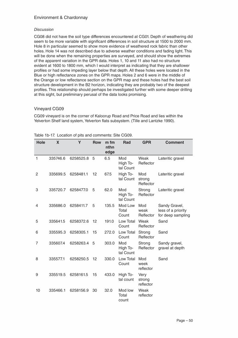
Environment & Chardonnay
Page – 50
Discussion
CG08 did not have the soil type differences encountered at CG01. Depth of weathering did seem to be more variable with significant differences in soil structure at 1500 to 2000 mm. Hole 8 in particular seemed to show more evidence of weathered rock fabric than other holes. Hole 14 was not described due to adverse weather conditions and fading light. This will be done when the remaining properties are surveyed, and should show the extremes of the apparent variation in the GPR data. Holes 1, 10 and 11 also had no structure evident at 1600 to 1800 mm, which I would interpret as indicating that they are shallower profiles or had some impeding layer below that depth. All these holes were located in the Blue or high reflectance zones on the GPR maps. Holes 2 and 6 were in the middle of the Orange or low reflectance section on the GPR map and these holes had the best soil structure development in the B2 horizon, indicating they are probably two of the deepest profiles. This relationship should perhaps be investigated further with some deeper drilling at this sight, but preliminary perusal of the data looks promising.
Vineyard CG09
CG09 vineyard is on the corner of Kaloorup Road and Price Road and lies within the Yelverton Shelf land system, Yelverton flats subsystem. (Tille and Lantzke 1990).
Table 1b-17. Location of pits and comments: Site CG09.
Hole X Y Row m fm nthn edge
Rad GPR Comment
1 335746.6 6258525.8 5 6.5 Mod High To-tal Count
Weak Reflector
Lateritic gravel
2 335699.5 6258481.1 12 67.5 High To-tal Count
Mod strong Reflector
Lateritic gravel
3 335720.7 6258477.0 5 62.0 Mod High To-tal Count
Strong Reflector
Lateritic gravel
4 335686.0 6258411.7 5 135.5 Mod Low Total Count
Mod weak Reflector
Sandy Gravel, less of a priority for deep sampling
5 335641.5 6258372.6 12 191.0 Low Total Count
Weak Reflector
Sand
6 335595.3 6258305.1 15 272.0 Low Total Count
Strong Reflector
Sand
7 335607.4 6258263.4 5 303.0 Mod High To-tal Count
Strong Reflector
Sandy gravel, gravel at depth
8 335577.1 6258250.5 12 330.0 Low Total Count
Mod week reflector
Sand
9 335519.5 6258161.5 15 433.0 High To-tal count
Very strong reflector
10 335466.1 6258156.9 30 32.0 Mod low Total count
Weak reflector
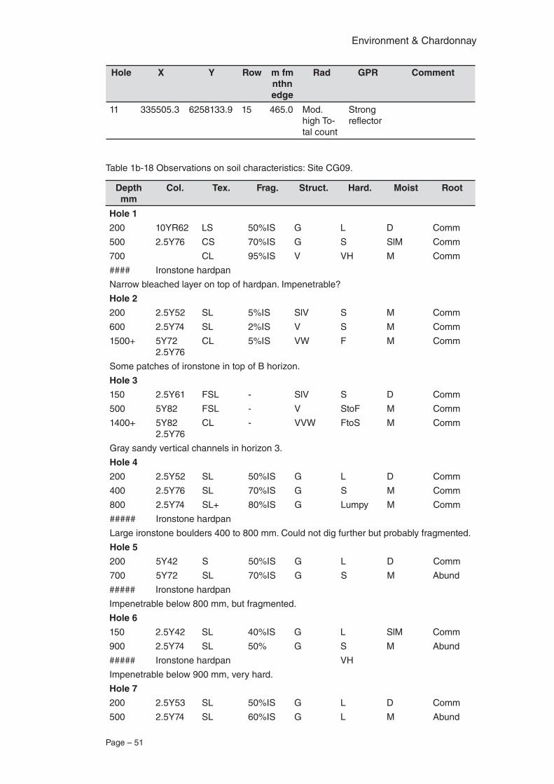
Page – 51
Environment & Chardonnay
Hole X Y Row m fm nthn edge
Rad GPR Comment
11 335505.3 6258133.9 15 465.0 Mod. high To-tal count
Strong reflector
Table 1b-18 Observations on soil characteristics: Site CG09.
Depth mm
Col. Tex. Frag. Struct. Hard. Moist Root
Hole 1
200 10YR62 LS 50%IS G L D Comm
500 2.5Y76 CS 70%IS G S SlM Comm
700 CL 95%IS V VH M Comm
#### Ironstone hardpan
Narrow bleached layer on top of hardpan. Impenetrable?
Hole 2
200 2.5Y52 SL 5%IS SlV S M Comm
600 2.5Y74 SL 2%IS V S M Comm
1500+ 5Y72 2.5Y76
CL 5%IS VW F M Comm
Some patches of ironstone in top of B horizon.
Hole 3
150 2.5Y61 FSL - SlV S D Comm
500 5Y82 FSL - V StoF M Comm
1400+ 5Y82 2.5Y76
CL - VVW FtoS M Comm
Gray sandy vertical channels in horizon 3.
Hole 4
200 2.5Y52 SL 50%IS G L D Comm
400 2.5Y76 SL 70%IS G S M Comm
800 2.5Y74 SL+ 80%IS G Lumpy M Comm
##### Ironstone hardpan
Large ironstone boulders 400 to 800 mm. Could not dig further but probably fragmented.
Hole 5
200 5Y42 S 50%IS G L D Comm
700 5Y72 SL 70%IS G S M Abund
##### Ironstone hardpan
Impenetrable below 800 mm, but fragmented.
Hole 6
150 2.5Y42 SL 40%IS G L SlM Comm
900 2.5Y74 SL 50% G S M Abund
##### Ironstone hardpan VH
Impenetrable below 900 mm, very hard.
Hole 7
200 2.5Y53 SL 50%IS G L D Comm
500 2.5Y74 SL 60%IS G L M Abund
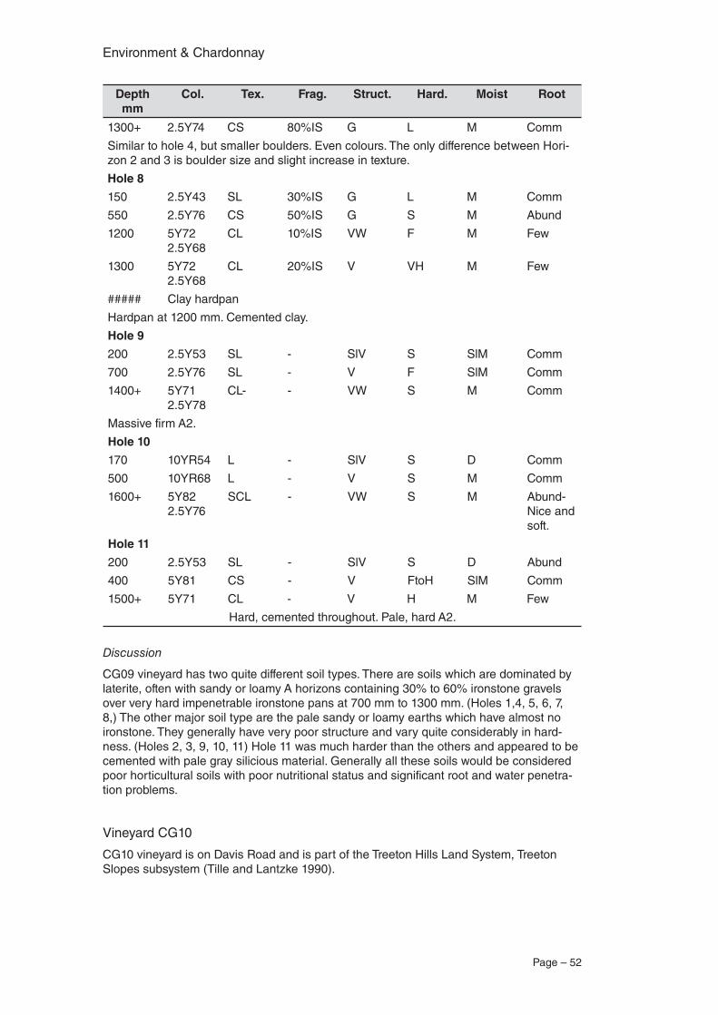
Environment & Chardonnay
Page – 52
Depth mm
Col. Tex. Frag. Struct. Hard. Moist Root
1300+ 2.5Y74 CS 80%IS G L M Comm
Similar to hole 4, but smaller boulders. Even colours. The only difference between Hori-zon 2 and 3 is boulder size and slight increase in texture.
Hole 8
150 2.5Y43 SL 30%IS G L M Comm
550 2.5Y76 CS 50%IS G S M Abund
1200 5Y72 2.5Y68
CL 10%IS VW F M Few
1300 5Y72 2.5Y68
CL 20%IS V VH M Few
##### Clay hardpan
Hardpan at 1200 mm. Cemented clay.
Hole 9
200 2.5Y53 SL - SlV S SlM Comm
700 2.5Y76 SL - V F SlM Comm
1400+ 5Y71 2.5Y78
CL- - VW S M Comm
Massive firm A2.
Hole 10
170 10YR54 L - SlV S D Comm
500 10YR68 L - V S M Comm
1600+ 5Y82 2.5Y76
SCL - VW S M Abund-Nice and soft.
Hole 11
200 2.5Y53 SL - SlV S D Abund
400 5Y81 CS - V FtoH SlM Comm
1500+ 5Y71 CL - V H M Few
Hard, cemented throughout. Pale, hard A2.
Discussion
CG09 vineyard has two quite different soil types. There are soils which are dominated by laterite, often with sandy or loamy A horizons containing 30% to 60% ironstone gravels over very hard impenetrable ironstone pans at 700 mm to 1300 mm. (Holes 1,4, 5, 6, 7, 8,) The other major soil type are the pale sandy or loamy earths which have almost no ironstone. They generally have very poor structure and vary quite considerably in hard-ness. (Holes 2, 3, 9, 10, 11) Hole 11 was much harder than the others and appeared to be cemented with pale gray silicious material. Generally all these soils would be considered poor horticultural soils with poor nutritional status and significant root and water penetra-tion problems.
Vineyard CG10
CG10 vineyard is on Davis Road and is part of the Treeton Hills Land System, Treeton Slopes subsystem (Tille and Lantzke 1990).
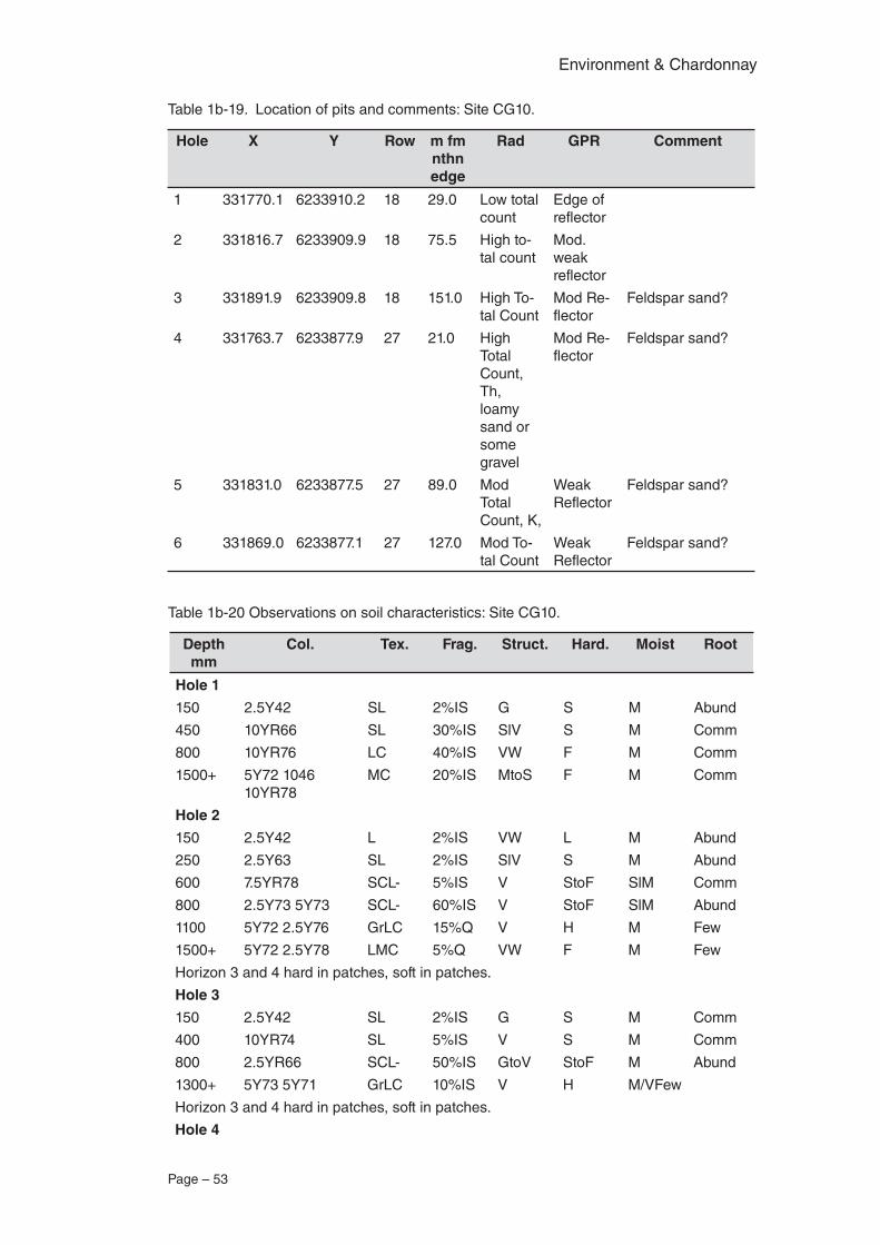
Page – 53
Environment & Chardonnay
Table 1b-19. Location of pits and comments: Site CG10.
Hole X Y Row m fm nthn edge
Rad GPR Comment
1 331770.1 6233910.2 18 29.0 Low total count
Edge of reflector
2 331816.7 6233909.9 18 75.5 High to-tal count
Mod. weak reflector
3 331891.9 6233909.8 18 151.0 High To-tal Count
Mod Re-flector
Feldspar sand?
4 331763.7 6233877.9 27 21.0 High Total Count, Th, loamy sand or some gravel
Mod Re-flector
Feldspar sand?
5 331831.0 6233877.5 27 89.0 Mod Total Count, K,
Weak Reflector
Feldspar sand?
6 331869.0 6233877.1 27 127.0 Mod To-tal Count
Weak Reflector
Feldspar sand?
Table 1b-20 Observations on soil characteristics: Site CG10.
Depth mm
Col. Tex. Frag. Struct. Hard. Moist Root
Hole 1
150 2.5Y42 SL 2%IS G S M Abund
450 10YR66 SL 30%IS SlV S M Comm
800 10YR76 LC 40%IS VW F M Comm
1500+ 5Y72 1046 10YR78
MC 20%IS MtoS F M Comm
Hole 2
150 2.5Y42 L 2%IS VW L M Abund
250 2.5Y63 SL 2%IS SlV S M Abund
600 7.5YR78 SCL- 5%IS V StoF SlM Comm
800 2.5Y73 5Y73 SCL- 60%IS V StoF SlM Abund
1100 5Y72 2.5Y76 GrLC 15%Q V H M Few
1500+ 5Y72 2.5Y78 LMC 5%Q VW F M Few
Horizon 3 and 4 hard in patches, soft in patches.
Hole 3
150 2.5Y42 SL 2%IS G S M Comm
400 10YR74 SL 5%IS V S M Comm
800 2.5YR66 SCL- 50%IS GtoV StoF M Abund
1300+ 5Y73 5Y71 GrLC 10%IS V H M/VFew
Horizon 3 and 4 hard in patches, soft in patches.
Hole 4
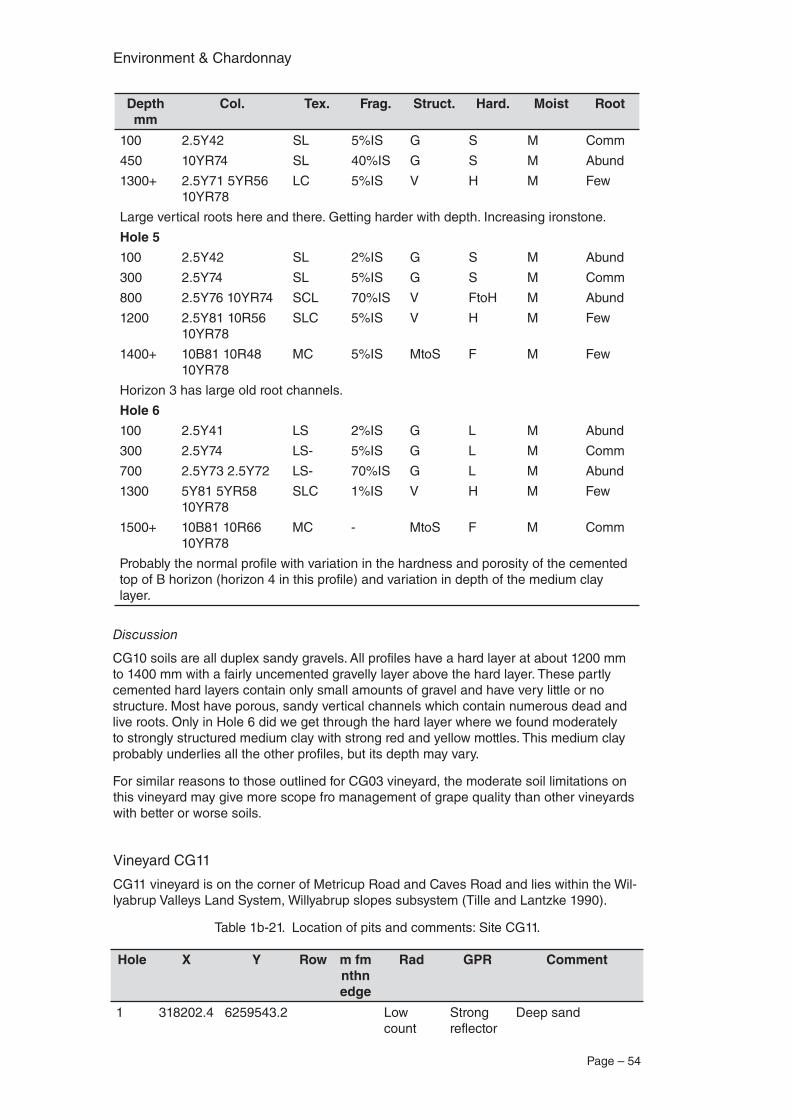
Environment & Chardonnay
Page – 54
Depth mm
Col. Tex. Frag. Struct. Hard. Moist Root
100 2.5Y42 SL 5%IS G S M Comm
450 10YR74 SL 40%IS G S M Abund
1300+ 2.5Y71 5YR56 10YR78
LC 5%IS V H M Few
Large vertical roots here and there. Getting harder with depth. Increasing ironstone.
Hole 5
100 2.5Y42 SL 2%IS G S M Abund
300 2.5Y74 SL 5%IS G S M Comm
800 2.5Y76 10YR74 SCL 70%IS V FtoH M Abund
1200 2.5Y81 10R56 10YR78
SLC 5%IS V H M Few
1400+ 10B81 10R48 10YR78
MC 5%IS MtoS F M Few
Horizon 3 has large old root channels.
Hole 6
100 2.5Y41 LS 2%IS G L M Abund
300 2.5Y74 LS- 5%IS G L M Comm
700 2.5Y73 2.5Y72 LS- 70%IS G L M Abund
1300 5Y81 5YR58 10YR78
SLC 1%IS V H M Few
1500+ 10B81 10R66 10YR78
MC - MtoS F M Comm
Probably the normal profile with variation in the hardness and porosity of the cemented top of B horizon (horizon 4 in this profile) and variation in depth of the medium clay layer.
Discussion
CG10 soils are all duplex sandy gravels. All profiles have a hard layer at about 1200 mm to 1400 mm with a fairly uncemented gravelly layer above the hard layer. These partly cemented hard layers contain only small amounts of gravel and have very little or no structure. Most have porous, sandy vertical channels which contain numerous dead and live roots. Only in Hole 6 did we get through the hard layer where we found moderately to strongly structured medium clay with strong red and yellow mottles. This medium clay probably underlies all the other profiles, but its depth may vary.
For similar reasons to those outlined for CG03 vineyard, the moderate soil limitations on this vineyard may give more scope fro management of grape quality than other vineyards with better or worse soils.
Vineyard CG11
CG11 vineyard is on the corner of Metricup Road and Caves Road and lies within the Wil-lyabrup Valleys Land System, Willyabrup slopes subsystem (Tille and Lantzke 1990).
Table 1b-21. Location of pits and comments: Site CG11.
Hole X Y Row m fm nthn edge
Rad GPR Comment
1 318202.4 6259543.2 Low count
Strong reflector
Deep sand
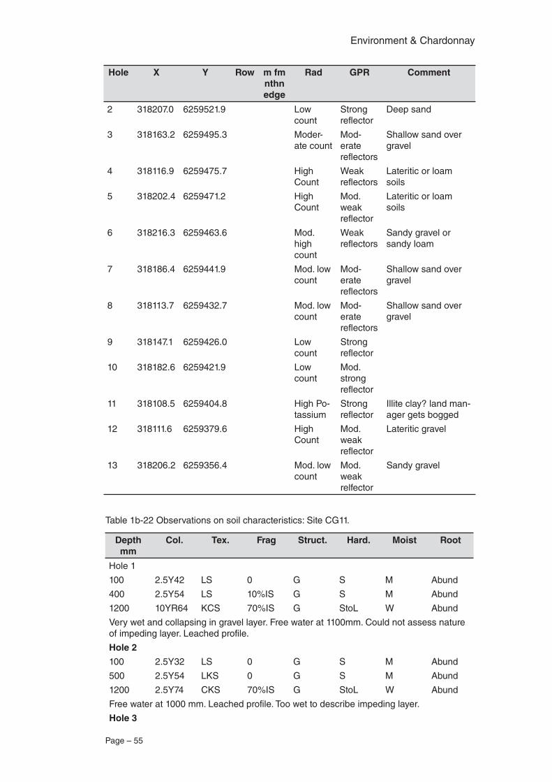
Page – 55
Environment & Chardonnay
Hole X Y Row m fm nthn edge
Rad GPR Comment
2 318207.0 6259521.9 Low count
Strong reflector
Deep sand
3 318163.2 6259495.3 Moder-ate count
Mod-erate reflectors
Shallow sand over gravel
4 318116.9 6259475.7 High Count
Weak reflectors
Lateritic or loam soils
5 318202.4 6259471.2 High Count
Mod. weak reflector
Lateritic or loam soils
6 318216.3 6259463.6 Mod. high count
Weak reflectors
Sandy gravel or sandy loam
7 318186.4 6259441.9 Mod. low count
Mod-erate reflectors
Shallow sand over gravel
8 318113.7 6259432.7 Mod. low count
Mod-erate reflectors
Shallow sand over gravel
9 318147.1 6259426.0 Low count
Strong reflector
10 318182.6 6259421.9 Low count
Mod. strong reflector
11 318108.5 6259404.8 High Po-tassium
Strong reflector
Illite clay? land man-ager gets bogged
12 318111.6 6259379.6 High Count
Mod. weak reflector
Lateritic gravel
13 318206.2 6259356.4 Mod. low count
Mod. weak relfector
Sandy gravel
Table 1b-22 Observations on soil characteristics: Site CG11.
Depth mm
Col. Tex. Frag Struct. Hard. Moist Root
Hole 1
100 2.5Y42 LS 0 G S M Abund
400 2.5Y54 LS 10%IS G S M Abund
1200 10YR64 KCS 70%IS G StoL W Abund
Very wet and collapsing in gravel layer. Free water at 1100mm. Could not assess nature of impeding layer. Leached profile.
Hole 2
100 2.5Y32 LS 0 G S M Abund
500 2.5Y54 LKS 0 G S M Abund
1200 2.5Y74 CKS 70%IS G StoL W Abund
Free water at 1000 mm. Leached profile. Too wet to describe impeding layer.
Hole 3
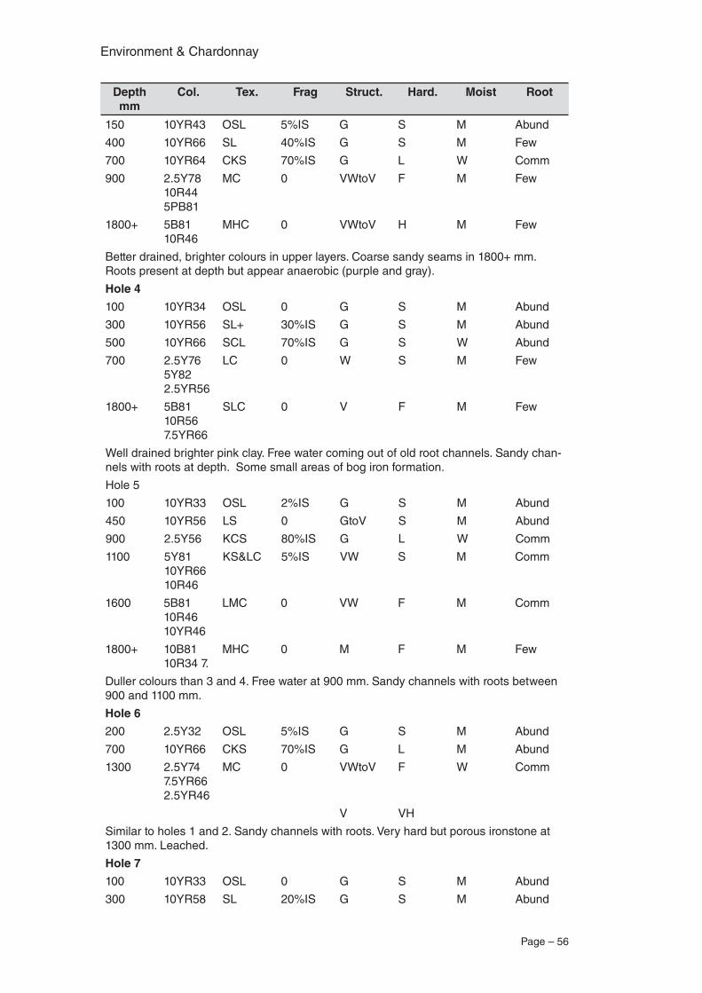
Environment & Chardonnay
Page – 56
Depth mm
Col. Tex. Frag Struct. Hard. Moist Root
150 10YR43 OSL 5%IS G S M Abund
400 10YR66 SL 40%IS G S M Few
700 10YR64 CKS 70%IS G L W Comm
900 2.5Y78 10R44 5PB81
MC 0 VWtoV F M Few
1800+ 5B81 10R46
MHC 0 VWtoV H M Few
Better drained, brighter colours in upper layers. Coarse sandy seams in 1800+ mm. Roots present at depth but appear anaerobic (purple and gray).
Hole 4
100 10YR34 OSL 0 G S M Abund
300 10YR56 SL+ 30%IS G S M Abund
500 10YR66 SCL 70%IS G S W Abund
700 2.5Y76 5Y82 2.5YR56
LC 0 W S M Few
1800+ 5B81 10R56 7.5YR66
SLC 0 V F M Few
Well drained brighter pink clay. Free water coming out of old root channels. Sandy chan-nels with roots at depth. Some small areas of bog iron formation.
Hole 5
100 10YR33 OSL 2%IS G S M Abund
450 10YR56 LS 0 GtoV S M Abund
900 2.5Y56 KCS 80%IS G L W Comm
1100 5Y81 10YR66 10R46
KS&LC 5%IS VW S M Comm
1600 5B81 10R46 10YR46
LMC 0 VW F M Comm
1800+ 10B81 10R34 7.
MHC 0 M F M Few
Duller colours than 3 and 4. Free water at 900 mm. Sandy channels with roots between 900 and 1100 mm.
Hole 6
200 2.5Y32 OSL 5%IS G S M Abund
700 10YR66 CKS 70%IS G L M Abund
1300 2.5Y74 7.5YR66 2.5YR46
MC 0 VWtoV F W Comm
V VH
Similar to holes 1 and 2. Sandy channels with roots. Very hard but porous ironstone at 1300 mm. Leached.
Hole 7
100 10YR33 OSL 0 G S M Abund
300 10YR58 SL 20%IS G S M Abund
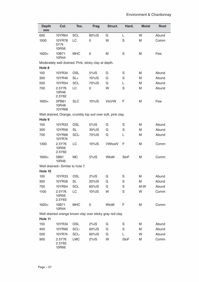
Page – 57
Environment & Chardonnay
Depth mm
Col. Tex. Frag Struct. Hard. Moist Root
600 10YR64 SCL 80%IS G L W Abund
1000 10YR78 5Y74 10R56
LC 0 W S M Comm
1600+ 10B71 10R44
MHC 0 M S M Few
Moderately well drained. Pink, sticky clay at depth.
Hole 8
100 10YR34 OSL 5%IS G S M Abund
300 10YR46 SL+ 10%IS G S M Abund
500 10YR54 SCL 70%IS G L M Abund
700 2.5Y76 10R46 2.5Y82
LC 0 W S M Abund
1600+ 5PB81 10R48 10YR68
SLC 10%IS VtoVW F M Few
Well drained. Orange, crumbly top soil over soft, pink clay.
Hole 9
150 10YR33 OSL 5%IS G S M Abund
300 10YR56 SL 30%IS G S M Abund
700 10YR66 10YR74
SCL- 70%IS G L M Abund
1300 2.5Y76 10R56 2.5Y82
LC 10%IS VWtoslV F M Comm
1600+ 5B81 10R46
MC 5%IS WtoM StoF M Comm
Well drained> Similar to hole 7.
Hole 10
100 10YR33 OSL 2%IS G S M Abund
300 10YR56 SL 20%IS G S M Abund
700 10YR64 SCL 60%IS G S M-W Abund
1100 2.5Y76 10R56 2.5Y83
LC 10%IS W S W Comm
1600+ 10B71 10R44
MHC 0 WtoM F M Comm
Well drained orange brown clay over sticky gray red clay.
Hole 11
150 10YR34 OSL 2%IS G S M Abund
400 10YR66 SCL- 60%IS G S M Abund
500 10YR74 SCL- 60%IS G L W Abund
900 2.5Y76 2.5Y82 10R66
LMC 2%IS W StoF M Comm
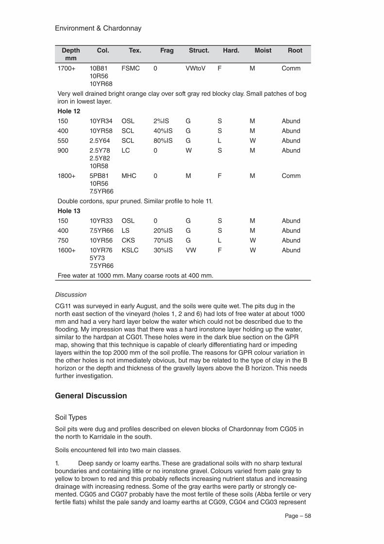
Environment & Chardonnay
Page – 58
Depth mm
Col. Tex. Frag Struct. Hard. Moist Root
1700+ 10B81 10R56 10YR68
FSMC 0 VWtoV F M Comm
Very well drained bright orange clay over soft gray red blocky clay. Small patches of bog iron in lowest layer.
Hole 12
150 10YR34 OSL 2%IS G S M Abund
400 10YR58 SCL 40%IS G S M Abund
550 2.5Y64 SCL 80%IS G L W Abund
900 2.5Y78 2.5Y82 10R58
LC 0 W S M Abund
1800+ 5PB81 10R56 7.5YR66
MHC 0 M F M Comm
Double cordons, spur pruned. Similar profile to hole 11.
Hole 13
150 10YR33 OSL 0 G S M Abund
400 7.5YR66 LS 20%IS G S M Abund
750 10YR56 CKS 70%IS G L W Abund
1600+ 10YR76 5Y73 7.5YR66
KSLC 30%IS VW F W Abund
Free water at 1000 mm. Many coarse roots at 400 mm.
Discussion
CG11 was surveyed in early August, and the soils were quite wet. The pits dug in the north east section of the vineyard (holes 1, 2 and 6) had lots of free water at about 1000 mm and had a very hard layer below the water which could not be described due to the flooding. My impression was that there was a hard ironstone layer holding up the water, similar to the hardpan at CG01. These holes were in the dark blue section on the GPR map, showing that this technique is capable of clearly differentiating hard or impeding layers within the top 2000 mm of the soil profile. The reasons for GPR colour variation in the other holes is not immediately obvious, but may be related to the type of clay in the B horizon or the depth and thickness of the gravelly layers above the B horizon. This needs further investigation.
General Discussion
Soil Types
Soil pits were dug and profiles described on eleven blocks of Chardonnay from CG05 in the north to Karridale in the south.
Soils encountered fell into two main classes.
1. Deep sandy or loamy earths. These are gradational soils with no sharp textural boundaries and containing little or no ironstone gravel. Colours varied from pale gray to yellow to brown to red and this probably reflects increasing nutrient status and increasing drainage with increasing redness. Some of the gray earths were partly or strongly ce-mented. CG05 and CG07 probably have the most fertile of these soils (Abba fertile or very fertile flats) whilst the pale sandy and loamy earths at CG09, CG04 and CG03 represent
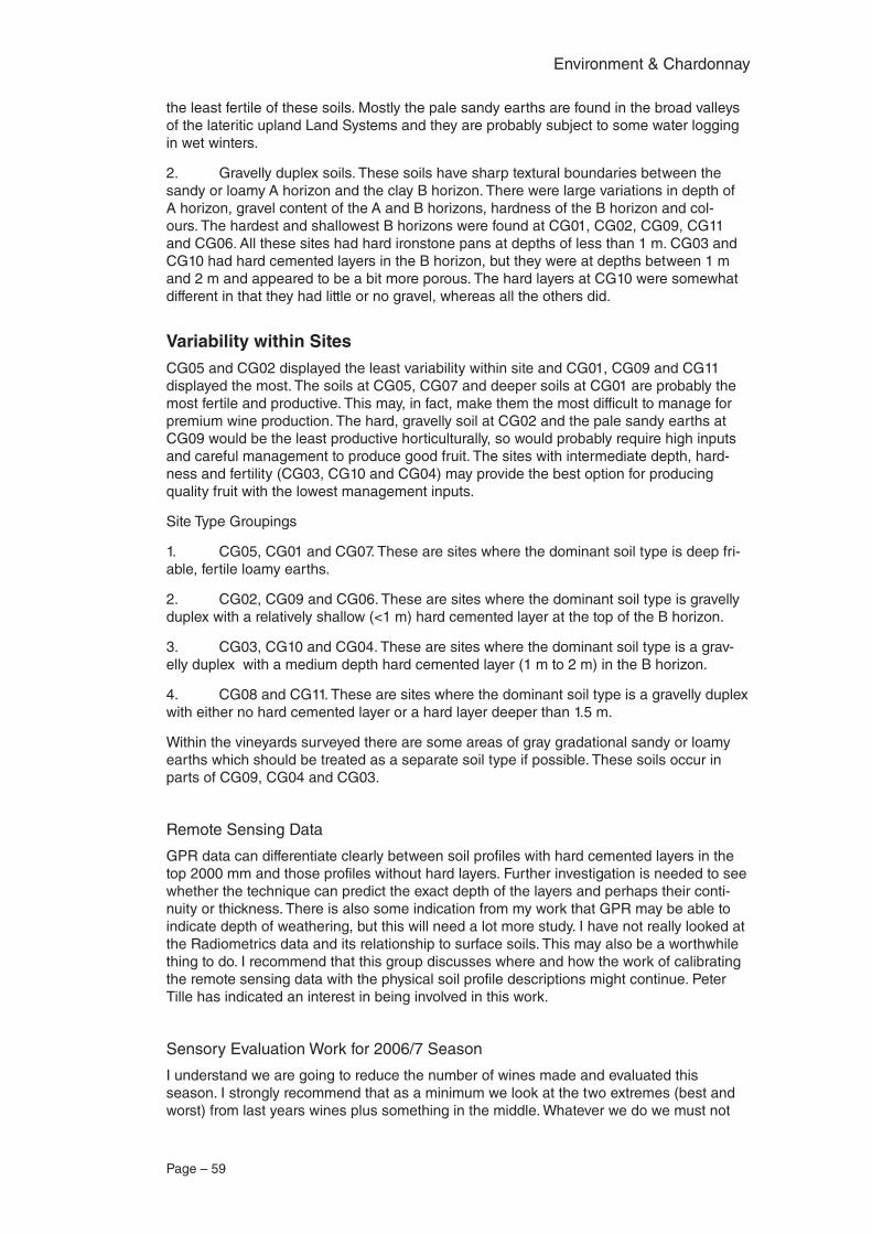
Page – 59
Environment & Chardonnay
the least fertile of these soils. Mostly the pale sandy earths are found in the broad valleys of the lateritic upland Land Systems and they are probably subject to some water logging in wet winters.
2. Gravelly duplex soils. These soils have sharp textural boundaries between the sandy or loamy A horizon and the clay B horizon. There were large variations in depth of A horizon, gravel content of the A and B horizons, hardness of the B horizon and col-ours. The hardest and shallowest B horizons were found at CG01, CG02, CG09, CG11 and CG06. All these sites had hard ironstone pans at depths of less than 1 m. CG03 and CG10 had hard cemented layers in the B horizon, but they were at depths between 1 m and 2 m and appeared to be a bit more porous. The hard layers at CG10 were somewhat different in that they had little or no gravel, whereas all the others did.
Variability within Sites CG05 and CG02 displayed the least variability within site and CG01, CG09 and CG11 displayed the most. The soils at CG05, CG07 and deeper soils at CG01 are probably the most fertile and productive. This may, in fact, make them the most difficult to manage for premium wine production. The hard, gravelly soil at CG02 and the pale sandy earths at CG09 would be the least productive horticulturally, so would probably require high inputs and careful management to produce good fruit. The sites with intermediate depth, hard-ness and fertility (CG03, CG10 and CG04) may provide the best option for producing quality fruit with the lowest management inputs.
Site Type Groupings
1. CG05, CG01 and CG07. These are sites where the dominant soil type is deep fri-able, fertile loamy earths.
2. CG02, CG09 and CG06. These are sites where the dominant soil type is gravelly duplex with a relatively shallow (<1 m) hard cemented layer at the top of the B horizon.
3. CG03, CG10 and CG04. These are sites where the dominant soil type is a grav-elly duplex with a medium depth hard cemented layer (1 m to 2 m) in the B horizon.
4. CG08 and CG11. These are sites where the dominant soil type is a gravelly duplex with either no hard cemented layer or a hard layer deeper than 1.5 m.
Within the vineyards surveyed there are some areas of gray gradational sandy or loamy earths which should be treated as a separate soil type if possible. These soils occur in parts of CG09, CG04 and CG03.
Remote Sensing Data
GPR data can differentiate clearly between soil profiles with hard cemented layers in the top 2000 mm and those profiles without hard layers. Further investigation is needed to see whether the technique can predict the exact depth of the layers and perhaps their conti-nuity or thickness. There is also some indication from my work that GPR may be able to indicate depth of weathering, but this will need a lot more study. I have not really looked at the Radiometrics data and its relationship to surface soils. This may also be a worthwhile thing to do. I recommend that this group discusses where and how the work of calibrating the remote sensing data with the physical soil profile descriptions might continue. Peter Tille has indicated an interest in being involved in this work.
Sensory Evaluation Work for 2006/7 Season
I understand we are going to reduce the number of wines made and evaluated this season. I strongly recommend that as a minimum we look at the two extremes (best and worst) from last years wines plus something in the middle. Whatever we do we must not
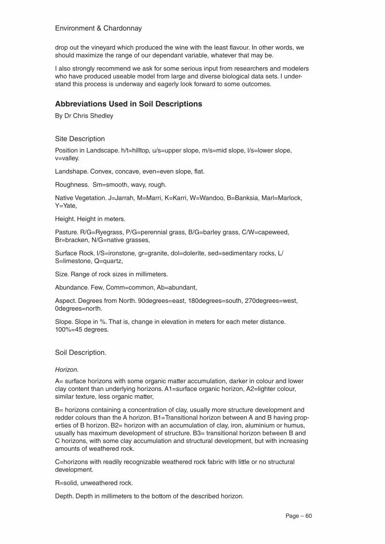
Environment & Chardonnay
Page – 60
drop out the vineyard which produced the wine with the least flavour. In other words, we should maximize the range of our dependant variable, whatever that may be.
I also strongly recommend we ask for some serious input from researchers and modelers who have produced useable model from large and diverse biological data sets. I under-stand this process is underway and eagerly look forward to some outcomes.
Abbreviations Used in Soil DescriptionsBy Dr Chris Shedley
Site Description
Position in Landscape. h/t=hilltop, u/s=upper slope, m/s=mid slope, l/s=lower slope, v=valley.
Landshape. Convex, concave, even=even slope, flat.
Roughness. Sm=smooth, wavy, rough.
Native Vegetation. J=Jarrah, M=Marri, K=Karri, W=Wandoo, B=Banksia, Marl=Marlock, Y=Yate,
Height. Height in meters.
Pasture. R/G=Ryegrass, P/G=perennial grass, B/G=barley grass, C/W=capeweed, Br=bracken, N/G=native grasses,
Surface Rock. I/S=ironstone, gr=granite, dol=dolerite, sed=sedimentary rocks, L/S=limestone, Q=quartz,
Size. Range of rock sizes in millimeters.
Abundance. Few, Comm=common, Ab=abundant,
Aspect. Degrees from North. 90degrees=east, 180degrees=south, 270degrees=west, 0degrees=north.
Slope. Slope in %. That is, change in elevation in meters for each meter distance. 100%=45 degrees.
Soil Description.
Horizon.
A= surface horizons with some organic matter accumulation, darker in colour and lower clay content than underlying horizons. A1=surface organic horizon, A2=lighter colour, similar texture, less organic matter,
B= horizons containing a concentration of clay, usually more structure development and redder colours than the A horizon. B1=Transitional horizon between A and B having prop-erties of B horizon. B2= horizon with an accumulation of clay, iron, aluminium or humus, usually has maximum development of structure. B3= transitional horizon between B and C horizons, with some clay accumulation and structural development, but with increasing amounts of weathered rock.
C=horizons with readily recognizable weathered rock fabric with little or no structural development.
R=solid, unweathered rock.
Depth. Depth in millimeters to the bottom of the described horizon.
Page – 61
Environment & Chardonnay
Colour 1. Dominant colour or matrix colour of horizon. Expressed as Munsell colours as described in the “Munsell Soil Colour Chart 1994.”
Example 5Y32 is Hue= 5Y, Value= 3, Chroma= 2. This colour is described as Olive gray.
Colour 2. Colour of main mottle, with proportion of mottle expressed in %. Second mottle and % often listed in this column.
Gravel%. Percentage of horizon by weight that is gravel or rock fragments. Type of frag-ment in brackets. IS=ironstone, R=parent rock fragments, Q=quartz.
Texture. In order of increasing clay content. S=sand, LS=loamy sand, CS=clayey sand, SL=sandy loam, L=loam, ZL=silty loam, SCL=sandy clay loam, CL=clay loam, CLS=clay loam sandy, ZCL=silty clay loam, LC=light clay, LMC=light medium clay, MC=medium clay, MHC=medium heavy clay, HC=heavy clay. Modifiers K=coarse, F=fine when describ-ing sand. -=lighter, +=heavier when describing clay content.
Structure. G=single grain, V=massive, W=weak, M=moderate, S=strong.
Hardness. L=loose, S=soft, F=firm, H=hard, VH=very hard, #=impenetrable with backhoe.
Moisture. D=dry, SlM=slightly moist, M=-moist, W=wet, FW=free water.
Roots. N=none, F=few, C=common, Ab=abundant.
Definitions
For definitions of all terms used in soil descriptions see the book “Australian Soil and Land Survey-Field Handbook.” Second Edition.
By R.C.McDonald, R.F.Isbell, J.G.Speight, J.Walker and M.S.Hopkins.
Published by Inkata Press. 1990.
For descriptions of soil colour see “Munsell Soil Colour Charts” 1994, Revised Edition. Produced by Kollmorgen Instruments Corporation.

Environment & Chardonnay
Page – 62
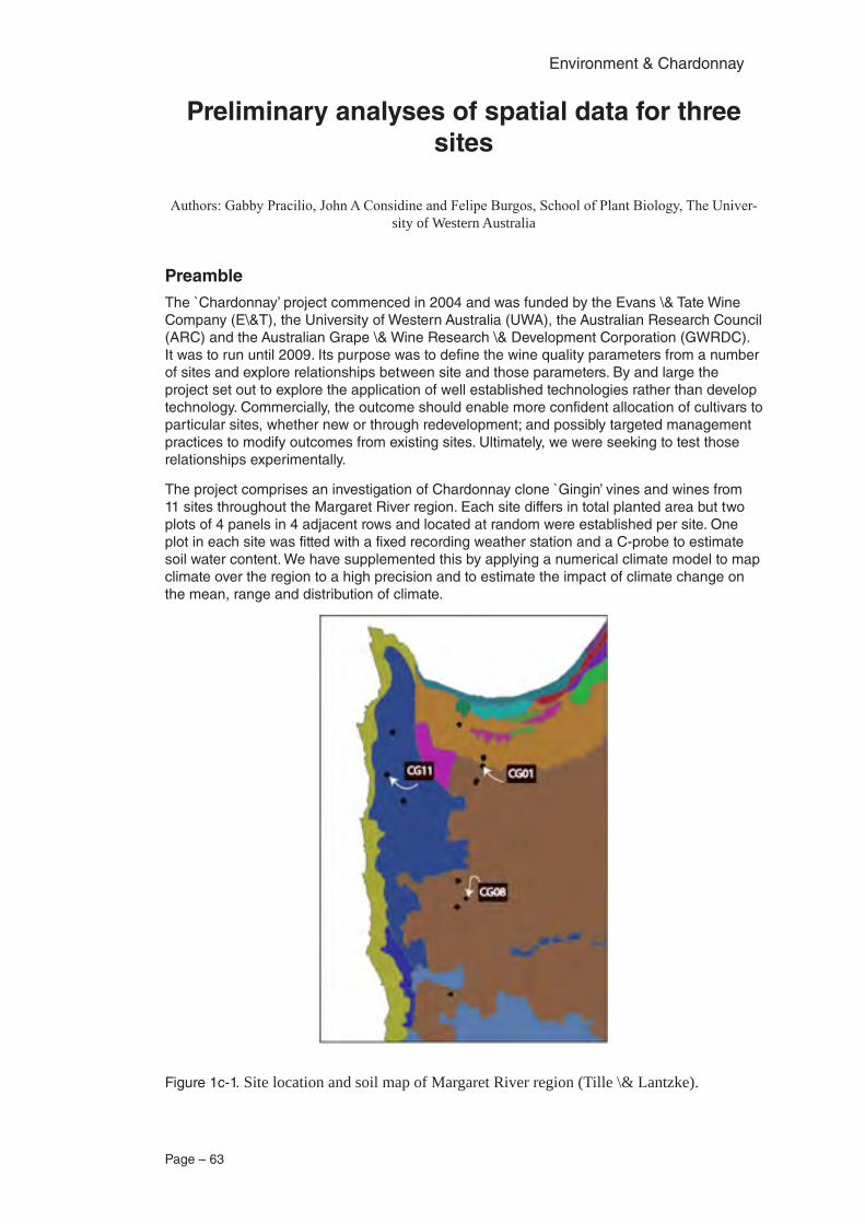
Page – 63
Environment & Chardonnay
Preliminary analyses of spatial data for three sites
Authors: Gabby Pracilio, John A Considine and Felipe Burgos, School of Plant Biology, The Univer-sity of Western Australia
PreambleThe `Chardonnay’ project commenced in 2004 and was funded by the Evans \& Tate Wine Company (E\&T), the University of Western Australia (UWA), the Australian Research Council (ARC) and the Australian Grape \& Wine Research \& Development Corporation (GWRDC). It was to run until 2009. Its purpose was to define the wine quality parameters from a number of sites and explore relationships between site and those parameters. By and large the project set out to explore the application of well established technologies rather than develop technology. Commercially, the outcome should enable more confident allocation of cultivars to particular sites, whether new or through redevelopment; and possibly targeted management practices to modify outcomes from existing sites. Ultimately, we were seeking to test those relationships experimentally.
The project comprises an investigation of Chardonnay clone `Gingin’ vines and wines from 11 sites throughout the Margaret River region. Each site differs in total planted area but two plots of 4 panels in 4 adjacent rows and located at random were established per site. One plot in each site was fitted with a fixed recording weather station and a C-probe to estimate soil water content. We have supplemented this by applying a numerical climate model to map climate over the region to a high precision and to estimate the impact of climate change on the mean, range and distribution of climate.
Figure 1c-1. Site location and soil map of Margaret River region (Tille \& Lantzke).
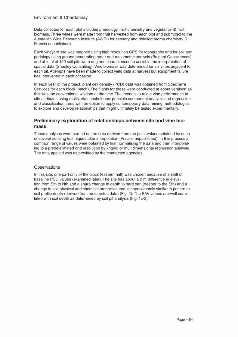
Environment & Chardonnay
Page – 64
Data collected for each plot included phenology, fruit chemistry and vegetative \& fruit biomass. Three wines were made from fruit harvested from each plot and submitted to the Australian Wine Research Institute (AWRI) for sensory and detailed aroma chemistry (L. Francis unpublished).
Each vineyard site was mapped using high resolution GPS for topography and for soil and pedology using ground penetrating radar and radiometric analysis (Baigent Geosciences) and at total of 120 soil pits were dug and characterised to assist in the interpretation of spatial data (Shedley Consulting). Vine biomass was determined for six vines adjacent to each pit. Attempts have been made to collect yield data at harvest but equipment failure has intervened in each occasion.
In each year of the project, plant cell density (PCD) data was obtained from SpecTerra Services for each block (patch). The flights for these were conducted at about veraison as this was the conventional wisdom at the time. The intent is to relate vine performance to site attributes using multivariate techniques: principle component analysis and regression and classification trees with an option to apply contemporary data mining methodologies to explore and develop relationships that might ultimately be tested experimentally.
Preliminary exploration of relationships between site and vine bio-mass.These analyses were carried out on data derived from the point values obtained by each of several sensing techniques after interpolation (Pracilio unpublished). In this process a common range of values were obtained by first normalising the data and then interpolat-ing to a predetermined grid resolution by kriging or multidimensional regression analysis. The data applied was as provided by the contracted agencies.
Observations
In this site, one part only of the block (eastern half) was chosen because of a shift of baseline PCD values (examined later). The site has about a 2 m difference in eleva-tion from Sth to Nth and a sharp change in depth to hard pan (deeper to the Sth) and a change in soil physical and chemical properties that is approximately similar in pattern to soil profile depth (derived from radiometric data) (Fig. 2). The SAV values are well corre-lated with soil depth as determined by soil pit analysis (Fig. 1c-3).
Page – 65
Environment & Chardonnay
130 m
H igh
Low
H igh : 59 .6m
Low : 57 .4m
Shallow
Deep
A
B
C
Figure 1c-2. Elevation, digital elevation value, DEM (A), structural activity value (SAV, B) and total radiometric count (C) for the eastern half of site CG01.
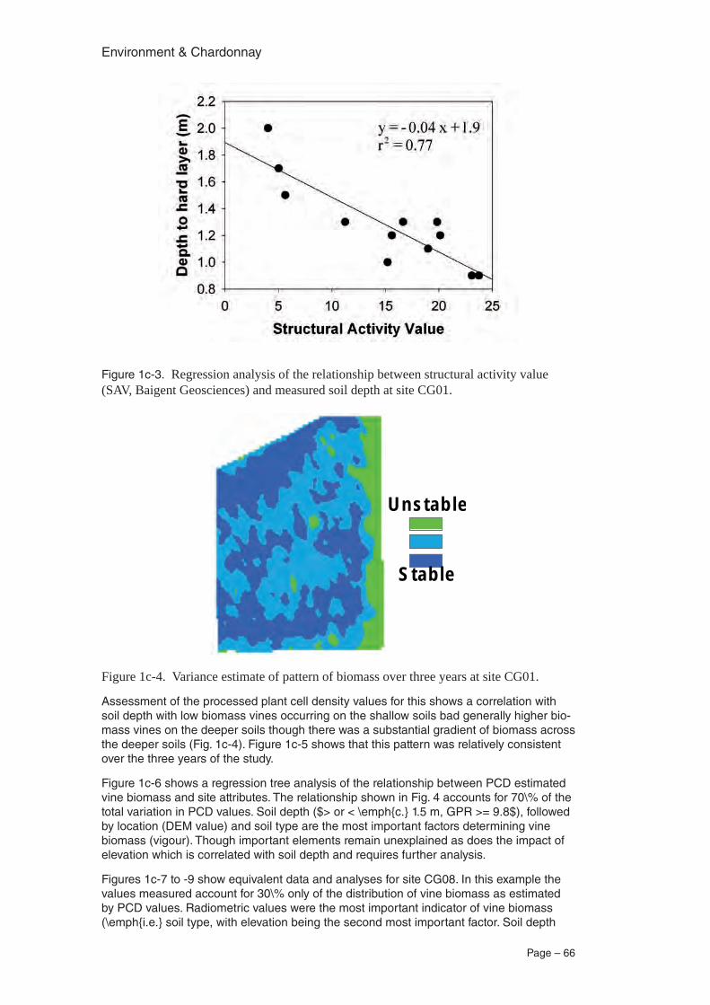
Environment & Chardonnay
Page – 66
Figure 1c-3. Regression analysis of the relationship between structural activity value (SAV, Baigent Geosciences) and measured soil depth at site CG01.
Unstab le
S tab le
Figure 1c-4. Variance estimate of pattern of biomass over three years at site CG01.
Assessment of the processed plant cell density values for this shows a correlation with soil depth with low biomass vines occurring on the shallow soils bad generally higher bio-mass vines on the deeper soils though there was a substantial gradient of biomass across the deeper soils (Fig. 1c-4). Figure 1c-5 shows that this pattern was relatively consistent over the three years of the study.
Figure 1c-6 shows a regression tree analysis of the relationship between PCD estimated vine biomass and site attributes. The relationship shown in Fig. 4 accounts for 70\% of the total variation in PCD values. Soil depth ($> or < \emph{c.} 1.5 m, GPR >= 9.8$), followed by location (DEM value) and soil type are the most important factors determining vine biomass (vigour). Though important elements remain unexplained as does the impact of elevation which is correlated with soil depth and requires further analysis.
Figures 1c-7 to -9 show equivalent data and analyses for site CG08. In this example the values measured account for 30\% only of the distribution of vine biomass as estimated by PCD values. Radiometric values were the most important indicator of vine biomass (\emph{i.e.} soil type, with elevation being the second most important factor. Soil depth
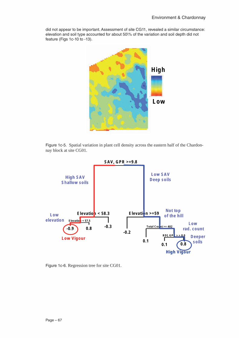
Page – 67
Environment & Chardonnay
did not appear to be important. Assessment of site CG11, revealed a similar circumstance: elevation and soil type accounted for about 50\% of the variation and soil depth did not feature (Figs 1c-10 to -13).
H igh
Low
Figure 1c-5. Spatial variation in plant cell density across the eastern half of the Chardon-nay block at site CG01.
E levation >=59E levation < 58.3
S AV , G P R >=9.8
E levation < 57 .5
Tota l C ou nt >= 402
R D I, G P R > = 8 .0
0 .80 .10.1
-0 .2-0 .30.8-0 .9
E levation >=59E levation < 58.3
S AV , G P R >=9.8
E levation < 57 .5
Tota l C ou nt >= 402
R D I, G P R > = 8 .0
0 .80 .10.1
-0 .2-0 .30.8-0 .9
Low V igour
H igh S AVS h allow so ils
Low elevation
Low V igour
H igh S AVS h allow so ils
Low elevation
H igh V igour
Low S AVD eep so ils
N ot top o f the h ill
Low rad . count
D eeper so ils
H igh V igour
Low S AVD eep so ils
N ot top o f the h ill
Low rad . count
D eeper so ils
Figure 1c-6. Regression tree for site CG01.
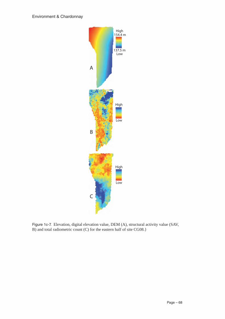
Environment & Chardonnay
Page – 68
High
Low
High
Low
High
Low
154.4 m
137.5 m
A
B
C
Figure 1c-7. Elevation, digital elevation value, DEM (A), structural activity value (SAV, B) and total radiometric count (C) for the eastern half of site CG08.}
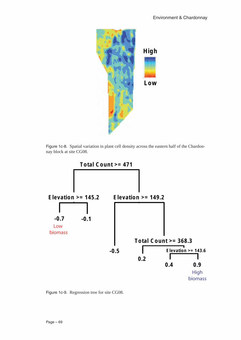
Page – 69
Environment & Chardonnay
H igh
Low
Figure 1c-8. Spatial variation in plant cell density across the eastern half of the Chardon-nay block at site CG08.
Total C ount >= 471
E levation >= 149.2E levation >= 145.2
Tota l C ount >= 368.3E levation >= 143.6
-0 .7 -0 .1
-0 .50.2
0.4 0.9
To ta l C ount >= 471
E levation >= 149.2
Tota l C ount >= 368.3E levation >= 143.6
-0 .7 -0 .1
-0 .50.2
0.4 0.9
Low biomass
Highbiomass
Figure 1c-9. Regression tree for site CG08.
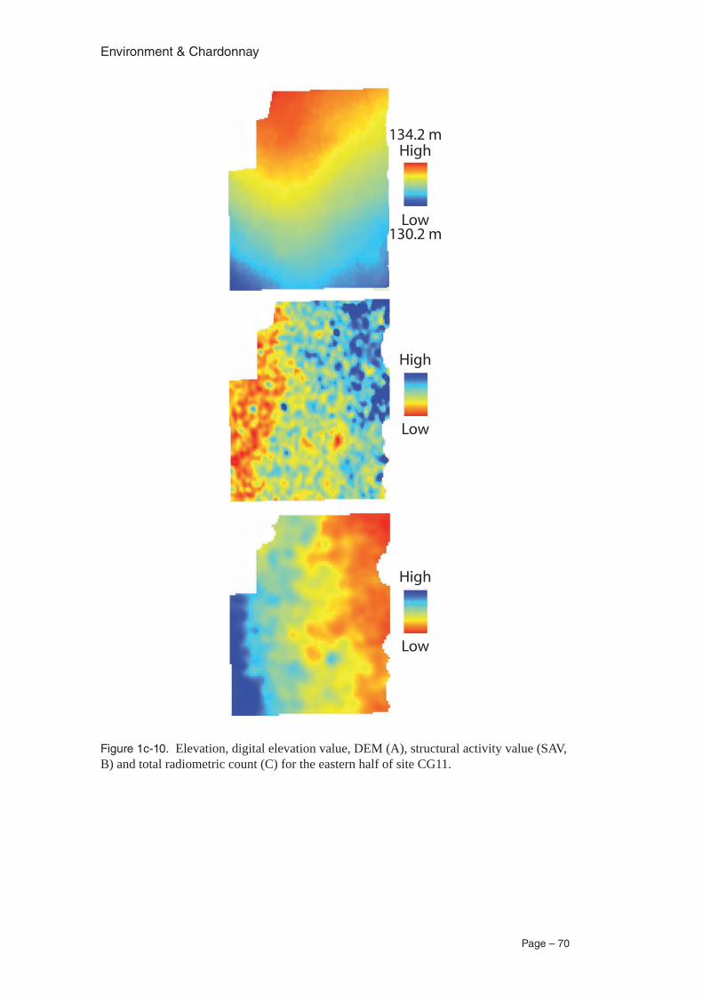
Environment & Chardonnay
Page – 70
High
Low
High
Low
High
Low
134.2 m
130.2 m
Figure 1c-10. Elevation, digital elevation value, DEM (A), structural activity value (SAV, B) and total radiometric count (C) for the eastern half of site CG11.
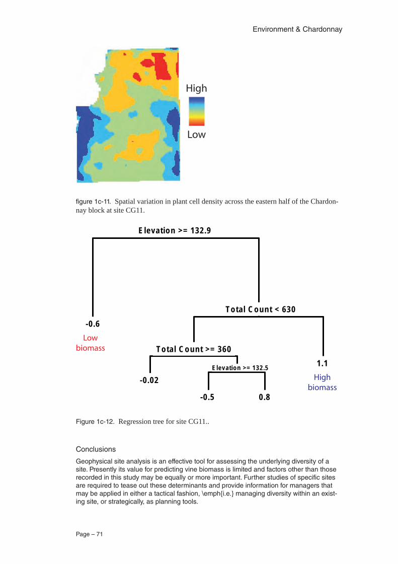
Page – 71
Environment & Chardonnay
High
Low
figure 1c-11. Spatial variation in plant cell density across the eastern half of the Chardon-nay block at site CG11.
Total C ount < 630
E levation >= 132.9
E levation >= 132.5
To ta l C ount >= 360
-0 .6
-0 .02
-0 .5 0.8
1.1
To ta l C ount < 630
E levation >= 132.9
E levation >= 132.5
To ta l C ount >= 360
-0 .6
-0 .02
-0 .5 0.8
1.1
Lowbiomass
Highbiomass
Figure 1c-12. Regression tree for site CG11..
Conclusions
Geophysical site analysis is an effective tool for assessing the underlying diversity of a site. Presently its value for predicting vine biomass is limited and factors other than those recorded in this study may be equally or more important. Further studies of specific sites are required to tease out these determinants and provide information for managers that may be applied in either a tactical fashion, \emph{i.e.} managing diversity within an exist-ing site, or strategically, as planning tools.
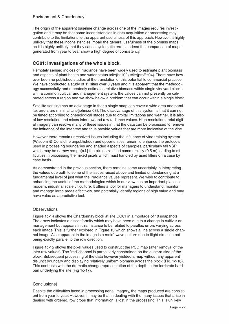
Environment & Chardonnay
Page – 72
The origin of the apparent baseline change across one of the images requires investi-gation and it may be that some inconsistencies in data acquisition or processing may contribute to the limitations to the apparent usefulness of this approach. However, it highly unlikely that these inconsistencies impair the general usefulness of the biomass maps, as it is highly unlikely that they cause systematic errors. Indeed the comparison of maps generated from year to year show a high degree of consistency.
CG01: Investigations of the whole block.Remotely sensed indices of irradiance have been widely used to estimate plant biomass and aspects of plant health and water status \cite{hall02} \cite{proffitt04}. There have how-ever been no published studies of the translation of this potential to commercial practice. We have conducted a study of 11 sites over 3 years and it is apparent that the methodol-ogy successfully and repeatedly estimates relative biomass within single vineyard blocks with a common cultivar and management system, the values can not presently be cali-brated across a region and we show below a problem that can occur within a single block.
Satellite sensing has an advantage in that a single snap can cover a wide area and paral-lax errors are minimal \cite{johnson03}. The disadvantage of this system is that it can not be timed according to phenological stages due to orbital limitations and weather. It is also of low resolution and mixes inter-row and row radiance values. High resolution aerial digit-al imagery can resolve many of these issues in that the data can be processed to remove the influence of the inter-row and thus provide values that are more indicative of the vine.
However there remain unresolved issues including the influence of vine training system (Wisdom \& Considine unpublished) and opportunities remain to enhance the protocols used in processing boundaries and shaded aspects of canopies, particularly tall VSP which may be narrow \emph{c.f.} the pixel size used commercially (0.5 m) leading to dif-ficulties in processing the mixed pixels which must handled by used filters on a case by case basis.
As demonstrated in the previous section, there remains some uncertainly in interpreting the values due both to some of the issues raised above and limited understanding at a fundamental level of just what the irradiance values represent. We wish to contribute to enhancing the useful of the methodologies which in our view has an important place in modern, industrial scale viticulture. It offers a tool for managers to understand, monitor and manage large areas effectively, and potentially identify regions of high value and may have value as a predictive tool.
Observations
Figure 1c-14 shows the Chardonnay block at site CG01 in a montage of 10 snapshots. The arrow indicates a disconformity which may have been due to a change in cultivar or management but appears in this instance to be related to parallax errors varying across each image. This is further explored in Figure 13 which shows a line across a single chan-nel image. Also apparent in the image is a moiré wave pattern due to flight direction not being exactly parallel to the row direction.
Figure 1c-15 shows the pixel values used to construct the PCD map (after removal of the inter-row values). The `red’ channel is particularly constrained on the eastern side of the block. Subsequent processing of the data however yielded a map without any apparent disjunct boundary and displaying relatively uniform biomass across the block (Fig. 1c-16). This contrasts with the dramatic change representation of the depth to the ferricrete hard-pan underlying the site (Fig 1c-17).
Conclusions}
Despite the difficulties faced in processing aerial imagery, the maps produced are consist-ent from year to year. However, it may be that in dealing with the many issues that arise in dealing with ordered, row crops that information is lost in the processing. This is unlikely
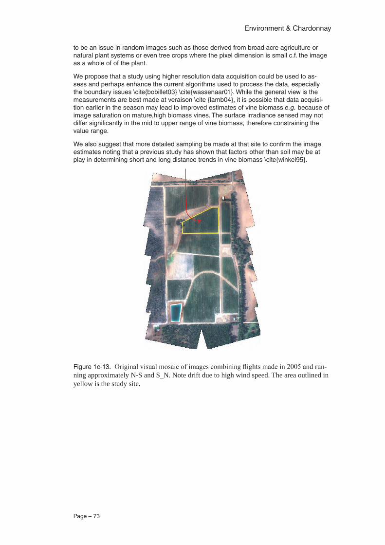
Page – 73
Environment & Chardonnay
to be an issue in random images such as those derived from broad acre agriculture or natural plant systems or even tree crops where the pixel dimension is small c.f. the image as a whole of of the plant.
We propose that a study using higher resolution data acquisition could be used to as-sess and perhaps enhance the current algorithms used to process the data, especially the boundary issues \cite{bobillet03} \cite{wassenaar01}. While the general view is the measurements are best made at veraison \cite {lamb04}, it is possible that data acquisi-tion earlier in the season may lead to improved estimates of vine biomass e.g. because of image saturation on mature,high biomass vines. The surface irradiance sensed may not differ significantly in the mid to upper range of vine biomass, therefore constraining the value range.
We also suggest that more detailed sampling be made at that site to confirm the image estimates noting that a previous study has shown that factors other than soil may be at play in determining short and long distance trends in vine biomass \cite{winkel95}.
Figure 1c-13. Original visual mosaic of images combining flights made in 2005 and run-ning approximately N-S and S_N. Note drift due to high wind speed. The area outlined in yellow is the study site.
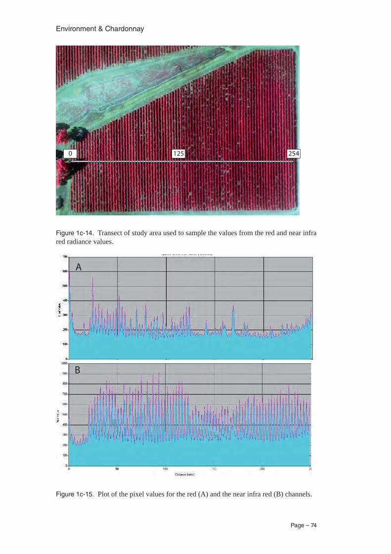
Environment & Chardonnay
Page – 74
0 125 254
Figure 1c-14. Transect of study area used to sample the values from the red and near infra red radiance values.
A
B
Figure 1c-15. Plot of the pixel values for the red (A) and the near infra red (B) channels.
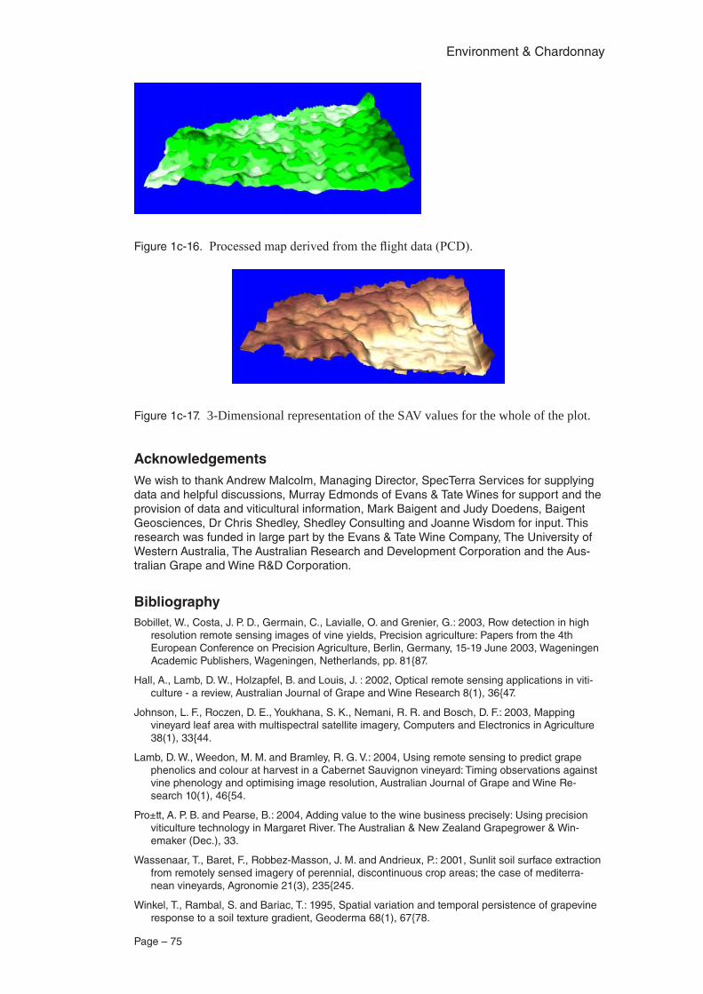
Page – 75
Environment & Chardonnay
Figure 1c-16. Processed map derived from the flight data (PCD).
Figure 1c-17. 3-Dimensional representation of the SAV values for the whole of the plot.
AcknowledgementsWe wish to thank Andrew Malcolm, Managing Director, SpecTerra Services for supplying data and helpful discussions, Murray Edmonds of Evans & Tate Wines for support and the provision of data and viticultural information, Mark Baigent and Judy Doedens, Baigent Geosciences, Dr Chris Shedley, Shedley Consulting and Joanne Wisdom for input. This research was funded in large part by the Evans & Tate Wine Company, The University of Western Australia, The Australian Research and Development Corporation and the Aus-tralian Grape and Wine R&D Corporation.
BibliographyBobillet, W., Costa, J. P. D., Germain, C., Lavialle, O. and Grenier, G.: 2003, Row detection in high
resolution remote sensing images of vine yields, Precision agriculture: Papers from the 4th European Conference on Precision Agriculture, Berlin, Germany, 15-19 June 2003, Wageningen Academic Publishers, Wageningen, Netherlands, pp. 81{87.
Hall, A., Lamb, D. W., Holzapfel, B. and Louis, J. : 2002, Optical remote sensing applications in viti-culture - a review, Australian Journal of Grape and Wine Research 8(1), 36{47.
Johnson, L. F., Roczen, D. E., Youkhana, S. K., Nemani, R. R. and Bosch, D. F.: 2003, Mapping vineyard leaf area with multispectral satellite imagery, Computers and Electronics in Agriculture 38(1), 33{44.
Lamb, D. W., Weedon, M. M. and Bramley, R. G. V.: 2004, Using remote sensing to predict grape phenolics and colour at harvest in a Cabernet Sauvignon vineyard: Timing observations against vine phenology and optimising image resolution, Australian Journal of Grape and Wine Re-search 10(1), 46{54.
Pro±tt, A. P. B. and Pearse, B.: 2004, Adding value to the wine business precisely: Using precision viticulture technology in Margaret River. The Australian & New Zealand Grapegrower & Win-emaker (Dec.), 33.
Wassenaar, T., Baret, F., Robbez-Masson, J. M. and Andrieux, P.: 2001, Sunlit soil surface extraction from remotely sensed imagery of perennial, discontinuous crop areas; the case of mediterra-nean vineyards, Agronomie 21(3), 235{245.
Winkel, T., Rambal, S. and Bariac, T.: 1995, Spatial variation and temporal persistence of grapevine response to a soil texture gradient, Geoderma 68(1), 67{78.

Environment & Chardonnay
Page – 76
Page – 77
Environment & Chardonnay
Ground-truthing Site CG01
Contributing authors J.A Considine, F. Burgos, School of Plant Biology, The University of Western Australia
Abstract
This analysis sets out to examine the relationship between a measured estimate of vine biomass and remotely sensed values (plant cell density, PCD) and further to determine the relationship between sensed soil and elevation parameters and both measured vine biomass and PCD values.
A preliminary assessment of the relationship between site attributes, principally, depth to hard pan as estimated by ground penetrating radar, shows a strong relationship on this site with plant cell density, either raw or processed data. An attempt to ground-truth this observation by measuring two, 2-vine transects (4 m) of the vineyard showed a statisti-cally significant correlation with both parameters, but the greater between-vine variabil-ity in this parameter was not well estimated by the remote sensing techniques. These techniques seem to smooth the observed variation but are non-the-less useful means of representing vine biomass and particular underlying causes of variation in that biomass.
The method chosen for estimating vine biomass was trunk cross section as is widely used in forestry. It’s value lies in its simplicity, cheapness and that it is non-destructive. It was show to be well related to externally sensed biomass (PCD) especially the non-krigged, individual pixel values. However, the krigged, or averaged values were more closely related to site parameters and to more parameters than the trunk measurements, It is also well-related to fresh pruning weight. The relationship between trunk and leaf biomass, especially vertically sensed leaf biomass, is however non-linear.
Future attempts should probably use a wider transect to give a greater opportunity to smooth the vine-vine variations in biomass (e.g. 3 to 4 vines, or 6 to 8 m of canopy)}. Further analysis of the data is required to refine the relationships and especially to exam-ine the soil pit data (see Shedley Section 1B and Pracilio Section 1C) and the data from the plots and the wine data. However it seems clear that PCD values are a fair estimate of vine biomass and are well related to soil parameters that conceivably have an impact on vine biomass, even in irrigated vineyards.
IntroductionPreliminary assessment of spatial data indicated little apparent correlation between PCD val-ues and soil depth and perceptions of spatial variation in yield and maturity. We thus set out to assess methods for examining these relationships on a quantitative basis. While we opted initially for a random plot within each vineyard as the best method of sampling the site, we judged that this this purpose if would be best to use methods widely using in natural systems ecology, line transects. We judged that in the time available the most reasonable measure of vine biomass was trunk diameter, a standard method in forestry.
Materials & Methods
Using a visual assessment of the PCD maps provided by Specterra Services Ltd (January 2007) and the soil depth estimates provided via Ground Penetrating Radar (Baigent Geo-sciences) we drew two East - West Transects (Fig. 1d-1). We located these using a Differen-tial GPS (Delta Systems< 0.1 m resolution).
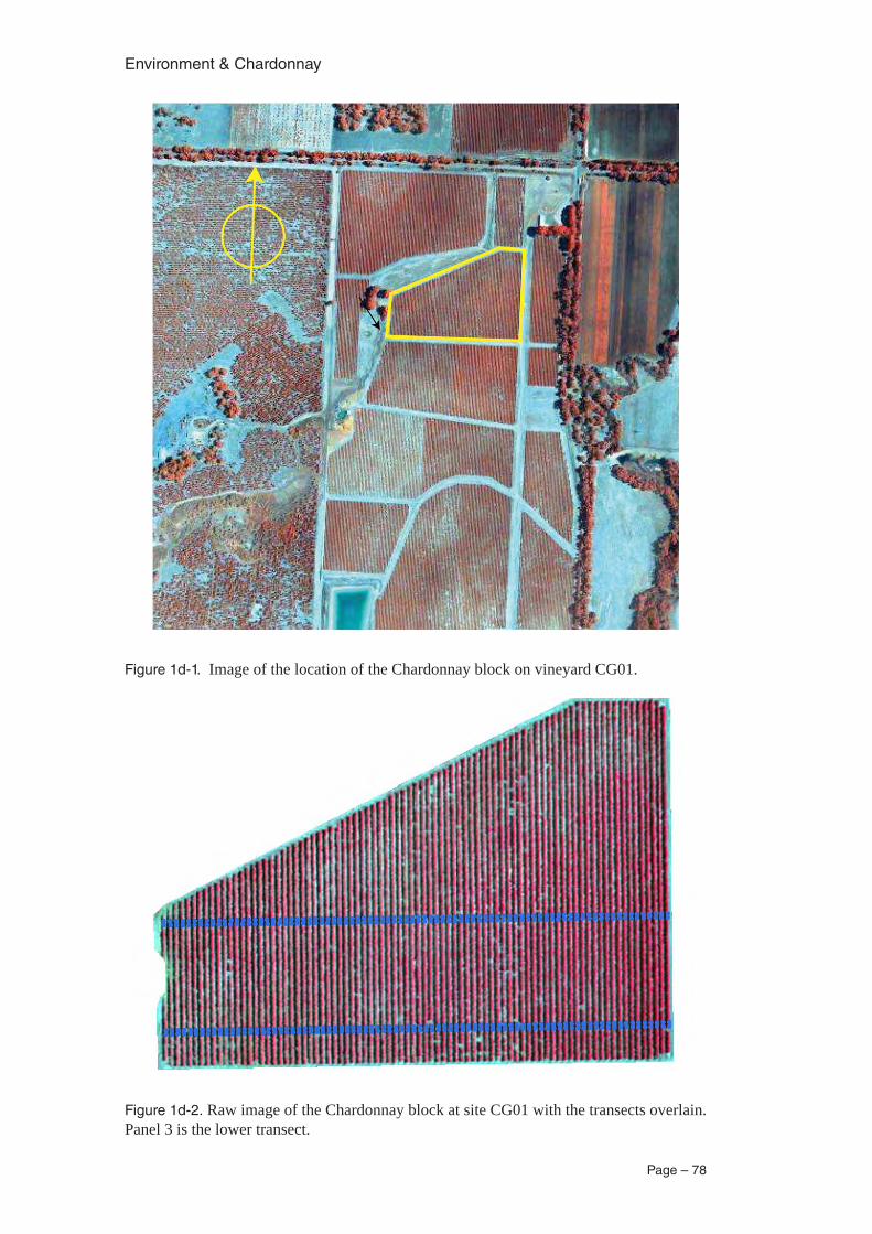
Environment & Chardonnay
Page – 78
Figure 1d-1. Image of the location of the Chardonnay block on vineyard CG01.
Figure 1d-2. Raw image of the Chardonnay block at site CG01 with the transects overlain. Panel 3 is the lower transect.
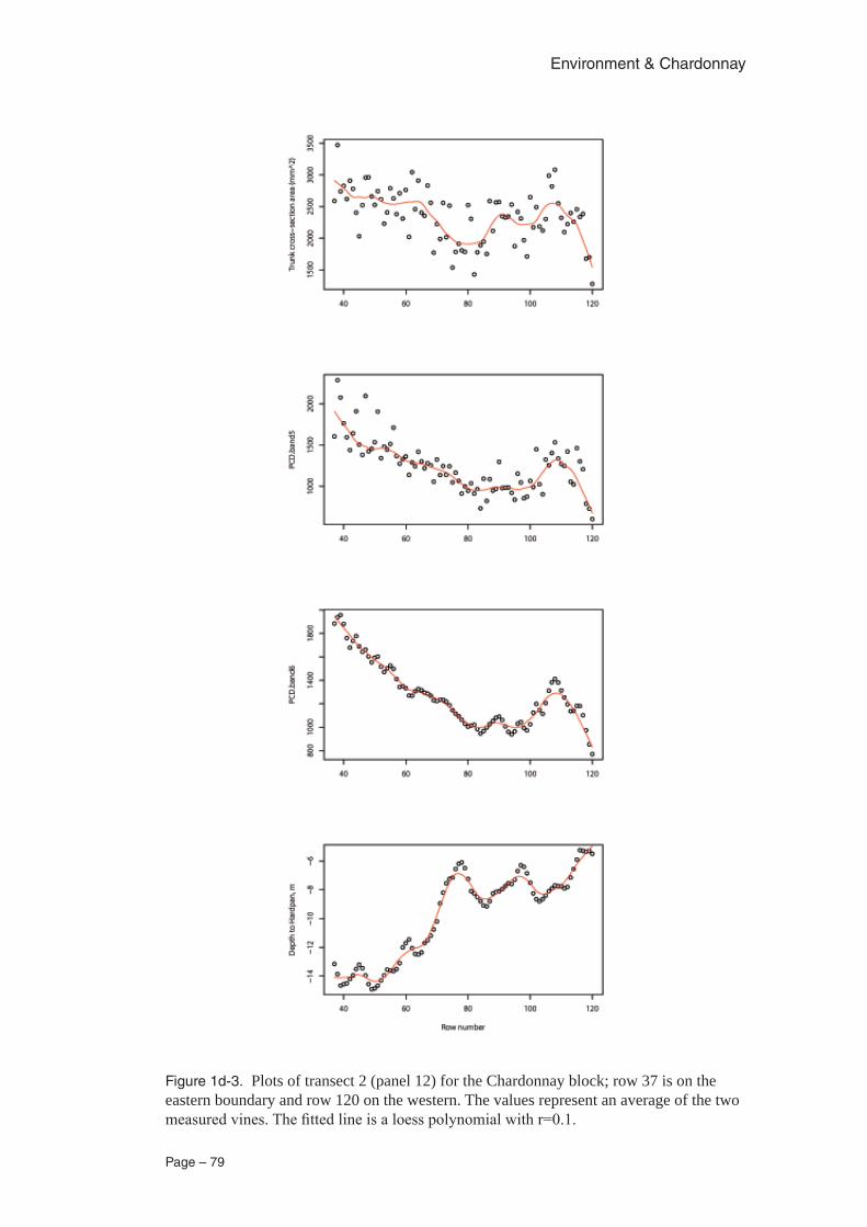
Page – 79
Environment & Chardonnay
Figure 1d-3. Plots of transect 2 (panel 12) for the Chardonnay block; row 37 is on the eastern boundary and row 120 on the western. The values represent an average of the two measured vines. The fitted line is a loess polynomial with r=0.1.
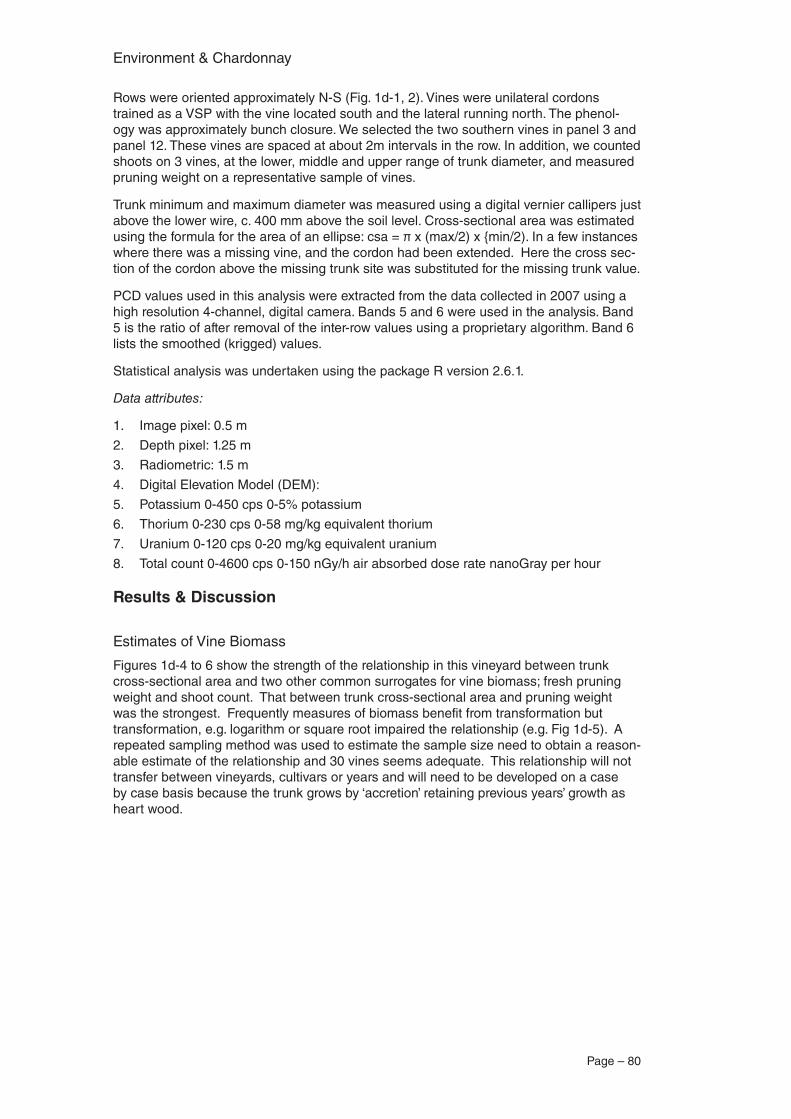
Environment & Chardonnay
Page – 80
Rows were oriented approximately N-S (Fig. 1d-1, 2). Vines were unilateral cordons trained as a VSP with the vine located south and the lateral running north. The phenol-ogy was approximately bunch closure. We selected the two southern vines in panel 3 and panel 12. These vines are spaced at about 2m intervals in the row. In addition, we counted shoots on 3 vines, at the lower, middle and upper range of trunk diameter, and measured pruning weight on a representative sample of vines.
Trunk minimum and maximum diameter was measured using a digital vernier callipers just above the lower wire, c. 400 mm above the soil level. Cross-sectional area was estimated using the formula for the area of an ellipse: csa = π x (max/2) x {min/2). In a few instances where there was a missing vine, and the cordon had been extended. Here the cross sec-tion of the cordon above the missing trunk site was substituted for the missing trunk value.
PCD values used in this analysis were extracted from the data collected in 2007 using a high resolution 4-channel, digital camera. Bands 5 and 6 were used in the analysis. Band 5 is the ratio of after removal of the inter-row values using a proprietary algorithm. Band 6 lists the smoothed (krigged) values.
Statistical analysis was undertaken using the package R version 2.6.1.
Data attributes:
Image pixel: 0.5 m
Depth pixel: 1.25 m
Radiometric: 1.5 m
Digital Elevation Model (DEM):
Potassium 0-450 cps 0-5% potassium
Thorium 0-230 cps 0-58 mg/kg equivalent thorium
Uranium 0-120 cps 0-20 mg/kg equivalent uranium
Total count 0-4600 cps 0-150 nGy/h air absorbed dose rate nanoGray per hour
Results & Discussion
Estimates of Vine Biomass
Figures 1d-4 to 6 show the strength of the relationship in this vineyard between trunk cross-sectional area and two other common surrogates for vine biomass; fresh pruning weight and shoot count. That between trunk cross-sectional area and pruning weight was the strongest. Frequently measures of biomass benefit from transformation but transformation, e.g. logarithm or square root impaired the relationship (e.g. Fig 1d-5). A repeated sampling method was used to estimate the sample size need to obtain a reason-able estimate of the relationship and 30 vines seems adequate. This relationship will not transfer between vineyards, cultivars or years and will need to be developed on a case by case basis because the trunk grows by ‘accretion’ retaining previous years’ growth as heart wood.
1.
2.
3.
4.
5.
6.
7.
8.
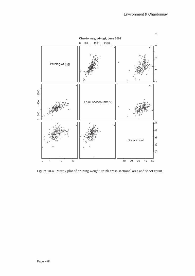
Page – 81
Environment & Chardonnay
Pruning wt (kg)
0 500 1500 2500
01
23
4
050
015
0025
00
Trunk section (mm^2)
0 1 2 34 10 20 30 40 50
1020
3040
50
Shoot count
Chardonnay, vd=cg1, June 2008
Figure 1d-4. Matrix plot of pruning weight, trunk cross-sectional area and shoot count.
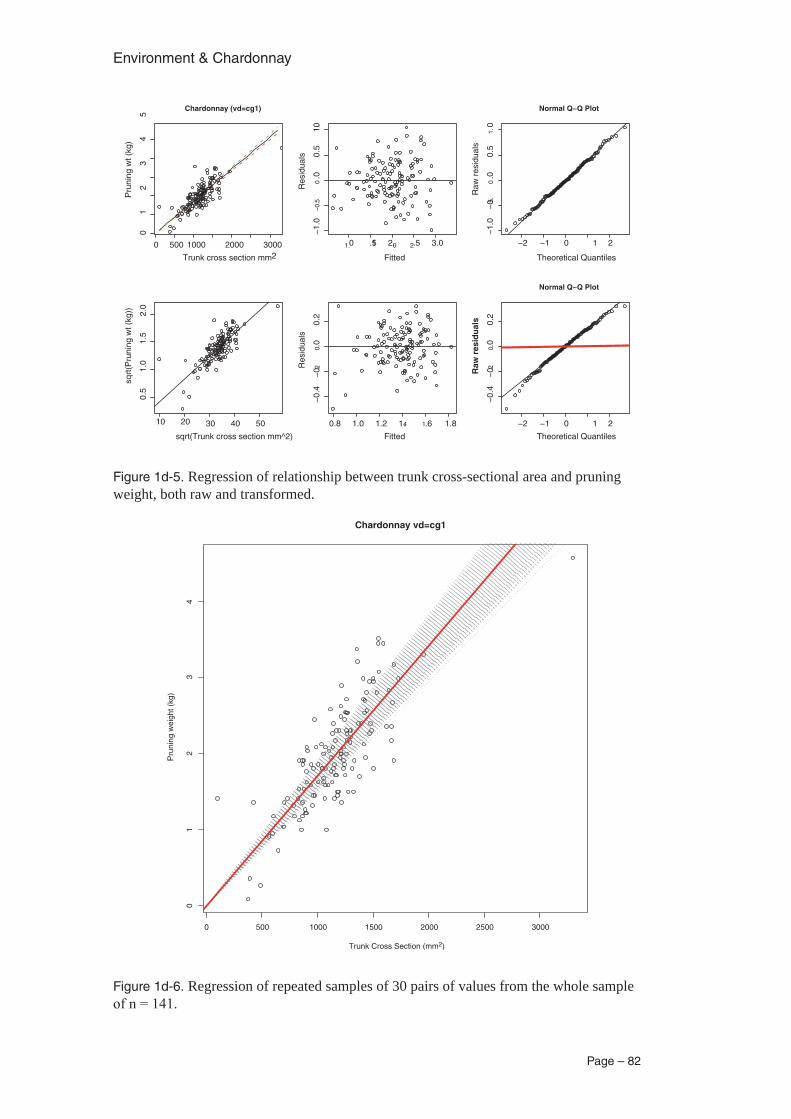
Environment & Chardonnay
Page – 82
0 500 1000 2000 3000
01
23
45
Chardonnay (vd=cg1)
Trunk cross section mm2
Pru
ning
wt (
kg)
1.0 1.5 2.0 2.5 3.0
−1.
0−
0.5
0.0
0.5
1.0
Fitted
Res
idua
ls
−2 −1 0 1 2
−1.
0−
0.50
.00.
51.
0
Normal Q−Q Plot
Theoretical Quantiles
Raw
res
idua
ls
10 20 30 40 50
0.5
1.0
1.5
2.0
sqrt(Trunk cross section mm^2)
sqrt
(Pru
ning
wt (
kg))
0.8 1.0 1.2 1.4 1.6 1.8
−0.
4−
0.20.
00.
2
Fitted
Res
idua
ls
−2 −1 0 1 2
−0.
4−
0.20.
00.
2
Normal Q−Q Plot
Theoretical Quantiles
Raw
res
idu
als
Figure 1d-5. Regression of relationship between trunk cross-sectional area and pruning weight, both raw and transformed.
0 500 1000 1500 2000 2500 3000
01
23
4
Chardonnay vd=cg1
Trunk Cross Section (mm2)
Pru
ning
wei
ght (
kg)
Figure 1d-6. Regression of repeated samples of 30 pairs of values from the whole sample of n = 141.
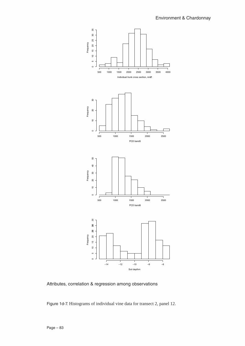
Page – 83
Environment & Chardonnay
Individual trunk cross section, mm2̂
Fre
quen
cy
500 1000 1500 2000 2500 3000 3500 4000
05
1015
2025
3035
PCD band5
Fre
quen
cy
500 1000 1500 2000 2500
010
2030
PCD band6
Fre
quen
cy
500 1000 1500 2000 2500
010
2030
4050
Soil depth m
Fre
quen
cy
−14 −12 −10 −8 −6
05
1015
2025
3035
Attributes, correlation & regression among observations
Figure 1d-7. Histograms of individual vine data for transect 2, panel 12.
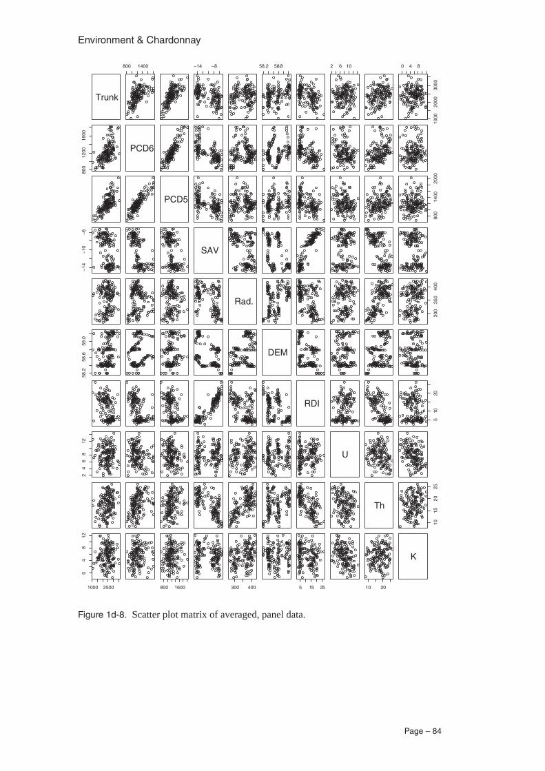
Environment & Chardonnay
Page – 84
Trunk
800 1400 −14 −8 58.2 58.8 2 6 10 0 4 8
1000
2000
3000
800
1200
1600
PCD6
PCD5
800
1400
2000
−14
−10
−6
SAV
Rad.
300
350
400
58.2
58.6
59.0
DEM
RDI
510
20
24
68
12
U
Th
1015
2025
1000 2500
04
812
800 1600 300 400 5 15 25 10 20
K
Figure 1d-8. Scatter plot matrix of averaged, panel data.
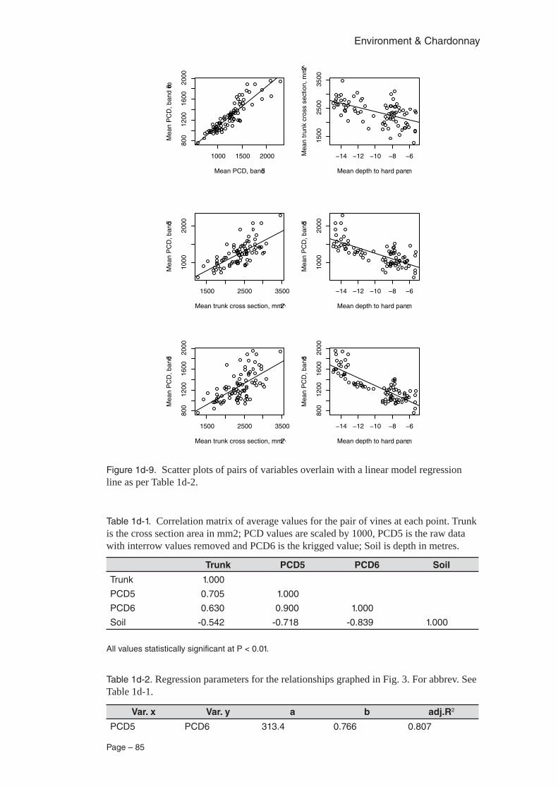
Page – 85
Environment & Chardonnay
1000 1500 2000
800
1200
1600
2000
Mean PCD, band 5M
ean
PC
D, b
and
6,
m
−14 −12 −10 −8 −6
1500
2500
3500
Mean depth to hard pan, m
Mea
n tr
unk
cros
s se
ctio
n, m
m2̂
1500 2500 3500
1000
2000
Mean trunk cross section, mm2̂
Mea
n P
CD
, ban
d 5
−14 −12 −10 −8 −6
1000
2000
Mean depth to hard pan, mM
ean
PC
D, b
and 5
1500 2500 3500
800
1200
1600
2000
Mean trunk cross section, mm2̂
Mea
n P
CD
, ban
d 6
−14 −12 −10 −8 −6
800
1200
1600
2000
Mean depth to hard pan, m
Mea
n P
CD
, ban
d 6
Figure 1d-9. Scatter plots of pairs of variables overlain with a linear model regression line as per Table 1d-2.
Table 1d-1. Correlation matrix of average values for the pair of vines at each point. Trunk is the cross section area in mm2; PCD values are scaled by 1000, PCD5 is the raw data with interrow values removed and PCD6 is the krigged value; Soil is depth in metres.
Trunk PCD5 PCD6 Soil
Trunk 1.000
PCD5 0.705 1.000
PCD6 0.630 0.900 1.000
Soil -0.542 -0.718 -0.839 1.000
All values statistically significant at P < 0.01.
Table 1d-2. Regression parameters for the relationships graphed in Fig. 3. For abbrev. See Table 1d-1.
Var. x Var. y a b adj.R2
PCD5 PCD6 313.4 0.766 0.807
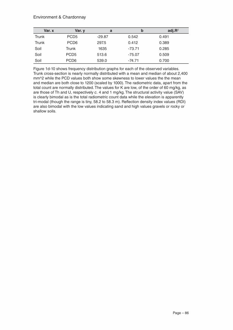
Environment & Chardonnay
Page – 86
Var. x Var. y a b adj.R2
Trunk PCD5 -29.87 0.542 0.491
Trunk PCD6 297.5 0.412 0.389
Soil Trunk 1635 -73.71 0.285
Soil PCD5 513.6 -75.07 0.509
Soil PCD6 539.0 -74.71 0.700
Figure 1d-10 shows frequency distribution graphs for each of the observed variables. Trunk cross-section is nearly normally distributed with a mean and median of about 2,400 mm^2 while the PCD values both show some skewness to lower values the the mean and median are both close to 1200 (scaled by 1000). The radiometric data, apart from the total count are normally distributed. The values for K are low, of the order of 60 mg/kg, as are those of Th and U, respectively c. 4 and 1 mg/kg. The structural activity value (SAV) is clearly bimodal as is the total radiometric count data while the elevation is apparently tri-modal (though the range is tiny, 58.2 to 58.3 m). Reflection density index values (RDI) are also bimodal with the low values indicating sand and high values gravels or rocky or shallow soils.
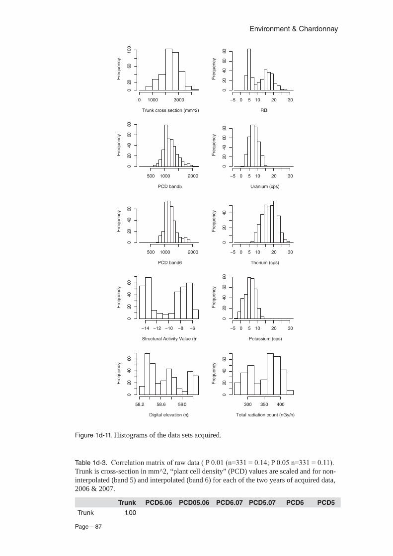
Page – 87
Environment & Chardonnay
Trunk cross section (mm^2)
Fre
quen
cy
0 1000 3000
020
6010
0
PCD band5
Fre
quen
cy
500 1000 2000
020
4060
80
PCD band6
Fre
quen
cy
500 1000 2000
020
4060
Structural Activity Value (m)
Fre
quen
cy
−14 −12 −10 −8 −6
020
4060
Digital elevation (m)
Fre
quen
cy
58.2 58.6 59.0
020
4060
RDI
Fre
quen
cy
−5 0 5 10 20 30
020
4060
80
Uranium (cps)
Fre
quen
cy
−5 0 5 10 20 30
020
4060
80
Thorium (cps)
Fre
quen
cy
−5 0 5 10 20 30
020
40
Potassium (cps)
Fre
quen
cy
−5 0 5 10 20 30
020
4060
80
Total radiation count (nGy/h)
Fre
quen
cy
300 350 400
020
4060
Figure 1d-11. Histograms of the data sets acquired.
Table 1d-3. Correlation matrix of raw data ( P 0.01 (n=331 = 0.14; P 0.05 n=331 = 0.11). Trunk is cross-section in mm^2, “plant cell density” (PCD) values are scaled and for non-interpolated (band 5) and interpolated (band 6) for each of the two years of acquired data, 2006 & 2007.
Trunk PCD6.06 PCD05.06 PCD6.07 PCD5.07 PCD6 PCD5
Trunk 1.00
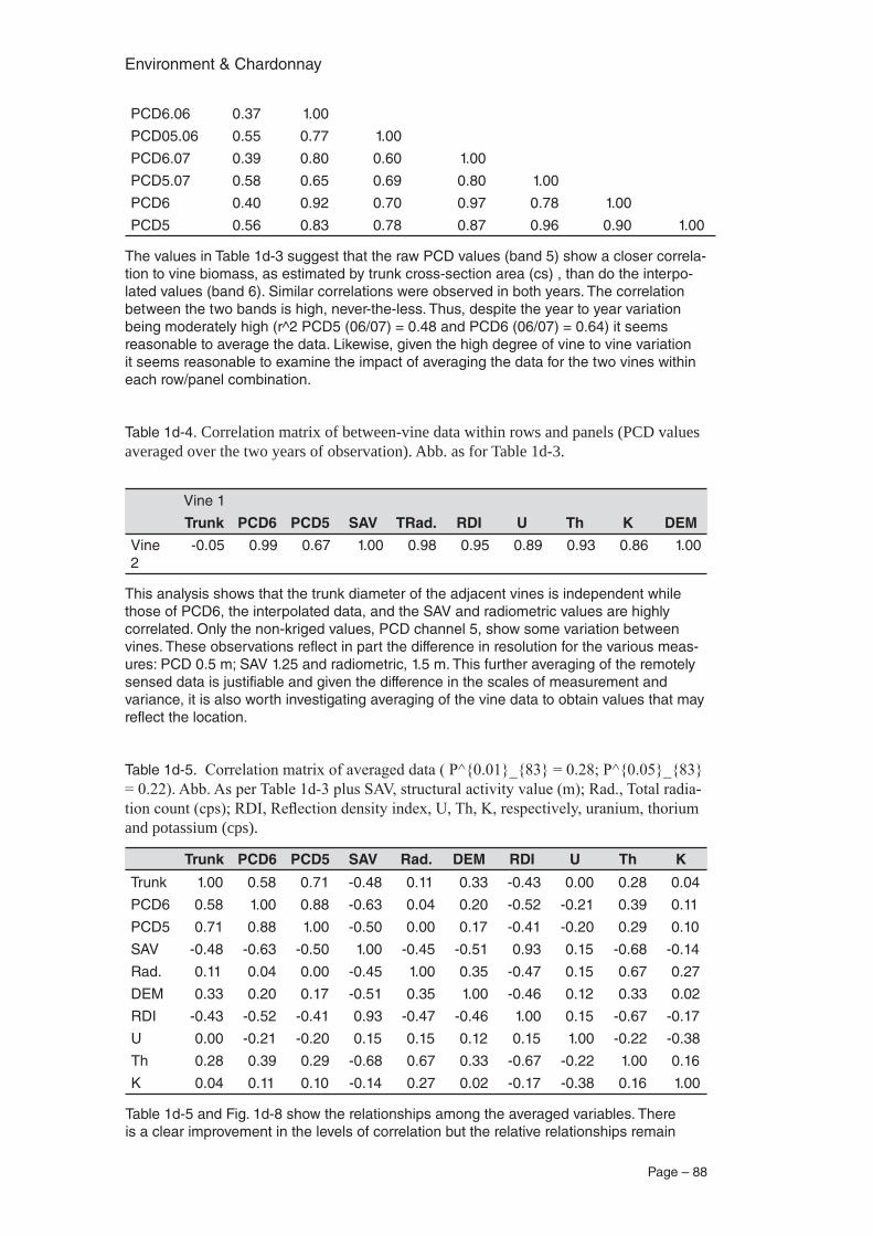
Environment & Chardonnay
Page – 88
PCD6.06 0.37 1.00
PCD05.06 0.55 0.77 1.00
PCD6.07 0.39 0.80 0.60 1.00
PCD5.07 0.58 0.65 0.69 0.80 1.00
PCD6 0.40 0.92 0.70 0.97 0.78 1.00
PCD5 0.56 0.83 0.78 0.87 0.96 0.90 1.00
The values in Table 1d-3 suggest that the raw PCD values (band 5) show a closer correla-tion to vine biomass, as estimated by trunk cross-section area (cs) , than do the interpo-lated values (band 6). Similar correlations were observed in both years. The correlation between the two bands is high, never-the-less. Thus, despite the year to year variation being moderately high (r^2 PCD5 (06/07) = 0.48 and PCD6 (06/07) = 0.64) it seems reasonable to average the data. Likewise, given the high degree of vine to vine variation it seems reasonable to examine the impact of averaging the data for the two vines within each row/panel combination.
Table 1d-4. Correlation matrix of between-vine data within rows and panels (PCD values averaged over the two years of observation). Abb. as for Table 1d-3.
Vine 1
Trunk PCD6 PCD5 SAV TRad. RDI U Th K DEM
Vine 2
-0.05 0.99 0.67 1.00 0.98 0.95 0.89 0.93 0.86 1.00
This analysis shows that the trunk diameter of the adjacent vines is independent while those of PCD6, the interpolated data, and the SAV and radiometric values are highly correlated. Only the non-kriged values, PCD channel 5, show some variation between vines. These observations reflect in part the difference in resolution for the various meas-ures: PCD 0.5 m; SAV 1.25 and radiometric, 1.5 m. This further averaging of the remotely sensed data is justifiable and given the difference in the scales of measurement and variance, it is also worth investigating averaging of the vine data to obtain values that may reflect the location.
Table 1d-5. Correlation matrix of averaged data ( P^{0.01}_{83} = 0.28; P^{0.05}_{83} = 0.22). Abb. As per Table 1d-3 plus SAV, structural activity value (m); Rad., Total radia-tion count (cps); RDI, Reflection density index, U, Th, K, respectively, uranium, thorium and potassium (cps).
Trunk PCD6 PCD5 SAV Rad. DEM RDI U Th K
Trunk 1.00 0.58 0.71 -0.48 0.11 0.33 -0.43 0.00 0.28 0.04
PCD6 0.58 1.00 0.88 -0.63 0.04 0.20 -0.52 -0.21 0.39 0.11
PCD5 0.71 0.88 1.00 -0.50 0.00 0.17 -0.41 -0.20 0.29 0.10
SAV -0.48 -0.63 -0.50 1.00 -0.45 -0.51 0.93 0.15 -0.68 -0.14
Rad. 0.11 0.04 0.00 -0.45 1.00 0.35 -0.47 0.15 0.67 0.27
DEM 0.33 0.20 0.17 -0.51 0.35 1.00 -0.46 0.12 0.33 0.02
RDI -0.43 -0.52 -0.41 0.93 -0.47 -0.46 1.00 0.15 -0.67 -0.17
U 0.00 -0.21 -0.20 0.15 0.15 0.12 0.15 1.00 -0.22 -0.38
Th 0.28 0.39 0.29 -0.68 0.67 0.33 -0.67 -0.22 1.00 0.16
K 0.04 0.11 0.10 -0.14 0.27 0.02 -0.17 -0.38 0.16 1.00
Table 1d-5 and Fig. 1d-8 show the relationships among the averaged variables. There is a clear improvement in the levels of correlation but the relative relationships remain
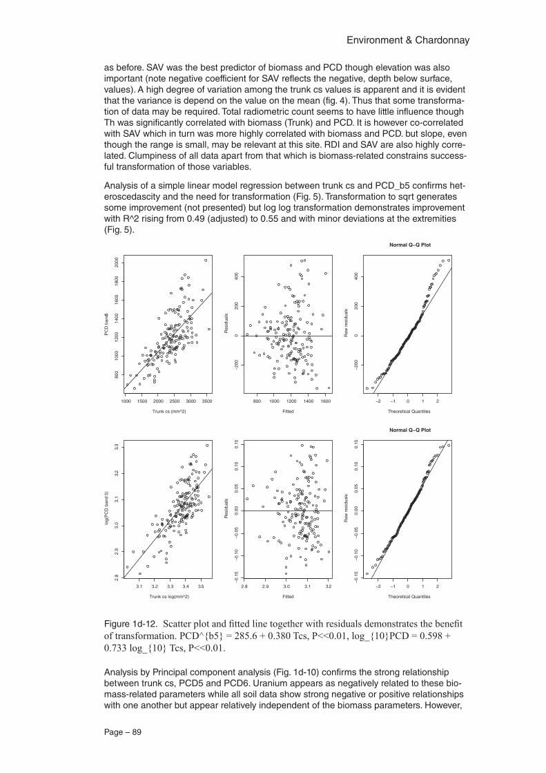
Page – 89
Environment & Chardonnay
as before. SAV was the best predictor of biomass and PCD though elevation was also important (note negative coefficient for SAV reflects the negative, depth below surface, values). A high degree of variation among the trunk cs values is apparent and it is evident that the variance is depend on the value on the mean (fig. 4). Thus that some transforma-tion of data may be required. Total radiometric count seems to have little influence though Th was significantly correlated with biomass (Trunk) and PCD. It is however co-correlated with SAV which in turn was more highly correlated with biomass and PCD. but slope, even though the range is small, may be relevant at this site. RDI and SAV are also highly corre-lated. Clumpiness of all data apart from that which is biomass-related constrains success-ful transformation of those variables.
Analysis of a simple linear model regression between trunk cs and PCD_b5 confirms het-eroscedascity and the need for transformation (Fig. 5). Transformation to sqrt generates some improvement (not presented) but log log transformation demonstrates improvement with R^2 rising from 0.49 (adjusted) to 0.55 and with minor deviations at the extremities (Fig. 5).
1000 1500 2000 2500 3000 3500
800
1000
1200
1400
1600
1800
2000
Trunk cs (mm^2)
PC
D b
and 5
800 1000 1200 1400 1600
−20
00
200
400
Fitted
Res
idua
ls
−2 −1 0 1 2
−20
00
200
400
Normal Q−Q Plot
Theoretical Quantiles
Raw
res
idua
ls
3.1 3.2 3.3 3.4 3.5
2.8
2.9
3.0
3.1
3.2
3.3
Trunk cs log(mm^2)
log(
PC
D b
and
5)
2.8 2.9 3.0 3.1 3.2
−0.
15−
0.10
−0.
050.
000.
050.
100.
15
Fitted
Res
idua
ls
−2 −1 0 1 2
−0.
15−
0.10
−0.
050.
000.
050.
100.
15
Normal Q−Q Plot
Theoretical Quantiles
Raw
res
idua
ls
Figure 1d-12. Scatter plot and fitted line together with residuals demonstrates the benefit of transformation. PCD^{b5} = 285.6 + 0.380 Tcs, P<<0.01, log_{10}PCD = 0.598 + 0.733 log_{10} Tcs, P<<0.01.
Analysis by Principal component analysis (Fig. 1d-10) confirms the strong relationship between trunk cs, PCD5 and PCD6. Uranium appears as negatively related to these bio-mass-related parameters while all soil data show strong negative or positive relationships with one another but appear relatively independent of the biomass parameters. However,
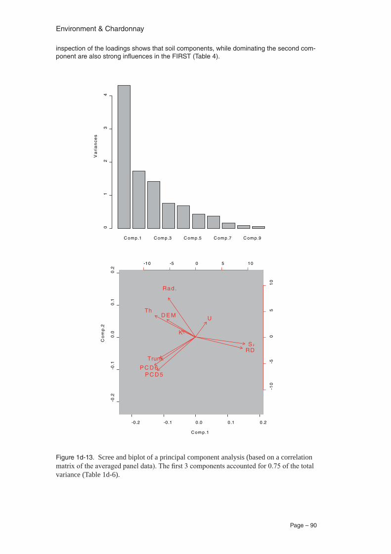
Environment & Chardonnay
Page – 90
inspection of the loadings shows that soil components, while dominating the second com-ponent are also strong influences in the FIRST (Table 4).
-0.2 -0.1 0.0 0.1 0.2
-0.2
-0.1
0.0
0.1
0.2
C omp.1
Co
mp
.2
1
2
3
45
6
7
8
910
11
1213
14
15
1617
18
19
20
21
222324
25
26
27
28
29
30
313233
34
35
36
37
38
39
4041
42
43
4445
46
47
48
49
50
5152
5354
555657
58
59
60
61
62
63
64
65
66
67
68
69
70
7172
73
74
75
76
77
78
79
80
81
82
83
84
85
86
87
88
899091
92
9394
95
96
97
98
99
100101102103104
105
106
107
108
109
110
111112113
114115116
117
118
119
120
121
122
123
124125
126127
128129
130
131
132
133 134
135
136
137
138
139
140
141142
143
144145
146
147
148149
150
151152
153
154
155
156
157
158
159
160161162
163
164165
166
167
168
-10 -5 0 5 10
-10
-50
51
0
Trunk
P C D 6P C D 5
Rad.
D E M
RD
UTh
K
S A
C omp.1 C omp.3 C omp.5 C omp.7 C omp.9
Va
ria
nc
es
01
23
4
Figure 1d-13. Scree and biplot of a principal component analysis (based on a correlation matrix of the averaged panel data). The first 3 components accounted for 0.75 of the total variance (Table 1d-6).
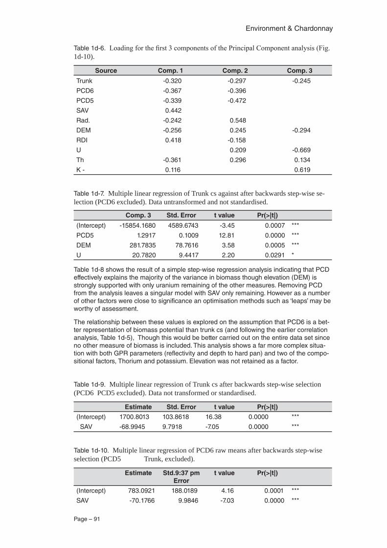
Page – 91
Environment & Chardonnay
Table 1d-6. Loading for the first 3 components of the Principal Component analysis (Fig. 1d-10).
Source Comp. 1 Comp. 2 Comp. 3
Trunk -0.320 -0.297 -0.245
PCD6 -0.367 -0.396
PCD5 -0.339 -0.472
SAV 0.442
Rad. -0.242 0.548
DEM -0.256 0.245 -0.294
RDI 0.418 -0.158
U 0.209 -0.669
Th -0.361 0.296 0.134
K - 0.116 0.619
Table 1d-7. Multiple linear regression of Trunk cs against after backwards step-wise se-lection (PCD6 excluded). Data untransformed and not standardised.
Comp. 3 Std. Error t value Pr(>|t|)
(Intercept) -15854.1680 4589.6743 -3.45 0.0007 ***
PCD5 1.2917 0.1009 12.81 0.0000 ***
DEM 281.7835 78.7616 3.58 0.0005 ***
U 20.7820 9.4417 2.20 0.0291 *
Table 1d-8 shows the result of a simple step-wise regression analysis indicating that PCD effectively explains the majority of the variance in biomass though elevation (DEM) is strongly supported with only uranium remaining of the other measures. Removing PCD from the analysis leaves a singular model with SAV only remaining. However as a number of other factors were close to significance an optimisation methods such as ‘leaps’ may be worthy of assessment.
The relationship between these values is explored on the assumption that PCD6 is a bet-ter representation of biomass potential than trunk cs (and following the earlier correlation analysis, Table 1d-5), Though this would be better carried out on the entire data set since no other measure of biomass is included. This analysis shows a far more complex situa-tion with both GPR parameters (reflectivity and depth to hard pan) and two of the compo-sitional factors, Thorium and potassium. Elevation was not retained as a factor.
Table 1d-9. Multiple linear regression of Trunk cs after backwards step-wise selection (PCD6 PCD5 excluded). Data not transformed or standardised.
Estimate Std. Error t value Pr(>|t|)
(Intercept) 1700.8013 103.8618 16.38 0.0000 ***
SAV -68.9945 9.7918 -7.05 0.0000 ***
Table 1d-10. Multiple linear regression of PCD6 raw means after backwards step-wise selection (PCD5 Trunk, excluded).
Estimate Std.9:37 pm Error
t value Pr(>|t|)
(Intercept) 783.0921 188.0189 4.16 0.0001 ***
SAV -70.1766 9.9846 -7.03 0.0000 ***
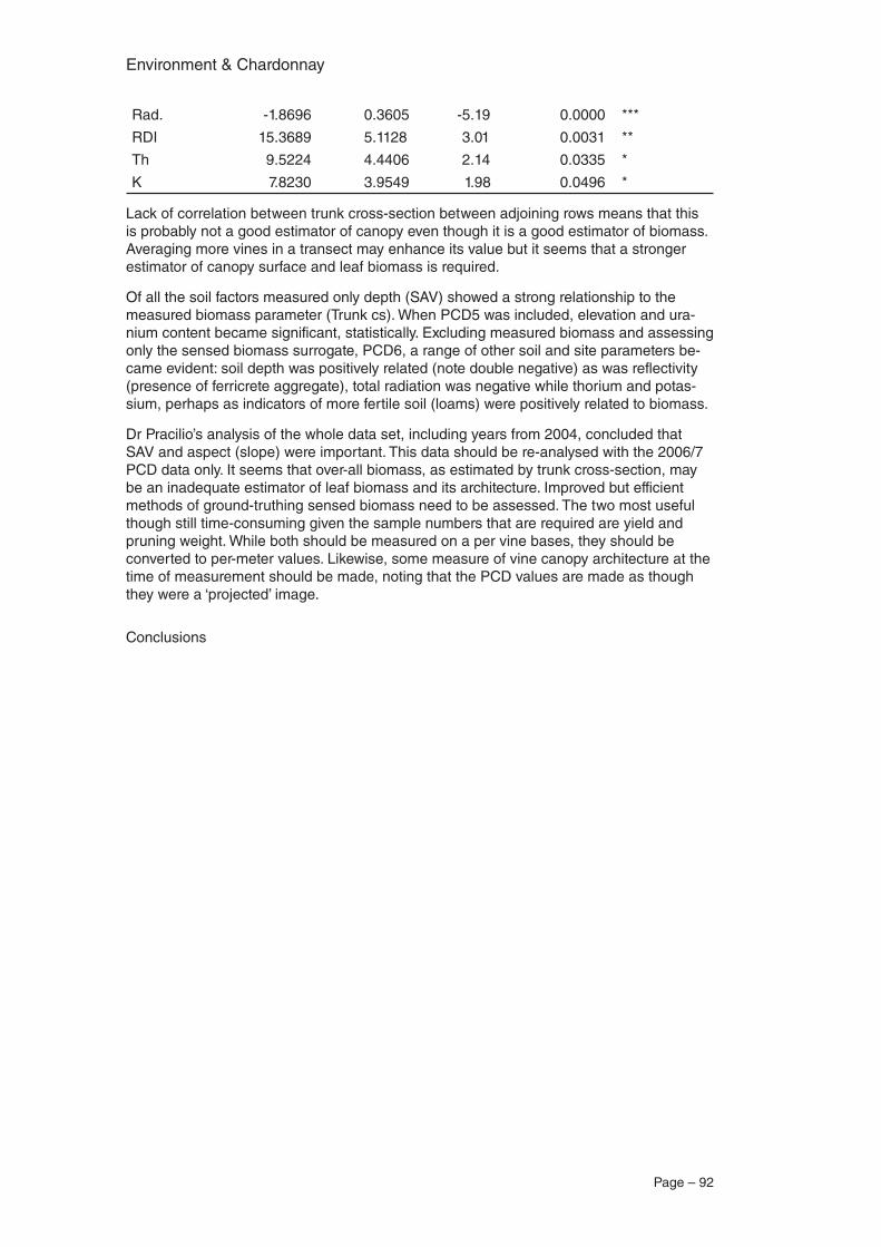
Environment & Chardonnay
Page – 92
Rad. -1.8696 0.3605 -5.19 0.0000 ***
RDI 15.3689 5.1128 3.01 0.0031 **
Th 9.5224 4.4406 2.14 0.0335 *
K 7.8230 3.9549 1.98 0.0496 *
Lack of correlation between trunk cross-section between adjoining rows means that this is probably not a good estimator of canopy even though it is a good estimator of biomass. Averaging more vines in a transect may enhance its value but it seems that a stronger estimator of canopy surface and leaf biomass is required.
Of all the soil factors measured only depth (SAV) showed a strong relationship to the measured biomass parameter (Trunk cs). When PCD5 was included, elevation and ura-nium content became significant, statistically. Excluding measured biomass and assessing only the sensed biomass surrogate, PCD6, a range of other soil and site parameters be-came evident: soil depth was positively related (note double negative) as was reflectivity (presence of ferricrete aggregate), total radiation was negative while thorium and potas-sium, perhaps as indicators of more fertile soil (loams) were positively related to biomass.
Dr Pracilio’s analysis of the whole data set, including years from 2004, concluded that SAV and aspect (slope) were important. This data should be re-analysed with the 2006/7 PCD data only. It seems that over-all biomass, as estimated by trunk cross-section, may be an inadequate estimator of leaf biomass and its architecture. Improved but efficient methods of ground-truthing sensed biomass need to be assessed. The two most useful though still time-consuming given the sample numbers that are required are yield and pruning weight. While both should be measured on a per vine bases, they should be converted to per-meter values. Likewise, some measure of vine canopy architecture at the time of measurement should be made, noting that the PCD values are made as though they were a ‘projected’ image.
Conclusions
Page – 93
Environment & Chardonnay
Modelling Meso-Climate in Margaret River: the Past and the Prospects under a 1.5x CO2
scenario‡.
Tom J. Lyons, School of Environmental Science, Murdoch University
John A. Considine, School of Plant Biology, UWA
Abstract
Temperature records for the Margaret River region are sparse and the impact of topogra-phy and distance from the coast is poorly understood. We have undertaken a modelling approach using the SCIRO TAPM model to estimate the climate from 1948 to the present. The model was validated by comparing predicted values against local weather station records. The modelling shows the strong impact of topography and especially of proxim-ity to the coast. The gradients being primarily from the coast inland though in summer there is stronger south-west - north-east gradient. Inclusion of a climate-change scenario demonstrates that while the general patterns will remain, less chilling, fewer optimal growing hours and more extreme temperature events may be anticipated. Interestingly, atmospheric saturation deficit is predicted to reduce, possibly due to increased summer rainfall events. However the changes are not so extreme that they will lead to a collapse of the industry. There may well be a need however to develop methods for managing dormancy in coastal sites and perhaps changing in time to cultivars better suited to a somewhat warmer climate.
IntroductionUnderstanding climate is integral to sustaining and strengthening the wine industry. Two of the three worrisome issues facing the Australian wine industry are climate related (climate change and water security; the other is marketing). Weather, today’s climate, is probably the issue that is uppermost in the practising viticulturist’s day- to-day thinking (vine-weather-yield-quality-pest and disease interactions). Climate is one of two fundamental considerations in site selection for wine producing vineyards (climate in relation to cultivar/quality/style choices and local site specific factors).
Climatic analysis also was used by John Gladstones to assist in identifying the potential of the Margaret River region in the early 1960’s, and by Harold Olmo in the mid-1950’s to identify locations in the ‘Great Southern’. Both regions have proven to consistently produce premium wines with regional mean $ / L values that are inspirational to other regions. The wonder of this is that Harold and John were able to achieve such success with scant records and by applying highly averaged data (mean monthly temperatures. It was up to the individ-ual grower however to determine how best to use this information with respect to actual site selection: this is a good region, where should I put my vineyard? Analysis of topography and the mesoclime can inform this process and thus take their pioneering work a step further.
The ProblemHowever, short time series and limited site specific data remain of concern even though we now have another 40 to 50 years of data since Olmo’s and Gladstones’ pioneering stud-ies. As a part of the ARC-Evans and Tate Wines Chardonnay research project we have established and accessed a spatially richer data set of local weather conditions through the installation of automatic weather stations on eleven sites. We also had access to records from other stations in the region managed by Agrilink International. However even this data set, though richer in the density of sampling within the region, is of limited duration – we can’t discern trends and we can’t judge how representative each year of our sampling was of the
‡Modified from an article that appeared in the Australian Grapegrower and Winemaker in 2007 (524) 65-69.
Environment & Chardonnay
Page – 94
‘population’ of years. Climate is notoriously variable and the last two years seemed par-ticularly extreme. So we sought to investigate whether climate modelling techniques could help to provide a sense of historical perspective.
The MethodWe applied modelling techniques akin to those used by national bureaus of meteorol-ogy to map and forecast weather and climate at a landscape scale. We sought however to refine this to a local scale and to provide climate (and even daily weather) records for individual localities, both historically and prospectively. For an excellent introduction to terminology we refer you to the Bureau of Meteorology (http://www.bom.gov.au/lam/).
Local climate is determined by the interaction between local and regional geography and regional climatic conditions. This is frequently termed ‘meso-climate’ or ‘topo-climate’ – ‘topo-’ because the influence of land form and aspect but also vegetation cover, soil type and the proximity of significant bodies of water, lakes and oceans. An appreciation of ‘topoclimate’ is essential in choosing appropriate sites for vineyards, especially in cool climate localities but also in optimally allocating cultivars to sites in even warmer climates such as Margaret River. It is also possible to modify meso- and micro-climate by practices such as the use of wind-breaks, cover crops and training practices.
In this study, we adapted software developed by CSIRO for predicting distribution of airborne pollutants [TAPM (Hurley, 2002)]. The large scale synoptic data required to initialize the model was extracted from the NCEP/NCAR reanalysis data provided by the NOAA-CIRES Climate Diagnostics Centre, Boulder, Colorado (http://www.cdc.noaa.gov/), climatological average ocean surface temperatures were obtained from the US National Centre for Atmospheric Research (http://dss.ucar.edu/catalogs/oceanlists/ocean.html), terrain height data at approximately 0.3 km spacing were obtained from Geoscience Australia (http://www. ga.gov.au) and local vegetation and soil type data at a resolution of approximately 5 km were obtained from CSIRO Wildlife and Ecology.
While the output of the model can be run on a desktop computer, running it for a region and for a large number of years required access to a super computer. The model was run on a 1.1 x 1.1 km grid and thus some of the finer-scale geographical features are lost. Never-the-less, the output seems reasonable, even though preliminary at this point. Also we discarded all but the land surface predictions to reduce the output to a manageable level.
The ResultsAs a first step we checked the model against local data and this gave us encouragement to continue (Figs 2-1A & B). These graphs show a comparison between hourly recorded values at the Vasse meteorological station of the Department of Agriculture and Food compared to the simultaneous model values at the nearest grid point. While there was significant scatter indicating that factors (i.e. local site effects , instrumental errors and deviations from climatological average sea surface temperatures) other than those used in the model affect the recorded temperature, the majority of values lie within +/- 2.3 ºC of the recorded value. Each of the predictions however carries this error which may have arisen either from the site recording process or from limitations of the model. Figure 2-1B shows that the model tends to under-estimate higher temperatures. We will incorporate more sites in the analysis in the future to give a greater understanding of the errors and whether they are spatially constant.
Regional climatic differences were assessed using this model. For example Figure 2-3A shows a map of the average hours of temperature that fall within the optimal values for vine growth for the years 1946 to 2005. Important gradients in temperature occur along the coast with some ‘islands’ of low temperatures inland. However two of these sites oc-cur close to the coast towards the southern end of the region. This distribution may be compared with the topographical map (Figure 2-2).
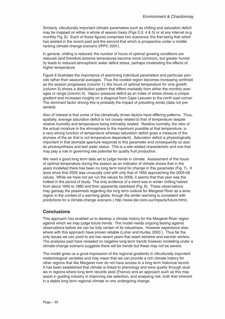
Page – 95
Environment & Chardonnay
Similarly, viticulturally important climatic parameters such as chilling and saturation deficit may be mapped on either a whole of season basis (Figs 2-3, 4 & 5) or at any interval (e.g. monthly Fig. 6). Each of these figures comprises two scenarios; the first being that which has existed in the recent past and the second that which is prospective under a middle ranking climate-change scenario (IPPC 2001).
In general, chilling is reduced, the number of hours of optimal growing conditions are reduced (and therefore extreme temeratures become more common), but greater humid-ity leads to reduced atmospheric water deficit stress, perhaps moderating the effects of higher temperature.
Figure 6 illustrates the importance of examining individual parameters and particular peri-ods rather than seasonal averages. Thus the coolest region becomes increasing confined as the season progresses (column 1); the hours of optimal temperature for vine growth (column 3) shows a distribution pattern that differs markedly from either the monthly aver-ages or range (column 4). Vapour pressure deficit as an index of stress shows a unique gradient and increases roughly on a diagonal from Cape Leeuwin to the north east corner. The dominant factor driving this is probably the impact of prevailing winds (data not pre-sented).
Also of interest is that some of the climatically driven factors have differing patterns. Thus, spatially, average saturation deficit is not closely related to that of temperature despite relative humidity and temperature being intimately related. Relative humidity, the ratio of the actual moisture in the atmosphere to the maximum possible at that temperature, is a very strong function of temperature whereas saturation deficit gives a measure of the dryness of the air that is not temperature dependent). Saturation deficit is physiologically important in that stomatal aperture responds to this parameter and consequently so also do photosynthesis and leaf water status. This is a site-related characteristic and one that may play a role in governing site potential for quality fruit production.
We need a good long term data set to judge trends in climate. Assessment of the hours of optimal temperature during the season as an indicator of climate shows that in the years modelled there has been no long term trend for change in this parameter (Fig. 7). It does show that 2005 was unusually cold with only that of 1950 approaching the 2005-06 values. While we have not yet run the values for 2006, it seems that that year was the hottest in the period of study. The only evidence of a trend was in winter chilling halved from about 1950 to 1980 and then apparently stabilised (Fig. 8). These observations may gainsay the pessimists regarding the long term outlook for Margaret River as a wine region in the context of a warming globe, though the winter warming is consistent with predictions for a climate-change scenario ( http://www.dar.csiro.au/impacts/future.html).
ConclusionsThis approach has enabled us to develop a climate history for the Margaret River region against which we may judge future trends. The model needs ongoing testing against observations before we can be fully certain of its robustness. However experience else-where with this approach have proven reliable (Luhar and Hurley, 2003 ). Thus far the only issues we can point to are two recent years that seem extreme and warmer winters. The analyses past have revealed no negative long-term trends however modelling under a climate-change scenario suggests there will be trends but these may not be severe.
The model gives us a good impression of the regional gradients in viticulturally important meteorological variables and may mean that we can provide a rich climate history for other regions that like Margaret river do not have access to a long term historical record. It has been established that climate is linked to phenology and wine quality through stud-ies in regions where long term records exist (France) and an approach such as this may assist in guiding industry in improving site selection, and analysing risk, both that inherent in a stable long term regional climate or one undergoing change.
Environment & Chardonnay
Page – 96
ACKNOWLEDGEMENTSEvans & Tate Wine Company for financial and in-kind support; Agrilink International for the donation of weather stations and data acquisition support; Australian Research Council and Grape and Wine R&D corporation for financial support towards the weather station network and technical salaries; Interactive Virtual Environment Centre (iVEC) for ac-cess to supercomputing facilities and support, Department of Land Administration for the provision of topographical and vegetation cover maps and Anthony Robinson for technical support. We thank Peter Hurley CSIRO for assistance in recompiling TAPM to run on the iVEC
Bibliography & Further ReadingChuine I, Yiou P, Viovy N, Seguin B, Daux V, Ladurie EL (2004) Historical phenology: Grape ripening
as a past climate indicator. Nature 432, 289-290.
CSIRO Atmospheric Research Internal Paper No. 25, Aspendale, Victoria
Gladstones, J. (2004), Climate and Australian Viticulture. In, “Viticulture – V1 Resources” Eds Dry, PR and Coombe, B.G. Winetitles, Adelaide.
Hurley. P., 2002: The air pollution model (TAPM) version 2 User manual
IPCC (2001): Climate Change 2001: The Scientific Basis of Climate Change. Summary for Policy-makers. Intergovernmental Panel on Climate Change. www.unep.ch/ipcc
Jones GV, Davis RE (2000) Climate influences on grapevine phenology, grape composition, and wine production and quality for Bordeaux, France. American Journal of Enology and Viticulture 51, 249-261.
Luhar A.K.and Hurley P.J., 2003: Evaluation of TAPM, a prognostic meteorological and air pollution model, using urban and rural point-source data. Atmospheric Environment, 37, 2795-2810.
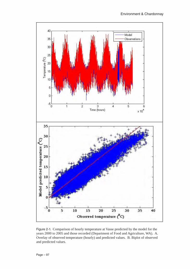
Page – 97
Environment & Chardonnay
Figure 2-1. Comparison of hourly temperature at Vasse predicted by the model for the years 2000 to 2005 and those recorded (Department of Food and Agriculture, WA). A. Overlay of observed temperature (hourly) and predicted values. B. Biplot of observed and predicted values.
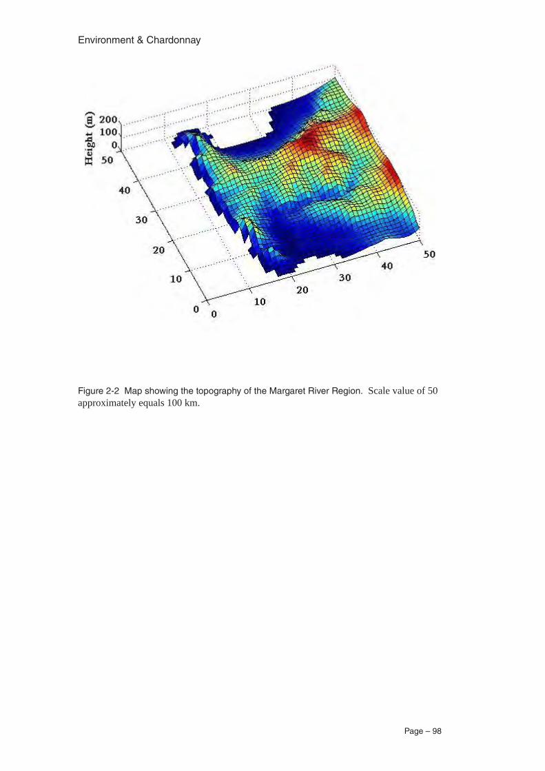
Environment & Chardonnay
Page – 98
Figure 2-2 Map showing the topography of the Margaret River Region. Scale value of 50 approximately equals 100 km.
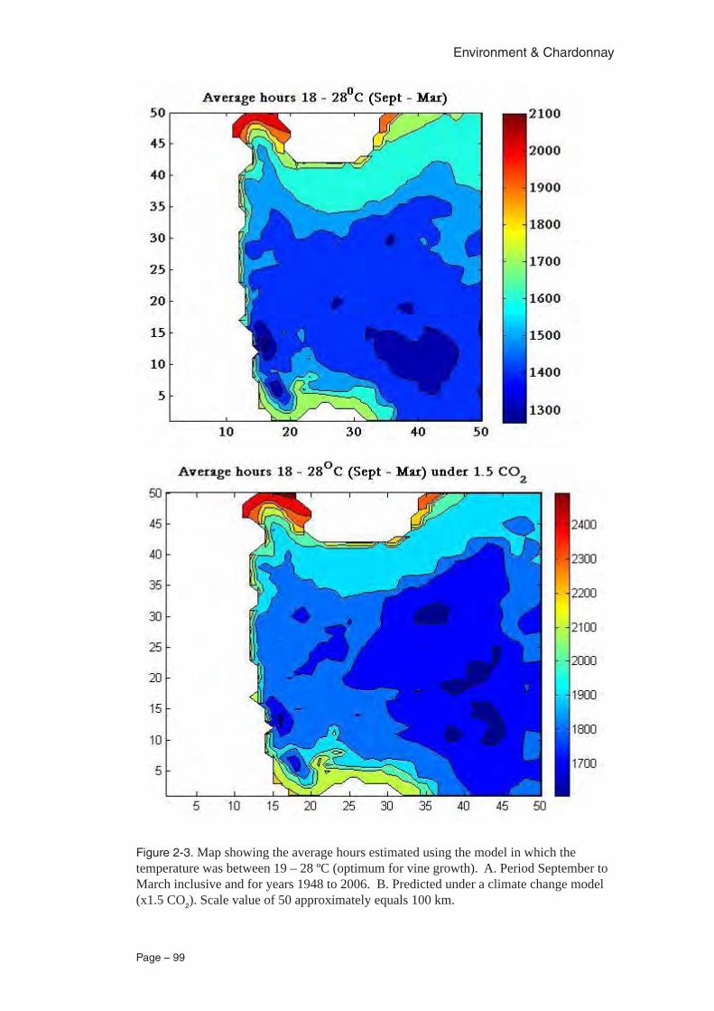
Page – 99
Environment & Chardonnay
Figure 2-3. Map showing the average hours estimated using the model in which the temperature was between 19 – 28 ºC (optimum for vine growth). A. Period September to March inclusive and for years 1948 to 2006. B. Predicted under a climate change model (x1.5 CO2). Scale value of 50 approximately equals 100 km.
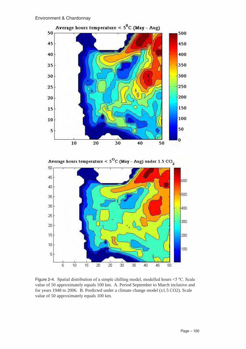
Environment & Chardonnay
Page – 100
Figure 2-4. Spatial distribution of a simple chilling model, modelled hours <5 ºC. Scale value of 50 approximately equals 100 km. A. Period September to March inclusive and for years 1948 to 2006. B. Predicted under a climate change model (x1.5 CO2). Scale value of 50 approximately equals 100 km.
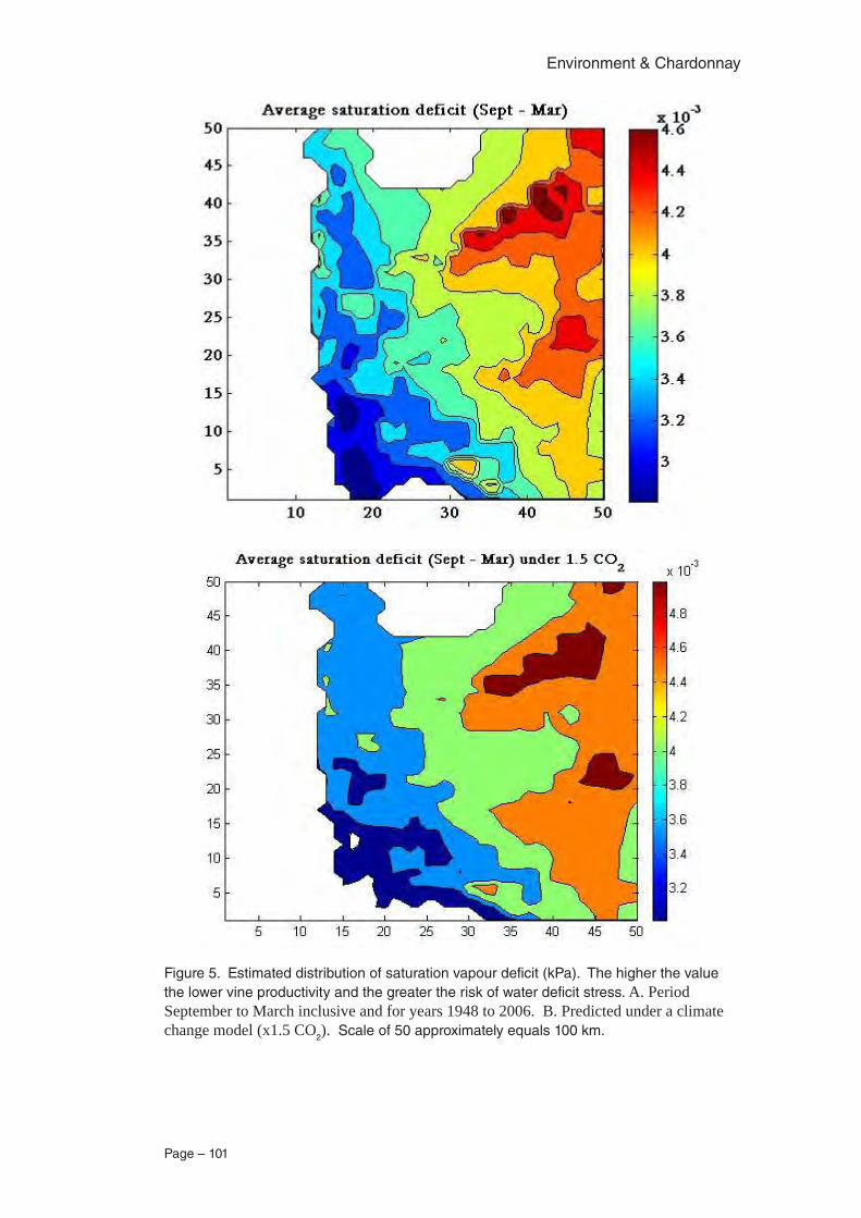
Page – 101
Environment & Chardonnay
Figure 5. Estimated distribution of saturation vapour deficit (kPa). The higher the value the lower vine productivity and the greater the risk of water deficit stress. A. Period September to March inclusive and for years 1948 to 2006. B. Predicted under a climate change model (x1.5 CO2). Scale of 50 approximately equals 100 km.
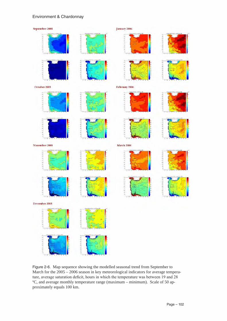
Environment & Chardonnay
Page – 102
Figure 2-6. Map sequence showing the modelled seasonal trend from September to March for the 2005 – 2006 season in key meteorological indicators for average tempera-ture, average saturation deficit, hours in which the temperature was between 19 and 28 ºC, and average monthly temperature range (maximum – minimum). Scale of 50 ap-proximately equals 100 km.
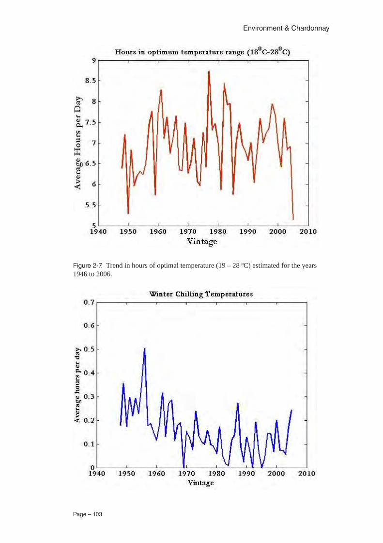
Page – 103
Environment & Chardonnay
Figure 2-7. Trend in hours of optimal temperature (19 – 28 ºC) estimated for the years 1946 to 2006.
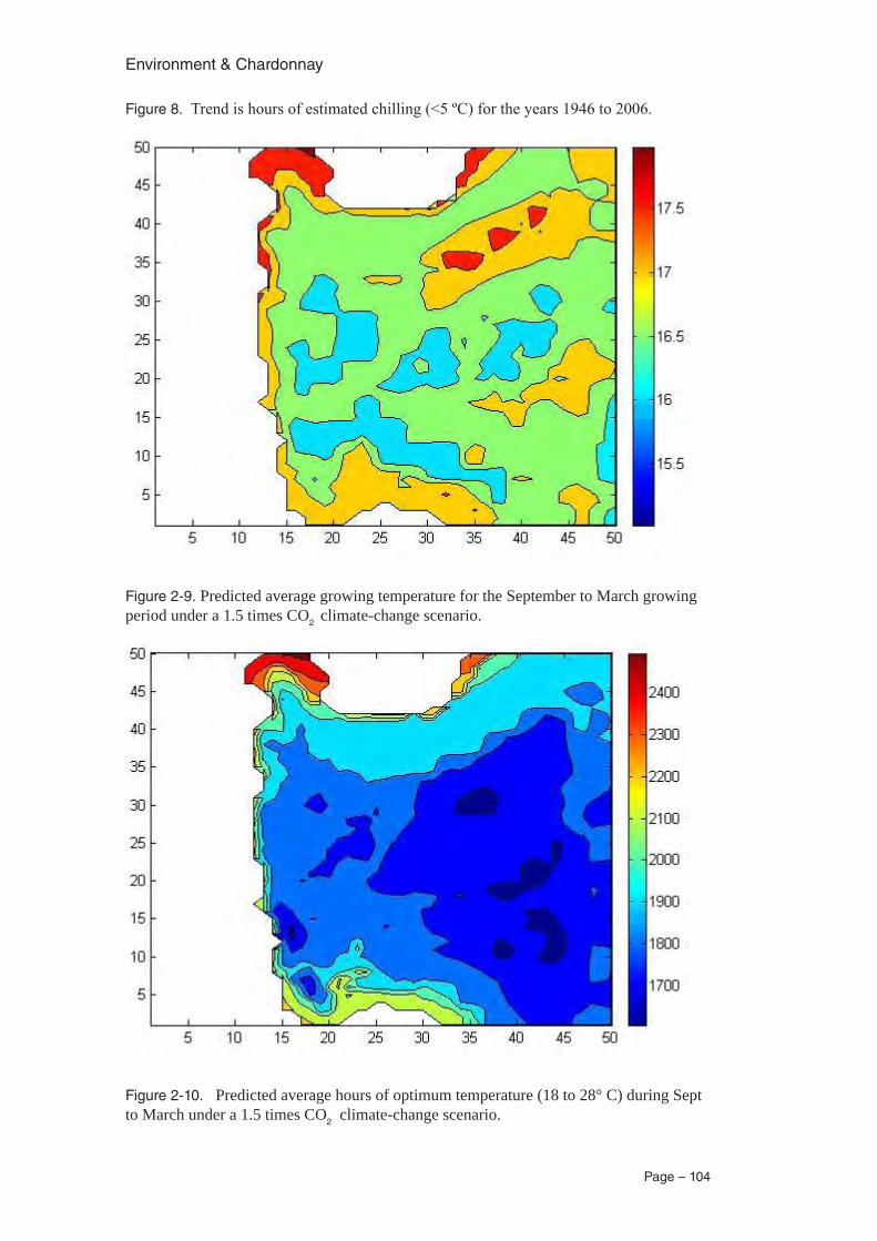
Environment & Chardonnay
Page – 104
Figure 8. Trend is hours of estimated chilling (<5 ºC) for the years 1946 to 2006.
Figure 2-9. Predicted average growing temperature for the September to March growing period under a 1.5 times CO2 climate-change scenario.
Figure 2-10. Predicted average hours of optimum temperature (18 to 28° C) during Sept to March under a 1.5 times CO2 climate-change scenario.
Page – 105
Environment & Chardonnay
Wine
Contributing authors: L. Francis, Belinda Bramley and Patricia Osidacz
Australian Wine Research Institute;
A. Robinson and J.A Considine, School of Plant Biology, UWA
Abstract
Small lot wines were made in triplicate from two plots located in each of 11 vineyards in the Margaret River Geographical Region with purpose of assess-ing location differences. The cultivar used was Chardonnay, clone ‘Gingin’. The process was conducted in each of three vintages, 2004 to 2006; the first was as-sessed in a formal but preliminary fashion, the second under formal conditions at the Australian Wine Research Institute and the third remains unassessed.
Variation in fermentation progress masked the sensory attributes of some of the wines in each year. Analysis of the data from 2005 showed that the differences in fermentation rate were related to site and thus are unlikely to have been primarily technical in nature. Despite this limitation there were indications that wines from vineyards in the upper Chapman Brook region possessed the most desirable sensory attributes. One in particular (cg10) was noteworthy in terms of fruity (passionfruit, grapefruit) and herbaceous characters. This wine has been selected for further analysis by AWRI. The remaining wines were generally neutral making distinction difficult, particularly in 2004.
IntroductionThere is good support for the concept, that site, soil, climate and geography influence the sensory properties and quality of the wine of individual cultivars (e.g. Gladstones 1992, Jones & Davis 2000, White 2003) while there is also considerable research that demon-strates the influence of management (e.g. Smart 1991). This research was undertaken to document the site characteristics and to explore their relationship to location and vine state (presented elsewhere). The sites were selected in consultation with staff of industry partner, Evans and Tate Wines Ltd and varied substantially in age and management but were regard-ed as all being of the one clone, Chardonnay ‘Gingin’. It was this clone that the fine reputa-tion for premium quality Chardonnay wines was developed in Margaret River (e.g. Leeuwin Estate, Cullens and Devil’s Lair). These vineyards were not included in the research as only those vineyards supplying fruit to the partner were included. Never-the-less, the sample represented the major sub-regions with the exclusion of the coastal region to the west of the town site (the location of Leeuwin and Voyager for example).
Materials & Methods
Chemistry
Brix was measured using a temperature compensated digital meter (Atago PAL-1™ ) while Baumé and ferment temperature with a digital, temperature compensated, density meter. (Anton Par DMA53n™). Both instruments were calibrated against deionised water and a su-crose standard (c. 18% w/w/). pH and titratable acids (in tartaric acid equivalents, g/L) were measured with an automatic burette (Metrohm Titrino 719S™). Sulphur dioxide was meas-ured by aspiration (Rankine 1970, Buechsenstein & Ough CS 1978) while fermentable amino acids were determined by colourimetry (Dukes & Butzke 1998). Ammonium was estimated by enzyme assay (Boerhinger™ or Arrow™ ). Residual sugar was estimated first by Clin-istix™ and confirmed by enzymatic assay (D-glucose/D-fructose enzyme kit, Boerhinger™
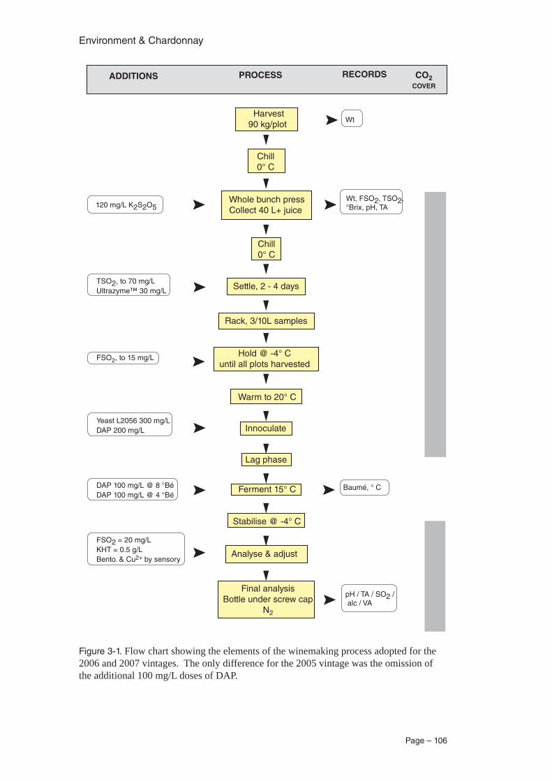
Environment & Chardonnay
Page – 106
Figure 3-1. Flow chart showing the elements of the winemaking process adopted for the 2006 and 2007 vintages. The only difference for the 2005 vintage was the omission of the additional 100 mg/L doses of DAP.
Wt
Wt, FSO2, TSO2,°Brix, pH, TA
Baumé, ° C
pH / TA / SO2 / alc / VA
PROCESS RECORDS CO2COVER
Harvest90 kg/plot
Chill0° C
Whole bunch pressCollect 40 L+ juice
Chill0° C
Settle, 2 - 4 days
Rack, 3/10L samples
Hold @ -4° Cuntil all plots harvested
Warm to 20° C
Innoculate
Lag phase
Ferment 15° C
Stabilise @ -4° C
Analyse & adjust
Final analysisBottle under screw cap
N2
ADDITIONS
120 mg/L K2S2O5
TSO2, to 70 mg/LUltrazyme™ 30 mg/L
FSO2, to 15 mg/L
Yeast L2056 300 mg/LDAP 200 mg/L
DAP 100 mg/L @ 8 °BéDAP 100 mg/L @ 4 °Bé
FSO2 = 20 mg/LKHT = 0.5 g/LBento. & Cu2+ by sensory
Page – 107
Environment & Chardonnay
or Arrow™) or in 2007 by a modified Somogyi-Nelson assay (Somogyi 1952, Fales et al. 1961, Considine unpublished).
Winemaking
The general process adopted is shown in Fig. 3.1. This was developed in consultation with the partner winemakers and staff of AWRI and Provisor.
Acid Targets:
All acid additions were of tartaric acid (TA) as required and dissolved in a minimum vol-ume of warm deionised (DI) water. Targets were as below but a TA level 9 g/L was set as an upper limit. No additions were made after cold settling.
Target pH
Pressing: 3.5 to 3.7
Juice: 3.20 to 3.50
Wine 3.35
SO2 Targets
All SO2 additions prepared from potassium metabisulphite (PMS, K2S205) equivalents of SO2 dissolved in a minimum volume of warm DI water. SO2 levels were checked before any wine movement and where necessary an addition of 10 mg/L was made to protect the wine/juice during the transfer activity.
Addition Target
Pressing: 70 mg/L SO2; 35 mg/L SO2 free
Juice: Adjust to 10-15 mg/L SO2 free
Preferment: 5-10 mg/L SO2 free
Post-Ferment: 40 mg/L SO2; 20 mg/L SO2 free
Wine: Adjust to 20 mg/L SO2 free
Pre-bottling: Adjust to 20 mg/L SO2 free
In bottle: 20 mg/L SO2 free
Diammonium Hydrogen Phosphate (DAP) Additions
DAP was added as required during fermentation up to a maximum of 500 mg/L total with no additions after 4° Bé. No single addition was larger than 100 mg/L to avoid unpredict-able fermentation activity. DAP was prepared in a minimum amount of warm DI water.
Copper Sulphate (CuSO4) Additions
Cu2+ was added as CuSO4 dissolved in a minimum amount of warm DI water to the equivalent of 100 g/L CuSO4. Copper fining was conducted under CO2 gas cover and the solution added in slow increments with agitation. This was added post fermentation with the SO2 addition and prior to bentonite fining. The rate of addition was determined in con-sultation with the industry partner but with an upper limit of 0.2 mg/L.
Heat and Cold Stabilization
Bentonite was prepared at least 12 hrs prior to addition in the proportions of 1 kg in 10 L hot filtered water with 10 g citric acid while stirring rapidly and held in a hot water bath set at 60° C. The rate of addition was determined in consultation with the industry partner who conducted a sensory evaluation. Bentonite was added to the wine under CO2 gas cover with significant agitation following addition of 0.5 g/L crème of tartar (KH2T).
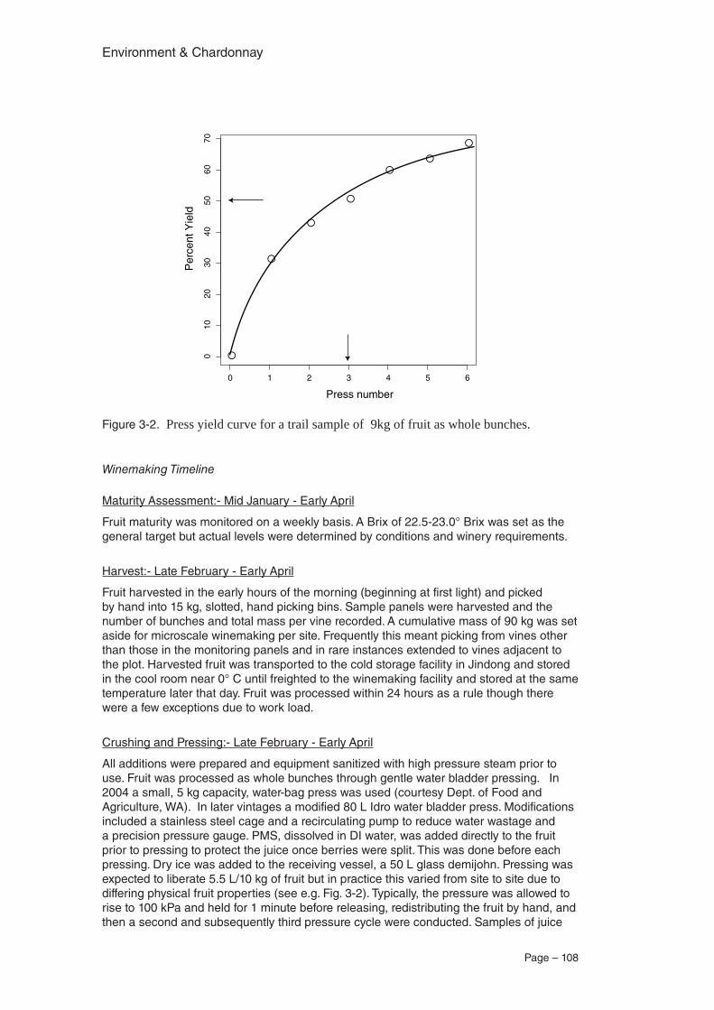
Environment & Chardonnay
Page – 108
Winemaking Timeline
Maturity Assessment:- Mid January - Early April
Fruit maturity was monitored on a weekly basis. A Brix of 22.5-23.0° Brix was set as the general target but actual levels were determined by conditions and winery requirements.
Harvest:- Late February - Early April
Fruit harvested in the early hours of the morning (beginning at first light) and picked by hand into 15 kg, slotted, hand picking bins. Sample panels were harvested and the number of bunches and total mass per vine recorded. A cumulative mass of 90 kg was set aside for microscale winemaking per site. Frequently this meant picking from vines other than those in the monitoring panels and in rare instances extended to vines adjacent to the plot. Harvested fruit was transported to the cold storage facility in Jindong and stored in the cool room near 0° C until freighted to the winemaking facility and stored at the same temperature later that day. Fruit was processed within 24 hours as a rule though there were a few exceptions due to work load.
Crushing and Pressing:- Late February - Early April
All additions were prepared and equipment sanitized with high pressure steam prior to use. Fruit was processed as whole bunches through gentle water bladder pressing. In 2004 a small, 5 kg capacity, water-bag press was used (courtesy Dept. of Food and Agriculture, WA). In later vintages a modified 80 L Idro water bladder press. Modifications included a stainless steel cage and a recirculating pump to reduce water wastage and a precision pressure gauge. PMS, dissolved in DI water, was added directly to the fruit prior to pressing to protect the juice once berries were split. This was done before each pressing. Dry ice was added to the receiving vessel, a 50 L glass demijohn. Pressing was expected to liberate 5.5 L/10 kg of fruit but in practice this varied from site to site due to differing physical fruit properties (see e.g. Fig. 3-2). Typically, the pressure was allowed to rise to 100 kPa and held for 1 minute before releasing, redistributing the fruit by hand, and then a second and subsequently third pressure cycle were conducted. Samples of juice
C
M
Y
CM
MY
CY
CMY
K
wine.A.2.pdf 15/04/09 9:15:08 PM
Figure 3-2. Press yield curve for a trail sample of 9kg of fruit as whole bunches.
Page – 109
Environment & Chardonnay
were taken at this point for mineral element, organic acid, and amino acid analysis. Pecti-nase was added under CO2 cover, sealed, and left in the 0° C room to settle for two days.
Racking and Storage:- Early March - Early April
Once settled, a sample of juice was analysed (pH, TA, SO2, Baumé) and additions (tartar-ic acid, SO2) were prepared. The juice was racked from the settling vessel into three 10 L glass demijohn fermentation vessels under CO2 cover, topped and sealed with a silicone rubber stopper. Juice was racked onto any required additions. The fermentation vessels were stored in the 0° C room prior to inoculation (1 to 5 weeks).
Fermentation:- Early April - Mid April
Yeast culture preparation [L2056 http://www.lallemandwine.us/products/yeast_chart.php] was done while juices were warming in a fermentation room set at 20° C. Small volumes of juice (~250 ml/10L ferment) were removed from the fermentation vessels to minimise volume losses and potential bacterial contamination from active ferment over-flows breaching air locks (containing 1% PMS). A 200 mg/L DAP addition was made prior to inoculation. The yeast inoculum was prepared in bulk for all ferments at a rate of 300 mg/L as per supplier instructions. Rehydration was conducted using Go-Ferm™ to aid in yeast sterol production. The inoculum was dosed under CO2 gas cover at a standard rate into each fermentation vessel. CO2 gas cover was maintained until active fermen-tation was observed. At this point the temperature was lowered progressively to 15° C over 48 hours. Fermentation rounds were conducted twice per day at ~12 hour intervals monitoring temperature and baumé, except at the beginning when three-times daily was required to ensure fermentation rate was controlled during the early log phase. Fermenta-tion was conducted at ~15° C but aimed for 1.0 baumé drop per day. When fermentation rate dropped below 0.8 Baumé per day the temperature was raised to ~18° C over a 24 hour period. Additional DAP additions were made uniformly to all ferments following the exponential growth phase. Leading up to the conclusion of fermentation CO2 gas cover should be maintained and once hydrometry readings fell below 0 Baumé clinitest tablets was used to determine dryness. This was confirmed by enzymatic assay for total reduc-ing sugars or by a modified Somogyi-Nelson assay (Considine unpublished). Once the ferment fell below 2 g/L the ferment was [protected with a CO2 gas cover, treated with an SO2 addition, chilled and sealed. End of fermentation analysis were carried out (pH, TA, reducing sugar, alcohol, VA, SO2) and any necessary acid/SO2 additions made. Wines were stored, post ferment, at -4° C to aid settling and cold stabilization. CO2 cover and SO2 levels maintained in completed ferments until all ferments were complete.
In 2005 sluggish ferments were treated by regular swirling to overcome flocculation and the addition of yeast hulls.
Stabilization:- Early May - Mid May
As bentonite has been noted to strip wines of flavour and common scientific practice has been to add a standard minimum level to achieve protein stability in microscale winemak-ing trials. As this was an industry related study, commercial levels of protein stability were determined by the industry partner laboratory. The bentonite addition and créme of tartar were added to each wine under CO2 cover following any copper fining, mixed, and left to settle at -4° C for 2 weeks. Once bentonite lees had settled, a sample was taken for analy-sis (SO2, pH, TA). The stable wine was racked under CO2 and SO2 adjusted immediately pre-bottling.
Bottling:- Mid May - Late May
All bottling equipment was sterilised and a screw cap applicator calibrated. Bottles were washed with hot water (80° C) and left to cool inverted prior to filling. Bottles were filled under nitrogen to allow a 30 mm head space and sealed with screw cap immediately, la-belled, and packed in wine cartons. All bottling materials were supplied by industry partner and were of appropriate quality for short to medium term storage.
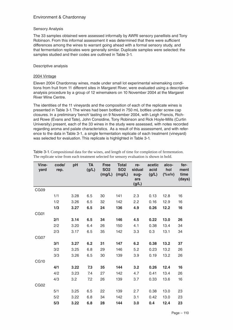
Environment & Chardonnay
Page – 110
Sensory Analysis
The 33 samples obtained were assessed informally by AWRI sensory panellists and Tony Robinson. From this informal assessment it was determined that there were sufficient differences among the wines to warrant going ahead with a formal sensory study, and that fermentation replicates were generally similar. Duplicate samples were selected: the samples studied and their codes are outlined in Table 3-1.
Descriptive analysis
2004 Vintage
Eleven 2004 Chardonnay wines, made under small lot experimental winemaking condi-tions from fruit from 11 different sites in Margaret River, were evaluated using a descriptive analysis procedure by a group of 12 winemakers on 10 November 2004 at the Margaret River Wine Centre.
The identities of the 11 vineyards and the composition of each of the replicate wines is presented in Table 3-1. The wines had been bottled in 750 mL bottles under screw cap closures. In a preliminary ‘bench’ tasting on 9 November 2004, with Leigh Francis, Rich-ard Rowe (Evans and Tate), John Considine, Tony Robinson and Rick Hoyle-Mills (Curtin University) present, each of the 33 wines in the study were assessed, with notes recorded regarding aroma and palate characteristics. As a result of this assessment, and with refer-ence to the data in Table 3-1, a single fermentation replicate of each treatment (vineyard) was selected for evaluation. This replicate is highlighted in Table 3-1.
Table 3-1. Compositional data for the wines, and length of time for completion of fermentation. The replicate wine from each treatment selected for sensory evaluation is shown in bold.
Vine-yard
code/ rep.
pH TA (g/L)
Free SO2
(mg/L)
Total SO2
(mg/L)
re-sidual sug-ars
(g/L)
acetic acid (g/L)
alco-hol
(%v/v)
fer-ment time
(days)
CG09
1/1 3.28 6.5 30 141 2.3 0.13 12.8 16
1/2 3.26 6.5 32 142 2.2 0.16 12.9 16
1/3 3.27 6.5 24 136 4.9 0.26 12.2 16
CG01
2/1 3.14 6.5 34 146 4.5 0.22 13.0 26
2/2 3.20 6.4 26 150 4.1 0.38 13.4 34
2/3 3.17 6.5 35 142 3.3 0.3 13.1 34
CG07
3/1 3.27 6.2 31 147 6.2 0.38 13.2 37
3/2 3.25 6.8 29 146 5.2 0.23 13.2 26
3/3 3.26 6.5 30 139 3.9 0.19 13.2 26
CG10
4/1 3.22 7.3 35 144 3.2 0.26 12.4 16
4/2 3.23 7.4 27 142 4.7 0.41 13.4 26
4/3 3.2 7.2 26 139 3.7 0.33 13.6 16
CG02
5/1 3.25 6.5 22 139 2.7 0.38 13.0 23
5/2 3.22 6.8 34 142 3.1 0.42 13.0 23
5/3 3.22 6.8 28 144 3.0 0.4 12.4 23
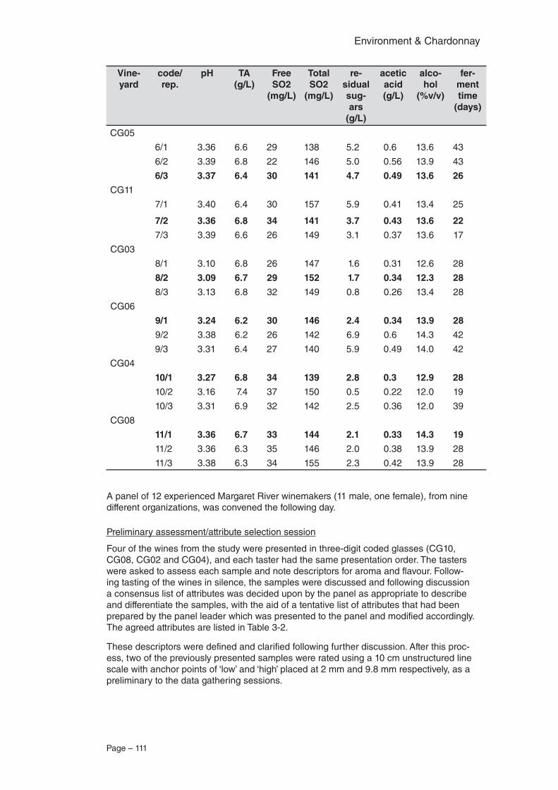
Page – 111
Environment & Chardonnay
Vine-yard
code/ rep.
pH TA (g/L)
Free SO2
(mg/L)
Total SO2
(mg/L)
re-sidual sug-ars
(g/L)
acetic acid (g/L)
alco-hol
(%v/v)
fer-ment time
(days)
CG05
6/1 3.36 6.6 29 138 5.2 0.6 13.6 43
6/2 3.39 6.8 22 146 5.0 0.56 13.9 43
6/3 3.37 6.4 30 141 4.7 0.49 13.6 26
CG11
7/1 3.40 6.4 30 157 5.9 0.41 13.4 25
7/2 3.36 6.8 34 141 3.7 0.43 13.6 22
7/3 3.39 6.6 26 149 3.1 0.37 13.6 17
CG03
8/1 3.10 6.8 26 147 1.6 0.31 12.6 28
8/2 3.09 6.7 29 152 1.7 0.34 12.3 28
8/3 3.13 6.8 32 149 0.8 0.26 13.4 28
CG06
9/1 3.24 6.2 30 146 2.4 0.34 13.9 28
9/2 3.38 6.2 26 142 6.9 0.6 14.3 42
9/3 3.31 6.4 27 140 5.9 0.49 14.0 42
CG04
10/1 3.27 6.8 34 139 2.8 0.3 12.9 28
10/2 3.16 7.4 37 150 0.5 0.22 12.0 19
10/3 3.31 6.9 32 142 2.5 0.36 12.0 39
CG08
11/1 3.36 6.7 33 144 2.1 0.33 14.3 19
11/2 3.36 6.3 35 146 2.0 0.38 13.9 28
11/3 3.38 6.3 34 155 2.3 0.42 13.9 28
A panel of 12 experienced Margaret River winemakers (11 male, one female), from nine different organizations, was convened the following day.
Preliminary assessment/attribute selection session
Four of the wines from the study were presented in three-digit coded glasses (CG10, CG08, CG02 and CG04), and each taster had the same presentation order. The tasters were asked to assess each sample and note descriptors for aroma and flavour. Follow-ing tasting of the wines in silence, the samples were discussed and following discussion a consensus list of attributes was decided upon by the panel as appropriate to describe and differentiate the samples, with the aid of a tentative list of attributes that had been prepared by the panel leader which was presented to the panel and modified accordingly. The agreed attributes are listed in Table 3-2.
These descriptors were defined and clarified following further discussion. After this proc-ess, two of the previously presented samples were rated using a 10 cm unstructured line scale with anchor points of ‘low’ and ‘high’ placed at 2 mm and 9.8 mm respectively, as a preliminary to the data gathering sessions.

Environment & Chardonnay
Page – 112
Table 3-2. List of attributes selected by the panel.
Attribute Definition
Appearance
intensity pale straw to deep gold
green hue
Aroma
estery/banana
floral
melon
citrus
pineapple
green apple
white peach
tropical
herbaceous
pear
creamy/custard/dairy
reduced struck flint/rubber
other
Palate
acidity
sweetness
overall flavour fruity flavour
flavour persistence
hotness
bitterness phenolic
Overall
overall quality
Descriptive analysis rating sessions
Following the initial assessment, 11 samples, comprising one example of each treatment, were presented in a random and balanced order across the judges in coded, covered ISO tasting glasses (25 mL), in a well-ventilated purpose built tasting room at 22-24 ºC. The assessments were carried out in an open environment but with assessors some distance from each other, and conducted in silence. All samples were expectorated and spring water and crackers were available between samples. Computerised data acquisition software was used to prepare paper ballots, using the line scale described above, which were subsequently scanned for analysis (Fizz 2.0, Biosystemes, France). After assessing the 11 samples, the tasters rested for a period of at least 20 minutes, before repeating the assessments on freshly poured wines in new coded and randomised glasses, so that du-plicate results were obtained. The duplicate assessments were carried out with the same bottle of each wine type.
Data analysis
Analysis of variance (ANOVA) was carried out using Fizz for each attribute, for the main effects of vineyard, judge and replicate, and the second order interactions of vineyard, judge and presentation replicate, treating judge as a fixed effect. Note that this ANOVA is relatively less conservative than that conventionally used in trained panel descriptive analysis (Lawless and Heymann 1998). Assessor performance was assessed using Fizz, JMP 5.0 (SAS Institute, Cary, NC) and Senstools 3.1 (OP&P Product Research, Utrecht,
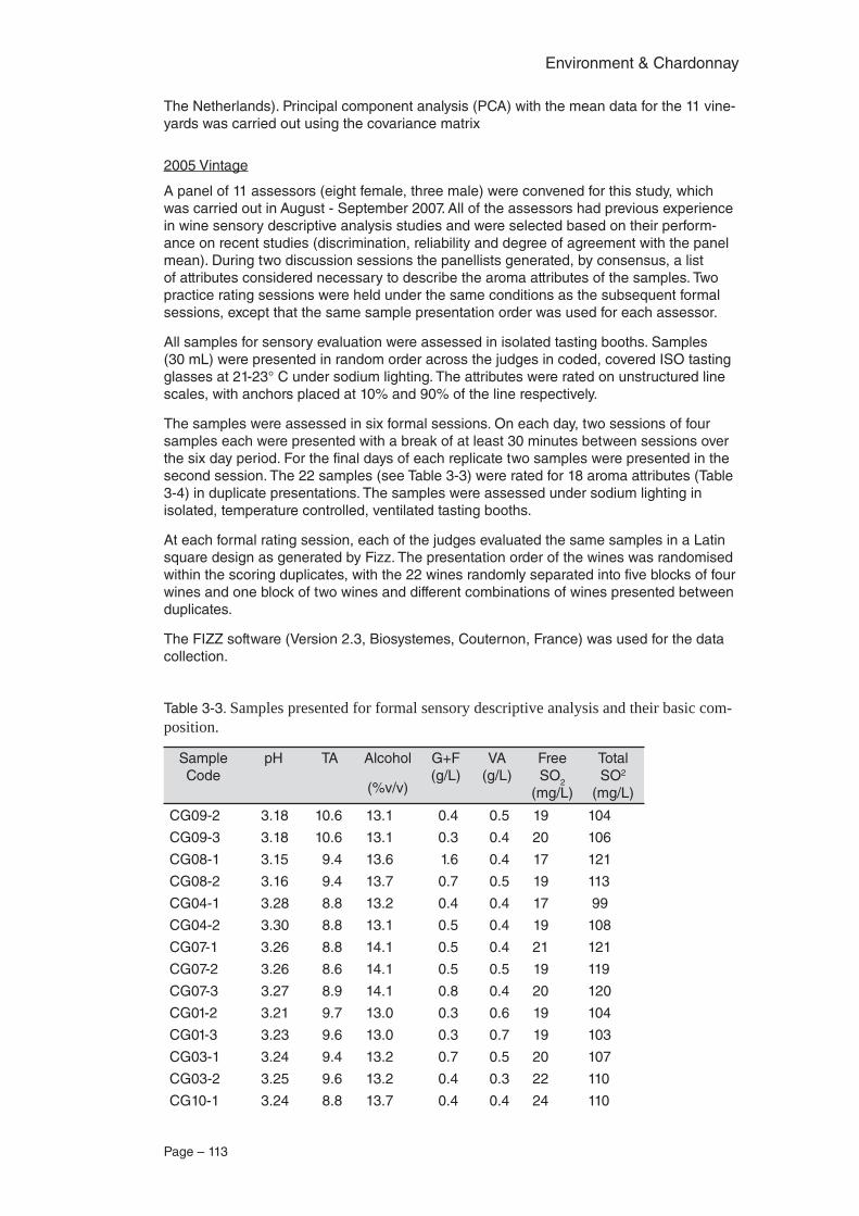
Page – 113
Environment & Chardonnay
The Netherlands). Principal component analysis (PCA) with the mean data for the 11 vine-yards was carried out using the covariance matrix
2005 Vintage
A panel of 11 assessors (eight female, three male) were convened for this study, which was carried out in August - September 2007. All of the assessors had previous experience in wine sensory descriptive analysis studies and were selected based on their perform-ance on recent studies (discrimination, reliability and degree of agreement with the panel mean). During two discussion sessions the panellists generated, by consensus, a list of attributes considered necessary to describe the aroma attributes of the samples. Two practice rating sessions were held under the same conditions as the subsequent formal sessions, except that the same sample presentation order was used for each assessor.
All samples for sensory evaluation were assessed in isolated tasting booths. Samples (30 mL) were presented in random order across the judges in coded, covered ISO tasting glasses at 21-23° C under sodium lighting. The attributes were rated on unstructured line scales, with anchors placed at 10% and 90% of the line respectively.
The samples were assessed in six formal sessions. On each day, two sessions of four samples each were presented with a break of at least 30 minutes between sessions over the six day period. For the final days of each replicate two samples were presented in the second session. The 22 samples (see Table 3-3) were rated for 18 aroma attributes (Table 3-4) in duplicate presentations. The samples were assessed under sodium lighting in isolated, temperature controlled, ventilated tasting booths.
At each formal rating session, each of the judges evaluated the same samples in a Latin square design as generated by Fizz. The presentation order of the wines was randomised within the scoring duplicates, with the 22 wines randomly separated into five blocks of four wines and one block of two wines and different combinations of wines presented between duplicates.
The FIZZ software (Version 2.3, Biosystemes, Couternon, France) was used for the data collection.
Table 3-3. Samples presented for formal sensory descriptive analysis and their basic com-position.
Sample Code
pH TA Alcohol
(%v/v)
G+F (g/L)
VA (g/L)
Free SO2
(mg/L)
Total SO2
(mg/L)
CG09-2 3.18 10.6 13.1 0.4 0.5 19 104
CG09-3 3.18 10.6 13.1 0.3 0.4 20 106
CG08-1 3.15 9.4 13.6 1.6 0.4 17 121
CG08-2 3.16 9.4 13.7 0.7 0.5 19 113
CG04-1 3.28 8.8 13.2 0.4 0.4 17 99
CG04-2 3.30 8.8 13.1 0.5 0.4 19 108
CG07-1 3.26 8.8 14.1 0.5 0.4 21 121
CG07-2 3.26 8.6 14.1 0.5 0.5 19 119
CG07-3 3.27 8.9 14.1 0.8 0.4 20 120
CG01-2 3.21 9.7 13.0 0.3 0.6 19 104
CG01-3 3.23 9.6 13.0 0.3 0.7 19 103
CG03-1 3.24 9.4 13.2 0.7 0.5 20 107
CG03-2 3.25 9.6 13.2 0.4 0.3 22 110
CG10-1 3.24 8.8 13.7 0.4 0.4 24 110
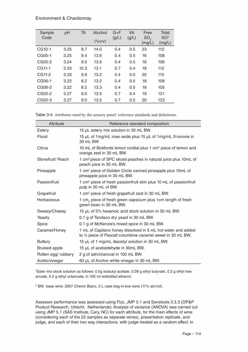
Environment & Chardonnay
Page – 114
Sample Code
pH TA Alcohol
(%v/v)
G+F (g/L)
VA (g/L)
Free SO2
(mg/L)
Total SO2
(mg/L)
CG10-1 3.25 8.7 14.0 0.4 0.5 23 112
CG05-1 3.25 9.4 13.6 0.4 0.5 16 108
CG05-2 3.24 9.0 13.6 0.4 0.5 16 106
CG11-1 3.33 10.3 13.1 0.7 0.4 18 112
CG11-2 3.33 9.9 13.2 0.4 0.5 20 115
CG06-1 3.22 8.2 13.2 0.4 0.5 18 108
CG06-2 3.22 8.2 13.3 0.4 0.5 18 105
CG02-2 3.27 9.0 13.5 0.7 0.4 19 121
CG02-3 3.27 9.0 13.5 0.7 0.5 20 123
Table 3-4. Attributes rated by the sensory panel: reference standards and definitions.
Attribute Reference standard composition
Estery 15 µL estery mix solution in 30 mL BW.
Floral 15 µL of 1mg/mL rose oxide plus 15 µL of 1mg/mL ß-ionone in 30 mL BW.
Citrus 10 mL of Bickfords lemon cordial plus 1 cm2 piece of lemon and orange zest in 30 mL BW.
Stonefruit/ Peach 1 cm2 piece of SPC sliced peaches in natural juice plus 10mL of peach juice in 30 mL BW.
Pineapple 1 cm2 piece of Golden Circle canned pineapple plus 10mL of pineapple juice in 30 mL BW.
Passionfruit 1 cm2 piece of fresh passionfruit skin plus 10 mL of passionfruit pulp in 30 mL of BW.
Grapefruit 1 cm2 piece of fresh grapefruit zest in 30 mL BW.
Herbaceous 1 cm2 piece of fresh green capsicum plus 1cm length of fresh green bean in 30 mL BW.
Sweaty/Cheesy 15 µL of 5% hexanoic acid stock solution in 30 mL BW.
Yeasty 0.1 g of Tandaco dry yeast in 30 mL BW.
Spice 0.1 g of McKenzie’s mixed spice in 30 mL BW.
Caramel/Honey 1 mL of Capilano honey dissolved in 5 mL hot water and added to ¼ piece of Pascall columbine caramel sweet in 30 mL BW.
Buttery 15 µL of 1 mg/mL diacetyl solution in 30 mL BW.
Bruised apple 15 µL of acetaldehyde in 30mL BW.
Rotten egg/ rubbery 2 g of ash/charcoal in 100 mL BW.
Acetic/vinegar 60 µL of Anchor white vinegar in 30 mL BW.
1Ester mix stock solution as follows: 0.5g isobutyl acetate, 0.09 g ethyl butyrate, 0.2 g ethyl hex-anoate, 0.2 g ethyl octanoate, in 100 ml redistilled ethanol.
2 BW base wine: 2007 Chenin Blanc, 2 L cask bag-in-box wine (11% alc/vol).
Assessor performance was assessed using Fizz, JMP 5.1 and Senstools 3.3.3 (OP&P Product Research, Utrecht, Netherlands). Analysis of variance (ANOVA) was carried out using JMP 5.1 (SAS Institute, Cary, NC) for each attribute, for the main effects of wine (considering each of the 22 samples as separate wines), presentation replicate, and judge, and each of their two way interactions, with judge treated as a random effect. In
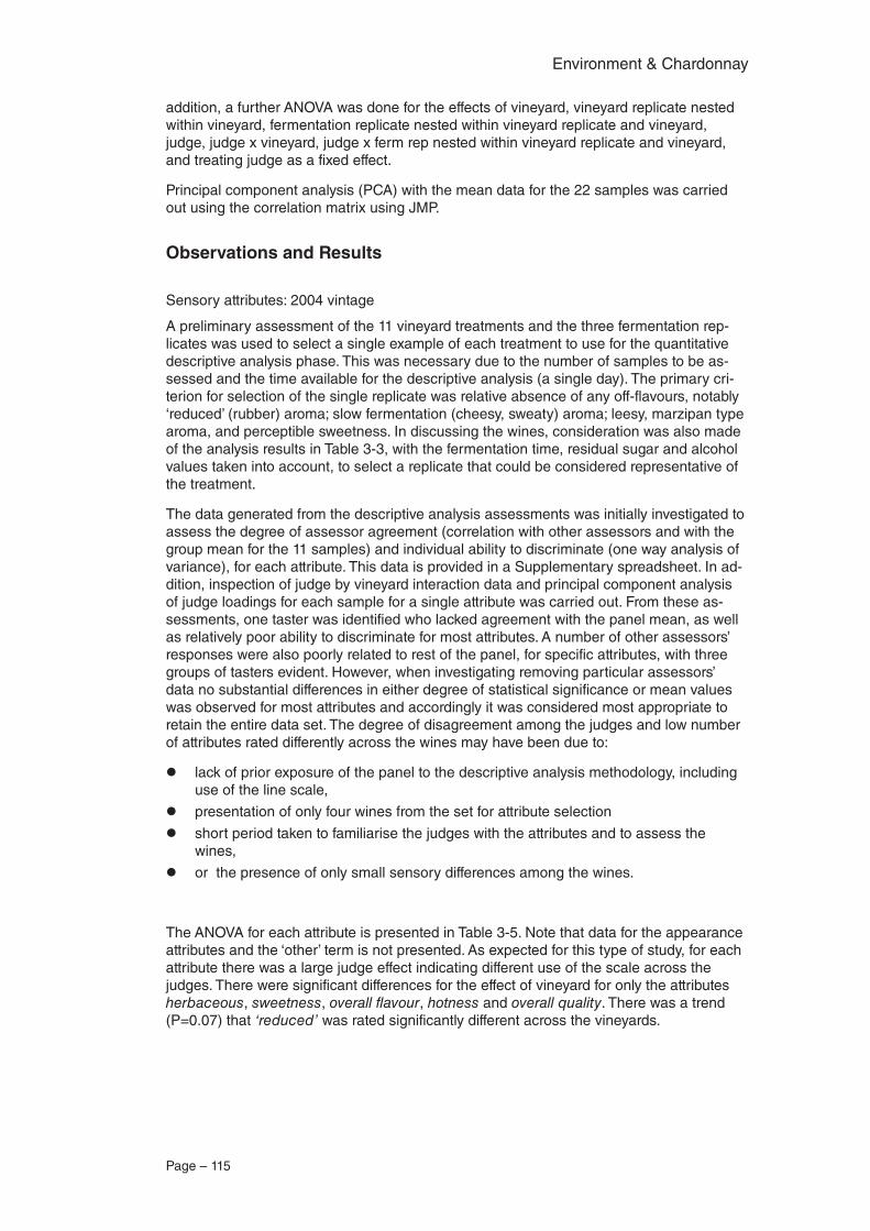
Page – 115
Environment & Chardonnay
addition, a further ANOVA was done for the effects of vineyard, vineyard replicate nested within vineyard, fermentation replicate nested within vineyard replicate and vineyard, judge, judge x vineyard, judge x ferm rep nested within vineyard replicate and vineyard, and treating judge as a fixed effect.
Principal component analysis (PCA) with the mean data for the 22 samples was carried out using the correlation matrix using JMP.
Observations and Results
Sensory attributes: 2004 vintage
A preliminary assessment of the 11 vineyard treatments and the three fermentation rep-licates was used to select a single example of each treatment to use for the quantitative descriptive analysis phase. This was necessary due to the number of samples to be as-sessed and the time available for the descriptive analysis (a single day). The primary cri-terion for selection of the single replicate was relative absence of any off-flavours, notably ‘reduced’ (rubber) aroma; slow fermentation (cheesy, sweaty) aroma; leesy, marzipan type aroma, and perceptible sweetness. In discussing the wines, consideration was also made of the analysis results in Table 3-3, with the fermentation time, residual sugar and alcohol values taken into account, to select a replicate that could be considered representative of the treatment.
The data generated from the descriptive analysis assessments was initially investigated to assess the degree of assessor agreement (correlation with other assessors and with the group mean for the 11 samples) and individual ability to discriminate (one way analysis of variance), for each attribute. This data is provided in a Supplementary spreadsheet. In ad-dition, inspection of judge by vineyard interaction data and principal component analysis of judge loadings for each sample for a single attribute was carried out. From these as-sessments, one taster was identified who lacked agreement with the panel mean, as well as relatively poor ability to discriminate for most attributes. A number of other assessors’ responses were also poorly related to rest of the panel, for specific attributes, with three groups of tasters evident. However, when investigating removing particular assessors’ data no substantial differences in either degree of statistical significance or mean values was observed for most attributes and accordingly it was considered most appropriate to retain the entire data set. The degree of disagreement among the judges and low number of attributes rated differently across the wines may have been due to:
lack of prior exposure of the panel to the descriptive analysis methodology, including use of the line scale,
presentation of only four wines from the set for attribute selection
short period taken to familiarise the judges with the attributes and to assess the wines,
or the presence of only small sensory differences among the wines.
The ANOVA for each attribute is presented in Table 3-5. Note that data for the appearance attributes and the ‘other’ term is not presented. As expected for this type of study, for each attribute there was a large judge effect indicating different use of the scale across the judges. There were significant differences for the effect of vineyard for only the attributes herbaceous, sweetness, overall flavour, hotness and overall quality. There was a trend (P=0.07) that ‘reduced’ was rated significantly different across the vineyards.
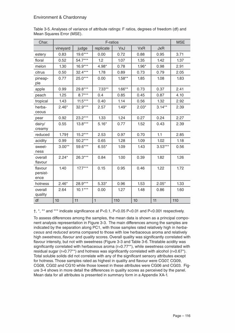
Environment & Chardonnay
Page – 116
Table 3-5. Analyses of variance of attribute ratings: F ratios, degrees of freedom (df) and Mean Squares Error (MSE).
Char. F-ratios MSE
vineyard judge replicate VxJ VxR JxR
estery 0.83 19.6*** 0.00 0.72 0.88 0.95 3.71
floral 0.52 54.7*** 1.2 1.07 1.35 1.42 1.37
melon 1.30 16.9*** 4.98* 0.78 1.96* 0.98 2.91
citrus 0.50 32.4*** 1.78 0.89 0.73 0.79 2.05
pineap-ple
0.77 25.0*** 0.00 1.58** 1.85 1.08 1.83
apple 0.99 29.8*** 7.33** 1.66** 0.73 0.37 2.41
peach 1.25 8.7*** 0.4 0.85 0.45 0.87 4.10
tropical 1.43 11.5*** 0.40 1.14 0.56 1.32 2.92
herba-ceous
2.46* 32.9*** 2.57 1.49* 2.03* 3.14** 2.39
pear 0.92 23.2*** 1.33 1.24 0.27 0.24 2.27
dairy/creamy
0.55 13.8*** 5.16* 0.77 1.52 0.43 2.39
reduced 1.79† 15.2*** 2.53 0.97 0.70 1.1 2.85
acidity 0.99 50.2*** 0.65 1.28 1.09 1.02 1.18
sweet-ness
3.00** 59.6*** 6.55* 1.09 1.43 3.53*** 0.56
overall flavour
2.24* 26.3*** 0.84 1.00 0.39 1.82 1.26
flavour persist-ence
1.40 17.7*** 0.15 0.95 0.46 1.22 1.72
hotness 2.46* 28.9*** 5.33* 0.96 1.53 2.05* 1.33
overall quality
2.64 10.1*** 0.00 1.27 1.48 0.86 1.60
df 10 11 1 110 10 11 110
†, *, ** and *** indicate significance at P<0.1, P<0.05 P<0.01 and P<0.001 respectively.
To assess differences among the samples, the mean data is shown as a principal compo-nent analysis representation in Figure 3-3. The main differences among the samples are indicated by the separation along PC1, with those samples rated relatively high in herba-ceous and reduced aroma compared to those with low herbaceous aroma and relatively high sweetness, flavour and quality scores. Overall quality was significantly correlated with flavour intensity, but not with sweetness (Figure 3-3 and Table 3-6. Titratable acidity was significantly correlated with herbaceous aroma (r=0.77**), while sweetness correlated with residual sugar (r=0.77**) and hotness was significantly correlated with alcohol (r=0.67*). Total soluble solids did not correlate with any of the significant sensory attributes except for hotness. Those samples rated as highest in quality and flavour were CG07, CG09, CG08, CG02 and CG10 while those lowest in these attributes were CG06 and CG03. Fig-ure 3-4 shows in more detail the differences in quality scores as perceived by the panel. Mean data for all attributes is presented in summary form in a Appendix XA-1.
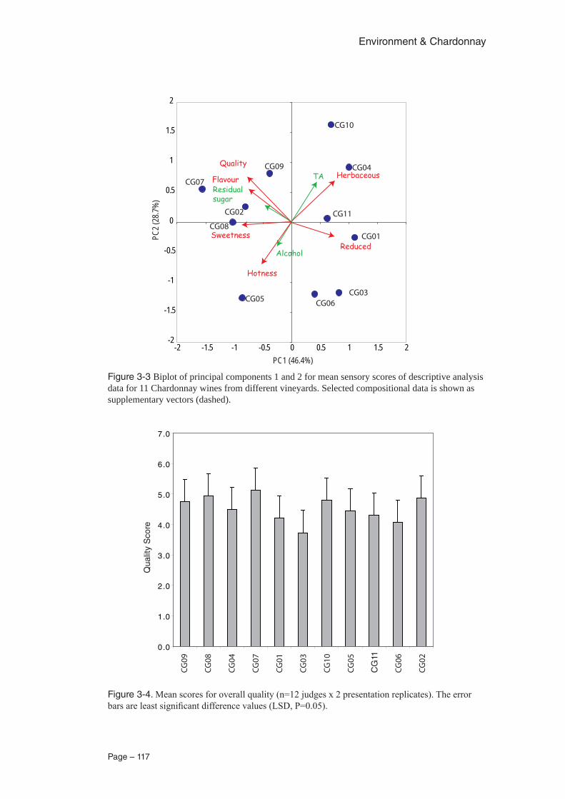
Page – 117
Environment & Chardonnay
Figure 3-3 Biplot of principal components 1 and 2 for mean sensory scores of descriptive analysis data for 11 Chardonnay wines from different vineyards. Selected compositional data is shown as supplementary vectors (dashed).
Figure 3-4. Mean scores for overall quality (n=12 judges x 2 presentation replicates). The error bars are least significant difference values (LSD, P=0.05).
-2
-1.5
-1
-0.5
0
0.5
1
1.5
2
-2 -1.5 -1 -0.5 0 0.5 1 1.5 2
CG10
CG04
CG11
CG01
CG03CG06CG05
CG08
CG02
CG07
CG09Herbaceous
Quality
FlavourResidualsugar
SweetnessReduced
Alcohol
Hotness
TA
PC2 (
28.7%
)
PC1 (46.4%)
0.0
1.0
2.0
3.0
4.0
5.0
6.0
7.0
CG
01
CG
02
CG
03
CG
04
CG
05
CG
06
CG
07
CG
08
CG
09
CG
10
CG
11
Qua
lity
Sco
re
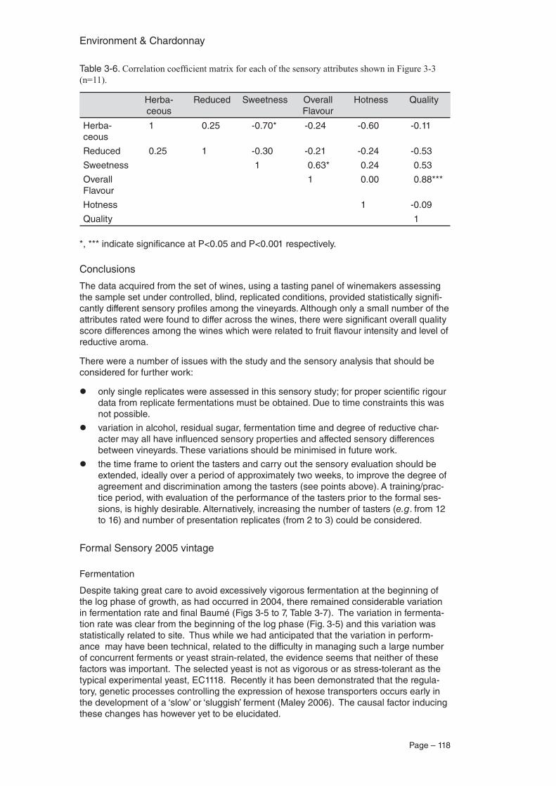
Environment & Chardonnay
Page – 118
Table 3-6. Correlation coefficient matrix for each of the sensory attributes shown in Figure 3-3 (n=11).
Herba-ceous
Reduced Sweetness Overall Flavour
Hotness Quality
Herba-ceous
1 0.25 -0.70* -0.24 -0.60 -0.11
Reduced 0.25 1 -0.30 -0.21 -0.24 -0.53
Sweetness 1 0.63* 0.24 0.53
Overall Flavour
1 0.00 0.88***
Hotness 1 -0.09
Quality 1
*, *** indicate significance at P<0.05 and P<0.001 respectively.
Conclusions
The data acquired from the set of wines, using a tasting panel of winemakers assessing the sample set under controlled, blind, replicated conditions, provided statistically signifi-cantly different sensory profiles among the vineyards. Although only a small number of the attributes rated were found to differ across the wines, there were significant overall quality score differences among the wines which were related to fruit flavour intensity and level of reductive aroma.
There were a number of issues with the study and the sensory analysis that should be considered for further work:
only single replicates were assessed in this sensory study; for proper scientific rigour data from replicate fermentations must be obtained. Due to time constraints this was not possible.
variation in alcohol, residual sugar, fermentation time and degree of reductive char-acter may all have influenced sensory properties and affected sensory differences between vineyards. These variations should be minimised in future work.
the time frame to orient the tasters and carry out the sensory evaluation should be extended, ideally over a period of approximately two weeks, to improve the degree of agreement and discrimination among the tasters (see points above). A training/prac-tice period, with evaluation of the performance of the tasters prior to the formal ses-sions, is highly desirable. Alternatively, increasing the number of tasters (e.g. from 12 to 16) and number of presentation replicates (from 2 to 3) could be considered.
Formal Sensory 2005 vintage
Fermentation
Despite taking great care to avoid excessively vigorous fermentation at the beginning of the log phase of growth, as had occurred in 2004, there remained considerable variation in fermentation rate and final Baumé (Figs 3-5 to 7, Table 3-7). The variation in fermenta-tion rate was clear from the beginning of the log phase (Fig. 3-5) and this variation was statistically related to site. Thus while we had anticipated that the variation in perform-ance may have been technical, related to the difficulty in managing such a large number of concurrent ferments or yeast strain-related, the evidence seems that neither of these factors was important. The selected yeast is not as vigorous or as stress-tolerant as the typical experimental yeast, EC1118. Recently it has been demonstrated that the regula-tory, genetic processes controlling the expression of hexose transporters occurs early in the development of a ‘slow’ or ‘sluggish’ ferment (Maley 2006). The causal factor inducing these changes has however yet to be elucidated.
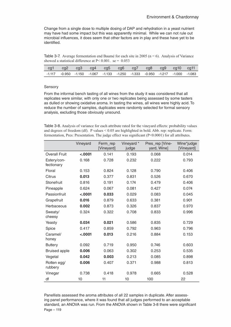
Page – 119
Environment & Chardonnay
Change from a single dose to multiple dosing of DAP and rehydration in a yeast nutrient may have had some impact but this was apparently minimal. While we can not rule out microbial influences, it does seem that other factors are in play and these have yet to be identified.
Table 3-7. Average fermentation end Baumé for each site in 2005 (n = 6). Analysis of Variance showed a statistical difference at P< 0.001. se = 0.053
cg1 cg2 cg3 cg4 cg5 cg6 cg7 cg8 cg9 cg10 cg11
-1.117 -0.950 -1.150 -1.067 -1.133 -1.250 -1.333 -0.950 -1.217 -1.000 -1.083
Sensory
From the informal bench tasting of all wines from the study it was considered that all replicates were similar, with only one or two replicates being assessed by some tasters as dulled or showing oxidative aroma. In tasting the wines, all wines were highly acid. To reduce the number of samples, duplicates were randomly selected for formal sensory analysis, excluding those obviously unsound.
Table 3-8. Analysis of variance for each attribute rated for the vineyard effects: probability values and degrees of freedom (df). P values < 0.05 are highlighted in bold. Abb. rep: replicate. Ferm: fermentation, Pres: Presentation. The judge effect was significant (P<0.0001) for all attributes.
Vineyard Ferm_rep [Vineyard]
Vineyard * judge
Pres_rep [Vine-yard, Wine]
Wine*judge [Vineyard]
Overall Fruit <.0001 0.141 0.193 0.068 0.014
Estery/con-fectionary
0.168 0.728 0.232 0.222 0.793
Floral 0.153 0.824 0.128 0.790 0.406
Citrus 0.013 0.377 0.831 0.526 0.670
Stonefruit 0.816 0.191 0.174 0.479 0.406
Pineapple 0.624 0.067 0.081 0.427 0.074
Passionfruit <.0001 0.033 0.029 0.083 0.045
Grapefruit 0.016 0.879 0.633 0.381 0.901
Herbaceous 0.002 0.873 0.326 0.837 0.970
Sweaty/cheesy
0.324 0.322 0.708 0.833 0.996
Yeasty 0.034 0.021 0.586 0.835 0.729
Spice 0.417 0.859 0.792 0.963 0.796
Caramel/ honey
<.0001 0.013 0.216 0.884 0.153
Buttery 0.092 0.719 0.950 0.746 0.603
Bruised apple 0.006 0.063 0.302 0.253 0.535
Vegetal 0.042 0.003 0.213 0.085 0.898
Rotten egg/ rubbery
0.006 0.407 0.371 0.988 0.813
Vinegar 0.738 0.418 0.978 0.665 0.528
df 10 11 10 100 22
Panellists assessed the aroma attributes of all 22 samples in duplicate. After assess-ing panel performance, where it was found that all judges performed to an acceptable standard, an ANOVA was run. From the ANOVA shown in Table 3-8 there were significant
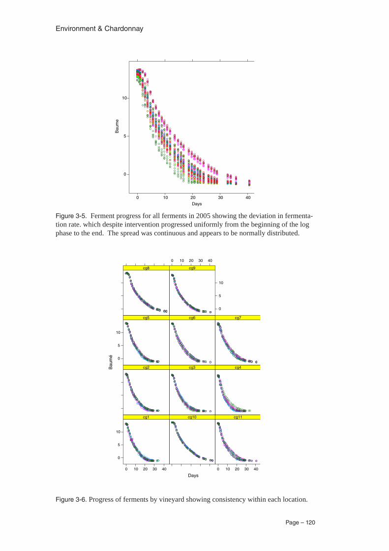
Environment & Chardonnay
Page – 120
C
M
Y
CM
MY
CY
CMY
K
wine.ferm05.pdf 15/04/09 10:58:49 PM
C
M
Y
CM
MY
CY
CMY
K
wine.ferm05.vd.pdf 15/04/09 11:02:49 PM
Figure 3-5. Ferment progress for all ferments in 2005 showing the deviation in fermenta-tion rate. which despite intervention progressed uniformly from the beginning of the log phase to the end. The spread was continuous and appears to be normally distributed.
Figure 3-6. Progress of ferments by vineyard showing consistency within each location.
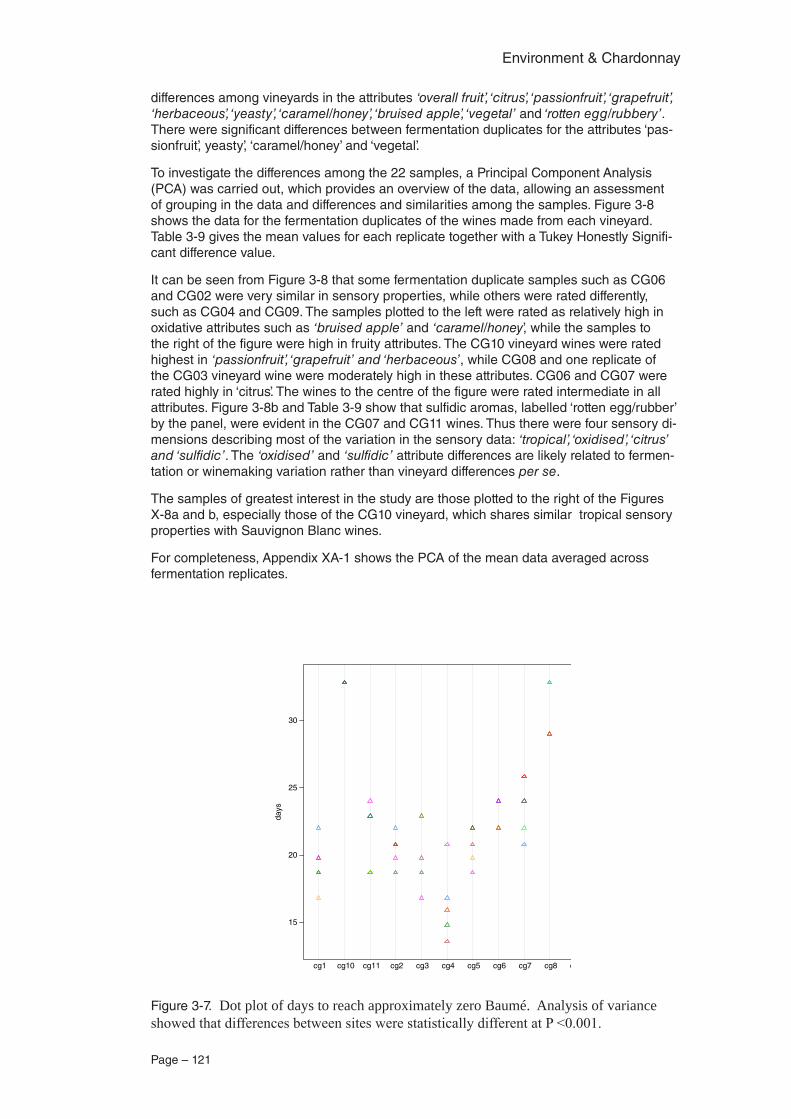
Page – 121
Environment & Chardonnay
differences among vineyards in the attributes ‘overall fruit’, ‘citrus’, ‘passionfruit’, ‘grapefruit’, ‘herbaceous’, ‘yeasty’, ‘caramel/honey’, ‘bruised apple’, ‘vegetal’ and ‘rotten egg/rubbery’. There were significant differences between fermentation duplicates for the attributes ‘pas-sionfruit’, yeasty’, ‘caramel/honey’ and ‘vegetal’.
To investigate the differences among the 22 samples, a Principal Component Analysis (PCA) was carried out, which provides an overview of the data, allowing an assessment of grouping in the data and differences and similarities among the samples. Figure 3-8 shows the data for the fermentation duplicates of the wines made from each vineyard. Table 3-9 gives the mean values for each replicate together with a Tukey Honestly Signifi-cant difference value.
It can be seen from Figure 3-8 that some fermentation duplicate samples such as CG06 and CG02 were very similar in sensory properties, while others were rated differently, such as CG04 and CG09. The samples plotted to the left were rated as relatively high in oxidative attributes such as ‘bruised apple’ and ‘caramel/honey’, while the samples to the right of the figure were high in fruity attributes. The CG10 vineyard wines were rated highest in ‘passionfruit’, ‘grapefruit’ and ‘herbaceous’, while CG08 and one replicate of the CG03 vineyard wine were moderately high in these attributes. CG06 and CG07 were rated highly in ‘citrus’. The wines to the centre of the figure were rated intermediate in all attributes. Figure 3-8b and Table 3-9 show that sulfidic aromas, labelled ‘rotten egg/rubber’ by the panel, were evident in the CG07 and CG11 wines. Thus there were four sensory di-mensions describing most of the variation in the sensory data: ‘tropical’, ‘oxidised’, ‘citrus’ and ‘sulfidic’. The ‘oxidised’ and ‘sulfidic’ attribute differences are likely related to fermen-tation or winemaking variation rather than vineyard differences per se.
The samples of greatest interest in the study are those plotted to the right of the Figures X-8a and b, especially those of the CG10 vineyard, which shares similar tropical sensory properties with Sauvignon Blanc wines.
For completeness, Appendix XA-1 shows the PCA of the mean data averaged across fermentation replicates.
C
M
Y
CM
MY
CY
CMY
K
ferm.end.05.pdf 15/04/09 9:12:58 PM
Figure 3-7. Dot plot of days to reach approximately zero Baumé. Analysis of variance showed that differences between sites were statistically different at P <0.001.
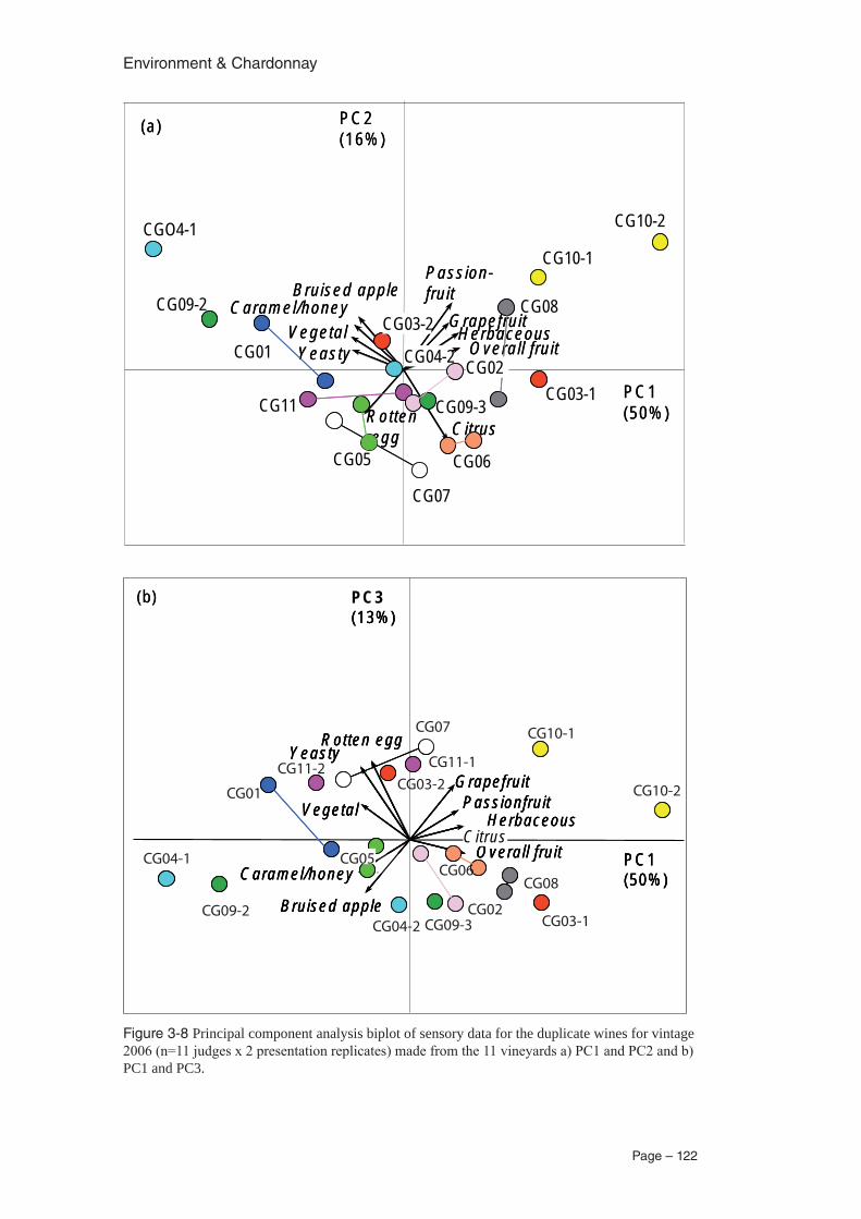
Environment & Chardonnay
Page – 122
CG09-2
CG09-3
CG08
CGO4-1
CG07
CG01
CG03-1
CG10-1
CG10-2
CG05
CG11
CG06
O vera ll fru it
C itrus
P ass ion-fru it
G rapefru itH erbaceous
Y easty
C aram el/honeyB ru ised app le
V egeta l
R ottenegg
B R O 2 W O D
G E O 2
P C 1 (50% )
P C 2(16% )
(a)
O vera ll fru it
C itrus
P ass ion-fru it
G rapefru itH erbaceous
Y easty
C aram el/honeyB ru ised app le
V egeta l
R ottenegg
CG04-2 CG02
CG03-2
P C 1 (50% )
P C 2(16% )
(a)
O vera ll fru it
P ass ionfru itG rapefru it
H erbaceous
Y easty
C aram el/honey
B ru ised app le
V egeta l
R otten egg
C itrusP C 1 (50% )
PC3(13% )
JIN
(b)
O vera ll fru it
P ass ionfru itG rapefru it
H erbaceous
Y easty
C aram el/honey
B ru ised app le
V egeta l
R otten egg
C itrusP C 1 (50% )
(13% )
O vera ll fru it
P ass ionfru itG rapefru it
H erbaceous
Y easty
C aram el/honey
B ru ised app le
V egeta l
R otten egg
C itrusP C 1 (50% )
(13% )(b)
CG10-1
CG10-2
CG07
CG11-1CG11-2
CG01CG03-2
CG03-1
CG08
CG02CG09-3
CG09-2
CG04-1
CG04-2
CG06CG05
Figure 3-8 Principal component analysis biplot of sensory data for the duplicate wines for vintage 2006 (n=11 judges x 2 presentation replicates) made from the 11 vineyards a) PC1 and PC2 and b) PC1 and PC3.
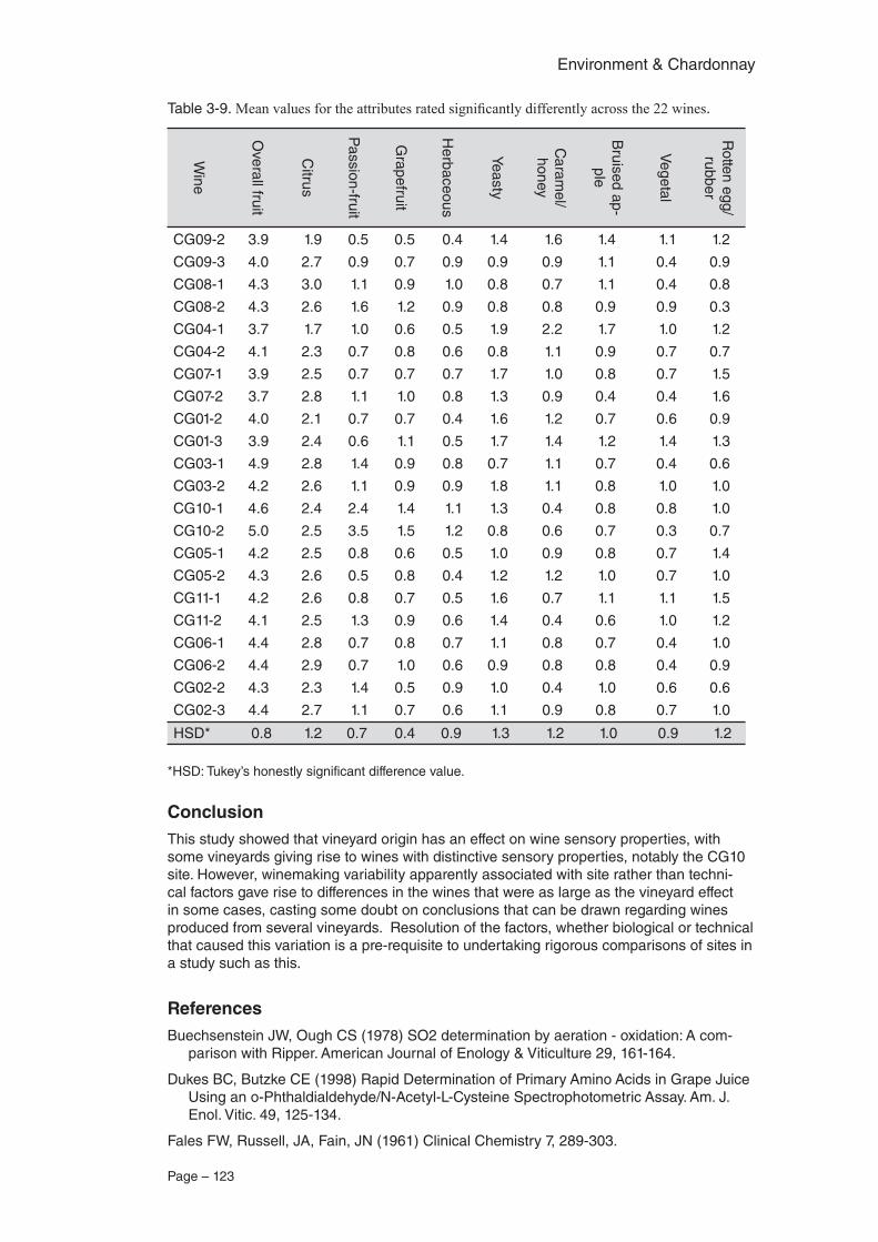
Page – 123
Environment & Chardonnay
Table 3-9. Mean values for the attributes rated significantly differently across the 22 wines.
Wine
Overall fruit
Citrus
Passion-fruit
Grapefruit
Herbaceous
Yeasty
Caram
el/ honey
Bruised ap-
ple
Vegetal
Rotten egg/ rubber
CG09-2 3.9 1.9 0.5 0.5 0.4 1.4 1.6 1.4 1.1 1.2
CG09-3 4.0 2.7 0.9 0.7 0.9 0.9 0.9 1.1 0.4 0.9
CG08-1 4.3 3.0 1.1 0.9 1.0 0.8 0.7 1.1 0.4 0.8
CG08-2 4.3 2.6 1.6 1.2 0.9 0.8 0.8 0.9 0.9 0.3
CG04-1 3.7 1.7 1.0 0.6 0.5 1.9 2.2 1.7 1.0 1.2
CG04-2 4.1 2.3 0.7 0.8 0.6 0.8 1.1 0.9 0.7 0.7
CG07-1 3.9 2.5 0.7 0.7 0.7 1.7 1.0 0.8 0.7 1.5
CG07-2 3.7 2.8 1.1 1.0 0.8 1.3 0.9 0.4 0.4 1.6
CG01-2 4.0 2.1 0.7 0.7 0.4 1.6 1.2 0.7 0.6 0.9
CG01-3 3.9 2.4 0.6 1.1 0.5 1.7 1.4 1.2 1.4 1.3
CG03-1 4.9 2.8 1.4 0.9 0.8 0.7 1.1 0.7 0.4 0.6
CG03-2 4.2 2.6 1.1 0.9 0.9 1.8 1.1 0.8 1.0 1.0
CG10-1 4.6 2.4 2.4 1.4 1.1 1.3 0.4 0.8 0.8 1.0
CG10-2 5.0 2.5 3.5 1.5 1.2 0.8 0.6 0.7 0.3 0.7
CG05-1 4.2 2.5 0.8 0.6 0.5 1.0 0.9 0.8 0.7 1.4
CG05-2 4.3 2.6 0.5 0.8 0.4 1.2 1.2 1.0 0.7 1.0
CG11-1 4.2 2.6 0.8 0.7 0.5 1.6 0.7 1.1 1.1 1.5
CG11-2 4.1 2.5 1.3 0.9 0.6 1.4 0.4 0.6 1.0 1.2
CG06-1 4.4 2.8 0.7 0.8 0.7 1.1 0.8 0.7 0.4 1.0
CG06-2 4.4 2.9 0.7 1.0 0.6 0.9 0.8 0.8 0.4 0.9
CG02-2 4.3 2.3 1.4 0.5 0.9 1.0 0.4 1.0 0.6 0.6
CG02-3 4.4 2.7 1.1 0.7 0.6 1.1 0.9 0.8 0.7 1.0
HSD* 0.8 1.2 0.7 0.4 0.9 1.3 1.2 1.0 0.9 1.2
*HSD: Tukey’s honestly significant difference value.
ConclusionThis study showed that vineyard origin has an effect on wine sensory properties, with some vineyards giving rise to wines with distinctive sensory properties, notably the CG10 site. However, winemaking variability apparently associated with site rather than techni-cal factors gave rise to differences in the wines that were as large as the vineyard effect in some cases, casting some doubt on conclusions that can be drawn regarding wines produced from several vineyards. Resolution of the factors, whether biological or technical that caused this variation is a pre-requisite to undertaking rigorous comparisons of sites in a study such as this.
ReferencesBuechsenstein JW, Ough CS (1978) SO2 determination by aeration - oxidation: A com-
parison with Ripper. American Journal of Enology & Viticulture 29, 161-164.
Dukes BC, Butzke CE (1998) Rapid Determination of Primary Amino Acids in Grape Juice Using an o-Phthaldialdehyde/N-Acetyl-L-Cysteine Spectrophotometric Assay. Am. J. Enol. Vitic. 49, 125-134.
Fales FW, Russell, JA, Fain, JN (1961) Clinical Chemistry 7, 289-303.
Environment & Chardonnay
Page – 124
Gladstones, J. S. (1992). Viticulture and Environment. Adelaide, Winetitles.
Jones GV, Davis RE (2000) Climate influences on grapevine phenology, grape composi-tion, and wine production and quality for Bordeaux, France. American Journal of Enol-ogy and Viticulture 51, 249-261.
Lawless, H.T., and H. Heymann. (1998) Sensory Evaluation of Food: Principles and Prac-tices. New York: Chapman and Hall.
Maley, K. (2006) Hexose transporter gene expression during stuck and sluggish wine fer-mentations. Perth: Honours thesis, School of Biomedical, Biomolecular and Chemical Sciences, University of Western Australia.
Rankine BC (1970) Alkalimetric determination of sulphur dioxide in wine. Australian Wine, Brewing and Spirit Review 88, 40-44.
Somogyi, M (1952) Journal of Biological Chemistry 195, 19-23.
White, R. E. (2003). Soils for Fine Wines. NY, Oxford University Press.
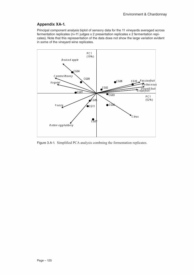
Page – 125
Environment & Chardonnay
CG09CG08
CG04
CG07
CG01CG03
CG10
CG05
CG11 CG06
CG02 O vera ll fru it
C itrus
P ass ion fru it
G rapefru it
H erbaceous
Yeasty
C aram el/honey
B ru ised app le
V egeta l
R o tten egg /rubbery
PC1(52% )
PC1(19% )
Figure 3.A-1. Simplified PCA analysis combning the fermentation replicates.
Appendix XA-1. Principal component analysis biplot of sensory data for the 11 vineyards averaged across fermentation replicates (n=11 judges x 2 presentation replicates x 2 fermentation repi-cates). Note that this representation of the data does not show the large variation evident in some of the vineyard wine replicates.

Environment & Chardonnay
Page – 126
Page – 127
Environment & Chardonnay
The Vineyards and Their Characteristics
Author: J.A. Considine, School of Plant Biology, The University of Western Australia, Crawley 6009
Abstract
Vineyards under showed evidence of sub-optimal flower initiation and retention leading to lower yields and higher vegetative indexes. This was supported by the lack of a correlation between bud retention and pruning weights. Some vineyards showed budburst values that were well in excess of the bud number retained at pruning suggesting changes to canopy management practice may be beneficial. There was also strong evidence of a lack of adap-tive pruning practices within vineyards again leading to sub-optimal performance. As no vineyard in the study was fully mechanically pruned, there is an opportunity to improve labour training to optimise vine performance within a vineyard and from year to year.
IntroductionThis project sets out to examine the relationship between site and wine quality for the cultivar “Gingin” cv, Chardonnay. This section describes the productivity of the vineyards for three successive season to provide an essential background to interpretation of wine sensory qualities. Other aspects of each vineyard are described in the remote sensing sections of this report.
Materials and MethodsThese are described in Appendix 1: Operating Procedures.
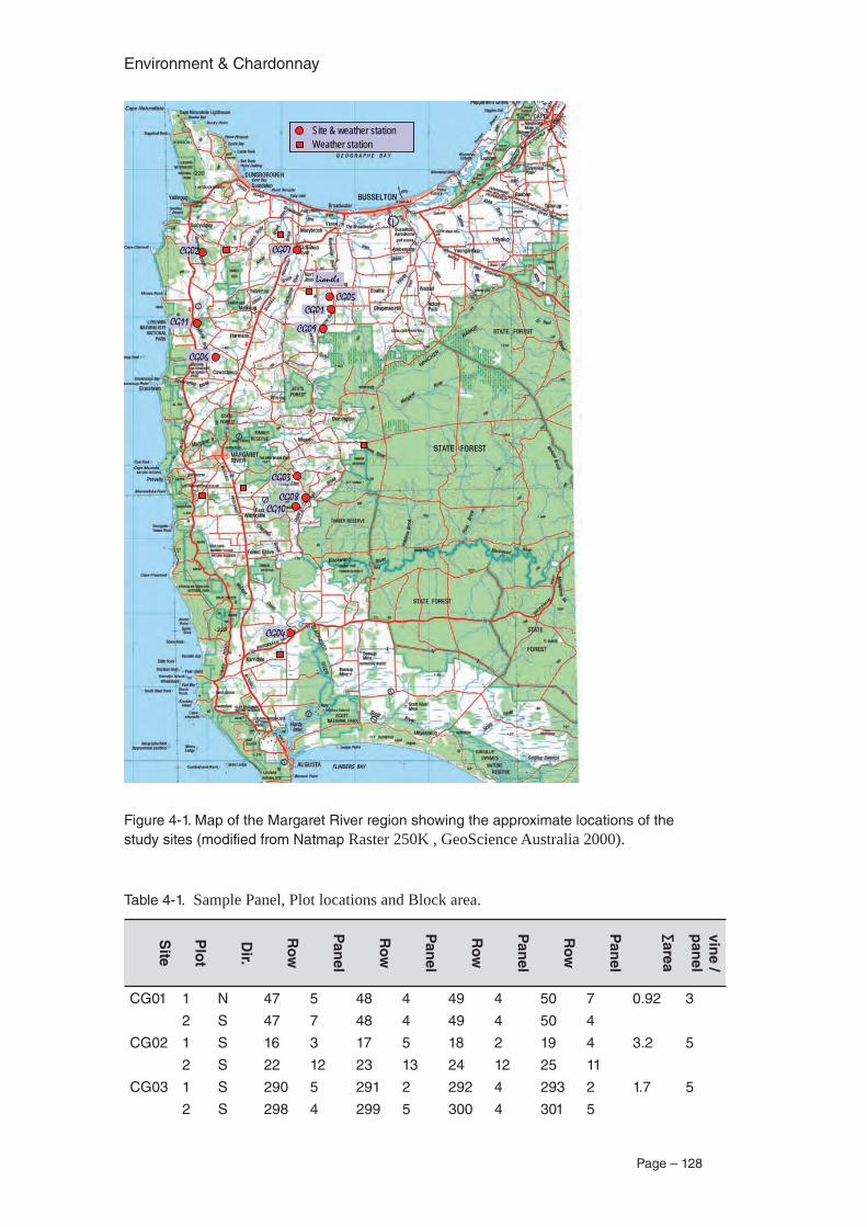
Environment & Chardonnay
Page – 128
7
Site & weather station
Lionels
CG10CG08
CG03
CG04
CG06
CG11CG09
CG01CG05
CG02 CG07
Weather station
Figure 4-1. Map of the Margaret River region showing the approximate locations of the study sites (modified from Natmap Raster 250K , GeoScience Australia 2000).
Table 4-1. Sample Panel, Plot locations and Block area.
Site
Plo
t
Dir.
Ro
w
Pan
el
Ro
w
Pan
el
Ro
w
Pan
el
Ro
w
Pan
el
∑area
vine /
pan
el
CG01 1 N 47 5 48 4 49 4 50 7 0.92 3
2 S 47 7 48 4 49 4 50 4
CG02 1 S 16 3 17 5 18 2 19 4 3.2 5
2 S 22 12 23 13 24 12 25 11
CG03 1 S 290 5 291 2 292 4 293 2 1.7 5
2 S 298 4 299 5 300 4 301 5
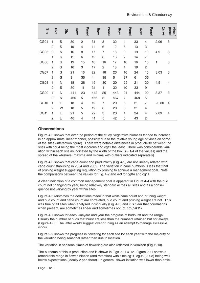
Page – 129
Environment & Chardonnay
Site
Plo
t
Dir.
Ro
w
Pan
el
Ro
w
Pan
el
Ro
w
Pan
el
Ro
w
Pan
el
∑area
vine /
pan
el
CG04 1 S 30 2 31 3 32 4 33 4 2.06 3
2 S 10 4 11 6 12 5 13 3
CG05 2 N 16 8 17 7 18 9 19 10 4.9 3
1 S 11 6 12 8 13 7 14 7
CG06 1 S 19 15 18 16 17 16 16 15 1 6
2 S 16 3 17 2 18 4 19 2
CG07 1 S 21 16 22 16 23 16 24 15 3.03 3
2 S 3 35 4 35 5 37 6 36
CG08 1 N 18 28 19 30 20 29 21 30 4.5 4
2 S 30 11 31 11 32 10 33 9
CG09 1 N 441 23 442 25 443 24 444 22 3.37 3
2 N 465 5 466 5 467 7 468 5
CG10 1 E 18 4 19 7 20 6 21 7 ~0.80 4
2 W 18 5 19 6 20 6 21 4
CG11 1 E 21 5 22 3 23 4 24 4 2.09 4
2 E 40 4 41 5 42 5 43 2
ObservationsFigure 4-2 shows that over the period of the study, vegetative biomass tended to increase in an approximate linear manner, possibly due to the relative young age of vines on some of the sites (interaction figure). There were notable differences in productivity between the sites with cg04 being the most vigorous and cg11 the least. There was considerable vari-ation within each site as indicated by the width of the box (+\- 1/4 of the values) and the spread of the whiskers (maxima and minima with outliers indicated separately).
Figure 4-3 shows that cane count and productivity (Fig. 4-2) are not linearly related with cane count stabilising in 2004 and 2005. The variation in cane numbers is less that that of pruning weight suggesting regulation by pruning to achieve a managment goal. Note the comparisons between the values for Fig. 4-2 and 4-3 for cg04 and cg11.
A clear indication of a common management goal is apparent in Figure 4-4 with the bud count not changing by year, being relatively standard across all sites and as a conse-quence not varying by year within sites.
Figure 4-5 reinforces the deductions made in that while cane count and pruning weight and bud count and cane count are correlated, bud count and pruning weight are not. This was true of all sites when analysed individually (Fig. 4-6) and it is clear that correlations when present, are sometimes linear and sometimes not (cf. cg2,5&11).
Figure 4-7 shows for each vineyard and year the progress of budburst and the range. Usually the number of buds that burst are less than the numbers retained but not always (Figure 4-8). The latter would suggest over-pruning as an attempt to manage excessive vigour.
Figure 2-9 shows the progress in flowering for each site for each year with the majority of the variation being seasonal rather than due to location.
The variation in seasonal times of flowering are also reflected in veraison (Fig. 2-10).
The outcome of this is production and is shown in Figs 2-11 & 12. Figure 2-11 shows a remarkable range in flower iniation (and retention) with sites cg11, cg06 (2003) being well below expectations (ideally 2 per shoot). In general, flower initiation was lower than antici-

Environment & Chardonnay
Page – 130
pated for a warm region though cloud cover can be high during the flower initiation period. However, the data suggests that other factors may be involved.
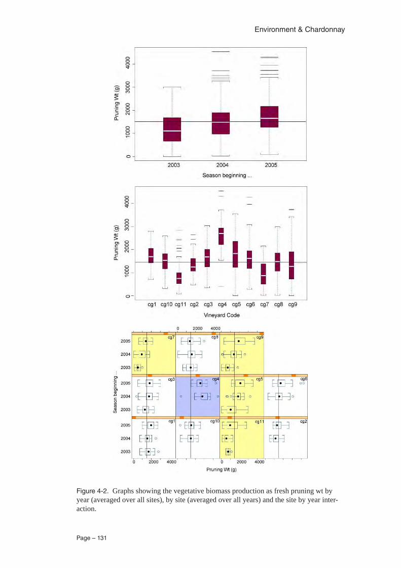
Page – 131
Environment & Chardonnay
Figure 4-2. Graphs showing the vegetative biomass production as fresh pruning wt by year (averaged over all sites), by site (averaged over all years) and the site by year inter-action.
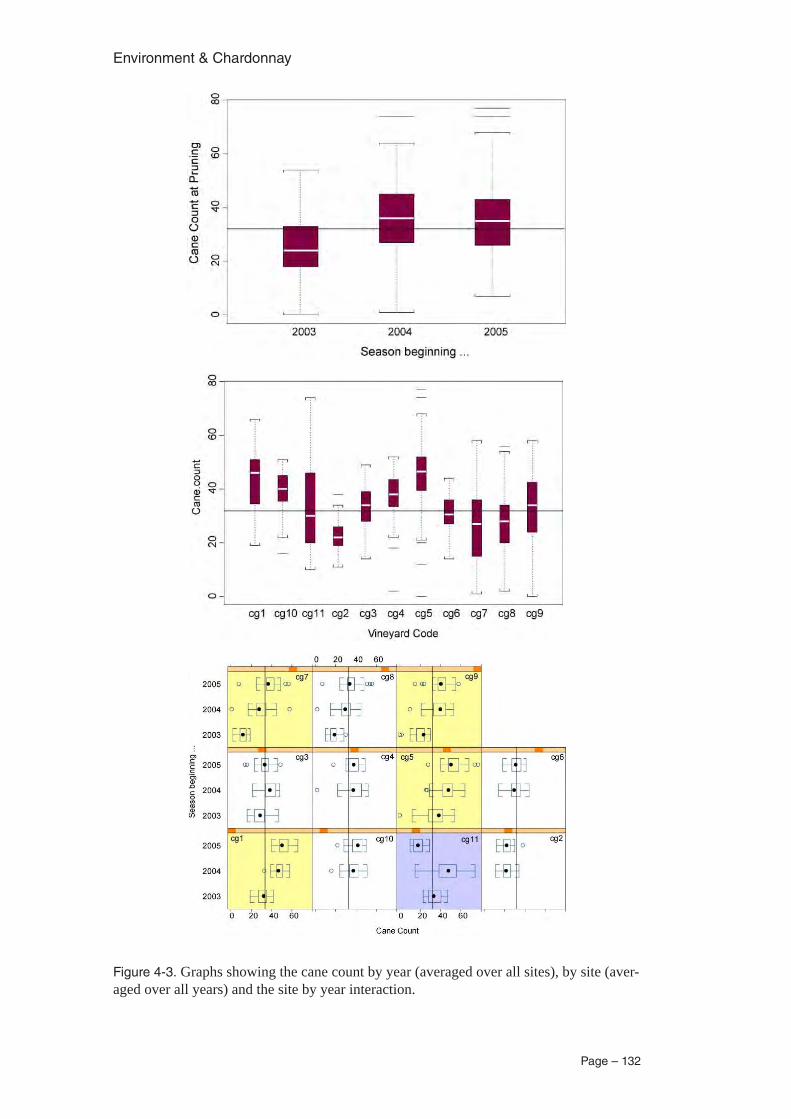
Environment & Chardonnay
Page – 132
Figure 4-3. Graphs showing the cane count by year (averaged over all sites), by site (aver-aged over all years) and the site by year interaction.
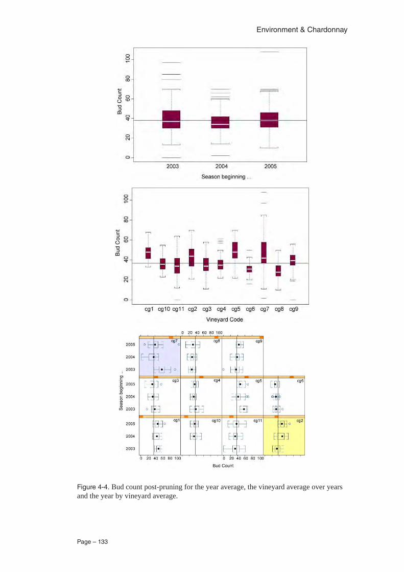
Page – 133
Environment & Chardonnay
Figure 4-4. Bud count post-pruning for the year average, the vineyard average over years and the year by vineyard average.
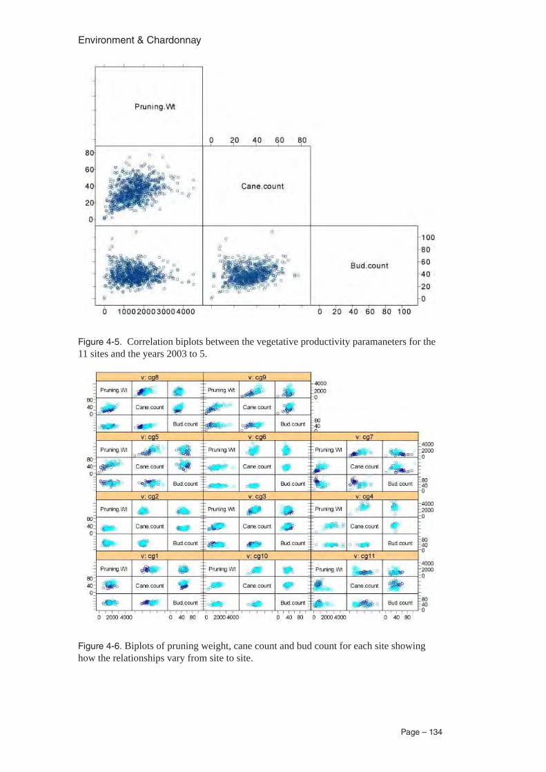
Environment & Chardonnay
Page – 134
Figure 4-5. Correlation biplots between the vegetative productivity paramaneters for the 11 sites and the years 2003 to 5.
Figure 4-6. Biplots of pruning weight, cane count and bud count for each site showing how the relationships vary from site to site.
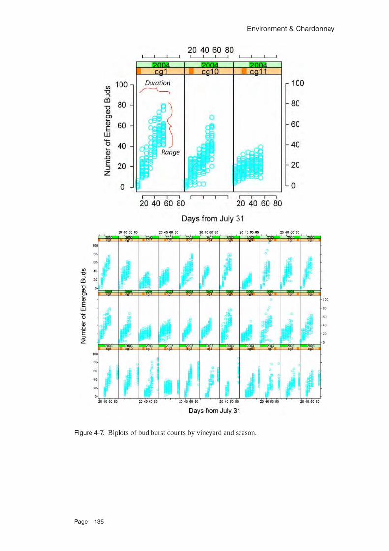
Page – 135
Environment & Chardonnay
Figure 4-7. Biplots of bud burst counts by vineyard and season.
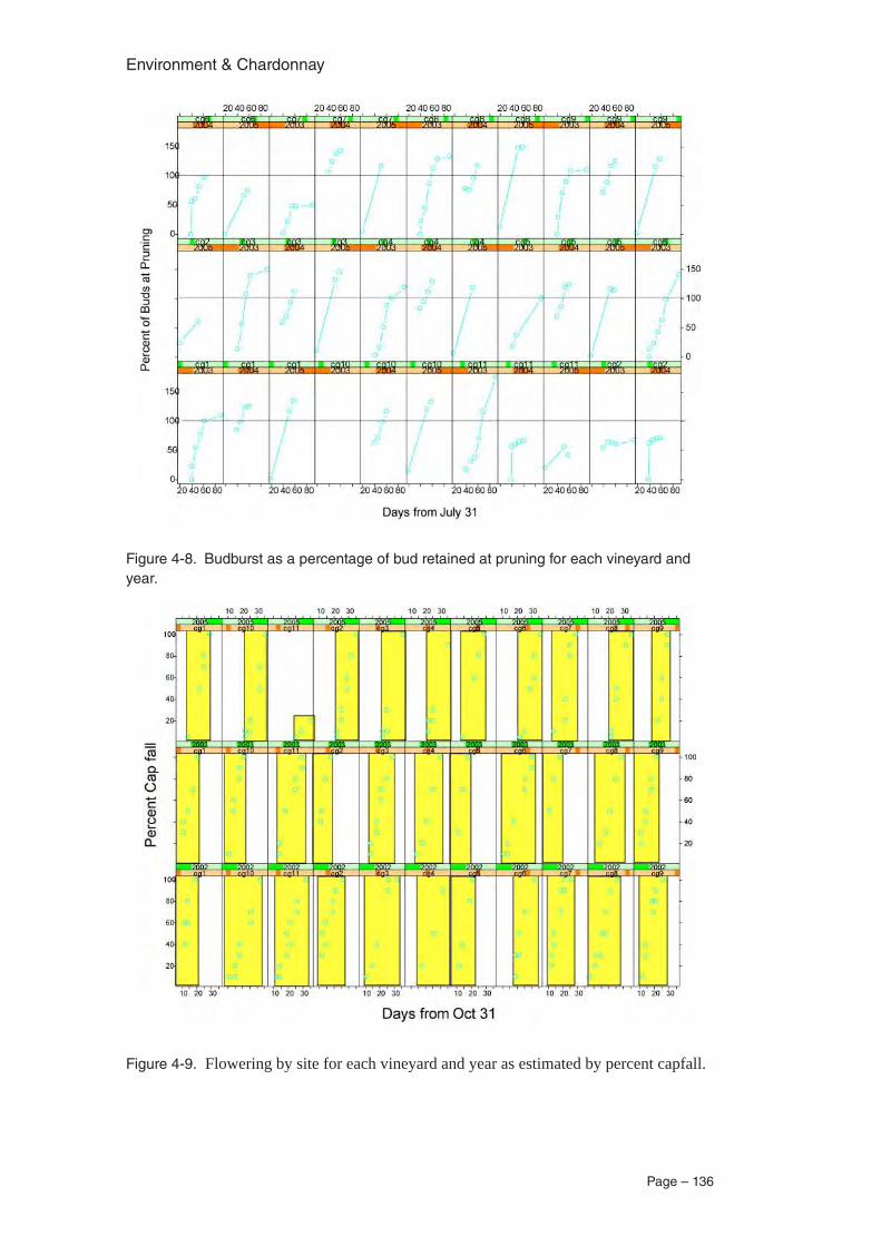
Environment & Chardonnay
Page – 136
Figure 4-8. Budburst as a percentage of bud retained at pruning for each vineyard and year.
Figure 4-9. Flowering by site for each vineyard and year as estimated by percent capfall.
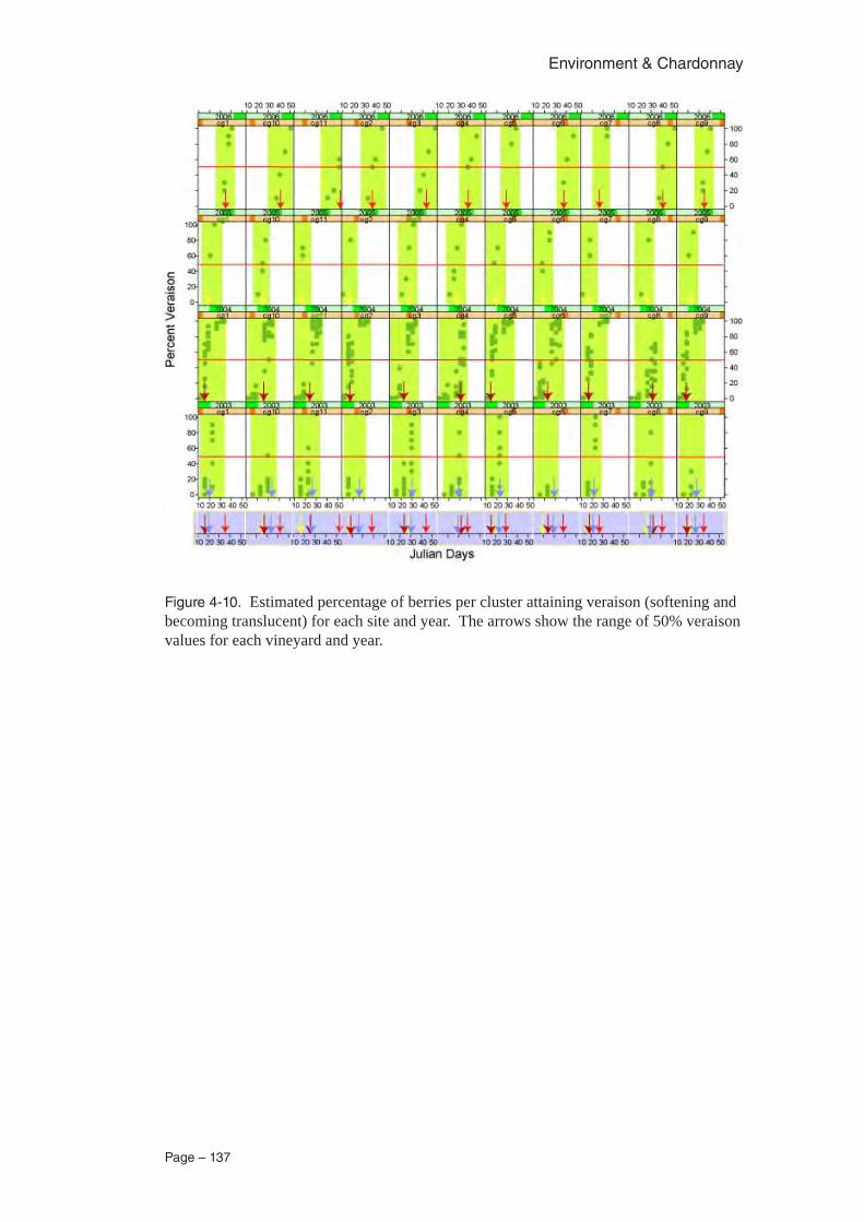
Page – 137
Environment & Chardonnay
Figure 4-10. Estimated percentage of berries per cluster attaining veraison (softening and becoming translucent) for each site and year. The arrows show the range of 50% veraison values for each vineyard and year.
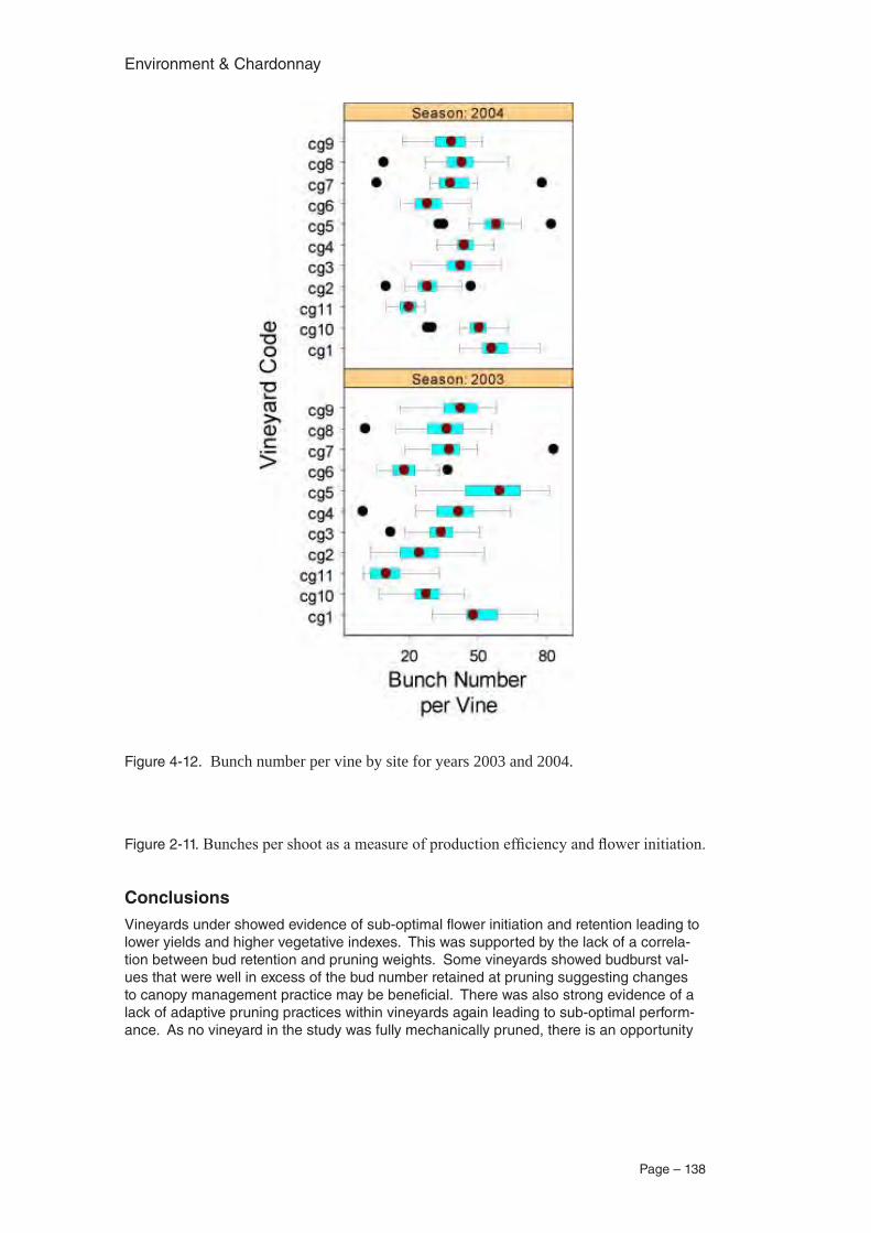
Environment & Chardonnay
Page – 138
Figure 4-12. Bunch number per vine by site for years 2003 and 2004.
Figure 2-11. Bunches per shoot as a measure of production efficiency and flower initiation.
ConclusionsVineyards under showed evidence of sub-optimal flower initiation and retention leading to lower yields and higher vegetative indexes. This was supported by the lack of a correla-tion between bud retention and pruning weights. Some vineyards showed budburst val-ues that were well in excess of the bud number retained at pruning suggesting changes to canopy management practice may be beneficial. There was also strong evidence of a lack of adaptive pruning practices within vineyards again leading to sub-optimal perform-ance. As no vineyard in the study was fully mechanically pruned, there is an opportunity
Page – 139
Environment & Chardonnay
Updated 10 Nov 05
Chardonnay Project Operational Procedures
Chardonnay Project Standard Operational Procedures Reviewed: September 2005 To be Revised: July 2006
2
List of Activities 1. Occupational Health and Safety ............................................22. Chardonnay Project Vineyard Locations...............................33. Outline of seasonal activities.................................................44. Experimental Layout .............................................................55. Data entry formats.................................................................66. Operational Records............................................................ 127. Annual Records: Vine and Vineyard................................... 15
7.1. Bud Burst .................................................................... 15 7.2. Cap-fall ....................................................................... 16 7.3. Petiole Sampling ......................................................... 17 7.4. Vegetative Growth – ................................................... 18
(a) Shoot Count/Bunch Count....................................... 18 (b) Vine Geometry ........................................................ 19 (c) Leaf Area & Shoot Diameter................................... 20 (d) Remote Sensing....................................................... 21 (e) Light Environment .................................................. 23
7.5. Véraison ...................................................................... 24 7.6. Maturity Fruit Sampling .............................................. 25
(a) Fruit sampling ......................................................... 25 (b) Fruit Assessment ...... Error! Bookmark not defined.
7.7. Fruit Harvest ............................................................... 27 7.8. Yield Mapping ............................................................ 28 7.9. Pruning & Pruning Weights ........................................ 30 7.10. Bud Counts.............................................................. 31 7.11. Carbohydrate Reserve Measurement ....................... 32
1. Occupational Health and SafetyEach person conducting work for this project is required to be trained in the safe use of each item of equipment that may be used in the field. Staff and students carrying out duties for this project are required to wear appropriate clothing (clothing that protects against excessive exposure to UV radiation, and is durable), has sun screen available for their use, and wears full cover work boots or shoes (steel capped if working with heavy items). Cool drinking water must be available and a field first aid kit (and the personnel must be aware of the contents of that kit and understand their proper use). It is good practice for an individual to be accompanied where possible in vineyard sampling exercises. This is not strictly required unless for other reasons such as lifting or carrying out operations that are inherently risky. No individual may drive unaccompanied for a period of more than six hours total in one day.All staff and students must make their manager/supervisor aware of their program of activities beforehand and their time of commencement and estimated time of completion. If not returning to the workplace, must otherwise notify their manager of their safe return. Staff operating in isolated sites should carry a mobile phone (CDMA) or 2-way radio [permission to use the Selwyn network should be negotiated if adopting this option].
to improve labour training to optimise vine performance within a vineyard and from year to year.
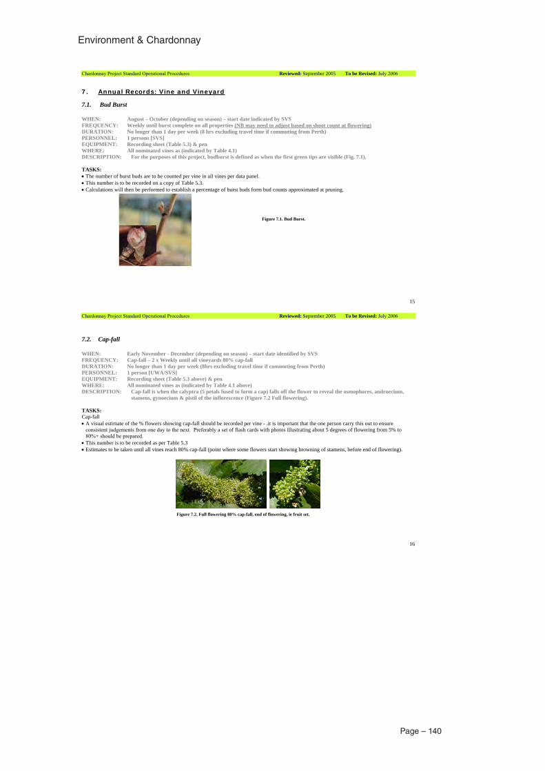
Environment & Chardonnay
Page – 140
Chardonnay Project Standard Operational Procedures Reviewed: September 2005 To be Revised: July 2006
15
Figure 7.1. Bud Burst.
7. Annual Records: Vine and Vineyard
7.1. Bud Burst
WHEN: August – October (depending on season) – start date indicated by SVS FREQUENCY: Weekly until burst complete on all properties (NB may need to adjust based on shoot count at flowering)DURATION: No longer than 1 day per week (8 hrs excluding travel time if commuting from Perth) PERSONNEL: 1 persons [SVS] EQUIPMENT: Recording sheet (Table 5.3) & pen WHERE: All nominated vines as (indicated by Table 4.1) DESCRIPTION: For the purposes of this project, budburst is defined as when the first green tips are visible (Fig. 7.1).
TASKS: The number of burst buds are to be counted per vine in all vines per data panel. This number is to be recorded on a copy of Table 5.3. Calculations will then be performed to establish a percentage of burst buds form bud counts approximated at pruning.
Chardonnay Project Standard Operational Procedures Reviewed: September 2005 To be Revised: July 2006
16
Figure 7.2. Full flowering 80% cap-fall, end of flowering, ie fruit set.
7.2. Cap-fall
WHEN: Early November - December (depending on season) – start date identified by SVS FREQUENCY: Cap-fall – 2 x Weekly until all vineyards 80% cap-fall DURATION: No longer than 1 day per week (8hrs excluding travel time if commuting from Perth) PERSONNEL: 1 person [UWA/SVS] EQUIPMENT: Recording sheet (Table 5.3 above) & pen WHERE: All nominated vines as (indicated by Table 4.1 above) DESCRIPTION: Cap-fall is when the calyptra (5 petals fused to form a cap) falls off the flower to reveal the osmophores, androecium,
stamens, gynoecium & pistil of the inflorescence (Figure 7.2 Full flowering).
TASKS: Cap-fall
A visual estimate of the % flowers showing cap-fall should be recorded per vine - .it is important that the one person carry this out to ensure consistent judgements from one day to the next. Preferably a set of flash cards with photos illustrating about 5 degrees of flowering from 5% to 80%+ should be prepared. This number is to be recorded as per Table 5.3 Estimates to be taken until all vines reach 80% cap-fall (point where some flowers start showing browning of stamens, before end of flowering).
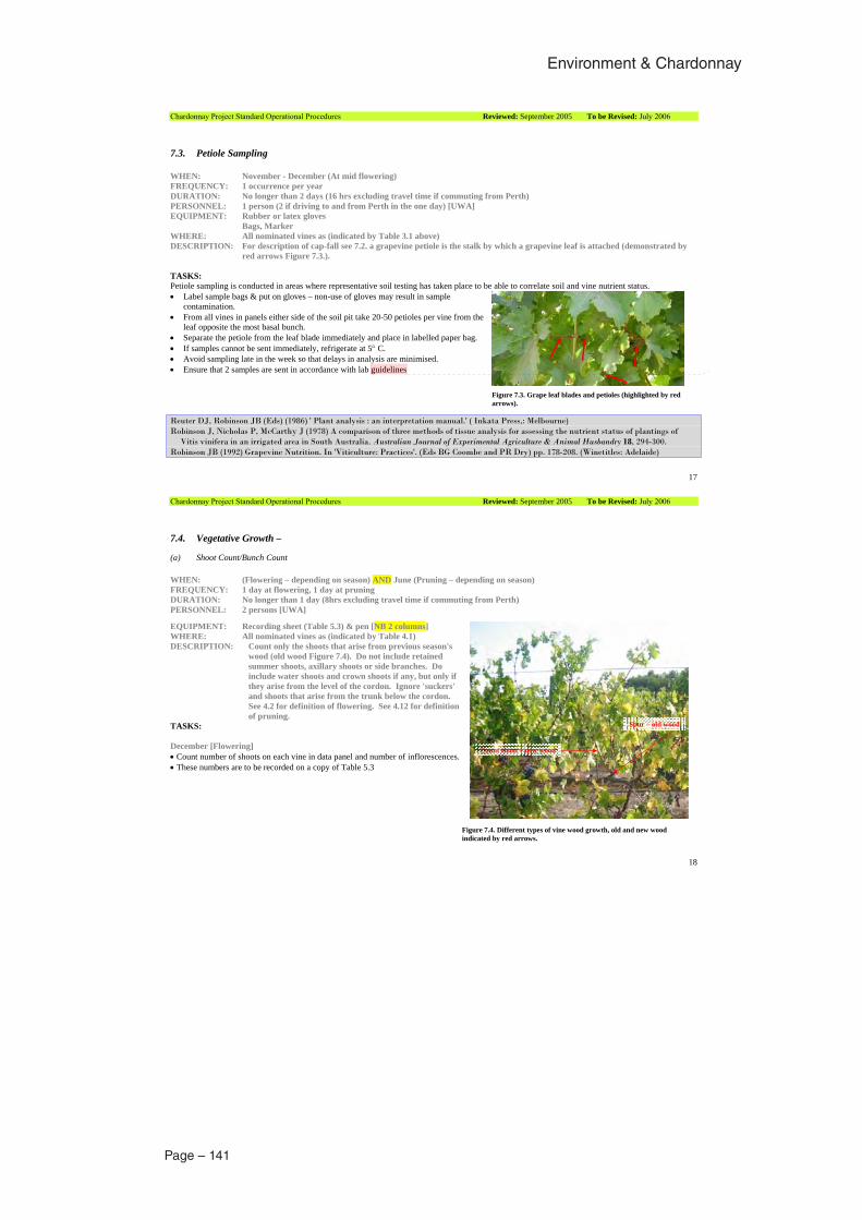
Page – 141
Environment & Chardonnay
Chardonnay Project Standard Operational Procedures Reviewed: September 2005 To be Revised: July 2006
17
Figure 7.3. Grape leaf blades and petioles (highlighted by red arrows).
7.3. Petiole Sampling
WHEN: November - December (At mid flowering) FREQUENCY: 1 occurrence per year DURATION: No longer than 2 days (16 hrs excluding travel time if commuting from Perth) PERSONNEL: 1 person (2 if driving to and from Perth in the one day) [UWA] EQUIPMENT: Rubber or latex gloves Bags, Marker WHERE: All nominated vines as (indicated by Table 3.1 above) DESCRIPTION: For description of cap-fall see 7.2. a grapevine petiole is the stalk by which a grapevine leaf is attached (demonstrated by
red arrows Figure 7.3.).
TASKS: Petiole sampling is conducted in areas where representative soil testing has taken place to be able to correlate soil and vine nutrient status.
Label sample bags & put on gloves – non-use of gloves may result in sample contamination. From all vines in panels either side of the soil pit take 20-50 petioles per vine from the leaf opposite the most basal bunch. Separate the petiole from the leaf blade immediately and place in labelled paper bag. If samples cannot be sent immediately, refrigerate at 5 C. Avoid sampling late in the week so that delays in analysis are minimised. Ensure that 2 samples are sent in accordance with lab guidelines
Reuter DJ, Robinson JB (Eds) (1986) ' Plant analysis : an interpretation manual.' ( Inkata Press,: Melbourne) Robinson J, Nicholas P, McCarthy J (1978) A comparison of three methods of tissue analysis for assessing the nutrient status of plantings of
Vitis vinifera in an irrigated area in South Australia. Australian Journal of Experimental Agriculture & Animal Husbandry 18, 294-300. Robinson JB (1992) Grapevine Nutrition. In 'Viticulture: Practices'. (Eds BG Coombe and PR Dry) pp. 178-208. (Winetitles: Adelaide)
Comment [jac1]: Jo what do you mean - Lab guidelines?
Chardonnay Project Standard Operational Procedures Reviewed: September 2005 To be Revised: July 2006
18
Count shoot – new wood
Spur – old wood
7.4. Vegetative Growth –
(a) Shoot Count/Bunch Count
WHEN: (Flowering – depending on season) AND June (Pruning – depending on season) FREQUENCY: 1 day at flowering, 1 day at pruning DURATION: No longer than 1 day (8hrs excluding travel time if commuting from Perth) PERSONNEL: 2 persons [UWA]
EQUIPMENT: Recording sheet (Table 5.3) & pen [NB 2 columns] WHERE: All nominated vines as (indicated by Table 4.1) DESCRIPTION: Count only the shoots that arise from previous season's
wood (old wood Figure 7.4). Do not include retained summer shoots, axillary shoots or side branches. Do include water shoots and crown shoots if any, but only if they arise from the level of the cordon. Ignore 'suckers' and shoots that arise from the trunk below the cordon. See 4.2 for definition of flowering. See 4.12 for definition of pruning.
TASKS:
December [Flowering] Count number of shoots on each vine in data panel and number of inflorescences. These numbers are to be recorded on a copy of Table 5.3
Figure 7.4. Different types of vine wood growth, old and new wood indicated by red arrows.
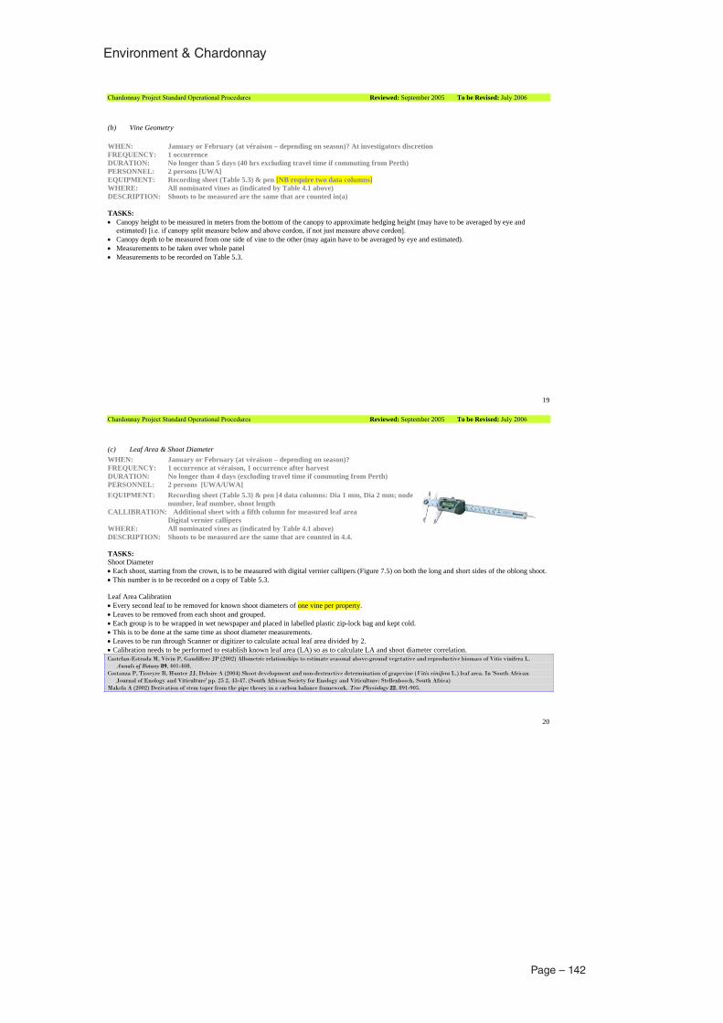
Environment & Chardonnay
Page – 142
Chardonnay Project Standard Operational Procedures Reviewed: September 2005 To be Revised: July 2006
19
(b) Vine Geometry
WHEN: January or February (at véraison – depending on season)? At investigators discretion FREQUENCY: 1 occurrence DURATION: No longer than 5 days (40 hrs excluding travel time if commuting from Perth) PERSONNEL: 2 persons [UWA] EQUIPMENT: Recording sheet (Table 5.3) & pen [NB require two data columns] WHERE: All nominated vines as (indicated by Table 4.1 above) DESCRIPTION: Shoots to be measured are the same that are counted in(a)
TASKS: Canopy height to be measured in meters from the bottom of the canopy to approximate hedging height (may have to be averaged by eye and estimated) [i.e. if canopy split measure below and above cordon, if not just measure above cordon]. Canopy depth to be measured from one side of vine to the other (may again have to be averaged by eye and estimated). Measurements to be taken over whole panel Measurements to be recorded on Table 5.3.
Chardonnay Project Standard Operational Procedures Reviewed: September 2005 To be Revised: July 2006
20
(c) Leaf Area & Shoot Diameter WHEN: January or February (at véraison – depending on season)? FREQUENCY: 1 occurrence at véraison, 1 occurrence after harvest DURATION: No longer than 4 days (excluding travel time if commuting from Perth) PERSONNEL: 2 persons [UWA/UWA] EQUIPMENT: Recording sheet (Table 5.3) & pen [4 data columns: Dia 1 mm, Dia 2 mm; node
number, leaf number, shoot length CALLIBRATION: Additional sheet with a fifth column for measured leaf area Digital vernier callipers WHERE: All nominated vines as (indicated by Table 4.1 above) DESCRIPTION: Shoots to be measured are the same that are counted in 4.4.
TASKS: Shoot Diameter
Each shoot, starting from the crown, is to be measured with digital vernier callipers (Figure 7.5) on both the long and short sides of the oblong shoot. This number is to be recorded on a copy of Table 5.3.
Leaf Area Calibration Every second leaf to be removed for known shoot diameters of one vine per property. Leaves to be removed from each shoot and grouped. Each group is to be wrapped in wet newspaper and placed in labelled plastic zip-lock bag and kept cold. This is to be done at the same time as shoot diameter measurements. Leaves to be run through Scanner or digitizer to calculate actual leaf area divided by 2. Calibration needs to be performed to establish known leaf area (LA) so as to calculate LA and shoot diameter correlation.
Castelan-Estrada M, Vivin P, Gaudillere JP (2002) Allometric relationships to estimate seasonal above-ground vegetative and reproductive biomass of Vitis vinifera L. Annals of Botany 89, 401-408.
Costanza P, Tisseyre B, Hunter JJ, Deloire A (2004) Shoot development and non-destructive determination of grapevine (Vitis vinifera L.) leaf area. In 'South African Journal of Enology and Viticulture' pp. 25 2, 43-47. (South African Society for Enology and Viticulture: Stellenbosch, South Africa)
Makela A (2002) Derivation of stem taper from the pipe theory in a carbon balance framework. Tree Physiology 22, 891-905.
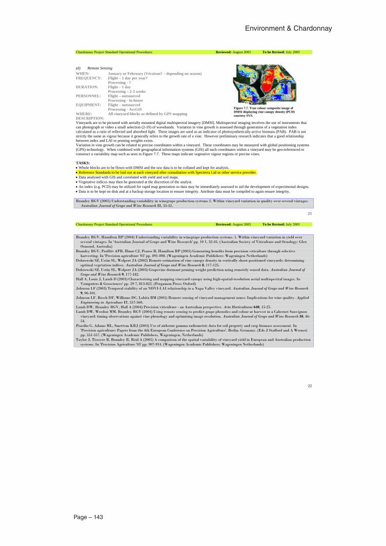
Page – 143
Environment & Chardonnay
Chardonnay Project Standard Operational Procedures Reviewed: August 2005 To be Revised: July 2005
21
(d) Remote Sensing WHEN: January or February (Véraison? – depending on season) FREQUENCY: Flight – 1 day per year? Processing - ? DURATION: Flight – 1 day Processing – 2-3 weeks PERSONNEL: Flight – outsourced Processing - in-house EQUIPMENT: Flight – outsourced Processing - ArcGIS WHERE: All vineyard blocks as defined by GPS mapping DESCRIPTION:Vineyards are to be pictured with aerially mounted digital multispectral imagery [DMSI]. Multispectral imaging involves the use of instruments that can photograph or video a small selection (2-10) of wavebands. Variation in vine growth is assessed through generation of a vegetation index calculated as a ratio of reflected and absorbed light. These images are used as an indicator of photosynthetically-active biomass (PAB). PAB is not strictly the same as vigour because it generally refers to the growth rate of a vine. However preliminary research indicates that a good relationship between index and LAI or pruning weights exists. Variation in vine growth can be related to precise coordinates within a vineyard. These coordinates may be measured with global positioning systems (GPS) technology. When combined with geographical information systems (GIS) all such coordinates within a vineyard may be geo-referenced to construct a variability map such as seen in Figure 7.7. These maps indicate vegetative vigour regions or precise vines.
TASKS: Whole blocks are to be flown with DMSI and the raw data is to be collated and kept for analysis. Reference Standards to be laid out at each vineyard after consultation with Specterra Ltd or other service provider. Data analysed with GIS and correlated with yield and soil maps. Vegetative indices may then be generated at the discretion of the analyst. An index (e.g. PCD) may be utilized for rapid map generation so data may be immediately assessed to aid the development of experimental designs. Data is to be kept on disk and at a backup storage location to ensure integrity. Attribute data must be compiled to again ensure integrity.
Bramley RGV (2005) Understanding variability in winegrape production systems 2. Within vineyard variation in quality over several vintages. Australian Journal of Grape and Wine Research 11, 33-42.
Figure 7.7. True colour composite image of DMSI displaying cine canopy density (PCD) courtesy SVS.
Chardonnay Project Standard Operational Procedures Reviewed: August 2005 To be Revised: July 2005
22
Bramley RGV, Hamilton RP (2004) Understanding variability in winegrape production systems. 1. Within vineyard variation in yield over several vintages. In 'Australian Journal of Grape and Wine Research' pp. 10 1, 32-45. (Australian Society of Viticulture and Oenology: Glen Osmond, Australia)
Bramley RGV, Proffitt APB, Hinze CJ, Pearse B, Hamilton RP (2005) Generating benefits from precision viticulture through selective harvesting. In 'Precision agriculture '05' pp. 891-898. (Wageningen Academic Publishers: Wageningen Netherlands)
Dobrowski SZ, Ustin SL, Wolpert JA (2002) Remote estimation of vine canopy density in vertically shoot-positioned vineyards: determining optimal vegetation indices. Australian Journal of Grape and Wine Research 8, 117-125.
Dobrowski SZ, Ustin SL, Wolpert JA (2003) Grapevine dormant pruning weight prediction using remotely sensed data. Australian Journal of Grape and Wine Research 9, 177-182.
Hall A, Louis J, Lamb D (2003) Characterising and mapping vineyard canopy using high-spatial-resolution aerial multispectral images. In 'Computers & Geosciences' pp. 29 7, 813-822. (Pergamon Press: Oxford)
Johnson LF (2003) Temporal stability of an NDVI-LAI relationship in a Napa Valley vineyard. Australian Journal of Grape and Wine Research9, 96-101.
Johnson LF, Bosch DF, Williams DC, Lobitz BM (2001) Remote sensing of vineyard management zones: Implications for wine quality. AppliedEngineering in Agriculture 17, 557-560.
Lamb DW, Bramley RGV, Hall A (2004) Precision viticulture - an Australian perspective. Acta Horticulturae 640, 15-25. Lamb DW, Weedon MM, Bramley RGV (2004) Using remote sensing to predict grape phenolics and colour at harvest in a Cabernet Sauvignon
vineyard: timing observations against vine phenology and optimising image resolution. Australian Journal of Grape and Wine Research 10, 46-54.
Pracilio G, Adams ML, Smettem KRJ (2003) Use of airborne gamma radiometric data for soil property and crop biomass assessment. In'Precision agriculture: Papers from the 4th European Conference on Precision Agriculture'. Berlin, Germany. (Eds J Stafford and A Werner) pp. 551-557. (Wageningen Academic Publishers, Wageningen, Netherlands)
Taylor J, Tisseyre B, Bramley R, Reid A (2005) A comparison of the spatial variability of vineyard yield in European and Australian production systems. In 'Precision Agriculture '05' pp. 907-914. (Wageningen Academic Publishers: Wageningen Netherlands)
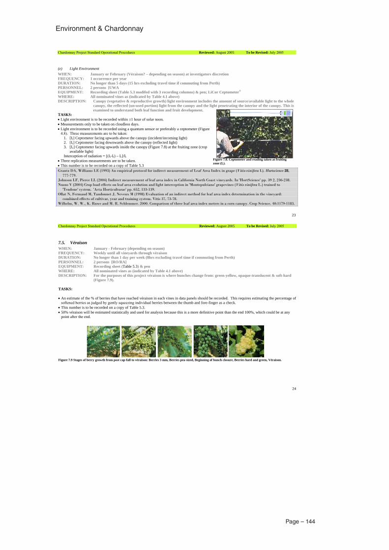
Environment & Chardonnay
Page – 144
Chardonnay Project Standard Operational Procedures Reviewed: August 2005 To be Revised: July 2005
23
(e) Light Environment WHEN: January or February (Véraison? – depending on season) at investigators discretion FREQUENCY: 1 occurrence per year DURATION: No longer than 5 days (15 hrs excluding travel time if commuting from Perth) PERSONNEL: 2 persons [UWA EQUIPMENT: Recording sheet (Table 5.3 modifed with 3 recording columns) & pen; LiCor Ceptometer®
WHERE: All nominated vines as (indicated by Table 4.1 above) DESCRIPTION: Canopy (vegetative & reproductive growth) light environment includes the amount of source/available light to the whole
canopy, the reflected (un-used portion) light from the canopy and the light penetrating the interior of the canopy. This is examined to understand both leaf function and fruit development.
TASKS: Light environment is to be recorded within ±1 hour of solar noon. Measurements only to be taken on cloudless days. Light environment is to be recorded using a quantum sensor or preferably a ceptometer (Figure 4.8). Three measurements are to be taken:
1. [Ii] Ceptometer facing upwards above the canopy (incident/incoming light) 2. [Ir] Ceptometer facing downwards above the canopy (reflected light) 3. [Ic] Ceptometer facing upwards inside the canopy (Figure 7.8) at the fruiting zone (crop
available light) Interception of radiation = [(Ii-Ir) – Ic]/Ii
Three replication measurements are to be taken. This number is to be recorded on a copy of Table 5.3
Grantz DA, Williams LE (1993) An empirical protocol for indirect measurement of Leaf Area Index in grape (Vitis-vinifera L). Hortscience 28,777-779.
Johnson LF, Pierce LL (2004) Indirect measurement of leaf area index in California North Coast vineyards. In 'HortScience' pp. 39 2, 236-238. Nuzzo V (2004) Crop load effects on leaf area evolution and light interception in 'Montepulciano' grapevines (Vitis vinifera L.) trained to
'Tendone' system. 'Acta Horticulturae' pp. 652, 133-139. Ollat N, Fermaud M, Tandonnet J, Neveux M (1998) Evaluation of an indirect method for leaf area index determination in the vineyard:
combined effects of cultivar, year and training system. Vitis 37, 73-78. Wilhelm, W. W., K. Ruwe and M. R. Schlemmer. 2000. Comparison of three leaf area index meters in a corn canopy. Crop Science. 40:1179-1183.
Figure 7.8. Ceptometer and reading taken at fruiting zone (Ic).
Chardonnay Project Standard Operational Procedures Reviewed: August 2005 To be Revised: July 2005
24
7.5. Véraison WHEN: January - February (depending on season) FREQUENCY: Weekly until all vineyards through véraison DURATION: No longer than 1 day per week (8hrs excluding travel time if commuting from Perth) PERSONNEL: 2 persons [RO/RA] EQUIPMENT: Recording sheet (Table 5.3) & pen WHERE: All nominated vines as (indicated by Table 4.1 above) DESCRIPTION: For the purposes of this project véraison is where bunches change from: green-yellow, opaque-translucent & soft-hard
(Figure 7.9).
TASKS:
An estimate of the % of berries that have reached véraison in each vines in data panels should be recorded. This requires estimating the percentage of softened berries as judged by gently squeezing individual berries between the thumb and fore-finger as a check. This number is to be recorded on a copy of Table 5.3. 50% véraison will be estimated statistically and used for analysis because this is a more definitive point than the end 100%, which could be at any point after the end.
Figure 7.9 Stages of berry growth from post cap-fall to véraison: Berries 3 mm, Berries pea-sized, Beginning of bunch closure, Berries hard and green, Véraison.
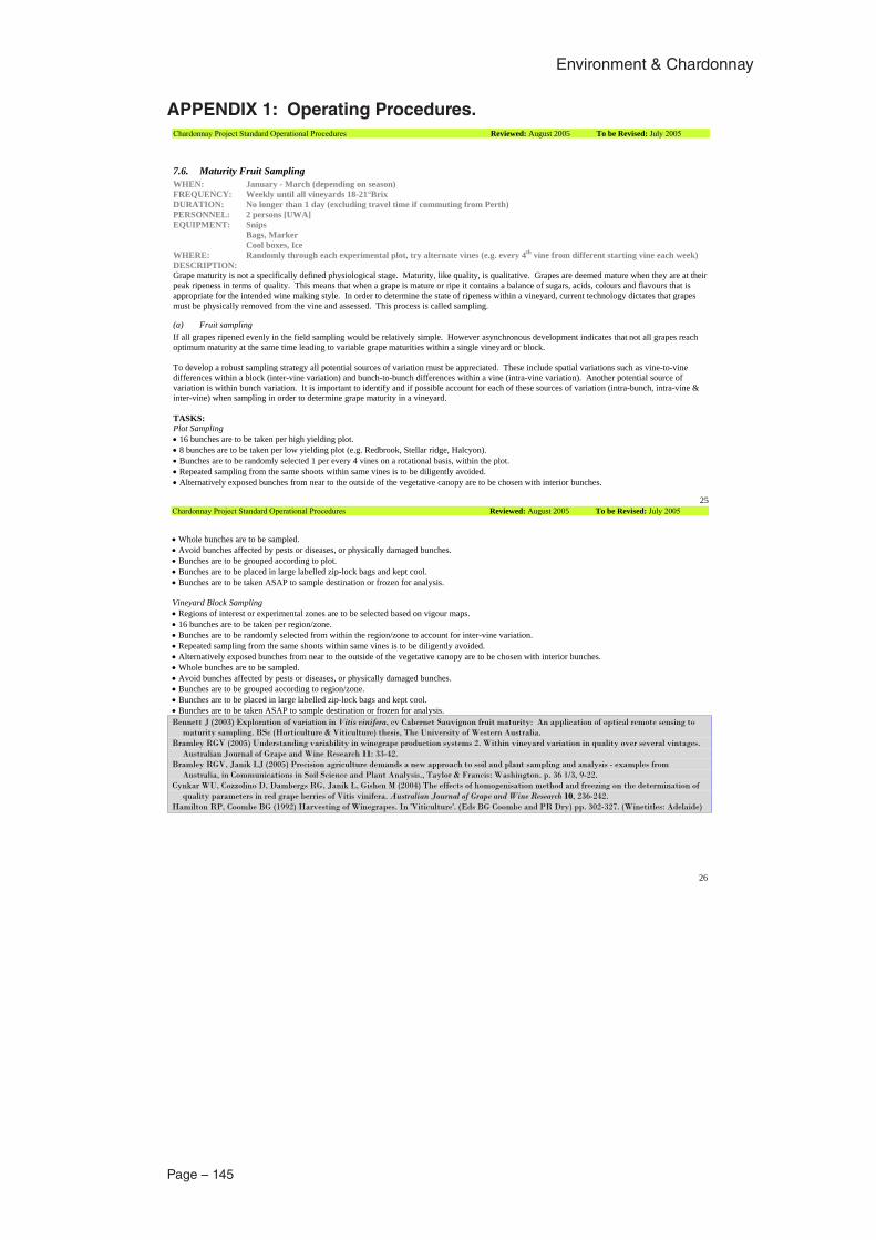
Page – 145
Environment & Chardonnay
APPENDIX 1: Operating Procedures.Chardonnay Project Standard Operational Procedures Reviewed: August 2005 To be Revised: July 2005
25
7.6. Maturity Fruit Sampling WHEN: January - March (depending on season) FREQUENCY: Weekly until all vineyards 18-21°Brix DURATION: No longer than 1 day (excluding travel time if commuting from Perth) PERSONNEL: 2 persons [UWA] EQUIPMENT: Snips Bags, Marker Cool boxes, Ice WHERE: Randomly through each experimental plot, try alternate vines (e.g. every 4th vine from different starting vine each week) DESCRIPTION: Grape maturity is not a specifically defined physiological stage. Maturity, like quality, is qualitative. Grapes are deemed mature when they are at their peak ripeness in terms of quality. This means that when a grape is mature or ripe it contains a balance of sugars, acids, colours and flavours that is appropriate for the intended wine making style. In order to determine the state of ripeness within a vineyard, current technology dictates that grapes must be physically removed from the vine and assessed. This process is called sampling.
(a) Fruit sampling If all grapes ripened evenly in the field sampling would be relatively simple. However asynchronous development indicates that not all grapes reach optimum maturity at the same time leading to variable grape maturities within a single vineyard or block.
To develop a robust sampling strategy all potential sources of variation must be appreciated. These include spatial variations such as vine-to-vine differences within a block (inter-vine variation) and bunch-to-bunch differences within a vine (intra-vine variation). Another potential source of variation is within bunch variation. It is important to identify and if possible account for each of these sources of variation (intra-bunch, intra-vine & inter-vine) when sampling in order to determine grape maturity in a vineyard.
TASKS: Plot Sampling
16 bunches are to be taken per high yielding plot. 8 bunches are to be taken per low yielding plot (e.g. Redbrook, Stellar ridge, Halcyon). Bunches are to be randomly selected 1 per every 4 vines on a rotational basis, within the plot. Repeated sampling from the same shoots within same vines is to be diligently avoided. Alternatively exposed bunches from near to the outside of the vegetative canopy are to be chosen with interior bunches.
Chardonnay Project Standard Operational Procedures Reviewed: August 2005 To be Revised: July 2005
26
Whole bunches are to be sampled. Avoid bunches affected by pests or diseases, or physically damaged bunches. Bunches are to be grouped according to plot. Bunches are to be placed in large labelled zip-lock bags and kept cool. Bunches are to be taken ASAP to sample destination or frozen for analysis.
Vineyard Block Sampling Regions of interest or experimental zones are to be selected based on vigour maps. 16 bunches are to be taken per region/zone. Bunches are to be randomly selected from within the region/zone to account for inter-vine variation. Repeated sampling from the same shoots within same vines is to be diligently avoided. Alternatively exposed bunches from near to the outside of the vegetative canopy are to be chosen with interior bunches. Whole bunches are to be sampled. Avoid bunches affected by pests or diseases, or physically damaged bunches. Bunches are to be grouped according to region/zone. Bunches are to be placed in large labelled zip-lock bags and kept cool. Bunches are to be taken ASAP to sample destination or frozen for analysis.
Bennett J (2003) Exploration of variation in Vitis vinifera, cv Cabernet Sauvignon fruit maturity: An application of optical remote sensing to maturity sampling. BSc (Horticulture & Viticulture) thesis, The University of Western Australia.
Bramley RGV (2005) Understanding variability in winegrape production systems 2. Within vineyard variation in quality over several vintages. Australian Journal of Grape and Wine Research 11: 33-42.
Bramley RGV, Janik LJ (2005) Precision agriculture demands a new approach to soil and plant sampling and analysis - examples from Australia, in Communications in Soil Science and Plant Analysis., Taylor & Francis: Washington. p. 36 1/3, 9-22.
Cynkar WU, Cozzolino D, Dambergs RG, Janik L, Gishen M (2004) The effects of homogenisation method and freezing on the determination of quality parameters in red grape berries of Vitis vinifera. Australian Journal of Grape and Wine Research 10, 236-242.
Hamilton RP, Coombe BG (1992) Harvesting of Winegrapes. In 'Viticulture'. (Eds BG Coombe and PR Dry) pp. 302-327. (Winetitles: Adelaide)
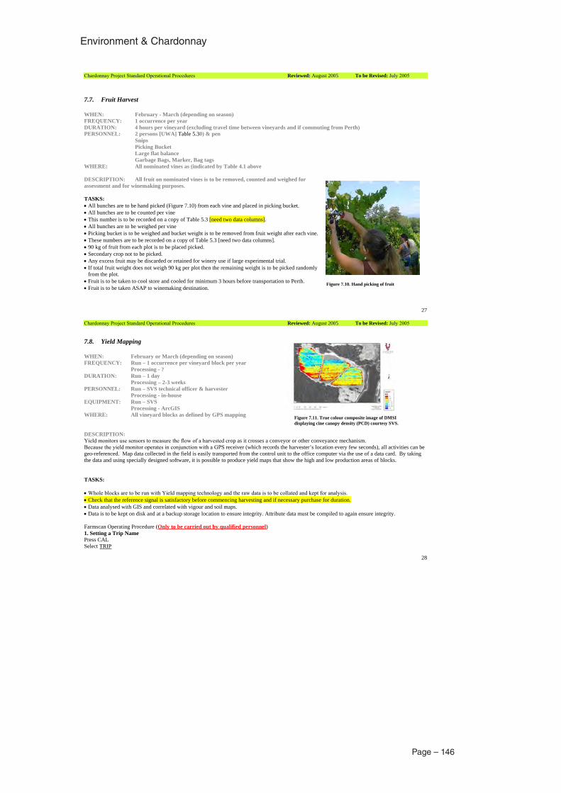
Environment & Chardonnay
Page – 146
Chardonnay Project Standard Operational Procedures Reviewed: August 2005 To be Revised: July 2005
27
7.7. Fruit Harvest
WHEN: February - March (depending on season) FREQUENCY: 1 occurrence per year DURATION: 4 hours per vineyard (excluding travel time between vineyards and if commuting from Perth) PERSONNEL: 2 persons [UWA] Table 5.30) & pen Snips Picking Bucket Large flat balance Garbage Bags, Marker, Bag tags WHERE: All nominated vines as (indicated by Table 4.1 above
DESCRIPTION: All fruit on nominated vines is to be removed, counted and weighed for assessment and for winemaking purposes.
TASKS: All bunches are to be hand picked (Figure 7.10) from each vine and placed in picking bucket. All bunches are to be counted per vine This number is to be recorded on a copy of Table 5.3 [need two data columns]. All bunches are to be weighed per vine Picking bucket is to be weighed and bucket weight is to be removed from fruit weight after each vine. These numbers are to be recorded on a copy of Table 5.3 [need two data columns]. 90 kg of fruit from each plot is to be placed picked. Secondary crop not to be picked. Any excess fruit may be discarded or retained for winery use if large experimental trial. If total fruit weight does not weigh 90 kg per plot then the remaining weight is to be picked randomly from the plot. Fruit is to be taken to cool store and cooled for minimum 3 hours before transportation to Perth. Fruit is to be taken ASAP to winemaking destination.
Figure 7.10. Hand picking of fruit
Chardonnay Project Standard Operational Procedures Reviewed: August 2005 To be Revised: July 2005
28
7.8. Yield Mapping
WHEN: February or March (depending on season) FREQUENCY: Run – 1 occurrence per vineyard block per year Processing - ? DURATION: Run – 1 day Processing – 2-3 weeks PERSONNEL: Run – SVS technical officer & harvester Processing - in-house EQUIPMENT: Run – SVS Processing - ArcGIS WHERE: All vineyard blocks as defined by GPS mapping
DESCRIPTION:Yield monitors use sensors to measure the flow of a harvested crop as it crosses a conveyor or other conveyance mechanism. Because the yield monitor operates in conjunction with a GPS receiver (which records the harvester’s location every few seconds), all activities can be geo-referenced. Map data collected in the field is easily transported from the control unit to the office computer via the use of a data card. By taking the data and using specially designed software, it is possible to produce yield maps that show the high and low production areas of blocks.
TASKS:
Whole blocks are to be run with Yield mapping technology and the raw data is to be collated and kept for analysis. Check that the reference signal is satisfactory before commencing harvesting and if necessary purchase for duration. Data analysed with GIS and correlated with vigour and soil maps. Data is to be kept on disk and at a backup storage location to ensure integrity. Attribute data must be compiled to again ensure integrity.
Farmscan Operating Procedure (Only to be carried out by qualified personnel)1. Setting a Trip Name Press CAL Select TRIP
Figure 7.11. True colour composite image of DMSI displaying cine canopy density (PCD) courtesy SVS.
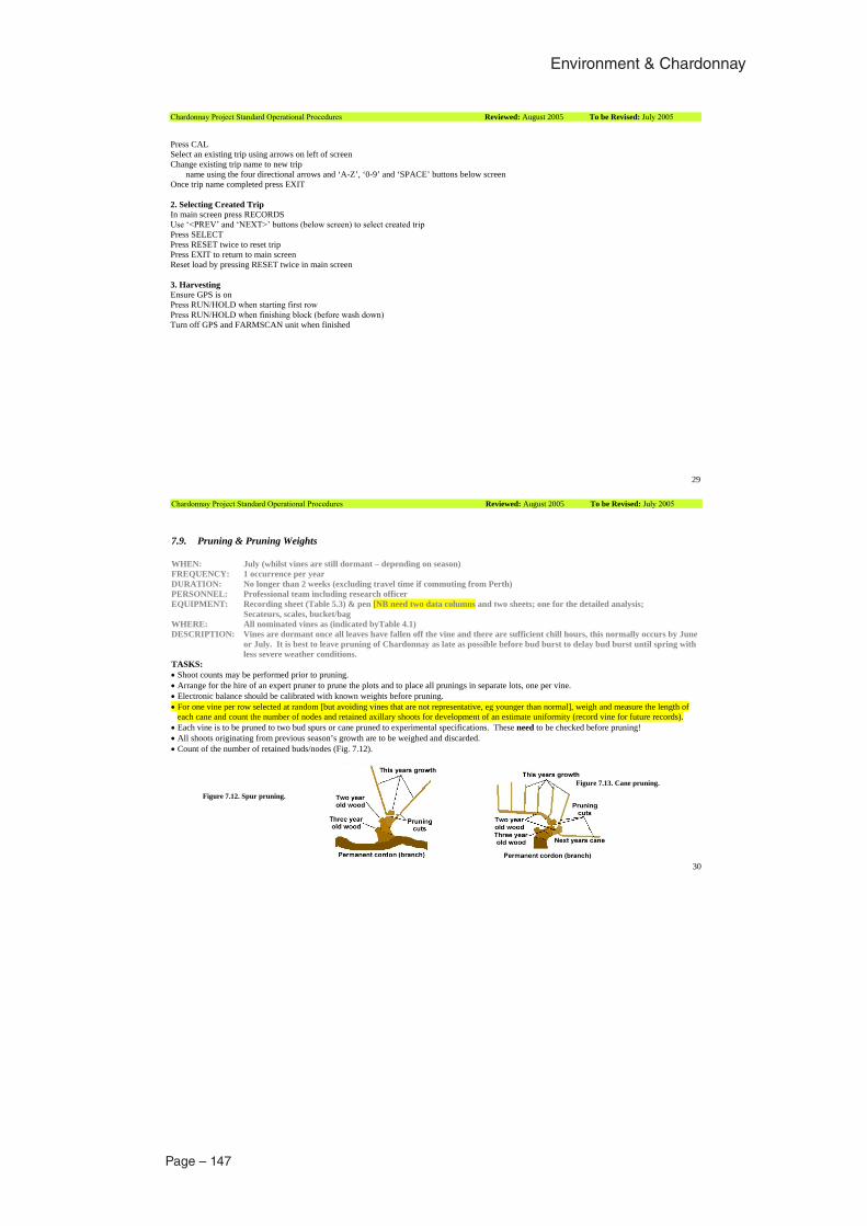
Page – 147
Environment & Chardonnay
Chardonnay Project Standard Operational Procedures Reviewed: August 2005 To be Revised: July 2005
29
Press CAL Select an existing trip using arrows on left of screen Change existing trip name to new trip name using the four directional arrows and ‘A-Z’, ‘0-9’ and ‘SPACE’ buttons below screen Once trip name completed press EXIT
2. Selecting Created Trip In main screen press RECORDSUse ‘<PREV’ and ‘NEXT>’ buttons (below screen) to select created tripPress SELECTPress RESET twice to reset tripPress EXIT to return to main screenReset load by pressing RESET twice in main screen
3. Harvesting Ensure GPS is onPress RUN/HOLD when starting first rowPress RUN/HOLD when finishing block (before wash down)Turn off GPS and FARMSCAN unit when finished
Chardonnay Project Standard Operational Procedures Reviewed: August 2005 To be Revised: July 2005
30
7.9. Pruning & Pruning Weights
WHEN: July (whilst vines are still dormant – depending on season) FREQUENCY: 1 occurrence per year DURATION: No longer than 2 weeks (excluding travel time if commuting from Perth) PERSONNEL: Professional team including research officer EQUIPMENT: Recording sheet (Table 5.3) & pen [NB need two data columns and two sheets; one for the detailed analysis; Secateurs, scales, bucket/bag WHERE: All nominated vines as (indicated byTable 4.1) DESCRIPTION: Vines are dormant once all leaves have fallen off the vine and there are sufficient chill hours, this normally occurs by June
or July. It is best to leave pruning of Chardonnay as late as possible before bud burst to delay bud burst until spring with less severe weather conditions.
TASKS: Shoot counts may be performed prior to pruning. Arrange for the hire of an expert pruner to prune the plots and to place all prunings in separate lots, one per vine. Electronic balance should be calibrated with known weights before pruning. For one vine per row selected at random [but avoiding vines that are not representative, eg younger than normal], weigh and measure the length of each cane and count the number of nodes and retained axillary shoots for development of an estimate uniformity (record vine for future records). Each vine is to be pruned to two bud spurs or cane pruned to experimental specifications. These need to be checked before pruning! All shoots originating from previous season’s growth are to be weighed and discarded. Count of the number of retained buds/nodes (Fig. 7.12).
Figure 7.12. Spur pruning.
Figure 7.13. Cane pruning.
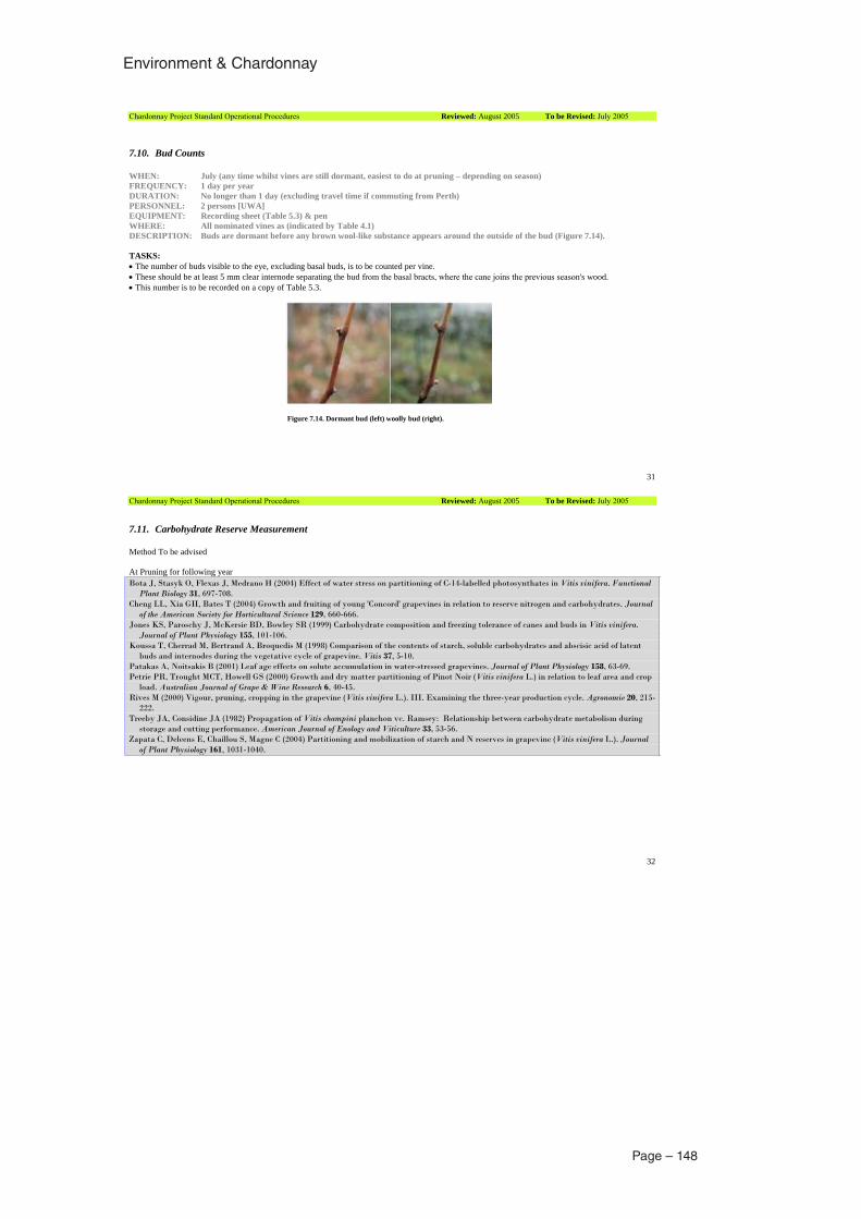
Environment & Chardonnay
Page – 148
Chardonnay Project Standard Operational Procedures Reviewed: August 2005 To be Revised: July 2005
31
Figure 7.14. Dormant bud (left) woolly bud (right).
7.10. Bud Counts
WHEN: July (any time whilst vines are still dormant, easiest to do at pruning – depending on season) FREQUENCY: 1 day per year DURATION: No longer than 1 day (excluding travel time if commuting from Perth) PERSONNEL: 2 persons [UWA] EQUIPMENT: Recording sheet (Table 5.3) & pen WHERE: All nominated vines as (indicated by Table 4.1) DESCRIPTION: Buds are dormant before any brown wool-like substance appears around the outside of the bud (Figure 7.14).
TASKS: The number of buds visible to the eye, excluding basal buds, is to be counted per vine. These should be at least 5 mm clear internode separating the bud from the basal bracts, where the cane joins the previous season's wood. This number is to be recorded on a copy of Table 5.3.
Chardonnay Project Standard Operational Procedures Reviewed: August 2005 To be Revised: July 2005
32
7.11. Carbohydrate Reserve Measurement
Method To be advised
At Pruning for following year Bota J, Stasyk O, Flexas J, Medrano H (2004) Effect of water stress on partitioning of C-14-labelled photosynthates in Vitis vinifera. Functional
Plant Biology 31, 697-708. Cheng LL, Xia GH, Bates T (2004) Growth and fruiting of young 'Concord' grapevines in relation to reserve nitrogen and carbohydrates. Journal
of the American Society for Horticultural Science 129, 660-666. Jones KS, Paroschy J, McKersie BD, Bowley SR (1999) Carbohydrate composition and freezing tolerance of canes and buds in Vitis vinifera.
Journal of Plant Physiology 155, 101-106. Koussa T, Cherrad M, Bertrand A, Broquedis M (1998) Comparison of the contents of starch, soluble carbohydrates and abscisic acid of latent
buds and internodes during the vegetative cycle of grapevine. Vitis 37, 5-10. Patakas A, Noitsakis B (2001) Leaf age effects on solute accumulation in water-stressed grapevines. Journal of Plant Physiology 158, 63-69. Petrie PR, Trought MCT, Howell GS (2000) Growth and dry matter partitioning of Pinot Noir (Vitis vinifera L.) in relation to leaf area and crop
load. Australian Journal of Grape & Wine Research 6, 40-45. Rives M (2000) Vigour, pruning, cropping in the grapevine (Vitis vinifera L.). III. Examining the three-year production cycle. Agronomie 20, 215-
222. Treeby JA, Considine JA (1982) Propagation of Vitis champini planchon vc. Ramsey: Relationship between carbohydrate metabolism during
storage and cutting performance. American Journal of Enology and Viticulture 33, 53-56. Zapata C, Deleens E, Chaillou S, Magne C (2004) Partitioning and mobilization of starch and N reserves in grapevine (Vitis vinifera L.). Journal
of Plant Physiology 161, 1031-1040.

Page – 149
Environment & Chardonnay
Chardonnay Project Standard Operational Procedures Reviewed: August 2005 To be Revised: July 2005
33
8. Version Changes10/11/05 Allometry references updated – note procedure may need to change to reflect published information.
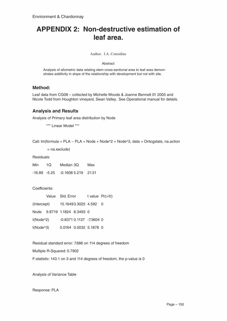
Environment & Chardonnay
Page – 150
APPENDIX 2: Non-destructive estimation of leaf area.
Author. J.A. Considine
Abstract
Analysis of allometric data relating stem cross-sectional area to leaf area demon-strates additivity in slope of the relationship with development but not with site.
Method: Leaf data from CG08 – collected by Michelle Woods & Joanne Bennett 01 2005 and Nicole Todd from Houghton vineyard, Swan Valley. See Operational manual for details.
Analysis and ResultsAnalysis of Primary leaf area distribution by Node
*** Linear Model ***
Call: lm(formula = PLA ~ PLA + Node + Node^2 + Node^3, data = Ontogstats, na.action
= na.exclude)
Residuals:
Min 1Q Median 3Q Max
-16.89 -5.25 -0.1608 5.219 21.31
Coefficients:
Value Std. Error t value Pr(>|t|)
(Intercept) 15.1649 3.3025 4.592 0
Node 9.8719 1.1824 8.3493 0
I(Node^2) -0.8371 0.1137 -7.3604 0
I(Node^3) 0.0164 0.0032 5.1878 0
Residual standard error: 7.686 on 114 degrees of freedom
Multiple R-Squared: 0.7902
F-statistic: 143.1 on 3 and 114 degrees of freedom, the p-value is 0
Analysis of Variance Table
Response: PLA
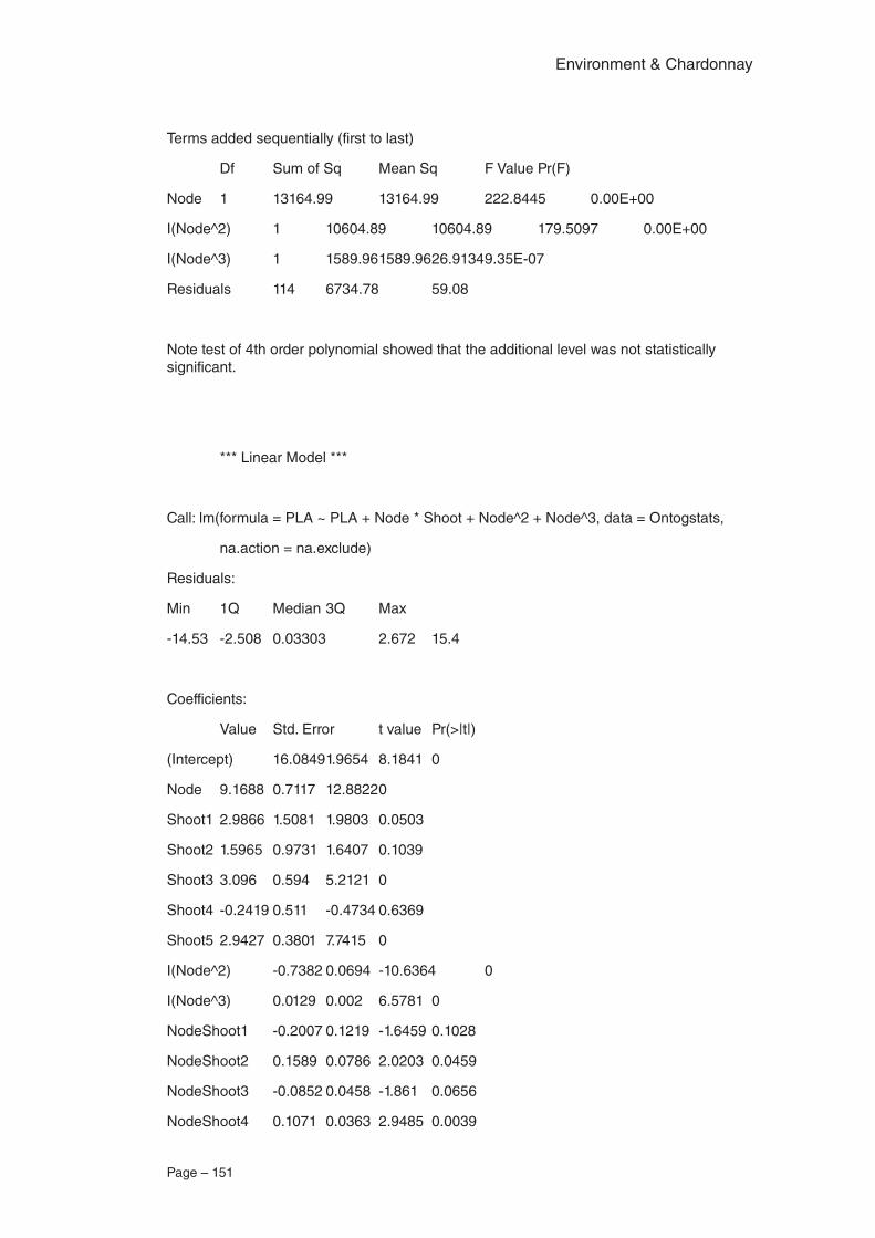
Page – 151
Environment & Chardonnay
Terms added sequentially (first to last)
Df Sum of Sq Mean Sq F Value Pr(F)
Node 1 13164.99 13164.99 222.8445 0.00E+00
I(Node^2) 1 10604.89 10604.89 179.5097 0.00E+00
I(Node^3) 1 1589.96 1589.96 26.9134 9.35E-07
Residuals 114 6734.78 59.08
Note test of 4th order polynomial showed that the additional level was not statistically significant.
*** Linear Model ***
Call: lm(formula = PLA ~ PLA + Node * Shoot + Node^2 + Node^3, data = Ontogstats,
na.action = na.exclude)
Residuals:
Min 1Q Median 3Q Max
-14.53 -2.508 0.03303 2.672 15.4
Coefficients:
Value Std. Error t value Pr(>|t|)
(Intercept) 16.0849 1.9654 8.1841 0
Node 9.1688 0.7117 12.8822 0
Shoot1 2.9866 1.5081 1.9803 0.0503
Shoot2 1.5965 0.9731 1.6407 0.1039
Shoot3 3.096 0.594 5.2121 0
Shoot4 -0.2419 0.511 -0.4734 0.6369
Shoot5 2.9427 0.3801 7.7415 0
I(Node^2) -0.7382 0.0694 -10.6364 0
I(Node^3) 0.0129 0.002 6.5781 0
NodeShoot1 -0.2007 0.1219 -1.6459 0.1028
NodeShoot2 0.1589 0.0786 2.0203 0.0459
NodeShoot3 -0.0852 0.0458 -1.861 0.0656
NodeShoot4 0.1071 0.0363 2.9485 0.0039
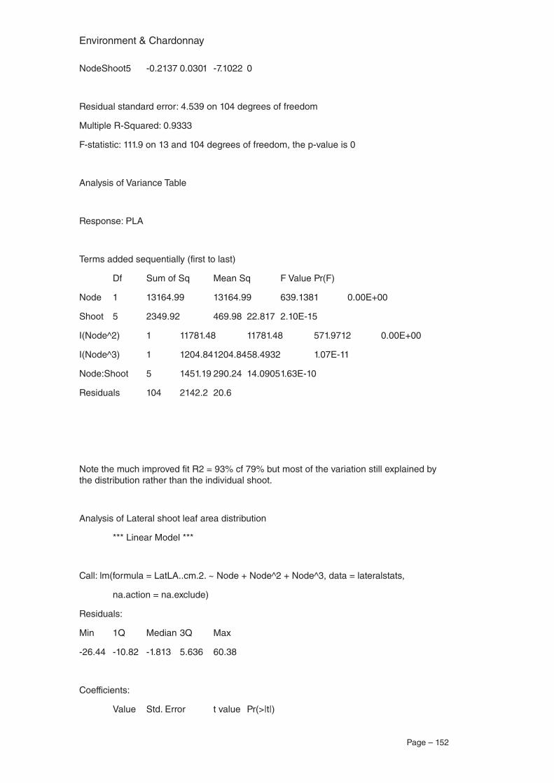
Environment & Chardonnay
Page – 152
NodeShoot5 -0.2137 0.0301 -7.1022 0
Residual standard error: 4.539 on 104 degrees of freedom
Multiple R-Squared: 0.9333
F-statistic: 111.9 on 13 and 104 degrees of freedom, the p-value is 0
Analysis of Variance Table
Response: PLA
Terms added sequentially (first to last)
Df Sum of Sq Mean Sq F Value Pr(F)
Node 1 13164.99 13164.99 639.1381 0.00E+00
Shoot 5 2349.92 469.98 22.817 2.10E-15
I(Node^2) 1 11781.48 11781.48 571.9712 0.00E+00
I(Node^3) 1 1204.84 1204.84 58.4932 1.07E-11
Node:Shoot 5 1451.19 290.24 14.0905 1.63E-10
Residuals 104 2142.2 20.6
Note the much improved fit R2 = 93% cf 79% but most of the variation still explained by the distribution rather than the individual shoot.
Analysis of Lateral shoot leaf area distribution
*** Linear Model ***
Call: lm(formula = LatLA..cm.2. ~ Node + Node^2 + Node^3, data = lateralstats,
na.action = na.exclude)
Residuals:
Min 1Q Median 3Q Max
-26.44 -10.82 -1.813 5.636 60.38
Coefficients:
Value Std. Error t value Pr(>|t|)
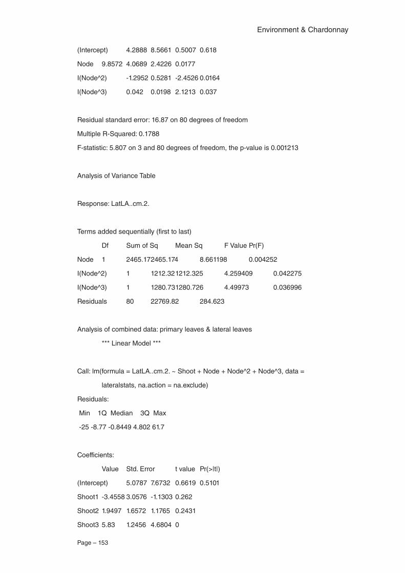
Page – 153
Environment & Chardonnay
(Intercept) 4.2888 8.5661 0.5007 0.618
Node 9.8572 4.0689 2.4226 0.0177
I(Node^2) -1.2952 0.5281 -2.4526 0.0164
I(Node^3) 0.042 0.0198 2.1213 0.037
Residual standard error: 16.87 on 80 degrees of freedom
Multiple R-Squared: 0.1788
F-statistic: 5.807 on 3 and 80 degrees of freedom, the p-value is 0.001213
Analysis of Variance Table
Response: LatLA..cm.2.
Terms added sequentially (first to last)
Df Sum of Sq Mean Sq F Value Pr(F)
Node 1 2465.17 2465.174 8.661198 0.004252
I(Node^2) 1 1212.32 1212.325 4.259409 0.042275
I(Node^3) 1 1280.73 1280.726 4.49973 0.036996
Residuals 80 22769.82 284.623
Analysis of combined data: primary leaves & lateral leaves
*** Linear Model ***
Call: lm(formula = LatLA..cm.2. ~ Shoot + Node + Node^2 + Node^3, data =
lateralstats, na.action = na.exclude)
Residuals:
Min 1Q Median 3Q Max
-25 -8.77 -0.8449 4.802 61.7
Coefficients:
Value Std. Error t value Pr(>|t|)
(Intercept) 5.0787 7.6732 0.6619 0.5101
Shoot1 -3.4558 3.0576 -1.1303 0.262
Shoot2 1.9497 1.6572 1.1765 0.2431
Shoot3 5.83 1.2456 4.6804 0
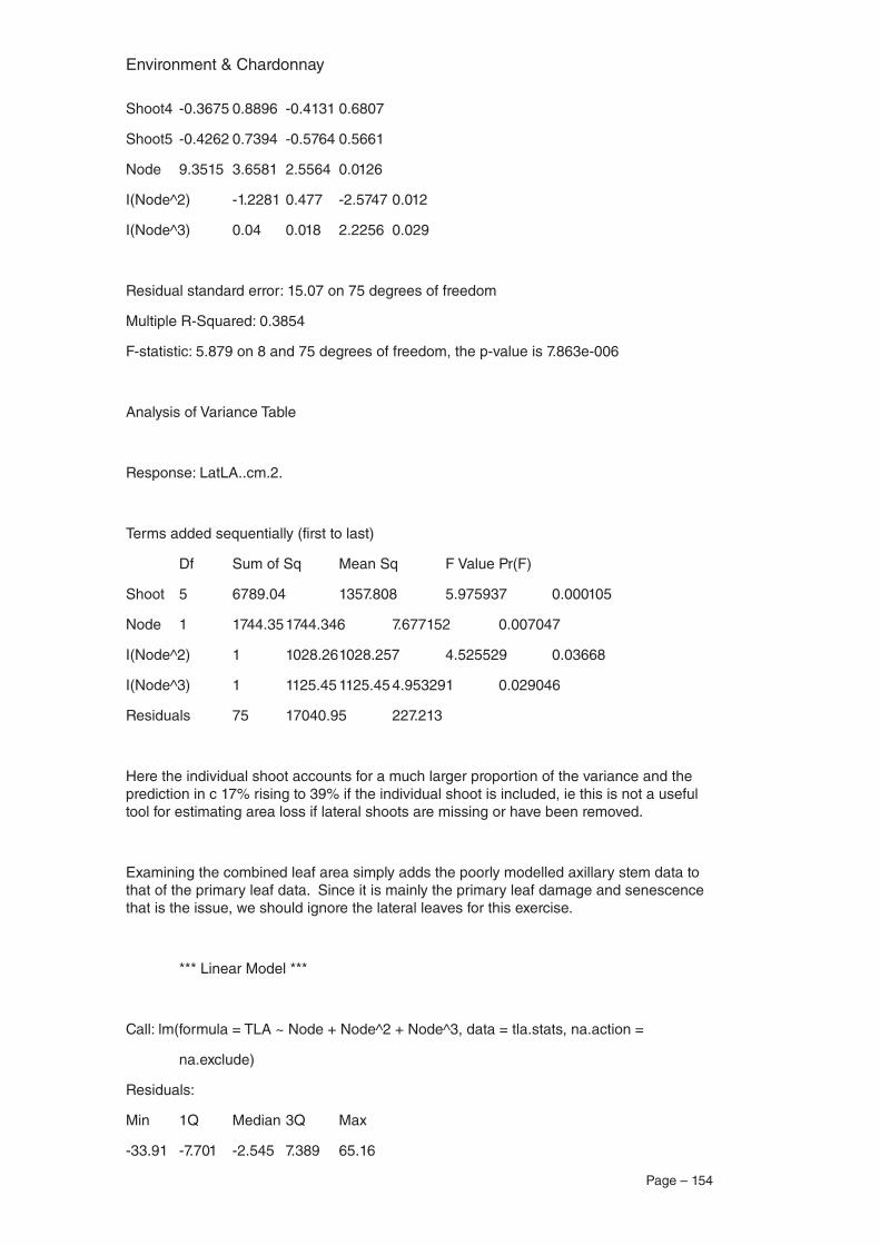
Environment & Chardonnay
Page – 154
Shoot4 -0.3675 0.8896 -0.4131 0.6807
Shoot5 -0.4262 0.7394 -0.5764 0.5661
Node 9.3515 3.6581 2.5564 0.0126
I(Node^2) -1.2281 0.477 -2.5747 0.012
I(Node^3) 0.04 0.018 2.2256 0.029
Residual standard error: 15.07 on 75 degrees of freedom
Multiple R-Squared: 0.3854
F-statistic: 5.879 on 8 and 75 degrees of freedom, the p-value is 7.863e-006
Analysis of Variance Table
Response: LatLA..cm.2.
Terms added sequentially (first to last)
Df Sum of Sq Mean Sq F Value Pr(F)
Shoot 5 6789.04 1357.808 5.975937 0.000105
Node 1 1744.35 1744.346 7.677152 0.007047
I(Node^2) 1 1028.26 1028.257 4.525529 0.03668
I(Node^3) 1 1125.45 1125.45 4.953291 0.029046
Residuals 75 17040.95 227.213
Here the individual shoot accounts for a much larger proportion of the variance and the prediction in c 17% rising to 39% if the individual shoot is included, ie this is not a useful tool for estimating area loss if lateral shoots are missing or have been removed.
Examining the combined leaf area simply adds the poorly modelled axillary stem data to that of the primary leaf data. Since it is mainly the primary leaf damage and senescence that is the issue, we should ignore the lateral leaves for this exercise.
*** Linear Model ***
Call: lm(formula = TLA ~ Node + Node^2 + Node^3, data = tla.stats, na.action =
na.exclude)
Residuals:
Min 1Q Median 3Q Max
-33.91 -7.701 -2.545 7.389 65.16
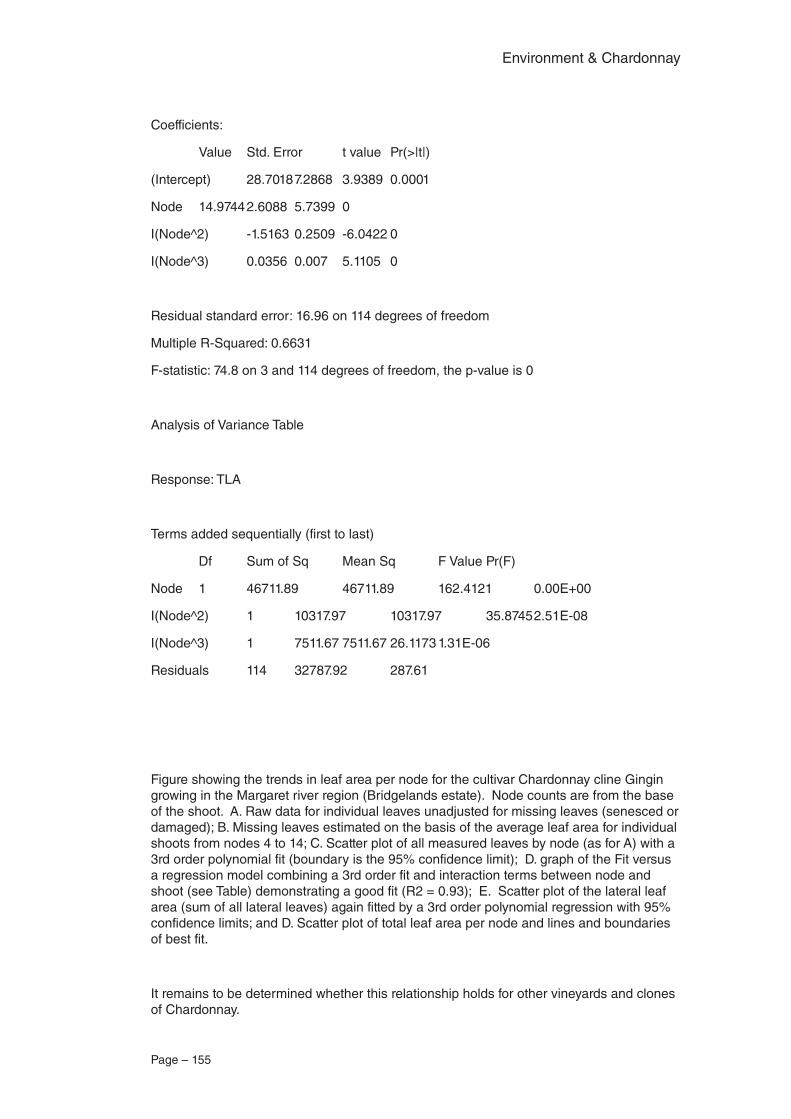
Page – 155
Environment & Chardonnay
Coefficients:
Value Std. Error t value Pr(>|t|)
(Intercept) 28.7018 7.2868 3.9389 0.0001
Node 14.9744 2.6088 5.7399 0
I(Node^2) -1.5163 0.2509 -6.0422 0
I(Node^3) 0.0356 0.007 5.1105 0
Residual standard error: 16.96 on 114 degrees of freedom
Multiple R-Squared: 0.6631
F-statistic: 74.8 on 3 and 114 degrees of freedom, the p-value is 0
Analysis of Variance Table
Response: TLA
Terms added sequentially (first to last)
Df Sum of Sq Mean Sq F Value Pr(F)
Node 1 46711.89 46711.89 162.4121 0.00E+00
I(Node^2) 1 10317.97 10317.97 35.8745 2.51E-08
I(Node^3) 1 7511.67 7511.67 26.1173 1.31E-06
Residuals 114 32787.92 287.61
Figure showing the trends in leaf area per node for the cultivar Chardonnay cline Gingin growing in the Margaret river region (Bridgelands estate). Node counts are from the base of the shoot. A. Raw data for individual leaves unadjusted for missing leaves (senesced or damaged); B. Missing leaves estimated on the basis of the average leaf area for individual shoots from nodes 4 to 14; C. Scatter plot of all measured leaves by node (as for A) with a 3rd order polynomial fit (boundary is the 95% confidence limit); D. graph of the Fit versus a regression model combining a 3rd order fit and interaction terms between node and shoot (see Table) demonstrating a good fit (R2 = 0.93); E. Scatter plot of the lateral leaf area (sum of all lateral leaves) again fitted by a 3rd order polynomial regression with 95% confidence limits; and D. Scatter plot of total leaf area per node and lines and boundaries of best fit.
It remains to be determined whether this relationship holds for other vineyards and clones of Chardonnay.
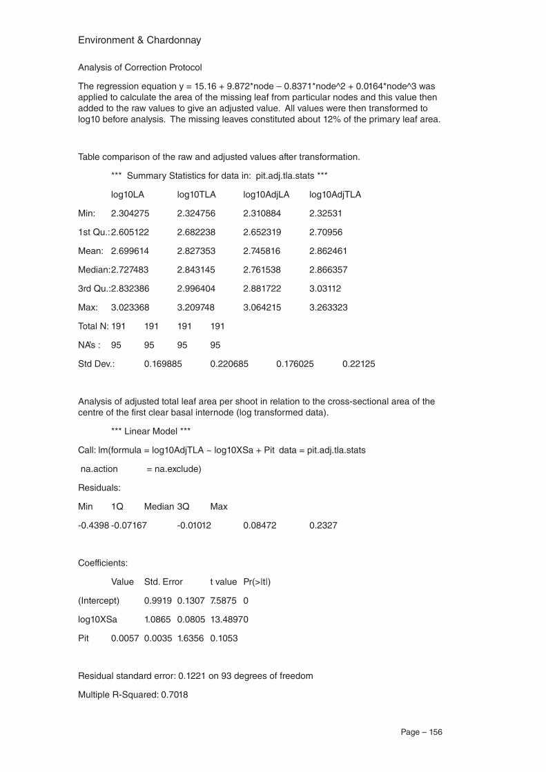
Environment & Chardonnay
Page – 156
Analysis of Correction Protocol
The regression equation y = 15.16 + 9.872*node – 0.8371*node^2 + 0.0164*node^3 was applied to calculate the area of the missing leaf from particular nodes and this value then added to the raw values to give an adjusted value. All values were then transformed to log10 before analysis. The missing leaves constituted about 12% of the primary leaf area.
Table comparison of the raw and adjusted values after transformation.
*** Summary Statistics for data in: pit.adj.tla.stats ***
log10LA log10TLA log10AdjLA log10AdjTLA
Min: 2.304275 2.324756 2.310884 2.32531
1st Qu.: 2.605122 2.682238 2.652319 2.70956
Mean: 2.699614 2.827353 2.745816 2.862461
Median: 2.727483 2.843145 2.761538 2.866357
3rd Qu.: 2.832386 2.996404 2.881722 3.03112
Max: 3.023368 3.209748 3.064215 3.263323
Total N: 191 191 191 191
NA’s : 95 95 95 95
Std Dev.: 0.169885 0.220685 0.176025 0.22125
Analysis of adjusted total leaf area per shoot in relation to the cross-sectional area of the centre of the first clear basal internode (log transformed data).
*** Linear Model ***
Call: lm(formula = log10AdjTLA ~ log10XSa + Pit data = pit.adj.tla.stats
na.action = na.exclude)
Residuals:
Min 1Q Median 3Q Max
-0.4398 -0.07167 -0.01012 0.08472 0.2327
Coefficients:
Value Std. Error t value Pr(>|t|)
(Intercept) 0.9919 0.1307 7.5875 0
log10XSa 1.0865 0.0805 13.4897 0
Pit 0.0057 0.0035 1.6356 0.1053
Residual standard error: 0.1221 on 93 degrees of freedom
Multiple R-Squared: 0.7018
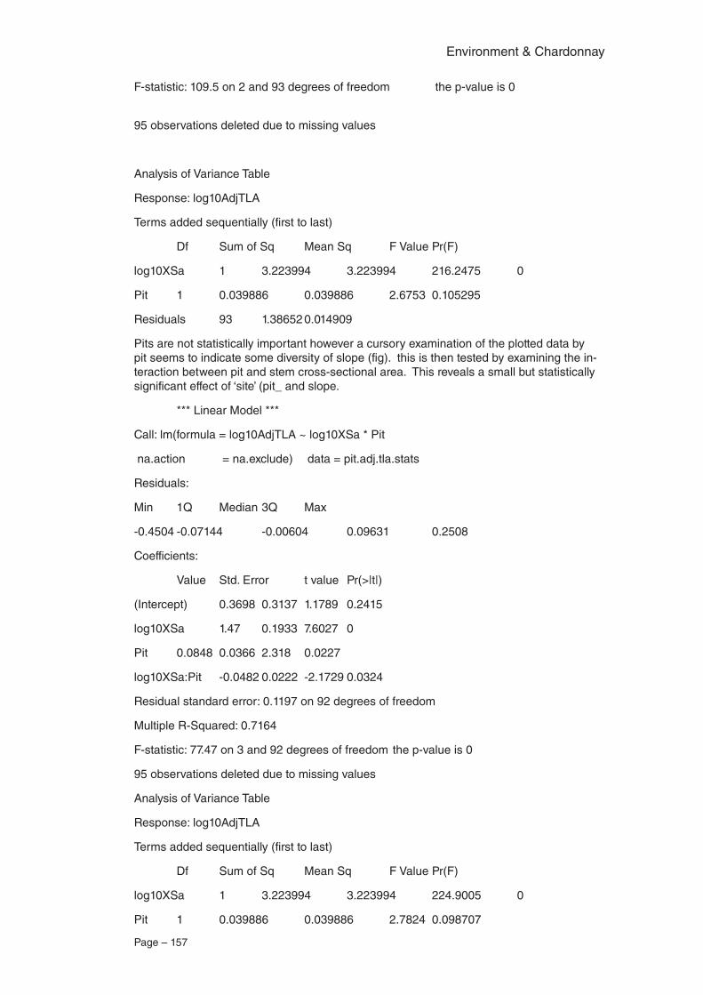
Page – 157
Environment & Chardonnay
F-statistic: 109.5 on 2 and 93 degrees of freedom the p-value is 0
95 observations deleted due to missing values
Analysis of Variance Table
Response: log10AdjTLA
Terms added sequentially (first to last)
Df Sum of Sq Mean Sq F Value Pr(F)
log10XSa 1 3.223994 3.223994 216.2475 0
Pit 1 0.039886 0.039886 2.6753 0.105295
Residuals 93 1.38652 0.014909
Pits are not statistically important however a cursory examination of the plotted data by pit seems to indicate some diversity of slope (fig). this is then tested by examining the in-teraction between pit and stem cross-sectional area. This reveals a small but statistically significant effect of ‘site’ (pit_ and slope.
*** Linear Model ***
Call: lm(formula = log10AdjTLA ~ log10XSa * Pit
na.action = na.exclude) data = pit.adj.tla.stats
Residuals:
Min 1Q Median 3Q Max
-0.4504 -0.07144 -0.00604 0.09631 0.2508
Coefficients:
Value Std. Error t value Pr(>|t|)
(Intercept) 0.3698 0.3137 1.1789 0.2415
log10XSa 1.47 0.1933 7.6027 0
Pit 0.0848 0.0366 2.318 0.0227
log10XSa:Pit -0.0482 0.0222 -2.1729 0.0324
Residual standard error: 0.1197 on 92 degrees of freedom
Multiple R-Squared: 0.7164
F-statistic: 77.47 on 3 and 92 degrees of freedom the p-value is 0
95 observations deleted due to missing values
Analysis of Variance Table
Response: log10AdjTLA
Terms added sequentially (first to last)
Df Sum of Sq Mean Sq F Value Pr(F)
log10XSa 1 3.223994 3.223994 224.9005 0
Pit 1 0.039886 0.039886 2.7824 0.098707
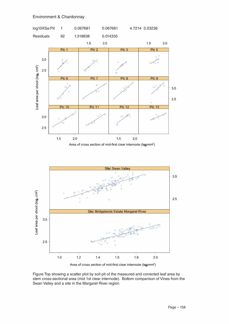
Environment & Chardonnay
Page – 158
log10XSa:Pit 1 0.067681 0.067681 4.7214 0.03236
Residuals 92 1.318838 0.014335
Figure Top showing a scatter plot by soil pit of the measured and corrected leaf area by stem cross-sectional area (mid 1st clear internode). Bottom comparison of Vines from the Swan Valley and a site in the Margaret River region
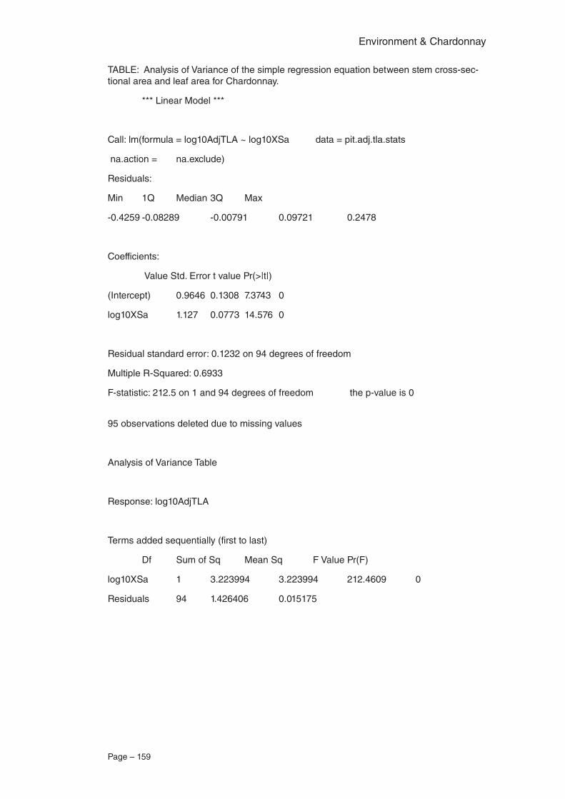
Page – 159
Environment & Chardonnay
TABLE: Analysis of Variance of the simple regression equation between stem cross-sec-tional area and leaf area for Chardonnay.
*** Linear Model ***
Call: lm(formula = log10AdjTLA ~ log10XSa data = pit.adj.tla.stats
na.action = na.exclude)
Residuals:
Min 1Q Median 3Q Max
-0.4259 -0.08289 -0.00791 0.09721 0.2478
Coefficients:
Value Std. Error t value Pr(>|t|)
(Intercept) 0.9646 0.1308 7.3743 0
log10XSa 1.127 0.0773 14.576 0
Residual standard error: 0.1232 on 94 degrees of freedom
Multiple R-Squared: 0.6933
F-statistic: 212.5 on 1 and 94 degrees of freedom the p-value is 0
95 observations deleted due to missing values
Analysis of Variance Table
Response: log10AdjTLA
Terms added sequentially (first to last)
Df Sum of Sq Mean Sq F Value Pr(F)
log10XSa 1 3.223994 3.223994 212.4609 0
Residuals 94 1.426406 0.015175
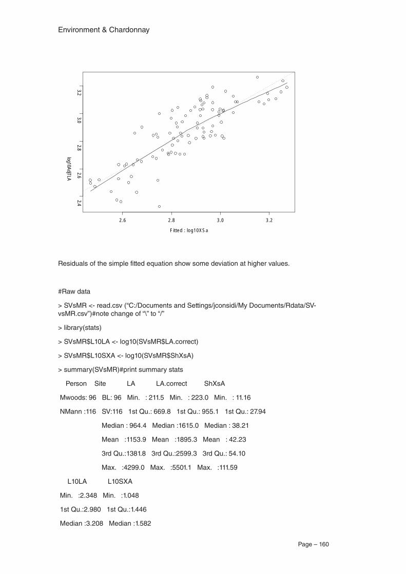
Environment & Chardonnay
Page – 160
F itted : log10XS a
log10AdjTLA
2 .6 2 .8 3 .0 3 .2
2.42.6
2.83.0
3.2
Residuals of the simple fitted equation show some deviation at higher values.
#Raw data
> SVsMR <- read.csv (“C:/Documents and Settings/jconsidi/My Documents/Rdata/SV-vsMR.csv”)#note change of “\” to “/”
> library(stats)
> SVsMR$L10LA <- log10(SVsMR$LA.correct)
> SVsMR$L10SXA <- log10(SVsMR$ShXsA)
> summary(SVsMR)#print summary stats
Person Site LA LA.correct ShXsA
Mwoods: 96 BL: 96 Min. : 211.5 Min. : 223.0 Min. : 11.16
NMann :116 SV:116 1st Qu.: 669.8 1st Qu.: 955.1 1st Qu.: 27.94
Median : 964.4 Median :1615.0 Median : 38.21
Mean :1153.9 Mean :1895.3 Mean : 42.23
3rd Qu.:1381.8 3rd Qu.:2599.3 3rd Qu.: 54.10
Max. :4299.0 Max. :5501.1 Max. :111.59
L10LA L10SXA
Min. :2.348 Min. :1.048
1st Qu.:2.980 1st Qu.:1.446
Median :3.208 Median :1.582
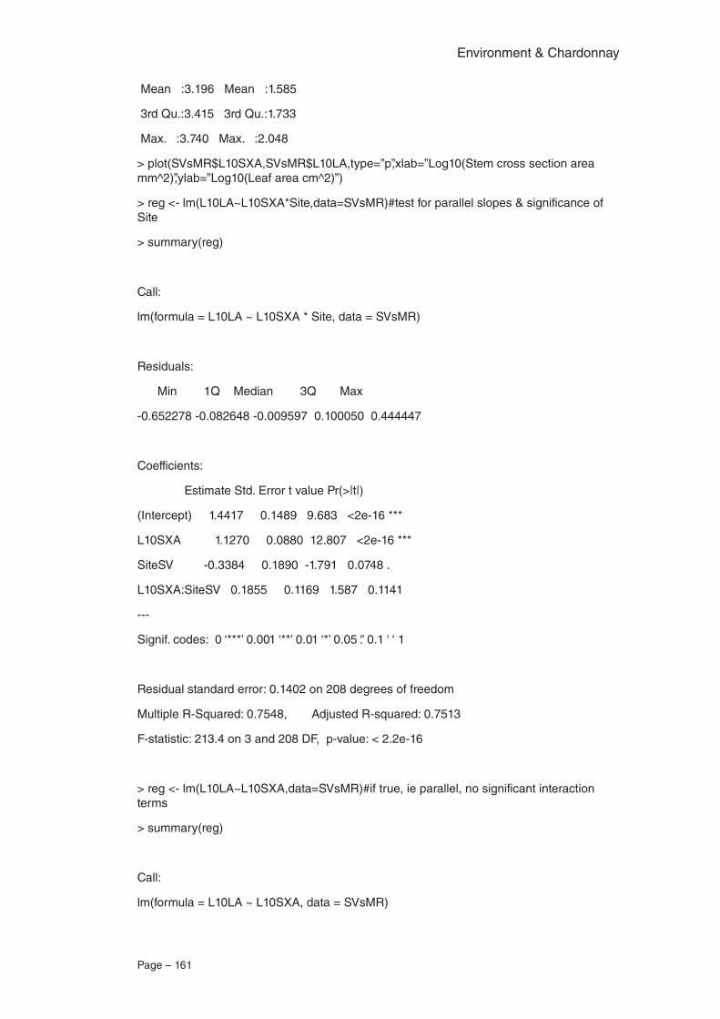
Page – 161
Environment & Chardonnay
Mean :3.196 Mean :1.585
3rd Qu.:3.415 3rd Qu.:1.733
Max. :3.740 Max. :2.048
> plot(SVsMR$L10SXA,SVsMR$L10LA,type=”p”,xlab=”Log10(Stem cross section area mm^2)”,ylab=”Log10(Leaf area cm^2)”)
> reg <- lm(L10LA~L10SXA*Site,data=SVsMR)#test for parallel slopes & significance of Site
> summary(reg)
Call:
lm(formula = L10LA ~ L10SXA * Site, data = SVsMR)
Residuals:
Min 1Q Median 3Q Max
-0.652278 -0.082648 -0.009597 0.100050 0.444447
Coefficients:
Estimate Std. Error t value Pr(>|t|)
(Intercept) 1.4417 0.1489 9.683 <2e-16 ***
L10SXA 1.1270 0.0880 12.807 <2e-16 ***
SiteSV -0.3384 0.1890 -1.791 0.0748 .
L10SXA:SiteSV 0.1855 0.1169 1.587 0.1141
---
Signif. codes: 0 ‘***’ 0.001 ‘**’ 0.01 ‘*’ 0.05 ‘.’ 0.1 ‘ ‘ 1
Residual standard error: 0.1402 on 208 degrees of freedom
Multiple R-Squared: 0.7548, Adjusted R-squared: 0.7513
F-statistic: 213.4 on 3 and 208 DF, p-value: < 2.2e-16
> reg <- lm(L10LA~L10SXA,data=SVsMR)#if true, ie parallel, no significant interaction terms
> summary(reg)
Call:
lm(formula = L10LA ~ L10SXA, data = SVsMR)
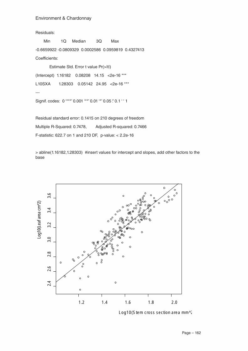
Environment & Chardonnay
Page – 162
Residuals:
Min 1Q Median 3Q Max
-0.6659922 -0.0809329 0.0002586 0.0959819 0.4327413
Coefficients:
Estimate Std. Error t value Pr(>|t|)
(Intercept) 1.16182 0.08208 14.15 <2e-16 ***
L10SXA 1.28303 0.05142 24.95 <2e-16 ***
---
Signif. codes: 0 ‘***’ 0.001 ‘**’ 0.01 ‘*’ 0.05 ‘.’ 0.1 ‘ ‘ 1
Residual standard error: 0.1415 on 210 degrees of freedom
Multiple R-Squared: 0.7478, Adjusted R-squared: 0.7466
F-statistic: 622.7 on 1 and 210 DF, p-value: < 2.2e-16
> abline(1.16182,1.28303) #insert values for intercept and slopes, add other factors to the base
1 .2 1 .4 1 .6 1 .8 2 .0
2.42.6
2.83.0
3.23.4
3.6
L og10(S tem cross section a rea m m ^2)
Log1
0(Le
af ar
ea cm
^2)
Page – 163
Environment & Chardonnay
Theses supported by this and a pilot project
PhDWisdom , J. (200x). Managing the vine for precise (predictable) outcomes: observing, understanding
and managing heterogeneity in the vineyard (suspended for family reasons, anticipated completion Dec 2009).
Fourth Year ProjectsHipper, L. (2005) The Importance of Wine Aroma: Quantitative Assessment of Amino Acid Uptake by
Saccharomyces in Wine.
Gazey, C. (2006). The Influence of Calcium and Magnesium on Fermentation Kinetics and Flocculation in a White Wine Fermentation
Wood, M. (2006) Towards Objective Management Practices in Viticulture: Water status and nitrogen metabolism in Chardonnay grapevines.
Miyata, D. (2005) Modelling scattering and absorption behaviours of a bunch of grapes.
Maley, K. (2006). Hexose transporter gene expression during stuck and sluggish wine fermentations. Perth: UWA; 2006.
Isaac, A. (2007). Hexose Transporter Gene Expression During Stuck and Sluggish Wine Fermentations
Clarke, N. (2003). Leaf Area to Fruit Weight Ratio of Chardonnay (Vitis vinifera L.): Role in Maximising Fruit Quality for Premium Wine Production.
Pearce, S. (2003) Impact of Climate on the Composition of Chardonnay Fruit.
Bennett, J. (2003) Exploration of variation in Vitis vinifera (L. cv. Cabernet Sauvignon) fruit maturity: An application of optical remote sensing to maturity sampling.
Robinson, AL. (2003) Quantitative Assessment of Grape Quality Influence of Site and Clone on cv. Chardonnay
Copies of all these are available on request.

Environment & Chardonnay
Page – 164


