Embed Size (px)
Citation preview
Validation of CFD Predictions of Urban Wind
By
Riley Willis
A thesis submitted to Victoria University of Wellington
in fulfilment of the requirements for the degree of Master of Building Science
Victoria University of Wellington 2017
Developing a Methodology


i
Abstract “Good mental health in a fluid or CFD modeller is always indicated by the presence of a suspicious nature, cynicism and a ‘show me’ attitude. These are not necessarily the best traits for a life mate or a best friend, but they are essential if the integrity of the modelling process is to be maintained”
(Meroney, 2004)
Over the past 50 years, Computational Fluid Dynamics (CFD) computer simulation programs have offered a new method of calculating the wind comfort and safety data for use in pedestrian wind studies. CFD models claim to have some important advantages over wind tunnels; which remain the most common method of wind calculation. While wind tunnels provide measurements of selected points, CFD simulations provide whole-flow field data for the entire area under investigation (Blocken, 2014; Blocken, Stathopoulos, & van Beeck, 2016). Similarly, wind tunnel measurements must consider the similarity requirements involved with testing a model at small scale, while CFD simulations can avoid this as they are conducted at full scale (Ramponi & Blocken, 2012a).
However, CFD simulations can also often be misleading; and they should only be trusted once they can be proven to be accurate. To appease the requirements for this cynical view- referenced in the above quote- proper verification and validation of a model is imperative.
This thesis investigated and tested the current best practice guidelines around CFD model validation, using existing wind tunnel measurements of generic urban arrays. The goal of the research was to determine whether the existing data and guidance around the validation process was sufficient for a consultant user to trust that a CFD model they created was sufficiently accurate to base design decisions from.
The CFD code Autodesk CFD was used to simulate two configurations first tested as wind tunnel models by the Architectural Institute of Japan, and Opus labs in Wellington. The Wellington City Council wind speed criteria were used to determine whether the CFD simulations met the required accuracy criteria for council consent.
Results from the study found that the CFD models could not meet the accuracy criteria. It concluded that while the validation process provided sufficient guidance, there is a lack of available data which is relevant to CFD validation for urban flows.
It was recommended that at least one improved dataset was required, to build a system by which a consultant can identify what the requirements of a CFD model are to provide accurate CFD analysis of the site under investigation. To accommodate the range of sites likely to be present in urban wind studies, it was recommended that the new dataset provided data for a variety of wind flows likely to be found in cities.

ii

iii
Acknowledgements Firstly and foremost, I would like to express my deep gratitude to my supervisor, Dr. Michael Donn, for his tireless guidance, suggestions and support over the course of this thesis.
Thank you to Paul Carpenter from Opus Consultants, who provided the original wind tunnel data for this study. Your support and guidance were immensely valuable over the thesis. Thank you also to Professor Koji Sakai. Your advice and support in understanding the CFD simulation process, as well as some translation of the Japanese texts was greatly appreciated.
I would also like to extend my thanks to the School of Architecture’s IT Services team: Stewart Milne, Peter Ramutenas, and Eric Camplin. This research would not have been possible without their work installing software, re-installing software, and troubleshooting issues.
Thank you to my fellow students Cameron Smith, Louise Ing, Tanvi Bhagwat, Charles Thaxter, Julia Thompson, Jamie Sullivan, Elzine Braasch, and Ethan Duff for taking notes in the numerous meetings, bouncing ideas off each other and for your most helpful feedback.
Thank you to my family for your interest in my research, for proof-reading and providing feedback, and for your support throughout my studies.
Finally, thank you to all of my friends not mentioned above, and especially to the amazing Mere Rawalai, for your patience, care and support throughout the year.
iv
Contents 1. CFD Predictions of Urban Wind ......................................................................... 1
Why is Wellington a suitable test city for CFD validation? ............................. 3
The City of London is also investigating alternatives to the current testing process ................................................................................................................. 5
CFD could help consultants communicate with designers and planners to properly implement design strategies ................................................................... 6
Questions to address .................................................................................. 7
Goals .......................................................................................................... 7
2. Validation of CFD Predictions of Urban Wind ..................................................... 8
The current state of CFD validation for urban wind prediction ...................... 8
The types of validation configuration ......................................................... 10
The comparison table: a guide ....................................................................11
Findings from the comparison table .......................................................... 21
2.4.1 Access to data is a major limitation ..................................................... 21
2.4.2 Very few studies consider justifying how the model is “representative” of a real city to be important................................................................................ 21
2.4.3 Uniform height blocks are not representative of most real-world urban environments. ................................................................................................. 23
2.4.4 The size of the array is an important factor. ........................................ 24
What is the significance of these findings? ................................................. 25
Which configurations are viable CFD validation sets? ................................. 26
2.6.1 Configurations 14 & 16: The AIJ dataset .............................................. 26
2.6.2 Configuration 4: The Wellington “Standard City” set ........................... 27
CFD for urban wind flows .......................................................................... 28
2.7.1 Overview and discretisation methods ................................................. 28
2.7.2 Meshing ............................................................................................. 30
2.7.3 Modelling Turbulence and the Simulation Process .............................. 32
2.7.4 Verification & Validation Best Practice Guidelines ............................... 35
Wind tunnel and Small Scale modelling ...................................................... 37
2.8.1 Wind Tunnel Measurement techniques ............................................... 38
2.8.2 How Ohms law is used to estimate wind speeds .................................. 39
v
2.8.3 Split film anemometry ........................................................................ 39
2.8.4 Hot film anemometry ......................................................................... 39
2.8.5 Information required for CFD validation .............................................. 40
3. The CFD Validation Process ............................................................................. 41
The best validation method is through comparison to wind tunnel measurements .................................................................................................... 42
3.1.1 The BESTEST definition of validation .................................................. 42
3.1.2 What is the BESTEST validation test for CFD? ..................................... 43
The first step in a CFD validation process should be a simple test of the CFD
code using a single block configuration. ............................................................... 45
Both configurations identified in the literature should be used as validation datasets.............................................................................................................. 46
The AIJ wind tunnel tests omit potentially important data points ............... 48
3.4.1 Wind speed measurement points ........................................................ 48
3.4.2 Wind profile comparison .................................................................... 49
How trustworthy are the wind tunnels? ..................................................... 50
Autodesk CFD is the Most Appropriate code for the validation ................... 51
Available codes ......................................................................................... 53
3.7.1 Simulation CFD .................................................................................. 53
3.7.2 UrbaWind .......................................................................................... 55
3.7.3 StarCCM+ .......................................................................................... 57
3.7.4 Code selection ................................................................................... 58
An existing CFD validation process can be used to test model accuracy ...... 59
3.8.1 Computational domain and initial conditions ...................................... 60
3.8.2 Mesh sensitivity analysis ..................................................................... 61
3.8.3 A description of the various turbulence models ................................... 61
3.8.4 Data Analysis ..................................................................................... 62
Existing wind speed criteria can be used to define accuracy ........................ 64
3.9.1 The Effective gust speed accuracy criteria ........................................... 66
3.9.2 How do effective gust speeds fit with WCC compliance criteria? .......... 68
4. Determining Appropriate Parameters for the CFD Validation Study .................. 71
A test using the AIJ simple block ................................................................. 71
vi
4.1.1 CFD simulation setup ......................................................................... 72
4.1.2 Results of the simple block test ........................................................... 75
Testing the AIJ city dataset ....................................................................... 78
4.2.1 Simulation set-up ............................................................................... 78
4.2.2 Grouping the measurement points helps to identify and compare the flow features ................................................................................................... 82
4.2.3 Comparing the measurement points was a source of difficulty with the Autodesk CFD code. ........................................................................................... 85
4.2.4 Mesh resolution has a notable impact on the results ............................ 86
4.2.5 Linking the graphed results to observed wind flow features ................. 89
4.2.6 Changing the turbulence model has a small effect on the simulation ... 92
Extra simulations were carried out to test the validation process ................ 94
4.3.1 Could simulating a model at small scale improve accuracy? ................. 94
4.3.2 Does changing the turbulent intensity factor have a significant effect? 96
Final validation using accuracy criteria: is the CFD model trustworthy? ..... 100
Conclusions from the comparison graphs ................................................ 102
4.5.1 The CFD models were not sufficiently accurate to be used ................ 102
4.5.1 The validation process was a successful method of determining CFD trustworthiness ............................................................................................. 102
Testing the Standard City dataset ............................................................ 103
4.6.1 Simulation set-up .............................................................................. 103
4.6.2 Mesh resolution significantly impacts the results ............................... 108
4.6.3 Changing the turbulence model has a small bur noticeable effect on the results 110
4.6.4 Is a bigger array necessarily better? ................................................... 112
Does the Standard City configuration give different validation results? ..... 116
4.7.1 Results in the windward direction ...................................................... 116
4.7.2 Diagonal Wind Direction Analysis ...................................................... 117
Conclusions from the comparison graphs ................................................. 119
4.8.1 The CFD models created for the test did not meet the accuracy criteria 119
4.8.2 There were some inconsistencies in the flow features described by the wind tunnel datasets ......................................................................................... 120
vii
4.8.3 The channelling effect observed in the smaller array is not necessarily a drawback ...................................................................................................... 120
Summary ................................................................................................. 121
5. Conclusions from the CFD Validation Study ................................................... 122
What needs to be included in a validation dataset? .................................. 122
5.1.1 The 3D geometry of the dataset is an important consideration .............. 123
5.1.2 Comments on the suitability of the Standard City and AIJ configurations as a CFD validation suite. .......................................................................................125
What do the results of the CFD validation test mean? .............................. 126
5.1.3 Choice of CFD code is an important factor ............................................ 126
5.1.4 Consultants should spend the largest amount of time designing the computational mesh. ......................................................................................... 127
An appropriate configuration for CFD validation of Urban CFD flows should focus on modelling flow features, not specific geometries. .................................. 127
Presentation and availability of data are important factors ....................... 128
Future incorporation into standards......................................................... 129
Appendix I: Results of CFD simulations ........................................................... 139
AIJ 2:1:1 Block ................................................................................................ 139
X-direction Flows ........................................................................................... 139
Y-direction flows ........................................................................................... 140
Z-Direction Flows ........................................................................................... 141
AIJ Tall Tower in a Uniform City model: ......................................................... 142
Windward Mesh Sensitivity Analysis .............................................................. 142
Windward tests Using SST k-w and RNG turbulence models ...........................145
Windward Turbulent Intensity Effects ............................................................ 146
Windward flow modelled at wind tunnel scale ................................................. 147
Diagonal Wind flow Mesh Sensitivity Analysis ................................................ 148
Diagonal flow using SST k-w and RNG turbulence models ............................... 151
Diagonal flow turbulent intensity effects ........................................................152
Diagonal flow modelled at wind tunnel scale ................................................... 153
Standard City Configuration ...........................................................................154
Windward flow Mesh Sensitivity Analysis ........................................................154
Windward tests Using SST k-w and RNG turbulence models ........................... 157
viii
Windward Turbulent Intensity Effects .............................................................158
Windward effects simulating a large array ......................................................158
Diagonal Wind flow Mesh Sensitivity Analysis ................................................ 159
Diagonal flow SST k-w and RNG turbulence models ....................................... 162
Diagonal flow turbulent intensity effects ........................................................ 163
Diagonal flow simulating a large array ............................................................ 163
Appendix II: CFD validation using Lawson Criteria .......................................... 165
ix
Figures Figure 1: Pedestrian Discomfort caused by the local wind climate .............................. 1
Figure 2: Wind funnelling through Cook Straight. Adapted from (Virtual Terrain Project, n.d.) ............................................................................................................. 3
Figure 3: Table showing the make-up of urban streets in Eindhoven, ND. Source: (Ramponi et al., 2015) .................................................. Error! Bookmark not defined.
Figure 4: Skimming flow between uniform height blocks. Adapted from (Millward-Hopkins et al., 2011)................................................................................................ 24
Figure 5: Venn Diagram of assessed generic forms (author’s image) ......................... 25
Figure 6: Illustration of the mesh resolution concept, using the approximation of a curve as an example (author’s image) ...................................................................... 30
Figure 7: Structured grid (left) vs unstructured mesh (right) ......................................31
Figure 8: CFD Convergence plot (author's image) .................................................... 33
Figure 9: LES (Left) vs RANS (right) simulation of air mixing. Source: (Durrani et al., 2015) ...................................................................................................................... 34
Figure 10: An example of the strong visual nature of CFD, showing the increase of wind speed with height, and its interaction with a tall tower (Author’s image) .......... 35
Figure 11: Axonometric view of the 2:1:1 block configuraton .................................... 45
Figure 12: Simple Block Measurement points (Architectural Institute of Japan, 2016). .............................................................................................................................. 46
Figure 13: AIJ measurement locations ..................................................................... 48
Figure 14: Standard City measurement locations ..................................................... 49
Figure 15: AIJ vs Deaves & Harris inlet profiles ......................................................... 50
Figure 16: CFD validation process outlined by Blocken, Janssen, & van Hoof (2012) .. 59
Figure 17: Autodesk external flow computational domain (Autodesk, n.d.-e) ............ 60
Figure 18: Example line comparison graph ............................................................... 63
Figure 19: Comparison scatter plot for CFD vs wind tunnel ....................................... 63
Figure 20: Example of effective gust speed plots ..................................................... 69
Figure 21: Single Block computational domain ........................................................ 72
Figure 22: Single Block Inlet Profile ......................................................................... 72
Figure 23: Measurement point overlaid with CFD analysis results ............................. 75
Figure 24: x-axis comparison line graph .................................................................... 77
Figure 25: y-axis comparison line graph .................................................................... 77
x
Figure 26: x-axis comparison line graph .................................................................... 77
Figure 27: AIJ Configuration Lengthwise Computational Domain ............................. 78
Figure 28: AIJ Configuration Widthways Computational Domain ............................. 79
Figure 29: AIJ 0° Comparison line graph (top) and scatter plots for 0.2, 0.25 and 0.15 mesh resolutions (bottom) ...................................................................................... 88
Figure 30: AIJ 45° Comparison line graph (top) and scatter plots for 0.2, 0.25 and 0.15 mesh resolutions (bottom) ...................................................................................... 88
Figure 31: schematic showing Corner effect (1) and Downdraught effect (2). Adapted from (Gandemer, 1975; Pendwarden & Wise, 1975). ................................................. 89
Figure 32: x- direction comparison of CFD vs Wind Tunnel between points 25-42 ..... 90
Figure 33: y- direction comparison of CFD vs Wind Tunnel between points 25-42 ...... 90
Figure 34: z- direction comparison of CFD vs Wind Tunnel between points 25-42 ..... 90
Figure 35: CFD vector diagram of the downdraught effect ....................................... 91
Figure 36: AIJ 0°-line graph (top) and scatter plots (bottom) comparing k-e, SST k-w, and RNG turbulence models ................................................................................... 93
Figure 37: AIJ 45°-line graph (top) and scatter plots (bottom) comparing k-e, SST k-w, and RNG turbulence models ................................................................................... 93
Figure 38: Longitudinal comparison graph, scaled down model ................................ 95
Figure 39:Diagonal comparison graph, scaled down model ...................................... 96
Figure 40: AIJ Turbulent Intensity Profile ................................................................. 97
Figure 41: Effect of changing turbulent intensity: AIJ 0°-line graph (top) and scatter plots (bottom) ........................................................................................................ 98
Figure 42: Effect of changing turbulent intensity: AIJ 45°-line graph (top) and scatter plots (bottom) ........................................................................................................ 98
Figure 43: Windward direction comparative plots of CFD vs wind tunnel measurements using effective gust speed ............................................................. 100
Figure 44: Diagonal wind direction comparative plots of CFD vs wind tunnel measurements using effective gust speed .............................................................. 101
Figure 45: Standard City Configuration Lengthwise Computational Domain ........... 103
Figure 46: Standard City Configuration Widthways Computational Domain ............ 103
Figure 47: Standard City 0°-line graph (top) and scatter plots comparing 0.2, 0.25 and 0.15 mesh resolutions (bottom) ............................................................................. 109
Figure 48: Standard City 45°-line graph (top) and scatter plots comparing 0.2, 0.25 and 0.15 mesh resolutions (bottom) ............................................................................. 109
xi
Figure 49: 0°-line graph (top) and scatter plots (bottom) comparing k-e, SST k-w, and RNG turbulence models ......................................................................................... 111
Figure 50: 45°-line graph (top) and scatter plots (bottom) comparing k-e, SST k-w, and RNG turbulence models ......................................................................................... 111
Figure 51: Larger Standard City Configuration design ............................................. 113
Figure 52: Standard City 0°-line graph (top) and scatter plots (bottom) comparing 5x5 and 10 x 9 arrays .................................................................................................... 115
Figure 53: Standard City 45°-line graph (top) and scatter plots (bottom) comparing 5x5 and 10 x 9 arrays .................................................................................................... 115
Figure 54: Windward direction comparative plots of CFD vs wind tunnel measurements using effective gust speed .............................................................. 117
Figure 55: Diagonal direction comparative plots of CFD vs wind tunnel measurements using effective gust speed ...................................................................................... 118
Figure 56: Wellington city high-rise building layout. Adapted from (Google Maps, 2016) .................................................................................................................... 124
Figure 57: Wind effects around buildings. Adapted from (Gandemer, 1975). ........... 128
Figure 58: Lawson Criteria Applied to Standard City wind tunnel measurements .... 168
Figure 59: Windward direction comparative plots of CFD vs wind tunnel measurements using mean wind speed ................................................................. 169
Figure 60: Diagonal wind direction comparative plots of CFD vs wind tunnel measurements using mean wind speed .................................................................. 170
Figure 61: Windward direction comparative plots of CFD vs wind tunnel measurements using mean wind speed .................................................................. 171
Figure 62: Diagonal direction comparative plots of CFD vs wind tunnel measurements using mean wind speed .......................................................................................... 172
xii
Tables Table 1: Average wind speeds for cities around the world. Adapted from (Ligget & Milne, n.d.) .............................................................................................................................. 4
Table 2: Generic vs Urban arrays. Adapted from (Blocken et al., 2016). ........................... 11
Table 3: Comparison table of 29 generic urban configurations used in literature ............. 14
Table 4: Representative city justifications from the table .............................................. 22
Table 5: Discretisation method comparison. Adapted from (Zapka, 2014) ...................... 28
Table 6: Numerical and Physical Errors in CFD (Adapted from (Franke et al., 2007)) ....... 36
Table 7: Comparison of validation types........................................................................ 44
Table 8: AIJ and Standard City configuration comparison .............................................. 46
Table 9: Performance of Autodesk Simulation CFD against the specified CFD code criteria ................................................................................................................................... 53
Table 10: Performance of Meteodyn’s UrbaWind against the specified CFD code criteria 55
Table 11:Performance of CD Adapco's StarCCM+ against the specified CFD code criteria 57
Table 12: Turbulence model comparison....................................................................... 62
Table 13: WCC gust speed requirements. Adapted from (Carpenter, 2002) .................... 68
Table 14: Detailed effective gust speed categories. Adapted from (Carpenter, 2002) ..... 68
Table 15: Mesh resolution iterations for sensitivity analysis using simple block configuration ............................................................................................................... 74
Table 16: AIJ Tall Tower Boundary Conditions ............................................................... 79
Table 17:Mesh resolution iterations for sensitivity analysis of AIJ Tall tower in a city configuration ............................................................................................................... 80
Table 18: Labelling system for identifying flow groupings in line graphs ......................... 83
Table 19: AIJ flow identification groupings and measuring points for both flow directions ................................................................................................................................... 84
Table 20: How a small variation to the input can invalidate the measurement points ...... 85
Table 21: Standard City Boundary Conditions ............................................................. 104
Table 22: Mesh resolution iterations for sensitivity analysis of Standard City configuration ................................................................................................................................. 104
Table 23: Labelling system for identifying flow groupings in line graphs ....................... 106
Table 24: Standard City flow identification groupings and measuring points for both flow directions ................................................................................................................... 107
Table 25: Lawson Criteria, adapted from (Shilston, 2015). ........................................... 166
1
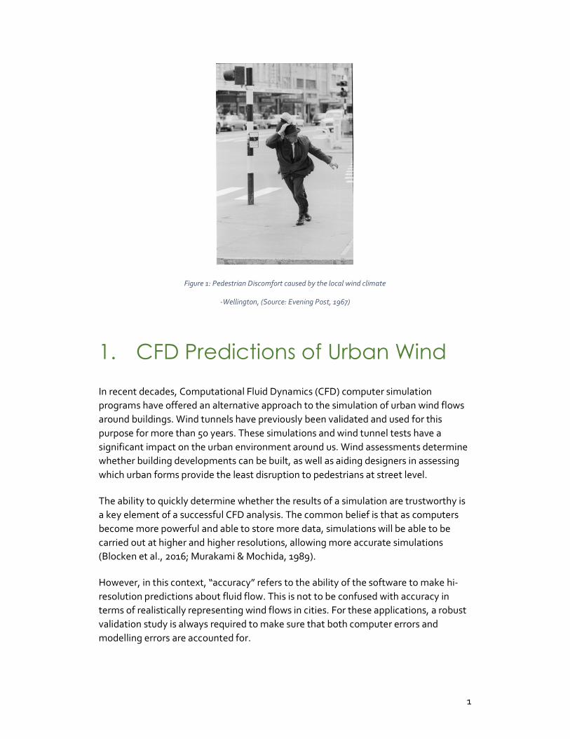
Figure 1: Pedestrian Discomfort caused by the local wind climate
-Wellington, (Source: Evening Post, 1967)
1. CFD Predictions of Urban Wind
In recent decades, Computational Fluid Dynamics (CFD) computer simulation programs have offered an alternative approach to the simulation of urban wind flows around buildings. Wind tunnels have previously been validated and used for this purpose for more than 50 years. These simulations and wind tunnel tests have a significant impact on the urban environment around us. Wind assessments determine whether building developments can be built, as well as aiding designers in assessing which urban forms provide the least disruption to pedestrians at street level.
The ability to quickly determine whether the results of a simulation are trustworthy is a key element of a successful CFD analysis. The common belief is that as computers become more powerful and able to store more data, simulations will be able to be carried out at higher and higher resolutions, allowing more accurate simulations (Blocken et al., 2016; Murakami & Mochida, 1989).
However, in this context, “accuracy” refers to the ability of the software to make hi-resolution predictions about fluid flow. This is not to be confused with accuracy in terms of realistically representing wind flows in cities. For these applications, a robust validation study is always required to make sure that both computer errors and modelling errors are accounted for.

Validation of CFD Predictions of Urban Wind
2
This thesis examines the means by which consultant users of CFD investigating wind effects on pedestrians might demonstrate that the computer program itself, and their use of it, can be trusted. To do this in a meaningful way, a standard process for validation of CFD models is required.
However, no definitive method currently exists for consultants to show whether their CFD models are trustworthy. This is in part due to a lack of robust datasets to validate the CFD models against, and due to a lack of a standardised CFD validation process. Fortunately, due to the wealth of wind tunnel tests which have been carried out in past research, several datasets exist which may be suitable for CFD validation. This research proposes to firstly identify and secondly test the suitability of potential data sets for CFD validation. As the investigation centres around predicting the effects of wind in cities, the notoriously windy Wellington city has been chosen as the setting for this investigation.
Validation of CFD Predictions of Urban Wind
3
Why is Wellington a suitable test city for CFD validation?
- 68m/s: The highest gust of wind ever recorded in Wellington. - 8m/s: Average wind speed at Wellington Airport. - 233 days: Number of days that winds exceeded “gale force” speeds in
Wellington’s windiest year
(Fitzsimons, 2011).
To model wind in a city, you need a city that has wind. When looked at on an average wind speed basis, Wellington is renowned as one of the windiest cities in the world. The reason for the wind is a combination of location and geography. New Zealand’s location in the “roaring forties”- a belt of strong winds in the southern hemisphere between latitudes of 40 to 49 degrees- is one reason why the country as a whole receives strong winds (Turner & Revell, 2011).
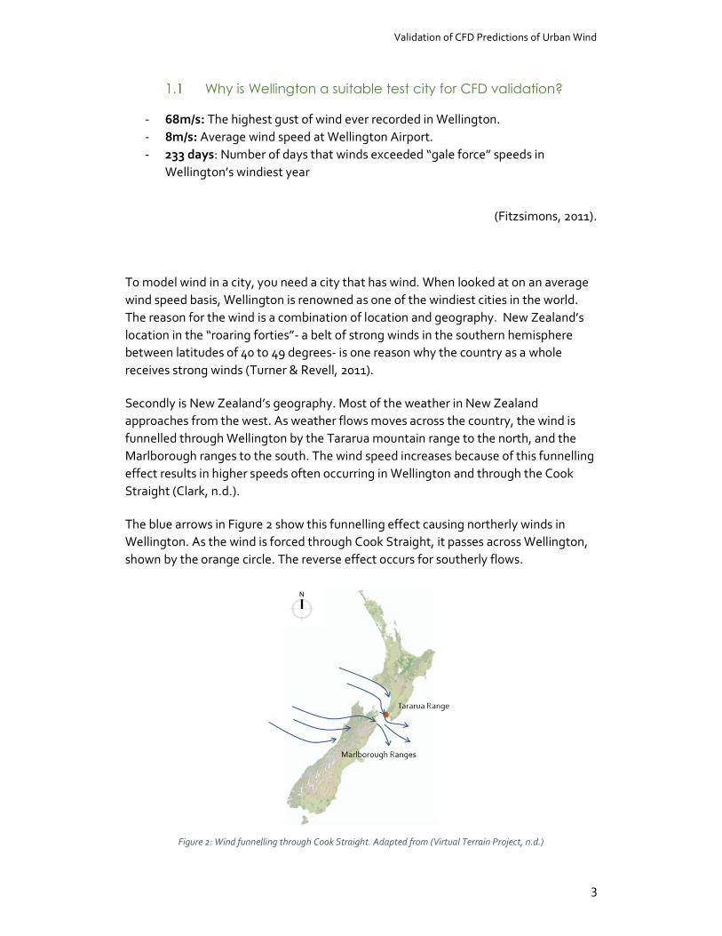
Secondly is New Zealand’s geography. Most of the weather in New Zealand approaches from the west. As weather flows moves across the country, the wind is funnelled through Wellington by the Tararua mountain range to the north, and the Marlborough ranges to the south. The wind speed increases because of this funnelling effect results in higher speeds often occurring in Wellington and through the Cook Straight (Clark, n.d.).
The blue arrows in Figure 2 show this funnelling effect causing northerly winds in Wellington. As the wind is forced through Cook Straight, it passes across Wellington, shown by the orange circle. The reverse effect occurs for southerly flows.
Figure 2: Wind funnelling through Cook Straight. Adapted from (Virtual Terrain Project, n.d.)
Validation of CFD Predictions of Urban Wind
4
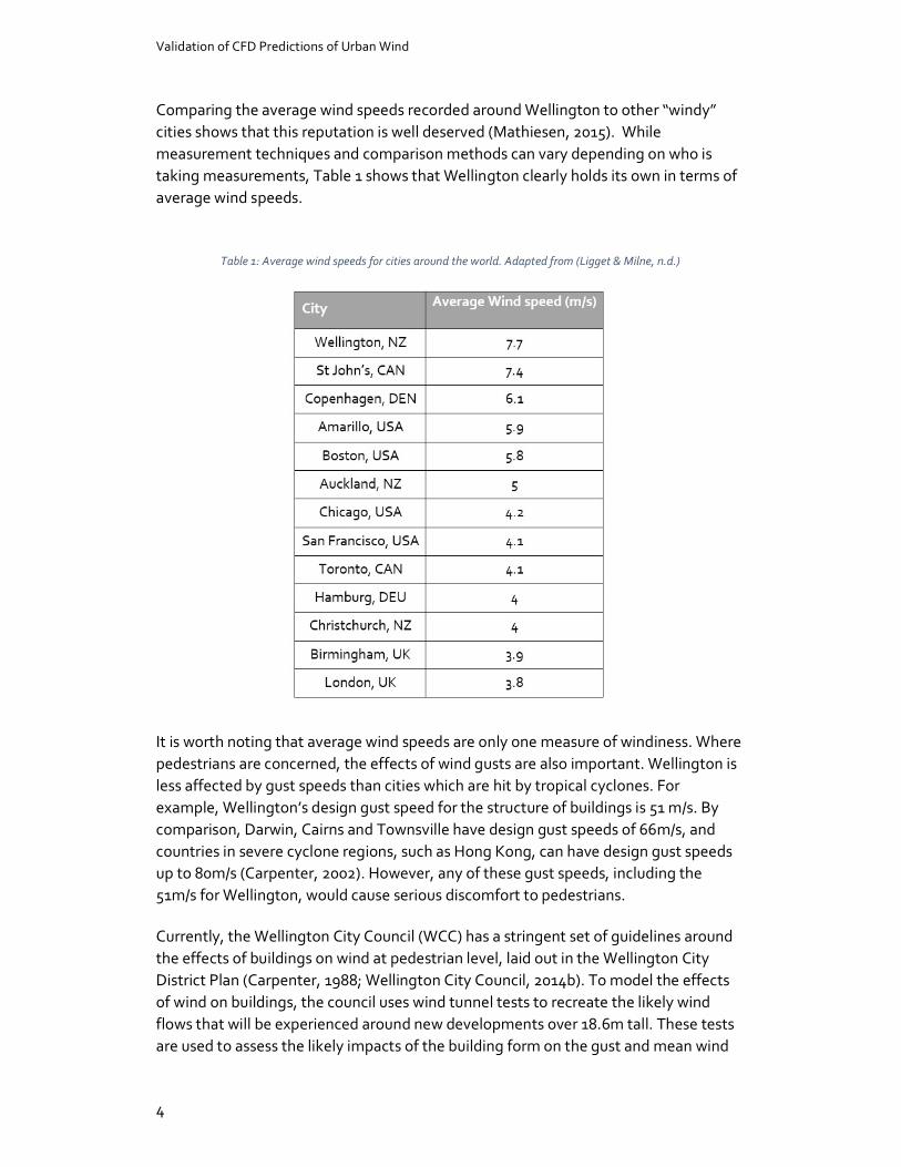
Comparing the average wind speeds recorded around Wellington to other “windy” cities shows that this reputation is well deserved (Mathiesen, 2015). While measurement techniques and comparison methods can vary depending on who is taking measurements, Table 1 shows that Wellington clearly holds its own in terms of average wind speeds.
Table 1: Average wind speeds for cities around the world. Adapted from (Ligget & Milne, n.d.)
It is worth noting that average wind speeds are only one measure of windiness. Where pedestrians are concerned, the effects of wind gusts are also important. Wellington is less affected by gust speeds than cities which are hit by tropical cyclones. For example, Wellington’s design gust speed for the structure of buildings is 51 m/s. By comparison, Darwin, Cairns and Townsville have design gust speeds of 66m/s, and countries in severe cyclone regions, such as Hong Kong, can have design gust speeds up to 80m/s (Carpenter, 2002). However, any of these gust speeds, including the 51m/s for Wellington, would cause serious discomfort to pedestrians.
Currently, the Wellington City Council (WCC) has a stringent set of guidelines around the effects of buildings on wind at pedestrian level, laid out in the Wellington City District Plan (Carpenter, 1988; Wellington City Council, 2014b). To model the effects of wind on buildings, the council uses wind tunnel tests to recreate the likely wind flows that will be experienced around new developments over 18.6m tall. These tests are used to assess the likely impacts of the building form on the gust and mean wind
Validation of CFD Predictions of Urban Wind
5
speeds around the site. Where the wind tunnel predicts the new building could cause high wind speeds which would be unpleasant and potentially dangerous, a new design is required.
The City of London is also investigating alternatives to the current testing process
This is not unique to Wellington. In London, which is shown in Table 1 to have much lower average wind speeds, wind tunnel tests are a standard tool to assess the impact of new tall buildings on the pedestrian wind environment. However, as illustrated by the quote below, wind tunnel tests do not always fully communicate the effect of the building to the designers and planners:
"The wind outcome at street level experienced post-construction on a number of projects differs somewhat to the conditions we were expecting from the ones outlined in the planning application wind assessments," said head of design Gwyn Richards.
"This is why we are asking for an independent verification of the wind studies on a number of new schemes to ensure as rigorous and resilient an approach as possible."
Frearson, 2015. “Walkie Talkie Blamed for Powerful downdraught on London streets”
The building in question is 20 Fenchurch Street, or the “Walkie Talkie” building. As part of the consent application, the building had undergone wind tunnel testing before construction. The wind tunnel tests identified that the building would cause adverse wind conditions around the northwest, southeast and southwest corners of the site. Mitigation strategies that were suggested included planting a combination of tall trees to reduce the overall wind, and low level planting to reduce pedestrian level wind (Aurelius, 2011).
However, the recommendations made in the report were not carried out as intended. This resulted in wind conditions which caused discomfort to pedestrians and people working in the area around the building. In the months following construction, there were media reports of nearby businesses complaining of high winds brought on by the downdraught from the building (Ward, 2015).

Validation of CFD Predictions of Urban Wind
6
CFD could help consultants communicate with designers and planners to properly implement design strategies
The wind conditions around 20 Fenchurch St were not caused by inaccurate modelling, but rather from a lack of understanding in the implementation of wind mitigation strategies. A potential way to reduce these types of misunderstanding is to combine the established methods of wind tunnel reporting with a more visual means of wind prediction. This would allow designers to quickly and easily compare changes to determine which design provides the most comfortable conditions around the site.
One such method of predicting wind is CFD, which provides in-depth analysis of the air movement through and around buildings, using enhanced representation of complex fluid dynamic calculations. Effectively it re-creates a virtual wind tunnel, which can be used to test working design models. In simple terms, it allows designers to understand the effects of different design options in a more detailed way than traditional wind tunnel testing. This allows for more detailed communication of the wind effects resulting from a design, reducing the potential for unclear and confusing test results.
This approach is not novel. To improve the clarity of wind tunnel test results, the City of London now also requires a CFD analysis of all new buildings. Similarly, the Dutch Wind Nuisance Standard NEN8100 allows developers to choose between CFD and wind tunnel tests (Blocken et al., 2016). The successful establishment of CFD in these places suggests that there is potential for it to be implemented in Wellington as well.
However, as with all types of simulation, CFD simulations are only reliable when the results can be validated. Validation is the process that identifies whether a CFD model can be trusted to represent reality, and is the cornerstone of any successful computer analysis. It requires a high-quality data set which can be recreated in the CFD program, and which is representative of the urban geometry that is being assessed.
These requirements form the basis of an investigation into the existing data sets currently used for CFD validation. Most studies that use CFD begin with a validation test, to ensure that the modeller is capable of representing the real-life wind conditions which would be expected (Blocken et al., 2016). The most common form of CFD validation is via comparison with wind tunnel measurements, as wind tunnel test results are seen as a trustworthy benchmark (Carpenter, 2002; Shilston, 2015).
Validation of CFD Predictions of Urban Wind
7
Questions to address
The first part of the research investigates existing datasets and their suitability for use in Wellington based validation test by asking three questions:
1. Do any standardised wind tunnel/full scale data sets exist which are suitable for CFD validation?
2. What are the key aspects of these data sets that make them suitable for CFD validation?
3. Which of the data sets (if any) is the most suitable for use as a standard CFD validation dataset?
These questions are answered in section 2, through a literature review of wind tunnel and CFD studies of urban forms and CFD validation. Once the existence of any validation data sets is established, and the most appropriate data set for CFD validation is determined, the next questions relate to the feasibility of CFD validation of wind flows, specifically for Wellington city:
4. What guidelines exist for CFD validation? Do they provide adequate guidance
for a consultant who understands how wind interacts with buildings, but does not have an in-depth knowledge CFD simulations?
5. What are the requirements for a wind tunnel data set which is representative of the wind flow in a real city, and do any of the existing data sets meet these requirements?
The test of the existing validation guidelines, and whether the existing configurations can be considered representative is detailed in section 3. The results and conclusions drawn from these tests are presented in sections 4 and 5.
Goals
Predicting the wind conditions at street level around buildings is a similar task to what is carried out by wind tunnel assessment for building consents. The goal of this research to investigate the potential for an integrated CFD approach to testing the wind effects of new buildings. If successful, this CFD approach could be used as supplementary information- or even an alternative to wind tunnel modelling- by the Wellington City Council.
8
2. Validation of CFD Predictions of Urban Wind
With Section 1 identifying the need for robust validation of CFD analyses, this chapter investigates the current best practice in proving CFD prediction in urban areas is trustworthy. To do this, the following issues are investigated:
- The current state of CFD validation for urban wind prediction. - What validation data is currently available, and how appropriate this data is for
validation of CFD simulations of urban wind.
The current state of CFD validation for urban wind prediction
Blocken and several co-authors have undertaken a series of recent reviews on the state of Computational Wind Engineering (CWE), which is defined as the use of CFD for wind engineering purposes (Blocken, 2014). Their conclusions is that although constantly improving, CFD simulations are still not viewed as trustworthy without validation against another data source. The most common source for validation data is wind tunnel tests that have been shown to be trustworthy through comparison to real-world measurements (Blocken, 2014; Blocken & Stathopoulos, 2013; Blocken et al., 2016; Ramponi & Blocken, 2012a).

Validation of CFD Predictions of Urban Wind
9
However, though validation is a standard part of most CFD studies, there is no common data set that has been widely used as a comparison against CFD simulations. The upshot of this is that the efficacy of the validation process then becomes heavily dependent on the experience and knowledge of the CFD user (Blocken, 2014).
Indeed, in one study, the authors used wind pressure data from Quan et al., (2007) to validate a study which was comparing wind speeds (Ramponi, Blocken, de Coo, & Janssen, 2015). The paper does not give the reason for doing this when validation datasets which focus on wind speeds, and would therefore have been more applicable, also exist. However, the configuration of blocks used for validation were a better match to the type of study carried out using CFD.
It is possible that the authors believed that the validation configuration having the appropriate form was more important than potential issues matching wind speed to wind pressure data. Unfortunately, the this was not addressed directly, but rather the paper claimed that “Given the strong coupling between the mean velocity field and the mean pressure field, a validation study based on the available pressure coefficients is considered appropriate” (Ramponi et al., 2015).
In this study, the authors happen to be well-published, and have produced numerous research papers investigating the trustworthiness of CFD. With their in-depth understanding of the CFD validation process, their assumption that pressure studies are suitable for the type of CFD validation being carried out is likely to be trustworthy. However, novice CFD users would require some guidance in making similar assumptions when carrying out a validation study. To provide this guidance, a standard validation test approach is required.
A key part of this test approach is finding a trustworthy dataset which can be used to validate CFD simulations. The first research question of this thesis asked whether any standard wind tunnel data sets exist which are suitable for CFD validation.
Validation of CFD Predictions of Urban Wind
10
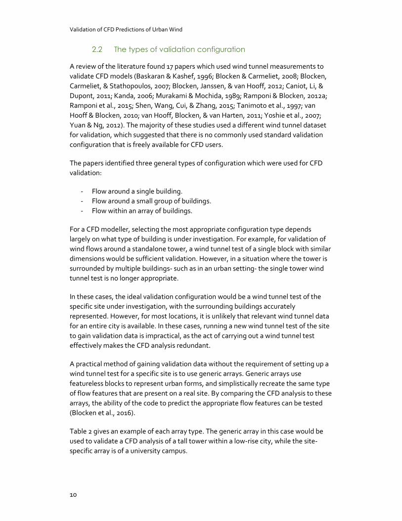
The types of validation configuration
A review of the literature found 17 papers which used wind tunnel measurements to validate CFD models (Baskaran & Kashef, 1996; Blocken & Carmeliet, 2008; Blocken, Carmeliet, & Stathopoulos, 2007; Blocken, Janssen, & van Hooff, 2012; Caniot, Li, & Dupont, 2011; Kanda, 2006; Murakami & Mochida, 1989; Ramponi & Blocken, 2012a; Ramponi et al., 2015; Shen, Wang, Cui, & Zhang, 2015; Tanimoto et al., 1997; van Hooff & Blocken, 2010; van Hooff, Blocken, & van Harten, 2011; Yoshie et al., 2007; Yuan & Ng, 2012). The majority of these studies used a different wind tunnel dataset for validation, which suggested that there is no commonly used standard validation configuration that is freely available for CFD users.
The papers identified three general types of configuration which were used for CFD validation:
- Flow around a single building. - Flow around a small group of buildings. - Flow within an array of buildings.
For a CFD modeller, selecting the most appropriate configuration type depends largely on what type of building is under investigation. For example, for validation of wind flows around a standalone tower, a wind tunnel test of a single block with similar dimensions would be sufficient validation. However, in a situation where the tower is surrounded by multiple buildings- such as in an urban setting- the single tower wind tunnel test is no longer appropriate.
In these cases, the ideal validation configuration would be a wind tunnel test of the specific site under investigation, with the surrounding buildings accurately represented. However, for most locations, it is unlikely that relevant wind tunnel data for an entire city is available. In these cases, running a new wind tunnel test of the site to gain validation data is impractical, as the act of carrying out a wind tunnel test effectively makes the CFD analysis redundant.
A practical method of gaining validation data without the requirement of setting up a wind tunnel test for a specific site is to use generic arrays. Generic arrays use featureless blocks to represent urban forms, and simplistically recreate the same type of flow features that are present on a real site. By comparing the CFD analysis to these arrays, the ability of the code to predict the appropriate flow features can be tested (Blocken et al., 2016).
Table 2 gives an example of each array type. The generic array in this case would be used to validate a CFD analysis of a tall tower within a low-rise city, while the site-specific array is of a university campus.
Validation of CFD Predictions of Urban Wind
11
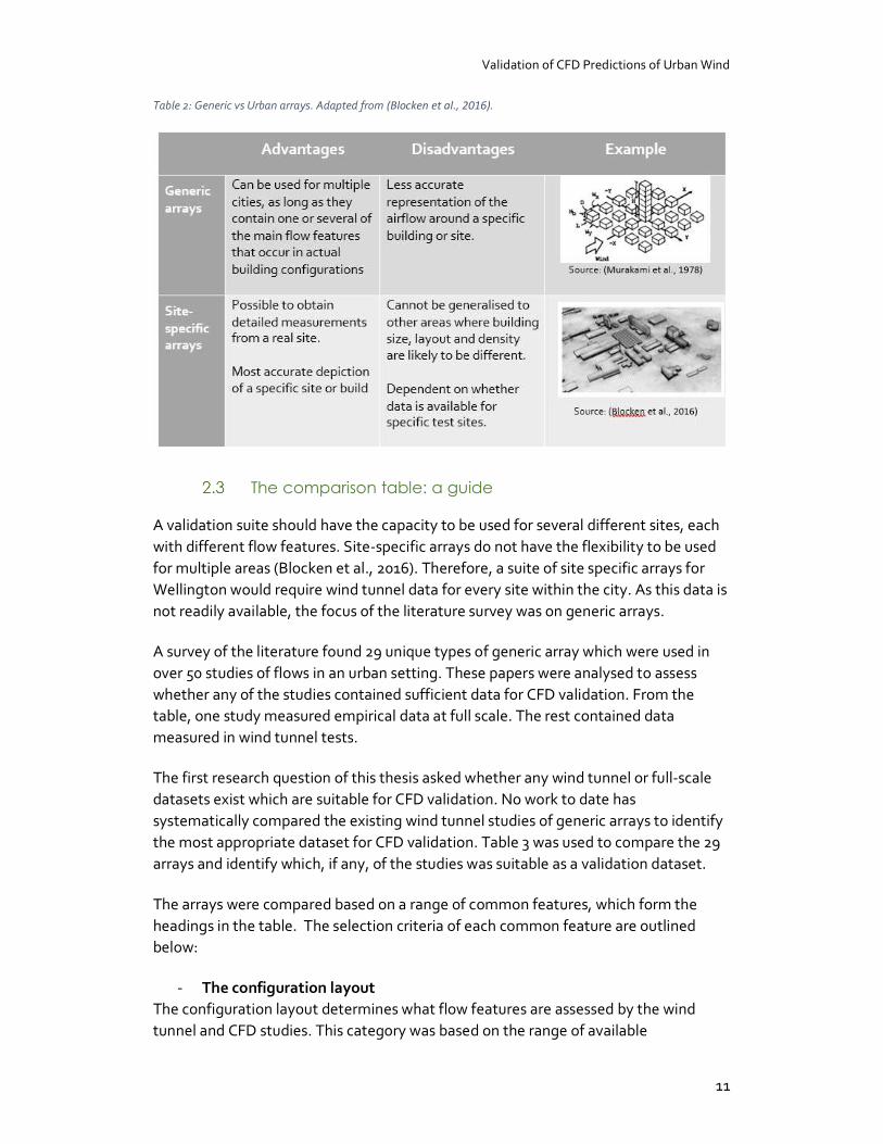
Table 2: Generic vs Urban arrays. Adapted from (Blocken et al., 2016).
The comparison table: a guide
A validation suite should have the capacity to be used for several different sites, each with different flow features. Site-specific arrays do not have the flexibility to be used for multiple areas (Blocken et al., 2016). Therefore, a suite of site specific arrays for Wellington would require wind tunnel data for every site within the city. As this data is not readily available, the focus of the literature survey was on generic arrays.
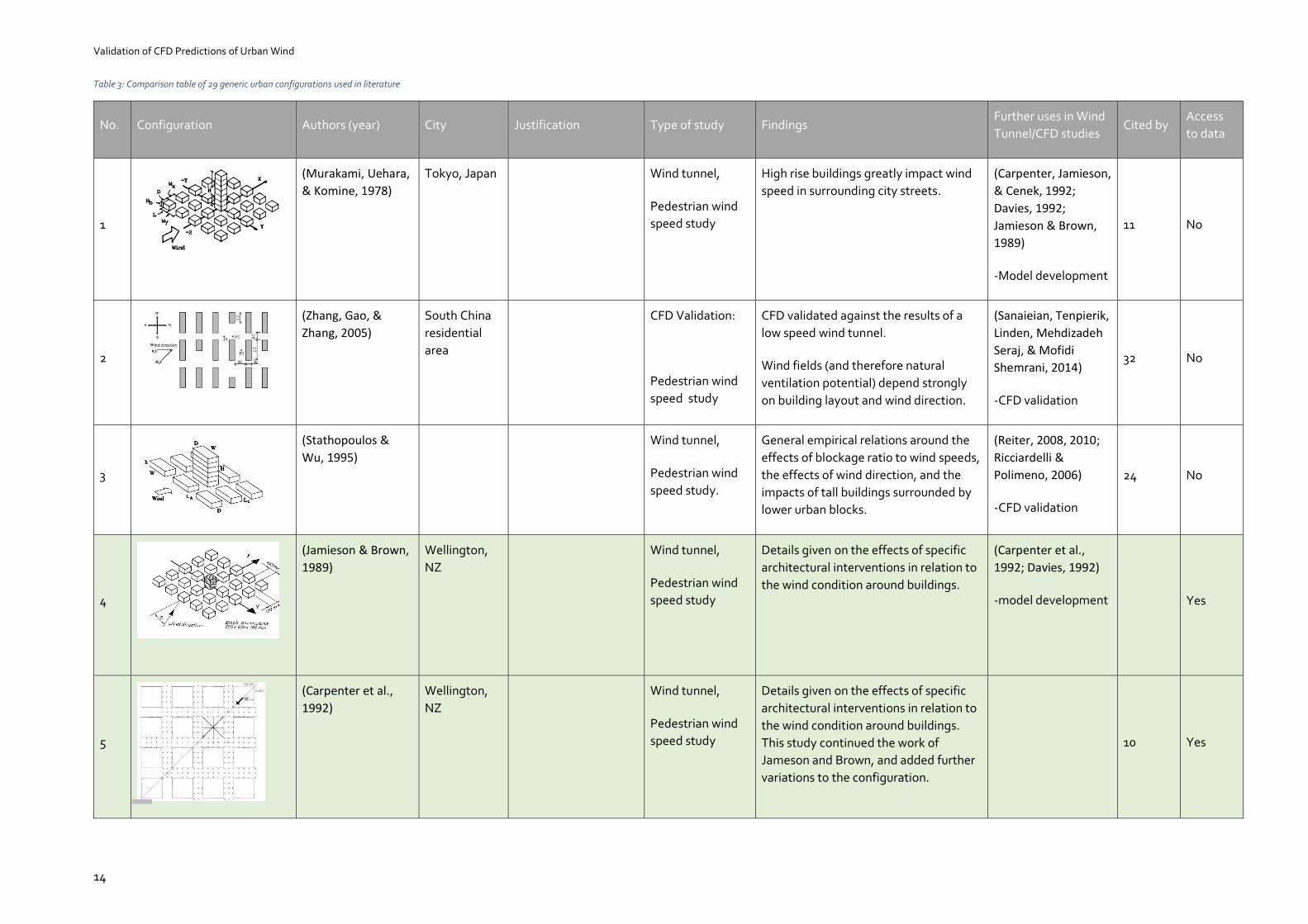
A survey of the literature found 29 unique types of generic array which were used in over 50 studies of flows in an urban setting. These papers were analysed to assess whether any of the studies contained sufficient data for CFD validation. From the table, one study measured empirical data at full scale. The rest contained data measured in wind tunnel tests.
The first research question of this thesis asked whether any wind tunnel or full-scale datasets exist which are suitable for CFD validation. No work to date has systematically compared the existing wind tunnel studies of generic arrays to identify the most appropriate dataset for CFD validation. Table 3 was used to compare the 29 arrays and identify which, if any, of the studies was suitable as a validation dataset.
The arrays were compared based on a range of common features, which form the headings in the table. The selection criteria of each common feature are outlined below:
- The configuration layout The configuration layout determines what flow features are assessed by the wind tunnel and CFD studies. This category was based on the range of available
Validation of CFD Predictions of Urban Wind
12
configurations with the dataset, as well as how relevant the forms in the configuration were to Wellington city.
- Study author and year The author and date were included to reference the paper that the configuration was found in. Where possible, the earliest recorded use of each configuration was included, as the paper where the configuration was designed was most likely to have some justification for the forms used.
- City Where the paper identified which city was supposed to be represented by the generic array, this information was recorded. The cities were included so as to link to the justification of the forms used.
- Justification In terms of collecting trustworthy results, this was the most important category. Configurations which contained a robust justification for the chosen form were highlighted grey in the table. The justification category looked for an explanation of why the configuration consisted of the chosen forms. If a paper had a good justification for its configuration, the results of the wind tunnel tests could be generalised to the conditions in the city that was being represented.
For example, a single tall tower amongst smaller blocks is justified as a model if it is representing a new high-rise apartment in a traditionally low-rise city. However, without this justification, the 3D geometry is difficult to relate to actual city conditions.
- Type of study This category identified whether the paper was focussed on the wind tunnel results, or was also being used as a CFD validation study. The focus of each paper was divided into three categories. The first were pedestrian wind speed studies, which focussed on wind speeds in urban environments. Secondly were wind profile studies, which investigated the effect of different urban configurations on the local wind climate. Lastly were pollutant dispersal studies, which focussed on the wind effects on pollutants in the urban environment
- Findings of the study The findings of each study were briefly summarised. This category was used to identify whether geometry was considered in the aims of each study.

Validation of CFD Predictions of Urban Wind
13
- Further uses in wind tunnel/CFD studies Many of the configurations identified in the table were used by other authors for future studies, often as CFD validation. Where available, the papers which had used the same configuration were recorded.
- Cited by This category determined how many authors had cited the study.
- Access to data Overall, access to data was the most important criteria which determined whether a configuration could be used. The datasets which provided access to the measured data were highlighted green.
Validation of CFD Predictions of Urban Wind
14
Table 3: Comparison table of 29 generic urban configurations used in literature
No. Configuration Authors (year) City Justification Type of study Findings Further uses in Wind Tunnel/CFD studies
Cited by Access to data
1
(Murakami, Uehara, & Komine, 1978)
Tokyo, Japan Wind tunnel,
Pedestrian wind speed study
High rise buildings greatly impact wind speed in surrounding city streets.
(Carpenter, Jamieson, & Cenek, 1992; Davies, 1992; Jamieson & Brown, 1989)
-Model development
11 No
2
(Zhang, Gao, & Zhang, 2005)
South China residential area
CFD Validation:
Pedestrian wind speed study
CFD validated against the results of a low speed wind tunnel.
Wind fields (and therefore natural ventilation potential) depend strongly on building layout and wind direction.
(Sanaieian, Tenpierik, Linden, Mehdizadeh Seraj, & Mofidi Shemrani, 2014)
-CFD validation
32 No
3
(Stathopoulos & Wu, 1995)
Wind tunnel,
Pedestrian wind speed study.
General empirical relations around the effects of blockage ratio to wind speeds, the effects of wind direction, and the impacts of tall buildings surrounded by lower urban blocks.
(Reiter, 2008, 2010; Ricciardelli & Polimeno, 2006)
-CFD validation
24 No
4
(Jamieson & Brown, 1989)
Wellington, NZ
Wind tunnel,
Pedestrian wind speed study
Details given on the effects of specific architectural interventions in relation to the wind condition around buildings.
(Carpenter et al., 1992; Davies, 1992)
-model development Yes
5
(Carpenter et al., 1992)
Wellington, NZ
Wind tunnel,
Pedestrian wind speed study
Details given on the effects of specific architectural interventions in relation to the wind condition around buildings. This study continued the work of Jameson and Brown, and added further variations to the configuration.
10 Yes
Validation of CFD Predictions of Urban Wind
15
No. Configuration Authors (year) City Justification Type of study Findings Further uses in Wind Tunnel/CFD studies
Cited by Access to data
6
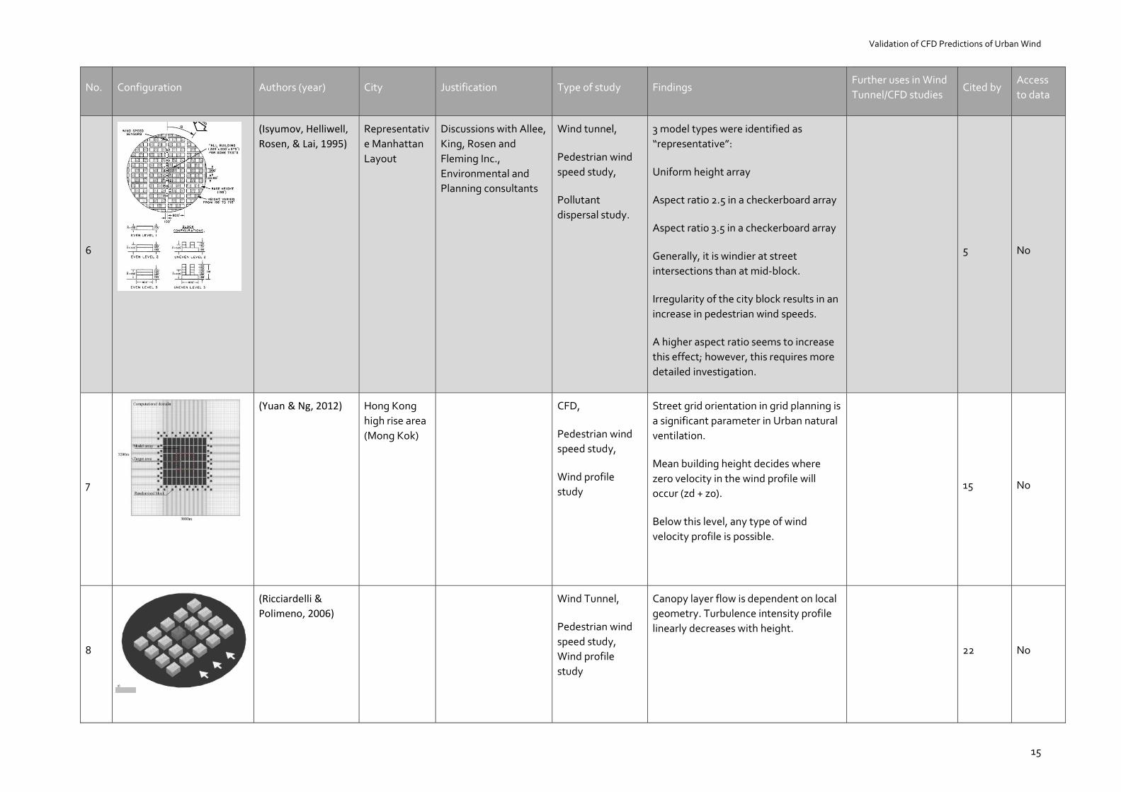
(Isyumov, Helliwell, Rosen, & Lai, 1995)
Representative Manhattan Layout
Discussions with Allee, King, Rosen and Fleming Inc., Environmental and Planning consultants
Wind tunnel,
Pedestrian wind speed study,
Pollutant dispersal study.
3 model types were identified as “representative”:
Uniform height array
Aspect ratio 2.5 in a checkerboard array
Aspect ratio 3.5 in a checkerboard array
Generally, it is windier at street intersections than at mid-block.
Irregularity of the city block results in an increase in pedestrian wind speeds.
A higher aspect ratio seems to increase this effect; however, this requires more detailed investigation.
5 No
7
(Yuan & Ng, 2012) Hong Kong high rise area (Mong Kok)
CFD,
Pedestrian wind speed study,
Wind profile study
Street grid orientation in grid planning is a significant parameter in Urban natural ventilation.
Mean building height decides where zero velocity in the wind profile will occur (zd + z0).
Below this level, any type of wind velocity profile is possible.
15 No
8
(Ricciardelli & Polimeno, 2006)
Wind Tunnel,
Pedestrian wind speed study, Wind profile study
Canopy layer flow is dependent on local geometry. Turbulence intensity profile linearly decreases with height.
22 No
Validation of CFD Predictions of Urban Wind
16
No. Configuration Authors (year) City Justification Type of study Findings Further uses in Wind Tunnel/CFD studies
Cited by Access to data
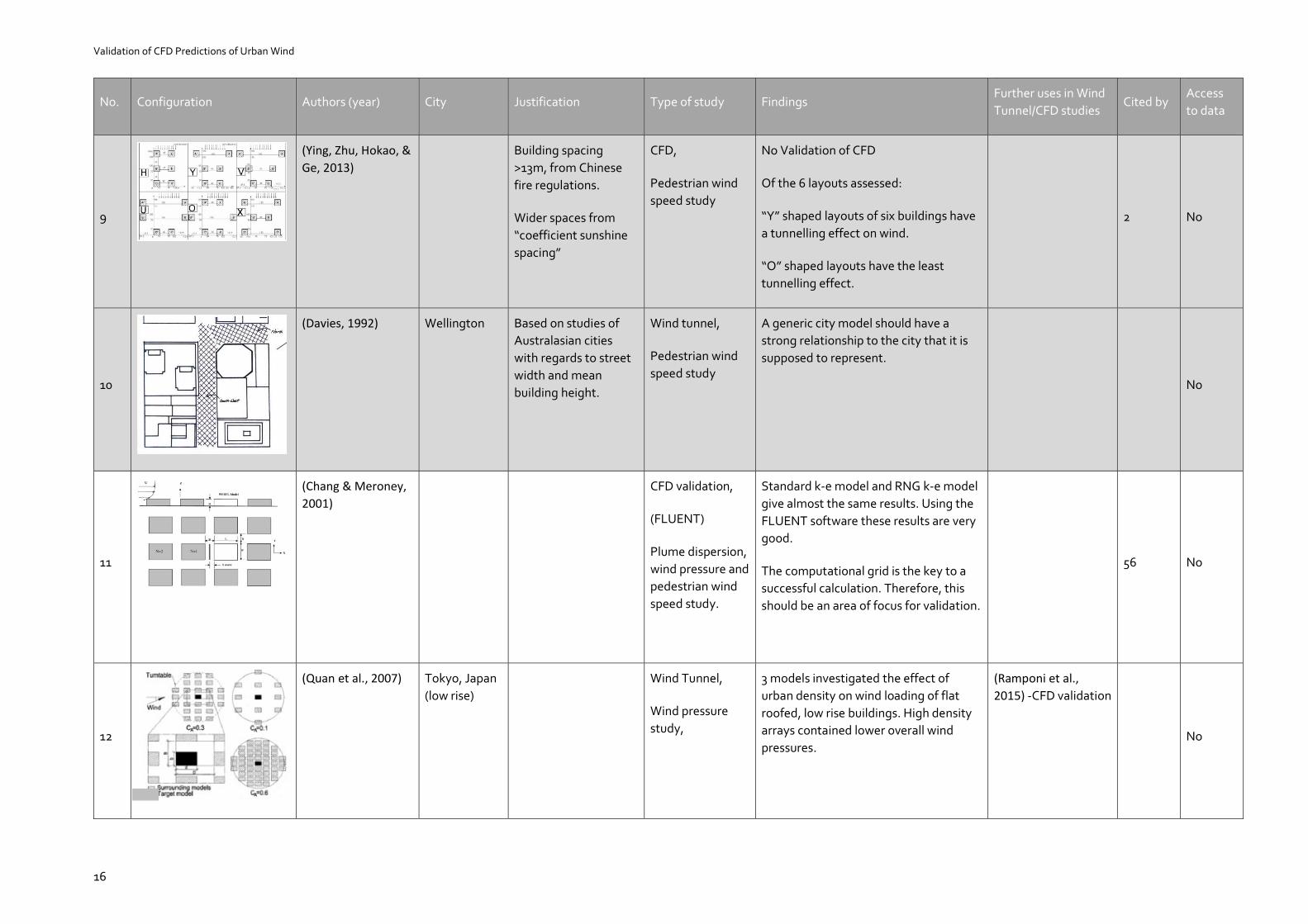
9
(Ying, Zhu, Hokao, & Ge, 2013)
Building spacing >13m, from Chinese fire regulations.
Wider spaces from “coefficient sunshine spacing”
CFD,
Pedestrian wind speed study
No Validation of CFD
Of the 6 layouts assessed:
“Y” shaped layouts of six buildings have a tunnelling effect on wind.
“O” shaped layouts have the least tunnelling effect.
2 No
10
(Davies, 1992) Wellington Based on studies of Australasian cities with regards to street width and mean building height.
Wind tunnel,
Pedestrian wind speed study
A generic city model should have a strong relationship to the city that it is supposed to represent.
No
11
(Chang & Meroney, 2001)
CFD validation,
(FLUENT)
Plume dispersion, wind pressure and pedestrian wind speed study.
Standard k-e model and RNG k-e model give almost the same results. Using the FLUENT software these results are very good.
The computational grid is the key to a successful calculation. Therefore, this should be an area of focus for validation.
56 No
12
(Quan et al., 2007) Tokyo, Japan (low rise)
Wind Tunnel,
Wind pressure study,
3 models investigated the effect of urban density on wind loading of flat roofed, low rise buildings. High density arrays contained lower overall wind pressures.
(Ramponi et al., 2015) -CFD validation
No
Validation of CFD Predictions of Urban Wind
17
No. Configuration Authors (year) City Justification Type of study Findings Further uses in Wind
Tunnel/CFD studies Cited by
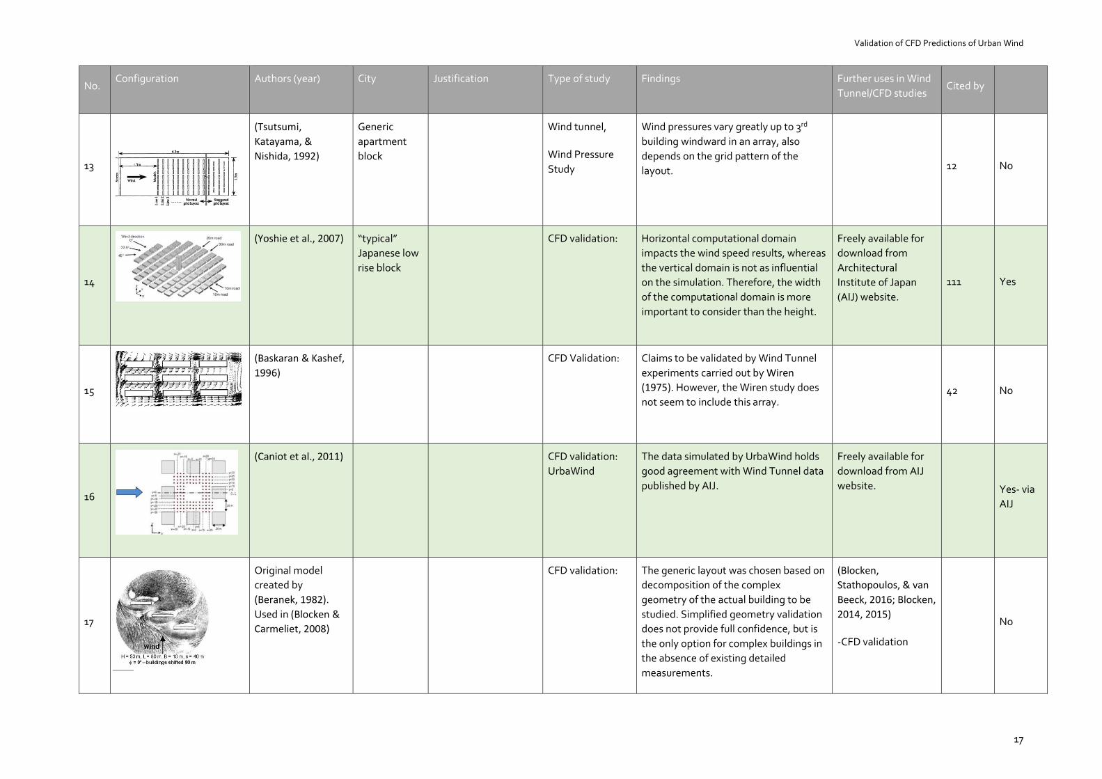
13
(Tsutsumi, Katayama, & Nishida, 1992)
Generic apartment block
Wind tunnel,
Wind Pressure Study
Wind pressures vary greatly up to 3rd building windward in an array, also depends on the grid pattern of the layout.
12 No
14
(Yoshie et al., 2007) “typical” Japanese low rise block
CFD validation: Horizontal computational domain impacts the wind speed results, whereas the vertical domain is not as influential on the simulation. Therefore, the width of the computational domain is more important to consider than the height.
Freely available for download from Architectural Institute of Japan (AIJ) website.
111 Yes
15
(Baskaran & Kashef, 1996)
CFD Validation:
Claims to be validated by Wind Tunnel experiments carried out by Wiren (1975). However, the Wiren study does not seem to include this array.
42 No
16
(Caniot et al., 2011) CFD validation: UrbaWind
The data simulated by UrbaWind holds good agreement with Wind Tunnel data published by AIJ.
Freely available for download from AIJ website.
Yes- via AIJ
17
Original model created by (Beranek, 1982). Used in (Blocken & Carmeliet, 2008)
CFD validation: The generic layout was chosen based on decomposition of the complex geometry of the actual building to be studied. Simplified geometry validation does not provide full confidence, but is the only option for complex buildings in the absence of existing detailed measurements.
(Blocken, Stathopoulos, & van Beeck, 2016; Blocken, 2014, 2015)
-CFD validation
No
Validation of CFD Predictions of Urban Wind
18
No. Configuration Authors (year) City Justification Type of study Findings Further uses in Wind Tunnel/CFD studies
Cited by Access to data
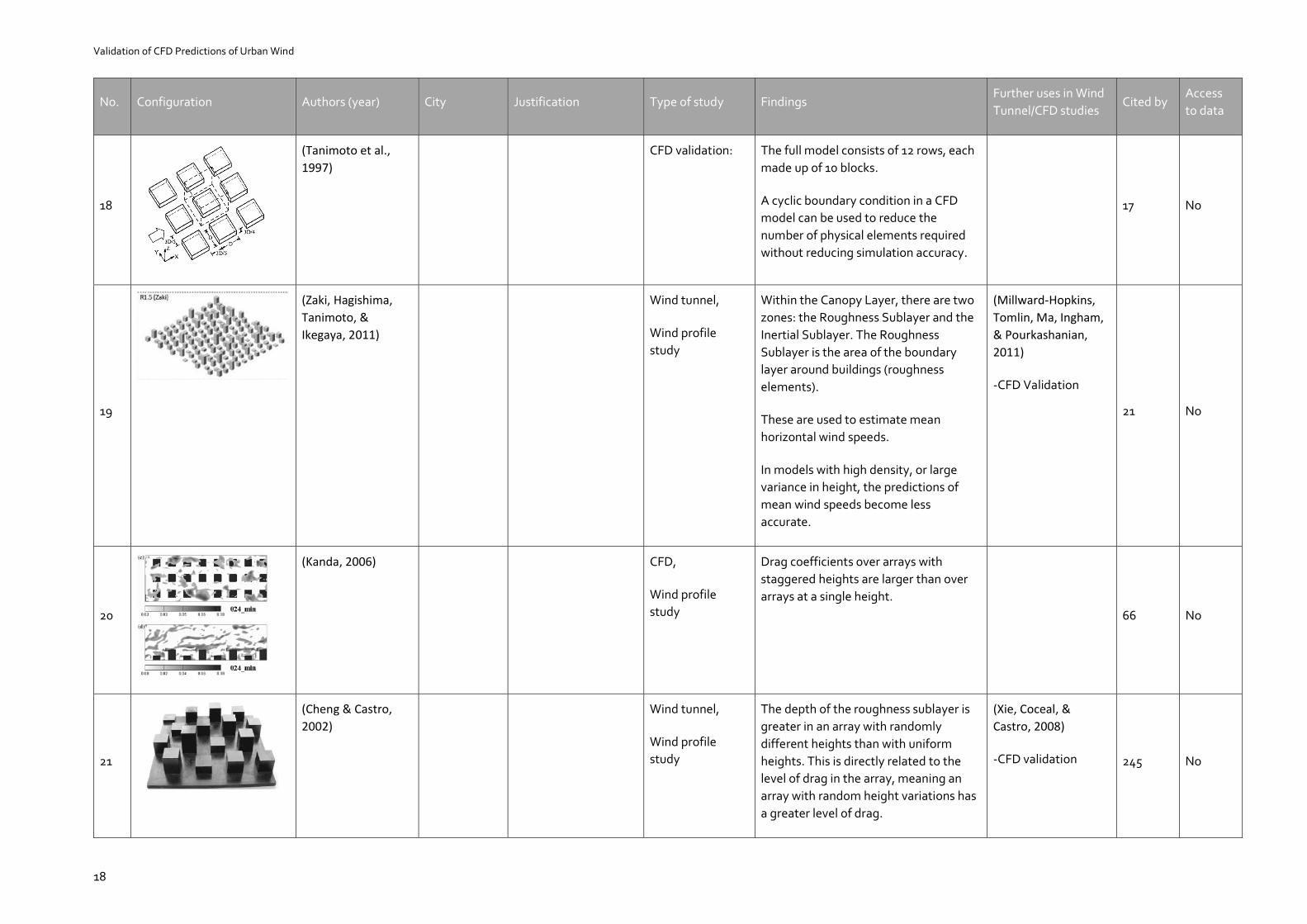
18
(Tanimoto et al., 1997)
CFD validation: The full model consists of 12 rows, each made up of 10 blocks.
A cyclic boundary condition in a CFD model can be used to reduce the number of physical elements required without reducing simulation accuracy.
17 No
19
(Zaki, Hagishima, Tanimoto, & Ikegaya, 2011)
Wind tunnel,
Wind profile study
Within the Canopy Layer, there are two zones: the Roughness Sublayer and the Inertial Sublayer. The Roughness Sublayer is the area of the boundary layer around buildings (roughness elements).
These are used to estimate mean horizontal wind speeds.
In models with high density, or large variance in height, the predictions of mean wind speeds become less accurate.
(Millward-Hopkins, Tomlin, Ma, Ingham, & Pourkashanian, 2011)
-CFD Validation
21 No
20
(Kanda, 2006) CFD,
Wind profile study
Drag coefficients over arrays with staggered heights are larger than over arrays at a single height.
66 No
21
(Cheng & Castro, 2002)
Wind tunnel,
Wind profile study
The depth of the roughness sublayer is greater in an array with randomly different heights than with uniform heights. This is directly related to the level of drag in the array, meaning an array with random height variations has a greater level of drag.
(Xie, Coceal, & Castro, 2008)
-CFD validation 245 No
Validation of CFD Predictions of Urban Wind
19
No. Configuration Authors (year) City Justification Type of study Findings Further uses in Wind Tunnel/CFD studies
Cited by Access to data
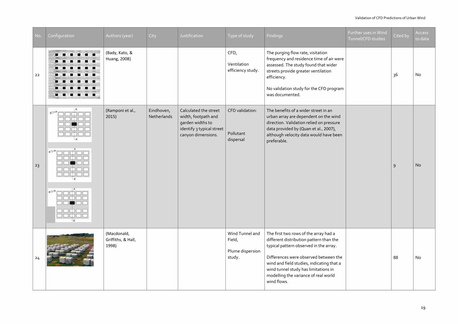
22
(Bady, Kato, & Huang, 2008)
CFD,
Ventilation efficiency study.
The purging flow rate, visitation frequency and residence time of air were assessed. The study found that wider streets provide greater ventilation efficiency.
No validation study for the CFD program was documented.
36 No
23
(Ramponi et al., 2015)
Eindhoven, Netherlands
Calculated the street width, footpath and garden widths to identify 3 typical street canyon dimensions.
CFD validation:
Pollutant dispersal
The benefits of a wider street in an urban array are dependent on the wind direction. Validation relied on pressure data provided by (Quan et al., 2007), although velocity data would have been preferable.
9 No
24
(Macdonald, Griffiths, & Hall, 1998)
Wind Tunnel and Field,
Plume dispersion study.
The first two rows of the array had a different distribution pattern than the typical pattern observed in the array.
Differences were observed between the wind and field studies, indicating that a wind tunnel study has limitations in modelling the variance of real world wind flows.
88 No
Validation of CFD Predictions of Urban Wind
20
No. Configuration Authors (year) City Justification Type of study Findings Further uses in Wind Tunnel/CFD studies
Cited by Access to data
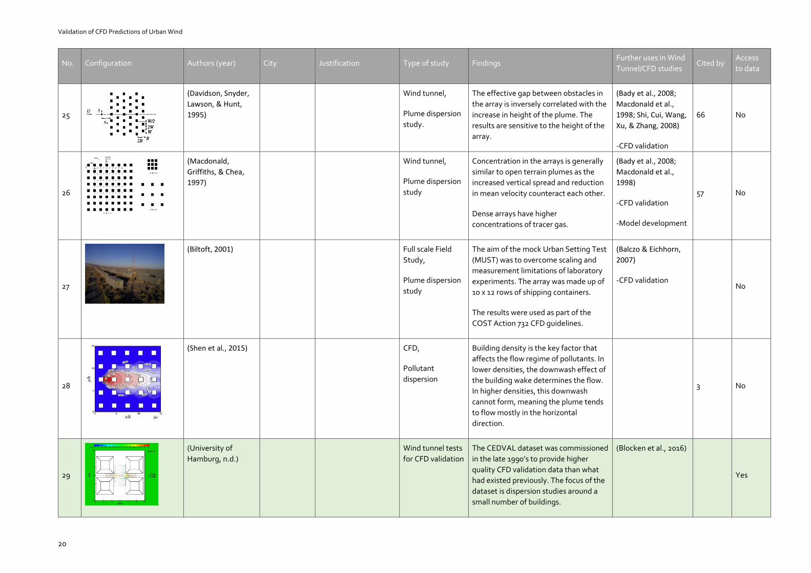
25
(Davidson, Snyder, Lawson, & Hunt, 1995)
Wind tunnel,
Plume dispersion study.
The effective gap between obstacles in the array is inversely correlated with the increase in height of the plume. The results are sensitive to the height of the array.
(Bady et al., 2008; Macdonald et al., 1998; Shi, Cui, Wang, Xu, & Zhang, 2008)
-CFD validation
66 No
26
(Macdonald, Griffiths, & Chea, 1997)
Wind tunnel,
Plume dispersion study
Concentration in the arrays is generally similar to open terrain plumes as the increased vertical spread and reduction in mean velocity counteract each other.
Dense arrays have higher concentrations of tracer gas.
(Bady et al., 2008; Macdonald et al., 1998)
-CFD validation
-Model development
57 No
27
(Biltoft, 2001) Full scale Field Study,
Plume dispersion study
The aim of the mock Urban Setting Test (MUST) was to overcome scaling and measurement limitations of laboratory experiments. The array was made up of 10 x 12 rows of shipping containers.
The results were used as part of the COST Action 732 CFD guidelines.
(Balczo & Eichhorn, 2007)
-CFD validation No
28
(Shen et al., 2015) CFD,
Pollutant dispersion
Building density is the key factor that affects the flow regime of pollutants. In lower densities, the downwash effect of the building wake determines the flow. In higher densities, this downwash cannot form, meaning the plume tends to flow mostly in the horizontal direction.
3 No
29
(University of Hamburg, n.d.)
Wind tunnel tests for CFD validation
The CEDVAL dataset was commissioned in the late 1990’s to provide higher quality CFD validation data than what had existed previously. The focus of the dataset is dispersion studies around a small number of buildings.
(Blocken et al., 2016)
Yes

Validation of CFD Predictions of Urban Wind
21
Findings from the comparison table
The purpose of this table was to systematically analyse the urban forms used in these validation studies. It assigns a ranking according to criteria that measure each study's suitability for use in validation of CFD for use in urban studies. To be suitable, the configuration needed to provide access to a high-quality data set, as well as being designed to represent wind flow features typical of a city. With these requirements, the following conclusions were drawn:
2.4.1 Access to data is a major limitation The most significant finding from the table was that of the 29 configurations, measured data was only available from five studies. However, the configurations used in the five studies came from three separate validation sets, meaning that effectively only three sets were identified. The sets are:
o The Architectural institute of Japan (AIJ dataset) o The CEDVAL set, published by the University of Hamburg, and o The Wellington Standard City dataset, used by (Carpenter et al., 1992)
Data for the AIJ and CEDVAL sets came from publicly accessible online databases, while data from the final model was supplied through contact with one of the authors of the Carpenter et al., (1992) paper. However, gaining access to other data sets from the literature was not straightforward. Several requests were made via email to access the data necessary for CFD validation from the authors of other studies, but no responses were received.
2.4.2 Very few studies consider justifying how the model is “representative” of a real city to be important.
The lack of available data links into the second most significant finding from the comparison table: that very few datasets provided justification for the 3D geometry used. None of the configurations which provided data had any justification relating the 3D geometry to real city forms. This lack of justification makes it difficult for a consultant to generalise the flow features in the array to real cities.
The arrays which did include some justification of the selected geometry discussed two key characteristics. These were:
Validation of CFD Predictions of Urban Wind
22
o Building Height: Street Width ratio- the height to street width ratio has a significant effect on the wind conditions within the generic arrays. The effects of street width to building height ratio were investigated in studies 10, 12, 22, 23, and 26. The studies each concluded that block configurations which had narrow streets produced lower wind velocities than configurations with wider streets. This suggests that a generic array should have a similar block height to street width ratio as the urban area that the configuration is being used to represent.
o Grid layouts that are typical of a real city: City grids are dependent on the location, age and type of urban area. This should be considered when designing a representative configuration.
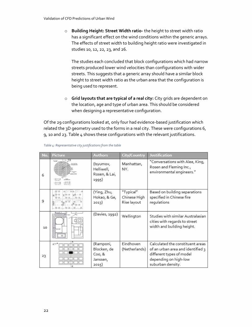
Of the 29 configurations looked at, only four had evidence-based justification which related the 3D geometry used to the forms in a real city. These were configurations 6, 9, 10 and 23. Table 4 shows these configurations with the relevant justifications.
Table 4: Representative city justifications from the table
Validation of CFD Predictions of Urban Wind
23
The two strongest justifications were found in the Davies and the Ramponi et al. studies (Numbers 10 and 23). Some justification had been attempted in the other two studies, however the links between the configurations and the real city geometry were tenuous. In most other studies, the geometry that was used was accepted as representative of a city without any justification.
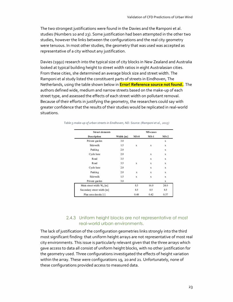
Davies (1992) research into the typical size of city blocks in New Zealand and Australia looked at typical building height to street width ratios in eight Australasian cities. From these cities, she determined an average block size and street width. The Ramponi et al study listed the constituent parts of streets in Eindhoven, The Netherlands, using the table shown below in Error! Reference source not found.. The authors defined wide, medium and narrow streets based on the make-up of each street type, and assessed the effects of each street width on pollutant removal. Because of their efforts in justifying the geometry, the researchers could say with greater confidence that the results of their studies would be replicated in real-world situations.
Table 5:make-up of urban streets in Eindhoven, ND. Source: (Ramponi et al., 2015)
2.4.3 Uniform height blocks are not representative of most real-world urban environments.
The lack of justification of the configuration geometries links strongly into the third most significant finding: that uniform height arrays are not representative of most real city environments. This issue is particularly relevant given that the three arrays which gave access to data all consist of uniform height blocks, with no other justification for the geometry used. Three configurations investigated the effects of height variation within the array. These were configurations 19, 20 and 21. Unfortunately, none of these configurations provided access to measured data.
Validation of CFD Predictions of Urban Wind
24
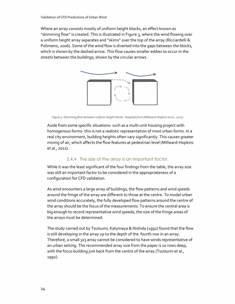
Where an array consists mostly of uniform height blocks, an effect known as “skimming flow” is created. This is illustrated in Figure 3, where the wind flowing over a uniform height array separates and “skims” over the top of the array (Ricciardelli & Polimeno, 2006). Some of the wind flow is diverted into the gaps between the blocks, which is shown by the dashed arrow. This flow causes smaller eddies to occur in the streets between the buildings, shown by the circular arrows.
Figure 3: Skimming flow between uniform height blocks. Adapted from (Millward-Hopkins et al., 2011)
Aside from some specific situations- such as a multi-unit housing project with homogenous forms- this is not a realistic representation of most urban forms. In a real city environment, building heights often vary significantly. This causes greater mixing of air, which affects the flow features at pedestrian level (Millward-Hopkins et al., 2011).
2.4.4 The size of the array is an important factor.
While it was the least significant of the four findings from the table, the array size was still an important factor to be considered in the appropriateness of a configuration for CFD validation.
As wind encounters a large array of buildings, the flow patterns and wind speeds around the fringe of the array are different to those at the centre. To model urban wind conditions accurately, the fully developed flow patterns around the centre of the array should be the focus of the measurements. To ensure the central area is big enough to record representative wind speeds, the size of the fringe areas of the arrays must be determined.
The study carried out by Tsutsumi, Katymaya & Nishida (1992) found that the flow is still developing in the array up to the depth of the fourth row in an array. Therefore, a small 3x3 array cannot be considered to have winds representative of an urban setting. The recommended array size from the paper is 10 rows deep, with the focus building just back from the centre of the array (Tsutsumi et al., 1992).
Validation of CFD Predictions of Urban Wind
25
What is the significance of these findings?
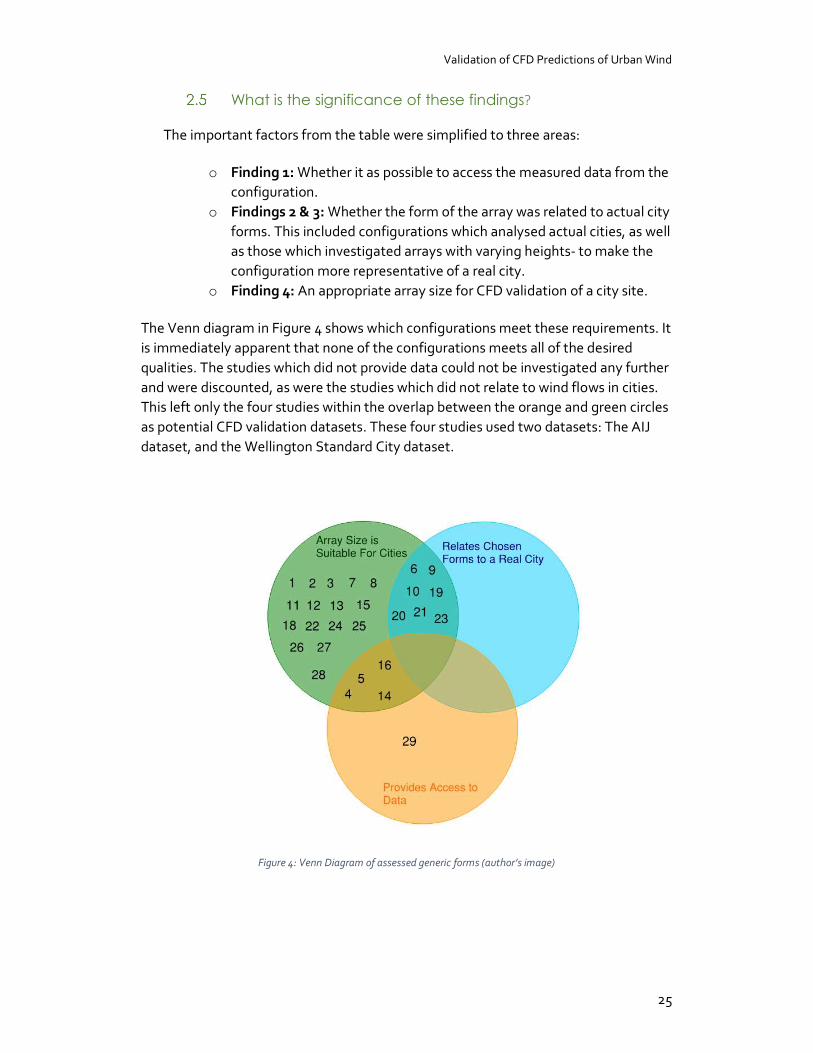
The important factors from the table were simplified to three areas:
o Finding 1: Whether it as possible to access the measured data from the configuration.
o Findings 2 & 3: Whether the form of the array was related to actual city forms. This included configurations which analysed actual cities, as well as those which investigated arrays with varying heights- to make the configuration more representative of a real city.
o Finding 4: An appropriate array size for CFD validation of a city site.
The Venn diagram in Figure 4 shows which configurations meet these requirements. It is immediately apparent that none of the configurations meets all of the desired qualities. The studies which did not provide data could not be investigated any further and were discounted, as were the studies which did not relate to wind flows in cities. This left only the four studies within the overlap between the orange and green circles as potential CFD validation datasets. These four studies used two datasets: The AIJ dataset, and the Wellington Standard City dataset.
Figure 4: Venn Diagram of assessed generic forms (author’s image)
Validation of CFD Predictions of Urban Wind
26
Which configurations are viable CFD validation sets?
2.6.1 Configurations 14 & 16: The AIJ dataset
The first set, available through the AIJ website, consists of a range of simple forms for CFD validation. The set consists of:
Flow around a single 2:1:1 block Flow around a single 4:4:1 block Flow through a 3 x 3 array of uniform height blocks Flow through a tall tower in a uniform height block city Building complexes with simple shape in actual urban area (Niigata) Building complexes with complicated building shape in actual urban area
(Shinjuku)
Single block dimensions are given in height x width x depth format. Of the two datasets that are available, the data in the AIJ set is the most detailed. This is a key consideration for CFD validation, as a highly-detailed data set is integral for reducing the error involved in setting up, running, and validating CFD simulations. The AIJ also published a document which details examples of CFD validation for each configuration, as a guide for practitioners looking to recreate the results.
With the goal of this thesis being to identify an appropriate validation suite for CFD simulations in Wellington, the AIJ dataset contains several configurations which would not be suitable as part of a validation suite:
Both single block sets are not representative of flow through a city. The single block sets are more useful as a simple test, which could be a first step to ensuring that the CFD model can at least predict simple flows before investing the time and effort required for modelling complex city flows.
The 3x3 grid is not large enough to provide fully developed wind flow (Tsutsumi et al., 1992),
The actual urban area sets contain wind flows which are specific to one area, but which can not necessarily be generalised to the flows found around Wellington.
Therefore, the remaining candidate for the validation suite is the tall tower in a low rise city model.

Validation of CFD Predictions of Urban Wind
27
2.6.2 Configuration 4: The Wellington “Standard City” set
Access to the second dataset was provided by Opus Laboratories in Wellington. The Standard City dataset consists of flow measurements through an array of uniform height buildings (60m x 60m x 30m), with one interchangeable central block which is used to assess the difference of the wind effects. The different central block arrangements are:
Uniform Double height block (60m x 60m x 60m) Double height block with upstand and verandah Tall tower (30m x 30m x 240m) Tall tower with 3m high, 35% porous fence 15m from the tower’s base. Octagonal block (60m x 60m x 72m) 48m x 48m x 60m block with balconies at 6m high projections “carpark”- 60m x 60m x 60m block with 50% open area in elevation at 6m
intervals. Tall tower with podium: 30m x 30m x 180m tall tower on a 60m x 60m x 15m
podium.
While it is not publicly available like the AIJ data sets, the Wellington Standard City has the benefit of providing measured flow features for a range of building shapes. Each configuration in the Standard City dataset was designed to model the flows in a city environment. In terms of a validation suite, this is a significant benefit over the AIJ dataset, where only 1 configuration was suited to the CFD validation suite.
However, the Standard City data set was not designed specifically for CFD validation, therefore the data was not as detailed as that provided by the AIJ. Where the AIJ set came with a clearly defined wind profile, clear measurement dimensions and a full document set detailing example CFD validation studies, the Standard City set was provided purely as measurements.
For the wind profile, the mathematical model of wind designed by Deaves & Harris was used (1978). The same testing methodology that was used for the AIJ configuration was applied to the Standard City, and dimensions were determined and checked with the consultants at Opus (Carpenter, 2016).
Here lies the issue in Section 3 for identifying a suitable CFD validation suite: on the one hand, the AIJ have provided a high-quality data set which is specifically suited to validating CFD analyses. However, the range of available generic test cases provided for the AIJ is limited. To be able to trust the computer modelled wind flows, CFD validation must focus on recreating the range of flows features that are likely to be found in an actual city. These are better covered by the Standard City data set; but is this set detailed enough to carry out CFD validation?

Validation of CFD Predictions of Urban Wind
28
CFD for urban wind flows
2.7.1 Overview and discretisation methods
CFD models use the governing equations of conservation of mass, conservation of momentum, and conservation of energy to predict fluid flow around obstacles. In order to apply these equations to turbulent wind flow; each simulation solves the three-dimensional time-dependant continuity, Navier-Stokes, and energy equations (Autodesk, n.d.-c; Chen, 2009). While the Navier-Stokes equations only cover the conservation of momentum, they are generally used to refer to the entire set of conservation equations (Blocken et al., 2016).
For a computer to express the laws of physics in a CFD simulation, it must first break down each part of the modelled environment and represent it mathematically. This is known as discretisation. There are three discretisation methods used by commercial CFD codes: the finite difference method, the finite element method, and the finite volume method. The discretisation methods describe how the mathematical solution of the governing equations is applied, after the model has been converted from 3D geometry to a mathematical model. It is intrinsically linked to the mesh, which breaks down the geometry into a mathematical model.
For the task of validating CFD simulations, an in-depth description of the mathematics involved in each discretisation method is not required. However, the main advantages and disadvantages of each method are shown in
Table 6.
The best practice guidelines (BPG’s) do not favour any discretisation method. However, finite volume CFD codes are the most commercially available. Therefore, most BPGs are catered to users of CFD codes which use the finite volume method (Casey & Wintersgate, 2000).
Table 6: Discretisation method comparison. Adapted from (Zapka, 2014)
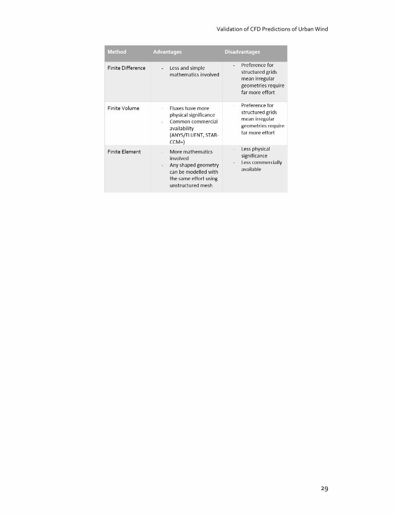
Validation of CFD Predictions of Urban Wind
29
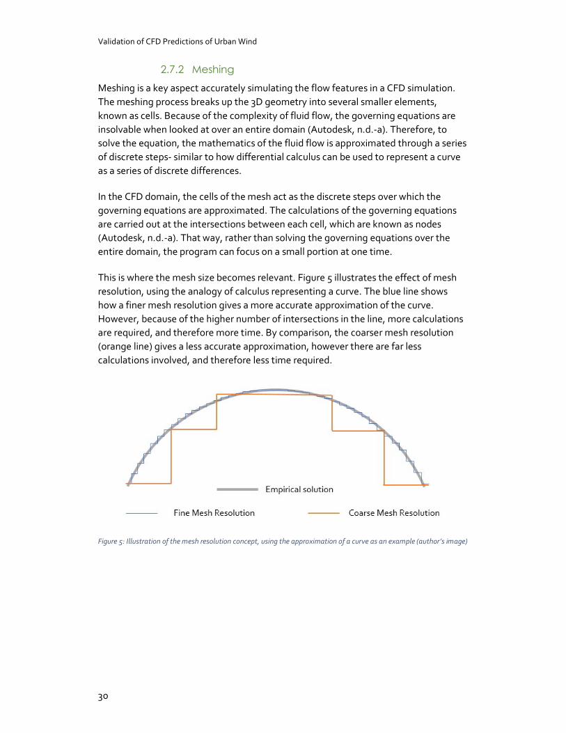
Validation of CFD Predictions of Urban Wind
30
2.7.2 Meshing
Meshing is a key aspect accurately simulating the flow features in a CFD simulation. The meshing process breaks up the 3D geometry into several smaller elements, known as cells. Because of the complexity of fluid flow, the governing equations are insolvable when looked at over an entire domain (Autodesk, n.d.-a). Therefore, to solve the equation, the mathematics of the fluid flow is approximated through a series of discrete steps- similar to how differential calculus can be used to represent a curve as a series of discrete differences.
In the CFD domain, the cells of the mesh act as the discrete steps over which the governing equations are approximated. The calculations of the governing equations are carried out at the intersections between each cell, which are known as nodes (Autodesk, n.d.-a). That way, rather than solving the governing equations over the entire domain, the program can focus on a small portion at one time.
This is where the mesh size becomes relevant. Figure 5 illustrates the effect of mesh resolution, using the analogy of calculus representing a curve. The blue line shows how a finer mesh resolution gives a more accurate approximation of the curve. However, because of the higher number of intersections in the line, more calculations are required, and therefore more time. By comparison, the coarser mesh resolution (orange line) gives a less accurate approximation, however there are far less calculations involved, and therefore less time required.
Figure 5: Illustration of the mesh resolution concept, using the approximation of a curve as an example (author’s image)
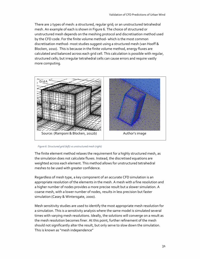
Validation of CFD Predictions of Urban Wind
31
There are 2 types of mesh: a structured, regular grid; or an unstructured tetrahedral mesh. An example of each is shown in Figure 6. The choice of structured or unstructured mesh depends on the meshing protocol and discretisation method used by the CFD code. For the finite volume method- which is the most common discretisation method- most studies suggest using a structured mesh (van Hooff & Blocken, 2010). This is because in the finite volume method, energy fluxes are calculated and balanced across each grid cell. This calculation is possible with regular, structured cells; but irregular tetrahedral cells can cause errors and require vastly more computing.
The finite element method relaxes the requirement for a highly structured mesh, as the simulation does not calculate fluxes. Instead, the discretised equations are weighted across each element. This method allows for unstructured tetrahedral meshes to be used with greater confidence.
Regardless of mesh type, a key component of an accurate CFD simulation is an appropriate resolution of the elements in the mesh. A mesh with a fine resolution and a higher number of nodes provides a more precise result but a slower simulation. A coarse mesh, with a lower number of nodes, results in less precision but faster simulation (Casey & Wintersgate, 2000).
Mesh sensitivity studies are used to identify the most appropriate mesh resolution for a simulation. This is a sensitivity analysis where the same model is simulated several times with varying mesh resolutions. Ideally, the solutions will converge on a result as the mesh resolution becomes finer. At this point, further refinement of the mesh should not significantly alter the result, but only serve to slow down the simulation. This is known as “mesh independence”
Source: (Ramponi & Blocken, 2012b)
Author’s image
Figure 6: Structured grid (left) vs unstructured mesh (right)

Validation of CFD Predictions of Urban Wind
32
2.7.3 Modelling Turbulence and the Simulation Process
The way that CFD models predict the effects of turbulence is an area which can significantly impact the accuracy of a simulation. Three different approaches are currently in common use for predicting turbulence: Direct Numerical Simulation (DNS), Large Eddy Simulation (LES), and Reynolds Averaged Navier-Stokes (RANS). The choice of regime determines the extent to which the governing equations of CFD are solved (Casey & Wintersgate, 2000; Franke, Hellsten, Schlunzen, & Carissimo, 2007).
For the complex flows encountered in urban environments, turbulent eddies around buildings range in scale from hundreds of metres long to fractions of a metre. It is possible to fully solve the governing equations for the turbulent eddies at all scales in a simulation: this is the DNS approach. However, the mesh size required to incorporate all of the eddy scales is tiny, and a huge number of node points are required (Murakami, 1998). This results in DNS requiring an impractical amount of time for even the most simple of CFD simulations (Franke et al., 2007).
RANS or LES approaches are used to circumvent the high computational and time requirements of the DNS method. Both the RANS and LES methods work by averaging the governing equations over a chosen quantity. The averaging process reduces the precision of the final simulation, while allowing a streamlined simulation process. Steady RANS equations are time averaged, while LES equations are spatially averaged (Blocken et al., 2010).
The time-averaged nature of RANS simulations mean that the simulation only predicts the mean flow, and does not explicitly predict any turbulent eddies. Instead, the effect of eddies on the average flow are predicted through turbulence models. There are a range of models, which cater to a variety of different CFD applications. The selection of an appropriate turbulence model for the analysis is an important aspect for accurate simulations.
Unlike RANS models, LES is not run on a time averaged basis. Therefore LES is closer to DNS, as it captures the flow at an instantaneous point, rather than simulating the mean flow features. Unlike DNS, LES utilises a user-defined filter to identify the scale of turbulent eddies to be fully realised. Any eddies that are smaller than the minimum filter size are approximated (Blocken et al., 2016). This significantly reduces the total number of calculations required, when compared to DNS simulation.
The averaging process employed by both RANS and LES models means that the mathematical model being solved have more unknowns than equations (Autodesk, n.d.-c). Therefore, the governing equations cannot be fully resolved in one simulation, so the simulation is resolved as an iterative process.
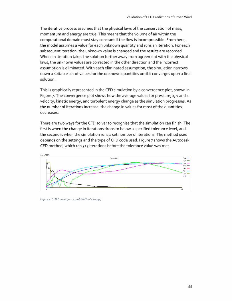
Validation of CFD Predictions of Urban Wind
33
The iterative process assumes that the physical laws of the conservation of mass, momentum and energy are true. This means that the volume of air within the computational domain must stay constant if the flow is incompressible. From here, the model assumes a value for each unknown quantity and runs an iteration. For each subsequent iteration, the unknown value is changed and the results are recorded. When an iteration takes the solution further away from agreement with the physical laws, the unknown values are corrected in the other direction and the incorrect assumption is eliminated. With each eliminated assumption, the simulation narrows down a suitable set of values for the unknown quantities until it converges upon a final solution.
This is graphically represented in the CFD simulation by a convergence plot, shown in Figure 7. The convergence plot shows how the average values for pressure; x, y and z velocity; kinetic energy, and turbulent energy change as the simulation progresses. As the number of iterations increase, the change in values for most of the quantities decreases.
There are two ways for the CFD solver to recognise that the simulation can finish. The first is when the change in iterations drops to below a specified tolerance level, and the second is when the simulation runs a set number of iterations. The method used depends on the settings and the type of CFD code used. Figure 7 shows the Autodesk CFD method, which ran 315 iterations before the tolerance value was met.
Figure 7: CFD Convergence plot (author's image)
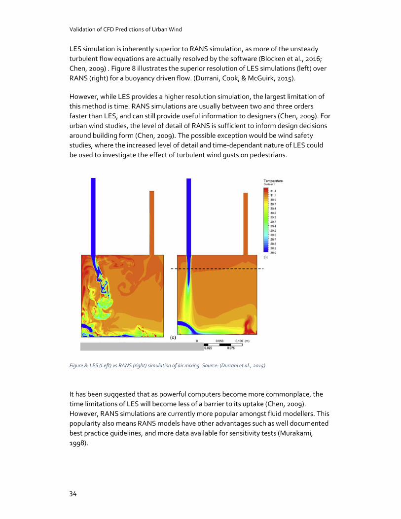
Validation of CFD Predictions of Urban Wind
34
LES simulation is inherently superior to RANS simulation, as more of the unsteady turbulent flow equations are actually resolved by the software (Blocken et al., 2016; Chen, 2009) . Figure 8 illustrates the superior resolution of LES simulations (left) over RANS (right) for a buoyancy driven flow. (Durrani, Cook, & McGuirk, 2015).
However, while LES provides a higher resolution simulation, the largest limitation of this method is time. RANS simulations are usually between two and three orders faster than LES, and can still provide useful information to designers (Chen, 2009). For urban wind studies, the level of detail of RANS is sufficient to inform design decisions around building form (Chen, 2009). The possible exception would be wind safety studies, where the increased level of detail and time-dependant nature of LES could be used to investigate the effect of turbulent wind gusts on pedestrians.
Figure 8: LES (Left) vs RANS (right) simulation of air mixing. Source: (Durrani et al., 2015)
It has been suggested that as powerful computers become more commonplace, the time limitations of LES will become less of a barrier to its uptake (Chen, 2009). However, RANS simulations are currently more popular amongst fluid modellers. This popularity also means RANS models have other advantages such as well documented best practice guidelines, and more data available for sensitivity tests (Murakami, 1998).
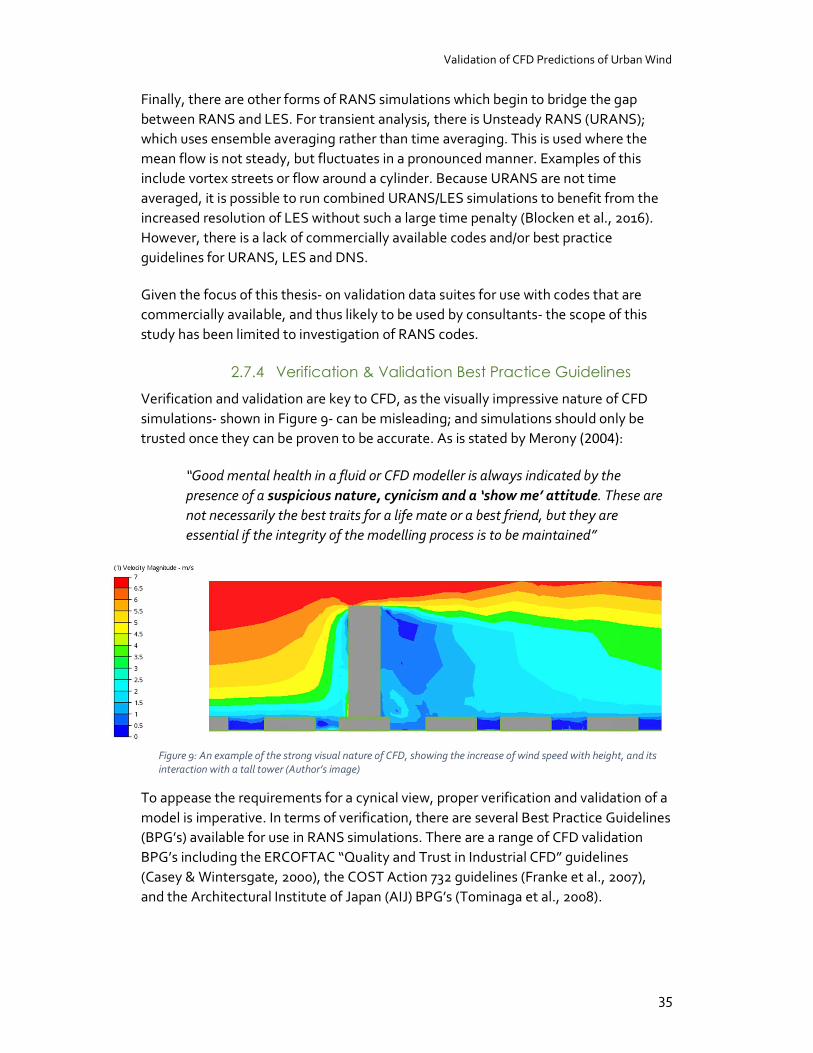
Validation of CFD Predictions of Urban Wind
35
Finally, there are other forms of RANS simulations which begin to bridge the gap between RANS and LES. For transient analysis, there is Unsteady RANS (URANS); which uses ensemble averaging rather than time averaging. This is used where the mean flow is not steady, but fluctuates in a pronounced manner. Examples of this include vortex streets or flow around a cylinder. Because URANS are not time averaged, it is possible to run combined URANS/LES simulations to benefit from the increased resolution of LES without such a large time penalty (Blocken et al., 2016). However, there is a lack of commercially available codes and/or best practice guidelines for URANS, LES and DNS.
Given the focus of this thesis- on validation data suites for use with codes that are commercially available, and thus likely to be used by consultants- the scope of this study has been limited to investigation of RANS codes.
2.7.4 Verification & Validation Best Practice Guidelines
Verification and validation are key to CFD, as the visually impressive nature of CFD simulations- shown in Figure 9- can be misleading; and simulations should only be trusted once they can be proven to be accurate. As is stated by Merony (2004):
“Good mental health in a fluid or CFD modeller is always indicated by the presence of a suspicious nature, cynicism and a ‘show me’ attitude. These are not necessarily the best traits for a life mate or a best friend, but they are essential if the integrity of the modelling process is to be maintained”
Figure 9: An example of the strong visual nature of CFD, showing the increase of wind speed with height, and its interaction with a tall tower (Author’s image)
To appease the requirements for a cynical view, proper verification and validation of a model is imperative. In terms of verification, there are several Best Practice Guidelines (BPG’s) available for use in RANS simulations. There are a range of CFD validation BPG’s including the ERCOFTAC “Quality and Trust in Industrial CFD” guidelines (Casey & Wintersgate, 2000), the COST Action 732 guidelines (Franke et al., 2007), and the Architectural Institute of Japan (AIJ) BPG’s (Tominaga et al., 2008).
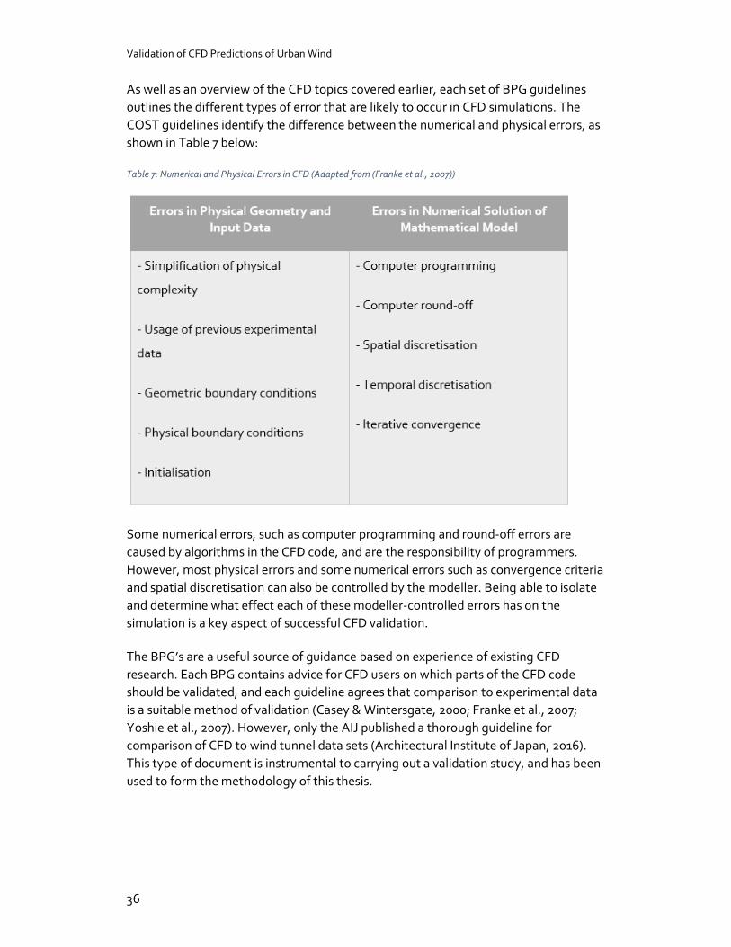
Validation of CFD Predictions of Urban Wind
36
As well as an overview of the CFD topics covered earlier, each set of BPG guidelines outlines the different types of error that are likely to occur in CFD simulations. The COST guidelines identify the difference between the numerical and physical errors, as shown in Table 7 below:
Table 7: Numerical and Physical Errors in CFD (Adapted from (Franke et al., 2007))
Some numerical errors, such as computer programming and round-off errors are caused by algorithms in the CFD code, and are the responsibility of programmers. However, most physical errors and some numerical errors such as convergence criteria and spatial discretisation can also be controlled by the modeller. Being able to isolate and determine what effect each of these modeller-controlled errors has on the simulation is a key aspect of successful CFD validation.
The BPG’s are a useful source of guidance based on experience of existing CFD research. Each BPG contains advice for CFD users on which parts of the CFD code should be validated, and each guideline agrees that comparison to experimental data is a suitable method of validation (Casey & Wintersgate, 2000; Franke et al., 2007; Yoshie et al., 2007). However, only the AIJ published a thorough guideline for comparison of CFD to wind tunnel data sets (Architectural Institute of Japan, 2016). This type of document is instrumental to carrying out a validation study, and has been used to form the methodology of this thesis.

Validation of CFD Predictions of Urban Wind
37
Wind tunnel and Small Scale modelling
The literature on small scale modelling of the wind effects of buildings shows that trustworthiness is not only a key consideration for CFD simulations. For wind tunnel modelling, considerable effort was put into validating the approach flow and wind speed/pressure results as the ability to recreate atmospheric conditions at small scales was refined. By the 1960’s, the process had shown itself to be trustworthy enough for use in engineering applications, with the World Trade Center in New York being one of the first to be designed using this technique (Cochran & Derickson, 2011). Currently, wind tunnel tests are seen as the most accurate method of predicting wind effects on buildings, even more so than full-scale measurements (Carpenter, 2002; Shilston, 2015).
Currently, the Wellington City Council (WCC) requires a wind tunnel test or wind assessment for all proposed new buildings over 18.6m tall. The objective of these assessments is to identify the effect of the new building on the both the safety and comfort of pedestrians. To prove the trustworthiness of the analysis, the wind tunnel test must contain a calibration section which identifies the flow visualisations of a single isolated building (Wellington City Council, 2014a).

Validation of CFD Predictions of Urban Wind
38
2.8.1 Wind Tunnel Measurement techniques
For calibration and validation of CFD, the measurement method of wind speeds in the wind tunnel is a key consideration. The method used to measure the wind tunnel data determines the level of detail provided to calibrate CFD data against. It also provides a variety of different measurable variables to compare the CFD analysis against.
There are two groups of wind tunnel tests:
- Tests which collect qualitative data. - Tests which collect quantitative data.
The qualitative data studies provide visualisation of the overall flow, while the quantitative data provides detailed information relating to wind speeds in particular areas. While both can be useful to assessing the trustworthiness of CFD, only quantitative data has the necessary level of detail for validation.
Examples of qualitative studies include flow visualisation techniques, such as smoke (as used by Pendwarden & Wise, 1975), or flags. Other types include erosion techniques, which use lightweight materials such as sand, bran, polystyrene or cork particles (Carpenter, 2002; Davies, 1992). By looking at the pattern of erosion of these particles by the wind flow, it is possible to identify where areas of high wind speed will occur. The strength of this technique is identifying problem areas where further wind speed measurements should be undertaken. However, this technique cannot provide measured wind speeds, so must be used in conjunction with quantitative measurements.
There are several techniques for collecting quantitative wind speed data. These include Irwin probes, hot film or hot wire anemometers, split film probes, or laser-Doppler anemometry (Blocken, 2014; Blocken et al., 2016; Karava, 2008). Particle Image velocimetry (PIV) is another technique which provides 2-Dimensional visualisations and data on the flow over a large part of the area under study. The data is measured in 2 dimensions, meaning the results are recorded as vectors (Karava, 2008). Of the two validation sets that provided data, hot film anemometers and split fibre anemometers were used to measure wind speeds. For the sake of brevity and relevance, only those two wind measurement techniques are investigated.
Validation of CFD Predictions of Urban Wind
39
2.8.2 How Ohms law is used to estimate wind speeds
Both split film and hot wire anemometry use the principle of Ohm’s law to measure wind speed in wind tunnels. Ohm’s law states that a current through an electrical component with a constant resistance is directly proportional to the voltage across that component. Therefore, assuming a constant voltage, the current and resistance through the component are inversely proportional.
Hot film and hot wire anemometers exploit this relationship to measure wind speed. The probes which measure wind speed consist of a very fine film of metal, which is placed over a non-conducting ceramic or quartz-cylinder sensor (Jorgenson, 2002). A current is then run through the film, which causes it to heat up to well above the ambient air temperature. Because of this, the metals selected to make the film have a high coefficient of resistance, such as tungsten or platinum. When these probes are placed in a wind tunnel, the air flow past the probes exerts a cooling effect (Blocken et al., 2016).
The way that the cooling effect is used depends whether the probes are set up for Constant Current Anemometry (CCA), Constant Voltage Anemometry (CVA), or Constant Temperature Anemometry (CTA). As the names suggest, each type of anemometry works by trying to maintaining a constant variable, either current, voltage, or temperature. The output from the probes come in the form of the varying voltages throughout the test. The relationship between each variable and the resistance of the wire is then used to obtain an estimate of the flow speed (Blocken et al., 2016).
2.8.3 Split film anemometry
The AIJ dataset utilised a split fibre probe which measured the velocity in 3 directions: x, y and z (Architectural Institute of Japan, 2016). Split fibre probes are not used as extensively in pedestrian level wind studies as other methods such as hot wire and hot film anemometry. The cost of split film probes can be a limiting factor for their use, as can the fact that they are not always supported by standard constant temperature anemometer software (Jorgenson, 2002).
However, the probes respond to both the magnitude and direction of the velocity vector, information about both can be obtained (Albrecht, 2003). This provides a highly in-depth level of data which can be used to validate CFD simulations.
2.8.4 Hot film anemometry
Data from the Standard City set was measured using a hot film anemometer. Hot film anemometry is omnidirectional, which means that only the magnitude of the wind speed can be calculated. Omnidirectional probes are also affected by the direction that they are placed in the wind tunnel. The Probes placed in the standard city were vertical, meaning that they picked up the wind as it passed the probe in the

Validation of CFD Predictions of Urban Wind
40
perpendicular horizontal plane. Any fluctuations in the wind direction are expressed as part of the overall velocity magnitude. Because of this, high levels of turbulence can adversely affect the accuracy of the probe (Jorgenson, 2002).
All probe types must be calibrated, to test that the response of the film reflects the governing relationship to Ohm’s law. However, for multi-axial probes- such as split film probes- calibration must be carried out in 3 directions (Albrecht, 2003; Jorgenson, 2002). This makes calibration of these probes more time-consuming and arduous, and can be considered a benefit of the more low-maintenance hot film anemometers.
2.8.5 Information required for CFD validation
To ensure that the CFD modelling process is capable of recreating realistic wind flow conditions, it is important that the variation of both wind speed and turbulence with height can be represented as a flow into the CFD digital wind tunnel. The way that wind flow and turbulence is represented by the CFD model should match the way that these conditions are represented in the physical wind tunnel, which in turn should be ensured to be a reasonably accurate representation of reality.
Several mathematical models are used to represent the relationship between wind speed, turbulence and height. One method is a power law, as described by (Gandemer, 1975). Similarly, Deaves and Harris (1978) developed a mathematical relationship which was shown to accurately represent the relationship between height, turbulence and wind speed. Recreating these mathematical models provides confidence that the wind profile in the wind tunnel is an accurate representation of reality.
To ensure that the CFD model reflects this relationship, the inlet profiles for wind speed and turbulence are an important requirement of a CFD validation set. Without the ability to accurately model the inlet flow, it is not possible to compare whether a CFD model accurately simulates the flow generated in a wind tunnel.
Similarly, it is common practice both in CFD and wind tunnel tests to normalise the wind speed at pedestrian level against the wind speed at free flow conditions. Typically, this is a wind speed measurement taken at 100m or 150m scale height above the configuration (Carpenter, 2002). The measured wind speeds are then represented as a ratio of this free flow velocity. Expressing the data as a ratio is preferable to expressing the results as absolute velocities as it reduces the overall variation, and shows the relationship between points more clearly. It also allows wind tunnel results to be extrapolated throughout the year via comparison to meteorological data. This is useful for planners, who wish to make design decisions based on the effects of a design throughout the entire year, rather than for a single snapshot.
Validation of CFD Predictions of Urban Wind
41
3. The CFD Validation Process
The assessment of existing wind tunnel tests for generic configurations carried out in Section 2.3 found that only two of the 29 sets identified are viable for CFD validation of urban flows, mostly due to the lack of available data. Of the two sets, the AIJ set is specifically suited to validating CFD analyses. However, the Standard City data set has more configurations, which makes it better for recreating the flow features that are likely to be found in an actual city.
The goal of creating a validation suite is to produce a tool that could be used by the Wellington City Council to measure the trustworthiness of CFD simulations. There are two steps to this: firstly, to identify a suitable model or set of models for this assessment. This was the purpose of Chapter 2. The second step was to determine whether these models can be applied as a validation dataset to a CFD program. To do this, the validation method described by Blocken, Janssen, & van Hooff (2012) was used to identify the trustworthiness of a single CFD code for simulating urban wind flow, as a test case of the validation process. This chapter reports the selection of the validation type, CFD code, comparison process, and accuracy criteria to provide a robust methodology test.
Validation of CFD Predictions of Urban Wind
42
The best validation method is through comparison to wind tunnel measurements
3.1.1 The BESTEST definition of validation
The principles of validation for building energy simulation (BES) software were outlined as part of the Building Energy Simulation Test (BESTEST) (Judkoff, Wortman, O’Doherty, & Burch, 2008). Although BESTEST was designed as a method of validating building energy models, the basic principles of the validation process still hold true for CFD simulations.
The BESTEST documentation defines three types of validation study that are necessary for full validation of building energy simulation software. The BESTEST authors recommend that for a robust validation more than one of these approaches should be undertaken (Judkoff et al., 2008). The three are: Analytical studies, Comparative studies, and Empirical studies. The BESTEST was designed so that each type of verification study is necessary for the validation process as a whole (Judkoff et al., 2008).
- Analytical Studies
The first of the three validation types are Analytical studies. These are effectively a comparison of modelling software against the governing equations, for an extreme case where all the variables are controlled. The BESTEST examples involve isolating individual building elements, and testing the heat flow through them. Because the heat flow through these elements was in one direction only, enough parameters were controlled that the software calculations can be solved with hand calculations. These act as the truth model for this type of verification (Judkoff et al., 2008).
As with thermal simulations, the governing equations of CFD are highly complex, which limits the analytical solutions to very simple geometries with well-defined fluid properties. Often in real world engineering applications, these conditions do not exist, resulting in the requirement for physical testing (Cochran & Derickson, 2011). Therefore, analytical validation against hand calculations is not a viable method for CFD models.
- Comparative Studies
Comparative studies consist of finding consensus between several models of the same physical phenomenon. The main benefit of this method is that no measured or calculated data is required. However, due to the lack of measured data, comparative studies also lack a “truth test”, which means that either analytical or empirical validation must also be carried out before the results can be deemed trustworthy (Judkoff et al., 2008). Examples of comparative studies in CFD modelling include
Validation of CFD Predictions of Urban Wind
43
validation against other CFD code results, or against small scale models such as salt bath or wind tunnel models (Architectural Institute of Japan, 2016).
- Empirical Studies
Empirical studies consist of comparing a simulation against measured data. Empirical studies are as trustworthy as the measured data; therefore, the measurements must be taken carefully to reduce errors. It is also important that the measured data is at a sufficient level of detail for comparison to simulated results. This allows detailed, reliable conclusions to be drawn based on data which is representative of the situation being explored.
The drawbacks of empirical studies are the high cost and time consuming nature of setting up the measurement equipment. An example of experimental validation was carried out in Japan in 1978. Wind speeds around a site were measured for 4 years, before and after the construction of a high-rise building (Murakami et al., 1978) . These results were later used in conjunction with wind tunnel tests to validate a CFD analysis of the same site. The time requirements for empirical validation are the largest barrier to Empirical validation within the 1 year scope of a Master’s thesis.
3.1.2 What is the BESTEST validation test for CFD?
When choosing which validation test is the most appropriate for CFD analyses, it is important to consider the aim of each validation method. Validation can focus on one of two areas:
- Numerical diffusion: whether the mathematical algorithms which analyse the governing equations are accurate. This type of error would be identified using analytical validation.
- Physical Diffusion: whether the model and its settings are appropriate for the case under investigation. This type of diffusion would be identified by comparative or empirical validation.
The target audience of this thesis is building designers and engineers, not CFD code writers. Therefore, the focus is to find the best method of validating CFD simulation with regards to physical diffusion. This means that an in-depth investigation of the algorithms used in a CFD analysis is outside of the scope of any validation work to be carried out.
Analytical validation is not a suitable method, as it deals exclusively with the algorithms. Additionally, the purpose of validation in this case is to trust CFD simulations of complex urban environments. A simple test case, as required by the analytical method, would not be relevant to this type of test.
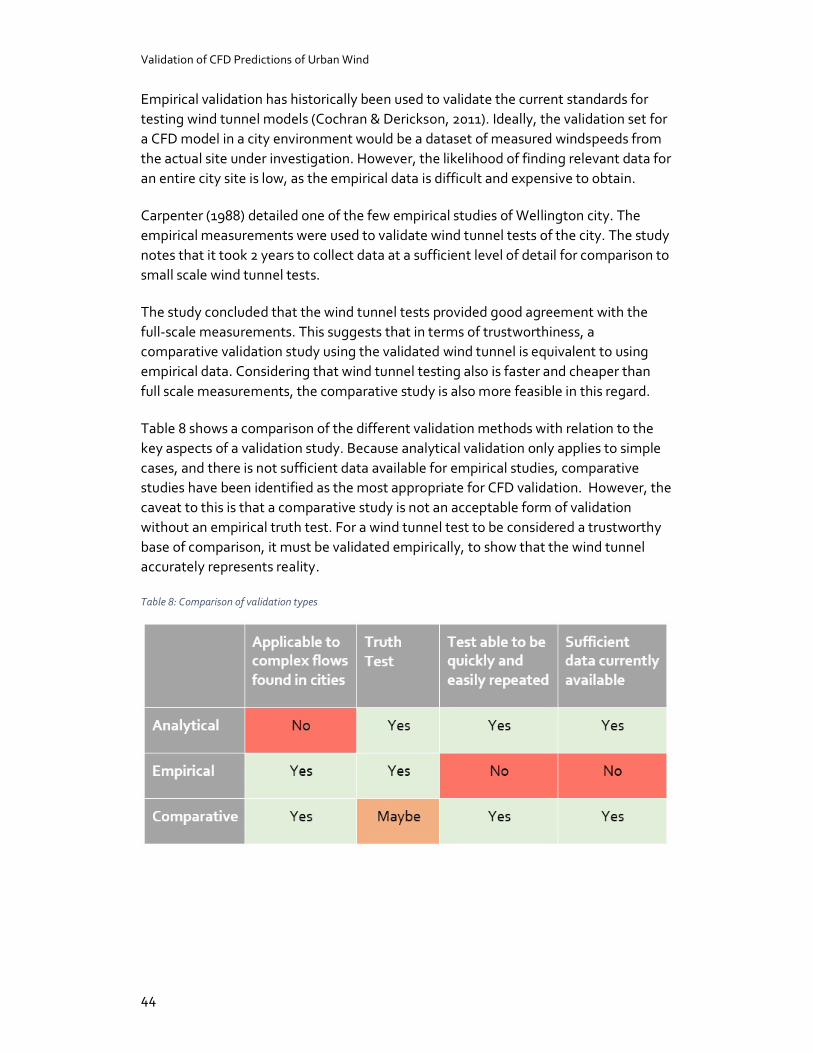
Validation of CFD Predictions of Urban Wind
44
Empirical validation has historically been used to validate the current standards for testing wind tunnel models (Cochran & Derickson, 2011). Ideally, the validation set for a CFD model in a city environment would be a dataset of measured windspeeds from the actual site under investigation. However, the likelihood of finding relevant data for an entire city site is low, as the empirical data is difficult and expensive to obtain.
Carpenter (1988) detailed one of the few empirical studies of Wellington city. The empirical measurements were used to validate wind tunnel tests of the city. The study notes that it took 2 years to collect data at a sufficient level of detail for comparison to small scale wind tunnel tests.
The study concluded that the wind tunnel tests provided good agreement with the full-scale measurements. This suggests that in terms of trustworthiness, a comparative validation study using the validated wind tunnel is equivalent to using empirical data. Considering that wind tunnel testing also is faster and cheaper than full scale measurements, the comparative study is also more feasible in this regard.
Table 8 shows a comparison of the different validation methods with relation to the key aspects of a validation study. Because analytical validation only applies to simple cases, and there is not sufficient data available for empirical studies, comparative studies have been identified as the most appropriate for CFD validation. However, the caveat to this is that a comparative study is not an acceptable form of validation without an empirical truth test. For a wind tunnel test to be considered a trustworthy base of comparison, it must be validated empirically, to show that the wind tunnel accurately represents reality.
Table 8: Comparison of validation types
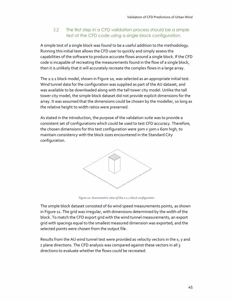
Validation of CFD Predictions of Urban Wind
45
The first step in a CFD validation process should be a simple test of the CFD code using a single block configuration.
A simple test of a single block was found to be a useful addition to the methodology. Running this initial test allows the CFD user to quickly and simply assess the capabilities of the software to produce accurate flows around a single block. If the CFD code is incapable of recreating the measurements found in the flow of a single block, then it is unlikely that it will accurately recreate the complex flows in a large array.
The 2:1:1 block model, shown in Figure 10, was selected as an appropriate initial test. Wind tunnel data for the configuration was supplied as part of the AIJ dataset, and was available to be downloaded along with the tall tower city model. Unlike the tall tower city model, the simple block dataset did not provide explicit dimensions for the array. It was assumed that the dimensions could be chosen by the modeller, so long as the relative height to width ratios were preserved.
As stated in the introduction, the purpose of the validation suite was to provide a consistent set of configurations which could be used to test CFD accuracy. Therefore, the chosen dimensions for this test configuration were 30m x 30m x 60m high, to maintain consistency with the block sizes encountered in the Standard City configuration.
Figure 10: Axonometric view of the 2:1:1 block configuraton
The simple block dataset consisted of 60 wind speed measurements points, as shown in Figure 11. The grid was irregular, with dimensions determined by the width of the block. To match the CFD export grid with the wind tunnel measurements, an export grid with spacings equal to the smallest measured dimension was exported, and the selected points were chosen from the output file.
Results from the AIJ wind tunnel test were provided as velocity vectors in the x, y and z plane directions. The CFD analysis was compared against these vectors in all 3 directions to evaluate whether the flows could be recreated.
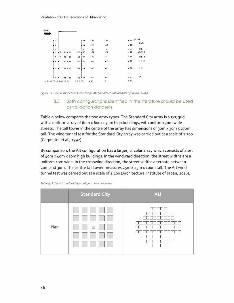
Validation of CFD Predictions of Urban Wind
46
Figure 11: Simple Block Measurement points (Architectural Institute of Japan, 2016).
Both configurations identified in the literature should be used as validation datasets
Table 9 below compares the two array types. The Standard City array is a 5x5 grid, with a uniform array of 60m x 60m x 30m high buildings, with uniform 30m wide streets. The tall tower in the centre of the array has dimensions of 30m x 30m x 270m tall. The wind tunnel test for the Standard City array was carried out at a scale of 1:300 (Carpenter et al., 1992).
By comparison, the AIJ configuration has a larger, circular array which consists of a set of 40m x 40m x 10m high buildings. In the windward direction, the street widths are a uniform 10m wide. In the crosswind direction, the street widths alternate between 20m and 30m. The centre tall tower measures 25m x 25m x 100m tall. The AIJ wind tunnel test was carried out at a scale of 1:400 (Architectural Institute of Japan, 2016).
Table 9: AIJ and Standard City configuration comparison
Standard City AIJ
Plan
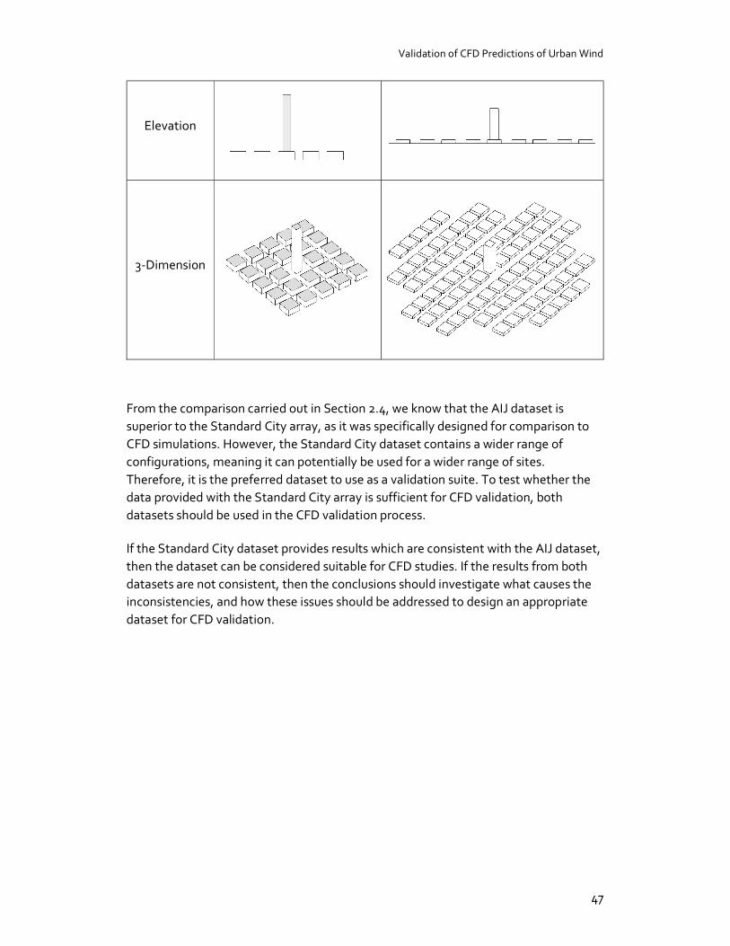
Validation of CFD Predictions of Urban Wind
47
Elevation
3-Dimension
From the comparison carried out in Section 2.4, we know that the AIJ dataset is superior to the Standard City array, as it was specifically designed for comparison to CFD simulations. However, the Standard City dataset contains a wider range of configurations, meaning it can potentially be used for a wider range of sites. Therefore, it is the preferred dataset to use as a validation suite. To test whether the data provided with the Standard City array is sufficient for CFD validation, both datasets should be used in the CFD validation process.
If the Standard City dataset provides results which are consistent with the AIJ dataset, then the dataset can be considered suitable for CFD studies. If the results from both datasets are not consistent, then the conclusions should investigate what causes the inconsistencies, and how these issues should be addressed to design an appropriate dataset for CFD validation.
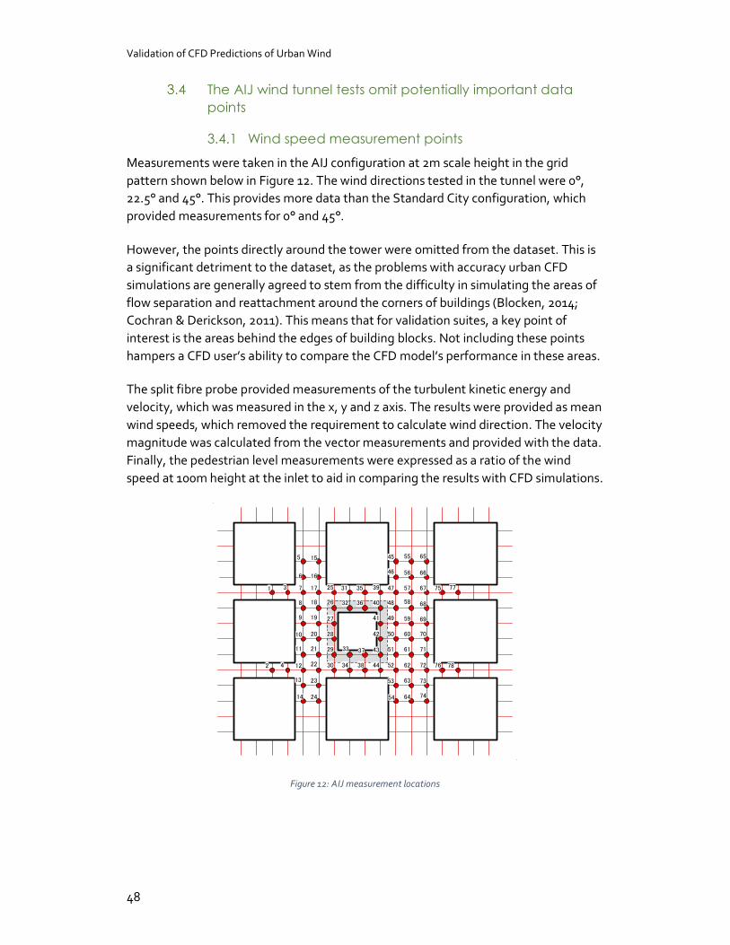
Validation of CFD Predictions of Urban Wind
48
The AIJ wind tunnel tests omit potentially important data points
3.4.1 Wind speed measurement points
Measurements were taken in the AIJ configuration at 2m scale height in the grid pattern shown below in Figure 12. The wind directions tested in the tunnel were 0°, 22.5° and 45°. This provides more data than the Standard City configuration, which provided measurements for 0° and 45°.
However, the points directly around the tower were omitted from the dataset. This is a significant detriment to the dataset, as the problems with accuracy urban CFD simulations are generally agreed to stem from the difficulty in simulating the areas of flow separation and reattachment around the corners of buildings (Blocken, 2014; Cochran & Derickson, 2011). This means that for validation suites, a key point of interest is the areas behind the edges of building blocks. Not including these points hampers a CFD user’s ability to compare the CFD model’s performance in these areas.
The split fibre probe provided measurements of the turbulent kinetic energy and velocity, which was measured in the x, y and z axis. The results were provided as mean wind speeds, which removed the requirement to calculate wind direction. The velocity magnitude was calculated from the vector measurements and provided with the data. Finally, the pedestrian level measurements were expressed as a ratio of the wind speed at 100m height at the inlet to aid in comparing the results with CFD simulations.
Figure 12: AIJ measurement locations
1
2
3
4
5
6
7
8
9
10
11
12
13
14
15
16
17
18
19
20
21
22
23
24
25
26
27
28
29
30
31
32
33
34
35
36
37
38
39
40
41
42
43
44
45
46
47
48
49
50
51
52
53
54
55
56
57
58
59
60
61
62
63
64
65
66
67
68
69
70
71
72
73
74
75
76
77
78
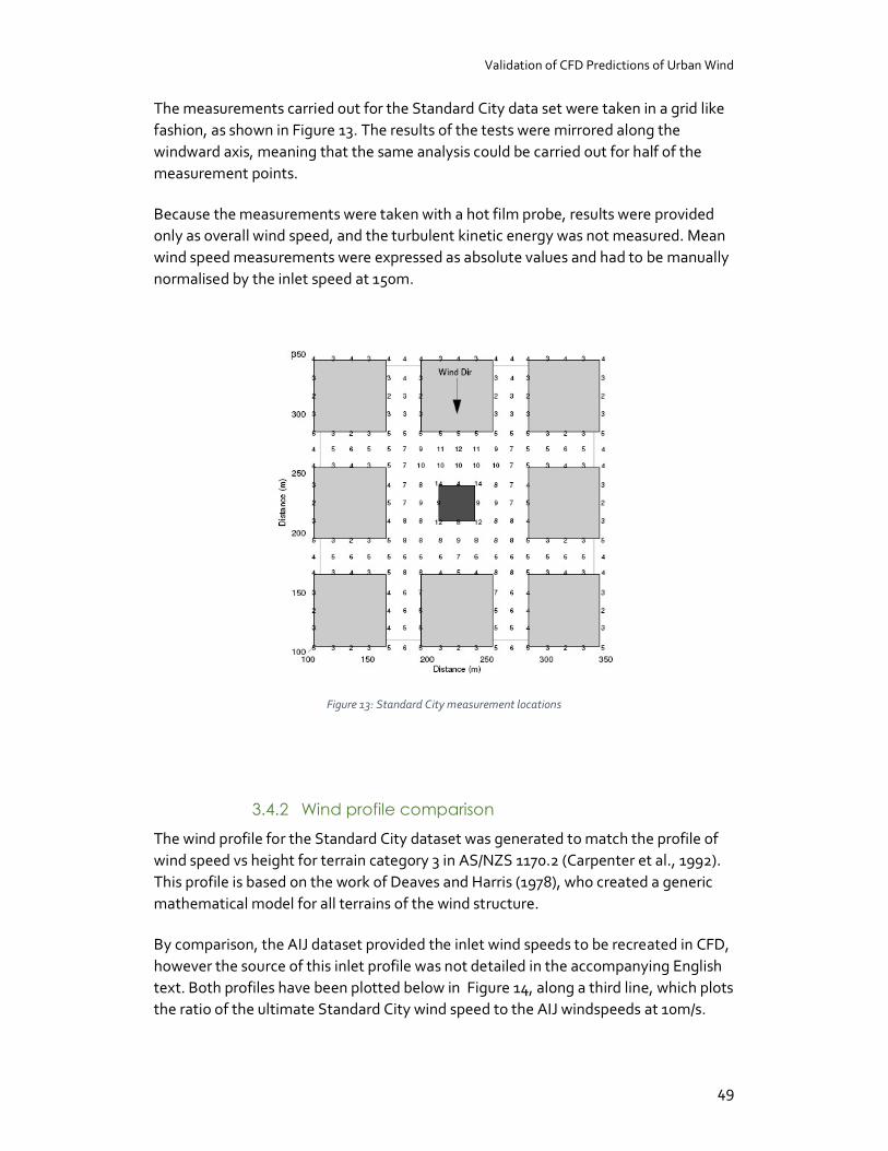
Validation of CFD Predictions of Urban Wind
49
The measurements carried out for the Standard City data set were taken in a grid like fashion, as shown in Figure 13. The results of the tests were mirrored along the windward axis, meaning that the same analysis could be carried out for half of the measurement points.
Because the measurements were taken with a hot film probe, results were provided only as overall wind speed, and the turbulent kinetic energy was not measured. Mean wind speed measurements were expressed as absolute values and had to be manually normalised by the inlet speed at 150m.
Figure 13: Standard City measurement locations
3.4.2 Wind profile comparison
The wind profile for the Standard City dataset was generated to match the profile of wind speed vs height for terrain category 3 in AS/NZS 1170.2 (Carpenter et al., 1992). This profile is based on the work of Deaves and Harris (1978), who created a generic mathematical model for all terrains of the wind structure.
By comparison, the AIJ dataset provided the inlet wind speeds to be recreated in CFD, however the source of this inlet profile was not detailed in the accompanying English text. Both profiles have been plotted below in Figure 14, along a third line, which plots the ratio of the ultimate Standard City wind speed to the AIJ windspeeds at 10m/s.
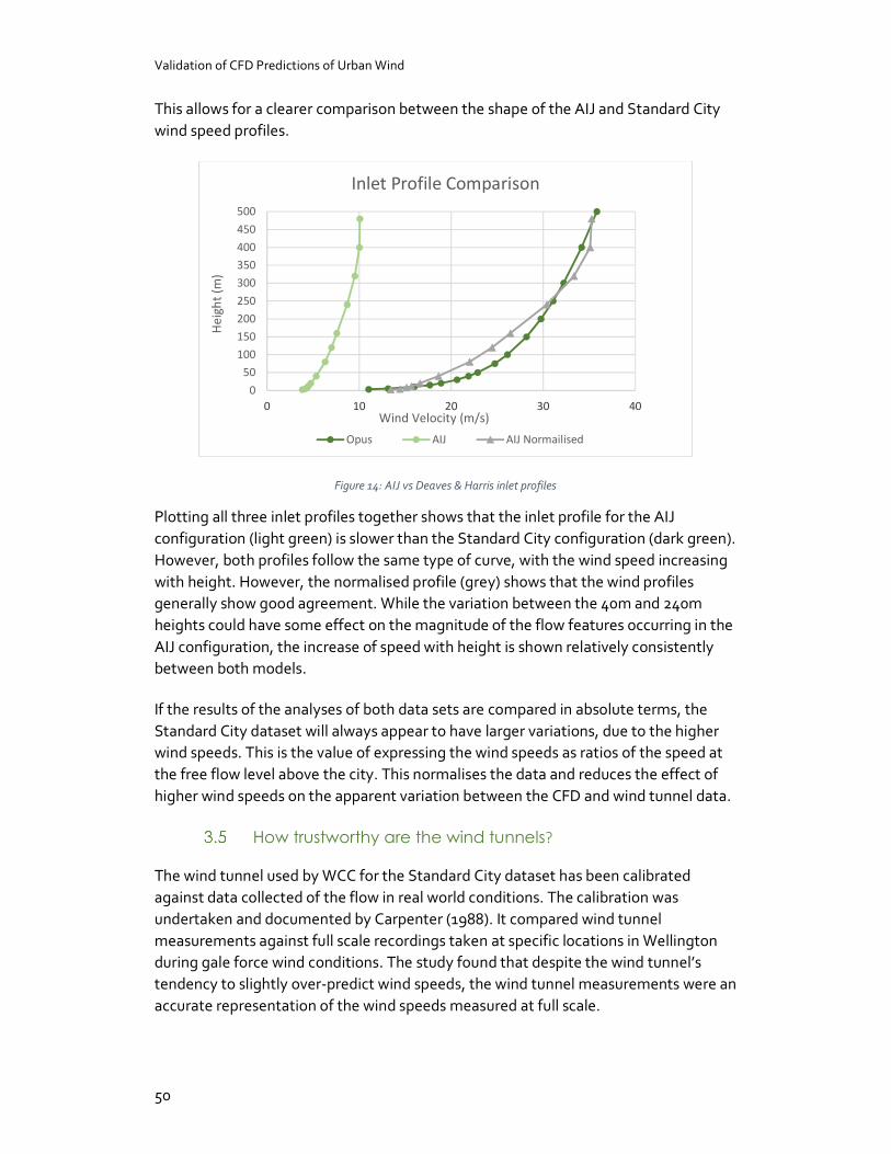
Validation of CFD Predictions of Urban Wind
50
This allows for a clearer comparison between the shape of the AIJ and Standard City wind speed profiles.
Figure 14: AIJ vs Deaves & Harris inlet profiles
Plotting all three inlet profiles together shows that the inlet profile for the AIJ configuration (light green) is slower than the Standard City configuration (dark green). However, both profiles follow the same type of curve, with the wind speed increasing with height. However, the normalised profile (grey) shows that the wind profiles generally show good agreement. While the variation between the 40m and 240m heights could have some effect on the magnitude of the flow features occurring in the AIJ configuration, the increase of speed with height is shown relatively consistently between both models.
If the results of the analyses of both data sets are compared in absolute terms, the Standard City dataset will always appear to have larger variations, due to the higher wind speeds. This is the value of expressing the wind speeds as ratios of the speed at the free flow level above the city. This normalises the data and reduces the effect of higher wind speeds on the apparent variation between the CFD and wind tunnel data.
How trustworthy are the wind tunnels?
The wind tunnel used by WCC for the Standard City dataset has been calibrated against data collected of the flow in real world conditions. The calibration was undertaken and documented by Carpenter (1988). It compared wind tunnel measurements against full scale recordings taken at specific locations in Wellington during gale force wind conditions. The study found that despite the wind tunnel’s tendency to slightly over-predict wind speeds, the wind tunnel measurements were an accurate representation of the wind speeds measured at full scale.
050
100150200250300350400450500
0 10 20 30 40
Hei
ght (
m)
Wind Velocity (m/s)
Inlet Profile Comparison
Opus AIJ AIJ Normailised

Validation of CFD Predictions of Urban Wind
51
While the English AIJ documentation did not contain any evidence of a similar trustworthiness exercise, personal correspondence with a Japanese academic revealed that the AIJ published a Japanese document set detailing a similar validation exercise of the wind tunnel measurements (Sakai, 2017). Using wind tunnel measurements that have been validated against empirical measurements, allows the comparative validation study to overcome the “truth test” limitation, as the wind tunnel measurements can then be considered representative of real flows.
Autodesk CFD is the Most Appropriate code for the validation
There are a large number of both open-source and commercial CFD codes available. To aid in the selection of an appropriate code, a set of criteria was developed. These criteria were informed by past studies using CFD in urban contexts, and centred on a balance between the usability, robustness, and availability of each CFD program. The following is a consideration of each criteria, along with a description of why each is important.
What is the availability of each code to Victoria University of Wellington?
It is likely that if a code is difficult to procure within the university, it will be similarly difficult to obtain within the construction industry within New Zealand. Therefore, if a CFD code was not available for use at the university it was discounted from selection.
Is it possible to edit geometry within the software? Can geometry easily be imported from a range of exterior programs?
A highly desirable criterion was the ability to import and translate the geometry from a 3D modelling program which is readily available to the construction industry. The geometry was created using Autodesk Revit, as this is an example of a readily available 3D modelling program. The tool’s flexibility with creating and importing geometry was considered, and a higher rating was given for a smooth import process with the fewest iterations and file conversions.
Is the CFD code designed for the simulation of flows around buildings?
Some CFD codes are tailored towards simulating airflow around buildings, while others are used for a range of situations. This category is focussed on the ability of the modeller to input conditions such as the wind inlet profile, appropriate boundary conditions for pedestrian wind studies, and reporting the appropriate results.
Validation of CFD Predictions of Urban Wind
52
Are there any documented cases of validation for each CFD code? Is the validation relevant to wind flows in urban areas?
This thesis tests a validation method, so any existing validation data serves as a useful base of comparison.
Does the program have a well-documented and freely available learning support structure? Is this learning support easily understandable and relevant to CFD simulations for urban wind flows? Is there a Q&A type forum set up to aid users for specific issues?
To be sure that the validation tests were running correctly, it was important for consultants to be able to quickly learn how to run the program and set up robust simulations. Therefore, this was one of the most important considerations when choosing the CFD code. The ability to self-learn and quickly solve any issues with the simulation was a key consideration. Codes were scored higher when they contained a well referenced help file, or forum with the ability to contact CFD experts.
Is the user face intuitive and easy to learn? Similarly, does the program allow the flexibility required to format and export data in a useful manner?
Similar to the above criteria, this was a focus because the aim was not to spend more time than necessary learning the graphical interface. Codes were scored highly when the layout and interface made the software more intuitive to use.
Exporting Results
Because of how variable wind speeds can be depending on location, the ability to accurately select points to export results from is another important consideration. With both sets of wind tunnel data supplying measurements in a grid layout, a higher rating was given to codes that could easily recreate the grid layout.
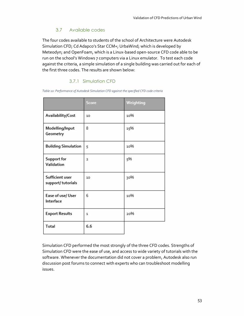
Validation of CFD Predictions of Urban Wind
53
Available codes
The four codes available to students of the school of Architecture were Autodesk Simulation CFD; Cd Adapco’s Star CCM+; UrbaWind; which is developed by Meteodyn; and OpenFoam, which is a Linux-based open-source CFD code able to be run on the school’s Windows 7 computers via a Linux emulator. To test each code against the criteria, a simple simulation of a single building was carried out for each of the first three codes. The results are shown below:
3.7.1 Simulation CFD
Table 10: Performance of Autodesk Simulation CFD against the specified CFD code criteria
Simulation CFD performed the most strongly of the three CFD codes. Strengths of Simulation CFD were the ease of use, and access to wide variety of tutorials with the software. Whenever the documentation did not cover a problem, Autodesk also run discussion post forums to connect with experts who can troubleshoot modelling issues.

Validation of CFD Predictions of Urban Wind
54
Simulation CFD is the only selected CFD code which uses the finite element method for discretisation. While commercial CFD codes which use the finite element method are not common, the best practice guidelines state that the advice provided is just as applicable to the finite element method as to the other, more common methods (Casey & Wintersgate, 2000).
Simulation CFD was specifically designed to import geometry from Autodesk programs such as Revit. This is useful as it requires less geometry conversions between a building model and the CFD analysis. However, a drawback of the Simulation CFD workflow is that the software does not allow users to edit the 3D geometry within the program. This means that if there are any problems with the geometry, the whole workflow must be restarted from the modelling software stage.
While Simulation CFD is not specifically designed for modelling buildings, the software is designed to be flexible for many CFD applications. There are a set of guidelines on CFD modelling for external flows, which were used to guide the initial test runs, and worked well.
The largest weakness with Simulation CFD was the process of exporting results. In the program, results were shown on isometric results planes. However, the only method of exporting wind speed results was as a uniform grid across the entire place. The modeller cannot independently control the location of the grid, but can control the resolution. This means that the alignment of the export grid with the wind tunnel measurements was controlled by re-locating the geometry until the grid locations lined up closely with the measurements.
Not being able to resize the grid also meant that data was exported for the entire domain, rather than the area of interest. This made post-processing of the data into a laborious task. While Simulation CFD has been validated for a range of applications, there is no evidence of its validation for external flows.
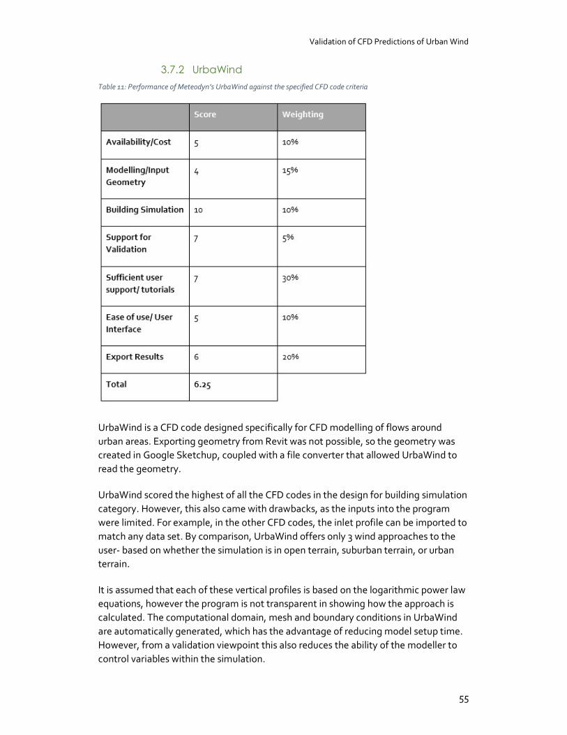
Validation of CFD Predictions of Urban Wind
55
3.7.2 UrbaWind
Table 11: Performance of Meteodyn’s UrbaWind against the specified CFD code criteria
UrbaWind is a CFD code designed specifically for CFD modelling of flows around urban areas. Exporting geometry from Revit was not possible, so the geometry was created in Google Sketchup, coupled with a file converter that allowed UrbaWind to read the geometry.
UrbaWind scored the highest of all the CFD codes in the design for building simulation category. However, this also came with drawbacks, as the inputs into the program were limited. For example, in the other CFD codes, the inlet profile can be imported to match any data set. By comparison, UrbaWind offers only 3 wind approaches to the user- based on whether the simulation is in open terrain, suburban terrain, or urban terrain.
It is assumed that each of these vertical profiles is based on the logarithmic power law equations, however the program is not transparent in showing how the approach is calculated. The computational domain, mesh and boundary conditions in UrbaWind are automatically generated, which has the advantage of reducing model setup time. However, from a validation viewpoint this also reduces the ability of the modeller to control variables within the simulation.

Validation of CFD Predictions of Urban Wind
56
Urbawind uses the finite volume discretisation method, which means that the simulations have a greater reliance on the mesh for accurate predictions (Casey & Wintersgate, 2000; Franke et al., 2007; Tominaga et al., 2008). The UrbaWind mesh size is based on a limit determined by the modeller, while the mesh in regions containing detailed geometry are automatically refined. This allows a suitable degree of control to run mesh sensitivity analyses as part of the validation process.
Validation for Urbawind has been previously carried out by Caniot, Li, & Dupont (2011). The validation test used three of the configurations available as part of the AIJ dataset, and presented how well the CFD data predictions matched the wind tunnel measurements. However, the study lacked criteria for acceptable limits of validation, which made the significance of the results unclear. Also, the tall tower configuration was not assessed in this validation study, meaning that comparison of the same configuration is not possible.
Meteodyn have published a set of online tutorials to aid users in learning the basic steps of the software, which allows users to pick up the simulation process quickly. There is less documentation for troubleshooting than for Simulation CFD, and no discussion forums to help users.
A strength of UrbaWind compared to Simulation CFD is the ability to export results as data from selected points, rather than from a set layout. This gives the modeller freedom to select points of interest such as wind tunnel measurement points. This reduces the amount of exported data that has to be dealt with, and simplifies the analysis process.
UrbaWind is licensed from Meteodyn in France, and must be purchased separately to other software. Because of this, only one license was made available to Victoria University.
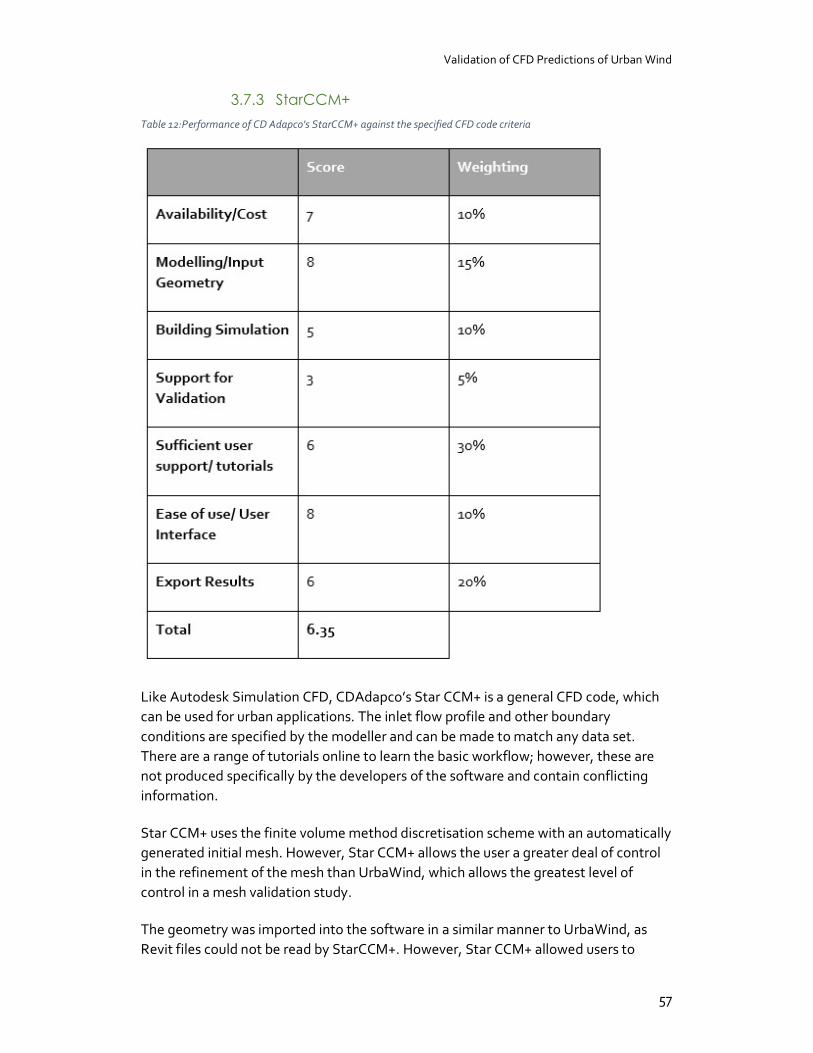
Validation of CFD Predictions of Urban Wind
57
3.7.3 StarCCM+
Table 12:Performance of CD Adapco's StarCCM+ against the specified CFD code criteria
Like Autodesk Simulation CFD, CDAdapco’s Star CCM+ is a general CFD code, which can be used for urban applications. The inlet flow profile and other boundary conditions are specified by the modeller and can be made to match any data set. There are a range of tutorials online to learn the basic workflow; however, these are not produced specifically by the developers of the software and contain conflicting information.
Star CCM+ uses the finite volume method discretisation scheme with an automatically generated initial mesh. However, Star CCM+ allows the user a greater deal of control in the refinement of the mesh than UrbaWind, which allows the greatest level of control in a mesh validation study.
The geometry was imported into the software in a similar manner to UrbaWind, as Revit files could not be read by StarCCM+. However, Star CCM+ allowed users to

Validation of CFD Predictions of Urban Wind
58
create geometry and move within the program. This gave a higher score in the import geometry category, as it allowed minor adjustments to be made without reverting to another piece of software.
Several validation studies have been carried out for Star CCM+, however none that involved validation of external aerodynamics in cities could be found.
3.7.4 Code selection
From the comparison tests above, Autodesk CFD was chosen as to run the validation studies. The deciding factors in this choice were the widely available user support and tutorials, and Simulation CFD having the simplest workflow.
Exporting the data was an issue which was identified as needing to be carefully controlled. This was to ensure that the measurement and CFD point comparisons were taken as close to the same points as possible.
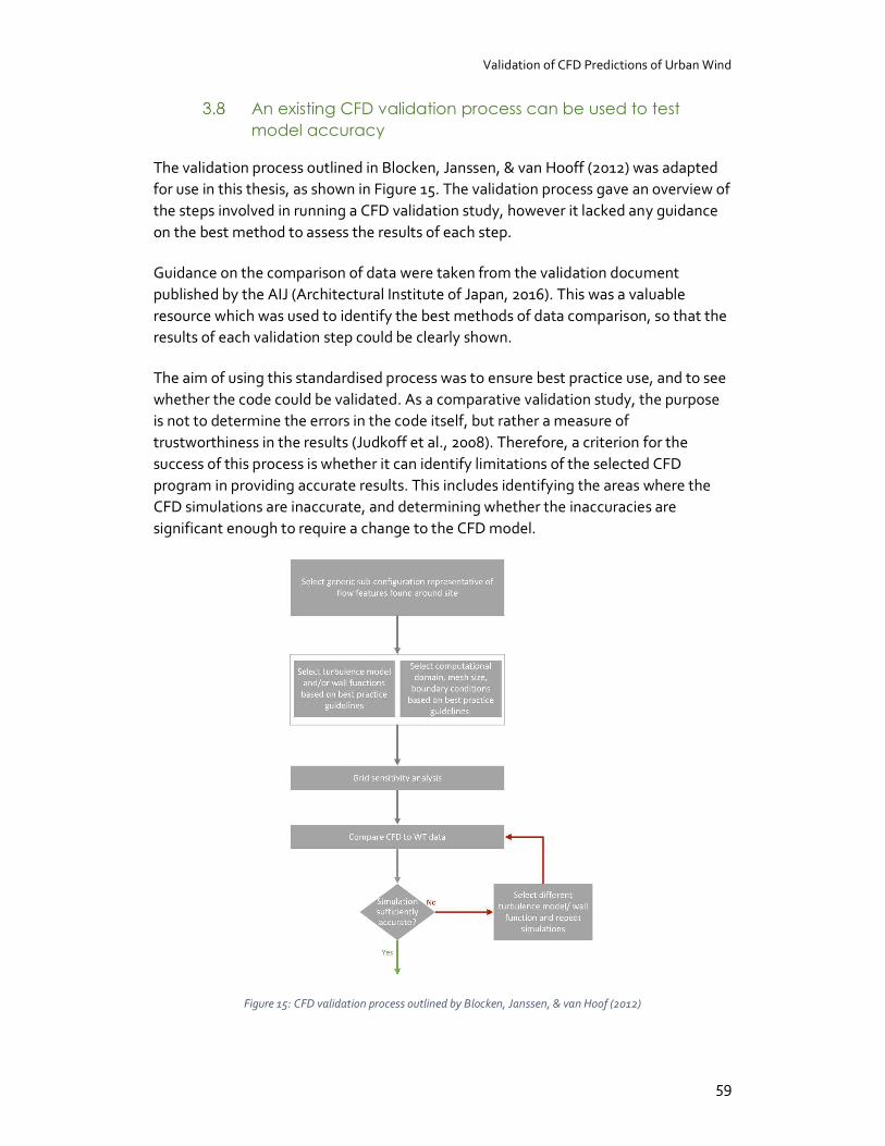
Validation of CFD Predictions of Urban Wind
59
An existing CFD validation process can be used to test model accuracy
The validation process outlined in Blocken, Janssen, & van Hooff (2012) was adapted for use in this thesis, as shown in Figure 15. The validation process gave an overview of the steps involved in running a CFD validation study, however it lacked any guidance on the best method to assess the results of each step.
Guidance on the comparison of data were taken from the validation document published by the AIJ (Architectural Institute of Japan, 2016). This was a valuable resource which was used to identify the best methods of data comparison, so that the results of each validation step could be clearly shown.
The aim of using this standardised process was to ensure best practice use, and to see whether the code could be validated. As a comparative validation study, the purpose is not to determine the errors in the code itself, but rather a measure of trustworthiness in the results (Judkoff et al., 2008). Therefore, a criterion for the success of this process is whether it can identify limitations of the selected CFD program in providing accurate results. This includes identifying the areas where the CFD simulations are inaccurate, and determining whether the inaccuracies are significant enough to require a change to the CFD model.
Figure 15: CFD validation process outlined by Blocken, Janssen, & van Hoof (2012)
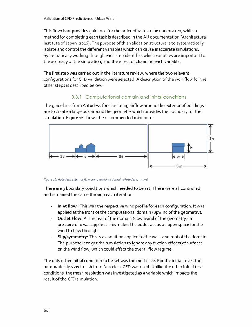
Validation of CFD Predictions of Urban Wind
60
This flowchart provides guidance for the order of tasks to be undertaken, while a method for completing each task is described in the AIJ documentation (Architectural Institute of Japan, 2016). The purpose of this validation structure is to systematically isolate and control the different variables which can cause inaccurate simulations. Systematically working through each step identifies which variables are important to the accuracy of the simulation, and the effect of changing each variable.
The first step was carried out in the literature review, where the two relevant configurations for CFD validation were selected. A description of the workflow for the other steps is described below:
3.8.1 Computational domain and initial conditions
The guidelines from Autodesk for simulating airflow around the exterior of buildings are to create a large box around the geometry which provides the boundary for the simulation. Figure 16 shows the recommended minimum
Figure 16: Autodesk external flow computational domain (Autodesk, n.d.-e)
There are 3 boundary conditions which needed to be set. These were all controlled and remained the same through each iteration:
- Inlet flow: This was the respective wind profile for each configuration. It was applied at the front of the computational domain (upwind of the geometry).
- Outlet Flow: At the rear of the domain (downwind of the geometry), a pressure of 0 was applied. This makes the outlet act as an open space for the wind to flow through.
- Slip/symmetry: This is a condition applied to the walls and roof of the domain. The purpose is to get the simulation to ignore any friction effects of surfaces on the wind flow, which could affect the overall flow regime.
The only other initial condition to be set was the mesh size. For the initial tests, the automatically sized mesh from Autodesk CFD was used. Unlike the other initial test conditions, the mesh resolution was investigated as a variable which impacts the result of the CFD simulation.

Validation of CFD Predictions of Urban Wind
61
3.8.2 Mesh sensitivity analysis
The documentation for Simulation CFD describes the automatic meshing process: “Autodesk® CFD performs a comprehensive topological interrogation of the analysis geometry and determines the mesh size and distribution on every edge, surface, and volume in the model” (Autodesk, n.d.-a).
As well as automatically generating the mesh, Simulation CFD allows users to refine the mesh using a slider, or by entering a factor by which to multiply the mesh. A factor of less than 1 increases the mesh resolution, while factors of greater than 1 cause the mesh to be coarser.
The mesh validation process was identical for each simulation. Taking the automatic resolution as the coarsest mesh, further iterations at a factor of 0.5, 0.25, 0.2 and 0.15 were carried out. The results were graphed and compared to find the point where the simulation reached mesh independence, and further increases to the mesh resolution did not significantly alter the simulation results.
As well as comparing each CFD iteration, the results were graphed against the truth model from the wind tunnel. This showed whether the mesh resolution was a variable which brought the result significantly closer to the wind tunnel results.
3.8.3 A description of the various turbulence models
The final variable in the validation process was the selection of an appropriate turbulence model. As described in Section 2.7.1, there are a range of turbulence models that have been developed to calculate air flows in different applications.
The purpose of time-averaging the flow calculation in the RANS simulation method is to remove the need to explicitly calculate turbulent air behaviour. However, to account for the effect that turbulence has on the overall flow features, turbulence models are used. In terms of the calculations involved in solving a CFD simulation, turbulence models can be thought of as “modelling assumptions” (Blocken et al., 2016).
From the range provided using Autodesk Simulation CFD, the models in Table 13 were selected for further investigation.
Validation of CFD Predictions of Urban Wind
62
Table 13: Turbulence model comparison
Each of these turbulence models were simulated at the optimal mesh resolution as determined by the mesh sensitivity analysis, and the results were compared to the wind tunnel tests. The turbulence model is the last variable to be compared using the validation process, so any other changes are outside of the recommended process.
3.8.4 Data Analysis
Two types of graphs were used in the analysis: line graphs and scatter plots. Examples of each graph type and why they are important to the analysis are given below:
Line Graphs
Figure 17 shows the how the line graphs compare the wind tunnel and CFD results. The dashed green line represents the truth model, while the blue line shows the CFD analysis. Each number along the x-axis corresponds to a measurement point taken in the wind tunnel. These numbers are largely irrelevant, as the focus of the validation process is how well the CFD graphs fit the dashed wind tunnel graph. However, they provide a useful reference point back to the measurement points.
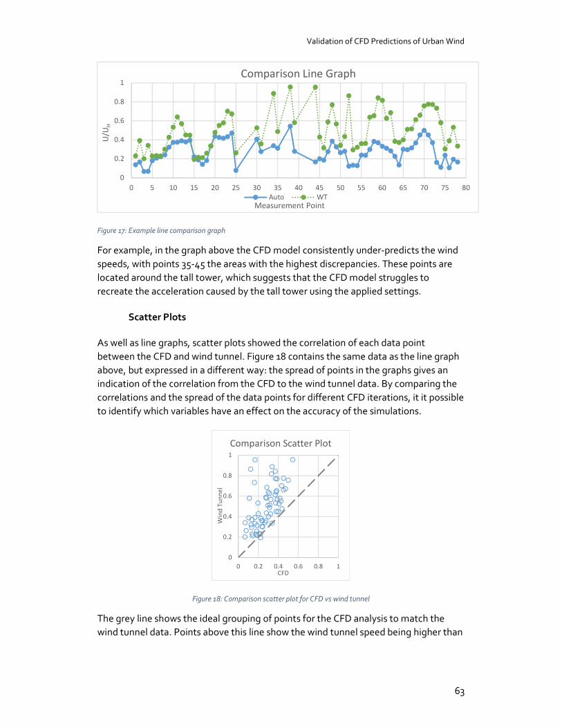
Validation of CFD Predictions of Urban Wind
63
Figure 17: Example line comparison graph
For example, in the graph above the CFD model consistently under-predicts the wind speeds, with points 35-45 the areas with the highest discrepancies. These points are located around the tall tower, which suggests that the CFD model struggles to recreate the acceleration caused by the tall tower using the applied settings.
Scatter Plots
As well as line graphs, scatter plots showed the correlation of each data point between the CFD and wind tunnel. Figure 18 contains the same data as the line graph above, but expressed in a different way: the spread of points in the graphs gives an indication of the correlation from the CFD to the wind tunnel data. By comparing the correlations and the spread of the data points for different CFD iterations, it it possible to identify which variables have an effect on the accuracy of the simulations.
Figure 18: Comparison scatter plot for CFD vs wind tunnel
The grey line shows the ideal grouping of points for the CFD analysis to match the wind tunnel data. Points above this line show the wind tunnel speed being higher than
0
0.2
0.4
0.6
0.8
1
0 5 10 15 20 25 30 35 40 45 50 55 60 65 70 75 80
U/U
H
Measurement Point
Comparison Line Graph
Auto WT
0
0.2
0.4
0.6
0.8
1
0 0.2 0.4 0.6 0.8 1
Win
d Tu
nnel
CFD
Comparison Scatter Plot
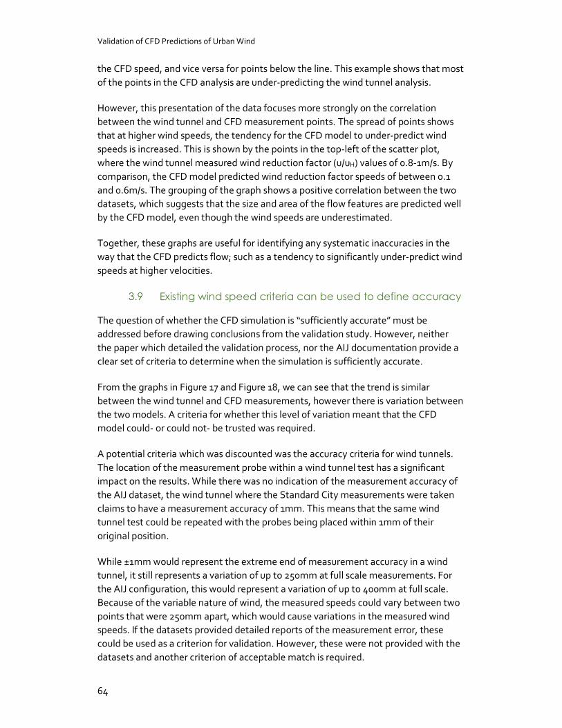
Validation of CFD Predictions of Urban Wind
64
the CFD speed, and vice versa for points below the line. This example shows that most of the points in the CFD analysis are under-predicting the wind tunnel analysis.
However, this presentation of the data focuses more strongly on the correlation between the wind tunnel and CFD measurement points. The spread of points shows that at higher wind speeds, the tendency for the CFD model to under-predict wind speeds is increased. This is shown by the points in the top-left of the scatter plot, where the wind tunnel measured wind reduction factor (u/uH) values of 0.8-1m/s. By comparison, the CFD model predicted wind reduction factor speeds of between 0.1 and 0.6m/s. The grouping of the graph shows a positive correlation between the two datasets, which suggests that the size and area of the flow features are predicted well by the CFD model, even though the wind speeds are underestimated.
Together, these graphs are useful for identifying any systematic inaccuracies in the way that the CFD predicts flow; such as a tendency to significantly under-predict wind speeds at higher velocities.
Existing wind speed criteria can be used to define accuracy
The question of whether the CFD simulation is “sufficiently accurate” must be addressed before drawing conclusions from the validation study. However, neither the paper which detailed the validation process, nor the AIJ documentation provide a clear set of criteria to determine when the simulation is sufficiently accurate.
From the graphs in Figure 17 and Figure 18, we can see that the trend is similar between the wind tunnel and CFD measurements, however there is variation between the two models. A criteria for whether this level of variation meant that the CFD model could- or could not- be trusted was required.
A potential criteria which was discounted was the accuracy criteria for wind tunnels. The location of the measurement probe within a wind tunnel test has a significant impact on the results. While there was no indication of the measurement accuracy of the AIJ dataset, the wind tunnel where the Standard City measurements were taken claims to have a measurement accuracy of 1mm. This means that the same wind tunnel test could be repeated with the probes being placed within 1mm of their original position.
While ±1mm would represent the extreme end of measurement accuracy in a wind tunnel, it still represents a variation of up to 250mm at full scale measurements. For the AIJ configuration, this would represent a variation of up to 400mm at full scale. Because of the variable nature of wind, the measured speeds could vary between two points that were 250mm apart, which would cause variations in the measured wind speeds. If the datasets provided detailed reports of the measurement error, these could be used as a criterion for validation. However, these were not provided with the datasets and another criterion of acceptable match is required.

Validation of CFD Predictions of Urban Wind
65
One such criterion is whether the design recommendations would be changed if the CFD simulation was used instead of the wind tunnel data. To test this, a wind criteria was selected which could identify when the variation between the CFD and wind tunnel data would require a change in design. The acceptability criteria used by Wellington City Council is an internationally recognised standard which uses a measure known as the effective gust speeds to determine wind acceptability (Carpenter, 2002). An alternative option was the Lawson criteria- which are used widely in the UK- and are based on mean speeds, gust speeds and hours of exceedance (Shilston, 2015).
The WCC criteria were selected for use in this thesis, as they were directly relevant to Wellington city. However, for the applicability of the validation process to international cities, a description and assessment using the Lawson criteria is included in Appendix I: Results of CFD simulations
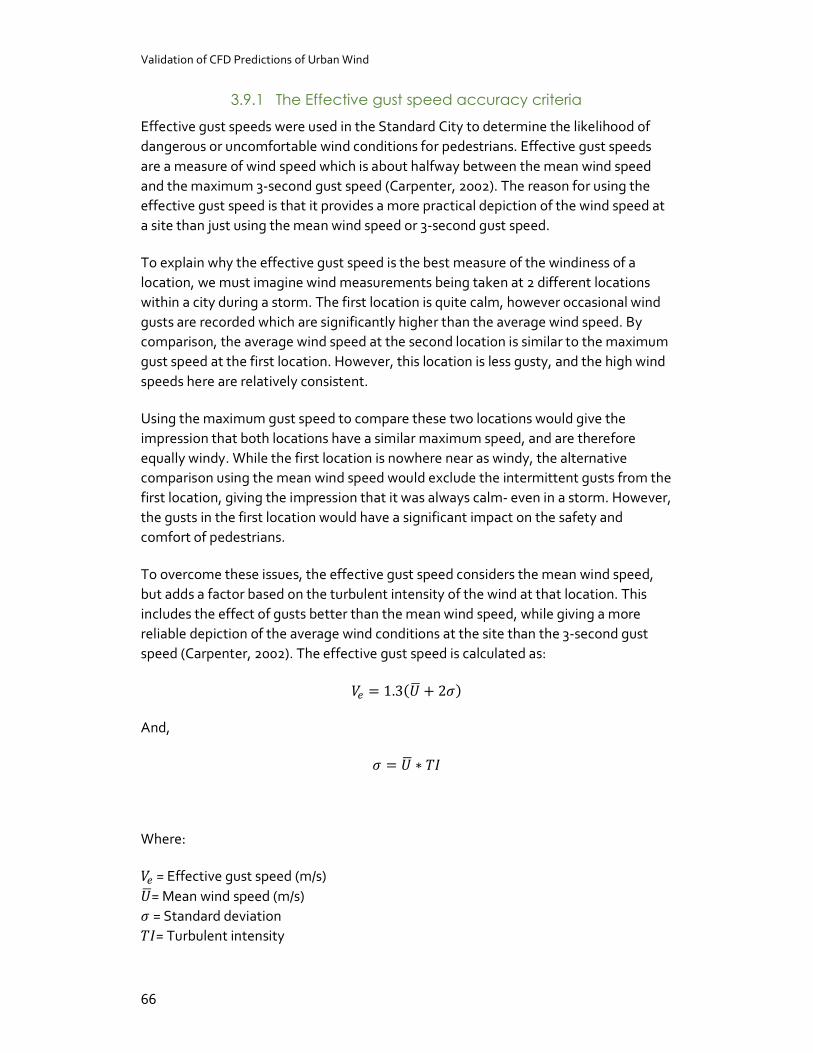
Validation of CFD Predictions of Urban Wind
66
3.9.1 The Effective gust speed accuracy criteria
Effective gust speeds were used in the Standard City to determine the likelihood of dangerous or uncomfortable wind conditions for pedestrians. Effective gust speeds are a measure of wind speed which is about halfway between the mean wind speed and the maximum 3-second gust speed (Carpenter, 2002). The reason for using the effective gust speed is that it provides a more practical depiction of the wind speed at a site than just using the mean wind speed or 3-second gust speed.
To explain why the effective gust speed is the best measure of the windiness of a location, we must imagine wind measurements being taken at 2 different locations within a city during a storm. The first location is quite calm, however occasional wind gusts are recorded which are significantly higher than the average wind speed. By comparison, the average wind speed at the second location is similar to the maximum gust speed at the first location. However, this location is less gusty, and the high wind speeds here are relatively consistent.
Using the maximum gust speed to compare these two locations would give the impression that both locations have a similar maximum speed, and are therefore equally windy. While the first location is nowhere near as windy, the alternative comparison using the mean wind speed would exclude the intermittent gusts from the first location, giving the impression that it was always calm- even in a storm. However, the gusts in the first location would have a significant impact on the safety and comfort of pedestrians.
To overcome these issues, the effective gust speed considers the mean wind speed, but adds a factor based on the turbulent intensity of the wind at that location. This includes the effect of gusts better than the mean wind speed, while giving a more reliable depiction of the average wind conditions at the site than the 3-second gust speed (Carpenter, 2002). The effective gust speed is calculated as:
= 1.3 + 2
And,
= ∗
Where:
= Effective gust speed (m/s) = Mean wind speed (m/s) = Standard deviation = Turbulent intensity
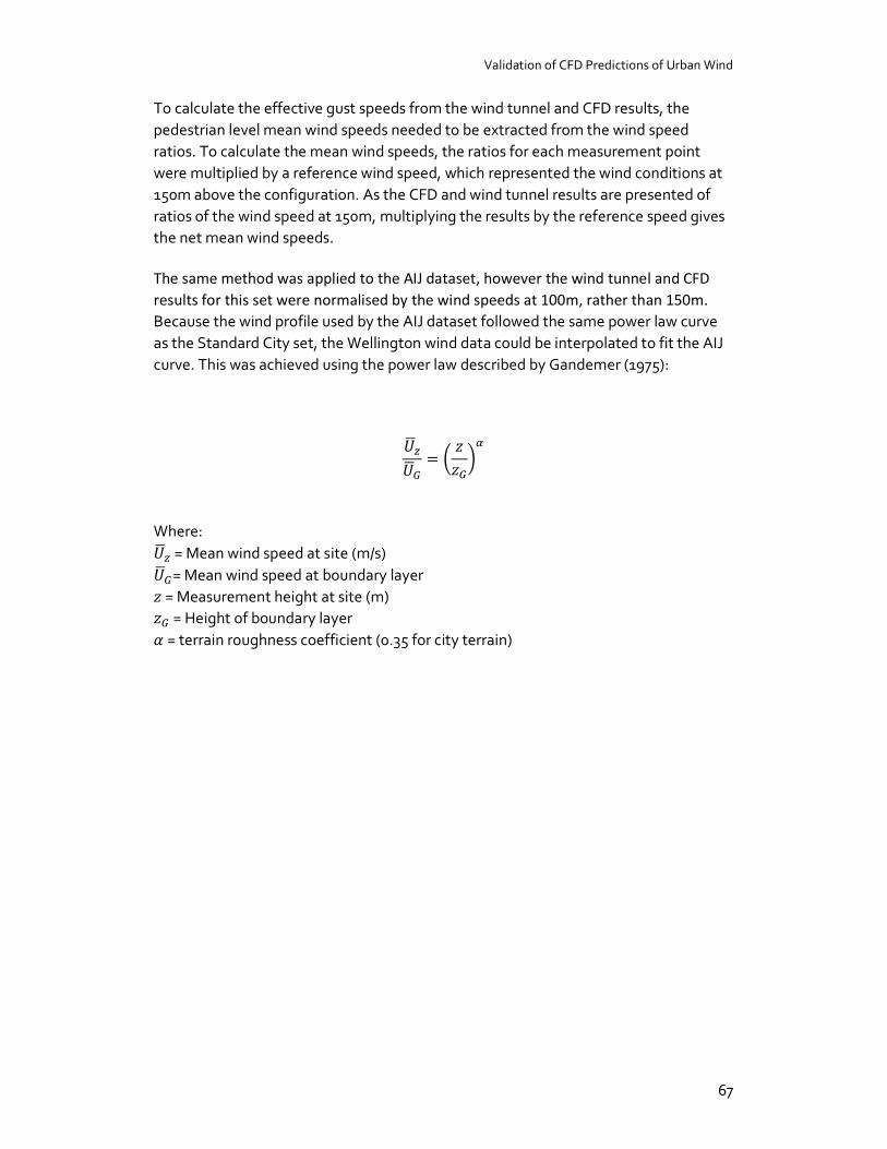
Validation of CFD Predictions of Urban Wind
67
To calculate the effective gust speeds from the wind tunnel and CFD results, the pedestrian level mean wind speeds needed to be extracted from the wind speed ratios. To calculate the mean wind speeds, the ratios for each measurement point were multiplied by a reference wind speed, which represented the wind conditions at 150m above the configuration. As the CFD and wind tunnel results are presented of ratios of the wind speed at 150m, multiplying the results by the reference speed gives the net mean wind speeds.
The same method was applied to the AIJ dataset, however the wind tunnel and CFD results for this set were normalised by the wind speeds at 100m, rather than 150m. Because the wind profile used by the AIJ dataset followed the same power law curve as the Standard City set, the Wellington wind data could be interpolated to fit the AIJ curve. This was achieved using the power law described by Gandemer (1975):
=
Where:
= Mean wind speed at site (m/s) = Mean wind speed at boundary layer
= Measurement height at site (m) = Height of boundary layer
= terrain roughness coefficient (0.35 for city terrain)
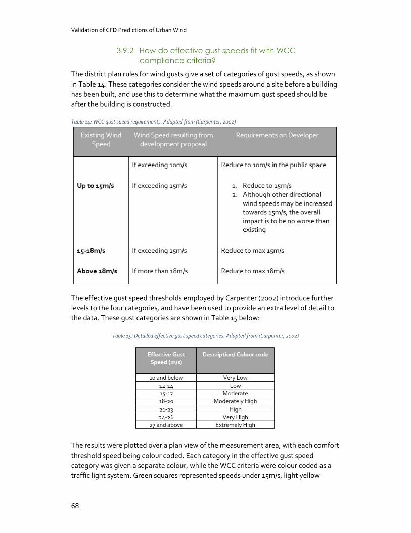
Validation of CFD Predictions of Urban Wind
68
3.9.2 How do effective gust speeds fit with WCC compliance criteria?
The district plan rules for wind gusts give a set of categories of gust speeds, as shown in Table 14. These categories consider the wind speeds around a site before a building has been built, and use this to determine what the maximum gust speed should be after the building is constructed.
Table 14: WCC gust speed requirements. Adapted from (Carpenter, 2002)
The effective gust speed thresholds employed by Carpenter (2002) introduce further levels to the four categories, and have been used to provide an extra level of detail to the data. These gust categories are shown in Table 15 below:
Table 15: Detailed effective gust speed categories. Adapted from (Carpenter, 2002)
The results were plotted over a plan view of the measurement area, with each comfort threshold speed being colour coded. Each category in the effective gust speed category was given a separate colour, while the WCC criteria were colour coded as a traffic light system. Green squares represented speeds under 15m/s, light yellow
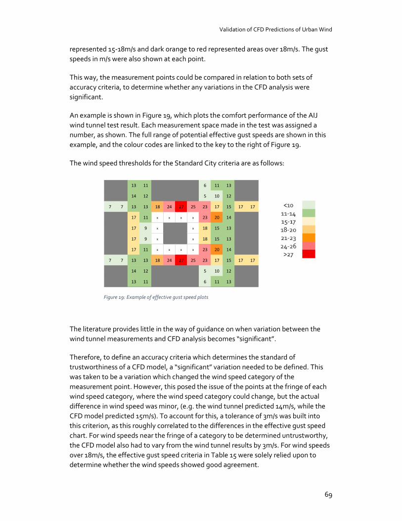
Validation of CFD Predictions of Urban Wind
69
represented 15-18m/s and dark orange to red represented areas over 18m/s. The gust speeds in m/s were also shown at each point.
This way, the measurement points could be compared in relation to both sets of accuracy criteria, to determine whether any variations in the CFD analysis were significant.
An example is shown in Figure 19, which plots the comfort performance of the AIJ wind tunnel test result. Each measurement space made in the test was assigned a number, as shown. The full range of potential effective gust speeds are shown in this example, and the colour codes are linked to the key to the right of Figure 19.
The wind speed thresholds for the Standard City criteria are as follows:
The literature provides little in the way of guidance on when variation between the wind tunnel measurements and CFD analysis becomes “significant”.
Therefore, to define an accuracy criteria which determines the standard of trustworthiness of a CFD model, a “significant” variation needed to be defined. This was taken to be a variation which changed the wind speed category of the measurement point. However, this posed the issue of the points at the fringe of each wind speed category, where the wind speed category could change, but the actual difference in wind speed was minor, (e.g. the wind tunnel predicted 14m/s, while the CFD model predicted 15m/s). To account for this, a tolerance of 3m/s was built into this criterion, as this roughly correlated to the differences in the effective gust speed chart. For wind speeds near the fringe of a category to be determined untrustworthy, the CFD model also had to vary from the wind tunnel results by 3m/s. For wind speeds over 18m/s, the effective gust speed criteria in Table 15 were solely relied upon to determine whether the wind speeds showed good agreement.
13 11 6 11 13
14 12 5 10 12
7 7 13 13 18 24 27 25 23 17 15 17 17
17 11 x x x x 23 20 14
17 9 x x 18 15 13
17 9 x x 18 15 13
17 11 x x x x 23 20 14
7 7 13 13 18 24 27 25 23 17 15 17 17
14 12 5 10 12
13 11 6 11 13
Figure 19: Example of effective gust speed plots

Validation of CFD Predictions of Urban Wind
70
Finally, in terms of validation, a small number of inaccurate points scattered around the configuration do not necessarily reflect a systematic inaccuracy of the CFD simulation. However, if there were groupings of points where the CFD results are inaccurate, this suggests a problem with the CFD solution. Similarly, where points in similar areas (e.g. immediately behind the buildings) are repeatedly inaccurately modelling the wind, this suggests that there is a systematic inaccuracy with the CFD code.
The measurement points in each configuration were broken up into clusters to better describe the flow features. To validate the flows, at least half of the points in each cluster needed to meet the accuracy criteria. If any cluster in the configuration did not meet the accuracy criteria, this meant that the CFD model was not properly recreating the flows.
71
4. Determining Appropriate Parameters for the CFD Validation Study
As described in Chapter 3, the validation methodology is essentially a set of CFD iterative studies. A series of analyses was conducted comparing the wind tunnel results of the AIJ and Standard City urban configurations against CFD analyses with different mesh size, turbulence and boundary conditions. The goal was to establish whether this process could determine an acceptable match between CFD and wind tunnel data. This chapter details the execution of the process, and the changes that were required as the case study was carried out.
To compare the simulation results as shown in the CFD software, images from the CFD simulations were included in Appendix I.
A test using the AIJ simple block
The initial test using the 2:1:1 AIJ block configuration was used to test whether Autodesk CFD could recreate the flow features around a simple geometric shape. The data for the single block was provided as vector measurements pf the flow in the x, y and z directions. This allowed an assessment to be made of the CFD model’s accuracy for both the magnitude of the wind speed, and direction of the flow.
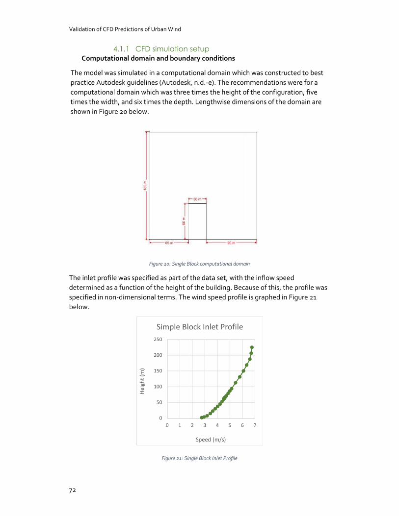
Validation of CFD Predictions of Urban Wind
72
4.1.1 CFD simulation setup Computational domain and boundary conditions
The model was simulated in a computational domain which was constructed to best practice Autodesk guidelines (Autodesk, n.d.-e). The recommendations were for a computational domain which was three times the height of the configuration, five times the width, and six times the depth. Lengthwise dimensions of the domain are shown in Figure 20 below.
Figure 20: Single Block computational domain
The inlet profile was specified as part of the data set, with the inflow speed determined as a function of the height of the building. Because of this, the profile was specified in non-dimensional terms. The wind speed profile is graphed in Figure 21 below.
Figure 21: Single Block Inlet Profile
0
50
100
150
200
250
0 1 2 3 4 5 6 7
Hei
ght (
m)
Speed (m/s)
Simple Block Inlet Profile
Validation of CFD Predictions of Urban Wind
73
As well as the inlet wind speed profile, a pressure condition of zero was specified at the outlet, to make the fluid flow through the space as it would in an open area.
In both the CFD and wind tunnel tests, the wind being simulated around the building model is effectively flowing through a large duct. Bounding the wind flow in with walls and a ceiling causes a build-up of pressure and frictional drag around the edges of the wind tunnel or CFD domain. This can cause differences between the modelled flow and real-world flows, as real-world flows are not bounded by walls. In the wind tunnel, the effects of the walls on the flow are mitigated by placing the model in the centre of the wind tunnel, and ensuring that the model does not take up more than 10% of the cross-sectional area (Irwin, Denoon, & Scott, 2013). This means that the flow passing over the model will be an accurate representation of free-field flow.
In CFD modelling, there are 3 methods used which reduce the effect of the boundary area on the simulation results. The first is appropriately sizing the computational domain, as illustrated previously in Figure 20. The second method is to apply slip/symmetry conditions to the inside walls and ceiling of the computational domain. The purpose of these conditions is to negate the frictional effects, and reduce the impact of the boundary walls on the CFD simulation (Autodesk, n.d.-d). The final method is to remove the mesh from the walls, which omits them from the calculation (Autodesk, n.d.-f). This effectively negates the effect of the boundary walls. Autodesk best practice guidance recommends all 3 steps be taken (Autodesk, n.d.-e; Wilde, 2015).
Mesh sizes
Table 16 shows the range of mesh sizes which were used to run the mesh sensitivity analysis for the 2:1:1 block analysis. The left-hand column shows the mesh resolutions which were used. Autodesk CFD automatically generates an unstructured tetrahedral mesh1. The automatically sized mesh was used as the first iteration. Further iterations of mesh resolution could be selected using a slider. Values of less than 1 indicate a finer mesh resolution, whole values of more than 1 indicate a coarser mesh resolution. Mesh resolutions of 0.5 and 0.2 were selected to compare to the automatically sized mesh.
Along with the images of each mesh in the centre column, the number of calculation points was shown in in the right-hand column. The table shows that increasing the mesh resolution significantly increases the number of calculation points. Where one would expect that the 0.5 mesh would give a mesh resolution that was twice as fine as the automatically sized mesh, the calculation point count is different by a factor of around 5. As discussed in Section 2.7.2, an increase in mesh size requires more
1 An unstructured tetrahedral mesh is made up of irregular triangular elements. This is unlike a regular grid, which is made up of uniform rectangular elements that vary evenly in size.
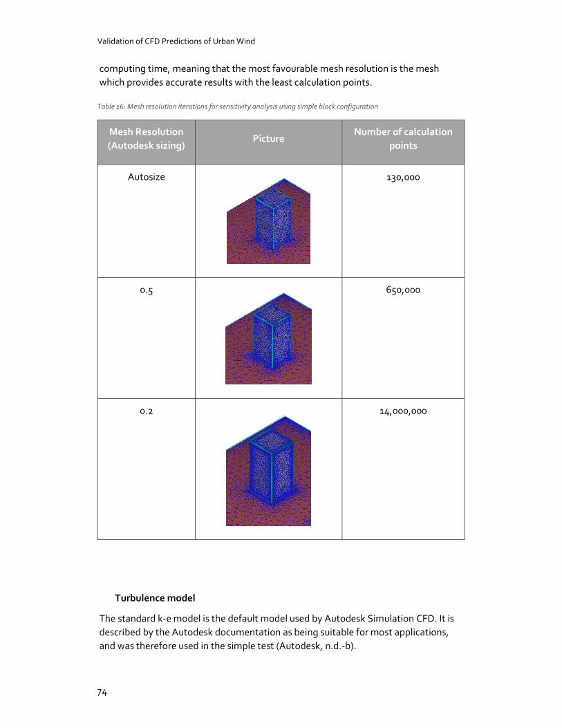
Validation of CFD Predictions of Urban Wind
74
computing time, meaning that the most favourable mesh resolution is the mesh which provides accurate results with the least calculation points.
Table 16: Mesh resolution iterations for sensitivity analysis using simple block configuration
Mesh Resolution (Autodesk sizing)
Picture Number of calculation
points
Autosize
130,000
0.5
650,000
0.2
14,000,000
Turbulence model
The standard k-e model is the default model used by Autodesk Simulation CFD. It is described by the Autodesk documentation as being suitable for most applications, and was therefore used in the simple test (Autodesk, n.d.-b).
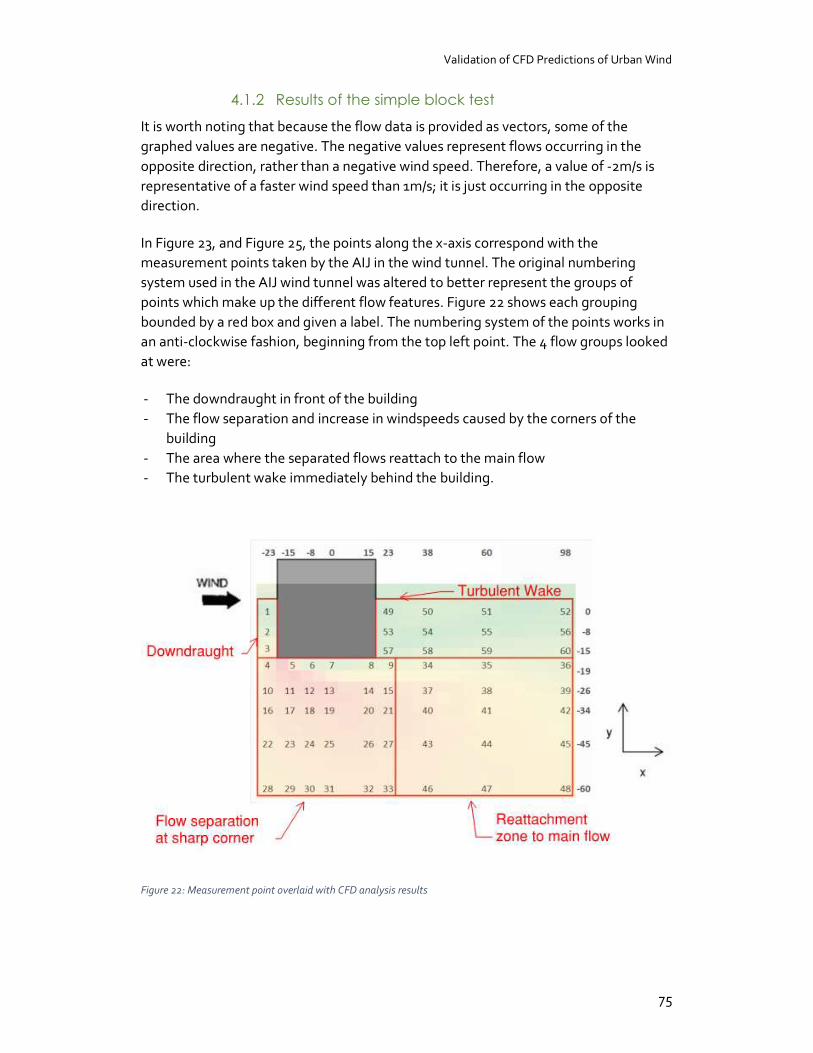
Validation of CFD Predictions of Urban Wind
75
4.1.2 Results of the simple block test
It is worth noting that because the flow data is provided as vectors, some of the graphed values are negative. The negative values represent flows occurring in the opposite direction, rather than a negative wind speed. Therefore, a value of -2m/s is representative of a faster wind speed than 1m/s; it is just occurring in the opposite direction.
In Figure 23, and Figure 25, the points along the x-axis correspond with the measurement points taken by the AIJ in the wind tunnel. The original numbering system used in the AIJ wind tunnel was altered to better represent the groups of points which make up the different flow features. Figure 22 shows each grouping bounded by a red box and given a label. The numbering system of the points works in an anti-clockwise fashion, beginning from the top left point. The 4 flow groups looked at were:
- The downdraught in front of the building - The flow separation and increase in windspeeds caused by the corners of the
building - The area where the separated flows reattach to the main flow - The turbulent wake immediately behind the building.
Figure 22: Measurement point overlaid with CFD analysis results
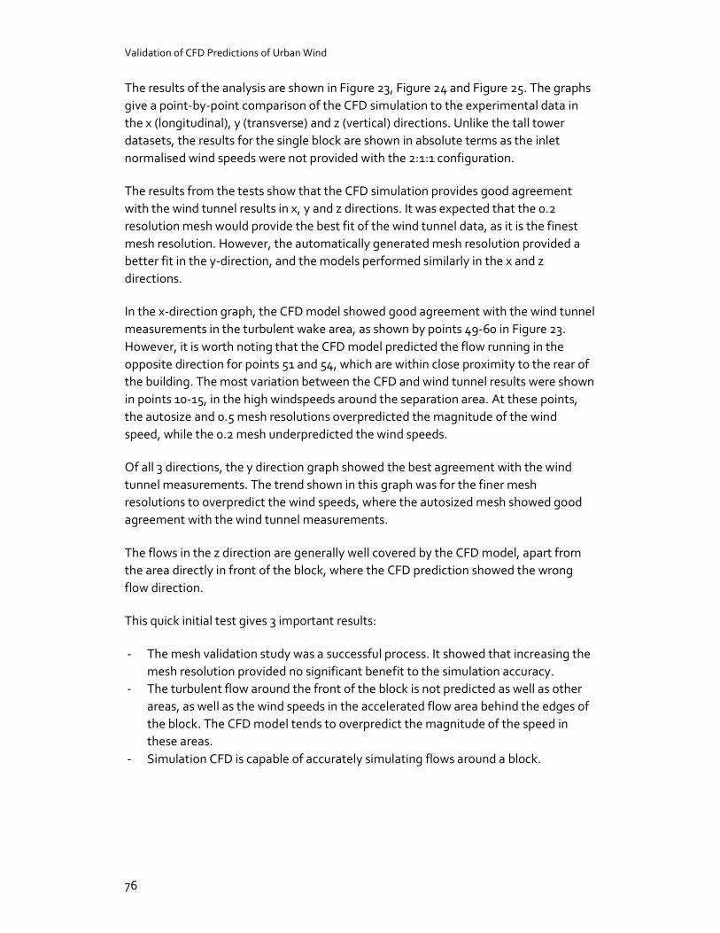
Validation of CFD Predictions of Urban Wind
76
The results of the analysis are shown in Figure 23, Figure 24 and Figure 25. The graphs give a point-by-point comparison of the CFD simulation to the experimental data in the x (longitudinal), y (transverse) and z (vertical) directions. Unlike the tall tower datasets, the results for the single block are shown in absolute terms as the inlet normalised wind speeds were not provided with the 2:1:1 configuration.
The results from the tests show that the CFD simulation provides good agreement with the wind tunnel results in x, y and z directions. It was expected that the 0.2 resolution mesh would provide the best fit of the wind tunnel data, as it is the finest mesh resolution. However, the automatically generated mesh resolution provided a better fit in the y-direction, and the models performed similarly in the x and z directions.
In the x-direction graph, the CFD model showed good agreement with the wind tunnel measurements in the turbulent wake area, as shown by points 49-60 in Figure 23. However, it is worth noting that the CFD model predicted the flow running in the opposite direction for points 51 and 54, which are within close proximity to the rear of the building. The most variation between the CFD and wind tunnel results were shown in points 10-15, in the high windspeeds around the separation area. At these points, the autosize and 0.5 mesh resolutions overpredicted the magnitude of the wind speed, while the 0.2 mesh underpredicted the wind speeds.
Of all 3 directions, the y direction graph showed the best agreement with the wind tunnel measurements. The trend shown in this graph was for the finer mesh resolutions to overpredict the wind speeds, where the autosized mesh showed good agreement with the wind tunnel measurements.
The flows in the z direction are generally well covered by the CFD model, apart from the area directly in front of the block, where the CFD prediction showed the wrong flow direction.
This quick initial test gives 3 important results:
- The mesh validation study was a successful process. It showed that increasing the mesh resolution provided no significant benefit to the simulation accuracy.
- The turbulent flow around the front of the block is not predicted as well as other areas, as well as the wind speeds in the accelerated flow area behind the edges of the block. The CFD model tends to overpredict the magnitude of the speed in these areas.
- Simulation CFD is capable of accurately simulating flows around a block.
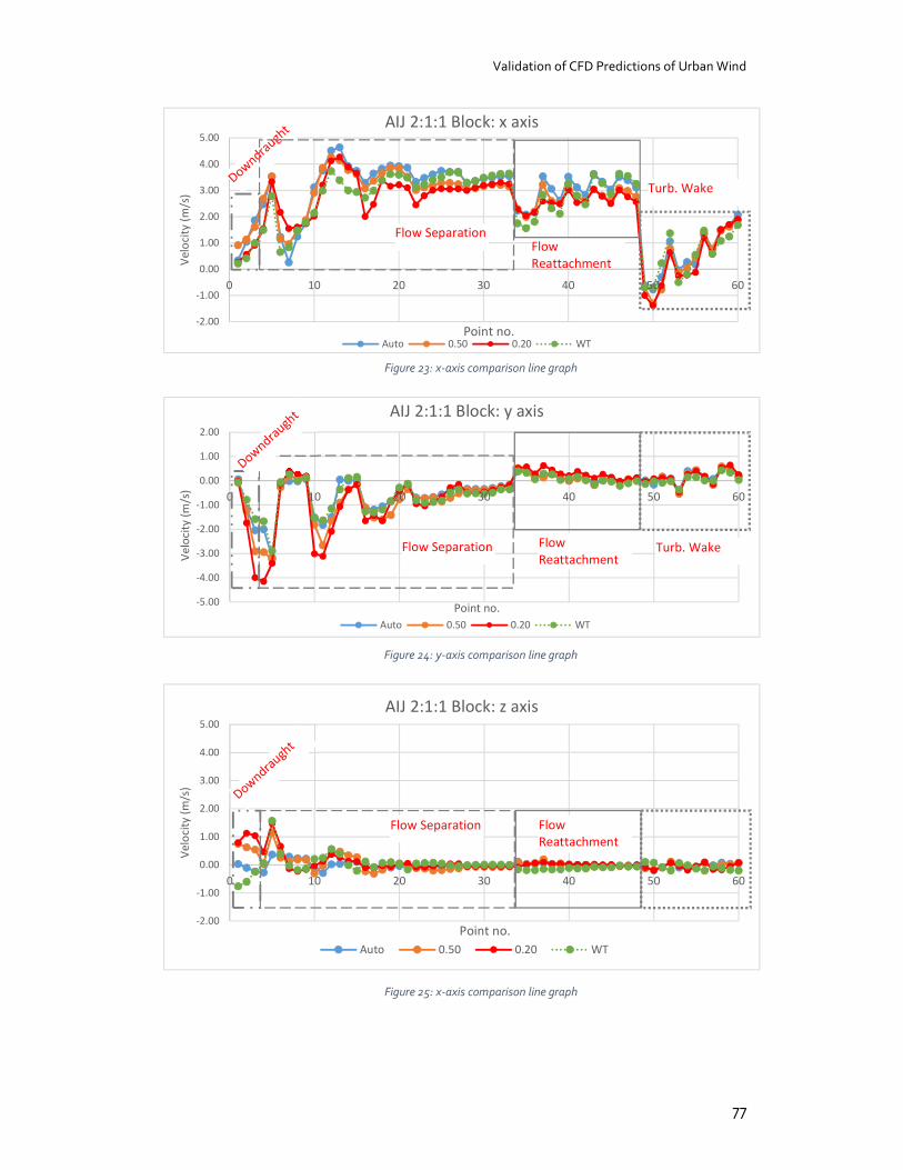
Validation of CFD Predictions of Urban Wind
77
Figure 23: x-axis comparison line graph
Figure 24: y-axis comparison line graph
Figure 25: x-axis comparison line graph
-2.00
-1.00
0.00
1.00
2.00
3.00
4.00
5.00
0 10 20 30 40 50 60
Velo
city
(m/s
)
Point no.
AIJ 2:1:1 Block: x axis
Auto 0.50 0.20 WT
Flow SeparationFlow Reattachment
Turb. Wake
-5.00
-4.00
-3.00
-2.00
-1.00
0.00
1.00
2.00
0 10 20 30 40 50 60
Velo
city
(m/s
)
Point no.
AIJ 2:1:1 Block: y axis
Auto 0.50 0.20 WT
-2.00
-1.00
0.00
1.00
2.00
3.00
4.00
5.00
0 10 20 30 40 50 60
Velo
city
(m/s
)
Point no.
AIJ 2:1:1 Block: z axis
Auto 0.50 0.20 WT
Turb. Wake Flow Reattachment
Flow Reattachment
Flow Separation
Flow Separation
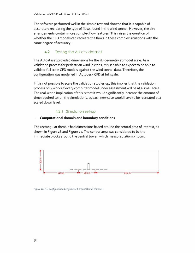
Validation of CFD Predictions of Urban Wind
78
The software performed well in the simple test and showed that it is capable of accurately recreating the type of flows found in the wind tunnel. However, the city arrangements contain more complex flow features. This raises the question of whether the CFD models can recreate the flows in these complex situations with the same degree of accuracy.
Testing the AIJ city dataset
The AIJ dataset provided dimensions for the 3D geometry at model scale. As a validation process for pedestrian wind in cities, it is sensible to expect to be able to validate full scale CFD models against the wind tunnel data. Therefore, the configuration was modelled in Autodesk CFD at full scale.
If it is not possible to scale the validation studies up, this implies that the validation process only works if every computer model under assessment will be at a small scale. The real-world implication of this is that it would significantly increase the amount of time required to run the simulations, as each new case would have to be recreated at a scaled down level.
4.2.1 Simulation set-up
- Computational domain and boundary conditions
The rectangular domain had dimensions based around the central area of interest, as shown in Figure 26 and Figure 27. The central area was considered to be the immediate blocks around the central tower, which measured 260m x 300m.
Figure 26: AIJ Configuration Lengthwise Computational Domain
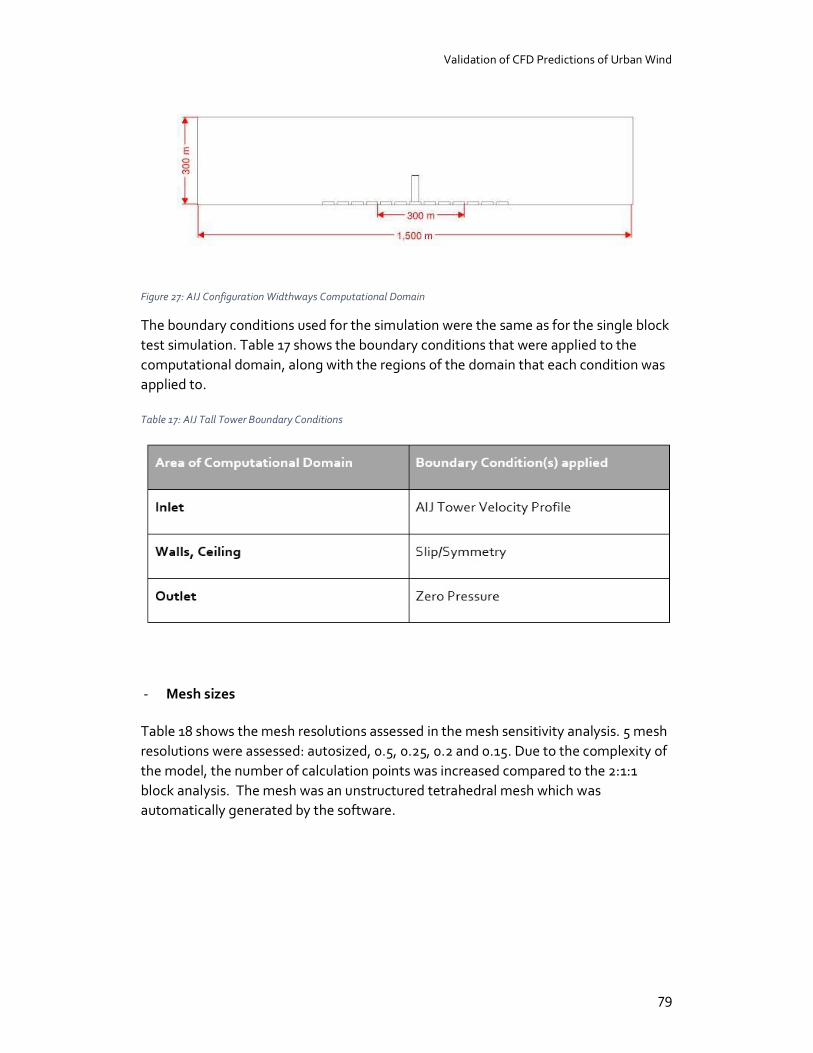
Validation of CFD Predictions of Urban Wind
79
Figure 27: AIJ Configuration Widthways Computational Domain
The boundary conditions used for the simulation were the same as for the single block test simulation. Table 17 shows the boundary conditions that were applied to the computational domain, along with the regions of the domain that each condition was applied to.
Table 17: AIJ Tall Tower Boundary Conditions
- Mesh sizes
Table 18 shows the mesh resolutions assessed in the mesh sensitivity analysis. 5 mesh resolutions were assessed: autosized, 0.5, 0.25, 0.2 and 0.15. Due to the complexity of the model, the number of calculation points was increased compared to the 2:1:1 block analysis. The mesh was an unstructured tetrahedral mesh which was automatically generated by the software.
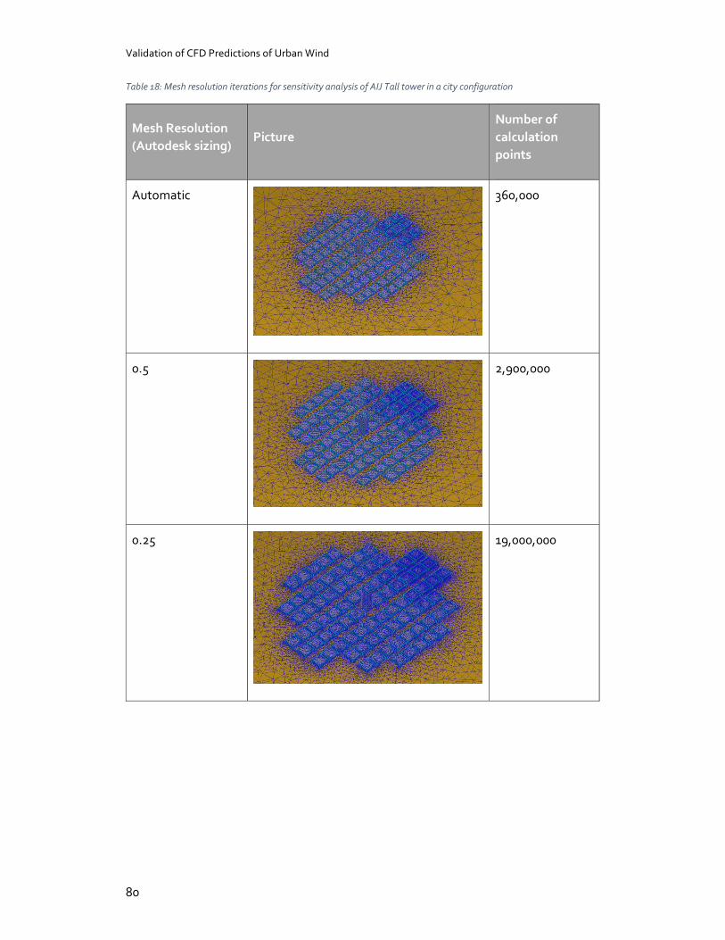
Validation of CFD Predictions of Urban Wind
80
Table 18: Mesh resolution iterations for sensitivity analysis of AIJ Tall tower in a city configuration
Mesh Resolution (Autodesk sizing)
Picture Number of calculation points
Automatic
360,000
0.5
2,900,000
0.25
19,000,000
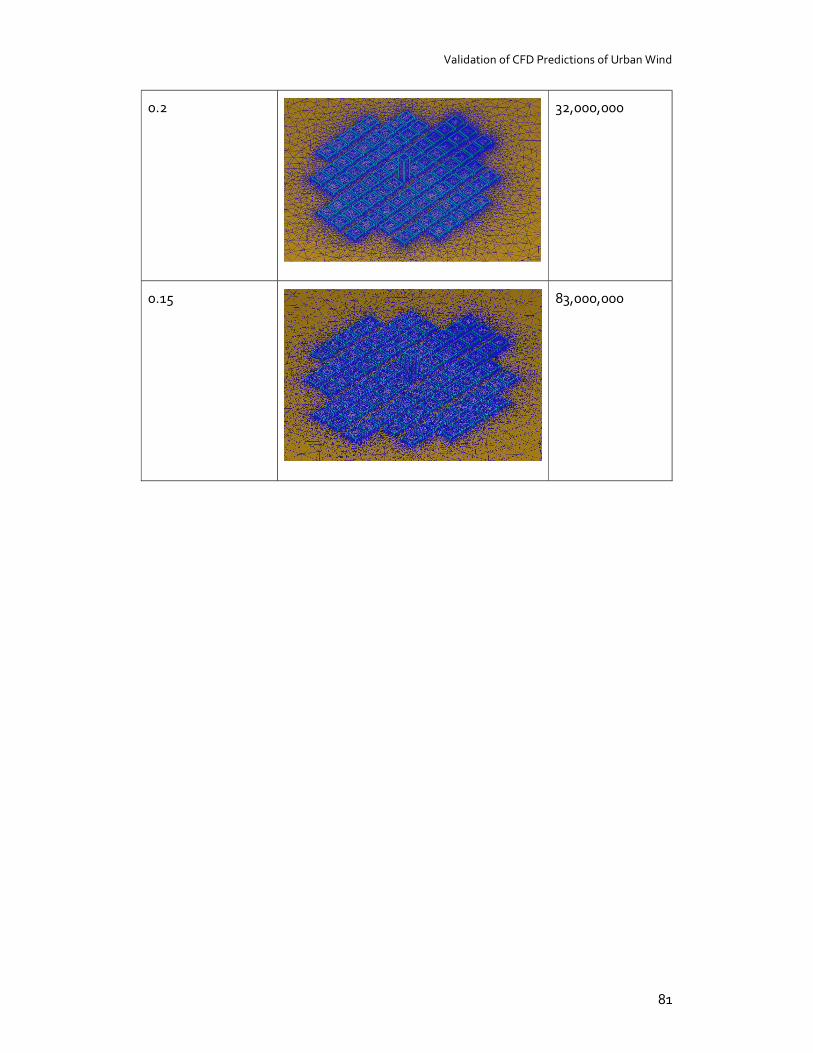
Validation of CFD Predictions of Urban Wind
81
0.2
32,000,000
0.15
83,000,000

Validation of CFD Predictions of Urban Wind
82
4.2.2 Grouping the measurement points helps to identify and compare the flow features
The validation process systematically assessed four variables to determine which had the largest impact on the accuracy of the CFD solution, and which settings should be used to model the urban flow in a city. The four variables which were assessed were: - Mesh Resolution - Turbulence model - Turbulent intensity factor, k - Whether the model was simulated at model scale or full scale
The AIJ tall tower configuration provided overall velocity as well as the x, y and z vectors. The overall wind speed is made up of the sum of the vectors, and provides a measure of how well the CFD fits the wind tunnel speed. However, it does not show whether CFD matches the wind direction. The comparison process consisted used the overall wind speed, as it removed the need to analyse the same points 3 times. However, where the overall wind speed graphs showed a variation between the wind tunnel and CFD results, the vector analysis was used to assess whether the wind direction was being calculated correctly.
The numbering system employed by the AIJ in their comparison graphs was appropriate for a systematic point-by point comparison of the CFD simulation to wind tunnel measurements. However, it did not provide any indication of the various flow features being observed in the array. As the purpose of the validation test is to identify whether the CFD model is accurately predicting the flow features in an array, a different numbering system was used for the comparison method in this thesis.
The new numbering system focussed on identifying the flow features, and grouped points according to how the flow was measured in the wind tunnel. Table 20 shows the new numbering system for windward and diagonal flows, as well as identifying the flow features that were observed.
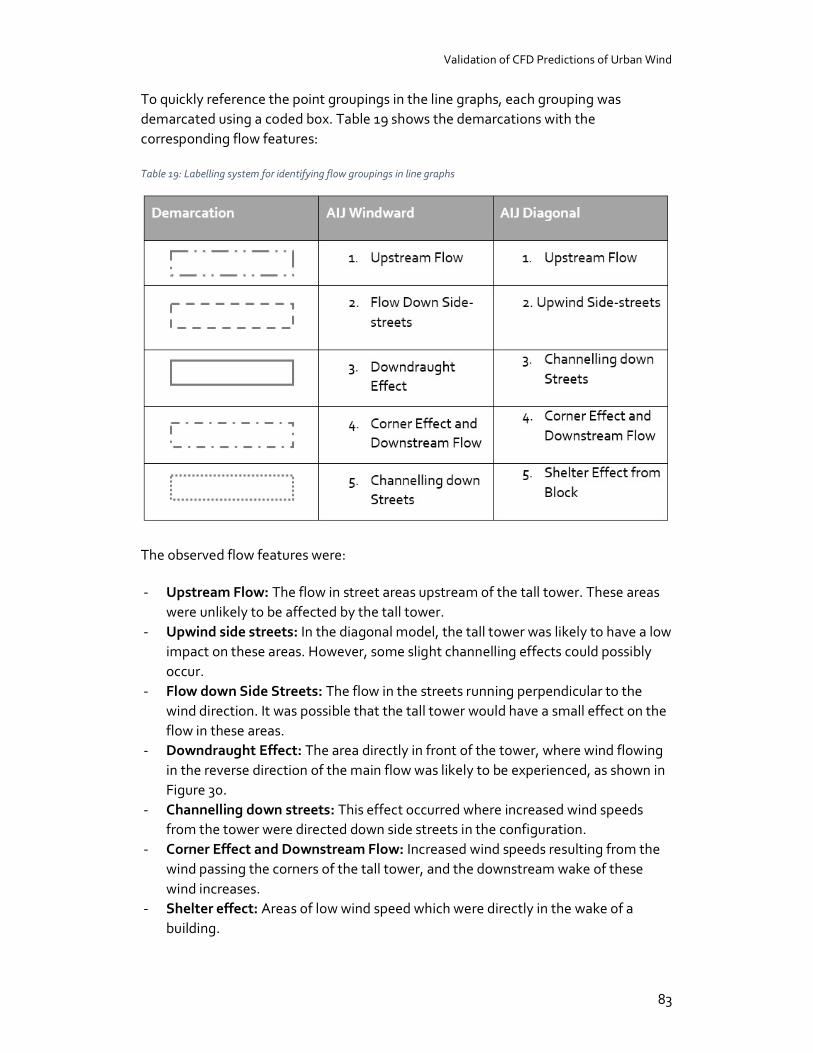
Validation of CFD Predictions of Urban Wind
83
To quickly reference the point groupings in the line graphs, each grouping was demarcated using a coded box. Table 19 shows the demarcations with the corresponding flow features:
Table 19: Labelling system for identifying flow groupings in line graphs
The observed flow features were:
- Upstream Flow: The flow in street areas upstream of the tall tower. These areas were unlikely to be affected by the tall tower.
- Upwind side streets: In the diagonal model, the tall tower was likely to have a low impact on these areas. However, some slight channelling effects could possibly occur.
- Flow down Side Streets: The flow in the streets running perpendicular to the wind direction. It was possible that the tall tower would have a small effect on the flow in these areas.
- Downdraught Effect: The area directly in front of the tower, where wind flowing in the reverse direction of the main flow was likely to be experienced, as shown in Figure 30.
- Channelling down streets: This effect occurred where increased wind speeds from the tower were directed down side streets in the configuration.
- Corner Effect and Downstream Flow: Increased wind speeds resulting from the wind passing the corners of the tall tower, and the downstream wake of these wind increases.
- Shelter effect: Areas of low wind speed which were directly in the wake of a building.
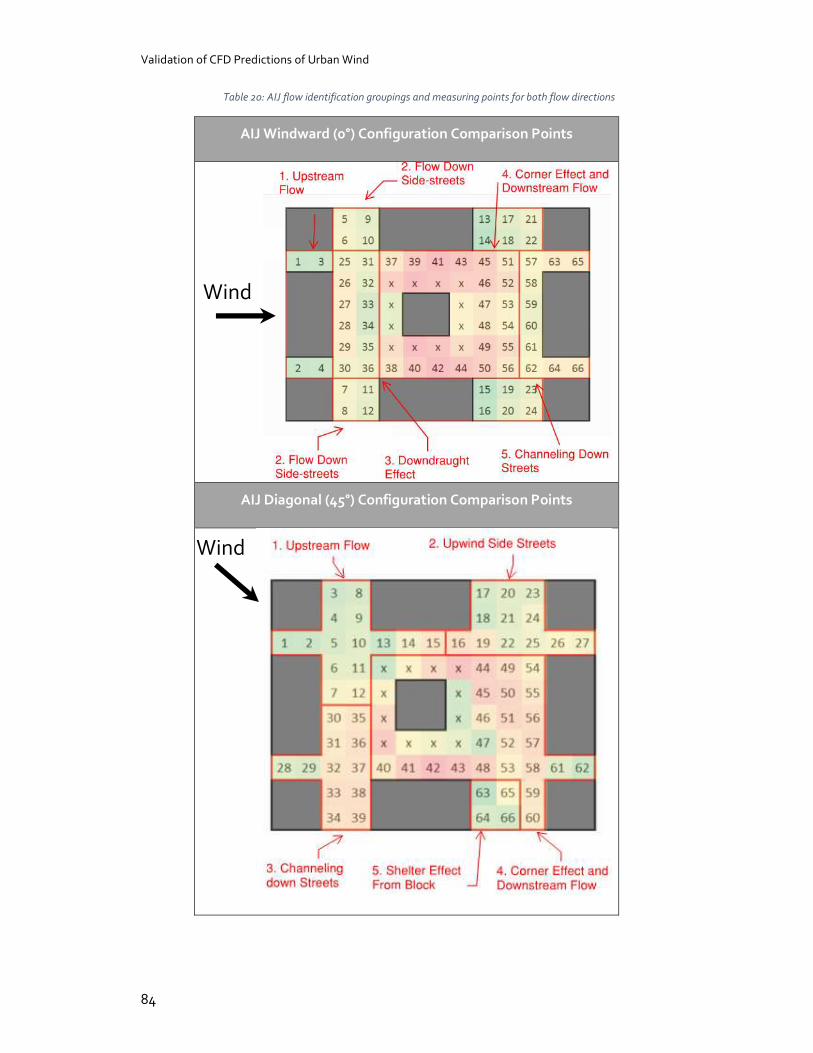
Validation of CFD Predictions of Urban Wind
84
Table 20: AIJ flow identification groupings and measuring points for both flow directions
AIJ Windward (0°) Configuration Comparison Points
AIJ Diagonal (45°) Configuration Comparison Points
Wind
Wind
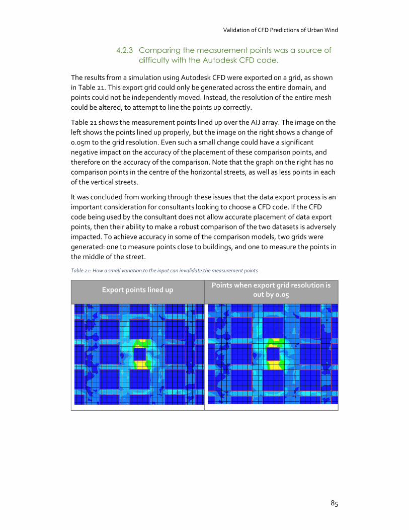
Validation of CFD Predictions of Urban Wind
85
4.2.3 Comparing the measurement points was a source of difficulty with the Autodesk CFD code.
The results from a simulation using Autodesk CFD were exported on a grid, as shown in Table 21. This export grid could only be generated across the entire domain, and points could not be independently moved. Instead, the resolution of the entire mesh could be altered, to attempt to line the points up correctly.
Table 21 shows the measurement points lined up over the AIJ array. The image on the left shows the points lined up properly, but the image on the right shows a change of 0.05m to the grid resolution. Even such a small change could have a significant negative impact on the accuracy of the placement of these comparison points, and therefore on the accuracy of the comparison. Note that the graph on the right has no comparison points in the centre of the horizontal streets, as well as less points in each of the vertical streets.
It was concluded from working through these issues that the data export process is an important consideration for consultants looking to choose a CFD code. If the CFD code being used by the consultant does not allow accurate placement of data export points, then their ability to make a robust comparison of the two datasets is adversely impacted. To achieve accuracy in some of the comparison models, two grids were generated: one to measure points close to buildings, and one to measure the points in the middle of the street.
Table 21: How a small variation to the input can invalidate the measurement points
Export points lined up Points when export grid resolution is out by 0.05

Validation of CFD Predictions of Urban Wind
86
4.2.4 Mesh resolution has a notable impact on the results Figure 28 and Figure 28: AIJ 0° Comparison line graph (top) and scatter plots for 0.2, 0.25 and 0.15 mesh resolutions (bottom)
show the effect of increased resolution of the mesh size for the AIJ configuration at 45° and 0° wind directions. Both graphs show the comparison of wind speed predictions by 5 different mesh resolutions, compared to the wind tunnel measurements recorded by the AIJ, which is denoted by the dashed green line. Each CFD model is denoted by a coloured line.
The agreement between the wind tunnel and CFD is not as good for the tall tower array as for the 2:1:1 block model. This is shown in two ways: the first is that there is a large gap between the wind tunnel measurements and the CFD predictions, for most flow features. This shows that the CFD models under-predicted the measured wind speeds. Two exceptions from this pattern were the side street flows in the windward graph- in particular points 16-30 and the upstream area in the diagonal graph.
The other factor is the shape of the line graphs. The CFD graphs mostly matched the shape of the wind tunnel graph in the windward direction, which suggests that the right flow features were being modelled, even if the magnitude of the wind speed was not accurate. The one exception to this was the downdraught area, where the CFD graphs moved in the opposite direction to the wind tunnel measurements. However, in the diagonal direction, the CFD models did not show the peaks in the wind tunnel graphs for both the channelling area, and the side street upwind of the tower. This suggests that the measured acceleration in these areas was not modelled by the CFD program.
In the diagonal wind direction line graph, the Automatic and 0.5 mesh resolutions significantly underestimate the flow speeds in the corner effect flow area- particularly at points 41-44. Because of this inaccuracy, both mesh resolutions were discounted from further analysis. The scatter plots were used to determine which of the 0.25, 0.2 and 0.15 mesh resolutions best recreated the wind tunnel results. In the 45° direction, the distribution and spread of points for all 3 resolutions was similar. This suggests that the 0.25 mesh resolution was the most appropriate, as it gave similar results to the next finest resolution, at 13 million fewer calculation points.
However, in the 0° scatter graph, the 0.25 mesh shows a different grouping to the 0.2 and 0.15 meshes. The graphs for the 0.2 and 0.15 meshes both contain a cluster of points along the grey line, indicating good agreement between the CFD and wind tunnel measurements. The 0.25 model does not contain a cluster like this, and therefore is not sufficiently accurate to be used.
From these observations, the 0.2 mesh resolution was selected as the best balance between simulation complexity and accuracy. The finer 0.15 resolution did not provide significantly more accurate results, and required 51 million more calculation points to do so. The results of the 0.25 scatter plot suggest that it requires less computing

Validation of CFD Predictions of Urban Wind
87
power, the results it provides are consistently accurate enough to be considered appropriate for the simulation.
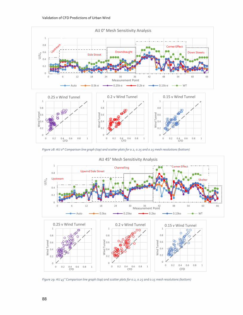
Validation of CFD Predictions of Urban Wind
88
Figure 28: AIJ 0° Comparison line graph (top) and scatter plots for 0.2, 0.25 and 0.15 mesh resolutions (bottom)
Figure 29: AIJ 45° Comparison line graph (top) and scatter plots for 0.2, 0.25 and 0.15 mesh resolutions (bottom)
0
0.2
0.4
0.6
0.8
1
0 6 12 18 24 30 36 42 48 54 60 66
U/U
H
Measurement Point
AIJ 0° Mesh Sensitivity Analysis
Auto 0.5k-e 0.25k-e 0.2k-e 0.15k-e WT
0
0.2
0.4
0.6
0.8
1
0 0.2 0.4 0.6 0.8 1
Win
d Tu
nnel
CFD
0.25 v Wind Tunnel
0
0.2
0.4
0.6
0.8
1
0 0.2 0.4 0.6 0.8 1
Win
d Tu
nnel
CFD
0.2 v Wind Tunnel
0
0.2
0.4
0.6
0.8
1
0 0.2 0.4 0.6 0.8 1
Win
d Tu
nnel
CFD
0.15 v Wind Tunnel
0
0.2
0.4
0.6
0.8
1
0 6 12 18 24 30 36 42 48 54 60 66
U/U
H
Measurement Point
AIJ 45° Mesh Sensitivity Analysis
Auto 0.5ke 0.25ke 0.2ke 0.15ke WT
0
0.2
0.4
0.6
0.8
1
0 0.2 0.4 0.6 0.8 1
Win
d Tu
nnel
CFD
0.25 v Wind Tunnel
0
0.2
0.4
0.6
0.8
1
0 0.2 0.4 0.6 0.8 1
Win
d Tu
nnel
CFD
0.2 v Wind Tunnel
0
0.2
0.4
0.6
0.8
1
0 0.2 0.4 0.6 0.8 1
Win
d Tu
nnel
CFD
0.15 v Wind Tunnel
Downdraught Side Street
Corner Effect
Down Streets
Upstream
Upwind Side Street Channelling Corner Effect
Shelter
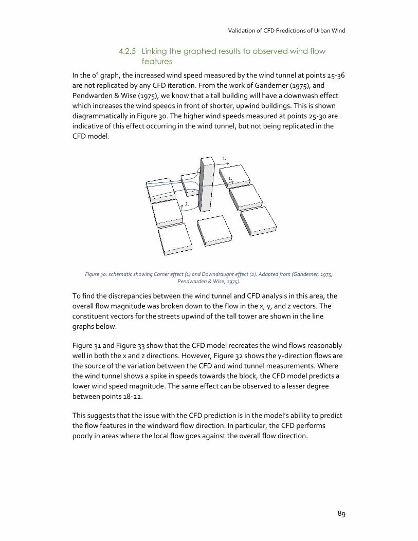
Validation of CFD Predictions of Urban Wind
89
4.2.5 Linking the graphed results to observed wind flow features
In the 0° graph, the increased wind speed measured by the wind tunnel at points 25-36 are not replicated by any CFD iteration. From the work of Gandemer (1975), and Pendwarden & Wise (1975), we know that a tall building will have a downwash effect which increases the wind speeds in front of shorter, upwind buildings. This is shown diagrammatically in Figure 30. The higher wind speeds measured at points 25-30 are indicative of this effect occurring in the wind tunnel, but not being replicated in the CFD model.
Figure 30: schematic showing Corner effect (1) and Downdraught effect (2). Adapted from (Gandemer, 1975; Pendwarden & Wise, 1975).
To find the discrepancies between the wind tunnel and CFD analysis in this area, the overall flow magnitude was broken down to the flow in the x, y, and z vectors. The constituent vectors for the streets upwind of the tall tower are shown in the line graphs below.
Figure 31 and Figure 33 show that the CFD model recreates the wind flows reasonably well in both the x and z directions. However, Figure 32 shows the y-direction flows are the source of the variation between the CFD and wind tunnel measurements. Where the wind tunnel shows a spike in speeds towards the block, the CFD model predicts a lower wind speed magnitude. The same effect can be observed to a lesser degree between points 18-22.
This suggests that the issue with the CFD prediction is in the model’s ability to predict the flow features in the windward flow direction. In particular, the CFD performs poorly in areas where the local flow goes against the overall flow direction.
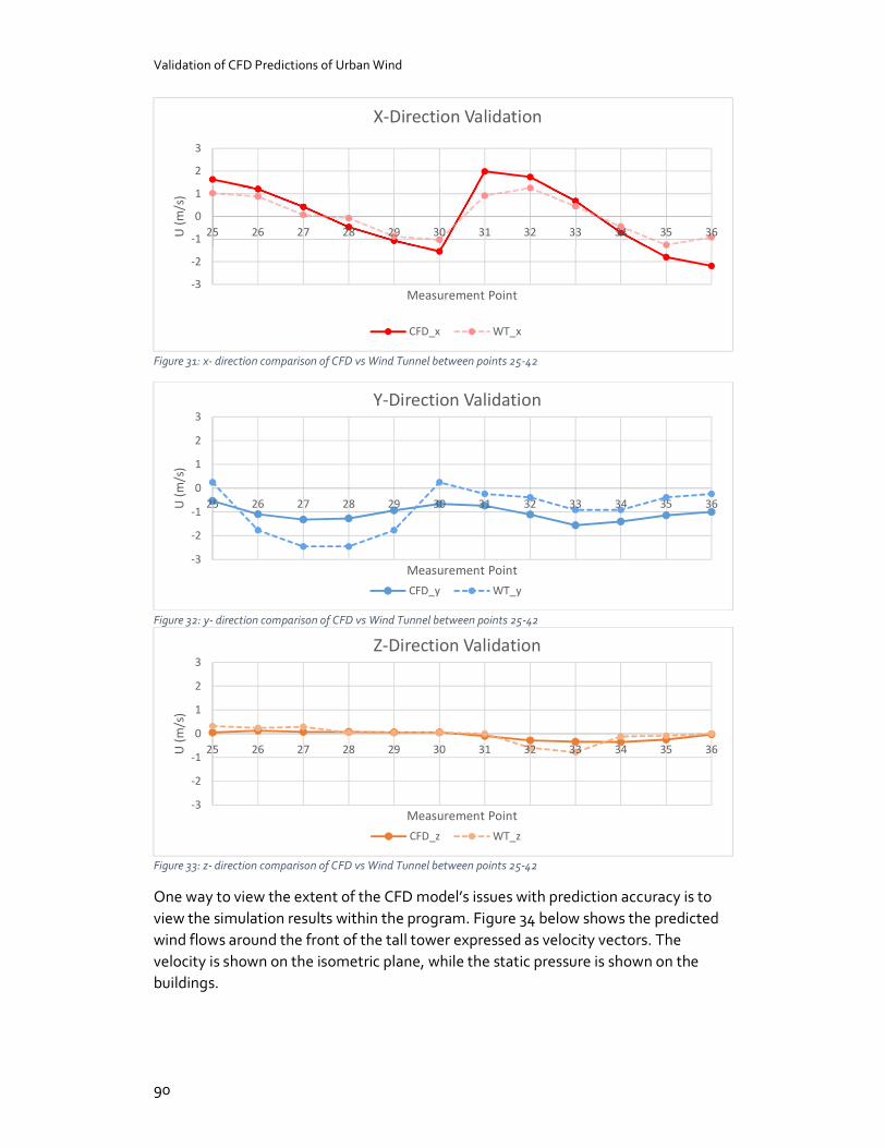
Validation of CFD Predictions of Urban Wind
90
Figure 31: x- direction comparison of CFD vs Wind Tunnel between points 25-42
Figure 32: y- direction comparison of CFD vs Wind Tunnel between points 25-42
Figure 33: z- direction comparison of CFD vs Wind Tunnel between points 25-42
One way to view the extent of the CFD model’s issues with prediction accuracy is to view the simulation results within the program. Figure 34 below shows the predicted wind flows around the front of the tall tower expressed as velocity vectors. The velocity is shown on the isometric plane, while the static pressure is shown on the buildings.
-3
-2
-1
0
1
2
3
25 26 27 28 29 30 31 32 33 34 35 36U (m
/s)
Measurement Point
X-Direction Validation
CFD_x WT_x
-3
-2
-1
0
1
2
3
25 26 27 28 29 30 31 32 33 34 35 36U (m
/s)
Measurement Point
Y-Direction Validation
CFD_y WT_y
-3
-2
-1
0
1
2
3
25 26 27 28 29 30 31 32 33 34 35 36U (m
/s)
Measurement Point
Z-Direction Validation
CFD_z WT_z
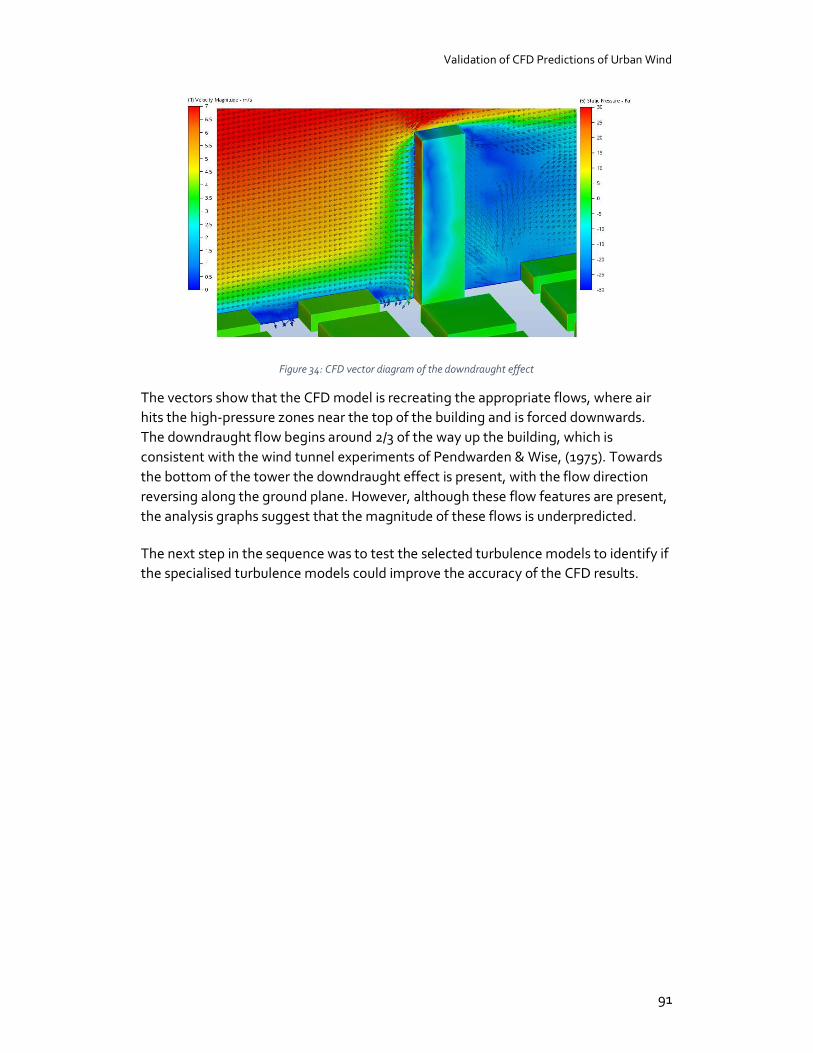
Validation of CFD Predictions of Urban Wind
91
Figure 34: CFD vector diagram of the downdraught effect
The vectors show that the CFD model is recreating the appropriate flows, where air hits the high-pressure zones near the top of the building and is forced downwards. The downdraught flow begins around 2/3 of the way up the building, which is consistent with the wind tunnel experiments of Pendwarden & Wise, (1975). Towards the bottom of the tower the downdraught effect is present, with the flow direction reversing along the ground plane. However, although these flow features are present, the analysis graphs suggest that the magnitude of these flows is underpredicted.
The next step in the sequence was to test the selected turbulence models to identify if the specialised turbulence models could improve the accuracy of the CFD results.
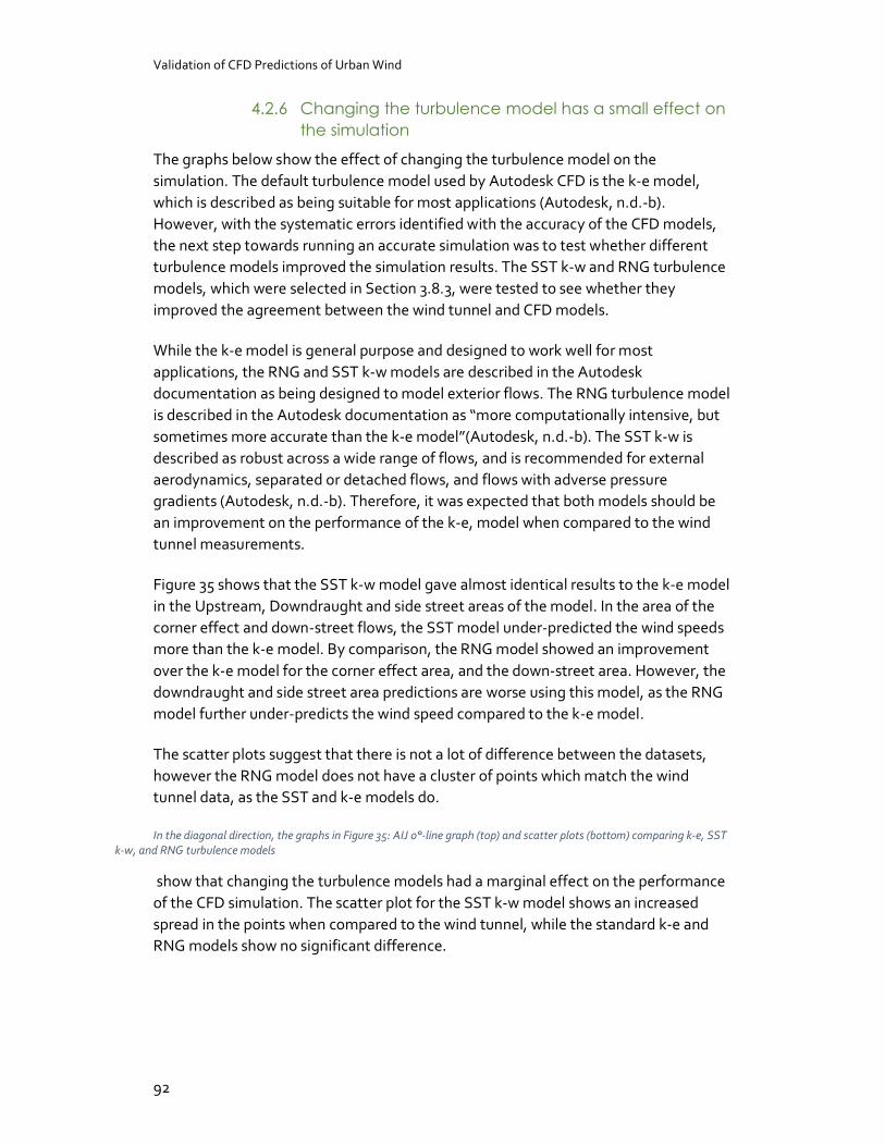
Validation of CFD Predictions of Urban Wind
92
4.2.6 Changing the turbulence model has a small effect on the simulation
The graphs below show the effect of changing the turbulence model on the simulation. The default turbulence model used by Autodesk CFD is the k-e model, which is described as being suitable for most applications (Autodesk, n.d.-b). However, with the systematic errors identified with the accuracy of the CFD models, the next step towards running an accurate simulation was to test whether different turbulence models improved the simulation results. The SST k-w and RNG turbulence models, which were selected in Section 3.8.3, were tested to see whether they improved the agreement between the wind tunnel and CFD models.
While the k-e model is general purpose and designed to work well for most applications, the RNG and SST k-w models are described in the Autodesk documentation as being designed to model exterior flows. The RNG turbulence model is described in the Autodesk documentation as “more computationally intensive, but sometimes more accurate than the k-e model”(Autodesk, n.d.-b). The SST k-w is described as robust across a wide range of flows, and is recommended for external aerodynamics, separated or detached flows, and flows with adverse pressure gradients (Autodesk, n.d.-b). Therefore, it was expected that both models should be an improvement on the performance of the k-e, model when compared to the wind tunnel measurements.
Figure 35 shows that the SST k-w model gave almost identical results to the k-e model in the Upstream, Downdraught and side street areas of the model. In the area of the corner effect and down-street flows, the SST model under-predicted the wind speeds more than the k-e model. By comparison, the RNG model showed an improvement over the k-e model for the corner effect area, and the down-street area. However, the downdraught and side street area predictions are worse using this model, as the RNG model further under-predicts the wind speed compared to the k-e model.
The scatter plots suggest that there is not a lot of difference between the datasets, however the RNG model does not have a cluster of points which match the wind tunnel data, as the SST and k-e models do.
In the diagonal direction, the graphs in Figure 35: AIJ 0°-line graph (top) and scatter plots (bottom) comparing k-e, SST k-w, and RNG turbulence models
show that changing the turbulence models had a marginal effect on the performance of the CFD simulation. The scatter plot for the SST k-w model shows an increased spread in the points when compared to the wind tunnel, while the standard k-e and RNG models show no significant difference.
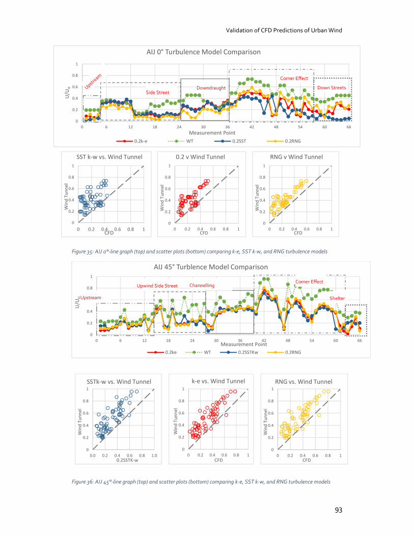
Validation of CFD Predictions of Urban Wind
93
Figure 35: AIJ 0°-line graph (top) and scatter plots (bottom) comparing k-e, SST k-w, and RNG turbulence models
Figure 36: AIJ 45°-line graph (top) and scatter plots (bottom) comparing k-e, SST k-w, and RNG turbulence models
0
0.2
0.4
0.6
0.8
1
0 6 12 18 24 30 36 42 48 54 60 66
U/U
H
Measurement Point
AIJ 0° Turbulence Model Comparison
0.2k-e WT 0.2SST 0.2RNG
0
0.2
0.4
0.6
0.8
1
0 0.2 0.4 0.6 0.8 1
Win
d Tu
nnel
CFD
SST k-w vs. Wind Tunnel
0
0.2
0.4
0.6
0.8
1
0 0.2 0.4 0.6 0.8 1
Win
d Tu
nnel
CFD
0.2 v Wind Tunnel
0
0.2
0.4
0.6
0.8
1
0 0.2 0.4 0.6 0.8 1
Win
d Tu
nnel
CFD
RNG v Wind Tunnel
0
0.2
0.4
0.6
0.8
1
0 6 12 18 24 30 36 42 48 54 60 66
U/U
H
Measurement Point
AIJ 45° Turblence Model Comparison
0.2ke WT 0.2SSTKw 0.2RNG
0
0.2
0.4
0.6
0.8
1
0.0 0.2 0.4 0.6 0.8 1.0
Win
d Tu
nnel
0.2SSTK-w
SSTk-w vs. Wind Tunnel
0
0.2
0.4
0.6
0.8
1
0 0.2 0.4 0.6 0.8 1
Win
d Tu
nnel
CFD
k-e vs. Wind Tunnel
0
0.2
0.4
0.6
0.8
1
0 0.2 0.4 0.6 0.8 1
Win
d Tu
nnel
CFD
RNG vs. Wind Tunnel
Side Street Downdraught
Corner Effect
Down Streets
Upstream
Corner Effect Upwind Side Street Channelling
Shelter
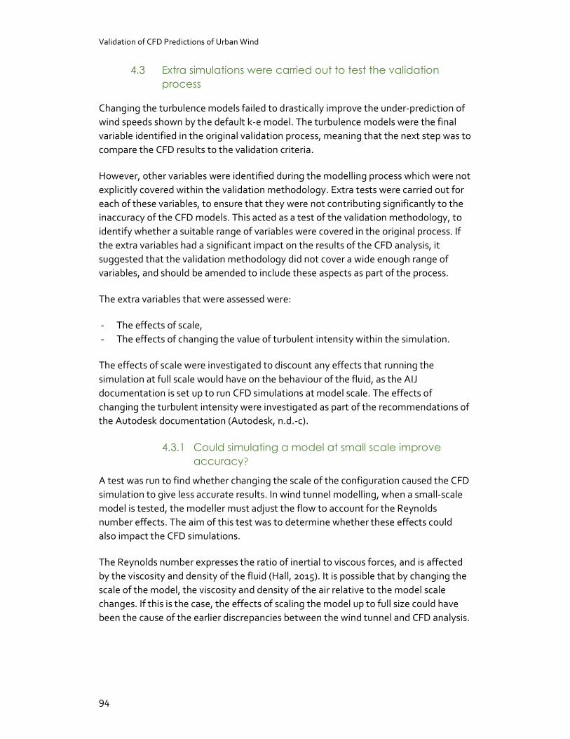
Validation of CFD Predictions of Urban Wind
94
Extra simulations were carried out to test the validation process
Changing the turbulence models failed to drastically improve the under-prediction of wind speeds shown by the default k-e model. The turbulence models were the final variable identified in the original validation process, meaning that the next step was to compare the CFD results to the validation criteria.
However, other variables were identified during the modelling process which were not explicitly covered within the validation methodology. Extra tests were carried out for each of these variables, to ensure that they were not contributing significantly to the inaccuracy of the CFD models. This acted as a test of the validation methodology, to identify whether a suitable range of variables were covered in the original process. If the extra variables had a significant impact on the results of the CFD analysis, it suggested that the validation methodology did not cover a wide enough range of variables, and should be amended to include these aspects as part of the process.
The extra variables that were assessed were:
- The effects of scale, - The effects of changing the value of turbulent intensity within the simulation.
The effects of scale were investigated to discount any effects that running the simulation at full scale would have on the behaviour of the fluid, as the AIJ documentation is set up to run CFD simulations at model scale. The effects of changing the turbulent intensity were investigated as part of the recommendations of the Autodesk documentation (Autodesk, n.d.-c).
4.3.1 Could simulating a model at small scale improve accuracy?
A test was run to find whether changing the scale of the configuration caused the CFD simulation to give less accurate results. In wind tunnel modelling, when a small-scale model is tested, the modeller must adjust the flow to account for the Reynolds number effects. The aim of this test was to determine whether these effects could also impact the CFD simulations.
The Reynolds number expresses the ratio of inertial to viscous forces, and is affected by the viscosity and density of the fluid (Hall, 2015). It is possible that by changing the scale of the model, the viscosity and density of the air relative to the model scale changes. If this is the case, the effects of scaling the model up to full size could have been the cause of the earlier discrepancies between the wind tunnel and CFD analysis.
Validation of CFD Predictions of Urban Wind
95
The test was run for the wind angles of 0° and 45° at the model scale of 1:400. The models had the same proportions, boundary conditions and inlet wind speeds as the full-scale models.
Figure 37 and Figure 38 show that changing the scale did not bring the CFD analysis into line with the wind tunnel tests. In the 0° graph, the small-scale model improves the agreement between the CFD and wind tunnel results in the upstream measurement area. However, it further under-predicts the wind speeds in the side street area, and shows poorer agreement than the full-scale model in the downdraught zone. In the 45° graph, the scaled down model is mostly consistent with the full-size model, apart from in the corner effect zone, where it under-predicted the wind speed.
These tests showed that scale could be discounted as a potential cause of the discrepancies between the CFD simulation and wind tunnel measurements. However, this result is positive for the effectiveness of the validation process as a whole. The minor effects of scale on the CFD results suggest that small-scale validation against wind tunnel models can be trusted for full-scale CFD simulations.
With this option rejected as a cause for the CFD model’s inaccuracy, the final possibility was the effect of the turbulent intensity.
Figure 37: Longitudinal comparison graph, scaled down model
0
0.2
0.4
0.6
0.8
1
0 6 12 18 24 30 36 42 48 54 60 66
U/U
H
Measurement Point
AIJ 0° Scaled Down Model Comparison
0.2k-e WT 0.2SD
Downdraught
Corner Effect
Down Streets Side Street
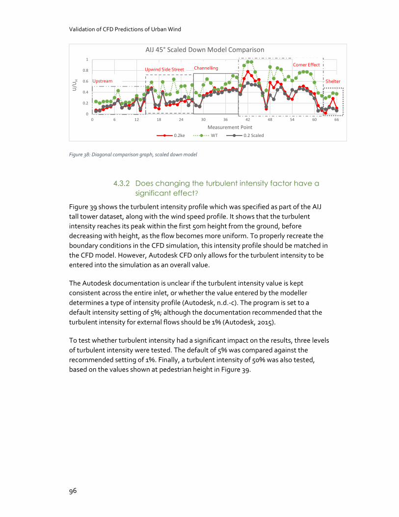
Validation of CFD Predictions of Urban Wind
96
Figure 38: Diagonal comparison graph, scaled down model
4.3.2 Does changing the turbulent intensity factor have a significant effect?
Figure 39 shows the turbulent intensity profile which was specified as part of the AIJ tall tower dataset, along with the wind speed profile. It shows that the turbulent intensity reaches its peak within the first 50m height from the ground, before decreasing with height, as the flow becomes more uniform. To properly recreate the boundary conditions in the CFD simulation, this intensity profile should be matched in the CFD model. However, Autodesk CFD only allows for the turbulent intensity to be entered into the simulation as an overall value.
The Autodesk documentation is unclear if the turbulent intensity value is kept consistent across the entire inlet, or whether the value entered by the modeller determines a type of intensity profile (Autodesk, n.d.-c). The program is set to a default intensity setting of 5%; although the documentation recommended that the turbulent intensity for external flows should be 1% (Autodesk, 2015).
To test whether turbulent intensity had a significant impact on the results, three levels of turbulent intensity were tested. The default of 5% was compared against the recommended setting of 1%. Finally, a turbulent intensity of 50% was also tested, based on the values shown at pedestrian height in Figure 39.
0
0.2
0.4
0.6
0.8
1
0 6 12 18 24 30 36 42 48 54 60 66
U/U
H
Measurement Point
AIJ 45° Scaled Down Model Comparison
0.2ke WT 0.2 Scaled
Channelling
Upstream
Upwind Side Street Corner Effect
Shelter
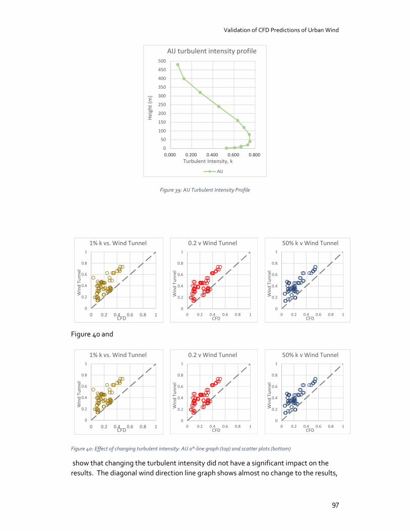
Validation of CFD Predictions of Urban Wind
97
Figure 39: AIJ Turbulent Intensity Profile
Figure 40 and
Figure 40: Effect of changing turbulent intensity: AIJ 0°-line graph (top) and scatter plots (bottom)
show that changing the turbulent intensity did not have a significant impact on the results. The diagonal wind direction line graph shows almost no change to the results,
0
50
100
150
200
250
300
350
400
450
500
0.000 0.200 0.400 0.600 0.800H
eigh
t (m
)
Turbulent Intensity, k
AIJ turbulent intensity profile
AIJ
0
0.2
0.4
0.6
0.8
1
0 0.2 0.4 0.6 0.8 1
Win
d Tu
nnel
CFD
1% k vs. Wind Tunnel
0
0.2
0.4
0.6
0.8
1
0 0.2 0.4 0.6 0.8 1
Win
d Tu
nnel
CFD
0.2 v Wind Tunnel
0
0.2
0.4
0.6
0.8
1
0 0.2 0.4 0.6 0.8 1
Win
d Tu
nnel
CFD
50% k v Wind Tunnel
0
0.2
0.4
0.6
0.8
1
0 0.2 0.4 0.6 0.8 1
Win
d Tu
nnel
CFD
1% k vs. Wind Tunnel
0
0.2
0.4
0.6
0.8
1
0 0.2 0.4 0.6 0.8 1
Win
d Tu
nnel
CFD
0.2 v Wind Tunnel
0
0.2
0.4
0.6
0.8
1
0 0.2 0.4 0.6 0.8 1
Win
d Tu
nnel
CFD
50% k v Wind Tunnel
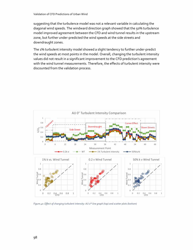
Validation of CFD Predictions of Urban Wind
98
suggesting that the turbulence model was not a relevant variable in calculating the diagonal wind speeds. The windward direction graph showed that the 50% turbulence model improved agreement between the CFD and wind tunnel results in the upstream zone, but further under-predicted the wind speeds at the side streets and downdraught zones.
The 1% turbulent intensity model showed a slight tendency to further under-predict the wind speeds at most points in the model. Overall, changing the turbulent intensity values did not result in a significant improvement to the CFD prediction’s agreement with the wind tunnel measurements. Therefore, the effects of turbulent intensity were discounted from the validation process.
Figure 40: Effect of changing turbulent intensity: AIJ 0°-line graph (top) and scatter plots (bottom)
0
0.2
0.4
0.6
0.8
1
0 6 12 18 24 30 36 42 48 54 60 66
U/U
H
Measurement Point
AIJ 0° Turbulent Intensity Comparison
0.2k-e WT 1% Turbulent Intensity 50%turb
0
0.2
0.4
0.6
0.8
1
0 0.2 0.4 0.6 0.8 1
Win
d Tu
nnel
CFD
1% k vs. Wind Tunnel
0
0.2
0.4
0.6
0.8
1
0 0.2 0.4 0.6 0.8 1
Win
d Tu
nnel
CFD
0.2 v Wind Tunnel
0
0.2
0.4
0.6
0.8
1
0 0.2 0.4 0.6 0.8 1
Win
d Tu
nnel
CFD
50% k v Wind Tunnel
Downdraught Corner Effect
Down Streets Side Street
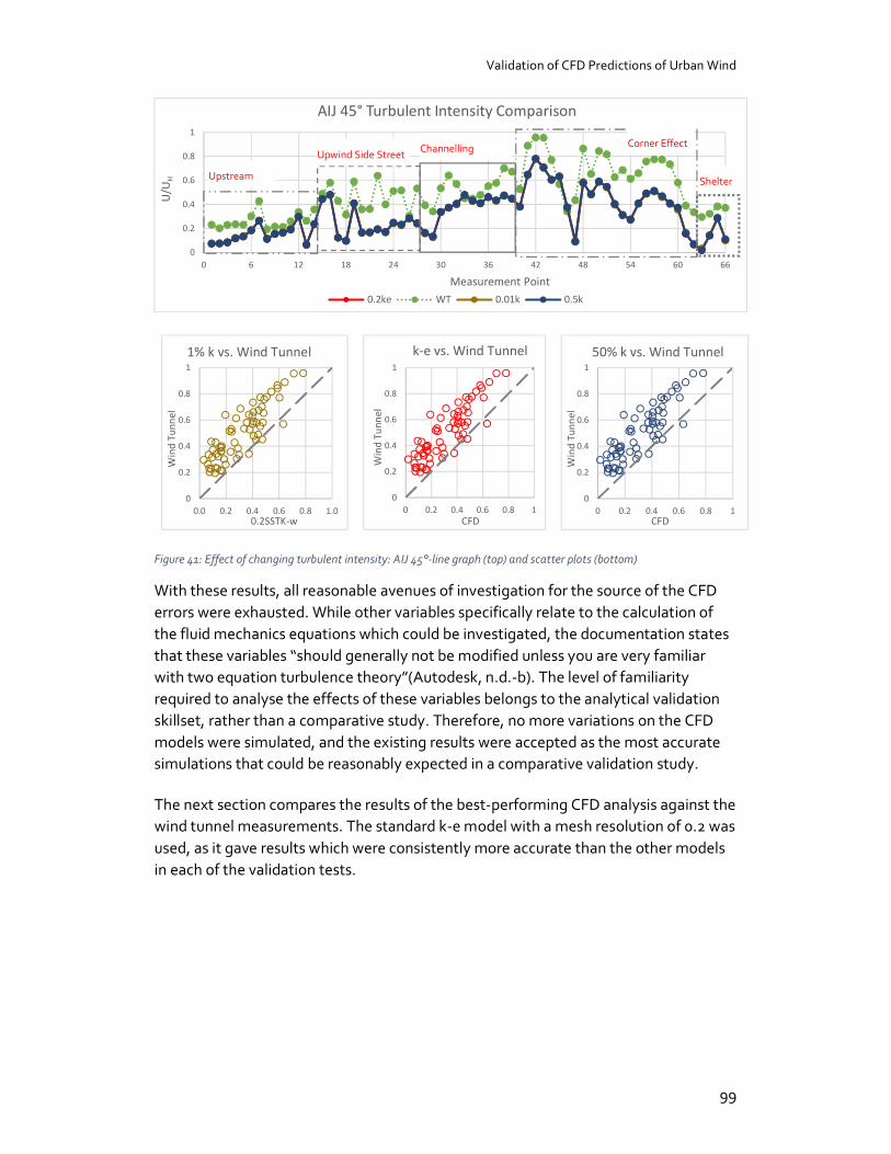
Validation of CFD Predictions of Urban Wind
99
Figure 41: Effect of changing turbulent intensity: AIJ 45°-line graph (top) and scatter plots (bottom)
With these results, all reasonable avenues of investigation for the source of the CFD errors were exhausted. While other variables specifically relate to the calculation of the fluid mechanics equations which could be investigated, the documentation states that these variables “should generally not be modified unless you are very familiar with two equation turbulence theory”(Autodesk, n.d.-b). The level of familiarity required to analyse the effects of these variables belongs to the analytical validation skillset, rather than a comparative study. Therefore, no more variations on the CFD models were simulated, and the existing results were accepted as the most accurate simulations that could be reasonably expected in a comparative validation study.
The next section compares the results of the best-performing CFD analysis against the wind tunnel measurements. The standard k-e model with a mesh resolution of 0.2 was used, as it gave results which were consistently more accurate than the other models in each of the validation tests.
0
0.2
0.4
0.6
0.8
1
0 6 12 18 24 30 36 42 48 54 60 66
U/U
H
Measurement Point
AIJ 45° Turbulent Intensity Comparison
0.2ke WT 0.01k 0.5k
0
0.2
0.4
0.6
0.8
1
0.0 0.2 0.4 0.6 0.8 1.0
Win
d Tu
nnel
0.2SSTK-w
1% k vs. Wind Tunnel
0
0.2
0.4
0.6
0.8
1
0 0.2 0.4 0.6 0.8 1
Win
d Tu
nnel
CFD
k-e vs. Wind Tunnel
0
0.2
0.4
0.6
0.8
1
0 0.2 0.4 0.6 0.8 1
Win
d Tu
nnel
CFD
50% k vs. Wind Tunnel
Channelling Corner Effect
Upstream
Upwind Side Street
Shelter
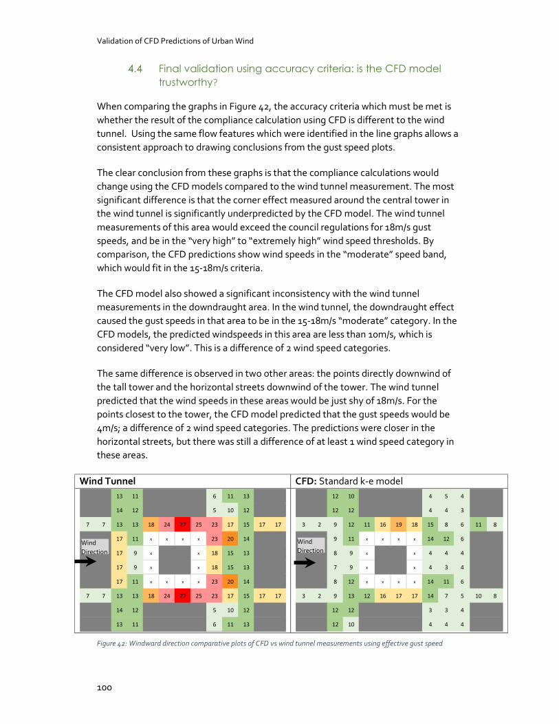
Validation of CFD Predictions of Urban Wind
100
Final validation using accuracy criteria: is the CFD model trustworthy?
When comparing the graphs in Figure 42, the accuracy criteria which must be met is whether the result of the compliance calculation using CFD is different to the wind tunnel. Using the same flow features which were identified in the line graphs allows a consistent approach to drawing conclusions from the gust speed plots.
The clear conclusion from these graphs is that the compliance calculations would change using the CFD models compared to the wind tunnel measurement. The most significant difference is that the corner effect measured around the central tower in the wind tunnel is significantly underpredicted by the CFD model. The wind tunnel measurements of this area would exceed the council regulations for 18m/s gust speeds, and be in the “very high” to “extremely high” wind speed thresholds. By comparison, the CFD predictions show wind speeds in the “moderate” speed band, which would fit in the 15-18m/s criteria.
The CFD model also showed a significant inconsistency with the wind tunnel measurements in the downdraught area. In the wind tunnel, the downdraught effect caused the gust speeds in that area to be in the 15-18m/s “moderate” category. In the CFD models, the predicted windspeeds in this area are less than 10m/s, which is considered “very low”. This is a difference of 2 wind speed categories.
The same difference is observed in two other areas: the points directly downwind of the tall tower and the horizontal streets downwind of the tower. The wind tunnel predicted that the wind speeds in these areas would be just shy of 18m/s. For the points closest to the tower, the CFD model predicted that the gust speeds would be 4m/s; a difference of 2 wind speed categories. The predictions were closer in the horizontal streets, but there was still a difference of at least 1 wind speed category in these areas.
Wind Tunnel CFD: Standard k-e model
Figure 42: Windward direction comparative plots of CFD vs wind tunnel measurements using effective gust speed
13 11 6 11 13
14 12 5 10 12
7 7 13 13 18 24 27 25 23 17 15 17 17
17 11 x x x x 23 20 14
17 9 x x 18 15 13
17 9 x x 18 15 13
17 11 x x x x 23 20 14
7 7 13 13 18 24 27 25 23 17 15 17 17
14 12 5 10 12
13 11 6 11 13
12 10 4 5 4
12 12 4 4 3
3 2 9 12 11 16 19 18 15 8 6 11 8
9 11 x x x x 14 12 6
8 9 x x 4 4 4
7 9 x x 4 3 4
8 12 x x x x 14 11 6
3 2 9 13 12 16 17 17 14 7 5 10 8
12 12 3 3 4
12 10 4 4 4
Wind Direction
Wind Direction
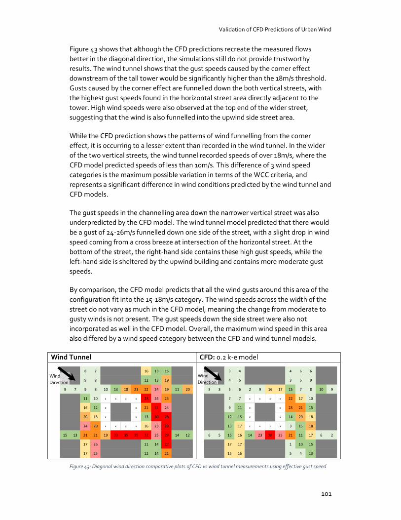
Validation of CFD Predictions of Urban Wind
101
Figure 43 shows that although the CFD predictions recreate the measured flows better in the diagonal direction, the simulations still do not provide trustworthy results. The wind tunnel shows that the gust speeds caused by the corner effect downstream of the tall tower would be significantly higher than the 18m/s threshold. Gusts caused by the corner effect are funnelled down the both vertical streets, with the highest gust speeds found in the horizontal street area directly adjacent to the tower. High wind speeds were also observed at the top end of the wider street, suggesting that the wind is also funnelled into the upwind side street area.
While the CFD prediction shows the patterns of wind funnelling from the corner effect, it is occurring to a lesser extent than recorded in the wind tunnel. In the wider of the two vertical streets, the wind tunnel recorded speeds of over 18m/s, where the CFD model predicted speeds of less than 10m/s. This difference of 3 wind speed categories is the maximum possible variation in terms of the WCC criteria, and represents a significant difference in wind conditions predicted by the wind tunnel and CFD models.
The gust speeds in the channelling area down the narrower vertical street was also underpredicted by the CFD model. The wind tunnel model predicted that there would be a gust of 24-26m/s funnelled down one side of the street, with a slight drop in wind speed coming from a cross breeze at intersection of the horizontal street. At the bottom of the street, the right-hand side contains these high gust speeds, while the left-hand side is sheltered by the upwind building and contains more moderate gust speeds.
By comparison, the CFD model predicts that all the wind gusts around this area of the configuration fit into the 15-18m/s category. The wind speeds across the width of the street do not vary as much in the CFD model, meaning the change from moderate to gusty winds is not present. The gust speeds down the side street were also not incorporated as well in the CFD model. Overall, the maximum wind speed in this area also differed by a wind speed category between the CFD and wind tunnel models.
Wind Tunnel CFD: 0.2 k-e model
Figure 43: Diagonal wind direction comparative plots of CFD vs wind tunnel measurements using effective gust speed
8 7 16 13 15
9 8 12 13 19
9 7 9 8 10 13 18 21 22 24 19 11 20
11 10 x x x x 28 24 23
16 12 x x 21 31 24
20 18 x x 13 30 28
24 20 x x x x 16 23 29
15 13 21 21 19 33 35 35 32 25 29 14 12
17 26 11 14 27
17 25 12 14 21
3 4 4 6 6
4 6 3 6 9
3 3 5 6 2 9 16 17 15 7 8 10 9
7 7 x x x x 22 17 10
9 11 x x 23 21 15
12 15 x x 14 20 18
13 17 x x x x 3 15 18
6 5 15 16 14 23 28 25 21 11 17 6 2
17 17 1 10 15
15 16 5 4 13
Wind Direction
Wind Direction
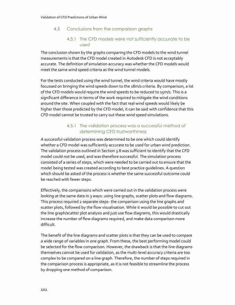
Validation of CFD Predictions of Urban Wind
102
Conclusions from the comparison graphs
4.5.1 The CFD models were not sufficiently accurate to be used
The conclusion shown by the graphs comparing the CFD models to the wind tunnel measurements is that the CFD model created in Autodesk CFD is not acceptably accurate. The definition of simulation accuracy was whether the CFD models would meet the same wind speed criteria as the wind tunnel models.
For the tests conducted using the wind tunnel, the wind criteria would have mostly focussed on bringing the wind speeds down to the 18m/s criteria. By comparison, a lot of the CFD models would require the wind speeds to be reduced to 15m/s. This is a significant difference in terms of the work required to mitigate the wind conditions around the site. When coupled with the fact that real wind speeds would likely be higher than those predicted by the CFD model, it can be said with confidence that this CFD model cannot be trusted to carry out these wind speed simulations.
4.5.1 The validation process was a successful method of determining CFD trustworthiness
A successful validation process was determined to be one which could identify whether a CFD model was sufficiently accurate to be used for urban wind prediction. The validation process outlined in Section 3.8 was sufficient to identify that the CFD model could not be used, and was therefore successful. The simulation process consisted of a series of steps, which were needed to be carried out to ensure that the model being tested was created according to best practice guidelines. A question which should be asked of the process is whether the same successful outcome could be reached with fewer steps.
Effectively, the comparisons which were carried out in the validation process were looking at the same data in 3 ways: using line graphs, scatter plots and flow diagrams. This process required 2 separate steps- the comparison using the line graphs and scatter plots, followed by the flow visualisation. While it would be possible to cut out the line graph/scatter plot analysis and just use flow diagrams, this would drastically increase the number of flow diagrams required, and make data comparison more difficult.
The benefit of the line diagrams and scatter plots is that they can be used to compare a wide range of variables in one graph. From these, the best performing model could be selected for the flow comparison. However, the drawback is that the line diagrams themselves cannot be used for validation, as the multi-level accuracy criteria are too complex to be compared on a line graph. Therefore, the number of steps required in the comparison process is appropriate, as it is not feasible to streamline the process by dropping one method of comparison.
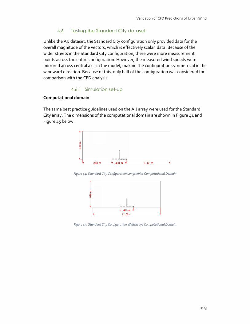
Validation of CFD Predictions of Urban Wind
103
Testing the Standard City dataset
Unlike the AIJ dataset, the Standard City configuration only provided data for the overall magnitude of the vectors, which is effectively scalar data. Because of the wider streets in the Standard City configuration, there were more measurement points across the entire configuration. However, the measured wind speeds were mirrored across central axis in the model, making the configuration symmetrical in the windward direction. Because of this, only half of the configuration was considered for comparison with the CFD analysis.
4.6.1 Simulation set-up
Computational domain
The same best practice guidelines used on the AIJ array were used for the Standard City array. The dimensions of the computational domain are shown in Figure 44 and Figure 45 below:
Figure 44: Standard City Configuration Lengthwise Computational Domain
Figure 45: Standard City Configuration Widthways Computational Domain
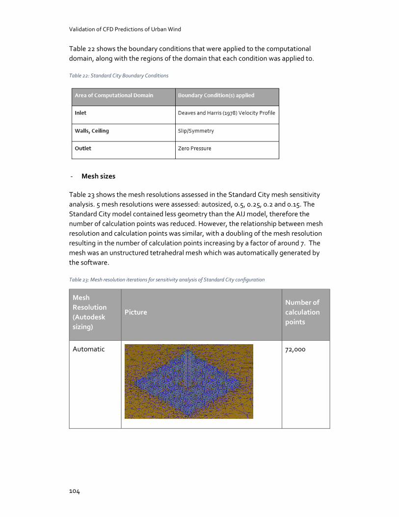
Validation of CFD Predictions of Urban Wind
104
Table 22 shows the boundary conditions that were applied to the computational domain, along with the regions of the domain that each condition was applied to.
Table 22: Standard City Boundary Conditions
- Mesh sizes
Table 23 shows the mesh resolutions assessed in the Standard City mesh sensitivity analysis. 5 mesh resolutions were assessed: autosized, 0.5, 0.25, 0.2 and 0.15. The Standard City model contained less geometry than the AIJ model, therefore the number of calculation points was reduced. However, the relationship between mesh resolution and calculation points was similar, with a doubling of the mesh resolution resulting in the number of calculation points increasing by a factor of around 7. The mesh was an unstructured tetrahedral mesh which was automatically generated by the software.
Table 23: Mesh resolution iterations for sensitivity analysis of Standard City configuration
Mesh Resolution (Autodesk sizing)
Picture Number of calculation points
Automatic
72,000
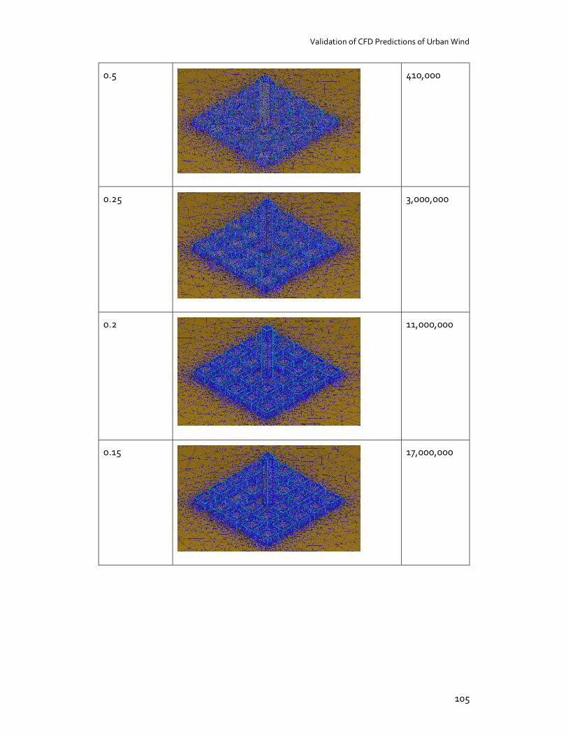
Validation of CFD Predictions of Urban Wind
105
0.5
410,000
0.25
3,000,000
0.2
11,000,000
0.15
17,000,000
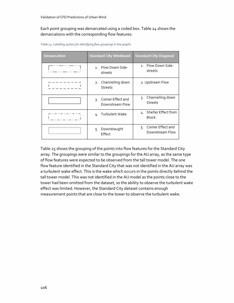
Validation of CFD Predictions of Urban Wind
106
Each point grouping was demarcated using a coded box. Table 24 shows the demarcations with the corresponding flow features:
Table 24: Labelling system for identifying flow groupings in line graphs
Table 25 shows the grouping of the points into flow features for the Standard City array. The groupings were similar to the groupings for the AIJ array, as the same type of flow features were expected to be observed from the tall tower model. The one flow feature identified in the Standard City that was not identified in the AIJ array was a turbulent wake effect. This is the wake which occurs in the points directly behind the tall tower model. This was not identified in the AIJ model as the points close to the tower had been omitted from the dataset, so the ability to observe the turbulent wake effect was limited. However, the Standard City dataset contains enough measurement points that are close to the tower to observe the turbulent wake.
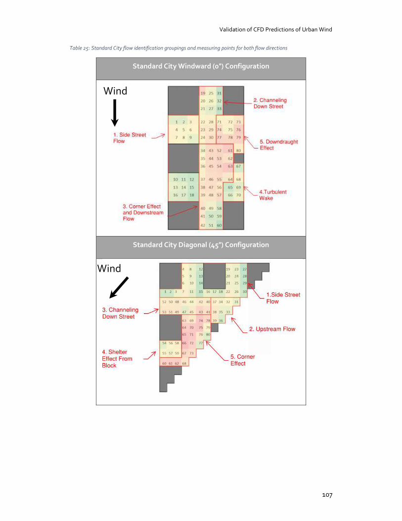
Validation of CFD Predictions of Urban Wind
107
Table 25: Standard City flow identification groupings and measuring points for both flow directions
Standard City Windward (0°) Configuration
Standard City Diagonal (45°) Configuration
Wind
Wind
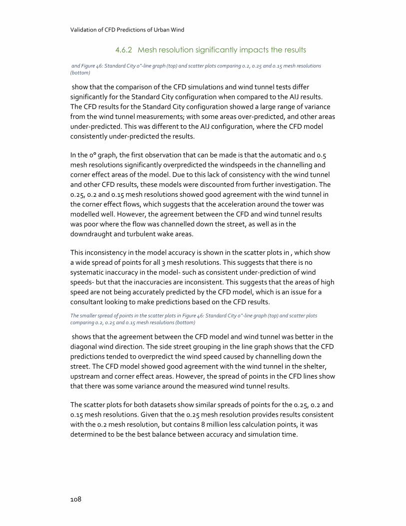
Validation of CFD Predictions of Urban Wind
108
4.6.2 Mesh resolution significantly impacts the results
and Figure 46: Standard City 0°-line graph (top) and scatter plots comparing 0.2, 0.25 and 0.15 mesh resolutions (bottom)
show that the comparison of the CFD simulations and wind tunnel tests differ significantly for the Standard City configuration when compared to the AIJ results. The CFD results for the Standard City configuration showed a large range of variance from the wind tunnel measurements; with some areas over-predicted, and other areas under-predicted. This was different to the AIJ configuration, where the CFD model consistently under-predicted the results.
In the 0° graph, the first observation that can be made is that the automatic and 0.5 mesh resolutions significantly overpredicted the windspeeds in the channelling and corner effect areas of the model. Due to this lack of consistency with the wind tunnel and other CFD results, these models were discounted from further investigation. The 0.25, 0.2 and 0.15 mesh resolutions showed good agreement with the wind tunnel in the corner effect flows, which suggests that the acceleration around the tower was modelled well. However, the agreement between the CFD and wind tunnel results was poor where the flow was channelled down the street, as well as in the downdraught and turbulent wake areas.
This inconsistency in the model accuracy is shown in the scatter plots in , which show a wide spread of points for all 3 mesh resolutions. This suggests that there is no systematic inaccuracy in the model- such as consistent under-prediction of wind speeds- but that the inaccuracies are inconsistent. This suggests that the areas of high speed are not being accurately predicted by the CFD model, which is an issue for a consultant looking to make predictions based on the CFD results.
The smaller spread of points in the scatter plots in Figure 46: Standard City 0°-line graph (top) and scatter plots comparing 0.2, 0.25 and 0.15 mesh resolutions (bottom)
shows that the agreement between the CFD model and wind tunnel was better in the diagonal wind direction. The side street grouping in the line graph shows that the CFD predictions tended to overpredict the wind speed caused by channelling down the street. The CFD model showed good agreement with the wind tunnel in the shelter, upstream and corner effect areas. However, the spread of points in the CFD lines show that there was some variance around the measured wind tunnel results.
The scatter plots for both datasets show similar spreads of points for the 0.25, 0.2 and 0.15 mesh resolutions. Given that the 0.25 mesh resolution provides results consistent with the 0.2 mesh resolution, but contains 8 million less calculation points, it was determined to be the best balance between accuracy and simulation time.
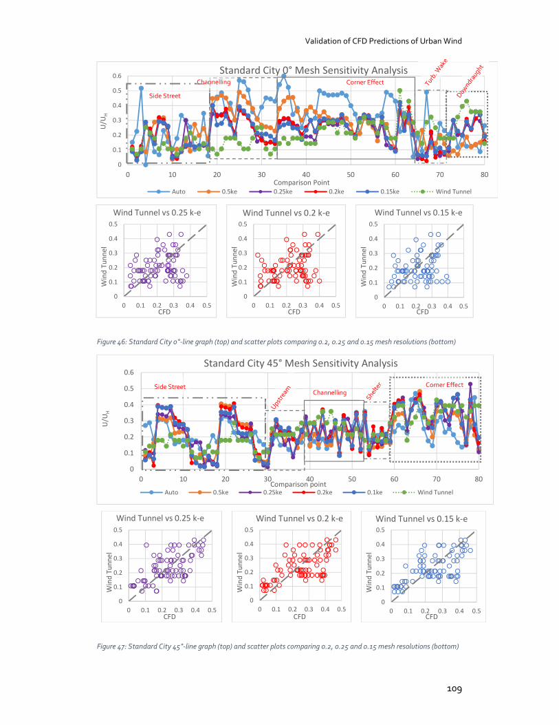
Validation of CFD Predictions of Urban Wind
109
Figure 46: Standard City 0°-line graph (top) and scatter plots comparing 0.2, 0.25 and 0.15 mesh resolutions (bottom)
Figure 47: Standard City 45°-line graph (top) and scatter plots comparing 0.2, 0.25 and 0.15 mesh resolutions (bottom)
0
0.1
0.2
0.3
0.4
0.5
0.6
0 10 20 30 40 50 60 70 80
U/U
H
Comparison Point
Standard City 0° Mesh Sensitivity Analysis
Auto 0.5ke 0.25ke 0.2ke 0.15ke Wind Tunnel
0
0.1
0.2
0.3
0.4
0.5
0 0.1 0.2 0.3 0.4 0.5
Win
d Tu
nnel
CFD
Wind Tunnel vs 0.25 k-e
0
0.1
0.2
0.3
0.4
0.5
0 0.1 0.2 0.3 0.4 0.5
Win
d Tu
nnel
CFD
Wind Tunnel vs 0.2 k-e
0
0.1
0.2
0.3
0.4
0.5
0 0.1 0.2 0.3 0.4 0.5
Win
d Tu
nnel
CFD
Wind Tunnel vs 0.15 k-e
0
0.1
0.2
0.3
0.4
0.5
0.6
0 10 20 30 40 50 60 70 80
U/U
H
Comparison point
Standard City 45° Mesh Sensitivity Analysis
Auto 0.5ke 0.25ke 0.2ke 0.1ke Wind Tunnel
0
0.1
0.2
0.3
0.4
0.5
0 0.1 0.2 0.3 0.4 0.5
Win
d Tu
nnel
CFD
Wind Tunnel vs 0.25 k-e
0
0.1
0.2
0.3
0.4
0.5
0 0.1 0.2 0.3 0.4 0.5
Win
d Tu
nnel
CFD
Wind Tunnel vs 0.2 k-e
0
0.1
0.2
0.3
0.4
0.5
0 0.1 0.2 0.3 0.4 0.5
Win
d Tu
nnel
CFD
Wind Tunnel vs 0.15 k-e
Side Street
Channelling Corner Effect
Side Street Channelling
Corner Effect

Validation of CFD Predictions of Urban Wind
110
4.6.3 Changing the turbulence model has a small but noticeable effect on the results
The correlations shown in the scatter plots in Figure 48 and Figure 48: 0°-line graph (top) and scatter plots (bottom) comparing k-e, SST k-w, and RNG turbulence models
show that the SST k-w model has a narrower spread of points, and shows slightly better agreement with the wind tunnel results than the other two models. In the line graph in Figure 48, the SST and RNG models show better agreement with the wind tunnel than the k-e model, in the downdraught and turbulent wake areas. However, both of these models tend to overpredict the wind speeds caused by the corner effect, while the k-e model shows good agreement with the wind tunnel. In the channelling area, the SST model shows the best agreement with the wind tunnel.
The line graph in Figure 48: 0°-line graph (top) and scatter plots (bottom) comparing k-e, SST k-w, and RNG turbulence models
shows that wind speed in the side street areas are over-predicted by all three CFD models. However, the SST model shows the closest agreement with the wind tunnel. The CFD models predict the upstream, shelter and corner effects relatively well, however each CFD model shows some fluctuation around the wind tunnel results. In the channelling area, the RNG model shows a lot of variation around the wind tunnel graph, suggesting that it does not model the channelling effects well.
Comparing the line graphs suggests that the three turbulence models were relatively consistent in terms of performance, with no one model performing significantly better than the others. However, the scatterplot analysis showed that the SST model predictions consistently showed better agreement with the wind tunnel analysis. Therefore, the SST model was selected for the accuracy criteria comparison.
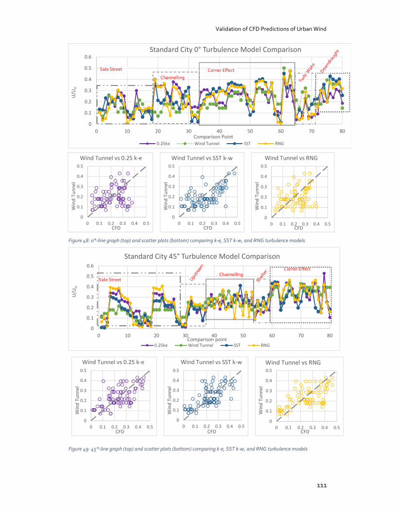
Validation of CFD Predictions of Urban Wind
111
Figure 48: 0°-line graph (top) and scatter plots (bottom) comparing k-e, SST k-w, and RNG turbulence models
Figure 49: 45°-line graph (top) and scatter plots (bottom) comparing k-e, SST k-w, and RNG turbulence models
0
0.1
0.2
0.3
0.4
0.5
0.6
0 10 20 30 40 50 60 70 80
U/U
H
Comparison Point
Standard City 0° Turbulence Model Comparison
0.25ke Wind Tunnel SST RNG
ChannellingCorner EffectSide Street
0
0.1
0.2
0.3
0.4
0.5
0 0.1 0.2 0.3 0.4 0.5
Win
d Tu
nnel
CFD
Wind Tunnel vs 0.25 k-e
0
0.1
0.2
0.3
0.4
0.5
0 0.1 0.2 0.3 0.4 0.5
Win
d Tu
nnel
CFD
Wind Tunnel vs SST k-w
0
0.1
0.2
0.3
0.4
0.5
0 0.1 0.2 0.3 0.4 0.5
Win
d Tu
nnel
CFD
Wind Tunnel vs RNG
0
0.1
0.2
0.3
0.4
0.5
0.6
0 10 20 30 40 50 60 70 80
U/U
H
Comparison point
Standard City 45° Turbulence Model Comparison
0.25ke Wind Tunnel SST RNG
Side StreetChannelling
Corner Effect
0
0.1
0.2
0.3
0.4
0.5
0 0.1 0.2 0.3 0.4 0.5
Win
d Tu
nnel
CFD
Wind Tunnel vs 0.25 k-e
0
0.1
0.2
0.3
0.4
0.5
0 0.1 0.2 0.3 0.4 0.5
Win
d Tu
nnel
CFD
Wind Tunnel vs SST k-w
0
0.1
0.2
0.3
0.4
0.5
0 0.1 0.2 0.3 0.4 0.5
Win
d Tu
nnel
CFD
Wind Tunnel vs RNG

Validation of CFD Predictions of Urban Wind
112
4.6.4 Is a bigger array necessarily better?
One of the concerns raised about the Standard City configuration was the size of the array. The literature review suggested that a 5x5 array did not provide a sufficient area for the flow to fully develop around the tower. The channelling effects noted at the upwind end of the CFD array suggest that the array size did have a significant effect on the results.
Because the array only had 2 rows of blocks upstream of the tower building, the wind was still being channelled from the free flow area past the measurement points. As a result, the wind speed past the measurement points was increased in the CFD models, compared to the wind tunnel measurements. This is shown in the windward graphs, where the CFD models predicted a spike in the wind speed at the points upwind of the tower. When compared to the measurement points for the AIJ tower, this kind of wind channelling was not observed, as the AIJ configuration had a greater number of rows upstream to avoid this type of channelling effect.
Interestingly, the wind tunnel results for the Standard City did not observe this kind of spike in the wind speeds at the upwind points in the tower. The wind tunnel measurements show what could be expected of the flow around this array: no increase in wind speeds at the areas upwind of the block, with increasing speeds around the wake of the building. It is possible that the roughness elements used to create the speed and turbulence profiles created a flow that was well developed and did not channel through the array in the same way.
The channelling effect was not observed to the same extent in the diagonal model, as the wind was not directly channelled into the streets. However, there was a noticeable increase in the wind speeds at the side street flow areas; particularly at points which were at the windward edge of the model and not directly sheltered by a building.
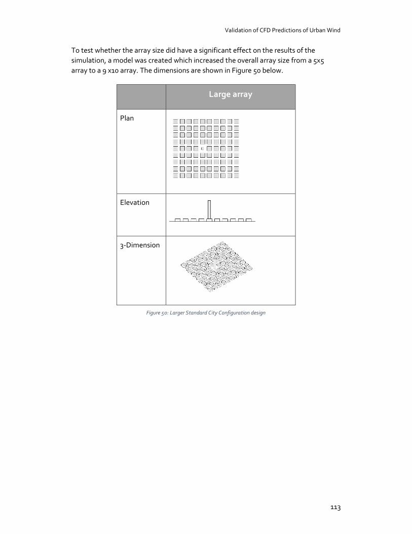
Validation of CFD Predictions of Urban Wind
113
To test whether the array size did have a significant effect on the results of the simulation, a model was created which increased the overall array size from a 5x5 array to a 9 x10 array. The dimensions are shown in Figure 50 below.
Large array
Plan
Elevation
3-Dimension
Figure 50: Larger Standard City Configuration design
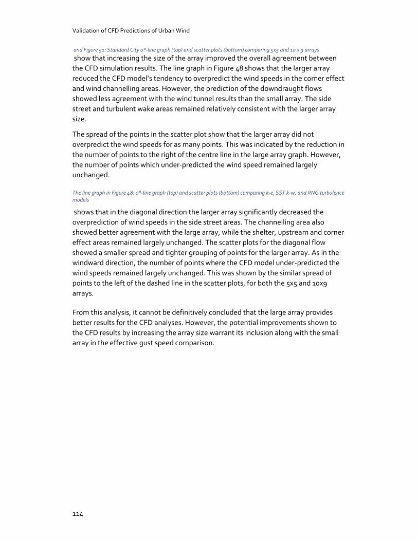
Validation of CFD Predictions of Urban Wind
114
and Figure 51: Standard City 0°-line graph (top) and scatter plots (bottom) comparing 5x5 and 10 x 9 arrays
show that increasing the size of the array improved the overall agreement between the CFD simulation results. The line graph in Figure 48 shows that the larger array reduced the CFD model’s tendency to overpredict the wind speeds in the corner effect and wind channelling areas. However, the prediction of the downdraught flows showed less agreement with the wind tunnel results than the small array. The side street and turbulent wake areas remained relatively consistent with the larger array size.
The spread of the points in the scatter plot show that the larger array did not overpredict the wind speeds for as many points. This was indicated by the reduction in the number of points to the right of the centre line in the large array graph. However, the number of points which under-predicted the wind speed remained largely unchanged.
The line graph in Figure 48: 0°-line graph (top) and scatter plots (bottom) comparing k-e, SST k-w, and RNG turbulence models
shows that in the diagonal direction the larger array significantly decreased the overprediction of wind speeds in the side street areas. The channelling area also showed better agreement with the large array, while the shelter, upstream and corner effect areas remained largely unchanged. The scatter plots for the diagonal flow showed a smaller spread and tighter grouping of points for the larger array. As in the windward direction, the number of points where the CFD model under-predicted the wind speeds remained largely unchanged. This was shown by the similar spread of points to the left of the dashed line in the scatter plots, for both the 5x5 and 10x9 arrays.
From this analysis, it cannot be definitively concluded that the large array provides better results for the CFD analyses. However, the potential improvements shown to the CFD results by increasing the array size warrant its inclusion along with the small array in the effective gust speed comparison.
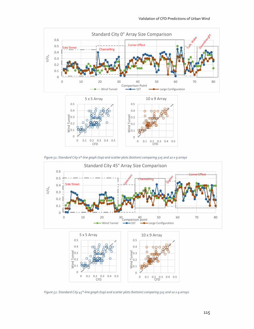
Validation of CFD Predictions of Urban Wind
115
Figure 51: Standard City 0°-line graph (top) and scatter plots (bottom) comparing 5x5 and 10 x 9 arrays
Figure 52: Standard City 45°-line graph (top) and scatter plots (bottom) comparing 5x5 and 10 x 9 arrays
0
0.1
0.2
0.3
0.4
0.5
0.6
0 10 20 30 40 50 60 70 80
U/U
H
Comparison Point
Standard City 0° Array Size Comparison
Wind Tunnel SST Large Configuration
Corner Effect
0
0.1
0.2
0.3
0.4
0.5
0 0.1 0.2 0.3 0.4 0.5
Win
d Tu
nnel
CFD
5 x 5 Array
0
0.1
0.2
0.3
0.4
0.5
0 0.1 0.2 0.3 0.4 0.5
Win
d Tu
nnel
CFD
10 x 9 Array
0
0.1
0.2
0.3
0.4
0.5
0.6
0 10 20 30 40 50 60 70 80
U/U
H
Comparison point
Standard City 45° Array Size Comparison
Wind Tunnel SST Large Configuration
Side Street
ChannellingCorner Effect
0
0.1
0.2
0.3
0.4
0.5
0 0.1 0.2 0.3 0.4 0.5
Win
d Tu
nnel
CFD
5 x 5 Array
0
0.1
0.2
0.3
0.4
0.5
0 0.1 0.2 0.3 0.4 0.5
Win
d Tu
nnel
CFD
10 x 9 Array
Side Street Channelling
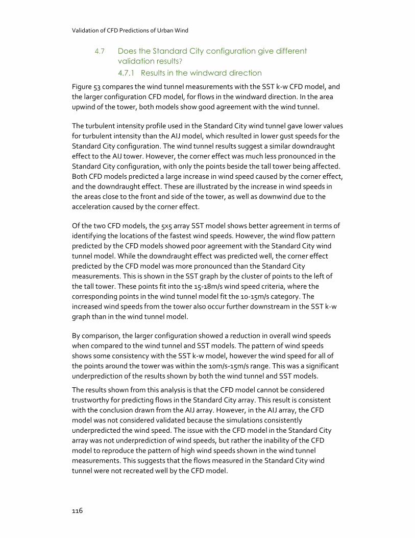
Validation of CFD Predictions of Urban Wind
116
Does the Standard City configuration give different validation results?
4.7.1 Results in the windward direction
Figure 53 compares the wind tunnel measurements with the SST k-w CFD model, and the larger configuration CFD model, for flows in the windward direction. In the area upwind of the tower, both models show good agreement with the wind tunnel.
The turbulent intensity profile used in the Standard City wind tunnel gave lower values for turbulent intensity than the AIJ model, which resulted in lower gust speeds for the Standard City configuration. The wind tunnel results suggest a similar downdraught effect to the AIJ tower. However, the corner effect was much less pronounced in the Standard City configuration, with only the points beside the tall tower being affected. Both CFD models predicted a large increase in wind speed caused by the corner effect, and the downdraught effect. These are illustrated by the increase in wind speeds in the areas close to the front and side of the tower, as well as downwind due to the acceleration caused by the corner effect.
Of the two CFD models, the 5x5 array SST model shows better agreement in terms of identifying the locations of the fastest wind speeds. However, the wind flow pattern predicted by the CFD models showed poor agreement with the Standard City wind tunnel model. While the downdraught effect was predicted well, the corner effect predicted by the CFD model was more pronounced than the Standard City measurements. This is shown in the SST graph by the cluster of points to the left of the tall tower. These points fit into the 15-18m/s wind speed criteria, where the corresponding points in the wind tunnel model fit the 10-15m/s category. The increased wind speeds from the tower also occur further downstream in the SST k-w graph than in the wind tunnel model.
By comparison, the larger configuration showed a reduction in overall wind speeds when compared to the wind tunnel and SST models. The pattern of wind speeds shows some consistency with the SST k-w model, however the wind speed for all of the points around the tower was within the 10m/s-15m/s range. This was a significant underprediction of the results shown by both the wind tunnel and SST models.
The results shown from this analysis is that the CFD model cannot be considered trustworthy for predicting flows in the Standard City array. This result is consistent with the conclusion drawn from the AIJ array. However, in the AIJ array, the CFD model was not considered validated because the simulations consistently underpredicted the wind speed. The issue with the CFD model in the Standard City array was not underprediction of wind speeds, but rather the inability of the CFD model to reproduce the pattern of high wind speeds shown in the wind tunnel measurements. This suggests that the flows measured in the Standard City wind tunnel were not recreated well by the CFD model.
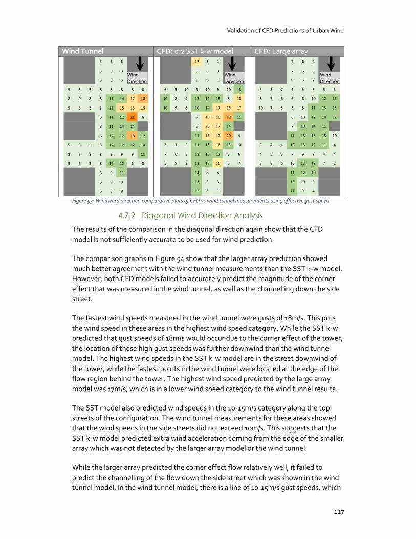
Validation of CFD Predictions of Urban Wind
117
Wind Tunnel CFD: 0.2 SST k-w model CFD: Large array
Figure 53: Windward direction comparative plots of CFD vs wind tunnel measurements using effective gust speed
4.7.2 Diagonal Wind Direction Analysis
The results of the comparison in the diagonal direction again show that the CFD model is not sufficiently accurate to be used for wind prediction.
The comparison graphs in Figure 54 show that the larger array prediction showed much better agreement with the wind tunnel measurements than the SST k-w model. However, both CFD models failed to accurately predict the magnitude of the corner effect that was measured in the wind tunnel, as well as the channelling down the side street.
The fastest wind speeds measured in the wind tunnel were gusts of 18m/s. This puts the wind speed in these areas in the highest wind speed category. While the SST k-w predicted that gust speeds of 18m/s would occur due to the corner effect of the tower, the location of these high gust speeds was further downwind than the wind tunnel model. The highest wind speeds in the SST k-w model are in the street downwind of the tower, while the fastest points in the wind tunnel were located at the edge of the flow region behind the tower. The highest wind speed predicted by the large array model was 17m/s, which is in a lower wind speed category to the wind tunnel results.
The SST model also predicted wind speeds in the 10-15m/s category along the top streets of the configuration. The wind tunnel measurements for these areas showed that the wind speeds in the side streets did not exceed 10m/s. This suggests that the SST k-w model predicted extra wind acceleration coming from the edge of the smaller array which was not detected by the larger array model or the wind tunnel.
While the larger array predicted the corner effect flow relatively well, it failed to predict the channelling of the flow down the side street which was shown in the wind tunnel model. In the wind tunnel model, there is a line of 10-15m/s gust speeds, which
5 6 5
3 5 3
5 5 5
5 3 5 8 8 8 8 8
8 9 8 8 11 14 17 18
5 6 5 8 11 15 15 15
6 11 12 21 6
8 11 14 14
6 12 12 18 12
5 3 5 8 12 12 12 14
8 9 8 8 9 9 9 11
5 6 5 8 12 12 6 8
6 9 11
6 9 8
6 8 8
17 8 1
9 8 3
8 6 1
6 5 10 9 10 9 10 13
10 8 9 12 12 15 8 18
10 9 6 10 14 17 16 17
7 15 16 19 11
9 16 17 14
11 15 17 20 4
5 3 2 11 15 16 13 10
7 6 3 13 15 12 3 6
5 5 2 12 13 16 5 7
14 8 4
13 3 3
12 5 1
7 6 2
7 6 3
9 5 2
5 3 7 9 5 3 5 5
8 7 6 6 6 10 12 13
10 7 3 3 8 11 13 13
3 10 12 14 12
7 13 14 11
11 13 13 15 10
2 4 4 12 13 12 11 4
4 5 3 7 9 2 4 4
3 8 6 10 13 12 7 2
11 12 10
13 10 5
11 9 4
Wind Direction
Wind Direction
Wind Direction
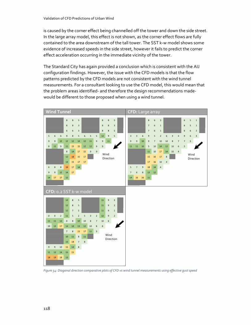
Validation of CFD Predictions of Urban Wind
118
is caused by the corner effect being channelled off the tower and down the side street. In the large array model, this effect is not shown, as the corner effect flows are fully contained to the area downstream of the tall tower. The SST k-w model shows some evidence of increased speeds in the side street, however it fails to predict the corner effect acceleration occurring in the immediate vicinity of the tower.
The Standard City has again provided a conclusion which is consistent with the AIJ configuration findings. However, the issue with the CFD models is that the flow patterns predicted by the CFD models are not consistent with the wind tunnel measurements. For a consultant looking to use the CFD model, this would mean that the problem areas identified- and therefore the design recommendations made- would be different to those proposed when using a wind tunnel.
Wind Tunnel CFD: Large array
CFD: 0.2 SST k-w model
Figure 54: Diagonal direction comparative plots of CFD vs wind tunnel measurements using effective gust speed
8 8 5 8 8 5
8 8 3 8 8 3
6 6 3 8 8 5
5 6 6 9 8 5 6 5 5 12 9 5
9 9 12 12 12 14 12 11 9 9 11
8 11 9 11 15 15 12 12 9 9
8 14 17 15 9 9
12 18 15 17
14 15 17 17
6 8 8 18 17 14
9 9 12 14 17
14 17 17 12
8 6 3 6 5 1
7 6 1 6 5 1
7 6 1 6 6 2
3 3 6 9 5 2 6 4 4 9 6 3
9 9 10 9 7 10 10 8 7 7 5
11 11 10 5 10 14 12 10 6 5
11 10 17 14 10 4
15 16 17 8
17 16 10 4
5 7 9 18 14 4
7 6 8 13 12
14 16 16 11
13 8 5 11 9 3
12 8 5 11 9 2
12 7 2 11 9 1
0 0 2 11 5 2 5 3 2 12 9 2
11 11 12 9 8 10 10 8 7 10 6
10 13 17 14 10 13 12 10 8 8
7 8 15 17 11 3
10 11 8 11
13 18 7 8
9 9 10 15 14 8
11 12 14 15 15
18 19 18 13
Wind Direction
Wind Direction
Wind Direction

Validation of CFD Predictions of Urban Wind
119
Conclusions from the comparison graphs
The evidence shown from the Standard City array comparison leads to the same conclusion as the AIJ configuration: that the CFD models cannot accurately recreate the wind tunnel measurements. Other conclusions were that the wind tunnel results for the windward graph were not in line with the expected results from the flow features described in literature; and that the large array had the opposite effect on the results than expected.
4.8.1 The CFD models created for the test did not meet the accuracy criteria
For the windward test results, the highest wind speed predicted by either CFD model was in the 18-20m/s band. The highest wind speed predicted by the wind tunnel was in the 21-23m/s band. In terms of the WCC criteria, this is no change as both wind speeds would be expected to be reduced to 18m/s. However, using the CFD model would give the impression that a smaller reduction would be acceptable, falling short of what was required.
A more significant problem for the CFD model was that the shape of the predicted flow features varied from what was measured in the wind tunnel. Looking at the CFD model predictions, wind mitigation strategies would focus on reducing high winds downstream of the tower caused by the corner effect. However, the wind tunnel measurements suggest that the corner effect is minimal in comparison to the downdraught effect upwind of the tower, and that this is what should be reduced. Therefore, the design decisions made based on the CFD model would change, and the CFD model is not an acceptable alternative to the wind tunnel measurements.
Although the agreement was better, the same issues exist for the diagonal model. In this case, the CFD models failed to identify the extent of the high wind speed areas, as well as failing to predict the magnitude and location of the highest gust speeds. The wind tunnel results show that the immediate area downstream of the tower would have wind speeds in the 15-18m/s range, including the points directly behind the tower. The CFD model predicted that the points behind the model would have wind speeds of less than 10m/s. Therefore, using the CFD predictions would result in mitigation strategies which only resolve part of the issue, whilst leaving the unsafe wind conditions in other areas.
Another issue is the fact that both CFD models performed poorly for one wind direction, and better in the other. Therefore, neither CFD model can be trusted to provide consistently adequate results.

Validation of CFD Predictions of Urban Wind
120
4.8.2 There were some inconsistencies in the flow features described by the wind tunnel datasets
Both the Standard City and AIJ wind tunnel results show evidence of a downdraught and corner effect causing accelerated wind speeds around the central tower block. These flow features are expected from descriptions provided by Gandemer (1975). However, Gandemer also describes the wake effect, whereby we can expect high wind speeds to continue occurring downstream from a tall building; caused by the acceleration around the edges of the building (1975). The wake effect was present in each CFD model, and in the AIJ wind tunnel measurements; however, it was not recorded in windward Standard City wind tunnel dataset.
This lack of consistency in the modelled flow features occurring in the wind tunnel raises the question of the trustworthiness of the Standard City wind tunnel measurements. The lack of agreement with the other wind tunnel dataset and the relevant literature suggests that the wind tunnel tests should be repeated to produce the same results before they can be considered trustworthy enough for CFD validation.
4.8.3 The channelling effect observed in the smaller array is not necessarily a drawback
From the line and scatter plots, it was expected that the larger configuration would provide better agreement in the windward direction, and have a negligible effect in the diagonal direction. However, the validation graphs showed that the large configuration provided a significant improvement in the diagonal direction, and less agreement in the windward direction.
The lack of agreement in the windward direction shows that increasing the configuration size did not account for differences between the wind tunnel results and the 5x5 array. However, using the larger array in the diagonal direction removed the high windspeeds that were present in the 5x5 array on the perimeter points. This was likely because the wind could develop to an average flow over a larger array. However, the flow in the smaller array was still developing as it reached the measurement points. This meant that the higher wind speeds were being channelled into the measurement points. Further evidence of this is that the larger AIJ array did not have any high wind speeds recorded at the perimeter of the measurement points.
For some city areas, it may be more beneficial to model the effects of wind channelling through a smaller array, as this is a better representation of the existing urban form. This links back to the 5th and final research question of this thesis, as stated in section 1.4 which asked what the requirements of a representative validation suite of wind tunnel tests would be. A conclusion to be drawn from this analysis is that the best method of answering that question is not to prescribe a set configuration
Validation of CFD Predictions of Urban Wind
121
which should be tested, but rather to look at what flow features should be modelled in the wind tunnel for inclusion in a validation suite.
Summary
The results of the CFD analyses have shown that the validation process is able to optimise the CFD process, and identify whether a model is sufficiently accurate to be trusted. The trial run of the test found that the Autodesk CFD models for the AIJ and Standard City arrays were not able to recreate the wind tunnel measurements to a sufficient level of accuracy. This is a successful trial, as the issues and problem areas were identified by the process, rather than a flawed model being trusted.
Both configurations had serious limitations when it came to being used in the validation process. Because the central measurement points are missing, the AIJ configuration uses an incomplete dataset to try and identify flow features in the configuration. This makes comparison difficult, especially for any flow effects which happen close to the tall tower, which would be of interest to a pedestrian wind study.
By comparison, the Standard City array showed a troubling lack of agreement with the other wind tunnel tests, and with the literature on the flow features that should be expected. Therefore, the wind tunnel tests should be repeated and the same results obtained before the dataset can be confidently used for CFD validation.
The conclusion of this analysis is that a new validation configuration should be determined based on the types of flow features which are present in cities. There is a wealth of literature on this topic, which could be used to design appropriate models for wind tunnel testing.
122
5. Conclusions from the CFD Validation Study
The purpose of this thesis was to identify and test a comparative validation process that could quickly determine whether the results of a CFD simulation are trustworthy. The validation process was intended for use by consultants looking to run compliance tests of buildings in urban areas, and it was tested with the Wellington City Council wind speed criteria.
The discussion in this chapter focusses on the discoveries made in carrying out the validation process, and how they relate back to the research questions 1-3. The focus of these questions was whether any validation datasets exist; what the key aspects of those validation datasets would be; and which existing dataset(s) would be the most suitable for validation, based on the key aspects identified in question two. Finally, a set of conclusions is made on the research and development steps that will need to be completed before a validation process which would allow consultants to demonstrate that a CFD model is capable of recreating realistic flow features likely to be found in cities.
What needs to be included in a validation dataset?
The first research question of the thesis asked whether any standardised wind tunnel or full scale datasets existed which are suitable for CFD validation. To answer this question, a focus of the literature survey was a critical evaluation of the existing wind tunnel and full-scale tests carried out in a range of research papers. From this analysis, two datasets were identified as potentially suitable for CFD validation. These were the Architectural Institute of Japan’s data set, and the Standard City dataset used by Cenek, Carpenter, & Jamieson (1992) to represent Wellington city.

Validation of CFD Predictions of Urban Wind
123
5.1.1 The 3D geometry of the dataset is an important consideration
The reason two data sets were used for the validation process- rather than selecting just the best single set- is linked to the second and third research questions. The second research question asked what key aspects of the data sets make them suitable for CFD validation.
The first and most critical key aspect of a dataset was access to data. Of the 29 studies investigated, only five gave access to the wind tunnel data. This significantly narrowed down the scope of available wind tunnel sets.
The second key aspect of a dataset is the ability to model a range of relevant flow features found in urban areas. As discussed in Section 2.2, the ideal validation configuration for a CFD analysis would be a wind tunnel test of the site under investigation, or full scale empirically measured data for the location. However, for most locations, it is unlikely that relevant wind tunnel data for an entire city is available. Similarly, the cost and time requirements of conducting full-scale empirical measurements are such that they are not feasible when compared with the ability to model wind at a small scale. Consequently, wind tunnel tests of generic urban arrays were analysed for their suitability in CFD validation studies.
The purpose of the validation process is to give the modeller confidence that the CFD model being used can accurately predict flow features found on the site under investigation (Blocken et al., 2016). Therefore, a generic validation array should be designed to recreate the types of flow features which are typical of urban areas.
This was the reason for testing two datasets: the AIJ dataset was specifically suited to validating CFD analyses, but the only generic test case provided was the flows occurring around a tall tower in a low-rise city. By comparison, the Standard City data set provided a wider range of flow features to choose from, but the dataset was not specifically designed for CFD validation, and was not as detailed as the AIJ set.
An aspect of the datasets which was identified as important in the literature survey was the array size. The argument made by Tsutsumi, Katayama, & Nishida (1992) was that caution should be taken to not design an array which was too small to allow for city wind flow to become fully developed. The study claimed that any measurements taken within the first 4 rows of an array would not represent the average flow through that array, as the flow features were still developing (Tsutsumi et al., 1992). This was test of a larger array in section 4.8 found that increasing the array size reduced the predicted effects of wind channelling, and created a reduction in overall windspeeds in the array.
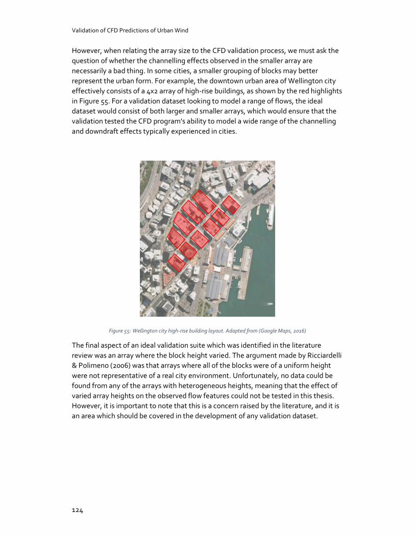
Validation of CFD Predictions of Urban Wind
124
However, when relating the array size to the CFD validation process, we must ask the question of whether the channelling effects observed in the smaller array are necessarily a bad thing. In some cities, a smaller grouping of blocks may better represent the urban form. For example, the downtown urban area of Wellington city effectively consists of a 4x2 array of high-rise buildings, as shown by the red highlights in Figure 55. For a validation dataset looking to model a range of flows, the ideal dataset would consist of both larger and smaller arrays, which would ensure that the validation tested the CFD program's ability to model a wide range of the channelling and downdraft effects typically experienced in cities.
Figure 55: Wellington city high-rise building layout. Adapted from (Google Maps, 2016)
The final aspect of an ideal validation suite which was identified in the literature review was an array where the block height varied. The argument made by Ricciardelli & Polimeno (2006) was that arrays where all of the blocks were of a uniform height were not representative of a real city environment. Unfortunately, no data could be found from any of the arrays with heterogeneous heights, meaning that the effect of varied array heights on the observed flow features could not be tested in this thesis. However, it is important to note that this is a concern raised by the literature, and it is an area which should be covered in the development of any validation dataset.
Validation of CFD Predictions of Urban Wind
125
5.1.2 Comments on the suitability of the Standard City and AIJ configurations as a CFD validation suite.
The third research question asked whether any of the datasets identified in the literature survey was suitable for use as a standard CFD validation dataset. From the requirements discussed above, as well as the conclusions drawn from the validation testing methodology, neither the AIJ nor the Standard City datasets are sufficient as a standardised CFD validation dataset for modelling urban flows. At least one improved dataset is required before a standard CFD validation test of urban flows can be developed. The two datasets used in this thesis are deficient in the following ways:
- The AIJ dataset did not contain enough variation in flow features
While the data provided by the AIJ was of a high quality- and provided good guidance for setting up and running a CFD simulation- only one generic city model was available as part of the AIJ set. This limits the flow features which the array can be used to validate, and means that the array is not suitable for validation of flows in most urban settings. Also, the decision not to include the measurements made in the immediate vicinity of the tower meant that establishing a clear picture of the measured flow features became difficult, which in turn made validating the CFD’s predictions more difficult. However, if these points could be included in the dataset, along with the addition of a larger range of models, the AIJ set could be suitable for the purposes of CFD validation in a range of cities.
- The Standard City dataset also requires more data, the measurements should be checked.
The Standard City dataset was initially preferred over the AIJ dataset, as it gave a wider variety of flow features which could be checked, and therefore could be related to a larger range of urban wind flows. However, while the range of available models was a benefit of the Standard City array, further wind tunnel tests should be carried out to investigate other flow features, such as the effect of heterogenous heights on the observed flow.
Another issue of the Standard City array was that the expected flow features of the tall tower array were not observed. The wake effect, described by Gandemer (1975), was not observed in the Standard City model. This raises the question of how well the wind tunnel measurements could be trusted for the Standard City model. To ensure that the Standard City model is trustworthy, the measurements should be carried out again and compared to ensure consistency with the existing results.
Validation of CFD Predictions of Urban Wind
126
What do the results of the CFD validation test mean?
The fourth research question asked whether the existing guidelines for CFD validation provide adequate guidance for a consultant using CFD to conclude whether they trust the predictions made by a CFD analysis.
The criteria for a successful validation process was whether it could identify that a CFD model was sufficiently accurate to be used for urban wind prediction. In this sense, the validation process was shown to be successful, as it gave consistent results in which showed that the Autodesk CFD models were not suitable for use.
A test of an existing validation process was undertaken which validated 3 urban models in one CFD simulation against existing wind tunnel measurements. The models were: a simple 2:1:1 block which was tested in the Architectural Institute of Japan wind tunnel; a tall tower in a low rise city model, tested in the same wind tunnel; and a tall tower in a low rise city model which was wind tunnel tested by Cenek, Carpenter, & Jamieson (1992). The CFD models of the same configurations were created using Autodesk CFD, and were simulated following best practice guidelines, as well as the recommendations made in the product documentation.
As well as the overall conclusion about the suitability of the CFD code, the following conclusions were made because of the CFD validation test:
5.1.3 Choice of CFD code is an important factor
In section 4.1, Autodesk CFD showed that it was capable of accurately recreating the type of flow features present around a simple 2:1:1 block. However, sections 4.2, and 4.7 found that Autodesk CFD failed to accurately replicate the wind tunnel measurements made in the AIJ city and Standard City models. Therefore, it can be concluded that Autodesk CFD is an example of a code which can accurately recreate the flows found around a simple building, but which requires more work- or at least more guidance- on how to properly set up simulations for complex urban configurations.
Two elements of the CFD code which made the validation process difficult were the data export and inlet conditions specification. To compare the CFD predictions to the wind tunnel measurements, it was important that the points were being compared at the same coordinates on both models. As described in section 3.2, Autodesk CFD’s grid export function was not well suited for this task. Another drawback of the Autodesk CFD software was its inability to model the variation of turbulent intensity with height. The ability to accurately model turbulent intensity is important, as it is a key factor in the calculation of effective gust speeds. Therefore, the ability to only enter one value for turbulent intensity across the entire computational domain seems unreasonable.
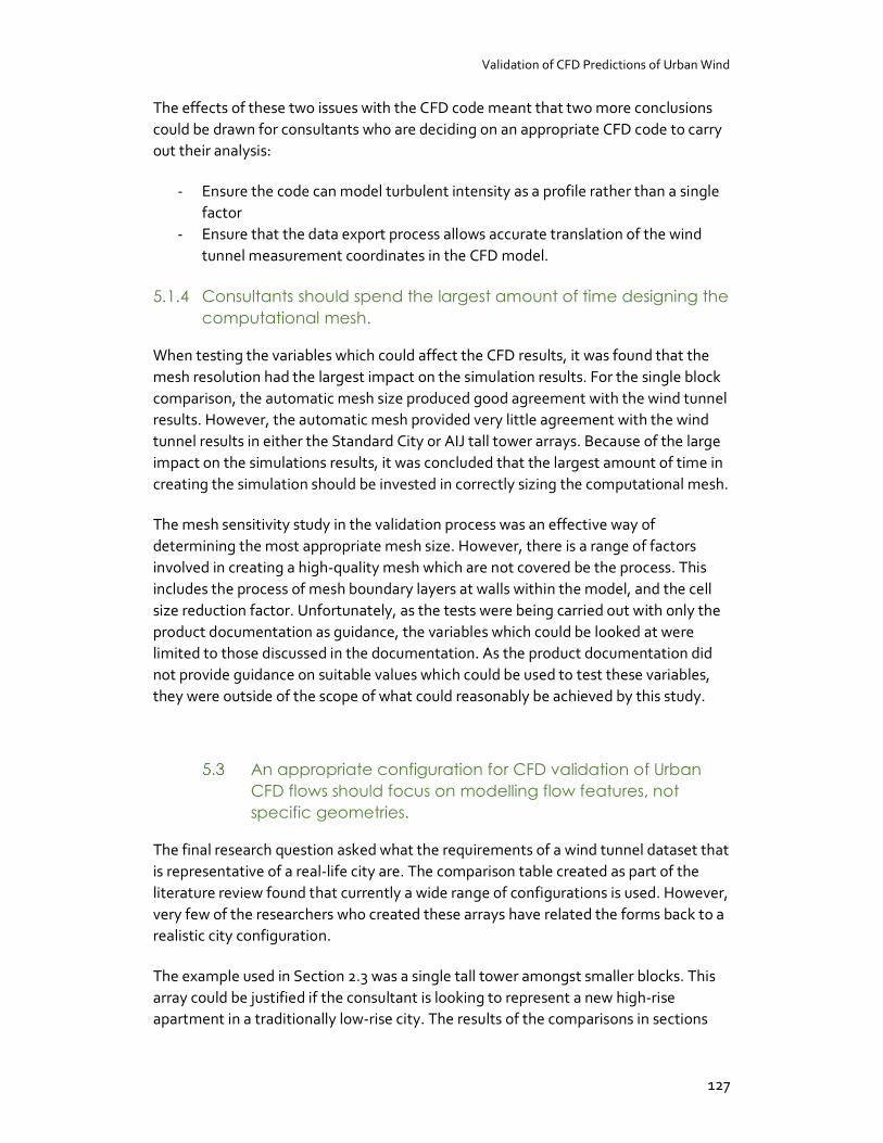
Validation of CFD Predictions of Urban Wind
127
The effects of these two issues with the CFD code meant that two more conclusions could be drawn for consultants who are deciding on an appropriate CFD code to carry out their analysis:
- Ensure the code can model turbulent intensity as a profile rather than a single factor
- Ensure that the data export process allows accurate translation of the wind tunnel measurement coordinates in the CFD model.
5.1.4 Consultants should spend the largest amount of time designing the computational mesh.
When testing the variables which could affect the CFD results, it was found that the mesh resolution had the largest impact on the simulation results. For the single block comparison, the automatic mesh size produced good agreement with the wind tunnel results. However, the automatic mesh provided very little agreement with the wind tunnel results in either the Standard City or AIJ tall tower arrays. Because of the large impact on the simulations results, it was concluded that the largest amount of time in creating the simulation should be invested in correctly sizing the computational mesh.
The mesh sensitivity study in the validation process was an effective way of determining the most appropriate mesh size. However, there is a range of factors involved in creating a high-quality mesh which are not covered be the process. This includes the process of mesh boundary layers at walls within the model, and the cell size reduction factor. Unfortunately, as the tests were being carried out with only the product documentation as guidance, the variables which could be looked at were limited to those discussed in the documentation. As the product documentation did not provide guidance on suitable values which could be used to test these variables, they were outside of the scope of what could reasonably be achieved by this study.
An appropriate configuration for CFD validation of Urban CFD flows should focus on modelling flow features, not specific geometries.
The final research question asked what the requirements of a wind tunnel dataset that is representative of a real-life city are. The comparison table created as part of the literature review found that currently a wide range of configurations is used. However, very few of the researchers who created these arrays have related the forms back to a realistic city configuration.
The example used in Section 2.3 was a single tall tower amongst smaller blocks. This array could be justified if the consultant is looking to represent a new high-rise apartment in a traditionally low-rise city. The results of the comparisons in sections
Validation of CFD Predictions of Urban Wind
128
4.2 and 4.6 found that the flow features in each model were consistently inaccurately predicted by the CFD model. To focus on validating the CFD model’s ability to model flow features, the measurement points were grouped according to the observed flow features in each model. Compared to the point-by-point comparison from the AIJ documentation, these groupings gave a more holistic view than of which flow features the CFD model predicted accurately, and where the CFD model was not accurate.
While the tall tower model could be related to a tall tower in a low rise area, in any city there can be many different building forms, creating many flow features. Therefore, a standard validation dataset must consist of a suite of configurations, which cover the range of flows likely to occur in a city.
A starting point for the development of these flows is the work of Gandemer (1975), which identified a range of typical flow features that occur in cities, and the type of urban geometry which result in these flow features. Figure 56 shows three of the flow regimes identified by Gandemer, to give an idea of the range of flows which could be expected in a truly representative validation suite. By incorporating the flows investigated by Gandemer, the dataset could also be applied to many international cities, giving this research the potential to have a global impact.
Figure 56: Wind effects around buildings. Adapted from (Gandemer, 1975).
Presentation and availability of data are important factors
One of the other results from the literature analysis was the difficulty around access to recorded wind tunnel datasets. If a true standard configuration is to be developed for CFD validation, then one of the aims of the producers should be to allow free access to the data for the conscientious CFD user who wishes to calibrate their own use of a program. This configuration has the potential to become a standard validation set, and therefore public access should be the aim of the producers of the data.
Validation of CFD Predictions of Urban Wind
129
The AIJ approach to this is ideal: to publish the datasets online with a brief description and a guide on how to use the data.
Another strength of the dataset provided by the Architectural Institute of Japan was that the data was presented in a way that was easy to understand and recreate. This allowed for a precise comparison between the wind tunnel and CFD analyses.
Based on the conclusions drawn from carrying out the validation process using these datasets, the minimum requirement for data presentation would be:
- the location of the measurement points should be clearly documented to assist with recreating the model;
- grouping the measurement points numerically into flow regimes.
Finally, for the urban validation set to be universally applicable to CFD users, pressure measurements along the facades of at least one building in the configuration should also be made. Using this data, the CFD models can be validated not just for pedestrian wind speeds, but also for studies which require detailed pressure measurements, such as façade engineering and natural ventilation.
Future incorporation into standards
Once a wind tunnel dataset has been created that matches the criteria listed in the previous section of this chapter, and a process for how to use it has been established and verified, there is the potential for the Wellington City Council to utilise this tool as part of the wind regulations. This could be rolled out in a similar manner to the NEN 8100 wind comfort code, as described by Willemsen & Wisse (2007). In this case, developers can choose between CFD and wind tunnel modelling to identify the effects of new development on urban wind conditions. In the words of Willemsen & Wisse:
“Wind tunnel experiments have a long-standing history of feedback from building practice. CFD is a newcomer and still in the stage that it has to prove itself. It is considered unpractical to exclude the newcomer.”
(Willemsen & Wisse, 2007)
For the CFD measurements to be accepted under the NEN8100 comfort code, a set of quality demands must be met. These include knowledge in the relevant theory behind the CFD code; as well as publishing a quality document which details the CFD code, modelling strategy, and other key assumptions made in the modelling process. Finally, a review document is also prepared for the clients, to ensure transparency within the process (Willemsen & Wisse, 2007). These requirements could support a trustworthy CFD validation process, such as the one outlined in section 3.8, to provide confidence to the user and consenting officer that the CFD predictions can be relied upon.

Validation of CFD Predictions of Urban Wind
130
Further research is required before any regulations concerning the use of CFD can be implemented. This research must focus on testing the methodology determined in this thesis; as well as providing adequate access to the relevant data. However, it is the opinion of the author that with the correct guidance through consultation with the affected parties, CFD modelling could be utilised for pedestrian wind studies in Wellington. If this proves successful, the CFD studies could then also be used not only to improve the urban environment, but also to aid in the design of more energy efficient and comfortable naturally ventilated buildings.
This study has developed and tested a methodology for comparing CFD models to wind tunnel measurements. The results of the validation study successfully identified flaws in the CFD program, which shows that the validation process works as intended. The analysis of existing wind tunnel data sets has provided a framework for future study in this area, with the aim of producing a robust data set for CFD validation, which could be used in as a legal guide for architects and developers.
-finis-
Validation of CFD Predictions of Urban Wind
References 131
References Albrecht, H.-E. (Ed.). (2003). Laser doppler and phase doppler measurement techniques.
Berlin ; New York: Springer.
Architectural Institute of Japan. (2016, September). AIJ Benchmarks for Validation of CFD Simulations Applied to Pedestrian Wind Environment around Buildings.
Aurelius, L. (2011). Project No. 431206: 20 Fenchurch Street (Final Design), London, UK.
Autodesk. (2015, December 28). Two Equation Turbulence Models (TKE & TED) | CFD | Autodesk Knowledge Network. Retrieved 21 March 2017, from https://knowledge.autodesk.com/support/cfd/learn-explore/caas/CloudHelp/cloudhelp/2014/ENU/SimCFD/files/GUID-61C4EB55-362C-48A0-8B22-20F9148D190D-htm.html
Autodesk. (n.d.-a). CFD 2016 Help: Meshing. Retrieved 9 October 2016, from http://help.autodesk.com/view/SCDSE/2016/ENU/?guid=GUID-BE8C3B02-3613-4237-AD18-033FE3002C34
Autodesk. (n.d.-b). CFD 2016 Help: Turbulence. Retrieved 30 October 2016, from http://help.autodesk.com/view/SCDSE/2016/ENU/?guid=GUID-E9E8ACA1-8D49-4A49-8A35-52DB1A2C3E5F
Autodesk. (n.d.-c). CFD 2016 Help: Turbulent Flow. Retrieved 24 October 2016, from http://help.autodesk.com/view/SCDSE/2016/ENU/?guid=GUID-BBA4E008-8346-465B-9FD3-D193CF108AF0
Autodesk. (n.d.-d). Flow Boundary Conditions | CFD | Autodesk Knowledge Network. Retrieved 24 April 2017, from https://knowledge.autodesk.com/support/cfd/learn-explore/caas/CloudHelp/cloudhelp/2018/ENU/SimCFD-UsersGuide/files/GUID-9C1E28D5-B32E-4546-8620-7F428982184A-htm.html
Autodesk. (n.d.-e). Help: Natural Ventilation. Retrieved 15 April 2015, from http://help.autodesk.com/view/SCDSE/2015/ENU/?guid=GUID-F6011744-B69B-47D0-BB2B-50E1BA8DC32D
Autodesk. (n.d.-f). Part Suppression | CFD | Autodesk Knowledge Network. Retrieved 24 April 2017, from https://knowledge.autodesk.com/support/cfd/learn-explore/caas/CloudHelp/cloudhelp/2018/ENU/SimCFD-UsersGuide/files/GUID-C1E20B49-DF2E-45ED-B7F0-BDED8994B8D7-htm.html
Bady, M., Kato, S., & Huang, H. (2008). Towards the application of indoor ventilation efficiency indices to evaluate the air quality of urban areas. Building and Environment, 43(12), 1991–2004. https://doi.org/10.1016/j.buildenv.2007.11.013
Balczo, M., & Eichhorn, J. (2007). Refined Miskam Simulations of the Mock Urban Setting Test. In Model evaluation guidance and protocol document: COST action 732 Quality assurance and improvement of microscale meteorological models. Hamburg: Univ. of Hamburg, Meteorological Inst.
Validation of CFD Predictions of Urban Wind
132
Baskaran, A., & Kashef, A. (1996). Investigation of air flow around buildings using computational fluid dynamics techniques. Engineering Structures, 18(11), 861–875.
Beranek, W. J. (1982). On avoiding wind nuisance around buildings, part 2 (Beperken van windhinder om gebouwen, deel 2). Kluwer Technische Boeken BV.
Biltoft, C. A. (2001). Customer report for mock urban setting test. DPG Document Number 8-CO-160-000-052. Prepared for the Defence Threat Reduction Agency. Retrieved from http://mech.utah.edu/~pardyjak/documents/MUSTCustReport.pdf
Blocken. (2014). 50 years of Computational Wind Engineering: Past, present and future. Journal of Wind Engineering and Industrial Aerodynamics, 129, 69–102. https://doi.org/10.1016/j.jweia.2014.03.008
Blocken. (2015). Computational Fluid Dynamics for urban physics: Importance, scales, possibilities, limitations and ten tips and tricks towards accurate and reliable simulations. Building and Environment, 91, 219–245. https://doi.org/10.1016/j.buildenv.2015.02.015
Blocken, & Carmeliet. (2008). Pedestrian wind conditions at outdoor platforms in a high-rise apartment building: generic sub-configuration validation, wind comfort assessment and uncertainty issues. Wind and Structures, 11(1), 51–70.
Blocken, Carmeliet, J., & Stathopoulos, T. (2007). CFD evaluation of wind speed conditions in passages between parallel buildings—effect of wall-function roughness modifications for the atmospheric boundary layer flow. Journal of Wind Engineering and Industrial Aerodynamics, 95(9–11), 941–962. https://doi.org/10.1016/j.jweia.2007.01.013
Blocken, Janssen, W. D., & van Hooff, T. (2012). CFD simulation for pedestrian wind comfort and wind safety in urban areas: General decision framework and case study for the Eindhoven University campus. Environmental Modelling & Software, 30, 15–34. https://doi.org/10.1016/j.envsoft.2011.11.009
Blocken, Stathopoulos, Carmeliet, J., & Hensen, J. L. M. (2010). Application of computational fluid dynamics in building performance simulation for the outdoor environment: an overview. Journal of Building Performance Simulation, 4(2), 157–184. https://doi.org/10.1080/19401493.2010.513740
Blocken, & Stathopoulos, T. (2013). CFD simulation of pedestrian-level wind conditions around buildings: Past achievements and prospects. Journal of Wind Engineering and Industrial Aerodynamics, 121, 138–145. https://doi.org/10.1016/j.jweia.2013.08.008
Blocken, Stathopoulos, T., & van Beeck, J. P. A. J. (2016). Pedestrian-level wind conditions around buildings: Review of wind-tunnel and CFD techniques and their accuracy for wind comfort assessment. Building and Environment, 100, 50–81. https://doi.org/10.1016/j.buildenv.2016.02.004
Caniot, G., Li, W., & Dupont, G. (2011). Validations and applications of a CFD tool dedicated to wind assessment in urban areas. In 13th International Conference on Wind Engineering. Retrieved from http://meteodyn.com/wp-
Validation of CFD Predictions of Urban Wind
References 133
content/uploads/2012/06/Validations-and-applications-of-a-CFD-tool-dedicated-to-wind-assessment-in-urban-areas.pdf
Carpenter, P. (1988). The Wind Environmet in Wellington City- Full Scale Measurement and Comparison with Wind Tunnel Tests (No. Central Lboratories Report 9-88/1).
Carpenter, P. (2002, October). Wind in city streets.
Carpenter, P. (2016, November 21). Standard City measurement points. Retrieved from https://mail.google.com/mail/u/0/#search/Measurement+points%2C+Paul/15850e1689c89bce
Carpenter, P., Jamieson, N., & Cenek, P. . (1992). The Effect of Architectural Detailing on Pedestrian Level Wind Speeds. Retrieved 4 May 2016, from https://dl.dropboxusercontent.com/content_link/brTY930eI91luqOoLdskEwlCSgeazOtdUy1wGTdzPnJfrMUvahotVbAdnkA6EoLH/file?dl=1
Casey, M., & Wintersgate, T. (Eds.). (2000). ERCOTAC Special Interest Group on ‘Quality and Trust in Industrial CFD’.
Cenek, P. ., Carpenter, P., & Jamieson, N. (1992). The effect of architectural detailing on pedestrian level wind speeds.
Chang, C.-H., & Meroney, R. N. (2001). Numerical and physical modeling of bluff body flow and dispersion in urban street canyons. Journal of Wind Engineering and Industrial Aerodynamics, 89(14), 1325–1334.
Chen, Q. (2009). Ventilation performance prediction for buildings: A method overview and recent applications. Building and Environment, 44(4), 848–858. https://doi.org/10.1016/j.buildenv.2008.05.025
Cheng, H., & Castro, I. P. (2002). Near wall flow over urban-like roughness. Boundary-Layer Meteorology, 104(2), 229–259.
Clark, A. (n.d.). Why is Wellington so windy? Retrieved from http://blog.metservice.com/windy-wellington
Cochran, L., & Derickson, R. (2011). A physical modeler’s view of Computational Wind Engineering. Journal of Wind Engineering and Industrial Aerodynamics, 99(4), 139–153. https://doi.org/10.1016/j.jweia.2011.01.015
Davidson, M. ., Snyder, W. H., Lawson, R. E., & Hunt, J. C. R. (1995). Wind Tunnel Simulation of Plume Dispersion Through Groups of Obstacles. Atmospheric Environment, 30(22), 3715–3731.
Davies, K. (1992). Pedestrian Wind Environment. Retrieved from http://scholarship.law.umt.edu/cgi/viewcontent.cgi?article=1072&context=plrlr
Deaves, D. M., & Harris, R. I. (1978). A Mathematical Model of the Structure of Strong Winds (CIRIA Report No. 76).
Validation of CFD Predictions of Urban Wind
134
Durrani, F., Cook, M. J., & McGuirk, J. J. (2015). Evaluation of LES and RANS CFD modelling of multiple steady states in natural ventilation. Building and Environment, 92, 167–181. https://doi.org/10.1016/j.buildenv.2015.04.027
Evening Post. (1967). Man walking against strong wind, Wellington. Retrieved from https://natlib.govt.nz/records/22739071
Fitzsimons, T. (2011, December 9). How windy is Wellington, really? Stuff.co.nz. Retrieved from http://www.stuff.co.nz/dominion-post/capital-life/6111069/How-windy-is-Wellington-really
Franke, J., Hellsten, A., Schlunzen, H., & Carissimo, B. (Eds.). (2007). Model evaluation guidance and protocol document: COST action 732 Quality assurance and improvement of microscale meteorological models. Hamburg: Univ. of Hamburg, Meteorological Inst.
Frearson, A. (2015, July 23). Walkie Talkie blamed for powerful downdraught on London streets. Retrieved 17 January 2017, from https://www.dezeen.com/2015/07/23/walkie-talkie-skyscraper-rafael-vinoly-blamed-powerful-downdraught-london/
Gandemer, J. (1975). Wind Environment Around Buildings: Aerodynamic Concepts. Proceedings of the Fourth International Conference on Wind Effects on Buildings and Structures, 423–432.
Google Maps. (2016). Wellington City.
Hall, N. (Ed.). (2015, May 5). Similarity Parameters. Retrieved from https://www.grc.nasa.gov/WWW/k-12/airplane/airsim.html
Irwin, P., Denoon, R., & Scott, D. (2013). Wind Tunnel Testing of High-Rise Buildings. Routledge.
Isyumov, N., Helliwell, S., Rosen, S., & Lai, D. (1995). Winds in Cities: effects on Pedestrians and the Dispersion of Ground Level Pollutants. In Wind Climate in Cities (pp. 319–335). Kluwer Academic Publishers.
Jamieson, N., & Brown, D. (1989). Investigation of Measures Available for Improving Ground Level Wind Conditions. Works Consultancy Services.
Jorgenson, F. E. (2002). How to Measure turbulence with hot-wire anemometers- a practical guide. Retrieved from http://web.iitd.ac.in/~pmvs/courses/mel705/hotwire2.pdf
Judkoff, R., Wortman, D., O’Doherty, B., & Burch, J. (2008). Methodology for Validating Building Energy Analysis Simulations (No. NREL/TP-550-42059, 928259). Retrieved from http://www.osti.gov/servlets/purl/928259-CqoQMI/
Kanda, M. (2006). Large-Eddy Simulations on the Effects of Surface Geometry of Building Arrays on Turbulent Organized Structures. Boundary-Layer Meteorology, 118(1), 151–168. https://doi.org/10.1007/s10546-005-5294-2
Karava, P. (2008). Airflow prediction in buildings for natural ventilation design: wind tunnel measurements and simulation.
Ligget, R., & Milne, M. (n.d.). Climate Consultant: Wind Velocity Range.
Validation of CFD Predictions of Urban Wind
References 135
Macdonald, R. W., Griffiths, R. F., & Chea, S. C. (1997). Field Experiments of Dispersion Through regular Arrays of Cubic Structures. Atmospheric Environment, 31(6), 783–795.
Macdonald, R. W., Griffiths, R. F., & Hall, D. J. (1998). A comparison of results from scaled field and wind tunnel modelling of dispersion in arrays of obstacles. Atmospheric Environment, 32(22), 3845–3862.
Mathiesen, K. (2015, October 15). Where is the world’s windiest city? Spoiler alert: it’s not Chicago. Retrieved 21 February 2017, from http://www.theguardian.com/cities/2015/oct/15/where-world-windiest-city-spoiler-alert-chicago-wellington
Meroney, R. (2004). Wind tunnel and numerical simulation of pollution dispersion: a hybrid approach.
Millward-Hopkins, J. T., Tomlin, A. S., Ma, L., Ingham, D., & Pourkashanian, M. (2011). Estimating Aerodynamic Parameters of Urban-Like Surfaces with Heterogeneous Building Heights. Boundary-Layer Meteorology, 141(3), 443–465. https://doi.org/10.1007/s10546-011-9640-2
Murakami, S. (1998). Overview of turbulence models applied in CWE–1997. Journal of Wind Engineering and Industrial Aerodynamics, 74, 1–24.
Murakami, S., & Mochida, A. (1989). Three-Dimensional numerical Simulation of Turbulent Flow Around Buildings using the k-e Turbulence model, 24(1), 51–64.
Murakami, S., Uehara, K., & Komine, H. (1978). Amplification of wind speed at ground level due to construction of high-rise building in urban area. Journal of Industrial Aerodynamics, 4, 343–370.
Pendwarden, A., & Wise, A. (1975). Wind Environment Around Buildings. Buildign Research Establishment.
Quan, Y., Tamura, Y., Matsui, M., Cao, S., Yoshida, A., & Xu, S. (2007). Interference Effect of A Surrounding Building Group on Wind Loads on Flat Roof of Low-rise Building: Part II, Interference factor of worst extreme local and area-averaged suction pressure coefficients. 日本風工学会年次研究発表会・梗概集, 2007(0), 57–57.
Ramponi, & Blocken. (2012a). CFD simulation of cross-ventilation flow for different isolated building configurations: Validation with wind tunnel measurements and analysis of physical and numerical diffusion effects. Journal of Wind Engineering and Industrial Aerodynamics, 104–106, 408–418. https://doi.org/10.1016/j.jweia.2012.02.005
Ramponi, & Blocken. (2012b). CFD simulation of cross-ventilation for a generic isolated building: Impact of computational parameters. Building and Environment, 53, 34–48. https://doi.org/10.1016/j.buildenv.2012.01.004
Ramponi, Blocken, de Coo, L. B., & Janssen, W. D. (2015). CFD simulation of outdoor ventilation of generic urban configurations with different urban densities and equal and unequal street widths. Building and Environment, 92, 152–166. https://doi.org/10.1016/j.buildenv.2015.04.018
Validation of CFD Predictions of Urban Wind
136
Reiter, S. (2008). Wind quantification in urban environments. In Towards Zero Energy Buildings, Proceedings of the 25th Conference on Passive and Low Energy Architecture. University College Dublin. Retrieved from http://orbi.ulg.ac.be/handle/2268/20404
Reiter, S. (2010). Assessing wind comfort in urban planning. Environment and Planniong B: Planning and Design, 37, 857–873.
Ricciardelli, F., & Polimeno, S. (2006). Some characteristics of the wind flow in the lower Urban Boundary Layer. Journal of Wind Engineering and Industrial Aerodynamics, 94(11), 815–832. https://doi.org/10.1016/j.jweia.2006.06.003
Sakai, K. (2017, April 20). AIJ wind tunnel dataset. Retrieved from https://mail.google.com/mail/u/0/#inbox/15b8b1e7701d15da
Sanaieian, H., Tenpierik, M., Linden, K. van den, Mehdizadeh Seraj, F., & Mofidi Shemrani, S. M. (2014). Review of the impact of urban block form on thermal performance, solar access and ventilation. Renewable and Sustainable Energy Reviews, 38, 551–560. https://doi.org/10.1016/j.rser.2014.06.007
Shen, Z., Wang, B., Cui, G., & Zhang, Z. (2015). Flow pattern and pollutant dispersion over three dimensional building arrays. Atmospheric Environment, 116, 202–215. https://doi.org/10.1016/j.atmosenv.2015.06.022
Shi, R. F., Cui, G. X., Wang, Z. S., Xu, C. X., & Zhang, Z. S. (2008). Large eddy simulation of wind field and plume dispersion in building array. Atmospheric Environment, 42(6), 1083–1097. https://doi.org/10.1016/j.atmosenv.2007.10.071
Shilston, R. (2015, December 14). Wind Analogue or Digital?
Stathopoulos, T., & Wu, H. (1995). Generic Models for Pedestrian-Level Winds in Builtup Regions. Journal of Wind Engineering, 54/55, 515–525.
Tanimoto, J., Hosooka, I., He, P., Katayama, T., Hayashi, T., & Tsutsumi, J. (1997). Numerical Simulation of Air Flow in an Urban Area With Regularly Aligned Blocks. Computational Wind Engineering Two, 67, 281.
Tominaga, Y., Mochida, A., Yoshie, R., Kataoka, H., Nozu, T., Yoshikawa, M., & Shirasawa, T. (2008). AIJ guidelines for practical applications of CFD to pedestrian wind environment around buildings. Journal of Wind Engineering and Industrial Aerodynamics, 96(10–11), 1749–1761. https://doi.org/10.1016/j.jweia.2008.02.058
Tsutsumi, J., Katayama, T., & Nishida, M. (1992). Wind tunnel tests of wind pressure on regularly aligned buildings. Journal of Wind Engineering and Industrial Aerodynamics, 43(1), 1799–1810.
Turner, R., & Revell, M. (2011, July 7). Extreme weather - winds and tornadoes. Retrieved 13 April 2017, from https://www.niwa.co.nz/natural-hazards/hazards/extreme-weather-winds-and-tornadoes
University of Hamburg. (n.d.). Compilation of Experimental Data for Validation of Microscale Dispersion Models (CEDVAL). Retrieved 19 April 2017, from http://www.mi.zmaw.de/index.php?id=432
Validation of CFD Predictions of Urban Wind
References 137
van Hooff, T., & Blocken. (2010). Coupled urban wind flow and indoor natural ventilation modelling on a high-resolution grid: A case study for the Amsterdam ArenA stadium. Environmental Modelling & Software, 25(1), 51–65. https://doi.org/10.1016/j.envsoft.2009.07.008
van Hooff, T., Blocken, & van Harten, M. (2011). 3D CFD simulations of wind flow and wind-driven rain shelter in sports stadia: Influence of stadium geometry. Building and Environment, 46(1), 22–37. https://doi.org/10.1016/j.buildenv.2010.06.013
Virtual Terrain Project. (n.d.). VTP Location - New Zealand. Retrieved 3 May 2017, from http://vterrain.org/Locations/nz/
Ward, V. (2015, July 22). Walkie Talkie skyscraper blamed for creating wind tunnel on the street. Retrieved 21 February 2017, from http://www.telegraph.co.uk/news/newstopics/howaboutthat/11754924/Walkie-Talkie-skyscraper-blamed-for-creating-wind-tunnel-on-the-street.html
Wellington City Council. (2014a, November 19). Central Area Rules Appendix 8: wind.
Wellington City Council. (2014b, November 19). Wellington City District Plan Chapter 13: Central Area Rules.
Wilde, J. (2015, May 20). Simulating wind driven natural ventilation. Retrieved 24 April 2017, from https://forums.autodesk.com/t5/cfd-forum/simulating-wind-driven-natural-ventilation/m-p/5642813#M7937
Willemsen, E., & Wisse, J. A. (2007). Design for wind comfort in The Netherlands: Procedures, criteria and open research issues. Journal of Wind Engineering and Industrial Aerodynamics, 95(9–11), 1541–1550. https://doi.org/10.1016/j.jweia.2007.02.006
Wiren, B. G. (1975). A wind tunnel study of wind velocities in passages between and through buildings. Presented at the Proceedings of the Fourth International Conference on Wind Effects on Buildings and Structures, Heathrow: Cambridge University Press.
Xie, Z.-T., Coceal, O., & Castro, I. P. (2008). Large-Eddy Simulation of Flows over Random Urban-like Obstacles. Boundary-Layer Meteorology, 129(1), 1–23. https://doi.org/10.1007/s10546-008-9290-1
Ying, X., Zhu, W., Hokao, K., & Ge, J. (2013). Numerical research of layout effect on wind environment around high-rise buildings. Architectural Science Review, 56(4), 272–278. https://doi.org/10.1080/00038628.2012.708165
Yoshie, R., Mochida, A., Tominaga, Y., Kataoka, H., Harimoto, K., Nozu, T., & Shirasawa, T. (2007). Cooperative project for CFD prediction of pedestrian wind environment in the Architectural Institute of Japan. Journal of Wind Engineering and Industrial Aerodynamics, 95(9–11), 1551–1578. https://doi.org/10.1016/j.jweia.2007.02.023
Yuan, C., & Ng, E. (2012). Building porosity for better urban ventilation in high-density cities – A computational parametric study. Building and Environment, 50, 176–189. https://doi.org/10.1016/j.buildenv.2011.10.023

Validation of CFD Predictions of Urban Wind
138
Zaki, S. A., Hagishima, A., Tanimoto, J., & Ikegaya, N. (2011). Aerodynamic Parameters of Urban Building Arrays with Random Geometries. Boundary-Layer Meteorology, 138(1), 99–120. https://doi.org/10.1007/s10546-010-9551-7
Zapka, M. J. (Ed.). (2014, December 5). Project Deliverable No. 5: Summary and Conclusion of Project Phase 1 – External CFDApplications at the School of Architecture, University of Hawaii.
Zhang, A., Gao, C., & Zhang, L. (2005). Numerical simulation of the wind field around different building arrangements. Journal of Wind Engineering and Industrial Aerodynamics, 93(12), 891–904. https://doi.org/10.1016/j.jweia.2005.09.001
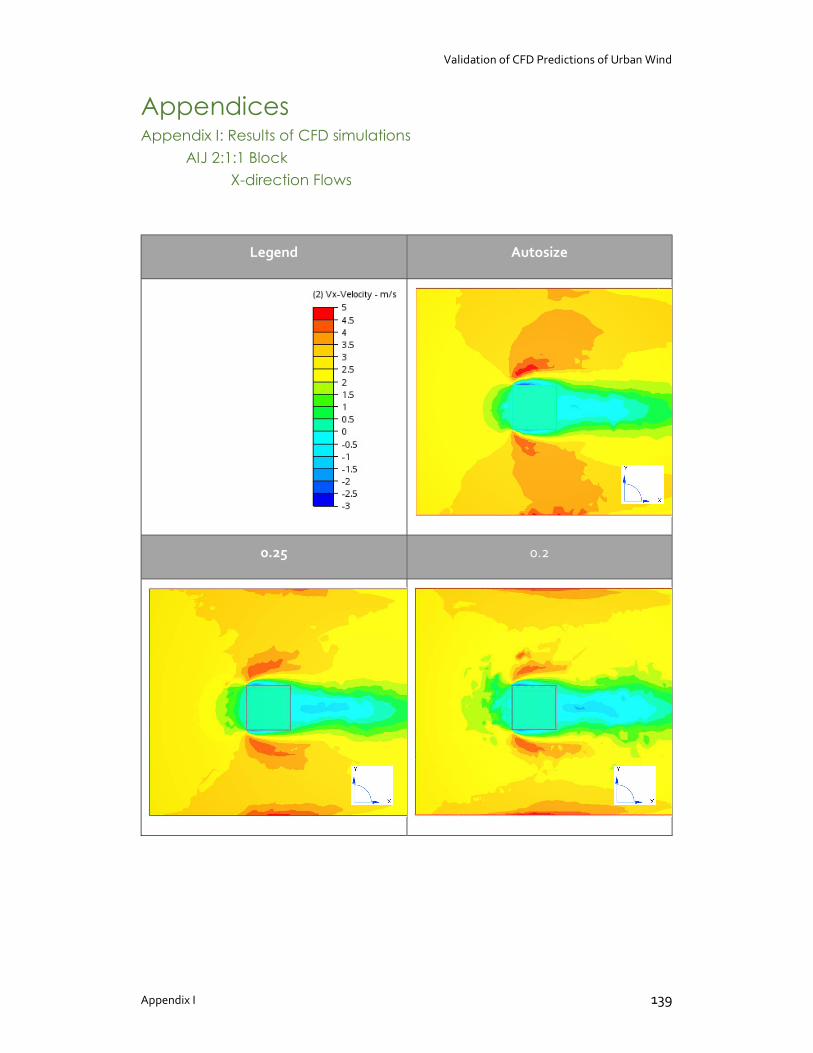
Validation of CFD Predictions of Urban Wind
Appendix I 139
Appendices Appendix I: Results of CFD simulations
AIJ 2:1:1 Block X-direction Flows
Legend Autosize
0.25 0.2
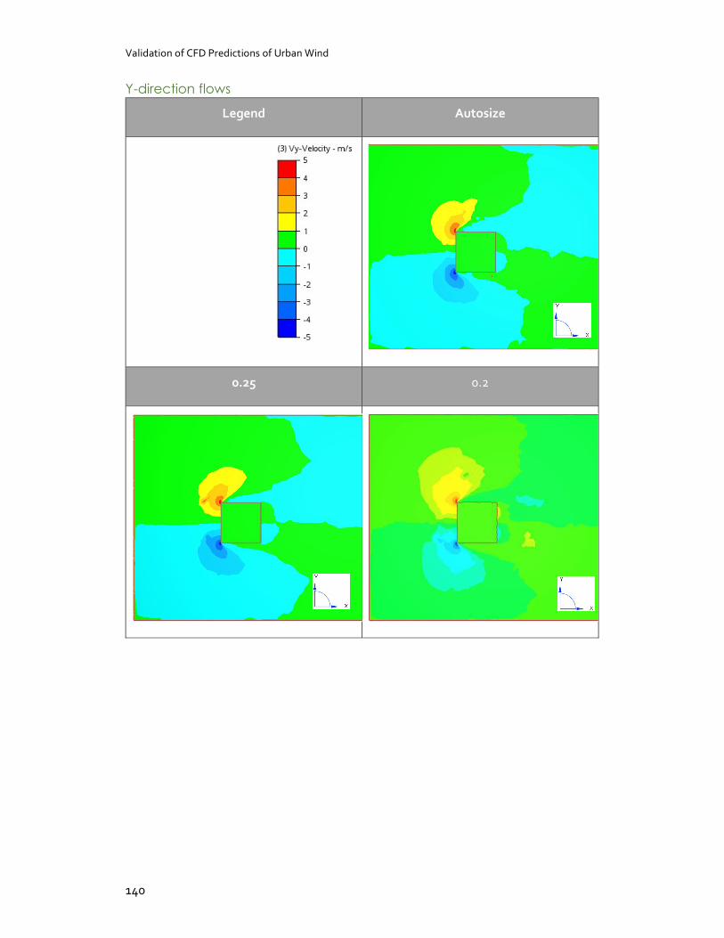
Validation of CFD Predictions of Urban Wind
140
Y-direction flows
Legend Autosize
0.25 0.2
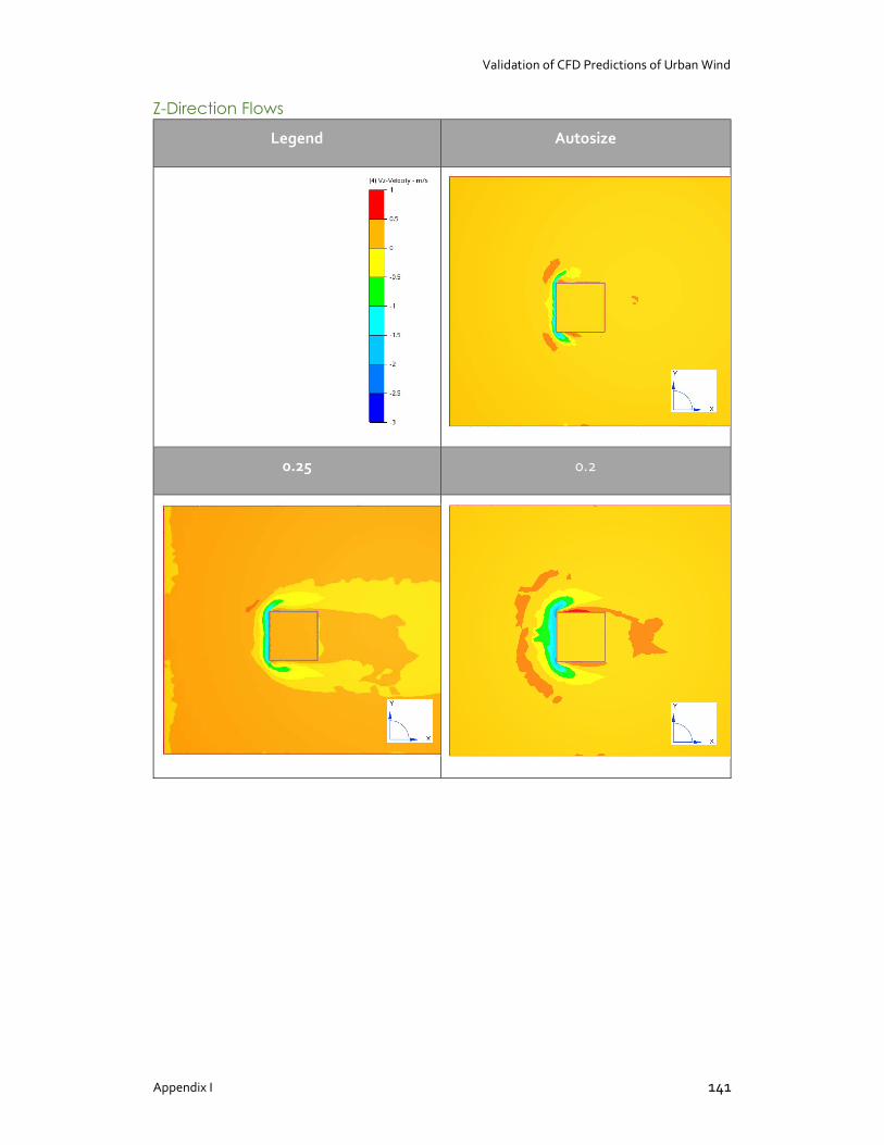
Validation of CFD Predictions of Urban Wind
Appendix I 141
Z-Direction Flows
Legend Autosize
0.25 0.2
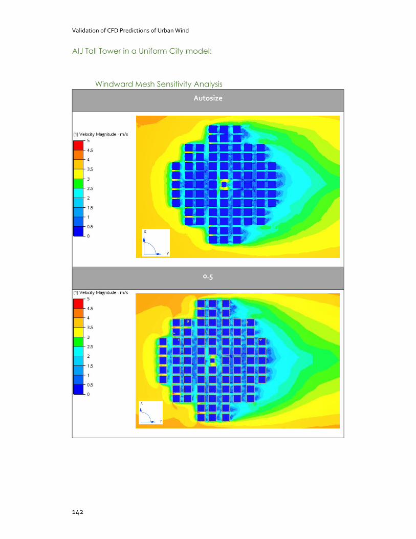
Validation of CFD Predictions of Urban Wind
142
AIJ Tall Tower in a Uniform City model:
Windward Mesh Sensitivity Analysis
Autosize
0.5
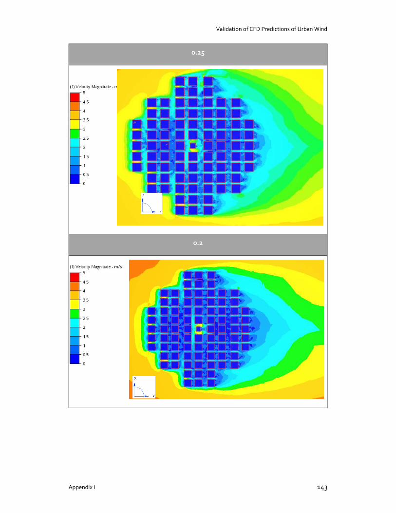
Validation of CFD Predictions of Urban Wind
Appendix I 143
0.25
0.2
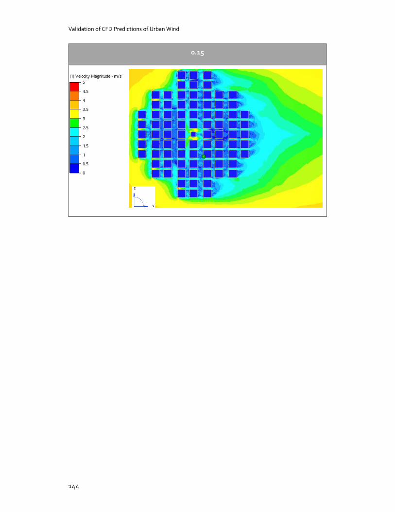
Validation of CFD Predictions of Urban Wind
144
0.15
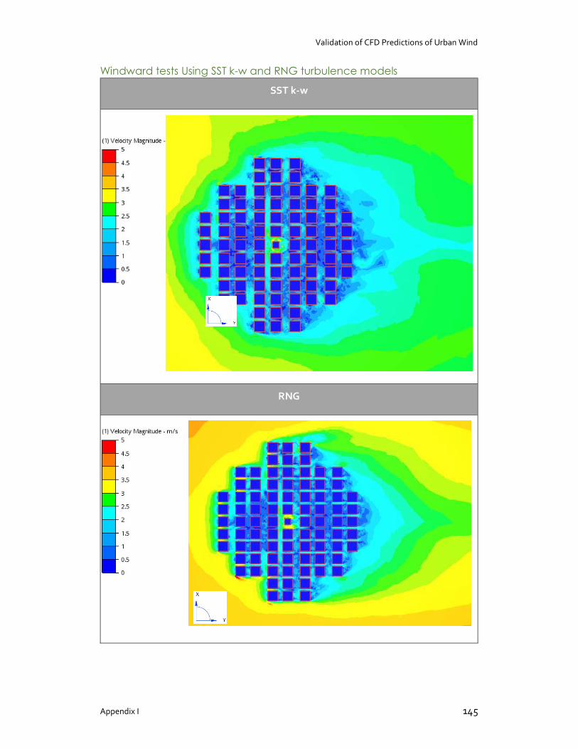
Validation of CFD Predictions of Urban Wind
Appendix I 145
Windward tests Using SST k-w and RNG turbulence models
SST k-w
RNG
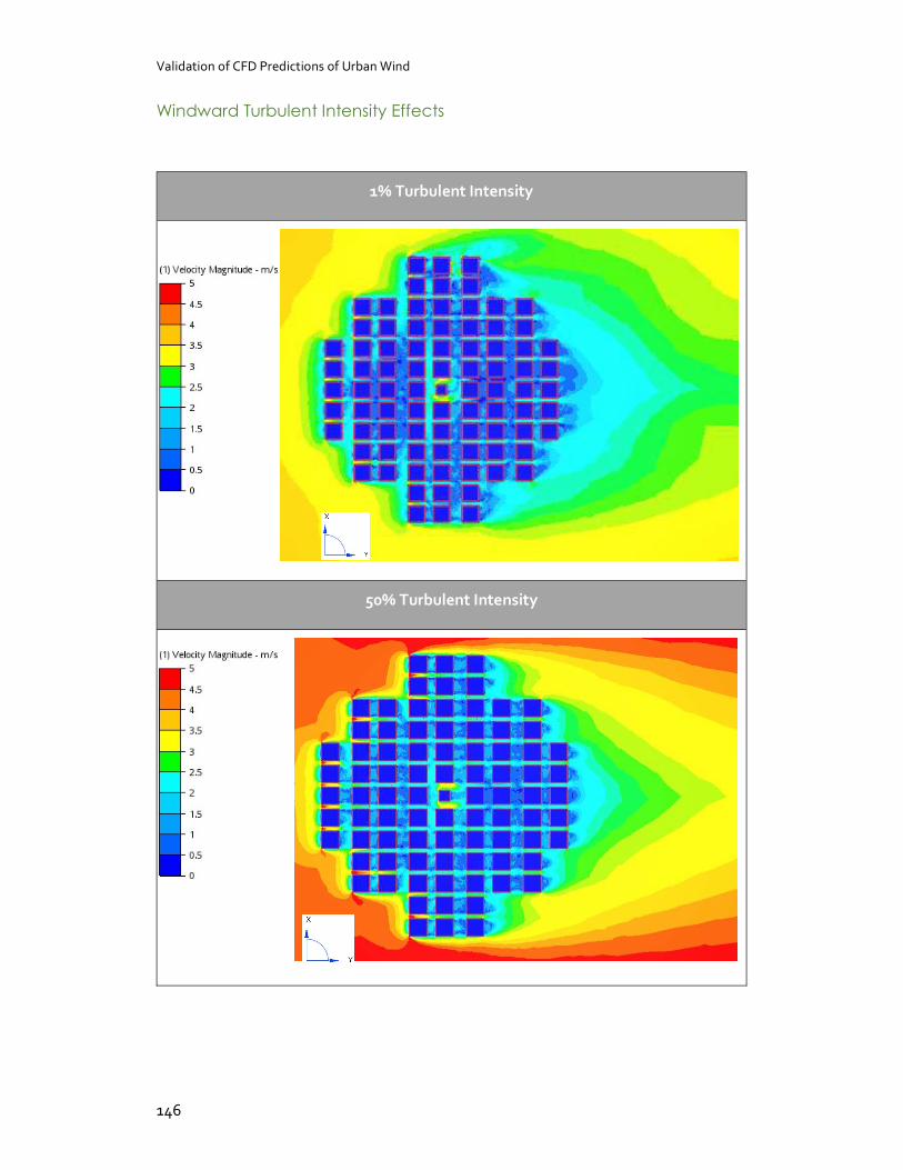
Validation of CFD Predictions of Urban Wind
146
Windward Turbulent Intensity Effects
1% Turbulent Intensity
50% Turbulent Intensity
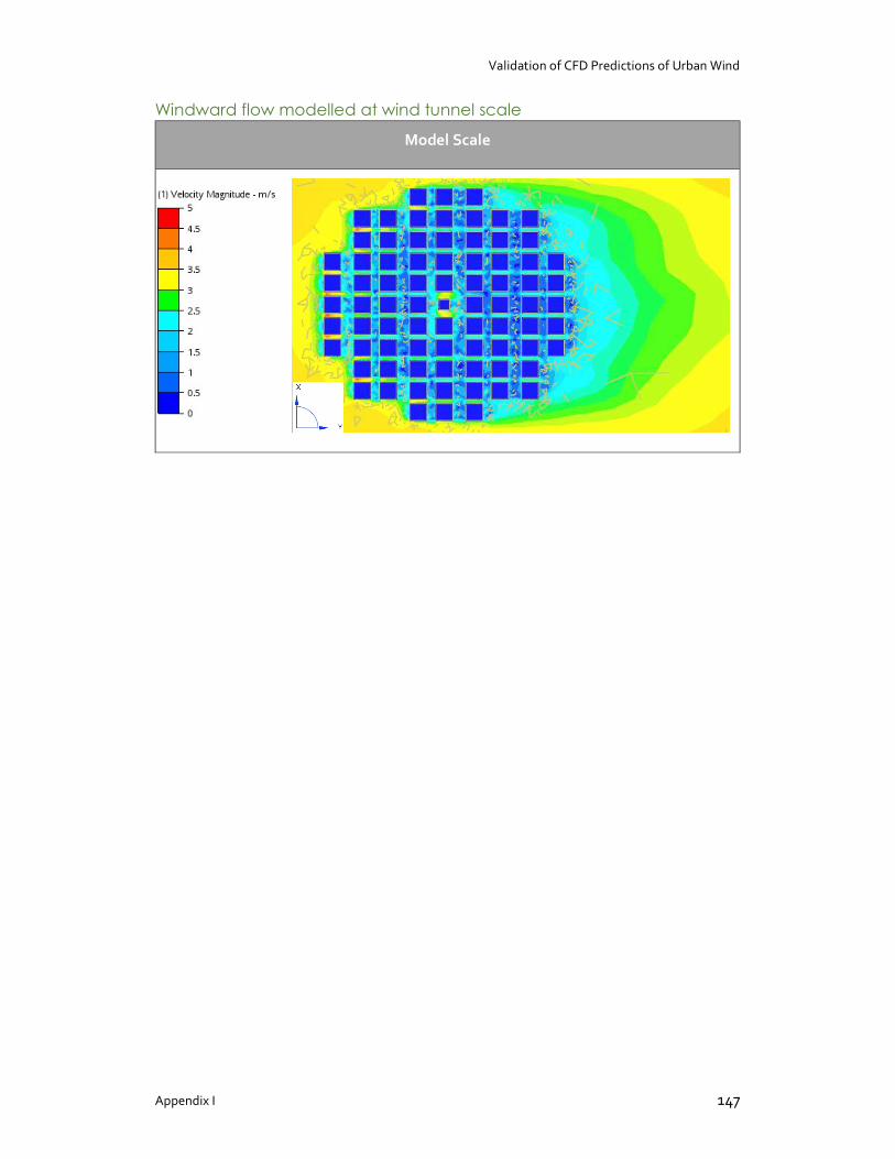
Validation of CFD Predictions of Urban Wind
Appendix I 147
Windward flow modelled at wind tunnel scale
Model Scale
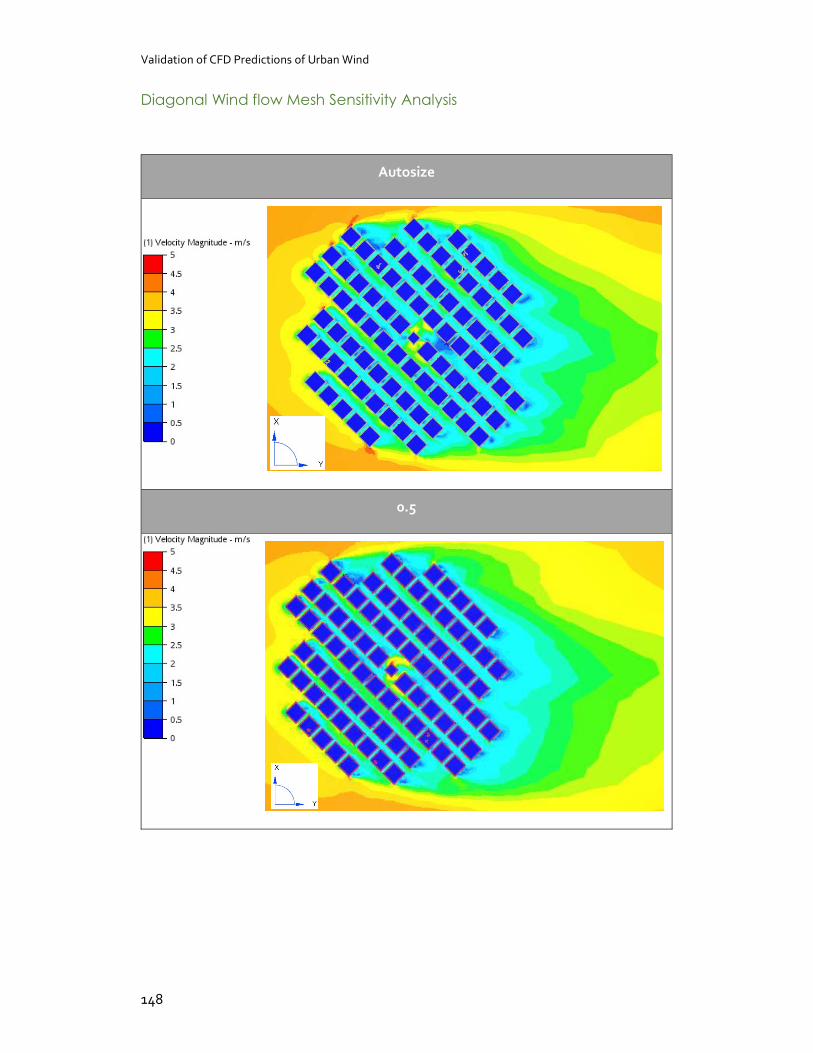
Validation of CFD Predictions of Urban Wind
148
Diagonal Wind flow Mesh Sensitivity Analysis
Autosize
0.5
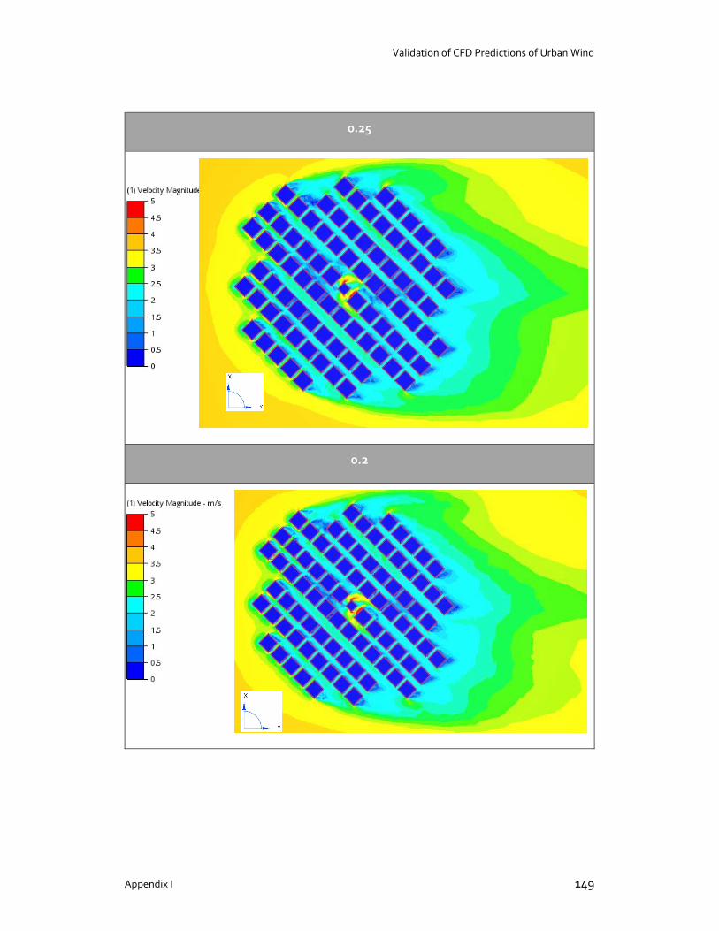
Validation of CFD Predictions of Urban Wind
Appendix I 149
0.25
0.2
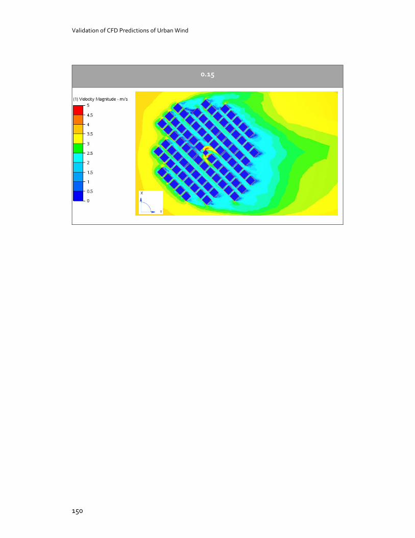
Validation of CFD Predictions of Urban Wind
150
0.15
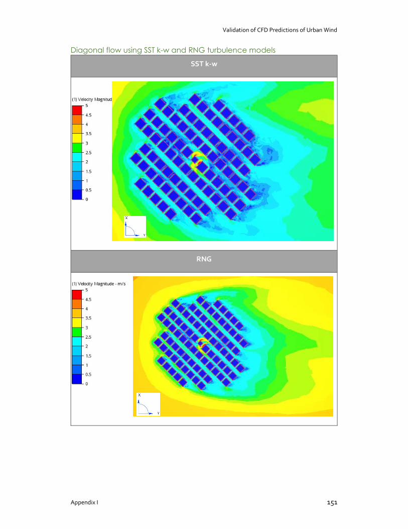
Validation of CFD Predictions of Urban Wind
Appendix I 151
Diagonal flow using SST k-w and RNG turbulence models
SST k-w
RNG
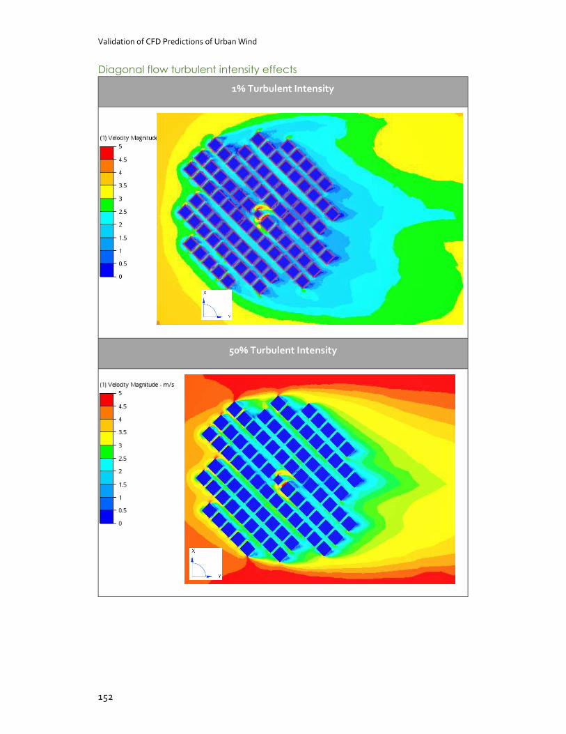
Validation of CFD Predictions of Urban Wind
152
Diagonal flow turbulent intensity effects
1% Turbulent Intensity
50% Turbulent Intensity
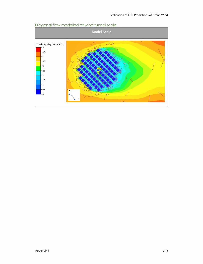
Validation of CFD Predictions of Urban Wind
Appendix I 153
Diagonal flow modelled at wind tunnel scale
Model Scale
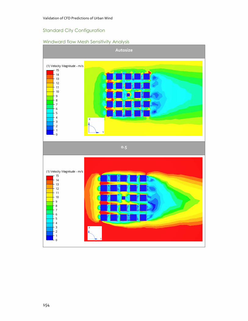
Validation of CFD Predictions of Urban Wind
154
Standard City Configuration
Windward flow Mesh Sensitivity Analysis
Autosize
0.5
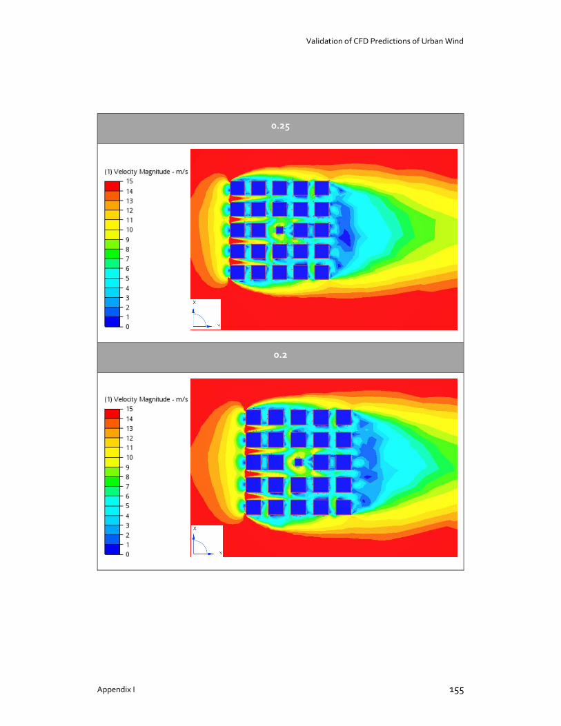
Validation of CFD Predictions of Urban Wind
Appendix I 155
0.25
0.2
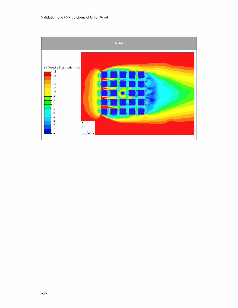
Validation of CFD Predictions of Urban Wind
156
0.15
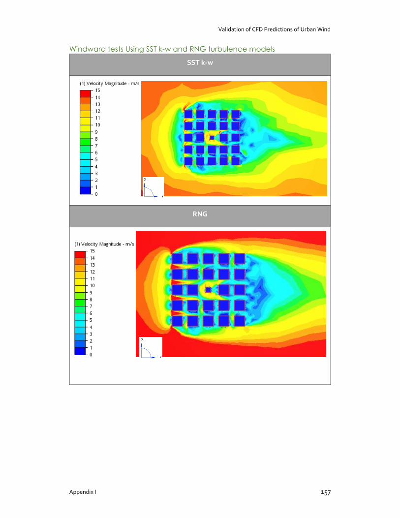
Validation of CFD Predictions of Urban Wind
Appendix I 157
Windward tests Using SST k-w and RNG turbulence models
SST k-w
RNG
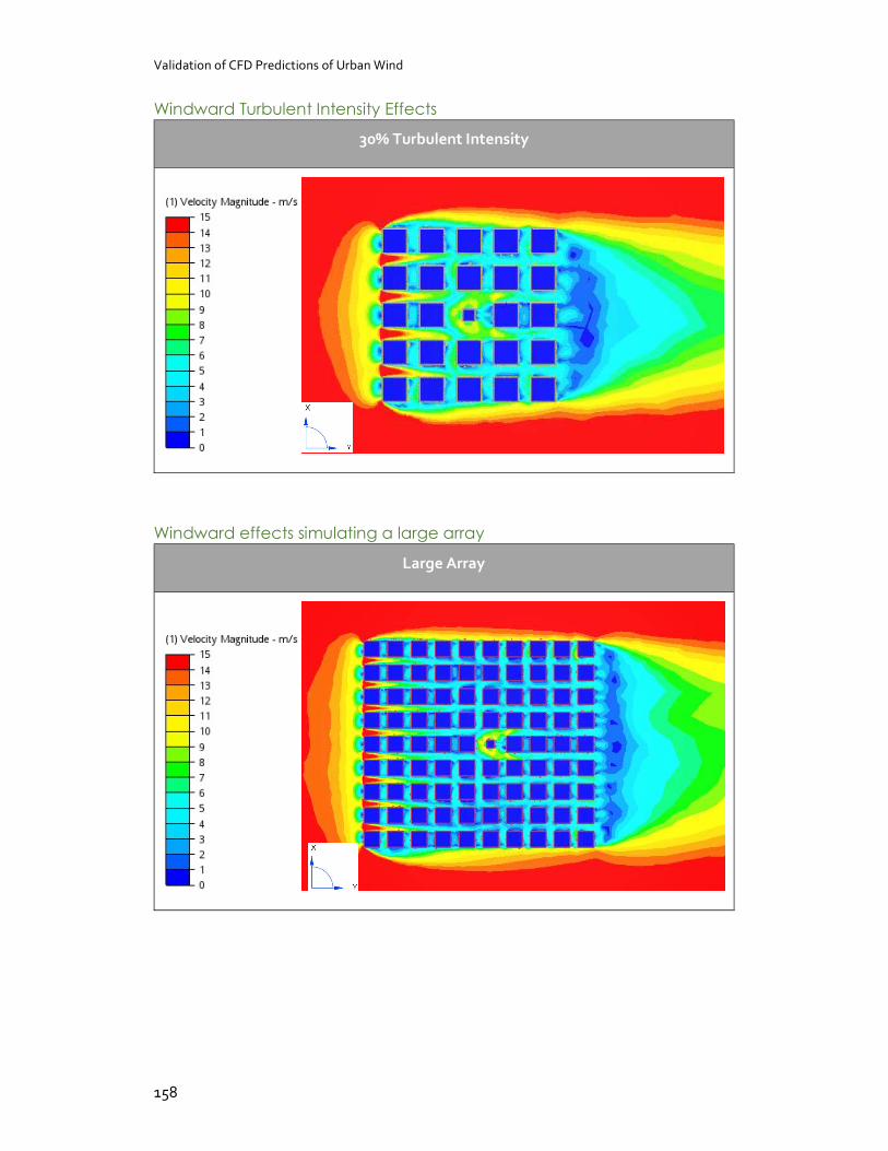
Validation of CFD Predictions of Urban Wind
158
Windward Turbulent Intensity Effects
30% Turbulent Intensity
Windward effects simulating a large array
Large Array
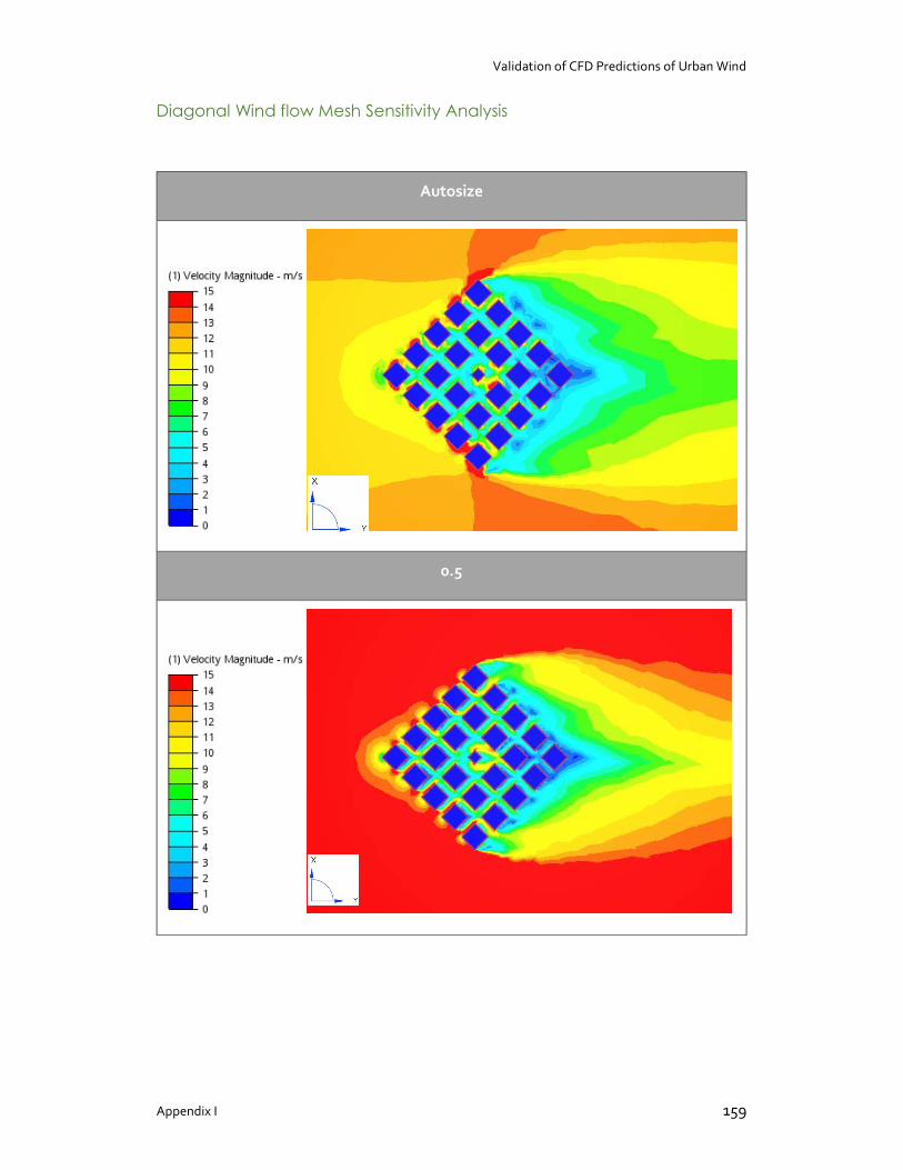
Validation of CFD Predictions of Urban Wind
Appendix I 159
Diagonal Wind flow Mesh Sensitivity Analysis
Autosize
0.5
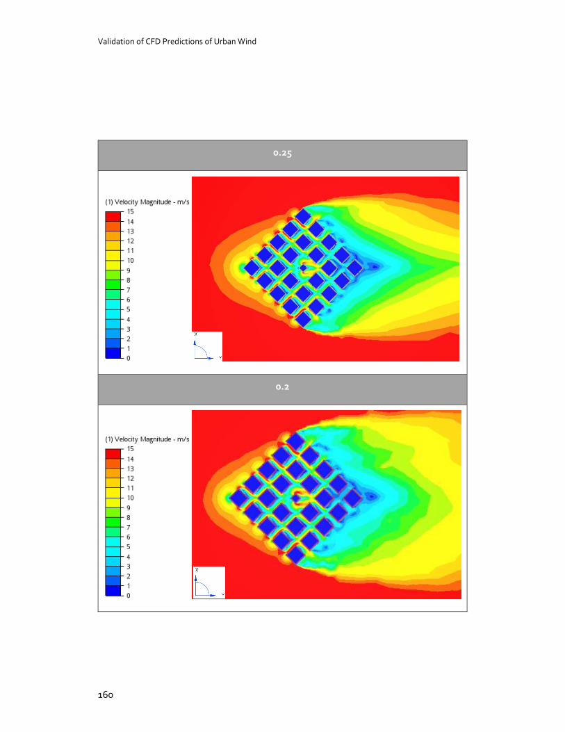
Validation of CFD Predictions of Urban Wind
160
0.25
0.2
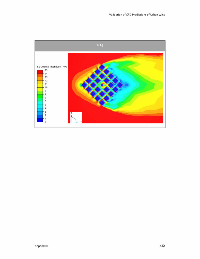
Validation of CFD Predictions of Urban Wind
Appendix I 161
0.15
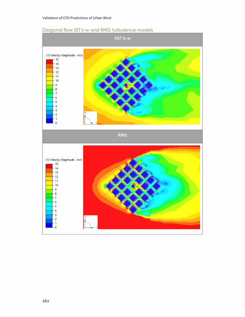
Validation of CFD Predictions of Urban Wind
162
Diagonal flow SST k-w and RNG turbulence models
SST k-w
RNG
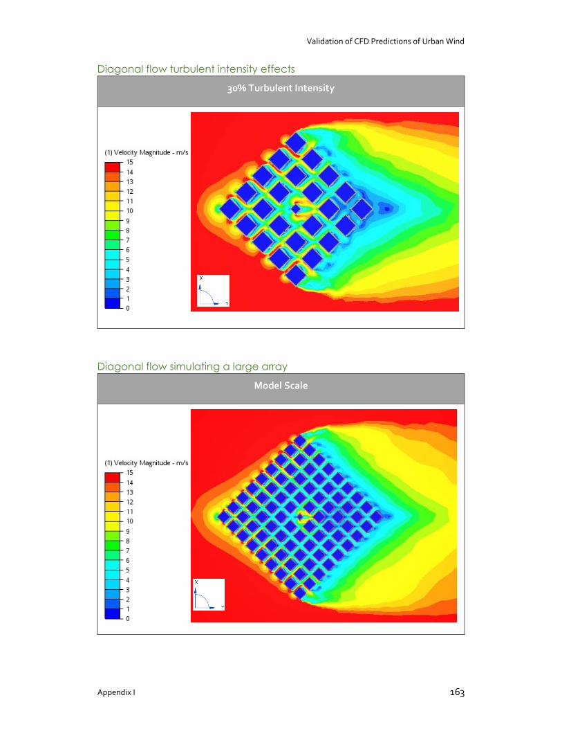
Validation of CFD Predictions of Urban Wind
Appendix I 163
Diagonal flow turbulent intensity effects
30% Turbulent Intensity
Diagonal flow simulating a large array
Model Scale

Validation of CFD Predictions of Urban Wind
164

Validation of CFD Predictions of Urban Wind
Appendix II 165
Appendix II: CFD validation using Lawson Criteria
The Lawson criteria are used for pedestrian wind speed analysis by the City of London corporation (Shilston, 2015). Using the wind speed analysis data generated by the CFD analyses, the same tests carried out in the methodology have been repeated using the Lawson criteria to determine whether the model was sufficiently accurate.
The Lawson Criteria
The Lawson criteria takes the range of mean wind speeds likely to be encountered around a site and divides them up into comfort bands. Each band of wind speeds relates to the maximum allowable force of wind on people undertaking a range of activities, from sitting for long periods to brisk walking.
However, simply assigning a threshold speed does not account for the possibility that this speed may only be reached for a fraction of the time in a year. For this reason, the criteria are a mix of acceptable wind speed thresholds, and acceptable probability of exceedance, in hours per year. For comfort bands in outdoor areas, a threshold of 5% of the hours of the year is set. However, for safety requirements the threshold becomes more stringent, allowing 0.022% of the hours in the year (Shilston, 2015).
For example, if a site was to be designed to fit the Lawson criteria for comfort whilst sitting for long periods, the wind speed must be kept below 4m/s 95% of the hours of the year. However, areas which were not applicable for sitting, such as pedestrian thoroughfares or streets, would not need to meet the requirements for sitting comfort and could allow higher windspeeds.

Validation of CFD Predictions of Urban Wind
166
Table 26: Lawson Criteria, adapted from (Shilston, 2015).
Activity Threshold (m/s)
Can be exceeded (yearly)
Comfort
Sitting for long periods 4 5%
Pedestrian standing / sitting for short periods of time
6 5%
Strolling / leisurely walking 8 5%
“Business walking” 10 5%
Uncomfortable 12 5%
Safety
General public access 15 0.022%
Areas where no “sensitive” people or cyclists will be
20 0.022%
However, the results of wind tunnel tests and CFD analyses are shown as time-averaged measurements. This means that they do not exist as measurements over the course of the year, but rather as a single “snapshot” in time. To be compared against these criteria, they must be converted to a dynamic analysis of the wind speeds which are likely to occur over the course of a year.
To do this regarding Wellington city, the wind tunnel and CFD results were used with historic Wellington meteorological data. The historic data gives the number of hours per year that the wind speed at 150m above Wellington is likely to be equalled or exceeded in any given direction. The wind directions are given in 10° increments, whilst wind speeds are expressed in roughly 1m/s increments up to 32.4m/s.
By multiplying the CFD/wind tunnel ratios by the wind speeds at 150m, the number of hours that the pedestrian level wind speeds exceed the Lawson Criteria could be

Validation of CFD Predictions of Urban Wind
Appendix II 167
ascertained. However, wind direction also plays an important role. The Wellington city wind data sheets cover 36 10° increments, but the configurations provided wind measurements for 2 directions: 0° and 45°. This was an issue, as the historic wellington wind data does not provide data for 45° winds. Also, all 8760 hours of the year, which the Lawson Criteria are based on, cannot be accounted for unless each wind direction is included in the calculation.
To solve this issue, the 10° increments were combined to represent wind coming from 4 directions: northerly, southerly, easterly and westerly. This is not dissimilar to the wind tunnel test practice for new buildings, which tests for 8 wind directions. By combining the incremental directions, the total hours for each wind direction were aggregated, which allowed all the hours in the year to be considered. Because the configurations are identical, having the measurements for 2 directions is effectively the same as having measurements for 4 directions, as the results would not change with the wind coming from the opposite direction.
The same method was applied to the AIJ dataset, however the wind tunnel and CFD results for this set were normalised by the wind speeds at 100m, rather than 150m. Because the wind profile used by the AIJ dataset followed the same power law curve as the Standard City set, the Wellington wind data could be interpolated to fit the AIJ curve. This was achieved using the power law described by Gandemer (1975):
=
Where:
= Mean wind speed at site (m/s) = Mean wind speed at boundary layer
= Measurement height at site (m) = Height of boundary layer
= terrain roughness coefficient (0.35 for city terrain)
Normalising the Standard City data allows the same type of validation analysis to be carried out on both configurations.
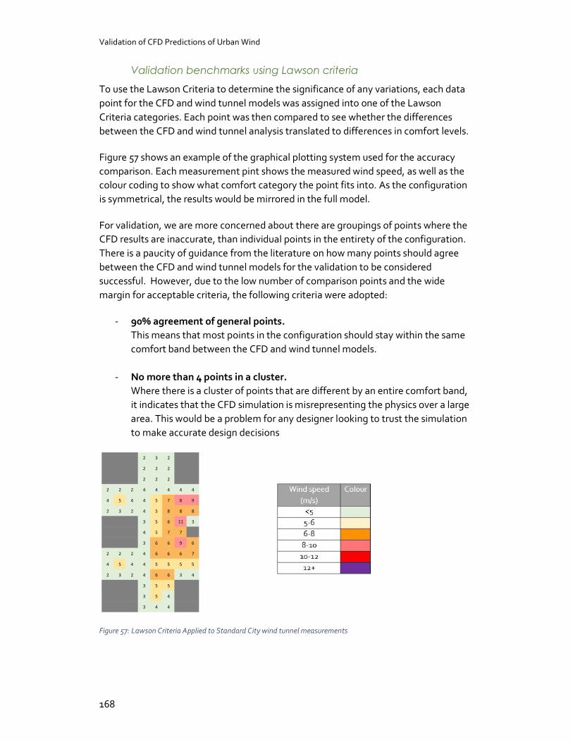
Validation of CFD Predictions of Urban Wind
168
Validation benchmarks using Lawson criteria
To use the Lawson Criteria to determine the significance of any variations, each data point for the CFD and wind tunnel models was assigned into one of the Lawson Criteria categories. Each point was then compared to see whether the differences between the CFD and wind tunnel analysis translated to differences in comfort levels.
Figure 57 shows an example of the graphical plotting system used for the accuracy comparison. Each measurement pint shows the measured wind speed, as well as the colour coding to show what comfort category the point fits into. As the configuration is symmetrical, the results would be mirrored in the full model.
For validation, we are more concerned about there are groupings of points where the CFD results are inaccurate, than individual points in the entirety of the configuration. There is a paucity of guidance from the literature on how many points should agree between the CFD and wind tunnel models for the validation to be considered successful. However, due to the low number of comparison points and the wide margin for acceptable criteria, the following criteria were adopted:
- 90% agreement of general points. This means that most points in the configuration should stay within the same comfort band between the CFD and wind tunnel models.
- No more than 4 points in a cluster. Where there is a cluster of points that are different by an entire comfort band, it indicates that the CFD simulation is misrepresenting the physics over a large area. This would be a problem for any designer looking to trust the simulation to make accurate design decisions
Figure 57: Lawson Criteria Applied to Standard City wind tunnel measurements
2 3 2
2 2 2
2 2 2
2 2 2 4 4 4 4 4
4 5 4 4 5 7 8 9
2 3 2 4 5 8 8 8
3 5 6 11 3
4 5 7 7
3 6 6 9 6
2 2 2 4 6 6 6 7
4 5 4 4 5 5 5 5
2 3 2 4 6 6 3 4
3 5 5
3 5 4
3 4 4
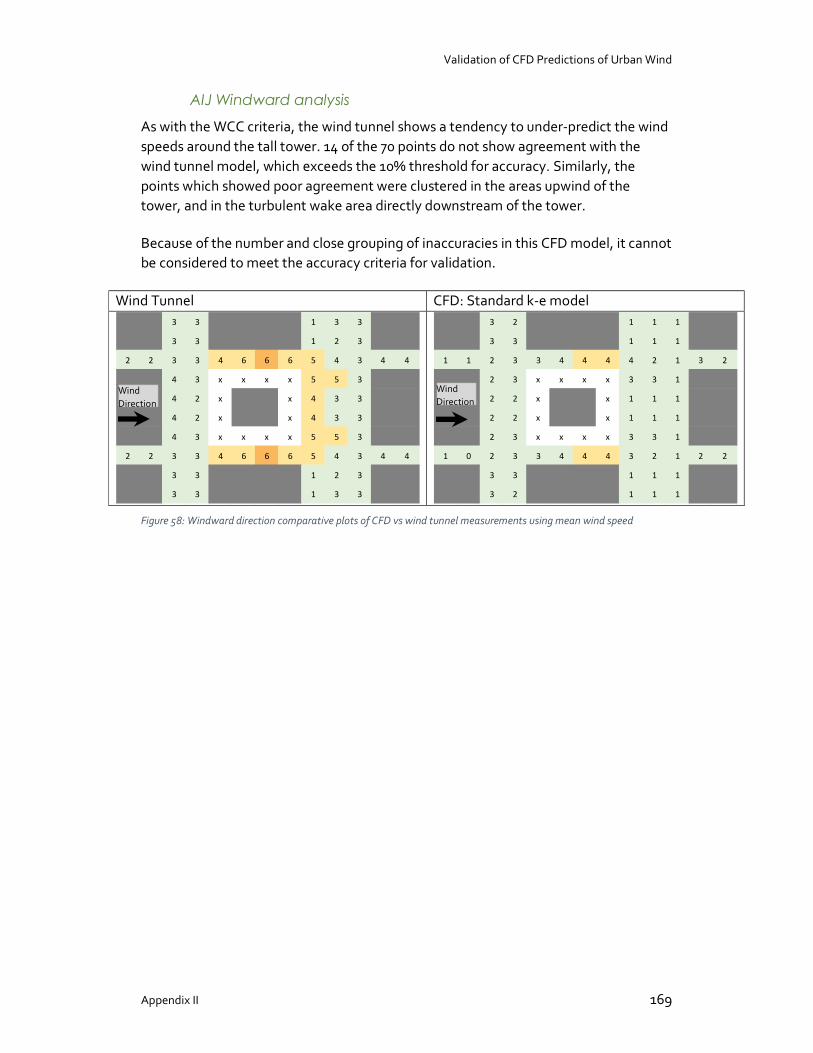
Validation of CFD Predictions of Urban Wind
Appendix II 169
AIJ Windward analysis
As with the WCC criteria, the wind tunnel shows a tendency to under-predict the wind speeds around the tall tower. 14 of the 70 points do not show agreement with the wind tunnel model, which exceeds the 10% threshold for accuracy. Similarly, the points which showed poor agreement were clustered in the areas upwind of the tower, and in the turbulent wake area directly downstream of the tower.
Because of the number and close grouping of inaccuracies in this CFD model, it cannot be considered to meet the accuracy criteria for validation.
Wind Tunnel CFD: Standard k-e model
Figure 58: Windward direction comparative plots of CFD vs wind tunnel measurements using mean wind speed
3 3 1 3 3
3 3 1 2 3
2 2 3 3 4 6 6 6 5 4 3 4 4
4 3 x x x x 5 5 3
4 2 x x 4 3 3
4 2 x x 4 3 3
4 3 x x x x 5 5 3
2 2 3 3 4 6 6 6 5 4 3 4 4
3 3 1 2 3
3 3 1 3 3
3 2 1 1 1
3 3 1 1 1
1 1 2 3 3 4 4 4 4 2 1 3 2
2 3 x x x x 3 3 1
2 2 x x 1 1 1
2 2 x x 1 1 1
2 3 x x x x 3 3 1
1 0 2 3 3 4 4 4 3 2 1 2 2
3 3 1 1 1
3 2 1 1 1
Wind Direction
Wind Direction
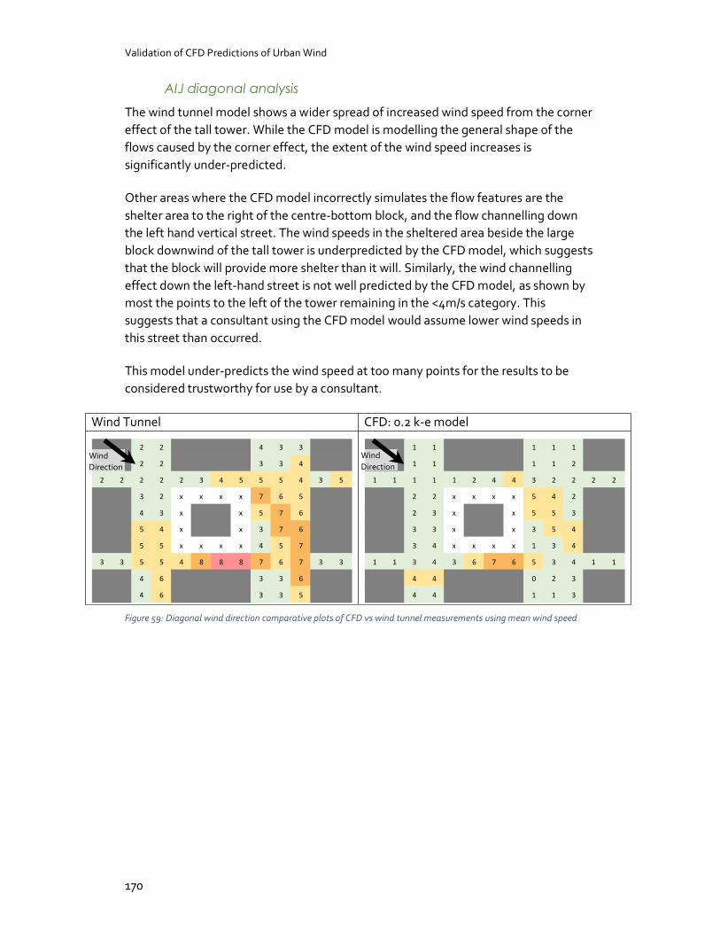
Validation of CFD Predictions of Urban Wind
170
AIJ diagonal analysis
The wind tunnel model shows a wider spread of increased wind speed from the corner effect of the tall tower. While the CFD model is modelling the general shape of the flows caused by the corner effect, the extent of the wind speed increases is significantly under-predicted.
Other areas where the CFD model incorrectly simulates the flow features are the shelter area to the right of the centre-bottom block, and the flow channelling down the left hand vertical street. The wind speeds in the sheltered area beside the large block downwind of the tall tower is underpredicted by the CFD model, which suggests that the block will provide more shelter than it will. Similarly, the wind channelling effect down the left-hand street is not well predicted by the CFD model, as shown by most the points to the left of the tower remaining in the <4m/s category. This suggests that a consultant using the CFD model would assume lower wind speeds in this street than occurred.
This model under-predicts the wind speed at too many points for the results to be considered trustworthy for use by a consultant.
Wind Tunnel CFD: 0.2 k-e model
Figure 59: Diagonal wind direction comparative plots of CFD vs wind tunnel measurements using mean wind speed
2 2 4 3 3
2 2 3 3 4
2 2 2 2 2 3 4 5 5 5 4 3 5
3 2 x x x x 7 6 5
4 3 x x 5 7 6
5 4 x x 3 7 6
5 5 x x x x 4 5 7
3 3 5 5 4 8 8 8 7 6 7 3 3
4 6 3 3 6
4 6 3 3 5
1 1 1 1 1
1 1 1 1 2
1 1 1 1 1 2 4 4 3 2 2 2 2
2 2 x x x x 5 4 2
2 3 x x 5 5 3
3 3 x x 3 5 4
3 4 x x x x 1 3 4
1 1 3 4 3 6 7 6 5 3 4 1 1
4 4 0 2 3
4 4 1 1 3
Wind Direction
Wind Direction
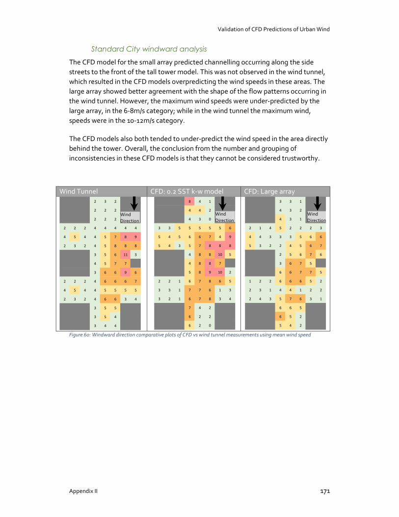
Validation of CFD Predictions of Urban Wind
Appendix II 171
Standard City windward analysis
The CFD model for the small array predicted channelling occurring along the side streets to the front of the tall tower model. This was not observed in the wind tunnel, which resulted in the CFD models overpredicting the wind speeds in these areas. The large array showed better agreement with the shape of the flow patterns occurring in the wind tunnel. However, the maximum wind speeds were under-predicted by the large array, in the 6-8m/s category; while in the wind tunnel the maximum wind, speeds were in the 10-12m/s category.
The CFD models also both tended to under-predict the wind speed in the area directly behind the tower. Overall, the conclusion from the number and grouping of inconsistencies in these CFD models is that they cannot be considered trustworthy.
Wind Tunnel CFD: 0.2 SST k-w model CFD: Large array
Figure 60: Windward direction comparative plots of CFD vs wind tunnel measurements using mean wind speed
2 3 2
2 2 2
2 2 2
2 2 2 4 4 4 4 4
4 5 4 4 5 7 8 9
2 3 2 4 5 8 8 8
3 5 6 11 3
4 5 7 7
3 6 6 9 6
2 2 2 4 6 6 6 7
4 5 4 4 5 5 5 5
2 3 2 4 6 6 3 4
3 5 5
3 5 4
3 4 4
8 4 1
4 4 2
4 3 0
3 3 5 5 5 5 5 6
5 4 5 6 6 7 4 9
5 4 3 5 7 8 8 8
4 8 8 10 5
4 8 8 7
5 8 9 10 2
2 2 1 6 7 8 6 5
3 3 1 7 7 6 1 3
3 2 1 6 7 8 3 4
7 4 2
6 2 2
6 2 0
3 3 1
4 3 2
4 3 1
2 1 4 5 2 2 2 3
4 4 3 3 3 5 6 6
5 3 2 2 4 5 6 7
2 5 6 7 6
3 6 7 5
6 6 7 7 5
1 2 2 6 6 6 5 2
2 3 1 4 4 1 2 2
2 4 3 5 7 6 3 1
6 6 5
6 5 2
5 4 2
Wind Direction
Wind Direction
Wind Direction
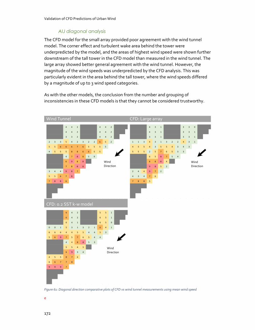
Validation of CFD Predictions of Urban Wind
172
AIJ diagonal analysis
The CFD model for the small array provided poor agreement with the wind tunnel model. The corner effect and turbulent wake area behind the tower were underpredicted by the model, and the areas of highest wind speed were shown further downstream of the tall tower in the CFD model than measured in the wind tunnel. The large array showed better general agreement with the wind tunnel. However, the magnitude of the wind speeds was underpredicted by the CFD analysis. This was particularly evident in the area behind the tall tower, where the wind speeds differed by a magnitude of up to 3 wind speed categories.
As with the other models, the conclusion from the number and grouping of inconsistencies in these CFD models is that they cannot be considered trustworthy.
Wind Tunnel CFD: Large array
CFD: 0.2 SST k-w model
Figure 61: Diagonal direction comparative plots of CFD vs wind tunnel measurements using mean wind speed
e
4 4 2 4 4 2
4 4 2 4 4 2
3 3 2 4 4 2
2 3 3 5 4 2 3 2 2 6 5 2
5 5 6 6 6 7 6 5 5 5 5
4 5 5 5 8 8 6 6 5 5
4 7 8 8 5 9
6 9 8 8
7 8 8 8
3 4 4 9 8 7
5 5 6 7 8
7 8 8 6
4 3 1 3 3 0
4 3 1 3 3 1
3 3 1 3 3 1
1 1 3 4 3 1 3 2 2 4 3 1
4 5 5 4 3 5 5 4 3 4 3
5 5 5 2 5 7 6 5 3 3
6 5 8 7 5 4
8 8 8 4
9 8 5 2
2 4 4 9 7 2
4 3 4 7 6
7 8 8 5
6 4 2 5 5 1
6 4 2 6 5 1
6 4 1 6 5 0
0 0 1 5 3 1 3 2 1 6 4 1
6 6 6 4 4 5 5 4 4 5 3
5 6 9 7 5 7 6 5 4 4
4 4 8 8 5 3
5 5 4 5
6 9 3 4
4 5 5 8 7 4
6 6 7 7 8
9 9 9 7
Wind Direction
Wind Direction
Wind Direction