risks

Article

Valuation of Large Variable Annuity Portfolios UsingLinear Models with Interactions

Guojun Gan ID

Department of Mathematics, University of Connecticut, Storrs, CT 06269-1009, USA; guojun.gan@uconn.edu;Tel.: +1-860-486-3919

Received: 28 June 2018; Accepted: 12 July 2018; Published: 12 July 2018�����������������

Abstract: A variable annuity is a popular life insurance product that comes with financial guarantees.Using Monte Carlo simulation to value a large variable annuity portfolio is extremely time-consuming.Metamodeling approaches have been proposed in the literature to speed up the valuation process.In metamodeling, a metamodel is first fitted to a small number of variable annuity contracts and thenused to predict the values of all other contracts. However, metamodels that have been investigatedin the literature are sophisticated predictive models. In this paper, we investigate the use of linearregression models with interaction effects for the valuation of large variable annuity portfolios.Our numerical results show that linear regression models with interactions are able to produceaccurate predictions and can be useful additions to the toolbox of metamodels that insurancecompanies can use to speed up the valuation of large VA portfolios.

Keywords: variable annuity; portfolio valuation; linear regression; group-lasso; interaction effect

1. Introduction

A variable annuity (VA) is a life insurance product created by insurance companies to addressconcerns that many people have about outliving their assets (Ledlie et al. 2008; The Geneva AssociationReport 2013). Under a VA contract, the policyholder makes one lump-sum or a series of purchasepayments to the insurance company and in turn, the insurance company makes benefit paymentsto the policyholder beginning immediately or at some future date. A typical VA has two phases:the accumulation phase and the payout phase. During the accumulation phase, the policyholderbuilds assets for retirement by investing the money in some investment funds provided by the insurer.During the payout phase, the policyholder receives benefit payments in either a lump-sum, periodicwithdrawals or an ongoing income stream. The amount of benefit payments is tied to the performanceof the investment portfolio selected by the policyholder.

To protect the policyholder’s capital against market downturns, VAs are designed to includevarious guarantees that share some similarities with the standard options traded in exchanges(Hardy 2003). These guarantees can be divided into two broad categories: death benefits and livingbenefits. A guaranteed minimum death benefit (GMDB) guarantees a specified lump sum to thebeneficiary upon the death of the policyholder regardless of the performance of the investment portfolio.There are several types of living benefits. Popular living benefits include the guaranteed minimumwithdrawal benefit (GMWB), the guaranteed minimum income benefit (GMIB), the guaranteedminimum maturity benefit (GMMB), and the guaranteed minimum accumulation benefit (GMAB).A GMWB guarantees that the policyholder can make systematic annual withdrawals of a specifiedamount from the benefit base over a period of time, even though the investment portfolio might bedepleted. A GMIB guarantees that the policyholder can convert the greater of the actual account valueor the benefit base to an annuity according to a specified rate. A GMMB guarantees the policyholder aspecific amount at the maturity of the contract. A GMAB guarantees that the policyholder can renew

Risks 2018, 6, 71; doi:10.3390/risks6030071 www.mdpi.com/journal/risks

Risks 2018, 6, 71 2 of 19

the contract during a specified window after a specified waiting period, which is usually 10 years(Brown et al. 2002).

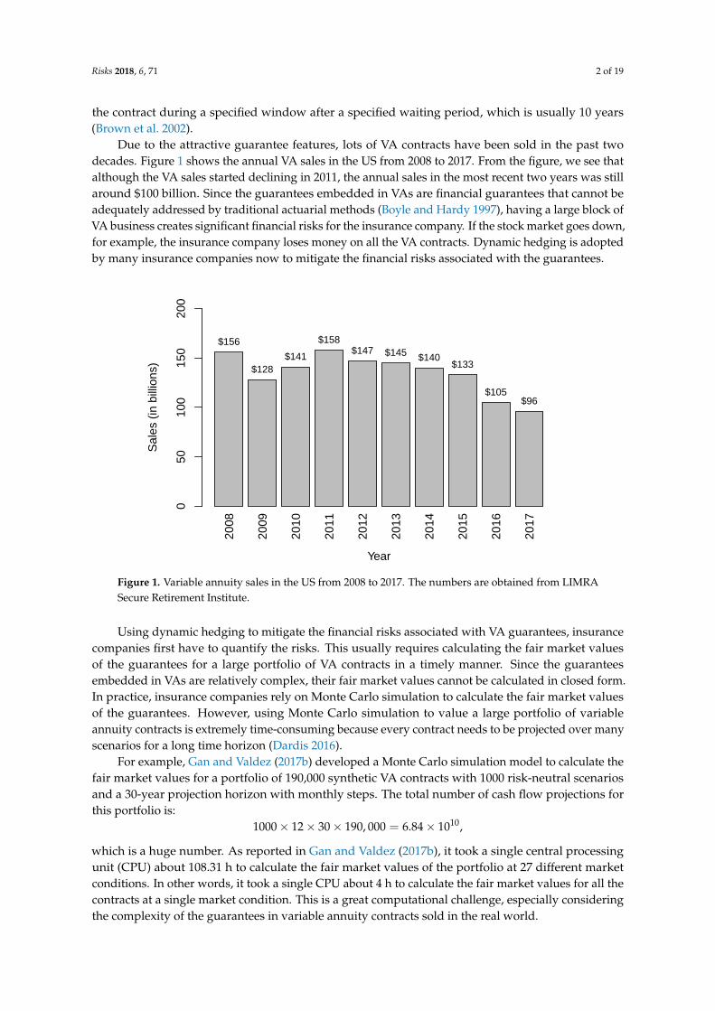
Due to the attractive guarantee features, lots of VA contracts have been sold in the past twodecades. Figure 1 shows the annual VA sales in the US from 2008 to 2017. From the figure, we see thatalthough the VA sales started declining in 2011, the annual sales in the most recent two years was stillaround $100 billion. Since the guarantees embedded in VAs are financial guarantees that cannot beadequately addressed by traditional actuarial methods (Boyle and Hardy 1997), having a large block ofVA business creates significant financial risks for the insurance company. If the stock market goes down,for example, the insurance company loses money on all the VA contracts. Dynamic hedging is adoptedby many insurance companies now to mitigate the financial risks associated with the guarantees.

Year

Sal

es (

in b

illio

ns)

050

100

150

200

$156

$128$141

$158$147 $145 $140

$133

$105$96

2008

2009

2010

2011

2012

2013

2014

2015

2016

2017

Figure 1. Variable annuity sales in the US from 2008 to 2017. The numbers are obtained from LIMRASecure Retirement Institute.

Using dynamic hedging to mitigate the financial risks associated with VA guarantees, insurancecompanies first have to quantify the risks. This usually requires calculating the fair market valuesof the guarantees for a large portfolio of VA contracts in a timely manner. Since the guaranteesembedded in VAs are relatively complex, their fair market values cannot be calculated in closed form.In practice, insurance companies rely on Monte Carlo simulation to calculate the fair market valuesof the guarantees. However, using Monte Carlo simulation to value a large portfolio of variableannuity contracts is extremely time-consuming because every contract needs to be projected over manyscenarios for a long time horizon (Dardis 2016).

For example, Gan and Valdez (2017b) developed a Monte Carlo simulation model to calculate thefair market values for a portfolio of 190,000 synthetic VA contracts with 1000 risk-neutral scenariosand a 30-year projection horizon with monthly steps. The total number of cash flow projections forthis portfolio is:

1000× 12× 30× 190, 000 = 6.84× 1010,

which is a huge number. As reported in Gan and Valdez (2017b), it took a single central processingunit (CPU) about 108.31 h to calculate the fair market values of the portfolio at 27 different marketconditions. In other words, it took a single CPU about 4 h to calculate the fair market values for all thecontracts at a single market condition. This is a great computational challenge, especially consideringthe complexity of the guarantees in variable annuity contracts sold in the real world.

Risks 2018, 6, 71 3 of 19

Recently, metamodeling approaches have been proposed to address the aforementionedcomputational problem. See, for example, Gan (2013); Gan and Lin (2015); Gan (2015); Hejazi andJackson (2016); Gan and Valdez (2016); Gan and Valdez (2017a); Gan and Lin (2017); Hejazi et al. (2017);Gan and Huang (2017); Xu et al. (2018); and Gan and Valdez (2018). In metamodeling, a metamodel,which is a model of the Monte Carlo simulation model, is built to replace the Monte Carlo simulationmodel to value the VA contracts in a large portfolio. Using metamodeling approaches can reducesignificantly the runtime of valuing a large portfolio of VA contracts for the following reasons:

• Building a metamodel only requires using the Monte Carlo simulation model to value a smallnumber of representative VA contracts.

• The metamodel is usually much simpler and faster than the Monte Carlo simulation model.

The metamodels (e.g., kriging, GB2 regression, and neural networks mentioned in Section 3)investigated in the aforementioned papers are sophisticated predictive models, which might causedifficulties in terms of interpretation or calibration. For example, fitting the GB2 regression model tothe data is quite challenging (Gan and Valdez 2018). In this paper, we explore the use of linear modelswith interaction effects for the valuation of large VA portfolios. Unlike these existing metamodels,lines models have the advantages that they are well-known, can be fitted to data easily, and can beinterpreted straightforwardly. Including the interaction effects between the features (e.g., gender,product type, account values) of VA contracts can improve the performance of linear models.

This paper is structured as follows. In Section 2, we give a description of the data we use todemonstrate the usefulness of modeling interactions for VA valuation. In Section 3, we provide areview of existing metamodeling approaches. In Section 4, we introduce the group-lasso and theoverlapped group-lasso briefly. In Section 5, we present some numerical results. Finally, Section 6concludes the paper with some remarks.

2. Description of the Data

To demonstrate the benefit of including interactions in regression models, we use a syntheticdataset obtained from Gan and Valdez (2017b). This dataset contains 190,000 VA policies, each ofwhich is described by 45 features or variables. Since some of the variables have identical values,we exclude these variables from the regression analysis. The explanatory variables used to buildregression models are described in Table 1. Among these variables, gender and productType are theonly categorical variables.

Table 1. Variables of VA contracts.

Variable Description

gender Gender of the policyholderproductType Product type of the VA contract

gmwbBalance GMWB balancegbAmt Guaranteed benefit amount

FundValuei Account value of the ith fund, for i = 1, 2, . . . , 10age Age of the policyholderttm Time to maturity in years

There are 19 types of VA contracts in the dataset. There are an equal number of VA contractsin each type, that is, there are 10,000 VA contracts of each type. For each type of VA contract, about40% of the policyholders are female. Overall, 76,007 VA contractholders are female and 113,993 aremale. Table 2 shows some summary statistics of the continuous explanatory variables and the responsevariable, which is the fair market value. From the table, we see that most of the contracts have zerogmwbBalance because most of the contracts do not include a GMWB. For every investment fund,many contracts have zero account values because many policyholders did not invest in the fund.The maturity of the contracts ranges from less than 1 year to about 29 years.

Risks 2018, 6, 71 4 of 19

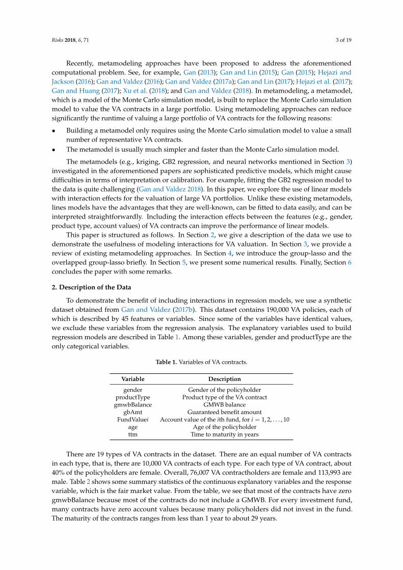
Table 2 also shows the summary statistics of the fair market value, which is the response variable.The fair market value is calculated as the difference between the benefit and the risk charge. When thebenefit is less than the risk charge, the fair market value is negative; otherwise, the fair market value ispositive. Figure 2 shows a histogram of the fair market values. From the figure, we see that most of thefair market values are positive and the distribution is positively skewed. Regarding the runtime usedby the Monte Carlo simulation to calculate these fair market values, it was about 108 h if a single CPUwas used. See Gan and Valdez (2017b) for details.

Table 2. Summary statistics of the continuous explanatory variables and the response variable.

Variable Min 1st Q Median 3rd Q Max

gmwbBalance 0.00 0.00 0.00 0.00 499,708.73gbAmt 0.00 186,864.95 316,225.98 445,940.63 1,105,731.57

FundValue1 0.00 0.00 12,635.17 49,764.15 1,099,204.71FundValue2 0.00 0.00 15,107.17 56,882.55 1,136,895.87FundValue3 0.00 0.00 10,043.96 39,199.69 752,945.34FundValue4 0.00 0.00 10,383.79 39,519.79 610,579.68FundValue5 0.00 0.00 9221.26 35,023.00 498,479.36FundValue6 0.00 0.00 13,881.41 52,981.06 1,091,155.87FundValue7 0.00 0.00 11,541.47 44,465.70 834,253.63FundValue8 0.00 0.00 11,931.41 45,681.16 725,744.64FundValue9 0.00 0.00 11,562.79 44,302.35 927,513.49

FundValue10 0.00 0.00 11,850.05 44,967.78 785,978.60age 34.52 42.03 49.45 56.96 64.46ttm 0.59 10.34 14.51 18.76 28.52fmv −94,944.17 −5142.94 12,488.63 66,814.16 1,536,700.08

FMV (in thousands)

Fre

quen

cy

0 500 1000 1500

010

000

3000

050

000

Figure 2. A histogram of the fair market values.

3. Existing Metamodeling Approaches

In this section, we give a review of some existing metamodeling approaches. A metamodelingapproach involves the following four major steps:

Risks 2018, 6, 71 5 of 19

1. select a small number of representative VA contracts (i.e., experimental design).2. use Monte Carlo simulation to calculate the fair market values (or other quantities of interest) of

the representative contracts.3. build a regression model (i.e., the metamodel) based on the representative contracts and their fair

market values.4. use the regression model to estimate the fair market value for every VA contract in the portfolio.

From the above steps, we see that the main idea of metamodeling is to build a predictive modelbased on a small number of representative VA contracts in order to reduce the number of contractsthat are valued by Monte Carlo simulation.

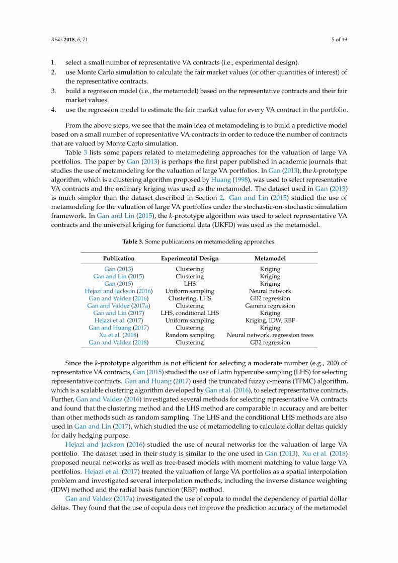
Table 3 lists some papers related to metamodeling approaches for the valuation of large VAportfolios. The paper by Gan (2013) is perhaps the first paper published in academic journals thatstudies the use of metamodeling for the valuation of large VA portfolios. In Gan (2013), the k-prototypealgorithm, which is a clustering algorithm proposed by Huang (1998), was used to select representativeVA contracts and the ordinary kriging was used as the metamodel. The dataset used in Gan (2013)is much simpler than the dataset described in Section 2. Gan and Lin (2015) studied the use ofmetamodeling for the valuation of large VA portfolios under the stochastic-on-stochastic simulationframework. In Gan and Lin (2015), the k-prototype algorithm was used to select representative VAcontracts and the universal kriging for functional data (UKFD) was used as the metamodel.

Table 3. Some publications on metamodeling approaches.

Publication Experimental Design Metamodel

Gan (2013) Clustering KrigingGan and Lin (2015) Clustering Kriging

Gan (2015) LHS KrigingHejazi and Jackson (2016) Uniform sampling Neural network

Gan and Valdez (2016) Clustering, LHS GB2 regressionGan and Valdez (2017a) Clustering Gamma regression

Gan and Lin (2017) LHS, conditional LHS KrigingHejazi et al. (2017) Uniform sampling Kriging, IDW, RBF

Gan and Huang (2017) Clustering KrigingXu et al. (2018) Random sampling Neural network, regression trees

Gan and Valdez (2018) Clustering GB2 regression

Since the k-prototype algorithm is not efficient for selecting a moderate number (e.g., 200) ofrepresentative VA contracts, Gan (2015) studied the use of Latin hypercube sampling (LHS) for selectingrepresentative contracts. Gan and Huang (2017) used the truncated fuzzy c-means (TFMC) algorithm,which is a scalable clustering algorithm developed by Gan et al. (2016), to select representative contracts.Further, Gan and Valdez (2016) investigated several methods for selecting representative VA contractsand found that the clustering method and the LHS method are comparable in accuracy and are betterthan other methods such as random sampling. The LHS and the conditional LHS methods are alsoused in Gan and Lin (2017), which studied the use of metamodeling to calculate dollar deltas quicklyfor daily hedging purpose.

Hejazi and Jackson (2016) studied the use of neural networks for the valuation of large VAportfolio. The dataset used in their study is similar to the one used in Gan (2013). Xu et al. (2018)proposed neural networks as well as tree-based models with moment matching to value large VAportfolios. Hejazi et al. (2017) treated the valuation of large VA portfolios as a spatial interpolationproblem and investigated several interpolation methods, including the inverse distance weighting(IDW) method and the radial basis function (RBF) method.

Gan and Valdez (2017a) investigated the use of copula to model the dependency of partial dollardeltas. They found that the use of copula does not improve the prediction accuracy of the metamodel

Risks 2018, 6, 71 6 of 19

because the dependency is well captured by the covariates. To address the skewness typically observedin the distribution of the fair market values, Gan and Valdez (2018) proposed the use of the generalizedbeta of the second kind (GB2) distribution to model the fair market values. Gan and Huang (2017)proposed a data mining framework for the valuation of large VA portfolios.

In all the work mentioned above, the interactions between the variables are not considered in themetamodels. In addition, some of the metamodels (e.g., kriging, neural networks, GB2 regression) arequite sophisticated. Fitting such metamodels poses challenges. As reported in Gan and Valdez (2018),for example, fitting GB2 regression models to the VA data is not straightforward and requires amulti-stage optimization procedure.

4. Learning Interactions

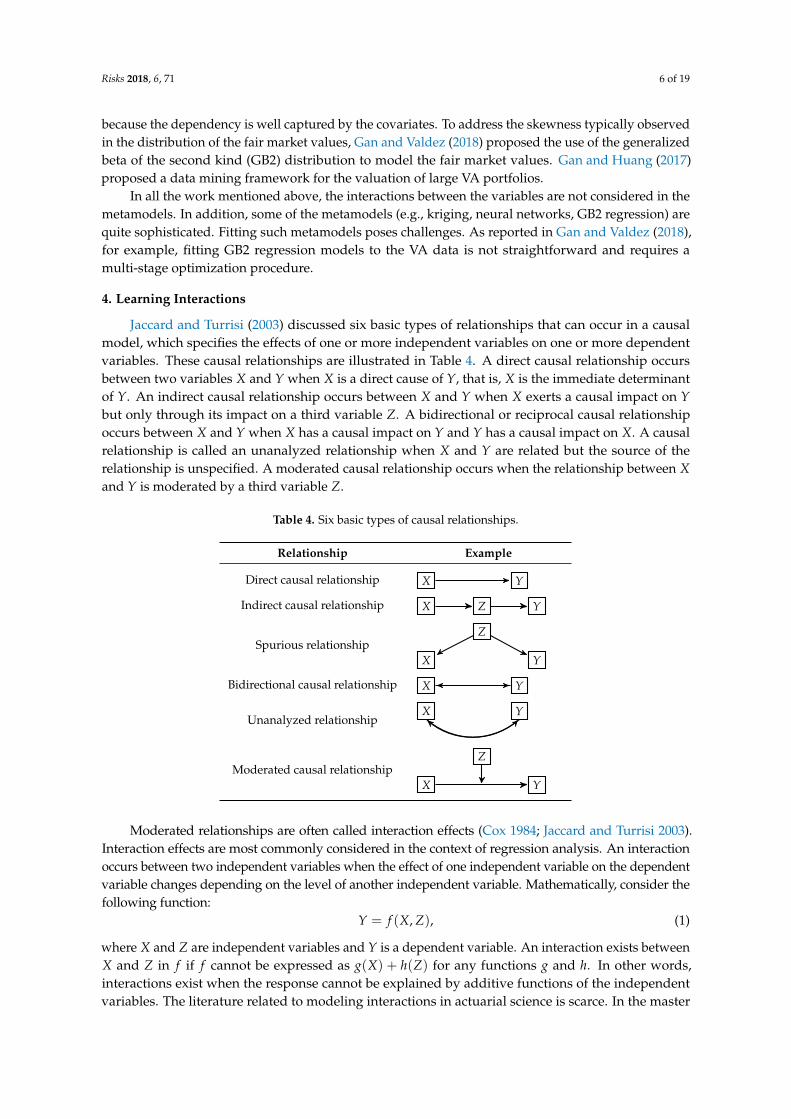
Jaccard and Turrisi (2003) discussed six basic types of relationships that can occur in a causalmodel, which specifies the effects of one or more independent variables on one or more dependentvariables. These causal relationships are illustrated in Table 4. A direct causal relationship occursbetween two variables X and Y when X is a direct cause of Y, that is, X is the immediate determinantof Y. An indirect causal relationship occurs between X and Y when X exerts a causal impact on Ybut only through its impact on a third variable Z. A bidirectional or reciprocal causal relationshipoccurs between X and Y when X has a causal impact on Y and Y has a causal impact on X. A causalrelationship is called an unanalyzed relationship when X and Y are related but the source of therelationship is unspecified. A moderated causal relationship occurs when the relationship between Xand Y is moderated by a third variable Z.

Table 4. Six basic types of causal relationships.

Relationship Example

Direct causal relationship X Y

Indirect causal relationship X Z Y

Spurious relationshipZ

X Y

Bidirectional causal relationship X Y

Unanalyzed relationshipX Y

Moderated causal relationshipZ

X Y

Moderated relationships are often called interaction effects (Cox 1984; Jaccard and Turrisi 2003).Interaction effects are most commonly considered in the context of regression analysis. An interactionoccurs between two independent variables when the effect of one independent variable on the dependentvariable changes depending on the level of another independent variable. Mathematically, consider thefollowing function:

Y = f (X, Z), (1)

where X and Z are independent variables and Y is a dependent variable. An interaction exists betweenX and Z in f if f cannot be expressed as g(X) + h(Z) for any functions g and h. In other words,interactions exist when the response cannot be explained by additive functions of the independentvariables. The literature related to modeling interactions in actuarial science is scarce. In the master

Risks 2018, 6, 71 7 of 19

thesis, Nawar (2016) investigated learning pairwise interactions in the Poisson and Gamma regressionmodels for P&C insurance.

Let Y be a continuous response variable. Let X1, X2, . . ., Xp be p explanatory variables,which include continuous and categorical variables. The the first-order interaction model is givenby (Lim and Hastie 2015):

E[Y|X1, X2, . . . , Xp] = β0 +p

∑j=1

β jXj + ∑s<t

βs:tXs:t, (2)

where the term Xs:t = XsXt denotes the interaction effect between Xs and Xt and terms X1, X2, . . ., Xp

denote the main effects. The interaction model is said to satisfy strong hierarchy if an interaction canexist only if both its main effects are present. The interaction model is said to satisfy weak hierarchy ifan interaction can exist as long as either of its main effects is present. Main effects can be viewed asdeviations from the global mean and interaction effects can be viewed as deviations from the maineffects. As a result, it rarely makes sense to have interactions without main effects. This means thathierarchical interaction models are usually preferred.

From Equation (2), we see that the first-order interaction model is an extension of the multiplelinear regression model by adding some interaction terms. One major advantage of adding theinteraction terms is that it helps increase the predictive power.

However, learning interactions is a challenging problem, especially when there are many variables.For example, the number of pairwise interaction terms among 20 variables is 20× 19/2 = 190, whichmay exceed the number of training samples. If we include all the pairwise interaction terms in theregression model, then the resulting model may overfit the data. To avoid the overfitting problem,we need to select important interactions only. However, selecting important interactions from a largenumber of interactions manually is a tedious task.

To address the aforementioned challenges, we use the overlapped group-lasso proposed byLim and Hastie (2015) that can produce hierarchical interaction models automatically. The overlappedgroup-lasso is based on the group-lasso proposed by Yuan and Lin (2006) by adding an overlappedgroup-lasso penalty. In the following subsections, we give a brief introduction of the group-lasso andthe overlapped group-lasso.

4.1. Group-Lasso

The group-lasso can be viewed as a general version of the popular lasso proposed byTibshirani (1996). Let y = (y1, y2, . . . , yn)′ denote the vector of responses and let X denote the designmatrix. Then the lasso is defined as

βLASSO

= arg minβ

(12‖y− Xβ‖2

2 + λ‖β‖1

), (3)

where ‖ · ‖2 denotes the `2-norm, ‖ · ‖1 denotes the `1-norm, and λ is a tuning parameter thatcontrols the amount of regularization. The `1-norm induces sparsity in the solution in the sensethat it sets some coefficients to zero. A larger value of λ implies more regularization. The lassosolution is piecewise linear with respect to the tuning parameter λ. The least angle regression selection(LARS) (Efron et al. 2004) is an efficient algorithm to solve the optimization problem in Equation (3)for all λ ∈ [0, ∞]. The final value of λ can be selected by techniques such as cross-validation.

The lasso is designed for selecting individual input variables but not for general factor selection.Yuan and Lin (2006) proposed group-lasso that aims to select important factors. Suppose that there are

Risks 2018, 6, 71 8 of 19

p groups of variables. For j = 1, 2, . . . , p, let Xj denote the feature matrix for group j. The group-lassocan be formulated as follows:

βGLASSO

= arg minβ

(12‖y− β01−

p

∑j=1

Xjβj‖22 + λ

p

∑j=1

γj‖βj‖2

), (4)

where 1 is a vector of ones, ‖ · ‖2 denotes the `2-norm, and λ, γ1, . . . , γp are tuning parameters.The parameter λ controls the overall amount of regularization while the parameters γ1, . . . , γp alloweach group to be penalized to different extents. When each group contains one continuous variable,the group-lasso reduces to the lasso. Like the lasso, the penalty on coefficients will force some βj to

be zero. An attractive property of the group-lasso is that if βj is nonzero, then all its components aretypically nonzero.

The optimization problem in Equation (4) can be solved by starting with a value of λ that is justlarge enough to make all estimates zero. Then a path of solutions can be obtained by decreasing λ

along a grid of values. An optimal λ can be chosen by cross-validation.

4.2. Overlapped Group-Lasso

The overlapped group-lasso extends the group-lasso by adding an overlapped group-lasso penaltyto the loss function in order to obtain hierarchical interaction models. The overlapped group-lasso isformulated as the following constrained optimization problem (Lim and Hastie 2015):

βOGLASSO

= arg minβ

(12

∥∥∥y− β01−∑pj=1 Xjβj −∑s<t(Xs βs + Xt βt + Xs:tβs:t)

∥∥∥2

2

+λ

(∑

pj=1 ‖βj‖2 + ∑s<t

√Ls‖βs‖2

2 + Lt‖βt‖22 + ‖βs:t‖2

2

)),

(5)

subject to the following sets of constraints:∑

mjl=1 β

(l)j = 0, ∑

mjl=1 β

(l)j = 0, if Xj is categorical;

∑mjl=1 β

(l)t:j = 0, if Xj is categorical and Xt is continuous;

∑mjl=1 β

(l,k)t:j = 0 ∀k, ∑mt

k=1 β(l,k)t:j = 0 ∀l, if Xj and Xt are categorical,

(6)

where mj is the number of levels of Xj, mt is the number of levels of Xt, β(l)j is the lth entry of βj, β

(l)j is

the lth entry of βj, and β(l,k)t:j is the lkth entry of βt:j. The constants Ls and Lt are selected such that βs,

βt, and βs:t are on the same scale.In Equation (5), X1, X2, . . ., Xp denote the feature matrices of the p group of variables,

X1, X2, . . ., Xp, which include continuous and categorical variables. If Xj is continuous, then Xjis just a one-column matrix containing the values of Xj, that is,

Xj = (x1j, x2j, . . . , xnj)′, (7)

where n is the number of observations and xij is the value of Xj in the ith observation. If Xj iscategorical, then Xj contains all the dummy variables associated with Xj. For example, if Xj has mjlevels, then Xj is an n × mj indicator matrix where the (i, l)-entry is 1 if the value of Xj in the ithobservation is equal to the lth level; otherwise, the (i, l)-entry is zero.

Risks 2018, 6, 71 9 of 19

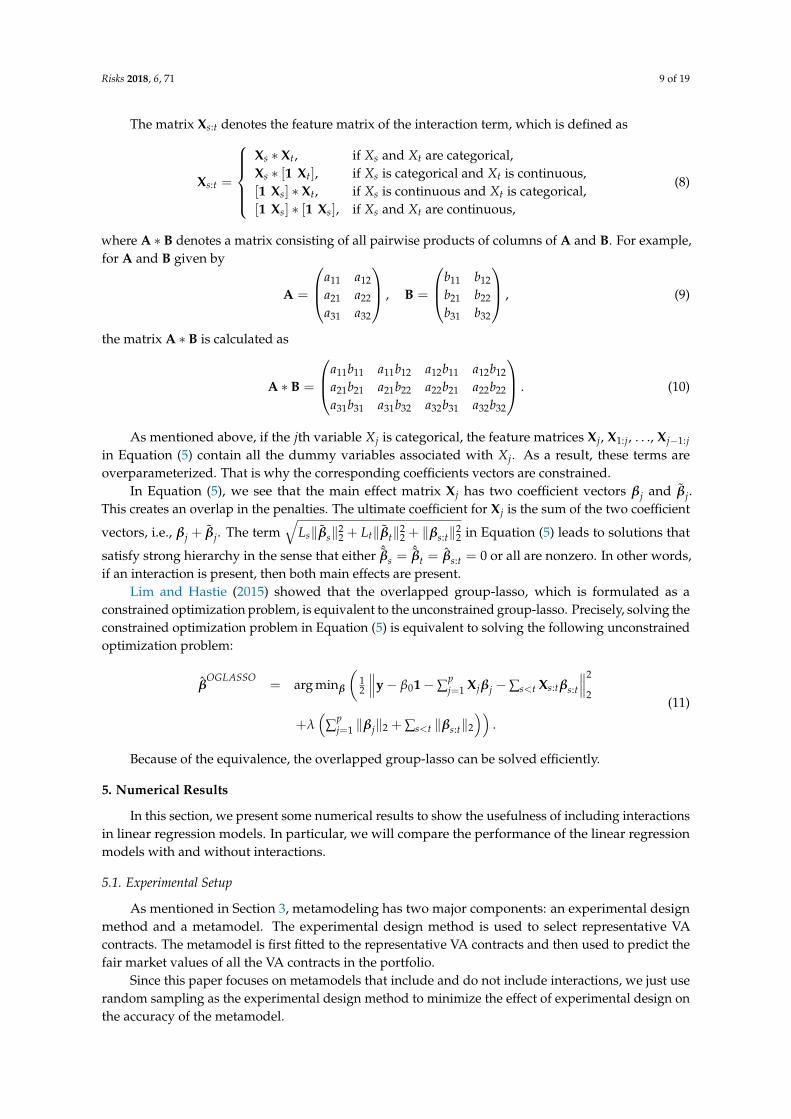
The matrix Xs:t denotes the feature matrix of the interaction term, which is defined as

Xs:t =

Xs ∗ Xt, if Xs and Xt are categorical,Xs ∗ [1 Xt], if Xs is categorical and Xt is continuous,[1 Xs] ∗ Xt, if Xs is continuous and Xt is categorical,[1 Xs] ∗ [1 Xs], if Xs and Xt are continuous,

(8)

where A ∗ B denotes a matrix consisting of all pairwise products of columns of A and B. For example,for A and B given by

A =

a11 a12

a21 a22

a31 a32

, B =

b11 b12

b21 b22

b31 b32

, (9)

the matrix A ∗ B is calculated as

A ∗ B =

a11b11 a11b12 a12b11 a12b12

a21b21 a21b22 a22b21 a22b22

a31b31 a31b32 a32b31 a32b32

. (10)

As mentioned above, if the jth variable Xj is categorical, the feature matrices Xj, X1:j, . . ., Xj−1:jin Equation (5) contain all the dummy variables associated with Xj. As a result, these terms areoverparameterized. That is why the corresponding coefficients vectors are constrained.

In Equation (5), we see that the main effect matrix Xj has two coefficient vectors βj and βj.This creates an overlap in the penalties. The ultimate coefficient for Xj is the sum of the two coefficient

vectors, i.e., βj + βj. The term√

Ls‖βs‖22 + Lt‖βt‖2

2 + ‖βs:t‖22 in Equation (5) leads to solutions that

satisfy strong hierarchy in the sense that either ˆβs =ˆβt = βs:t = 0 or all are nonzero. In other words,

if an interaction is present, then both main effects are present.Lim and Hastie (2015) showed that the overlapped group-lasso, which is formulated as a

constrained optimization problem, is equivalent to the unconstrained group-lasso. Precisely, solving theconstrained optimization problem in Equation (5) is equivalent to solving the following unconstrainedoptimization problem:

βOGLASSO

= arg minβ

(12

∥∥∥y− β01−∑pj=1 Xjβj −∑s<t Xs:tβs:t

∥∥∥2

2

+λ(

∑pj=1 ‖βj‖2 + ∑s<t ‖βs:t‖2

)).

(11)

Because of the equivalence, the overlapped group-lasso can be solved efficiently.

5. Numerical Results

In this section, we present some numerical results to show the usefulness of including interactionsin linear regression models. In particular, we will compare the performance of the linear regressionmodels with and without interactions.

5.1. Experimental Setup

As mentioned in Section 3, metamodeling has two major components: an experimental designmethod and a metamodel. The experimental design method is used to select representative VAcontracts. The metamodel is first fitted to the representative VA contracts and then used to predict thefair market values of all the VA contracts in the portfolio.

Since this paper focuses on metamodels that include and do not include interactions, we just userandom sampling as the experimental design method to minimize the effect of experimental design onthe accuracy of the metamodel.

Risks 2018, 6, 71 10 of 19

Another important factor to consider in metamodeling is the number of representative VAcontracts. There is a trade-off between accuracy and speed. If only a few representative VA contractsare used, then it takes less time to run Monte Carlo valuation for the representative VA contracts.However, the fitted metamodel might not be accurate. If a lot of representative VA contracts areused, then the fitted metamodel performs well in terms of prediction accuracy. However, in thiscase it takes more time to run Monte Carlo simulation. In this paper, we follow the strategy usedin previous studies (e.g., Gan and Lin 2015) to determine the number of representative VA contracts,that is, we use 10 times the number of predictors, including the dummy variables converted fromcategorical variables. Since there are 34 predictors, we start with 340 representative VA contracts.We also use 680 representative VA contracts to see the impact of the number of representative VAcontracts on the performance of the metamodels.

To fit linear models to the data, we use the R function lm from the stats package. To fit theoverlapped group-lasso, we use the R function glinternet.cv with default settings from the glinternetpackage developed by Lim and Hastie (2018). We use 10-fold cross-validation to select the best valueof λ in Equation (5).

5.2. Validation Measures

To compare the prediction accuracy of the metamodels, we use the following three validationmeasures: the percentage error at the portfolio level, the R2 (Frees 2009), and the concordancecorrelation coefficient (Lin 1989).

Let yi denote the fair market value of the ith VA policy in the portfolio that is calculated by MonteCarlo simulation method. Let yi denote the fair market value predicted by a metamodel. Then thepercentage error (PE) at the portfolio level is defined as

PE =

n∑

i=1(yi − yi)

n∑

i=1yi

, (12)

where n is the number of VA policies in the portfolio. Between two metamodels, the one producing aPE that is closer to zero is better.

The R2 is calculated as

R2 = 1−

n∑

i=1(yi − yi)

2

n∑

i=1(yi − y)2

, (13)

where y is the average of y1, y2, . . . , yn. Between two metamodels, the one that produces a lower MSEis better.

The concordance correlation coefficient (CCC) is used to measure the agreement between twovariables. It is defined as follows (Lin 1989):

CCC =2ρσ1σ2

σ21 + σ2

2 + (µ1 − µ2)2. (14)

where ρ is the correlation between (y1, y2, . . . , yn) and (y1, y2, . . . , yn), σ1 and µ1 are the standarddeviation and the mean of (y1, y2, . . . , yn), respectively, and σ2 and µ2 are the standard deviation andthe mean of (y1, y2, . . ., yn), respectively. Between two metamodels, the one that produces a higherCCC is considered a better model. In particular, a value of 1 indicates perfect agreement between thetwo models.

Risks 2018, 6, 71 11 of 19

5.3. Results

To demonstrate the benefit of including interactions in regression models, we fitted a multiplelinear regression model without interactions and the first-order interaction model defined inEquation (2) to the representative VA contracts. We conducted our experiments on a Laptop computerwith a Windows operating system and 8 GB memory.

Table 5 shows the values of the validation measures for the linear models with and withoutinteractions when 340 representative VA contracts were used. All the validation measures show thatthe linear model with interactions outperformed the one without interactions in terms of accuracy.At the portfolio level, for example, the percentage error of the linear model with interactions is around−0.4%, while the percentage error of the linear model without interactions is around 2.1%, whichis higher. Since we used 10-fold cross validation to select the optimal tuning parameter λ in theoverlapped group-lasso, the runtime used to fit the linear model with interactions is higher.

Table 5. Accuracy and runtime of the metamodels when 340 representative VA contracts were used.The runtime is in seconds.

Model PE R2 CCC Runtime

Linear Model without interactions 0.0207 0.7986 0.8957 0.2700Linear Model with interactions −0.0036 0.9441 0.9697 37.8900

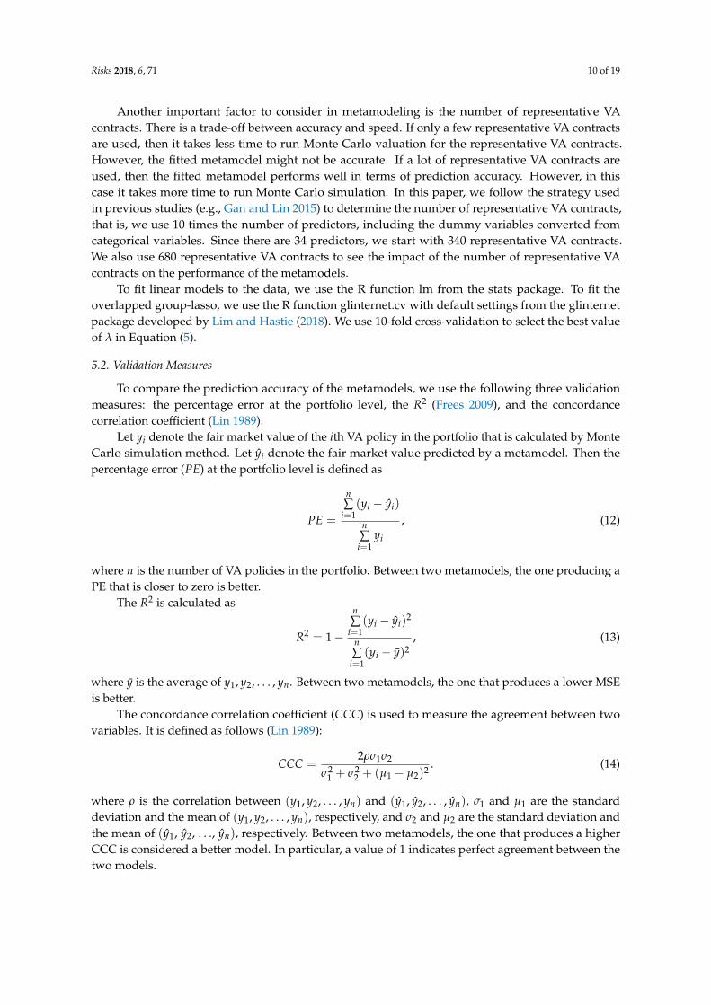
Figure 3 shows the scatter plots between the fair market values calculated by Monte Carlo andthose predicted by the linear models with and without interactions when 340 representative VAcontracts were used. The figures show that the linear model without interactions did not fit the tailswell. For example, many of the contracts have near zero fair market values. However, their fair marketvalues predicted by the linear model without interactions ranges from less than −$500 thousand tonear $500 thousand. Table 6 shows some summary statistics of the prediction errors of individual VAcontracts. From the table, we see that prediction errors of the linear model with interactions have amore symmetric distribution.

(a) (b)

Figure 3. Scatter plots of the fair market values calculated by Monte Carlo simulation and thosepredicted by linear models when 340 representative VA contracts were used. The numbers are inthousands. (a) Without interactions; (b) With interactions.

Risks 2018, 6, 71 12 of 19

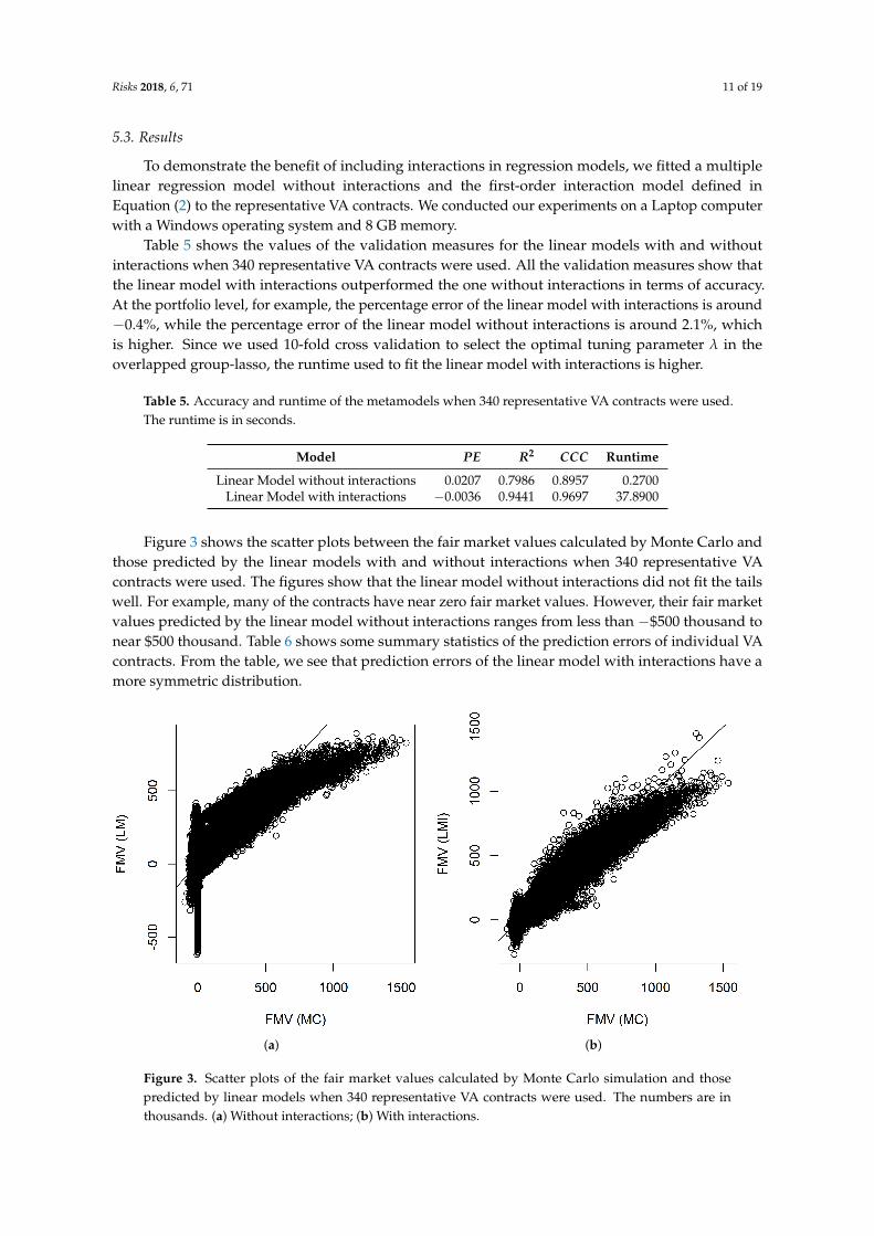
Figure 4 shows the QQ plots produced by the linear model with interactions found by theoverlapped group-lasso and the linear model without interactions. If we look at these plots, we seethat the linear model with interactions worked pretty well, although the fitting at the tails is a littlebit off.

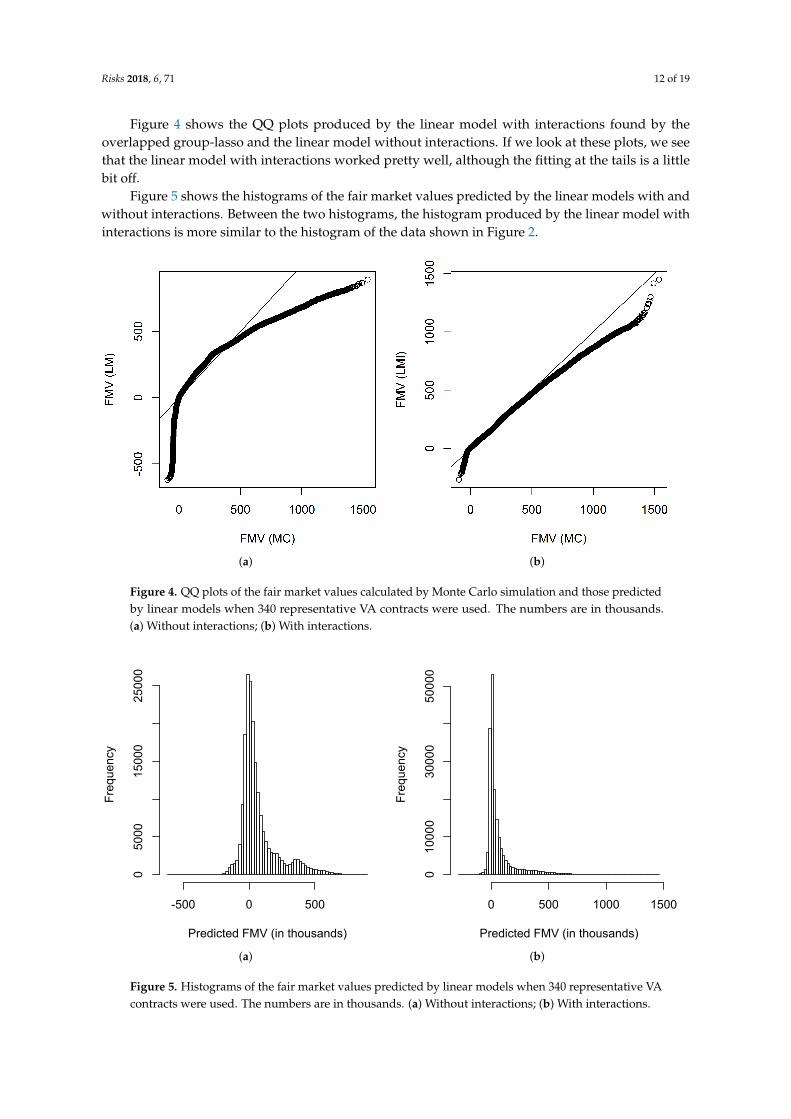
Figure 5 shows the histograms of the fair market values predicted by the linear models with andwithout interactions. Between the two histograms, the histogram produced by the linear model withinteractions is more similar to the histogram of the data shown in Figure 2.

(a) (b)

Figure 4. QQ plots of the fair market values calculated by Monte Carlo simulation and those predictedby linear models when 340 representative VA contracts were used. The numbers are in thousands.(a) Without interactions; (b) With interactions.

Predicted FMV (in thousands)

Frequency

-500 0 500

05000

15000

25000

(a)

Predicted FMV (in thousands)

Frequency

0 500 1000 1500

010000

30000

50000

(b)

Figure 5. Histograms of the fair market values predicted by linear models when 340 representative VAcontracts were used. The numbers are in thousands. (a) Without interactions; (b) With interactions.

Risks 2018, 6, 71 13 of 19

Table 6. Summary statistics of the prediction errors of individual VA contracts when 340 representativeVA contracts were used.

Model Min 1st Q Median Mean 3rd Q Max

Linear Model without interactions −432.13 −28.46 1.08 −1.40 25.97 708.65Linear Model with interactions −515.96 −12.23 −2.25 0.10 7.57 478.52

If we compare Figures 3b, 4b and 5b to Figures 3a, 4a and 5a, we can see that the improvementthat resulted from including interactions is significant.

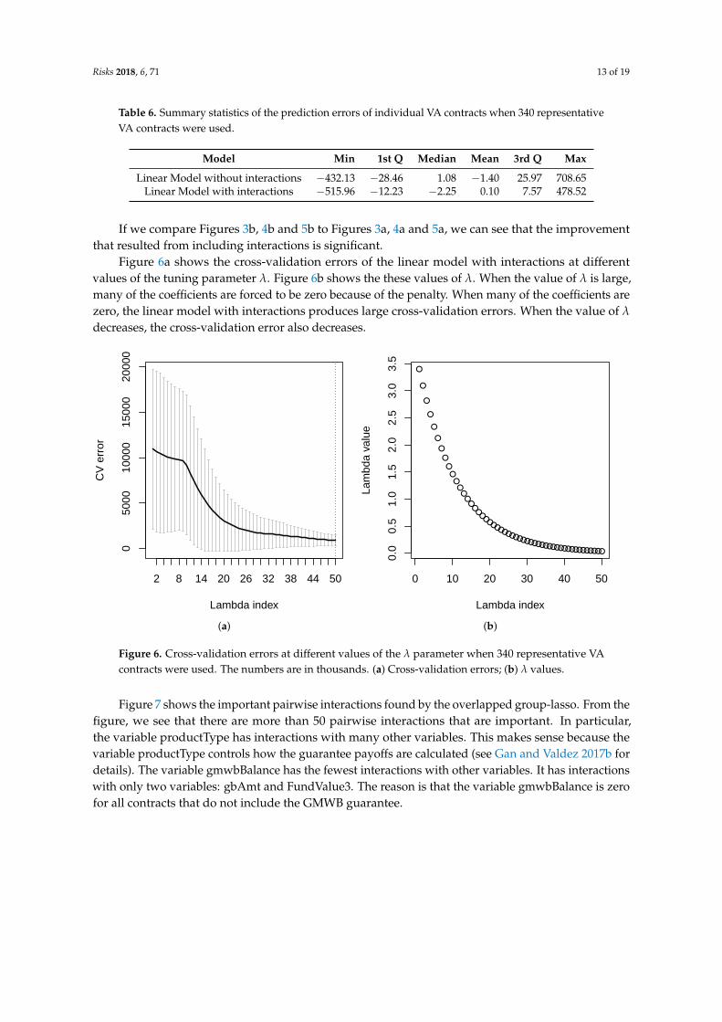
Figure 6a shows the cross-validation errors of the linear model with interactions at differentvalues of the tuning parameter λ. Figure 6b shows the these values of λ. When the value of λ is large,many of the coefficients are forced to be zero because of the penalty. When many of the coefficients arezero, the linear model with interactions produces large cross-validation errors. When the value of λ

decreases, the cross-validation error also decreases.

050

0010

000

1500

020

000

Lambda index

CV

err

or

2 8 14 20 26 32 38 44 50

(a)

●

●

●

●

●

●

●

●

●●●●●●●●●●●●●●●●●●●●●●●●●●●●●●●●●●●●●●●●●●

0 10 20 30 40 50

0.0

0.5

1.0

1.5

2.0

2.5

3.0

3.5

Lambda index

Lam

bda

valu

e

(b)

Figure 6. Cross-validation errors at different values of the λ parameter when 340 representative VAcontracts were used. The numbers are in thousands. (a) Cross-validation errors; (b) λ values.

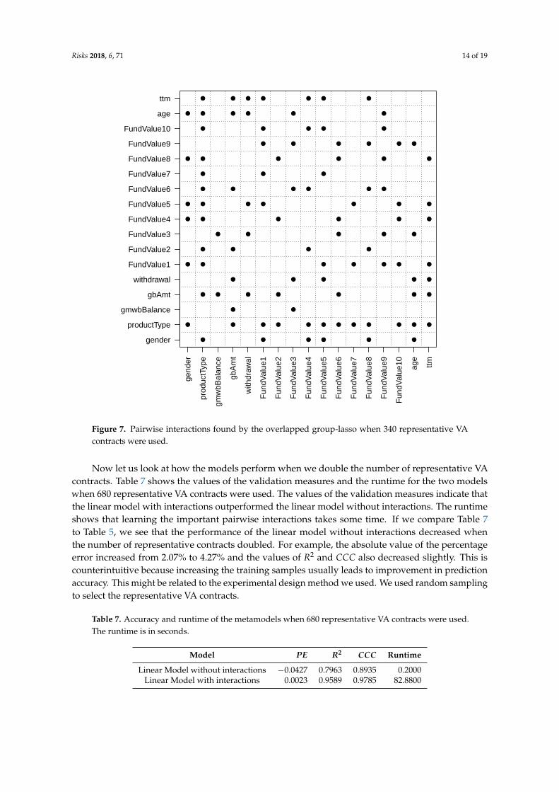
Figure 7 shows the important pairwise interactions found by the overlapped group-lasso. From thefigure, we see that there are more than 50 pairwise interactions that are important. In particular,the variable productType has interactions with many other variables. This makes sense because thevariable productType controls how the guarantee payoffs are calculated (see Gan and Valdez 2017b fordetails). The variable gmwbBalance has the fewest interactions with other variables. It has interactionswith only two variables: gbAmt and FundValue3. The reason is that the variable gmwbBalance is zerofor all contracts that do not include the GMWB guarantee.

Risks 2018, 6, 71 14 of 19

gend

er

prod

uctT

ype

gmw

bBal

ance

gbA

mt

with

draw

al

Fun

dVal

ue1

Fun

dVal

ue2

Fun

dVal

ue3

Fun

dVal

ue4

Fun

dVal

ue5

Fun

dVal

ue6

Fun

dVal

ue7

Fun

dVal

ue8

Fun

dVal

ue9

Fun

dVal

ue10 age

ttm

gender

productType

gmwbBalance

gbAmt

withdrawal

FundValue1

FundValue2

FundValue3

FundValue4

FundValue5

FundValue6

FundValue7

FundValue8

FundValue9

FundValue10

age

ttm

●

●

●

●

●

●

●

●

●

●

●

●

●

●

●

●

●

●

●

●

●

●

●

●

●

●

●

●

●

●

●

●

●

●

●

●

●

●

●

●

●

●

●

●

●

●

●

●

●

●

●

●

●

●

●

●

●

●

●

●

●

●

●

●

●

●

●

●

●

●

●

●

●

●

●

●

●

●

●

●

●

●

●

●

●

●

●

●

●

●

●

●

●

●

●

●

●

●

●

●

Figure 7. Pairwise interactions found by the overlapped group-lasso when 340 representative VAcontracts were used.

Now let us look at how the models perform when we double the number of representative VAcontracts. Table 7 shows the values of the validation measures and the runtime for the two modelswhen 680 representative VA contracts were used. The values of the validation measures indicate thatthe linear model with interactions outperformed the linear model without interactions. The runtimeshows that learning the important pairwise interactions takes some time. If we compare Table 7to Table 5, we see that the performance of the linear model without interactions decreased whenthe number of representative contracts doubled. For example, the absolute value of the percentageerror increased from 2.07% to 4.27% and the values of R2 and CCC also decreased slightly. This iscounterintuitive because increasing the training samples usually leads to improvement in predictionaccuracy. This might be related to the experimental design method we used. We used random samplingto select the representative VA contracts.

Table 7. Accuracy and runtime of the metamodels when 680 representative VA contracts were used.The runtime is in seconds.

Model PE R2 CCC Runtime

Linear Model without interactions −0.0427 0.7963 0.8935 0.2000Linear Model with interactions 0.0023 0.9589 0.9785 82.8800

Risks 2018, 6, 71 15 of 19

If we compare the values of the validation measures for the linear model with interactions inTables 5 and 7, we see that the accuracy of the linear model with interactions increased when wedoubled the number of representative VA contracts. For example, the absolute value of the percentageerror decreased from 0.36% to 0.23%, the R2 increased from 0.9441 to 0.9589, and the CCC increasedfrom 0.9697 to 0.9785. The validation measures show that the impact of experimental design is notmaterial when interactions are included. If we use a higher number of representative VA contracts,however, the runtime will increase due to the cross-validation.

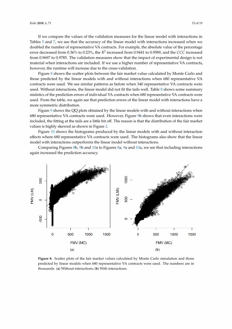
Figure 8 shows the scatter plots between the fair market value calculated by Monte Carlo andthose predicted by the linear models with and without interactions when 680 representative VAcontracts were used. We see similar patterns as before when 340 representative VA contracts wereused. Without interactions, the linear model did not fit the tails well. Table 8 shows some summarystatistics of the prediction errors of individual VA contracts when 680 representative VA contracts wereused. From the table, we again see that prediction errors of the linear model with interactions have amore symmetric distribution.

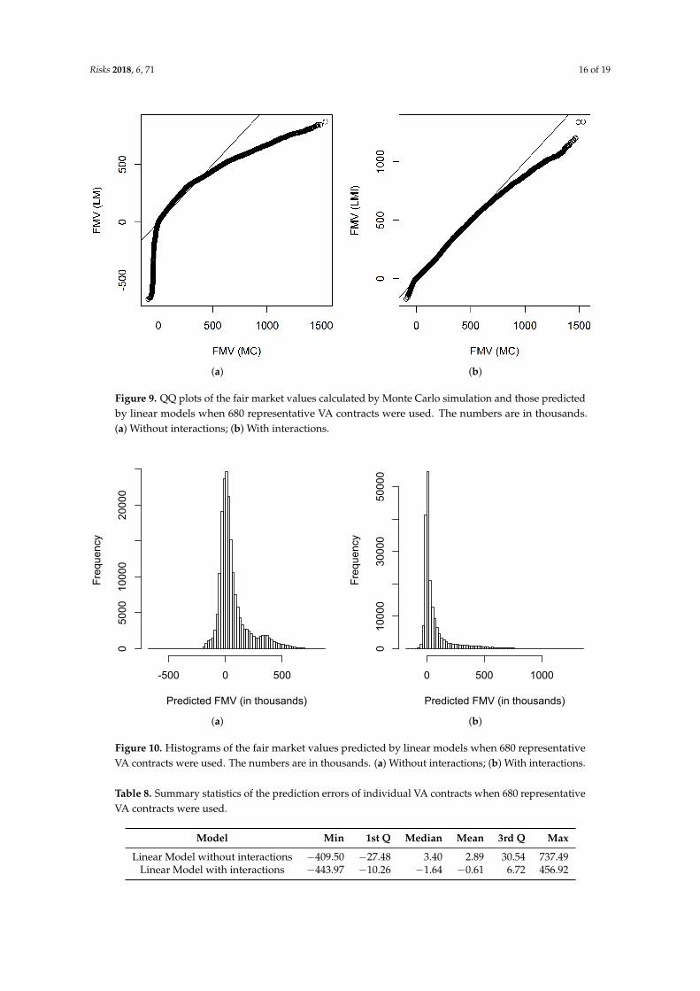
Figure 9 shows the QQ plots obtained by the linear models with and without interactions when680 representative VA contracts were used. However, Figure 9b shows that even interactions wereincluded, the fitting at the tails are a little bit off. The reason is that the distribution of the fair marketvalues is highly skewed as shown in Figure 2.

Figure 10 shows the histograms produced by the linear models with and without interactioneffects where 680 representative VA contracts were used. The histograms also show that the linearmodel with interactions outperforms the linear model without interactions.

Comparing Figures 8b, 9b and 10a to Figures 8a, 9a and 10a, we see that including interactionsagain increased the prediction accuracy.

(a) (b)

Figure 8. Scatter plots of the fair market values calculated by Monte Carlo simulation and thosepredicted by linear models when 680 representative VA contracts were used. The numbers are inthousands. (a) Without interactions; (b) With interactions.

Risks 2018, 6, 71 16 of 19

(a) (b)

Figure 9. QQ plots of the fair market values calculated by Monte Carlo simulation and those predictedby linear models when 680 representative VA contracts were used. The numbers are in thousands.(a) Without interactions; (b) With interactions.

Predicted FMV (in thousands)

Frequency

-500 0 500

05000

10000

20000

(a)

Predicted FMV (in thousands)

Frequency

0 500 1000

010000

30000

50000

(b)

Figure 10. Histograms of the fair market values predicted by linear models when 680 representativeVA contracts were used. The numbers are in thousands. (a) Without interactions; (b) With interactions.

Table 8. Summary statistics of the prediction errors of individual VA contracts when 680 representativeVA contracts were used.

Model Min 1st Q Median Mean 3rd Q Max

Linear Model without interactions −409.50 −27.48 3.40 2.89 30.54 737.49Linear Model with interactions −443.97 −10.26 −1.64 −0.61 6.72 456.92

Risks 2018, 6, 71 17 of 19

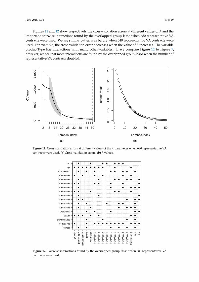
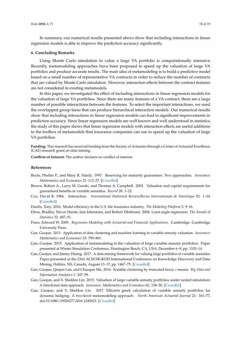
Figures 11 and 12 show respectively the cross-validation errors at different values of λ and theimportant pairwise interactions found by the overlapped group-lasso when 680 representative VAcontracts were used. We see similar patterns as before when 340 representative VA contracts wereused. For example, the cross-validation error decreases when the value of λ increases. The variableproductType has interactions with many other variables. If we compare Figure 12 to Figure 7,however, we see that more interactions are found by the overlapped group-lasso when the number ofrepresentative VA contracts doubled.

050

0010

000

1500

0

Lambda index

CV

err

or

2 8 14 20 26 32 38 44 50

(a)

●

●

●

●

●

●

●

●

●●●●●●●●●●●●●●●●●●●●●●●●●●●●●●●●●●●●●●●●●●

0 10 20 30 40 50

0.0

0.5

1.0

1.5

2.0

2.5

Lambda index

Lam

bda

valu

e

(b)

Figure 11. Cross-validation errors at different values of the λ parameter when 680 representative VAcontracts were used. (a) Cross-validation errors; (b) λ values.

gend

er

prod

uctT

ype

gmw

bBal

ance

gbA

mt

with

draw

al

Fun

dVal

ue1

Fun

dVal

ue2

Fun

dVal

ue3

Fun

dVal

ue4

Fun

dVal

ue5

Fun

dVal

ue6

Fun

dVal

ue7

Fun

dVal

ue8

Fun

dVal

ue9

Fun

dVal

ue10 age

ttm

gender

productType

gmwbBalance

gbAmt

withdrawal

FundValue1

FundValue2

FundValue3

FundValue4

FundValue5

FundValue6

FundValue7

FundValue8

FundValue9

FundValue10

age

ttm

●

●

●

●

●

●

●

●

●

●

●

●

●

●

●

●

●

●

●

●

●

●

●

●

●

●

●

●

●

●

●

●

●

●

●

●

●

●

●

●

●

●

●

●

●

●

●

●

●

●

●

●

●

●

●

●

●

●

●

●

●

●

●

●

●

●

●

●

●

●

●

●

●

●

●

●

●

●

●

●

●

●

●

●

●

●

●

●

●

●

●

●

●

●

●

●

●

●

●

●

●

●

●

●

●

●

●

●

●

●

●

●

Figure 12. Pairwise interactions found by the overlapped group-lasso when 680 representative VAcontracts were used.

Risks 2018, 6, 71 18 of 19

In summary, our numerical results presented above show that including interactions in linearregression models is able to improve the prediction accuracy significantly.

6. Concluding Remarks

Using Monte Carlo simulation to value a large VA portfolio is computationally intensive.Recently, metamodeling approaches have been proposed to speed up the valuation of large VAportfolios and produce accurate results. The main idea of metamodeling is to build a predictive modelbased on a small number of representative VA contracts in order to reduce the number of contractsthat are valued by Monte Carlo simulation. However, interaction effects between the contract featuresare not considered in existing metamodels.

In this paper, we investigated the effect of including interactions in linear regression models forthe valuation of large VA portfolios. Since there are many features of a VA contract, there are a largenumber of possible interactions between the features. To select the important interactions, we usedthe overlapped group-lasso that can produce hierarchical interaction models. Our numerical resultsshow that including interactions in linear regression models can lead to significant improvements inprediction accuracy. Since linear regression models are well known and well understood in statistics,the study of this paper shows that linear regression models with interaction effects are useful additionsto the toolbox of metamodels that insurance companies can use to speed up the valuation of largeVA portfolios.

Funding: This research has received funding from the Society of Actuaries through a Center of Actuarial Excellence(CAE) research grant on data mining.

Conflicts of Interest: The author declares no conflict of interest.

References

Boyle, Phelim P., and Mary R. Hardy. 1997. Reserving for maturity guarantees: Two approaches. Insurance:Mathematics and Economics 21: 113–27. [CrossRef]

Brown, Robert A., Larry M. Gorski, and Thomas A. Campbell. 2002. Valuation and capital requirements forguaranteed benefits in variable annuities. Record 28: 1–22.

Cox, David R. 1984. Interaction. International Statistical Review/Revue Internationale de Statistique 52: 1–24.[CrossRef]

Dardis, Tony. 2016. Model efficiency in the U.S. life insurance industry. The Modeling Platform 3: 9–16.Efron, Bradley, Trevor Hastie, Iain Johnstone, and Robert Tibshirani. 2004. Least angle regression. The Annals of

Statistics 32: 407–51.Frees, Edward W. 2009. Regression Modeling with Actuarial and Financial Applications. Cambridge: Cambridge

University Press.Gan, Guojun. 2013. Application of data clustering and machine learning in variable annuity valuation. Insurance:

Mathematics and Economics 53: 795–801.Gan, Guojun. 2015. Application of metamodeling to the valuation of large variable annuity portfolios. Paper

presented at Winter Simulation Conference, Huntington Beach, CA, USA, December 6–9; pp. 1103–14.Gan, Guojun, and Jimmy Huang. 2017. A data mining framework for valuing large portfolios of variable annuities.

Paper presented at the 23rd ACM SIGKDD International Conference on Knowledge Discovery and DataMining, Halifax, NS, Canada, August 13–17; pp. 1467–75. [CrossRef]

Gan, Guojun, Qiujun Lan, and Chaoqun Ma. 2016. Scalable clustering by truncated fuzzy c-means. Big Data andInformation Analytics 1: 247–59.

Gan, Guojun, and X. Sheldon Lin. 2015. Valuation of large variable annuity portfolios under nested simulation:A functional data approach. Insurance: Mathematics and Economics 62: 138–50. [CrossRef]

Gan, Guojun, and X. Sheldon Lin. 2017. Efficient greek calculation of variable annuity portfolios fordynamic hedging: A two-level metamodeling approach. North American Actuarial Journal 21: 161–77,doi:10.1080/10920277.2016.1245623. [CrossRef]

Risks 2018, 6, 71 19 of 19

Gan, Guojun, and Emiliano A. Valdez. 2016. An empirical comparison of some experimental designs for thevaluation of large variable annuity portfolios. Dependence Modeling 4: 382–400. [CrossRef]

Gan, Guojun, and Emiliano A. Valdez. 2017a. Modeling partial greeks of variable annuities with dependence.Insurance: Mathematics and Econocmics 76: 118–34, doi:10.1016/j.insmatheco.2017.07.006. [CrossRef]

Gan, Guojun, and Emiliano A. Valdez. 2017b. Valuation of large variable annuity portfolios: Monte carlosimulation and synthetic datasets. Dependence Modeling 5: 354–74, doi:10.1515/demo-2017-0021. [CrossRef]

Gan, Guojun, and Emiliano A. Valdez. 2018. Regression modeling for the valuation of large variable annuityportfolios. North American Actuarial Journal 22: 40–54. [CrossRef]

Hardy, Mary. 2003. Investment Guarantees: Modeling and Risk Management for Equity-Linked Life Insurance. Hoboken:John Wiley & Sons, Inc.

Hejazi, Seyed Amir, and Kenneth R. Jackson. 2016. A neural network approach to efficient valuation of largeportfolios of variable annuities. Insurance: Mathematics and Economics 70: 169–81. [CrossRef]

Hejazi, Seyed Amir, Kenneth R. Jackson, and Guojun Gan. 2017. A spatial interpolation framework forefficient valuation of large portfolios of variable annuities. Quantitative Finance and Economics 1: 125–44,doi:10.3934/QFE.2017.2.125. [CrossRef]

Huang, Zhexue. 1998. Extensions to the k-means algorithm for clustering large data sets with categorical values.Data Mining and Knowledge Discovery 2: 283–304. [CrossRef]

Jaccard, James J., and Robert Turrisi. 2003. Interaction Effects in Multiple Regression, 2nd ed. Thousand Oaks:Sage Publications, Inc.

Ledlie, M. C., D. P. Corry, G. S. Finkelstein, A. J. Ritchie, K. Su, and D. C. E. Wilson. 2008. Variable annuities.British Actuarial Journal 14: 327–89. [CrossRef]

Lim, Michael, and Trevor Hastie. 2018. Learning Interactions via Hierarchical Group-Lasso Regularization. R PackageVersion 1.0.7.

Lim, Michael, and Trevor J. Hastie. 2015. Learning interactions via hierarchical group-lasso regularization.Journal of Computational and Graphical Statistics 24: 627–54. [CrossRef] [PubMed]

Lin, Lawrence I-Kuei. 1989. A concordance correlation coefficient to evaluate reproducibility. Biometrics 45:255–68. [CrossRef] [PubMed]

Nawar, Sandra Maria. 2016. Machine Learning Techniques for Detecting Hierarchical Interactions in InsuranceClaims Models. Master’s thesis, Concordia University, Montreal, QC, Canada.

The Geneva Association Report. 2013. Variable Annuities—An Analysis of Financial Stability. Available online:https://www.genevaassociation.org/sites/default/files/research-topics-document-type/pdf_public/ga2013-variable_annuities_0.pdf (accessed on 11 July 2018).

Tibshirani, Robert. 1996. Regression shrinkage and selection via the lasso. Journal of the Royal Statistical Society.Series B (Methodological) 58: 267–88.

Xu, Wei, Yuehuan Chen, Conrad Coleman, and Thomas F. Coleman. 2018. Moment matching machine learningmethods for risk management of large variable annuity portfolios. Journal of Economic Dynamics and Control 87:1–20. [CrossRef]

Yuan, Ming, and Yi Lin. 2006. Model selection and estimation in regression with grouped variables. Journal of theRoyal Statistical Society, Series B (Methodological) 68: 49–67. [CrossRef]

c© 2018 by the authors. Licensee MDPI, Basel, Switzerland. This article is an open accessarticle distributed under the terms and conditions of the Creative Commons Attribution(CC BY) license (http://creativecommons.org/licenses/by/4.0/).