vDESIGN OF URBAN DISTRIBUTION FEEDERS FOR VOLTAGE PROFILE IMPROVEMENT & DISTRIBUTION LOSSES REDUCTION

DESIGN OF URBAN DISTRIBUTION FEEDERS FOR VOLTAGEPROFILE IMPROVEMENT & DISTRIBUTION LOSSES REDUCTION

Ritula Thakur1 & Puneet Chawla 2

1.Astt. Prof. National Institute of Technical Teacher’s Training &Research, Sector-26, Chandigarh

2. Astt Prof. Electrical Engg. Dept., Ch. Devi Lal State Institute ofEngg. & Tech., Panniwala Mota (Sirsa)

ABSTRACT: India’s power sector is characterised by inadequateand inefficient power supply. Since the country’s independence,consumers are confronted with frequent power cuts, andfluctuating voltages and frequencies. In addition, system lossesare high throughout India Transmission and distributionnetworks. In addition to these enormous direct losses, theindirect losses in terms of lost productivity and trade, saggingeconomic activity, rapidly shrinking of domestic and foreigninvestment in the power sector, uneconomical and misallocatedinvestments in captive power, and reduced power generation couldbe many-fold. Distribution Sector requires economical system toprovide electrical energy at a suitable prize and at a minimumvoltage drop to reduce the voltage regulation. So, we requirethe economical way to provide the electrical energy by StateElectricity Boards to various consumers at minimum voltage dropand reduce the regulation of voltage. Calculations & analysiswill be required for load points, tie-points to selectrespective kVA capacity of transformers and hence theinstallation of suitable capacitor banks with proper locationsfor improvement of power factor and harmonics. This papersuggests the different methods of reduction of distributionlosses in the 11kV urban distribution feeder to improve thevoltage profile. Keywords: Distribution Sector, Punjab State Electricity Board,11kV urban distribution feeder, ACSR conductors, voltage drop,voltage profile, coefficient of temperature rise and modulus ofelasticity. I VOLTAGE DROP CALCULATION OF DISTRIBUTION FEEDERS

Distribution Sector requires economical system to provideelectrical energy at a suitable prize and at a minimum voltagedrop to reduce the voltage regulation. So, we require the

economical way to provide the electrical energy by StateElectricity Boards to various consumers at minimum voltage dropand reduce the regulation of voltage. The invisible energy whichconstitutes the flow of electrons on a closed circuit to do workis called electricity. Need of electricity is because it is a form of energy which canbe converted to any other form very easily. In the past, it wasthought that the electricity is a matter which flows through thecircuit to do work. However, now it has been established thatelectricity constitutes the flow of electrons in a circuit. Inthis process, the work is being done. So, every matter in spaceis electrical because it consists of electrons and protons init. The manifestation of a form of energy probably due toseparation & independent movement of certain parts of atomscalled electrons. However, in the past, the consumption ofelectricity is prime motto, as it is available in lot with acapacity to do work, but as the time spent, now time is toconserve the electricity not to consume the electrical energy. Electrical power system consists of various elements:- Generating Stations Substations Transmission Systems Distribution Systems Load Points.Role of Transmission Lines The generators, transmission anddistribution system of electrical power is called as powersupply system. The transmission takes power from generatingstations to transmission substations through the transmissionlines which are to deliver bulk power from generating stationsto load centres, beyond the economical service range of regularprimary distribution lines. The transmission lines can beclassified into Primary and Secondary lines. Primarytransmission voltages are 110kV, 132kV, 220kV, 400kV and 765kVetc. depending upon the distance and amount of power to betransmitted, reliability. The secondary transmission voltagelevels are 33kV or 66kV. HVDC system is upto ±600kV. Role of transmission lines is to transmit bulk power fromgenerating stations to large distance loads. Thus, thetransmission lines are either(i) Aerial Lines/Overhead Lines, (ii) Underground Cables and (ii) Compressed Gas Insulated Lines.

The vast majority of world’s power is of 3-Φ aerial lines designwith bare conductors & with air as insulating medium aroundthese conductors. For the transmission substations, power wouldbe taken to sub-transmission substations at voltage level lessthan transmission voltage. This is chosen by economicconsideration depend on distance and load. Role of Distribution Lines is to deliver power from powerstations or substations to load or consumers. For distributionof power, 3-phase, 4-wire AC system is usually adopted.Similarly the distribution system is either Primary or SecondaryDistribution. The voltage level for primary distribution is11kV, 6.6kV or 3.3kV etc. and the voltage level for secondarydistribution is 415V for large industrial loads or 230V forsmall domestic loads. The size of secondary distribution is tobe designed such that voltage at the last consumer premises theprescribed limit. The distribution system is further dividedinto(i) Feeders, (ii) Distributors (iii) Supply MainsFeeders are the conductors which connect the stations to areasto be fed by these stations. Generally from the feeders, notappings are taken to consumers. So, current loading of a feederremains the same along its length. It is based on its currentcarrying capacity. The feeders are generally at voltages 11kV or33kV whereas Distributors are conductors that are tapedthroughout at all points where they are laid from substationtransformers to various consumers in areas to be served. Themain requirement of distributors is to supply the power toconsumers.

II POWER SECTOR IN PUNJABPunjab State Electricity Board (PSEB), in its present form cameinto existence under Section 5 of the Electricity (Supply) Act-1948 on May 2, 1967 after the reorganization of the State. TheBoard was set up for generation, transmission and distributionof electricity in Punjab. The installed capacity of electricityin the State increased from 3524 MW to 1996-97 to 46409.38 MU in2013-14 (4285.94 MU Hydel + 16306.27 MU Thermal). Thermalgeneration is 65% and hydro generation is 33% of the totalelectricity generated by the Board. The Board purchases about25% of power available in the State. It served 52 Lakhsconsumers by supplying 20192 million units of electricity in2000-2001. The per capita consumption of Punjab state is 1291

kWh as on 31.12.2013. In 2012-13, the average cost of powersupply per unit in Punjab state was 443 paise, which was thelowest in the country. The installed capacity generation inPunjab and year wise progress of transmission lines is as shownin table no. 1.1. Sr.No.

Name ofProject

Detail of Powermachines withinstalledcapacity (MW)

ShareofPunjab(MW)

Generationduring2013-14(MU)

Generationupto31.12.2014(MU)

1. OWN PROJECTSa) Hydro Electric Projects 1. Shanan PH 4x15+1x50=110.0

0110 355.87 355.87

2. UBDC 3x15+3x15.45=91.35

91.35 361.624 361.624

3. AnandpurSahib

4x33.5=134.00 314 735.00 735.00

4. RSDHEP 4x150=600 452.4 1575.89 1575.895. Mukerian 6x15+6x19.5=207

.0207 1246.74 1246.74

6. NadampurMicro

2x0.4=0.80 0.8 10.82 10.82

7. DaudharMicro

3x0.5=1.50 1.5

8. Rohti Micro 2x0.4=0.80. 0.89. Thuhi Micro 2x0.4=0.80 0.810. GGSSTP

Ropar(Micro)

1.7

Total 1000.35 4285.94 4285.94b) Thermal Projects1. GNDTP

Bathinda4x110=440.00 440 1635.46 2487.633

2. GGSSTP,Ropar

6x210=1260.00 1260 8805.87 9984.65

3. GHTP, LehraMohabat(Bathinda)

2x210+2x250=920.00

920 6664.994 6664.994

4. RSTP,Jalkheri

1x10=10.00

. Total 2630 16306.27 16306.27Total (a + 3630 20592.21 20592.21

b) 2. Share from

BBMMProjects

1161.00 4382.31 4382.31

3. Share fromCentralSectorProjects

3071 20785.71 20785.71

4. PEDA &IndustrialCaptivePlantsinstalledin State

997 649.15 649.15

Grand Total(1+2+3+4)

8859.00 46409.38 46409.38

Year wise Progress of Transmission Lines:Sr.No.

Year 220kVLines(ckm)

132kVLines

66kVLines

33/11kVLines

Total

1. 1997-98 225.592 11.006 179.052 45.856 491.5062. 1998-99 532.99 23.642 213.904 35.877 806.4133. 1999-

2000132.736 15.422 237.542 35.678 421.378

4. 2000-01 281.977 42.393 212.495 39.518 576.3835. 2001-02 111.35 13.286 177.043 48.578 350.2576. 2002-03 129.405 24.057 44.01 10.783 204.3457. 2003-04 137.915 14.971. 148.352 47.142 348.388. 2004-05 88.814 17.366 183.958 47.142 348.389. 2005-06 193.287 13.578 203.126 67.105 477.09610. 2006-07 79.650 14.604 507.318 - 601.57211. 2007-08 79.968 15.735 610.087 1.1489 707.93712. 2008-09 158.654 13.167 436.768 1.900 610.48913. 2009-10 14.590 21.424 138.610 - 174.624

Table No. 1.1: Installed capacity generation in Punjab and yearwise progress of transmission lines in Punjab

Transmission and Distribution Losses in Punjab Transmission &distribution (T&D) losses of the Punjab State Electricity Board(PSEB) include unavoidable inherent in the process as well asavoidable ones due to poor engineering, poor maintenance and

theft. The T&D losses in Punjab board are as under in table no.1.2:-Sr.No.

Description

2008-09

2009-10

2010-11 2011-12

2012-13

2013-14

1. Energylosses(MU)

7416.03

8142.85

6063.938

7235.12

7306.70

7619.96

2. %age ofT&Dlosses

19.91%

20.12% 18.71 %

17.42%

16.78%

16.95%

Table No. 1.2 Year wise distribution of T& D losses in PunjabElectricity board

This shows that the losses in Punjab have been grosslyunderestimates. However, non-metering of agricultural supplymakes it difficult to estimate T&D losses accurately. The abovefigures of losses are calculated annually by every stateelectricity boards.

III LITREATURE SEARCHT&D losses represent a significant proportion of electricitylosses in both developing and developed countries. The majorportion of occurrence of T&D losses is the distribution systemsof the states, which makes the gap large between the demand andsupply of the electricity. Electric power providers have a dutyto ensure that the consumers are always supplied with therequired voltage level. However, the consumers at the extremeend of the feeders have been experiencing low voltage levels,for some time now, in all the countries. This is due to, in mostcases, voltage drops is a major concern in low voltagedistribution systems and not very particular about voltage dropin the high voltage sides leaving it unattended. Soloman Nunoo et al in [1] presented a paper analysing thecauses and effects of voltage drop on the 11KV GMC sub-transmission feeder in Tarkwa, Ghana. Studies showed that thevoltage drop, total impedance, percentage efficiency andpercentage regulation on the feeder are 944V, 4.56Ω, 91.79% and8.94% respectively. Which all are beyond the acceptable limits.From the result, it is also realised that the causes of voltagedrop on the feeder was mainly due to high impedance level ascompared to the permissible value and this high impedance iscaused by:-(i) Poor jointing and terminations.

(ii) Use of undersized conductors.(iii) Use of different types of conductor materials(iv) Hot Spots etc. The work concluded by proposing a number of solutions as well.In this paper, it was observed that the outage level of GMCFeeder is currently high of which stands at an average of tentimes with a least duration of 10 minutes. These outages aremostly caused by: (i) Over-grown of vegetation very close to the line, which

comes in contact to the feeder in the events of strong winds.(ii) Over-sagged conductors as a result of long spans between

poles and (iii) Obsolete headgear accessories, equipment and bent

conductors.Vujosevic, L. et al in [2] presented a paper estimating that thevoltage drop in radial distribution networks can be applied forall voltage levels, therefore it was indicated in the work thatin distribution system, voltage drop is the main indicator ofpower quality and it has a significant influence at normalworking regime of electrical appliances, especially motors. Thiswork was mainly focused on low voltage distribution system.Konstantin et al in [3] presented a paper analyzing a powerdistribution line with high penetration of distributedgeneration and strong variation of power consumption andgeneration levels. In the presence of uncertainty thestatistical description of the system is required to assess therisks of power outages. In order to find the probability ofexceeding the constraints for voltage level and find thedistribution by use of algorithm. The algorithm is based on theassumption of random but statistically distribution of loads ondistribution lines. In the paper, the efficient implementationof the proposed algorithm suitable for large heterogeneoussystems is a challenging task that requires a thoughtfulselection of suitable the techniques of the power distributionsystem that would allow fast evaluation. C.G. Carter-Brown et al in [4] presented a paper, in which amodel is developed to calculate MV and LV voltage and voltagedrop limits based on differential network-load combinations. Theresult of the model are suitable accurate for the calculation ofguidelines for optimum voltage drop limits. Medium and lowvoltage (MV and LV) electricity distribution networks shouldsupply customers at voltages within ranges that allow the

efficient and economic operation of equipment and appliances.The permitted voltage variation is usually defined inregulations. Voltage variation is a key constraint inelectricity weak networks and voltage management is applied tocompensate for the voltage drop in the impedance of thedistribution feeders through improving the load power factors orchanging the effective ratio of the transformers and voltageregulators. C.G. Carter-Brown et al in [5] presented a paper, whichcomprises of the various factors for voltage drop apportionmentor voltage variation management in Eksom’s distributionnetworks, in which voltage regulation is a term used to describethe variation of voltage. C.G. Carter-Brown et al in [6] presented a paper, which consistsof optimal voltage regulation limits and voltage dropapportionment in the distribution systems, in which the planner/designer of a future network assumes the network will beoperated in a reasonable manner (voltage control, tap settings,balanced loads and appropriate configuration of normally openpoints) and apportions the allowable voltage variation betweenthe MV and LV terminals. S.A. Qureshi et al in [7] presented a paper in his research todevelop and guide lines for distribution engineers to show thatby reducing the energy losses of the distribution systemsavailable capacity of the system may be conserved without outingup additional capacity. A generalized computer program is usedto evaluate any given HT/LT system and propose capacitor banksat different locations of feeders, different conductor sizes indifferent portions of system. This results in improving thestability as well as energy handling capacity of the system atminimum cost. Amin M. et al in [8] presented a paper in his research thatWAPDA power system is heavily overloaded because the system hasbeen expanded without proper planning and increasing therequired level of capital expenditure. Due to this unplannedexpansion in the system, the supply conditions were sacrificedto meet the required targets. Due to this over-increasing demandfor power all around, the distribution system of WAPDA remainsunder pressure. The methodology to increase the capacity of thesystem was outlined as(i) Data collection of given power distribution system.

(ii) Analysis of power distribution system at different loads,voltage levels, conductor sizes, current levels etc.

(iii) Designing of power distribution network by simulatingon computer using feeder analysis software applicable inWAPDA for calculation of parameters of system such as powerfactor, voltage drops, power losses, cost involved withrespect to benefits gained in specific period of time etc.

(iv) Calculation of exact rating of capacitors required toimprove the power factor, length of conductor to be replacedwith conductor size.

(v) Energy and cost saving through the system improvement. Beg D. et al in [9] presented a paper, which comprises of thatsystem losses include transmission losses and distributionlosses. The distribution losses make major contribution to thesystem losses and are about 70% of the total losses.Distribution losses being major share of the system losses needsspecial attention for achieving remarkable reduction in lossfigure. Technical losses result from the nature and type ofload, design of electrical installation/ equipment, layout ofinstallations, poor maintenance of the system, under size andlengthy service lines, over-loading and sub-standard electricalequipmentsSarang Pande et al in [10] presented a paper, in which a methodfor energy losses calculation is presented. This paperdemonstrates the capability of Load factor and load loss factorto calculate the power losses of the network. The data used isreadily available with the engineers of power DistributionCompany. The results obtained can be used for financial losscalculation and can be presented to regulate the tariffdetermination process. The technical losses are the lossesoccurred in the electrical elements during of transmission ofenergy from source to consumer and mainly comprises of ohmic andiron losses. Losses in an electrical power system can be classified into twocategories(i) Current depending losses

a.Copper losses = (Current)2 x resistance(ii) Voltage depending losses

a. Iron losses of transformersb. Dielectric losses (insulation material)c. Losses due to corona.

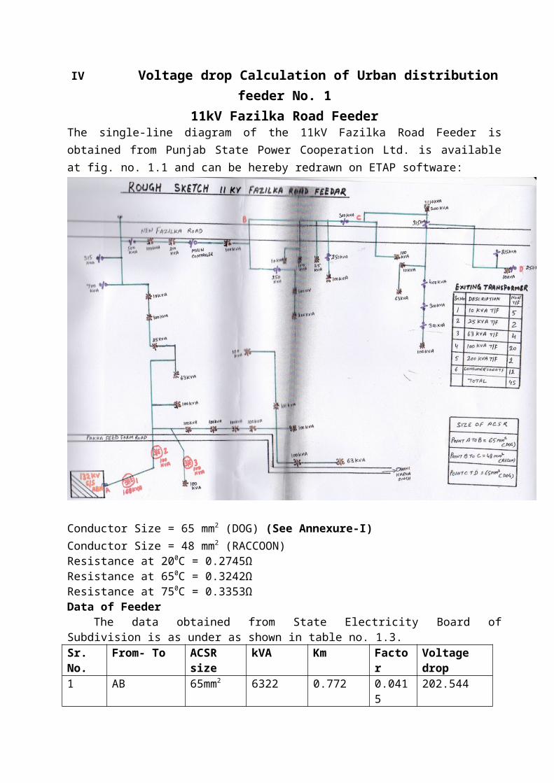
IV Voltage drop Calculation of Urban distributionfeeder No. 1

11kV Fazilka Road FeederThe single-line diagram of the 11kV Fazilka Road Feeder isobtained from Punjab State Power Cooperation Ltd. is availableat fig. no. 1.1 and can be hereby redrawn on ETAP software:

Conductor Size = 65 mm2 (DOG) (See Annexure-I)Conductor Size = 48 mm2 (RACCOON)Resistance at 200C = 0.2745Ω Resistance at 650C = 0.3242ΩResistance at 750C = 0.3353ΩData of Feeder

The data obtained from State Electricity Board ofSubdivision is as under as shown in table no. 1.3.Sr.No.

From- To ACSRsize

kVA Km Factor

Voltagedrop

1 AB 65mm2 6322 0.772 0.0415

202.544

2. BC 65mm2 5359 0.160 0.0415

35.584

3. CD 65mm2 5259 0.470 0.0415

102.577

4. DE 65mm2 5196 0.464 0.0415

100.054

5. E’E1 65mm2 5171 0.240 0.0415

51.503

6. E1E2 65mm2 5071 0.798 0.0415

167.936

7. E2F 65mm2 5061 0.542 0.0415

113.837

8. FG 65mm2 4361 0.240 0.0415

43.436

9. GH 65mm2 4046 0.146 0.0415

24.515

10. HI 65mm2 3546 0.134 0.0415

19.719

11. IJ 65mm2 3446 0.145 0.0415

20.736

12. JK 65mm2 3246 0.052 0.0415

7.005

13. KL 48mm2 2533 0.740 0.0499

93.534

14. LM 48mm2 2423 0.100 0.0499

12.091

15. MN 48mm2 2398 0.026 0.0499

3.111

16. NO 48mm2 2048 0.140 0.0499

14.307

17. OP 65mm2 1948 0.654 0.0415

52.871

18. PQ 65mm2 1738 0.045 0.0415

3.246

19. QR 65mm2 1423 0.100 0.0415

5.905

20. RS 65mm2 1173 0.315 0.0415

15.334

21. ST 65mm2 250 0.045 0.0415

0.467

Total Voltage drop 1090.312

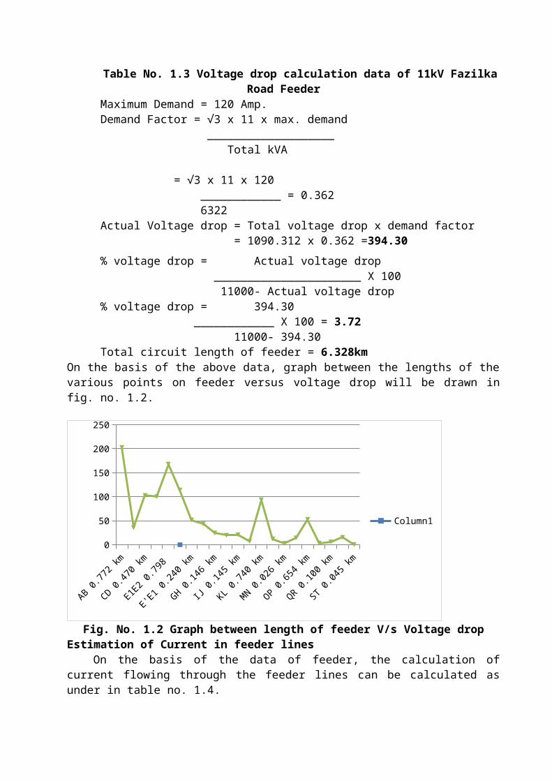
Table No. 1.3 Voltage drop calculation data of 11kV FazilkaRoad Feeder

Maximum Demand = 120 Amp. Demand Factor = √3 x 11 x max. demand

___________________ Total kVA

= √3 x 11 x 120 ____________ = 0.362

6322Actual Voltage drop = Total voltage drop x demand factor

= 1090.312 x 0.362 =394.30% voltage drop = Actual voltage drop

______________________ X 100 11000- Actual voltage drop

% voltage drop = 394.30 ____________ X 100 = 3.72

11000- 394.30 Total circuit length of feeder = 6.328km

On the basis of the above data, graph between the lengths of thevarious points on feeder versus voltage drop will be drawn infig. no. 1.2.

0

50

100

150

200

250

Column1

Fig. No. 1.2 Graph between length of feeder V/s Voltage dropEstimation of Current in feeder lines

On the basis of the data of feeder, the calculation ofcurrent flowing through the feeder lines can be calculated asunder in table no. 1.4.

Section Length inkm

Voltage Drop(Volts)

kVA Currentin

feederlines

AB 0.772 202.544 6322 331.82BC 0.160 35.584 5359 281.27CD 0.470 102.577 5259 276.03DE 0.464 100.054 5196 272.72

E’E1 0.240 51.503 5171 271.41E1E2 0.798 167.936 5071 266.16E2F 0.542 113.837 5061 265.63FG 0.240 43.436 4361 228.89GH 0.146 24.515 4046 212.36HI 0.134 19.719 3546 186.12IJ 0.145 20.736 3446 180.87JK 0.052 7.005 3246 170.37KL 0.740 93.534 2533 132.95LM 0.100 12.091 2423 127.17MN 0.026 3.111 2398 125.86NO 0.140 14.307 2048 107.49OP 0.654 52.871 1948 102.24PQ 0.045 3.246 1738 91.22QR 0.100 5.905 1423 74.69RS 0.315 15.334 1173 61.57ST 0.045 0.467 250 13.12

Total 6.328 km 1090.312Table No. 1.4 Estimation of current in feeder line

From the above calculations, it is assumed that the currentestimated on feeder line as reference current value at powerfactor of 0.88 (lagging).

Estimation of Current at different power factor:On the basis of the current estimation at reference power

factor of 0.88 (lagging), estimation of currents at other powerfactors, say 0.65 (lag) and unity power factor is also herebycalculated and is as under in table no. 1.5 on the basis ofrequired expression.

Current, I α 1Cos Φ

Section

Current at0.65 powerfactor

Current at 0.88power factor(reference)

Current atunity powerfactor

AB 245.09 331.82 377.07BC 208.20 281.27 319.63CD 203.89 276.03 313.67DE 201.44 272.72 309.91E’E1 200.47 271.41 308.42E1E2 196.60 266.16 302.45E2F 196.20 265.63 301.85FG 169.07 228.89 260.10GH 156.86 212.36 241.32HI 137.47 186.12 211.5IJ 133.60 180.87 205.53JK 125.84 170.37 193.60KL 98.20 132.95 151.08LM 93.93 127.17 144.51MN 92.96 125.86 143.02NO 79.39 107.49 122.15OP 75.52 102.24 116.18PQ 67.38 91.22 103.66QR 55.17 74.69 84.87RS 45.48 61.57 69.96ST 9.69 13.12 14.91

Table No. 1.5 Calculation of currents in feeder at various powerfactors

V CALCULATION OF VOLTAGE DROP AT VARIOUS POWER FACTORS &TEMPERATURE

Now voltage drop can be estimated at various power factors andalso at various temperatures of conductors.At power factor 0.88 (reference) and at various temperature Resistance at 200C = 0.2745Ω Resistance at 650C = 0.3242ΩResistance at 750C = 0.3353ΩOn the basis of the above parameters, the voltage dropcalculations had been estimated in table no. 1.6 at varioustemperatures i.e. 200C, 650C and at 750C Section Current at

0.88pf.Voltage drop

at 200C(reference)

Voltage dropat 650C

Voltage dropat 750C

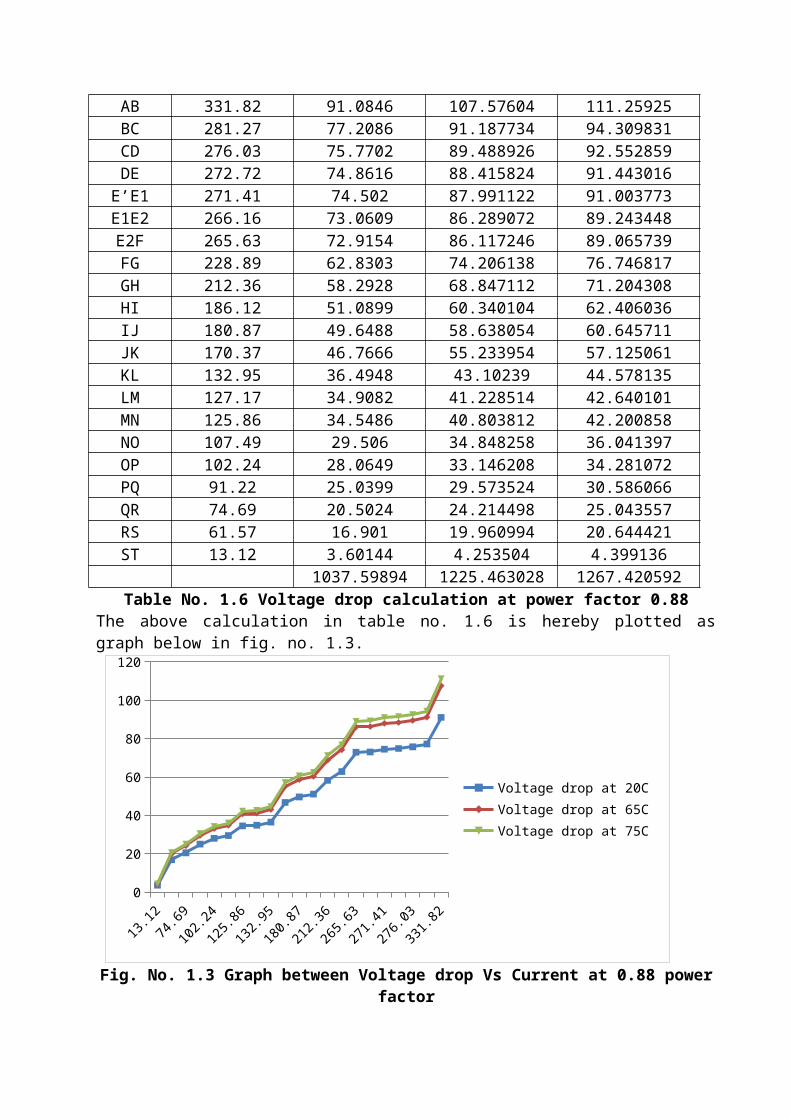
AB 331.82 91.0846 107.57604 111.25925BC 281.27 77.2086 91.187734 94.309831CD 276.03 75.7702 89.488926 92.552859DE 272.72 74.8616 88.415824 91.443016E’E1 271.41 74.502 87.991122 91.003773E1E2 266.16 73.0609 86.289072 89.243448E2F 265.63 72.9154 86.117246 89.065739FG 228.89 62.8303 74.206138 76.746817GH 212.36 58.2928 68.847112 71.204308HI 186.12 51.0899 60.340104 62.406036IJ 180.87 49.6488 58.638054 60.645711JK 170.37 46.7666 55.233954 57.125061KL 132.95 36.4948 43.10239 44.578135LM 127.17 34.9082 41.228514 42.640101MN 125.86 34.5486 40.803812 42.200858NO 107.49 29.506 34.848258 36.041397OP 102.24 28.0649 33.146208 34.281072PQ 91.22 25.0399 29.573524 30.586066QR 74.69 20.5024 24.214498 25.043557RS 61.57 16.901 19.960994 20.644421ST 13.12 3.60144 4.253504 4.399136

1037.59894 1225.463028 1267.420592Table No. 1.6 Voltage drop calculation at power factor 0.88

The above calculation in table no. 1.6 is hereby plotted asgraph below in fig. no. 1.3.

0

20

40

60

80

100

120

Voltage drop at 20C Voltage drop at 65CVoltage drop at 75C

Fig. No. 1.3 Graph between Voltage drop Vs Current at 0.88 powerfactor

At power factor 0.65 (lagging) and at various temperature Resistance at 200C = 0.2745Ω Resistance at 650C = 0.3242ΩResistance at 750C = 0.3353ΩOn the basis of the above parameters, the voltage dropcalculations had been estimated in table no. 1.7 at varioustemperatures i.e. 200C, 650C and at 750C Section Current at

0.65pf.(lag)

Voltage dropat 200C

(reference)

Voltage dropat 650C

Voltage dropat 750C


766.52761 905.31229 936.308485Table No. 1.7 Voltage drop calculation at power factor 0.65

(lag)The above calculation in table no. 1.7 is hereby plotted asgraph below in fig. no. 1.4.

0102030405060708090


Fig. No. 1.4 Graph between Voltage drop Vs Current at 0.65 (lag)power factor

At power factor Unity and at various temperatures Resistance at 200C = 0.2745Ω Resistance at 650C = 0.3242ΩResistance at 750C = 0.3353ΩOn the basis of the above parameters, the voltage dropcalculations had been estimated in table no. 1.8 at varioustemperatures i.e. 200C, 650C and at 750C Section Current at

Unity pf. Voltage drop

at 200C(reference)

Voltage dropat 650C

Voltage dropat 750C

AB 377.07 67.2772 79.458178 82.178677BC 319.63 57.1509 67.49844 69.80946CD 313.67 55.9678 66.101138 68.364317DE 309.91 55.2953 65.306848 67.542832E’E1 308.42 55.029 64.992374 67.217591E1E2 302.45 53.9667 63.73772 65.91998E2F 301.85 53.8569 63.60804 65.78586FG 260.10 46.4097 54.812494 56.689171GH 241.32 43.0581 50.854012 52.595158HI 211.5 37.7355 44.567774 46.093691IJ 205.53 36.6732 43.31312 44.79608JK 193.60 34.5431 40.797328 42.194152KL 151.08 26.9559 31.83644 32.92646LM 144.51 25.7838 30.452106 31.494729MN 143.02 25.5175 30.137632 31.169488

NO 122.15 21.7926 25.738238 26.619467OP 116.18 20.7302 24.483584 25.321856PQ 103.66 18.4958 21.844596 22.592514QR 84.87 15.1442 17.886114 18.498501RS 69.96 12.4843 14.744616 15.249444ST 14.91 2.65991 3.141498 3.249057

766.52761 905.31229 936.308485Table No. 1.8 Voltage drop calculation at Unity power factor

The above calculation in table no. 1.8 is hereby plotted asgraph below in fig. no. 1.5.

0

10

20

30

40

50

60

70

80

90


Fig. No. 1.5 Graph between Voltage drop Vs Current at Unitypower factor

VI ALTERATION OF ACSR CONDUCTOR SIZEAlteration of ACSR conductor means the size of conductor

used for obtaining voltage profile in the distribution feedercan be modified, so that voltage will be reached at the endconsumer will be within the limits as per desired norms.Alteration of conductor with specific size

The size of conductor used in the 11kV feeder, which is 65mm2

or 48mm2, can be modified with 80mm2 (LEOPARD).Existing Conductor Size of feeder = 65mm2 (DOG) Proposed Conductor Size of feeder = 80mm2 (LEOPARD)Resistance at 200C of proposed conductor = 0.2193Ω Resistance at 650C of proposed conductor = 0.2590ΩResistance at 750C of proposed conductor = 0.2679Ω

Thus, proposed voltage drops can be estimated at various powerfactors and also at various temperatures of conductors.At power factor 0.88 (reference) and at various temperature Resistance at 200C of proposed conductor = 0.2193Ω Resistance at 650C of proposed conductor = 0.2590ΩResistance at 750C of proposed conductor = 0.2679ΩOn the basis of the above parameters, the proposed voltage dropcalculations had been estimated in table no. 1.9 at varioustemperatures i.e. 200C, 650C and at 750C Section Current at

0.88pf.Voltage drop

at 200C(reference)

Voltage dropat 650C

Voltage dropat 750C


828.94523 979.00964 1334.9666Table No. 1.9 Proposed Voltage drop calculation at power factor

0.88The above calculation in table no. 1.9 is hereby plotted asgraph below in fig. no. 1.6.

0102030405060708090

100


Fig. No. 1.6 Graph between proposed Voltage drop Vs Current at0.88 power factor

At power factor 0.65 (lagging) and at various temperature Resistance at 200C of proposed conductor = 0.2193Ω Resistance at 650C of proposed conductor = 0.2590ΩResistance at 750C of proposed conductor = 0.2679ΩOn the basis of the above parameters, the voltage dropcalculations had been estimated in table no. 1.10 at varioustemperatures i.e. 200C, 650C and at 750C Section Current at

0.65pf.(lag)

Voltage dropat 200C

(reference)

Voltage dropat 650C

Voltage dropat 750C

AB 245.09 53.748237 63.47831 65.659611BC 208.20 45.65826 53.9238 55.77678CD 203.89 44.713077 52.80751 54.622131DE 201.44 44.175792 52.17296 53.965776E’E1 200.47 43.963071 51.92173 53.705913E1E2 196.60 43.11438 50.9194 52.66914E2F 196.20 43.02666 50.8158 52.56198FG 169.07 37.077051 43.78913 45.293853GH 156.86 34.399398 40.62674 42.022794HI 137.47 30.147171 35.60473 36.828213IJ 133.60 29.29848 34.6024 35.79144JK 125.84 27.596712 32.59256 33.712536KL 98.20 21.53526 25.4338 26.30778LM 93.93 20.598849 24.32787 25.163847

MN 92.96 20.386128 24.07664 24.903984NO 79.39 17.410227 20.56201 21.268581OP 75.52 16.561536 19.55968 20.231808PQ 67.38 14.776434 17.45142 18.051102QR 55.17 12.098781 14.28903 14.780043RS 45.48 9.973764 11.77932 12.184092ST 9.69 2.125017 2.50971 2.595951

612.38429 723.24455 748.09736Table No. 1.10 Proposed Voltage drop calculation at power factor

0.65 (lag)The above calculation in table no. 1.10 is hereby plotted asgraph below in fig. no. 1.7.

0

10

20

30

40

50

60

70


Fig. No. 1.7 Graph between proposed Voltage drop Vs Current at0.65 (lag) power factor

At power factor Unity and at various temperatures Resistance at 200C of proposed conductor = 0.2193Ω Resistance at 650C of proposed conductor = 0.2590ΩResistance at 750C of proposed conductor = 0.2679ΩOn the basis of the above parameters, the voltage dropcalculations had been estimated in table no. 1.11 at varioustemperatures i.e. 200C, 650C and at 750C Section Current at

Unity pf. Voltage drop

at 200C(reference)

Voltage dropat 650C

Voltage dropat 750C

AB 377.07 82.691451 97.66113 101.01705BC 319.63 70.094859 82.78417 85.628877CD 313.67 68.787831 81.24053 84.032193

DE 309.91 67.963263 80.26669 83.024889E’E1 308.42 67.636506 79.88078 82.625718E1E2 302.45 66.327285 78.33455 81.026355E2F 301.85 66.195705 78.17915 80.865615FG 260.10 57.03993 67.3659 69.68079GH 241.32 52.921476 62.50188 64.649628HI 211.5 46.38195 54.7785 56.66085IJ 205.53 45.072729 53.23227 55.061487JK 193.60 42.45648 50.1424 51.86544KL 151.08 33.131844 39.12972 40.474332LM 144.51 31.691043 37.42809 38.714229MN 143.02 31.364286 37.04218 38.315058NO 122.15 26.787495 31.63685 32.723985OP 116.18 25.478274 30.09062 31.124622PQ 103.66 22.732638 26.84794 27.770514QR 84.87 18.611991 21.98133 22.736673RS 69.96 15.342228 18.11964 18.742284ST 14.91 3.269763 3.86169 3.994389

941.97903 1112.506 1150.735Table No. 1.11 Proposed Voltage drop calculation at Unity power

factor The above calculation in table no. 1.11 is hereby plotted asgraph below in fig. no. 1.8.

020406080

100120


Fig. No. 1.8 Graph between proposed Voltage drop Vs Current atUnity power factor

VII CONCLUSION

Hence, it has been observed that the existing feeder is to beoperated on 0.88power factor at a temperature range of conductorat 200C, however it is come to notice while analysing that theconductor size can be augmentated with 65mm2 (DOG) and 48mm2

(RACCOON) to the use of 80mm2 (LEOPARD) and 50mm2 (OTTER) forreduction of voltage drop in feeder, due to its better currentcarrying capacity of 375A in comparison of 324A of 65mm2

conductor and same linear coefficient of temperature rise andmodulus of elasticity, as observed from the diagram obtainedafter analysis. But the weight of 80mm2 conductor is 27.9mm2 increased, which canbe supported by the existing structures installed in the feederarea. Location, proper placement and sizing of the capacitor banks forimproving the power factors and harmonics in the 11 kV urbandistribution feeders of the Subdivision can be investigated forimprovement in system performance. Effects of High VoltageDistribution systems (HVDS) on the 11kV distribution feederswill be considered for better solutions. Effects of under sizingof the conductors was checked and recommendation for propersizing of the conductors is hereby recommended for operation.Estimation of Hot spots will be checked and thus the performancewill be enhanced and estimation of poor jointing andterminations will be another methodology for proper faultmaintenance to be carried out.

VIII REFERENCES[1] Soloman Nunoo, Joesph C. Attachie and Franklin N. Duah, “ An

Investigation into the Causes and Effects of Voltage dropson 11KV Feeder”, Canadian Journal of Electrical andElectronics Engineering, Vol. 3, January, 2012.

[2] Vujosevic, L. Spahic E. and Rakocevic D., “One Method forthe Estimation of voltage drop in Distribution System”,http://www.docstoc.com/document/ education, March, 2011.

[3] Konstantin S. Turitsyn, “Statistics of voltage drop inradial distribution circuits: a dynamic programmingapproach”, arXiv,:1006.0158v, June, 2010.

[4] C.G. Carter-Brown and C.T. Gaunt, “Model for theapportionment of the total voltage drop in Combined Mediumand Low Voltage Distribution Feeders”, Journal of SouthAfrican Institute of Electrical Engineers, Vol. 97(1),March, 2006.

http://www.docstoc.com/document/%20education

[5] C.G. Carter-Brown, “Voltage drop apportionment in Eskom’sdistribution networks”, Masters dissertation, University ofCape Town South Africa, pp. 28-33, 50,52,55,60, 2002.

[6] C.G. Carter-Brown, “Optimal voltage regulation limits andvoltage drop apportionment in distribution systems”, 11th

Southern African Universities Power Engineering Conference(SAUPEC, 2002) pp. 318-322, Jan/Feb., 2002.

[7] S.A. Qureshi and F. Mahmood, “Evaluation by implementationof Distribution System Planning for Energy Loss Reduction”,Pal. J. Engg. & Appl. Sci., Vol. 4, pp. 43-45, January,2009.

[8] M. Amin., M.Sc. Thesis, Electrical Engineering Department,UET, Lahore, Pakistan, 2006.

[9] D. Beg. and J. R. Armstrong, “Estimation of Technical Lossesfor Distribution system Planning”, IEEE Power EngineeringJournal, Vol. 3, pp. 337-343, 1989.

[10] Sarang Pande and Prof. J. G. Ghodekar, “Computation ofTechnical Power Loss of Feeders and Transformers inDistribution System using Load Factor and Load Loss Factor”,International Journal of Multidisciplinary Sciences andEngineering, Vol 3. No. 6, June, 2012.

Annexure-ITable: Aluminium Conductor Steel Reinforced [Based on IS: 398(1961)]

Conductor Electricalproperties

Stranding andWire diameter

Mechanical Properties

Codename

Nominal cu area mm2

Equivalent

area ofAl mm2

Calculated

resist.At 200CΩ/km

Approx.

current

carrying

capacity400C

Al.No.

Al.Dia.

SteelNo.

Steeldia.

Conductor dia.

mm

Conductor area

mm2

Totalwt.

Wt.ofAl.

Wt.ofsteel

Approx. Utl.Strength

Linearcoeff.per0C x10-6

Modulus ofelasticitykg/cm2 x106

1 2 3 4 5 6 7 8 9 10 11 12 13 14 15 16 17MOLE 6.5 10.47 2.71800 - 6 1.5

01 1.5

04.50 12.37 43 29 14 408 18.99 0.809

SQUIRREL 13 20.71 1.37400 115 6 2.11

1 2.11

6.33 24.48 85 58 27 771 18.99 0.809

GOPHER 16 25.91 1.09800 133 6 2.36

1 2.36

7.08 30.62 106 72 34 952 18.99 0.809

WEASEL 20 31.21 0.91160 150 6 2.59

1 2.59

7.77 36.88 128 87 41 1136 18.99 0.809

FERRET 25 41.87 0.67950 181 6 3.00

1 3.00

9.00 49.48 171 116 55 1503 18.99 0.809

RABBIT 30 52.21 0.544+0 208 6 3.35

1 3.35

10.05 61.71 214 145 69 1860 18.99 0.809

MINK 40 62.32 0.45650 234 6 3.66

1 3.66

10.98 73.65 255 172 82 2208 18.99 0.809

HORSE 42 71.58 0.39770 - 12 2.79

7 2.79

13.95 116.20 542 204 338 6108 15.30 1.070

BEAVER 45 74.07 0.38410 261 6 3.99

1 3.99

11.97 87.53 303 205 98 2613 18.99 0.809

RACCOON 48 77.83 0.3646 270 6 4.09

1 4.09

12.27 91.97 218 215 103 2746 18.99 0.809

OTTER 50 82.85 0.34340 281 6 4.2 1 4.2 12.66 97.91 339 230 109 2923 18.99 0.809

2 2CAT 55 94.21 0.30200 305 6 4.5

01 4.5

013.50 111.30 385 261 125 3324 18.99 0.809

DOG 65 103.60 0.27450 324 6 4.72

7 1.57

14.16 118.50 394 288 109 2399 19.53 0.735

LEOPARD 80 129.70 0.21930 375 6 5.28

7 1.76

15.84 148.40 493 360 133 4137 19.53 0.735

COYOTE 80 128.50 0.22140 375 26 2.51

7 1.90

15.86 151.60 521 365 156 4638 18.99 0.773

TIGER 80 128.10 0.22210 382 30 2.36

7 2.36

16.52 161.80 604 363 241 5758 17.73 0.787

WOLF 95 154.30 0.18440 430 30 2.59

7 2.59

1.13 195.00 727 436 291 6880 17.73 0.787

LYNX 110 179.00 0.15890 475 30 2.79

7 2.79

19.53 226.20 844 506 338 7950 17.73 0.787

PANTHER 130 207.00 0.13750 520 30 3.00

7 3.00

21.00 261.60 976 586 390 9127 17.73 0.787

LION 140 232.30 0.12230 555 30 3.18

7 3.18

22.26 293.90 1097 659 438 10210 17.73 0.787

BEAR 160 258.10 0.11020 292 30 3.35

7 3.35

23.45 326.10 .1219

734 485 11310 17.73 0.787

GOAT 185 316.50 0.08989 680 30 3.71

7 3.71

25.97 400.00 1492 896 596 13780 17.73 0.787

SHEEP 225 366.10 0.07771 745 30 3.99

7 3.99

27.93 462.60 1726 1036

690 15910 17.73 0.787

KUNDAH 250 394.40 0.07434 - 42 3.50

7 1.94

26.82 424.80 1282 1120

162 9002 21.42 0.646

DEER 260 419.30 0.06786 806 30 4.27

7 4.27

29.89 529.40 1977 1188

789 18230 17.73 0.787

ZEBRA 260 418.60 0.06800 795 54 3.18

7 3.18

28.62 484.50 1623 1185

438 13316 19.35 0.686

ELK 300 465.70 0.06110 860 30 4.50

7 4.50

31.50 588.40 2196 1320

876 20240 17.73 0.787

CAMEL 300 464.50 0.06125 - 54 3.35

7 3.35

30.15 537.70 1804 1318

486 14750 19.36 0.686

MOOSE 325 515.70 0.05517 900 54 3.53

7 3.53

3177 597.11 2002 1463

539 16250 19.53 0.686

SPARROW 20 33.16 0.85780 - 6 2.67

1 2.67

8.01 39.22 135 92 43 1208 18.99 0.809

FOX 22 36.21 0.78570 165 6 2.79

1 2.79

9.37 42.92 149 101 48 1313 18.99 0.809

Documents

vDESIGN OF URBAN DISTRIBUTION FEEDERS FOR VOLTAGE PROFILE IMPROVEMENT & DISTRIBUTION LOSSES REDUCTION