Embed Size (px)
Citation preview
1
pSudan University of Science and Technology College of Postgraduate Studies
Department of Plastics Engineering
Viscosity Measurement by using Melt flow Index for Thermoplastic polymers
ك لبالس مير از معامل انصهار البو دام ست ه لزو اس ا احلراريق
A thesis Submitted in Partial Fulfillment of the Requirements for the degree of Masters of Science (in Plastic Engineering)
By: Maysaa Elrasheed Rahamtalla Mohamed Supervisor: Dr. Mohamed Deen Hussein Mohamed
April 2014

I
Dedication
Dedicated
To our parents with all our love
To our sisters
, our brothers
& our teachers who help us…
To our colleagues….

II
ACKNOWLEDGEMENT
I would like to express my gratitude to Dr. Mohamed
Deen Hussien, my advisor, for his constant guidance
and constructive criticism which have helped me to
accomplish this work and improve my technical
abilities.
This is an opportunity to express my sincere thanks also
to the each teacher in the Department of Plastic
Engineering for the help and advice I received over the
years and to all my friends for their continuous support
here at Sudan University and Science technology –
Engineering Collage. I would also like to especially
thank my colleagues Arman Mohammed Abdalla
Ahmed and Muhab Slah Shalby to help me during every
stage of this work.
Finally, I would like to thank my dear mother for their
priceless support, love and never failing faith in me.
III
ABSTRACT In plastics manufacturing, the melt flow index (MFI) is used as a routine
indicator of rheological behavior when more expensive and laborious
determinations of well-defined material functions are impractical. The MFI is the
mass flow rate in a pressure driven flow through a standardized abrupt cylindrical
contraction into a short tube performed under a standardized combination of
pressure drop and temperature. In this research, we used Polyethylene low density
grade of extrusion and poly propylene grade of injection to explore the connections
between rheological properties and melt index.
We explore the role of shear by modeling the flow through the melt indexer using
the different applied loads from 1.2 to 5 kg at different temperature to the same
material to give us different value of MFI, and then calculate the mass flow rate,
volume flow rate, pressure difference, viscosity, maximum shear stress and
maximum shear rate. It was found that the viscosity is affected by temperature,
changing the temperature change of the value of viscosity, and this change is
inversely.
We present our results in different charts designed to help plastics engineers
specify the MFI of a plastic for an industrial manufacturing process of known
material functions.

IV
المســتخلص
یستخدم معامل انسیاب المصھور في عملیات تصنیع البالستیك كمؤشر روتیني للسلوك
دید ھذا السلوك باإلختبارات المعملیھ االخرى مكلف وشاق ویحتاج الى حالریولوجي حیث ت
معامل انسیاب المصھور ھو معدل انسیاب الكتلھ . زمن طویل وبعبارة اخرى غیر عملي
. لمعرضھ لضغط محدد من خالل قالب قیاسي ذو مجرى اسطواني وعند درجة حرارة محددها
في ھذا البحث یستخدم البولي ایثلین منخفض الكثافھ والبولي بروبلین ألیجاد العالقات ما بین
بأستخدام جھاز قیاس ،ألیجاد تأثیر القص. الخواص الریولوجیھ ومعامل انسیاب المصھور
كیلوجرام عند درجات حرارة 5الى 1.2احمال مختلفھ من بتطبیق مصھورمعامل انسیاب ال
مختلفة لنفس الماده للحصول على قراءات مختلفة لمعامل انسیاب المصھور ومن ثم نحسب
والقیم القصوى ألجھاد , اللزوجة, الضغط, نسیاب الحجمياالمعدل ,ھ یاب الكتلمعدل انس
الحرارة درجات وتغییر ,وجد ان اللزوجة تتأثر بدرجة الحرارة .نفعال القصإالقص ومعدل
,یغیر من قیمة اللزوجة .وھذا التغییر یكون عكسیاناعیھ ھ الص د العملی تیك لتحدی ي البالس اعدة مھندس ات لمس ي مخطط ائج ف ت النت عرض
. لخصائص المادة وفقـا
V
TABLE OF CONTENTS
I االیــة
Dedication ……………………………………………………………………… II
Acknowledgement ……………………………………………………………... III
Abstract in English ……………………………………………………………. IV
Abstract in Arabic ……………………………………………………………... V
Table of Contents ……………………………………………………………… VI
List of Table …………………………………………………………………..... VII
List of Figures and Plates……………………………………………………… VIII
List of abbreviation…………………………………………………………… IX
1. CHAPTER ONE INTRODUCATION ………………………………. 1
1.1. Introduction …………………………………………………………. ……. 1
1.2. Background ………………………………………………………………. 3
1.2.1 Polymers…………………………………………………………….. 3
1.3. Objectives of present study …………………………………………………… 8
2. CHAPTER TWO LITERTURE REVIEW …………………..... 10
2.1. Introduction ………………………………………………………………… 10
2.2. Rheology ………………………………………............................................ 10
2.2.1 Viscosity ……………………………………….......................... 10
2.3. Other Relationships for Shear Viscosity Function …………………………. 15
2.3.1 Viscosity-Temperature Relationships ………………………….. 15
2.3.2 viscosity-Pressure Relationship …………………………........... 17
2.3.3 Viscosity-Molecular Weight Relationship ………...................... 17
2.3.4Shear-Rate-Dependent Viscosity Laws…………………………. 17
VI
2.4 Rheometers for polymer melt characterization……………………………... 21
2.5. Processing Polymers …………………………………………………….. 22
2.5.1 Extrusion ……………………………………………………….. 22
2.5.2 Injection molding ………………………………………………. 24
2.6. Review of literature ………………………………………………………… 26
3. CHAPTER THREE MTERIAL AND METHOD……………………. 28
3.1. Introduction ………………………………………………………………… 28
3.2 .Method……………………………………………………………………… 29
3.3. Techniques used to calculate mass flowG, volume flowV, viscosityη, maximum
shear stress τ and maximum shear rateγ ………………………………..
31
3.3.1 Basics, viscosity law of Newton…………………………………... 31
3.3.2 Flow in capillary…………………………………………………... 34
3.4 Evaluation of standard test………………………………………………….. 37
3.4.1Evaluation of MFI test……………………………………………….. 38
4. CHAPTER FOUR RESULT AND DISSCUSIN………………………. 41
4.1. Introduction………………………………………………………………… 41
4.1.1Low density Polyethylene (LDPE) …………………………………… 41
4.1.2 Polypropylene (PP)…………………………………………………… 47
5. CHAPTER FIVE CONCLUSIONS AND RECOMMENDATIONS 52
REFERENCES…………………………………………………………………. 54
APPENDICES (A) Low density polyethylene……………………………….. 56
APPENDICES (B) Polypropylene…………………………………………... 61
VII
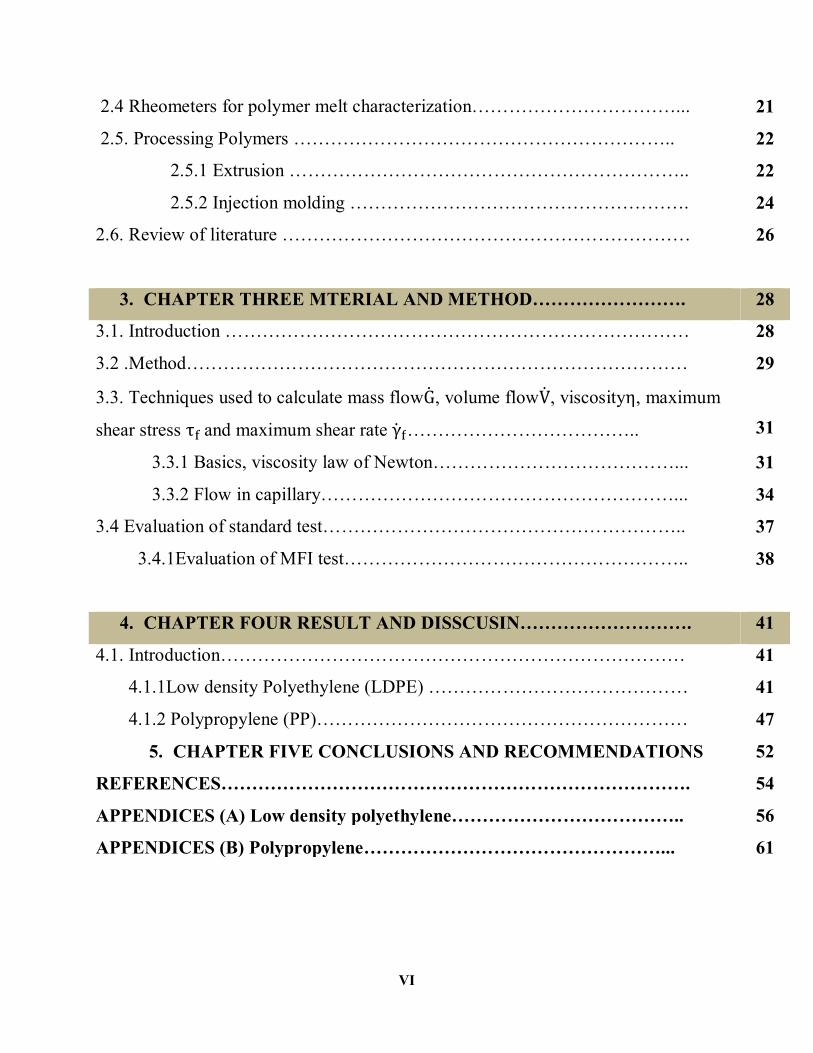
LIST OF FLOW CHARTS & TABLES
Flow chart Page
1.1. polymer Classification Based on Chemical
6
1.2. polymer Classification Based on Structure
7
2.1. Rheometers for flow of Thermoplastic Melts
21
2.2.
Table
Shaping Operations
23
Page 3.1. The basic characteristics of the used material
28
VIII
LIST OF FIGURES AND PLATES
Figure Page
2.1. Simple shear flow. 11
2.2. Velocity, shear rate and shear stress profiles for flow between two flat plates.
12
2.3. Newtonian fluid) relationship between shear rate, shear stress and viscosity.
13
2.4. Qualitative flow curves for different types of non-Newtonian fluids 14
2.5. (Thixotropy and Rheopexy) relationship between shear rates, shear stress
15
2.6. Sketch of an extrusion line.
24
2.7. .Major parts of a typical injection-molding machine 25
3.1. Typical apparatus for determining melt flow rate (showing one of the possible methods of retaining the die and one type of piston)
29
3.2. Deformation of solid body and fluid layer 31
3.3. Velocity distributions in fluid layer 33
3.4. Pressure distribution along the capillary 35
3.5. Distribution of τ shear stress and flow velocity in the cross section of the capillary.
36
4.1. Viscosity V.S shear rate curve for (LDPE at 2100C, 1900C & 1700C). 42
4.2. Relation between Shear Stress and Shear Rate for (LDPE at 2100C ,1900C & 1700C).
42
4.3. Experimental viscosity with power law model
43
IX
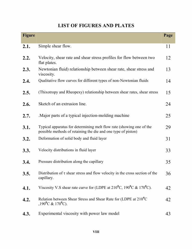
4.4. Relation between Melt flow index MFI (g/10min) and load (kg)
44
4.5. Logarithm of zero shear rate viscosity VS. 1000 푇⁄
45
4.6. Experimental viscosity with carreau model.
46
4.7. Viscosity V.S shear rate curve for (PP at 1900C, 2100C & 2300C). 47
4.8. . Relation between Shear Stress and Shear Rate for (PP at 1900C ,2100C & 2300C).
48
4.9. Experimental viscosity for PP with power law model 49
4.10. Relation between Melt flow index MFI (g/10min) and load (kg) for pp.
50
4.11. Experimental viscosity for PP with carreau model 51
X
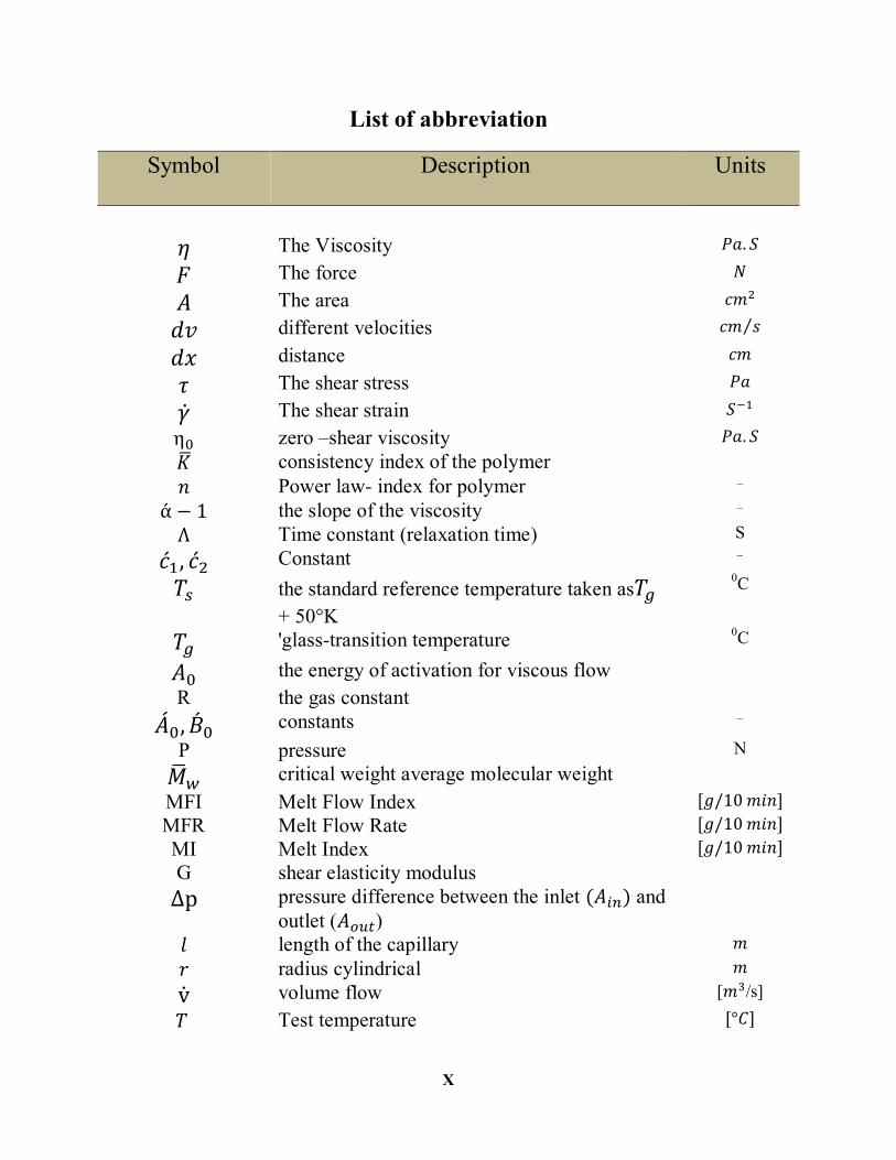
List of abbreviation
Symbol Description Units
휂 The Viscosity 푃푎. 푆
퐹 The force 푁
퐴 The area 푐푚
푑푣 different velocities 푐푚 푠⁄
푑푥 distance 푐푚
휏 The shear stress 푃푎
훾 The shear strain 푆
η zero –shear viscosity 푃푎. 푆 퐾 consistency index of the polymer 푛 Power law- index for polymer _
α − 1 the slope of the viscosity _ Λ Time constant (relaxation time) S
푐 , 푐 Constant _
푇 the standard reference temperature taken as푇 + 50°K
0C
푇 'glass-transition temperature 0C
퐴 the energy of activation for viscous flow
R the gas constant
퐴 ,퐵 constants _
P pressure N
푀 critical weight average molecular weight
MFI Melt Flow Index [푔/10푚푖푛] MFR Melt Flow Rate [푔/10푚푖푛] MI Melt Index [푔/10푚푖푛] G shear elasticity modulus
∆p pressure difference between the inlet (퐴 ) and outlet (퐴 )
푙 length of the capillary 푚 푟 radius cylindrical 푚
v volume flow [푚 /s]
푇 Test temperature [°퐶]
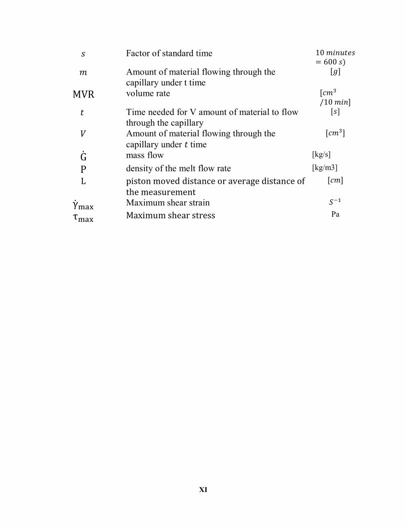
XI
푠 Factor of standard time 10푚푖푛푢푡푒푠= 600푠)
푚 Amount of material flowing through the capillary under t time
[푔]
MVR volume rate [푐푚/10푚푖푛]
푡 Time needed for V amount of material to flow through the capillary
[푠]
푉 Amount of material flowing through the capillary under 푡time
[푐푚 ]
G mass flow [kg/s]
Ρ density of the melt flow rate [kg/m3]
L pistonmoveddistanceoraveragedistanceofthemeasurement
[푐푚]
γ Maximum shear strain 푆
τ Maximumshearstress Pa
1
CHAPTER ONE
INTRODUCTION
1.1. Introduction:
Anyone beginning the process of learning to think Rheo-Logically must first ask
the question, "Why should I make a viscosity measurement?" The answer lies in
the experiences of thousands of people who have made such measurements,
showing that much useful behavioral and predictive information for various
products can be obtained, as well as knowledge of the effects of processing,
formulation changes, aging phenomena, etc.
A frequent reason for the measurement of rheological properties can be found in
the area of quality control, where raw materials must be consistent from batch to
batch. For this purpose, flow behavior is an indirect measure of product
consistency and quality.
Another reason for making flow behavior studies is that a direct assessment of
process ability can be obtained. For example, a high viscosity liquid requires more
power to pump than a low viscosity one. Knowing its rheological behavior,
therefore, it is useful when designing pumping and piping systems.
It has been suggested that rheology is the most sensitive method for material
characterization because flow behavior is responsive to properties such as
molecular weight and molecular weight distribution. Rheological measurements
are also useful in following the course of a chemical reaction. Such measurements
can be employed as a quality check during production or to monitor and/or control
a process. Rheological measurements allow the study of chemical, mechanical, and
thermal treatments, the effects of additives, or the course of a curing reaction. They
2
are also a way to predict and control a host of product properties, end use
performance and material behavior.
Viscosity is the most important flow property, and it is the resistance to shearing,
there are many different techniques for measuring viscosity. In capillary
viscometers like (Melt Flow Index Tester), the shear stress is determined from the
pressure applied by a piston. The shear rate is determined from the flow rate.
Significance and use the melt flow index:
1- This test method is particularly useful for quality control tests on
thermoplastics.
2- This test method serves to indicate the uniformity of the flow rate of
polymer as made by an individual process and, in this case, may be
indicative of uniformity of other properties. However, uniformity of flow
rate among various polymers as made by various processes does not, in the
absence of other tests, indicate uniformity of other properties.
3- The flow rate obtained with the extrusion plastometer is not a fundamental
polymer property. It is an empirically defined parameter critically influenced
by the physical properties and molecular structure of the polymer and the
conditions of measurement. The rheological characteristics of polymer melts
depend on a number of variables. Since the values of these variables
occurring in this test may differ substantially from those in large-scale
processes, test results may not correlate directly with processing behavior
[8].
3
1.2. BACKGROND
1.2.1 Polymers:
Polymers are a large class of materials consisting of many small molecules (called
monomers) that can be linked together to form long chains, thus they are known as
macromolecules. A typical polymer may include tens of thousands of monomers.
Because of their large size, polymers are classified as macromolecules [9].
Polymer Classification:
A. Plastics – Greek word plastikos (Thermoplastics, Thermosets)
The polymer chains can be free to slide past one another (thermoplastic) or they
can be connected to each other with cross links (thermoset). Thermoplastics
(including thermoplastic elastomers) can be reformed and recycled, while
thermosets (including cross linked elastomers) are not re workable.
1- Thermoplastics:
Polymers that flow when heated; thus, easily reshaped and recycled. This property
is due to presence of long chains with limited or no cross links. In a thermoplastic
material the very long chain-like molecules are held together by relatively weak
Vander Waals forces. When the material is heated the intermolecular forces are
weakened so that it becomes soft and flexible and eventually, at high temperatures,
it is a viscous melt (it flows). When the material is allowed to cool it solidifies
again.
For example: polyethylene (PE), polypropylene (PP), poly (vinyl chloride)
(PVC), polystyrene (PS), poly (ethylene terephthalate) (PET), nylon
(polyamide), & unvulcanized natural rubber (polyisoprene).
4
2- Thermosets:
Decompose when heated; thus, cannot be reformed or recycled. Presence of
extensive cross links between long chains induces decomposition upon heating and
renders thermosetting polymers brittle.
A thermosetting polymer is produced by a chemical reaction which has two
stages. The first stage results in the formation of long chain-like molecules similar
to those present in thermoplastics, but still capable of further reaction. The second
stage of the reaction (cross linking of chains) takes place during moulding, usually
under the application of heat and pressure. During the second stage, the long
molecular chains have been interlinked by strong covalent bonds so that the
material cannot be softened again by the application of heat. If excess heat is
applied to these materials they will char and degrade.
For example: epoxy, unsaturated polyesters, phenol-formaldehyde resins,
vulcanized rubber.
B. Elastomers:
The polymer chains in elastomers are above their glass transition at room
temperature, making them rubbery. Can undergo extensive elastic deformation.
Elastomeric polymer chains can be cross linked, or connected by covalent bonds.
Cross linking in elastomers is called vulcanization, and is achieved by irreversible
chemical reaction, usually requiring high temperatures.
UN vulcanized natural rubber (polyisoprene) is a thermoplastic and in hot weather
becomes soft and sticky and in cold weather hard and brittle. It is poorly resistant
to wear. Sulfur compounds are added to form chains that bond adjacent polymer
5
backbone chains and cross links them. The vulcanized rubber is a thermosetting
polymer.
Cross linking makes elastomers reversibly stretchable for small deformations.
When stretched, the polymer chains become elongated and ordered along the
deformation direction. This is entropically unfavorable. When no longer stretched,
the chains randomize again. The cross links guide the elastomer back to its original
shape.
For example: natural rubber (polyisoprene), polybutadiene (used in shoe soles and
golf balls), polyisobutylene (used in automobile tires), butyl rubber (pond
and landfill linings), styrene butadiene rubber – SBR (used in automobile
tires) and silicone.
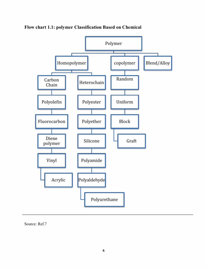
Polymer classification can be done in a number of different ways, as shown in flow
charts 1.1 – 1.2
6
Flow chart 1.1: polymer Classification Based on Chemical
Source: Ref.7
Polymer
Homopolymer
Carbon Chain
Polyolefin
Fluorocarbon
Diene polymer
Vinyl
Acrylic
Heterochain
Polyester
Polyether
Silicone
Polyamide
Polyaldehyde
Polyurethane
copolymer
Random
Uniform
Block
Graft
Blend/Alloy
7
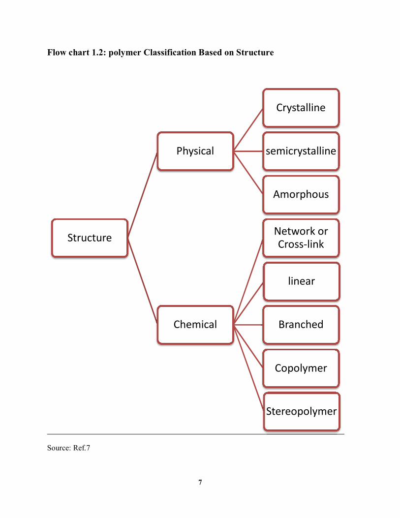
Flow chart 1.2: polymer Classification Based on Structure
Source: Ref.7
Structure
Physical
Crystalline
semicrystalline
Amorphous
Chemical
Network or Cross-link
linear
Branched
Copolymer
Stereopolymer
8
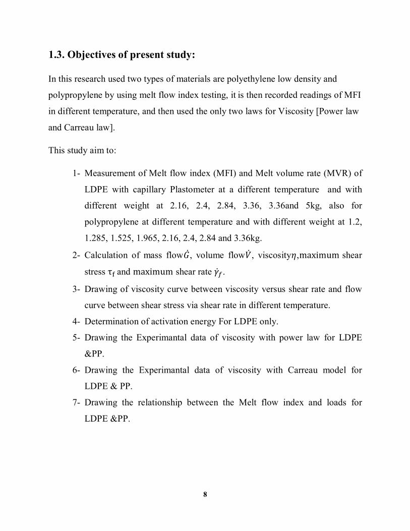
1.3. Objectives of present study:
In this research used two types of materials are polyethylene low density and
polypropylene by using melt flow index testing, it is then recorded readings of MFI
in different temperature, and then used the only two laws for Viscosity [Power law
and Carreau law].
This study aim to:
1- Measurement of Melt flow index (MFI) and Melt volume rate (MVR) of
LDPE with capillary Plastometer at a different temperature and with
different weight at 2.16, 2.4, 2.84, 3.36, 3.36and 5kg, also for
polypropylene at different temperature and with different weight at 1.2,
1.285, 1.525, 1.965, 2.16, 2.4, 2.84 and 3.36kg.
2- Calculation of mass flow퐺, volume flow푉, viscosity휂,maximum shear
stress τ and maximum shear rate훾 .
3- Drawing of viscosity curve between viscosity versus shear rate and flow
curve between shear stress via shear rate in different temperature.
4- Determination of activation energy For LDPE only.
5- Drawing the Experimantal data of viscosity with power law for LDPE
&PP.
6- Drawing the Experimantal data of viscosity with Carreau model for
LDPE & PP.
7- Drawing the relationship between the Melt flow index and loads for
LDPE &PP.
9
Thesis out lines:
This thesis is divided into five chapters
Chapter one gives relevant information on Classification of polymer.
Chapter two presents introduction of Reology including viscosity and types
of viscosity, Other Relationships for Shear Viscosity Function, Rheometers
for polymer melt characterization, polymer processing, a literature review
and objectives of present study.
Chapter three Review the way the device used with a description of its parts
and the method of operation of the device, Techniques used to calculate
mass flow G , volume flow V , viscosityη , maximum shear stress τ and
maximum shear rateγ , Evaluation of standard test
Chapter four present all of charts of low density polyethylene and
polypropylene.
Chapter five the conclusion and recommendations based on this study are
summarized in this chapter.
10
CHAPTER TWO
LITERTURE REVIEW
2.1. Introduction:
Numerous publications have been reported on the rheological characterization of
polymers. However, most of these publications pertain either to pure rheological
characterization, with emphasis on finding possible explanations for certain
observed polymer behaviors, or to the mathematical modeling of polymer behavior
during the processing. Very few attempts have been made to characterize the
rheological properties of resin, with the effect of rheology on resin process ability
as the ultimate objective. In this chapter, some of publications related to this work
are reviewed. But before displaying previous research, we explain some of the
concepts related to the polymers behavior.
2.2. Rheology:
Rheology is the science of deformation and flow of materials. The Society of
Rheology has a Greek motto "Panta Rei" translates as "All things flow." Actually,
all materials do flow, given sufficient time. What makes polymeric materials
interesting in this context is the fact that their time constants for flow are of the
same order of magnitude as their processing times for extrusion, injection molding
and blow molding [3]. In very short processing times, the polymer may behave as a
solid, while in long processing times the material may behave as a fluid. This dual
nature (fluid-solid) is referred to as viscoelastic behavior [3].
2.2.1 Viscosity:
Viscosity is the measure of the internal friction of a fluid. This friction becomes
apparent when a layer of fluid is made to move in relation to another layer. The
11
greater the friction, the greater the amount of force required to cause this
movement, which is called shear. Shearing occurs whenever the fluid is physically
moved or distributed, as in pouring, spreading, spraying, mixing, etc. Highly
viscous fluids, therefore, require more force to move than less viscous materials.
Viscosity is the most important flow property. It represents the resistance to flow.
Strictly speaking, it is the resistance to shearing, i.e., flow of imaginary slices of a
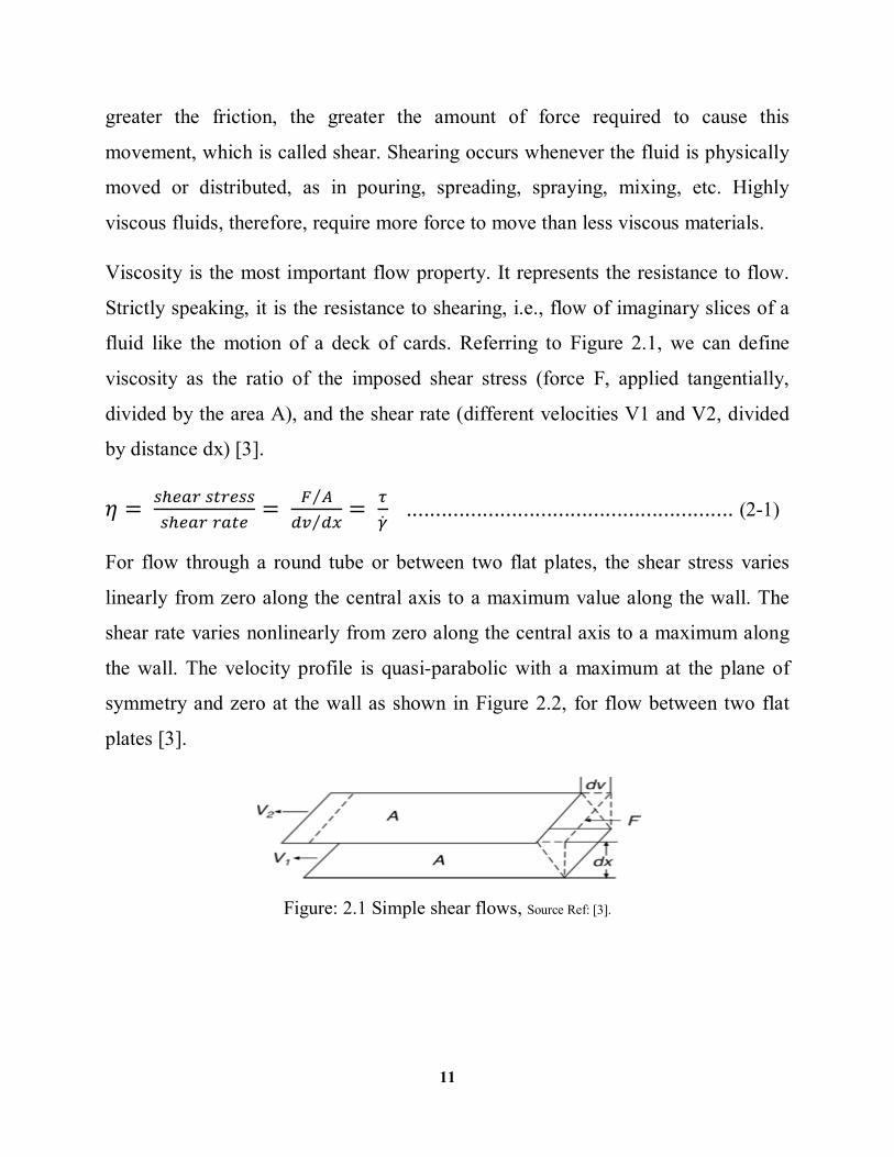
fluid like the motion of a deck of cards. Referring to Figure 2.1, we can define
viscosity as the ratio of the imposed shear stress (force F, applied tangentially,
divided by the area A), and the shear rate (different velocities V1 and V2, divided
by distance dx) [3].
휂 =
= ⁄⁄ =
........................................................ (2-1)
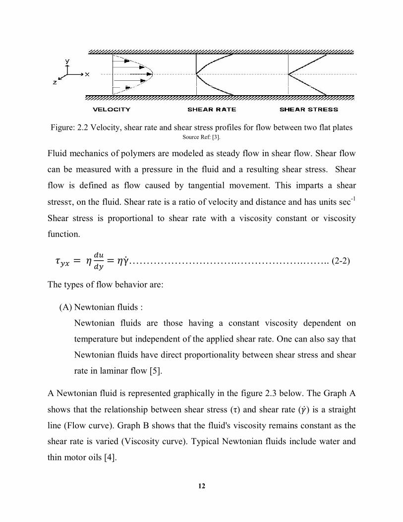
For flow through a round tube or between two flat plates, the shear stress varies
linearly from zero along the central axis to a maximum value along the wall. The
shear rate varies nonlinearly from zero along the central axis to a maximum along
the wall. The velocity profile is quasi-parabolic with a maximum at the plane of
symmetry and zero at the wall as shown in Figure 2.2, for flow between two flat
plates [3].
Figure: 2.1 Simple shear flows, Source Ref: [3].
12
Figure: 2.2 Velocity, shear rate and shear stress profiles for flow between two flat plates Source Ref: [3].
Fluid mechanics of polymers are modeled as steady flow in shear flow. Shear flow
can be measured with a pressure in the fluid and a resulting shear stress. Shear
flow is defined as flow caused by tangential movement. This imparts a shear
stress, on the fluid. Shear rate is a ratio of velocity and distance and has units sec-1
Shear stress is proportional to shear rate with a viscosity constant or viscosity
function.
휏 = 휂 = 휂γ………………………….……………….…….. (2-2)
The types of flow behavior are:
(A) Newtonian fluids :
Newtonian fluids are those having a constant viscosity dependent on
temperature but independent of the applied shear rate. One can also say that
Newtonian fluids have direct proportionality between shear stress and shear
rate in laminar flow [5].
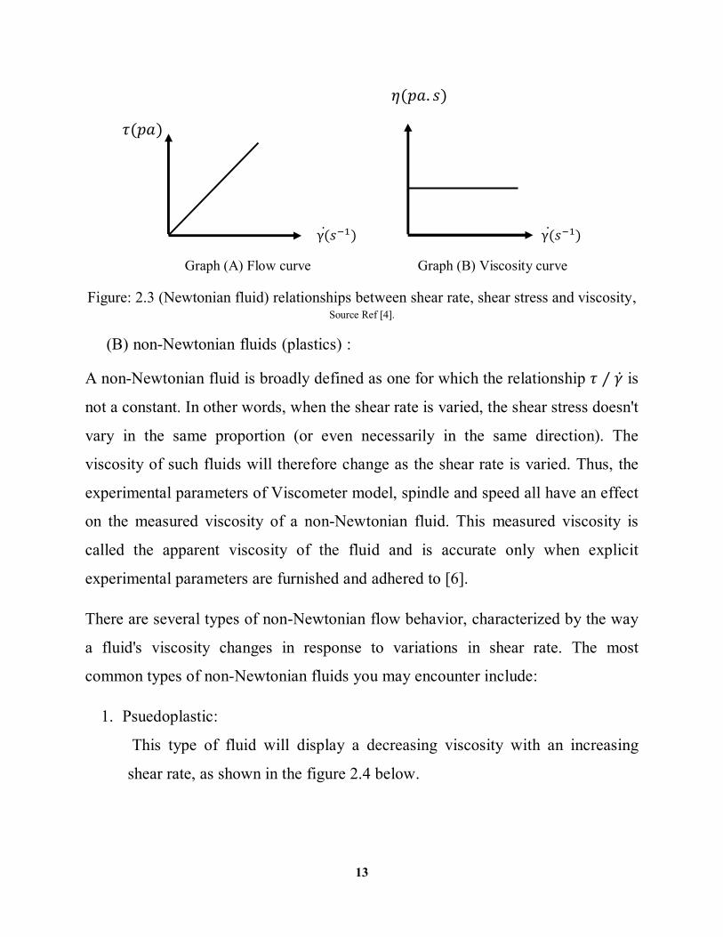
A Newtonian fluid is represented graphically in the figure 2.3 below. The Graph A
shows that the relationship between shear stress (τ) and shear rate (훾) is a straight
line (Flow curve). Graph B shows that the fluid's viscosity remains constant as the
shear rate is varied (Viscosity curve). Typical Newtonian fluids include water and
thin motor oils [4].
13
휂(푝푎. 푠)
휏(푝푎)
γ(푠 ) γ(푠 )
Graph (A) Flow curve Graph (B) Viscosity curve
Figure: 2.3 (Newtonian fluid) relationships between shear rate, shear stress and viscosity, Source Ref [4].
(B) non-Newtonian fluids (plastics) :
A non-Newtonian fluid is broadly defined as one for which the relationship 휏 ⁄ 훾 is
not a constant. In other words, when the shear rate is varied, the shear stress doesn't
vary in the same proportion (or even necessarily in the same direction). The
viscosity of such fluids will therefore change as the shear rate is varied. Thus, the
experimental parameters of Viscometer model, spindle and speed all have an effect
on the measured viscosity of a non-Newtonian fluid. This measured viscosity is
called the apparent viscosity of the fluid and is accurate only when explicit
experimental parameters are furnished and adhered to [6].
There are several types of non-Newtonian flow behavior, characterized by the way
a fluid's viscosity changes in response to variations in shear rate. The most
common types of non-Newtonian fluids you may encounter include:
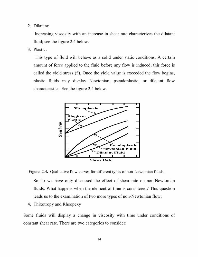
1. Psuedoplastic:
This type of fluid will display a decreasing viscosity with an increasing
shear rate, as shown in the figure 2.4 below.
14
2. Dilatant:
Increasing viscosity with an increase in shear rate characterizes the dilatant
fluid; see the figure 2.4 below.
3. Plastic:
This type of fluid will behave as a solid under static conditions. A certain
amount of force applied to the fluid before any flow is induced; this force is
called the yield stress (f'). Once the yield value is exceeded the flow begins,
plastic fluids may display Newtonian, pseudoplastic, or dilatant flow
characteristics. See the figure 2.4 below.
Figure .2.4. Qualitative flow curves for different types of non-Newtonian fluids.
So far we have only discussed the effect of shear rate on non-Newtonian
fluids. What happens when the element of time is considered? This question
leads us to the examination of two more types of non-Newtonian flow:
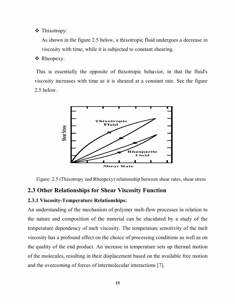
4. Thixotropy and Rheopexy
Some fluids will display a change in viscosity with time under conditions of
constant shear rate. There are two categories to consider:
15
Thixotropy:
As shown in the figure 2.5 below, a thixotropic fluid undergoes a decrease in
viscosity with time, while it is subjected to constant shearing.
Rheopexy:
This is essentially the opposite of thixotropic behavior, in that the fluid's
viscosity increases with time as it is sheared at a constant rate. See the figure
2.5 below.
Figure: 2.5 (Thixotropy and Rheopexy) relationship between shear rates, shear stress
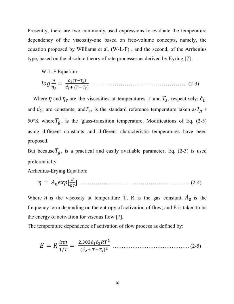
2.3 Other Relationships for Shear Viscosity Function 2.3.1 Viscosity-Temperature Relationships:
An understanding of the mechanism of polymer melt-flow processes in relation to
the nature and composition of the material can be elucidated by a study of the
temperature dependency of melt viscosity. The temperature sensitivity of the melt
viscosity has a profound effect on the choice of processing conditions as well as on
the quality of the end product. An increase in temperature sets up thermal motion
of the molecules, resulting in their displacement based on the available free motion
and the overcoming of forces of intermolecular interactions [7].
16
Presently, there are two commonly used expressions to evaluate the temperature
dependency of the viscosity-one based on free-volume concepts, namely, the
equation proposed by Williams et al. (W-L-F) , and the second, of the Arrhenius
type, based on the absolute theory of rate processes as derived by Eyring [7] .
W-L-F Equation:
푙표푔 = ( ) ( )
……………………………………….. (2-3)
Where휂 and 휂 are the viscosities at temperatures T and푇 , respectively; 푐 :
and 푐 ; are constants; and푇 , is the standard reference temperature taken as푇 +
50°K where푇 , is the 'glass-transition temperature. Modifications of Eq. (2-3)
using different constants and different characteristic temperatures have been
proposed.
But because푇 , is a practical and easily available parameter, Eq. (2-3) is used
preferentially.
Arrhenius-Erying Equation:
휂 = 퐴 푒푥푝[ ] ……………………………………………… (2-4) Where 휂 is the viscosity at temperature T, R is the gas constant, 퐴 is the
frequency term depending on the entropy of activation of flow, and E is taken to be
the energy of activation for viscous flow [7].
The temperature dependence of activation of flow process as defined by:
퐸 = 푅 ⁄ = . ( )
……………………………………. (2-5)
17
2.3.2 viscosity-Pressure Relationship:
Thermoplastic melt viscosity also depends on pressure. Viscosity generally
increases with increasing pressure and can be correlated generally by an equation
of the type [7].
휂 = 퐴 exp(퐵 푝) …………………………………………… (2-6)
Where퐴0 and퐵0; are constants and P is the pressure. The pressure reduces free
volume and, as a result, it reduces molecular mobility; however, this effect
becomes noticeable only at very high pressures. High pressure raises both 푇
and푇 , which also reflects an increase in viscosity. In general, during most
practical situations, thermoplastic melts are assumed incompressible for ease and
simplification.
2.3.3 Viscosity-Molecular Weight Relationship:
Experiments have shown that the following relationship between zero-shear
viscosity and molecular weight holds:
휂 = 퐾 푀 For 푀 <푀 …………………………………….. (2-7) 휂 = 퐾0푀푤
3.5 For 푀 >푀 ……………………...…………….. (2-8) Where 푀 is the critical weight average molecular weight, thought to be the point
at which molecular entanglement begins to dominate the rate of slippage of
molecules [7].
2.3.4 Shear-Rate-Dependent Viscosity Laws :
Several viscosity laws are available for generalized Newtonian flows. The
isothermal viscosity laws will be presented in this section, and Temperature-
18
Dependent Viscosity Laws describes their extension to include temperature
dependence in non isothermal flows [13].
1- Constant For Newtonian fluids, a constant viscosity
휂 = 휂
Can be specified휂 : Is referred to as the Newtonian or zero-shear-rate viscosity.
2- The power law for viscosity is:
휂 = 퐾(휆훾) ……………………………………………………….. (2-9)
Where: K is the consistency factor, λ is the natural time or the reciprocal of a
reference shear rate, and n is the power-law index, which is a property of a given
material.
3- The Bird-Carreau law for viscosity is:
휂 = 휂 +(휂 − 휂 )(1 +휆 훾 ) ……………….……………….. (2-10)
Where:
η = infinite-shear-rate viscosity.
η = zero-shear-rate viscosity.
λ=natural time (i.e., inverse of the shear rate at which the fluid changes from
Newtonian to power-law behavior).
n= power-law index.
The Bird-Carreau law is commonly used when it is necessary to describe the
low-shear-rate behavior of the viscosity. It differs from the Cross law primarily in
the curvature of the viscosity curve in the vicinity of the transition between the
plateau zone and the power law behavior [13].
4- The Cross law for viscosity is:
휂 = ( )
………………………………………………………… (2-11)
19
Where:
휂 = zero-shear-rate viscosity.
λ=natural time (i.e., inverse of the shear rate at which the fluid changes from
Newtonian to power-law behavior).
m= Cross-law index (= 1- n for large shear rates).
Like the Bird-Carreau law, the Cross law is commonly used when it is
necessary to describe the low shear- rate behavior of the viscosity. It differs from
the Bird-Carreau law primarily in the curvature of the viscosity curve in the
vicinity of the transition between the plateau zone and the power law behavior.
5- A modified Cross law for viscosity is also available: 휂 =
( )…………………………………………………………. (2-12)
This law can be considered a special case of the Carreau-Yasuda viscosity law
Eqn. (2-18) where the exponent a has a value of 1.
6- The Bingham law for viscosity is:
휂 = 휂 + ,훾 ≥ 훾
= 휂 + 휏
,훾 < 훾 ……………………………………….. (2-13)
Where:휏 is the yield stress and훾 is the critical shear rate
The Bingham law is commonly used to describe materials such as concrete,
mud, and toothpaste, for which a constant viscosity after a critical shear stress is
a reasonable assumption, typically at rather low shear rates [13].
7- A modified Bingham law for viscosity is also available:
휂 = 휂 + 휏 ( )
……………………………………… (2-14)
20
Where푚 = 3 훾
8- The Herschel-Bulkley law for viscosity is:
휂 = [휏 �
+ K (2 − 푛) + (푛 − 1) , 훾 ≤ 훾
= + 퐾
, 훾 > 훾 …………………………….…..… (2-15)
Where τ is the yield stress, γ is the critical shear rate, K is the consistency factor
and n is the power law index.
9- A modified Herschel-Bulkley law is also available:
휂 = 휏
+ 퐾
…………………………….............. (2-16)
10- The log-log law for viscosity is:
휂 = 휂 10 ⌊ ( ⁄ )⌋ [ ⁄ ] …………….... (2-17)
Where:푎 , 푎 and푎 are the coefficients of the polynomial expression.
11- The Carreau-Yasuda law for viscosity is:
휂 = 휂 +(휂 − 휂 )[1 + (휆훾) ] …………………………… (2-18) Where:
휂 = zero-shear-rate viscosity.
η =infinite-shear-rate viscosity.
λ=natural time (i.e., inverse of the shear rate at which the fluid changes from
Newtonian to power-law behavior).
n= power-law index.
21
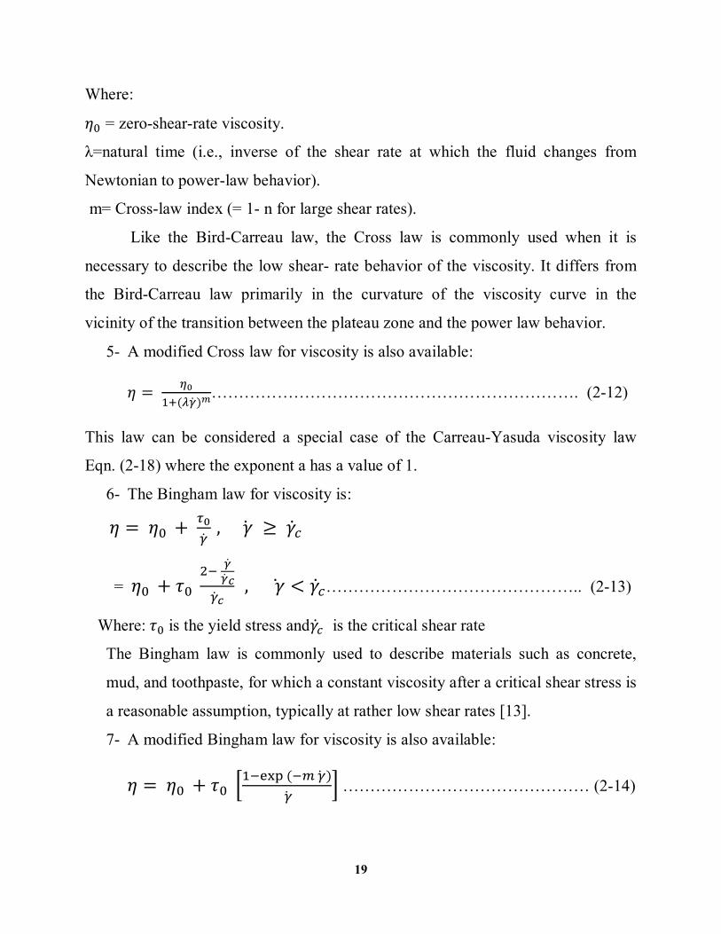
2.4 Rheometers for polymer melt characterization: Rheometry is the measuring arm of rheology and its basic function is to quantify
the rheological material parameters of practical importance [7].
Rheometers used for determining the material functions of thermoplastic melts can
be divided into two broad categories:
(1) Rotational type and
(2) Capillary type
Further, subdivisions are possible and these are shown in Table 2.1. Flow chart 2.1: Rheometers for flow of Thermoplastic Melts
Source: Ref.7
Rheometers for flow of Thermoplastic Melt
Rotational
Unidirectional shear
Cone-N-plate
Oscillatory Shear
Parallel Disk
Capillary
Constant Speed
Plunger Type
Circular
Orifice
Slit Orifice
Screw Extrusion
Type
Circular
Orifice Slit
Orifice
Constant Pressure
Plunger Type
Circular Orifice
Melt Flow Indexer
22
2.5. Processing Polymers: Polymer processing may be divided into two broad areas:
1- The processing of the polymer into some form such as pellets or powder.
2- The process of converting polymeric materials into useful articles of desired
shapes [7].
Our discussion here is restricted to the second method of polymer processing. The
choice of a polymer material for a particular application is often difficult given the
large number of polymer families and even larger number of individual polymers
within each family. However, with a more accurate and complete specification of
end-use requirements and material properties the choice becomes relatively easier.
The problem is then generally reduced to the selection of a material with all the
essential properties in addition to desirable properties and low unit cost. But then
there is usually more than one processing technique for producing a desired item
from polymeric materials or, indeed, a given polymer. For example, hollow plastic
articles like bottles or toys can be fabricated from a number of materials by blow
molding, thermoforming, and rotational molding. The choice of a particular
processing technique is determined by part design, choice of material, production
requirements, and, ultimately, cost–performance considerations.
The most common polymer processing unit operations, but only extrusion and
injection molding, the two predominant polymer processing methods, are treated in
fairly great detail. Our discussion is restricted to general process descriptions only,
with emphasis on the relation between process operating conditions and final
product quality. The subject of polymer processing has been traditionally and
continuously as unite –shaping operations in Table 2.2.
2.5.1 Extrusion:
Extrusion is a processing technique for converting thermoplastic materials in
powdered or granular form into a continuous uniform melt, which is shaped into
23
items of uniform cross-sectional area by forcing it through a die. As shown in
Table 2.2. Extrusion is perhaps the most important plastics processing method
today.
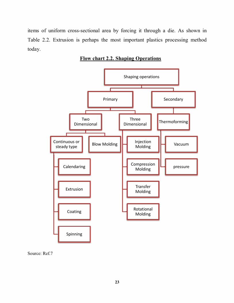
Flow chart 2.2. Shaping Operations
Source: Ref.7
Shaping operations
Primary
Two Dimensional
Continuous or steady type
Calendaring
Extrusion
Coating
Spinning
Blow Molding
Three Dimensional
Injection Molding
Compression Molding
Transfer Molding
Rotational Molding
Secondary
Thermoforming
Vacuum
pressure
24
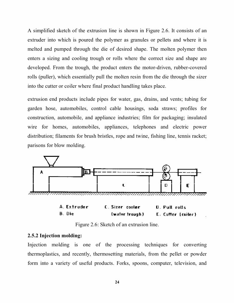
A simplified sketch of the extrusion line is shown in Figure 2.6. It consists of an
extruder into which is poured the polymer as granules or pellets and where it is
melted and pumped through the die of desired shape. The molten polymer then
enters a sizing and cooling trough or rolls where the correct size and shape are
developed. From the trough, the product enters the motor-driven, rubber-covered
rolls (puller), which essentially pull the molten resin from the die through the sizer
into the cutter or coiler where final product handling takes place.
extrusion end products include pipes for water, gas, drains, and vents; tubing for
garden hose, automobiles, control cable housings, soda straws; profiles for
construction, automobile, and appliance industries; film for packaging; insulated
wire for homes, automobiles, appliances, telephones and electric power
distribution; filaments for brush bristles, rope and twine, fishing line, tennis racket;
parisons for blow molding.
Figure 2.6: Sketch of an extrusion line.
2.5.2 Injection molding:
Injection molding is one of the processing techniques for converting
thermoplastics, and recently, thermosetting materials, from the pellet or powder
form into a variety of useful products. Forks, spoons, computer, television, and
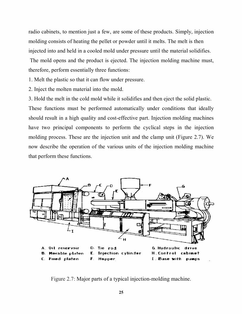
25
radio cabinets, to mention just a few, are some of these products. Simply, injection
molding consists of heating the pellet or powder until it melts. The melt is then
injected into and held in a cooled mold under pressure until the material solidifies.
The mold opens and the product is ejected. The injection molding machine must,
therefore, perform essentially three functions:
1. Melt the plastic so that it can flow under pressure.
2. Inject the molten material into the mold.
3. Hold the melt in the cold mold while it solidifies and then eject the solid plastic.
These functions must be performed automatically under conditions that ideally
should result in a high quality and cost-effective part. Injection molding machines
have two principal components to perform the cyclical steps in the injection
molding process. These are the injection unit and the clamp unit (Figure 2.7). We
now describe the operation of the various units of the injection molding machine
that perform these functions.
Figure 2.7: Major parts of a typical injection-molding machine.
26
2.6. Review of literature:
Throughout the years, research has been intensively going on which various
publications on the melt flow index of plastics materials such as Understanding
Melt Index and ASTM D1238, (Mertz et al, 2013) They use a finite element model
to explore the connections between rheological properties and melt index. We
explore the role of shear thinning by modeling the flow through the melt indexer
using the Bird-Carreau model. They then explore the role of melt viscoelasticity in
the MFI using the co rotational Maxwell model. They presented their results in
dimensionless charts designed to help plastics engineers specify the MFI of a
plastic for an industrial manufacturing process of known material functions [11].
Another study, (S.S. Jikan1 et al, 2013) studied the fabrication and
characterization of polypropylene filled with recycled plaster of paris as filler had
been carried out. Six different percentage levels of filler content were designed
with PP/virgin plaster of paris composite and unfilled PP as reference samples. The
sample characterizations were conducted by using melt density, melt flow index,
tensile test and hardness test. The results demonstrate that the weight percent of
filler content greatly influence the tensile property with decreasing values of
maximum load and elongation at break as well as the melt flow index. However,
the increase in melt density with increasing filler content leads to improve of
hardness values of all samples [13].
There have been a number of rheological models proposed for representing the
flow behavior of polymer melts. The constitutive equations, which relate shear
stress or apparent viscosity with shear rate, involve the use of two to five
parameters. Many of these constitutive equations are quite cumbersome to use in
engineering analyses and hence only a few models are often popular [15]. For
27
example Use of Least Square Procedures and Ansys Polyflow Software to Select
Best Viscosity Model for Polypropylene (Arman Mohamed, Ahmed Ibtahim,
2013) .This work was intended to select the best viscosity model of polypropylene
(PP) data using the percentage root-mean-square error function (PRMSE) and
ansys package. Eleven samples of polypropylene (KPC - PP113) were tested at
different loads and constant temperature 230oC using melt flow index tester (SUST
plastic laboratory) and the results for each sample were recorded. Different
viscosity models (viscosity versus shear rate) were checked using polyflow and the
best of them was selected using PRMSE function. It was found that PP 113 shear
stress versus shear rate was Non-Newtonian and PRMSE beside easy to apply get
an accurate model to quote viscosity [1]. Finally viscosity model Carreau-Yasuda
was best one from them.
28
CHAPTER THREE
MATERIAL AND METHOD
3.1. Introduction:
In this study used Thermoplastic materials were:
1- LDPE (low density polyethylene) (HP 2022: no slip & No Anti block) for
blown film from SABIC (Saudi Arabia Basic Industries corporation).
Typical Applications: Thin shrink film, lamination film, produce bags,
textile packing, soft goods packing and general purpose bags with good
optics and carrier bags.
Typical data:
Table 3-1: The basic characteristics of the used material
Properties unit Value Resin properties
Melt flow rate @1900퐶&2.16 kg load 푔/10푚푖푛. 2 Density @ 230퐶 푘푔 푚⁄ 922
Mechanical Properties Tensile Strength @ break MPa 21 Tensile Elongation @ break % 290 Tensile strength @ yield MPa 8 1% Secant Modulus MPa 160 Dart Impact Strength g 60 Elmendorf Tear strength g 180
Optical Properties Haze % 7 Gloss @ 45 - 80
Thermal softening point Vicat softening point 0퐶 92
Source: Saudi Arabia Basic Industries Corporation (Sabic)
2- Polypropylene (PP) injection grade, MFI = 20 g/10 min, from national petrochemical industrial company.
29
3-2 Method:
Melt Flow rate Index Testing instrument was used. It consists of a heated barrel
and piston assembly to contain a sample of resin. A specified load (weight) is
applied to the piston, and the melted polymer is extruded through a capillary die of
specific dimensions as shown in figure 3-1. The mass of resin, in grams, that is
extruded in 10 minutes equals the MFR; expressed in units of g/10 min. Some
instruments can also calculate the shear rate, shear stress, and viscosity.
Figure 3.1Typical apparatus for determining melt flow rate (showing one of the possible
methods of retaining the die and one type of piston), source Ref: [2].
Testing Procedure:
A small amount of the polymer sample 4grams for (LDPE) and 6 grams for (PP) is
taken in the specially designed MFI apparatus. The apparatus consists of a small
die inserted into the apparatus, with the outside diameter is 9.475mm, inner
diameter is 2.095 mm and the length of die is 8.000mm.The material is packed
30
properly inside the barrel to avoid formation of air pockets. A piston is introduced
which acts as the medium that causes extrusion of the molten polymer. The length
of piston bar is 210mm; piston diameter is 9.475mm.
The sample is preheated for a specified amount of time: 5 min at 190°C for
polyethylene and 6 min at 230°C for polypropylene. After the preheating a
specified weight is introduced into the piston. Examples of standard weights are
2.16 kg to 5 kg. The weight exerts a force on the molten polymer and it
immediately starts flowing through the die. A sample of the melt is taken after
desired period of time and is weighed accurately.
MFI is expressed as grams of polymer/10 minutes of total time of the test.
{Synonyms of Melt Flow Index are Melt Flow Rate and Melt Index. More
commonly used are their abbreviations: MFI, MFR and MI}.
Confusingly, MFR may also indicate "melt flow ratio", the ratio between two melt
flow rates at different gravimetric weights. More accurately, this should be
reported as FRR (flow rate ratio), or simply flow ratio. FRR is commonly used as
an indication of the way in which rheological behavior is influenced by the
molecular mass distribution of the material.
MFI is often used to determine how a polymer will process. However MFI takes no
account of the shear, shear rate or shear history and as such is not a good measure
of the processing window of a polymer. The MFI device is not an extruder in the
conventional polymer processing sense in that there is no screw to compress heat
and shear the polymer. MFI additionally does not take account of long chain
branching nor the differences between shear and elongational rheology. Therefore
two polymers with the same MFI will not behave the same under any given
processing conditions.
31
3.3. Techniques used to calculate mass flow퐆, volume flow퐕, viscosity훈, maximum shear stress 훕퐟and maximum shear rate후퐟:
Most processing technologies of thermoplastic polymers have a phase when the
material is in a fluidic state before formation. This makes possible the completion
of formation with relatively small force and pressure. The knowledge of behavior
and characteristics of melts and the basics of melt rheology are essential for plastic
processing and manufacturing of polymer products [3].
3.3.1 Basics, viscosity law of Newton:
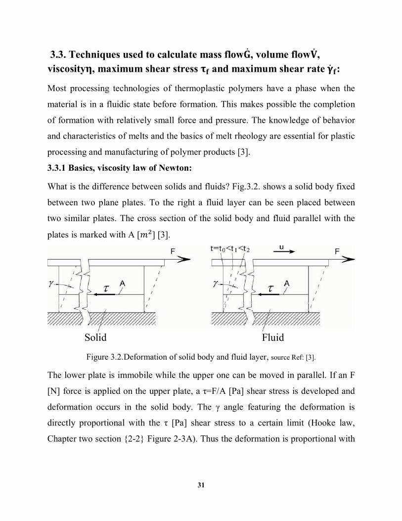
What is the difference between solids and fluids? Fig.3.2. shows a solid body fixed
between two plane plates. To the right a fluid layer can be seen placed between
two similar plates. The cross section of the solid body and fluid parallel with the
plates is marked with A [푚 ] [3].
Solid Fluid
Figure 3.2.Deformation of solid body and fluid layer, source Ref: [3].
The lower plate is immobile while the upper one can be moved in parallel. If an F
[N] force is applied on the upper plate, a τ=F/A [Pa] shear stress is developed and
deformation occurs in the solid body. The γ angle featuring the deformation is
directly proportional with the τ [Pa] shear stress to a certain limit (Hooke law,
Chapter two section {2-2} Figure 2-3A). Thus the deformation is proportional with
32
the shear stress developing in the solid body and the proportionality coefficient is
the G shear elasticity modulus.
퐺 = ………………………………………………………………………..… (3-1)
If there is fluid between the plates, the upper plate moves with a u velocity induced
by the F force, the fluid is under a continuous deformation. Thus in case of fluids
shear rate (푑훾/푑푡) is examined instead of γ deformation.
The basics of fluid mechanics according to Newton model is introduced below.
The Newton model used for describing the behavior of real fluids is the basic
model of melt rheology.
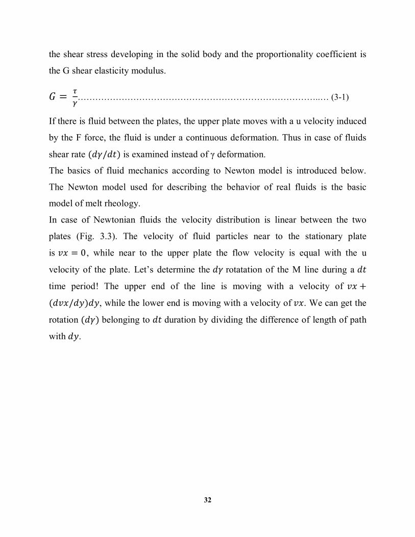
In case of Newtonian fluids the velocity distribution is linear between the two
plates (Fig. 3.3). The velocity of fluid particles near to the stationary plate
is 푣푥 = 0, while near to the upper plate the flow velocity is equal with the u
velocity of the plate. Let’s determine the 푑훾 rotatation of the M line during a 푑푡
time period! The upper end of the line is moving with a velocity of 푣푥 +
(푑푣푥/푑푦)푑푦, while the lower end is moving with a velocity of푣푥. We can get the
rotation (푑훾) belonging to 푑푡 duration by dividing the difference of length of path
with푑푦.
33
Figure: 3.3 Velocity distributions in fluid layer, source Ref: [3].
The time specific angular rotation, i.e. the shear rate is given by dividing with푑푡:
γ = = ……………………………………………………….... (3-2)
We can determine the linear relationship between shear rate and shear stress, the
Newton equation, where 휂[푃푎 · 푠] is a factor depending on fluid properties called
dynamic viscosity:
τ = ηγ = η = η ………………………………………………. (3-3)
The value of η depends on the shear stress required for maintaining a certain shear
rate in case of a given fluid. It should be noted that if 훾& shear rate converges to
zero, shear stress also converges to zero. This means that the static friction of
fluids – in spite of solid materials – is zero.
Another difference is that fluids can be deformed endlessly without the alteration
of their structure.
34
The flow velocity of fluids near to a wall is equal with the velocity of the wall.
This phenomenon is called the law of adherence.
3.3.2 Flow in capillary:
The following chapter is dealing with flow of Newtonian fluids in a small diameter
tube, i.e. capillary, because in the viscosimeter the tested material must pass
through a capillary. Figure 3-4 shows the schema of capillary [3]. Equation (3-3)
and the fact that 훾 shear rate can be expressed with the derivative function of flow
velocity:
τ = ηγ = η ( )………………………………………………………………………….(3-4)
Where 푣(푟)[푚/푠] is the flow velocity of the melt in the function of radial
location 푟[푚] is the radial coordinate of capillary, (0 ≤ 푟 ≤ 푅).
From equation (3-4):
= …………………………………………………………………….. (3-5)
In order to continue the development we have to determine the distribution of
휏shear stress along the cross section of the capillary. The following equation
describes the force equilibrium of a fluid element in the function of푟 radius of the
capillary:
2πr푙τ = r π∆p………………………………………………………………………..….(3-6) Where 훥푝[푃푎] is the pressure difference between the inlet (퐴 ) and outlet (퐴 )
cross section of the capillary, 푙(푚) is the length of the capillary. The force
developing on the surface of푟 radius cylindrical shell is in equilibrium with the
pressure on the r radius base circle of the cylinder (0 ≤ 푟 ≤ 푅).
35
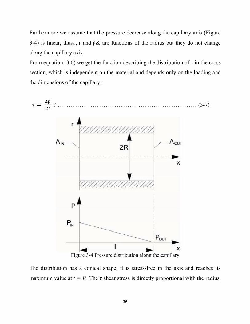
Furthermore we assume that the pressure decrease along the capillary axis (Figure
3-4) is linear, thus휏, 푣and 훾& are functions of the radius but they do not change
along the capillary axis.
From equation (3.6) we get the function describing the distribution of τ in the cross
section, which is independent on the material and depends only on the loading and
the dimensions of the capillary:
τ = ∆ r ………………………………………………………. (3-7)
Figure 3-4 Pressure distribution along the capillary
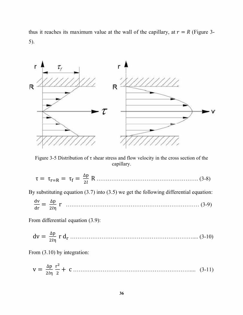
The distribution has a conical shape; it is stress-free in the axis and reaches its
maximum value at푟 = 푅. The 휏 shear stress is directly proportional with the radius,
36
thus it reaches its maximum value at the wall of the capillary, at 푟 = 푅 (Figure 3-
5).
Figure 3-5 Distribution of τ shear stress and flow velocity in the cross section of the capillary.
τ = τ = τ = ∆ R ………………………………………………. (3-8)
By substituting equation (3.7) into (3.5) we get the following differential equation:
= ∆ r ……………………………………………………………… (3-9)
From differential equation (3.9): dv = ∆ rd ………………………………………………………….... (3-10)
From (3.10) by integration:
v = ∆ + c ……………………………………………………….... (3-11)
37
In order to determine constant c we shall use the following boundary condition: At 푟 = 푅:푣 = 0 ………………………………………………………. (3-12)
By substituting the above equation into (3.11):
0 = ∆푙 + c ………………………………………………………… (3-13)
From equation (3.13) we get the value of c:
c = −∆푙
…………………………………………………………… (3-14)
By substituting the value of constant c into equation (3.11) we get the function
describing the distribution of flow velocity in the cross section (Figure 3-5):
v = ∆푙(r −R ) ≤ 0 …………………………………………….. (3-15)
This is a parabolic velocity distribution. The negative sign originates from the fact
that the flow direction and the direction of pressure growth are opposite. In
practice the velocity distribution is calculated from the following equation:
푣 = ∆ (푅 −푟 ) …………………………………………………. (3-16)
3.4 Evaluation of standard test:
The instrument is able to determine Melt Flow Index (MFI) by measuring the mass
of melt which can be calculated by the following equation [2]:
MFI( , ) =.…………………………………………………………………………….(3-17)
Where:
푀퐹퐼[푔/10푚푖푛]; melt flow index,
푇[°퐶]; Test temperature,
퐹[푁]; Weight force,
38
푠[−]; Factor of standard time (10푚푖푛푢푡푒푠 = 600푠), 푠 = 600
푡[푠]; Time needed for V amount of material to flow through the capillary,
푚[푔]; Amount of material flowing through the capillary under t time.
To determine MVR (Melt Volume Rate) volume rate, this can be calculated by the
following equation:
MVR( , ) =.……………………………………………………….(3-18)
Where: 푀푉푅[푐푚 /10푚푖푛]; volume rate,
푇[°퐶]; Test temperature,
퐹[푁]; Weight force,
S [-]; factor of standard time (10푚푖푛푢푡푒푠 = 600푠), 푠 = 600
푡[푠]; Time needed for V amount of material to flow through the capillary,
푉[푐푚 ]; Amount of material flowing through the capillary under 푡time.
3.4.1Evaluation of MFI test:
In case of MFI tests, we apply a simplification, namely we neglect the
pseudoplastic behavior of the polymer melt and we treat it as a Newtonian fluid.
The data required for drawing the viscosity curve can be calculated the following
way [4]:
푉& [푚 /푠] volume flow can be calculated from the MVR by the following
equation:
V =.
…………………………………………………………….. (3-19) Where:
V [푚 /s]; volume flow,
MVR [푐푚 /10 min]; volume flow measured by instrument,
푠 [-]; factor of standard time (10푚푖푛푢푡푒푠 = 600푠), 푠 = 600
Division with 10 is needed to convert [푐푚 ] to [푚 ].
39
MFI can be calculated by equation (3-17).
퐺 [kg/s] mass flow can be calculated from the MFI by the following equation:
G =.
………………………………………………………………. (3-20) Where:
퐺 [kg/s]; mass flow,
MFI [g/10 min]; melt flow index,
푠 [-]; factor of standard time (10푚푖푛푢푡푒푠 = 600푠), 푠 = 600
Division with 10 is needed to convert [푔] to[푘푔].
휌 [kg/m3] density of the melt flow rate can be calculated from 푉&퐺 volume flow
and mass flow:
ρ =.
= ………………………………………………………………………............(3-21)
Where:
L[cm]:pistonmoveddistanceoraveragedistanceofthemeasurement,
m[g}:thesamplequalityofextrusionwhenthepistonmovedL[cm}.
Pressure at inlet cross section of the capillary can be approximated with the
pressure Calculated from D diameter of piston and F force of weight:
∆p = F ……………………………………………………………… (3-22)
Furthermore we assume that according to Figure 3-4 Pressure decreasing is linear
along the capillary axis, thus휏 and 훾 depends on radius but is constant along the
capillary axis.
τ = τ = τ = ∆ R……………………………………………………(3-23)Dynamic viscosity (η) can be calculated by:
μ = .∆ . ……………………………………………………………..… (3-24)
The distribution of 훾 shear rate in the cross section:
40
γ = = ∆ r………………………………………………………………………………… (3-25)
The distribution of 훾 has a shape similar to the τ, because they differ only in a
constant factor. 훾 Reaches its maximum value at the capillary wall.
γ = γ = ∆ R = = γ …………………………… (3-29)
41
CHAPTER FOUR
RESULT AND DISSCUSION
4.1. Introduction:
In this chapter we present our experimental data in many different charts, In
this research used Excel program to draw the data in the form of curves and extract
trend line to draw a curve of power law, activation energy and carreau model.
4.1.1 Low density Polyethylene (LDPE):
a- The result obtained are given in figure 4-1, 4-2 , 4-3& 4-4 and the data is
given in table 4.1,4.2 ,4.3 ,4.4 ,4.5 and 4.6 in Appendix (A).Drawing of
viscosity curve between viscosity versus shear rate and flow curve between
shear stress versus shear rate at different temperatures. The chart shows the
variation of the viscosity and temperature .The higher the temperature the
viscosity decreases and the shear strain rate increases shown in figure 4.1 &
4.2.
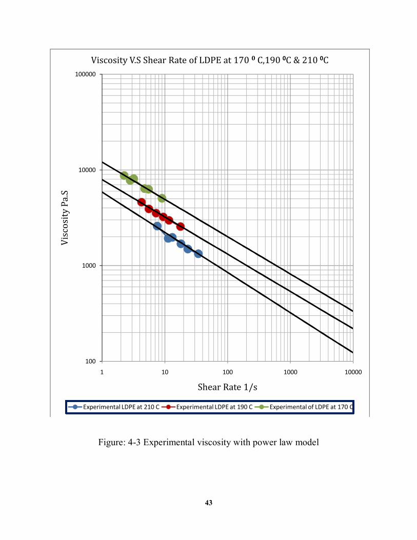
b- Drawing the experimantal data of viscosity with power law shown in figuer
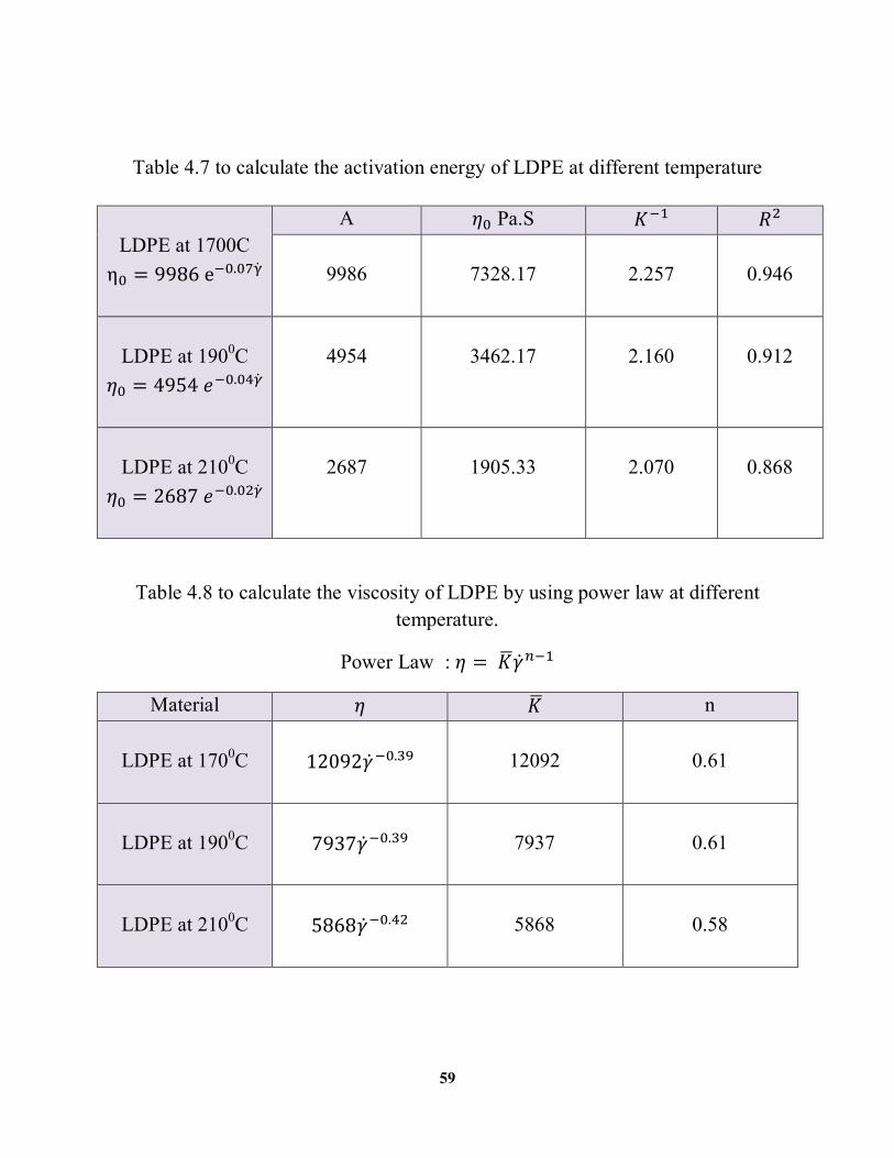
4-3 from figure 4.1Was extracted trendline power law type , the index n for
LDPE at 1700C: n=o.61 , 1900C: n= 0.61 . 2100C: n=0.58.See appendices
(A) table 4.8.
42
Figure: 4-1.Viscosity V.S shear rate curve for (LDPE at 2100C, 1900C & 1700C).
Figure: 4-2. Relation between Shear Stress and Shear Rate for (LDPE at 2100C ,1900C & 1700C).
1
10
100
1000
10000
100000
1 10 100
Visc
osity
Pa.
S
Shear Rate 1/s
Viscosity V.S Shear Rate of LDPE at 170 0 C,190 0C & 210 0C
LDPE at 210 C LDPE at 190 C LDPE at 170 C
0
10000
20000
30000
40000
50000
0 5 10 15 20 25 30 35 40
Shea
r Str
ess P
a
Shear Rate 1/S
Shear Stress V.S Shear rate of LDPE at 2100C,1900C&1700C
Experimental LDPE at 190 C Experimental LDPE at 170 C Experimental LDPE at 210 C
43
Figure: 4-3 Experimental viscosity with power law model
100
1000
10000
100000
1 10 100 1000 10000
Visc
osity
Pa.
S
Shear Rate 1/s
Viscosity V.S Shear Rate of LDPE at 170 0 C,190 0C & 210 0C
Experimental LDPE at 210 C Experimental LDPE at 190 C Experimental of LDPE at 170 C
44
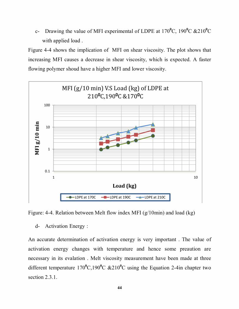
c- Drawing the value of MFI experimental of LDPE at 1700C, 1900C &2100C
with applied load .
Figure 4-4 shows the implication of MFI on shear viscosity. The plot shows that
increasing MFI causes a decrease in shear viscosity, which is expected. A faster
flowing polymer shoud have a higher MFI and lower viscosity.
Figure: 4-4. Relation between Melt flow index MFI (g/10min) and load (kg)
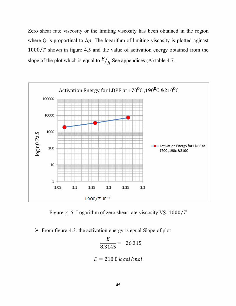
d- Activation Energy :
An accurate determination of activation energy is very important . The value of
activation energy changes with temperature and hence some preaution are
necessary in its evalation . Melt viscosity measurement have been made at three
different temperature 1700C,1900C &2100C using the Equation 2-4in chapter two
section 2.3.1.
0.1
1
10
100
1 10
MFI
g/1
0 m
in
Load (kg)
MFI (g/10 min) V.S Load (kg) of LDPE at 2100C,1900C &1700C
LDPE at 170C LDPE at 190C LDPE at 210C
45
Zero shear rate viscosity or the limiting viscosity has been obtained in the region
where Q is proportinal to ∆푝. The logarithm of limiting viscosity is plotted aginast
1000 푇⁄ shown in figure 4.5 and the value of activation energy obtained from the
slope of the plot which is equal to 퐸 푅.See appendices (A) table 4.7.
Figure .4-5. Logarithm of zero shear rate viscosity VS. 1000 푇⁄
From figure 4.3. the activation energy is egual Slope of plot 퐸
8.3145= 26.315
퐸 = 218.8푘푐푎푙/푚표푙
1
10
100
1000
10000
100000
2.05 2.1 2.15 2.2 2.25 2.3
log
η0 P
a.S
Activation Energy for LDPE at 1700C ,1900C &2100C
Activation Energy for LDPE at 170C ,190c &210C
46
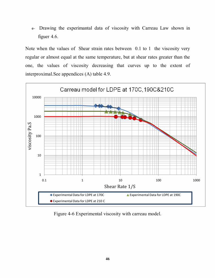
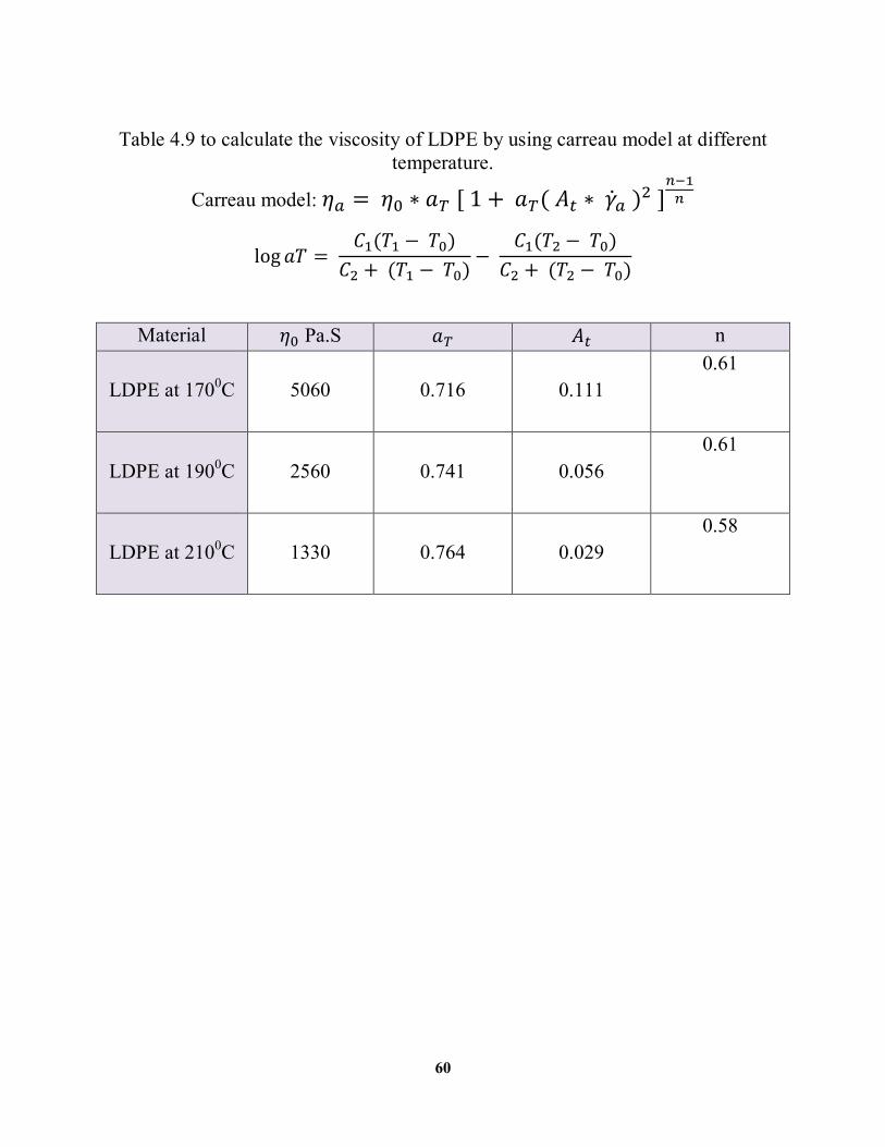
e- Drawing the experimantal data of viscosity with Carreau Law shown in
figuer 4.6.
Note when the values of Shear strain rates between 0.1 to 1 the viscosity very
regular or almost equal at the same temperature, but at shear rates greater than the
one, the values of viscosity decreasing that curves up to the extent of
interproximal.See appendices (A) table 4.9.
Figure 4-6 Experimental viscosity with carreau model.
1
10
100
1000
10000
0.1 1 10 100 1000
visc
osity
Pa.
S
Shear Rate 1/S Experimental Data for LDPE at 170C Experimental Data for LDPE at 190C
Experimental Data for LDPE at 210 C
47
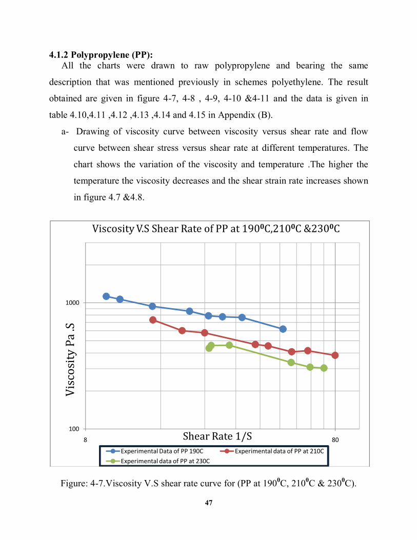
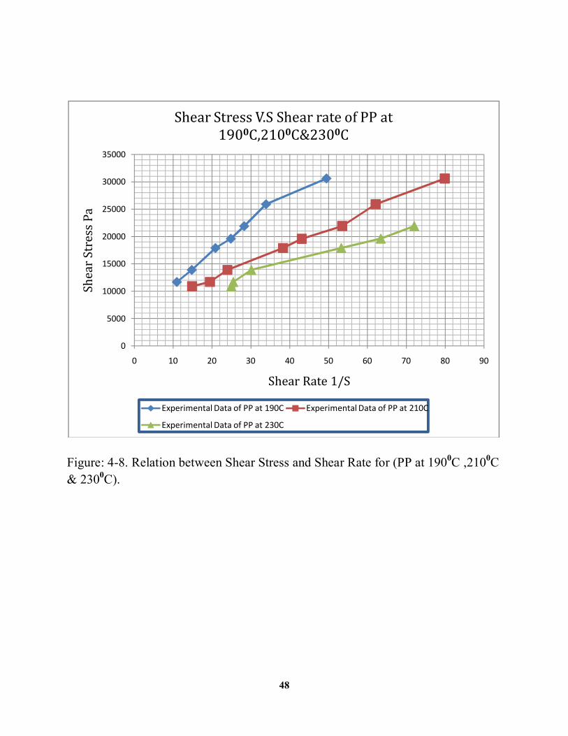
4.1.2 Polypropylene (PP): All the charts were drawn to raw polypropylene and bearing the same
description that was mentioned previously in schemes polyethylene. The result
obtained are given in figure 4-7, 4-8 , 4-9, 4-10 &4-11 and the data is given in
table 4.10,4.11 ,4.12 ,4.13 ,4.14 and 4.15 in Appendix (B).
a- Drawing of viscosity curve between viscosity versus shear rate and flow
curve between shear stress versus shear rate at different temperatures. The
chart shows the variation of the viscosity and temperature .The higher the
temperature the viscosity decreases and the shear strain rate increases shown
in figure 4.7 &4.8.
Figure: 4-7.Viscosity V.S shear rate curve for (PP at 1900C, 2100C & 2300C).
100
1000
8 80
Visc
osity
Pa
.S
Shear Rate 1/S
Viscosity V.S Shear Rate of PP at 1900C,2100C &2300C
Experimental Data of PP 190C Experimental data of PP at 210CExperimental data of PP at 230C
48
Figure: 4-8. Relation between Shear Stress and Shear Rate for (PP at 1900C ,2100C & 2300C).
0
5000
10000
15000
20000
25000
30000
35000
0 10 20 30 40 50 60 70 80 90
Shea
r Str
ess P
a
Shear Rate 1/S
Shear Stress V.S Shear rate of PP at 1900C,2100C&2300C
Experimental Data of PP at 190C Experimental Data of PP at 210C
Experimental Data of PP at 230C
49
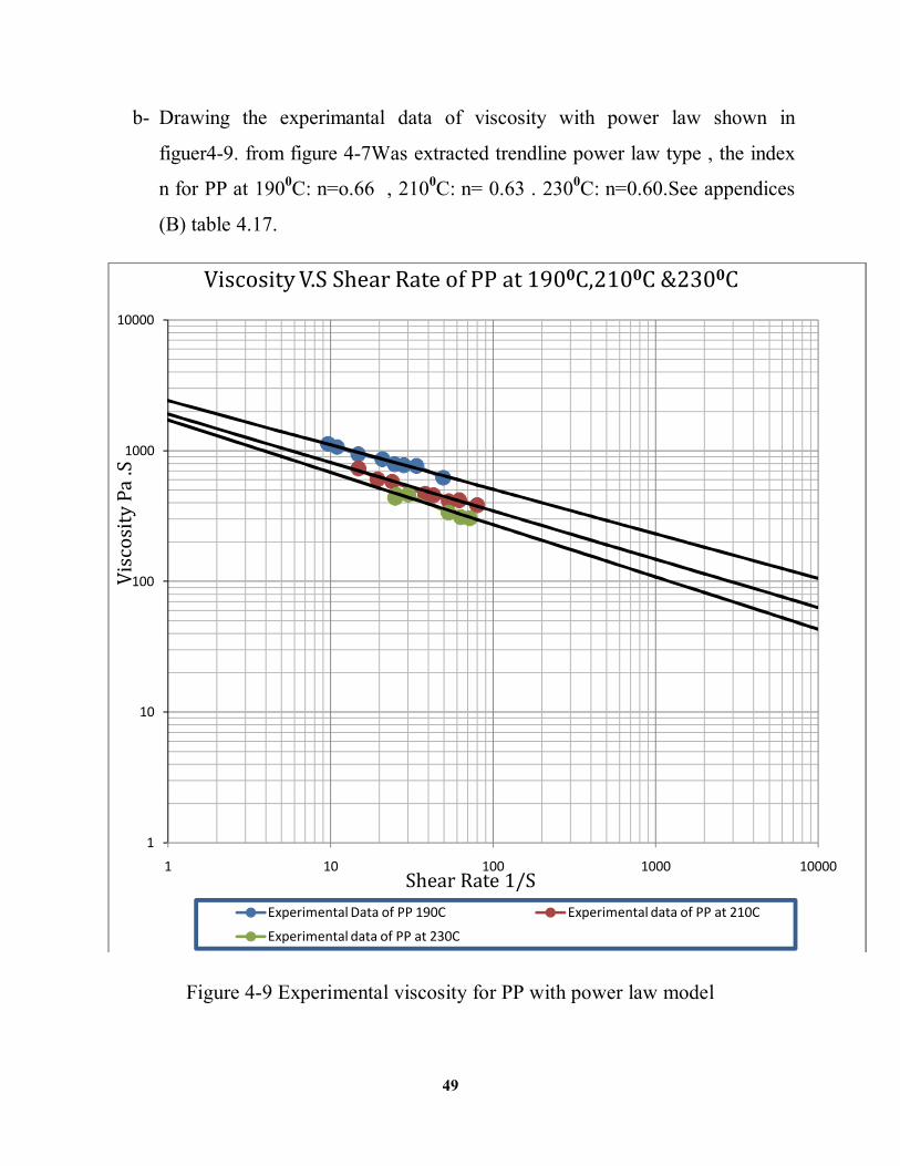
b- Drawing the experimantal data of viscosity with power law shown in
figuer4-9. from figure 4-7Was extracted trendline power law type , the index
n for PP at 1900C: n=o.66 , 2100C: n= 0.63 . 2300C: n=0.60.See appendices
(B) table 4.17.
Figure 4-9 Experimental viscosity for PP with power law model
1
10
100
1000
10000
1 10 100 1000 10000
Visc
osity
Pa
.S
Shear Rate 1/S
Viscosity V.S Shear Rate of PP at 1900C,2100C &2300C
Experimental Data of PP 190C Experimental data of PP at 210C
Experimental data of PP at 230C
50
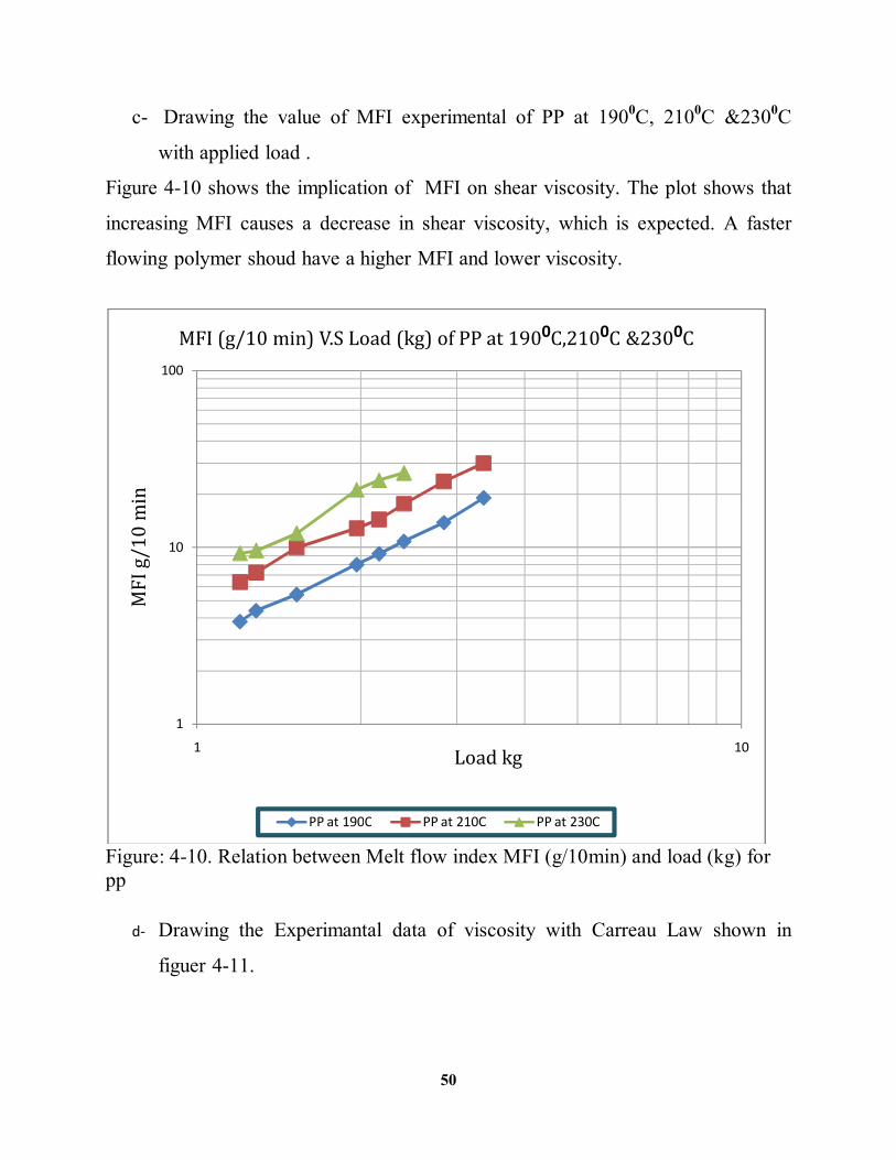
c- Drawing the value of MFI experimental of PP at 1900C, 2100C &2300C
with applied load .
Figure 4-10 shows the implication of MFI on shear viscosity. The plot shows that
increasing MFI causes a decrease in shear viscosity, which is expected. A faster
flowing polymer shoud have a higher MFI and lower viscosity.
Figure: 4-10. Relation between Melt flow index MFI (g/10min) and load (kg) for pp
d- Drawing the Experimantal data of viscosity with Carreau Law shown in
figuer 4-11.
1
10
100
1 10
MFI
g/1
0 m
in
Load kg
MFI (g/10 min) V.S Load (kg) of PP at 1900C,2100C &2300C
PP at 190C PP at 210C PP at 230C
51
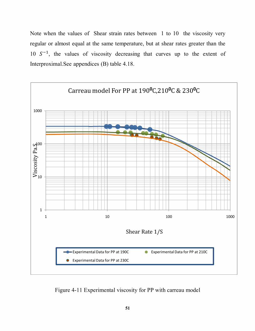
Note when the values of Shear strain rates between 1 to 10 the viscosity very
regular or almost equal at the same temperature, but at shear rates greater than the
10 푆 , the values of viscosity decreasing that curves up to the extent of
Interproximal.See appendices (B) table 4.18.
Figure 4-11 Experimental viscosity for PP with carreau model
1
10
100
1000
1 10 100 1000
Visc
osity
Pa.
S
Shear Rate 1/S
Carreau model For PP at 1900C,2100C & 2300C
Experimental Data for PP at 190C Experimental Data for PP at 210C
Experimental Data for PP at 230C
52
CHAPTER FIVE
CONCLUSIONS AND RECOMMENDATIONS
The Conclusions of this study are summarized as follows:
The melt flow index test is widely used in the industry for quality control purposes
and it is not used for the viscosity study. In this research I tried to study the
viscosity of thermoplastics using MFI.
The melt flow index testing device was used to measure viscosity of
thermoplastics: Polyethylene (PE) and poly propylene (PP) where the MFI is
indirect relation with the shear stress and strain.
In order to get the relation between shear strain rate and viscosity six different
weights are used that is: 2.16, 2.4, 2.84, 3.36, 3.80 and 5 kg for LDPE and eight
different weights are used for PP that is: 1.2, 1.285, 1.525, 1.965, 2.16, 2.40, 2.84
and 3.36kg.
For PE six curves were drawn for the temperature 1700C, 1900C and 2100C the
data for these curves appear in the appendices(A) tables 4.1, 4.2, 4.3, 4.4, 4.5 and
4.6. Similarly for PP six curves were drawn for the temperatures 1900C, 2100C and
2300C the data for these curves appear in the appendices (B) table 4.10, 4.11, 4.12,
4.13, 4.14 and 4.15.
The above data were analyzed and studied to get the parameters in each
rheological model for these:
53
1. Power law model
2. Carreau model
3. Arrhenius model.
These parameters vary with temperature variation. The variations in these
parameters are slight ones.
Further studies are recommended for these parameters to determine whether it is a
fixed value or there is variation that should be considered.
54
REFERENCES
1- Arman Mohammed Abdalla Ahmed , Ahmed Ibrahim Ahmed Sidahmed
Ahmed(2013) “Use of Least Square Procedures and Ansys Polyflow Software
to Select Best Viscosity Model for Polypropylene” Department of Plastic
Engineering, School of Engineering & Technology Industries ,College of
Engineering, Sudan University of Science and Technology, Khartoum P. O.
Box: 72, Sudan.
2- China Educational Instrument & Equipment Corp,"Melt Flow Rate Testing
Instrument guide”. SUST plastic laboratory 2013.
3- John Vlachopoulos& David Strutt. (2001) “The role of rheology in polymer
extrusion,” department of chemical engineering& polydynamics, Inc, Hamilton,
Ontario, Canada.
4- Budapest University of Technology And Economics, Faculty of Mechanical
Engineering, Department of Polymer Engineering,( 2007)“MFI testing-
viscosity measurement of thermoplastic polymers,” 11. February.
5- Dairy processing hand book chapter3.
6- From Wikipedia, the free encyclopedia Journal of Rheology.
7- A.V. SHENOY &D.R.SAIN, “Thermoplastic melt rheology and Processing,”
ch, New York: Marcel Dekker, Inc.
55
8- Tordella, J.P.and Jolly , RE(1953)” Melt Flow of polyethelen measurement by
means of a simple Extrusion plastometer “ Mod. Plast., vol. 31.
9- Polymer Science & Engineering, J. Fried, Prentice Hall.
10- Division of Advanced Materials Science and Engineering, Kongju National
University, Kongju, Chungnam 314701, South Korea (2006)“Determination of
shear viscosity and shear rate from pressure drop and flow rate relationship in a
rectangular channel.
11- Mertz, A. M., Mix, A. W., Baek, H. M., and Giacomin, A. J.( 2013)
“Understanding Melt Index and ASTM D1238,”Journal of Testing and
Evaluation, Vol. 41, No. 1.
12- ASTM D1238-10 (2010) “standard test method for melt flow rates of
thermoplastics by Extrusion plastometer”,Annual Book of ASTM standard,
Vol.8.01,ASTM International , west Conshohocken,.
13- S.S. Jikan1, a, I. Mat Arshat2, b and N.A. Badarulzaman (2013) “Melt Flow
and Mechanical Properties of Polypropylene/Recycled Plaster of Paris” Applied
Mechanics and Materials Vol. 315 pp 905-908.
14- THE ELEMENTS OF Polymer Science and Engineering Second Edition An
Introductory Text and Reference for Engineers aid Chemists. Alfred Rudin
University of Waterloo 1999.
56
APPENDICES A
(Low density polyethylene)
Table 4.1Measured melt flow index for LDPE at 170 0C
Measured Results Sample Load
(Kg) Force
(N) Length (mm)
Time (Sec)
Mass average
(g)
MFI (푔/10푚푖푛)
Density (퐾푔/푚 )
MVR (푐푚 /10푚푖푛)
1 2.16 21.19 5.14 60 0.097 0.97 798 1.22 2 2.40 23.54 6.40 60 .0.12 1.20 791 1.52 3 2.84 27.86 7.33 60 0.153 1.53 885 1.73 4 3.36 32.96 10.94 60 0.20 2.00 771 2.59 5 3.80 37.28 12.57 60 0.25 2.50 839 2.98 6 5.00 49.05 20.57 60 0.40 4.00 821 4.87
Table 4.2Measured melt flow index for LDPE at 190 0C
Measured Results Sample Load
(Kg) Force
(N) Length (mm)
Time (Sec)
Mass average
(g)
MFI (푔/10푚푖푛)
Density (퐾푔/푚 )
MVR (푐푚 /10푚푖푛)
1 2.16 21.19 9.74 60 0.18 1.8 779 2.31 2 2.40 23.54 12.75 60 0.22 2.2 730 3.02 3 2.84 27.86 16.66 60 0.28 2.8 710 3.95 4 3.36 32.96 21.57 60 0.37 3.7 724 5.11 5 3.80 37.28 26.55 60 0.45 4.5 714 6.29 6 5.00 49.05 40.57 60 0.73 7.3 761 9.62
57
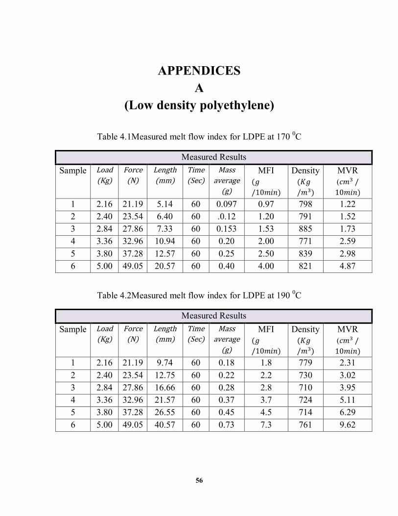
Table 4.3Measured melt flow index for LDPE at 210 0C
Measured Results
Sample Load
(Kg)
Force
(N)
Length
(mm)
Time
(Sec)
Mass
average
(g)
MFI (푔
/10푚푖푛)
Density (퐾푔
/푚 )
MVR
(푐푚 /
10푚푖푛)
1 2.16 21.19 17.08 60 0.32 3.2 780 4.10
2 2.40 23.54 25.37 60 0.39 3.9 639 6.10
3 2.84 27.86 30.00 60 0.53 5.3 746 7.10
4 3.36 32.96 41.46 60 0.65 6.5 665 9.76
5 3.80 37.28 52.97 60 0.95 9.5 759 12.50
6 5.00 49.05 51.81 60 1.35 13.5 732 18.44
Table 4.4 Calculated Results of LDPE at 170 0C
Calculated Results
Sample Force
(N) V
10 (ms)
G
10 (kgs)
∆p
(Mp )
τ
(Mp )
η
(Mp )
γ
(S )
1 21.19 2.03 1.62 0.300 0.01965 0.00873 2.251
2 23.54 2.53 2.00 0.333 0.02181 0.00777 2.807
3 27.86 2.88 2.55 0.395 0.02587 0.00810 3.194
4 32.96 4.32 3.33 0.467 0.03059 0.00639 4.787
5 37.28 4.97 4.17 0.529 0.03465 0.00629 5.509
6 49.05 8.12 6.67 0.696 0.04559 0.00506 9.009
58
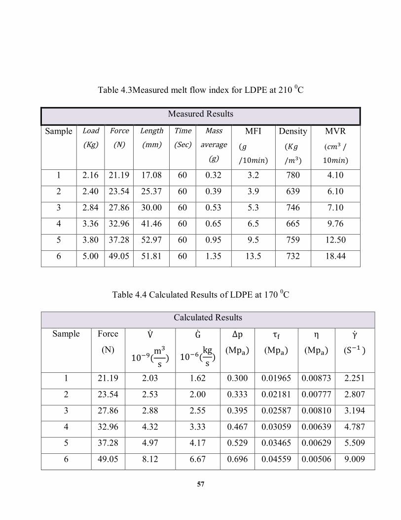
Table 4.5 Calculated Results of LDPE at 190 0C
Calculated Results
Sample Force
(N) V
10 (ms )
G
10 (kgs )
∆p
(Mp )
τ
(Mp )
η
(Mp )
γ
(S )
1 21.19 3.85 3.00 0.300 0.01965 0.00460 4.27
2 23.54 5.03 3.67 0.333 0.02181 0.00391 5.58
3 27.86 6.58 4.67 0.395 0.02587 0.00354 7.25
4 32.96 8.52 6.17 0.467 0.03059 0.00323 9.47
5 37.28 10.50 7.50 0.529 0.03465 0.00292 11.67
6 49.05 16.00 12.17 0.696 0.04559 0.00256 17.81
Table 4.6 Calculated Results of LDPE at 210 0C
Calculated Results
Sample Force
(N) V
10 (ms )
G
10 (kgs )
∆p
(Mp )
τ
(Mp )
η
(Mp )
γ
(S )
1 21.19 6.83 5.33 0.300 0.01965 0.00259 7.59
2 23.54 10.17 6.50 0.333 0.02181 0.00193 11.30
3 27.86 11.83 8.83 0.395 0.02587 0.00197 13.13
4 32.96 16.27 10.83 0.467 0.03059 0.00169 18.10
5 37.28 20.83 15.83 0.529 0.03465 0.00149 23.26
6 49.05 30.73 22.50 0.696 0.04559 0.00133 43.28
59
Table 4.7 to calculate the activation energy of LDPE at different temperature
LDPE at 1700C η = 9986e .
A 휂 Pa.S 퐾 푅
9986
7328.17
2.257
0.946
LDPE at 1900C
휂 = 4954푒 .
4954
3462.17
2.160
0.912
LDPE at 2100C
휂 = 2687푒 .
2687
1905.33
2.070
0.868
Table 4.8 to calculate the viscosity of LDPE by using power law at different temperature.
Power Law : 휂 = 퐾훾
Material 휂 퐾 n
LDPE at 1700C
12092훾 .
12092
0.61
LDPE at 1900C
7937훾 .
7937
0.61
LDPE at 2100C
5868훾 .
5868
0.58
60
Table 4.9 to calculate the viscosity of LDPE by using carreau model at different
temperature.
Carreau model: 휂 = 휂 ∗ 푎 [1 +푎 (퐴 ∗ 훾 ) ]
log 푎푇 = 퐶 (푇 −푇 )
퐶 +(푇 −푇 )−
퐶 (푇 − 푇 )퐶 +(푇 −푇 )
Material 휂 Pa.S 푎 퐴 n
LDPE at 1700C
5060
0.716
0.111
0.61
LDPE at 1900C
2560
0.741
0.056
0.61
LDPE at 2100C
1330
0.764
0.029
0.58
61
APPENDICES B
(Polypropylene)
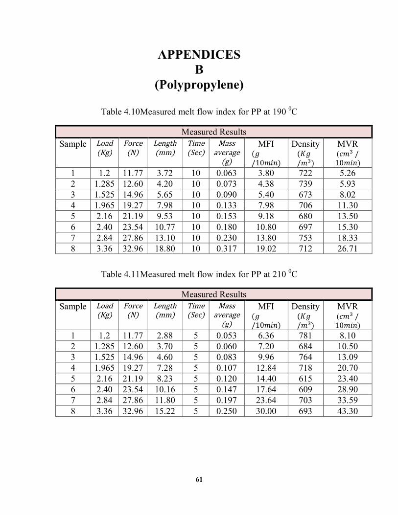
Table 4.10Measured melt flow index for PP at 190 0C
Measured Results Sample Load
(Kg) Force
(N) Length (mm)
Time (Sec)
Mass average
(g)
MFI (푔/10푚푖푛)
Density (퐾푔/푚 )
MVR (푐푚 /10푚푖푛)
1 1.2 11.77 3.72 10 0.063 3.80 722 5.26 2 1.285 12.60 4.20 10 0.073 4.38 739 5.93 3 1.525 14.96 5.65 10 0.090 5.40 673 8.02 4 1.965 19.27 7.98 10 0.133 7.98 706 11.30 5 2.16 21.19 9.53 10 0.153 9.18 680 13.50 6 2.40 23.54 10.77 10 0.180 10.80 697 15.30 7 2.84 27.86 13.10 10 0.230 13.80 753 18.33 8 3.36 32.96 18.80 10 0.317 19.02 712 26.71
Table 4.11Measured melt flow index for PP at 210 0C
Measured Results Sample Load
(Kg) Force
(N) Length (mm)
Time (Sec)
Mass average
(g)
MFI (푔/10푚푖푛)
Density (퐾푔/푚 )
MVR (푐푚 /10푚푖푛)
1 1.2 11.77 2.88 5 0.053 6.36 781 8.10 2 1.285 12.60 3.70 5 0.060 7.20 684 10.50 3 1.525 14.96 4.60 5 0.083 9.96 764 13.09 4 1.965 19.27 7.28 5 0.107 12.84 718 20.70 5 2.16 21.19 8.23 5 0.120 14.40 615 23.40 6 2.40 23.54 10.16 5 0.147 17.64 609 28.90 7 2.84 27.86 11.80 5 0.197 23.64 703 33.59 8 3.36 32.96 15.22 5 0.250 30.00 693 43.30
62
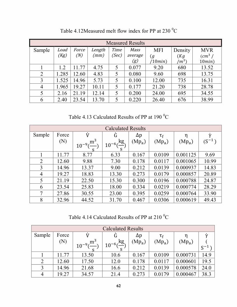
Table 4.12Measured melt flow index for PP at 230 0C
Measured Results Sample Load
(Kg) Force
(N) Length (mm)
Time (Sec)
Mass average
(g)
MFI (푔/10푚푖푛)
Density (퐾푔/푚 )
MVR (푐푚 /10푚푖푛)
1 1.2 11.77 4.75 5 0.077 9.20 680 13.52 2 1.285 12.60 4.83 5 0.080 9.60 698 13.75 3 1.525 14.96 5.73 5 0.100 12.00 735 16.31 4 1.965 19.27 10.11 5 0.177 21.20 738 28.78 5 2.16 21.19 12.14 5 0.200 24.00 695 34.55 6 2.40 23.54 13.70 5 0.220 26.40 676 38.99
Table 4.13 Calculated Results of PP at 190 0C
Calculated Results Sample Force
(N) V
10 (ms)
G
10 (kgs)
∆p (Mp )
τ (Mp )
η (Mp )
γ (S )
1 11.77 8.77 6.33 0.167 0.0109 0.001125 9.69 2 12.60 9.88 7.30 0.178 0.0117 0.001065 10.99 3 14.96 13.37 9.00 0.212 0.0139 0.000937 14.83 4 19.27 18.83 13.30 0.273 0.0179 0.000857 20.89 5 21.19 22.50 15.30 0.300 0.0196 0.000788 24.87 6 23.54 25.83 18.00 0.334 0.0219 0.000774 28.29 7 27.86 30.55 23.00 0.395 0.0259 0.000764 33.90 8 32.96 44.52 31.70 0.467 0.0306 0.000619 49.43
Table 4.14 Calculated Results of PP at 210 0C
Calculated Results Sample Force
(N) V
10 (ms)
G
10 (kgs)
∆p (Mp )
τ (Mp )
η (Mp )
γ (
S ) 1 11.77 13.50 10.6 0.167 0.0109 0.000731 14.9 2 12.60 17.50 12.0 0.178 0.0117 0.000601 19.5 3 14.96 21.68 16.6 0.212 0.0139 0.000578 24.0 4 19.27 34.57 21.4 0.273 0.0179 0.000467 38.3
63
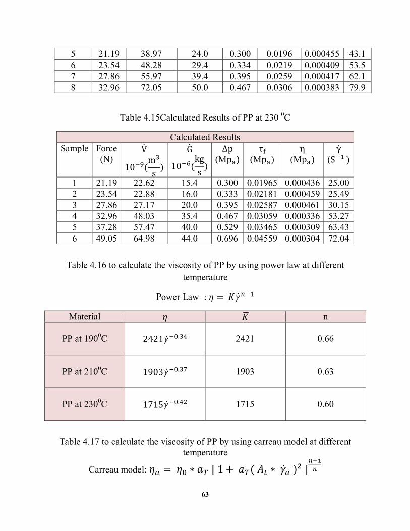
5 21.19 38.97 24.0 0.300 0.0196 0.000455 43.1 6 23.54 48.28 29.4 0.334 0.0219 0.000409 53.5 7 27.86 55.97 39.4 0.395 0.0259 0.000417 62.1 8 32.96 72.05 50.0 0.467 0.0306 0.000383 79.9
Table 4.15Calculated Results of PP at 230 0C
Calculated Results Sample Force
(N) V
10 (ms)
G
10 (kgs)
∆p (Mp )
τ (Mp )
η (Mp )
γ (S )
1 21.19 22.62 15.4 0.300 0.01965 0.000436 25.00 2 23.54 22.88 16.0 0.333 0.02181 0.000459 25.49 3 27.86 27.17 20.0 0.395 0.02587 0.000461 30.15 4 32.96 48.03 35.4 0.467 0.03059 0.000336 53.27 5 37.28 57.47 40.0 0.529 0.03465 0.000309 63.43 6 49.05 64.98 44.0 0.696 0.04559 0.000304 72.04
Table 4.16 to calculate the viscosity of PP by using power law at different
temperature
Power Law : 휂 = 퐾훾
Material 휂 퐾 n
PP at 1900C
2421훾 .
2421
0.66
PP at 2100C
1903훾 .
1903
0.63
PP at 2300C
1715훾 .
1715
0.60
Table 4.17 to calculate the viscosity of PP by using carreau model at different
temperature
Carreau model: 휂 = 휂 ∗ 푎 [1 +푎 (퐴 ∗ 훾 ) ]
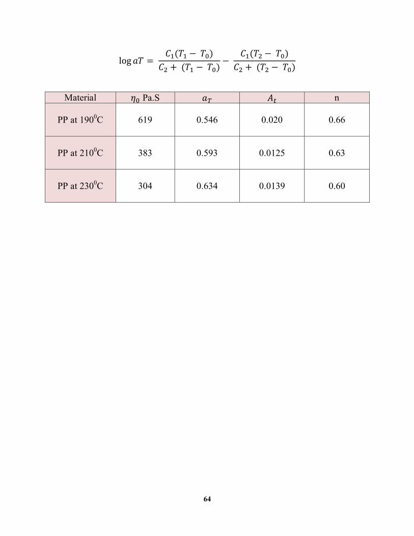
64
log 푎푇 = 퐶 (푇 −푇 )
퐶 +(푇 −푇 )−
퐶 (푇 − 푇 )퐶 +(푇 −푇 )
Material 휂 Pa.S 푎 퐴 n
PP at 1900C
619
0.546
0.020
0.66
PP at 2100C
383
0.593
0.0125
0.63
PP at 2300C
304
0.634
0.0139
0.60