Embed Size (px)
Citation preview

SCIENTIFIC PAPERS
LAND RECLAMATION, EARTH OBSERVATION &SURVEYING, ENVIRONMENTAL ENGINEERING
Series E
Volume VI

LAND RECLAMATION, EARTH OBSERVATION &
SURVEYING, ENVIRONMENTAL ENGINEERING
University of Agronomic Sciencesand Veterinary Medicine of Bucharest
Faculty of Land Reclamationand Environmental Engineering
BucharesT2017
SCIENTIFIC PAPERSSeries E
Volume VI
EDITORIAL BOARD General Editor ‐ Raluca MANEA Executive Editor ‐ Ana VIRSTA
Members: Mariana Catalina CALIN, Carmen CIMPEANU, Veronica IVANESCU, Tatiana IVASUC, Patricia MOCANU, Gabriel POPESCU,
Mirela Alina SANDU, Sevastel MIRCEA, Augustina TRONAC
PUBLISHERS: University of Agronomic Sciences and Veterinary Medicine of Bucharest, Romania ‐
Faculty of Land Reclamation and Environmetal Engineering Address: 5 9 Marasti Blvd., District l, Zip code 011464 Bucharest, Romania
Phone: + 40 213 1830 75, E‐mail: [email protected], Webpage: www.fifim.ro
CERES Publishing House Address: 1 Piața Presei Libere, District l, Zip code 013701, Bucharest, Romania
Phone: + 40 21 317 90 23, E‐mail: [email protected], Webpage: www.editura‐ceres.ro
Copyright 2017 To be cited: Scientific Papers. Series E. LAND RECLAMATION, EARTH
OBSERVATION & SURVEYING, ENVIRONMENTAL ENGINEERING, Vol. VI, 2017
The publishers are not responsible for the content of the scientific papers and opinions published in the Volume. They represent the authorsʹ point of view.
Print ISSN 2285‐6064, CD‐ROM ISSN 2285‐6072, Online ISSN 2393‐5138, ISSN‐L 2285‐6064
International Database Indexing: Index Copernicus; Ulrich’s Periodical Directory (ProQuest); PNB (Polish Scholarly Bibliography); Scientific Indexing Service; Cite Factor (Academic Scientific Journals) Scipio; OCLC; Research Bible
EDITORIAL BOARDGeneral Editor ‐ Raluca MANEAExecutive Editor ‐ Ana VÎRSTA
Members: Mariana Cătălina CĂLIN, Carmen CÎMPEANU,Veronica IVĂNESCU, Tatiana IVASUC, Patricia MOCANU, Gabriel POPESCU,
Mirela Alina SANDU, Sevastel MIRCEA, Augustina TRONAC
SCIENTIFIC & REVIEW COMMITTEE
SCIENTIFIC CHAIRMAN Prof. univ. dr. Sorin Mihai CÎMPEANU
Members*
• Alexandru BADEA - University of Agronomic Sciences and Veterinary Medicine Bucharest, Romania• Ioan BICA - Technical University of Civil Engineering Bucharest, Romania• Daniel BUCUR – “Ion Ionescu de la Brad” University of Agricultural Sciences and Veterinary
Medicine Iasi, Romania• Stefano CASADEI - University of Perugia, Italy• Fulvio CELICO - University of Molise, Italy• Carmen CÎMPEANU - University of Agronomic Sciences and Veterinary Medicine Bucharest,
Romania• Delia DIMITRIU - Manchester Metropolitan University, United Kingdom• Marcel DIRJA - University of Agricultural Sciences and Veterinary Medicine, Cluj, Romania• Claudiu DRAGOMIR - University of Agronomic Sciences and Veterinary Medicine Bucharest,
Romania• Eric DUCLOS-GENDREU - Spot Image, GEO-Information Services, France• Ion GIURMA - Technical University “Gh. Asachi”, Iasi, Romania• Pietro GRIMALDI - University of Bari, Italy• Jean-Luc HORNICK - Faculté de Médecine Vétérinaire, Université de Liège, Belgium• Bela KOVACS - University of Debrecen, Hungary• Ilias KYRIAZAKIS - Newcastle University - United Kingdom• Raluca MANEA - University of Agronomic Sciences and Veterinary Medicine Bucharest, Romania• Florin MĂRĂCINEANU - University of Agronomic Sciences and Veterinary Medicine Bucharest,
Romania• Sevastel MIRCEA - University of Agronomic Sciences and Veterinary Medicine Bucharest, Romania• Nelson PÉREZ-GUERRA - University of Vigo, Spain• John OLDHAM - Scottish Agricultural College, UK• Andreea OLTEANU - University of Agronomic Sciences and Veterinary Medicine Bucharest,
Romania• Maria J. ORUNA-CONCHA - University of Reading, United Kingdom• Marius Ioan PISO - Romanian Space Agency, Romania• Maria POPA – “1 Decembrie 1918” University of Alba Iulia, Romania• Dorin Dumitru PRUNARIU - Romanian Space Agency, Romania• Gabriel POPESCU - University of Agronomic Sciences and Veterinary Medicine Bucharest, Romania• Dan RĂDUCANU - Technical Military Academy of Bucharest, Romania• Jesus SIMAL-GANDARA - University of Vigo, Spain• Ramiro SOFRONIE - University of Agronomic Sciences and Veterinary Medicine Bucharest,
Romania• Marisanna SPERONI - Centro di ricerca per le produzioni foraggere e lattiero-casearie Sede
distaccata di Cremona, Italy• Răzvan Ionuț TEODORESCU - University of Agronomic Sciences and Veterinary Medicine
Bucharest, Romania• Ana TORRADO-AGRASAR - University of Vigo, Spain• Augustina TRONAC - University of Agronomic Sciences and Veterinary Medicine Bucharest,
Romania• Ana VÎRSTA - University of Agronomic Sciences and Veterinary Medicine Bucharest, Romania
*alphabetically ordered by family name

i
Scientific Papers. Series E. Land Reclamation, Earth Observation & Surveying, Environmental Engineering. Vol. VI, 2017Print ISSN 2285-6064, CD-ROM ISSN 2285-6072, Online ISSN 2393-5138, ISSN-L 2285-6064
CONTENTS ENVIRONMENTAL SCIENCE AND ENGINEERING
1. BRIQUETTING OF ROSE OIL PROCESSING WASTES WITH TWO DIFFERENT DIES USING HYDRAULIC PRESS MACHINE, Kamil EKİNCİ, Oral ERTUĞRUL, Haşmet Emre AKMAN, Murat MEMİCİ, Davut AKBOLAT …………………………………………………………………… 1
2. DESIGN AND CONSTRUCTION OF A PILOT SCALE AERATED STATIC PILE COMPOSTING SYSTEMS, Kamil EKİNCİ, İsmail TOSUN, Seyit Ahmet İNAN, Murat MEMICI, Barbaros S. KUMBUL ………………………………………………………………………………………………… 7
3. ENVIRONMENTAL AND TECHNOLOGICAL ASPECTS OF USE OF RESIDUES FROM TOBACCO PRODUCTION AS HEATING FUEL, Dimitar KEHAYOV, Georgi KOMITOV ………. 13
4. EVALUATING OF ELECTRIC ENERGY GENERATING POTENTIAL USING BIOGAS FROM ANIMAL BIOMASSES IN BURDUR CITY, Recep KULCU, Cihannur CIHANALP ……………… 17
5. COMPOSTING OF OPIUM POPPY PROCESSING SOLID WASTE WITH POULTRY MANURE: EFFECTS OF AIRFLOW RATE ON COMPOSTING LOSSES, Barbaros S. KUMBUL, Kamil EKİNCİ, İsmail TOSUN ……….……….……….……….……….……….……….……….………….. 23
6. ENVIRONMENTAL ASSESSMENT ON AN INDUSTRIAL SITE LOCATED IN VRANCEA COUNTY ROMANIA, Patricia MOCANU, Laurentiu MOCANU ……….……….……….………… 31
7. RESEARCHES AND STUDIES REGARDING THE MICROBIAL INDICATORS OF WATER POLLUTION OF CASTAILOR CREEK, BISTRITA, Mihaela ORBAN, Sebastian PLUGARU, Tiberiu RUSU, Rahela CARPA ……….……….……….……….……….……….……….…………… 39
8. ASSESSING THE CONSERVATION STATUS OF FISH SPECIES FROM THE GILORT RIVER PROTECTED AREA, Irina-Ramona PECINGINA, Roxana-Gabriela POPA ……….…………….. 45
9. PHYSICAL-CHEMICAL PROPERTIES ANALYSIS OF THE SOIL CONTAMINATED WITH HEAVY METALS FROM COPSA MICA AREA, Ioana Monica SUR, Alexandra CIMPEAN, Valer MICLE, Claudiu TANASELIA ……….……….……….……….……….……….……….…………… 51
SUSTAINABLE DEVELOPMENT OF RURAL AREA
1. DETERMINATION OF THE AREAS SUITABLE FOR BIOGAS ENERGY PRODUCTION BY USING GEOGRAPHIC INFORMATION SYSTEMS (GIS): EUPHRATES BASIN CASE, Burak SALTUK, Ozan ARTUN, Atilgan A TILGAN ……….……….……….……….……….…………… 57
2. COMPARISON OF THE HEATING ENERGY REQUIREMENTS OF THE GREENHOUSES IN THE TIGRIS BASIN WITH ANTALYA, Burak SALTUK, Nazire MIKAIL, Atilgan ATILGAN, Yusuf AYDIN ……….……….……….……….……….……….……….……….……….……….…… 65
3. LAND RECLAMATION WORKS OPPORTUNITY AND FEASIBILITY IN CLIMATE CHANGE CONTEXT, Dragos DRACEA, Augustina TRONAC, Sebastian MUSTATA ……….…………….. 71
DISASTER MANAGEMENT 1. EX-ANTE AND EX-POST INSTRUMENTAL DIAGNOSIS OF BUILDINGS STRUCTURAL
HEALTH, AN APPROACH AT THE LEVEL OF THE NATIONAL SEISMIC NETWORK, URBAN-INCERC, Claudiu-Sorin DRAGOMIR, Daniela DOBRE, Iolanda-Gabriela CRAIFALEANU, Emil-Sever GEORGESCU ……….……….……….……….……….……….……….……….……….. 77
WATER RESOURCES MANAGEMENT 1. WATER-YIELD RELATIONSHIP OF ZIVZIK POMEGRANATE UNDER DEFICIT IRRIGATION
CONDITIONS, Yusuf AYDIN, Nazire MIKAIL, Mine PAKYÜREK, Burak SALTUK, Mehmet SEVEN ……….……….……….……….……….……….……….……….……….……….…………… 81
2. BENCHMARKING PERFORMANCE OF LARGE SCALE IRRIGATION SCHEMES WITH COMPARATIVE INDICATORS IN TURKEY, Hasan DEĞİRMENCİ, Çağatay TANRIVERDİ, Fırat ARSLAN, Engin GÖNEN ……….……….……….……….……….……….……….……….…. 87
ii
Scientific Papers. Series E. Land Reclamation, Earth Observation & Surveying, Environmental Engineering. Vol. VI, 2017Print ISSN 2285-6064, CD-ROM ISSN 2285-6072, Online ISSN 2393-5138, ISSN-L 2285-6064
3. ASSESSMENT OF EFFECTS OF DIFFERENT IRRIGATION WATER REGIME ON WINTER WHEAT YIELD AND WATER USE EFFICIENCY, Sema KALE ÇELİK, Sevinc MADENOĞLU, Bulent SONMEZ, Kadri AVAG, Ufuk TURKER, Gokhan CAYCI, Cihat KUTUK, Lee HENG … 93
4. COMPARISON BETWEEN TWO PRODUCTION TECHNOLOGIES AND TWO TYPES OF SUBSTRATES IN AN EXPERIMENTAL AQUAPONIC RECIRCULATION SYSTEM, Ivaylo SIRAKOV, Katya VELICHKOVA, Stefka STOYANOVA, Desislava SLAVCHEVA-SIRAKOVA, Yordan STAYKOV ……….……….……….……….……….……….……….…………. 98
5. BIOACUMULATION AND PROTEIN CONTENT OF LEMNA MINUTA KUNTH AND LEMNA VALDIVIANA PHIL. IN BULGARIAN WATER RESERVOIRS, Katya VELICHKOVA, Ivaylo SIRAKOV, Elica VALKOVA, Stefka STOYANOVA, Gergana KOSTADINOVA ……….……….………….. 104
POLLUTION CONTROL, LAND PLANNING 1. STUDY ON PHYSICO-CHEMICAL PROPERTIES OF SOIL IN THE RADES MINE AREA,
Mihaela Adriana BABAU, Valer MICLE, Ioana Monica SUR ……….……….……….…………… 108 2. CONSIDERATIONS OVER CAUSES OF DESERTIFICATION IN BRAILA COUNTY, Catalina
BORDUN (FLOREA-GABRIAN), Sorin Mihai CIMPEANU ……….……….……….……….……. 114 3. EVALUATION OF Cu, Mn AND Zn CONTENT IN PLOUGHED SOIL LAYER, Mihai Teopent
CORCHES, Alina LATO, Maria POPA, Isidora RADULOV, Adina BERBECEA, Florin CRISTA, Lucian NITA, Karel Iaroslav LATO ……….……….……….……….……….……………. 120
4. SEWAGE SLUDGE COMPOSTING AND ITS AGRICULTURAL USE, Valentin FEODOROV …. 124 5. INFLUENCE OF ENVIRONMENTAL CONDITIONS ON LEACHATE BIOSCRUBBERS, Zamfir
PANTER, Mugur BOBE, Gabriela ROSU, Florentina MATEI ……….……….……….………….. 132 6. STUDY ON PEROXIDE VALUES FOR DIFFERENT OILS AND FACTORS AFFECTING THE
QUALITY OF SUNFLOWER OIL, Maria POPA, Ioana GLEVITZKY, Gabriela-Alina DUMITREL, Mirel GLEVITZKY, Dorin POPA ……….……….……….……….……….…………. 137
EARTH OBSERVATION AND GEOGRAPHIC INFORMATION SYSTEMS 1. GEOGRAPHICAL INFORMATION SYSTEMS IN DETERMINATION OF SPATIAL FACTORS IN
CUTANEOUS LEISHMANIASIS CASES DISTRIBUTION, IN ADANA, TURKEY, Ozan ARTUN, Hakan KAVUR ……….……….……….……….……….……….……….……….……….……….…… 141
2. IMPORTANCE OF TOPOLOGY IN A GIS PROJECT OF MONITORING THE SOILS IN AGRICULTURAL LAND, Gabriela BIALI, Paula COJOCARU ……………………………………. 147
3. MAIN FRAMEWORK AND INDICATORS USED IN MAPPING AND ASSESSMENT OF ECOSYSTEM SERVICES FOR THE EU BIODIVERSITY STRATEGY UP TO 2020, Cristina BURGHILA, Sorin Mihai CIMPEANU, Alexandru BADEA ……….……….……….……….……... 155
4. REMOTE SENSING FOR DESERTIFICATION MONITORING IN BRAILA COUNTY, Catalina BORDUN (FLOREA-GABRIAN), Sorin Mihai CIMPEANU ……….……….……….…………….. 163
5. GIS TECHNOLOGY USED FOR FLOODS STUDY, Zoltán FERENCZ, Aurelian Stelian HILA, Sorin Mihai CIMPEANU ……….……….……….……….……….……….……….……….…………. 169
6. MONITORING VEGETATION PHENOLOGYIN THE BRAILA PLAIN USING SENTINEL 2 DATA, Violeta POENARU, Alexandru BADEA, Iulia DANA NEGULA, Cristian MOISE ………. 175
7. INCREASING LAND CLASSIFICATION ACCURACY USING UNMANNED AERIAL VEHICLES (UAVs) WITH MULTISPECTRAL LIDAR SENSOR, Gabriel POPESCU, Octavian Laurentiu BALOTA, Daniela IORDAN ……….……….……….……….……….……….……….……….……… 181
8. RESEARCH INTO THE POTENTIAL OF UTILIZING IMAGE PROCESSING FOR THE EVALUATION OF MAIZE CULTURE, Alexandra TRIF, Mihai GIDEA, Alexandru BOASCA, Sorin Mihai CIMPEANU ……….……….……….……….……….……….……….……….…………. 189
1
Scientific Papers. Series E. Land Reclamation, Earth Observation & Surveying, Environmental Engineering. Vol. VI, 2017Print ISSN 2285-6064, CD-ROM ISSN 2285-6072, Online ISSN 2393-5138, ISSN-L 2285-6064
BRIQUETTING OF ROSE OIL PROCESSING WASTES WITH TWO DIFFERENT DIES USING HYDRAULIC PRESS MACHINE
Kamil EKINCI1, Oral ERTUĞRUL1, Haşmet Emre AKMAN2,
Murat MEMICI1, Davut AKBOLAT1
1Suleyman Demirel University, Isparta, Turkey 2Akdeniz University, Antalya, Turkey
Corresponding author email: [email protected]
Abstract Rose oil processing wastes (ROPW) resulted from water distillation process from petals of R. damascena Mill, which is a by-product of rose oil producing industry leads to environmental problems such as odor and visual pollution. Since these wastes are rich in organic matter, it could be considered as a briquetting material to produce bioenergy. A hydraulic press was used for briquetting process in this study. Two different hexagonal dies with the height of 150 mm were used. No binding material was mixed with ROPW. The resultant briquettes were full hexagonal briquettes with the height of 100 mm and the outer diameter of 60 mm and hollow-core hexagonal briquettes with the height of 100 mm and the outer diameter of 80 mm with 20 mm inner diameter of central hole were produced. All briquettes were stored under ambient conditions for 7 days before testing. Shattering resistance, abrasive resistance, air humidity resistance, water intake resistance tests, thermo-gravimetric analysis, and flue gas emissions (CO2, CO, SO2, and NOX) were performed. The results were discussed in the paper. Key words: briquetting, hexagonal briquettes, rose oil processing wastes. INTRODUCTION Industrial developments in recent years have brought with it the problems of environmental wastes. Elimination or utilization of environmental wastes (industrial, domestic and agricultural) has become inevitable for the modern society. In many developed countries, solid wastes by biomass briquetting are converted to usable, economical and saleable products. Agricultural wastes emerge from agricultural production and agro-industrial operations. Despite being an important source to meet energy needs especially in developing countries, it can be stated that utilization of these wastes are not at the desired level. Briquetting of agricultural wastes or residues is one of the methods used effectively for utilization of biomass. Since agricultural wastes have high moisture content and low density, they are not very efficient for direct combustion in the industrial area or residential heating. Furthermore, the direct use of these wastes is not economical due to transportation, storage and processing operations. In addition, bulk storage of these wastes cause soil, air, water
and visual pollution. Briquetting, compression of sufficiently fragmented materials, improves volumetric heat value and combustion characteristics of biomass, reduces storage costs, decreases particulate emissions to atmospheric, and provides homogenous solid fuel with the same size and shape. Physical properties of briquettes obtained from hydraulic type presses are dependent on the material types, material particle size, moisture content, compaction pressure, the pressure application time, the compression temperature, addition of heating system to the mold and the adhesive materials (Li and Liu, 2000; Suhagar et al., 2006). In order to obtain briquettes with higher shatter resistance, abrasive resistance, water and air resistance, these wastes should be compressed at higher pressure and material with low moisture content and smaller particle size. The addition of heating system to the mold release lignin contained in the biomass and serve as adhesive material. Therefore, the quality of briquettes is improved (Akman and Bilgin, 2012). Rose oil processing wastes (ROPW) are suitable to produce briquettes without adhesive material using hydraulic press
2
Scientific Papers. Series E. Land Reclamation, Earth Observation & Surveying, Environmental Engineering. Vol. VI, 2017Print ISSN 2285-6064, CD-ROM ISSN 2285-6072, Online ISSN 2393-5138, ISSN-L 2285-6064
machine. The resultant briquettes could be utilized in traditional stoves for domestic heating and cooking purposes. In addition, these briquettes can be used in advanced heating systems in the greenhouse (Akman and Bilgin, 2012). This study aimed to determine effects of two different dies on briquetting of rose oil processing wastes using hydraulic press machine. MATERIALS AND METHODS Experiments were carried out in the Department of Agricultural Machinery and Technologies Engineering, Suleyman Demirel University, Biomass Laboratory, Isparta, Turkey. ROPW was received from Biolandes Rose oil Industry and Trade Incorporation Company in Isparta Province. Chemical and physical characteristics of ROPW are given in the Table 1. There was no binding material used for briquetting.
Table 1. Properties of ROPW used in experiment
Properties ROPW Moisture content (wb.,%) 81.68±0.57 Ash content (%) 31.55±1.52 C (%) 49.58±0.11 N (%) 4.92±0.02 S (%) 0.39±0.02 Higher heating value(kcal/kg) 4599.48
The moisture contents of materials were determined using an oven set at 105 ± 1 °C for 24 hours. Ash contents of materials were analyzed based on ISO 1171-1981 at 550 ºC.
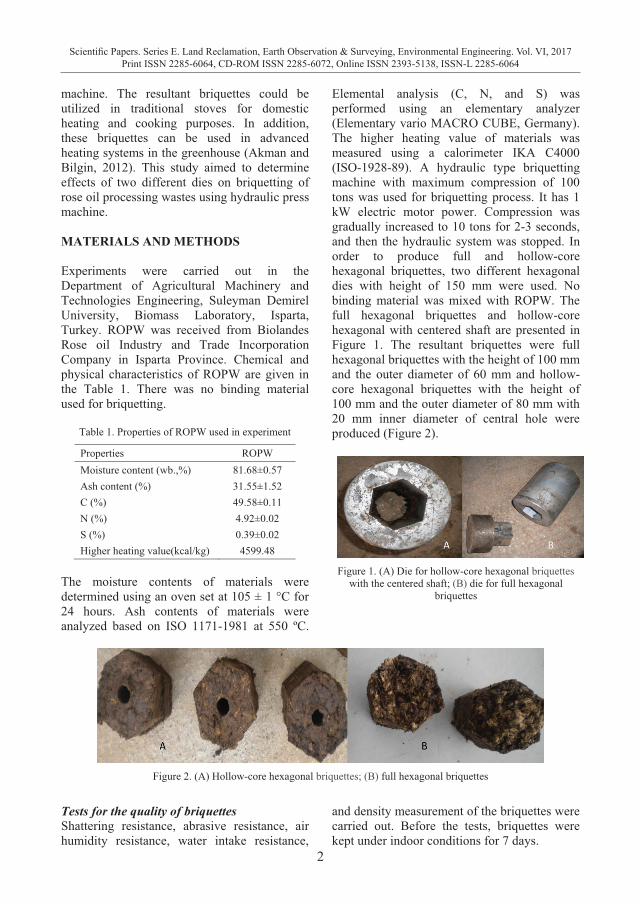
Elemental analysis (C, N, and S) was performed using an elementary analyzer (Elementary vario MACRO CUBE, Germany). The higher heating value of materials was measured using a calorimeter IKA C4000 (ISO-1928-89). A hydraulic type briquetting machine with maximum compression of 100 tons was used for briquetting process. It has 1 kW electric motor power. Compression was gradually increased to 10 tons for 2-3 seconds, and then the hydraulic system was stopped. In order to produce full and hollow-core hexagonal briquettes, two different hexagonal dies with height of 150 mm were used. No binding material was mixed with ROPW. The full hexagonal briquettes and hollow-core hexagonal with centered shaft are presented in Figure 1. The resultant briquettes were full hexagonal briquettes with the height of 100 mm and the outer diameter of 60 mm and hollow-core hexagonal briquettes with the height of 100 mm and the outer diameter of 80 mm with 20 mm inner diameter of central hole were produced (Figure 2).
Figure 1. (A) Die for hollow-core hexagonal briquettes with the centered shaft; (B) die for full hexagonal
briquettes
Figure 2. (A) Hollow-core hexagonal briquettes; (B) full hexagonal briquettes
Tests for the quality of briquettes Shattering resistance, abrasive resistance, air humidity resistance, water intake resistance,
and density measurement of the briquettes were carried out. Before the tests, briquettes were kept under indoor conditions for 7 days.
3
Scientific Papers. Series E. Land Reclamation, Earth Observation & Surveying, Environmental Engineering. Vol. VI, 2017Print ISSN 2285-6064, CD-ROM ISSN 2285-6072, Online ISSN 2393-5138, ISSN-L 2285-6064
machine. The resultant briquettes could be utilized in traditional stoves for domestic heating and cooking purposes. In addition, these briquettes can be used in advanced heating systems in the greenhouse (Akman and Bilgin, 2012). This study aimed to determine effects of two different dies on briquetting of rose oil processing wastes using hydraulic press machine. MATERIALS AND METHODS Experiments were carried out in the Department of Agricultural Machinery and Technologies Engineering, Suleyman Demirel University, Biomass Laboratory, Isparta, Turkey. ROPW was received from Biolandes Rose oil Industry and Trade Incorporation Company in Isparta Province. Chemical and physical characteristics of ROPW are given in the Table 1. There was no binding material used for briquetting.
Table 1. Properties of ROPW used in experiment
Properties ROPW Moisture content (wb.,%) 81.68±0.57 Ash content (%) 31.55±1.52 C (%) 49.58±0.11 N (%) 4.92±0.02 S (%) 0.39±0.02 Higher heating value(kcal/kg) 4599.48
The moisture contents of materials were determined using an oven set at 105 ± 1 °C for 24 hours. Ash contents of materials were analyzed based on ISO 1171-1981 at 550 ºC.
Elemental analysis (C, N, and S) was performed using an elementary analyzer (Elementary vario MACRO CUBE, Germany). The higher heating value of materials was measured using a calorimeter IKA C4000 (ISO-1928-89). A hydraulic type briquetting machine with maximum compression of 100 tons was used for briquetting process. It has 1 kW electric motor power. Compression was gradually increased to 10 tons for 2-3 seconds, and then the hydraulic system was stopped. In order to produce full and hollow-core hexagonal briquettes, two different hexagonal dies with height of 150 mm were used. No binding material was mixed with ROPW. The full hexagonal briquettes and hollow-core hexagonal with centered shaft are presented in Figure 1. The resultant briquettes were full hexagonal briquettes with the height of 100 mm and the outer diameter of 60 mm and hollow-core hexagonal briquettes with the height of 100 mm and the outer diameter of 80 mm with 20 mm inner diameter of central hole were produced (Figure 2).
Figure 1. (A) Die for hollow-core hexagonal briquettes with the centered shaft; (B) die for full hexagonal
briquettes
Figure 2. (A) Hollow-core hexagonal briquettes; (B) full hexagonal briquettes
Tests for the quality of briquettes Shattering resistance, abrasive resistance, air humidity resistance, water intake resistance,
and density measurement of the briquettes were carried out. Before the tests, briquettes were kept under indoor conditions for 7 days.
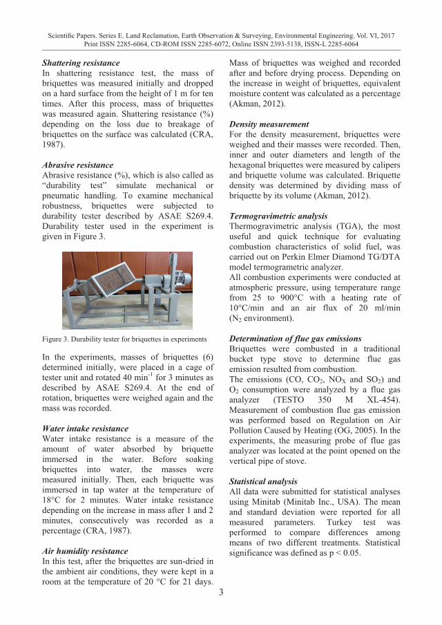
Shattering resistance In shattering resistance test, the mass of briquettes was measured initially and dropped on a hard surface from the height of 1 m for ten times. After this process, mass of briquettes was measured again. Shattering resistance (%) depending on the loss due to breakage of briquettes on the surface was calculated (CRA, 1987). Abrasive resistance Abrasive resistance (%), which is also called as “durability test” simulate mechanical or pneumatic handling. To examine mechanical robustness, briquettes were subjected to durability tester described by ASAE S269.4. Durability tester used in the experiment is given in Figure 3.
Figure 3. Durability tester for briquettes in experiments In the experiments, masses of briquettes (6) determined initially, were placed in a cage of tester unit and rotated 40 min-1 for 3 minutes as described by ASAE S269.4. At the end of rotation, briquettes were weighed again and the mass was recorded. Water intake resistance Water intake resistance is a measure of the amount of water absorbed by briquette immersed in the water. Before soaking briquettes into water, the masses were measured initially. Then, each briquette was immersed in tap water at the temperature of 18°C for 2 minutes. Water intake resistance depending on the increase in mass after 1 and 2 minutes, consecutively was recorded as a percentage (CRA, 1987). Air humidity resistance In this test, after the briquettes are sun-dried in the ambient air conditions, they were kept in a room at the temperature of 20 °C for 21 days.
Mass of briquettes was weighed and recorded after and before drying process. Depending on the increase in weight of briquettes, equivalent moisture content was calculated as a percentage (Akman, 2012). Density measurement For the density measurement, briquettes were weighed and their masses were recorded. Then, inner and outer diameters and length of the hexagonal briquettes were measured by calipers and briquette volume was calculated. Briquette density was determined by dividing mass of briquette by its volume (Akman, 2012). Termogravimetric analysis Thermogravimetric analysis (TGA), the most useful and quick technique for evaluating combustion characteristics of solid fuel, was carried out on Perkin Elmer Diamond TG/DTA model termogrametric analyzer. All combustion experiments were conducted at atmospheric pressure, using temperature range from 25 to 900°C with a heating rate of 10°C/min and an air flux of 20 ml/min (N2 environment). Determination of flue gas emissions Briquettes were combusted in a traditional bucket type stove to determine flue gas emission resulted from combustion. The emissions (CO, CO2, NOX and SO2) and O2 consumption were analyzed by a flue gas analyzer (TESTO 350 M XL-454). Measurement of combustion flue gas emission was performed based on Regulation on Air Pollution Caused by Heating (OG, 2005). In the experiments, the measuring probe of flue gas analyzer was located at the point opened on the vertical pipe of stove. Statistical analysis All data were submitted for statistical analyses using Minitab (Minitab Inc., USA). The mean and standard deviation were reported for all measured parameters. Turkey test was performed to compare differences among means of two different treatments. Statistical significance was defined as p < 0.05.
4
Scientific Papers. Series E. Land Reclamation, Earth Observation & Surveying, Environmental Engineering. Vol. VI, 2017Print ISSN 2285-6064, CD-ROM ISSN 2285-6072, Online ISSN 2393-5138, ISSN-L 2285-6064
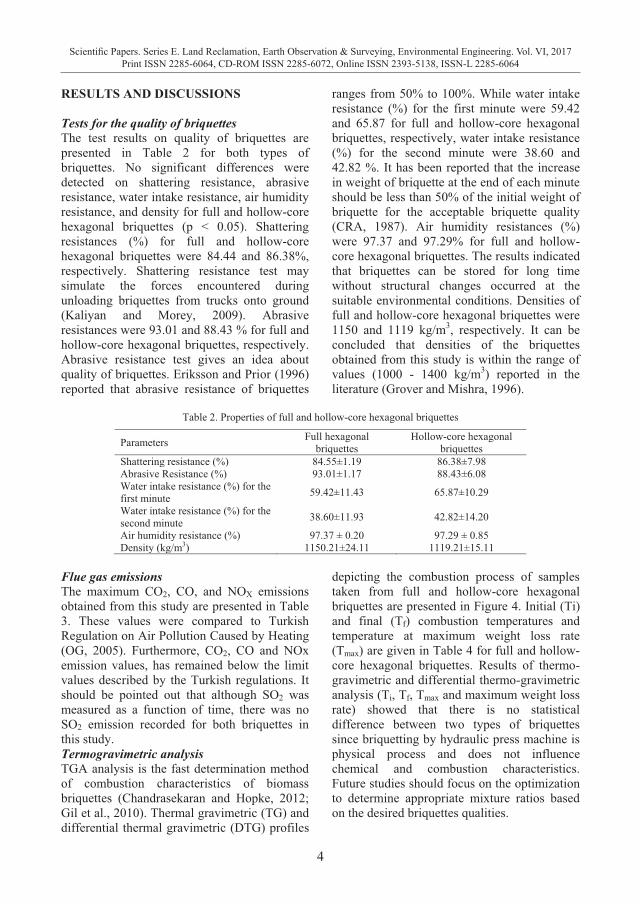
RESULTS AND DISCUSSIONS Tests for the quality of briquettes The test results on quality of briquettes are presented in Table 2 for both types of briquettes. No significant differences were detected on shattering resistance, abrasive resistance, water intake resistance, air humidity resistance, and density for full and hollow-core hexagonal briquettes (p < 0.05). Shattering resistances (%) for full and hollow-core hexagonal briquettes were 84.44 and 86.38%, respectively. Shattering resistance test may simulate the forces encountered during unloading briquettes from trucks onto ground (Kaliyan and Morey, 2009). Abrasive resistances were 93.01 and 88.43 % for full and hollow-core hexagonal briquettes, respectively. Abrasive resistance test gives an idea about quality of briquettes. Eriksson and Prior (1996) reported that abrasive resistance of briquettes
ranges from 50% to 100%. While water intake resistance (%) for the first minute were 59.42 and 65.87 for full and hollow-core hexagonal briquettes, respectively, water intake resistance (%) for the second minute were 38.60 and 42.82 %. It has been reported that the increase in weight of briquette at the end of each minute should be less than 50% of the initial weight of briquette for the acceptable briquette quality (CRA, 1987). Air humidity resistances (%) were 97.37 and 97.29% for full and hollow-core hexagonal briquettes. The results indicated that briquettes can be stored for long time without structural changes occurred at the suitable environmental conditions. Densities of full and hollow-core hexagonal briquettes were 1150 and 1119 kg/m3, respectively. It can be concluded that densities of the briquettes obtained from this study is within the range of values (1000 - 1400 kg/m3) reported in the literature (Grover and Mishra, 1996).
Table 2. Properties of full and hollow-core hexagonal briquettes
Parameters Full hexagonal briquettes
Hollow-core hexagonal briquettes
Shattering resistance (%) 84.55±1.19 86.38±7.98 Abrasive Resistance (%) 93.01±1.17 88.43±6.08 Water intake resistance (%) for the first minute 59.42±11.43 65.87±10.29
Water intake resistance (%) for the second minute 38.60±11.93 42.82±14.20
Air humidity resistance (%) 97.37 ± 0.20 97.29 ± 0.85 Density (kg/m3) 1150.21±24.11 1119.21±15.11
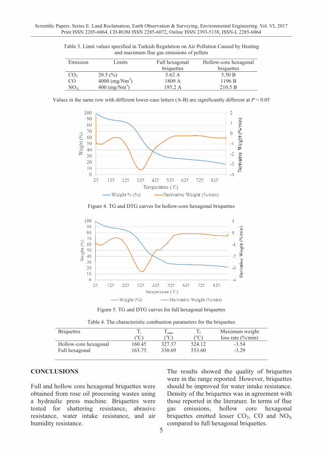
Flue gas emissions The maximum CO2, CO, and NOX emissions obtained from this study are presented in Table 3. These values were compared to Turkish Regulation on Air Pollution Caused by Heating (OG, 2005). Furthermore, CO2, CO and NOx emission values, has remained below the limit values described by the Turkish regulations. It should be pointed out that although SO2 was measured as a function of time, there was no SO2 emission recorded for both briquettes in this study. Termogravimetric analysis TGA analysis is the fast determination method of combustion characteristics of biomass briquettes (Chandrasekaran and Hopke, 2012; Gil et al., 2010). Thermal gravimetric (TG) and differential thermal gravimetric (DTG) profiles
depicting the combustion process of samples taken from full and hollow-core hexagonal briquettes are presented in Figure 4. Initial (Ti) and final (Tf) combustion temperatures and temperature at maximum weight loss rate (Tmax) are given in Table 4 for full and hollow-core hexagonal briquettes. Results of thermo-gravimetric and differential thermo-gravimetric analysis (Ti, Tf, Tmax and maximum weight loss rate) showed that there is no statistical difference between two types of briquettes since briquetting by hydraulic press machine is physical process and does not influence chemical and combustion characteristics. Future studies should focus on the optimization to determine appropriate mixture ratios based on the desired briquettes qualities.
5
Scientific Papers. Series E. Land Reclamation, Earth Observation & Surveying, Environmental Engineering. Vol. VI, 2017Print ISSN 2285-6064, CD-ROM ISSN 2285-6072, Online ISSN 2393-5138, ISSN-L 2285-6064
RESULTS AND DISCUSSIONS Tests for the quality of briquettes The test results on quality of briquettes are presented in Table 2 for both types of briquettes. No significant differences were detected on shattering resistance, abrasive resistance, water intake resistance, air humidity resistance, and density for full and hollow-core hexagonal briquettes (p < 0.05). Shattering resistances (%) for full and hollow-core hexagonal briquettes were 84.44 and 86.38%, respectively. Shattering resistance test may simulate the forces encountered during unloading briquettes from trucks onto ground (Kaliyan and Morey, 2009). Abrasive resistances were 93.01 and 88.43 % for full and hollow-core hexagonal briquettes, respectively. Abrasive resistance test gives an idea about quality of briquettes. Eriksson and Prior (1996) reported that abrasive resistance of briquettes
ranges from 50% to 100%. While water intake resistance (%) for the first minute were 59.42 and 65.87 for full and hollow-core hexagonal briquettes, respectively, water intake resistance (%) for the second minute were 38.60 and 42.82 %. It has been reported that the increase in weight of briquette at the end of each minute should be less than 50% of the initial weight of briquette for the acceptable briquette quality (CRA, 1987). Air humidity resistances (%) were 97.37 and 97.29% for full and hollow-core hexagonal briquettes. The results indicated that briquettes can be stored for long time without structural changes occurred at the suitable environmental conditions. Densities of full and hollow-core hexagonal briquettes were 1150 and 1119 kg/m3, respectively. It can be concluded that densities of the briquettes obtained from this study is within the range of values (1000 - 1400 kg/m3) reported in the literature (Grover and Mishra, 1996).
Table 2. Properties of full and hollow-core hexagonal briquettes
Parameters Full hexagonal briquettes
Hollow-core hexagonal briquettes
Shattering resistance (%) 84.55±1.19 86.38±7.98 Abrasive Resistance (%) 93.01±1.17 88.43±6.08 Water intake resistance (%) for the first minute 59.42±11.43 65.87±10.29
Water intake resistance (%) for the second minute 38.60±11.93 42.82±14.20
Air humidity resistance (%) 97.37 ± 0.20 97.29 ± 0.85 Density (kg/m3) 1150.21±24.11 1119.21±15.11
Flue gas emissions The maximum CO2, CO, and NOX emissions obtained from this study are presented in Table 3. These values were compared to Turkish Regulation on Air Pollution Caused by Heating (OG, 2005). Furthermore, CO2, CO and NOx emission values, has remained below the limit values described by the Turkish regulations. It should be pointed out that although SO2 was measured as a function of time, there was no SO2 emission recorded for both briquettes in this study. Termogravimetric analysis TGA analysis is the fast determination method of combustion characteristics of biomass briquettes (Chandrasekaran and Hopke, 2012; Gil et al., 2010). Thermal gravimetric (TG) and differential thermal gravimetric (DTG) profiles
depicting the combustion process of samples taken from full and hollow-core hexagonal briquettes are presented in Figure 4. Initial (Ti) and final (Tf) combustion temperatures and temperature at maximum weight loss rate (Tmax) are given in Table 4 for full and hollow-core hexagonal briquettes. Results of thermo-gravimetric and differential thermo-gravimetric analysis (Ti, Tf, Tmax and maximum weight loss rate) showed that there is no statistical difference between two types of briquettes since briquetting by hydraulic press machine is physical process and does not influence chemical and combustion characteristics. Future studies should focus on the optimization to determine appropriate mixture ratios based on the desired briquettes qualities.
Table 3. Limit values specified in Turkish Regulation on Air Pollution Caused by Heating and maximum flue gas emissions of pellets
Emission Limits Full hexagonal briquettes
Hollow-core hexagonal briquettes
CO2 20.5 (%) 5.62 A 5.50 B CO 4000 (mg/Nm3) 1809 A 1196 B NOX 400 (mg/Nm3) 195.2 A 210.5 B
Values in the same row with different lower-case letters (A-B) are significantly different at P < 0.05
Figure 4. TG and DTG curves for hollow-core hexagonal briquettes
Figure 5. TG and DTG curves for full hexagonal briquettes
Table 4. The characteristic combustion parameters for the briquettes
Briquettes Ti (oC)
Tmax(oC)
Tf (oC)
Maximum weightloss rate (%/min)
Hollow-core hexagonal 160.45 327.37 524.12 -3.54 Full hexagonal 163.75 330.69 553.60 -3.29
CONCLUSIONS Full and hollow core hexagonal briquettes were obtained from rose oil processing wastes using a hydraulic press machine. Briquettes were tested for shattering resistance, abrasive resistance, water intake resistance, and air humidity resistance.
The results showed the quality of briquettes were in the range reported. However, briquettes should be improved for water intake resistance. Density of the briquettes was in agreement with those reported in the literature. In terms of flue gas emissions, hollow core hexagonal briquettes emitted lesser CO2, CO and NOX compared to full hexagonal briquettes.
6
Scientific Papers. Series E. Land Reclamation, Earth Observation & Surveying, Environmental Engineering. Vol. VI, 2017Print ISSN 2285-6064, CD-ROM ISSN 2285-6072, Online ISSN 2393-5138, ISSN-L 2285-6064
The maximum emission recorded was in accordance with Turkish regulation. As for thermo-gravimetric analysis of briquettes, both of them yielded similar results. In conclusion, the briquettes can be burned in a traditional stove and advanced combustion system for greenhouse heating and residential heating. Additionally, the briquettes can be used in combined heat and power system as source of biomass. REFERENCES Akman H. E. and Bilgin S. 2012. Pamuk saplarının
hidrolik tip preste briketlemesi üzerine bir çalışma. 27. Ulusal Tarımsal Mekanizasyon Kongresi 2012, Samsun.
Akman H.E., 2012. A Research on the briquetting of Rose Oil (Rosa Damascena Mill.) Distillation Wastes (in Turkish). Master Thesis Akdeniz University.
Chandrasekaran, S.R. and Hopke, P.K. 2012. Kinetics of switch grass pellet thermal decomposition under inert and oxidizing atmospheres. Bioresour. Technol. 125, 52–58.
CRA, 1987. The la densification de la biomass. Commission des Communuates Europeennes. Centre de Recherches Agronomiques.
Eriksson S. and Prior M. 1990. The briquetting of agricultural wastes for fuel. FAO Environment and Energy Paper 11, FAO of the UN, Rome.
Gil M.V., Oulego, P., Casal, M.D., Pevida, C., Pis, J.J., Rubiera, F., 2010. Mechanical durability and combustion characteristics of pellets from biomass blends. Bioresour. Technol. 101 (22), 8859–8867.
Grover P.D. and Mishra, S.K. 1996. Biomass Briquetting: Technology and Practices. Bangkok.
Kaliyan N. and Morey, R.V. 2009. Factors affecting strength and durability of densified biomass products. Biomass and Bioenergy, 33: 337-359.
Li Y. and H. Liu, 2000. High-pressure densification of wood residues to form an upgraded fuel. Biomass and Bioenergy, 19: 177-186.
OG, 2005. Regulation on Air Pollution Caused by Heating (In Turkish). Republic of Turkey, Official Gazette, No: 25699.
Suhagar M., Lope, G.T. and Shahab S. 2006. Specific energy requirement for compacting corn stover. Bioresource Technology, 97: 1420-1426.
7
Scientific Papers. Series E. Land Reclamation, Earth Observation & Surveying, Environmental Engineering. Vol. VI, 2017Print ISSN 2285-6064, CD-ROM ISSN 2285-6072, Online ISSN 2393-5138, ISSN-L 2285-6064
The maximum emission recorded was in accordance with Turkish regulation. As for thermo-gravimetric analysis of briquettes, both of them yielded similar results. In conclusion, the briquettes can be burned in a traditional stove and advanced combustion system for greenhouse heating and residential heating. Additionally, the briquettes can be used in combined heat and power system as source of biomass. REFERENCES Akman H. E. and Bilgin S. 2012. Pamuk saplarının
hidrolik tip preste briketlemesi üzerine bir çalışma. 27. Ulusal Tarımsal Mekanizasyon Kongresi 2012, Samsun.
Akman H.E., 2012. A Research on the briquetting of Rose Oil (Rosa Damascena Mill.) Distillation Wastes (in Turkish). Master Thesis Akdeniz University.
Chandrasekaran, S.R. and Hopke, P.K. 2012. Kinetics of switch grass pellet thermal decomposition under inert and oxidizing atmospheres. Bioresour. Technol. 125, 52–58.
CRA, 1987. The la densification de la biomass. Commission des Communuates Europeennes. Centre de Recherches Agronomiques.
Eriksson S. and Prior M. 1990. The briquetting of agricultural wastes for fuel. FAO Environment and Energy Paper 11, FAO of the UN, Rome.
Gil M.V., Oulego, P., Casal, M.D., Pevida, C., Pis, J.J., Rubiera, F., 2010. Mechanical durability and combustion characteristics of pellets from biomass blends. Bioresour. Technol. 101 (22), 8859–8867.
Grover P.D. and Mishra, S.K. 1996. Biomass Briquetting: Technology and Practices. Bangkok.
Kaliyan N. and Morey, R.V. 2009. Factors affecting strength and durability of densified biomass products. Biomass and Bioenergy, 33: 337-359.
Li Y. and H. Liu, 2000. High-pressure densification of wood residues to form an upgraded fuel. Biomass and Bioenergy, 19: 177-186.
OG, 2005. Regulation on Air Pollution Caused by Heating (In Turkish). Republic of Turkey, Official Gazette, No: 25699.
Suhagar M., Lope, G.T. and Shahab S. 2006. Specific energy requirement for compacting corn stover. Bioresource Technology, 97: 1420-1426.
DESIGN AND CONSTRUCTION OF A PILOT SCALE AERATED
STATIC PILE COMPOSTING SYSTEMS
Kamil EKINCI, Ismail TOSUN, Seyit Ahmet INAN, Murat MEMICI, Barbaros S. KUMBUL
Suleyman Demirel University, 32260 Isparta, Turkey
Corresponding author email: [email protected]
Abstract
The amount of agricultural and industrial wastes is increasing due to increase in industrial and agricultural activities in the world. Therefore, sustainable management of wastes, which is a major challenge being faced by both agricultural and industrial sectors in the world, is required. Composting, which is one of the valorization methods used to accelerate decomposition and stabilization of organic wastes, is well known and getting widespread. This study covers design and instrumentation of a pilot scale aerated static pile composting systems based on engineering principles. With this system, basic scientific data (decomposition rates of composting materials, optimum temperature and moisture values) which are required for construction of large-scale composting facilities and operation of composting process will be obtained. The system consists of (1) aeration system, (2) control, data acquisition and recording unit, and (3) measurement system (temperature, instant CO2/O2 concentrations, airflow, and energy consumption by aeration). In this study, each components of this system will be introduced. This study has been conducted under the program of 1007 of the scientific and technological research council of Turkey.
Key words: aerated static pile composting, composting, instrumentation. INTRODUCTION Sustainable management of wastes is a major challenge for the environment. Composting is one of the most important valorization methods for agricultural waste materials. Several studies have demonstrated that composting could be a suitable low-cost strategy for the recycling of wastes (Keener et al., 2014). Composting is a decomposition of organic materials and a process of which physical, chemical, and biological factors interact simultaneously. At the end of composting process, the new and economic products (humus like materials) are produced (Keener et al., 2000). Compost is used in open fields, orchards, vineyards, urban landscapes, and nursery to improve soil ferti-lity, to increase water holding capacity of soils, and to prepare potting mixes. Composting tech-nology step forward in Turkey among the waste utilization and disposal methods (incineration, land filling etc.,) due to low organic matter content in agricultural soil, erosion control, the need for land rehabilitation in agricultural areas, and wide lands to be forested. Aerated static pile composting method is widespread in the world. Aerated static pile composting is performed with air blower. The process can be
controlled directly using blowers and larger piles can be created. The bulk material is not returned or not mixed form. In general terms, the composting process with aerated static pile method is faster and results in higher quality composts (Stentiford, 1996). Keener et al. (1993) noted “optimization of a design, whe-ther based on cost of construction and opera-tion, energy use (conservation of resources) or pollution levels (odors, dust, etc.) can be done through field experimentation. Field experi-mentation implies collection of basic informa-tion for real working systems (pilot or full scale) and evaluation of the results. Evaluation of how system design and management affects time to reach compost stability is critical to optimizing the process. Therefore, this study focused on design and construction of a pilot scale aerated static pile composting systems for field experimentation of composting process. MATERIALS, METHODS, RESULTS AND DISCUSSIONS Pilot scale aerated static pile composting system The pilot scale aerated static pile composting systems with the annual processing capacity of
8
Scientific Papers. Series E. Land Reclamation, Earth Observation & Surveying, Environmental Engineering. Vol. VI, 2017Print ISSN 2285-6064, CD-ROM ISSN 2285-6072, Online ISSN 2393-5138, ISSN-L 2285-6064
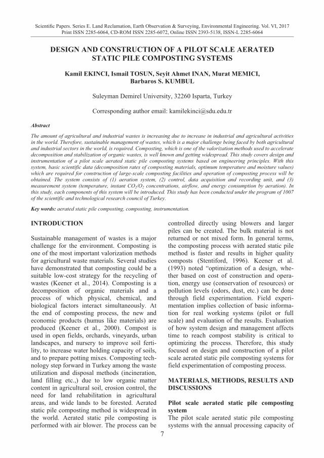
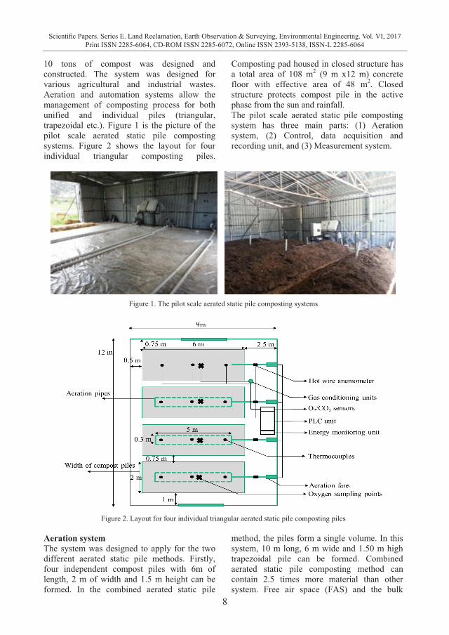
10 tons of compost was designed and constructed. The system was designed for various agricultural and industrial wastes. Aeration and automation systems allow the management of composting process for both unified and individual piles (triangular, trapezoidal etc.). Figure 1 is the picture of the pilot scale aerated static pile composting systems. Figure 2 shows the layout for four individual triangular composting piles.
Composting pad housed in closed structure has a total area of 108 m2 (9 m x12 m) concrete floor with effective area of 48 m2. Closed structure protects compost pile in the active phase from the sun and rainfall. The pilot scale aerated static pile composting system has three main parts: (1) Aeration system, (2) Control, data acquisition and recording unit, and (3) Measurement system.
Figure 1. The pilot scale aerated static pile composting systems
Figure 2. Layout for four individual triangular aerated static pile composting piles
Aeration system The system was designed to apply for the two different aerated static pile methods. Firstly, four independent compost piles with 6m of length, 2 m of width and 1.5 m height can be formed. In the combined aerated static pile
method, the piles form a single volume. In this system, 10 m long, 6 m wide and 1.50 m high trapezoidal pile can be formed. Combined aerated static pile composting method can contain 2.5 times more material than other system. Free air space (FAS) and the bulk

9
Scientific Papers. Series E. Land Reclamation, Earth Observation & Surveying, Environmental Engineering. Vol. VI, 2017Print ISSN 2285-6064, CD-ROM ISSN 2285-6072, Online ISSN 2393-5138, ISSN-L 2285-6064
density of raw materials are determining factor for selection of methods. The aeration fan and the air distribution units to be used in both methods is the same. Aeration fans, each with a 0.5 horsepower electric motor and an air capacity of 1000 m3/h supply air to the compost piles. 50 mm PVC pipes for distributing air were installed under the piles. The schematic layout and appearance of the ventilating pipes are provided in Figure 3. PVC pipes for delivery of air into the piles effectively are configured to form a closed circuit. Each of the holes opened on the pipe has a diameter of 8 mm at 20 cm intervals. Ventilation pipes laid on the bale of straw are coated by greenhouse covering material with 50% openings. The composting process control is performed through Rutgers aeration strategy based on temperature feedback control of the aeration fan. Aeration system consists of aeration fans, fan speed drives, programmable logic controller (PLC), and sensors (thermocouple and hot wire anemometers). Temperature is the controlled system variable and air flow is the manipulated variable. If the compost temperature is lower or equal to the temperature set point (Tsp), aeration fans supply minimum aeration rate (Qmin) to meet the oxygen needs with the predetermined on-off mode.
Figure 3. Aeration system
If the compost temperature is higher than Tsp, aeration fans maintain higher airflow rate (Qmax) for evaporative cooling of compost bed to lower compost temperature to Tsp or lower point. Compost temperature control at a certain temperature tolerance is executed (Figure 4). Additionally, airflow control is performed during composting process when the temperature is below or equal to Tsp. Fans of airflow control is executed through air velocity (hotwire anemometer) feedback (Figure 5). Speed drives are connected to the aeration fan. Checking the set airflow, frequency of electric motor of fans is reduced or increased through speed drives.
Figure 4. Rutgers aeration strategy based on temperature feedback control of the aeration fan
Figure 5. Airflow control
10
Scientific Papers. Series E. Land Reclamation, Earth Observation & Surveying, Environmental Engineering. Vol. VI, 2017Print ISSN 2285-6064, CD-ROM ISSN 2285-6072, Online ISSN 2393-5138, ISSN-L 2285-6064
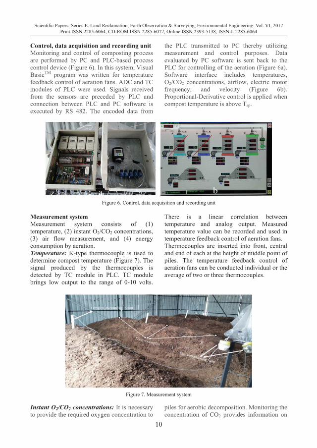
Control, data acquisition and recording unit Monitoring and control of composting process are performed by PC and PLC-based process control device (Figure 6). In this system, Visual BasicTM program was written for temperature feedback control of aeration fans. ADC and TC modules of PLC were used. Signals received from the sensors are preceded by PLC and connection between PLC and PC software is executed by RS 482. The encoded data from
the PLC transmitted to PC thereby utilizing measurement and control purposes. Data evaluated by PC software is sent back to the PLC for controlling of the aeration (Figure 6a). Software interface includes temperatures, O2/CO2 concentrations, airflow, electric motor frequency, and velocity (Figure 6b). Proportional-Derivative control is applied when compost temperature is above Tsp.
Figure 6. Control, data acquisition and recording unit
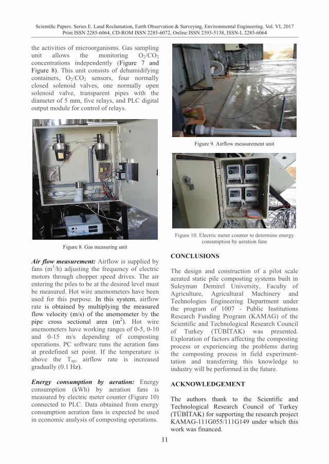
Measurement system Measurement system consists of (1) temperature, (2) instant O2/CO2 concentrations, (3) air flow measurement, and (4) energy consumption by aeration. Temperature: K-type thermocouple is used to determine compost temperature (Figure 7). The signal produced by the thermocouples is detected by TC module in PLC. TC module brings low output to the range of 0-10 volts.
There is a linear correlation between temperature and analog output. Measured temperature value can be recorded and used in temperature feedback control of aeration fans. Thermocouples are inserted into front, central and end of each at the height of middle point of piles. The temperature feedback control of aeration fans can be conducted individual or the average of two or three thermocouples.
Figure 7. Measurement system
Instant O2/CO2 concentrations: It is necessary to provide the required oxygen concentration to
piles for aerobic decomposition. Monitoring the concentration of CO2 provides information on
11
Scientific Papers. Series E. Land Reclamation, Earth Observation & Surveying, Environmental Engineering. Vol. VI, 2017Print ISSN 2285-6064, CD-ROM ISSN 2285-6072, Online ISSN 2393-5138, ISSN-L 2285-6064
Control, data acquisition and recording unit Monitoring and control of composting process are performed by PC and PLC-based process control device (Figure 6). In this system, Visual BasicTM program was written for temperature feedback control of aeration fans. ADC and TC modules of PLC were used. Signals received from the sensors are preceded by PLC and connection between PLC and PC software is executed by RS 482. The encoded data from
the PLC transmitted to PC thereby utilizing measurement and control purposes. Data evaluated by PC software is sent back to the PLC for controlling of the aeration (Figure 6a). Software interface includes temperatures, O2/CO2 concentrations, airflow, electric motor frequency, and velocity (Figure 6b). Proportional-Derivative control is applied when compost temperature is above Tsp.
Figure 6. Control, data acquisition and recording unit
Measurement system Measurement system consists of (1) temperature, (2) instant O2/CO2 concentrations, (3) air flow measurement, and (4) energy consumption by aeration. Temperature: K-type thermocouple is used to determine compost temperature (Figure 7). The signal produced by the thermocouples is detected by TC module in PLC. TC module brings low output to the range of 0-10 volts.
There is a linear correlation between temperature and analog output. Measured temperature value can be recorded and used in temperature feedback control of aeration fans. Thermocouples are inserted into front, central and end of each at the height of middle point of piles. The temperature feedback control of aeration fans can be conducted individual or the average of two or three thermocouples.
Figure 7. Measurement system
Instant O2/CO2 concentrations: It is necessary to provide the required oxygen concentration to
piles for aerobic decomposition. Monitoring the concentration of CO2 provides information on
the activities of microorganisms. Gas sampling unit allows the monitoring O2/CO2 concentrations independently (Figure 7 and Figure 8). This unit consists of dehumidifying containers, O2/CO2 sensors, four normally closed solenoid valves, one normally open solenoid valve, transparent pipes with the diameter of 5 mm, five relays, and PLC digital output module for control of relays.
Figure 8. Gas measuring unit
Air flow measurement: Airflow is supplied by fans (m3/h) adjusting the frequency of electric motors through chopper speed drives. The air entering the piles to be at the desired level must be measured. Hot wire anemometers have been used for this purpose. In this system, airflow rate is obtained by multiplying the measured flow velocity (m/s) of the anemometer by the pipe cross sectional area (m2). Hot wire anemometers have working ranges of 0-5, 0-10 and 0-15 m/s depending of composting operations. PC software runs the aeration fans at predefined set point. If the temperature is above the Tsp, airflow rate is increased gradually (0.1 Hz). Energy consumption by aeration: Energy consumption (kWh) by aeration fans is measured by electric meter counter (Figure 10) connected to PLC. Data obtained from energy consumption aeration fans is expected be used in economic analysis of composting operations.
Figure 9. Airflow measurement unit
Figure 10. Electric meter counter to determine energy
consumption by aeration fans CONCLUSIONS The design and construction of a pilot scale aerated static pile composting systems built in Suleyman Demirel University, Faculty of Agriculture, Agricultural Machinery and Technologies Engineering Department under the program of 1007 - Public Institutions Research Funding Program (KAMAG) of the Scientific and Technological Research Council of Turkey (TÜBİTAK) was presented. Exploration of factors affecting the composting process or experiencing the problems during the composting process in field experiment-tation and transferring this knowledge to industry will be performed in the future. ACKNOWLEDGEMENT The authors thank to the Scientific and Technological Research Council of Turkey (TÜBİTAK) for supporting the research project KAMAG-111G055/111G149 under which this work was financed.

12
Scientific Papers. Series E. Land Reclamation, Earth Observation & Surveying, Environmental Engineering. Vol. VI, 2017Print ISSN 2285-6064, CD-ROM ISSN 2285-6072, Online ISSN 2393-5138, ISSN-L 2285-6064
REFERENCES Keener, H.M., Dick, W.A., Hoitink, H.A.J., 2000.
Composting and beneficial utilization of composted by-product materials. In: Power, J.F., Dick, W.A., Kashmanian, R.M., Sims, J.T., Wright, R. J., Dawson, M. D., Bezdicek, D. (eds.), Beneficial Uses of Agricultural, Industrial and Municipal By-products. Soil Science Society of America. Madison, Wisconsin, 315-341.
Keener, H.M., M., Wicks, F.C. Michel, and Ekinci, K, 2014. Composting broiler litter. World's Poultry Science Journal, 70, 709-719.
Keener, H.M., Marugg, C., Hansen, R.C., Hoitink, H.A.J., 1993. Optimizing the efficiency of the composting process. In: Hoitink, H.A.J., Keener, H.M. (eds.), Science and Engineering of Composting: Design, Environmental, Microbiological and Utilization Aspects. Renaissance Publications, Ohio, 59-94.
Stentiford, E.I., 1996. Composting control: principles and practice. In: De Bertoldi, M., Sequi, P., Lemmes, B., Papi, T. (Eds), The Science of Composting. Blackie Academic & Professional, London, pp. 49-59.
13
Scientific Papers. Series E. Land Reclamation, Earth Observation & Surveying, Environmental Engineering. Vol. VI, 2017Print ISSN 2285-6064, CD-ROM ISSN 2285-6072, Online ISSN 2393-5138, ISSN-L 2285-6064
REFERENCES Keener, H.M., Dick, W.A., Hoitink, H.A.J., 2000.
Composting and beneficial utilization of composted by-product materials. In: Power, J.F., Dick, W.A., Kashmanian, R.M., Sims, J.T., Wright, R. J., Dawson, M. D., Bezdicek, D. (eds.), Beneficial Uses of Agricultural, Industrial and Municipal By-products. Soil Science Society of America. Madison, Wisconsin, 315-341.
Keener, H.M., M., Wicks, F.C. Michel, and Ekinci, K, 2014. Composting broiler litter. World's Poultry Science Journal, 70, 709-719.
Keener, H.M., Marugg, C., Hansen, R.C., Hoitink, H.A.J., 1993. Optimizing the efficiency of the composting process. In: Hoitink, H.A.J., Keener, H.M. (eds.), Science and Engineering of Composting: Design, Environmental, Microbiological and Utilization Aspects. Renaissance Publications, Ohio, 59-94.
Stentiford, E.I., 1996. Composting control: principles and practice. In: De Bertoldi, M., Sequi, P., Lemmes, B., Papi, T. (Eds), The Science of Composting. Blackie Academic & Professional, London, pp. 49-59.
ENVIRONMENTAL AND TECHNOLOGICAL ASPECTS OF USE OF RESIDUES FROM TOBACCO PRODUCTION AS HEATING FUEL
Dimitar KEHAYOV, Georgi KOMITOV
Agricultural University of Plovdiv, 12 Mendeleev Blvd., Plovdiv, Bulgaria
Corresponding author email: [email protected]
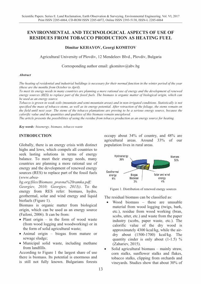
Abstract The heating of residential and industrial buildings is necessary for their normal function in the winter period of the year (these are the months from October to April). To meet its energy needs in many countries are planning a more rational use of energy and the development of renewed energy sources (RES) to replace part of the fossil fuels. The biomass is organic matter of biological origin, which can be used as an energy source. Tobacco is grown in weak soils (mountain and semi-mountain areas) and in non-irrigated conditions. Statistically is not specified the mass of tobacco stems, as well as its energy potential. After retraction of the foliage, the stems remain on the field until next year. The stems of the tobacco plantations are proving to be a serious energy source, because the calorific value and the quantities and qualities of this biomass remain unexplored. The article presents the possibilities of using the residue from tobacco production as an energy source for heating. Key words: bioenergy, biomass, tobacco waste INTRODUCTION Globally, there is an energy crisis with distinct highs and lows, which compels all countries to seek lasting solutions in terms of energy balance. To meet their energy needs, many countries are planning a more rational use of energy and the development of renewed energy sources (RES) to replace part of the fossil fuels (www.abea-bg.org/files/Biomass_pravna%20ramka.pdf; Georgiev, 2010; Georgiev, 2013)). To the energy from RES refer: biomass, hydro, geothermal, solar and wind energy and liquid biofuels (Figure 1). Biomass is organic matter from biological origin, which can be used as an energy source (Failoni, 2006). It can be from: � Plant origin – in the form of wood waste
(from wood logging and woodworking) or in the form of solid agricultural waste;
� Animal origin – biogas from mature or sewage sludge;
� Municipal solid waste, including methane from landfills.
According to Figure 1 the largest share of use there is biomass. Its potential is enormous and is still not fully known. Bulgarians forests
occupy about 34% of country, and 48% are agricultural areas. Around 33% of our population lives in rural areas.
Figure 1. Distribution of renewed energy sources
The residual biomass can be classified as: � Wood biomass – these are unusable
material from wood logging (twigs, bark, etc.), residue from wood working (bran, scobs, utter, etc.) and waste from the paper industry (scobs, paper waste, etc.). The calorific value of the dry wood is approximately 4300 kcal/kg, while the air-dry about (1500-1700) kcal/kg. The quantity cinder is only about (1-1.5) % (Zahariev, 2015).
� Solid agricultural biomass – mainly straw, corn stalks, sunflower stalks and flakes, tobacco stalks, clipping from orchards and vineyards. Studies show that about 30% of
14
Scientific Papers. Series E. Land Reclamation, Earth Observation & Surveying, Environmental Engineering. Vol. VI, 2017Print ISSN 2285-6064, CD-ROM ISSN 2285-6072, Online ISSN 2393-5138, ISSN-L 2285-6064
the straw quantity, 65% of the corn stalks and around 80% of the other solid agricultural biomass can be used for energy purposes (Al-Rifai, 2004; Georgiev, 2010).
Annual solid agricultural biomass is estimated at 800,000 t. Tobacco stems prove to be a serious energy source from agricultural biomass. Calorific value, quantities and qualities of this biomass remain unexplored and untapped - early spring under cultivation of fields, as cutting the remaining stems and leaving in the soil. WORKING METHODS To determine the quantity of residual biomass of unit area, arbitrarily converged 200 plants from proving ground, for each mass is determined. Measurement of the tobacco stalks mass is carried out with electronic scale "DENVER INSTRUMENT", model "PK202" with range up to 200 g and accuracy 0,01 g. After their reporting the received data are processed and determine the average mass of one wet plant. Next operation is drying of the stems into a stove to absolutely dry condition and weighted. The received results are processed and obtained the average value of mass from absolute dry plant. The humidity is determined by equation 1:
.100�
�M МF DWМB
% (1)
where: MF - average value for freshly harvested plant
mass, g; MD - the mass of absolutely dry plant, g. The quantity of biomass from tobacco stems at 1 ha is defined by equation 2:
.B FQ = i M [kg] (2) where: i - number of planted tobacco plants in 1 ha. Total residual biomass in the cultivation of small-leaved tobacco in Bulgaria for the year is derived from equation 3:
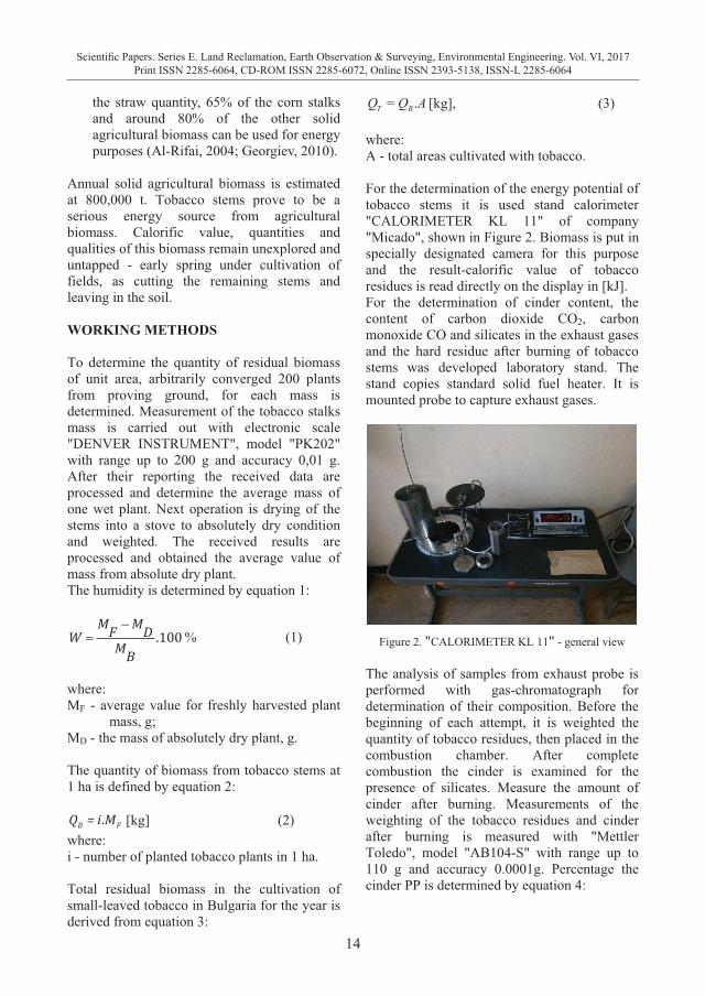
.T BQ = Q A [kg], (3) where: A - total areas cultivated with tobacco. For the determination of the energy potential of tobacco stems it is used stand calorimeter "CALORIMETER KL 11" of company "Micado", shown in Figure 2. Biomass is put in specially designated camera for this purpose and the result-calorific value of tobacco residues is read directly on the display in [kJ]. For the determination of cinder content, the content of carbon dioxide CO2, carbon monoxide CO and silicates in the exhaust gases and the hard residue after burning of tobacco stems was developed laboratory stand. The stand copies standard solid fuel heater. It is mounted probe to capture exhaust gases.
Figure 2. "CALORIMETER KL 11" - general view
The analysis of samples from exhaust probe is performed with gas-chromatograph for determination of their composition. Before the beginning of each attempt, it is weighted the quantity of tobacco residues, then placed in the combustion chamber. After complete combustion the cinder is examined for the presence of silicates. Measure the amount of cinder after burning. Measurements of the weighting of the tobacco residues and cinder after burning is measured with "Mettler Toledo", model "AB104-S" with range up to 110 g and accuracy 0.0001g. Percentage the cinder PP is determined by equation 4:
15
Scientific Papers. Series E. Land Reclamation, Earth Observation & Surveying, Environmental Engineering. Vol. VI, 2017Print ISSN 2285-6064, CD-ROM ISSN 2285-6072, Online ISSN 2393-5138, ISSN-L 2285-6064
the straw quantity, 65% of the corn stalks and around 80% of the other solid agricultural biomass can be used for energy purposes (Al-Rifai, 2004; Georgiev, 2010).
Annual solid agricultural biomass is estimated at 800,000 t. Tobacco stems prove to be a serious energy source from agricultural biomass. Calorific value, quantities and qualities of this biomass remain unexplored and untapped - early spring under cultivation of fields, as cutting the remaining stems and leaving in the soil. WORKING METHODS To determine the quantity of residual biomass of unit area, arbitrarily converged 200 plants from proving ground, for each mass is determined. Measurement of the tobacco stalks mass is carried out with electronic scale "DENVER INSTRUMENT", model "PK202" with range up to 200 g and accuracy 0,01 g. After their reporting the received data are processed and determine the average mass of one wet plant. Next operation is drying of the stems into a stove to absolutely dry condition and weighted. The received results are processed and obtained the average value of mass from absolute dry plant. The humidity is determined by equation 1:
.100�
�M МF DWМB
% (1)
where: MF - average value for freshly harvested plant
mass, g; MD - the mass of absolutely dry plant, g. The quantity of biomass from tobacco stems at 1 ha is defined by equation 2:
.B FQ = i M [kg] (2) where: i - number of planted tobacco plants in 1 ha. Total residual biomass in the cultivation of small-leaved tobacco in Bulgaria for the year is derived from equation 3:
.T BQ = Q A [kg], (3) where: A - total areas cultivated with tobacco. For the determination of the energy potential of tobacco stems it is used stand calorimeter "CALORIMETER KL 11" of company "Micado", shown in Figure 2. Biomass is put in specially designated camera for this purpose and the result-calorific value of tobacco residues is read directly on the display in [kJ]. For the determination of cinder content, the content of carbon dioxide CO2, carbon monoxide CO and silicates in the exhaust gases and the hard residue after burning of tobacco stems was developed laboratory stand. The stand copies standard solid fuel heater. It is mounted probe to capture exhaust gases.
Figure 2. "CALORIMETER KL 11" - general view
The analysis of samples from exhaust probe is performed with gas-chromatograph for determination of their composition. Before the beginning of each attempt, it is weighted the quantity of tobacco residues, then placed in the combustion chamber. After complete combustion the cinder is examined for the presence of silicates. Measure the amount of cinder after burning. Measurements of the weighting of the tobacco residues and cinder after burning is measured with "Mettler Toledo", model "AB104-S" with range up to 110 g and accuracy 0.0001g. Percentage the cinder PP is determined by equation 4:
.100� P
O
MPPM
(4)
where: MP - the mass of cinder, g; МО - mass of burnt tobacco residues, g. RESULTS AND DISCUSSIONS The average value of the mass from moist tobacco stem is 47.17 g, and at absolute dry state respectively is 25.4 g. Using dependence 1 humidity is obtained approximately 46%. The quantity of dry biomass from tobacco stems from 1 ha with according to dependence 2 and the results referred above is 304.8 kg in the 12,000 planted plants. Over the past (2-3) years small-leaved tobacco in Bulgaria is cultivated on around 138,000 ha. Using equation 3 for the total quantity of absolutely dry tobacco results approximately 42,000 t. The results of the experiments for the determination of the calorific value, cinder content, the presence of silicates in cinder, content of carbon monoxide and dioxide are listed in the table 1.
Table 1. Experimental results
Calorific value [kJ/kg] 18,332 Silicates [%] 2.94 Cinder content [%] 3.16 Content of СО2 [mg/m3] 3.24 Content of СО [mg/m3] 0.31 Energy [kWh/kg] 5.09 Calorific heat [kcal/kg] 4,378 It is seen that content of the cinder after the complete burning of tobacco stems is 3.16%. According to European certification EN-B this value must be less than 3.5% for pellets and between 0.3 and 6% for the chipped wood. In both cases, the obtained result meets to European requirements indicates that the tobacco waste is an appropriate power source. The presence of silicates in burning leads to deposits on the grids of the combustion chamber and reduce the air flow through them. In this case is disrupted the burning process. This can cause the halt of the combustion installation. This disadvantage is reduced using
removable grid, which are periodically washed with water. Content of the silicates in the hard waste after combustion of tobacco stems, is 2.94%. It is higher than that of certain solid wastes from agricultural production, such as sunflower -1.1% and lower than that of straw from wheat-up to 52%. For comparison, the rate of burning wood silicates is about 4.7%. In this study the contents of the silicates in the cinder allows burning of tobacco residues in standard heating systems. In terms of carbon dioxide and carbon monoxide there is no clear picture of the limit values. They depend both on the fuel that is used also by the device in which combustion takes place, working conditions, etc. The limit concentration of CO in the ambient air (which does not directly or indirectly affect, adversely affect the present and future generations, not lowers efficiency, not worse self-esteem and sanitary and household living conditions) is 3 mg/m3. From the data in the table 1 it is apparent that the burning of residues from tobacco plants it results that the quantity of units CO is much less than the permissible. The calorific value of the residues from agricultural production is less than that of the different types of wood with 20 to 30%. In some literary sources data show that straw, stalks of corn, vine sticks and oil cake have a calorific value 4,100 kcal/kg. This is equal of 4.77 kWh/kg energy. Studied by us tobacco residues is having energy 5.09 kWh/kg or 4,378 kcal/kg, which is comparable to the literature data. CONCLUSIONS The results of the four tracked indicators give grounds to assert that tobacco residues (stems, leaves and particles on them) may be used as heating fuel. Due to the contents of a small quantity of silicates in the cinder there is no danger from clogging the grids in the combustion chambers and suspension of the combustion process due to a lack of oxygen.

16
Scientific Papers. Series E. Land Reclamation, Earth Observation & Surveying, Environmental Engineering. Vol. VI, 2017Print ISSN 2285-6064, CD-ROM ISSN 2285-6072, Online ISSN 2393-5138, ISSN-L 2285-6064
REFERENCES Zahariev I.,Kehayov D., 2015. Results from research of
rose stems burning. University of Ruse Proceedings, vol. 54, book 1.1, Ruse, 123-125.
Failoni, 2006. Renewable energy sources. Trakia University, Stara Zagora.
www.abea-bg.org/files/Biomass_pravna%20ramka.pdf Al-Rifai, H., Y. Enakiev, B. Borisov, S. Mitev, 2004.
Research on practical opportunities for utilization of
plant lefts of the corn industry. EE&AE Proceeding 2004, Ruse, 658-665.
Georgiev, V., N. Markov, G. Kostadinov, L. Asenov, I. Ivanov, G. Kapashikov, Y. Enakiev, 2010. Fuel-technical specifications of straw from cereals. Agricultural Journal, vol. 1, Sofia, 32-35.
Georgiev, V., G. Kapashikov, L. Ivanov, I. Mortev, Y. Enakiev, 2013. Investigation of sunflower stems and heads combustion in chipped biomass combustion.
17
Scientific Papers. Series E. Land Reclamation, Earth Observation & Surveying, Environmental Engineering. Vol. VI, 2017Print ISSN 2285-6064, CD-ROM ISSN 2285-6072, Online ISSN 2393-5138, ISSN-L 2285-6064
REFERENCES Zahariev I.,Kehayov D., 2015. Results from research of
rose stems burning. University of Ruse Proceedings, vol. 54, book 1.1, Ruse, 123-125.
Failoni, 2006. Renewable energy sources. Trakia University, Stara Zagora.
www.abea-bg.org/files/Biomass_pravna%20ramka.pdf Al-Rifai, H., Y. Enakiev, B. Borisov, S. Mitev, 2004.
Research on practical opportunities for utilization of
plant lefts of the corn industry. EE&AE Proceeding 2004, Ruse, 658-665.
Georgiev, V., N. Markov, G. Kostadinov, L. Asenov, I. Ivanov, G. Kapashikov, Y. Enakiev, 2010. Fuel-technical specifications of straw from cereals. Agricultural Journal, vol. 1, Sofia, 32-35.
Georgiev, V., G. Kapashikov, L. Ivanov, I. Mortev, Y. Enakiev, 2013. Investigation of sunflower stems and heads combustion in chipped biomass combustion.
EVALUATING OF ELECTRIC ENERGY GENERATING POTENTIAL
USING BIOGAS FROM ANIMAL BIOMASSES IN BURDUR CITY
Recep KULCU, Cihannur CIHANALP
Suleyman Demirel University, Isparta, Turkey
Corresponding author email: [email protected] Abstract Today, with population increasing, industry growing up, technology advancing and getting involved with our lives ever so largely, the need for energy naturally increases. As current resources are failing to meet the requirements, search for alternative sources begins. Studies are rapidly increasing on a search for energy resources that are renewable, environment friendly, harmless to living beings and are not reliant on outside sources. Renewable energy resources are sustainable as they exist in the nature and do not have limited reserves. They also have strategic importance on the principle of sustainability as they do not produce greenhouse gas emissions upon usage. Today, renewable energy resources like the sun, wind, biomass, geothermal, hydraulics, hydrogen and wave energies are used in various ways, mainly for electricity. One of the renewable resources, biogas is a gas mixture emerging during oxygen-free fermentation of organic waste, and it is classified among biomass resources. In this study, we have determined the current animal quantity in Burdur city and calculated the amount of fertilizers obtained annually from these animals. Then the amounts of biogas, methane, electricity and thermal energy that can be produced out of these fertilizers is discovered should they be processed in biogas facilities. Figures show that based on 2015 statistics, 3.1mil tons of fertilizers is acquired annually from the animals in Burdur. Processing these fertilizers in biogas facilities can produce 79 million m3 of methane in a year. Burning this amount of methane in cogeneration systems can produce 275,740,415.72 kWh electricity and 315,131,903.68 kWh thermal energy annually. Key words: biogas, Burdur's potential of electric and thermal energy, renewable energy INTRODUCTION Developing technology, increasing population and growing economy demand an increase in the need for energy, resources as fossil fuels meeting these requirements are consumed ever so rapidly. The greenhouse gas emissions produced from using fossil fuels cause increase in world's average temperature, which results in serious environmental issues such as melting glaciers, disruption in rain regime, climate changes and warm streams changing directions. Beside from those problems, dependence in foreign resources caused more issues, and along with unstable prices, the last quarter of the century has naturally seen much more interest in renewable energy resources and their studies. Approximately 86% of the energy consumed around the world is supplied from fossil resources such as oil, natural gas and coal. Annual consumption rates of energy resources are as follows, 2015: 32.8% oil, 29.0% coal, 24.2% natural gas, 6.8% hydraulic, 4.5%
nuclear, 2.7% renewable (MENRa, 2016). These rates show that a large quantity of world's energy need is met by fossil energy resources. RENEWABLE ENERGY POTENTIAL OF TURKEY Growth of economy, population and technology increases the need for energy resources in Turkey, as it does for the rest of the world. Even though Turkey is advantageous in renewable resources for its geographical position, most of the energy need is supplied through fossil resources, most of which is imported from other countries. Ministry of Energy and Natural Resources in Turkey defines the country's energy policy as ''provision of energy resources in a manner to help economic growth and social projects and to accomplish this sufficiently, reliably and timely, considering economic and environ-mental conditions''. Over the increasing requests, the ministry 2015-2019 Strategic Plan
18
Scientific Papers. Series E. Land Reclamation, Earth Observation & Surveying, Environmental Engineering. Vol. VI, 2017Print ISSN 2285-6064, CD-ROM ISSN 2285-6072, Online ISSN 2393-5138, ISSN-L 2285-6064
consisting of 62 objectives on energy and natural resources (MENRb, 2016). Turkey's primary energy demand in the year 2014, equal to 123.9 million tons of oil (tpe) (867.3 million barrels) is distributed as: 32.50% natural gas, 29.20% coal, 28.50% oil, 6.70% renewable, 2.80% hydraulic and 0.30% others. Looking at the energy demand distribution on industries, 30% of the consumption is done in the circuit industry (producing electricity), 24% in housing and service, 23% in industry and 19% in transportation. Domestic supply rates of primary energy resources were figured as 25%, for the year of 2014. Imported energy supply rates have reached 75%, the highest point in the last ten years (MENRa, 2016). Values for 2016 are shown in Table 1.
Table 1. Electricty production in Turkey in 2016 distributed on resources (EA, 2016)
Production from Generation (mWh)
Rate (%)
Natural gas 85,678.193 32.97
Hydraulic 62,744.539 24.14
Imported Coal 43,945.821 16.91
Coal and Lignite 40,554.857 15.61
Wind 14,296.496 5.50
Geothermal 3,962.961 1.52
Other Thermal 2,265.807 0.87
Biogas 1,875.019 0.72
Imports 4,543.829 1.75
Of all the renewable energy resources, biomass energy holds significant importance. Biomass stands for organic forms based on plants and animals. Fuel production based on biomass is made by processing these forms. These processes include physical, chemical and biological practices. In processing biomass biologically to produce energy, the most common practice is biogas production. Biogas in Turkey Biogas is a colorless and flammable gas mixture that is produced through decomposing organic waste in an oxygen-free environment. In its main composition it consist of 60-70% methane (CH4), 30-40% carbon dioxide (CO2), 0-2% hydrogen sulfur (H2S), very little of nitrogen (N2) and hydrogen (H2).
Biogas usability for energy is based firstly upon the methane rate. Produced biogas is usually converted into electricity in thermal and energy stations (cogeneration) to be directly distributed in a local manner or electricity network. Table 2. Fundamental waste characteristics (BT, 2016).
Type of raw materials
Fertilizer per unit (kg/
animal/ day)
DS (%)
VDS (%)
Methane production/ raw material
(m3 CH4/ kg VDS)
Dairy Cattle 43 12 10 0.175 Beef Cattle 29 8.5 7.2 0.325 Calf 2.48 5.2 2.3 0.175 Pig 5.88 11 8.5 0.4 Sheep 2,4 11 9.2 0.3 Goat 2.05 13 9.5 0.3 Horse 20.4 15 10 0.3 Meat Chicken 0.187 22 17 0.35 Egg Hen 0.128 16 12 0.35 Turkey 0.376 12 9.1 0.35 Duck 0.33 31 19 0.35 Beetroot 18 79 0.46 Potato 25 79 0.28 Corn 85 72 0.41 Wheat 87 87 0.39 Rape 88 93 0.34 Grass 18 88 0.35 Clover 20 80 0.35 Pumpkin 22 82 0.26 Sugar Beet 15 80 0.23 Rye 85 87 0.37 Barley 93 86 0.44 Brewery 83 85 0.48 Slaughterhouse Wastewater 10 81 0.90
DS - Dry Substance; VDS - Volatile Dry Substance The thermal energy produced by burning the biogas can be used in heating the buildings and greenhouses nearby, drying hay, cooling milk or conditioning barns. For business profitability, it is crucial to benefit widely from both products (thermal energy and electricity). In Table 2, fertilizer production per animal unit, dry substance and volatile dry substance percentages and methane production per raw material are given based on each raw material. These parameters are used to get a hold on how much biogas and methane would be produced
19
Scientific Papers. Series E. Land Reclamation, Earth Observation & Surveying, Environmental Engineering. Vol. VI, 2017Print ISSN 2285-6064, CD-ROM ISSN 2285-6072, Online ISSN 2393-5138, ISSN-L 2285-6064
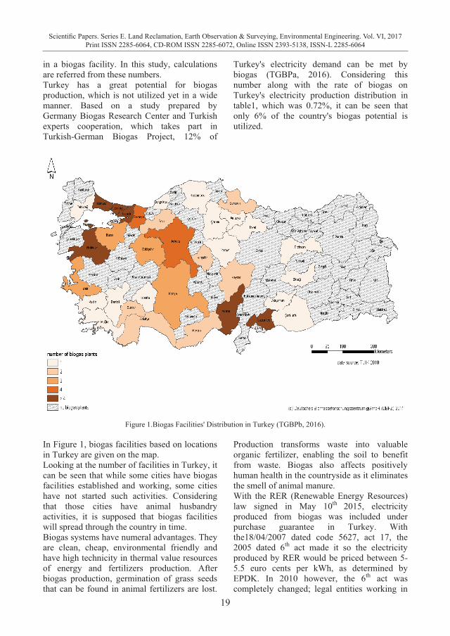
in a biogas facility. In this study, calculations are referred from these numbers. Turkey has a great potential for biogas production, which is not utilized yet in a wide manner. Based on a study prepared by Germany Biogas Research Center and Turkish experts cooperation, which takes part in Turkish-German Biogas Project, 12% of
Turkey's electricity demand can be met by biogas (TGBPa, 2016). Considering this number along with the rate of biogas on Turkey's electricity production distribution in table1, which was 0.72%, it can be seen that only 6% of the country's biogas potential is utilized.
Figure 1.Biogas Facilities' Distribution in Turkey (TGBPb, 2016).
In Figure 1, biogas facilities based on locations in Turkey are given on the map. Looking at the number of facilities in Turkey, it can be seen that while some cities have biogas facilities established and working, some cities have not started such activities. Considering that those cities have animal husbandry activities, it is supposed that biogas facilities will spread through the country in time. Biogas systems have numeral advantages. They are clean, cheap, environmental friendly and have high technicity in thermal value resources of energy and fertilizers production. After biogas production, germination of grass seeds that can be found in animal fertilizers are lost.
Production transforms waste into valuable organic fertilizer, enabling the soil to benefit from waste. Biogas also affects positively human health in the countryside as it eliminates the smell of animal manure. With the RER (Renewable Energy Resources) law signed in May 10th 2015, electricity produced from biogas was included under purchase guarantee in Turkey. With the18/04/2007 dated code 5627, act 17, the 2005 dated 6th act made it so the electricity produced by RER would be priced between 5-5.5 euro cents per kWh, as determined by EPDK. In 2010 however, the 6th act was completely changed; legal entities working in
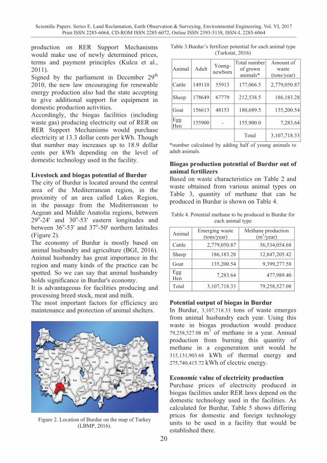
20
Scientific Papers. Series E. Land Reclamation, Earth Observation & Surveying, Environmental Engineering. Vol. VI, 2017Print ISSN 2285-6064, CD-ROM ISSN 2285-6072, Online ISSN 2393-5138, ISSN-L 2285-6064
production on RER Support Mechanisms would make use of newly determined prices, terms and payment principles (Kulcu et al., 2011). Signed by the parliament in December 29th 2010, the new law encouraging for renewable energy production also had the state accepting to give additional support for equipment in domestic production activities. Accordingly, the biogas facilities (including waste gas) producing electricity out of RER on RER Support Mechanisms would purchase electricity at 13.3 dollar cents per kWh. Though that number may increases up to 18.9 dollar cents per kWh depending on the level of domestic technology used in the facility. Livestock and biogas potential of Burdur The city of Burdur is located around the central area of the Mediterranean region, in the proximity of an area called Lakes Region, in the passage from the Mediterranean to Aegean and Middle Anatolia regions, between 29o-24' and 30o-53' eastern longitudes and between 36o-53' and 37o-50' northern latitudes (Figure 2). The economy of Burdur is mostly based on animal husbandry and agriculture (BGI, 2016). Animal husbandry has great importance in the region and many kinds of the practice can be spotted. So we can say that animal husbandry holds significance in Burdur's economy. It is advantageous for facilities producing and processing breed stock, meat and milk. The most important factors for efficiency are maintenance and protection of animal shelters.
Figure 2. Location of Burdur on the map of Turkey
(LBMP, 2016).
Table 3.Burdur’s fertilizer potential for each animal type (Turkstat, 2016)
Animal Adult Young-newborn
Total number of grown animals*
Amount of waste
(tons/year)
Cattle 149110 55913 177,066.5 2,779,050.87
Sheep 178649 67779 212,538.5 186,183.28
Goat 156613 48153 180,689.5 135,200.54
Egg Hen 155900 - 155,900.0 7,283.64
Total 3,107,718.33
*number calculated by adding half of young animals to adult animals. Biogas production potential of Burdur out of animal fertilizers Based on waste characteristics on Table 2 and waste obtained from various animal types on Table 3, quantity of methane that can be produced in Burdur is shown on Table 4.
Table 4. Potential methane to be produced in Burdur for
each animal type
Animal Emerging waste (tons/year)
Methane production (m3/year)
Cattle 2,779,050.87 56,534,054.68
Sheep 186,183.28 12,847,205.42
Goat 135,200.54 9,399,277.58 Egg Hen 7,283.64 477,989.40
Total 3,107,718.33 79,258,527.08
Potential output of biogas in Burdur In Burdur, 3,107,718.33 tons of waste emerges from animal husbandry each year. Using this waste in biogas production would produce 79,258,527.08 m3 of methane in a year. Annual production from burning this quantity of methane in a cogeneration unit would be 315,131,903.68 kWh of thermal energy and 275,740,415.72 kWh of electric energy. Economic value of electricity production Purchase prices of electricity produced in biogas facilities under RER laws depend on the domestic technology used in the facilities. As calculated for Burdur, Table 5 shows differing prices for domestic and foreign technology units to be used in a facility that would be established there.
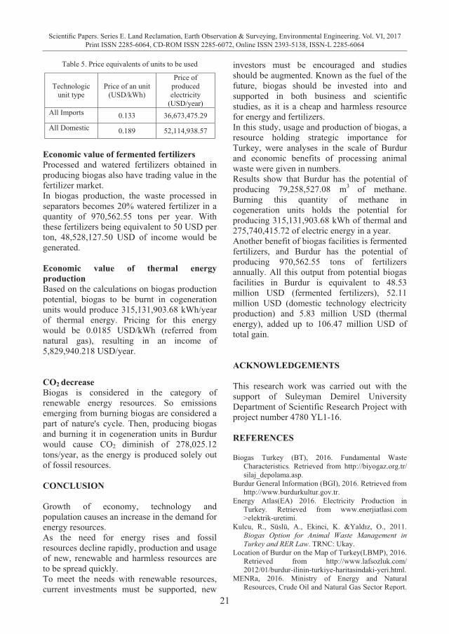
21
Scientific Papers. Series E. Land Reclamation, Earth Observation & Surveying, Environmental Engineering. Vol. VI, 2017Print ISSN 2285-6064, CD-ROM ISSN 2285-6072, Online ISSN 2393-5138, ISSN-L 2285-6064
production on RER Support Mechanisms would make use of newly determined prices, terms and payment principles (Kulcu et al., 2011). Signed by the parliament in December 29th 2010, the new law encouraging for renewable energy production also had the state accepting to give additional support for equipment in domestic production activities. Accordingly, the biogas facilities (including waste gas) producing electricity out of RER on RER Support Mechanisms would purchase electricity at 13.3 dollar cents per kWh. Though that number may increases up to 18.9 dollar cents per kWh depending on the level of domestic technology used in the facility. Livestock and biogas potential of Burdur The city of Burdur is located around the central area of the Mediterranean region, in the proximity of an area called Lakes Region, in the passage from the Mediterranean to Aegean and Middle Anatolia regions, between 29o-24' and 30o-53' eastern longitudes and between 36o-53' and 37o-50' northern latitudes (Figure 2). The economy of Burdur is mostly based on animal husbandry and agriculture (BGI, 2016). Animal husbandry has great importance in the region and many kinds of the practice can be spotted. So we can say that animal husbandry holds significance in Burdur's economy. It is advantageous for facilities producing and processing breed stock, meat and milk. The most important factors for efficiency are maintenance and protection of animal shelters.
Figure 2. Location of Burdur on the map of Turkey
(LBMP, 2016).
Table 3.Burdur’s fertilizer potential for each animal type (Turkstat, 2016)
Animal Adult Young-newborn
Total number of grown animals*
Amount of waste
(tons/year)
Cattle 149110 55913 177,066.5 2,779,050.87
Sheep 178649 67779 212,538.5 186,183.28
Goat 156613 48153 180,689.5 135,200.54
Egg Hen 155900 - 155,900.0 7,283.64
Total 3,107,718.33
*number calculated by adding half of young animals to adult animals. Biogas production potential of Burdur out of animal fertilizers Based on waste characteristics on Table 2 and waste obtained from various animal types on Table 3, quantity of methane that can be produced in Burdur is shown on Table 4.
Table 4. Potential methane to be produced in Burdur for
each animal type
Animal Emerging waste (tons/year)
Methane production (m3/year)
Cattle 2,779,050.87 56,534,054.68
Sheep 186,183.28 12,847,205.42
Goat 135,200.54 9,399,277.58 Egg Hen 7,283.64 477,989.40
Total 3,107,718.33 79,258,527.08
Potential output of biogas in Burdur In Burdur, 3,107,718.33 tons of waste emerges from animal husbandry each year. Using this waste in biogas production would produce 79,258,527.08 m3 of methane in a year. Annual production from burning this quantity of methane in a cogeneration unit would be 315,131,903.68 kWh of thermal energy and 275,740,415.72 kWh of electric energy. Economic value of electricity production Purchase prices of electricity produced in biogas facilities under RER laws depend on the domestic technology used in the facilities. As calculated for Burdur, Table 5 shows differing prices for domestic and foreign technology units to be used in a facility that would be established there.
Table 5. Price equivalents of units to be used
Technologic unit type
Price of an unit (USD/kWh)
Price of produced electricity
(USD/year) All Imports 0.133 36,673,475.29 All Domestic 0.189 52,114,938.57
Economic value of fermented fertilizers Processed and watered fertilizers obtained in producing biogas also have trading value in the fertilizer market. In biogas production, the waste processed in separators becomes 20% watered fertilizer in a quantity of 970,562.55 tons per year. With these fertilizers being equivalent to 50 USD per ton, 48,528,127.50 USD of income would be generated. Economic value of thermal energy production Based on the calculations on biogas production potential, biogas to be burnt in cogeneration units would produce 315,131,903.68 kWh/year of thermal energy. Pricing for this energy would be 0.0185 USD/kWh (referred from natural gas), resulting in an income of 5,829,940.218 USD/year. CO2 decrease Biogas is considered in the category of renewable energy resources. So emissions emerging from burning biogas are considered a part of nature's cycle. Then, producing biogas and burning it in cogeneration units in Burdur would cause CO2 diminish of 278,025.12 tons/year, as the energy is produced solely out of fossil resources. CONCLUSION Growth of economy, technology and population causes an increase in the demand for energy resources. As the need for energy rises and fossil resources decline rapidly, production and usage of new, renewable and harmless resources are to be spread quickly. To meet the needs with renewable resources, current investments must be supported, new
investors must be encouraged and studies should be augmented. Known as the fuel of the future, biogas should be invested into and supported in both business and scientific studies, as it is a cheap and harmless resource for energy and fertilizers. In this study, usage and production of biogas, a resource holding strategic importance for Turkey, were analyses in the scale of Burdur and economic benefits of processing animal waste were given in numbers. Results show that Burdur has the potential of producing 79,258,527.08 m3 of methane. Burning this quantity of methane in cogeneration units holds the potential for producing 315,131,903.68 kWh of thermal and 275,740,415.72 of electric energy in a year. Another benefit of biogas facilities is fermented fertilizers, and Burdur has the potential of producing 970,562.55 tons of fertilizers annually. All this output from potential biogas facilities in Burdur is equivalent to 48.53 million USD (fermented fertilizers), 52.11 million USD (domestic technology electricity production) and 5.83 million USD (thermal energy), added up to 106.47 million USD of total gain. ACKNOWLEDGEMENTS This research work was carried out with the support of Suleyman Demirel University Department of Scientific Research Project with project number 4780 YL1-16. REFERENCES Biogas Turkey (BT), 2016. Fundamental Waste
Characteristics. Retrieved from http://biyogaz.org.tr/ silaj_depolama.asp.
Burdur General Information (BGI), 2016. Retrieved from http://www.burdurkultur.gov.tr.
Energy Atlas(EA) 2016. Electricity Production in Turkey. Retrieved from www.enerjiatlasi.com >elektrik-uretimi.
Kulcu, R., Süslü, A., Ekinci, K. &Yaldız, O., 2011. Biogas Option for Animal Waste Management in Turkey and RER Law. TRNC: Ukay.
Location of Burdur on the Map of Turkey(LBMP), 2016. Retrieved from http://www.lafsozluk.com/ 2012/01/burdur-ilinin-turkiye-haritasindaki-yeri.html.
MENRa, 2016. Ministry of Energy and Natural Resources, Crude Oil and Natural Gas Sector Report.

22
Scientific Papers. Series E. Land Reclamation, Earth Observation & Surveying, Environmental Engineering. Vol. VI, 2017Print ISSN 2285-6064, CD-ROM ISSN 2285-6072, Online ISSN 2393-5138, ISSN-L 2285-6064
Retrieved from www.enerji.gov.tr>File> TP_HAM_PLTROL
MENRb. 2016. Ministry of Energy and Natural Resources. 2015-2019 Strategic Plan. Retrieved from www.sp.enerji.gov.tr/ETKB_2015_2019_Stratejik_Plani.
Turkish-German Biogas Project (TGBPa), 2016. What is Biogas? Retrieved from www.biyogaz.web.tr/ tr/biyogaz-nedir.
Turkish-German Biogas Project (TGBPb), 2016. Biogas Potential Report of Turkey. Retrieved from http://www.biyogaz.web.tr>files>docs. TurkStat, 2016. Database. Retrieved from https://biruni.tuik.gov.tr/hayvancilikapp/hayvancilik.zul.
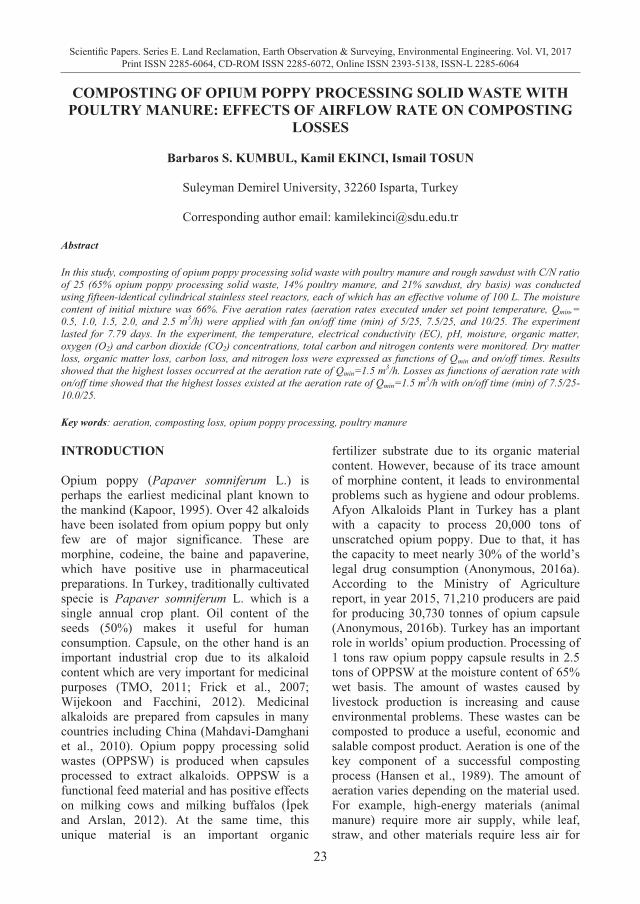
23
Scientific Papers. Series E. Land Reclamation, Earth Observation & Surveying, Environmental Engineering. Vol. VI, 2017Print ISSN 2285-6064, CD-ROM ISSN 2285-6072, Online ISSN 2393-5138, ISSN-L 2285-6064
Retrieved from www.enerji.gov.tr>File> TP_HAM_PLTROL
MENRb. 2016. Ministry of Energy and Natural Resources. 2015-2019 Strategic Plan. Retrieved from www.sp.enerji.gov.tr/ETKB_2015_2019_Stratejik_Plani.
Turkish-German Biogas Project (TGBPa), 2016. What is Biogas? Retrieved from www.biyogaz.web.tr/ tr/biyogaz-nedir.
Turkish-German Biogas Project (TGBPb), 2016. Biogas Potential Report of Turkey. Retrieved from http://www.biyogaz.web.tr>files>docs. TurkStat, 2016. Database. Retrieved from https://biruni.tuik.gov.tr/hayvancilikapp/hayvancilik.zul.
COMPOSTING OF OPIUM POPPY PROCESSING SOLID WASTE WITH
POULTRY MANURE: EFFECTS OF AIRFLOW RATE ON COMPOSTING LOSSES
Barbaros S. KUMBUL, Kamil EKINCI, Ismail TOSUN
Suleyman Demirel University, 32260 Isparta, Turkey
Corresponding author email: [email protected]
Abstract In this study, composting of opium poppy processing solid waste with poultry manure and rough sawdust with C/N ratio of 25 (65% opium poppy processing solid waste, 14% poultry manure, and 21% sawdust, dry basis) was conducted using fifteen-identical cylindrical stainless steel reactors, each of which has an effective volume of 100 L. The moisture content of initial mixture was 66%. Five aeration rates (aeration rates executed under set point temperature, Qmin,= 0.5, 1.0, 1.5, 2.0, and 2.5 m3/h) were applied with fan on/off time (min) of 5/25, 7.5/25, and 10/25. The experiment lasted for 7.79 days. In the experiment, the temperature, electrical conductivity (EC), pH, moisture, organic matter, oxygen (O2) and carbon dioxide (CO2) concentrations, total carbon and nitrogen contents were monitored. Dry matter loss, organic matter loss, carbon loss, and nitrogen loss were expressed as functions of Qmin and on/off times. Results showed that the highest losses occurred at the aeration rate of Qmin=1.5 m3/h. Losses as functions of aeration rate with on/off time showed that the highest losses existed at the aeration rate of Qmin=1.5 m3/h with on/off time (min) of 7.5/25-10.0/25. Key words: aeration, composting loss, opium poppy processing, poultry manure INTRODUCTION Opium poppy (Papaver somniferum L.) is perhaps the earliest medicinal plant known to the mankind (Kapoor, 1995). Over 42 alkaloids have been isolated from opium poppy but only few are of major significance. These are morphine, codeine, the baine and papaverine, which have positive use in pharmaceutical preparations. In Turkey, traditionally cultivated specie is Papaver somniferum L. which is a single annual crop plant. Oil content of the seeds (50%) makes it useful for human consumption. Capsule, on the other hand is an important industrial crop due to its alkaloid content which are very important for medicinal purposes (TMO, 2011; Frick et al., 2007; Wijekoon and Facchini, 2012). Medicinal alkaloids are prepared from capsules in many countries including China (Mahdavi-Damghani et al., 2010). Opium poppy processing solid wastes (OPPSW) is produced when capsules processed to extract alkaloids. OPPSW is a functional feed material and has positive effects on milking cows and milking buffalos (İpek and Arslan, 2012). At the same time, this unique material is an important organic
fertilizer substrate due to its organic material content. However, because of its trace amount of morphine content, it leads to environmental problems such as hygiene and odour problems. Afyon Alkaloids Plant in Turkey has a plant with a capacity to process 20,000 tons of unscratched opium poppy. Due to that, it has the capacity to meet nearly 30% of the world’s legal drug consumption (Anonymous, 2016a). According to the Ministry of Agriculture report, in year 2015, 71,210 producers are paid for producing 30,730 tonnes of opium capsule (Anonymous, 2016b). Turkey has an important role in worlds’ opium production. Processing of 1 tons raw opium poppy capsule results in 2.5 tons of OPPSW at the moisture content of 65% wet basis. The amount of wastes caused by livestock production is increasing and cause environmental problems. These wastes can be composted to produce a useful, economic and salable compost product. Aeration is one of the key component of a successful composting process (Hansen et al., 1989). The amount of aeration varies depending on the material used. For example, high-energy materials (animal manure) require more air supply, while leaf, straw, and other materials require less air for
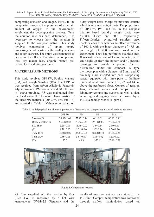
24
Scientific Papers. Series E. Land Reclamation, Earth Observation & Surveying, Environmental Engineering. Vol. VI, 2017Print ISSN 2285-6064, CD-ROM ISSN 2285-6072, Online ISSN 2393-5138, ISSN-L 2285-6064
composting (Finstein and Hogan, 1993). In the composting process, the presence of a certain amount of oxygen in the environment accelerates the decomposition process. Once the aeration rate has been determined, it is necessary to choose how the aeration is supplied to the compost matrix. This study involves composting of opium poppy processing solid wastes with poultry manure and rough sawdust. The study was conducted to determine the effects of aeration on composting loss (dry matter loss, organic matter loss, carbon loss, and nitrogen loss). MATERIALS AND METHODS This study involved OPPSW, Poultry Manure (PM) and Rough Sawdust (RS). The OPPSW was received from Afyon Alkaloids Factoryin Afyon province. PM was received Gürelli farm in Isparta province. RS was maintained from the local sawmill. The main characteristics of the three raw materials (OPPSW, PM, and RS) are reported in Table 1. Values reported are on
a dry weight basis except for moisture content which is on a wet weight basis. The proportions of OPPSW, PM, and RS in the compost mixture based on dry weight basis were 65.38%, 13.99, and 20.63, respectively. Fifteen-identical cylindrical stainless steel reactors, each of which has an effective volume of 100 L with the inner diameter of 47.3 cm and height of 57.0 cm were used in the experiment. They had perforated stainless steel floors with a hole size of 4 mm (diameter) at 13 cm height up from the bottom and 40 percent openings to provide a plenum for air distribution under the compost. K type thermocouples with a diameter of 3 mm and 35 cm length are inserted into each composting reactor equipped with three ports to facilitate temperature at three levels of 10, 27, and 44 cm above the perforated floor. Control of aeration fans, solenoid valves and pumps in the laboratory composting systems as well as data acquiring and logging were performed by a PLC (Schneider M258) (Figure 1).
Table 1. Initial physical and chemical properties of feedstock and composting mix used in the experiment
OPPSW PM RS Mix Moisture,% 35.52±1.60 72.42±0.44 6.1±0.01 66.10±0.86 Organic matter, % 55.39±0.27 70.52±0.31 99.18±0.05 76.00±0.81 EC, dS/m 2.21±0.01 11.48±0.02 3.9±0.14 2.99±0.15 pH 8.78±0.05 5.22±0.00 5.7±0.14 8.70±0.10 Total C, % 33.00±0.05 35.41±0.08 48.60±0.10 38.04±0.24 Total N, % 0.88±0.06 5.87±0.03 0.13±0.02 1.52±0.02 C/N 37.5 6.03 373.85 25.11±0.51
Figure 1. Composting reactors
Air flow supplied into the reactors by fans (0.25 kW) is measured by a hot wire anemometer (QVM62.1 Siemens) and the
results of measurement are transmitted to the PLC unit. Compost temperature was controlled through airflow manipulation based on
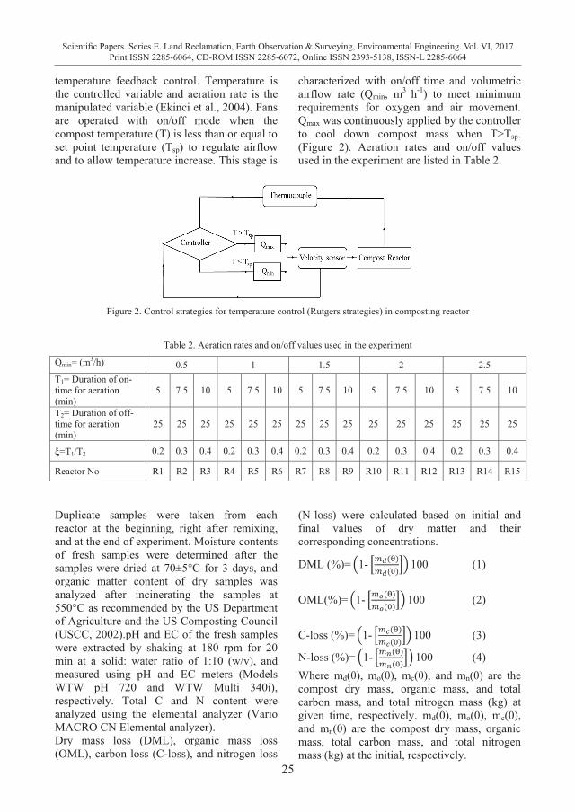
25
Scientific Papers. Series E. Land Reclamation, Earth Observation & Surveying, Environmental Engineering. Vol. VI, 2017Print ISSN 2285-6064, CD-ROM ISSN 2285-6072, Online ISSN 2393-5138, ISSN-L 2285-6064
composting (Finstein and Hogan, 1993). In the composting process, the presence of a certain amount of oxygen in the environment accelerates the decomposition process. Once the aeration rate has been determined, it is necessary to choose how the aeration is supplied to the compost matrix. This study involves composting of opium poppy processing solid wastes with poultry manure and rough sawdust. The study was conducted to determine the effects of aeration on composting loss (dry matter loss, organic matter loss, carbon loss, and nitrogen loss). MATERIALS AND METHODS This study involved OPPSW, Poultry Manure (PM) and Rough Sawdust (RS). The OPPSW was received from Afyon Alkaloids Factoryin Afyon province. PM was received Gürelli farm in Isparta province. RS was maintained from the local sawmill. The main characteristics of the three raw materials (OPPSW, PM, and RS) are reported in Table 1. Values reported are on
a dry weight basis except for moisture content which is on a wet weight basis. The proportions of OPPSW, PM, and RS in the compost mixture based on dry weight basis were 65.38%, 13.99, and 20.63, respectively. Fifteen-identical cylindrical stainless steel reactors, each of which has an effective volume of 100 L with the inner diameter of 47.3 cm and height of 57.0 cm were used in the experiment. They had perforated stainless steel floors with a hole size of 4 mm (diameter) at 13 cm height up from the bottom and 40 percent openings to provide a plenum for air distribution under the compost. K type thermocouples with a diameter of 3 mm and 35 cm length are inserted into each composting reactor equipped with three ports to facilitate temperature at three levels of 10, 27, and 44 cm above the perforated floor. Control of aeration fans, solenoid valves and pumps in the laboratory composting systems as well as data acquiring and logging were performed by a PLC (Schneider M258) (Figure 1).
Table 1. Initial physical and chemical properties of feedstock and composting mix used in the experiment
OPPSW PM RS Mix Moisture,% 35.52±1.60 72.42±0.44 6.1±0.01 66.10±0.86 Organic matter, % 55.39±0.27 70.52±0.31 99.18±0.05 76.00±0.81 EC, dS/m 2.21±0.01 11.48±0.02 3.9±0.14 2.99±0.15 pH 8.78±0.05 5.22±0.00 5.7±0.14 8.70±0.10 Total C, % 33.00±0.05 35.41±0.08 48.60±0.10 38.04±0.24 Total N, % 0.88±0.06 5.87±0.03 0.13±0.02 1.52±0.02 C/N 37.5 6.03 373.85 25.11±0.51
Figure 1. Composting reactors
Air flow supplied into the reactors by fans (0.25 kW) is measured by a hot wire anemometer (QVM62.1 Siemens) and the
results of measurement are transmitted to the PLC unit. Compost temperature was controlled through airflow manipulation based on
temperature feedback control. Temperature is the controlled variable and aeration rate is the manipulated variable (Ekinci et al., 2004). Fans are operated with on/off mode when the compost temperature (T) is less than or equal to set point temperature (Tsp) to regulate airflow and to allow temperature increase. This stage is
characterized with on/off time and volumetric airflow rate (Qmin, m3 h-1) to meet minimum requirements for oxygen and air movement. Qmax was continuously applied by the controller to cool down compost mass when T>Tsp. (Figure 2). Aeration rates and on/off values used in the experiment are listed in Table 2.
Figure 2. Control strategies for temperature control (Rutgers strategies) in composting reactor
Table 2. Aeration rates and on/off values used in the experiment
Qmin= (m3/h) 0.5 1 1.5 2 2.5 T1= Duration of on- time for aeration (min)
5 7.5 10 5 7.5 10 5 7.5 10 5 7.5 10 5 7.5 10
T2= Duration of off-time for aeration (min)
25 25 25 25 25 25 25 25 25 25 25 25 25 25 25
�=T1/T2 0.2 0.3 0.4 0.2 0.3 0.4 0.2 0.3 0.4 0.2 0.3 0.4 0.2 0.3 0.4
Reactor No R1 R2 R3 R4 R5 R6 R7 R8 R9 R10 R11 R12 R13 R14 R15
Duplicate samples were taken from each reactor at the beginning, right after remixing, and at the end of experiment. Moisture contents of fresh samples were determined after the samples were dried at 70±5°C for 3 days, and organic matter content of dry samples was analyzed after incinerating the samples at 550°C as recommended by the US Department of Agriculture and the US Composting Council (USCC, 2002).pH and EC of the fresh samples were extracted by shaking at 180 rpm for 20 min at a solid: water ratio of 1:10 (w/v), and measured using pH and EC meters (Models WTW pH 720 and WTW Multi 340i), respectively. Total C and N content were analyzed using the elemental analyzer (Vario MACRO CN Elemental analyzer). Dry mass loss (DML), organic mass loss (OML), carbon loss (C-loss), and nitrogen loss
(N-loss) were calculated based on initial and final values of dry matter and their corresponding concentrations.
DML (%)= 1- 100 (1) OML(%)= 1- 100 (2) C-loss (%)= 1- 100 (3)
N-loss (%)= 1- 100 (4) Where md(θ), mo(θ), mc(θ), and mn(θ) are the compost dry mass, organic mass, and total carbon mass, and total nitrogen mass (kg) at given time, respectively. md(0), mo(0), mc(0), and mn(0) are the compost dry mass, organic mass, total carbon mass, and total nitrogen mass (kg) at the initial, respectively.
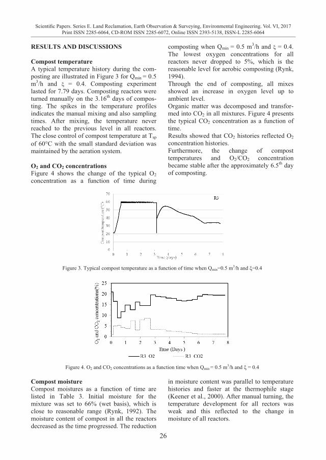
26
Scientific Papers. Series E. Land Reclamation, Earth Observation & Surveying, Environmental Engineering. Vol. VI, 2017Print ISSN 2285-6064, CD-ROM ISSN 2285-6072, Online ISSN 2393-5138, ISSN-L 2285-6064
RESULTS AND DISCUSSIONS Compost temperature A typical temperature history during the com-posting are illustrated in Figure 3 for Qmin = 0.5 m3/h and � = 0.4. Composting experiment lasted for 7.79 days. Composting reactors were turned manually on the 3.16th days of compos-ting. The spikes in the temperature profiles indicates the manual mixing and also sampling times. After mixing, the temperature never reached to the previous level in all reactors. The close control of compost temperature at Tsp
of 60�C with the small standard deviation was maintained by the aeration system. O2 and CO2 concentrations Figure 4 shows the change of the typical O2 concentration as a function of time during
composting when Qmin = 0.5 m3/h and � = 0.4. The lowest oxygen concentrations for all reactors never dropped to 5%, which is the reasonable level for aerobic composting (Rynk, 1994). Through the end of composting, all mixes showed an increase in oxygen level up to ambient level.Organic matter was decomposed and transfor-med into CO2 in all mixtures. Figure 4 presents the typical CO2 concentration as a function of time. Results showed that CO2 histories reflected O2concentration histories. Furthermore, the change of compost temperatures and O2/CO2 concentration became stable after the approximately 6.5th day of composting.
Figure 3. Typical compost temperature as a function of time when Qmin=0.5 m3/h and �=0.4
Figure 4. O2 and CO2 concentrations as a function time when Qmin = 0.5 m3/h and � = 0.4
Compost moisture Compost moistures as a function of time are listed in Table 3. Initial moisture for the mixture was set to 66% (wet basis), which is close to reasonable range (Rynk, 1992). The moisture content of compost in all the reactors decreased as the time progressed. The reduction
in moisture content was parallel to temperature histories and faster at the thermophile stage (Keener et al., 2000). After manual turning, the temperature development for all rectors was weak and this reflected to the change in moisture of all reactors.
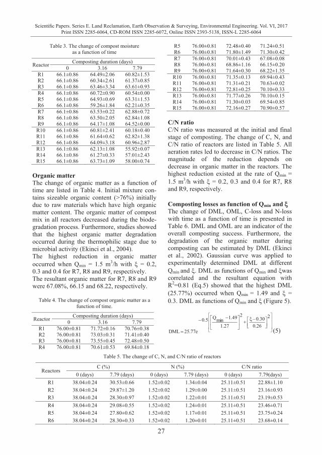
27
Scientific Papers. Series E. Land Reclamation, Earth Observation & Surveying, Environmental Engineering. Vol. VI, 2017Print ISSN 2285-6064, CD-ROM ISSN 2285-6072, Online ISSN 2393-5138, ISSN-L 2285-6064
Table 3. The change of compost moisture as a function of time
Reactor Composting duration (days) 0 3.16 7.79
R1 66.1±0.86 64.49±2.06 60.82±1.53 R2 66.1±0.86 60.34±2.61 61.37±0.85 R3 66.1±0.86 63.46±3.34 63.61±0.93 R4 66.1±0.86 60.72±0.90 60.54±0.00 R5 66.1±0.86 64.93±0.69 63.31±1.53 R6 66.1±0.86 59.26±1.84 62.21±0.35 R7 66.1±0.86 63.53±0.22 62.88±0.72 R8 66.1±0.86 63.50±2.05 62.84±1.08 R9 66.1±0.86 64.17±1.08 64.52±0.00
R10 66.1±0.86 60.81±2.41 60.18±0.40 R11 66.1±0.86 61.64±0.62 62.82±1.38 R12 66.1±0.86 64.09±3.18 60.96±2.87 R13 66.1±0.86 62.13±1.08 55.92±0.07 R14 66.1±0.86 61.27±0.33 57.01±2.43 R15 66.1±0.86 63.73±1.09 58.00±0.74
Organic matter The change of organic matter as a function of time are listed in Table 4. Initial mixture con-tains sizeable organic content (>76%) initially due to raw materials which have high organic matter content. The organic matter of compost mix in all reactors decreased during the biode-gradation process. Furthermore, studies showed that the highest organic matter degradation occurred during the thermophilic stage due to microbial activity (Ekinci et al., 2004). The highest reduction in organic matter occurred when Qmin = 1.5 m3/h with � = 0.2, 0.3 and 0.4 for R7, R8 and R9, respectively. The resultant organic matter for R7, R8 and R9 were 67.08%, 66.15 and 68.22, respectively.
Table 4. The change of compost organic matter as a function of time.
Reactor Composting duration (days) 0 3.16 7.79
R1 76.00±0.81 71.72±0.16 70.76±0.38 R2 76.00±0.81 73.03±0.31 71.41±0.40 R3 76.00±0.81 73.55±0.45 72.48±0.50 R4 76.00±0.81 70.61±0.53 69.84±0.18
R5 76.00±0.81 72.48±0.40 71.24±0.51 R6 76.00±0.81 71.80±1.49 71.30±0.42 R7 76.00±0.81 70.01±0.43 67.08±0.08 R8 76.00±0.81 68.86±1.16 66.15±0.20 R9 76.00±0.81 71.64±0.30 68.22±1.35
R10 76.00±0.81 71.35±0.13 69.94±0.43 R11 76.00±0.81 71.31±0.21 70.63±0.02 R12 76.00±0.81 72.81±0.25 70.10±0.33 R13 76.00±0.81 71.77±0.26 70.10±0.15 R14 76.00±0.81 71.30±0.03 69.54±0.85 R15 76.00±0.81 72.16±0.27 70.90±0.57
C/N ratio C/N ratio was measured at the initial and final stage of composting. The change of C, N, and C/N ratio of reactors are listed in Table 5. All aeration rates led to decrease in C/N ratios. The magnitude of the reduction depends on decrease in organic matter in the reactors. The highest reduction existed at the rate of Qmin = 1.5 m3/h with � = 0.2, 0.3 and 0.4 for R7, R8 and R9, respectively. Composting losses as function of Qmin and � The change of DML, OML, C-loss and N-loss with time as a function of time is presented in Table 6. DML and OML are an indicator of the overall composting success. Furthermore, the degradation of the organic matter during composting can be estimated by DML (Ekinci et al., 2002). Gaussian curve was applied to experimentally determined DML at different Qmin and �. DML as functions of Qmin and �was correlated and the resultant equation with R2=0.81 (Eq.5) showed that the highest DML (25.77%) occurred when Qmin = 1.49 and � = 0.3. DML as functions of Qmin and � (Figure 5).
���
�
�
���
�
�
���
��� ����
�
���
� ��
�
2
26.030.0
2
27.149.1minQ5.0
e77.25DML (5)
Table 5. The change of C, N, and C/N ratio of reactors
Reactors C (%) N (%) C/N ratio
0 (days) 7.79 (days) 0 (days) 7.79 (days) 0 (days) 7.79(days) R1 38.04±0.24 30.53±0.66 1.52±0.02 1.34±0.04 25.11±0.51 22.88±1.10 R2 38.04±0.24 29.87±1.20 1.52±0.02 1.29±0.00 25.11±0.51 23.16±0.93 R3 38.04±0.24 28.30±0.97 1.52±0.02 1.22±0.01 25.11±0.51 23.19±0.53 R4 38.04±0.24 29.08±0.55 1.52±0.02 1.24±0.01 25.11±0.51 23.46±0.71 R5 38.04±0.24 27.80±0.62 1.52±0.02 1.17±0.01 25.11±0.51 23.75±0.24 R6 38.04±0.24 28.30±0.33 1.52±0.02 1.20±0.01 25.11±0.51 23.68±0.14
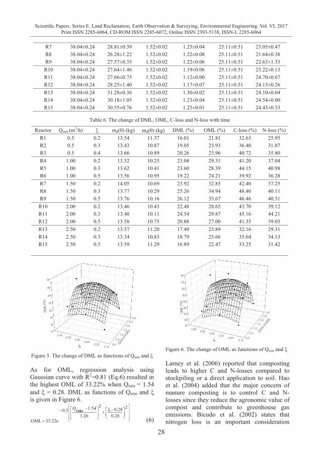
28
Scientific Papers. Series E. Land Reclamation, Earth Observation & Surveying, Environmental Engineering. Vol. VI, 2017Print ISSN 2285-6064, CD-ROM ISSN 2285-6072, Online ISSN 2393-5138, ISSN-L 2285-6064
R7 38.04±0.24 28.81±0.39 1.52±0.02 1.25±0.04 25.11±0.51 23.05±0.47 R8 38.04±0.24 26.28±1.22 1.52±0.02 1.22±0.08 25.11±0.51 21.64±0.38 R9 38.04±0.24 27.57±0.35 1.52±0.02 1.22±0.06 25.11±0.51 22.63±1.33
R10 38.04±0.24 27.64±1.46 1.52±0.02 1.19±0.06 25.11±0.51 23.22±0.13 R11 38.04±0.24 27.66±0.75 1.52±0.02 1.12±0.00 25.11±0.51 24.70±0.67 R12 38.04±0.24 28.25±1.40 1.52±0.02 1.17±0.07 25.11±0.51 24.15±0.26 R13 38.04±0.24 31.28±0.36 1.52±0.02 1.30±0.02 25.11±0.51 24.10±0.04 R14 38.04±0.24 30.18±1.05 1.52±0.02 1.23±0.04 25.11±0.51 24.54±0.00 R15 38.04±0.24 30.55±0.76 1.52±0.02 1.25±0.01 25.11±0.51 24.43±0.33
Table 6. The change of DML, OML, C-loss and N-loss with time
Reactor Qmin (m3/h) � md(0) (kg) md(�) (kg) DML (%) OML (%) C-loss (%) N-loss (%) R1 0.5 0.2 13.54 11.37 16.01 21.81 32.63 25.95 R2 0.5 0.3 13.43 10.87 19.05 23.93 36.40 31.07 R3 0.5 0.4 13.66 10.89 20.26 23.96 40.72 35.80 R4 1.00 0.2 13.32 10.25 23.08 29.31 41.20 37.04 R5 1.00 0.3 13.62 10.41 23.60 28.39 44.15 40.98 R6 1.00 0.5 13.56 10.95 19.22 24.21 39.92 36.28 R7 1.50 0.2 14.05 10.69 23.92 32.85 42.40 37.25 R8 1.50 0.3 13.77 10.29 25.26 34.94 48.40 40.11 R9 1.50 0.5 13.76 10.16 26.12 33.67 46.46 40.51
R10 2.00 0.2 13.46 10.43 22.48 28.65 43.70 39.12 R11 2.00 0.3 13.40 10.11 24.54 29.87 45.16 44.21 R12 2.00 0.5 13.58 10.75 20.88 27.00 41.35 39.03 R13 2.50 0.2 13.57 11.20 17.49 23.89 32.16 29.31 R14 2.50 0.3 13.34 10.83 18.79 25.66 35.64 34.13 R15 2.50 0.5 13.59 11.29 16.89 22.47 33.25 31.42
14
16
18
20
22
24
26
28
0.0
0.51.0
1.52.0
2.53.0
0.150.20
0.250.30
0.350.40
DM
L (%
)
Qmin (m
3/h)
Figure 5. The change of DML as functions of Qmin and � As for OML, regression analysis using Gaussian curve with R2=0.81 (Eq.6) resulted in the highest OML of 33.22% when Qmin = 1.54 and � = 0.28. DML as functions of Qmin and � is given in Figure 6.
���
�
�
���
�
�
���
��� ����
�
���
� ��
�
2
28.028.0
2
26.154.1minQ5.0
e22.33OML (6)
20
22
24
26
28
30
32
34
36
0.00.5
1.01.5
2.02.5
3.0
0.150.20
0.250.30
0.350.40
OM
L (%
)
Qmin (m
3/h)
Figure 6. The change of OML as functions of Qmin and � Larney et al. (2006) reported that composting leads to higher C and N-losses compared to stockpiling or a direct application to soil. Hao et al. (2004) added that the major concern of manure composting is to control C and N-losses since they reduce the agronomic value of compost and contribute to greenhouse gas emissions. Bicudo et al. (2002) states that nitrogen loss is an important consideration
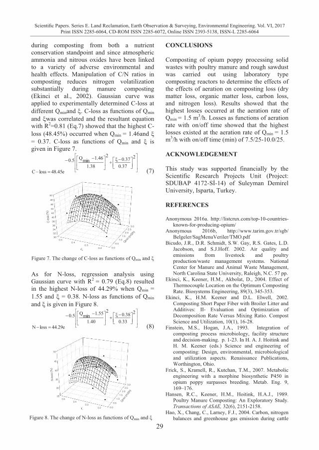
29
Scientific Papers. Series E. Land Reclamation, Earth Observation & Surveying, Environmental Engineering. Vol. VI, 2017Print ISSN 2285-6064, CD-ROM ISSN 2285-6072, Online ISSN 2393-5138, ISSN-L 2285-6064
during composting from both a nutrient conservation standpoint and since atmospheric ammonia and nitrous oxides have been linked to a variety of adverse environmental and health effects. Manipulation of C/N ratios in composting reduces nitrogen volatilization substantially during manure composting (Ekinci et al., 2002). Gaussian curve was applied to experimentally determined C-loss at different Qminand �. C-loss as functions of Qmin and �was correlated and the resultant equation with R2=0.81 (Eq.7) showed that the highest C-loss (48.45%) occurred when Qmin = 1.46and � = 0.37. C-loss as functions of Qmin and � is given in Figure 7.
���
�
�
���
�
�
���
��� ����
�
���
� ��
��
2
37.037.0
2
38.146.1minQ5.0
e45.48lossC (7)
30323436
38
40
42
44
46
48
50
0.0
0.51.0
1.52.0
2.53.0
0.20.3
0.40.5
C-los
s (%
)
Qmin (m3/h
)
Figure 7. The change of C-loss as functions of Qmin and �
As for N-loss, regression analysis using Gaussian curve with R2 = 0.79 (Eq.8) resulted in the highest N-loss of 44.29% when Qmin = 1.55 and � = 0.38. N-loss as functions of Qmin and � is given in Figure 8.
���
�
�
���
�
�
���
��� ����
�
���
� ��
��
2
33.038.0
2
40.155.1minQ5.0
e29.44lossN (8)
25
30
35
40
45
50
0.0
0.51.0
1.52.0
2.53.0
0.20.3
0.40.5
N-lo
ss (%
)
Qmin (m
3/h)
Figure 8. The change of N-loss as functions of Qmin and �
CONCLUSIONS Composting of opium poppy processing solid wastes with poultry manure and rough sawdust was carried out using laboratory type composting reactors to determine the effects of the effects of aeration on composting loss (dry matter loss, organic matter loss, carbon loss, and nitrogen loss). Results showed that the highest losses occurred at the aeration rate of Qmin = 1.5 m3/h. Losses as functions of aeration rate with on/off time showed that the highest losses existed at the aeration rate of Qmin = 1.5 m3/h with on/off time (min) of 7.5/25-10.0/25. ACKNOWLEDGEMENT This study was supported financially by the Scientific Research Projects Unit (Project: SDUBAP 4172-Sİ-14) of Suleyman Demirel University, Isparta, Turkey. REFERENCES Anonymous 2016a. http://listcrux.com/top-10-countries-
known-for-producing-opium/ Anonymous 2016b, http://www.tarim.gov.tr/sgb/
Belgeler/SagMenuVeriler/TMO.pdf Bicudo, J.R., D.R. Schmidt, S.W. Gay, R.S. Gates, L.D.
Jacobson, and S.J.Hoff. 2002. Air quality and emissions from livestock and poultry production/waste management systems. National Center for Manure and Animal Waste Management, North Carolina State University, Raleigh, N.C. 57 pp.
Ekinci, K., Keener, H.M., Akbolat, D., 2004. Effect of Thermocouple Location on the Optimum Composting Rate. Biosystems Engineering, 89(3), 345-353.
Ekinci, K., H.M. Keener and D.L. Elwell, 2002. Composting Short Paper Fiber with Broiler Litter and Additives: II- Evaluation and Optimization of Decomposition Rate Versus Mixing Ratio. Compost Science and Utilization, 10(1), 16-28.
Finstein, M.S., Hogan, J.A., 1993. Integration of composting process microbiology, facility structure and decision-making. p. 1-23. In H. A. J. Hoitink and H. M. Keener (eds.) Science and engineering of composting: Design, environmental, microbiological and utilization aspects. Renaissance Publications, Worthington, Ohio.
Frick, S., Kramell, R., Kutchan, T.M., 2007. Metabolic engineering with a morphine biosynthetic P450 in opium poppy surpasses breeding. Metab. Eng. 9, 169–176.
Hansen, R.C., Keener, H.M., Hoitink, H.A.J., 1989. Poultry Manure Composting: An Exploratory Study. Transactions of ASAE, 32(6), 2151-2158.
Hao, X., Chang, C., Larney, F.J., 2004. Carbon, nitrogen balances and greenhouse gas emission during cattle
30
Scientific Papers. Series E. Land Reclamation, Earth Observation & Surveying, Environmental Engineering. Vol. VI, 2017Print ISSN 2285-6064, CD-ROM ISSN 2285-6072, Online ISSN 2393-5138, ISSN-L 2285-6064
feedlot manure composting. J. Environ. Qual. 33, 37–44.
İpek, G., Arslan, N., 2012. Gıda Maddesi Olarak Haşhaş (Papaver somniferum L.) Tohumunun Değerlendirilmesi. Türk Bilimsel Derlemeler Dergisi 5 (2): 99-101, Kişiselgörüşme, 2015. Afyon Alkaloidleri Fabrikasıpersoneli
Kapoor, L. (1995). Opium poppy: Botany, chemistry and Pharmacology. CRC Press. ISBN: 1560249234.
Keener, H.M., Ekinci, K., Elwell, D.L., Michel, F.C., 2000. Mathematics of composting- facility design and process control. pp. 164-197. In: P.R. Warman and B.R. Taylor (eds.) Proceedings international composting symosium (ICS'99) - Vol. 1. CBA Press Inc., Nova Scotia, Canada.
Larney, F.J., Buckley, K.E., Hao, X., McCaughey, W.P., 2006. Fresh, stockpiled, and composted beef cattle feedlot manure: Nutrient levels and mass balance estimates in Alberta and Manitoba. J. Environ. Qual. 35, 1844–1854.
Mahdavi-Damghani, A., Kamkar, B., Al-Ahmadi, M.J., Testi, L., Muñoz-Ledesmaf, F.J., Villalobos, F.J., 2010. Water stress effects on growth, development and yield of opium poppy (Papaver somniferum L.). Agriculture Water Management, 97, 1582–1590.
Rynk, R. 1992. On-Farm Composting Handbook, Northeast Regional Agricultural Engineering Service, NRAES-54, Ithaca, New York.
TMO, 2011. Official report of opium poppy production. General Directorate of Soil Products Office (TMO), Ankara 2012.
Wijekoon, C.P., Facchini, P.J., 2012. Systematic knockdown of morphine pathway enzymes in opium poppy using virus-induced gene silencing. Plant Journal, 69, 1052–1063.
USCC, 2002. The US Composting Council Research and Education Foundation, and the United States Department of Agriculture. Test methods for the examination of composting and compost (TMECC). Edaphos International, Houston, TX.
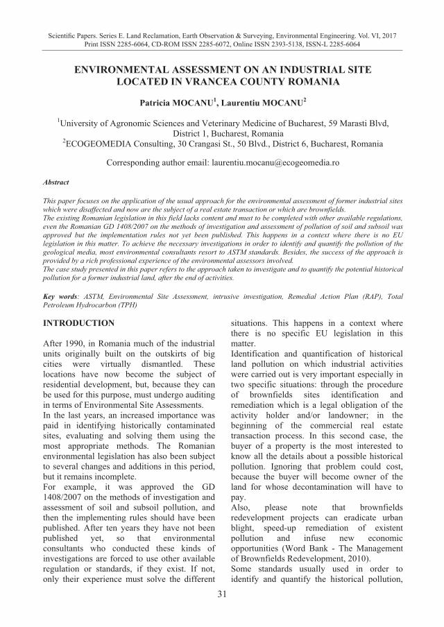
31
Scientific Papers. Series E. Land Reclamation, Earth Observation & Surveying, Environmental Engineering. Vol. VI, 2017Print ISSN 2285-6064, CD-ROM ISSN 2285-6072, Online ISSN 2393-5138, ISSN-L 2285-6064
feedlot manure composting. J. Environ. Qual. 33, 37–44.
İpek, G., Arslan, N., 2012. Gıda Maddesi Olarak Haşhaş (Papaver somniferum L.) Tohumunun Değerlendirilmesi. Türk Bilimsel Derlemeler Dergisi 5 (2): 99-101, Kişiselgörüşme, 2015. Afyon Alkaloidleri Fabrikasıpersoneli
Kapoor, L. (1995). Opium poppy: Botany, chemistry and Pharmacology. CRC Press. ISBN: 1560249234.
Keener, H.M., Ekinci, K., Elwell, D.L., Michel, F.C., 2000. Mathematics of composting- facility design and process control. pp. 164-197. In: P.R. Warman and B.R. Taylor (eds.) Proceedings international composting symosium (ICS'99) - Vol. 1. CBA Press Inc., Nova Scotia, Canada.
Larney, F.J., Buckley, K.E., Hao, X., McCaughey, W.P., 2006. Fresh, stockpiled, and composted beef cattle feedlot manure: Nutrient levels and mass balance estimates in Alberta and Manitoba. J. Environ. Qual. 35, 1844–1854.
Mahdavi-Damghani, A., Kamkar, B., Al-Ahmadi, M.J., Testi, L., Muñoz-Ledesmaf, F.J., Villalobos, F.J., 2010. Water stress effects on growth, development and yield of opium poppy (Papaver somniferum L.). Agriculture Water Management, 97, 1582–1590.
Rynk, R. 1992. On-Farm Composting Handbook, Northeast Regional Agricultural Engineering Service, NRAES-54, Ithaca, New York.
TMO, 2011. Official report of opium poppy production. General Directorate of Soil Products Office (TMO), Ankara 2012.
Wijekoon, C.P., Facchini, P.J., 2012. Systematic knockdown of morphine pathway enzymes in opium poppy using virus-induced gene silencing. Plant Journal, 69, 1052–1063.
USCC, 2002. The US Composting Council Research and Education Foundation, and the United States Department of Agriculture. Test methods for the examination of composting and compost (TMECC). Edaphos International, Houston, TX.
ENVIRONMENTAL ASSESSMENT ON AN INDUSTRIAL SITE
LOCATED IN VRANCEA COUNTY ROMANIA
Patricia MOCANU1, Laurentiu MOCANU2
1University of Agronomic Sciences and Veterinary Medicine of Bucharest, 59 Marasti Blvd, District 1, Bucharest, Romania
2ECOGEOMEDIA Consulting, 30 Crangasi St., 50 Blvd., District 6, Bucharest, Romania
Corresponding author email: [email protected] Abstract This paper focuses on the application of the usual approach for the environmental assessment of former industrial sites which were disaffected and now are the subject of a real estate transaction or which are brownfields. The existing Romanian legislation in this field lacks content and must to be completed with other available regulations, even the Romanian GD 1408/2007 on the methods of investigation and assessment of pollution of soil and subsoil was approved but the implementation rules not yet been published. This happens in a context where there is no EU legislation in this matter. To achieve the necessary investigations in order to identify and quantify the pollution of the geological media, most environmental consultants resort to ASTM standards. Besides, the success of the approach is provided by a rich professional experience of the environmental assessors involved. The case study presented in this paper refers to the approach taken to investigate and to quantify the potential historical pollution for a former industrial land, after the end of activities. Key words: ASTM, Environmental Site Assessment, intrusive investigation, Remedial Action Plan (RAP), Total Petroleum Hydrocarbon (TPH) INTRODUCTION After 1990, in Romania much of the industrial units originally built on the outskirts of big cities were virtually dismantled. These locations have now become the subject of residential development, but, because they can be used for this purpose, must undergo auditing in terms of Environmental Site Assessments. In the last years, an increased importance was paid in identifying historically contaminated sites, evaluating and solving them using the most appropriate methods. The Romanian environmental legislation has also been subject to several changes and additions in this period, but it remains incomplete. For example, it was approved the GD 1408/2007 on the methods of investigation and assessment of soil and subsoil pollution, and then the implementing rules should have been published. After ten years they have not been published yet, so that environmental consultants who conducted these kinds of investigations are forced to use other available regulation or standards, if they exist. If not, only their experience must solve the different
situations. This happens in a context where there is no specific EU legislation in this matter. Identification and quantification of historical land pollution on which industrial activities were carried out is very important especially in two specific situations: through the procedure of brownfields sites identification and remediation which is a legal obligation of the activity holder and/or landowner; in the beginning of the commercial real estate transaction process. In this second case, the buyer of a property is the most interested to know all the details about a possible historical pollution. Ignoring that problem could cost, because the buyer will become owner of the land for whose decontamination will have to pay. Also, please note that brownfields redevelopment projects can eradicate urban blight, speed-up remediation of existent pollution and infuse new economic opportunities (Word Bank - The Management of Brownfields Redevelopment, 2010). Some standards usually used in order to identify and quantify the historical pollution,
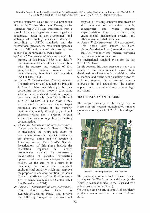
32
Scientific Papers. Series E. Land Reclamation, Earth Observation & Surveying, Environmental Engineering. Vol. VI, 2017Print ISSN 2285-6064, CD-ROM ISSN 2285-6072, Online ISSN 2393-5138, ISSN-L 2285-6064
are the standards issued by ASTM (American Society for Testing Materials). Throughout its existence, the ASTM was transformed from a simple American organization into a globally recognized leader in the development and delivery of voluntary consensus standards. According to ASTM standards and the international practice, the most usual approach for the full environmental site assessments requires going through following steps: a) Phase I Environmental Site Assessment. The
purpose of this Phase I ESA is to identify the environmental conditions in connection with the property and consists of four components: records review, site reconnaissance, interviews and reporting (ASTM E1527-13);
b) Phase II Environmental Site Assessment. The main objective of conducting a Phase II ESA is to obtain scientifically valid data concerning the actual property conditions, whether or not such data relate to property conditions previously identified in Phase I ESA (ASTM E1903-11). The Phase II ESA is conducted to determine whether target pollutants are present in the property environment, mainly through physical and chemical testing, and if present, to gain sufficient information regarding the existing contamination.
c) Phase III Environmental Site Assessment. The primary objective of a Phase III ESA is to investigate the nature and extent of adverse environmental impact identified by the previous phase and to develop a Remedial Action Plan (RAP). Specific investigations of this phase include the calculation impacted soil and/or groundwater volume, risk assessment, identification of possible remediation options, and sometimes site-specific pilot studies. At the end of this stage it is mandatory to notify the competent environmental authority which must approve the proposed remediation solution (Canadian Council of Ministers of the Environment - Environmental Guideline for Contaminated Site Remediation, 2003).
d) Phase IV Environmental Site Assessment. This phase (also known as Remediation/clean-up Phase) may involve the following components: removal and
disposal of existing contaminated areas; on site treatment of contaminated soils, groundwater and waste streams; implementation of waste reduction plans, environmental management systems, and other source remedial measures.
e) Phase V Environmental Site Assessment. This phase (also known as Com-pletion/Validation Phase) must demonstrate that RAP was fully implemented, providing evidence of actions undertaken.
No international standard exists for the last three ESA phases. In this context, this paper presents a study case related to the environmental investigations developed on a Romanian brownfield, in order to identify and quantify the existing historical pollution, required by a potential investor interested in land acquisition. The authors applied both national and international legal provisions. MATERIALS AND METHODS The subject property of the study case is located in the Focsani municipality, Vrancea County and occupies 19,382 m2 of land (Figure 1).
Figure 1. Site map location (INIS Viewer)
The property is bordered by the Buzau – Bacau railway (to the West), an industrial area (to the North), a residential area (to the East) and by a public property (to the South). On the subject property a deposit of petroleum products was in operation between 1952 and 2012.
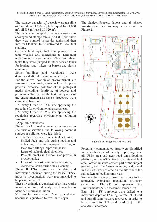
33
Scientific Papers. Series E. Land Reclamation, Earth Observation & Surveying, Environmental Engineering. Vol. VI, 2017Print ISSN 2285-6064, CD-ROM ISSN 2285-6072, Online ISSN 2393-5138, ISSN-L 2285-6064
The storage capacity of deposit was: gasoline 640 m3; diesel 1,966 m3; light liquid fuel 1,030 m3; oil 588 m3; used oil 120 m3. The fuels were pumped from tank wagons into aboveground storage tanks (ASTs). From there they were pumped in service tanks and then into road tankers, to be delivered to local fuel stations. Oils and light liquid fuel were pumped from tank wagons and discharged to horizontal underground storage tanks (USTs). From these tanks they were pumped to other service tanks for loading road tankers, or barrels and plastic containers. Some buildings and warehouses were demolished after the cessation of activity. For the above location an environmental site assessment was made, aimed at identifying the potential historical pollution of the geological media (including identifying of sources and pollutants). To this end, the first three phases of the environmental assessment procedure were completed based on: - Ministry Order no. 184/1997 approving the procedure for environmental assessments; - Ministry Order no. 756/1997 approving the regulation regarding environmental pollution assessment; - Applicable standards. Phase I ESA. Based on records review and on site visit observation, the following potential sources of pollution were identified: - Traffic emissions from the tanker trunks; - Spilled fuels and oils during loading and
unloading, due to improper handling or leaks from fittings, pipes and hoses;
- Leaks of technological pipelines; - Possible cracks in the walls of petroleum
product tanks; - Leaks of the wastewater sewage system; - Accidental spills during tank cleaning.
Phase II ESA. Based on the data and information obtained during the Phase I ESA, intrusive investigations were recommended to be performed on site. These investigations consisted of drilling works in order to take and analyze soil samples to identify historical pollution. No samples were taken from groundwater because it is quartered to over 20 m depth.
The Subject Property layout and all phases investigation locations map are enclosed in Figure 2.
Figure 2. Investigation locations map
Potentially contaminated areas were identified in the northern part of the subject property, near oil USTs area and near road tanks loading platform, in the ASTs formerly contained fuel area, located in south-eastern part of the subject property, near the former pumping station and in the north-western area on the site where the rail tankers unloading ramp was. Soil sampling was performed according to the applicable Romanian regulations (Ministry Order no. 184/1997 on approving the Environmental Site Assessment Procedure). Eight (F1 – F8) boreholes were drilled to a maximum depth of 12 m bgl; a total of 31 soil and subsoil samples were recovered in order to be analyzed for TPH and Lead (Pb) in the analytical laboratory.
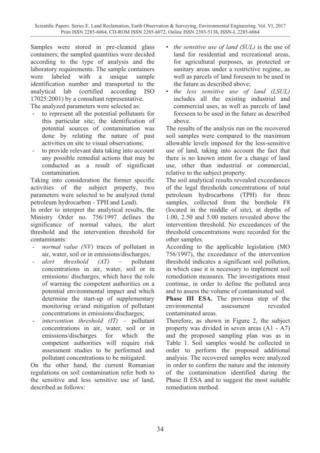
34
Scientific Papers. Series E. Land Reclamation, Earth Observation & Surveying, Environmental Engineering. Vol. VI, 2017Print ISSN 2285-6064, CD-ROM ISSN 2285-6072, Online ISSN 2393-5138, ISSN-L 2285-6064
Samples were stored in pre-cleaned glass containers; the sampled quantities were decided according to the type of analysis and the laboratory requirements. The sample containers were labeled with a unique sample identification number and transported to the analytical lab (certified according ISO 17025:2001) by a consultant representative. The analyzed parameters were selected as: - to represent all the potential pollutants for
this particular site; the identification of potential sources of contamination was done by relating the nature of past activities on site to visual observations;
- to provide relevant data taking into account any possible remedial actions that may be conducted as a result of significant contamination.
Taking into consideration the former specific activities of the subject property, two parameters were selected to be analyzed (total petroleum hydrocarbon - TPH and Lead). In order to interpret the analytical results, the Ministry Order no. 756/1997 defines the significance of normal values, the alert threshold and the intervention threshold for contaminants: - normal value (NV) traces of pollutant in
air, water, soil or in emissions/discharges; - alert threshold (AT) – pollutant
concentrations in air, water, soil or in emissions/ discharges, which have the role of warning the competent authorities on a potential environmental impact and which determine the start-up of supplementary monitoring or/and mitigation of pollutant concentrations in emissions/discharges;
- intervention threshold (IT) – pollutant concentrations in air, water, soil or in emissions/discharges for which the competent authorities will require risk assessment studies to be performed and pollutant concentrations to be mitigated.
On the other hand, the current Romanian regulations on soil contamination refer both to the sensitive and less sensitive use of land, described as follows:
• the sensitive use of land (SUL) is the use of land for residential and recreational areas, for agricultural purposes, as protected or sanitary areas under a restrictive regime, as well as parcels of land foreseen to be used in the future as described above;
• the less sensitive use of land (LSUL) includes all the existing industrial and commercial uses, as well as parcels of land foreseen to be used in the future as described above.
The results of the analysis run on the recovered soil samples were compared to the maximum allowable levels imposed for the less-sensitive use of land, taking into account the fact that there is no known intent for a change of land use, other than industrial or commercial, relative to the subject property. The soil analytical results revealed exceedances of the legal thresholds concentrations of total petroleum hydrocarbons (TPH) for three samples, collected from the borehole F8 (located in the middle of site), at depths of 1.00, 2.50 and 5.00 meters revealed above the intervention threshold. No exceedances of the threshold concentrations were recorded for the other samples. According to the applicable legislation (MO 756/1997), the exceedance of the intervention threshold indicates a significant soil pollution, in which case it is necessary to implement soil remediation measures. The investigations must continue, in order to define the polluted area and to assess the volume of contaminated soil. Phase III ESA. The previous step of the environmental assessment revealed contaminated areas. Therefore, as shown in Figure 2, the subject property was divided in seven areas (A1 - A7) and the proposed sampling plan was as in Table 1. Soil samples would be collected in order to perform the proposed additional analysis. The recovered samples were analyzed in order to confirm the nature and the intensity of the contamination identified during the Phase II ESA and to suggest the most suitable remediation method.
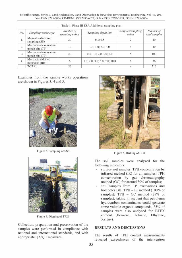
35
Scientific Papers. Series E. Land Reclamation, Earth Observation & Surveying, Environmental Engineering. Vol. VI, 2017Print ISSN 2285-6064, CD-ROM ISSN 2285-6072, Online ISSN 2393-5138, ISSN-L 2285-6064
Samples were stored in pre-cleaned glass containers; the sampled quantities were decided according to the type of analysis and the laboratory requirements. The sample containers were labeled with a unique sample identification number and transported to the analytical lab (certified according ISO 17025:2001) by a consultant representative. The analyzed parameters were selected as: - to represent all the potential pollutants for
this particular site; the identification of potential sources of contamination was done by relating the nature of past activities on site to visual observations;
- to provide relevant data taking into account any possible remedial actions that may be conducted as a result of significant contamination.
Taking into consideration the former specific activities of the subject property, two parameters were selected to be analyzed (total petroleum hydrocarbon - TPH and Lead). In order to interpret the analytical results, the Ministry Order no. 756/1997 defines the significance of normal values, the alert threshold and the intervention threshold for contaminants: - normal value (NV) traces of pollutant in
air, water, soil or in emissions/discharges; - alert threshold (AT) – pollutant
concentrations in air, water, soil or in emissions/ discharges, which have the role of warning the competent authorities on a potential environmental impact and which determine the start-up of supplementary monitoring or/and mitigation of pollutant concentrations in emissions/discharges;
- intervention threshold (IT) – pollutant concentrations in air, water, soil or in emissions/discharges for which the competent authorities will require risk assessment studies to be performed and pollutant concentrations to be mitigated.
On the other hand, the current Romanian regulations on soil contamination refer both to the sensitive and less sensitive use of land, described as follows:
• the sensitive use of land (SUL) is the use of land for residential and recreational areas, for agricultural purposes, as protected or sanitary areas under a restrictive regime, as well as parcels of land foreseen to be used in the future as described above;
• the less sensitive use of land (LSUL) includes all the existing industrial and commercial uses, as well as parcels of land foreseen to be used in the future as described above.
The results of the analysis run on the recovered soil samples were compared to the maximum allowable levels imposed for the less-sensitive use of land, taking into account the fact that there is no known intent for a change of land use, other than industrial or commercial, relative to the subject property. The soil analytical results revealed exceedances of the legal thresholds concentrations of total petroleum hydrocarbons (TPH) for three samples, collected from the borehole F8 (located in the middle of site), at depths of 1.00, 2.50 and 5.00 meters revealed above the intervention threshold. No exceedances of the threshold concentrations were recorded for the other samples. According to the applicable legislation (MO 756/1997), the exceedance of the intervention threshold indicates a significant soil pollution, in which case it is necessary to implement soil remediation measures. The investigations must continue, in order to define the polluted area and to assess the volume of contaminated soil. Phase III ESA. The previous step of the environmental assessment revealed contaminated areas. Therefore, as shown in Figure 2, the subject property was divided in seven areas (A1 - A7) and the proposed sampling plan was as in Table 1. Soil samples would be collected in order to perform the proposed additional analysis. The recovered samples were analyzed in order to confirm the nature and the intensity of the contamination identified during the Phase II ESA and to suggest the most suitable remediation method.
Table 1. Phase III ESA Additional sampling plan
No. Sampling works type Number of sampling points Sampling depth (m) Samples/sampling
points Number of
total samples
1. Manual surface soil sampling (SS) 20 0.3; 0.5 2 40
2. Mechanical excavation trench pits (TP) 10 0.3; 1.0; 2.0; 3.0 4 40
3 Mechanical excavation trench pits (TP) 20 0.3; 1.0; 2.0; 3.0; 5.0 5 100
4. Mechanical drilled boreholes (BH) 6 1.0; 2.0; 3.0; 5.0; 7.0; 10.0 6 36
TOTAL 56 - - 216 Examples from the sample works operations are shown in Figures 3, 4 and 5.
Figure 3. Sampling of SS3
Figure 4. Digging of TP26
Collection, preparation and preservation of the samples were performed in compliance with national and international standards, and with appropriate QA/QC measures.
Figure 5. Drilling of BH4
The soil samples were analyzed for the following indicators: - surface soil samples: TPH concentration by
infrared method (IR) for all samples; TPH concentration by gas chromatography method (GC) for around 30% of samples;
- soil samples from TP excavations and boreholes BH: TPH – IR method (100% of samples); TPH – GC method (28% of samples); taking in account that petroleum hydrocarbon contaminants could generate some volatile organic compounds, 35% of samples were also analysed for BTEX content (Benzene, Toluene, Ethylene, Xylene).
RESULTS AND DISCUSSIONS The results of TPH content measurements revealed exceedances of the intervention
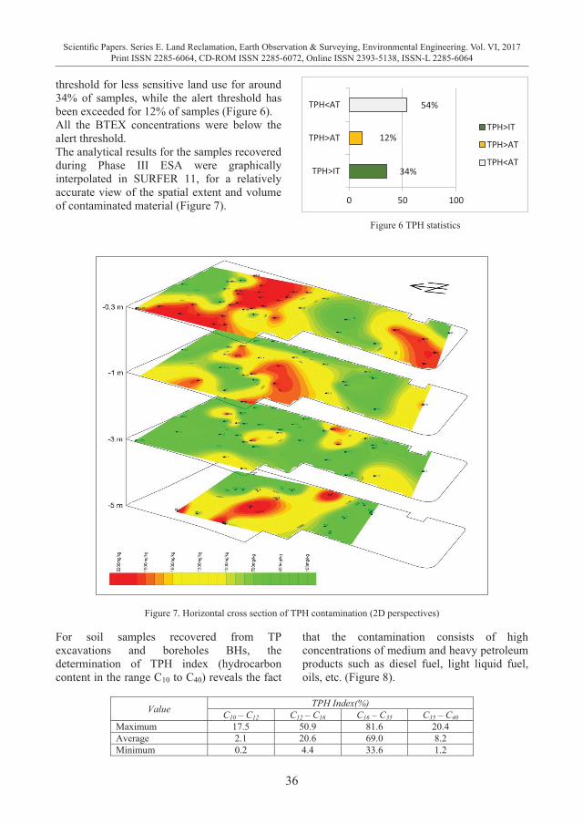
36
Scientific Papers. Series E. Land Reclamation, Earth Observation & Surveying, Environmental Engineering. Vol. VI, 2017Print ISSN 2285-6064, CD-ROM ISSN 2285-6072, Online ISSN 2393-5138, ISSN-L 2285-6064
threshold for less sensitive land use for around 34% of samples, while the alert threshold has been exceeded for 12% of samples (Figure 6). All the BTEX concentrations were below the alert threshold. The analytical results for the samples recovered during Phase III ESA were graphically interpolated in SURFER 11, for a relatively accurate view of the spatial extent and volume of contaminated material (Figure 7).
Figure 6 TPH statistics
Figure 7. Horizontal cross section of TPH contamination (2D perspectives) For soil samples recovered from TP excavations and boreholes BHs, the determination of TPH index (hydrocarbon content in the range C10 to C40) reveals the fact
that the contamination consists of high concentrations of medium and heavy petroleum products such as diesel fuel, light liquid fuel, oils, etc. (Figure 8).
34%
12%
54%
0 50 100
TPH>IT
TPH>AT
TPH<AT
TPH>IT
TPH>AT
TPH<AT
Value TPH Index(%) C10 – C12 C12 – C16 C16 – C35 C35 – C40
Maximum 17.5 50.9 81.6 20.4 Average 2.1 20.6 69.0 8.2 Minimum 0.2 4.4 33.6 1.2
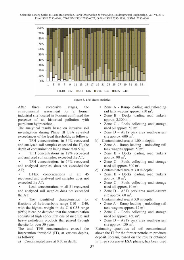
37
Scientific Papers. Series E. Land Reclamation, Earth Observation & Surveying, Environmental Engineering. Vol. VI, 2017Print ISSN 2285-6064, CD-ROM ISSN 2285-6072, Online ISSN 2393-5138, ISSN-L 2285-6064
threshold for less sensitive land use for around 34% of samples, while the alert threshold has been exceeded for 12% of samples (Figure 6). All the BTEX concentrations were below the alert threshold. The analytical results for the samples recovered during Phase III ESA were graphically interpolated in SURFER 11, for a relatively accurate view of the spatial extent and volume of contaminated material (Figure 7).
Figure 6 TPH statistics
Figure 7. Horizontal cross section of TPH contamination (2D perspectives) For soil samples recovered from TP excavations and boreholes BHs, the determination of TPH index (hydrocarbon content in the range C10 to C40) reveals the fact
that the contamination consists of high concentrations of medium and heavy petroleum products such as diesel fuel, light liquid fuel, oils, etc. (Figure 8).
34%
12%
54%
0 50 100
TPH>IT
TPH>AT
TPH<AT
TPH>IT
TPH>AT
TPH<AT
Value TPH Index(%) C10 – C12 C12 – C16 C16 – C35 C35 – C40
Maximum 17.5 50.9 81.6 20.4 Average 2.1 20.6 69.0 8.2 Minimum 0.2 4.4 33.6 1.2
Figure 8. TPH Index statistics
After three successive stages, the environmental assessment for a former industrial site located in Focsani confirmed the presence of an historical pollution with petroleum hydrocarbon. The analytical results based on intrusive soil investigation during Phase III ESA revealed exceedances of the legal thresholds, as follows: • TPH concentrations in 34% recovered
and analysed soil samples exceeded the IT, the depth of contamination being more than 5 m; • TPH concentrations in 12% recovered
and analysed soil samples, exceeded the AT; • TPH concentrations in 54% recovered
and analysed samples, does not exceeded the AT; • BTEX concentrations in all 45
recovered and analysed soil samples does not exceeded the AT; • Lead concentrations in all 31 recovered
and analysed soil samples does not exceeded the AT; • The identified characteristics for
fractions of hydrocarbons range C10 – C40, with the highest weight in the C16-C35 range (69%) it can be deduced that the contamination consists of high concentrations of medium and heavy petroleum products that passed through the site for over 50 years. The total TPH concentrations exceed the intervention threshold (IT), at various depths, as follows: a) Contaminated area at 0.30 m depth:
• Zone A - Ramp loading and unloading rail tank wagons approx. 950 m2;
• Zone B - Decks loading road tankers approx. 2.300 m2;
• Zone C - Pools collecting and storage used oil approx. 50 m2;
• Zone D – ASTs park area south-eastern site approx. 600 m2.
b) Contaminated area at 1.00 m depth: • Zone A - Ramp loading - unloading rail
tank wagons approx. 50m2; • Zone B - Decks loading road tankers
approx. 90 m2; • Zone C - Pools collecting and storage
used oil approx. 500 m2. c) Contaminated area at 3.0 m depth:
• Zone B - Decks loading road tankers approx. 10 m2;
• Zone C - Pools collecting and storage used oil approx. 10 m2;
• Zone D – ASTs park area south-eastern site approx. 60 m2.
d) Contaminated area at 5.0 m depth: • Zone A - Ramp loading - unloading rail
tank wagons approx. 12 m2; • Zone C - Pools collecting and storage
used oil approx. 450 m2; • Zone D – ASTs park area south-eastern
site approx. 130 m2. Estimating quantities of soil contaminated above the IT for the former petroleum products deposit Focsani, based on the results obtained in three successive ESA phases, has been used
0%
10%
20%
30%
40%
50%
60%
70%
80%
90%
100%
1 3 5 7 9 11 13 15 17 19 21 23 25 27 29 31 33 35
C10 – C12 C12 – C16 C16 – C35 C35 – C40
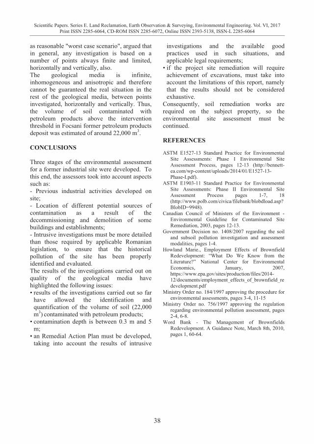
38
Scientific Papers. Series E. Land Reclamation, Earth Observation & Surveying, Environmental Engineering. Vol. VI, 2017Print ISSN 2285-6064, CD-ROM ISSN 2285-6072, Online ISSN 2393-5138, ISSN-L 2285-6064
as reasonable "worst case scenario", argued that in general, any investigation is based on a number of points always finite and limited, horizontally and vertically, also. The geological media is infinite, inhomogeneous and anisotropic and therefore cannot be guaranteed the real situation in the rest of the geological media, between points investigated, horizontally and vertically. Thus, the volume of soil contaminated with petroleum products above the intervention threshold in Focsani former petroleum products deposit was estimated of around 22,000 m3. CONCLUSIONS Three stages of the environmental assessment for a former industrial site were developed. To this end, the assessors took into account aspects such as: - Previous industrial activities developed on site; - Location of different potential sources of contamination as a result of the decommissioning and demolition of some buildings and establishments; - Intrusive investigations must be more detailed than those required by applicable Romanian legislation, to ensure that the historical pollution of the site has been properly identified and evaluated. The results of the investigations carried out on quality of the geological media have highlighted the following issues: • results of the investigations carried out so far
have allowed the identification and quantification of the volume of soil (22,000 m3) contaminated with petroleum products;
• contamination depth is between 0.3 m and 5 m;
• an Remedial Action Plan must be developed, taking into account the results of intrusive
investigations and the available good practices used in such situations, and applicable legal requirements;
• if the project site remediation will require achievement of excavations, must take into account the limitations of this report, namely that the results should not be considered exhaustive.
Consequently, soil remediation works are required on the subject property, so the environmental site assessment must be continued. REFERENCES ASTM E1527-13 Standard Practice for Environmental
Site Assessments: Phase I Environmental Site Assessment Process, pages 12-13 (http://bennett-ea.com/wp-content/uploads/2014/01/E1527-13-Phase-I.pdf).
ASTM E1903-11 Standard Practice for Environmental Site Assessments: Phase II Environmental Site Assessment Process pages 1-7, 18 (http://www.polb.com/civica/filebank/blobdload.asp?BlobID=9948).
Canadian Council of Ministers of the Environment - Environmental Guideline for Contaminated Site Remediation, 2003, pages 12-13.
Government Decision no. 1408/2007 regarding the soil and subsoil pollution investigation and assessment modalities, pages 1-4.
Howland Marie., Employment Effects of Brownfield Redevelopment: “What Do We Know from the Literature?” National Center for Environmental Economics, January, 2007, https://www.epa.gov/sites/production/files/2014-12/documents/employment_effects_of_brownfield_redevelopment.pdf
Ministry Order no. 184/1997 approving the procedure for environmental assessments, pages 3-4, 11-15
Ministry Order no. 756/1997 approving the regulation regarding environmental pollution assessment, pages 2-4, 6-8.
Word Bank - The Management of Brownfields Redevelopment. A Guidance Note, March 8th, 2010, pages 1, 60-64.
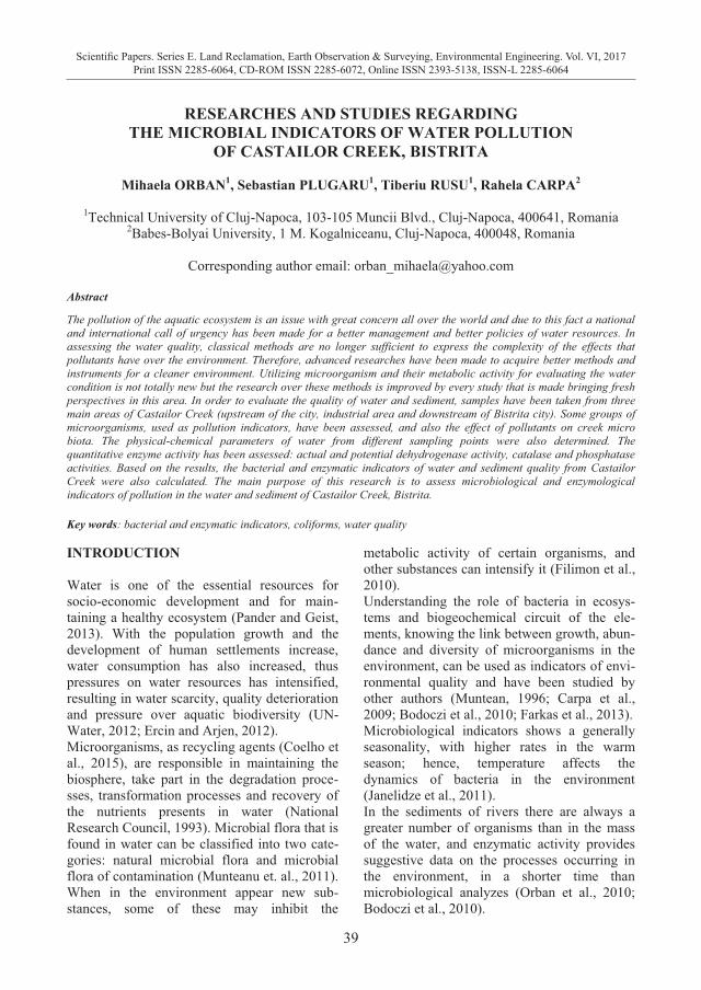
39
Scientific Papers. Series E. Land Reclamation, Earth Observation & Surveying, Environmental Engineering. Vol. VI, 2017Print ISSN 2285-6064, CD-ROM ISSN 2285-6072, Online ISSN 2393-5138, ISSN-L 2285-6064
as reasonable "worst case scenario", argued that in general, any investigation is based on a number of points always finite and limited, horizontally and vertically, also. The geological media is infinite, inhomogeneous and anisotropic and therefore cannot be guaranteed the real situation in the rest of the geological media, between points investigated, horizontally and vertically. Thus, the volume of soil contaminated with petroleum products above the intervention threshold in Focsani former petroleum products deposit was estimated of around 22,000 m3. CONCLUSIONS Three stages of the environmental assessment for a former industrial site were developed. To this end, the assessors took into account aspects such as: - Previous industrial activities developed on site; - Location of different potential sources of contamination as a result of the decommissioning and demolition of some buildings and establishments; - Intrusive investigations must be more detailed than those required by applicable Romanian legislation, to ensure that the historical pollution of the site has been properly identified and evaluated. The results of the investigations carried out on quality of the geological media have highlighted the following issues: • results of the investigations carried out so far
have allowed the identification and quantification of the volume of soil (22,000 m3) contaminated with petroleum products;
• contamination depth is between 0.3 m and 5 m;
• an Remedial Action Plan must be developed, taking into account the results of intrusive
investigations and the available good practices used in such situations, and applicable legal requirements;
• if the project site remediation will require achievement of excavations, must take into account the limitations of this report, namely that the results should not be considered exhaustive.
Consequently, soil remediation works are required on the subject property, so the environmental site assessment must be continued. REFERENCES ASTM E1527-13 Standard Practice for Environmental
Site Assessments: Phase I Environmental Site Assessment Process, pages 12-13 (http://bennett-ea.com/wp-content/uploads/2014/01/E1527-13-Phase-I.pdf).
ASTM E1903-11 Standard Practice for Environmental Site Assessments: Phase II Environmental Site Assessment Process pages 1-7, 18 (http://www.polb.com/civica/filebank/blobdload.asp?BlobID=9948).
Canadian Council of Ministers of the Environment - Environmental Guideline for Contaminated Site Remediation, 2003, pages 12-13.
Government Decision no. 1408/2007 regarding the soil and subsoil pollution investigation and assessment modalities, pages 1-4.
Howland Marie., Employment Effects of Brownfield Redevelopment: “What Do We Know from the Literature?” National Center for Environmental Economics, January, 2007, https://www.epa.gov/sites/production/files/2014-12/documents/employment_effects_of_brownfield_redevelopment.pdf
Ministry Order no. 184/1997 approving the procedure for environmental assessments, pages 3-4, 11-15
Ministry Order no. 756/1997 approving the regulation regarding environmental pollution assessment, pages 2-4, 6-8.
Word Bank - The Management of Brownfields Redevelopment. A Guidance Note, March 8th, 2010, pages 1, 60-64.
RESEARCHES AND STUDIES REGARDING THE MICROBIAL INDICATORS OF WATER POLLUTION
OF CASTAILOR CREEK, BISTRITA
Mihaela ORBAN1, Sebastian PLUGARU1, Tiberiu RUSU1, Rahela CARPA2
1Technical University of Cluj-Napoca, 103-105 Muncii Blvd., Cluj-Napoca, 400641, Romania 2Babes-Bolyai University, 1 M. Kogalniceanu, Cluj-Napoca, 400048, Romania
Corresponding author email: [email protected]
Abstract The pollution of the aquatic ecosystem is an issue with great concern all over the world and due to this fact a national and international call of urgency has been made for a better management and better policies of water resources. In assessing the water quality, classical methods are no longer sufficient to express the complexity of the effects that pollutants have over the environment. Therefore, advanced researches have been made to acquire better methods and instruments for a cleaner environment. Utilizing microorganism and their metabolic activity for evaluating the water condition is not totally new but the research over these methods is improved by every study that is made bringing fresh perspectives in this area. In order to evaluate the quality of water and sediment, samples have been taken from three main areas of Castailor Creek (upstream of the city, industrial area and downstream of Bistrita city). Some groups of microorganisms, used as pollution indicators, have been assessed, and also the effect of pollutants on creek micro biota. The physical-chemical parameters of water from different sampling points were also determined. The quantitative enzyme activity has been assessed: actual and potential dehydrogenase activity, catalase and phosphatase activities. Based on the results, the bacterial and enzymatic indicators of water and sediment quality from Castailor Creek were also calculated. The main purpose of this research is to assess microbiological and enzymological indicators of pollution in the water and sediment of Castailor Creek, Bistrita. Key words: bacterial and enzymatic indicators, coliforms, water quality INTRODUCTION Water is one of the essential resources for socio-economic development and for main-taining a healthy ecosystem (Pander and Geist, 2013). With the population growth and the development of human settlements increase, water consumption has also increased, thus pressures on water resources has intensified, resulting in water scarcity, quality deterioration and pressure over aquatic biodiversity (UN-Water, 2012; Ercin and Arjen, 2012). Microorganisms, as recycling agents (Coelho et al., 2015), are responsible in maintaining the biosphere, take part in the degradation proce-sses, transformation processes and recovery of the nutrients presents in water (National Research Council, 1993). Microbial flora that is found in water can be classified into two cate-gories: natural microbial flora and microbial flora of contamination (Munteanu et. al., 2011). When in the environment appear new sub-stances, some of these may inhibit the
metabolic activity of certain organisms, and other substances can intensify it (Filimon et al., 2010). Understanding the role of bacteria in ecosys-tems and biogeochemical circuit of the ele-ments, knowing the link between growth, abun-dance and diversity of microorganisms in the environment, can be used as indicators of envi-ronmental quality and have been studied by other authors (Muntean, 1996; Carpa et al., 2009; Bodoczi et al., 2010; Farkas et al., 2013). Microbiological indicators shows a generally seasonality, with higher rates in the warm season; hence, temperature affects the dynamics of bacteria in the environment (Janelidze et al., 2011). In the sediments of rivers there are always a greater number of organisms than in the mass of the water, and enzymatic activity provides suggestive data on the processes occurring in the environment, in a shorter time than microbiological analyzes (Orban et al., 2010; Bodoczi et al., 2010).
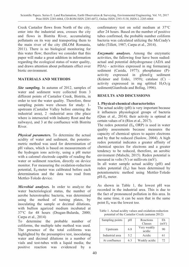
40
Scientific Papers. Series E. Land Reclamation, Earth Observation & Surveying, Environmental Engineering. Vol. VI, 2017Print ISSN 2285-6064, CD-ROM ISSN 2285-6072, Online ISSN 2393-5138, ISSN-L 2285-6064
Creek Castailor flows from North of the city, enter into the industrial area, crosses the city and flows in Bistrita River, accumulating pollutants on its way and transporting them to the main river of the city (BLOM Romania, 2011). There is no biological monitoring for this water flow; therefore we consider that this paper will make a great addition in information regarding the ecological status of water quality, and draws attention about pollutants effect over biotic environment. MATERIALS AND METHODS Site sampling. In autumn of 2012, samples of water and sediment were collected from 3 different points of Castailor Creek, Bistrita, in order to test the water quality. Therefore, three sampling points were chosen for study: 1-upstream (Castailor Valley before entering the industrial area), 2 -industrial area (the place where is intersected with Industry Rout and the railways), and 3 at the confluence with Bistrita River. Physical parameters. To determine the actual acidity of water and sediment, the potentio-metric method was used for determination of pH values, which is based on measurements of the hydrogen ions activity, using a pH meter with a calomel electrode capable of reading the water or sediment reaction, directly on device monitor. For measuring the oxidation-reduction potential, Eh-meter was calibrated before each determination and the data was read from Mettler-Toledo device. Microbial analyses. In order to analyze the water bacteriological status, the number of aerobe heterotrophic bacteria, was determined using the method of turning plates, by inoculating the sample or decimal dilutions, with bullion agarized medium incubated at 37°C for 48 hours (Dragan-Bularda, 2000; Carpa et al., 2014) To determine the probable number of coliforms, the multiple tube method was used. The presence of the total coliforms was highlighted by the presumptive test, inoculating water and decimal dilutions in a number of vials and test-tubes with a liquid media; the positive reaction was evidenced by a
confirmatory test on solid medium at 37°C after 24 hours. Based on the number of positive tubes confirmed, the probable number coliform bacteria was calculated utilizing the McCrady's table (Tillett, 1987; Carpa et al., 2014). Enzymatic analyses. Among the enzymatic activities, the fallowing four have been sudied: actual and potential dehydrogenase (ADA and PDA) - activities expressed in mg formazan/g sediment (Casida, 1977); phosphatase (P)- activity expressed in gfenol/g sediment (Krámer and Erdei, 1959); catalase (C) –activity expresssed in mg splitted H2O2/g sediment(Gianfreda and Bollag, 1996). RESULTS AND DISCUSSIONS 1. Physical-chemical characteristics The actual acidity (pH) is very important because it influences physiological groups of bacteria (Qian et al., 2014); their activity is optimal at certain values of it (Ríos et al., 2017). The redox potential (Eh, ORP) is used in water quality assessments because measures the capacity of chemical spices to aquire electrons and by that be reduced (Suslow, 2004). A high redox potential indicates a greater affinity of chemical species for electrons and a greater tendency to be reduced, therefore, an aerobic enviroment (Malschi, 2015). Redox potential is mesured in volts (V) or millivots (mV). In all water sample actual acidity (pH) and redox potential (Eh) has been determined by potentiometric method using Mettler-Toledo pH-Eh meter. As shown in Table 1, the lowest pH was recorded in the industrial area. This is due to the fact of pronounced pollution in this area. In the same time, it can be seen that in the same point Eh was the lowest too.
Table 1. Actual acidity values and oxidation-reduction potential of the Castailor Creek (autumn 2012)
Sampling points pH Reactions Classes
Eh (mV)
Upstream 6.8 Very weakly acidic 90
Industrial area 5.2 Acidic 61 At confluence 6.3 Weakly acidic 72
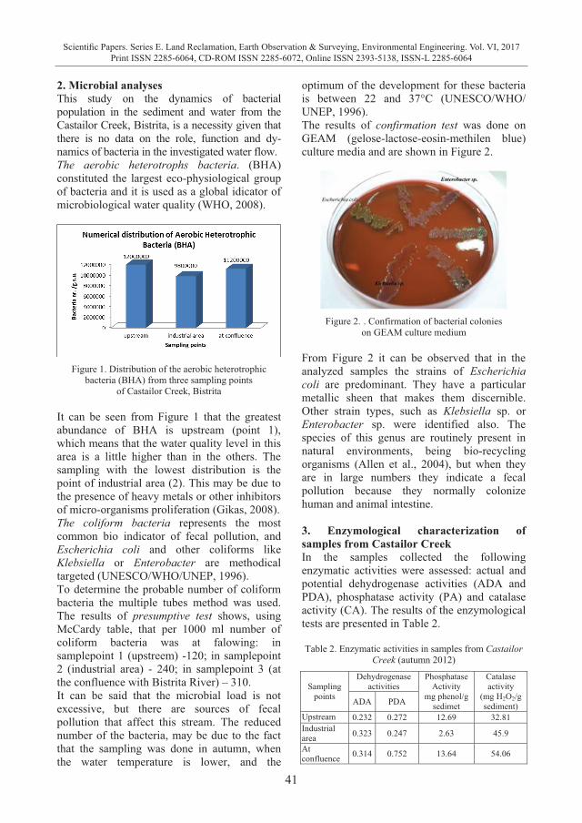
41
Scientific Papers. Series E. Land Reclamation, Earth Observation & Surveying, Environmental Engineering. Vol. VI, 2017Print ISSN 2285-6064, CD-ROM ISSN 2285-6072, Online ISSN 2393-5138, ISSN-L 2285-6064
2. Microbial analyses This study on the dynamics of bacterial population in the sediment and water from the Castailor Creek, Bistrita, is a necessity given that there is no data on the role, function and dy-namics of bacteria in the investigated water flow. The aerobic heterotrophs bacteria. (BHA) constituted the largest eco-physiological group of bacteria and it is used as a global idicator of microbiological water quality (WHO, 2008).
Figure 1. Distribution of the aerobic heterotrophic bacteria (BHA) from three sampling points
of Castailor Creek, Bistrita It can be seen from Figure 1 that the greatest abundance of BHA is upstream (point 1), which means that the water quality level in this area is a little higher than in the others. The sampling with the lowest distribution is the point of industrial area (2). This may be due to the presence of heavy metals or other inhibitors of micro-organisms proliferation (Gikas, 2008). The coliform bacteria represents the most common bio indicator of fecal pollution, and Escherichia coli and other coliforms like Klebsiella or Enterobacter are methodical targeted (UNESCO/WHO/UNEP, 1996). To determine the probable number of coliform bacteria the multiple tubes method was used. The results of presumptive test shows, using McCardy table, that per 1000 ml number of coliform bacteria was at falowing: in samplepoint 1 (upstreem) -120; in samplepoint 2 (industrial area) - 240; in samplepoint 3 (at the confluence with Bistrita River) – 310. It can be said that the microbial load is not excessive, but there are sources of fecal pollution that affect this stream. The reduced number of the bacteria, may be due to the fact that the sampling was done in autumn, when the water temperature is lower, and the
optimum of the development for these bacteria is between 22 and 37°C (UNESCO/WHO/ UNEP, 1996). The results of confirmation test was done on GEAM (gelose-lactose-eosin-methilen blue) culture media and are shown in Figure 2.
Figure 2. . Confirmation of bacterial colonies
on GEAM culture medium
From Figure 2 it can be observed that in the analyzed samples the strains of Escherichia coli are predominant. They have a particular metallic sheen that makes them discernible. Other strain types, such as Klebsiella sp. or Enterobacter sp. were identified also. The species of this genus are routinely present in natural environments, being bio-recycling organisms (Allen et al., 2004), but when they are in large numbers they indicate a fecal pollution because they normally colonize human and animal intestine. 3. Enzymological characterization of samples from Castailor Creek In the samples collected the following enzymatic activities were assessed: actual and potential dehydrogenase activities (ADA and PDA), phosphatase activity (PA) and catalase activity (CA). The results of the enzymological tests are presented in Table 2. Table 2. Enzymatic activities in samples from Castailor
Creek (autumn 2012)
Sampling points
Dehydrogenase activities
Phosphatase Activity
mg phenol/g sedimet
Catalase activity
(mg H2O2/g sediment) ADA PDA
Upstream 0.232 0.272 12.69 32.81Industrial area 0.323 0.247 2.63 45.9
At confluence 0.314 0.752 13.64 54.06
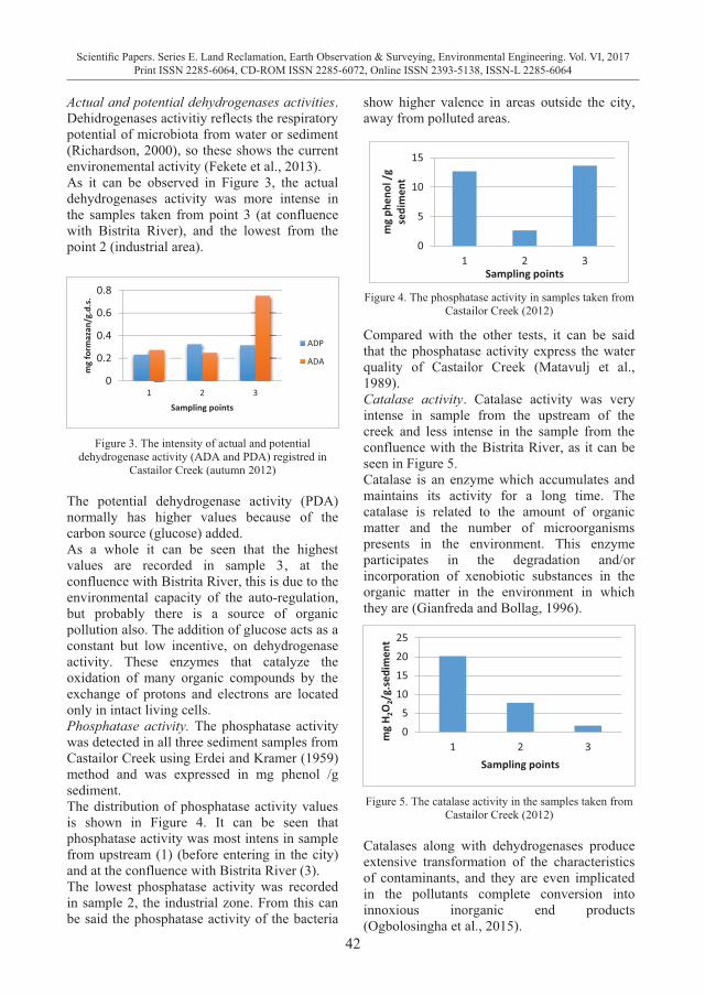
42
Scientific Papers. Series E. Land Reclamation, Earth Observation & Surveying, Environmental Engineering. Vol. VI, 2017Print ISSN 2285-6064, CD-ROM ISSN 2285-6072, Online ISSN 2393-5138, ISSN-L 2285-6064
Actual and potential dehydrogenases activities. Dehidrogenases activitiy reflects the respiratory potential of microbiota from water or sediment (Richardson, 2000), so these shows the current environemental activity (Fekete et al., 2013). As it can be observed in Figure 3, the actual dehydrogenases activity was more intense in the samples taken from point 3 (at confluence with Bistrita River), and the lowest from the point 2 (industrial area).
Figure 3. The intensity of actual and potential
dehydrogenase activity (ADA and PDA) registred in Castailor Creek (autumn 2012)
The potential dehydrogenase activity (PDA) normally has higher values because of the carbon source (glucose) added. As a whole it can be seen that the highest values are recorded in sample 3‚ at the confluence with Bistrita River, this is due to the environmental capacity of the auto-regulation, but probably there is a source of organic pollution also. The addition of glucose acts as a constant but low incentive, on dehydrogenase activity. These enzymes that catalyze the oxidation of many organic compounds by the exchange of protons and electrons are located only in intact living cells. Phosphatase activity. The phosphatase activity was detected in all three sediment samples from Castailor Creek using Erdei and Kramer (1959) method and was expressed in mg phenol /g sediment. The distribution of phosphatase activity values is shown in Figure 4. It can be seen that phosphatase activity was most intens in sample from upstream (1) (before entering in the city) and at the confluence with Bistrita River (3). The lowest phosphatase activity was recorded in sample 2, the industrial zone. From this can be said the phosphatase activity of the bacteria
show higher valence in areas outside the city, away from polluted areas.
Figure 4. The phosphatase activity in samples taken from
Castailor Creek (2012) Compared with the other tests, it can be said that the phosphatase activity express the water quality of Castailor Creek (Matavulj et al., 1989). Catalase activity. Catalase activity was very intense in sample from the upstream of the creek and less intense in the sample from the confluence with the Bistrita River, as it can be seen in Figure 5. Catalase is an enzyme which accumulates and maintains its activity for a long time. The catalase is related to the amount of organic matter and the number of microorganisms presents in the environment. This enzyme participates in the degradation and/or incorporation of xenobiotic substances in the organic matter in the environment in which they are (Gianfreda and Bollag, 1996).
Figure 5. The catalase activity in the samples taken from
Castailor Creek (2012) Catalases along with dehydrogenases produce extensive transformation of the characteristics of contaminants, and they are even implicated in the pollutants complete conversion into innoxious inorganic end products (Ogbolosingha et al., 2015).
0
0.2
0.4
0.6
0.8
1 2 3
mg
form
azan
/g.d
.s.
Sampling points
ADP
ADA
0
5
10
15
1 2 3
mg p
heno
l /g
sedi
men
t
Sampling points
0
5
10
15
20
25
1 2 3
mg H
2O2/
g.se
dim
ent
Sampling points
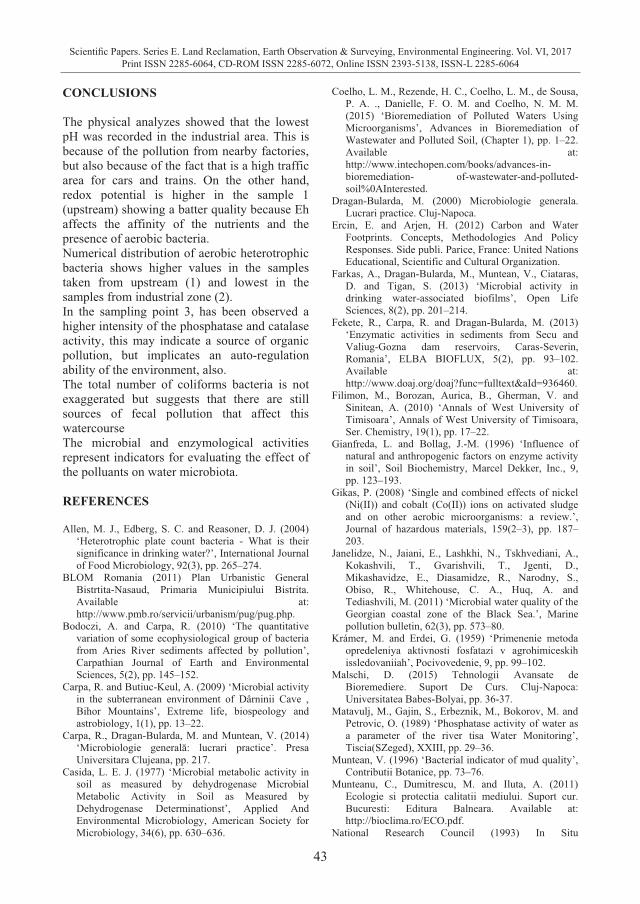
43
Scientific Papers. Series E. Land Reclamation, Earth Observation & Surveying, Environmental Engineering. Vol. VI, 2017Print ISSN 2285-6064, CD-ROM ISSN 2285-6072, Online ISSN 2393-5138, ISSN-L 2285-6064
CONCLUSIONS The physical analyzes showed that the lowest pH was recorded in the industrial area. This is because of the pollution from nearby factories, but also because of the fact that is a high traffic area for cars and trains. On the other hand, redox potential is higher in the sample 1 (upstream) showing a batter quality because Eh affects the affinity of the nutrients and the presence of aerobic bacteria. Numerical distribution of aerobic heterotrophic bacteria shows higher values in the samples taken from upstream (1) and lowest in the samples from industrial zone (2). In the sampling point 3, has been observed a higher intensity of the phosphatase and catalase activity, this may indicate a source of organic pollution, but implicates an auto-regulation ability of the environment, also. The total number of coliforms bacteria is not exaggerated but suggests that there are still sources of fecal pollution that affect this watercourse The microbial and enzymological activities represent indicators for evaluating the effect of the polluants on water microbiota. REFERENCES Allen, M. J., Edberg, S. C. and Reasoner, D. J. (2004)
‘Heterotrophic plate count bacteria - What is their significance in drinking water?’, International Journal of Food Microbiology, 92(3), pp. 265–274.
BLOM Romania (2011) Plan Urbanistic General Bistrtita-Nasaud, Primaria Municipiului Bistrita. Available at: http://www.pmb.ro/servicii/urbanism/pug/pug.php.
Bodoczi, A. and Carpa, R. (2010) ‘The quantitative variation of some ecophysiological group of bacteria from Aries River sediments affected by pollution’, Carpathian Journal of Earth and Environmental Sciences, 5(2), pp. 145–152.
Carpa, R. and Butiuc-Keul, A. (2009) ‘Microbial activity in the subterranean environment of Dârninii Cave , Bihor Mountains’, Extreme life, biospeology and astrobiology, 1(1), pp. 13–22.
Carpa, R., Dragan-Bularda, M. and Muntean, V. (2014) ‘Microbiologie generală: lucrari practice’. Presa Universitara Clujeana, pp. 217.
Casida, L. E. J. (1977) ‘Microbial metabolic activity in soil as measured by dehydrogenase Microbial Metabolic Activity in Soil as Measured by Dehydrogenase Determinationst’, Applied And Environmental Microbiology, American Society for Microbiology, 34(6), pp. 630–636.
Coelho, L. M., Rezende, H. C., Coelho, L. M., de Sousa, P. A. ., Danielle, F. O. M. and Coelho, N. M. M. (2015) ‘Bioremediation of Polluted Waters Using Microorganisms’, Advances in Bioremediation of Wastewater and Polluted Soil, (Chapter 1), pp. 1–22. Available at: http://www.intechopen.com/books/advances-in-bioremediation- of-wastewater-and-polluted-soil%0AInterested.
Dragan-Bularda, M. (2000) Microbiologie generala. Lucrari practice. Cluj-Napoca.
Ercin, E. and Arjen, H. (2012) Carbon and Water Footprints. Concepts, Methodologies And Policy Responses. Side publi. Parice, France: United Nations Educational, Scientific and Cultural Organization.
Farkas, A., Dragan-Bularda, M., Muntean, V., Ciataras, D. and Tigan, S. (2013) ‘Microbial activity in drinking water-associated biofilms’, Open Life Sciences, 8(2), pp. 201–214.
Fekete, R., Carpa, R. and Dragan-Bularda, M. (2013) ‘Enzymatic activities in sediments from Secu and Valiug-Gozna dam reservoirs, Caras-Severin, Romania’, ELBA BIOFLUX, 5(2), pp. 93–102. Available at: http://www.doaj.org/doaj?func=fulltext&aId=936460.
Filimon, M., Borozan, Aurica, B., Gherman, V. and Sinitean, A. (2010) ‘Annals of West University of Timisoara’, Annals of West University of Timisoara, Ser. Chemistry, 19(1), pp. 17–22.
Gianfreda, L. and Bollag, J.-M. (1996) ‘Influence of natural and anthropogenic factors on enzyme activity in soil’, Soil Biochemistry, Marcel Dekker, Inc., 9, pp. 123–193.
Gikas, P. (2008) ‘Single and combined effects of nickel (Ni(II)) and cobalt (Co(II)) ions on activated sludge and on other aerobic microorganisms: a review.’, Journal of hazardous materials, 159(2–3), pp. 187–203.
Janelidze, N., Jaiani, E., Lashkhi, N., Tskhvediani, A., Kokashvili, T., Gvarishvili, T., Jgenti, D., Mikashavidze, E., Diasamidze, R., Narodny, S., Obiso, R., Whitehouse, C. A., Huq, A. and Tediashvili, M. (2011) ‘Microbial water quality of the Georgian coastal zone of the Black Sea.’, Marine pollution bulletin, 62(3), pp. 573–80.
Krámer, M. and Erdei, G. (1959) ‘Primenenie metoda opredeleniya aktivnosti fosfatazi v agrohimiceskih issledovaniiah’, Pocivovedenie, 9, pp. 99–102.
Malschi, D. (2015) Tehnologii Avansate de Bioremediere. Suport De Curs. Cluj-Napoca: Universitatea Babes-Bolyai, pp. 36-37.
Matavulj, M., Gajin, S., Erbeznik, M., Bokorov, M. and Petrovic, O. (1989) ‘Phosphatase activity of water as a parameter of the river tisa Water Monitoring’, Tiscia(SZeged), XXIII, pp. 29–36.
Muntean, V. (1996) ‘Bacterial indicator of mud quality’, Contributii Botanice, pp. 73–76.
Munteanu, C., Dumitrescu, M. and Iluta, A. (2011) Ecologie si protectia calitatii mediului. Suport cur. Bucuresti: Editura Balneara. Available at: http://bioclima.ro/ECO.pdf.
National Research Council (1993) In Situ
44
Scientific Papers. Series E. Land Reclamation, Earth Observation & Surveying, Environmental Engineering. Vol. VI, 2017Print ISSN 2285-6064, CD-ROM ISSN 2285-6072, Online ISSN 2393-5138, ISSN-L 2285-6064
Bioremediation: When Does it Work? Edited by B. E. (Chair) (Committee O. I. S. B. Rittmann. National Academy Press. Available at: http://www.nap.edu/catalog/2131/in-situ-bioremediation-when-does-it-work.
Ogbolosingha, A. J., Essien, E. B. and Ohiri, R. C. (2015) ‘Variation of Lipase , Catalase and Dehydrogenase Activities during Bioremediation of Crude Oil Polluted Soil .’, 5(14), pp. 128–142.
Orban, M. G., Carpa, R. and Dragan, M. (2010) ‘Microbiological and enzymological Research’, Studii şi cercetari, Biology, 16, pp. 45–57.
Pander, J. and Geist, J. (2013) ‘Ecological indicators for stream restoration success’, Ecological Indicators. Elsevier Ltd, 30, pp. 106–118. doi: 10.1016/j.ecolind.2013.01.039.
Qian, F., Dixon, D. R., Newcombe, G., Ho, L., Dreyfus, J. and Scales, P. J. (2014) ‘The effect of pH on the release of metabolites by cyanobacteria in conventional water treatment processes’, Harmful Algae. Elsevier B.V., 39, pp. 253–258. doi: 10.1016/j.hal.2014.08.006.
Richardson, D. J. (2000) ‘Bacterial respiration: A flexibe process for a changing environment’, Microbiology, 146(2000), pp. 551–571. doi: so.
Ríos, F., Lechuga, M., Fernández-Serrano, M. and Fernández-Arteaga, A. (2017) ‘Aerobic
biodegradation of amphoteric amine-oxide-based surfactants: Effect of molecular structure, initial surfactant concentration and pH’, Chemosphere, 171, pp. 324–331.
Suslow, T. V. (2004) ‘Oxidation-Reduction Potential ( ORP ) for Water Disinfection Monitoring , Control , and Documentation’, ANR publication, 8149, pp.1–5. Available at: http://anrcatalog.ucanr.edu/pdf/8149.pdf.
Tillett, H. (1987) ‘Most probable numbers of organisms: revised tables for the multiple tube method’, Epidem. Inf., (99), pp. 471–476. Available at: https://www.ncbi.nlm.nih.gov/pmc/articles/PMC2249285/pdf/epidinfect00005-0237.pdf.
UN-Water (2012) WWDR4: Managing Water under Uncertainty and Risk, The united nations world water development report 4.
UNESCO/WHO/UNEP (1996) Water Quality Assessments - A guide to use of biota, sediments and water in enviromental monitoring, University Press, Cambridge ISBN. Edited by D. Chapman. Cambridge: E&FN Spon, an imprint of Chapman & Hall. doi: 10.4324/9780203476710.
WHO (2008) Guidelines for drinking-water quality. 3rd edn, WHO chronicle. 3rd edn. Edited by B. Gordon, P. Callan, and C. Vickers. Geneva: WHO Library Cataloguing-in-Publication.

45
Scientific Papers. Series E. Land Reclamation, Earth Observation & Surveying, Environmental Engineering. Vol. VI, 2017Print ISSN 2285-6064, CD-ROM ISSN 2285-6072, Online ISSN 2393-5138, ISSN-L 2285-6064
Bioremediation: When Does it Work? Edited by B. E. (Chair) (Committee O. I. S. B. Rittmann. National Academy Press. Available at: http://www.nap.edu/catalog/2131/in-situ-bioremediation-when-does-it-work.
Ogbolosingha, A. J., Essien, E. B. and Ohiri, R. C. (2015) ‘Variation of Lipase , Catalase and Dehydrogenase Activities during Bioremediation of Crude Oil Polluted Soil .’, 5(14), pp. 128–142.
Orban, M. G., Carpa, R. and Dragan, M. (2010) ‘Microbiological and enzymological Research’, Studii şi cercetari, Biology, 16, pp. 45–57.
Pander, J. and Geist, J. (2013) ‘Ecological indicators for stream restoration success’, Ecological Indicators. Elsevier Ltd, 30, pp. 106–118. doi: 10.1016/j.ecolind.2013.01.039.
Qian, F., Dixon, D. R., Newcombe, G., Ho, L., Dreyfus, J. and Scales, P. J. (2014) ‘The effect of pH on the release of metabolites by cyanobacteria in conventional water treatment processes’, Harmful Algae. Elsevier B.V., 39, pp. 253–258. doi: 10.1016/j.hal.2014.08.006.
Richardson, D. J. (2000) ‘Bacterial respiration: A flexibe process for a changing environment’, Microbiology, 146(2000), pp. 551–571. doi: so.
Ríos, F., Lechuga, M., Fernández-Serrano, M. and Fernández-Arteaga, A. (2017) ‘Aerobic
biodegradation of amphoteric amine-oxide-based surfactants: Effect of molecular structure, initial surfactant concentration and pH’, Chemosphere, 171, pp. 324–331.
Suslow, T. V. (2004) ‘Oxidation-Reduction Potential ( ORP ) for Water Disinfection Monitoring , Control , and Documentation’, ANR publication, 8149, pp.1–5. Available at: http://anrcatalog.ucanr.edu/pdf/8149.pdf.
Tillett, H. (1987) ‘Most probable numbers of organisms: revised tables for the multiple tube method’, Epidem. Inf., (99), pp. 471–476. Available at: https://www.ncbi.nlm.nih.gov/pmc/articles/PMC2249285/pdf/epidinfect00005-0237.pdf.
UN-Water (2012) WWDR4: Managing Water under Uncertainty and Risk, The united nations world water development report 4.
UNESCO/WHO/UNEP (1996) Water Quality Assessments - A guide to use of biota, sediments and water in enviromental monitoring, University Press, Cambridge ISBN. Edited by D. Chapman. Cambridge: E&FN Spon, an imprint of Chapman & Hall. doi: 10.4324/9780203476710.
WHO (2008) Guidelines for drinking-water quality. 3rd edn, WHO chronicle. 3rd edn. Edited by B. Gordon, P. Callan, and C. Vickers. Geneva: WHO Library Cataloguing-in-Publication.
ASSESSING THE CONSERVATION STATUS OF FISH SPECIES
FROM THE GILORT RIVER PROTECTED AREA
Irina-Ramona PECINGINA, Roxana-Gabriela POPA
”Constantin Brancusi” University of Targu Jiu, 30 Eroilor Street, Targu Jiu, Gorj, Romania
Corresponding author email: [email protected] Abstract The paper aimed to present the state of conservation of the fish species of community interest (Eudontomyzon mariae, Gobio albipinnatus, Barbus meridionalis, Sabanejewia aurata) in the protected area. For evaluating the conservation status of fish species have been carried out land evaluation in May - October 2014 with a frequency of 3-4 observations per month. Following the site assessments in the Natura 2000 Gilort River area, it was observed that the conservation status of the species Eudontomyzon mariae population is medium to low, highlighting a reduction in population (21 specimens); the conservation status of the species Gobio albipinnatus population is medium to low, highlighting a reduction in population (16 specimens); the conservation status of the species Barbus meridionalis population is good, the population being stable (744 specimens); the conservation status of the species Sabanejewia aurata population is medium to low, highlighting a reduction in population (240 specimens). Key words: assessment, conservation, Natural Protected Area INTRODUCTION The Gilort River protected area is a site of community importance and belongs of the Natura 2000 European network. The purpose of Gilort River protected area is to protect and conserve species of important national and Community level (Lutra lutra, Bombina variegata, Eudontomyzon mariae, Gobio albipinnatus, Barbus meridionalis, Sabanejewia aurata). The reason for designating area Gilort River as protected was due to existence on its territory of the species of relevant community interest for conservation in the biogeographic region they belong. The Gilort River protected area lies in Gorj, in sub-Carpathians Getici, in the Ciolanei Basin and is bordered by the localities: Pociovalistea and Bumbesti-Pițic at north, natural protected area Prigoria-Bengesti and localities Mirosloveni, Albeni, Bolbocesti and Barzeiu de Gilort at east, locality Doseni at south and localities Albeni, Bengesti, Ciocadia and Balcesti at west. The natural protected area develops longitudinally from north to south, with a length of 21.75 km Gilort River (Figure 1).
Figure 1. Localization of the Gilort River natural
protected area The Gilort River protected area is located within the territorial administrative units of Bengesti, Albeni, Novaci, Bumbesti-Pitic si Targu Carbunesti in the Gorj County, including an area of 873 ha (Figure 2).
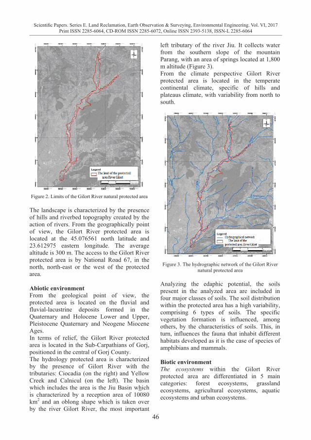
46
Scientific Papers. Series E. Land Reclamation, Earth Observation & Surveying, Environmental Engineering. Vol. VI, 2017Print ISSN 2285-6064, CD-ROM ISSN 2285-6072, Online ISSN 2393-5138, ISSN-L 2285-6064
Figure 2. Limits of the Gilort River natural protected area The landscape is characterized by the presence of hills and riverbed topography created by the action of rivers. From the geographically point of view, the Gilort River protected area is located at the 45.076561 north latitude and 23.612975 eastern longitude. The average altitude is 300 m. The access to the Gilort River protected area is by National Road 67, in the north, north-east or the west of the protected area. Abiotic environment From the geological point of view, the protected area is located on the fluvial and fluvial-lacustrine deposits formed in the Quaternary and Holocene Lower and Upper, Pleistocene Quaternary and Neogene Miocene Ages. In terms of relief, the Gilort River protected area is located in the Sub-Carpathians of Gorj, positioned in the central of Gorj County. The hydrology protected area is characterized by the presence of Gilort River with the tributaries: Ciocadia (on the right) and Yellow Creek and Calnicul (on the left). The basin which includes the area is the Jiu Basin which is characterized by a reception area of 10080 km2 and an oblong shape which is taken over by the river Gilort River, the most important
left tributary of the river Jiu. It collects water from the southern slope of the mountain Parang, with an area of springs located at 1,800 m altitude (Figure 3). From the climate perspective Gilort River protected area is located in the temperate continental climate, specific of hills and plateaus climate, with variability from north to south.
Figure 3. The hydrographic network of the Gilort River
natural protected area Analyzing the edaphic potential, the soils present in the analyzed area are included in four major classes of soils. The soil distribution within the protected area has a high variability, comprising 6 types of soils. The specific vegetation formation is influenced, among others, by the characteristics of soils. This, in turn, influences the fauna that inhabit different habitats developed as it is the case of species of amphibians and mammals. Biotic environment The ecosystems within the Gilort River protected area are differentiated in 5 main categories: forest ecosystems, grassland ecosystems, agricultural ecosystems, aquatic ecosystems and urban ecosystems.
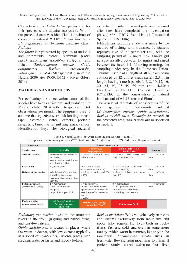
47
Scientific Papers. Series E. Land Reclamation, Earth Observation & Surveying, Environmental Engineering. Vol. VI, 2017Print ISSN 2285-6064, CD-ROM ISSN 2285-6072, Online ISSN 2393-5138, ISSN-L 2285-6064
Characteristic for Lutra Lutra species and for fish species is the aquatic ecosystem. Within the protected area was identified the habitat of community interest 91E0* alluvial forests cu Alnus glutinosa and Fraxinus excelsior (Alno-Padion). The fauna is represented by species of national and community interest: mammals (Lutra lutra), amphibians (Bombina variegata) and fishes (Eudontomyzon mariae, Gobio albipinnatus, Barbus meridionalis, Sabanejewia aurata) (Management plan of the Natura 2000 site ROSCI0362 - River Gilort, 2014) MATERIALS AND METHODS For evaluating the conservation status of fish species have been carried out land evaluation in May - October 2014 with a frequency of 3-4 observations per month. The equipment used to achieve the objective were fish landing, metric tape, electronic scales, camera, portable magnifier, binocular magnifying glass, caliper, identification key. The biological material
extracted in order to investigate was released after they have completed the investigation phase.( ***- IUCN Red List of Threatened Species. IUCN 2006). Ichtyofauna sampling study was made by the method of fishing with trammel, 10 stations representative of the perimeter area, with the sampling period of 12 hours, 18-20 hours gill nets are installed between the nights and raised between the hours 6-8 following morning, the sampling under way in the European Union. Trammel used had a length of 30 m, each being composed of 12 gillnet mesh panels 2.5 m in length, having a mesh panels 6, 6, 8, 10, 12, 16, 20, 24, 30, 35 45, 55 mm (*** Habitats Directive 92/43/EEC. Council Directive 92/43/EEC on the conservation of natural habitats and of wild Fauna and Flora). The assess of the state of conservation of the fish species of community interest (Eudontomyzon mariae, Gobio albipinnatus, Barbus meridionalis, Sabanejewia aurata) in the protected area, was carried out as specified in Table 1.
Table 1. Specifications for evaluating the conservation status of
fish species of community interest (*** Guidelines for Application of IUCN Red List at Regional Levels) Parameters Conservation status
Species code Favorable Unfavorable inappropriate
Unfavorable totally inadequate Unknown
Aria distribution - distribution area stable or increasing; - reduction area distribution with less than 10%
- reduction distribution area with 11-20%
- reduction distribution area with more than 20%
- insufficient data
Population A ≥33 ex./year A = 25-20 ex./year (a decrease of 10- 40%)
A < 13 ex./year (a decrease of more than 40%)
- insufficient data
Habitat of the species - the habitat of the species is stable or increasing; - reduction habitat with less than 5%
- reduction habitat with 6% - 15%
-reduction habitat with more than 15%
- insufficient data
Future prospects (maximum 30 years)
1 = perspectives Good - viability and prosperity of species are provided
2 = perspectives Weak – it is probably that species meet difficulties if conditions of environment are not modified.
3 = perspectives Bad – species under the influence of severe threats its viability is not assured
- insufficient data
Evaluating the conservation status
All "green" or three "green" and one
"unknown"
One or More "orange" but neither "red" One or more "red"
Eudontomyzon mariae lives in the mountain rivers in the trout, grayling and barbel areas, and less downstream. Gobio albipinnatus is locates in places where the water is deeper, with low current (typically at a speed of 28-45 cm/s). Avoids places with stagnant water or faster and muddy bottom.
Barbus meridionalis lives exclusively in rivers and streams exclusively from mountains and upper hilly region; He lives both in rocky rivers, fast and cold, and even in some more muddy, which warm in summer, but only in the mountains. Sabanejewia aurata lives in freshwater flowing from mountains to plains. It prefers sandy gravel substrate but lives
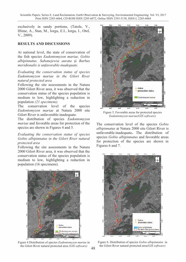
48
Scientific Papers. Series E. Land Reclamation, Earth Observation & Surveying, Environmental Engineering. Vol. VI, 2017Print ISSN 2285-6064, CD-ROM ISSN 2285-6072, Online ISSN 2393-5138, ISSN-L 2285-6064
exclusively in sandy portions, (Tatole, V., Iftime, A., Stan, M., Iorgu, E.I., Iorgu, I., Otel, V., 2009). RESULTS AND DISCUSSIONS At national level, the state of conservation of the fish species Eudontomyzon mariae, Gobio albipinnatus, Sabanejewia aurata și Barbus meridionalis is unfavorable-inadequate. Evaluating the conservation status of species Eudontomyzon mariae in the Gilort River natural protected area Following the site assessments in the Natura 2000 Gilort River area, it was observed that the conservation status of the species population is medium to low, highlighting a reduction in population (21 specimens). The conservation level of the species Eudontomyzon mariae at Natura 2000 site Gilort River is unfavorable-inadequate. The distribution of species Eudontomyzon mariae and favorable areas for protection of the species are shown in Figures 4 and 5. Evaluating the conservation status of species Gobio albipinnatus in the Gilort River natural protected area Following the site assessments in the Natura 2000 Gilort River area, it was observed that the conservation status of the species population is medium to low, highlighting a reduction in population (16 specimens).
Figure 4 Distribution of species Eudontomyzon mariae in
the Gilort River natural protected area (GIS software)
Figure 5. Favorable areas for protected species
Eudontomyzon mariae(GIS software) The conservation level of the species Gobio albipinnatus at Natura 2000 site Gilort River is unfavorable-inadequate. The distribution of species Gobio albipinnatus and favorable areas for protection of the species are shown in Figures 6 and 7.
Figure 6. Distribution of species Gobio albipinnatus in
the Gilort River natural protected area(GIS software)
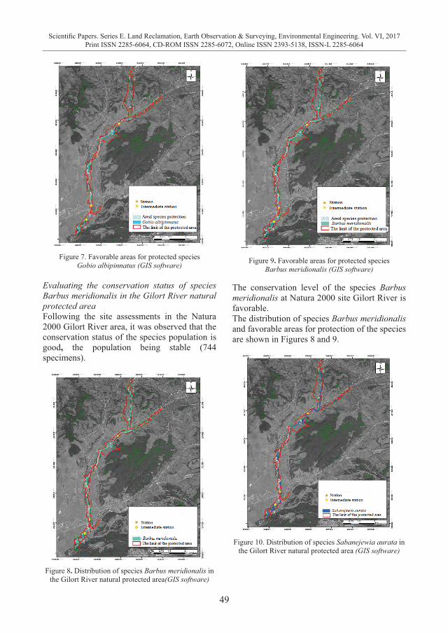
49
Scientific Papers. Series E. Land Reclamation, Earth Observation & Surveying, Environmental Engineering. Vol. VI, 2017Print ISSN 2285-6064, CD-ROM ISSN 2285-6072, Online ISSN 2393-5138, ISSN-L 2285-6064
exclusively in sandy portions, (Tatole, V., Iftime, A., Stan, M., Iorgu, E.I., Iorgu, I., Otel, V., 2009). RESULTS AND DISCUSSIONS At national level, the state of conservation of the fish species Eudontomyzon mariae, Gobio albipinnatus, Sabanejewia aurata și Barbus meridionalis is unfavorable-inadequate. Evaluating the conservation status of species Eudontomyzon mariae in the Gilort River natural protected area Following the site assessments in the Natura 2000 Gilort River area, it was observed that the conservation status of the species population is medium to low, highlighting a reduction in population (21 specimens). The conservation level of the species Eudontomyzon mariae at Natura 2000 site Gilort River is unfavorable-inadequate. The distribution of species Eudontomyzon mariae and favorable areas for protection of the species are shown in Figures 4 and 5. Evaluating the conservation status of species Gobio albipinnatus in the Gilort River natural protected area Following the site assessments in the Natura 2000 Gilort River area, it was observed that the conservation status of the species population is medium to low, highlighting a reduction in population (16 specimens).
Figure 4 Distribution of species Eudontomyzon mariae in
the Gilort River natural protected area (GIS software)
Figure 5. Favorable areas for protected species
Eudontomyzon mariae(GIS software) The conservation level of the species Gobio albipinnatus at Natura 2000 site Gilort River is unfavorable-inadequate. The distribution of species Gobio albipinnatus and favorable areas for protection of the species are shown in Figures 6 and 7.
Figure 6. Distribution of species Gobio albipinnatus in
the Gilort River natural protected area(GIS software)
Figure 7. Favorable areas for protected species
Gobio albipinnatus (GIS software) Evaluating the conservation status of species Barbus meridionalis in the Gilort River natural protected area Following the site assessments in the Natura 2000 Gilort River area, it was observed that the conservation status of the species population is good, the population being stable (744 specimens).
Figure 8. Distribution of species Barbus meridionalis in
the Gilort River natural protected area(GIS software)
Figure 9. Favorable areas for protected species
Barbus meridionalis (GIS software)
The conservation level of the species Barbus meridionalis at Natura 2000 site Gilort River is favorable. The distribution of species Barbus meridionalis and favorable areas for protection of the species are shown in Figures 8 and 9.
Figure 10. Distribution of species Sabanejewia aurata in
the Gilort River natural protected area (GIS software)
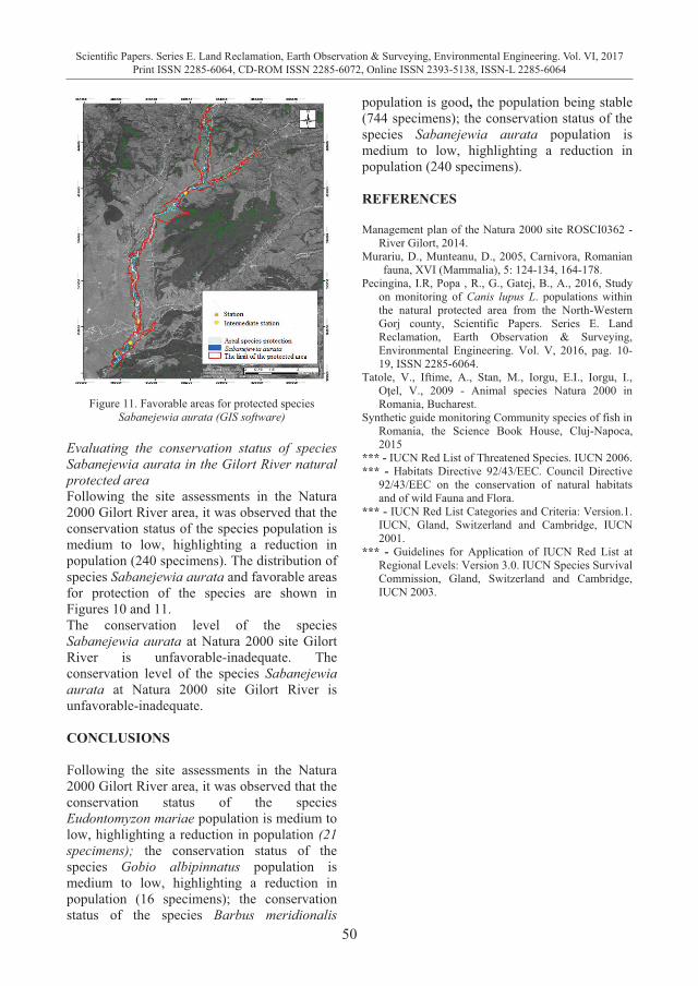
50
Scientific Papers. Series E. Land Reclamation, Earth Observation & Surveying, Environmental Engineering. Vol. VI, 2017Print ISSN 2285-6064, CD-ROM ISSN 2285-6072, Online ISSN 2393-5138, ISSN-L 2285-6064
Figure 11. Favorable areas for protected species
Sabanejewia aurata (GIS software)
Evaluating the conservation status of species Sabanejewia aurata in the Gilort River natural protected area Following the site assessments in the Natura 2000 Gilort River area, it was observed that the conservation status of the species population is medium to low, highlighting a reduction in population (240 specimens). The distribution of species Sabanejewia aurata and favorable areas for protection of the species are shown in Figures 10 and 11. The conservation level of the species Sabanejewia aurata at Natura 2000 site Gilort River is unfavorable-inadequate. The conservation level of the species Sabanejewia aurata at Natura 2000 site Gilort River is unfavorable-inadequate. CONCLUSIONS Following the site assessments in the Natura 2000 Gilort River area, it was observed that the conservation status of the species Eudontomyzon mariae population is medium to low, highlighting a reduction in population (21 specimens); the conservation status of the species Gobio albipinnatus population is medium to low, highlighting a reduction in population (16 specimens); the conservation status of the species Barbus meridionalis
population is good, the population being stable (744 specimens); the conservation status of the species Sabanejewia aurata population is medium to low, highlighting a reduction in population (240 specimens). REFERENCES Management plan of the Natura 2000 site ROSCI0362 -
River Gilort, 2014. Murariu, D., Munteanu, D., 2005, Carnivora, Romanian
fauna, XVI (Mammalia), 5: 124-134, 164-178. Pecingina, I.R, Popa , R., G., Gatej, B., A., 2016, Study
on monitoring of Canis lupus L. populations within the natural protected area from the North-Western Gorj county, Scientific Papers. Series E. Land Reclamation, Earth Observation & Surveying, Environmental Engineering. Vol. V, 2016, pag. 10-19, ISSN 2285-6064.
Tatole, V., Iftime, A., Stan, M., Iorgu, E.I., Iorgu, I., Oţel, V., 2009 - Animal species Natura 2000 in Romania, Bucharest.
Synthetic guide monitoring Community species of fish in Romania, the Science Book House, Cluj-Napoca, 2015
*** - IUCN Red List of Threatened Species. IUCN 2006. *** - Habitats Directive 92/43/EEC. Council Directive
92/43/EEC on the conservation of natural habitats and of wild Fauna and Flora.
*** - IUCN Red List Categories and Criteria: Version.1. IUCN, Gland, Switzerland and Cambridge, IUCN 2001.
*** - Guidelines for Application of IUCN Red List at Regional Levels: Version 3.0. IUCN Species Survival Commission, Gland, Switzerland and Cambridge, IUCN 2003.
51
Scientific Papers. Series E. Land Reclamation, Earth Observation & Surveying, Environmental Engineering. Vol. VI, 2017Print ISSN 2285-6064, CD-ROM ISSN 2285-6072, Online ISSN 2393-5138, ISSN-L 2285-6064
Figure 11. Favorable areas for protected species
Sabanejewia aurata (GIS software)
Evaluating the conservation status of species Sabanejewia aurata in the Gilort River natural protected area Following the site assessments in the Natura 2000 Gilort River area, it was observed that the conservation status of the species population is medium to low, highlighting a reduction in population (240 specimens). The distribution of species Sabanejewia aurata and favorable areas for protection of the species are shown in Figures 10 and 11. The conservation level of the species Sabanejewia aurata at Natura 2000 site Gilort River is unfavorable-inadequate. The conservation level of the species Sabanejewia aurata at Natura 2000 site Gilort River is unfavorable-inadequate. CONCLUSIONS Following the site assessments in the Natura 2000 Gilort River area, it was observed that the conservation status of the species Eudontomyzon mariae population is medium to low, highlighting a reduction in population (21 specimens); the conservation status of the species Gobio albipinnatus population is medium to low, highlighting a reduction in population (16 specimens); the conservation status of the species Barbus meridionalis
population is good, the population being stable (744 specimens); the conservation status of the species Sabanejewia aurata population is medium to low, highlighting a reduction in population (240 specimens). REFERENCES Management plan of the Natura 2000 site ROSCI0362 -
River Gilort, 2014. Murariu, D., Munteanu, D., 2005, Carnivora, Romanian
fauna, XVI (Mammalia), 5: 124-134, 164-178. Pecingina, I.R, Popa , R., G., Gatej, B., A., 2016, Study
on monitoring of Canis lupus L. populations within the natural protected area from the North-Western Gorj county, Scientific Papers. Series E. Land Reclamation, Earth Observation & Surveying, Environmental Engineering. Vol. V, 2016, pag. 10-19, ISSN 2285-6064.
Tatole, V., Iftime, A., Stan, M., Iorgu, E.I., Iorgu, I., Oţel, V., 2009 - Animal species Natura 2000 in Romania, Bucharest.
Synthetic guide monitoring Community species of fish in Romania, the Science Book House, Cluj-Napoca, 2015
*** - IUCN Red List of Threatened Species. IUCN 2006. *** - Habitats Directive 92/43/EEC. Council Directive
92/43/EEC on the conservation of natural habitats and of wild Fauna and Flora.
*** - IUCN Red List Categories and Criteria: Version.1. IUCN, Gland, Switzerland and Cambridge, IUCN 2001.
*** - Guidelines for Application of IUCN Red List at Regional Levels: Version 3.0. IUCN Species Survival Commission, Gland, Switzerland and Cambridge, IUCN 2003.
PHYSICAL-CHEMICAL PROPERTIES ANALYSIS OF THE SOIL
CONTAMINATED WITH HEAVY METALS FROM COPSA MICA AREA
Ioana Monica SUR1, Alexandra CIMPEAN1, Valer MICLE1, Claudiu TANASELIA2
1Technical University of Cluj–Napoca, 103–105 Muncii Blvd., 400641, Cluj–Napoca, Romania 2INCDO-INOE 2000 ICIA, Cluj–Napoca, 67 Donath St., Cluj–Napoca, Romania
Corresponding author email: [email protected]
Abstract The non-ferrous metallurgical activities led to the pollution of large areas of soil and affected the environment in a negative way. The problems generated by soil contamination with different pollutant substances have been, in the latest period in the center of attention for researchers from all around the world. The objective of this paper is to perform experimental researches in order to establish the physical-chemical properties of the soil from Copsa Mica area. The texture, structure, humidity and pH are the main analysis performed in order to proper establish the optimal soil cleaning technologies. In order to establish the actual pollution degree in the moment of soil sampling, was determined also the concentration of metals in the soil. For this purpose, were taken soil samples from two areas on three depth interval (0–40 cm). Determining the concentration of heavy metals on three depth levels offers the researcher a relevant view of the historical pollution of the area under study. As a result of these researches was established that the soil is polluted with Pb, Zn and Cd. The quantity on metals in the soil is way beyond the alert threshold. As a conclusion these soil need cleaning, which can be made through various methods, one of the being bioleaching, which is a biological cleaning method which implies using microorganisms in order to favor leaching and heavy metals extraction from the polluted soils. Key words: Copsa Mica, heavy metals, polluted soil, physical-chemical properties INTRODUCTION Environment pollution is considered to be the most dangerous and constant global threat. The pollutant agents from the environment have a significant impact on the ecosystems and induce an unbalance between the environment, human component and non-human. This unbalance leads to negative effects on all life forms (Morarescu, 2014). In Romania, intensified industrial metallurgical activity in the last 150 years has led to pollution, with aggressive and very powerful effects on the soil, especially due to the presence of heavy metals in the soil but also in the sub terrain water system, the most frequent metals being copper, lead, zinc and cadmium. The most contaminated areas in the country are Baia Mare, Copsa Mica and Zlatna (Botnariuc and Vadineanu, 1982). The concentrations of metals from this area were studied in order to evaluate the pollution degree. The findings from 2010 highlighted high concentrations of metals near the deposits: Zn: 416 mg/kg; Pb: 284 mg/kg; Cd: 0.9 mg/kg; (Sucuturdean and Micle, 2011).
In 2012 was made a study regarding the concentration of metals from the soil surrounding the company (300 m) from different depths: Cu: 466-123.8 mg/kg; Cd: 15.8-31.4 mg/kg; Zn: 447-543 mg/kg; Pb: 148-739 mg/kg (Maria Szanto Prodan et. al., 2012). Bioleaching, or bacterial leaching, consists in the extraction by solubilization of the metallic elements from contaminated soil using bacteria. This method does not destroy (eliminate) the pollutants, but it favors their segregation from the contaminated environment, due to the fact that the microorganisms have the property to oxidize, transforming the pollutants into sulfates with a more soluble form or ferric compounds (Gadd, 2004; Liu et. al., 2008 ). Microorganisms or bacteria used in bioleaching process oxidize directly or indirectly inorganic compounds (Jayesh et. al., 2007). In direct process, bacteria can directly oxidize sulphur ion in sulphate from metal sulphide (Chen et. al., 2004; Liu et. al., 2008; Jayesh et. al., 2007). Using the indirect process, oxidation of metal sulphides is generated in microbial way by ferric ions (Jayesh et. al., 2007).
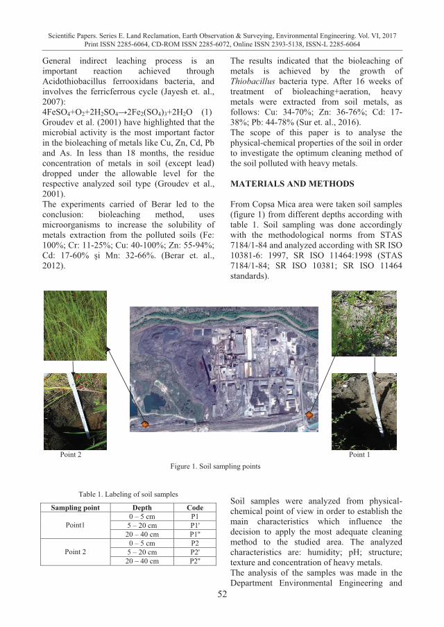
52
Scientific Papers. Series E. Land Reclamation, Earth Observation & Surveying, Environmental Engineering. Vol. VI, 2017Print ISSN 2285-6064, CD-ROM ISSN 2285-6072, Online ISSN 2393-5138, ISSN-L 2285-6064
General indirect leaching process is an important reaction achieved through Acidothiobacillus ferrooxidans bacteria, and involves the ferricferrous cycle (Jayesh et. al., 2007): 4FeSO4+O2+2H2SO4→2Fe2(SO4)3+2H2O (1) Groudev et al. (2001) have highlighted that the microbial activity is the most important factor in the bioleaching of metals like Cu, Zn, Cd, Pb and As. In less than 18 months, the residue concentration of metals in soil (except lead) dropped under the allowable level for the respective analyzed soil type (Groudev et al., 2001). The experiments carried of Berar led to the conclusion: bioleaching method, uses microorganisms to increase the solubility of metals extraction from the polluted soils (Fe: 100%; Cr: 11-25%; Cu: 40-100%; Zn: 55-94%; Cd: 17-60% și Mn: 32-66%. (Berar et. al., 2012).
The results indicated that the bioleaching of metals is achieved by the growth of Thiobacillus bacteria type. After 16 weeks of treatment of bioleaching+aeration, heavy metals were extracted from soil metals, as follows: Cu: 34-70%; Zn: 36-76%; Cd: 17-38%; Pb: 44-78% (Sur et. al., 2016). The scope of this paper is to analyse the physical-chemical properties of the soil in order to investigate the optimum cleaning method of the soil polluted with heavy metals. MATERIALS AND METHODS From Copsa Mica area were taken soil samples (figure 1) from different depths according with table 1. Soil sampling was done accordingly with the methodological norms from STAS 7184/1-84 and analyzed according with SR ISO 10381-6: 1997, SR ISO 11464:1998 (STAS 7184/1-84; SR ISO 10381; SR ISO 11464 standards).
Point 2 Point 1 Figure 1. Soil sampling points
Table 1. Labeling of soil samples
Sampling point Depth Code
Point1 0 – 5 cm P1 5 – 20 cm P1'
20 – 40 cm P1''
Point 2 0 – 5 cm P2 5 – 20 cm P2'
20 – 40 cm P2''
Soil samples were analyzed from physical-chemical point of view in order to establish the main characteristics which influence the decision to apply the most adequate cleaning method to the studied area. The analyzed characteristics are: humidity; pH; structure; texture and concentration of heavy metals. The analysis of the samples was made in the Department Environmental Engineering and
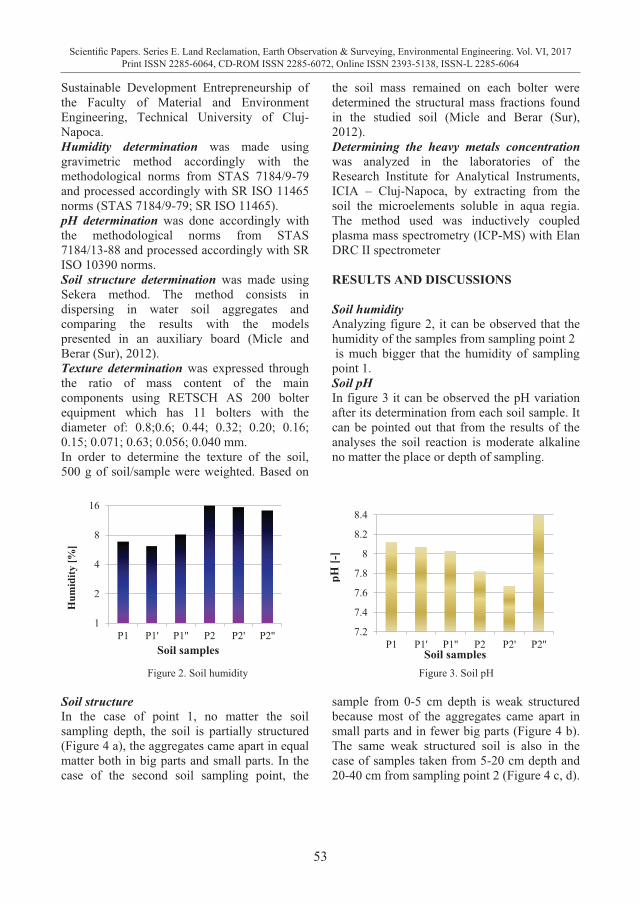
53
Scientific Papers. Series E. Land Reclamation, Earth Observation & Surveying, Environmental Engineering. Vol. VI, 2017Print ISSN 2285-6064, CD-ROM ISSN 2285-6072, Online ISSN 2393-5138, ISSN-L 2285-6064
General indirect leaching process is an important reaction achieved through Acidothiobacillus ferrooxidans bacteria, and involves the ferricferrous cycle (Jayesh et. al., 2007): 4FeSO4+O2+2H2SO4→2Fe2(SO4)3+2H2O (1) Groudev et al. (2001) have highlighted that the microbial activity is the most important factor in the bioleaching of metals like Cu, Zn, Cd, Pb and As. In less than 18 months, the residue concentration of metals in soil (except lead) dropped under the allowable level for the respective analyzed soil type (Groudev et al., 2001). The experiments carried of Berar led to the conclusion: bioleaching method, uses microorganisms to increase the solubility of metals extraction from the polluted soils (Fe: 100%; Cr: 11-25%; Cu: 40-100%; Zn: 55-94%; Cd: 17-60% și Mn: 32-66%. (Berar et. al., 2012).
The results indicated that the bioleaching of metals is achieved by the growth of Thiobacillus bacteria type. After 16 weeks of treatment of bioleaching+aeration, heavy metals were extracted from soil metals, as follows: Cu: 34-70%; Zn: 36-76%; Cd: 17-38%; Pb: 44-78% (Sur et. al., 2016). The scope of this paper is to analyse the physical-chemical properties of the soil in order to investigate the optimum cleaning method of the soil polluted with heavy metals. MATERIALS AND METHODS From Copsa Mica area were taken soil samples (figure 1) from different depths according with table 1. Soil sampling was done accordingly with the methodological norms from STAS 7184/1-84 and analyzed according with SR ISO 10381-6: 1997, SR ISO 11464:1998 (STAS 7184/1-84; SR ISO 10381; SR ISO 11464 standards).
Point 2 Point 1 Figure 1. Soil sampling points
Table 1. Labeling of soil samples
Sampling point Depth Code
Point1 0 – 5 cm P1 5 – 20 cm P1'
20 – 40 cm P1''
Point 2 0 – 5 cm P2 5 – 20 cm P2'
20 – 40 cm P2''
Soil samples were analyzed from physical-chemical point of view in order to establish the main characteristics which influence the decision to apply the most adequate cleaning method to the studied area. The analyzed characteristics are: humidity; pH; structure; texture and concentration of heavy metals. The analysis of the samples was made in the Department Environmental Engineering and
Sustainable Development Entrepreneurship of the Faculty of Material and Environment Engineering, Technical University of Cluj-Napoca. Humidity determination was made using gravimetric method accordingly with the methodological norms from STAS 7184/9-79 and processed accordingly with SR ISO 11465 norms (STAS 7184/9-79; SR ISO 11465). pH determination was done accordingly with the methodological norms from STAS 7184/13-88 and processed accordingly with SR ISO 10390 norms. Soil structure determination was made using Sekera method. The method consists in dispersing in water soil aggregates and comparing the results with the models presented in an auxiliary board (Micle and Berar (Sur), 2012). Texture determination was expressed through the ratio of mass content of the main components using RETSCH AS 200 bolter equipment which has 11 bolters with the diameter of: 0.8;0.6; 0.44; 0.32; 0.20; 0.16; 0.15; 0.071; 0.63; 0.056; 0.040 mm. In order to determine the texture of the soil, 500 g of soil/sample were weighted. Based on
the soil mass remained on each bolter were determined the structural mass fractions found in the studied soil (Micle and Berar (Sur), 2012). Determining the heavy metals concentration was analyzed in the laboratories of the Research Institute for Analytical Instruments, ICIA – Cluj-Napoca, by extracting from the soil the microelements soluble in aqua regia. The method used was inductively coupled plasma mass spectrometry (ICP-MS) with Elan DRC II spectrometer RESULTS AND DISCUSSIONS Soil humidity Analyzing figure 2, it can be observed that the humidity of the samples from sampling point 2 is much bigger that the humidity of sampling point 1. Soil pH In figure 3 it can be observed the pH variation after its determination from each soil sample. It can be pointed out that from the results of the analyses the soil reaction is moderate alkaline no matter the place or depth of sampling.
Figure 2. Soil humidity Figure 3. Soil pH
Soil structure In the case of point 1, no matter the soil sampling depth, the soil is partially structured (Figure 4 a), the aggregates came apart in equal matter both in big parts and small parts. In the case of the second soil sampling point, the
sample from 0-5 cm depth is weak structured because most of the aggregates came apart in small parts and in fewer big parts (Figure 4 b). The same weak structured soil is also in the case of samples taken from 5-20 cm depth and 20-40 cm from sampling point 2 (Figure 4 c, d).
1
2
4
8
16
P1 P1' P1'' P2 P2' P2''
Hum
idity
[%]
Soil samples 7.2
7.4
7.6
7.8
8
8.2
8.4
P1 P1' P1'' P2 P2' P2''
pH
[-]
Soil samples
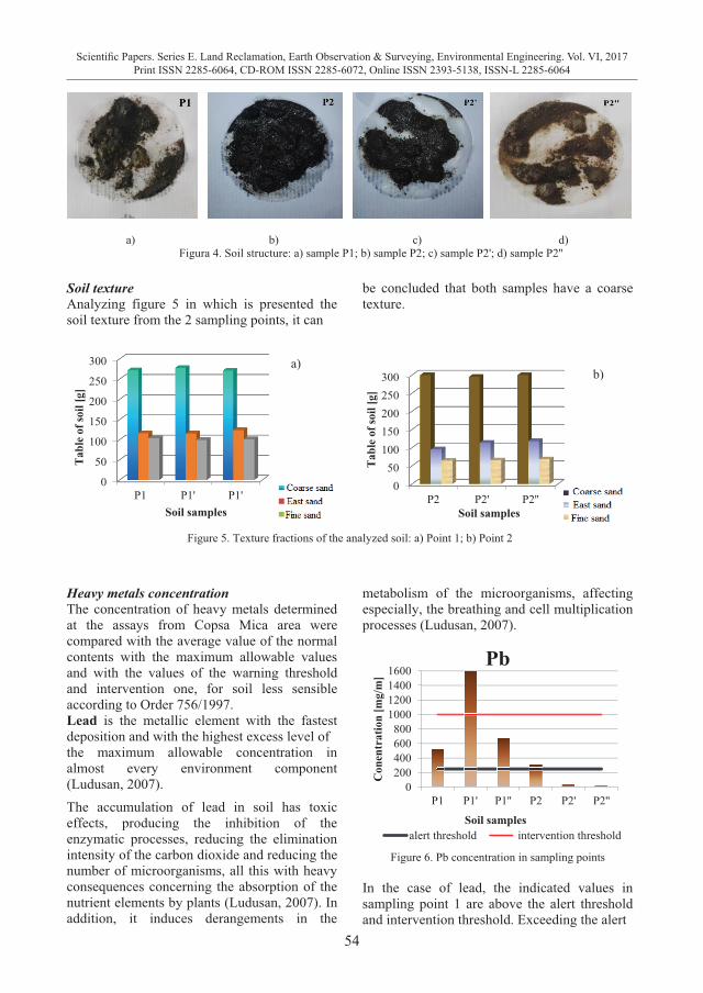
54
Scientific Papers. Series E. Land Reclamation, Earth Observation & Surveying, Environmental Engineering. Vol. VI, 2017Print ISSN 2285-6064, CD-ROM ISSN 2285-6072, Online ISSN 2393-5138, ISSN-L 2285-6064
a) b) c) d) Figura 4. Soil structure: a) sample P1; b) sample P2; c) sample P2'; d) sample P2''
Soil textureAnalyzing figure 5 in which is presented the soil texture from the 2 sampling points, it can
be concluded that both samples have a coarse texture.
Figure 5. Texture fractions of the analyzed soil: a) Point 1; b) Point 2
Heavy metals concentration The concentration of heavy metals determined at the assays from Copsa Mica area were compared with the average value of the normal contents with the maximum allowable values and with the values of the warning threshold and intervention one, for soil less sensible according to Order 756/1997. Lead is the metallic element with the fastest deposition and with the highest excess level of the maximum allowable concentration in almost every environment component (Ludusan, 2007). The accumulation of lead in soil has toxic effects, producing the inhibition of the enzymatic processes, reducing the elimination intensity of the carbon dioxide and reducing the number of microorganisms, all this with heavy consequences concerning the absorption of the nutrient elements by plants (Ludusan, 2007). In addition, it induces derangements in the
metabolism of the microorganisms, affecting especially, the breathing and cell multiplication processes (Ludusan, 2007).
Figure 6. Pb concentration in sampling points
In the case of lead, the indicated values in sampling point 1 are above the alert threshold and intervention threshold. Exceeding the alert
0
50
100
150
200
250
300
P1 P1' P1'
Tabl
e of
soil
[g]
Soil samples
a)
050
100150200250300
P2 P2' P2''
Tabl
e of
soil
[g]
Soil samples
b)
0200400600800
1000120014001600
P1 P1' P1'' P2 P2' P2''
Con
entr
atio
n [m
g/m
]
Pb
alert threshold intervention thresholdSoil samples
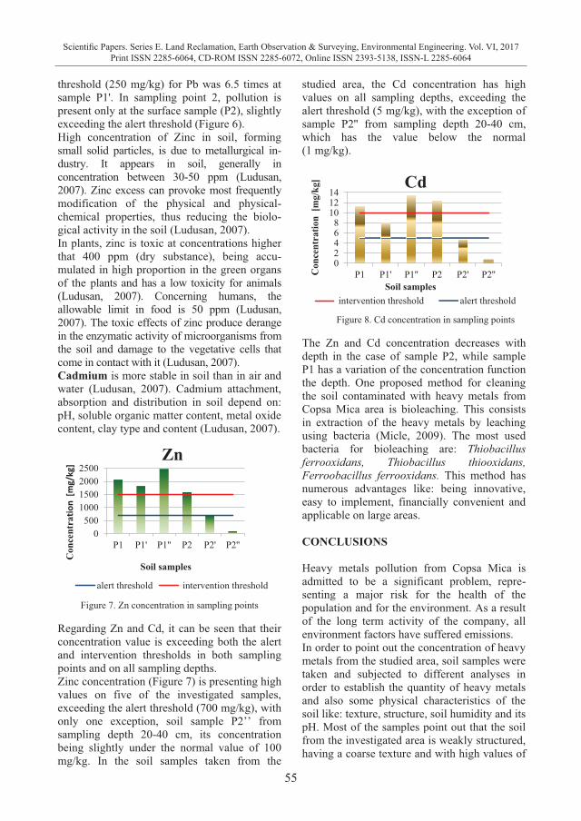
55
Scientific Papers. Series E. Land Reclamation, Earth Observation & Surveying, Environmental Engineering. Vol. VI, 2017Print ISSN 2285-6064, CD-ROM ISSN 2285-6072, Online ISSN 2393-5138, ISSN-L 2285-6064
threshold (250 mg/kg) for Pb was 6.5 times at sample P1'. In sampling point 2, pollution is present only at the surface sample (P2), slightly exceeding the alert threshold (Figure 6). High concentration of Zinc in soil, forming small solid particles, is due to metallurgical in-dustry. It appears in soil, generally in concentration between 30-50 ppm (Ludusan, 2007). Zinc excess can provoke most frequently modification of the physical and physical-chemical properties, thus reducing the biolo-gical activity in the soil (Ludusan, 2007). In plants, zinc is toxic at concentrations higher that 400 ppm (dry substance), being accu-mulated in high proportion in the green organs of the plants and has a low toxicity for animals (Ludusan, 2007). Concerning humans, the allowable limit in food is 50 ppm (Ludusan, 2007). The toxic effects of zinc produce derange in the enzymatic activity of microorganisms from the soil and damage to the vegetative cells that come in contact with it (Ludusan, 2007). Cadmium is more stable in soil than in air and water (Ludusan, 2007). Cadmium attachment, absorption and distribution in soil depend on: pH, soluble organic matter content, metal oxide content, clay type and content (Ludusan, 2007).
Figure 7. Zn concentration in sampling points
Regarding Zn and Cd, it can be seen that their concentration value is exceeding both the alert and intervention thresholds in both sampling points and on all sampling depths. Zinc concentration (Figure 7) is presenting high values on five of the investigated samples, exceeding the alert threshold (700 mg/kg), with only one exception, soil sample P2’’ from sampling depth 20-40 cm, its concentration being slightly under the normal value of 100 mg/kg. In the soil samples taken from the
studied area, the Cd concentration has high values on all sampling depths, exceeding the alert threshold (5 mg/kg), with the exception of sample P2'' from sampling depth 20-40 cm, which has the value below the normal (1 mg/kg).
Figure 8. Cd concentration in sampling points
The Zn and Cd concentration decreases with depth in the case of sample P2, while sample P1 has a variation of the concentration function the depth. One proposed method for cleaning the soil contaminated with heavy metals from Copsa Mica area is bioleaching. This consists in extraction of the heavy metals by leaching using bacteria (Micle, 2009). The most used bacteria for bioleaching are: Thiobacillus ferrooxidans, Thiobacillus thiooxidans, Ferroobacillus ferrooxidans. This method has numerous advantages like: being innovative, easy to implement, financially convenient and applicable on large areas. CONCLUSIONS Heavy metals pollution from Copsa Mica is admitted to be a significant problem, repre-senting a major risk for the health of the population and for the environment. As a result of the long term activity of the company, all environment factors have suffered emissions. In order to point out the concentration of heavy metals from the studied area, soil samples were taken and subjected to different analyses in order to establish the quantity of heavy metals and also some physical characteristics of the soil like: texture, structure, soil humidity and its pH. Most of the samples point out that the soil from the investigated area is weakly structured, having a coarse texture and with high values of
0500
1000150020002500
P1 P1' P1'' P2 P2' P2''
Zn
alert threshold intervention threshold
Con
cent
ratio
n [m
g/kg
]
Soil samples
02468
101214
P1 P1' P1'' P2 P2' P2''
Cd
intervention threshold alert thresholdC
once
ntra
tion
[mg/
kg]
Soil samples
56
Scientific Papers. Series E. Land Reclamation, Earth Observation & Surveying, Environmental Engineering. Vol. VI, 2017Print ISSN 2285-6064, CD-ROM ISSN 2285-6072, Online ISSN 2393-5138, ISSN-L 2285-6064
pH (>7). The Pb concentration in sampling point 1 exceeds the alert threshold and intervention threshold, and in sampling point 2, the pollution is present only at surface sample. The Zn and Cd concentration exceeds the alert and intervention threshold in both points in all three sampling depths. Zn and Cd concentration is decreasing with depth for sample P2, while sample P1 has a variation of the concentration function the depth. A proposed method for cleaning the soil from Copsa Mica area contaminated with heavy metals is bioleaching. This consists in extraction of the metals from the polluted soil by leaching, using bacteria (Micle, 2009). The most used bacteria for bioleaching are: Thiobacillus ferrooxidans, Thiobacillus thiooxidans, Ferroobacillus ferrooxidans. This method has numerous advantages like: being innovative, easy to implement, financially convenient and applicable on large areas. ACKNOWLEDGEMENTS This work was supported by a grant of the Romanian National Authority for Scientific Research, CNCS – UEFISCDI, project number PN II- PT-PCCA-2013-4-1717 (Project BIORESOL no. 91/2014). REFERENCES Berar (Sur) I. M., Micle V., Avram S., Senila M., Oros
V., 2012. Bioleaching of some heavy metals from polluted soils, Environmental Engineering and Management Journal, 11(8):1389-1393.
Botnariuc N., Vadineanu A., 1982. Ecology, Didactic and Pedagogical Publishing House, Bucharest (in Romanian).
Chen S.Y., Lin J.G., 2004. Bioleaching of heavy metals from contaminated sediment by indigenous sulfur-oxidizing bacteria in an air-lift bioreactor: Effects of sulfur concentration, Water Research 38(14-15):3205-3214.
Gadd G. M., 2004. Microbial influence on metal mobility and application for bioremediation, Geoderma, 122(2-4):109–119.
Groudev S.N., Georgiev P.S., Komnitsas K., 2001. In Situ Bioremediation of a Soil Contaminated with Heavy Metals and Arsenic, In: Leeson A., Peyton B.M., Means J.L., Magar V.S. (Eds.), Bioremediation of Inorganic Compounds: The Sixth International in Situ and On-Site Bioremediation Symposium, San Diego, California (June 4-7), 6:97-103.
Jayesh D.,Soumya D. M., Bioleaching of lateritic nickel ore using chemolithotrophic microorganisms (Acidithiobacillus ferrooxidans), National Institute of Technology Rourkela, 2007.
Liu Y.-G. , Ming Z., Guang-Ming Z., Xu W.-H , 2008. Bioleaching of heavy metals from mine tailings by indigenous sulfur-oxidizing bacteria: Effects of substrate concentration, Bioresource Technology, 99(10):4124-4129.
Ludusan N., 2007. Effects of heavy metals accumulation in soils on the biotic component in the Zlatna depression, Cadastre Magazine, 189-194 (in Romanian).
Micle V, Berar (Sur) Ioana Monica, 2012. Soil Science - Laboratory Guide, U.T. Press Publishing House, Cluj-Napoca (in Romanian).
Micle V., 2009. Ecological restoration of degraded areas, U.T. Press Publishing House, Cluj-Napoca (in Romanian).
Morarescu (Lupu) C., 2014. Model for assessing progress of intervention program in mitigating the risks associated with heavy metal exposure (Pb, Cd) in the Copsa Mica area, Phd thesis, Cluj-Napoca (in Romanian).
Satarupa R., Madhumita R., 2015. Bioleaching of Heavy Metals by Sulfur Oxidizing Bacteria: A Review International Research Journal of Environment Sciences 4(9):1-5.
Sucuturdean A., Micle V., 2011. The influence of the industrial dump S.C. Sometra S.A. Copsa Mica upon the quality of the river Visa, Metalurgia international, 26(1):65-68.
Sur I. M., Micle V., Gabor T., 2016. The influence of polluted soil aeration in the process of in situ bioleaching, Studia Universitatis Babes-Bolyai, Chemia, 61(3):355-364.
***2010, State of the Environment Report – North-west Region 6 - Chapter 4 Land Use (in Romanian).
Szanto (Prodan) M., Micle V., Gament E., Prodan V.C., 2012. Investigations on soil quality in the Copsa Mica area, Journal of Environmental Research and Protection, 31:110-116.
***STAS 7184/1-84. Soils. Sampling for soil and agrochemical studies (in Romanian).
***SR ISO 10381-6:1997. Soil quality. Part 6: Guidance on the collection, handling and storage of soil under aerobic conditions for the assessment of microbiological processes, biomass and diversity in the laboratory (in Romanian).
***SR ISO 11464:1998. The quality of soil. Pre-treatment of samples for physical-chemical analysis, (in Romanian).
***STAS 7184/9-79. Soils. Determination of humidity. (in Romanian).
***SR ISO 11465. Soil quality. Determination of dry matter and water content on a mass basis - gravimetric method (in Romanian).
***STAS 7184/13-88. Soils. Determination of pH (in Romanian).
***SR ISO 10390. Soil quality. Determination of pH. (in Romanian)..
57
Scientific Papers. Series E. Land Reclamation, Earth Observation & Surveying, Environmental Engineering. Vol. VI, 2017Print ISSN 2285-6064, CD-ROM ISSN 2285-6072, Online ISSN 2393-5138, ISSN-L 2285-6064
DETERMINATION OF THE AREAS SUITABLE FOR BIOGAS ENERGY
PRODUCTION BY USING GEOGRAPHIC INFORMATION SYSTEMS (GIS): EUPHRATES BASIN CASE
Burak SALTUK1, Ozan ARTUN2, Atilgan ATILGAN3
1Siirt University, 56100 Siirt, Turkey
2Cukurova University, 01770 Adana, Turkey 3Süleyman Demirel University, 32260 Isparta, Turkey
Corresponding author email: [email protected]
Abstract One of the agricultural activities in our country is animal breeding. The animal manure from cattle breeding enterprises can be used as an organic material in producing biogas. The energy needs of agricultural enterprises can be met by establishing biogas production facilities. At the same time, environmental pollution can also be prevented. With today's information and technology, it is possible to investigate the areas suitable for biogas energy stations. The aim of this study is to determine the potential areas in the Euphrates Basin which are suitable for biogas plants. The Euphrates Basin covers Adiyaman, Sanliurfa, Gaziantep and Kilis provinces. In this context, the borders of the provinces subjected to the study and the topographic properties of the region were drawn using ARCMAP 10.0 software. Furthermore, cattle numbers were entered into the Geographic Information Systems (GIS) database. The potential biogas areas in each province were determined and these areas were tried to be interpreted in different colours. In the study area, it was determined that the potential biogas energy of 862863.7 MJ or electricity energy of 239684.4 kWh would be obtained from approximately 2061883.4 tonnes of animal waste per year. It was determined that these values were equal to an amount of the annual energy capacity needs of 103 houses. Biogas energy production facilities can be established in the places which have an intensive agricultural activity and this can eliminate environmental pollution problems. Key words: biogas, GIS, Euphrates basin, cattle manure INTRODUCTION
Rapid population growth and industrialisation in developing countries cause a rapid increase in demand for energy (Onal and Yarbay, 2010; Koc and Senel, 2013). It is stated by researchers that a situation determination has to be made for energy resources in the world and in our country in order to ensure the planned use of energy resources facing the danger of exhaustion and to regulate the use of renewable energy resources (Koc and Senel, 2013). Due to both the decrease in costs and the necessity to increase the share of renewable energy worldwide, the use of these energy sources in energy production planning is recently required. Renewable energy sources are non-fossil energy sources such as hydropower, wind, sun, geothermal, biomass, biogas (including garbage gas), wave, discharge energy and tide (Ozcan et al., 2011).
The resulting gas mixture of the biodegradation of organic wastes in an anaerobic environment is called biogas. Especially in meeting rural energy needs, biogas, with the high production and abundance of raw materials and the high thermal value, can be considered as an energy source (Polat and Olgun, 2004). Biogas energy is a flammable gas resulting from the processing of biological materials. The difference of biogas from other flammable gases is that it is pro-duced only from vegetable and animal origin organic raw materials (Anonymous, 2006). Bioenergy is a biological, non-fossil organic matter. Biomass, which has sources such as agricultural and forestry products, vegetable wastes, marine plants, industrial and domestic wastes, is an environmentally friendly, renewable and local energy source that can respond to economic needs (Acaroglu, 2007; Ozturk, 2008). The wastes generated during the processing of vegetable products may be shown
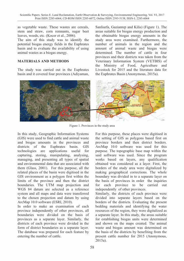
58
Scientific Papers. Series E. Land Reclamation, Earth Observation & Surveying, Environmental Engineering. Vol. VI, 2017Print ISSN 2285-6064, CD-ROM ISSN 2285-6072, Online ISSN 2393-5138, ISSN-L 2285-6064
as vegetable waste. These wastes are cereals, stem and straw, corn remnants, sugar beet leaves, weeds, etc. (Kocer et al., 2006). The aim of this study was to identify the potential biogas energy fields in the Euphrates basin and to evaluate the availability of using animal wastes as a biogas energy. MATERIALS AND METHODS The study was carried out in the Euphrates basin and it covered four provinces (Adiyaman,
Sanliurfa, Gaziantep and Kilis) (Figure 1). The areas suitable for biogas energy production and the obtainable biogas energy amounts in the study area were examined. Furthermore, the number of animals in the region and the amount of animal waste and biogas were determined. The number of cattle in four provinces and their districts was taken from the Veterinary Information System (VETBIS) of the Ministry of Food, Agriculture and Livestock for 2015 and the literature data for the Euphrates Basin (Anonymous, 2015a).
Figure 1. Provinces in the study area
In this study, Geographic Information Systems (GIS) were used to find cattle and animal waste and biogas amounts in the provinces and districts of the Euphrates basin. GIS technologies are applications useful for capturing, storing, manipulating, analysing, managing, and presenting all types of spatial and environmental data that are associated with them (Glass, 2001). For this purpose, all the related places of the basin were digitised in the GIS environment as a polygon first within the limits of the province and then the district boundaries. The UTM map projection and WGS 84 datum are selected as a reference system and all maps and data were transferred to the chosen projection and datum by using ArcMap 10.0 software (ESRI, 2010). In order to make an examination of each province independently of other provinces, all boundaries were divided on the basis of provinces as a separate layer. Similarly, the districts of each province were divided in the form of district boundaries as a separate layer. The database was prepared for each feature by entering the number of cattle.
For this purpose, these places were digitised in the setting of GIS as polygons based first on province borders and then district borders. ArcMap 10.0 software was used for this purpose. The topographic base map within the said software was used. Since the program works based on layers, any qualification obtained was considered as a layer. First, the borders of the study area were digitalized by making geographical corrections. The whole boundary was divided in to a separate layer on the basis of provinces in order the inquiries for each province to be carried out independently of other provinces. Similarly, the districts of each province were divided into separate layers based on the borders of the districts. Evaluating the present bedding materials and identifying the water resources of the region, they were digitalized as a separate layer. In this study, the areas suitable for establishing biogas units were determined and shown on the maps created. The animal waste and biogas amount was determined on the basis of the districts by benefiting from the present cattle number for 2015 (Anonymous, 2015a).
59
Scientific Papers. Series E. Land Reclamation, Earth Observation & Surveying, Environmental Engineering. Vol. VI, 2017Print ISSN 2285-6064, CD-ROM ISSN 2285-6072, Online ISSN 2393-5138, ISSN-L 2285-6064
as vegetable waste. These wastes are cereals, stem and straw, corn remnants, sugar beet leaves, weeds, etc. (Kocer et al., 2006). The aim of this study was to identify the potential biogas energy fields in the Euphrates basin and to evaluate the availability of using animal wastes as a biogas energy. MATERIALS AND METHODS The study was carried out in the Euphrates basin and it covered four provinces (Adiyaman,
Sanliurfa, Gaziantep and Kilis) (Figure 1). The areas suitable for biogas energy production and the obtainable biogas energy amounts in the study area were examined. Furthermore, the number of animals in the region and the amount of animal waste and biogas were determined. The number of cattle in four provinces and their districts was taken from the Veterinary Information System (VETBIS) of the Ministry of Food, Agriculture and Livestock for 2015 and the literature data for the Euphrates Basin (Anonymous, 2015a).
Figure 1. Provinces in the study area
In this study, Geographic Information Systems (GIS) were used to find cattle and animal waste and biogas amounts in the provinces and districts of the Euphrates basin. GIS technologies are applications useful for capturing, storing, manipulating, analysing, managing, and presenting all types of spatial and environmental data that are associated with them (Glass, 2001). For this purpose, all the related places of the basin were digitised in the GIS environment as a polygon first within the limits of the province and then the district boundaries. The UTM map projection and WGS 84 datum are selected as a reference system and all maps and data were transferred to the chosen projection and datum by using ArcMap 10.0 software (ESRI, 2010). In order to make an examination of each province independently of other provinces, all boundaries were divided on the basis of provinces as a separate layer. Similarly, the districts of each province were divided in the form of district boundaries as a separate layer. The database was prepared for each feature by entering the number of cattle.
For this purpose, these places were digitised in the setting of GIS as polygons based first on province borders and then district borders. ArcMap 10.0 software was used for this purpose. The topographic base map within the said software was used. Since the program works based on layers, any qualification obtained was considered as a layer. First, the borders of the study area were digitalized by making geographical corrections. The whole boundary was divided in to a separate layer on the basis of provinces in order the inquiries for each province to be carried out independently of other provinces. Similarly, the districts of each province were divided into separate layers based on the borders of the districts. Evaluating the present bedding materials and identifying the water resources of the region, they were digitalized as a separate layer. In this study, the areas suitable for establishing biogas units were determined and shown on the maps created. The animal waste and biogas amount was determined on the basis of the districts by benefiting from the present cattle number for 2015 (Anonymous, 2015a).
According to Hill (1982) and Ekinci et al. (2010), it is very important to determine the capacity before projecting biogas facilities. The calculation of biogas production quantities was performed taking into account the use of whole manure produced in the study area. For the calculation of the amount of manure, an average amount of 43 kg·day-1 of manure obtained from mature cattle can be taken as a basis. While producing the prediction map of the study area, the districts with cattle between 0 and 1000 heads were determined to be the areas not potential for biogas and colored in orange ( ), and the districts with cattle between 1000 and 10000 heads were determined to be potential biogas production areas and colored in yellow ( ). Again, the districts with more than 10000 heads of cattle were determined to be high-potential biogas production areas and coloured in green ( ). The prediction map of the suitable biogas production areas of the study area was created in relation to these animal numbers. The number of cattle in 2015 was evaluated within 3 layers and shown on the map of the basin by different colouring (Table 1). Table 1. Representation of the cattle number on the study
area map
Cattle Number in Enterprises
Display Colour on the Map
1-1.000 1.000-10.000 10.000-10.000+
RESULTS AND DISCUSSION When the provinces in the study area were compared with each other, it was seen that Gaziantep and Sanliurfa provinces take an important place both in terms of land area and animal numbers. In the study area, the total number of cattle was determined to be 57521 in Gaziantep province, 53795 in Sanliurfa province, 17078 in Adiyaman province and 2978 in for 2015 (Figure 2.). Upon examining the study area, it was determined that livestock breeding was performed at a lower level in Kilis province. In the study area, it was determined that the number of cattle increased due to population density, but that the number
of biogas-producing did not increase at the same rate. The Pilot Implementation of Increasing Energy Efficiency in the Industry, which is carried out in the region between 2014 and 2018, is aimed to increase the investment of the facilities in the study area with the financial support programs. It is believed that economic reasons and the difficulty of obtaining a qualified labour force in the region are the reasons for not increasing the investment in the animal husbandry and energy-producing industrial enterprises. Especially in the province of Gaziantep, where industrial investments have a large share, it can be stated that investors tend to orient to textile and machinery producing industrial establishments and put animal husbandry on the second plan.Other reasons for this are the facts that the number of the villages and the number of cattle in these villages are very low as a result of low population and hard topographic conditions in the province. In contrast, it was also determined that livestock breeding was performed at a significant level in Gaziantep and Sanliurfa provinces. These two provinces are followed by Adiyaman province. There are various ways to calculate the amount of wet manure and obtainable biogas energy in the literature. In the study area, the amount of wet manure and obtainable biogas energy were calculated according to Hill (1982) and Ekinci et al. (2010) using the number of animals in the study area, and the results are given in Table 2. In the calculation made according to Hill (1982) and Ekinci et al. (2010), it was determined that the highest amount of wet manure and obtainable biogas energy was in Gaziantep province. Gaziantep province was followed by Sanliurfa, Adiyaman and Kilis provinces, respectively. The calculation method of Hill (1982) and Ekinci et al. (2010) was also used separately for the districts of all provinces in the basin, and the amounts of wet, manure and potential biogas energy of these districts were calculated. Owing to these calculations, the appropriate places where biogas energy production facilities could be established in the provinces of the basin were tried.
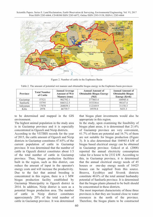
60
Scientific Papers. Series E. Land Reclamation, Earth Observation & Surveying, Environmental Engineering. Vol. VI, 2017Print ISSN 2285-6064, CD-ROM ISSN 2285-6072, Online ISSN 2393-5138, ISSN-L 2285-6064
Figure 2. Number of cattle in the Euphrates Basin
Table 2. The amount of potential wet manure and obtainable biogas energy in the Euphrates basin provinces
Province Total Number of Cattle
Annual Average Amount of Wet Manure (tons)
Annual Amount of Obtainable Biogas Energy
(MJ)
Annual Amount of Obtainable Biogas
Energy (Kwh) Gaziantep 57521 902792.1 377803.4 104945.4 Sanliurfa 53795 844312.5 353330.6 98147.4 Adiyaman 17078 268039.1 112169.9 31158.3
Kilis 2978 46739.7 19559.8 5433.3 to be determined and mapped in the GIS environment. The highest animal population in the study area is in Gaziantep province and it is especially concentrated in Oguzeli and Nizip districts. According to the VETBIS records for the year of 2015, the cattle amount of Oguzeli and Nizip districts in Gaziantep constitutes 47.65% of the current population of cattle in Gaziantep province. It was determined that the number of cattle in Oguzeli district constitutes about 1/3 of the total number of cattle in Gaziantep province. Thus, biogas production facilities built in the region, such as this district, can reduce the amount of input in the operator's energy costs and will increase the productivity. Due to the fact that animal breeding is concentrated in this region, there is a 1 MW biogas production facility established by Gaziantep Municipality in Oguzeli district in 2014. In addition, Nizip district is seen as a potential biogas production area. The number of cattle in Nizip district constitutes approximately 20% of the total number of cattle in Gaziantep province. It was determined
that biogas plant investments would also be appropriate in this region. In the study, upon examining the feasibility of biogas plant areas, it is determined that 21.6% of Gaziantep province are very convenient, 61.7% of them are potential and 16.7% of them are not suitable for biogas production (Figure 3). It is also determined that 104945.4 kW of biogas based electrical energy can be obtained in Gaziantep province. Gokcol et al. (2008) reported the annual electricity consumption value for a house to be 2332 kW. According to this, in Gaziantep province, it is determined that the annual electrical energy needs of 45 houses or one-day energy needs of 16425 houses can be supplied from this source. Bozova, Eyyübiye and Siverek districts constitute 40.6% of the total animal husbandry potential of Sanliurfa province. It is determined that the biogas plants planned to be built should be concentrated in these districts. The most important characteristic of these three provinces is that they are located close to water resources in the north of the province. Therefore, the biogas plants to be constructed
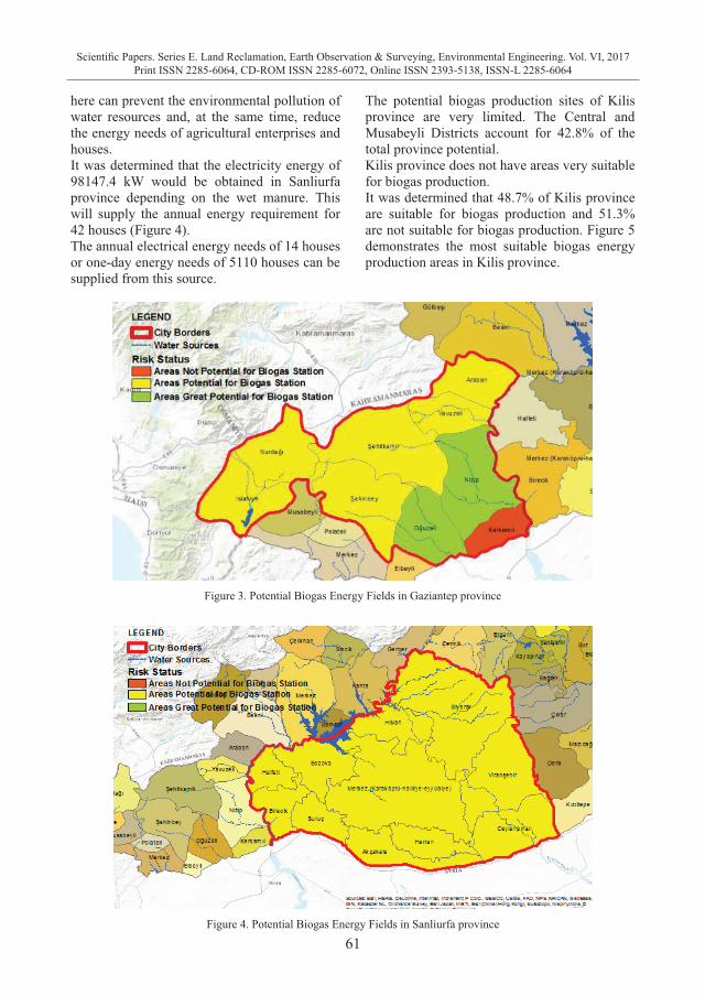
61
Scientific Papers. Series E. Land Reclamation, Earth Observation & Surveying, Environmental Engineering. Vol. VI, 2017Print ISSN 2285-6064, CD-ROM ISSN 2285-6072, Online ISSN 2393-5138, ISSN-L 2285-6064
Figure 2. Number of cattle in the Euphrates Basin
Table 2. The amount of potential wet manure and obtainable biogas energy in the Euphrates basin provinces
Province Total Number of Cattle
Annual Average Amount of Wet Manure (tons)
Annual Amount of Obtainable Biogas Energy
(MJ)
Annual Amount of Obtainable Biogas
Energy (Kwh) Gaziantep 57521 902792.1 377803.4 104945.4 Sanliurfa 53795 844312.5 353330.6 98147.4 Adiyaman 17078 268039.1 112169.9 31158.3
Kilis 2978 46739.7 19559.8 5433.3 to be determined and mapped in the GIS environment. The highest animal population in the study area is in Gaziantep province and it is especially concentrated in Oguzeli and Nizip districts. According to the VETBIS records for the year of 2015, the cattle amount of Oguzeli and Nizip districts in Gaziantep constitutes 47.65% of the current population of cattle in Gaziantep province. It was determined that the number of cattle in Oguzeli district constitutes about 1/3 of the total number of cattle in Gaziantep province. Thus, biogas production facilities built in the region, such as this district, can reduce the amount of input in the operator's energy costs and will increase the productivity. Due to the fact that animal breeding is concentrated in this region, there is a 1 MW biogas production facility established by Gaziantep Municipality in Oguzeli district in 2014. In addition, Nizip district is seen as a potential biogas production area. The number of cattle in Nizip district constitutes approximately 20% of the total number of cattle in Gaziantep province. It was determined
that biogas plant investments would also be appropriate in this region. In the study, upon examining the feasibility of biogas plant areas, it is determined that 21.6% of Gaziantep province are very convenient, 61.7% of them are potential and 16.7% of them are not suitable for biogas production (Figure 3). It is also determined that 104945.4 kW of biogas based electrical energy can be obtained in Gaziantep province. Gokcol et al. (2008) reported the annual electricity consumption value for a house to be 2332 kW. According to this, in Gaziantep province, it is determined that the annual electrical energy needs of 45 houses or one-day energy needs of 16425 houses can be supplied from this source. Bozova, Eyyübiye and Siverek districts constitute 40.6% of the total animal husbandry potential of Sanliurfa province. It is determined that the biogas plants planned to be built should be concentrated in these districts. The most important characteristic of these three provinces is that they are located close to water resources in the north of the province. Therefore, the biogas plants to be constructed
here can prevent the environmental pollution of water resources and, at the same time, reduce the energy needs of agricultural enterprises and houses. It was determined that the electricity energy of 98147.4 kW would be obtained in Sanliurfa province depending on the wet manure. This will supply the annual energy requirement for 42 houses (Figure 4). The annual electrical energy needs of 14 houses or one-day energy needs of 5110 houses can be supplied from this source.
The potential biogas production sites of Kilis province are very limited. The Central and Musabeyli Districts account for 42.8% of the total province potential. Kilis province does not have areas very suitable for biogas production. It was determined that 48.7% of Kilis province are suitable for biogas production and 51.3% are not suitable for biogas production. Figure 5 demonstrates the most suitable biogas energy production areas in Kilis province.
Figure 3. Potential Biogas Energy Fields in Gaziantep province
Figure 4. Potential Biogas Energy Fields in Sanliurfa province
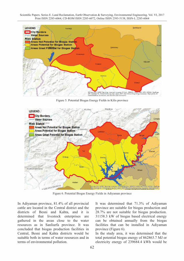
62
Scientific Papers. Series E. Land Reclamation, Earth Observation & Surveying, Environmental Engineering. Vol. VI, 2017Print ISSN 2285-6064, CD-ROM ISSN 2285-6072, Online ISSN 2393-5138, ISSN-L 2285-6064
Figure 5. Potential Biogas Energy Fields in Kilis province
Figure 6. Potential Biogas Energy Fields in Adiyaman province
In Adiyaman province, 81.4% of all provincial cattle are located in the Central district and the districts of Besni and Kahta, and it is determined that livestock enterprises are gathered in the areas close to the water resources as in Sanliurfa province. It was concluded that biogas production facilities in Central, Besni and Kahta districts would be suitable both in terms of water resources and in terms of environmental pollution.
It was determined that 71.3% of Adiyaman province are suitable for biogas production and 28.7% are not suitable for biogas production. 31158.3 kW of biogas based electrical energy can be obtained annually from the biogas facilities that can be installed in Adiyaman province (Figure 6). In the study area, it was determined that the total potential biogas energy of 862863.7 MJ or electricity energy of 239684.4 kWh would be
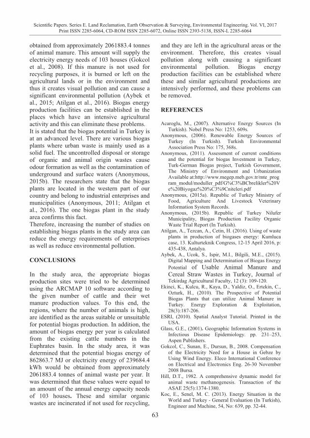
63
Scientific Papers. Series E. Land Reclamation, Earth Observation & Surveying, Environmental Engineering. Vol. VI, 2017Print ISSN 2285-6064, CD-ROM ISSN 2285-6072, Online ISSN 2393-5138, ISSN-L 2285-6064
Figure 5. Potential Biogas Energy Fields in Kilis province
Figure 6. Potential Biogas Energy Fields in Adiyaman province
In Adiyaman province, 81.4% of all provincial cattle are located in the Central district and the districts of Besni and Kahta, and it is determined that livestock enterprises are gathered in the areas close to the water resources as in Sanliurfa province. It was concluded that biogas production facilities in Central, Besni and Kahta districts would be suitable both in terms of water resources and in terms of environmental pollution.
It was determined that 71.3% of Adiyaman province are suitable for biogas production and 28.7% are not suitable for biogas production. 31158.3 kW of biogas based electrical energy can be obtained annually from the biogas facilities that can be installed in Adiyaman province (Figure 6). In the study area, it was determined that the total potential biogas energy of 862863.7 MJ or electricity energy of 239684.4 kWh would be
obtained from approximately 2061883.4 tonnes of animal manure. This amount will supply the electricity energy needs of 103 houses (Gokcol et al., 2008). If this manure is not used for recycling purposes, it is burned or left on the agricultural lands or in the environment and thus it creates visual pollution and can cause a significant environmental pollution (Aybek et al., 2015; Atilgan et al., 2016). Biogas energy production facilities can be established in the places which have an intensive agricultural activity and this can eliminate these problems. It is stated that the biogas potential in Turkey is at an advanced level. There are various biogas plants where urban waste is mainly used as a solid fuel. The uncontrolled disposal or storage of organic and animal origin wastes cause odour formation as well as the contamination of underground and surface waters (Anonymous, 2015b). The researchers state that the biogas plants are located in the western part of our country and belong to industrial enterprises and municipalities (Anonymous, 2011; Atilgan et al., 2016). The one biogas plant in the study area confirms this fact. Therefore, increasing the number of studies on establishing biogas plants in the study area can reduce the energy requirements of enterprises as well as reduce environmental pollution. CONCLUSIONS In the study area, the appropriate biogas production sites were tried to be determined using the ARCMAP 10 software according to the given number of cattle and their wet manure production values. To this end, the regions, where the number of animals is high, are identified as the areas suitable or unsuitable for potential biogas production. In addition, the amount of biogas energy per year is calculated from the existing cattle numbers in the Euphrates basin. In the study area, it was determined that the potential biogas energy of 862863.7 MJ or electricity energy of 239684.4 kWh would be obtained from approximately 2061883.4 tonnes of animal waste per year. It was determined that these values were equal to an amount of the annual energy capacity needs of 103 houses. These and similar organic wastes are incinerated if not used for recycling,
and they are left in the agricultural areas or the environment. Therefore, this creates visual pollution along with causing a significant environmental pollution. Biogas energy production facilities can be established where these and similar agricultural productions are intensively performed, and these problems can be removed. REFERENCES Acaroglu, M., (2007). Alternative Energy Sources (In
Turkish). Nobel Press No: 1253, 609s. Anonymous, (2006). Renewable Energy Sources of
Turkey (In Turkish). Turkish Environmental Association Press No: 175, 368s.
Anonymous, (2011). Assessment of current conditions and the potential for biogas Investment in Turkey, Turk-German Biogas project, Turkish Government, The Ministry of Environment and Urbanization Available at:http://www.megep.meb.gov.tr/mte_program_modul/moduller_pdf/G%C3%BCbrelikler%20Ve%20Biyogaz%20%C3%9Cniteleri.pdf
Anonymous, (2015a). Republic of Turkey Ministry of Food, Agriculture And Livestock Veterinary Information System Records.
Anonymous, (2015b). Republic of Turkey Nilufer Municipality, Biogas Production Facility Organic Waste Trial Report (In Turkish).
Atilgan, A., Tezcan, A., Cetin, H. (2016). Using of waste plants in production of biogases energy: Kumluca case, 13. Kulturteknik Congress, 12-15 April 2016, p: 435-438, Antalya.
Aybek, A., Ucok, S., Ispir, M.I., Bilgili, M.E., (2015). Digital Mapping and Determination of Biogas Energy Potential of Usable Animal Manure and Cereal Straw Wastes in Turkey, Journal of Tekirdag Agricultural Faculty, 12 (3): 109-120.
Ekinci, K., Kulcu, R., Kaya, D., Yaldiz, O., Ertekin, C., Ozturk, H., (2010). The Prospective of Potential Biogas Plants that can utilize Animal Manure in Turkey. Energy Exploration & Exploitation, 28(3):187-206.
ESRI, (2010). Spatial Analyst Tutorial. Printed in the USA.
Glass, G.E., (2001). Geographic Information Systems in Infectious Disease Epidemiology. pp. 231–253, Aspen Publishers.
Gokcol, C., Sunan, E., Dursun, B., 2008. Compensation of the Electricity Need for a House in Gebze by Using Wind Energy. Eleco International Conference on Electrical and Electronics Eng. 26-30 November 2008 Bursa.
Hill, D.T., 1982. A comprehensive dynamic model for animal waste methanogenesis. Transaction of the ASAE 25(5):1374-1380.
Koc, E., Senel, M. C. (2013). Energy Situation in the World and Turkey - General Evaluation (In Turkish), Engineer and Machine, 54, No: 639, pp. 32-44.

64
Scientific Papers. Series E. Land Reclamation, Earth Observation & Surveying, Environmental Engineering. Vol. VI, 2017Print ISSN 2285-6064, CD-ROM ISSN 2285-6072, Online ISSN 2393-5138, ISSN-L 2285-6064
Kocer, N.N. R., Oner, C., Sugozu, I., (2006). Livestock Production in Turkey and Biogas Potential (In Turkish). Eastern Anatolia Region Researches: 17–20.
Polat, H.E. and Olgun M. 2004. Design of Biogas Plants and Usage in Our Country (In Turkish) II. National Egean Energy Symposium, Dumlupınar University ,26-28 May 2004, p. 505-512, Kutahya.
Onal, E, Yarbay, R. Potential and Future of Renewable Energy Sources in Turkey (In Turkish) Istanbul
Trade University Journal of Science 9 (2010): 77-60.
Ozcan M., Ozturk S., Yıldırım M. (2011) Determination of Biogas Potentials of Turkey According to Different Source Types (In Turkish). Available at 23.01.2017 http://www.emo.org.tr/ekler/592515d4bc1ad62_ek.pdf
Ozturk, H. H., (2008). Renewable Energy Sources and their usage (In Turkish). Technic Press, 367p.
65
Scientific Papers. Series E. Land Reclamation, Earth Observation & Surveying, Environmental Engineering. Vol. VI, 2017Print ISSN 2285-6064, CD-ROM ISSN 2285-6072, Online ISSN 2393-5138, ISSN-L 2285-6064
Kocer, N.N. R., Oner, C., Sugozu, I., (2006). Livestock Production in Turkey and Biogas Potential (In Turkish). Eastern Anatolia Region Researches: 17–20.
Polat, H.E. and Olgun M. 2004. Design of Biogas Plants and Usage in Our Country (In Turkish) II. National Egean Energy Symposium, Dumlupınar University ,26-28 May 2004, p. 505-512, Kutahya.
Onal, E, Yarbay, R. Potential and Future of Renewable Energy Sources in Turkey (In Turkish) Istanbul
Trade University Journal of Science 9 (2010): 77-60.
Ozcan M., Ozturk S., Yıldırım M. (2011) Determination of Biogas Potentials of Turkey According to Different Source Types (In Turkish). Available at 23.01.2017 http://www.emo.org.tr/ekler/592515d4bc1ad62_ek.pdf
Ozturk, H. H., (2008). Renewable Energy Sources and their usage (In Turkish). Technic Press, 367p.
COMPARISON OF THE HEATING ENERGY REQUIREMENTS
OF THE GREENHOUSES IN THE TIGRIS BASIN WITH ANTALYA
Burak SALTUK1, Nazire MIKAIL1, Atilgan ATILGAN2, Yusuf AYDIN1
1Siirt University, 56100 Siirt, Turkey 2Suleyman Demirel University, 32260 Isparta, Turkey
Corresponding author email: [email protected]
Abstract The rapid growth of the world population also increases the amount of food needed for the human being's life. Therefore, applications that increase productivity and through which production can be made throughout the year in plant production come to the forefront in the world. In this context, one of the most important activities is greenhouse cultivation through which production can be made throughout the year by keeping climate conditions under control. Greenhouses are climate-controlled plant production structures in which indoor environment conditions can be controlled and can be kept in accordance with growing conditions. Heating must be performed during the winter period in greenhouses if it is desired to make production throughout the year. In Turkey, almost all of greenhouse production is performed in the Mediterranean region, and the production areas are situated in a relatively limited area in the Southeastern Anatolia Region. In this study, 10-year climate data (Maximum, Minimum and Average Temperature, Humidity, Sunshine Duration and Amounts) of 5 provinces (Diyarbakir, Mardin, Siirt, Batman and Sirnak) in the Tigris basin were achieved by considering the climatic conditions and production capacity of Antalya province, which has the most production areas in Turkey. According to the results obtained, the average minimum temperature for each month showed a statistically significant difference according to the provinces (p<0.01). Consequently, while the highest heating load was 1852.836 W/m2 for a greenhouse of 576 m2 for Antalya province in January during which heating requirement is the maximum, 3887.13 W/m2 and 5615 W/m2 heating load differences were obtained from Mardin and Diyarbakir provinces, respectively. Key words: Antalya, climate parameters, heating loads, temperature analysis of variance, Tigris basin. INTRODUCTION Applications in which climate conditions are kept under control and production can be made throughout the year are called greenhouse cultivation. Greenhouses are plant production structures realized in different forms for the purposes of producing various cultivated plants and their seeds, seedlings and saplings and protecting and displaying the plants by coating them with light transmissive materials such as glass, plastics, etc. and by keeping the factors such as temperature, light and humidity under control without being wholly or partially dependent on climate-related environmental conditions (Ones, 1986; Yaganoglu and Orung, 1997; Yuksel, 2000). The most extensive and effective environmentally controlled production takes place in greenhouses. New innovations and developments for greenhouse production go hand in hand with efforts for sustainability.
The greenhouses must be heated to ensure high yields and high quality. However, a high heating cost (20-60%) adversely influences production. The costs of the sustainability of greenhouse production can only be maintained with an increase in energy efficiency. The use of renewable energy sources in place of fossil fuels is theonly means to increase energy efficiency (Baytorun, 2016). Greenhouses provide a suitable environment for the intensive production of various crops. They are designed to control solar radiation, temperature, humidity and carbon dioxide levels in the aerial environment. The availability of solar radiation and its daily and yearly distribution have a tremendous influence on productivity and quality of plant growth and also on comfort living (Kania and Giacomelli, 2001). The most important energy requirement in the air-conditioning of greenhouses is realised in heating applications during the winter months. The expenses required for heating that is
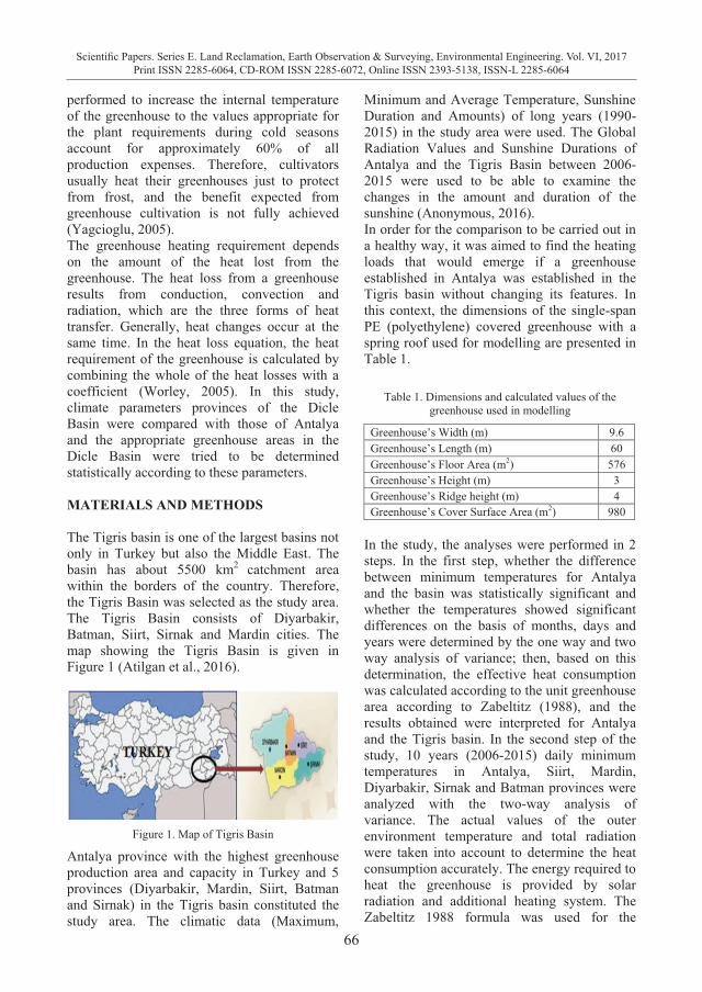
66
Scientific Papers. Series E. Land Reclamation, Earth Observation & Surveying, Environmental Engineering. Vol. VI, 2017Print ISSN 2285-6064, CD-ROM ISSN 2285-6072, Online ISSN 2393-5138, ISSN-L 2285-6064
performed to increase the internal temperature of the greenhouse to the values appropriate for the plant requirements during cold seasons account for approximately 60% of all production expenses. Therefore, cultivators usually heat their greenhouses just to protect from frost, and the benefit expected from greenhouse cultivation is not fully achieved (Yagcioglu, 2005). The greenhouse heating requirement depends on the amount of the heat lost from the greenhouse. The heat loss from a greenhouse results from conduction, convection and radiation, which are the three forms of heat transfer. Generally, heat changes occur at the same time. In the heat loss equation, the heat requirement of the greenhouse is calculated by combining the whole of the heat losses with a coefficient (Worley, 2005). In this study, climate parameters provinces of the Dicle Basin were compared with those of Antalya and the appropriate greenhouse areas in the Dicle Basin were tried to be determined statistically according to these parameters. MATERIALS AND METHODS The Tigris basin is one of the largest basins not only in Turkey but also the Middle East. The basin has about 5500 km2 catchment area within the borders of the country. Therefore, the Tigris Basin was selected as the study area. The Tigris Basin consists of Diyarbakir, Batman, Siirt, Sirnak and Mardin cities. The map showing the Tigris Basin is given in Figure 1 (Atilgan et al., 2016).
Figure 1. Map of Tigris Basin
Antalya province with the highest greenhouse production area and capacity in Turkey and 5 provinces (Diyarbakir, Mardin, Siirt, Batman and Sirnak) in the Tigris basin constituted the study area. The climatic data (Maximum,
Minimum and Average Temperature, Sunshine Duration and Amounts) of long years (1990-2015) in the study area were used. The Global Radiation Values and Sunshine Durations of Antalya and the Tigris Basin between 2006-2015 were used to be able to examine the changes in the amount and duration of the sunshine (Anonymous, 2016). In order for the comparison to be carried out in a healthy way, it was aimed to find the heating loads that would emerge if a greenhouse established in Antalya was established in the Tigris basin without changing its features. In this context, the dimensions of the single-span PE (polyethylene) covered greenhouse with a spring roof used for modelling are presented in Table 1.
Table 1. Dimensions and calculated values of the greenhouse used in modelling
Greenhouse’s Width (m) 9.6 Greenhouse’s Length (m) 60 Greenhouse’s Floor Area (m2) 576 Greenhouse’s Height (m) 3 Greenhouse’s Ridge height (m) 4 Greenhouse’s Cover Surface Area (m2) 980
In the study, the analyses were performed in 2 steps. In the first step, whether the difference between minimum temperatures for Antalya and the basin was statistically significant and whether the temperatures showed significant differences on the basis of months, days and years were determined by the one way and two way analysis of variance; then, based on this determination, the effective heat consumption was calculated according to the unit greenhouse area according to Zabeltitz (1988), and the results obtained were interpreted for Antalya and the Tigris basin. In the second step of the study, 10 years (2006-2015) daily minimum temperatures in Antalya, Siirt, Mardin, Diyarbakir, Sirnak and Batman provinces were analyzed with the two-way analysis of variance. The actual values of the outer environment temperature and total radiation were taken into account to determine the heat consumption accurately. The energy required to heat the greenhouse is provided by solar radiation and additional heating system. The Zabeltitz 1988 formula was used for the
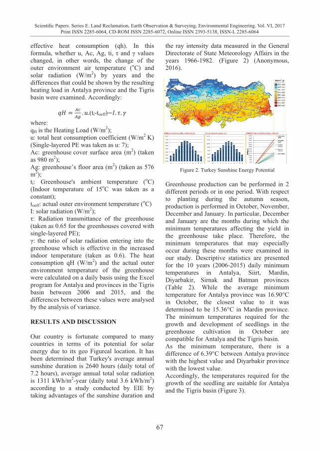
67
Scientific Papers. Series E. Land Reclamation, Earth Observation & Surveying, Environmental Engineering. Vol. VI, 2017Print ISSN 2285-6064, CD-ROM ISSN 2285-6072, Online ISSN 2393-5138, ISSN-L 2285-6064
performed to increase the internal temperature of the greenhouse to the values appropriate for the plant requirements during cold seasons account for approximately 60% of all production expenses. Therefore, cultivators usually heat their greenhouses just to protect from frost, and the benefit expected from greenhouse cultivation is not fully achieved (Yagcioglu, 2005). The greenhouse heating requirement depends on the amount of the heat lost from the greenhouse. The heat loss from a greenhouse results from conduction, convection and radiation, which are the three forms of heat transfer. Generally, heat changes occur at the same time. In the heat loss equation, the heat requirement of the greenhouse is calculated by combining the whole of the heat losses with a coefficient (Worley, 2005). In this study, climate parameters provinces of the Dicle Basin were compared with those of Antalya and the appropriate greenhouse areas in the Dicle Basin were tried to be determined statistically according to these parameters. MATERIALS AND METHODS The Tigris basin is one of the largest basins not only in Turkey but also the Middle East. The basin has about 5500 km2 catchment area within the borders of the country. Therefore, the Tigris Basin was selected as the study area. The Tigris Basin consists of Diyarbakir, Batman, Siirt, Sirnak and Mardin cities. The map showing the Tigris Basin is given in Figure 1 (Atilgan et al., 2016).
Figure 1. Map of Tigris Basin
Antalya province with the highest greenhouse production area and capacity in Turkey and 5 provinces (Diyarbakir, Mardin, Siirt, Batman and Sirnak) in the Tigris basin constituted the study area. The climatic data (Maximum,
Minimum and Average Temperature, Sunshine Duration and Amounts) of long years (1990-2015) in the study area were used. The Global Radiation Values and Sunshine Durations of Antalya and the Tigris Basin between 2006-2015 were used to be able to examine the changes in the amount and duration of the sunshine (Anonymous, 2016). In order for the comparison to be carried out in a healthy way, it was aimed to find the heating loads that would emerge if a greenhouse established in Antalya was established in the Tigris basin without changing its features. In this context, the dimensions of the single-span PE (polyethylene) covered greenhouse with a spring roof used for modelling are presented in Table 1.
Table 1. Dimensions and calculated values of the greenhouse used in modelling
Greenhouse’s Width (m) 9.6 Greenhouse’s Length (m) 60 Greenhouse’s Floor Area (m2) 576 Greenhouse’s Height (m) 3 Greenhouse’s Ridge height (m) 4 Greenhouse’s Cover Surface Area (m2) 980
In the study, the analyses were performed in 2 steps. In the first step, whether the difference between minimum temperatures for Antalya and the basin was statistically significant and whether the temperatures showed significant differences on the basis of months, days and years were determined by the one way and two way analysis of variance; then, based on this determination, the effective heat consumption was calculated according to the unit greenhouse area according to Zabeltitz (1988), and the results obtained were interpreted for Antalya and the Tigris basin. In the second step of the study, 10 years (2006-2015) daily minimum temperatures in Antalya, Siirt, Mardin, Diyarbakir, Sirnak and Batman provinces were analyzed with the two-way analysis of variance. The actual values of the outer environment temperature and total radiation were taken into account to determine the heat consumption accurately. The energy required to heat the greenhouse is provided by solar radiation and additional heating system. The Zabeltitz 1988 formula was used for the
effective heat consumption (qh). In this formula, whether u, Ac, Ag, ti, τ and γ values changed, in other words, the change of the outer environment air temperature (oC) and solar radiation (W/m2) by years and the differences that could be shown by the resulting heating load in Antalya province and the Tigris basin were examined. Accordingly:
(ti-toeff) where: qH is the Heating Load (W/m2); u: total heat consumption coefficient (W/m2 K) (Single-layered PE was taken as u: 7); Ac: greenhouse cover surface area (m2) (taken as 980 m2); Ag: greenhouse’s floor area (m2) (taken as 576 m2); ti: Greenhouse's ambient temperature (oC) (Indoor temperature of 15oC was taken as a constant); toeff: actual outer environment temperature (oC) I: solar radiation (W/m2); τ: Radiation transmittance of the greenhouse (taken as 0.65 for the greenhouses covered with single-layered PE); γ: the ratio of solar radiation entering into the greenhouse which is effective in the increased indoor temperature (taken as 0.6). The heat consumption qH (W/m2) and the actual outer environment temperature of the greenhouse were calculated on a daily basis using the Excel program for Antalya and provinces in the Tigris basin between 2006 and 2015, and the differences between these values were analysed by the analysis of variance. RESULTS AND DISCUSSION Our country is fortunate compared to many countries in terms of its potential for solar energy due to its geo Figureal location. It has been determined that Turkey's average annual sunshine duration is 2640 hours (daily total of 7.2 hours), average annual total solar radiation is 1311 kWh/m2-year (daily total 3.6 kWh/m2) according to a study conducted by EIE by taking advantages of the sunshine duration and
the ray intensity data measured in the General Directorate of State Meteorology Affairs in the years 1966-1982. (Figure 2) (Anonymous, 2016).
Figure 2. Turkey Sunshine Energy Potential
Greenhouse production can be performed in 2 different periods or in one period. With respect to planting during the autumn season, production is performed in October, November, December and January. In particular, December and January are the months during which the minimum temperatures affecting the yield in the greenhouse take place. Therefore, the minimum temperatures that may especially occur during these months were examined in our study. Descriptive statistics are presented for the 10 years (2006-2015) daily minimum temperatures in Antalya, Siirt, Mardin, Diyarbakir, Sirnak and Batman provinces (Table 2). While the average minimum temperature for Antalya province was 16.90°C in October, the closest value to it was determined to be 15.36°C in Mardin province. The minimum temperatures required for the growth and development of seedlings in the greenhouse cultivation in October are compatible for Antalya and the Tigris basin. As the minimum temperature, there is a difference of 6.39°C between Antalya province with the highest value and Diyarbakir province with the lowest value. Accordingly, the temperatures required for the growth of the seedling are suitable for Antalya and the Tigris basin (Figure 3).
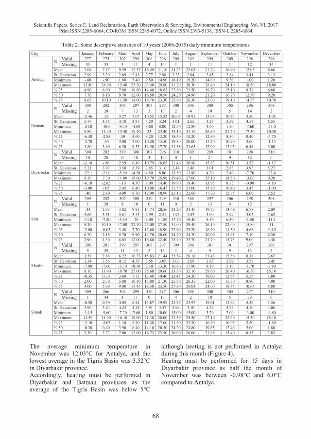
68
Scientific Papers. Series E. Land Reclamation, Earth Observation & Surveying, Environmental Engineering. Vol. VI, 2017Print ISSN 2285-6064, CD-ROM ISSN 2285-6072, Online ISSN 2393-5138, ISSN-L 2285-6064
Table 2. Some descriptive statistics of 10 years (2006-2015) daily minimum temperatures City January February Mart April May June July August September October November December
Antalya
N Valid 277 275 307 299 306 296 309 309 299 309 298 296 Missing 33 35 3 11 4 14 1 1 11 1 12 14
Mean 7.09 7.87 9.59 12.57 16.49 21.10 24.23 25.03 21.24 16.90 12.03 8.66 St. Deviation 2.99 3.29 2.69 2.43 2.77 2.98 2.23 2.04 2.45 2.84 3.41 3.13 Minimum -.60 -.90 1.80 5.40 9.50 14.90 18.10 19.20 14.60 9.30 1.00 1.20 Maximum 13.40 28.00 15.40 23.20 23.40 29.80 31.20 30.30 28.40 24.10 18.50 18.00 % 25 4.90 6.00 7.80 10.90 14.40 18.83 22.80 23.50 19.70 15.10 9.78 6.60 % 50 7.70 8.10 9.70 12.60 16.50 20.50 24.20 24.90 21.20 16.70 12.30 9.20 % 75 9.65 10.10 11.50 14.00 18.70 23.30 25.80 26.30 23.00 19.10 14.53 10.70
Batman
N Valid 308 282 303 297 307 297 308 306 300 305 296 308 Missing 2 28 7 13 3 13 2 4 10 5 14 2
Mean -2.46 .23 3.27 7.07 10.52 15.52 20.03 19.91 15.03 10.74 3.50 -1.05 St. Deviation 5.76 4.55 4.18 3.87 3.29 3.24 3.01 2.65 3.27 3.59 4.57 5.55 Minimum -24.0 -10.6 -8.50 -4.60 3.60 8.00 12.50 12.80 4.60 1.50 -7.60 -23.0 Maximum 8.80 11.40 15.40 19.20 23 25.40 33.10 31.10 26.80 21.20 17.50 10.30 % 25 -6.48 -2.85 .50 4.60 8.20 13.20 18.30 18.20 12.80 8.50 0.40 -4.70 % 50 -2.70 .60 3.00 7.00 10.20 15.50 19.80 20.00 15.20 10.90 3.00 -1.15 % 75 1.80 3.60 6.20 9.55 12.50 17.70 21.58 21.63 17.00 13.05 6.48 3.00
Diyarbakir
N Valid 300 282 310 300 307 296 310 309 289 301 298 310 Missing 10 28 0 10 3 14 0 1 21 9 12 0
Mean -3.10 -.56 2.59 6.49 10.79 16.65 21.46 20.96 15.83 10.51 3.52 -1.17 St. Deviation 5.21 3.97 3.50 3.39 2.85 3.16 2.44 2.46 3.01 2.83 3.95 5.27 Minimum -22.1 -21.0 -5.00 -4.20 4.50 8.80 13.50 13.80 4.20 2.40 -7.70 -23.4 Maximum 8.20 7.30 11.80 19.00 19.70 25.90 29.40 27.00 25.10 18.50 13.00 9.20 % 25 -6.18 -2.85 -.10 4.30 8.90 14.40 19.90 19.40 13.95 8.75 -0.98 -4.10 % 50 -3.00 -.05 2.45 6.40 10.80 16.45 21.50 21.00 15.80 10.40 3.45 -1.00 % 75 .40 2.40 4.90 8.70 12.90 18.90 23.10 22.60 17.80 12.35 6.00 2.52
Siirt
N Valid 309 282 302 300 310 299 310 308 297 306 298 308 Missing 1 28 8 10 0 11 0 2 13 4 12 2
Mean .34 2.03 5.82 9.95 14.74 20.56 24.20 24.46 19.75 13.69 6.78 2.09 St. Deviation 3.60 3.31 3.61 3.43 2.99 2.51 1.95 1.87 3.00 2.99 3.05 3.62 Minimum -11.0 -7.20 -3.60 .70 8.00 11.80 17.70 19.40 8.50 6.30 -1.50 -11.1 Maximum 9.20 10.10 17.00 22.40 25.00 27.50 31.00 29.40 26.10 22.00 15.80 11 % 25 -2.00 -0.03 3.48 7.70 12.60 18.90 22.90 23.20 18.20 11.50 4.68 -0.10 % 50 0.70 2.15 5.70 9.90 14.70 20.60 24.20 24.70 20.00 13.65 7.10 2.30 % 75 2.90 4.30 8.03 12.00 16.80 22.40 25.40 25.70 21.70 15.73 9.00 4.48
Mardin
N Valid 305 281 299 297 308 297 309 306 301 301 297 308 Missing 5 29 11 13 2 13 1 4 9 9 13 2
Mean 1.58 2.68 6.22 10.73 15.83 21.44 25.34 26.18 21.43 15.36 8.18 3.67 St. Deviation 3.34 3.56 4.12 4.39 3.65 3.05 3.06 2.69 3.83 3.89 3.57 3.45 Minimum -7.80 -7.60 -3.70 -0.10 7.30 13.30 16.60 17.90 8.10 5.10 -1.70 -7.80 Maximum 8.10 11.40 18.70 25.00 25.60 29.60 33.30 32.10 29.60 26.40 16.50 15.10 % 25 -0.35 0.70 3.60 7.75 13.40 19.40 23.45 24.20 19.00 12.95 5.55 1.80 % 50 2.00 2.70 5.80 10.30 15.80 21.30 25.60 26.35 22.00 15.50 8.80 4.00 % 75 4.00 5.00 9.00 13.45 18.30 23.50 27.30 28.03 24.00 18.35 10.65 5.80
Sirnak
N Valid 309 266 306 299 310 297 306 308 300 305 277 310 Missing 1 44 4 11 0 13 4 2 10 5 33 0
Mean -0.58 0.39 4.05 8.44 13.87 19.99 23.79 23.97 19.01 12.64 5.36 1.36 St. Deviation 3.96 3.94 4.23 4.52 3.91 3.37 2.99 3.10 4.22 3.75 4.10 4.06 Minimum -14.5 -9.60 -7.20 -2.60 1.80 10.00 15.00 15.00 3.20 2.00 -3.00 -9.80 Maximum 11.50 11.00 16.10 19.00 21.30 28.00 31.50 29.50 27.10 22.60 15.30 15.10 % 25 -3.10 -2.03 1.10 5.20 11.48 17.60 21.50 22.20 16.60 10.05 2.50 -1.80 % 50 -0.20 0.40 3.90 8.40 14.10 20.30 24.20 24.80 19.65 12.40 5.00 1.80 % 75 2.30 2.73 7.00 12.00 16.73 22.50 26.00 26.00 21.98 15.40 8.15 3.83
The average minimum temperature in November was 12.03°C for Antalya, and the lowest average in the Tigris Basin was 3.52°C in Diyarbakir province. Accordingly, heating must be performed in Diyarbakir and Batman provinces as the average of the Tigris Basin was below 5°C
although heating is not performed in Antalya during this month (Figure 4). Heating must be performed for 15 days in Diyarbakir province as half the month of November was between -0.98°C and 6.0°C compared to Antalya.
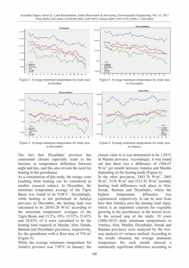
69
Scientific Papers. Series E. Land Reclamation, Earth Observation & Surveying, Environmental Engineering. Vol. VI, 2017Print ISSN 2285-6064, CD-ROM ISSN 2285-6072, Online ISSN 2393-5138, ISSN-L 2285-6064
Table 2. Some descriptive statistics of 10 years (2006-2015) daily minimum temperatures City January February Mart April May June July August September October November December
Antalya
N Valid 277 275 307 299 306 296 309 309 299 309 298 296 Missing 33 35 3 11 4 14 1 1 11 1 12 14
Mean 7.09 7.87 9.59 12.57 16.49 21.10 24.23 25.03 21.24 16.90 12.03 8.66 St. Deviation 2.99 3.29 2.69 2.43 2.77 2.98 2.23 2.04 2.45 2.84 3.41 3.13 Minimum -.60 -.90 1.80 5.40 9.50 14.90 18.10 19.20 14.60 9.30 1.00 1.20 Maximum 13.40 28.00 15.40 23.20 23.40 29.80 31.20 30.30 28.40 24.10 18.50 18.00 % 25 4.90 6.00 7.80 10.90 14.40 18.83 22.80 23.50 19.70 15.10 9.78 6.60 % 50 7.70 8.10 9.70 12.60 16.50 20.50 24.20 24.90 21.20 16.70 12.30 9.20 % 75 9.65 10.10 11.50 14.00 18.70 23.30 25.80 26.30 23.00 19.10 14.53 10.70
Batman
N Valid 308 282 303 297 307 297 308 306 300 305 296 308 Missing 2 28 7 13 3 13 2 4 10 5 14 2
Mean -2.46 .23 3.27 7.07 10.52 15.52 20.03 19.91 15.03 10.74 3.50 -1.05 St. Deviation 5.76 4.55 4.18 3.87 3.29 3.24 3.01 2.65 3.27 3.59 4.57 5.55 Minimum -24.0 -10.6 -8.50 -4.60 3.60 8.00 12.50 12.80 4.60 1.50 -7.60 -23.0 Maximum 8.80 11.40 15.40 19.20 23 25.40 33.10 31.10 26.80 21.20 17.50 10.30 % 25 -6.48 -2.85 .50 4.60 8.20 13.20 18.30 18.20 12.80 8.50 0.40 -4.70 % 50 -2.70 .60 3.00 7.00 10.20 15.50 19.80 20.00 15.20 10.90 3.00 -1.15 % 75 1.80 3.60 6.20 9.55 12.50 17.70 21.58 21.63 17.00 13.05 6.48 3.00
Diyarbakir
N Valid 300 282 310 300 307 296 310 309 289 301 298 310 Missing 10 28 0 10 3 14 0 1 21 9 12 0
Mean -3.10 -.56 2.59 6.49 10.79 16.65 21.46 20.96 15.83 10.51 3.52 -1.17 St. Deviation 5.21 3.97 3.50 3.39 2.85 3.16 2.44 2.46 3.01 2.83 3.95 5.27 Minimum -22.1 -21.0 -5.00 -4.20 4.50 8.80 13.50 13.80 4.20 2.40 -7.70 -23.4 Maximum 8.20 7.30 11.80 19.00 19.70 25.90 29.40 27.00 25.10 18.50 13.00 9.20 % 25 -6.18 -2.85 -.10 4.30 8.90 14.40 19.90 19.40 13.95 8.75 -0.98 -4.10 % 50 -3.00 -.05 2.45 6.40 10.80 16.45 21.50 21.00 15.80 10.40 3.45 -1.00 % 75 .40 2.40 4.90 8.70 12.90 18.90 23.10 22.60 17.80 12.35 6.00 2.52
Siirt
N Valid 309 282 302 300 310 299 310 308 297 306 298 308 Missing 1 28 8 10 0 11 0 2 13 4 12 2
Mean .34 2.03 5.82 9.95 14.74 20.56 24.20 24.46 19.75 13.69 6.78 2.09 St. Deviation 3.60 3.31 3.61 3.43 2.99 2.51 1.95 1.87 3.00 2.99 3.05 3.62 Minimum -11.0 -7.20 -3.60 .70 8.00 11.80 17.70 19.40 8.50 6.30 -1.50 -11.1 Maximum 9.20 10.10 17.00 22.40 25.00 27.50 31.00 29.40 26.10 22.00 15.80 11 % 25 -2.00 -0.03 3.48 7.70 12.60 18.90 22.90 23.20 18.20 11.50 4.68 -0.10 % 50 0.70 2.15 5.70 9.90 14.70 20.60 24.20 24.70 20.00 13.65 7.10 2.30 % 75 2.90 4.30 8.03 12.00 16.80 22.40 25.40 25.70 21.70 15.73 9.00 4.48
Mardin
N Valid 305 281 299 297 308 297 309 306 301 301 297 308 Missing 5 29 11 13 2 13 1 4 9 9 13 2
Mean 1.58 2.68 6.22 10.73 15.83 21.44 25.34 26.18 21.43 15.36 8.18 3.67 St. Deviation 3.34 3.56 4.12 4.39 3.65 3.05 3.06 2.69 3.83 3.89 3.57 3.45 Minimum -7.80 -7.60 -3.70 -0.10 7.30 13.30 16.60 17.90 8.10 5.10 -1.70 -7.80 Maximum 8.10 11.40 18.70 25.00 25.60 29.60 33.30 32.10 29.60 26.40 16.50 15.10 % 25 -0.35 0.70 3.60 7.75 13.40 19.40 23.45 24.20 19.00 12.95 5.55 1.80 % 50 2.00 2.70 5.80 10.30 15.80 21.30 25.60 26.35 22.00 15.50 8.80 4.00 % 75 4.00 5.00 9.00 13.45 18.30 23.50 27.30 28.03 24.00 18.35 10.65 5.80
Sirnak
N Valid 309 266 306 299 310 297 306 308 300 305 277 310 Missing 1 44 4 11 0 13 4 2 10 5 33 0
Mean -0.58 0.39 4.05 8.44 13.87 19.99 23.79 23.97 19.01 12.64 5.36 1.36 St. Deviation 3.96 3.94 4.23 4.52 3.91 3.37 2.99 3.10 4.22 3.75 4.10 4.06 Minimum -14.5 -9.60 -7.20 -2.60 1.80 10.00 15.00 15.00 3.20 2.00 -3.00 -9.80 Maximum 11.50 11.00 16.10 19.00 21.30 28.00 31.50 29.50 27.10 22.60 15.30 15.10 % 25 -3.10 -2.03 1.10 5.20 11.48 17.60 21.50 22.20 16.60 10.05 2.50 -1.80 % 50 -0.20 0.40 3.90 8.40 14.10 20.30 24.20 24.80 19.65 12.40 5.00 1.80 % 75 2.30 2.73 7.00 12.00 16.73 22.50 26.00 26.00 21.98 15.40 8.15 3.83
The average minimum temperature in November was 12.03°C for Antalya, and the lowest average in the Tigris Basin was 3.52°C in Diyarbakir province. Accordingly, heating must be performed in Diyarbakir and Batman provinces as the average of the Tigris Basin was below 5°C
although heating is not performed in Antalya during this month (Figure 4). Heating must be performed for 15 days in Diyarbakir province as half the month of November was between -0.98°C and 6.0°C compared to Antalya.
Figure 3. Average minimum temperature for study area
in October Figure 4. Average minimum temperature for study area
in November
Figure 5. Average minimum temperature for study area
in December Figure 6. Average minimum temperature for study area
in January
The fact that Diyarbakir province has continental climate especially leads to the increase in temperature difference between night and day, and this also reveals the need for heating in the greenhouse. As a continuation of this study, the energy costs resulting from heating can be considered as another research subject. In December, the minimum temperature average of the Tigris Basin was found to be 0.98°C. Accordingly, while heating is not performed in Antalya province in December, the heating load was calculated to be 20543.28 W/m2 according to the minimum temperature averages of the Tigris Basin, and 15.2%, 18%, 19.32%, 23.65% and 28.83% of it were calculated to be the heating load required in Mardin, Siirt, Sirnak, Batman and Diyarbakir provinces, respectively, for the greenhouse with a floor area of 576 m2
(Figure 5). While the average minimum temperature for Antalya province was 7.09°C in January, the
closest value to it was determined to be 1.58°C in Mardin province. Accordingly, it was found out that there was a difference of 1968.67 W/m2 per month between Antalya and Mardin depending on the heating loads (Figure 6). In the other provinces, 2463.70 W/m2, 2803 W/m2, 3126 W/m2 and 3221.82 W/m2 monthly heating load differences took place in Siirt, Sirnak, Batman and Diyarbakir, where the highest temperature difference was experienced, respectively. It can be seen from here that Antalya uses the heating load input, which is an important criterion for vegetable growing in the greenhouse, at the lowest level. In the second step of the study, 10 years (2006-2015) daily minimum temperatures in Antalya, Siirt, Mardin, Diyarbakir, Sirnak and Batman provinces were analysed by the two-way analysis of variance method. According to the results obtained, the average minimum temperature for each month showed a statistically significant difference according to
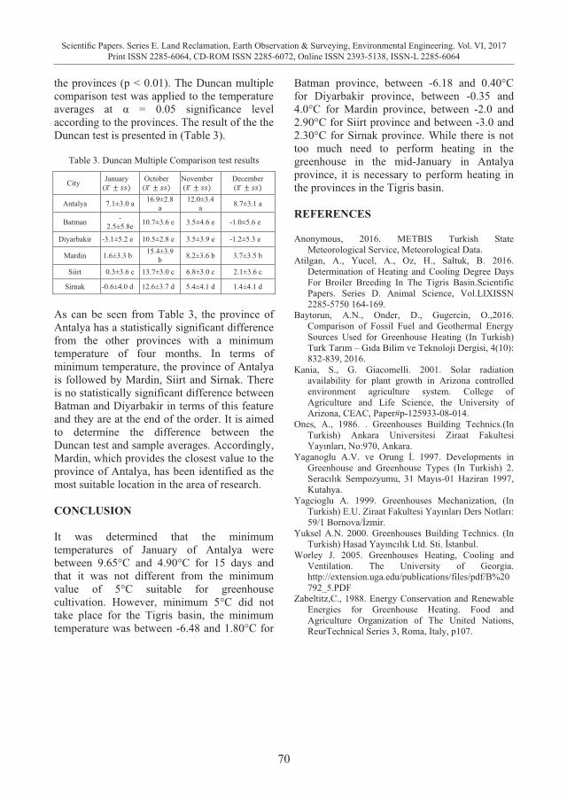
70
Scientific Papers. Series E. Land Reclamation, Earth Observation & Surveying, Environmental Engineering. Vol. VI, 2017Print ISSN 2285-6064, CD-ROM ISSN 2285-6072, Online ISSN 2393-5138, ISSN-L 2285-6064
the provinces (p < 0.01). The Duncan multiple comparison test was applied to the temperature averages at α = 0.05 significance level according to the provinces. The result of the the Duncan test is presented in (Table 3).
Table 3. Duncan Multiple Comparison test results
City January (
October (
November (
December (
Antalya 7.1±3.0 a 16.9±2.8 a
12.0±3.4 a 8.7±3.1 a
Batman -2.5±5.8e 10.7±3.6 e 3.5±4.6 e -1.0±5.6 e
Diyarbakir -3.1±5.2 e 10.5±2.8 e 3.5±3.9 e -1.2±5.3 e
Mardin 1.6±3.3 b 15.4±3.9b 8.2±3.6 b 3.7±3.5 b
Siirt 0.3±3.6 c 13.7±3.0 c 6.8±3.0 c 2.1±3.6 c
Sirnak -0.6±4.0 d 12.6±3.7 d 5.4±4.1 d 1.4±4.1 d
As can be seen from Table 3, the province of Antalya has a statistically significant difference from the other provinces with a minimum temperature of four months. In terms of minimum temperature, the province of Antalya is followed by Mardin, Siirt and Sirnak. There is no statistically significant difference between Batman and Diyarbakir in terms of this feature and they are at the end of the order. It is aimed to determine the difference between the Duncan test and sample averages. Accordingly, Mardin, which provides the closest value to the province of Antalya, has been identified as the most suitable location in the area of research. CONCLUSION It was determined that the minimum temperatures of January of Antalya were between 9.65°C and 4.90°C for 15 days and that it was not different from the minimum value of 5°C suitable for greenhouse cultivation. However, minimum 5°C did not take place for the Tigris basin, the minimum temperature was between -6.48 and 1.80°C for
Batman province, between -6.18 and 0.40°C for Diyarbakir province, between -0.35 and 4.0°C for Mardin province, between -2.0 and 2.90°C for Siirt province and between -3.0 and 2.30°C for Sirnak province. While there is not too much need to perform heating in the greenhouse in the mid-January in Antalya province, it is necessary to perform heating in the provinces in the Tigris basin. REFERENCES Anonymous, 2016. METBIS Turkish State
Meteorological Service, Meteorological Data. Atilgan, A., Yucel, A., Oz, H., Saltuk, B. 2016.
Determination of Heating and Cooling Degree Days For Broiler Breeding In The Tigris Basin.Scientific Papers. Series D. Animal Science, Vol.LIXISSN 2285-5750 164-169.
Baytorun, A.N., Onder, D., Gugercin, O.,2016. Comparison of Fossil Fuel and Geothermal Energy Sources Used for Greenhouse Heating (In Turkish) Turk Tarım – Gıda Bilim ve Teknoloji Dergisi, 4(10): 832-839, 2016.
Kania, S., G. Giacomelli. 2001. Solar radiation availability for plant growth in Arizona controlled environment agriculture system. College of Agriculture and Life Science, the University of Arizona, CEAC, Paper#p-125933-08-014.
Ones, A., 1986. . Greenhouses Building Technics.(In Turkish) Ankara Universitesi Ziraat Fakultesi Yayınları, No:970, Ankara.
Yaganoglu A.V. ve Orung İ. 1997. Developments in Greenhouse and Greenhouse Types (In Turkish) 2. Seracılık Sempozyumu, 31 Mayıs-01 Haziran 1997, Kutahya.
Yagcioglu A. 1999. Greenhouses Mechanization, (In Turkish) E.U. Ziraat Fakultesi Yayınları Ders Notları: 59/1 Bornova/İzmir.
Yuksel A.N. 2000. Greenhouses Building Technics. (In Turkish) Hasad Yayıncılık Ltd. Sti. İstanbul.
Worley J. 2005. Greenhouses Heating, Cooling and Ventilation. The University of Georgia. http://extension.uga.edu/publications/files/pdf/B%20792_5.PDF
Zabeltitz,C., 1988. Energy Conservation and Renewable Energies for Greenhouse Heating. Food and Agriculture Organization of The United Nations, ReurTechnical Series 3, Roma, Italy, p107.
71
Scientific Papers. Series E. Land Reclamation, Earth Observation & Surveying, Environmental Engineering. Vol. VI, 2017Print ISSN 2285-6064, CD-ROM ISSN 2285-6072, Online ISSN 2393-5138, ISSN-L 2285-6064
the provinces (p < 0.01). The Duncan multiple comparison test was applied to the temperature averages at α = 0.05 significance level according to the provinces. The result of the the Duncan test is presented in (Table 3).
Table 3. Duncan Multiple Comparison test results
City January (
October (
November (
December (
Antalya 7.1±3.0 a 16.9±2.8 a
12.0±3.4 a 8.7±3.1 a
Batman -2.5±5.8e 10.7±3.6 e 3.5±4.6 e -1.0±5.6 e
Diyarbakir -3.1±5.2 e 10.5±2.8 e 3.5±3.9 e -1.2±5.3 e
Mardin 1.6±3.3 b 15.4±3.9b 8.2±3.6 b 3.7±3.5 b
Siirt 0.3±3.6 c 13.7±3.0 c 6.8±3.0 c 2.1±3.6 c
Sirnak -0.6±4.0 d 12.6±3.7 d 5.4±4.1 d 1.4±4.1 d
As can be seen from Table 3, the province of Antalya has a statistically significant difference from the other provinces with a minimum temperature of four months. In terms of minimum temperature, the province of Antalya is followed by Mardin, Siirt and Sirnak. There is no statistically significant difference between Batman and Diyarbakir in terms of this feature and they are at the end of the order. It is aimed to determine the difference between the Duncan test and sample averages. Accordingly, Mardin, which provides the closest value to the province of Antalya, has been identified as the most suitable location in the area of research. CONCLUSION It was determined that the minimum temperatures of January of Antalya were between 9.65°C and 4.90°C for 15 days and that it was not different from the minimum value of 5°C suitable for greenhouse cultivation. However, minimum 5°C did not take place for the Tigris basin, the minimum temperature was between -6.48 and 1.80°C for
Batman province, between -6.18 and 0.40°C for Diyarbakir province, between -0.35 and 4.0°C for Mardin province, between -2.0 and 2.90°C for Siirt province and between -3.0 and 2.30°C for Sirnak province. While there is not too much need to perform heating in the greenhouse in the mid-January in Antalya province, it is necessary to perform heating in the provinces in the Tigris basin. REFERENCES Anonymous, 2016. METBIS Turkish State
Meteorological Service, Meteorological Data. Atilgan, A., Yucel, A., Oz, H., Saltuk, B. 2016.
Determination of Heating and Cooling Degree Days For Broiler Breeding In The Tigris Basin.Scientific Papers. Series D. Animal Science, Vol.LIXISSN 2285-5750 164-169.
Baytorun, A.N., Onder, D., Gugercin, O.,2016. Comparison of Fossil Fuel and Geothermal Energy Sources Used for Greenhouse Heating (In Turkish) Turk Tarım – Gıda Bilim ve Teknoloji Dergisi, 4(10): 832-839, 2016.
Kania, S., G. Giacomelli. 2001. Solar radiation availability for plant growth in Arizona controlled environment agriculture system. College of Agriculture and Life Science, the University of Arizona, CEAC, Paper#p-125933-08-014.
Ones, A., 1986. . Greenhouses Building Technics.(In Turkish) Ankara Universitesi Ziraat Fakultesi Yayınları, No:970, Ankara.
Yaganoglu A.V. ve Orung İ. 1997. Developments in Greenhouse and Greenhouse Types (In Turkish) 2. Seracılık Sempozyumu, 31 Mayıs-01 Haziran 1997, Kutahya.
Yagcioglu A. 1999. Greenhouses Mechanization, (In Turkish) E.U. Ziraat Fakultesi Yayınları Ders Notları: 59/1 Bornova/İzmir.
Yuksel A.N. 2000. Greenhouses Building Technics. (In Turkish) Hasad Yayıncılık Ltd. Sti. İstanbul.
Worley J. 2005. Greenhouses Heating, Cooling and Ventilation. The University of Georgia. http://extension.uga.edu/publications/files/pdf/B%20792_5.PDF
Zabeltitz,C., 1988. Energy Conservation and Renewable Energies for Greenhouse Heating. Food and Agriculture Organization of The United Nations, ReurTechnical Series 3, Roma, Italy, p107.
LAND RECLAMATION WORKS OPPORTUNITY
AND FEASIBILITY IN CLIMATE CHANGE CONTEXT
Dragos DRACEA, Augustina TRONAC, Sebastian MUSTATA
University of Agronomic Sciences and Veterinary Medicine of Bucharest, 59 Marasti Blvd, District 1, Bucharest, Romania
Corresponding author email: [email protected]
Abstract Land reclamation works are distributed across the territory, their positions being related to in situ factors. The governmental entity responsible off is the National Administration for Land Reclamation Works in Romania, administrating aprox. 3 million possible irrigated hectares, 3.1 million hectares possible drained, 2.2 million hectares equipped with soil erosion control works. Existing land reclamation systems shows different technical or/and economical deficiency taking in consideration the climatic changes evidenced by the evolution of temperatures, rainfall events distribution and intensity.. The comparison made with European countries goes to technical proposals for improving the stated Romanian situation, managing all together the aspects of land reclamation systems economic recovery, forest protection implementation, biomass exploitation, wastewater use. The main conclusion is that there are needed investments for dedicated land reclamation works in order to mitigate the effects of climate change. Cause to the great value of total costs it is recommended a progressive approach of the schemes, avoiding effects treatment and assessing the works behavior at every step. It is mandatory to carry out efficient, profitable investments, enabling execution and operation costs covering. Multidisciplinary analysis of issues and adopting of new design and operation concepts for protection systems in land reclamation field of interest is the base of any solution. Key words: biomass exploitation, forest protection, land reclamation, valorization of degraded lands INTRODUCTION All over the world, land reclamation works of irrigation, drainage, soil erosion control and water courses regularization are unevenly distributed across the country both due to hydrological, climatically, pedagogical, geo-technical conditions, natural events recorded, existing works, but also due the public interest manifested by promoting projects and funds allocation for their construction, maintenance, operation, engineering, increasing the safety, and rehabilitation. The same situation is recorded over the Romanian territory, the distribution of land reclamation system being governed also by political interest, considering the fact that the major part of those schemes are designed and built during the communism period, when local reasoning was subsequent to the national one.
MATERIALS AND METHODS There are recorded and reported (Figure 1) by the National Administration for Land Reclamation Works in Romania (NALRWR) as irrigated an area of 2,991,943 hectares, with 10,630 km canals, 26,700 km buried pipeline, 2,710 pumping stations and 13,384 of hydraulic works (dams, bottom outlets, falls, weirs, culverts, gates). For drainage, there are equipped 3,085,895 ha, having 56,600 km canals, 40,660 km drains, 736 pumping stations and 42,236 hydraulic works. In order to control the soil erosion, there are 2,226,469 ha furbished, having 13,220 km canals, 19,833 km drains, 45,600 hydraulic works, 73,381 m of retaining walls and bank consolidations, namely 23,477 ha of dedicated forest plantations (NALRWR, 2016).
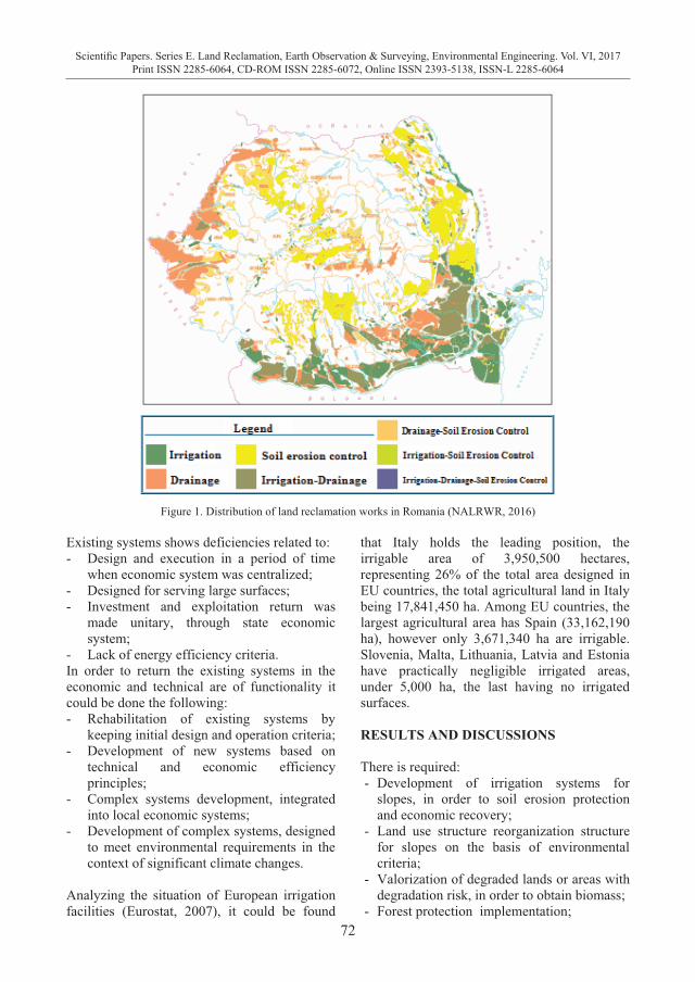
72
Scientific Papers. Series E. Land Reclamation, Earth Observation & Surveying, Environmental Engineering. Vol. VI, 2017Print ISSN 2285-6064, CD-ROM ISSN 2285-6072, Online ISSN 2393-5138, ISSN-L 2285-6064
Figure 1. Distribution of land reclamation works in Romania (NALRWR, 2016)
Existing systems shows deficiencies related to: - Design and execution in a period of time
when economic system was centralized; - Designed for serving large surfaces; - Investment and exploitation return was
made unitary, through state economic system;
- Lack of energy efficiency criteria. In order to return the existing systems in the economic and technical are of functionality it could be done the following: - Rehabilitation of existing systems by
keeping initial design and operation criteria; - Development of new systems based on
technical and economic efficiency principles;
- Complex systems development, integrated into local economic systems;
- Development of complex systems, designed to meet environmental requirements in the context of significant climate changes.
Analyzing the situation of European irrigation facilities (Eurostat, 2007), it could be found
that Italy holds the leading position, the irrigable area of 3,950,500 hectares, representing 26% of the total area designed in EU countries, the total agricultural land in Italy being 17,841,450 ha. Among EU countries, the largest agricultural area has Spain (33,162,190 ha), however only 3,671,340 ha are irrigable. Slovenia, Malta, Lithuania, Latvia and Estonia have practically negligible irrigated areas, under 5,000 ha, the last having no irrigated surfaces. RESULTS AND DISCUSSIONS There is required: - Development of irrigation systems for
slopes, in order to soil erosion protection and economic recovery;
- Land use structure reorganization structure for slopes on the basis of environmental criteria;
- Valorization of degraded lands or areas with degradation risk, in order to obtain biomass;
- Forest protection implementation;
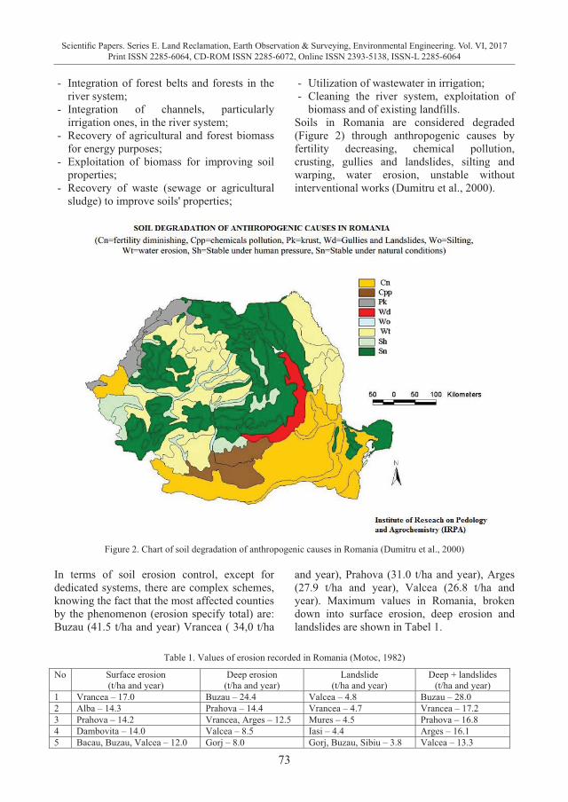
73
Scientific Papers. Series E. Land Reclamation, Earth Observation & Surveying, Environmental Engineering. Vol. VI, 2017Print ISSN 2285-6064, CD-ROM ISSN 2285-6072, Online ISSN 2393-5138, ISSN-L 2285-6064
Figure 1. Distribution of land reclamation works in Romania (NALRWR, 2016)
Existing systems shows deficiencies related to: - Design and execution in a period of time
when economic system was centralized; - Designed for serving large surfaces; - Investment and exploitation return was
made unitary, through state economic system;
- Lack of energy efficiency criteria. In order to return the existing systems in the economic and technical are of functionality it could be done the following: - Rehabilitation of existing systems by
keeping initial design and operation criteria; - Development of new systems based on
technical and economic efficiency principles;
- Complex systems development, integrated into local economic systems;
- Development of complex systems, designed to meet environmental requirements in the context of significant climate changes.
Analyzing the situation of European irrigation facilities (Eurostat, 2007), it could be found
that Italy holds the leading position, the irrigable area of 3,950,500 hectares, representing 26% of the total area designed in EU countries, the total agricultural land in Italy being 17,841,450 ha. Among EU countries, the largest agricultural area has Spain (33,162,190 ha), however only 3,671,340 ha are irrigable. Slovenia, Malta, Lithuania, Latvia and Estonia have practically negligible irrigated areas, under 5,000 ha, the last having no irrigated surfaces. RESULTS AND DISCUSSIONS There is required: - Development of irrigation systems for
slopes, in order to soil erosion protection and economic recovery;
- Land use structure reorganization structure for slopes on the basis of environmental criteria;
- Valorization of degraded lands or areas with degradation risk, in order to obtain biomass;
- Forest protection implementation;
- Integration of forest belts and forests in the river system;
- Integration of channels, particularly irrigation ones, in the river system;
- Recovery of agricultural and forest biomass for energy purposes;
- Exploitation of biomass for improving soil properties;
- Recovery of waste (sewage or agricultural sludge) to improve soils' properties;
- Utilization of wastewater in irrigation; - Cleaning the river system, exploitation of
biomass and of existing landfills. Soils in Romania are considered degraded (Figure 2) through anthropogenic causes by fertility decreasing, chemical pollution, crusting, gullies and landslides, silting and warping, water erosion, unstable without interventional works (Dumitru et al., 2000).
Figure 2. Chart of soil degradation of anthropogenic causes in Romania (Dumitru et al., 2000)
In terms of soil erosion control, except for dedicated systems, there are complex schemes, knowing the fact that the most affected counties by the phenomenon (erosion specify total) are: Buzau (41.5 t/ha and year) Vrancea ( 34,0 t/ha
and year), Prahova (31.0 t/ha and year), Arges (27.9 t/ha and year), Valcea (26.8 t/ha and year). Maximum values in Romania, broken down into surface erosion, deep erosion and landslides are shown in Tabel 1.
Table 1. Values of erosion recorded in Romania (Motoc, 1982)
No Surface erosion (t/ha and year)
Deep erosion (t/ha and year)
Landslide (t/ha and year)
Deep + landslides (t/ha and year)
1 Vrancea – 17.0 Buzau – 24.4 Valcea – 4.8 Buzau – 28.0 2 Alba – 14.3 Prahova – 14.4 Vrancea – 4.7 Vrancea – 17.2 3 Prahova – 14.2 Vrancea, Arges – 12.5 Mures – 4.5 Prahova – 16.8 4 Dambovita – 14.0 Valcea – 8.5 Iasi – 4.4 Arges – 16.1 5 Bacau, Buzau, Valcea – 12.0 Gorj – 8.0 Gorj, Buzau, Sibiu – 3.8 Valcea – 13.3
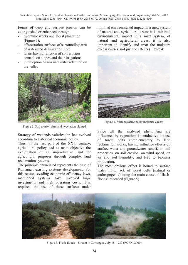
74
Scientific Papers. Series E. Land Reclamation, Earth Observation & Surveying, Environmental Engineering. Vol. VI, 2017Print ISSN 2285-6064, CD-ROM ISSN 2285-6072, Online ISSN 2393-5138, ISSN-L 2285-6064
Forms of deep and surface erosion can be extinguished or enhanced through: - hydraulic works and forest plantation
(Figure 3); - afforestation surfaces of surrounding area
of watershed delimitation line; - farms having function of soil erosion
control on slopes and their irrigation; - interception basins and water retention on
the valley.
Figure 3. Soil erosion dam and vegetation planted
Strategy of wetlands valorization has evolved according to historical economic policy. Thus, in the last part of the XXth century, agricultural policy had as main objective the exploitation of all unproductive land for agricultural purposes through complex land reclamation systems. The principle enunciated represents the base of Romanian existing systems development. For this reason, evading economic efficiency laws, mentioned systems have involved large investments and high operating costs. It is required the use of these surfaces under
minimal environmental impact in a mixt system of natural and agricultural areas; it is minimal environmental impact in a mixt system, of natural and agricultural areas; it is also important to identify and treat the moisture excess causes, not just the effects (Figure 4)
Figure 4. Surfaces affected by moisture excess
Since all the analyzed phenomena are influenced by vegetation, is conductive the use of forest belts complementary to land reclamation works, having influence effects on surface water and groundwater runoff, on soil properties, on soil erosion, on wind speed, on air and soil humidity, and lead to biomass production. The most obvious effect is bound to surface water flow, lack of forest belts (natural or anthropogenic) being the main cause of “flash-floods” recorded (Figure 5).
Figure 5. Flash-floods – Stream in Zavraggia, July 18, 1987 (FOEN, 2000)
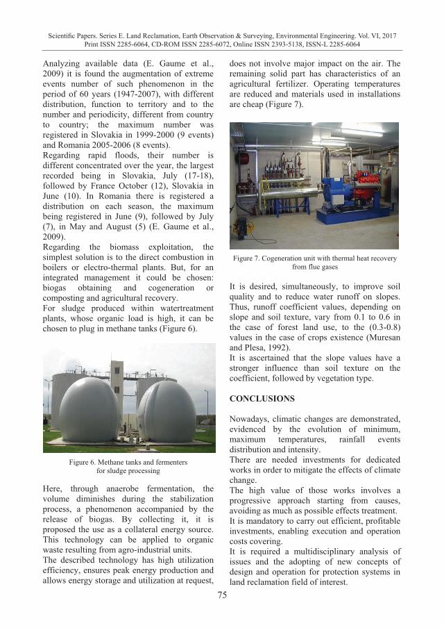
75
Scientific Papers. Series E. Land Reclamation, Earth Observation & Surveying, Environmental Engineering. Vol. VI, 2017Print ISSN 2285-6064, CD-ROM ISSN 2285-6072, Online ISSN 2393-5138, ISSN-L 2285-6064
Forms of deep and surface erosion can be extinguished or enhanced through: - hydraulic works and forest plantation
(Figure 3); - afforestation surfaces of surrounding area
of watershed delimitation line; - farms having function of soil erosion
control on slopes and their irrigation; - interception basins and water retention on
the valley.
Figure 3. Soil erosion dam and vegetation planted
Strategy of wetlands valorization has evolved according to historical economic policy. Thus, in the last part of the XXth century, agricultural policy had as main objective the exploitation of all unproductive land for agricultural purposes through complex land reclamation systems. The principle enunciated represents the base of Romanian existing systems development. For this reason, evading economic efficiency laws, mentioned systems have involved large investments and high operating costs. It is required the use of these surfaces under
minimal environmental impact in a mixt system of natural and agricultural areas; it is minimal environmental impact in a mixt system, of natural and agricultural areas; it is also important to identify and treat the moisture excess causes, not just the effects (Figure 4)
Figure 4. Surfaces affected by moisture excess
Since all the analyzed phenomena are influenced by vegetation, is conductive the use of forest belts complementary to land reclamation works, having influence effects on surface water and groundwater runoff, on soil properties, on soil erosion, on wind speed, on air and soil humidity, and lead to biomass production. The most obvious effect is bound to surface water flow, lack of forest belts (natural or anthropogenic) being the main cause of “flash-floods” recorded (Figure 5).
Figure 5. Flash-floods – Stream in Zavraggia, July 18, 1987 (FOEN, 2000)
Analyzing available data (E. Gaume et al., 2009) it is found the augmentation of extreme events number of such phenomenon in the period of 60 years (1947-2007), with different distribution, function to territory and to the number and periodicity, different from country to country; the maximum number was registered in Slovakia in 1999-2000 (9 events) and Romania 2005-2006 (8 events). Regarding rapid floods, their number is different concentrated over the year, the largest recorded being in Slovakia, July (17-18), followed by France October (12), Slovakia in June (10). In Romania there is registered a distribution on each season, the maximum being registered in June (9), followed by July (7), in May and August (5) (E. Gaume et al., 2009). Regarding the biomass exploitation, the simplest solution is to the direct combustion in boilers or electro-thermal plants. But, for an integrated management it could be chosen: biogas obtaining and cogeneration or composting and agricultural recovery. For sludge produced within watertreatment plants, whose organic load is high, it can be chosen to plug in methane tanks (Figure 6).
Figure 6. Methane tanks and fermenters
for sludge processing
Here, through anaerobe fermentation, the volume diminishes during the stabilization process, a phenomenon accompanied by the release of biogas. By collecting it, it is proposed the use as a collateral energy source. This technology can be applied to organic waste resulting from agro-industrial units. The described technology has high utilization efficiency, ensures peak energy production and allows energy storage and utilization at request,
does not involve major impact on the air. The remaining solid part has characteristics of an agricultural fertilizer. Operating temperatures are reduced and materials used in installations are cheap (Figure 7).
Figure 7. Cogeneration unit with thermal heat recovery
from flue gases It is desired, simultaneously, to improve soil quality and to reduce water runoff on slopes. Thus, runoff coefficient values, depending on slope and soil texture, vary from 0.1 to 0.6 in the case of forest land use, to the (0.3-0.8) values in the case of crops existence (Muresan and Plesa, 1992). It is ascertained that the slope values have a stronger influence than soil texture on the coefficient, followed by vegetation type. CONCLUSIONS Nowadays, climatic changes are demonstrated, evidenced by the evolution of minimum, maximum temperatures, rainfall events distribution and intensity. There are needed investments for dedicated works in order to mitigate the effects of climate change. The high value of those works involves a progressive approach starting from causes, avoiding as much as possible effects treatment. It is mandatory to carry out efficient, profitable investments, enabling execution and operation costs covering. It is required a multidisciplinary analysis of issues and the adopting of new concepts of design and operation for protection systems in land reclamation field of interest.

76
Scientific Papers. Series E. Land Reclamation, Earth Observation & Surveying, Environmental Engineering. Vol. VI, 2017Print ISSN 2285-6064, CD-ROM ISSN 2285-6072, Online ISSN 2393-5138, ISSN-L 2285-6064
REFERENCES Dumitru M., Ciobanu C., Motelica D.M., Mashali A.M.,
Elisabeta Dumitru,. Cojocaru G, Roxana Enache, Eugenia Gamenţ, Doina Plaxienco, Cristina Radnea, Cârstea St., Alexandrina Manea, Nicoleta Vrînceanu, Calciu I., 2000., Monitoring of Soil Quality in Romania (Bilingual Atlas - Romanian and English), GNP Publishing House, Bucharest, 102.
Gaume E. et al., 2009, A compilation of data on European flash floods, Journal of Hydrology 367, 70–78.
Motoc M., 1982, The average rate of erosion degradation of soil in S.R. of Romania, Newsletter, ASAS Journal No. 12, Bucharest.
Muresan D., Plesa I., 1992, Irrigation, drainage and soil erosion control, EDP Publishing House, Bucharest, 65.
National Administration for Land Reclamation Works, Romania (NALRWR), 2016, www.anif.ro/ patrimoniu/ imbunatatiri-funciare.htm
Swiss Federal Office for the Environment – FOEN, 2000 https://www.google.ro/search?q=swiss+federal+office+for+the+environment+foen&client=firefox-b&source=lnms&tbm=isch&sa=X&ved=0ahUKEwj5obKLjd3SAhVHuBQKHZHdCjEQ_AUICCgB&biw=1252&bih=602#imgrc=9QPgK8lbGNjFqM:
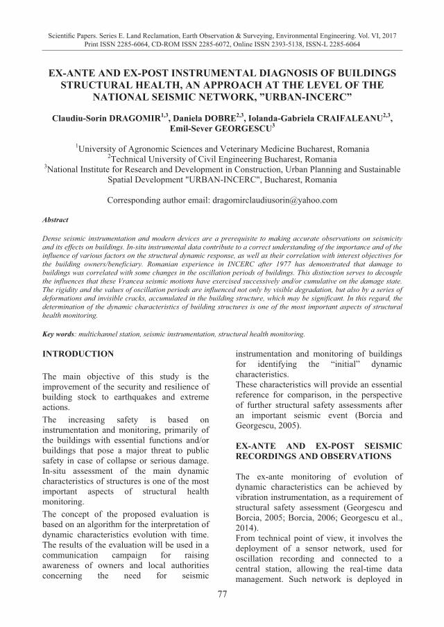
77
Scientific Papers. Series E. Land Reclamation, Earth Observation & Surveying, Environmental Engineering. Vol. VI, 2017Print ISSN 2285-6064, CD-ROM ISSN 2285-6072, Online ISSN 2393-5138, ISSN-L 2285-6064
REFERENCES Dumitru M., Ciobanu C., Motelica D.M., Mashali A.M.,
Elisabeta Dumitru,. Cojocaru G, Roxana Enache, Eugenia Gamenţ, Doina Plaxienco, Cristina Radnea, Cârstea St., Alexandrina Manea, Nicoleta Vrînceanu, Calciu I., 2000., Monitoring of Soil Quality in Romania (Bilingual Atlas - Romanian and English), GNP Publishing House, Bucharest, 102.
Gaume E. et al., 2009, A compilation of data on European flash floods, Journal of Hydrology 367, 70–78.
Motoc M., 1982, The average rate of erosion degradation of soil in S.R. of Romania, Newsletter, ASAS Journal No. 12, Bucharest.
Muresan D., Plesa I., 1992, Irrigation, drainage and soil erosion control, EDP Publishing House, Bucharest, 65.
National Administration for Land Reclamation Works, Romania (NALRWR), 2016, www.anif.ro/ patrimoniu/ imbunatatiri-funciare.htm
Swiss Federal Office for the Environment – FOEN, 2000 https://www.google.ro/search?q=swiss+federal+office+for+the+environment+foen&client=firefox-b&source=lnms&tbm=isch&sa=X&ved=0ahUKEwj5obKLjd3SAhVHuBQKHZHdCjEQ_AUICCgB&biw=1252&bih=602#imgrc=9QPgK8lbGNjFqM:
EX-ANTE AND EX-POST INSTRUMENTAL DIAGNOSIS OF BUILDINGS
STRUCTURAL HEALTH, AN APPROACH AT THE LEVEL OF THE NATIONAL SEISMIC NETWORK, ”URBAN-INCERC”
Claudiu-Sorin DRAGOMIR1,3, Daniela DOBRE2,3, Iolanda-Gabriela CRAIFALEANU2,3,
Emil-Sever GEORGESCU3
1University of Agronomic Sciences and Veterinary Medicine Bucharest, Romania 2Technical University of Civil Engineering Bucharest, Romania
3National Institute for Research and Development in Construction, Urban Planning and Sustainable Spatial Development "URBAN-INCERC", Bucharest, Romania
Corresponding author email: [email protected]
Abstract Dense seismic instrumentation and modern devices are a prerequisite to making accurate observations on seismicity and its effects on buildings. In-situ instrumental data contribute to a correct understanding of the importance and of the influence of various factors on the structural dynamic response, as well as their correlation with interest objectives for the building owners/beneficiary. Romanian experience in INCERC after 1977 has demonstrated that damage to buildings was correlated with some changes in the oscillation periods of buildings. This distinction serves to decouple the influences that these Vrancea seismic motions have exercised successively and/or cumulative on the damage state. The rigidity and the values of oscillation periods are influenced not only by visible degradation, but also by a series of deformations and invisible cracks, accumulated in the building structure, which may be significant. In this regard, the determination of the dynamic characteristics of building structures is one of the most important aspects of structural health monitoring. Key words: multichannel station, seismic instrumentation, structural health monitoring. INTRODUCTION The main objective of this study is the improvement of the security and resilience of building stock to earthquakes and extreme actions. The increasing safety is based on instrumentation and monitoring, primarily of the buildings with essential functions and/or buildings that pose a major threat to public safety in case of collapse or serious damage. In-situ assessment of the main dynamic characteristics of structures is one of the most important aspects of structural health monitoring. The concept of the proposed evaluation is based on an algorithm for the interpretation of dynamic characteristics evolution with time. The results of the evaluation will be used in a communication campaign for raising awareness of owners and local authorities concerning the need for seismic
instrumentation and monitoring of buildings for identifying the “initial” dynamic characteristics. These characteristics will provide an essential reference for comparison, in the perspective of further structural safety assessments after an important seismic event (Borcia and Georgescu, 2005). EX-ANTE AND EX-POST SEISMIC RECORDINGS AND OBSERVATIONS The ex-ante monitoring of evolution of dynamic characteristics can be achieved by vibration instrumentation, as a requirement of structural safety assessment (Georgescu and Borcia, 2005; Borcia, 2006; Georgescu et al., 2014). From technical point of view, it involves the deployment of a sensor network, used for oscillation recording and connected to a central station, allowing the real-time data management. Such network is deployed in
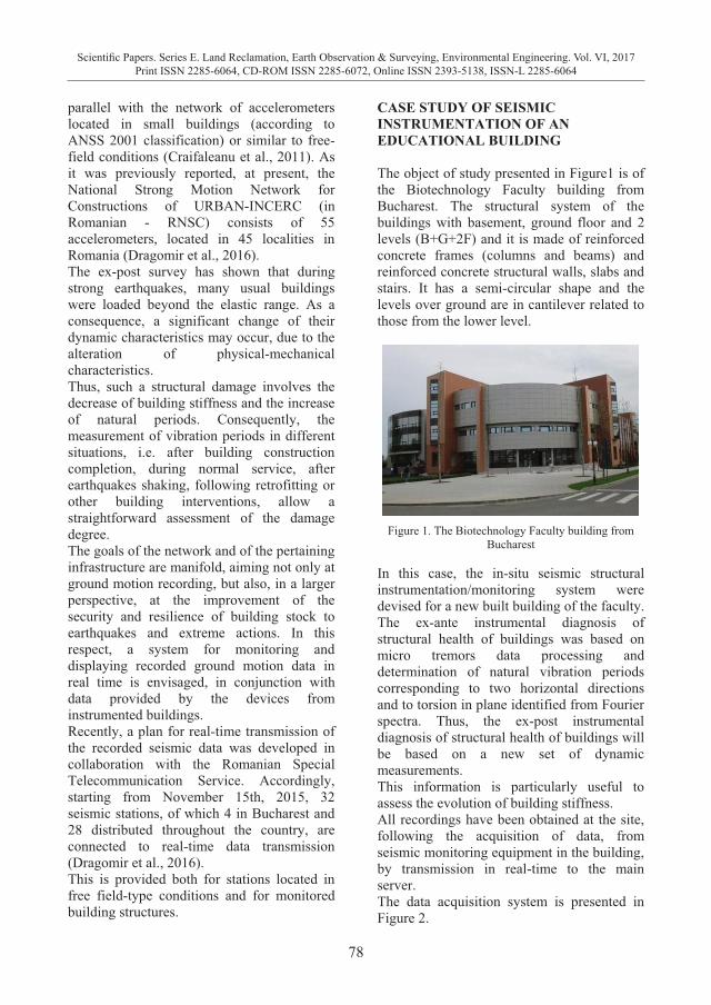
78
Scientific Papers. Series E. Land Reclamation, Earth Observation & Surveying, Environmental Engineering. Vol. VI, 2017Print ISSN 2285-6064, CD-ROM ISSN 2285-6072, Online ISSN 2393-5138, ISSN-L 2285-6064
parallel with the network of accelerometers located in small buildings (according to ANSS 2001 classification) or similar to free-field conditions (Craifaleanu et al., 2011). As it was previously reported, at present, the National Strong Motion Network for Constructions of URBAN-INCERC (in Romanian - RNSC) consists of 55 accelerometers, located in 45 localities in Romania (Dragomir et al., 2016). The ex-post survey has shown that during strong earthquakes, many usual buildings were loaded beyond the elastic range. As a consequence, a significant change of their dynamic characteristics may occur, due to the alteration of physical-mechanical characteristics. Thus, such a structural damage involves the decrease of building stiffness and the increase of natural periods. Consequently, the measurement of vibration periods in different situations, i.e. after building construction completion, during normal service, after earthquakes shaking, following retrofitting or other building interventions, allow a straightforward assessment of the damage degree. The goals of the network and of the pertaining infrastructure are manifold, aiming not only at ground motion recording, but also, in a larger perspective, at the improvement of the security and resilience of building stock to earthquakes and extreme actions. In this respect, a system for monitoring and displaying recorded ground motion data in real time is envisaged, in conjunction with data provided by the devices from instrumented buildings. Recently, a plan for real-time transmission of the recorded seismic data was developed in collaboration with the Romanian Special Telecommunication Service. Accordingly, starting from November 15th, 2015, 32 seismic stations, of which 4 in Bucharest and 28 distributed throughout the country, are connected to real-time data transmission (Dragomir et al., 2016). This is provided both for stations located in free field-type conditions and for monitored building structures.
CASE STUDY OF SEISMIC INSTRUMENTATION OF AN EDUCATIONAL BUILDING The object of study presented in Figure1 is of the Biotechnology Faculty building from Bucharest. The structural system of the buildings with basement, ground floor and 2 levels (B+G+2F) and it is made of reinforced concrete frames (columns and beams) and reinforced concrete structural walls, slabs and stairs. It has a semi-circular shape and the levels over ground are in cantilever related to those from the lower level.
Figure 1. The Biotechnology Faculty building from
Bucharest
In this case, the in-situ seismic structural instrumentation/monitoring system were devised for a new built building of the faculty. The ex-ante instrumental diagnosis of structural health of buildings was based on micro tremors data processing and determination of natural vibration periods corresponding to two horizontal directions and to torsion in plane identified from Fourier spectra. Thus, the ex-post instrumental diagnosis of structural health of buildings will be based on a new set of dynamic measurements. This information is particularly useful to assess the evolution of building stiffness. All recordings have been obtained at the site, following the acquisition of data, from seismic monitoring equipment in the building, by transmission in real-time to the main server. The data acquisition system is presented in Figure 2.
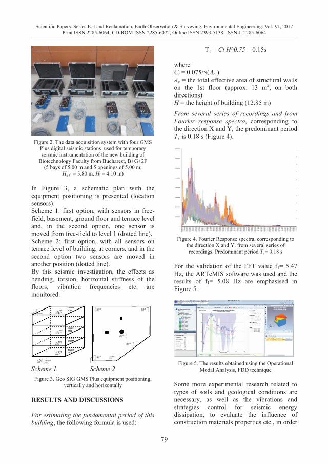
79
Scientific Papers. Series E. Land Reclamation, Earth Observation & Surveying, Environmental Engineering. Vol. VI, 2017Print ISSN 2285-6064, CD-ROM ISSN 2285-6072, Online ISSN 2393-5138, ISSN-L 2285-6064
parallel with the network of accelerometers located in small buildings (according to ANSS 2001 classification) or similar to free-field conditions (Craifaleanu et al., 2011). As it was previously reported, at present, the National Strong Motion Network for Constructions of URBAN-INCERC (in Romanian - RNSC) consists of 55 accelerometers, located in 45 localities in Romania (Dragomir et al., 2016). The ex-post survey has shown that during strong earthquakes, many usual buildings were loaded beyond the elastic range. As a consequence, a significant change of their dynamic characteristics may occur, due to the alteration of physical-mechanical characteristics. Thus, such a structural damage involves the decrease of building stiffness and the increase of natural periods. Consequently, the measurement of vibration periods in different situations, i.e. after building construction completion, during normal service, after earthquakes shaking, following retrofitting or other building interventions, allow a straightforward assessment of the damage degree. The goals of the network and of the pertaining infrastructure are manifold, aiming not only at ground motion recording, but also, in a larger perspective, at the improvement of the security and resilience of building stock to earthquakes and extreme actions. In this respect, a system for monitoring and displaying recorded ground motion data in real time is envisaged, in conjunction with data provided by the devices from instrumented buildings. Recently, a plan for real-time transmission of the recorded seismic data was developed in collaboration with the Romanian Special Telecommunication Service. Accordingly, starting from November 15th, 2015, 32 seismic stations, of which 4 in Bucharest and 28 distributed throughout the country, are connected to real-time data transmission (Dragomir et al., 2016). This is provided both for stations located in free field-type conditions and for monitored building structures.
CASE STUDY OF SEISMIC INSTRUMENTATION OF AN EDUCATIONAL BUILDING The object of study presented in Figure1 is of the Biotechnology Faculty building from Bucharest. The structural system of the buildings with basement, ground floor and 2 levels (B+G+2F) and it is made of reinforced concrete frames (columns and beams) and reinforced concrete structural walls, slabs and stairs. It has a semi-circular shape and the levels over ground are in cantilever related to those from the lower level.
Figure 1. The Biotechnology Faculty building from
Bucharest
In this case, the in-situ seismic structural instrumentation/monitoring system were devised for a new built building of the faculty. The ex-ante instrumental diagnosis of structural health of buildings was based on micro tremors data processing and determination of natural vibration periods corresponding to two horizontal directions and to torsion in plane identified from Fourier spectra. Thus, the ex-post instrumental diagnosis of structural health of buildings will be based on a new set of dynamic measurements. This information is particularly useful to assess the evolution of building stiffness. All recordings have been obtained at the site, following the acquisition of data, from seismic monitoring equipment in the building, by transmission in real-time to the main server. The data acquisition system is presented in Figure 2.
Figure 2. The data acquisition system with four GMS
Plus digital seismic stations used for temporary seismic instrumentation of the new building of
Biotechnology Faculty from Bucharest, B+G+2F (5 bays of 5.00 m and 5 openings of 5.00 m;
Hg f = 3.80 m, Hl = 4.10 m) In Figure 3, a schematic plan with the equipment positioning is presented (location sensors). Scheme 1: first option, with sensors in free-field, basement, ground floor and terrace level and, in the second option, one sensor is moved from free-field to level 1 (dotted line). Scheme 2: first option, with all sensors on terrace level of building, at corners, and in the second option two sensors are moved in another position (dotted line). By this seismic investigation, the effects as bending, torsion, horizontal stiffness of the floors; vibration frequencies etc. are monitored.
Scheme 1 Scheme 2
Figure 3. Geo SIG GMS Plus equipment positioning, vertically and horizontally
RESULTS AND DISCUSSIONS For estimating the fundamental period of this building, the following formula is used:
T1 = Ct H^0.75 = 0.15s where Ct = 0.075/√(Ac ) Ac = the total effective area of structural walls on the 1st floor (approx. 13 m2, on both directions) H = the height of building (12.85 m) From several series of recordings and from Fourier response spectra, corresponding to the direction X and Y, the predominant period T1 is 0.18 s (Figure 4).
Figure 4. Fourier Response spectra, corresponding to
the direction X and Y, from several series of recordings. Predominant period T1= 0.18 s
For the validation of the FFT value f1= 5.47 Hz, the ARTeMIS software was used and the results of f1= 5.08 Hz are emphasised in Figure 5.
Figure 5. The results obtained using the Operational
Modal Analysis, FDD technique Some more experimental research related to types of soils and geological conditions are necessary, as well as the vibrations and strategies control for seismic energy dissipation, to evaluate the influence of construction materials properties etc., in order
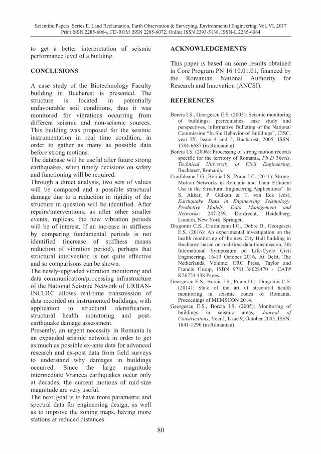
80
Scientific Papers. Series E. Land Reclamation, Earth Observation & Surveying, Environmental Engineering. Vol. VI, 2017Print ISSN 2285-6064, CD-ROM ISSN 2285-6072, Online ISSN 2393-5138, ISSN-L 2285-6064
to get a better interpretation of seismic performance level of a building. CONCLUSIONS A case study of the Biotechnology Faculty building in Bucharest is presented. The structure is located in potentially unfavourable soil conditions, thus it was monitored for vibrations occurring from different seismic and non-seismic sources. This building was proposed for the seismic instrumentation in real time condition, in order to gather as many as possible data before strong motions. The database will be useful after future strong earthquakes, when timely decisions on safety and functioning will be required. Through a direct analysis, two sets of values will be compared and a possible structural damage due to a reduction in rigidity of the structure in question will be identified. After repairs/interventions, as after other smaller events, replicas, the new vibration periods will be of interest. If an increase in stiffness by comparing fundamental periods is not identified (increase of stiffness means reduction of vibration period), perhaps that structural intervention is not quite effective and so comparisons can be shown. The newly-upgraded vibration monitoring and data communication/processing infrastructure of the National Seismic Network of URBAN-INCERC allows real-time transmission of data recorded on instrumented buildings, with application to structural identification, structural health monitoring and post-earthquake damage assessment. Presently, an urgent necessity in Romania is an expanded seismic network in order to get as much as possible ex-ante data for advanced research and ex-post data from field surveys to understand why damages in buildings occurred. Since the large magnitude intermediate Vrancea earthquakes occur only at decades, the current motions of mid-size magnitude are very useful. The next goal is to have more parametric and spectral data for engineering design, as well as to improve the zoning maps, having more stations at reduced distances.
ACKNOWLEDGEMENTS This paper is based on some results obtained in Core Program PN 16 10.01.01, financed by the Romanian National Authority for Research and Innovation (ANCSI). REFERENCES Borcia I.S., Georgescu E.S. (2005): Seismic monitoring
of buildings: prerequisites, case study and perspectives, Informative Bulleting of the National Commission “In Siu Behavior of Buildings”, CISC, year IX, Issue 4 and 5, Bucharest, 2005, ISSN: 1584-6687 (in Romanian).
Borcia I.S. (2006): Processing of strong motion records specific for the territory of Romania, Ph D Thesis, Technical University of Civil Engineering, Bucharest, Romania.
Craifaleanu I.G., Borcia I.S., Praun I.C. (2011): Strong-Motion Networks in Romania and Their Efficient Use in the Structural Engineering Applications”. In S. Akkar, P. Gülkan & T. van Eck (eds), Earthquake Data in Engineering Seismology. Predictive Models, Data Management and Networks: 247-259. Dordrecht, Heidelberg, London, New York: Springer.
Dragomir C.S., Craifaleanu I.G., Dobre D., Georgescu E.S. (2016): An experimental investigation on the health monitoring of the new City Hall building in Bucharest based on real-time data transmission, 5th International Symposium on Life-Cycle Civil Engineering, 16-19 October 2016, At Delft, The Netherlands, Volume: CRC Press, Taylor and Francis Group, ISBN 9781138028470 - CAT# K26754 438 Pages.
Georgescu E.S., Borcia I.S., Praun I.C., Dragomir C.S. (2014): State of the art of structural health monitoring in seismic zones of Romania, Proceedings of MEMSCON 2014.
Georgescu E.S., Borcia I.S. (2005): Monitoring of buildings in seismic areas, Journal of Constructions, Year I, Issue 9, October 2005, ISSN: 1841-1290 (in Romanian).
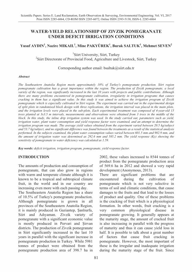
81
Scientific Papers. Series E. Land Reclamation, Earth Observation & Surveying, Environmental Engineering. Vol. VI, 2017Print ISSN 2285-6064, CD-ROM ISSN 2285-6072, Online ISSN 2393-5138, ISSN-L 2285-6064
to get a better interpretation of seismic performance level of a building. CONCLUSIONS A case study of the Biotechnology Faculty building in Bucharest is presented. The structure is located in potentially unfavourable soil conditions, thus it was monitored for vibrations occurring from different seismic and non-seismic sources. This building was proposed for the seismic instrumentation in real time condition, in order to gather as many as possible data before strong motions. The database will be useful after future strong earthquakes, when timely decisions on safety and functioning will be required. Through a direct analysis, two sets of values will be compared and a possible structural damage due to a reduction in rigidity of the structure in question will be identified. After repairs/interventions, as after other smaller events, replicas, the new vibration periods will be of interest. If an increase in stiffness by comparing fundamental periods is not identified (increase of stiffness means reduction of vibration period), perhaps that structural intervention is not quite effective and so comparisons can be shown. The newly-upgraded vibration monitoring and data communication/processing infrastructure of the National Seismic Network of URBAN-INCERC allows real-time transmission of data recorded on instrumented buildings, with application to structural identification, structural health monitoring and post-earthquake damage assessment. Presently, an urgent necessity in Romania is an expanded seismic network in order to get as much as possible ex-ante data for advanced research and ex-post data from field surveys to understand why damages in buildings occurred. Since the large magnitude intermediate Vrancea earthquakes occur only at decades, the current motions of mid-size magnitude are very useful. The next goal is to have more parametric and spectral data for engineering design, as well as to improve the zoning maps, having more stations at reduced distances.
ACKNOWLEDGEMENTS This paper is based on some results obtained in Core Program PN 16 10.01.01, financed by the Romanian National Authority for Research and Innovation (ANCSI). REFERENCES Borcia I.S., Georgescu E.S. (2005): Seismic monitoring
of buildings: prerequisites, case study and perspectives, Informative Bulleting of the National Commission “In Siu Behavior of Buildings”, CISC, year IX, Issue 4 and 5, Bucharest, 2005, ISSN: 1584-6687 (in Romanian).
Borcia I.S. (2006): Processing of strong motion records specific for the territory of Romania, Ph D Thesis, Technical University of Civil Engineering, Bucharest, Romania.
Craifaleanu I.G., Borcia I.S., Praun I.C. (2011): Strong-Motion Networks in Romania and Their Efficient Use in the Structural Engineering Applications”. In S. Akkar, P. Gülkan & T. van Eck (eds), Earthquake Data in Engineering Seismology. Predictive Models, Data Management and Networks: 247-259. Dordrecht, Heidelberg, London, New York: Springer.
Dragomir C.S., Craifaleanu I.G., Dobre D., Georgescu E.S. (2016): An experimental investigation on the health monitoring of the new City Hall building in Bucharest based on real-time data transmission, 5th International Symposium on Life-Cycle Civil Engineering, 16-19 October 2016, At Delft, The Netherlands, Volume: CRC Press, Taylor and Francis Group, ISBN 9781138028470 - CAT# K26754 438 Pages.
Georgescu E.S., Borcia I.S., Praun I.C., Dragomir C.S. (2014): State of the art of structural health monitoring in seismic zones of Romania, Proceedings of MEMSCON 2014.
Georgescu E.S., Borcia I.S. (2005): Monitoring of buildings in seismic areas, Journal of Constructions, Year I, Issue 9, October 2005, ISSN: 1841-1290 (in Romanian).
WATER-YIELD RELATIONSHIP OF ZIVZIK POMEGRANATE
UNDER DEFICIT IRRIGATION CONDITIONS
Yusuf AYDIN1, Nazire MIKAIL1, Mine PAKYÜREK1, Burak SALTUK1, Mehmet SEVEN2
1Siirt University, Siirt, Turkey
2Siirt Directorate of Provincial Food, Agriculture and Livestock, Siirt, Turkey
Corresponding author email: [email protected]
Abstract The Southeastern Anatolia Region meets approximately 10% of Turkey's pomegranate production. Siirt region pomegranate cultivation has a great importance within the region. The production of Zivzik pomegranate, a local variety of the region, was significantly increased in the last 10 years with projects and public contributions. Although there are many problems encountered in pomegranate cultivation, irregularity in irrigation programs that causes cracking in them has a significant value. In this study it was aimed to achieve the irrigation program of Zivzik pomegranate which is especially cultivated in Siirt region. The experiment was carried out in the experimental design of split plots in randomised block design with three replications, the irrigation interval was placed in the main plots, and the irrigation levels were placed in the sub-plots. Each experimental treatment was composed of 4-year-old 15 trees planted at 3x3.5 m intervals, measurements and observations were obtained from 3 trees in the middle of the block. In this study, the inline drip irrigation system was used. In the study carried out, parameters such as yield, irrigation water, plant water consumption and yield response factor were examined, and an attempt to determine the irrigation program was made. The average yield values obtained from the experiment varied between 20.5 kg/subject and 53.7 kg/subject, and no significant difference was found between the treatments as a result of the statistical analysis performed. In the subjects examined, the plant water consumption values varied between 601.5 mm and 902.9 mm, and the amount of irrigation water was determined as 292.6 mm and 585.2 mm. The yield response (Ky) showing the sensitivity of pomegranate to water deficiency was calculated as 1.59. Key words: deficit irrigation, irrigation program, pomegranate, yield response factor.
INTRODUCTION The amounts of production and consumption of pomegranate, that can also grow in regions with warm and temperate climate although it is known to be a tropical and subtropical climate fruit, in the world and in our country are increasing even more with each passing day. The Southeastern Anatolia Region has a share of 10.5% of Turkey's pomegranate production. Although pomegranate is grown in all provinces of the Southeastern Anatolia Region, it is mainly produced in Gaziantep, Şanlıurfa, Siirt and Adıyaman. Zivzik variety of pomegranate with a significant economic value is mostly produced in Pervari and Şirvan districts. The production of Zivzik pomegranate in Siirt significantly increased in the last 10 years in parallel with the significant increase in pomegranate production in Turkey. While 5981 tonnes of product were obtained from the pomegranate production area of 398.7 ha in
2002, these values increased to 8544 tonnes of product from the pomegranate production area of 569.6 ha in 2012 and showed a very rapid development (Anonymous, 2013). There are significant problems that are encountered during the cultivation of pomegranate which is not very selective in terms of soil and climatic conditions, that cause damages to the fruits and that lead to the losses of product and quality. One of these problems is the cracking of fruit which is a physiological formation. In other words, fruit cracking is a very common physiological disease in pomegranate growing. It generally appears at the maturity stage, the amount of cracked fruit is also increasing in parallel with the progress of maturity and thus it can cause yield loss in half. It is possible to talk about a great number of factors that cause fruit cracking in pomegranate. However, the most important of these is the irregular and inadequate irrigation during the maturity stage of the fruit. Since
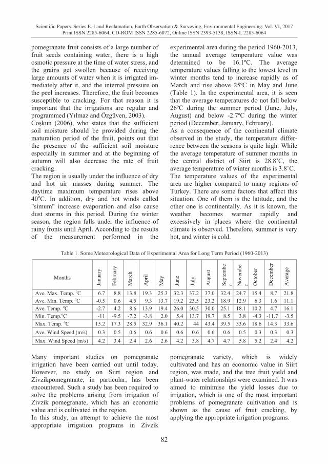
82
Scientific Papers. Series E. Land Reclamation, Earth Observation & Surveying, Environmental Engineering. Vol. VI, 2017Print ISSN 2285-6064, CD-ROM ISSN 2285-6072, Online ISSN 2393-5138, ISSN-L 2285-6064
pomegranate fruit consists of a large number of fruit seeds containing water, there is a high osmotic pressure at the time of water stress, and the grains get swollen because of receiving large amounts of water when it is irrigated im-mediately after it, and the internal pressure on the peel increases. Therefore, the fruit becomes susceptible to cracking. For that reason it is important that the irrigations are regular and programmed (Yılmaz and Özgüven, 2003). Coşkun (2006), who states that the sufficient soil moisture should be provided during the maturation period of the fruit, points out that the presence of the sufficient soil moisture especially in summer and at the beginning of autumn will also decrease the rate of fruit cracking. The region is usually under the influence of dry and hot air masses during summer. The daytime maximum temperature rises above 40oC. In addition, dry and hot winds called "simum" increase evaporation and also cause dust storms in this period. During the winter season, the region falls under the influence of rainy fronts until April. According to the results of the measurement performed in the
experimental area during the period 1960-2013, the annual average temperature value was determined to be 16.1ºC. The average temperature values falling to the lowest level in winter months tend to increase rapidly as of March and rise above 25ºC in May and June (Table 1). In the experimental area, it is seen that the average temperatures do not fall below 26ºC during the summer period (June, July, August) and below -2.7ºC during the winter period (December, January, February). As a consequence of the continental climate observed in the study, the temperature differ-rence between the seasons is quite high. While the average temperature of summer months in the central district of Siirt is 28.8˚C, the average temperature of winter months is 3.8˚C. The temperature values of the experimental area are higher compared to many regions of Turkey. There are some factors that affect this situation. One of them is the latitude, and the other one is continentally. As it is known, the weather becomes warmer rapidly and excessively in places where the continental climate is observed. Therefore, summer is very hot, and winter is cold.
Table 1. Some Meteorological Data of Experimental Area for Long Term Period (1960-2013)
Months
Janu
ary
Febr
uary
Mar
ch
Apr
il
May
June
July
Aug
ust
Sept
embe
r Nov
embe
r Oct
ober
Dec
embe
r
Ave
rage
Ave. Max. Temp. oC 6.7 8.8 13.8 19.3 25.3 32.3 37.2 37.0 32.4 24.7 15.4 8.7 21.8 Ave. Min. Temp. oC -0.5 0.6 4.5 9.3 13.7 19.2 23.5 23.2 18.9 12.9 6.3 1.6 11.1 Ave. Temp. oC -2.7 4.2 8.6 13.9 19.4 26.0 30.5 30.0 25.1 18.1 10.2 4.7 16.1 Min. Temp.oC -11 -9.5 -7.2 -3.8 2.0 5.4 13.7 19.7 8.5 3.8 -4.3 -11.7 -3.5 Max. Temp. oC 15.2 17.3 28.5 32.9 36.1 40.2 44 43.4 39.5 33.6 18.6 14.3 33.6 Ave. Wind Speed (m/s) 0.3 0.5 0.6 0.6 0.6 0.6 0.6 0.6 0.6 0.5 0.3 0.3 0.3 Max. Wind Speed (m/s) 4.2 3.4 2.4 2.6 2.6 4.2 3.8 4.7 4.7 5.8 5.2 2.4 4.2
Many important studies on pomegranate irrigation have been carried out until today. However, no study on Siirt region and Zivzikpomegranate, in particular, has been encountered. Such a study has been required to solve the problems arising from irrigation of Zivzik pomegranate, which has an economic value and is cultivated in the region. In this study, an attempt to achieve the most appropriate irrigation programs in Zivzik
pomegranate variety, which is widely cultivated and has an economic value in Siirt region, was made, and the tree fruit yield and plant-water relationships were examined. It was aimed to minimise the yield losses due to irrigation, which is one of the most important problems of pomegranate cultivation and is shown as the cause of fruit cracking, by applying the appropriate irrigation programs.
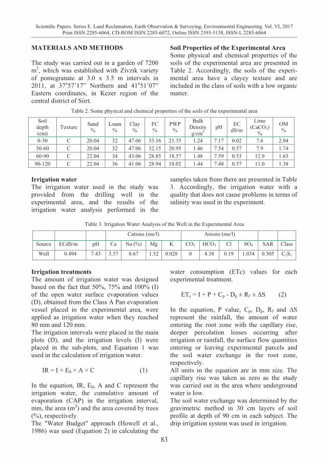
83
Scientific Papers. Series E. Land Reclamation, Earth Observation & Surveying, Environmental Engineering. Vol. VI, 2017Print ISSN 2285-6064, CD-ROM ISSN 2285-6072, Online ISSN 2393-5138, ISSN-L 2285-6064
pomegranate fruit consists of a large number of fruit seeds containing water, there is a high osmotic pressure at the time of water stress, and the grains get swollen because of receiving large amounts of water when it is irrigated im-mediately after it, and the internal pressure on the peel increases. Therefore, the fruit becomes susceptible to cracking. For that reason it is important that the irrigations are regular and programmed (Yılmaz and Özgüven, 2003). Coşkun (2006), who states that the sufficient soil moisture should be provided during the maturation period of the fruit, points out that the presence of the sufficient soil moisture especially in summer and at the beginning of autumn will also decrease the rate of fruit cracking. The region is usually under the influence of dry and hot air masses during summer. The daytime maximum temperature rises above 40oC. In addition, dry and hot winds called "simum" increase evaporation and also cause dust storms in this period. During the winter season, the region falls under the influence of rainy fronts until April. According to the results of the measurement performed in the
experimental area during the period 1960-2013, the annual average temperature value was determined to be 16.1ºC. The average temperature values falling to the lowest level in winter months tend to increase rapidly as of March and rise above 25ºC in May and June (Table 1). In the experimental area, it is seen that the average temperatures do not fall below 26ºC during the summer period (June, July, August) and below -2.7ºC during the winter period (December, January, February). As a consequence of the continental climate observed in the study, the temperature differ-rence between the seasons is quite high. While the average temperature of summer months in the central district of Siirt is 28.8˚C, the average temperature of winter months is 3.8˚C. The temperature values of the experimental area are higher compared to many regions of Turkey. There are some factors that affect this situation. One of them is the latitude, and the other one is continentally. As it is known, the weather becomes warmer rapidly and excessively in places where the continental climate is observed. Therefore, summer is very hot, and winter is cold.
Table 1. Some Meteorological Data of Experimental Area for Long Term Period (1960-2013)
Months
Janu
ary
Febr
uary
Mar
ch
Apr
il
May
June
July
Aug
ust
Sept
embe
r Nov
embe
r Oct
ober
Dec
embe
r
Ave
rage
Ave. Max. Temp. oC 6.7 8.8 13.8 19.3 25.3 32.3 37.2 37.0 32.4 24.7 15.4 8.7 21.8 Ave. Min. Temp. oC -0.5 0.6 4.5 9.3 13.7 19.2 23.5 23.2 18.9 12.9 6.3 1.6 11.1 Ave. Temp. oC -2.7 4.2 8.6 13.9 19.4 26.0 30.5 30.0 25.1 18.1 10.2 4.7 16.1 Min. Temp.oC -11 -9.5 -7.2 -3.8 2.0 5.4 13.7 19.7 8.5 3.8 -4.3 -11.7 -3.5 Max. Temp. oC 15.2 17.3 28.5 32.9 36.1 40.2 44 43.4 39.5 33.6 18.6 14.3 33.6 Ave. Wind Speed (m/s) 0.3 0.5 0.6 0.6 0.6 0.6 0.6 0.6 0.6 0.5 0.3 0.3 0.3 Max. Wind Speed (m/s) 4.2 3.4 2.4 2.6 2.6 4.2 3.8 4.7 4.7 5.8 5.2 2.4 4.2
Many important studies on pomegranate irrigation have been carried out until today. However, no study on Siirt region and Zivzikpomegranate, in particular, has been encountered. Such a study has been required to solve the problems arising from irrigation of Zivzik pomegranate, which has an economic value and is cultivated in the region. In this study, an attempt to achieve the most appropriate irrigation programs in Zivzik
pomegranate variety, which is widely cultivated and has an economic value in Siirt region, was made, and the tree fruit yield and plant-water relationships were examined. It was aimed to minimise the yield losses due to irrigation, which is one of the most important problems of pomegranate cultivation and is shown as the cause of fruit cracking, by applying the appropriate irrigation programs.
MATERIALS AND METHODS The study was carried out in a garden of 7200 m2, which was established with Zivzik variety of pomegranate at 3.0 x 3.5 m intervals in 2011, at 37o57’17” Northern and 41o51’07” Eastern coordinates, in Kezer region of the central district of Siirt.
Soil Properties of the Experimental Area Some physical and chemical properties of the soils of the experimental area are presented in Table 2. Accordingly, the soils of the experi-mental area have a clayey texture and are included in the class of soils with a low organic matter.
Table 2. Some physical and chemical properties of the soils of the experimental area
Soil depth (cm)
Texture Sand %
Loam %
Clay %
FC %
PWP %
Bulk Density g/cm3
pH EC dS/m
Lime (CaCO3)
%
OM %
0-30 C 20.04 32 47.06 33.16 21.35 1.24 7.17 0.02 7.6 2.04 30-60 C 20.04 32 47.06 32.15 20.95 1.46 7.54 0.57 7.9 1.74 60-90 C 22.04 34 43.06 28.85 18.57 1.48 7.59 0.53 12.9 1.63 90-120 C 22.04 36 41.06 28.94 18.02 1.44 7.48 0.57 11.0 1.38
Irrigation water The irrigation water used in the study was provided from the drilling well in the experimental area, and the results of the irrigation water analysis performed in the
samples taken from there are presented in Table 3. Accordingly, the irrigation water with a quality that does not cause problems in terms of salinity was used in the experiment.
Table 3. Irrigation Water Analysis of the Well in the Experimental Area
Cations (me/l) Anions (me/l)
Source ECdS/m pH Ca Na (%) Mg K CO3 HCO3 Cl SO4 SAR Class
Well 0.494 7.43 3.57 8.67 1.52 0.028 0 4.38 0.19 1.034 0.305 C2S1
Irrigation treatments The amount of irrigation water was designed based on the fact that 50%, 75% and 100% (I) of the open water surface evaporation values (D), obtained from the Class A Pan evaporation vessel placed in the experimental area, were applied as irrigation water when they reached 80 mm and 120 mm. The irrigation intervals were placed in the main plots (D), and the irrigation levels (I) were placed in the sub-plots, and Equation 1 was used in the calculation of irrigation water.
IR = I × E0 × A × C (1) In the equation, IR, E0, A and C represent the irrigation water, the cumulative amount of evaporation (CAP) in the irrigation interval, mm, the area (m2) and the area covered by trees (%), respectively. The "Water Budget" approach (Howell et al., 1986) was used (Equation 2) in calculating the
water consumption (ETc) values for each experimental treatment.
ETc = I + P + Cp - Dp ± Rf ± ΔS (2) In the equation, P value, Cp, Dp, Rf and ∆S represent the rainfall, the amount of water entering the root zone with the capillary rise, deeper percolation losses occurring after irrigation or rainfall, the surface flow quantities entering or leaving experimental parcels and the soil water exchange in the root zone, respectively. All units in the equation are in mm size. The capillary rise was taken as zero as the study was carried out in the area where underground water is low. The soil water exchange was determined by the gravimetric method in 30 cm layers of soil profile at depth of 90 cm in each subject. The drip irrigation system was used in irrigation.
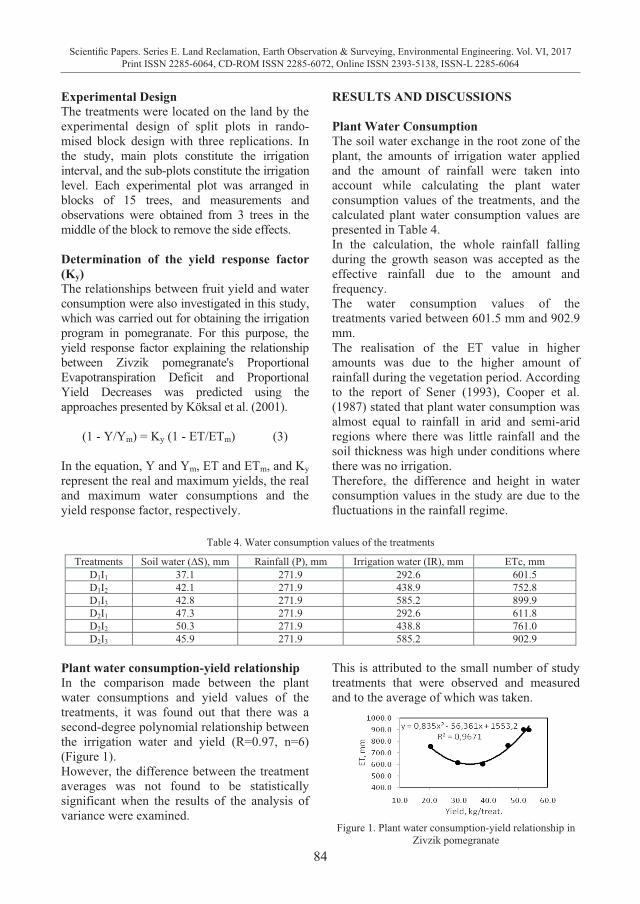
84
Scientific Papers. Series E. Land Reclamation, Earth Observation & Surveying, Environmental Engineering. Vol. VI, 2017Print ISSN 2285-6064, CD-ROM ISSN 2285-6072, Online ISSN 2393-5138, ISSN-L 2285-6064
Experimental Design The treatments were located on the land by the experimental design of split plots in rando-mised block design with three replications. In the study, main plots constitute the irrigation interval, and the sub-plots constitute the irrigation level. Each experimental plot was arranged in blocks of 15 trees, and measurements and observations were obtained from 3 trees in the middle of the block to remove the side effects. Determination of the yield response factor (Ky) The relationships between fruit yield and water consumption were also investigated in this study, which was carried out for obtaining the irrigation program in pomegranate. For this purpose, the yield response factor explaining the relationship between Zivzik pomegranate's Proportional Evapotranspiration Deficit and Proportional Yield Decreases was predicted using the approaches presented by Köksal et al. (2001).
(1 - Y/Ym) = Ky (1 - ET/ETm) (3) In the equation, Y and Ym, ET and ETm, and Ky represent the real and maximum yields, the real and maximum water consumptions and the yield response factor, respectively.
RESULTS AND DISCUSSIONS Plant Water Consumption The soil water exchange in the root zone of the plant, the amounts of irrigation water applied and the amount of rainfall were taken into account while calculating the plant water consumption values of the treatments, and the calculated plant water consumption values are presented in Table 4. In the calculation, the whole rainfall falling during the growth season was accepted as the effective rainfall due to the amount and frequency. The water consumption values of the treatments varied between 601.5 mm and 902.9 mm. The realisation of the ET value in higher amounts was due to the higher amount of rainfall during the vegetation period. According to the report of Sener (1993), Cooper et al. (1987) stated that plant water consumption was almost equal to rainfall in arid and semi-arid regions where there was little rainfall and the soil thickness was high under conditions where there was no irrigation. Therefore, the difference and height in water consumption values in the study are due to the fluctuations in the rainfall regime.
Table 4. Water consumption values of the treatments
Treatments Soil water (∆S), mm Rainfall (P), mm Irrigation water (IR), mm ETc, mm D1I1 37.1 271.9 292.6 601.5 D1I2 42.1 271.9 438.9 752.8 D1I3 42.8 271.9 585.2 899.9 D2I1 47.3 271.9 292.6 611.8 D2I2 50.3 271.9 438.8 761.0 D2I3 45.9 271.9 585.2 902.9
Plant water consumption-yield relationship In the comparison made between the plant water consumptions and yield values of the treatments, it was found out that there was a second-degree polynomial relationship between the irrigation water and yield (R=0.97, n=6) (Figure 1). However, the difference between the treatment averages was not found to be statistically significant when the results of the analysis of variance were examined.
This is attributed to the small number of study treatments that were observed and measured and to the average of which was taken.
Figure 1. Plant water consumption-yield relationship in
Zivzik pomegranate
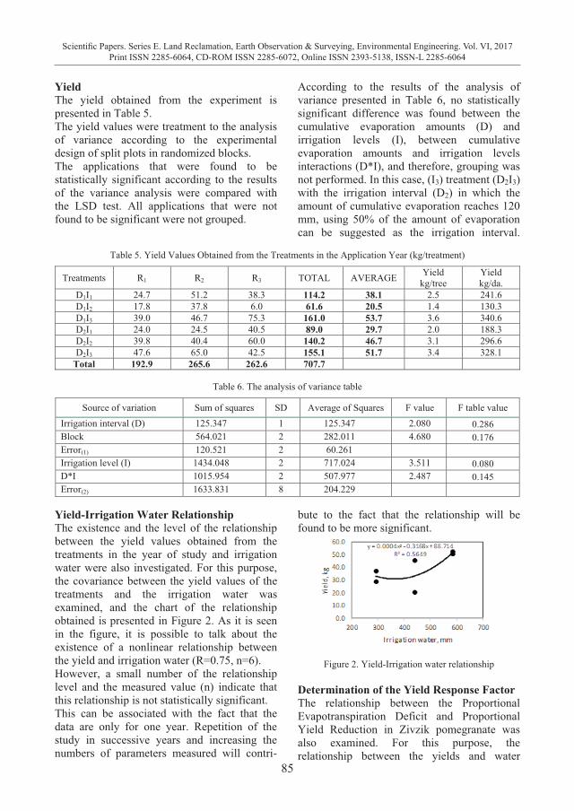
85
Scientific Papers. Series E. Land Reclamation, Earth Observation & Surveying, Environmental Engineering. Vol. VI, 2017Print ISSN 2285-6064, CD-ROM ISSN 2285-6072, Online ISSN 2393-5138, ISSN-L 2285-6064
Experimental Design The treatments were located on the land by the experimental design of split plots in rando-mised block design with three replications. In the study, main plots constitute the irrigation interval, and the sub-plots constitute the irrigation level. Each experimental plot was arranged in blocks of 15 trees, and measurements and observations were obtained from 3 trees in the middle of the block to remove the side effects. Determination of the yield response factor (Ky) The relationships between fruit yield and water consumption were also investigated in this study, which was carried out for obtaining the irrigation program in pomegranate. For this purpose, the yield response factor explaining the relationship between Zivzik pomegranate's Proportional Evapotranspiration Deficit and Proportional Yield Decreases was predicted using the approaches presented by Köksal et al. (2001).
(1 - Y/Ym) = Ky (1 - ET/ETm) (3) In the equation, Y and Ym, ET and ETm, and Ky represent the real and maximum yields, the real and maximum water consumptions and the yield response factor, respectively.
RESULTS AND DISCUSSIONS Plant Water Consumption The soil water exchange in the root zone of the plant, the amounts of irrigation water applied and the amount of rainfall were taken into account while calculating the plant water consumption values of the treatments, and the calculated plant water consumption values are presented in Table 4. In the calculation, the whole rainfall falling during the growth season was accepted as the effective rainfall due to the amount and frequency. The water consumption values of the treatments varied between 601.5 mm and 902.9 mm. The realisation of the ET value in higher amounts was due to the higher amount of rainfall during the vegetation period. According to the report of Sener (1993), Cooper et al. (1987) stated that plant water consumption was almost equal to rainfall in arid and semi-arid regions where there was little rainfall and the soil thickness was high under conditions where there was no irrigation. Therefore, the difference and height in water consumption values in the study are due to the fluctuations in the rainfall regime.
Table 4. Water consumption values of the treatments
Treatments Soil water (∆S), mm Rainfall (P), mm Irrigation water (IR), mm ETc, mm D1I1 37.1 271.9 292.6 601.5 D1I2 42.1 271.9 438.9 752.8 D1I3 42.8 271.9 585.2 899.9 D2I1 47.3 271.9 292.6 611.8 D2I2 50.3 271.9 438.8 761.0 D2I3 45.9 271.9 585.2 902.9
Plant water consumption-yield relationship In the comparison made between the plant water consumptions and yield values of the treatments, it was found out that there was a second-degree polynomial relationship between the irrigation water and yield (R=0.97, n=6) (Figure 1). However, the difference between the treatment averages was not found to be statistically significant when the results of the analysis of variance were examined.
This is attributed to the small number of study treatments that were observed and measured and to the average of which was taken.
Figure 1. Plant water consumption-yield relationship in
Zivzik pomegranate
Yield The yield obtained from the experiment is presented in Table 5. The yield values were treatment to the analysis of variance according to the experimental design of split plots in randomized blocks. The applications that were found to be statistically significant according to the results of the variance analysis were compared with the LSD test. All applications that were not found to be significant were not grouped.
According to the results of the analysis of variance presented in Table 6, no statistically significant difference was found between the cumulative evaporation amounts (D) and irrigation levels (I), between cumulative evaporation amounts and irrigation levels interactions (D*I), and therefore, grouping was not performed. In this case, (I3) treatment (D2I3) with the irrigation interval (D2) in which the amount of cumulative evaporation reaches 120 mm, using 50% of the amount of evaporation can be suggested as the irrigation interval.
Table 5. Yield Values Obtained from the Treatments in the Application Year (kg/treatment)
Treatments R1 R2 R3 TOTAL AVERAGE Yield kg/tree
Yield kg/da.
D1I1 24.7 51.2 38.3 114.2 38.1 2.5 241.6 D1I2 17.8 37.8 6.0 61.6 20.5 1.4 130.3 D1I3 39.0 46.7 75.3 161.0 53.7 3.6 340.6 D2I1 24.0 24.5 40.5 89.0 29.7 2.0 188.3 D2I2 39.8 40.4 60.0 140.2 46.7 3.1 296.6 D2I3 47.6 65.0 42.5 155.1 51.7 3.4 328.1
Total 192.9 265.6 262.6 707.7
Table 6. The analysis of variance table
Source of variation Sum of squares SD Average of Squares F value F table value Irrigation interval (D) 125.347 1 125.347 2.080 0.286 Block 564.021 2 282.011 4.680 0.176 Error(1) 120.521 2 60.261 Irrigation level (I) 1434.048 2 717.024 3.511 0.080 D*I 1015.954 2 507.977 2.487 0.145 Error(2) 1633.831 8 204.229
Yield-Irrigation Water Relationship The existence and the level of the relationship between the yield values obtained from the treatments in the year of study and irrigation water were also investigated. For this purpose, the covariance between the yield values of the treatments and the irrigation water was examined, and the chart of the relationship obtained is presented in Figure 2. As it is seen in the figure, it is possible to talk about the existence of a nonlinear relationship between the yield and irrigation water (R=0.75, n=6). However, a small number of the relationship level and the measured value (n) indicate that this relationship is not statistically significant. This can be associated with the fact that the data are only for one year. Repetition of the study in successive years and increasing the numbers of parameters measured will contri-
bute to the fact that the relationship will be found to be more significant.
Figure 2. Yield-Irrigation water relationship
Determination of the Yield Response Factor The relationship between the Proportional Evapotranspiration Deficit and Proportional Yield Reduction in Zivzik pomegranate was also examined. For this purpose, the relationship between the yields and water
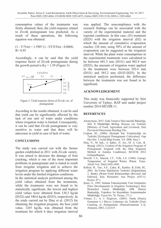
86
Scientific Papers. Series E. Land Reclamation, Earth Observation & Surveying, Environmental Engineering. Vol. VI, 2017Print ISSN 2285-6064, CD-ROM ISSN 2285-6072, Online ISSN 2393-5138, ISSN-L 2285-6064
consumption values of the treatments was firstly obtained; then, the yield response related to Zivzik pomegranate was predicted. As a result of these operations, the following equation was obtained. (1 - Y/Ym) = 1.5907 (1 - ET/ETm) - 0.0068; R= 0.95 Accordingly, it can be said that the yield response factor of Zivzik pomegranate during the growth period is Ky = 1.59 (Figure 3).
Ky = 1.59
R = 0.
00.20.40.60.8
00.10.20.30.4
1-Ya
/Ym
1-ETa/ETm
Figure 3. Yield response factor of Zivzik var. of
pomegranate According to the results obtained, it can be said that yield can be significantly affected by the lack of one unit of water under conditions where irrigation water is limited. Consequently, it can be said that Zivzik pomegranate is very sensitive to water and that there will be adecrease in yield in case of lack of water. CONCLUSIONS The study was carried out with the farmer garden established in 2011 with Zivzik variety. It was aimed to decrease the damage of fruit cracking, which is one of the most important problems in pomegranate and is stated to result from irregular irrigation and to achieve the irrigation program by applying different water levels under the limited irrigation conditions. In the statistical analysis performed among the yield values obtained from the treatments, while the treatments were not found to be statistically significant, the lowest and highest yield values were obtained from 130.3 kg/da (D1I2) and 340.6 kg/da (D1I3), respectively. In the study carried out by Dinç et al. (2012) for obtaining the irrigation program, the best yield value, 1265 kg/da, was obtained from the treatment for which 6 days irrigation interval
was applied. The noncompliance with the research findings can be associated with the variety of the experimental material and the regional conditions. In this case, (I3) treatment (D2I3) with the irrigation interval (D2) in which the amount of cumulative evaporation reaches 120 mm, using 50% of the amount of evaporation can be suggested as the irrigation interval. While the plant water consumptions in the experimental treatments were calculated to be between 601.5 mm (D1I1) and 902.9 mm (D2I3), the amounts of irrigation water applied to the treatments were between 292.6 mm (D1I1) and 585.2 mm (D1I3-D2I3). In the statistical analysis performed, the difference between the treatments was not found to be significant. ACKNOWLEDGEMENT This study was financially supported by Siirt University of Turkey, BAP unit under project number 2014-SİÜZİR-11. REFERENCES Anonymous, 2013. Gıda Tarımve Hayvancılık Bakanlığı,
Siirt İl Müdürlüğü Brifing Dosyası (in Turkish) [Ministry of Food, Agriculture and Livestock, Siirt Provincial Directorate Briefing File.
Coşkun, M., (2006). Ekolojik Nar Yetiştiriciliği (in Turkish) [Ecological Pomegranate Cultivation]. Gap Eko Der. 3 Aylık Bilgi Formu. Yıl: 2006, Sayı:1.
Dinç, N., M. Işık., A. Şahin., N. Arı., M. A. Can., R. Baştuğ. (2012). Creation of the Irrigation Program of Pomegranate Irrigated with the Drip Irrigation Method in Antalya Conditions]. BATEM 2012 GelişmeRaporu.
Howell, T.A., Musıck, J.T., Tolk, J.A. (1986). Canopy Temperature of Irrigated Winter Wheat. Trans. ASAE Vol. 29(6):1692-1699.
Köksal, H., Tarı, A.F., Çakır, R., Kanber, R.,Ünlü, M., 2001. Su-Verim İlişkileri(in Turkish) (Değiştirilmiş 2. Baskı) [Water-Yield Relationships (Revised 2nd Edition)]. Köy Hizmetleri Ana Projesi (435-1). Konya. 87 s.
Şener, S., 1993. Sulama Teknolojisinde Yeni Gelişmeler [New Developments in Irrigation Technology]. Köy Hizmetleri Genel Müdürlüğü, APK Dairesi Başkanlığı, Toprakve Su Kaynakları Araştırmaşube Müdürlüğü. Yayın No: 76, Tarsus, 171 s.
Yılmaz, C., A. I. Özgüven., (2003). Narda (Punica Granatum L.) Meyve Çatlaması (in Turkish) [Fruit Cracking in Pomegranate (PunicaGranatum L.)]. Alatarım, 2003, 2 (2):4-9.
87
Scientific Papers. Series E. Land Reclamation, Earth Observation & Surveying, Environmental Engineering. Vol. VI, 2017Print ISSN 2285-6064, CD-ROM ISSN 2285-6072, Online ISSN 2393-5138, ISSN-L 2285-6064
consumption values of the treatments was firstly obtained; then, the yield response related to Zivzik pomegranate was predicted. As a result of these operations, the following equation was obtained. (1 - Y/Ym) = 1.5907 (1 - ET/ETm) - 0.0068; R= 0.95 Accordingly, it can be said that the yield response factor of Zivzik pomegranate during the growth period is Ky = 1.59 (Figure 3).
Ky = 1.59
R = 0.
00.20.40.60.8
00.10.20.30.4
1-Ya
/Ym
1-ETa/ETm
Figure 3. Yield response factor of Zivzik var. of
pomegranate According to the results obtained, it can be said that yield can be significantly affected by the lack of one unit of water under conditions where irrigation water is limited. Consequently, it can be said that Zivzik pomegranate is very sensitive to water and that there will be adecrease in yield in case of lack of water. CONCLUSIONS The study was carried out with the farmer garden established in 2011 with Zivzik variety. It was aimed to decrease the damage of fruit cracking, which is one of the most important problems in pomegranate and is stated to result from irregular irrigation and to achieve the irrigation program by applying different water levels under the limited irrigation conditions. In the statistical analysis performed among the yield values obtained from the treatments, while the treatments were not found to be statistically significant, the lowest and highest yield values were obtained from 130.3 kg/da (D1I2) and 340.6 kg/da (D1I3), respectively. In the study carried out by Dinç et al. (2012) for obtaining the irrigation program, the best yield value, 1265 kg/da, was obtained from the treatment for which 6 days irrigation interval
was applied. The noncompliance with the research findings can be associated with the variety of the experimental material and the regional conditions. In this case, (I3) treatment (D2I3) with the irrigation interval (D2) in which the amount of cumulative evaporation reaches 120 mm, using 50% of the amount of evaporation can be suggested as the irrigation interval. While the plant water consumptions in the experimental treatments were calculated to be between 601.5 mm (D1I1) and 902.9 mm (D2I3), the amounts of irrigation water applied to the treatments were between 292.6 mm (D1I1) and 585.2 mm (D1I3-D2I3). In the statistical analysis performed, the difference between the treatments was not found to be significant. ACKNOWLEDGEMENT This study was financially supported by Siirt University of Turkey, BAP unit under project number 2014-SİÜZİR-11. REFERENCES Anonymous, 2013. Gıda Tarımve Hayvancılık Bakanlığı,
Siirt İl Müdürlüğü Brifing Dosyası (in Turkish) [Ministry of Food, Agriculture and Livestock, Siirt Provincial Directorate Briefing File.
Coşkun, M., (2006). Ekolojik Nar Yetiştiriciliği (in Turkish) [Ecological Pomegranate Cultivation]. Gap Eko Der. 3 Aylık Bilgi Formu. Yıl: 2006, Sayı:1.
Dinç, N., M. Işık., A. Şahin., N. Arı., M. A. Can., R. Baştuğ. (2012). Creation of the Irrigation Program of Pomegranate Irrigated with the Drip Irrigation Method in Antalya Conditions]. BATEM 2012 GelişmeRaporu.
Howell, T.A., Musıck, J.T., Tolk, J.A. (1986). Canopy Temperature of Irrigated Winter Wheat. Trans. ASAE Vol. 29(6):1692-1699.
Köksal, H., Tarı, A.F., Çakır, R., Kanber, R.,Ünlü, M., 2001. Su-Verim İlişkileri(in Turkish) (Değiştirilmiş 2. Baskı) [Water-Yield Relationships (Revised 2nd Edition)]. Köy Hizmetleri Ana Projesi (435-1). Konya. 87 s.
Şener, S., 1993. Sulama Teknolojisinde Yeni Gelişmeler [New Developments in Irrigation Technology]. Köy Hizmetleri Genel Müdürlüğü, APK Dairesi Başkanlığı, Toprakve Su Kaynakları Araştırmaşube Müdürlüğü. Yayın No: 76, Tarsus, 171 s.
Yılmaz, C., A. I. Özgüven., (2003). Narda (Punica Granatum L.) Meyve Çatlaması (in Turkish) [Fruit Cracking in Pomegranate (PunicaGranatum L.)]. Alatarım, 2003, 2 (2):4-9.
BENCHMARKING PERFORMANCE OF LARGE SCALE IRRIGATION
SCHEMES WITH COMPARATIVE INDICATORS IN TURKEY
Hasan DEĞİRMENCİ, Çağatay TANRIVERDİ, Fırat ARSLAN, Engin GÖNEN
Kahramanmaras Sutcu Imam University of Biosystem Engineering, 46100 Kahramanmaras, Turkey
Corresponding author email: [email protected]
Abstract Irrigation management is one of the key factors for the sustainability of irrigated agriculture. There has been a good number of performance indicators developed for the assessment of irrigation schemes. DSI (State Hydraulic Works) datas for 5 years (2011-2014) were used to calculate indicators of irrigated agricultural output. The most important one among them is the four basic comparative performance indicators related output to unit land and water. These “external” indicators provide the basis for comparison of irrigated agriculture performance. Comparative indicators are the output per cropped area ($/ha), output per unit command ($/ha), output per unit irrigation supply ($/m3), and output per unit water consumed ($/m3). In this paper, obtained the data that regarding irrigated cropped area, production, which are the output of the irrigated area in terms of gross or net value of production measured at local prices, command area, diverted irrigation supply, volume of water consumed by ET. This data were used to calculate comparative indicators. This study, in three climatic zones (Continental, Mediterranean and Black Sea) fourteen irrigation schemes, more than 20.000 ha of command area for each scheme, were assessed. Irrigation schemes were classified with regard to crop pattern. As a result of the study, based on the 2011-2014 years output per unit command area, output per cropped irrigated area, output per unit irrigation supply, output per unit water consumed were determined as 1040-7669 US$/ha, 2387-10129 US$/ha, 0.13-1.38 US$/m3, and 0.60-2.29 US$/m3, respectively. Calculated comparative indicators compared with each irrigation scheme's crop pattern and climatic zone. In addition, results compared with irrigation schemes in similar climatic zone with similar crop pattern. In conclusion, it was determined that crop pattern is the most effective factor to success of irrigation schemes. Key words: comparative indicators, cropping pattern, irrigation scheme, irrigated area, production INTRODUCTION Agriculture is the major source of livelihood and employment in developing and underde-veloped countries. 70% of the water used in the world is used in the irrigation. Irrigated agriculture has vital importance in underde-veloped countries. The use of technology in the transmission and distribution of irrigation water in underdeveloped countries is very low. The main problems are the irrigation ratio and the low irrigation efficiency. Irrigation ratio of irrigation schemes in Turkey is 62%. The irrigation schemes in Turkey have low irrigation efficiency. The total surface area of Turkey is 78 million hectares (783.577 km2), 28 million hectares of which are cultivable agricultural lands. In 2014, a total of .6.09 million hectares of land has been put into operation in Turkey. Of the irrigation areas put into operation, approxi-mately 81% of them are irrigated by surface
water resources, while the remaining 19% of them by underground water resources. In Turkey, the management of irrigation schemes has been assigned to the water user organi-zations since 1994. According to this irrigation management assignment scheme, the irrigation areas that were previously run by the state have been assigned to the irrigation associations (89.1%), cooperatives (5.1%), municipalities (3%), legal village entities (1.6%) and the unions of village delivery service (0.9%) (DSI, 2015). Four basic benchmarking indicators developed by Molden et al. (1998) are used in this study. These indicators are related cropped area, command area, irrigation supply, water consumed and evapotranspiration. Various studies are conducted in the World and Turkey (Kukul et al., 2008; Cakmak et al., 2010; Uysal and Atis, 2010). Senerve Albut (2011) used comparative indicators in 10 irrigation schemes in Trakya region in Turkey. In this study output per unit command area, output per cropped
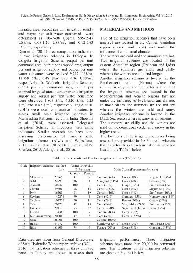
88
Scientific Papers. Series E. Land Reclamation, Earth Observation & Surveying, Environmental Engineering. Vol. VI, 2017Print ISSN 2285-6064, CD-ROM ISSN 2285-6072, Online ISSN 2393-5138, ISSN-L 2285-6064
irrigated area, output per unit irrigation supply and output per unit water consumed were determined as 106-7498 US$/ha, 999-3947 US$/ha, 0.06-1.29 US$/m3, and 0.12-0.63 US$/m3, respectively. Djen et al. (2011) used comparative indicators in two irrigation schemes in Ethiopia. In Golgota Irrigation Scheme, output per unit command area, output per cropped area, output per unit irrigation supply and output per unit water consumed were realized 9.212 US$/ha, 12.999 $/ha, 0.48 $/m3 and 0.86 US$/m3, respectively. In Wedecha Irrigation Scheme, output per unit command area, output per cropped irrigated area, output per unit irrigation supply and output per unit water consumed were observed 1.808 $/ha, 4.520 $/ha, 0.25 $/m3 and 0.49 $/m3, respectively. Ingle et al. (2015) were used comparative indicators to assess small scale irrigation schemes in Maharashtra Ratnagiri region in India. Shrestha et al. (2014), were assessed Telegasari Irrigation Scheme in Indonesia with same indicators. Similar research has been done assessing performance of various scale irrigation schemes (Alwis and Wijesekara, 2011; Lakmali et al., 2015; Bareng et al., 2015; Shenkut, 2015; Adongo et al., 2016).
MATERIALS AND METHODS Two of the irrigation schemes that have been assessed are located in the Central Anatolian region (Çumra and İvriz) and under the influence of continental climate. The winters are cold and the summers are hot. Two irrigation schemes are located in the eastern Anatolian region (Erzincan and Iğdır) where the summers are short and chilly whereas the winters are cold and longer. Another irrigation scheme is located in the Southeastern region (Harran) where the summer is very hot and the winter is mild. 5 of the irrigation schemes are located in the Mediterranean and Aegean regions that are under the influence of Mediterranean climate. In those places, the summers are hot and dry whereas the winters are mild and rainy. Another irrigation scheme is located in the Black Sea region where is rainy in all seasons. The summers are chilly and the winters are mild on the coasts, but colder and snowy in the higher areas. The locations of the irrigation schemes being assessed are provided in the Figure 1, whereas the characteristics of each irrigation scheme are listed in the Table 1 below.
Table 1. Characteristics of Fourteen irrigation schemes (DSİ, 2016)
Data used are taken from General Directorate of State Hydraulic Works report archive (DSİ, 2016). 14 irrigation schemes in three climatic zones in Turkey are chosen to assess their
irrigation performance. These irrigation schemes have more than 20,000 ha command area. The locations of the irrigation schemes are given on Figure 1 below.
Code Irrigation Scheme Surface (ha)
Water Diversion (% by area)
Main Crops (Percentages by area)
Gravity Pumped 1 Menemen 22865 91 9 Cotton (56%) Corn (18%) Vegetables (8%) 2 Salihli 22797 96 4 Vineyard (44%) Corn (32%) Cereals (9%) 3 Ahmetli 50232 100 - Corn (53%) Grape (35%) Fruit trees (4%) 4 Çumra 59560 88 12 Cereals (53%) Corn (35%) Sugarbeet (12%) 5 İvriz 36108 81 19 Cereals (46%) Corn (31%) Sunflower (10%) 6 Seyhan 142274 99 1 Corn (42%) Citruses (15%) Nursery tree (11%) 7 Ceyhan 101726 89 11 Corn (79%) Peanut (10%) Cotton (56%) 8 Tokat 20275 82 18 Corn (24%) Vegetables (20%) Fruit trees (15%) 9 Erzincan 29112 63 37 Cereals (50%) Sugar beet (16%) Bean (15%)
10 Harran 134366 100 - Cotton (78%) Cereals (22) - 11 Kahramanmaraş 20000 97 3 Corn (60%) Cereals (32%) - 12 Söke 26000 100 - Cotton (100%) - - 13 Baklan 44072 100 - Sunflower (54%) Corn (15%) Fruit trees (10%) 14 Iğdır 61900 94 6 Forage (50%) Corn (31%) Grassland (13%)
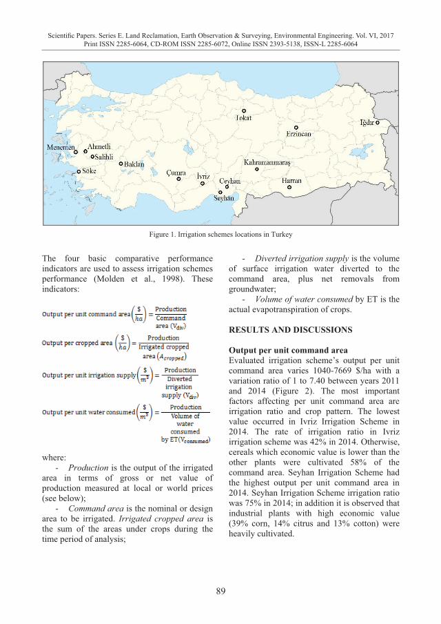
89
Scientific Papers. Series E. Land Reclamation, Earth Observation & Surveying, Environmental Engineering. Vol. VI, 2017Print ISSN 2285-6064, CD-ROM ISSN 2285-6072, Online ISSN 2393-5138, ISSN-L 2285-6064
irrigated area, output per unit irrigation supply and output per unit water consumed were determined as 106-7498 US$/ha, 999-3947 US$/ha, 0.06-1.29 US$/m3, and 0.12-0.63 US$/m3, respectively. Djen et al. (2011) used comparative indicators in two irrigation schemes in Ethiopia. In Golgota Irrigation Scheme, output per unit command area, output per cropped area, output per unit irrigation supply and output per unit water consumed were realized 9.212 US$/ha, 12.999 $/ha, 0.48 $/m3 and 0.86 US$/m3, respectively. In Wedecha Irrigation Scheme, output per unit command area, output per cropped irrigated area, output per unit irrigation supply and output per unit water consumed were observed 1.808 $/ha, 4.520 $/ha, 0.25 $/m3 and 0.49 $/m3, respectively. Ingle et al. (2015) were used comparative indicators to assess small scale irrigation schemes in Maharashtra Ratnagiri region in India. Shrestha et al. (2014), were assessed Telegasari Irrigation Scheme in Indonesia with same indicators. Similar research has been done assessing performance of various scale irrigation schemes (Alwis and Wijesekara, 2011; Lakmali et al., 2015; Bareng et al., 2015; Shenkut, 2015; Adongo et al., 2016).
MATERIALS AND METHODS Two of the irrigation schemes that have been assessed are located in the Central Anatolian region (Çumra and İvriz) and under the influence of continental climate. The winters are cold and the summers are hot. Two irrigation schemes are located in the eastern Anatolian region (Erzincan and Iğdır) where the summers are short and chilly whereas the winters are cold and longer. Another irrigation scheme is located in the Southeastern region (Harran) where the summer is very hot and the winter is mild. 5 of the irrigation schemes are located in the Mediterranean and Aegean regions that are under the influence of Mediterranean climate. In those places, the summers are hot and dry whereas the winters are mild and rainy. Another irrigation scheme is located in the Black Sea region where is rainy in all seasons. The summers are chilly and the winters are mild on the coasts, but colder and snowy in the higher areas. The locations of the irrigation schemes being assessed are provided in the Figure 1, whereas the characteristics of each irrigation scheme are listed in the Table 1 below.
Table 1. Characteristics of Fourteen irrigation schemes (DSİ, 2016)
Data used are taken from General Directorate of State Hydraulic Works report archive (DSİ, 2016). 14 irrigation schemes in three climatic zones in Turkey are chosen to assess their
irrigation performance. These irrigation schemes have more than 20,000 ha command area. The locations of the irrigation schemes are given on Figure 1 below.
Code Irrigation Scheme Surface (ha)
Water Diversion (% by area)
Main Crops (Percentages by area)
Gravity Pumped 1 Menemen 22865 91 9 Cotton (56%) Corn (18%) Vegetables (8%) 2 Salihli 22797 96 4 Vineyard (44%) Corn (32%) Cereals (9%) 3 Ahmetli 50232 100 - Corn (53%) Grape (35%) Fruit trees (4%) 4 Çumra 59560 88 12 Cereals (53%) Corn (35%) Sugarbeet (12%) 5 İvriz 36108 81 19 Cereals (46%) Corn (31%) Sunflower (10%) 6 Seyhan 142274 99 1 Corn (42%) Citruses (15%) Nursery tree (11%) 7 Ceyhan 101726 89 11 Corn (79%) Peanut (10%) Cotton (56%) 8 Tokat 20275 82 18 Corn (24%) Vegetables (20%) Fruit trees (15%) 9 Erzincan 29112 63 37 Cereals (50%) Sugar beet (16%) Bean (15%)
10 Harran 134366 100 - Cotton (78%) Cereals (22) - 11 Kahramanmaraş 20000 97 3 Corn (60%) Cereals (32%) - 12 Söke 26000 100 - Cotton (100%) - - 13 Baklan 44072 100 - Sunflower (54%) Corn (15%) Fruit trees (10%) 14 Iğdır 61900 94 6 Forage (50%) Corn (31%) Grassland (13%)
Figure 1. Irrigation schemes locations in Turkey
The four basic comparative performance indicators are used to assess irrigation schemes performance (Molden et al., 1998). These indicators:
where: - Production is the output of the irrigated
area in terms of gross or net value of production measured at local or world prices (see below);
- Command area is the nominal or design area to be irrigated. Irrigated cropped area is the sum of the areas under crops during the time period of analysis;
- Diverted irrigation supply is the volume of surface irrigation water diverted to the command area, plus net removals from groundwater;
- Volume of water consumed by ET is the actual evapotranspiration of crops. RESULTS AND DISCUSSIONS Output per unit command area Evaluated irrigation scheme’s output per unit command area varies 1040-7669 $/ha with a variation ratio of 1 to 7.40 between years 2011 and 2014 (Figure 2). The most important factors affecting per unit command area are irrigation ratio and crop pattern. The lowest value occurred in Ivriz Irrigation Scheme in 2014. The rate of irrigation ratio in Ivriz irrigation scheme was 42% in 2014. Otherwise, cereals which economic value is lower than the other plants were cultivated 58% of the command area. Seyhan Irrigation Scheme had the highest output per unit command area in 2014. Seyhan Irrigation Scheme irrigation ratio was 75% in 2014; in addition it is observed that industrial plants with high economic value (39% corn, 14% citrus and 13% cotton) were heavily cultivated.
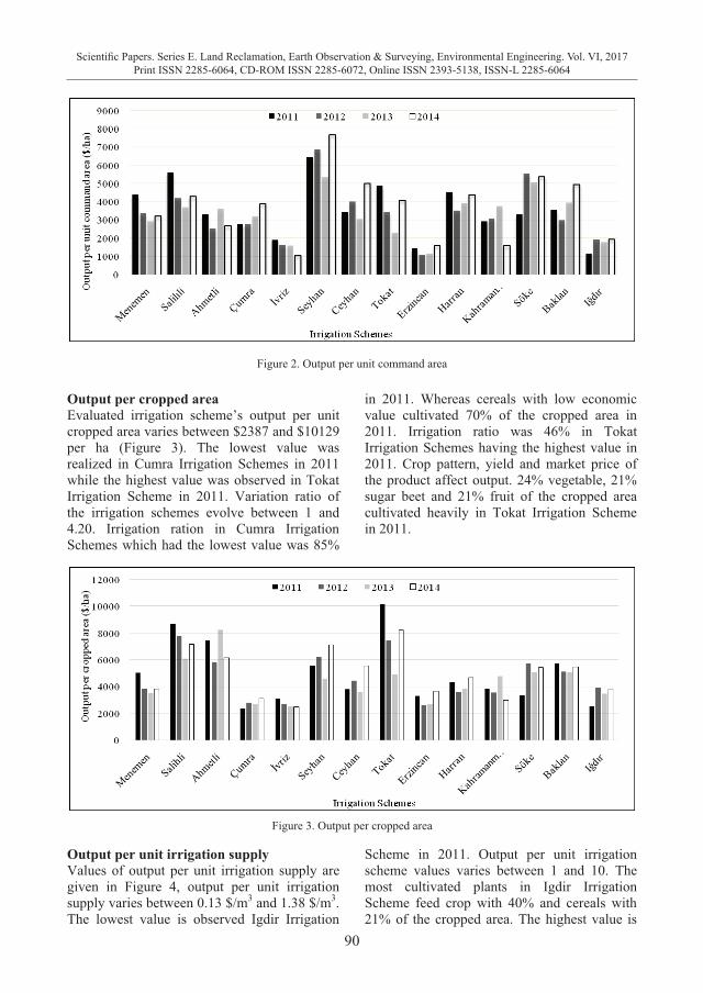
90
Scientific Papers. Series E. Land Reclamation, Earth Observation & Surveying, Environmental Engineering. Vol. VI, 2017Print ISSN 2285-6064, CD-ROM ISSN 2285-6072, Online ISSN 2393-5138, ISSN-L 2285-6064
Figure 2. Output per unit command area
Output per cropped area Evaluated irrigation scheme’s output per unit cropped area varies between $2387 and $10129 per ha (Figure 3). The lowest value was realized in Cumra Irrigation Schemes in 2011 while the highest value was observed in Tokat Irrigation Scheme in 2011. Variation ratio of the irrigation schemes evolve between 1 and 4.20. Irrigation ration in Cumra Irrigation Schemes which had the lowest value was 85%
in 2011. Whereas cereals with low economic value cultivated 70% of the cropped area in 2011. Irrigation ratio was 46% in Tokat Irrigation Schemes having the highest value in 2011. Crop pattern, yield and market price of the product affect output. 24% vegetable, 21% sugar beet and 21% fruit of the cropped area cultivated heavily in Tokat Irrigation Scheme in 2011.
Figure 3. Output per cropped area
Output per unit irrigation supply Values of output per unit irrigation supply are given in Figure 4, output per unit irrigation supply varies between 0.13 $/m3 and 1.38 $/m3. The lowest value is observed Igdir Irrigation
Scheme in 2011. Output per unit irrigation scheme values varies between 1 and 10. The most cultivated plants in Igdir Irrigation Scheme feed crop with 40% and cereals with 21% of the cropped area. The highest value is
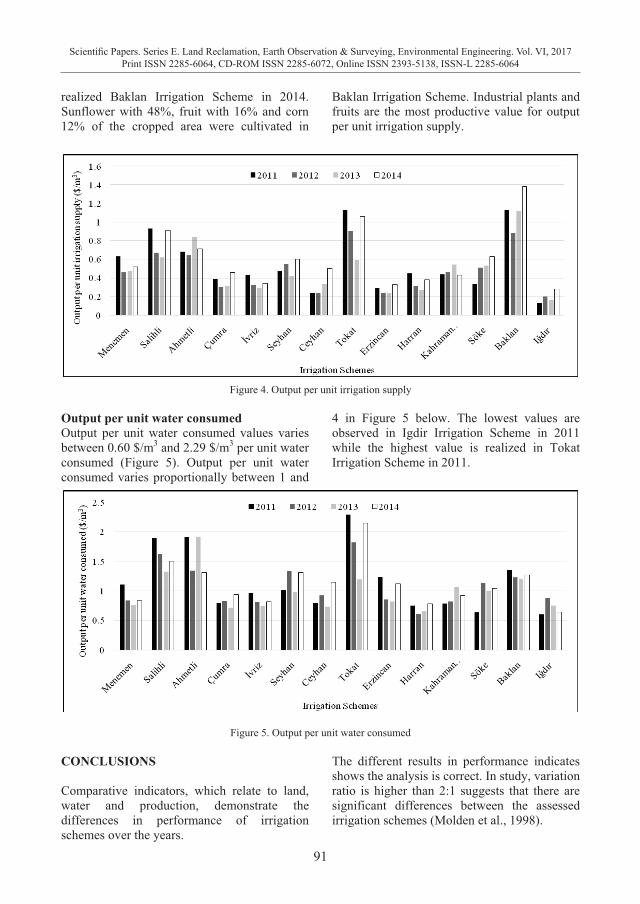
91
Scientific Papers. Series E. Land Reclamation, Earth Observation & Surveying, Environmental Engineering. Vol. VI, 2017Print ISSN 2285-6064, CD-ROM ISSN 2285-6072, Online ISSN 2393-5138, ISSN-L 2285-6064
Figure 2. Output per unit command area
Output per cropped area Evaluated irrigation scheme’s output per unit cropped area varies between $2387 and $10129 per ha (Figure 3). The lowest value was realized in Cumra Irrigation Schemes in 2011 while the highest value was observed in Tokat Irrigation Scheme in 2011. Variation ratio of the irrigation schemes evolve between 1 and 4.20. Irrigation ration in Cumra Irrigation Schemes which had the lowest value was 85%
in 2011. Whereas cereals with low economic value cultivated 70% of the cropped area in 2011. Irrigation ratio was 46% in Tokat Irrigation Schemes having the highest value in 2011. Crop pattern, yield and market price of the product affect output. 24% vegetable, 21% sugar beet and 21% fruit of the cropped area cultivated heavily in Tokat Irrigation Scheme in 2011.
Figure 3. Output per cropped area
Output per unit irrigation supply Values of output per unit irrigation supply are given in Figure 4, output per unit irrigation supply varies between 0.13 $/m3 and 1.38 $/m3. The lowest value is observed Igdir Irrigation
Scheme in 2011. Output per unit irrigation scheme values varies between 1 and 10. The most cultivated plants in Igdir Irrigation Scheme feed crop with 40% and cereals with 21% of the cropped area. The highest value is
realized Baklan Irrigation Scheme in 2014. Sunflower with 48%, fruit with 16% and corn 12% of the cropped area were cultivated in
Baklan Irrigation Scheme. Industrial plants and fruits are the most productive value for output per unit irrigation supply.
Figure 4. Output per unit irrigation supply
Output per unit water consumed Output per unit water consumed values varies between 0.60 $/m3 and 2.29 $/m3 per unit water consumed (Figure 5). Output per unit water consumed varies proportionally between 1 and
4 in Figure 5 below. The lowest values are observed in Igdir Irrigation Scheme in 2011 while the highest value is realized in Tokat Irrigation Scheme in 2011.
Figure 5. Output per unit water consumed CONCLUSIONS Comparative indicators, which relate to land, water and production, demonstrate the differences in performance of irrigation schemes over the years.
The different results in performance indicates shows the analysis is correct. In study, variation ratio is higher than 2:1 suggests that there are significant differences between the assessed irrigation schemes (Molden et al., 1998).
92
Scientific Papers. Series E. Land Reclamation, Earth Observation & Surveying, Environmental Engineering. Vol. VI, 2017Print ISSN 2285-6064, CD-ROM ISSN 2285-6072, Online ISSN 2393-5138, ISSN-L 2285-6064
Performance differences between irrigation networks depend on the management scheme, infrastructure, water distribution and distribution planning, climatic conditions of the region and socio-economic conditions of farmers. Assessment of irrigation schemes with comparative indicators is important appliance to decision makers. It is also useful in responding to the question "Do I do the right thing?" for irrigation managers (Murray-Rust and Snellen, 1993). Performance indicators can be used to identify long-term plans, to identify and confirm long-term strategic goals. As a result of this study, it is seen that command area are not used completely. This causes the decrease of the production value. As a result, it is seen that the amount of water used is very high compared to the production value obtained from the unit area. It is necessary to work on raising the irrigation ratio and irrigation efficiency in the irrigation schemes of Turkey without losing time. In this regard, the production and support policies should be reassessed by the relevant ministries. In addition, agricultural publishing services for farmers need to be increased by authority. REFERENCES Adongo, T. A., Abagale, F. K., Kranjac-Berisavljevic,
G., 2016. Performance Assessment of Irrigation Schemes in Northern Ghana Using Comparative Performance Indicators. International Journal of Scientific Engineering and Technology, ISSN: 2277-1581,Volume No.5 Issue No.4, pp: 217-224.
Bareng, J. L. R., Balderama, O. F., Alejo, L. A., 2015. Analysis of Irrigation Systems Employing Comparative Performance Indicators: A Benchmark Study for National Irrigation and Communal Irrigation Systems in Cagayan River Basin. Journal of Agricultural Science and Technology A, 325.
Cakmak, B., Kibaroglu, A., Kendirli, B., Gokalp, Z., 2010. Assessment of the irrigation performance of transferred schemes in Turkey: a case study analysis. Irrigation and Drainage, 59(2), 138-149.
De Alwis, S. M. D. L. K., Wijesekera, N. T. S., 2016. Comparison of performance assessment indicators for
evaluation of irrigation scheme performances in Sri Lanka. Engineer: Journal of the Institution of Engineers, Sri Lanka, 44(3).
Dejen, Z. A., Schultz, B., Hayde, L. G., 2011. Irrigation performance in community-managed schemes: Assessment using comparative indicators and utility analysis. In Proceedings of the ICID 21st International Congress on Irrigation and Drainage, Tehran, Iran, 15-23 October, 2011 (pp. 17-17).
DSI, 2015. Devlet Su İşleri Genel Müdürlüğü 2015 Faaliyet Raporu. General Directorate of State Hydraulic Works. http://www.dsi.gov.tr/docs/stratejik-plan/dsi-2015-faaliyet-raporu.pdf?sfvrsn=2#page=71. (Last access date: 20.01.2017).
DSİ, 2016. 2015 Yılı DSİ’ce İşletilen ve Devredilen Sulama Tesisleri Değerlendirme Raporu. General Directorate of State Hydraulic Works.
Ingle, P. M., Shinde, S. E., Mane, M. S., Thokal, R. T., Ayare, B. L., 2015. Performance Evaluation of a Minor Irrigation Scheme. Research Journal of Recent Sciences, ISSN 2277-2502, Vol.4 (ISC-2014), 19-24.
Kukul, Y. S., Akçay, S., Anaç, S., Yeşilırmak, E., 2008. Temporal irrigation performance assessment in Turkey: Menemen case study. Agricultural water management, 95(9), 1090-1098.
Lakmali, W. A. S., Gunawardena, E. R. N., Dayawansa, N. D. K., 2015. Comparative performance assessment of major irrigation systems in Upper Deduru Oya Basin. Tropical Agricultural Research, 26(2).
Molden, D. J., Sakthivadivel, R., Perry, C. J., De Fraiture, C., 1998. Indicators for comparing performance of irrigated agricultural systems (Vol. 20). IWMI.
Sener, M., Albut, S., 2011. Irrigation performance assessment in Turkey: Thrace region case study. Bulgarian Journal of Agricultural Science, 17(4), 521-530.
Shenkut, A., 2015. Performance Assessment Irrigation Schemes According to Comparative Indicators: A Case Study of Shina-Hamusit and Selamko, Ethiopia. International Journal of Scientific and Research Publications, 451.
Shrestha, S., Aquino, F. Y., Pandey, V. P., 2014. Performance evaluation of the Telagasari Irrigation Scheme (TIS) of Karawang Regency, Indonesia. Journal of Food, Agriculture & Environment, 12(3&4), 187-197.
Uysal, Ö. K., Atış, E., 2010. Assessing the performance of participatory irrigation management over time: A case study from Turkey. Agricultural water management, 97(7), 1017-102.
93
Scientific Papers. Series E. Land Reclamation, Earth Observation & Surveying, Environmental Engineering. Vol. VI, 2017Print ISSN 2285-6064, CD-ROM ISSN 2285-6072, Online ISSN 2393-5138, ISSN-L 2285-6064
Performance differences between irrigation networks depend on the management scheme, infrastructure, water distribution and distribution planning, climatic conditions of the region and socio-economic conditions of farmers. Assessment of irrigation schemes with comparative indicators is important appliance to decision makers. It is also useful in responding to the question "Do I do the right thing?" for irrigation managers (Murray-Rust and Snellen, 1993). Performance indicators can be used to identify long-term plans, to identify and confirm long-term strategic goals. As a result of this study, it is seen that command area are not used completely. This causes the decrease of the production value. As a result, it is seen that the amount of water used is very high compared to the production value obtained from the unit area. It is necessary to work on raising the irrigation ratio and irrigation efficiency in the irrigation schemes of Turkey without losing time. In this regard, the production and support policies should be reassessed by the relevant ministries. In addition, agricultural publishing services for farmers need to be increased by authority. REFERENCES Adongo, T. A., Abagale, F. K., Kranjac-Berisavljevic,
G., 2016. Performance Assessment of Irrigation Schemes in Northern Ghana Using Comparative Performance Indicators. International Journal of Scientific Engineering and Technology, ISSN: 2277-1581,Volume No.5 Issue No.4, pp: 217-224.
Bareng, J. L. R., Balderama, O. F., Alejo, L. A., 2015. Analysis of Irrigation Systems Employing Comparative Performance Indicators: A Benchmark Study for National Irrigation and Communal Irrigation Systems in Cagayan River Basin. Journal of Agricultural Science and Technology A, 325.
Cakmak, B., Kibaroglu, A., Kendirli, B., Gokalp, Z., 2010. Assessment of the irrigation performance of transferred schemes in Turkey: a case study analysis. Irrigation and Drainage, 59(2), 138-149.
De Alwis, S. M. D. L. K., Wijesekera, N. T. S., 2016. Comparison of performance assessment indicators for
evaluation of irrigation scheme performances in Sri Lanka. Engineer: Journal of the Institution of Engineers, Sri Lanka, 44(3).
Dejen, Z. A., Schultz, B., Hayde, L. G., 2011. Irrigation performance in community-managed schemes: Assessment using comparative indicators and utility analysis. In Proceedings of the ICID 21st International Congress on Irrigation and Drainage, Tehran, Iran, 15-23 October, 2011 (pp. 17-17).
DSI, 2015. Devlet Su İşleri Genel Müdürlüğü 2015 Faaliyet Raporu. General Directorate of State Hydraulic Works. http://www.dsi.gov.tr/docs/stratejik-plan/dsi-2015-faaliyet-raporu.pdf?sfvrsn=2#page=71. (Last access date: 20.01.2017).
DSİ, 2016. 2015 Yılı DSİ’ce İşletilen ve Devredilen Sulama Tesisleri Değerlendirme Raporu. General Directorate of State Hydraulic Works.
Ingle, P. M., Shinde, S. E., Mane, M. S., Thokal, R. T., Ayare, B. L., 2015. Performance Evaluation of a Minor Irrigation Scheme. Research Journal of Recent Sciences, ISSN 2277-2502, Vol.4 (ISC-2014), 19-24.
Kukul, Y. S., Akçay, S., Anaç, S., Yeşilırmak, E., 2008. Temporal irrigation performance assessment in Turkey: Menemen case study. Agricultural water management, 95(9), 1090-1098.
Lakmali, W. A. S., Gunawardena, E. R. N., Dayawansa, N. D. K., 2015. Comparative performance assessment of major irrigation systems in Upper Deduru Oya Basin. Tropical Agricultural Research, 26(2).
Molden, D. J., Sakthivadivel, R., Perry, C. J., De Fraiture, C., 1998. Indicators for comparing performance of irrigated agricultural systems (Vol. 20). IWMI.
Sener, M., Albut, S., 2011. Irrigation performance assessment in Turkey: Thrace region case study. Bulgarian Journal of Agricultural Science, 17(4), 521-530.
Shenkut, A., 2015. Performance Assessment Irrigation Schemes According to Comparative Indicators: A Case Study of Shina-Hamusit and Selamko, Ethiopia. International Journal of Scientific and Research Publications, 451.
Shrestha, S., Aquino, F. Y., Pandey, V. P., 2014. Performance evaluation of the Telagasari Irrigation Scheme (TIS) of Karawang Regency, Indonesia. Journal of Food, Agriculture & Environment, 12(3&4), 187-197.
Uysal, Ö. K., Atış, E., 2010. Assessing the performance of participatory irrigation management over time: A case study from Turkey. Agricultural water management, 97(7), 1017-102.
ASSESSMENT OF EFFECTS OF DIFFERENT IRRIGATION WATER
REGIME ON WINTER WHEAT YIELD AND WATER USE EFFICIENCY
Sema KALE ÇELİK1, Sevinc MADENOĞLU2, Bulent SONMEZ2, Kadri AVAG3, Ufuk TURKER4, Gokhan CAYCI4, Cihat KUTUK4, Lee HENG5
1Suleyman Demirel University, Isparta, Turkey
2General Directorate of Agricultural Research and Policies, Ankara, Turkey 3Soil, Fertilizer and Water Resources Central Research Institute, Ankara, Turkey
4Ankara University, Ankara, Turkey 5International Atomic Energy Agency, Soil and Water Management and Crop Nutrition Section, Vienna,
Austria
Corresponding author email: [email protected] Abstract This study was carried on to determine the effect of different irrigation regime on winter wheat crop and water-use efficiency (WUE). For this purposes the experiment was conducted with 4 different irrigation treatment which was I1; Rainfed, I2; Full irrigation (irrigate when calculated soil water depletion is 60 mm) I3; Limited irrigation (2 irrigation maximum) one at tillering and another at grain filling, I4; No irrigation after establishment until heading, after which irrigation when soil water depletion is 60 mm below field capacity at Saraykoy Research Station in Murted Basin. The experimental design was completely randomized block design with four replications. Soil moisture was measured with neutron probe. At the end of the research study conducted during the wheat growth period for the years 2009-2010 and 2010-2011, in average wheat yield was found to be 3.35 t ha-1, 4.54 t ha-1, 4.22 t ha-1and 4.31 t ha-1respectively according to the plots (I1, I2, I3, I4). The highest yield was obtained from the full-irrigation plot while the lowest yield was obtained from the no-irrigation plot. No statistically significant difference was found between the plots subjected to the irrigation treatments while a difference of P < 0.05 was obtained between the no-irrigation and full-irrigation plots. Average harvest index values were found to be respectively 29%, 31%, 32%, 31% and 32% again according to the plots. A significant negative correlation was found between grain yield, total harvested biomass and the WUE. The results presented in this work suggest that the amount of soil water content affects grain yield and water use efficiency. It might be recommended that irrigation concentrated in the after heading period increase WUE in Central Anatolia Region of Turkey. Crop water stress index is a useful tool for detecting crop water stress. Key words: wheat, water use efficiency, irrigation. INTRODUCTION One of the most important consequences of the climate change, perhaps the most important one, is its negative effects on water sources. In addition to the problem of drought that may occur in the future, factors such as rapid population growth, increasing demands for water sources, increasingly changing trend of sectors in using water and degradation in water quality increase the importance of the use of water sources (Barnett et al., 2005). Turkey, particularly the Central Anatolia Region, has been in danger of a major drought due to the negative effects of the climatic factors and lack of rainfalls. Agricultural drought is based on the amount of water in the root zone of plants in the soil that can be used by plants. The periods when the soil does not have the sufficient amount of water to meet the water needs of plants are indicated as the agricultural drought. Water scarcity
in arid and semi-arid regions and the fact that drought and salinity have become the most widespread environmental problem affecting the plant production lead to many successive problems in social and economic aspects. The most important factor affecting the yield under arid and semi-arid conditions in the regions such as the Central Anatolia Region is to use the limited water supply in the most efficient fashion. The main objective under the conditions of limited water is to get the maximum benefit from the unit water. To achieve it: i) it is necessary to know about the water use effect of the plant and improve the plant water yield (to increase the marketable plant yield per unit water received by the plant); ii) to reduce the water running away from the root zone other than the water needed by the plant; iii) and to increase the soil water storage in the plant root zone by means of soil and water management treatments on the base of farm and basin (Clay et al., 2001).
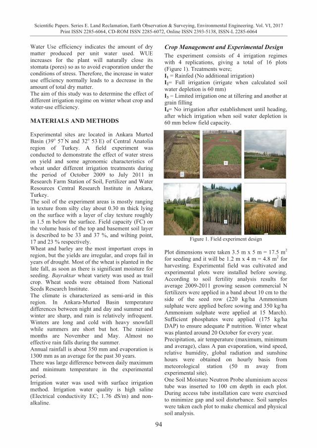
94
Scientific Papers. Series E. Land Reclamation, Earth Observation & Surveying, Environmental Engineering. Vol. VI, 2017Print ISSN 2285-6064, CD-ROM ISSN 2285-6072, Online ISSN 2393-5138, ISSN-L 2285-6064
Water Use efficiency indicates the amount of dry matter produced per unit water used. WUE increases for the plant will naturally close its stomata (pores) so as to avoid evaporation under the conditions of stress. Therefore, the increase in water use efficiency normally leads to a decrease in the amount of total dry matter. The aim of this study was to determine the effect of different irrigation regime on winter wheat crop and water-use efficiency. MATERIALS AND METHODS Experimental sites are located in Ankara Murted Basin (39o 57’N and 32o 53’E) of Central Anatolia region of Turkey. A field experiment was conducted to demonstrate the effect of water stress on yield and some agronomic characteristics of wheat under different irrigation treatments during the period of October 2009 to July 2011 in Research Farm Station of Soil, Fertilizer and Water Resources Central Research Institute in Ankara, Turkey. The soil of the experiment areas is mostly ranging in texture from silty clay about 0.30 m thick lying on the surface with a layer of clay texture roughly in 1.5 m below the surface. Field capacity (FC) on the volume basis of the top and basement soil layer is described to be 33 and 37 %, and wilting point, 17 and 23 % respectively. Wheat and barley are the most important crops in region, but the yields are irregular, and crops fail in years of drought. Most of the wheat is planted in the late fall, as soon as there is significant moisture for seeding. Bayraktar wheat variety was used as trail crop. Wheat seeds were obtained from National Seeds Research Institute. The climate is characterized as semi-arid in this region. In Ankara-Murted Basin temperature differences between night and day and summer and winter are sharp, and rain is relatively infrequent. Winters are long and cold with heavy snowfall while summers are short but hot. The rainiest months are November and May. Almost no effective rain falls during the summer. Annual rainfall is about 350 mm and evaporation is 1300 mm as an average for the past 30 years. There was large difference between daily maximum and minimum temperature in the experimental period. Irrigation water was used with surface irrigation method. Irrigation water quality is high saline (Electrical conductivity EC; 1.76 dS/m) and non-alkaline.
Crop Management and Experimental Design The experiment consists of 4 irrigation regimes with 4 replications, giving a total of 16 plots (Figure 1). Treatments were; I1 = Rainfed (No additional irrigation) I2= Full irrigation (irrigate when calculated soil water depletion is 60 mm) I3 = Limited irrigation one at tillering and another at grain filling I4= No irrigation after establishment until heading, after which irrigation when soil water depletion is 60 mm below field capacity.
Figure 1. Field experiment design Plot dimensions were taken 3.5 m x 5 m = 17.5 m2 for seeding and it will be 1.2 m x 4 m = 4.8 m2 for harvesting. Experimental field was cultivated and experimental plots were installed before sowing. According to soil fertility analysis results for average 2009-2011 growing season commercial N fertilizers were applied in a band about 10 cm to the side of the seed row (220 kg/ha Ammonium sulphate were applied before sowing and 350 kg/ha Ammonium sulphate were applied at 15 March). Sufficient phosphates were applied (175 kg/ha DAP) to ensure adequate P nutrition. Winter wheat was planted around 20 October for every year. Precipitation, air temperature (maximum, minimum and average), class A pan evaporation, wind speed, relative humidity, global radiation and sunshine hours were obtained on hourly basis from meteorological station (50 m away from experimental site). One Soil Moisture Neutron Probe aluminium access tube was inserted to 100 cm depth in each plot. During access tube installation care were exercised to minimize gap and soil disturbance. Soil samples were taken each plot to make chemical and physical soil analysis.
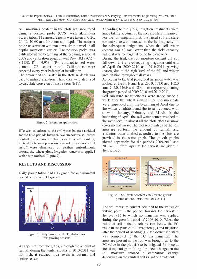
95
Scientific Papers. Series E. Land Reclamation, Earth Observation & Surveying, Environmental Engineering. Vol. VI, 2017Print ISSN 2285-6064, CD-ROM ISSN 2285-6072, Online ISSN 2393-5138, ISSN-L 2285-6064
Water Use efficiency indicates the amount of dry matter produced per unit water used. WUE increases for the plant will naturally close its stomata (pores) so as to avoid evaporation under the conditions of stress. Therefore, the increase in water use efficiency normally leads to a decrease in the amount of total dry matter. The aim of this study was to determine the effect of different irrigation regime on winter wheat crop and water-use efficiency. MATERIALS AND METHODS Experimental sites are located in Ankara Murted Basin (39o 57’N and 32o 53’E) of Central Anatolia region of Turkey. A field experiment was conducted to demonstrate the effect of water stress on yield and some agronomic characteristics of wheat under different irrigation treatments during the period of October 2009 to July 2011 in Research Farm Station of Soil, Fertilizer and Water Resources Central Research Institute in Ankara, Turkey. The soil of the experiment areas is mostly ranging in texture from silty clay about 0.30 m thick lying on the surface with a layer of clay texture roughly in 1.5 m below the surface. Field capacity (FC) on the volume basis of the top and basement soil layer is described to be 33 and 37 %, and wilting point, 17 and 23 % respectively. Wheat and barley are the most important crops in region, but the yields are irregular, and crops fail in years of drought. Most of the wheat is planted in the late fall, as soon as there is significant moisture for seeding. Bayraktar wheat variety was used as trail crop. Wheat seeds were obtained from National Seeds Research Institute. The climate is characterized as semi-arid in this region. In Ankara-Murted Basin temperature differences between night and day and summer and winter are sharp, and rain is relatively infrequent. Winters are long and cold with heavy snowfall while summers are short but hot. The rainiest months are November and May. Almost no effective rain falls during the summer. Annual rainfall is about 350 mm and evaporation is 1300 mm as an average for the past 30 years. There was large difference between daily maximum and minimum temperature in the experimental period. Irrigation water was used with surface irrigation method. Irrigation water quality is high saline (Electrical conductivity EC; 1.76 dS/m) and non-alkaline.
Crop Management and Experimental Design The experiment consists of 4 irrigation regimes with 4 replications, giving a total of 16 plots (Figure 1). Treatments were; I1 = Rainfed (No additional irrigation) I2= Full irrigation (irrigate when calculated soil water depletion is 60 mm) I3 = Limited irrigation one at tillering and another at grain filling I4= No irrigation after establishment until heading, after which irrigation when soil water depletion is 60 mm below field capacity.
Figure 1. Field experiment design Plot dimensions were taken 3.5 m x 5 m = 17.5 m2 for seeding and it will be 1.2 m x 4 m = 4.8 m2 for harvesting. Experimental field was cultivated and experimental plots were installed before sowing. According to soil fertility analysis results for average 2009-2011 growing season commercial N fertilizers were applied in a band about 10 cm to the side of the seed row (220 kg/ha Ammonium sulphate were applied before sowing and 350 kg/ha Ammonium sulphate were applied at 15 March). Sufficient phosphates were applied (175 kg/ha DAP) to ensure adequate P nutrition. Winter wheat was planted around 20 October for every year. Precipitation, air temperature (maximum, minimum and average), class A pan evaporation, wind speed, relative humidity, global radiation and sunshine hours were obtained on hourly basis from meteorological station (50 m away from experimental site). One Soil Moisture Neutron Probe aluminium access tube was inserted to 100 cm depth in each plot. During access tube installation care were exercised to minimize gap and soil disturbance. Soil samples were taken each plot to make chemical and physical soil analysis.
Soil moistures content in the plots was monitored using a neutron probe (CPN) with aluminium access tubes. The measurements were taken at 0-20, 20-40, 40-60 and 60-90cm soil depth. The neutron probe observation was made two times a week in all depths mentioned earlier. The neutron probe was calibrated at the beginning of the growing season at 2008 and calibration equation was PV = 18.195CR + 8.2138, R2 = 0.963** (PV: volumetric soil water content, CR: count ratio). Calibrations were repeated every year before plot installation. The amount of soil water in the 0-90 m depth was used to initiate irrigation. These data were also used to calculate crop evapotranspiration (ETc).
Figure 2. Irrigation application
ETc was calculated as the soil water balance residual for the time periods between two successive soil water content measurement dates. Prior to wheat planting, all trial plots were precision levelled to zero-grade and runoff were eliminated by earthen embankments around the wheat plots. Irrigation water was applied with basin method (Figure 2). RESULTS AND DISCUSSION Daily precipitation and ETo graph for experimental period was given at Figure 2.
Figure 2. Daily rainfall and ETo distribution for growing seasons
As apparent from the graph, although the amount of rainfall during the winter months in 2010-2011 was not high, it reached high levels in autumn and spring season.
According to the plots, irrigation treatments were made taking account of the soil moisture measured. For the full-irrigation plot, the initial soil moisture content value was increased to the field capacity. In the subsequent irrigations, when the soil water content was 60 mm lower than the field capacity value, it was re-irrigated to the field capacity. During the trail, the soil moisture content did not fall down to the level requiring irrigation until end of April for 2009-2010 and 2010-2011 growing season, due to the high level of the fall and winter precipitation throughout all years. According to the trial plots; total irrigation water was applied at the I2, I3 and I4 at 270.0, 171.0 and 162.0 mm, 205.0, 116.0 and 120.0 mm respectively during the growth period of 2009-2010 and 2010-2011. Soil moisture measurements were made twice a week after the wheat sowing. The measurements were suspended until the beginning of April due to the winter conditions and the terrain covered with snow in January, February and March. In the beginning of April, the soil water content reached to the same level in almost all the plots after the snow cover melted away. The measured values of the soil moisture content, the amount of rainfall and irrigation water applied according to the plots are provided in the same graph. The growth graphs plotted separately for the periods 2009-2010 and 2010-2011, from April to the harvest, are given in the Figure 3.
Figure 3. Soil water content data (for the growth
period of 2009-2010 and 2010-2011) The soil moisture content declined to the values of wilting point in the periods towards the harvest in the plot (I1) to which no irrigation was applied during the growth period of 2009-2010. When the value of soil moisture felt 60 mm below the FC value in the plots of full irrigation (I2) and irrigation after the period of heading (I4), the deficit moisture was completed to the FC via irrigation. The moisture present in the soil was brought up to the FC value in the plot (I3) to be irrigated for once at the tilling and grain filling for once. Changes in the soil moisture showed a compatible change depending on the rainfall and irrigation treatments.
F
W
FC-
F
W
FC-60 mm
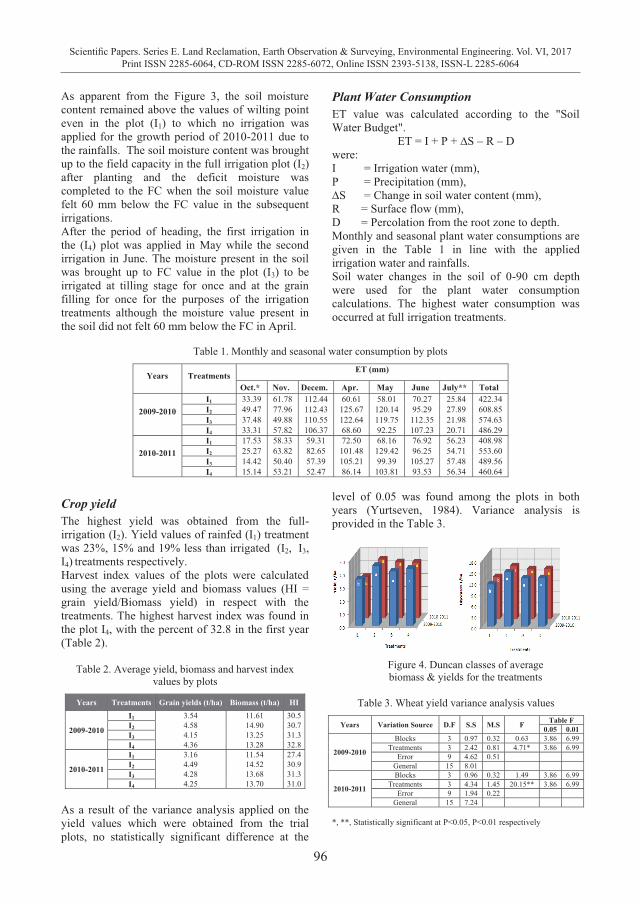
96
Scientific Papers. Series E. Land Reclamation, Earth Observation & Surveying, Environmental Engineering. Vol. VI, 2017Print ISSN 2285-6064, CD-ROM ISSN 2285-6072, Online ISSN 2393-5138, ISSN-L 2285-6064
As apparent from the Figure 3, the soil moisture content remained above the values of wilting point even in the plot (I1) to which no irrigation was applied for the growth period of 2010-2011 due to the rainfalls. The soil moisture content was brought up to the field capacity in the full irrigation plot (I2) after planting and the deficit moisture was completed to the FC when the soil moisture value felt 60 mm below the FC value in the subsequent irrigations. After the period of heading, the first irrigation in the (I4) plot was applied in May while the second irrigation in June. The moisture present in the soil was brought up to FC value in the plot (I3) to be irrigated at tilling stage for once and at the grain filling for once for the purposes of the irrigation treatments although the moisture value present in the soil did not felt 60 mm below the FC in April.
Plant Water Consumption ET value was calculated according to the "Soil Water Budget".
ET = I + P + ∆S – R – D were: I = Irrigation water (mm), P = Precipitation (mm), ∆S = Change in soil water content (mm), R = Surface flow (mm), D = Percolation from the root zone to depth. Monthly and seasonal plant water consumptions are given in the Table 1 in line with the applied irrigation water and rainfalls. Soil water changes in the soil of 0-90 cm depth were used for the plant water consumption calculations. The highest water consumption was occurred at full irrigation treatments.
Table 1. Monthly and seasonal water consumption by plots
Years Treatments ET (mm)
Oct.* Nov. Decem. Apr. May June July** Total
2009-2010 I1 33.39 61.78 112.44 60.61 58.01 70.27 25.84 422.34 I2 49.47 77.96 112.43 125.67 120.14 95.29 27.89 608.85 I3 37.48 49.88 110.55 122.64 119.75 112.35 21.98 574.63 I4 33.31 57.82 106.37 68.60 92.25 107.23 20.71 486.29
2010-2011 I1 17.53 58.33 59.31 72.50 68.16 76.92 56.23 408.98 I2 25.27 63.82 82.65 101.48 129.42 96.25 54.71 553.60 I3 14.42 50.40 57.39 105.21 99.39 105.27 57.48 489.56 I4 15.14 53.21 52.47 86.14 103.81 93.53 56.34 460.64
Crop yield The highest yield was obtained from the full-irrigation (I2). Yield values of rainfed (I1) treatment was 23%, 15% and 19% less than irrigated (I2, I3, I4) treatments respectively. Harvest index values of the plots were calculated using the average yield and biomass values (HI = grain yield/Biomass yield) in respect with the treatments. The highest harvest index was found in the plot I4, with the percent of 32.8 in the first year (Table 2).
Table 2. Average yield, biomass and harvest index values by plots
Years Treatments Grain yields (t/ha) Biomass (t/ha) HI
2009-2010
I1 3.54 11.61 30.5 I2 4.58 14.90 30.7 I3 4.15 13.25 31.3 I4 4.36 13.28 32.8
2010-2011
I1 3.16 11.54 27.4 I2 4.49 14.52 30.9 I3 4.28 13.68 31.3 I4 4.25 13.70 31.0
As a result of the variance analysis applied on the yield values which were obtained from the trial plots, no statistically significant difference at the
level of 0.05 was found among the plots in both years (Yurtseven, 1984). Variance analysis is provided in the Table 3.
Figure 4. Duncan classes of average biomass & yields for the treatments
Table 3. Wheat yield variance analysis values
Years Variation Source D.F S.S M.S F Table F 0.05 0.01
2009-2010
Blocks 3 0.97 0.32 0.63 3.86 6.99 Treatments 3 2.42 0.81 4.71* 3.86 6.99
Error 9 4.62 0.51 General 15 8.01
2010-2011
Blocks 3 0.96 0.32 1.49 3.86 6.99 Treatments 3 4.34 1.45 20.15** 3.86 6.99
Error 9 1.94 0.22 General 15 7.24
*, **, Statistically significant at P<0.05, P<0.01 respectively

97
Scientific Papers. Series E. Land Reclamation, Earth Observation & Surveying, Environmental Engineering. Vol. VI, 2017Print ISSN 2285-6064, CD-ROM ISSN 2285-6072, Online ISSN 2393-5138, ISSN-L 2285-6064
As apparent from the Figure 3, the soil moisture content remained above the values of wilting point even in the plot (I1) to which no irrigation was applied for the growth period of 2010-2011 due to the rainfalls. The soil moisture content was brought up to the field capacity in the full irrigation plot (I2) after planting and the deficit moisture was completed to the FC when the soil moisture value felt 60 mm below the FC value in the subsequent irrigations. After the period of heading, the first irrigation in the (I4) plot was applied in May while the second irrigation in June. The moisture present in the soil was brought up to FC value in the plot (I3) to be irrigated at tilling stage for once and at the grain filling for once for the purposes of the irrigation treatments although the moisture value present in the soil did not felt 60 mm below the FC in April.
Plant Water Consumption ET value was calculated according to the "Soil Water Budget".
ET = I + P + ∆S – R – D were: I = Irrigation water (mm), P = Precipitation (mm), ∆S = Change in soil water content (mm), R = Surface flow (mm), D = Percolation from the root zone to depth. Monthly and seasonal plant water consumptions are given in the Table 1 in line with the applied irrigation water and rainfalls. Soil water changes in the soil of 0-90 cm depth were used for the plant water consumption calculations. The highest water consumption was occurred at full irrigation treatments.
Table 1. Monthly and seasonal water consumption by plots
Years Treatments ET (mm)
Oct.* Nov. Decem. Apr. May June July** Total
2009-2010 I1 33.39 61.78 112.44 60.61 58.01 70.27 25.84 422.34 I2 49.47 77.96 112.43 125.67 120.14 95.29 27.89 608.85 I3 37.48 49.88 110.55 122.64 119.75 112.35 21.98 574.63 I4 33.31 57.82 106.37 68.60 92.25 107.23 20.71 486.29
2010-2011 I1 17.53 58.33 59.31 72.50 68.16 76.92 56.23 408.98 I2 25.27 63.82 82.65 101.48 129.42 96.25 54.71 553.60 I3 14.42 50.40 57.39 105.21 99.39 105.27 57.48 489.56 I4 15.14 53.21 52.47 86.14 103.81 93.53 56.34 460.64
Crop yield The highest yield was obtained from the full-irrigation (I2). Yield values of rainfed (I1) treatment was 23%, 15% and 19% less than irrigated (I2, I3, I4) treatments respectively. Harvest index values of the plots were calculated using the average yield and biomass values (HI = grain yield/Biomass yield) in respect with the treatments. The highest harvest index was found in the plot I4, with the percent of 32.8 in the first year (Table 2).
Table 2. Average yield, biomass and harvest index values by plots
Years Treatments Grain yields (t/ha) Biomass (t/ha) HI
2009-2010
I1 3.54 11.61 30.5 I2 4.58 14.90 30.7 I3 4.15 13.25 31.3 I4 4.36 13.28 32.8
2010-2011
I1 3.16 11.54 27.4 I2 4.49 14.52 30.9 I3 4.28 13.68 31.3 I4 4.25 13.70 31.0
As a result of the variance analysis applied on the yield values which were obtained from the trial plots, no statistically significant difference at the
level of 0.05 was found among the plots in both years (Yurtseven, 1984). Variance analysis is provided in the Table 3.
Figure 4. Duncan classes of average biomass & yields for the treatments
Table 3. Wheat yield variance analysis values
Years Variation Source D.F S.S M.S F Table F 0.05 0.01
2009-2010
Blocks 3 0.97 0.32 0.63 3.86 6.99 Treatments 3 2.42 0.81 4.71* 3.86 6.99
Error 9 4.62 0.51 General 15 8.01
2010-2011
Blocks 3 0.96 0.32 1.49 3.86 6.99 Treatments 3 4.34 1.45 20.15** 3.86 6.99
Error 9 1.94 0.22 General 15 7.24
*, **, Statistically significant at P<0.05, P<0.01 respectively
In the Duncan test, two different groups emerged for the years 2009-2010 and 2010-2011. No class difference was found between the plots I2, I3 and I4 and all took part in the first group. The no-irrigation plot I1 constituted the second group. The classification concerning the Duncan Test results were given on the Figure 4. The reason why there is no group difference between the irrigation plots is that spring and winter precipitation was high in both years. Water Use Efficiency (WUE) WUE values calculated according to the years when the trial was carried out are given in the Table 4. It was reported that in general, the wheat WUE ranges from 4.0 to 18.3 kg/ha/mm globally on a yield basis (Anderson, 1992; Oweis et al., 2000).
Table 4. WUE values by plots
Years Treatments ET (mm)
Yields (t/ha)
Irrigation (mm)
WUE (kg/m3)
2009-2010
I1 422 3.54 - 8.38b
I2 609 4.58 290 7.52 b I3 575 4.15 183 7.22 b I4 486 4.36 162 8.97 a
2010-2011
I1 409 3.16 - 7.72 b I2 554 4.49 205 8.10 b I3 490 4.28 120 8.73 b I4 461 4.25 104 9.22 a
As for the WUE in 2009-2010, the best outcome was provided by the plot I4 (irrigation when the soil water potential diminished 60 mm beginning from the period of heading stage). It was respectively followed by I1 (no-irrigation) and I2 (full irrigation). The water use had the lowest efficiency in the plot I3 (irrigation in which the moisture present in the soil was brought up to the field capacity was applied for once at the tilling stage and at the grain filling stage for once). For the growth period of 2010-2011, WUE was in the plot I4 with a value of 9.2 kg/m3 and it was respectively followed by I3, I2 and I1 with the values of 8.7, 8.1 and 7.7 kg/m3. The more effective water-use in winter wheat crop was obtained with treatment I4 (no irrigation until heading, after will irrigate calculated soil water depletion is 60 mm). CONCLUSION Efforts to get more crops per unit area are quite important and necessary for human nutrition in today’s world having limited resources as well as a rapidly growing population.
At the end of the research study conducted during the wheat growth period for the years 2009-2010 and 2010-2011 in average wheat yield was found to be 3.35 t/ha, 4.54 t/ha, 4.22 t/ha and 4.31 t/ha respectively according to the plots (I1, I2, I3, I4). The highest yield was obtained from the full-irrigation plot while the lowest yield was obtained from the no-irrigation plot. No statistically significant difference was found between the plots subjected to the irrigation treatments while a difference of P < 0.05 was obtained between the no-irrigation and full-irrigation plots. Average harvest index values were found to be respectively 29%, 31%, 32% 31% and 32% again according to the plots. The plot I4 that was irrigated in the same way after the period of heading for both years appeared to have the highest value in the water use efficiency. It might be recommended that irrigation concentrated in the after heading period increase WUE in Central Anatolia Region of Turkey. ACKNOWLEDGMENTS We gratefully acknowledge the technical and financial support of the International Atomic Energy Agency through the research contract number TUR/14463 and Scientific and Technological Research Council of Turkey, project number TÜBİTAK 1001/108O654. Special appreciation is given to the Soil Fertilizer and Water Resources Central Research Institute for providing the labour and land for this experiment. REFERENCES Anderson W.K., 1992. Increasing grain yield and water
use of wheat in rainfed Mediterranean type environment. Australian Journal of Agricultural Resources, 43:1-17.
Barnett T. P., Adam J. C., Lettenmaier D. P., 2005. Potential impacts of a warming climate on water availability in snow-dominated regions. Nature, 438, 303-309.
Clay D.E., Engel R.E., Long S., Liu Z., 2001. Nitrogen and water stress interact to influence Carbon-13 discrimination in wheat. Soil Science Society of American Journal, 65; 1823-1828.
Oweis T., Zhang H., Pala M., 2000. Water Use Efficiency of Rainfed and Irrigated Bread Wheat in a Mediterranean Environment. Agronomy Journal, Vol. 92; 231-238.
Yurtsever N., 1984. Experimental Statistical methods. General Directorate of Rural Services. Publication, 121-123.
98
Scientific Papers. Series E. Land Reclamation, Earth Observation & Surveying, Environmental Engineering. Vol. VI, 2017Print ISSN 2285-6064, CD-ROM ISSN 2285-6072, Online ISSN 2393-5138, ISSN-L 2285-6064
COMPARISON BETWEEN TWO PRODUCTION
TECHNOLOGIES AND TWO TYPES OF SUBSTRATES IN AN EXPERIMENTAL AQUAPONIC RECIRCULATION SYSTEM
Ivaylo SIRAKOV1, Katya VELICHKOVA1, Stefka STOYANOVA1,
Desislava SLAVCHEVA-SIRAKOVA2, Yordan STAYKOV1
1Trakia University, Studetski grad, 6000 Stara Zagora, Bulgaria
2Agricultural University, 12 Mendeleev Blvd., 4000 Plovdiv, Bulgaria
Corresponding author email: [email protected] Abstract Two of the main parameters, which defined the cleaning capacity of cultivated plants and productivity of aquaponic systems, are the type of hydroponic compartment and plant’s growing media. The aim of current research was to compare the cleaning capacity and plant’s productivity of media bed and raft hydroponic sections as a part of a model aquaponic recirculation system. The impact of different plant growing mediums (cotton wool and rockwool) on lettuce yields was also retraced. For the purpose of this research two types of hydroponic sections (media bed and deep water sections) were constructed and integrated into an existing recirculation aquaculture system. For the trial 36 lettuce seedlings were used. Half of the plants were transferred to cotton wool and the other half of the lettuce plants were transferred to rockwool (Grodan®) substrates and afterwards all plants were placed in hydroponic pots. Eighteen lettuce seedlings (half planted on cotton wool and the other half on rockwool (Grodan®) substrate) were planted on the hydroponic section filled with lightweight expanded clay aggregate (LECA) and the other eighteen plants (half planted on cotton wool and the other half on rockwool (Grodan®) substrate) were planted on the floating raft hydroponic section.The hydrochemical parameters were measured during the trial. At the end and middle of the trial the fresh weight of lettuce plants was measured.A better removal capacity in ammonium, nitrate and ortho-phospahte were observed in the LECA section compared with the cleaning capacity in the raft section as a part of experimental aquaponic system. The raft technology showed better plant productivity compared with the one found for the LECA bed technology. The productivity of lettuce plants is highly dependent on the type of plant growing medium, when they are cultivated in the floating raft technology. Key words: aquaponic, deep water technology, media bed technology, plant growing substrates INTRODUCTION Aquaponics is a sustainable aquaculture technology (Nelson, 2007; Graber and Junge, 2009; Diver and Rinehart, 2010), where the hydrobionts and vegetables are cultivated in the same recirculation system (Rakocy et al, 2006; Timmons et al., 2002; Rakocy et al, 2006; Karimanzira et al., 2016). The interest of the aquaculture sector in Bulgaria on this particular production techno-logy is continuously increasing in the last few years. Some aquaponics projects were already accepted for financing from “Programme for Maritime Affairs and fisheries /2014-2020/”. Although studies connected to the development of aquaponic technology in Bulgaria will be highly appreciated by the aquaculture branch, such studies are still missingup to now.
As an innovative technology the efforts of many researchers are connected to the optimization of aquaponics. Two of the main parameters, which defined the cleaning capacity of cultivated plants and productivity of aquaponics systems, are the type of hydroponic compartment and plant’s growing media. Limited studies are connected with these topics (Lennard and Leonard, 2006; Roosta and Afsharipoor, 2012; Schmautz et al., 2016), and many research questions still remain open. The aim of current research was to compare the cleaning capacity and plant’s productivity of media bed and raft hydroponic sections as a part of a model aquaponic recirculation system. The impact of different plant growing mediums (cotton wool and rock wool) on lettuce yields was also retraced.
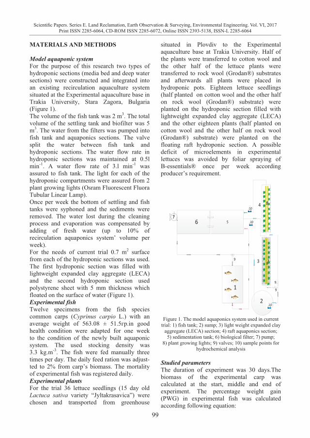
99
Scientific Papers. Series E. Land Reclamation, Earth Observation & Surveying, Environmental Engineering. Vol. VI, 2017Print ISSN 2285-6064, CD-ROM ISSN 2285-6072, Online ISSN 2393-5138, ISSN-L 2285-6064
COMPARISON BETWEEN TWO PRODUCTION
TECHNOLOGIES AND TWO TYPES OF SUBSTRATES IN AN EXPERIMENTAL AQUAPONIC RECIRCULATION SYSTEM
Ivaylo SIRAKOV1, Katya VELICHKOVA1, Stefka STOYANOVA1,
Desislava SLAVCHEVA-SIRAKOVA2, Yordan STAYKOV1
1Trakia University, Studetski grad, 6000 Stara Zagora, Bulgaria
2Agricultural University, 12 Mendeleev Blvd., 4000 Plovdiv, Bulgaria
Corresponding author email: [email protected] Abstract Two of the main parameters, which defined the cleaning capacity of cultivated plants and productivity of aquaponic systems, are the type of hydroponic compartment and plant’s growing media. The aim of current research was to compare the cleaning capacity and plant’s productivity of media bed and raft hydroponic sections as a part of a model aquaponic recirculation system. The impact of different plant growing mediums (cotton wool and rockwool) on lettuce yields was also retraced. For the purpose of this research two types of hydroponic sections (media bed and deep water sections) were constructed and integrated into an existing recirculation aquaculture system. For the trial 36 lettuce seedlings were used. Half of the plants were transferred to cotton wool and the other half of the lettuce plants were transferred to rockwool (Grodan®) substrates and afterwards all plants were placed in hydroponic pots. Eighteen lettuce seedlings (half planted on cotton wool and the other half on rockwool (Grodan®) substrate) were planted on the hydroponic section filled with lightweight expanded clay aggregate (LECA) and the other eighteen plants (half planted on cotton wool and the other half on rockwool (Grodan®) substrate) were planted on the floating raft hydroponic section.The hydrochemical parameters were measured during the trial. At the end and middle of the trial the fresh weight of lettuce plants was measured.A better removal capacity in ammonium, nitrate and ortho-phospahte were observed in the LECA section compared with the cleaning capacity in the raft section as a part of experimental aquaponic system. The raft technology showed better plant productivity compared with the one found for the LECA bed technology. The productivity of lettuce plants is highly dependent on the type of plant growing medium, when they are cultivated in the floating raft technology. Key words: aquaponic, deep water technology, media bed technology, plant growing substrates INTRODUCTION Aquaponics is a sustainable aquaculture technology (Nelson, 2007; Graber and Junge, 2009; Diver and Rinehart, 2010), where the hydrobionts and vegetables are cultivated in the same recirculation system (Rakocy et al, 2006; Timmons et al., 2002; Rakocy et al, 2006; Karimanzira et al., 2016). The interest of the aquaculture sector in Bulgaria on this particular production techno-logy is continuously increasing in the last few years. Some aquaponics projects were already accepted for financing from “Programme for Maritime Affairs and fisheries /2014-2020/”. Although studies connected to the development of aquaponic technology in Bulgaria will be highly appreciated by the aquaculture branch, such studies are still missingup to now.
As an innovative technology the efforts of many researchers are connected to the optimization of aquaponics. Two of the main parameters, which defined the cleaning capacity of cultivated plants and productivity of aquaponics systems, are the type of hydroponic compartment and plant’s growing media. Limited studies are connected with these topics (Lennard and Leonard, 2006; Roosta and Afsharipoor, 2012; Schmautz et al., 2016), and many research questions still remain open. The aim of current research was to compare the cleaning capacity and plant’s productivity of media bed and raft hydroponic sections as a part of a model aquaponic recirculation system. The impact of different plant growing mediums (cotton wool and rock wool) on lettuce yields was also retraced.
MATERIALS AND METHODS Model aquaponic system For the purpose of this research two types of hydroponic sections (media bed and deep water sections) were constructed and integrated into an existing recirculation aquaculture system situated at the Experimental aquaculture base in Trakia University, Stara Zagora, Bulgaria (Figure 1). The volume of the fish tank was 2 m3. The total volume of the settling tank and biofilter was 5 m3. The water from the filters was pumped into fish tank and aquaponics sections. The valve split the water between fish tank and hydroponic sections. The water flow rate in hydroponic sections was maintained at 0.5l min-1. A water flow rate of 3.l min-1 was assured to fish tank. The light for each of the hydroponic compartments were assured from 2 plant growing lights (Osram Fluorescent Fluora Tubular Linear Lamp). Once per week the bottom of settling and fish tanks were syphoned and the sediments were removed. The water lost during the cleaning process and evaporation was compensated by adding of fresh water (up to 10% of recirculation aquaponics system’ volume per week). For the needs of current trial 0.7 m2 surface from each of the hydroponic sections was used. The first hydroponic section was filled with lightweight expanded clay aggregate (LECA) and the second hydroponic section used polystyrene sheet with 5 mm thickness which floated on the surface of water (Figure 1). Experimental fish Twelve specimens from the fish species common carps (Cyprinus carpio L.) with an average weight of 563.08 ± 51.5гр.in good health condition were adapted for one week to the condition of the newly built aquaponic system. The used stocking density was 3.3 kg.m-3. The fish were fed manually three times per day. The daily feed ration was adjust-ted to 2% from carp’s biomass. The mortality of experimental fish was registered daily. Experimental plants For the trial 36 lettuce seedlings (15 day old Lactuca sativa variety “Jyltakrasavica”) were chosen and transported from greenhouse
situated in Plovdiv to the Experimental aquaculture base at Trakia University. Half of the plants were transferred to cotton wool and the other half of the lettuce plants were transferred to rock wool (Grodan®) substrates and afterwards all plants were placed in hydroponic pots. Eighteen lettuce seedlings (half planted on cotton wool and the other half on rock wool (Grodan®) substrate) were planted on the hydroponic section filled with lightweight expanded clay aggregate (LECA) and the other eighteen plants (half planted on cotton wool and the other half on rock wool (Grodan®) substrate) were planted on the floating raft hydroponic section. A possible deficit of microelements in experimental lettuces was avoided by foliar spraying of B-essentials® once per week according producer’s requirement.
1
2
567
333333333333333333333333333333333333333333333333333333333333333333333333333333333333333333333333333333333333333333333333333333333333333333333
4
3
8
8
9
9
9
10
10
10
Figure 1. The model aquaponics system used in current trial: 1) fish tank; 2) sump; 3) light weight expanded clay
aggregate (LECA) section; 4) raft aquaponics section; 5) sedimentation tank; 6) biological filter; 7) pump;
8) plant growing lights; 9) valves; 10) sample points for hydrochemical analysis
Studied parameters The duration of experiment was 30 days.The biomass of the experimental carp was calculated at the start, middle and end of experiment. The percentage weight gain (PWG) in experimental fish was calculated according following equation:
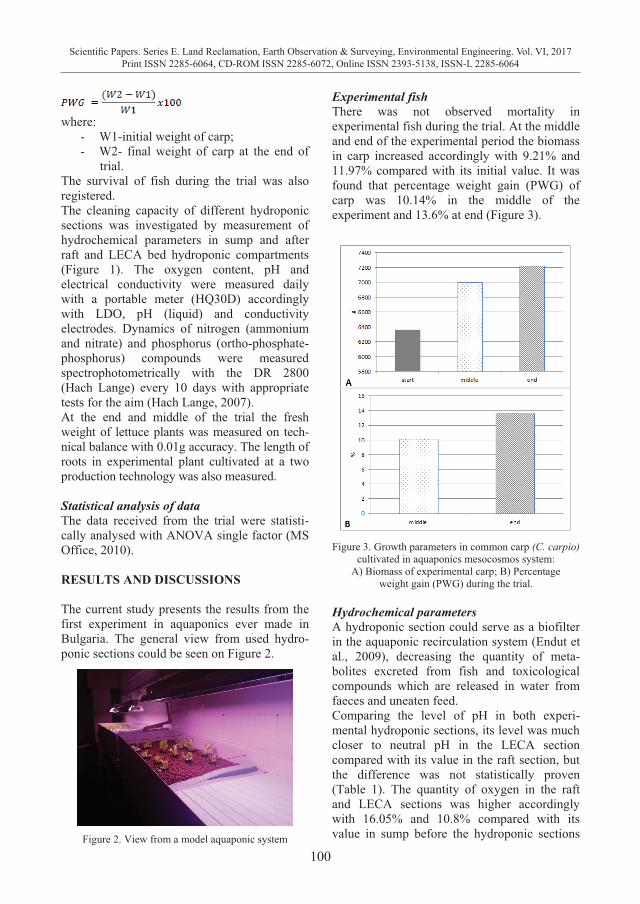
100
Scientific Papers. Series E. Land Reclamation, Earth Observation & Surveying, Environmental Engineering. Vol. VI, 2017Print ISSN 2285-6064, CD-ROM ISSN 2285-6072, Online ISSN 2393-5138, ISSN-L 2285-6064
where:
- W1-initial weight of carp; - W2- final weight of carp at the end of
trial. The survival of fish during the trial was also registered. The cleaning capacity of different hydroponic sections was investigated by measurement of hydrochemical parameters in sump and after raft and LECA bed hydroponic compartments (Figure 1). The oxygen content, pH and electrical conductivity were measured daily with a portable meter (HQ30D) accordingly with LDO, pH (liquid) and conductivity electrodes. Dynamics of nitrogen (ammonium and nitrate) and phosphorus (ortho-phosphate-phosphorus) compounds were measured spectrophotometrically with the DR 2800 (Hach Lange) every 10 days with appropriate tests for the aim (Hach Lange, 2007).At the end and middle of the trial the fresh weight of lettuce plants was measured on tech-nical balance with 0.01g accuracy. The length of roots in experimental plant cultivated at a two production technology was also measured. Statistical analysis of data The data received from the trial were statisti-cally analysed with ANOVA single factor (MS Office, 2010). RESULTS AND DISCUSSIONS The current study presents the results from the first experiment in aquaponics ever made in Bulgaria. The general view from used hydro-ponic sections could be seen on Figure 2.
Figure 2. View from a model aquaponic system
Experimental fish There was not observed mortality in experimental fish during the trial. At the middle and end of the experimental period the biomass in carp increased accordingly with 9.21% and 11.97% compared with its initial value. It was found that percentage weight gain (PWG) of carp was 10.14% in the middle of the experiment and 13.6% at end (Figure 3).
Figure 3. Growth parameters in common carp (C. carpio)
cultivated in aquaponics mesocosmos system: A) Biomass of experimental carp; B) Percentage
weight gain (PWG) during the trial. Hydrochemical parameters A hydroponic section could serve as a biofilter in the aquaponic recirculation system (Endut et al., 2009), decreasing the quantity of meta-bolites excreted from fish and toxicological compounds which are released in water from faeces and uneaten feed. Comparing the level of pH in both experi-mental hydroponic sections, its level was much closer to neutral pH in the LECA section compared with its value in the raft section, but the difference was not statistically proven (Table 1). The quantity of oxygen in the raft and LECA sections was higher accordingly with 16.05% and 10.8% compared with its value in sump before the hydroponic sections
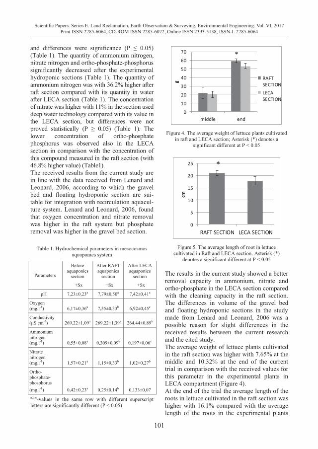
101
Scientific Papers. Series E. Land Reclamation, Earth Observation & Surveying, Environmental Engineering. Vol. VI, 2017Print ISSN 2285-6064, CD-ROM ISSN 2285-6072, Online ISSN 2393-5138, ISSN-L 2285-6064
where:
- W1-initial weight of carp; - W2- final weight of carp at the end of
trial. The survival of fish during the trial was also registered. The cleaning capacity of different hydroponic sections was investigated by measurement of hydrochemical parameters in sump and after raft and LECA bed hydroponic compartments (Figure 1). The oxygen content, pH and electrical conductivity were measured daily with a portable meter (HQ30D) accordingly with LDO, pH (liquid) and conductivity electrodes. Dynamics of nitrogen (ammonium and nitrate) and phosphorus (ortho-phosphate-phosphorus) compounds were measured spectrophotometrically with the DR 2800 (Hach Lange) every 10 days with appropriate tests for the aim (Hach Lange, 2007).At the end and middle of the trial the fresh weight of lettuce plants was measured on tech-nical balance with 0.01g accuracy. The length of roots in experimental plant cultivated at a two production technology was also measured. Statistical analysis of data The data received from the trial were statisti-cally analysed with ANOVA single factor (MS Office, 2010). RESULTS AND DISCUSSIONS The current study presents the results from the first experiment in aquaponics ever made in Bulgaria. The general view from used hydro-ponic sections could be seen on Figure 2.
Figure 2. View from a model aquaponic system
Experimental fish There was not observed mortality in experimental fish during the trial. At the middle and end of the experimental period the biomass in carp increased accordingly with 9.21% and 11.97% compared with its initial value. It was found that percentage weight gain (PWG) of carp was 10.14% in the middle of the experiment and 13.6% at end (Figure 3).
Figure 3. Growth parameters in common carp (C. carpio)
cultivated in aquaponics mesocosmos system: A) Biomass of experimental carp; B) Percentage
weight gain (PWG) during the trial. Hydrochemical parameters A hydroponic section could serve as a biofilter in the aquaponic recirculation system (Endut et al., 2009), decreasing the quantity of meta-bolites excreted from fish and toxicological compounds which are released in water from faeces and uneaten feed. Comparing the level of pH in both experi-mental hydroponic sections, its level was much closer to neutral pH in the LECA section compared with its value in the raft section, but the difference was not statistically proven (Table 1). The quantity of oxygen in the raft and LECA sections was higher accordingly with 16.05% and 10.8% compared with its value in sump before the hydroponic sections
and differences were significance (P ≤ 0.05) (Table 1). The quantity of ammonium nitrogen, nitrate nitrogen and ortho-phosphate-phosphorus significantly decreased after the experimental hydroponic sections (Table 1). The quantity of ammonium nitrogen was with 36.2% higher after raft section compared with its quantity in water after LECA section (Table 1). The concentration of nitrate was higher with 11% in the section used deep water technology compared with its value in the LECA section, but differences were not proved statistically (P ≥ 0.05) (Table 1). The lower concentration of ortho-phosphate phosphorus was observed also in the LECA section in comparison with the concentration of this compound measured in the raft section (with 46.8% higher value) (Table1). The received results from the current study are in line with the data received from Lenard and Leonard, 2006, according to which the gravel bed and floating hydroponic section are sui-table for integration with recirculation aquacul-ture system. Lenard and Leonard, 2006, found that oxygen concentration and nitrate removal was higher in the raft system but phosphate removal was higher in the gravel bed section.
Table 1. Hydrochemical parameters in mesocosmos aquaponics system
Parameters
Before aquaponics
section
+Sx
After RAFT aquaponics
section
+Sx
After LECA aquaponics
section
+Sx
pH 7,23±0,23a 7,79±0,50a 7,42±0,41a
Oxygen (mg.l-1) 6,17±0,36a 7,35±0,33b 6,92±0,45c
Conductivity (µS.cm-3) 269,22±1,09a 269,22±1,39a 264,44±0,89b
Ammonium nitrogen (mg.l-1) 0,55±0,08a 0,309±0,09b 0,197±0,06c
Nitrate nitrogen (mg.l-1) 1,57±0,21a 1,15±0,33b 1,02±0,27b
Ortho-phosphate-phosphorus (mg.l-1) 0,42±0,23a 0,25±0,14b 0,133±0,07 a,b,c-values in the same row with different superscript letters are significantly different (P < 0.05)
*
0
10
20
30
40
50
60
70
middle end
g RAFTSECTIONLECASECTION
Figure 4. The average weight of lettuce plants cultivated
in raft and LECA section; Asterisk (*) denotes a significant different at P < 0.05
*
0
5
10
15
20
25
RAFT SECTION LECA SECTION
сm
Figure 5. The average length of root in lettuce
cultivated in Raft and LECA section. Asterisk (*) denotes a significant different at P < 0.05
The results in the current study showed a better removal capacity in ammonium, nitrate and ortho-phosphate in the LECA section compared with the cleaning capacity in the raft section. The differences in volume of the gravel bed and floating hydroponic sections in the study made from Lenard and Leonard, 2006 was a possible reason for slight differences in the received results between the current research and the cited study. The average weight of lettuce plants cultivated in the raft section was higher with 7.65% at the middle and 10.32% at the end of the current trial in comparison with the received values for this parameter in the experimental plants in LECA compartment (Figure 4). At the end of the trial the average length of the roots in lettuce cultivated in the raft section was higher with 16.1% compared with the average length of the roots in the experimental plants
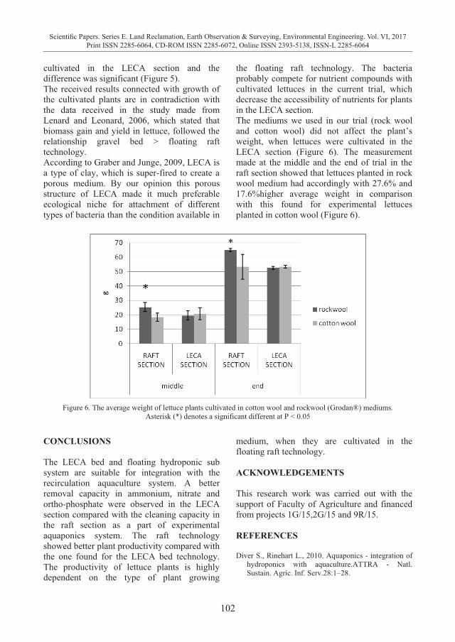
102
Scientific Papers. Series E. Land Reclamation, Earth Observation & Surveying, Environmental Engineering. Vol. VI, 2017Print ISSN 2285-6064, CD-ROM ISSN 2285-6072, Online ISSN 2393-5138, ISSN-L 2285-6064
cultivated in the LECA section and the difference was significant (Figure 5). The received results connected with growth of the cultivated plants are in contradiction with the data received in the study made from Lenard and Leonard, 2006, which stated that biomass gain and yield in lettuce, followed the relationship gravel bed > floating raft technology. According to Graber and Junge, 2009, LECA is a type of clay, which is super-fired to create a porous medium. By our opinion this porous structure of LECA made it much preferable ecological niche for attachment of different types of bacteria than the condition available in
the floating raft technology. The bacteria probably compete for nutrient compounds with cultivated lettuces in the current trial, which decrease the accessibility of nutrients for plants in the LECA section. The mediums we used in our trial (rock wool and cotton wool) did not affect the plant’s weight, when lettuces were cultivated in the LECA section (Figure 6). The measurement made at the middle and the end of trial in the raft section showed that lettuces planted in rock wool medium had accordingly with 27.6% and 17.6%higher average weight in comparison with this found for experimental lettuces planted in cotton wool (Figure 6).
Figure 6. The average weight of lettuce plants cultivated in cotton wool and rockwool (Grodan®) mediums.
Asterisk (*) denotes a significant different at P < 0.05
CONCLUSIONS The LECA bed and floating hydroponic sub system are suitable for integration with the recirculation aquaculture system. A better removal capacity in ammonium, nitrate and ortho-phosphate were observed in the LECA section compared with the cleaning capacity in the raft section as a part of experimental aquaponics system. The raft technology showed better plant productivity compared with the one found for the LECA bed technology. The productivity of lettuce plants is highly dependent on the type of plant growing
medium, when they are cultivated in the floating raft technology. ACKNOWLEDGEMENTS This research work was carried out with the support of Faculty of Agriculture and financed from projects 1G/15,2G/15 and 9R/15. REFERENCES Diver S., Rinehart L., 2010. Aquaponics - integration of
hydroponics with aquaculture.ATTRA - Natl. Sustain. Agric. Inf. Serv.28:1–28.
103
Scientific Papers. Series E. Land Reclamation, Earth Observation & Surveying, Environmental Engineering. Vol. VI, 2017Print ISSN 2285-6064, CD-ROM ISSN 2285-6072, Online ISSN 2393-5138, ISSN-L 2285-6064
cultivated in the LECA section and the difference was significant (Figure 5). The received results connected with growth of the cultivated plants are in contradiction with the data received in the study made from Lenard and Leonard, 2006, which stated that biomass gain and yield in lettuce, followed the relationship gravel bed > floating raft technology. According to Graber and Junge, 2009, LECA is a type of clay, which is super-fired to create a porous medium. By our opinion this porous structure of LECA made it much preferable ecological niche for attachment of different types of bacteria than the condition available in
the floating raft technology. The bacteria probably compete for nutrient compounds with cultivated lettuces in the current trial, which decrease the accessibility of nutrients for plants in the LECA section. The mediums we used in our trial (rock wool and cotton wool) did not affect the plant’s weight, when lettuces were cultivated in the LECA section (Figure 6). The measurement made at the middle and the end of trial in the raft section showed that lettuces planted in rock wool medium had accordingly with 27.6% and 17.6%higher average weight in comparison with this found for experimental lettuces planted in cotton wool (Figure 6).
Figure 6. The average weight of lettuce plants cultivated in cotton wool and rockwool (Grodan®) mediums.
Asterisk (*) denotes a significant different at P < 0.05
CONCLUSIONS The LECA bed and floating hydroponic sub system are suitable for integration with the recirculation aquaculture system. A better removal capacity in ammonium, nitrate and ortho-phosphate were observed in the LECA section compared with the cleaning capacity in the raft section as a part of experimental aquaponics system. The raft technology showed better plant productivity compared with the one found for the LECA bed technology. The productivity of lettuce plants is highly dependent on the type of plant growing
medium, when they are cultivated in the floating raft technology. ACKNOWLEDGEMENTS This research work was carried out with the support of Faculty of Agriculture and financed from projects 1G/15,2G/15 and 9R/15. REFERENCES Diver S., Rinehart L., 2010. Aquaponics - integration of
hydroponics with aquaculture.ATTRA - Natl. Sustain. Agric. Inf. Serv.28:1–28.
Graber A., Junge R., 2009. Aquaponic Systems: Nutrient recycling from fish wastewater by vegetable production. Desalination 246 (1): 147-156.
Hach Lange, 2007. DR 2800 Spectrophotometer-procedures manual, Ed. 2, Germany, 814 pp.
Karimanzira D., Keesman K. J., Kloas W., Baganz D., Rauschenbach T., 2016. Dynamic modeling of the INAPRO aquaponic system. Aquacultural Engineering, 75, 29-45.
Lennard W. A., Leonard, B. V.,2006. A comparison of three different hydroponic sub-systems (gravel bed, floating and nutrient film technique) in an Aquaponictest system. Aquaculture International, 14(6), 539-550.
Nelson R.L., 2007. Ten aquaponic systems around the world. Aquaponics J. 46:8–12.
Rakocy J.E., Massor M.P., Losordo T.M., 2006. Recirculating Aquaculture Tank Production Systems:
Aquaponics—Integrating Fish and Plant Culture. SRAC Publication No. 454, 16pp.
Roosta, H. R., Afsharipoor S., 2012. Effects of different cultivation media on vegetative growth, ecophysiolocal traits and nutrients concentration in strawberry under hydroponic and aquaponic cultivation systems. Advances in Environmental Biology, Jaipur, v.6, n.2, p.543-555.
Schmautz Z., Loeu F., Liebisch F., Graber A., Mathis A., Griessler Bulc, T., Junge, R., 2016. Tomato Productivity and Quality in Aquaponics: Comparison of Three Hydroponic Methods. Water, 8(11), 533.
Timmons M., Ebeling, J., Wheaton F., Summerfelt S., Vinci B. 2002. Recirculating aquaculture systems, 2nd edition. North East Reg. Aquaculture Ctr. Pub. No. 01–002.
104
Scientific Papers. Series E. Land Reclamation, Earth Observation & Surveying, Environmental Engineering. Vol. VI, 2017Print ISSN 2285-6064, CD-ROM ISSN 2285-6072, Online ISSN 2393-5138, ISSN-L 2285-6064
BIOACUMULATION AND PROTEIN CONTENT
OF LEMNA MINUTA KUNTH AND LEMNA VALDIVIANA PHIL. IN BULGARIAN WATER RESERVOIRS
Katya VELICHKOVA, Ivaylo SIRAKOV, Elica VALKOVA, Stefka STOYANOVA,
Gergana KOSTADINOVA
Trakia University, Students Campus, 6000 Stara Zagora, Bulgaria
Corresponding author email: [email protected] Abstract Lemna sp. have an important role indifferent aspect of aquatic ecosystems serving as a food source, by providing shelter to fish and aquatic invertebrates, changing water quality by regulating oxygen balance, nutrient cycles, and accumulating heavy metals.The aim of present study was to investigate a new found species of Lemna in Bulgarian water reservoirs regarding their protein content and bioaccumulation of heavy metals. Two water bodies located on the territory of South East Bulgaria –Tvardica Dam Lake with growing L. minuta and Nikolaevo fishpond with growing L. valdiviana were studied. Crude protein, lipid, ash contentin two species of Lemna were analysed. The heavy metal in water andaquatic plants was determined on an atomic absorption spectrometer (AAS) "A Analyst 800" - Perkin Elmer. The highest quantity of protein was measured in L. minuta (26.42%), which was 8.71% more compared to L. valdiviana (24.12). The concentrations of metals in the L. minuta and L. valdiviana followed a downward trend: Mn>Fe>Zn>Cu>Ni>Cr>Pb>Cd. The series of bioaccumulation is in descending order: Mn>Fe>Cu>Zn>Cr> Cd>Pb>Ni for L. minuta, and Mn>Fe>Zn>Cu>Cd>Pb>Cr>Ni for L. valdiviana. Key words: bioaccumulation, heavy metal, Lemna minuta, Lemna valdiviana, protein. INTRODUCTION The increasing population and rapid industrialization, fertilizer and pesticide use led to an increased anthropogenic impact on the environment. These contaminants diffuse into aquatic environments through industrial discharges, petroleum spills, urban and atmospheric fall-out (Olajire et al., 2005). The heavy metals are of major importance among various water pollutants because of their persistent and bio-accumulative nature (Chang et al., 2009; Yadav et al., 2009). Most of the heavy metals are toxic in nature and can be a threat to human health and the environment at higher concentrations (Vinodhini and Narayanan, 2009). Copper (Cu), nickel (Ni), cadmium (Cd) and zinc (Zn) are considered as toxic since they cause deleterious effect in plants, animals and humans (Chaudhary and Sharma, 2014). Water as vital for people is need to develop a low cost and eco-friendly technology to remove pollutants particularly heavy metals, thereby improving water quality. Conventional remediation systems based on
physical and chemical methods are efficient but have economical and technical limitation. Bioaccumulation of various heavy metals in aquatic and wetland ecosystems has important significance globally (Greger, 1999). Some aquatic macrophytes take up heavy metals from aquatic environment and are being used in wastewater renovation systems (Prasad et al., 2001). Such an excellent candidate for removal, disposal, and recovery of heavymetals from the polluted aquatic ecosystems is Lemna sp. These free-floating, fast growing, and nitrogen fixing pteridophyte also have a higher content of protein. Lemna sp. are found in temperate climates and serve as an important food source for various water birds and fish (Drost et al., 2007). Lemna sp. have an important role indifferent aspect of aquatic ecosystems serving as a food source, by providing shelter to fish and aquatic invertebrates, changing water quality by regulating oxygen balance, nutrient cycles, and accumulating heavy metals. The protein content of Lemna sp. is one of the highest in the plant kingdom - 6.8 – 45.0 (Lehmanet al., 1981; Landolt and Kandeler,
105
Scientific Papers. Series E. Land Reclamation, Earth Observation & Surveying, Environmental Engineering. Vol. VI, 2017Print ISSN 2285-6064, CD-ROM ISSN 2285-6072, Online ISSN 2393-5138, ISSN-L 2285-6064
BIOACUMULATION AND PROTEIN CONTENT
OF LEMNA MINUTA KUNTH AND LEMNA VALDIVIANA PHIL. IN BULGARIAN WATER RESERVOIRS
Katya VELICHKOVA, Ivaylo SIRAKOV, Elica VALKOVA, Stefka STOYANOVA,
Gergana KOSTADINOVA
Trakia University, Students Campus, 6000 Stara Zagora, Bulgaria
Corresponding author email: [email protected] Abstract Lemna sp. have an important role indifferent aspect of aquatic ecosystems serving as a food source, by providing shelter to fish and aquatic invertebrates, changing water quality by regulating oxygen balance, nutrient cycles, and accumulating heavy metals.The aim of present study was to investigate a new found species of Lemna in Bulgarian water reservoirs regarding their protein content and bioaccumulation of heavy metals. Two water bodies located on the territory of South East Bulgaria –Tvardica Dam Lake with growing L. minuta and Nikolaevo fishpond with growing L. valdiviana were studied. Crude protein, lipid, ash contentin two species of Lemna were analysed. The heavy metal in water andaquatic plants was determined on an atomic absorption spectrometer (AAS) "A Analyst 800" - Perkin Elmer. The highest quantity of protein was measured in L. minuta (26.42%), which was 8.71% more compared to L. valdiviana (24.12). The concentrations of metals in the L. minuta and L. valdiviana followed a downward trend: Mn>Fe>Zn>Cu>Ni>Cr>Pb>Cd. The series of bioaccumulation is in descending order: Mn>Fe>Cu>Zn>Cr> Cd>Pb>Ni for L. minuta, and Mn>Fe>Zn>Cu>Cd>Pb>Cr>Ni for L. valdiviana. Key words: bioaccumulation, heavy metal, Lemna minuta, Lemna valdiviana, protein. INTRODUCTION The increasing population and rapid industrialization, fertilizer and pesticide use led to an increased anthropogenic impact on the environment. These contaminants diffuse into aquatic environments through industrial discharges, petroleum spills, urban and atmospheric fall-out (Olajire et al., 2005). The heavy metals are of major importance among various water pollutants because of their persistent and bio-accumulative nature (Chang et al., 2009; Yadav et al., 2009). Most of the heavy metals are toxic in nature and can be a threat to human health and the environment at higher concentrations (Vinodhini and Narayanan, 2009). Copper (Cu), nickel (Ni), cadmium (Cd) and zinc (Zn) are considered as toxic since they cause deleterious effect in plants, animals and humans (Chaudhary and Sharma, 2014). Water as vital for people is need to develop a low cost and eco-friendly technology to remove pollutants particularly heavy metals, thereby improving water quality. Conventional remediation systems based on
physical and chemical methods are efficient but have economical and technical limitation. Bioaccumulation of various heavy metals in aquatic and wetland ecosystems has important significance globally (Greger, 1999). Some aquatic macrophytes take up heavy metals from aquatic environment and are being used in wastewater renovation systems (Prasad et al., 2001). Such an excellent candidate for removal, disposal, and recovery of heavymetals from the polluted aquatic ecosystems is Lemna sp. These free-floating, fast growing, and nitrogen fixing pteridophyte also have a higher content of protein. Lemna sp. are found in temperate climates and serve as an important food source for various water birds and fish (Drost et al., 2007). Lemna sp. have an important role indifferent aspect of aquatic ecosystems serving as a food source, by providing shelter to fish and aquatic invertebrates, changing water quality by regulating oxygen balance, nutrient cycles, and accumulating heavy metals. The protein content of Lemna sp. is one of the highest in the plant kingdom - 6.8 – 45.0 (Lehmanet al., 1981; Landolt and Kandeler,
1987) and it is dependent on growth conditions. The biotic and abiotic stressor on plant mobilizes diverse signaling molecules and regulates many processes that amplify and specify the physiological response through metabolic changes (Zhao et al., 2005). The nutrients taken up by duckweed are assimilated into plant protein (Abouel-Kheiret al., 2007). Wastewater ammonia was converted into a protein rich biomass, which could be used for animal feed or as soil fertilizer. Lemna species are of ecological significance as they are primary producers being a source of food for waterfowl, fish and small invertebrates and provide habitat for a number of small organisms (Van Hoeck et al., 2015). They are adapted to a wide variety of climatic regions where they, under favorable conditions, can grow extremely rapidly predominantly via asexual reproduction (Lemon et al., 2001). Therefore, except for bioaccumulation they are used for food and feed. The aim of present study was to investigate a new found species of Lemna in Bulgarian water reservoirs regarding their protein content and bioaccumulation of heavy metals. MATERIALS AND METHODS Water and aquatic plants samples Two water bodies located on the territory of South East Bulgaria –Tvardica Dam Lake (42°24'29"N27°28'19"E) with growing L. minuta and Nikolaevo fishpond (42°37'1"N 25°49'1"E) with growing L. valdiviana were studied. These water bodies passage through big settlements, industrial and agricultural regions and is a precondition for their pollution with toxicants of different nature. Waters of these water bodies are used for irrigation and fish farming. Water samplesof the studied waterbodies and plant sampleswere collected on June 2016. Water samples were collected from a depth of 0.5–1 m using 1.5 L PET bottles. The water samples were stored in accordance with EN ISO 5667 – 3/2006.The samples of the studied aquatic plants from water bodies were driedand archived. Water and aquatic plants samples were analysed in the laboratories of the Environment
Research Center at the Faculty of Agriculture, Trakia University, Stara Zagora, Bulgaria. Methods for analysis Crude protein content was calculated by converting the nitrogen content, quantify by Kjeldahl’s method, using an automatic Kjeldahl system (Kjeltec 8400, FOSS, Sweden). Lipid content was determined by the method of Soxhlet, using an automatic system (Soxtec 2050, FOSS, Sweden). Ash content was investigated by incineration in a muffle furnace (MLW, Germany) at 550°C for 8 h. Crucibles were brought about the room temperature and weighed. The heavy metal in water andaquatic plants was determined on an atomic absorption spectro-meter (AAS) "A Analyst 800" - Perkin Elmer. Analyses for heavy metal in surface water sam-ples were conducted in graphite tube or flame (depending on the concentration of these ele-ments), at a definite wave length and preliminary preservation of water in samples with 5cm3
concentrated HNO3 per sample (ISO 8288, BS EN ISO 5667-3/2006). The contents of heavy metal in water samples were measured in mg.kg-1. The samples of aquatic plants were prepared for analysis by wet combustion in a microwave oven Perkin Elmer Multiwave 3000. The extracts were extended up to 25 ml with distilled water. The metal concentrations in the acid solutions were amended of AAS in accordance with ISO 11047. The concentra-tions of the investigated element of aquatic plants were expressed as mg.kg-1 dry weight. The instrument was periodically calibrated with standard chemical solutions prepared from commercially available chemicals (Merck, Germany). An air-acetylene flame and hollow cathode lamp for all samples were used. Cali-bration curves were prepared using dilutions of stock solutions. The samples (water and aquatic plants) were measured three times and the mean values were calculated. The capacity of plants to absorb and accu-mulate metals from the water was evaluated using their bio-concentration factor (BCF). BCF was calculated as the ratio of the con-centrations of metals in aquatic plant and water: BCF = [Metal] plant/[Metal] water (Hawker
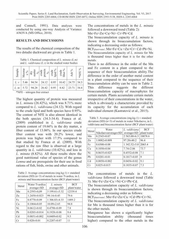
106
Scientific Papers. Series E. Land Reclamation, Earth Observation & Surveying, Environmental Engineering. Vol. VI, 2017Print ISSN 2285-6064, CD-ROM ISSN 2285-6072, Online ISSN 2393-5138, ISSN-L 2285-6064
and Connell, 1991). Data analyses were conducted by using one-way Analysis of Variance ANOVA (MS Office, 2010). RESULTS AND DISCUSSIONS The results of the chemical composition of the two dstudie duckweed are given in Table 1.
Table 1. Chemical composition of L. minuta (L.m) and L. valdiviana (L.v) in the studied water bodies
Sam
ple
Moi
stur
e %
dr
y m
atte
r %
cr
ude
prot
ein
%
crud
e lip
id %
crud
e fib
er %
Ash
%
*NFE
%
L. v 5.46 94.54 24.12 0.95 10.42 24.75 34.3
L. m 5.72 94.28 26.42 0.95 8.82 23.71 34.4 *NFE – nitrogen free extract The highest quantity of protein was measured in L. minuta (26.42%), which was 8.71% more compared to L. valdiviana (24.12). With regard to the crude lipid and both species have 0.95%. The content of NFE is also almost identical in the both species (34.3-34.4). Franca et al. (2009) established in L. valdiviana crude protein content of 19.66% in the dry matter, a fiber content of 13.06%. In our species crude fiber content was with 20.2% lower, and protein was higher with 17.5% compared to that studied by Franca et al. (2009). With regard to the raw fiber is observed at a large quantity in L. valdiviana (10.42%), and less in L. minuta (8.82%). All these results show the good nutritional value of species of the genus Lemna and are prerequisite for their use in food rations of fish, birds, swine and other animals.
Table 2. Average concentrations (mg.kg-1) ± standard deviation (SD) (n=3) of metals in water Tvardica, in L. minuta and bioconcentration factor (BCF plant/water)
Metal Water Tvardica average±SD
L. minuta average±SD
BCF plant/water
Mn 0.2593±0,09 3 199.61±5.32 12339.4 Zn 1.2450±0.023 99.14±0.45 79.6 Fe 0.8770±0.09 1 306.03±4.33 1489.2 Cu 0.1064±0.05 10.09±2.65 94.8 Ni 0.0612±0.02 0.4798±0.09 7.8 Pb 0.0203±0.014 0.1928±0.08 9.4 Cd 0.0051±0.002 0.0489±0.02 9.5 Cr 0.020±0.01 0.2207±0.07 11
The concentrations of metals in the L. minuta followed a downward trend (Table 2): Mn>Fe>Zn>Cu>Ni> Cr>Pb>Cd. The bioaccumulation capacity of L. minuta is shown through its bioaccumulation factors, indicating a decreasing order as follows: BCFplant/water: Mn>Fe>Cu >Zn>Cr> Cd>Pb>Ni. The bioaccumulation capacity of L. minuta for Mn is thousand times higher than it is for the other metals. There is no difference in the order of the Mn and Fe content in a plant compared to the sequence of their bioaccumulation ability.The difference in the order of another metal content in a plant compared to the sequence of their bioaccumulation ability can be seen in Table 2. This difference suggests the different bioaccumulation capacity of macrophytes for certain metals. Plants accumulate certain metals irrespective of their concentrations in the water, which is obviously a characteristic provided by its capacity for the accumulation of each individual element (Kastratović et al., 2015).
Table 3. Average concentrations (mg.kg-1) ± standard deviation (SD) (n=3) of metals in water Nikolaevo, in L. valdiviana and bioconcentration factor (BCF plant/water)
Metal Water Nikolaevoaverage±SD
L. valdiviana average±SD
BCF plant/water
Mn 0.2543±0.07 2 563.00±6.3 10078.6 Zn 1.0082±0.009 97.20±40.2 96.4 Fe 0.6500±0.08 1 342.52±5.0 2065.4 Cu 0.1050±0.04 7.74±2.06 73.7 Ni 0.0635±0.025 0.4552±0.08 7.1 Pb 0.0201±0.01 0.1817±0.05 9 Cd 0.0050±0.002 0.0456±0.02 9.1 Cr 0.025±0.015 0.1835±0.07 7.3 The concentrations of metals in the L. valdiviana followed a downward trend (Table 3): Mn>Fe>Zn>Cu >Ni>Cr>Pb>Cd. The bioaccumulation capacity of L. valdiviana is shown through its bioaccumulation factors, indicating a decreasing order as follows: BCFplant/water: Mn>Fe>Zn>Cu >Cd>Pb>Cr>Ni. The bioaccumulation capacity of L. valdiviana for Mn is thousand times higher than it is for the other metals. Manganese has shown a significantly higher bioaccumulation ability (thousand times higher) compared to the other metals in the
107
Scientific Papers. Series E. Land Reclamation, Earth Observation & Surveying, Environmental Engineering. Vol. VI, 2017Print ISSN 2285-6064, CD-ROM ISSN 2285-6072, Online ISSN 2393-5138, ISSN-L 2285-6064
and Connell, 1991). Data analyses were conducted by using one-way Analysis of Variance ANOVA (MS Office, 2010). RESULTS AND DISCUSSIONS The results of the chemical composition of the two dstudie duckweed are given in Table 1.
Table 1. Chemical composition of L. minuta (L.m) and L. valdiviana (L.v) in the studied water bodies
Sam
ple
Moi
stur
e %
dr
y m
atte
r %
cr
ude
prot
ein
%
crud
e lip
id %
crud
e fib
er %
Ash
%
*NFE
%
L. v 5.46 94.54 24.12 0.95 10.42 24.75 34.3
L. m 5.72 94.28 26.42 0.95 8.82 23.71 34.4 *NFE – nitrogen free extract The highest quantity of protein was measured in L. minuta (26.42%), which was 8.71% more compared to L. valdiviana (24.12). With regard to the crude lipid and both species have 0.95%. The content of NFE is also almost identical in the both species (34.3-34.4). Franca et al. (2009) established in L. valdiviana crude protein content of 19.66% in the dry matter, a fiber content of 13.06%. In our species crude fiber content was with 20.2% lower, and protein was higher with 17.5% compared to that studied by Franca et al. (2009). With regard to the raw fiber is observed at a large quantity in L. valdiviana (10.42%), and less in L. minuta (8.82%). All these results show the good nutritional value of species of the genus Lemna and are prerequisite for their use in food rations of fish, birds, swine and other animals.
Table 2. Average concentrations (mg.kg-1) ± standard deviation (SD) (n=3) of metals in water Tvardica, in L. minuta and bioconcentration factor (BCF plant/water)
Metal Water Tvardica average±SD
L. minuta average±SD
BCF plant/water
Mn 0.2593±0,09 3 199.61±5.32 12339.4 Zn 1.2450±0.023 99.14±0.45 79.6 Fe 0.8770±0.09 1 306.03±4.33 1489.2 Cu 0.1064±0.05 10.09±2.65 94.8 Ni 0.0612±0.02 0.4798±0.09 7.8 Pb 0.0203±0.014 0.1928±0.08 9.4 Cd 0.0051±0.002 0.0489±0.02 9.5 Cr 0.020±0.01 0.2207±0.07 11
The concentrations of metals in the L. minuta followed a downward trend (Table 2): Mn>Fe>Zn>Cu>Ni> Cr>Pb>Cd. The bioaccumulation capacity of L. minuta is shown through its bioaccumulation factors, indicating a decreasing order as follows: BCFplant/water: Mn>Fe>Cu >Zn>Cr> Cd>Pb>Ni. The bioaccumulation capacity of L. minuta for Mn is thousand times higher than it is for the other metals. There is no difference in the order of the Mn and Fe content in a plant compared to the sequence of their bioaccumulation ability.The difference in the order of another metal content in a plant compared to the sequence of their bioaccumulation ability can be seen in Table 2. This difference suggests the different bioaccumulation capacity of macrophytes for certain metals. Plants accumulate certain metals irrespective of their concentrations in the water, which is obviously a characteristic provided by its capacity for the accumulation of each individual element (Kastratović et al., 2015).
Table 3. Average concentrations (mg.kg-1) ± standard deviation (SD) (n=3) of metals in water Nikolaevo, in L. valdiviana and bioconcentration factor (BCF plant/water)
Metal Water Nikolaevoaverage±SD
L. valdiviana average±SD
BCF plant/water
Mn 0.2543±0.07 2 563.00±6.3 10078.6 Zn 1.0082±0.009 97.20±40.2 96.4 Fe 0.6500±0.08 1 342.52±5.0 2065.4 Cu 0.1050±0.04 7.74±2.06 73.7 Ni 0.0635±0.025 0.4552±0.08 7.1 Pb 0.0201±0.01 0.1817±0.05 9 Cd 0.0050±0.002 0.0456±0.02 9.1 Cr 0.025±0.015 0.1835±0.07 7.3 The concentrations of metals in the L. valdiviana followed a downward trend (Table 3): Mn>Fe>Zn>Cu >Ni>Cr>Pb>Cd. The bioaccumulation capacity of L. valdiviana is shown through its bioaccumulation factors, indicating a decreasing order as follows: BCFplant/water: Mn>Fe>Zn>Cu >Cd>Pb>Cr>Ni. The bioaccumulation capacity of L. valdiviana for Mn is thousand times higher than it is for the other metals. Manganese has shown a significantly higher bioaccumulation ability (thousand times higher) compared to the other metals in the
tissues of L. minuta and L. valdiviana. This established and Kastratović et al.(2015) inexamination to L. minor and recorded the average value of the content of Mn in the root 3427 mg.kg-1 and 2225 mg.kg-1 in leaves. In our both studied species the accumulation of heavy metals is comparable andwith the most strong bioaccumulation was observed in manganese and iron. These are metals which are necessary for the metabolism and can more easy to be absorbed from surrounding environment and transported to the green parts of the plants (Lasat, 2010). CONCLUSIONS In the studied L. minuta and L. valdiviana most accumulation of manganese was observed. Both species are with very good bioaccu-mulation of heavy metals and can be used for water treatment. Furthermore, it is found and a high content of protein in L. minuta and L. valdiviana (26.42% and 24.12%), which makes it possible to use as feed in nutrition different kinds of fish, poultry, swine and other animals. ACKNOWLEDGEMENTS This research work was carried out with the support of the Faculty of Agriculture, Trakia University, Project №2A/16. REFERENCES Abou el-Kheir W., Gahiza I., Farid A., Tarek T.,Doaa H.,
2007. Assessment of the Efficiency of Duckweed (Lemnagibba) in Wastewater Treatment. Interna-tional journal of agriculture & biology, 9 (5):681–687.
Chang J.S., Yoon H., Kim K., 2009. Heavy metal and arsenic accumulating fern species as potential ecological indicators in As-contaminated abandoned mines. Ecological Indicators, 9, 1275–1279.
Chaudhary E., Sharma P., 2014.Assessment of Heavy Metal Removal Efficiency of Lemna minor. International journal of innovative research and development, 3(6): 176-178.
Drost W., Matzke M,. Backhaus T., 2007. Heavy metal toxicity to Lemna minor: studies on the time dependence of growth inhibition and the recovery after exposure. Chemosphere, 67, 36-43.
Franca G., Filho J., Pereira G., Faria G., Melo F, Santos J., 2009.Valornutricional de Lemna valdiviana Phil (Araceae) submetida a diferentes concentration de
fertilization com excremento de aves. Biotemas, 22 (3): 19-26.
Greger M., 1999. Metal availability and bioconcentration in plants, in:M.N.V. Prasad, J. Hagemeyer (Eds.), Heavy Metal Stress inPlants — From Molecules to Ecosystems, Springer, Berlin, 1–27.
Hawker D., Connell D., 1991. An evaluation between bioconcentration factor and aqueous solubility. Chemosphere,23, 231-241.
Kastratović V., Jaćimović Z., Đurović D., Bigović M., Krivokapić S. 2015. Lemna minor L. as bioindicator of heavy metal pollutionin Skadar Lake (Montenegro). Kragujevac J. Sci.,37, 123-134.
Landolt E., Kandeler R., 1987. The family of Lemnaceae - a monographic study, Vol. 2: Phytochemistry, physiology, application and bibliography., Vol. 4 in Biosystematic investigations in the family of duckweeds (Lemnaceae). Geobotanischen Instutites der ETH, Stiftung Rubel, Zurich.
Lasat M.M., 2010. Phytoextraction of metals from contaminated soil: A review of plant/soil/metal interaction and assessment of pertinent agronomic issues. Journal of Hazardous Substance Research, 2, 1-25.
Lehman P., Silk W., Knight A., 1981. Protein and Nitrate Content of Lemna Sp. as a Function of Developmental Stage and Incubation Temperature. Plant Physiol., 68, 127-132.
Lemon G.D., Posluszny U., Husband B.C., 2001. Potential and realized rates of vegetative reproduction in Spirodelapolyrhiza, Lemna minor, and Wolffia borealis.Aquat Bot., 70 (1): 79–87. doi:10.1016/ S0304-3770(00)00131-5.
Olajire A., Altenburgerb R., Kqsterb E., Brack W., 2005. Chemical and ecotoxicological assessment of polycyclic aromatic hydrocarbon—contaminated sediments of the Niger Delta, Southern Nigeria.Sci Tot Environ, 340, 123–136.
Prasad M., Malec P., Waloszek A., Bojko M., Strzałka K., 2001. Physiological responses of Lemnatrisulca L. (duckweed) to cadmium and copper bioaccumulation. Plant Science, 161, 881–889. DOI: 10.1016/S0168-9452(01)00478-2.
Van Hoeck A.,Horemans N., Monsieurs P., Cao H., Vandenhove H.,Blust R,. 2015. The first draft genome of the aquatic model plant Lemna minor opens the route for future stress physiology research and biotechnological applications. Biotechnol Biofuels, 8, 188.
Vinodhini R., Narayanan M., 2009. The Impact of toxic heavy metals on the hematological parameters in common Carp (Cyprinuscarpio L.). Iran. J. Environ. Health. Sci. Eng., 6(1): 23-28.
Yadav S.K., Juwarkar A., Kumar G., Thawale P., Singh S., Chakrabarti T., 2009. Bioaccumulation and phyto-translocation of arsenic, chromium and zinc by Jatrophacurcas L.: Impact of dairy sludge and biofertilizer. Bioresource Technology, 100, 4616–4622.
Zhao J., Davis L., Verpoorte R., 2005.Elicitor signal transduction leading to production of plant secondary metabolites. Biotechnol. Adv., 23, 283–333.
108
Scientific Papers. Series E. Land Reclamation, Earth Observation & Surveying, Environmental Engineering. Vol. VI, 2017Print ISSN 2285-6064, CD-ROM ISSN 2285-6072, Online ISSN 2393-5138, ISSN-L 2285-6064
STUDY ON PHYSICO-CHEMICAL PROPERTIES OF SOIL
IN THE RADES MINE AREA
Mihaela Adriana BABAU, Valer MICLE, Ioana Monica SUR
Technical University of Cluj-Napoca, 103-105 Muncii Blvd., 400641 Cluj-Napoca, Romania
Corresponding author email: [email protected]
Abstract Past mining activities in the Almasu Mare area have led, along the time, to environmental pollution, especially of the soil. Rades gold mine is a source of negative impact today. The improperly mine closure gives the possibility of the leaks from the inside of mine to arrive at surface, creating large imbalances in soil and not only. Also, the sterile dump which is very near of Rades mine is a concern for the environment from Almasu Mare because it is not subject to ecological coating process, and the wind and rain can lead the particulates on the surface of the dump at long distances. In order to analyse the current situation of soil in Rades mine area some physico-chemical analysis were performed. The physico-chemical analysis consisted in determination of the humidity content, the structure, texture and pH of the soil. The results of experiments related to the humidity showed that the soil humidity in the forest (18.34%-34.77%) was higher than the humidity determined from the surface tailings of Rades dump (14.15% - 22.39%). The soil in forest area is partially structured and the dump material is poorly or very poorly structured. The dump material and soil texture is largely rough and the pH of tailings material taken from the Rades dump surface was in the range of 3.4-4.8 pH units and in the forest was in the range of 5.3-5.6 pH units. Key words: environment, mining activities, physico-chemical parameters, Rades mine, soil pollution INTRODUCTION The soil is defined as the surface layer of the earth's crust. Is made of mineral particles, organic matter, water, air and living organisms. It is very dynamic performs many functions and is vital to human activities and survival of ecosystems (Oh et al., 2013). Therefore, soil is the fundamental foundation of our agricultural resources, food security, global economy and environmental quality (Oh et al., 2014). Soil pollution is a problem worldwide, often resulting from the legacy of industrial activities, waste management practices, and mining activity (Gay and Korre, 2006) with a potential threat to human health (Vidali, 2001). Mining activities in recent decades, was lead to generation of huge quantities of mining waste. Their poor management in the past has resulted the accumulation of heavy metals in the environment which contributing to contamination of soil substrates, destroying its texture, green landscapes, groundwater pollution and decreased biodiversity (Liu et al., 2008). Non-ferrous mining activity (including the mining, transport and preparation) is a
source of soil pollution. When the ore is crushed, some heavy metals reach the earth's surface and these settle in soil and water due to air diffusion. Cadmium, chromium, copper, mercury, lead, nickel and zinc are metals that represent an effect of concern (Babut et al., 2012). Following activities performed in the past, in the underground mines, have been produced huge amounts of sterile that are brought to the soil surface. This often becomes toxic waste when in contact with air and water. Surface tailings particles arrive in the air by wind action and can be transported long distances then deposited on soil, contributing to its pollution. Romania has a long-standing tradition of mining, particularly within the Apuseni mountains area. Unfortunately, in this area there are various negative consequences which occur as a direct and indirect result of mining process, such as: acid mine drainage, heavy metal pollution and degradation of environmental and life quality (Dabu, 2015). Heavy metal pollution has a cumulative character. Once contaminated, soil can no longer be regenerated (only very difficult) and
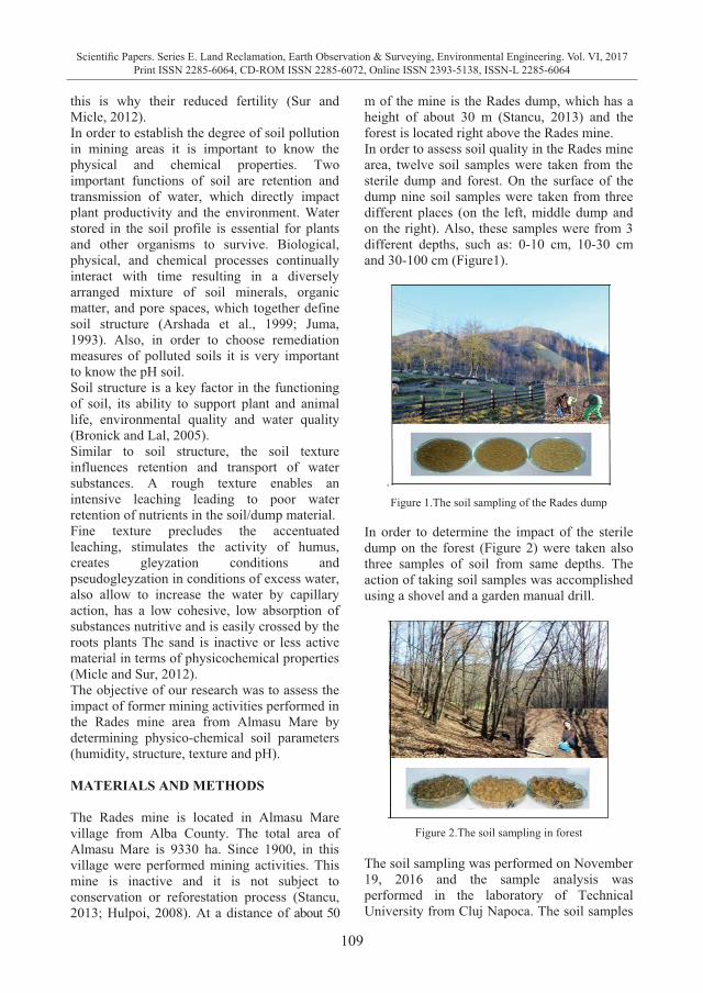
109
Scientific Papers. Series E. Land Reclamation, Earth Observation & Surveying, Environmental Engineering. Vol. VI, 2017Print ISSN 2285-6064, CD-ROM ISSN 2285-6072, Online ISSN 2393-5138, ISSN-L 2285-6064
STUDY ON PHYSICO-CHEMICAL PROPERTIES OF SOIL
IN THE RADES MINE AREA
Mihaela Adriana BABAU, Valer MICLE, Ioana Monica SUR
Technical University of Cluj-Napoca, 103-105 Muncii Blvd., 400641 Cluj-Napoca, Romania
Corresponding author email: [email protected]
Abstract Past mining activities in the Almasu Mare area have led, along the time, to environmental pollution, especially of the soil. Rades gold mine is a source of negative impact today. The improperly mine closure gives the possibility of the leaks from the inside of mine to arrive at surface, creating large imbalances in soil and not only. Also, the sterile dump which is very near of Rades mine is a concern for the environment from Almasu Mare because it is not subject to ecological coating process, and the wind and rain can lead the particulates on the surface of the dump at long distances. In order to analyse the current situation of soil in Rades mine area some physico-chemical analysis were performed. The physico-chemical analysis consisted in determination of the humidity content, the structure, texture and pH of the soil. The results of experiments related to the humidity showed that the soil humidity in the forest (18.34%-34.77%) was higher than the humidity determined from the surface tailings of Rades dump (14.15% - 22.39%). The soil in forest area is partially structured and the dump material is poorly or very poorly structured. The dump material and soil texture is largely rough and the pH of tailings material taken from the Rades dump surface was in the range of 3.4-4.8 pH units and in the forest was in the range of 5.3-5.6 pH units. Key words: environment, mining activities, physico-chemical parameters, Rades mine, soil pollution INTRODUCTION The soil is defined as the surface layer of the earth's crust. Is made of mineral particles, organic matter, water, air and living organisms. It is very dynamic performs many functions and is vital to human activities and survival of ecosystems (Oh et al., 2013). Therefore, soil is the fundamental foundation of our agricultural resources, food security, global economy and environmental quality (Oh et al., 2014). Soil pollution is a problem worldwide, often resulting from the legacy of industrial activities, waste management practices, and mining activity (Gay and Korre, 2006) with a potential threat to human health (Vidali, 2001). Mining activities in recent decades, was lead to generation of huge quantities of mining waste. Their poor management in the past has resulted the accumulation of heavy metals in the environment which contributing to contamination of soil substrates, destroying its texture, green landscapes, groundwater pollution and decreased biodiversity (Liu et al., 2008). Non-ferrous mining activity (including the mining, transport and preparation) is a
source of soil pollution. When the ore is crushed, some heavy metals reach the earth's surface and these settle in soil and water due to air diffusion. Cadmium, chromium, copper, mercury, lead, nickel and zinc are metals that represent an effect of concern (Babut et al., 2012). Following activities performed in the past, in the underground mines, have been produced huge amounts of sterile that are brought to the soil surface. This often becomes toxic waste when in contact with air and water. Surface tailings particles arrive in the air by wind action and can be transported long distances then deposited on soil, contributing to its pollution. Romania has a long-standing tradition of mining, particularly within the Apuseni mountains area. Unfortunately, in this area there are various negative consequences which occur as a direct and indirect result of mining process, such as: acid mine drainage, heavy metal pollution and degradation of environmental and life quality (Dabu, 2015). Heavy metal pollution has a cumulative character. Once contaminated, soil can no longer be regenerated (only very difficult) and
this is why their reduced fertility (Sur and Micle, 2012). In order to establish the degree of soil pollution in mining areas it is important to know the physical and chemical properties. Two important functions of soil are retention and transmission of water, which directly impact plant productivity and the environment. Water stored in the soil profile is essential for plants and other organisms to survive. Biological, physical, and chemical processes continually interact with time resulting in a diversely arranged mixture of soil minerals, organic matter, and pore spaces, which together define soil structure (Arshada et al., 1999; Juma, 1993). Also, in order to choose remediation measures of polluted soils it is very important to know the pH soil. Soil structure is a key factor in the functioning of soil, its ability to support plant and animal life, environmental quality and water quality (Bronick and Lal, 2005). Similar to soil structure, the soil texture influences retention and transport of water substances. A rough texture enables an intensive leaching leading to poor water retention of nutrients in the soil/dump material. Fine texture precludes the accentuated leaching, stimulates the activity of humus, creates gleyzation conditions and pseudogleyzation in conditions of excess water, also allow to increase the water by capillary action, has a low cohesive, low absorption of substances nutritive and is easily crossed by the roots plants The sand is inactive or less active material in terms of physicochemical properties (Micle and Sur, 2012). The objective of our research was to assess the impact of former mining activities performed in the Rades mine area from Almasu Mare by determining physico-chemical soil parameters (humidity, structure, texture and pH). MATERIALS AND METHODS The Rades mine is located in Almasu Mare village from Alba County. The total area of Almasu Mare is 9330 ha. Since 1900, in this village were performed mining activities. This mine is inactive and it is not subject to conservation or reforestation process (Stancu, 2013; Hulpoi, 2008). At a distance of about 50
m of the mine is the Rades dump, which has a height of about 30 m (Stancu, 2013) and the forest is located right above the Rades mine. In order to assess soil quality in the Rades mine area, twelve soil samples were taken from the sterile dump and forest. On the surface of the dump nine soil samples were taken from three different places (on the left, middle dump and on the right). Also, these samples were from 3 different depths, such as: 0-10 cm, 10-30 cm and 30-100 cm (Figure1).
. Figure 1.The soil sampling of the Rades dump
In order to determine the impact of the sterile dump on the forest (Figure 2) were taken also three samples of soil from same depths. The action of taking soil samples was accomplished using a shovel and a garden manual drill.
Figure 2.The soil sampling in forest
The soil sampling was performed on November 19, 2016 and the sample analysis was performed in the laboratory of Technical University from Cluj Napoca. The soil samples
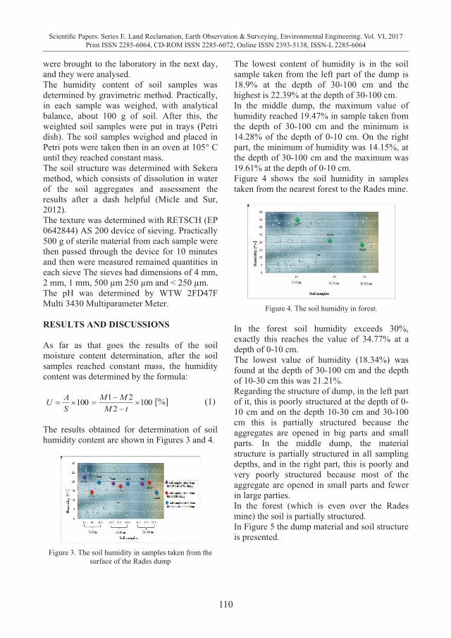
110
Scientific Papers. Series E. Land Reclamation, Earth Observation & Surveying, Environmental Engineering. Vol. VI, 2017Print ISSN 2285-6064, CD-ROM ISSN 2285-6072, Online ISSN 2393-5138, ISSN-L 2285-6064
were brought to the laboratory in the next day, and they were analysed. The humidity content of soil samples was determined by gravimetric method. Practically, in each sample was weighed, with analytical balance, about 100 g of soil. After this, the weighted soil samples were put in trays (Petri dish). The soil samples weighed and placed in Petri pots were taken then in an oven at 105° C until they reached constant mass. The soil structure was determined with Sekera method, which consists of dissolution in water of the soil aggregates and assessment the results after a dash helpful (Micle and Sur, 2012). The texture was determined with RETSCH (EP 0642844) AS 200 device of sieving. Practically 500 g of sterile material from each sample were then passed through the device for 10 minutes and then were measured remained quantities in each sieve The sieves had dimensions of 4 mm, 2 mm, 1 mm, 500 µm 250 µm and < 250 µm. The pH was determined by WTW 2FD47F Multi 3430 Multiparameter Meter. RESULTS AND DISCUSSIONS As far as that goes the results of the soil moisture content determination, after the soil samples reached constant mass, the humidity content was determined by the formula:
1002
21100 ��
����
tMMM
SAU [%] (1)
The results obtained for determination of soil humidity content are shown in Figures 3 and 4.
Figure 3. The soil humidity in samples taken from the
surface of the Rades dump
The lowest content of humidity is in the soil sample taken from the left part of the dump is 18.9% at the depth of 30-100 cm and the highest is 22.39% at the depth of 30-100 cm. In the middle dump, the maximum value of humidity reached 19.47% in sample taken from the depth of 30-100 cm and the minimum is 14.28% of the depth of 0-10 cm. On the right part, the minimum of humidity was 14.15%, at the depth of 30-100 cm and the maximum was 19.61% at the depth of 0-10 cm. Figure 4 shows the soil humidity in samples taken from the nearest forest to the Rades mine.
Figure 4. The soil humidity in forest.
In the forest soil humidity exceeds 30%, exactly this reaches the value of 34.77% at a depth of 0-10 cm. The lowest value of humidity (18.34%) was found at the depth of 30-100 cm and the depth of 10-30 cm this was 21.21%. Regarding the structure of dump, in the left part of it, this is poorly structured at the depth of 0-10 cm and on the depth 10-30 cm and 30-100 cm this is partially structured because the aggregates are opened in big parts and small parts. In the middle dump, the material structure is partially structured in all sampling depths, and in the right part, this is poorly and very poorly structured because most of the aggregate are opened in small parts and fewer in large parties. In the forest (which is even over the Rades mine) the soil is partially structured. In Figure 5 the dump material and soil structure is presented.
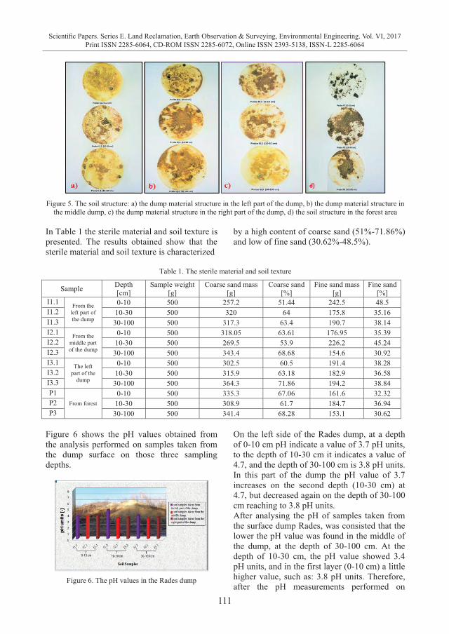
111
Scientific Papers. Series E. Land Reclamation, Earth Observation & Surveying, Environmental Engineering. Vol. VI, 2017Print ISSN 2285-6064, CD-ROM ISSN 2285-6072, Online ISSN 2393-5138, ISSN-L 2285-6064
were brought to the laboratory in the next day, and they were analysed. The humidity content of soil samples was determined by gravimetric method. Practically, in each sample was weighed, with analytical balance, about 100 g of soil. After this, the weighted soil samples were put in trays (Petri dish). The soil samples weighed and placed in Petri pots were taken then in an oven at 105° C until they reached constant mass. The soil structure was determined with Sekera method, which consists of dissolution in water of the soil aggregates and assessment the results after a dash helpful (Micle and Sur, 2012). The texture was determined with RETSCH (EP 0642844) AS 200 device of sieving. Practically 500 g of sterile material from each sample were then passed through the device for 10 minutes and then were measured remained quantities in each sieve The sieves had dimensions of 4 mm, 2 mm, 1 mm, 500 µm 250 µm and < 250 µm. The pH was determined by WTW 2FD47F Multi 3430 Multiparameter Meter. RESULTS AND DISCUSSIONS As far as that goes the results of the soil moisture content determination, after the soil samples reached constant mass, the humidity content was determined by the formula:
1002
21100 ��
����
tMMM
SAU [%] (1)
The results obtained for determination of soil humidity content are shown in Figures 3 and 4.
Figure 3. The soil humidity in samples taken from the
surface of the Rades dump
The lowest content of humidity is in the soil sample taken from the left part of the dump is 18.9% at the depth of 30-100 cm and the highest is 22.39% at the depth of 30-100 cm. In the middle dump, the maximum value of humidity reached 19.47% in sample taken from the depth of 30-100 cm and the minimum is 14.28% of the depth of 0-10 cm. On the right part, the minimum of humidity was 14.15%, at the depth of 30-100 cm and the maximum was 19.61% at the depth of 0-10 cm. Figure 4 shows the soil humidity in samples taken from the nearest forest to the Rades mine.
Figure 4. The soil humidity in forest.
In the forest soil humidity exceeds 30%, exactly this reaches the value of 34.77% at a depth of 0-10 cm. The lowest value of humidity (18.34%) was found at the depth of 30-100 cm and the depth of 10-30 cm this was 21.21%. Regarding the structure of dump, in the left part of it, this is poorly structured at the depth of 0-10 cm and on the depth 10-30 cm and 30-100 cm this is partially structured because the aggregates are opened in big parts and small parts. In the middle dump, the material structure is partially structured in all sampling depths, and in the right part, this is poorly and very poorly structured because most of the aggregate are opened in small parts and fewer in large parties. In the forest (which is even over the Rades mine) the soil is partially structured. In Figure 5 the dump material and soil structure is presented.
Figure 5. The soil structure: a) the dump material structure in the left part of the dump, b) the dump material structure in
the middle dump, c) the dump material structure in the right part of the dump, d) the soil structure in the forest area In Table 1 the sterile material and soil texture is presented. The results obtained show that the sterile material and soil texture is characterized
by a high content of coarse sand (51%-71.86%) and low of fine sand (30.62%-48.5%).
Table 1. The sterile material and soil texture
Sample Depth [cm]
Sample weight [g]
Coarse sand mass [g]
Coarse sand [%]
Fine sand mass [g]
Fine sand [%]
I1.1 From the left part of the dump
0-10 500 257.2 51.44 242.5 48.5 I1.2 10-30 500 320 64 175.8 35.16 I1.3 30-100 500 317.3 63.4 190.7 38.14 I2.1 From the
middle part of the dump
0-10 500 318.05 63.61 176.95 35.39 I2.2 10-30 500 269.5 53.9 226.2 45.24 I2.3 30-100 500 343.4 68.68 154.6 30.92 I3.1 The left
part of the dump
0-10 500 302.5 60.5 191.4 38.28 I3.2 10-30 500 315.9 63.18 182.9 36.58 I3.3 30-100 500 364.3 71.86 194.2 38.84 P1
From forest 0-10 500 335.3 67.06 161.6 32.32
P2 10-30 500 308.9 61.7 184.7 36.94 P3 30-100 500 341.4 68.28 153.1 30.62
Figure 6 shows the pH values obtained from the analysis performed on samples taken from the dump surface on those three sampling depths.
Figure 6. The pH values in the Rades dump
On the left side of the Rades dump, at a depth of 0-10 cm pH indicate a value of 3.7 pH units, to the depth of 10-30 cm it indicates a value of 4.7, and the depth of 30-100 cm is 3.8 pH units. In this part of the dump the pH value of 3.7 increases on the second depth (10-30 cm) at 4.7, but decreased again on the depth of 30-100 cm reaching to 3.8 pH units. After analysing the pH of samples taken from the surface dump Rades, was consisted that the lower the pH value was found in the middle of the dump, at the depth of 30-100 cm. At the depth of 10-30 cm, the pH value showed 3.4 pH units, and in the first layer (0-10 cm) a little higher value, such as: 3.8 pH units. Therefore, after the pH measurements performed on
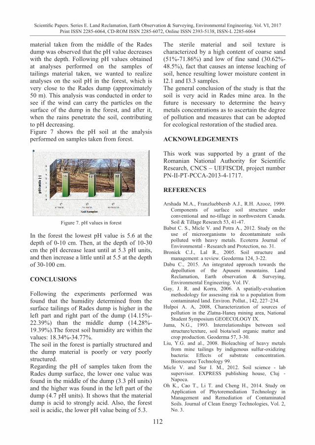
112
Scientific Papers. Series E. Land Reclamation, Earth Observation & Surveying, Environmental Engineering. Vol. VI, 2017Print ISSN 2285-6064, CD-ROM ISSN 2285-6072, Online ISSN 2393-5138, ISSN-L 2285-6064
material taken from the middle of the Rades dump was observed that the pH value decreases with the depth. Following pH values obtained at analyses performed on the samples of tailings material taken, we wanted to realize analyses on the soil pH in the forest, which is very close to the Rades dump (approximately 50 m). This analysis was conducted in order to see if the wind can carry the particles on the surface of the dump in the forest, and after it, when the rains penetrate the soil, contributing to pH decreasing. Figure 7 shows the pH soil at the analysis performed on samples taken from forest.
Figure 7. pH values in forest
In the forest the lowest pH value is 5.6 at the depth of 0-10 cm. Then, at the depth of 10-30 cm the pH decrease least until at 5.3 pH units, and then increase a little until at 5.5 at the depth of 30-100 cm. CONCLUSIONS Following the experiments performed was found that the humidity determined from the surface tailings of Rades dump is higher in the left part and right part of the dump (14.15%-22.39%) than the middle dump (14.28%-19.39%).The forest soil humidity are within the values: 18.34%-34.77%. The soil in the forest is partially structured and the dump material is poorly or very poorly structured. Regarding the pH of samples taken from the Rades dump surface, the lower one value was found in the middle of the dump (3.3 pH units) and the higher was found in the left part of the dump (4.7 pH units). It shows that the material dump is acid to strongly acid. Also, the forest soil is acidic, the lower pH value being of 5.3.
The sterile material and soil texture is characterized by a high content of coarse sand (51%-71.86%) and low of fine sand (30.62%-48.5%), fact that causes an intense leaching of soil, hence resulting lower moisture content in I2.1 and I3.3 samples. The general conclusion of the study is that the soil is very acid in Rades mine area. In the future is necessary to determine the heavy metals concentrations as to ascertain the degree of pollution and measures that can be adopted for ecological restoration of the studied area. ACKNOWLEDGEMENTS This work was supported by a grant of the Romanian National Authority for Scientific Research, CNCS – UEFISCDI, project number PN-II-PT-PCCA-2013-4-1717. REFERENCES Arshada M.A., Franzluebbersb A.J., R.H. Azooz, 1999.
Components of surface soil structure under conventional and no-tillage in northwestern Canada. Soil & Tillage Research 53, 41-47.
Babut C. S., Micle V. and Potra A., 2012. Study on the use of microorganisms to decontaminate soils polluted with heavy metals. Ecoterra Journal of Environmental - Research and Protection, no. 31.
Bronick C.J., Lal R., 2005. Soil structure and management: a review. Geoderma 124, 3-22.
Dabu C., 2015. An integrated approach towards the depollution of the Apuseni mountains. Land Reclamation, Earth observation & Surveying, Environmental Engineering. Vol. IV.
Gay, J. R. and Korra, 2006. A spatially-evaluation methodology for assessing risk to a population from contaminated land. Environ. Pollut., 142, 227–234.
Hulpoi A. A, 2008, Characterization of sources of pollution in the Zlatna-Haneş mining area, National Student Symposium GEOECOLOGY IX.
Juma, N.G., 1993. Interrelationships between soil structure/texture, soil biota/soil organic matter and crop production. Geoderma 57, 3-30.
Liu, Y.G. and al., 2008. Bioleaching of heavy metals from mine tailings by indigenous sulfur-oxidizing bacteria: Effects of substrate concentration. Bioresource Technology 99.
Micle V. and Sur I. M., 2012. Soil science - lab supervisor. EXPRESS publishing house, Cluj - Napoca.
Oh K., Cao T., Li T. and Cheng H., 2014. Study on Application of Phytoremediation Technology in Management and Remediation of Contaminated Soils. Journal of Clean Energy Technologies, Vol. 2, No. 3.

113
Scientific Papers. Series E. Land Reclamation, Earth Observation & Surveying, Environmental Engineering. Vol. VI, 2017Print ISSN 2285-6064, CD-ROM ISSN 2285-6072, Online ISSN 2393-5138, ISSN-L 2285-6064
material taken from the middle of the Rades dump was observed that the pH value decreases with the depth. Following pH values obtained at analyses performed on the samples of tailings material taken, we wanted to realize analyses on the soil pH in the forest, which is very close to the Rades dump (approximately 50 m). This analysis was conducted in order to see if the wind can carry the particles on the surface of the dump in the forest, and after it, when the rains penetrate the soil, contributing to pH decreasing. Figure 7 shows the pH soil at the analysis performed on samples taken from forest.
Figure 7. pH values in forest
In the forest the lowest pH value is 5.6 at the depth of 0-10 cm. Then, at the depth of 10-30 cm the pH decrease least until at 5.3 pH units, and then increase a little until at 5.5 at the depth of 30-100 cm. CONCLUSIONS Following the experiments performed was found that the humidity determined from the surface tailings of Rades dump is higher in the left part and right part of the dump (14.15%-22.39%) than the middle dump (14.28%-19.39%).The forest soil humidity are within the values: 18.34%-34.77%. The soil in the forest is partially structured and the dump material is poorly or very poorly structured. Regarding the pH of samples taken from the Rades dump surface, the lower one value was found in the middle of the dump (3.3 pH units) and the higher was found in the left part of the dump (4.7 pH units). It shows that the material dump is acid to strongly acid. Also, the forest soil is acidic, the lower pH value being of 5.3.
The sterile material and soil texture is characterized by a high content of coarse sand (51%-71.86%) and low of fine sand (30.62%-48.5%), fact that causes an intense leaching of soil, hence resulting lower moisture content in I2.1 and I3.3 samples. The general conclusion of the study is that the soil is very acid in Rades mine area. In the future is necessary to determine the heavy metals concentrations as to ascertain the degree of pollution and measures that can be adopted for ecological restoration of the studied area. ACKNOWLEDGEMENTS This work was supported by a grant of the Romanian National Authority for Scientific Research, CNCS – UEFISCDI, project number PN-II-PT-PCCA-2013-4-1717. REFERENCES Arshada M.A., Franzluebbersb A.J., R.H. Azooz, 1999.
Components of surface soil structure under conventional and no-tillage in northwestern Canada. Soil & Tillage Research 53, 41-47.
Babut C. S., Micle V. and Potra A., 2012. Study on the use of microorganisms to decontaminate soils polluted with heavy metals. Ecoterra Journal of Environmental - Research and Protection, no. 31.
Bronick C.J., Lal R., 2005. Soil structure and management: a review. Geoderma 124, 3-22.
Dabu C., 2015. An integrated approach towards the depollution of the Apuseni mountains. Land Reclamation, Earth observation & Surveying, Environmental Engineering. Vol. IV.
Gay, J. R. and Korra, 2006. A spatially-evaluation methodology for assessing risk to a population from contaminated land. Environ. Pollut., 142, 227–234.
Hulpoi A. A, 2008, Characterization of sources of pollution in the Zlatna-Haneş mining area, National Student Symposium GEOECOLOGY IX.
Juma, N.G., 1993. Interrelationships between soil structure/texture, soil biota/soil organic matter and crop production. Geoderma 57, 3-30.
Liu, Y.G. and al., 2008. Bioleaching of heavy metals from mine tailings by indigenous sulfur-oxidizing bacteria: Effects of substrate concentration. Bioresource Technology 99.
Micle V. and Sur I. M., 2012. Soil science - lab supervisor. EXPRESS publishing house, Cluj - Napoca.
Oh K., Cao T., Li T. and Cheng H., 2014. Study on Application of Phytoremediation Technology in Management and Remediation of Contaminated Soils. Journal of Clean Energy Technologies, Vol. 2, No. 3.
Oh K., Li T., Cheng H. Y., Xie Y. and Yonemochi S.,
2013. Development of Profitable Phytoremediation of Contaminated Soils with Biofuel Crops. Journal of Environmental Protection, vol. 4, pp. 58-64.
Sur I.M. and Micle V., 2012. Zinc and copper extraction in soils polluted by biolixiviere in situ. Environmental Engineering and Sustainable Development Entrepreneurship - Vol. 1, No. 53, 49.51.
Stancu P.T., 2013. PhD thesis entitled: "Studies geochemical and mineralogical changes resulting from secondary processes of mining and remediation technologies areas polluted with heavy metals and/or rare in the Zlatna, Faculty of Geology and Geophysics, Bucharest.
Vidali, M., 2001. Bioremediation - An overview. Pure Appl. Chem., 73, 1163–1172.
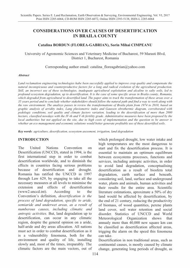
114
Scientific Papers. Series E. Land Reclamation, Earth Observation & Surveying, Environmental Engineering. Vol. VI, 2017Print ISSN 2285-6064, CD-ROM ISSN 2285-6072, Online ISSN 2393-5138, ISSN-L 2285-6064
CONSIDERATIONS OVER CAUSES OF DESERTIFICATION
IN BRAILA COUNTY
Catalina BORDUN (FLOREA-GABRIAN), Sorin Mihai CIMPEANU
University of Agronomic Sciences and Veterinary Medicine of Bucharest, 59 Marasti Blvd, District 1, Bucharest, Romania
Corresponding author email: [email protected]
Abstract Land reclamation engineering technologies habe been succesfully applied to improve crop quality and compensate the natural inconspicuous and counterproductive factors for a long and radical evolution of the agricultural production. Still, an incorrect use of these technologies, inadequate agricultural exploitation and alcaline to salty soils, led to profound ecosystem degradation, up to desertification. It is the case of some specific areas in Braila county, Romania, which degraded from agricultural to desertified land. The paper aims to track the transformation of these areas over a 35 years period and to conclude whether stakeholders should follow the natural path and find a way to work along with the raw environment. The analisys passes in review the transformations of Braila plain from 1974 to 2010, based on graphic analysis of arridity index, Lang pluviometric index and Gaussen obrothermic diagram, corroborated with pedologic conditions, soil quality and climate factors variation, leading to the desertification of more than 2000 hectars, classified nowdays with the IV-th and V-th fertility grade. Administrative measures have been proposed by the local authorities but not applied on the site, due to high costs of implementation and the question to be answer is whether an eco management and economic solutions would better generate profitable use of these desertified soils. Key words: agriculture, desertfication, ecosystem asessment, irrigation, land degradation INTRODUCTION The United Nations Convention on Desertification (UNCCD), stated in 1994, is the first international step in order to combat desertification worldwide, and to diminish the effects in countries facing serious problems because of desertification and drought. Romania has ratified the UNCCD in 1997 through Law 629, by engaging to take all the necessary measures at all levels to minimise the extension and effects of desertification (www2.unccd.int). According to the Convention’s definition, desertification is the process of land degradation, specific to aride, semiaride and underwet areas, as a result of numberous causes, including climatic and antropic activities. But, land degradation up to desertification, can occur in any climatic region, despite the general opinion on a aride, half-aride and dry areas allocation. All nations must act in order to combat desertification as it is a vulnerability fenomena, both for the environment and quality of life, installing slowly and, most of the times, irreparably. The climatic factors are the main vectors, out of
which prelonged drought, low water intake and high temperatures are the most dangerous to start and fix the desertification process. It is essential to maintain an optimum equilibrum between ecosystems processes, functions and services, including antropic activities, in order to avoid land degradation, conceptualising desertification as a result of biosfera total degradation, earth surface and beneath, considering soil, land, surface and underground water, plants and animals, human activities and their results for the entire area. Scientific literature estimations, aproximate a 50% of dry land would be affected by desertification, by the end of 21 century, reducing the productivity of biomass, of wood quantities, perene plants land cover, soil water retention and social disorder. Statistics of UNCCD and World Meteorological Organization shows that annualy more than 40,000 new square km can be classified as desertification affected areas, trigging the alarm on the speed this fenomena can take. Desertification in non traditional areas, such as continental causes, is mostly caused by climate change, generating long periods of drought, as
115
Scientific Papers. Series E. Land Reclamation, Earth Observation & Surveying, Environmental Engineering. Vol. VI, 2017Print ISSN 2285-6064, CD-ROM ISSN 2285-6072, Online ISSN 2393-5138, ISSN-L 2285-6064
CONSIDERATIONS OVER CAUSES OF DESERTIFICATION
IN BRAILA COUNTY
Catalina BORDUN (FLOREA-GABRIAN), Sorin Mihai CIMPEANU
University of Agronomic Sciences and Veterinary Medicine of Bucharest, 59 Marasti Blvd, District 1, Bucharest, Romania
Corresponding author email: [email protected]
Abstract Land reclamation engineering technologies habe been succesfully applied to improve crop quality and compensate the natural inconspicuous and counterproductive factors for a long and radical evolution of the agricultural production. Still, an incorrect use of these technologies, inadequate agricultural exploitation and alcaline to salty soils, led to profound ecosystem degradation, up to desertification. It is the case of some specific areas in Braila county, Romania, which degraded from agricultural to desertified land. The paper aims to track the transformation of these areas over a 35 years period and to conclude whether stakeholders should follow the natural path and find a way to work along with the raw environment. The analisys passes in review the transformations of Braila plain from 1974 to 2010, based on graphic analysis of arridity index, Lang pluviometric index and Gaussen obrothermic diagram, corroborated with pedologic conditions, soil quality and climate factors variation, leading to the desertification of more than 2000 hectars, classified nowdays with the IV-th and V-th fertility grade. Administrative measures have been proposed by the local authorities but not applied on the site, due to high costs of implementation and the question to be answer is whether an eco management and economic solutions would better generate profitable use of these desertified soils. Key words: agriculture, desertfication, ecosystem asessment, irrigation, land degradation INTRODUCTION The United Nations Convention on Desertification (UNCCD), stated in 1994, is the first international step in order to combat desertification worldwide, and to diminish the effects in countries facing serious problems because of desertification and drought. Romania has ratified the UNCCD in 1997 through Law 629, by engaging to take all the necessary measures at all levels to minimise the extension and effects of desertification (www2.unccd.int). According to the Convention’s definition, desertification is the process of land degradation, specific to aride, semiaride and underwet areas, as a result of numberous causes, including climatic and antropic activities. But, land degradation up to desertification, can occur in any climatic region, despite the general opinion on a aride, half-aride and dry areas allocation. All nations must act in order to combat desertification as it is a vulnerability fenomena, both for the environment and quality of life, installing slowly and, most of the times, irreparably. The climatic factors are the main vectors, out of
which prelonged drought, low water intake and high temperatures are the most dangerous to start and fix the desertification process. It is essential to maintain an optimum equilibrum between ecosystems processes, functions and services, including antropic activities, in order to avoid land degradation, conceptualising desertification as a result of biosfera total degradation, earth surface and beneath, considering soil, land, surface and underground water, plants and animals, human activities and their results for the entire area. Scientific literature estimations, aproximate a 50% of dry land would be affected by desertification, by the end of 21 century, reducing the productivity of biomass, of wood quantities, perene plants land cover, soil water retention and social disorder. Statistics of UNCCD and World Meteorological Organization shows that annualy more than 40,000 new square km can be classified as desertification affected areas, trigging the alarm on the speed this fenomena can take. Desertification in non traditional areas, such as continental causes, is mostly caused by climate change, generating long periods of drought, as
dual fenomena acting biophisically and antropically and interacting in the eco-social systems of all worldwide populations (Reed and Stringer, 2016). Worldwide more than 100 countries facing the desertification problem; combinating processes such as wing and hidro erosion, vegetation devastation, land cover diminish, unrationalised water consume, soil salinisation, are agregate intensified by antropic activities, generating desertification and speeding up the process, in some regions. Scientific and organisational international comunities consider desertification as a major environmental issue and evenly an antropic disaster, placing desertification the third, after climate change and fresh water diminishing sources, in a classification of most important concerns of the 21st century. In Romania, a traditionally continental country, out of the total agricultural land, about 1/3 is affected by different stages of degradation, the most important triggering factors being water erosion and landslide, affecting 7 million ha (http://www.unccd.int/ActionProgrammes/ romania-eng2000.pdf). In order to minimise and reduce the effects of climate change and antropic actions, generating desertification in vulnerable areas, Romaia is implementing the National Strategy for Drought Effects Reduction, Prevention and Control of Land Degradation and Desertification, for Short, Medium and Long Terms, elaborated in 2000 and updated in 2008. The main objectives of the Strategy is to indicate and implement actions for short, medium and long term in order to reduce the vulnerability of local communities, natural ecosistems and socio-economic activities and to diminish their impact and effect over social order, local economies and natural environment (http://old.madr.ro/pages/strategie/strategie_antiseceta_update_09.05.2008.pdf). The affected areas in Romania are Moldova plateau, sub-Carpathian hills between Trotus and Olt rivers, Transylvanian plateau and Getic Piedmont, where estimations are of annual 123 tons of soil losses due to erosion. Climatic indexes for the last 35 years indicate that Romania’s climate has a high tendency to arid, influencing and intensifying the pedologic resources degradation up to desertification,
mostly in the dry areas of the country. Over the years, Romania has had a numerous drought intervals, which favorited the desertification of vulnerable areas, such as:
- First interval, between 1894–1905, with pick of the drought in 1897;
- Second interval, between 1942–1953, where 1944 was an extremly drought afflicted year (Ionescu-Sisesti Gh., 1946);
- Third interval, from 1992–2000, considered the first and last years as the most dried ones;
- Fourth interval, from 2006 to 2008, with 2007 as benchmark for high temperatures, the winter of this year being the mildest in the history of meteorological registry in Romania.
The considerations to establish the drought intervals, relay on at least 14 consecutive days in the cold season (December to March) and at least 10 consecutive days in the warm season (April to September), with no precipitation or, with quantities of less than 0,1 mm/day (Bogdan, 1981). Braila county is situated in the south est of Romania, as part of the Romanian Plain, with a total area of 4765.8 square km. Despite the general plain aspect, the relief is quite diverse, with numerous hillocks and hollows, sand dunes, largi river junctions, meanders and patchs. The most important hydrological artery is the Danube, along with the rivers: Siret, for only 50 km, Buzau for 126 km and Calmatui for 84 km; the hydrological network si completed by lakes, Ianca with 332 hectares, Plopu with 300 hectares and Lutul Alb with 357 hectares, formed in loess or cenote, floatable lough, such as Jirlau with 1086 hectares, Caineni with 74 hectares and Ciulnita with 92 hectares, functioning as natural compensation pond; also, due to a high concentration of salt, some of the lakes in the county have been clasified as balneo climateric resort, such as Lacu Sarat - Braila, Sarat Batogu, Tataru-Caineni and Movila Miresii, whith therapeutic properties. The total arabil area is of 395,870 hectars, out of which only 20,652 hectars of forests, meaning less than 4% which places the county on a dangerous low level, compared to the 28% average in Romania or 35% in Europe. Without the forestration protection and corroborated with the antropic and natural
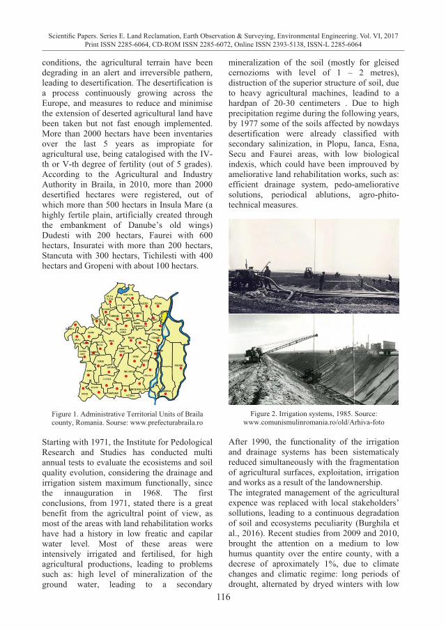
116
Scientific Papers. Series E. Land Reclamation, Earth Observation & Surveying, Environmental Engineering. Vol. VI, 2017Print ISSN 2285-6064, CD-ROM ISSN 2285-6072, Online ISSN 2393-5138, ISSN-L 2285-6064
conditions, the agricultural terrain have been degrading in an alert and irreversible pathern, leading to desertification. The desertification is a process continuously growing across the Europe, and measures to reduce and minimise the extension of deserted agricultural land have been taken but not fast enough implemented. More than 2000 hectars have been inventaries over the last 5 years as impropiate for agricultural use, being catalogised with the IV-th or V-th degree of fertility (out of 5 grades). According to the Agricultural and Industry Authority in Braila, in 2010, more than 2000 desertified hectares were registered, out of which more than 500 hectars in Insula Mare (a highly fertile plain, artificially created through the embankment of Danube’s old wings) Dudesti with 200 hectars, Faurei with 600 hectars, Insuratei with more than 200 hectars, Stancuta with 300 hectars, Tichilesti with 400 hectars and Gropeni with about 100 hectars.
Figure 1. Administrative Territorial Units of Braila county, Romania. Sourse: www.prefecturabraila.ro
Starting with 1971, the Institute for Pedological Research and Studies has conducted multi annual tests to evaluate the ecosistems and soil quality evolution, considering the drainage and irrigation sistem maximum functionally, since the innauguration in 1968. The first conclusions, from 1971, stated there is a great benefit from the agricultral point of view, as most of the areas with land rehabilitation works have had a history in low freatic and capilar water level. Most of these areas were intensively irrigated and fertilised, for high agricultural productions, leading to problems such as: high level of mineralization of the ground water, leading to a secondary
mineralization of the soil (mostly for gleised cernozioms with level of 1 – 2 metres), distruction of the superior structure of soil, due to heavy agricultural machines, leadind to a hardpan of 20-30 centimeters . Due to high precipitation regime during the following years, by 1977 some of the soils affected by nowdays desertification were already classified with secondary salinization, in Plopu, Ianca, Esna, Secu and Faurei areas, with low biological indexis, which could have been improuved by ameliorative land rehabilitation works, such as: efficient drainage system, pedo-ameliorative solutions, periodical ablutions, agro-phito-technical measures.
Figure 2. Irrigation systems, 1985. Source:
www.comunismulinromania.ro/old/Arhiva-foto After 1990, the functionality of the irrigation and drainage systems has been sistematicaly reduced simultaneously with the fragmentation of agricultural surfaces, exploitation, irrigation and works as a result of the landownership. The integrated management of the agricultural expence was replaced with local stakeholders’ sollutions, leading to a continuous degradation of soil and ecosystems peculiarity (Burghila et al., 2016). Recent studies from 2009 and 2010, brought the attention on a medium to low humus quantity over the entire county, with a decrese of aproximately 1%, due to climate changes and climatic regime: long periods of drought, alternated by dryed winters with low
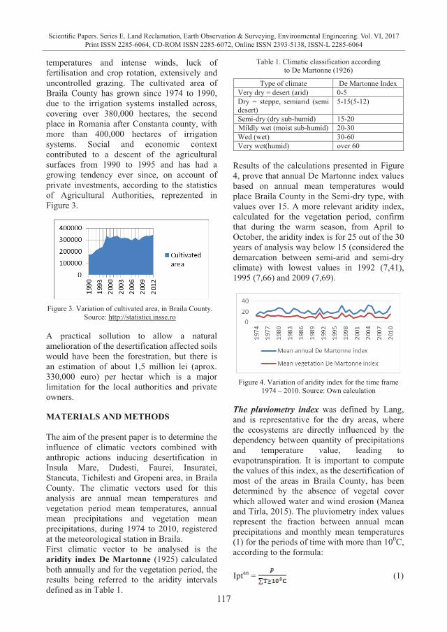
117
Scientific Papers. Series E. Land Reclamation, Earth Observation & Surveying, Environmental Engineering. Vol. VI, 2017Print ISSN 2285-6064, CD-ROM ISSN 2285-6072, Online ISSN 2393-5138, ISSN-L 2285-6064
temperatures and intense winds, luck of fertilisation and crop rotation, extensively and uncontrolled grazing. The cultivated area of Braila County has grown since 1974 to 1990, due to the irrigation systems installed across, covering over 380,000 hectares, the second place in Romania after Constanta county, with more than 400,000 hectares of irrigation systems. Social and economic context contributed to a descent of the agricultural surfaces from 1990 to 1995 and has had a growing tendency ever since, on account of private investments, according to the statistics of Agricultural Authorities, reprezented in Figure 3.
Figure 3. Variation of cultivated area, in Braila County.
Source: http://statistici.insse.ro A practical sollution to allow a natural amelioration of the desertification affected soils would have been the forestration, but there is an estimation of about 1,5 million lei (aprox. 330,000 euro) per hectar which is a major limitation for the local authorities and private owners. MATERIALS AND METHODS The aim of the present paper is to determine the influence of climatic vectors combined with anthropic actions inducing desertification in Insula Mare, Dudesti, Faurei, Insuratei, Stancuta, Tichilesti and Gropeni area, in Braila County. The climatic vectors used for this analysis are annual mean temperatures and vegetation period mean temperatures, annual mean precipitations and vegetation mean precipitations, during 1974 to 2010, registered at the meteorological station in Braila. First climatic vector to be analysed is the aridity index De Martonne (1925) calculated both annually and for the vegetation period, the results being referred to the aridity intervals defined as in Table 1.
Table 1. Climatic classification according to De Martonne (1926)
Type of climate De Martonne Index Very dry = desert (arid) 0-5 Dry = steppe, semiarid (semi desert)
5-15(5-12)
Semi-dry (dry sub-humid) 15-20 Mildly wet (moist sub-humid) 20-30 Wed (wet) 30-60 Very wet(humid) over 60
Results of the calculations presented in Figure 4, prove that annual De Martonne index values based on annual mean temperatures would place Braila County in the Semi-dry type, with values over 15. A more relevant aridity index, calculated for the vegetation period, confirm that during the warm season, from April to October, the aridity index is for 25 out of the 30 years of analysis way below 15 (considered the demarcation between semi-arid and semi-dry climate) with lowest values in 1992 (7,41), 1995 (7,66) and 2009 (7,69).
Figure 4. Variation of aridity index for the time frame
1974 – 2010. Source: Own calculation The pluviometry index was defined by Lang, and is representative for the dry areas, where the ecosystems are directly influenced by the dependency between quantity of precipitations and temperature value, leading to evapotranspiration. It is important to compute the values of this index, as the desertification of most of the areas in Braila County, has been determined by the absence of vegetal cover which allowed water and wind erosion (Manea and Tirla, 2015). The pluviometry index values represent the fraction between annual mean precipitations and monthly mean temperatures (1) for the periods of time with more than 100C, according to the formula: Iptan = (1)
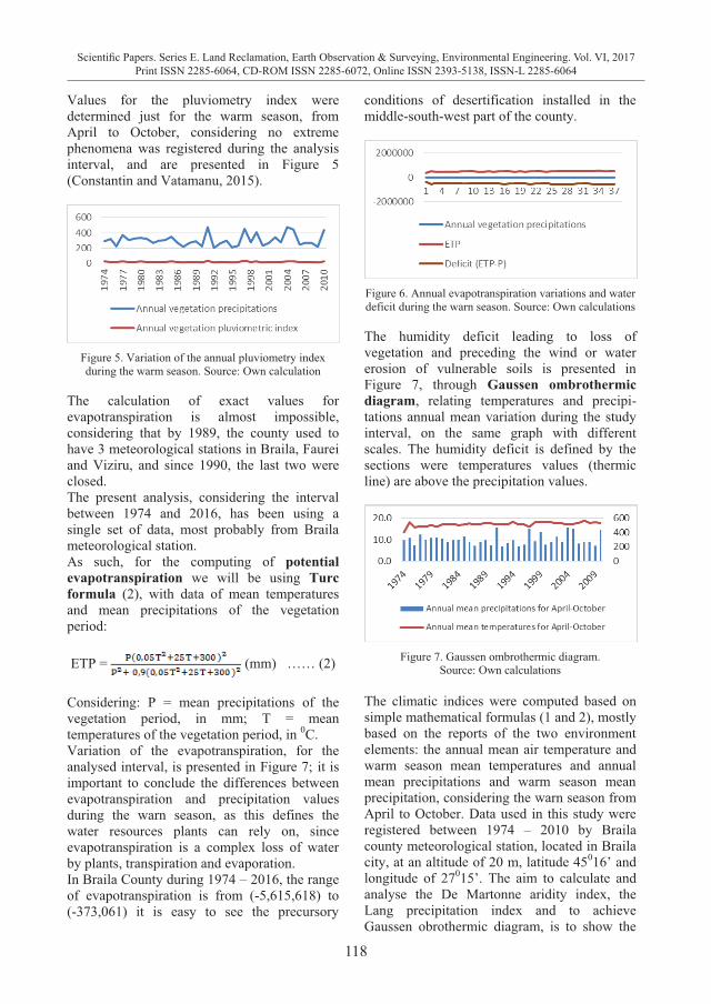
118
Scientific Papers. Series E. Land Reclamation, Earth Observation & Surveying, Environmental Engineering. Vol. VI, 2017Print ISSN 2285-6064, CD-ROM ISSN 2285-6072, Online ISSN 2393-5138, ISSN-L 2285-6064
Values for the pluviometry index were determined just for the warm season, from April to October, considering no extreme phenomena was registered during the analysis interval, and are presented in Figure 5 (Constantin and Vatamanu, 2015).
Figure 5. Variation of the annual pluviometry index during the warm season. Source: Own calculation
The calculation of exact values for evapotranspiration is almost impossible, considering that by 1989, the county used to have 3 meteorological stations in Braila, Faurei and Viziru, and since 1990, the last two were closed. The present analysis, considering the interval between 1974 and 2016, has been using a single set of data, most probably from Braila meteorological station. As such, for the computing of potential evapotranspiration we will be using Turc formula (2), with data of mean temperatures and mean precipitations of the vegetation period: ETP = (mm) …… (2)
Considering: P = mean precipitations of the vegetation period, in mm; T = mean temperatures of the vegetation period, in 0C. Variation of the evapotranspiration, for the analysed interval, is presented in Figure 7; it is important to conclude the differences between evapotranspiration and precipitation values during the warn season, as this defines the water resources plants can rely on, since evapotranspiration is a complex loss of water by plants, transpiration and evaporation. In Braila County during 1974 – 2016, the range of evapotranspiration is from (-5,615,618) to (-373,061) it is easy to see the precursory
conditions of desertification installed in the middle-south-west part of the county.
Figure 6. Annual evapotranspiration variations and water deficit during the warn season. Source: Own calculations The humidity deficit leading to loss of vegetation and preceding the wind or water erosion of vulnerable soils is presented in Figure 7, through Gaussen ombrothermic diagram, relating temperatures and precipi-tations annual mean variation during the study interval, on the same graph with different scales. The humidity deficit is defined by the sections were temperatures values (thermic line) are above the precipitation values.
Figure 7. Gaussen ombrothermic diagram.
Source: Own calculations The climatic indices were computed based on simple mathematical formulas (1 and 2), mostly based on the reports of the two environment elements: the annual mean air temperature and warm season mean temperatures and annual mean precipitations and warm season mean precipitation, considering the warn season from April to October. Data used in this study were registered between 1974 – 2010 by Braila county meteorological station, located in Braila city, at an altitude of 20 m, latitude 45016’ and longitude of 27015’. The aim to calculate and analyse the De Martonne aridity index, the Lang precipitation index and to achieve Gaussen obrothermic diagram, is to show the
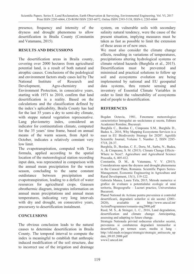
119
Scientific Papers. Series E. Land Reclamation, Earth Observation & Surveying, Environmental Engineering. Vol. VI, 2017Print ISSN 2285-6064, CD-ROM ISSN 2285-6072, Online ISSN 2393-5138, ISSN-L 2285-6064
presence, frequency and intensity of the dryness and drought phenomena to allow desertification in Braila County (Constantin and Vatamanu, 2015). RESULTS AND DISCUSSIONS The desertification areas in Braila county, covering over 2000 hectares from agricultural potential land, is a result of both natural and atrophic causes. Conclusions of the pedological and environment factors study cases led by The National Institute of Research and Development, Agro-chemistry and Environment Protection, in consecutive years, starting with 1971 to 2010, confirm that land desertification is a reality. Based on the calculations and the classification defined by the index’s aplicability, Braila County has had for the last 35 years a dry to semi-dry climate, with steppe natural vegetation represenative. Lang pluviometry index, considered an indicator for continentalism climate, computed for the 35 years’ time frame, based on annual means of the warm season, from April to October, indicates a relatively constant very low limit. The evapotranspiration, computed with Turc formula, applied according to the spatial location of the meteorological station recording input data, was represented in comparison with the annual mean precipitation for the warm season, concluding to the same constant outdistance between precipitation and evapotranspiration, leading to a deficit of water resources for agricultural crops. Gaussen obrothermic diagram, integrates information on annual mean precipitations and annual mean temperatures, indicating very long intervals with dry and drought, on consecutive years, precursory to desertification instalment. CONCLUSIONS The obvious conclusion leads to the natural causes to determine desertification in Braila County. The temporal interval to compute the index is meaningful to establish that anthropic induced modification of the soil structure, due to incorrect use of the irrigation and drainage
system, on vulnerable soils with secondary salinity natural tendency, were the cause of the present situation, implying measures must be taken as fast as possible to limit the extension of these areas or of new ones. We must also consider the climate change effects, resulting in variations of temperatures, precipitations altering hydrological systems or climate related hazards (Burghila et al., 2015). Desertification must be prevented and minimised and practical solutions to follow up soil and ecosystems evolution are being implemented by national and EU geospatial data systems, thru remote sensing and inventory of Essential Climate Variables in order to limit the vulnerability of ecosystems and of people to desertification. REFERENCES Bogdan Octavia, 1981, Fenomene meteorologice caracteristice întregului an–uscăciunea și seceta, Editura Academiei Române, București. Burghila C., Bordun C., Cimpeanu S.M., Burghila D., Badea A., 2016, Why Mapping Ecosystems Services is a must in EU Biodiversity Strategy for 2020?. Agrolife Scientific Journal, Volume 5, Number 2, ISSN 2285-5718, 28-37. Burghila, D., Bordun, C. E., Doru, M., Sarbu, N., Badea, A., & Cimpeanu, S. M. (2015). Climate Change Effects–Where to Next?. Agriculture and Agricultural Science Procedia, 6, 405-412. Constantin, D. M., & Vatamanu, V. V. (2015). Considerations upon the dryness and drought phenomena in the Caracal Plain, Romania. Scientific Papers Series-Management, Economic Engineering in Agriculture and Rural Development, 15(1), 119-122. Gabriela Manea, Laura Tirla, 2015, Metode numerice si grafice de evaluare a potentialului ecologic al unui teritoriu, Biogeografie – Lucrari practice, Universitatea Bucuresti. Planul National de Actiune pentru prevenirea si controlul desertificarii, degradarii solurilor si ale secetei (2001-2020), available at http://www.unccd.int/ ActionProgrammes/romania-eng2000.pdf Reed, M. S., & Stringer, L. C., 2016, Land degradation, desertification and climate change: Anticipating, assessing and adapting to future change. Strategia Nationala privind reducerea efectelor secetei, prevenirea si combaterea degradarii terenurilor si desertificarii, pe termen scurt, mediu si lung - http://old.madr.ro/pages/strategie/strategie_antiseceta_update_09.05.2008.pdf www2.unccd.int/
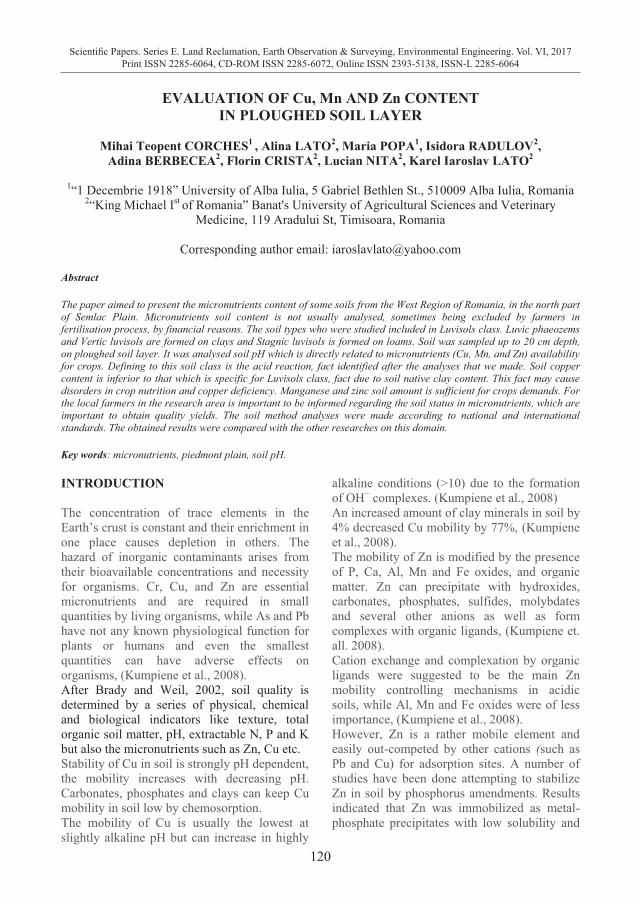
120
Scientific Papers. Series E. Land Reclamation, Earth Observation & Surveying, Environmental Engineering. Vol. VI, 2017Print ISSN 2285-6064, CD-ROM ISSN 2285-6072, Online ISSN 2393-5138, ISSN-L 2285-6064
EVALUATION OF Cu, Mn AND Zn CONTENT
IN PLOUGHED SOIL LAYER
Mihai Teopent CORCHES1 , Alina LATO2, Maria POPA1, Isidora RADULOV2, Adina BERBECEA2, Florin CRISTA2, Lucian NITA2, Karel Iaroslav LATO2
1“1 Decembrie 1918” University of Alba Iulia, 5 Gabriel Bethlen St., 510009 Alba Iulia, Romania
2“King Michael Ist of Romania” Banat's University of Agricultural Sciences and Veterinary Medicine, 119 Aradului St, Timisoara, Romania
Corresponding author email: [email protected]
Abstract The paper aimed to present the micronutrients content of some soils from the West Region of Romania, in the north part of Semlac Plain. Micronutrients soil content is not usually analysed, sometimes being excluded by farmers in fertilisation process, by financial reasons. The soil types who were studied included in Luvisols class. Luvic phaeozems and Vertic luvisols are formed on clays and Stagnic luvisols is formed on loams. Soil was sampled up to 20 cm depth, on ploughed soil layer. It was analysed soil pH which is directly related to micronutrients (Cu, Mn, and Zn) availability for crops. Defining to this soil class is the acid reaction, fact identified after the analyses that we made. Soil copper content is inferior to that which is specific for Luvisols class, fact due to soil native clay content. This fact may cause disorders in crop nutrition and copper deficiency. Manganese and zinc soil amount is sufficient for crops demands. For the local farmers in the research area is important to be informed regarding the soil status in micronutrients, which are important to obtain quality yields. The soil method analyses were made according to national and international standards. The obtained results were compared with the other researches on this domain. Key words: micronutrients, piedmont plain, soil pH. INTRODUCTION The concentration of trace elements in the Earth’s crust is constant and their enrichment in one place causes depletion in others. The hazard of inorganic contaminants arises from their bioavailable concentrations and necessity for organisms. Cr, Cu, and Zn are essential micronutrients and are required in small quantities by living organisms, while As and Pb have not any known physiological function for plants or humans and even the smallest quantities can have adverse effects on organisms, (Kumpiene et al., 2008). After Brady and Weil, 2002, soil quality is determined by a series of physical, chemical and biological indicators like texture, total organic soil matter, pH, extractable N, P and K but also the micronutrients such as Zn, Cu etc. Stability of Cu in soil is strongly pH dependent, the mobility increases with decreasing pH. Carbonates, phosphates and clays can keep Cu mobility in soil low by chemosorption. The mobility of Cu is usually the lowest at slightly alkaline pH but can increase in highly
alkaline conditions (>10) due to the formation of OH− complexes. (Kumpiene et al., 2008) An increased amount of clay minerals in soil by 4% decreased Cu mobility by 77%, (Kumpiene et al., 2008). The mobility of Zn is modified by the presence of P, Ca, Al, Mn and Fe oxides, and organic matter. Zn can precipitate with hydroxides, carbonates, phosphates, sulfides, molybdates and several other anions as well as form complexes with organic ligands, (Kumpiene et. all. 2008). Cation exchange and complexation by organic ligands were suggested to be the main Zn mobility controlling mechanisms in acidic soils, while Al, Mn and Fe oxides were of less importance, (Kumpiene et al., 2008). However, Zn is a rather mobile element and easily out-competed by other cations (such as Pb and Cu) for adsorption sites. A number of studies have been done attempting to stabilize Zn in soil by phosphorus amendments. Results indicated that Zn was immobilized as metal-phosphate precipitates with low solubility and
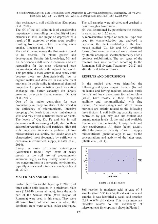
121
Scientific Papers. Series E. Land Reclamation, Earth Observation & Surveying, Environmental Engineering. Vol. VI, 2017Print ISSN 2285-6064, CD-ROM ISSN 2285-6072, Online ISSN 2393-5138, ISSN-L 2285-6064
EVALUATION OF Cu, Mn AND Zn CONTENT
IN PLOUGHED SOIL LAYER
Mihai Teopent CORCHES1 , Alina LATO2, Maria POPA1, Isidora RADULOV2, Adina BERBECEA2, Florin CRISTA2, Lucian NITA2, Karel Iaroslav LATO2
1“1 Decembrie 1918” University of Alba Iulia, 5 Gabriel Bethlen St., 510009 Alba Iulia, Romania
2“King Michael Ist of Romania” Banat's University of Agricultural Sciences and Veterinary Medicine, 119 Aradului St, Timisoara, Romania
Corresponding author email: [email protected]
Abstract The paper aimed to present the micronutrients content of some soils from the West Region of Romania, in the north part of Semlac Plain. Micronutrients soil content is not usually analysed, sometimes being excluded by farmers in fertilisation process, by financial reasons. The soil types who were studied included in Luvisols class. Luvic phaeozems and Vertic luvisols are formed on clays and Stagnic luvisols is formed on loams. Soil was sampled up to 20 cm depth, on ploughed soil layer. It was analysed soil pH which is directly related to micronutrients (Cu, Mn, and Zn) availability for crops. Defining to this soil class is the acid reaction, fact identified after the analyses that we made. Soil copper content is inferior to that which is specific for Luvisols class, fact due to soil native clay content. This fact may cause disorders in crop nutrition and copper deficiency. Manganese and zinc soil amount is sufficient for crops demands. For the local farmers in the research area is important to be informed regarding the soil status in micronutrients, which are important to obtain quality yields. The soil method analyses were made according to national and international standards. The obtained results were compared with the other researches on this domain. Key words: micronutrients, piedmont plain, soil pH. INTRODUCTION The concentration of trace elements in the Earth’s crust is constant and their enrichment in one place causes depletion in others. The hazard of inorganic contaminants arises from their bioavailable concentrations and necessity for organisms. Cr, Cu, and Zn are essential micronutrients and are required in small quantities by living organisms, while As and Pb have not any known physiological function for plants or humans and even the smallest quantities can have adverse effects on organisms, (Kumpiene et al., 2008). After Brady and Weil, 2002, soil quality is determined by a series of physical, chemical and biological indicators like texture, total organic soil matter, pH, extractable N, P and K but also the micronutrients such as Zn, Cu etc. Stability of Cu in soil is strongly pH dependent, the mobility increases with decreasing pH. Carbonates, phosphates and clays can keep Cu mobility in soil low by chemosorption. The mobility of Cu is usually the lowest at slightly alkaline pH but can increase in highly
alkaline conditions (>10) due to the formation of OH− complexes. (Kumpiene et al., 2008) An increased amount of clay minerals in soil by 4% decreased Cu mobility by 77%, (Kumpiene et al., 2008). The mobility of Zn is modified by the presence of P, Ca, Al, Mn and Fe oxides, and organic matter. Zn can precipitate with hydroxides, carbonates, phosphates, sulfides, molybdates and several other anions as well as form complexes with organic ligands, (Kumpiene et. all. 2008). Cation exchange and complexation by organic ligands were suggested to be the main Zn mobility controlling mechanisms in acidic soils, while Al, Mn and Fe oxides were of less importance, (Kumpiene et al., 2008). However, Zn is a rather mobile element and easily out-competed by other cations (such as Pb and Cu) for adsorption sites. A number of studies have been done attempting to stabilize Zn in soil by phosphorus amendments. Results indicated that Zn was immobilized as metal-phosphate precipitates with low solubility and
high resistance to soil acidification (Kumpiene et al., 2008). The pH of the soil solution is of considerable importance in controlling the solubility of trace elements in soils and might be depressed as a result of H+ excretion by plant roots possibly resulting from cation uptake exceeding anion uptake, (Linehan et al., 1985). Mn and Zn were among the first metals found to be essential for plants growth and development. Despite this knowledge, Mn and Zn deficiencies still remain common and are responsible for the most widespread crop micronutrient disorders throughout the world. This problem is more acute in acid sandy soils because these are characteristically low in organic matter and deficient in available plant nutrients. In acidic soils, fundamental chemical properties for plant nutrition (such as cation exchange and buffer capacity) are largely governed by organic matter content. (Obrador et al., 2007). One of the major constraints for crop productivity in many countries of the world is the deficiency of micronutrients. Intensive cropping often leads to nutrients’ imbalance in soils and may affect nutritional status of plants. The levels of Cu, Zn, Fe and Mn in soil decreases with increasing of pH, due to their adsorption/retention by soil particles. High pH soils may also indicate a problem of low micronutrients availability, but acidic ones are characterised most frequently by sufficient to excessive micronutrient supply, (Diatta et al., 2014). Except in cases of natural catastrophes (volcanisms, flood,), high levels of heavy metals in the soil are of predominately anthropic origin, as they usually occur at very low concentrations in a terrestrial environment, typically at trace and ultra-trace levels, (Silva et al., 2012). MATERIALS AND METHODS Surface horizons (arable layer up to 20 cm) of three acidic soils located in a piedmont plain area (135-140 meters altitude), from the north part of the Semlac Plain (West Region of Romania) were used in this study. They were all taken from cultivated soils in which the dominant crops were cereals, colza and maize.
The soil samples were air-dried and crushed to pass through a 2-mm sieve. pH was determined by potentiometric method, in water extract 1:2.5 ratio. A representative sample of each soil type was used for characterisation and analysed to determine the plant availability of the trace metals studied (Cu, Mn and Zn). Available forms of micronutrients in soil were determined by atomic absorption spectrophotometry after a previous solubilisation. The soil types of the research area were verified according to the Romanian Soil System Taxonomy (2012) and after the Soil Atlas of Europe. RESULTS AND DISCUSSIONS In the studied area were identified the following soil types: stagnic luvisols (formed on loams and having medium texture), vertic luvisols and luvic phaeozems formed on clays (which have mostly in their composition kaolinite and montmorillonite) with fine texture. Chemical changes and fate of micro-nutrients are strictly related to the following three factors: 1. soil buffering capacity mostly controlled by pH, clay and silt content and organic matter levels; 2. the total and available fractions of micronutrients; 3. crop plants and their requirements. All these factors usually affect the potential capacity of soil to supply micronutrients (quantitatively) as well as the concentrations and activity of the latter ones, (Diatta et al., 2014).
Figure 1. Soil pH values Soil reaction is moderate acid in case of 5 samples (from 5.35 to 5.64 pH values). For 6 soil samples it was identified a weak acid reaction (5.85 to 6.74 pH values). This is an important indicator related to the availability of micronutrients for crops, as it shows in Figure 1.
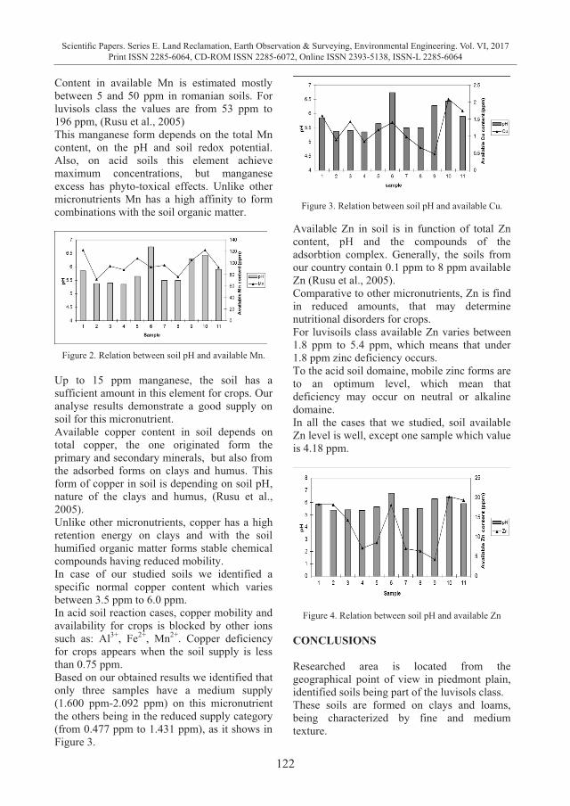
122
Scientific Papers. Series E. Land Reclamation, Earth Observation & Surveying, Environmental Engineering. Vol. VI, 2017Print ISSN 2285-6064, CD-ROM ISSN 2285-6072, Online ISSN 2393-5138, ISSN-L 2285-6064
Content in available Mn is estimated mostly between 5 and 50 ppm in romanian soils. For luvisols class the values are from 53 ppm to 196 ppm, (Rusu et al., 2005) This manganese form depends on the total Mn content, on the pH and soil redox potential. Also, on acid soils this element achieve maximum concentrations, but manganese excess has phyto-toxical effects. Unlike other micronutrients Mn has a high affinity to form combinations with the soil organic matter.
Figure 2. Relation between soil pH and available Mn.
Up to 15 ppm manganese, the soil has a sufficient amount in this element for crops. Our analyse results demonstrate a good supply on soil for this micronutrient. Available copper content in soil depends on total copper, the one originated form the primary and secondary minerals, but also from the adsorbed forms on clays and humus. This form of copper in soil is depending on soil pH, nature of the clays and humus, (Rusu et al., 2005). Unlike other micronutrients, copper has a high retention energy on clays and with the soil humified organic matter forms stable chemical compounds having reduced mobility. In case of our studied soils we identified a specific normal copper content which varies between 3.5 ppm to 6.0 ppm. In acid soil reaction cases, copper mobility and availability for crops is blocked by other ions such as: Al3+, Fe2+, Mn2+. Copper deficiency for crops appears when the soil supply is less than 0.75 ppm. Based on our obtained results we identified that only three samples have a medium supply (1.600 ppm-2.092 ppm) on this micronutrient the others being in the reduced supply category (from 0.477 ppm to 1.431 ppm), as it shows in Figure 3.
Figure 3. Relation between soil pH and available Cu.
Available Zn in soil is in function of total Zn content, pH and the compounds of the adsorbtion complex. Generally, the soils from our country contain 0.1 ppm to 8 ppm available Zn (Rusu et al., 2005). Comparative to other micronutrients, Zn is find in reduced amounts, that may determine nutritional disorders for crops. For luvisoils class available Zn varies between 1.8 ppm to 5.4 ppm, which means that under 1.8 ppm zinc deficiency occurs. To the acid soil domaine, mobile zinc forms are to an optimum level, which mean that deficiency may occur on neutral or alkaline domaine. In all the cases that we studied, soil available Zn level is well, except one sample which value is 4.18 ppm.
Figure 4. Relation between soil pH and available Zn
CONCLUSIONS Researched area is located from the geographical point of view in piedmont plain, identified soils being part of the luvisols class. These soils are formed on clays and loams, being characterized by fine and medium texture.
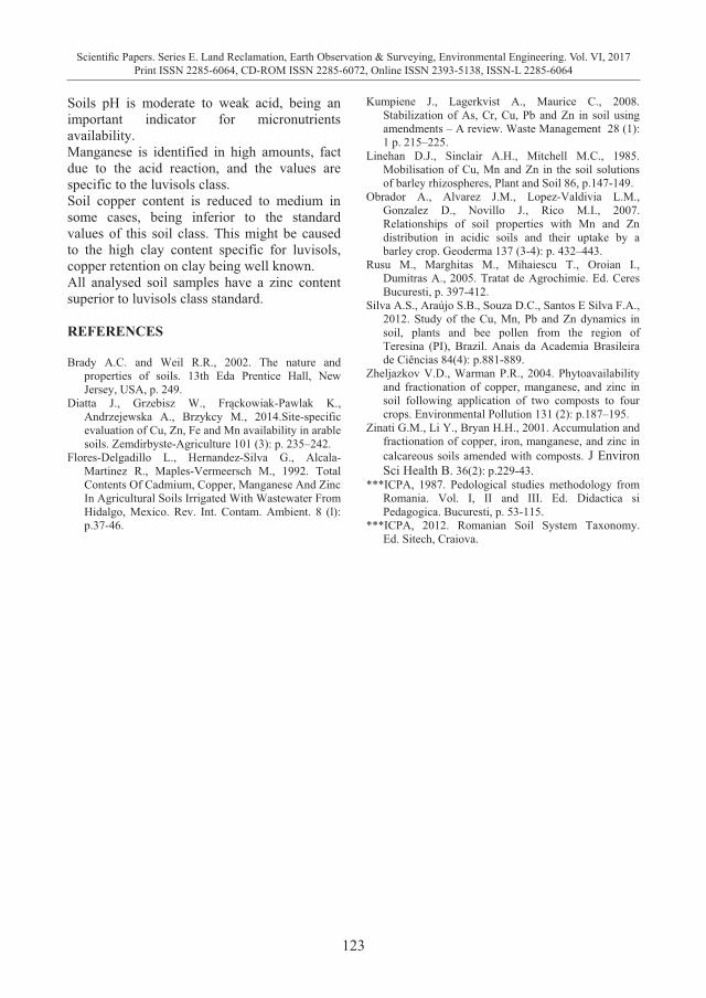
123
Scientific Papers. Series E. Land Reclamation, Earth Observation & Surveying, Environmental Engineering. Vol. VI, 2017Print ISSN 2285-6064, CD-ROM ISSN 2285-6072, Online ISSN 2393-5138, ISSN-L 2285-6064
Soils pH is moderate to weak acid, being an important indicator for micronutrients availability. Manganese is identified in high amounts, fact due to the acid reaction, and the values are specific to the luvisols class. Soil copper content is reduced to medium in some cases, being inferior to the standard values of this soil class. This might be caused to the high clay content specific for luvisols, copper retention on clay being well known. All analysed soil samples have a zinc content superior to luvisols class standard. REFERENCES Brady A.C. and Weil R.R., 2002. The nature and
properties of soils. 13th Eda Prentice Hall, New Jersey, USA, p. 249.
Diatta J., Grzebisz W., Frąckowiak-Pawlak K., Andrzejewska A., Brzykcy M., 2014.Site-specific evaluation of Cu, Zn, Fe and Mn availability in arable soils. Zemdirbyste-Agriculture 101 (3): p. 235‒242.
Flores-Delgadillo L., Hernandez-Silva G., Alcala-Martinez R., Maples-Vermeersch M., 1992. Total Contents Of Cadmium, Copper, Manganese And Zinc In Agricultural Soils Irrigated With Wastewater From Hidalgo, Mexico. Rev. Int. Contam. Ambient. 8 (l): p.37-46.
Kumpiene J., Lagerkvist A., Maurice C., 2008. Stabilization of As, Cr, Cu, Pb and Zn in soil using amendments – A review. Waste Management 28 (1): 1 p. 215–225.
Linehan D.J., Sinclair A.H., Mitchell M.C., 1985. Mobilisation of Cu, Mn and Zn in the soil solutions of barley rhizospheres, Plant and Soil 86, p.147-149.
Obrador A., Alvarez J.M., Lopez-Valdivia L.M., Gonzalez D., Novillo J., Rico M.I., 2007. Relationships of soil properties with Mn and Zn distribution in acidic soils and their uptake by a barley crop. Geoderma 137 (3-4): p. 432–443.
Rusu M., Marghitas M., Mihaiescu T., Oroian I., Dumitras A., 2005. Tratat de Agrochimie. Ed. Ceres Bucuresti, p. 397-412.
Silva A.S., Araújo S.B., Souza D.C., Santos E Silva F.A., 2012. Study of the Cu, Mn, Pb and Zn dynamics in soil, plants and bee pollen from the region of Teresina (PI), Brazil. Anais da Academia Brasileira de Ciências 84(4): p.881-889.
Zheljazkov V.D., Warman P.R., 2004. Phytoavailability and fractionation of copper, manganese, and zinc in soil following application of two composts to four crops. Environmental Pollution 131 (2): p.187–195.
Zinati G.M., Li Y., Bryan H.H., 2001. Accumulation and fractionation of copper, iron, manganese, and zinc in calcareous soils amended with composts. J Environ Sci Health B. 36(2): p.229-43.
***ICPA, 1987. Pedological studies methodology from Romania. Vol. I, II and III. Ed. Didactica si Pedagogica. Bucuresti, p. 53-115.
***ICPA, 2012. Romanian Soil System Taxonomy. Ed. Sitech, Craiova.
124
Scientific Papers. Series E. Land Reclamation, Earth Observation & Surveying, Environmental Engineering. Vol. VI, 2017Print ISSN 2285-6064, CD-ROM ISSN 2285-6072, Online ISSN 2393-5138, ISSN-L 2285-6064
SEWAGE SLUDGE COMPOSTING AND ITS AGRICULTURAL USE
Valentin FEODOROV
University of Agronomic Sciences and Veterinary Medicine of Bucharest,
59 Marasti Blvd, District 1, Bucharest, Romania
Corresponding author email: [email protected] Abstract In solid waste management, composting is defined as a controlled biological process which takes place under aerobic conditions and causes the production of simple and stable compounds in a solid substrate through the degradation of organic matter derived from animal and vegetative residues. Due to the concerns for public health and the environment, in several countries the term "composting" used in organic waste management has evolved over the years referring to the aerobic stabilization of source-separated organic matter. Sewage sludge, being a waste resulted from anthropic activities, is subject to waste regulations which prioritize their management options in order to reduce the negative environmental impacts, the ultimate option being considered the disposal into a landfill. According to the waste management hierarchy, sewage sludge has to be improved whenever possible before final disposal. Waste water treatment, mainly domestic, results in the concentration and disposal of the materials from the treated wastewater. These concentrated residual materials in admixture with water from the sewage sludge. It contains a variety of dissolved or suspension compounds: with agronomic value (compounds with nitrogen, phosphorus, potassium, calcium, magnesium, silicates, alumina, organic matter, trace elements - boron, cobalt, selenium, iodine etc), with energy value (organic matter) and potential pollutants (heavy metals, volatile organic compounds, pathogenic organisms etc). Composting sludge from sewage treatment plants represents an intensive activity and in the case of large sewage treatment plants, a large-scale activity requiring specific technologies, equipment and activities. This sludge treatment method from sewage treatment plants is an effective solution in order to significantly reduce the costs associated with disposal and also allows the production of excellent compost that can be sold for use as a natural product to improve the characteristics of soil. Key words: composting, solid waste, sludge. INTRODUCTION In solid waste management, composting is defined as a controlled biological process which takes place under aerobic conditions and causes the production of simple and stable compounds in a solid substrate through the degradation of organic matter derived from animal and vegetative residues. The solid product resulting from composting is characterized by relatively short molecular chains, a high degree of sanitization and is rich in humic compounds, making it useful for application to agricultural fields and for remaking the concentration of organic matters in soil (Metcalf & Eddy, 2003). In the composting process, microorganisms use oxygen to convert organic matter into compost, producing in the same time carbon dioxide (C02), water, nitrate (NO3), sulfate (S04
2-) and heat. This relationship can be generally represented by the following formula:
Organic matter + O2 → compost + CO2 + H2O + NO3 + SO4
2- + heat Nowadays, composting is an interesting area from many points of view, such as: - Environment-Ecology: By composting, or-ganic matter derived from sludge from sewage treatment plants transforms into useful pro-ducts for agriculture which are characterized by high content of nutrients, soil structuring properties and low phytotoxicity; - Hygiene: During the process, high tempe-ratures are reached consequently destroying pathogens and germs; - Energy: The process uses the energy released by destroying the biochemical bonds in the organic matter (Chiumenti et al., 2005). Due to the concerns for public health and the environment, in several countries the term "composting" used in organic waste mana-gement has evolved over the years referring to the aerobic stabilization of source-separated organic matter.
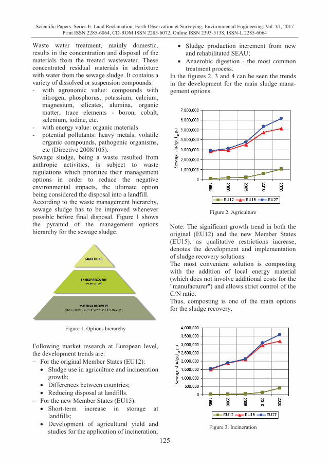
125
Scientific Papers. Series E. Land Reclamation, Earth Observation & Surveying, Environmental Engineering. Vol. VI, 2017Print ISSN 2285-6064, CD-ROM ISSN 2285-6072, Online ISSN 2393-5138, ISSN-L 2285-6064
Waste water treatment, mainly domestic, results in the concentration and disposal of the materials from the treated wastewater. These concentrated residual materials in admixture with water from the sewage sludge. It contains a variety of dissolved or suspension compounds: - with agronomic value: compounds with
nitrogen, phosphorus, potassium, calcium, magnesium, silicates, alumina, organic matter, trace elements - boron, cobalt, selenium, iodine, etc.
- with energy value: organic materials- potential pollutants: heavy metals, volatile
organic compounds, pathogenic organisms, etc (Directive 2008/105).
Sewage sludge, being a waste resulted from anthropic activities, is subject to waste regulations which prioritize their management options in order to reduce the negative environmental impacts, the ultimate option being considered the disposal into a landfill. According to the waste management hierarchy, sewage sludge has to be improved whenever possible before final disposal. Figure 1 shows the pyramid of the management options hierarchy for the sewage sludge.
Figure 1. Options hierarchy
Following market research at European level, the development trends are: � For the original Member States (EU12): � Sludge use in agriculture and incineration
growth; � Differences between countries; � Reducing disposal at landfills.
� For the new Member States (EU15): � Short-term increase in storage at
landfills; � Development of agricultural yield and
studies for the application of incineration;
� Sludge production increment from new and rehabilitated SEAU;
� Anaerobic digestion - the most common treatment process.
In the figures 2, 3 and 4 can be seen the trends in the development for the main sludge mana-gement options.
Figure 2. Agriculture
Note: The significant growth trend in both the original (EU12) and the new Member States (EU15), as qualitative restrictions increase, denotes the development and implementation of sludge recovery solutions. The most convenient solution is composting with the addition of local energy material (which does not involve additional costs for the "manufacturer") and allows strict control of the C/N ratio. Thus, composting is one of the main options for the sludge recovery.
Figure 3. Incineration
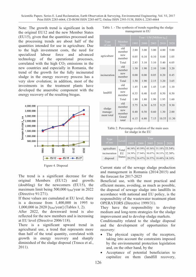
126
Scientific Papers. Series E. Land Reclamation, Earth Observation & Surveying, Environmental Engineering. Vol. VI, 2017Print ISSN 2285-6064, CD-ROM ISSN 2285-6072, Online ISSN 2393-5138, ISSN-L 2285-6064
Note: The growth trend is significant in both the original EU12 and the new Member States (EU15), given that the quantities processed and the processing trends are about half of the quantities intended for use in agriculture. Due to the high investment costs, the need for specialized labour force and advanced technology of the operational processes, correlated with the high CO2 emissions in the new countries and especially in Romania, the trend of the growth for the fully incinerated sludge in the energy recovery process has a very slow evolution; in addition, most of the investments in the treatment plants have developed the anaerobic component with the energy recovery of the resulting biogas.
Figure 4. Disposal
The trend is a significant decrease for the original Members (EU12) and growth (doubling) for the newcomers (EU15), the maximum limit being 500,000 tDM/year in 2022 (Directive 91/271). If these values are cumulated at EU level, there is a decrease from 1,400,000 in 1995 to 1,000,000 in 2020 [tDM/year] (Tables 1, 2). After 2022, the downward trend is also reflected for the new members and is increasing at EU level (Directive 2006/118). There is a significant upward trend in agricultural use, a trend that represents more than half of the total quantity, correlated with growth in energy recovery and sharply diminished of the sludge disposal (Trasca et al., 2011).
Table 1. - The synthesis of trends regarding the sludge management in EU
Year / UM [Million tSU] Type of use
Member State 1995 2000 2005 2010 2020
agriculture
old member 2.80 3.00 3.00 4.80 5.00
new member 0.05 0.10 0.10 0.60 1.05
Total 2.85 3.10 3.10 5.40 6.05
old member 1.50 1.90 2.10 3.00 3.20
incineration new member 0.00 0.00 0.05 0.20 0.45
Total 1.50 1.90 2.15 3.20 3.65
landfill
old member 1.45 1.40 1.45 1.45 1.10
new member 0.35 0.40 0.45 0.50 0.50
Total 1.80 1.80 1.90 1.95 1.60
sludge manage-
ment total
old member 5.75 6.30 6.55 9.25 9.30
new member 0.40 0.50 0.60 1.30 2.00
Grand total 6.15 6.80 7.15 10.55 11.30
Table 2. Percentage evolution of the main uses
for sludge in the EU
Type of use Level
Year
1995 2000 2005 2010 2020
agriculture Total EU
States
46.34% 45.59% 43.36% 51.18% 53.54%
incineration 24.39% 27.94% 30.07% 30.33% 32.30%
disposal 29.27% 26.47% 26.57% 18.48% 14.16%
Current state of the sewage sludge production and management in Romania (2014/2015) and the forecast for 2017-2025
� Beneficial use, with the most practical and efficient means, avoiding, as much as possible, the disposal of sewage sludge into landfills in accordance with national and EU policy, is the responsibility of the wastewater treatment plant OPERATORS (Directive 1999/31). They have the responsibility to develop medium and long-term strategies for the sludge improvement and to develop sludge markets. Conditionality related to the sludge disposal and the development of opportunities for recovery: � The physical capacity of the receptors,
taking into account the constraints imposed by the environmental protection legislation and, on the other hand, by the
� Acceptance of potential beneficiaries to capitalize on them (landfill recovery,
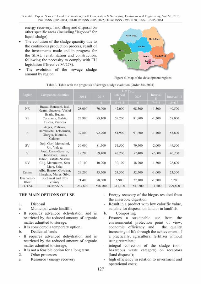
127
Scientific Papers. Series E. Land Reclamation, Earth Observation & Surveying, Environmental Engineering. Vol. VI, 2017Print ISSN 2285-6064, CD-ROM ISSN 2285-6072, Online ISSN 2393-5138, ISSN-L 2285-6064
energy recovery, landfilling and disposal on other specific areas (including "lagoons" for liquid sludge).
� The evolution of the sludge quantity due to the continuous production process, result of the investments made and in progress for the SEAU rehabilitation and construction, following the necessity to comply with EU legislation (Directive 86/278).
� The evolution of the sewage sludge amount by region.
Figure 5. Map of the development regions
Table 3. Table with the prognosis of sewage sludge evolution (Order 344/2004)
Region Component counties UM [tSU]
2014 2018 Interval I 2025 Interval
II Interval III
1 2 3 4 5 =4-3 6 7=6-4 8=6-3
NE Bacau, Botosani, Iasi, Neamt, Suceava, Vaslui 28,000 70,000 42,000 68,500 -1,500 40,500
SE Braila, Buzau,
Constanta, Galati, Tulcea, Vrancea
23,900 83,100 59,200 81,900 -1,200 58,000
S
Arges, Prahova, Dambovita, Teleorman,
Giurgiu, Ialomita, Calarasi
37,800 92,700 54,900 91,600 -1,100 53,800
SV Dolj, Gorj, Mehedinti, Olt, Valcea 30,000 81,500 51,500 79,500 -2,000 49,500
V Arad, Caras-Severin, Hunedoara, Timis 17,200 59,400 42,200 57,400 -2,000 40,200
NV Bihor, Bistrita-Nasaud, Cluj, Maramures, Satu
Mare, Salaj 10,100 40,200 30,100 38,700 -1,500 28,600
Center Alba, Brasov, Covasna, Harghita, Mures, Sibiu 29,200 53,500 24,300 52,500 -1,000 23,300
Bucharest-Ilfov
Bucharest and Ilfov county 71,400 78,300 6,900 77,100 -1,200 5,700
TOTAL ROMANIA 247,600 558,700 311,100 547,200 -11,500 299,600 THE MAIN OPTIONS OF USE 1. Disposal a. Municipal waste landfills - It requires advanced dehydration and is
restricted by the reduced amount of organic matter admitted to storage;
- It is considered a temporary option. b. Dedicated lands - It requires advanced dehydration and is
restricted by the reduced amount of organic matter admitted to storage;
- It is not a feasible option for a long term. 2. Other processes a. Resource / energy recovery
- Energy recovery of the biogas resulted from the anaerobic digestion;
- Result in a product with low calorific value, suitable for disposal on land or in landfills.
b. Composting - Ensures a sustainable use from the
environmental protection point of view, economic efficiency and the quality increasing of life through the achievement of a practically, agricultural fertilizer without using restraints;
- integral collection of the sludge (non-hazardous waste category) on receptors (land disposal);
- high efficiency in relation to investment and operational costs;
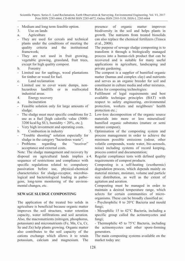
128
Scientific Papers. Series E. Land Reclamation, Earth Observation & Surveying, Environmental Engineering. Vol. VI, 2017Print ISSN 2285-6064, CD-ROM ISSN 2285-6072, Online ISSN 2393-5138, ISSN-L 2285-6064
- Medium and long term feasible option. 3. Use on lands a. Agriculture - They are used for cereals and technical
plants under the conditions of meeting the quality criteria and the institutional framework;
- They are not used in fruit growing, vegetable growing, grassland, fruit trees, except for high quality compost.
b. Forestry - Limited use for saplings, wood plantations
for timber or wood for fuel. c. Land reclamation - Limited use to cover waste dumps, non-
hazardous landfills or in reallocated industrial areas.
4. Energy recovery a. Incineration - Feasible solution only for large amounts of
sludge; - The sludge must meet specific conditions for
use as a fuel [high calorific value (3000-3200 kcal/kg SU), humidity < 20%, etc.];
- Very high investment and operating costs. b. Combustion in industry - "Trouble shooting" solution especially for
sludge in the category "hazardous waste"; - Problems regarding the “receiver”
acceptance and external costs. Note: The sludge management and recovery by disposal on agricultural lands implies a sequence of restrictions and compliance with specific regulations related to: compulsory passivation before use, physical-chemical characteristics for sludge-receptor, microbio-logical and bacteriological loading in patho-gens, long-term monitoring of the environ-mental changes, etc. SEWAGE SLUDGE COMPOSTING The application of the treated bio solids in agriculture is beneficial because organic matter improves the soil structure, water retention capacity, water infiltrations and soil aeration. Also, the macronutrients (nitrogen, phosphorus, potassium) and micronutrients (Fe, Mn, Cu, Cr, Se and Zn) help plants growing. Organic matter also contributes to the soil capacity of the cations exchange which allows it to retain potassium, calcium and magnesium. The
presence of organic matter improves biodiversity in the soil and helps plants in growth. The nutrients from treated biosolids can also replace the chemical fertilizers (Trasca et al., 2008). The purpose of sewage sludge composting is to transform it through a biologically managed process into a humus-rich product that can be recovered and is suitable for many useful applications in agriculture, landscaping and private gardening. The compost is a supplier of humified organic matter (humus and complex clay) and nutrients and serves as an organic breeder for soil and constituent in culture media and other mixtures. Rules for composting technologies:
1. Fulfilment of legal requirements and best available technique principles (BAT) with respect to safety engineering, environmental protection, workers and neighbours’ health protection etc.;
2. Low-loss decomposition of the organic source materials into more or less mineralised/ humified organic substrates (mature or semi mature compost);
3. Optimisation of the composting system and process management in order to achieve the minimum possible emissions (odour, other volatile compounds, waste water, bio-aerosols, noise) including systems of record keeping, process control and documentation;
4. Regular compliance tests with defined quality requirements of compost products. Composting is a self-heating (exothermic) degradation process, which depends mainly on material mixture, moisture, volume and particle size distribution, as well as the extent of agitation and aeration. Composting must be managed in order to maintain a desired temperature range, which selects for certain communities of micro-organisms. These can be broadly classified as: - Psychrophilic 0 to 20°C Bacteria and mould fungi; - Mesophilic 15 to 42°C Bacteria, including a specific group called the actinomycetes and fungi; - Thermophilic 45 to 75°C Bacteria, including the actinomycetes and other spore-forming generators. The main composting systems available on the market today are:
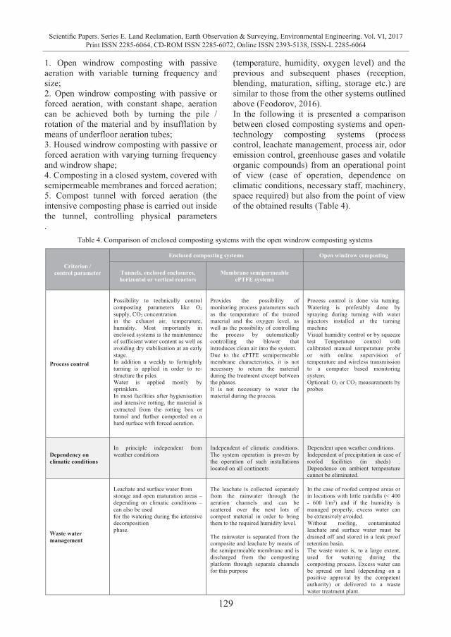
129
Scientific Papers. Series E. Land Reclamation, Earth Observation & Surveying, Environmental Engineering. Vol. VI, 2017Print ISSN 2285-6064, CD-ROM ISSN 2285-6072, Online ISSN 2393-5138, ISSN-L 2285-6064
1. Open windrow composting with passive aeration with variable turning frequency and size; 2. Open windrow composting with passive or forced aeration, with constant shape, aeration can be achieved both by turning the pile / rotation of the material and by insufflation by means of underfloor aeration tubes; 3. Housed windrow composting with passive or forced aeration with varying turning frequency and windrow shape; 4. Composting in a closed system, covered with semipermeable membranes and forced aeration; 5. Compost tunnel with forced aeration (the intensive composting phase is carried out inside the tunnel, controlling physical parameters
(temperature, humidity, oxygen level) and the previous and subsequent phases (reception, blending, maturation, sifting, storage etc.) are similar to those from the other systems outlined above (Feodorov, 2016). In the following it is presented a comparison between closed composting systems and open-technology composting systems (process control, leachate management, process air, odor emission control, greenhouse gases and volatile organic compounds) from an operational point of view (ease of operation, dependence on climatic conditions, necessary staff, machinery, space required) but also from the point of view of the obtained results (Table 4).
. Table 4. Comparison of enclosed composting systems with the open windrow composting systems
Criterion / control parameter
Enclosed composting systems Open windrow composting
Tunnels, enclosed enclosures, horizontal or vertical reactors
Membrane semipermeable ePTFE systems
Process control
Possibility to technically control composting parameters like O2 supply, CO2 concentration in the exhaust air, temperature, humidity. Most importantly in enclosed systems is the maintenance of sufficient water content as well as avoiding dry stabilisation at an early stage. In addition a weekly to fortnightly turning is applied in order to re-structure the piles. Water is applied mostly by sprinklers. In most facilities after hygienisation and intensive rotting, the material is extracted from the rotting box or tunnel and further composted on a hard surface with forced aeration.
Provides the possibility of monitoring process parameters such as the temperature of the treated material and the oxygen level, as well as the possibility of controlling the process by automatically controlling the blower that introduces clean air into the system. Due to the ePTFE semipermeable membrane characteristics, it is not necessary to return the material during the treatment except between the phases. It is not necessary to water the material during the process.
Process control is done via turning. Watering is preferably done by spraying during turning with water injectors installed at the turning machine Visual humidity control or by squeeze test Temperature control with calibrated manual temperature probe or with online supervision of temperature and wireless transmission to a computer based monitoring system. Optional: O2 or CO2 measurements by probes
Dependency on climatic conditions
In principle independent from weather conditions
Independent of climatic conditions. The system operation is proven by the operation of such installations located on all continents
Dependent upon weather conditions. Independent of precipitation in case of roofed facilities (in sheds) . Dependence on ambient temperature cannot be eliminated.
Waste water management
Leachate and surface water from storage and open maturation areas – depending on climatic conditions – can also be used for the watering during the intensive decomposition phase.
The leachate is collected separately from the rainwater through the aeration channels and can be scattered over the next lots of compost material in order to bring them to the required humidity level. The rainwater is separated from the composite and leachate by means of the semipermeable membrane and is discharged from the composting platform through separate channels for this purpose
In the case of roofed compost areas or in locations with little rainfalls (< 400 - 600 l/m²) and if the humidity is managed properly, excess water can be extensively avoided. Without roofing, contaminated leachate and surface water must be drained off and stored in a leak proof retention basin. The waste water is, to a large extent, used for watering during the composting process. Excess water can be spread on land (depending on a positive approval by the competent authority) or delivered to a waste water treatment plant.
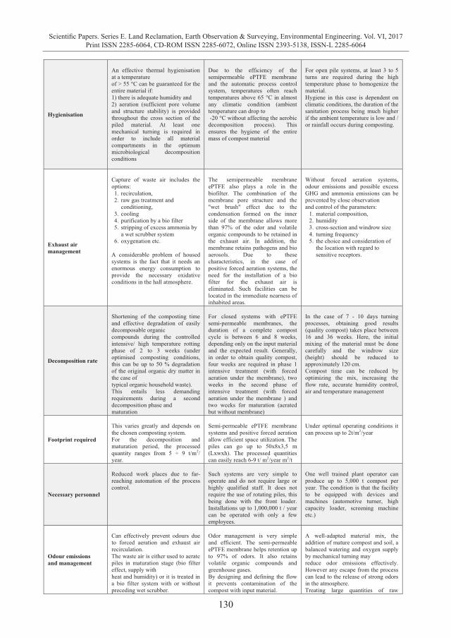
130
Scientific Papers. Series E. Land Reclamation, Earth Observation & Surveying, Environmental Engineering. Vol. VI, 2017Print ISSN 2285-6064, CD-ROM ISSN 2285-6072, Online ISSN 2393-5138, ISSN-L 2285-6064
Hygienisation
An effective thermal hygienisation at a temperature of > 55 °C can be guaranteed for the entire material if: 1) there is adequate humidity and 2) aeration (sufficient pore volume and structure stability) is provided throughout the cross section of the piled material. At least one mechanical turning is required in order to include all material compartments in the optimum microbiological decomposition conditions
Due to the efficiency of the semipermeable ePTFE membrane and the automatic process control system, temperatures often reach temperatures above 65 °C in almost any climatic condition (ambient temperature can drop to -20 °C without affecting the aerobic decomposition process). This ensures the hygiene of the entire mass of compost material
For open pile systems, at least 3 to 5 turns are required during the high temperature phase to homogenize the material. Hygiene in this case is dependent on climatic conditions, the duration of the sanitation process being much higher if the ambient temperature is low and / or rainfall occurs during composting.
Exhaust air management
Capture of waste air includes the options: 1. recirculation, 2. raw gas treatment and
conditioning, 3. cooling 4. purification by a bio filter 5. stripping of excess ammonia by
a wet scrubber system 6. oxygenation etc.
A considerable problem of housed systems is the fact that it needs an enormous energy consumption to provide the necessary oxidative conditions in the hall atmosphere.
The semipermeable membrane ePTFE also plays a role in the biofilter. The combination of the membrane pore structure and the "wet brush" effect due to the condensation formed on the inner side of the membrane allows more than 97% of the odor and volatile organic compounds to be retained in the exhaust air. In addition, the membrane retains pathogens and bio aerosols. Due to these characteristics, in the case of positive forced aeration systems, the need for the installation of a bio filter for the exhaust air is eliminated. Such facilities can be located in the immediate nearness of inhabited areas.
Without forced aeration systems, odour emissions and possible excess GHG and ammonia emissions can be prevented by close observation and control of the parameters:
1. material composition, 2. humidity 3. cross-section and windrow size 4. turning frequency 5. the choice and consideration of
the location with regard to sensitive receptors.
Decomposition rate
Shortening of the composting time and effective degradation of easily decomposable organic compounds during the controlled intensive/ high temperature rotting phase of 2 to 3 weeks (under optimised composting conditions, this can be up to 50 % degradation of the original organic dry matter in the case of typical organic household waste). This entails less demanding requirements during a second decomposition phase and maturation
For closed systems with ePTFE semi-permeable membranes, the duration of a complete compost cycle is between 6 and 8 weeks, depending only on the input material and the expected result. Generally, in order to obtain quality compost, four weeks are required in phase 1 intensive treatment (with forced aeration under the membrane), two weeks in the second phase of intensive treatment (with forced aeration under the membrane ) and two weeks for maturation (aerated but without membrane)
In the case of 7 - 10 days turning processes, obtaining good results (quality compost) takes place between 16 and 36 weeks. Here, the initial mixing of the material must be done carefully and the windrow size (height) should be reduced to approximately 120 cm. Compost time can be reduced by optimizing the mix, increasing the flow rate, accurate humidity control, air and temperature management
Footprint required
This varies greatly and depends on the chosen composting system. For the decomposition and maturation period, the processed quantity ranges from 5 ÷ 9 t/m2/ year.
Semi-permeable ePTFE membrane systems and positive forced aeration allow efficient space utilization. The piles can go up to 50x8x3,5 m (Lxwxh). The processed quantities can easily reach 6-9 t/ m2/year m2/t
Under optimal operating conditions it can process up to 2t/m2/year
Necessary personnel
Reduced work places due to far-reaching automation of the process control.
Such systems are very simple to operate and do not require large or highly qualified staff. It does not require the use of rotating piles, this being done with the front loader. Installations up to 1,000,000 t / year can be operated with only a few employees.
One well trained plant operator can produce up to 5,000 t compost per year. The condition is that the facility to be equipped with devices and machines (automotive turner, high capacity loader, screening machine etc.)
Odour emissions and management
Can effectively prevent odours due to forced aeration and exhaust air recirculation. The waste air is either used to aerate piles in maturation stage (bio filter effect, supply with heat and humidity) or it is treated in a bio filter system with or without preceding wet scrubber.
Odor management is very simple and efficient. The semi-permeable ePTFE membrane helps retention up to 97% of odors. It also retains volatile organic compounds and greenhouse gases. By designing and defining the flow it prevents contamination of the compost with input material.
A well-adapted material mix, the addition of mature compost and soil, a balanced watering and oxygen supply by mechanical turning may reduce odor emissions effectively. However any escape from the process can lead to the release of strong odors in the atmosphere. Treating large quantities of raw
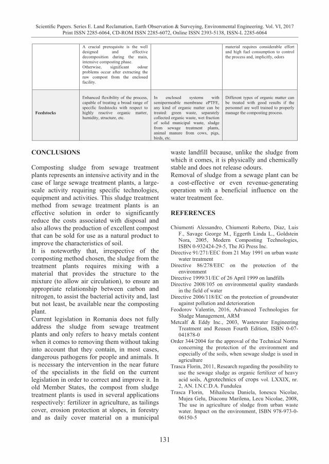
131
Scientific Papers. Series E. Land Reclamation, Earth Observation & Surveying, Environmental Engineering. Vol. VI, 2017Print ISSN 2285-6064, CD-ROM ISSN 2285-6072, Online ISSN 2393-5138, ISSN-L 2285-6064
A crucial prerequisite is the well designed and effective decomposition during the main, intensive composting phase. Otherwise, significant odour problems occur after extracting the raw compost from the enclosed facility.
material requires considerable effort and high fuel consumption to control the process and, implicitly, odors
Feedstocks
Enhanced flexibility of the process, capable of treating a broad range of specific feedstocks with respect to highly reactive organic matter, humidity, structure, etc.
In enclosed systems with semipermeable membrane ePTFE, any kind of organic matter can be treated: green waste, separately collected organic waste, wet fraction of solid municipal waste, sludge from sewage treatment plants, animal manure from cows, pigs, birds, etc.
Different types of organic matter can be treated with good results if the personnel are well trained to properly manage the composting process.
CONCLUSIONS Composting sludge from sewage treatment plants represents an intensive activity and in the case of large sewage treatment plants, a large-scale activity requiring specific technologies, equipment and activities. This sludge treatment method from sewage treatment plants is an effective solution in order to significantly reduce the costs associated with disposal and also allows the production of excellent compost that can be sold for use as a natural product to improve the characteristics of soil. It is noteworthy that, irrespective of the composting method chosen, the sludge from the treatment plants requires mixing with a material that provides the structure to the mixture (to allow air circulation), to ensure an appropriate relationship between carbon and nitrogen, to assist the bacterial activity and, last but not least, be available near the composting plant. Current legislation in Romania does not fully address the sludge from sewage treatment plants and only refers to heavy metals content when it comes to removing them without taking into account that they contain, in most cases, dangerous pathogens for people and animals. It is necessary the intervention in the near future of the specialists in the field on the current legislation in order to correct and improve it. In old Member States, the compost from sludge treatment plants is used in several applications respectively: fertilizer in agriculture, as tailings cover, erosion protection at slopes, in forestry and as daily cover material on a municipal
waste landfill because, unlike the sludge from which it comes, it is physically and chemically stable and does not release odours. Removal of sludge from a sewage plant can be a cost-effective or even revenue-generating operation with a beneficial influence on the water treatment fee. REFERENCES Chiumenti Alessandro, Chiumenti Roberto, Diaz, Luis
F., Savage George M., Eggerth Linda L., Goldstein Nora, 2005, Modern Composting Technologies, ISBN 0-932424-29-5, The JG Press Inc.
Directive 91/271/EEC from 21 May 1991 on urban waste water treatment
Directive 86/278/EEC on the protection of the environment
Directive 1999/31/EC of 26 April 1999 on landfills Directive 2008/105 on environmental quality standards
in the field of water Directive 2006/118/EC on the protection of groundwater
against pollution and deterioration Feodorov Valentin, 2016, Advanced Technologies for
Sludge Management, ARM Metcalf & Eddy Inc., 2003, Wastewater Engineering
Treatment and Reusen Fourth Edition, ISBN 0-07-041878-0
Order 344/2004 for the approval of the Technical Norms concerning the protection of the environment and especially of the soils, when sewage sludge is used in agriculture
Trasca Florin, 2011, Research regarding the possibility to use the sewage sludge as organic fertilizer of heavy acid soils, Agrotechnics of crops vol. LXXIX, nr. 2, AN. I.N.C.D.A. Fundulea
Trasca Florin, Mihailescu Daniela, Ionescu Nicolae, Mujea Gelu, Diaconu Marilena, Lecu Nicolae, 2008, The use in agriculture of sludge from urban waste water. Impact on the environment, ISBN 978-973-0-06150-5
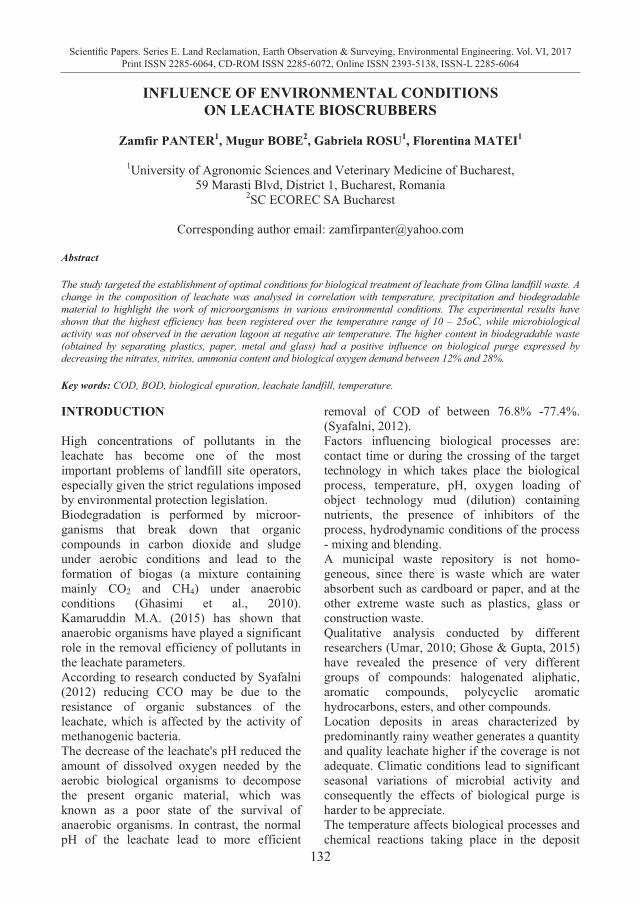
132
Scientific Papers. Series E. Land Reclamation, Earth Observation & Surveying, Environmental Engineering. Vol. VI, 2017Print ISSN 2285-6064, CD-ROM ISSN 2285-6072, Online ISSN 2393-5138, ISSN-L 2285-6064
INFLUENCE OF ENVIRONMENTAL CONDITIONS
ON LEACHATE BIOSCRUBBERS
Zamfir PANTER1, Mugur BOBE2, Gabriela ROSU1, Florentina MATEI1
1University of Agronomic Sciences and Veterinary Medicine of Bucharest,
59 Marasti Blvd, District 1, Bucharest, Romania 2SC ECOREC SA Bucharest
Corresponding author email: [email protected]
Abstract The study targeted the establishment of optimal conditions for biological treatment of leachate from Glina landfill waste. A change in the composition of leachate was analysed in correlation with temperature, precipitation and biodegradable material to highlight the work of microorganisms in various environmental conditions. The experimental results have shown that the highest efficiency has been registered over the temperature range of 10 – 25oC, while microbiological activity was not observed in the aeration lagoon at negative air temperature. The higher content in biodegradable waste (obtained by separating plastics, paper, metal and glass) had a positive influence on biological purge expressed by decreasing the nitrates, nitrites, ammonia content and biological oxygen demand between 12% and 28%. Key words: COD, BOD, biological epuration, leachate landfill, temperature. INTRODUCTION High concentrations of pollutants in the leachate has become one of the most important problems of landfill site operators, especially given the strict regulations imposed by environmental protection legislation. Biodegradation is performed by microor-ganisms that break down that organic compounds in carbon dioxide and sludge under aerobic conditions and lead to the formation of biogas (a mixture containing mainly CO2 and CH4) under anaerobic conditions (Ghasimi et al., 2010). Kamaruddin M.A. (2015) has shown that anaerobic organisms have played a significant role in the removal efficiency of pollutants in the leachate parameters. According to research conducted by Syafalni (2012) reducing CCO may be due to the resistance of organic substances of the leachate, which is affected by the activity of methanogenic bacteria. The decrease of the leachate's pH reduced the amount of dissolved oxygen needed by the aerobic biological organisms to decompose the present organic material, which was known as a poor state of the survival of anaerobic organisms. In contrast, the normal pH of the leachate lead to more efficient
removal of COD of between 76.8% -77.4%. (Syafalni, 2012). Factors influencing biological processes are: contact time or during the crossing of the target technology in which takes place the biological process, temperature, pH, oxygen loading of object technology mud (dilution) containing nutrients, the presence of inhibitors of the process, hydrodynamic conditions of the process - mixing and blending. A municipal waste repository is not homo-geneous, since there is waste which are water absorbent such as cardboard or paper, and at the other extreme waste such as plastics, glass or construction waste. Qualitative analysis conducted by different researchers (Umar, 2010; Ghose & Gupta, 2015) have revealed the presence of very different groups of compounds: halogenated aliphatic, aromatic compounds, polycyclic aromatic hydrocarbons, esters, and other compounds. Location deposits in areas characterized by predominantly rainy weather generates a quantity and quality leachate higher if the coverage is not adequate. Climatic conditions lead to significant seasonal variations of microbial activity and consequently the effects of biological purge is harder to be appreciate. The temperature affects biological processes and chemical reactions taking place in the deposit
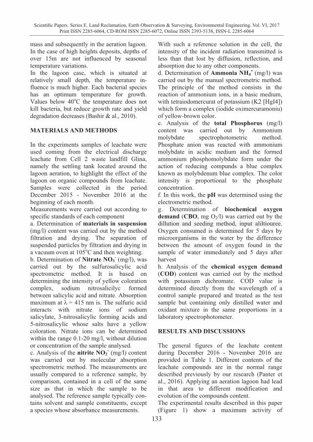
133
Scientific Papers. Series E. Land Reclamation, Earth Observation & Surveying, Environmental Engineering. Vol. VI, 2017Print ISSN 2285-6064, CD-ROM ISSN 2285-6072, Online ISSN 2393-5138, ISSN-L 2285-6064
INFLUENCE OF ENVIRONMENTAL CONDITIONS
ON LEACHATE BIOSCRUBBERS
Zamfir PANTER1, Mugur BOBE2, Gabriela ROSU1, Florentina MATEI1
1University of Agronomic Sciences and Veterinary Medicine of Bucharest,
59 Marasti Blvd, District 1, Bucharest, Romania 2SC ECOREC SA Bucharest
Corresponding author email: [email protected]
Abstract The study targeted the establishment of optimal conditions for biological treatment of leachate from Glina landfill waste. A change in the composition of leachate was analysed in correlation with temperature, precipitation and biodegradable material to highlight the work of microorganisms in various environmental conditions. The experimental results have shown that the highest efficiency has been registered over the temperature range of 10 – 25oC, while microbiological activity was not observed in the aeration lagoon at negative air temperature. The higher content in biodegradable waste (obtained by separating plastics, paper, metal and glass) had a positive influence on biological purge expressed by decreasing the nitrates, nitrites, ammonia content and biological oxygen demand between 12% and 28%. Key words: COD, BOD, biological epuration, leachate landfill, temperature. INTRODUCTION High concentrations of pollutants in the leachate has become one of the most important problems of landfill site operators, especially given the strict regulations imposed by environmental protection legislation. Biodegradation is performed by microor-ganisms that break down that organic compounds in carbon dioxide and sludge under aerobic conditions and lead to the formation of biogas (a mixture containing mainly CO2 and CH4) under anaerobic conditions (Ghasimi et al., 2010). Kamaruddin M.A. (2015) has shown that anaerobic organisms have played a significant role in the removal efficiency of pollutants in the leachate parameters. According to research conducted by Syafalni (2012) reducing CCO may be due to the resistance of organic substances of the leachate, which is affected by the activity of methanogenic bacteria. The decrease of the leachate's pH reduced the amount of dissolved oxygen needed by the aerobic biological organisms to decompose the present organic material, which was known as a poor state of the survival of anaerobic organisms. In contrast, the normal pH of the leachate lead to more efficient
removal of COD of between 76.8% -77.4%. (Syafalni, 2012). Factors influencing biological processes are: contact time or during the crossing of the target technology in which takes place the biological process, temperature, pH, oxygen loading of object technology mud (dilution) containing nutrients, the presence of inhibitors of the process, hydrodynamic conditions of the process - mixing and blending. A municipal waste repository is not homo-geneous, since there is waste which are water absorbent such as cardboard or paper, and at the other extreme waste such as plastics, glass or construction waste. Qualitative analysis conducted by different researchers (Umar, 2010; Ghose & Gupta, 2015) have revealed the presence of very different groups of compounds: halogenated aliphatic, aromatic compounds, polycyclic aromatic hydrocarbons, esters, and other compounds. Location deposits in areas characterized by predominantly rainy weather generates a quantity and quality leachate higher if the coverage is not adequate. Climatic conditions lead to significant seasonal variations of microbial activity and consequently the effects of biological purge is harder to be appreciate. The temperature affects biological processes and chemical reactions taking place in the deposit
mass and subsequently in the aeration lagoon. In the case of high heights deposits, depths of over 15m are not influenced by seasonal temperature variations. In the lagoon case, which is situated at relatively small depth, the temperature in-fluence is much higher. Each bacterial species has an optimum temperature for growth. Values below 40oC the temperature does not kill bacteria, but reduce growth rate and yield degradation decreases (Bashir & al., 2010). MATERIALS AND METHODS In the experiments samples of leachate were used coming from the electrical discharge leachate from Cell 2 waste landfill Glina, namely the settling tank located around the lagoon aeration, to highlight the effect of the lagoon on organic compounds from leachate. Samples were collected in the period December 2015 - November 2016 at the beginning of each month. Measurements were carried out according to specific standards of each component a. Determination of materials in suspension (mg/l) content was carried out by the method filtration and drying. The separation of suspended particles by filtration and drying in a vacuum oven at 105oC and then weighting. b. Determination of Nitrate NO3
- (mg/l), was carried out by the sulfurosalicylic acid spectrometric method. It is based on determining the intensity of yellow coloration complex, sodium nitrosalicilyc formed between salicylic acid and nitrate. Absorption maximum at λ = 415 nm is. The sulfuric acid interacts with nitrate ions of sodium salicylate, 3-nitrosalicylic forming acids and 5-nitrosalicylic whose salts have a yellow coloration. Nitrate ions can be determined within the range 0.1-20 mg/l, without dilution or concentration of the sample analysed. c. Analysis of the nitrite NO2
- (mg/l) content was carried out by molecular absorption spectrometric method. The measurements are usually compared to a reference sample, by comparison, contained in a cell of the same size as that in which the sample to be analysed. The reference sample typically con-tains solvent and sample constituents, except a species whose absorbance measurements.
With such a reference solution in the cell, the intensity of the incident radiation transmitted is less than that lost by diffusion, reflection, and absorption due to any other components. d. Determination of Ammonia NH4
+ (mg/l) was carried out by the manual spectrometric method. The principle of the method consists in the reaction of ammonium ions, in a basic medium, with tetraiodomercurat of potassium (K2 [HgI4]) which form a complex (iodide oximercuramoniu) of yellow-brown color. e. Analysis of the total Phosphorus (mg/l) content was carried out by Ammonium molybdate spectrophotometric method. Phosphate anion was reacted with ammonium molybdate in acidic medium and the formed ammonium phosphomolybdate form under the action of reducing compunds a blue complex known as molybdenum blue complex. The color intensity is proportional to the phosphate concentration. f. In this work, the pH was determined using the electrometric method. g. Determination of biochemical oxygen demand (CBO, mg O2/l) was carried out by the dillution and seeding method, input aliltiouree. Oxygen consumed is determined for 5 days by microorganisms in the water by the difference between the amount of oxygen found in the sample of water immediately and 5 days after harvest h. Analysis of the chemical oxygen demand (COD) content was carried out by the method with potassium dichromate. COD value is determined directly from the wavelength of a control sample prepared and treated as the test sample but containing only distilled water and oxidant mixture in the same proportions in a laboratory spectrophotometer. RESULTS AND DISCUSSIONS The general figures of the leachate content during December 2016 - November 2016 are provided in Table 1. Different contents of the leachate compounds are in the normal range described previously by our research (Panter et al., 2016). Applying an aeration lagoon had lead in that area to different modification and evolution of the compounds content. The experimental results described in this paper (Figure 1) show a maximum activity of
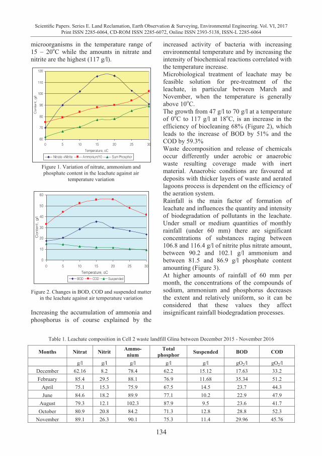
134
Scientific Papers. Series E. Land Reclamation, Earth Observation & Surveying, Environmental Engineering. Vol. VI, 2017Print ISSN 2285-6064, CD-ROM ISSN 2285-6072, Online ISSN 2393-5138, ISSN-L 2285-6064
microorganisms in the temperature range of 15 – 20oC while the amounts in nitrate and nitrite are the highest (117 g/l).
60
70
80
90
100
110
120
0 5 10 15 20 25 30Temperature, oC
Con
tent
, g/l
Nitrate +Nitrite Ammonium/10 Sum Phosphor
Figure 1. Variation of nitrate, ammonium and phosphate content in the leachate against air
temperature variation
0
10
20
30
40
50
60
0 5 10 15 20 25 30Temperature, oC
Con
tent
, g/l
BOD COD Suspended
Figure 2. Changes in BOD, COD and suspended matter in the leachate against air temperature variation
Increasing the accumulation of ammonia and phosphorus is of course explained by the
increased activity of bacteria with increasing environmental temperature and by increasing the intensity of biochemical reactions correlated with the temperature increase. Microbiological treatment of leachate may be feasible solution for pre-treatment of the leachate, in particular between March and November, when the temperature is generally above 10oC. The growth from 47 g/l to 70 g/l at a temperature of 0oC to 117 g/l at 18oC, is an increase in the efficiency of biocleaning 68% (Figure 2), which leads to the increase of BOD by 51% and the COD by 59.3% Waste decomposition and release of chemicals occur differently under aerobic or anaerobic waste resulting coverage made with inert material. Anaerobic conditions are favoured at deposits with thicker layers of waste and aerated lagoons process is dependent on the efficiency of the aeration system. Rainfall is the main factor of formation of leachate and influences the quantity and intensity of biodegradation of pollutants in the leachate. Under small or medium quantities of monthly rainfall (under 60 mm) there are significant concentrations of substances raging between 106.8 and 116.4 g/l of nitrite plus nitrate amount, between 90.2 and 102.1 g/l ammonium and between 81.5 and 86.9 g/l phosphate content amounting (Figure 3). At higher amounts of rainfall of 60 mm per month, the concentrations of the compounds of sodium, ammonium and phosphorus decreases the extent and relatively uniform, so it can be considered that these values they affect insignificant rainfall biodegradation processes.
Table 1. Leachate composition in Cell 2 waste landfill Glina between December 2015 - November 2016
Months Nitrat Nitrit Ammo- nium
Total phosphor Suspended BOD COD
g/l g/l g/l g/l g/l gO2/l gO2/l December 62.16 8.2 78.4 62.2 15.12 17.63 33.2 February 85.4 29.5 88.1 76.9 11.68 35.34 51.2
April 75.1 15.3 75.9 67.5 14.5 23.7 44.3 June 84.6 18.2 89.9 77.1 10.2 22.9 47.9
August 79.3 12.1 102.3 87.9 9.5 23.6 41.7 October 80.9 20.8 84.2 71.3 12.8 28.8 52.3
November 89.1 26.3 90.1 75.3 11.4 29.96 45.76
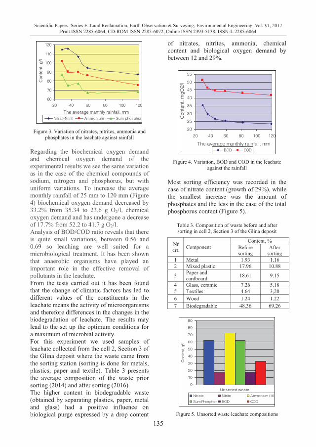
135
Scientific Papers. Series E. Land Reclamation, Earth Observation & Surveying, Environmental Engineering. Vol. VI, 2017Print ISSN 2285-6064, CD-ROM ISSN 2285-6072, Online ISSN 2393-5138, ISSN-L 2285-6064
microorganisms in the temperature range of 15 – 20oC while the amounts in nitrate and nitrite are the highest (117 g/l).
60
70
80
90
100
110
120
0 5 10 15 20 25 30Temperature, oC
Con
tent
, g/l
Nitrate +Nitrite Ammonium/10 Sum Phosphor
Figure 1. Variation of nitrate, ammonium and phosphate content in the leachate against air
temperature variation
0
10
20
30
40
50
60
0 5 10 15 20 25 30Temperature, oC
Con
tent
, g/l
BOD COD Suspended
Figure 2. Changes in BOD, COD and suspended matter in the leachate against air temperature variation
Increasing the accumulation of ammonia and phosphorus is of course explained by the
increased activity of bacteria with increasing environmental temperature and by increasing the intensity of biochemical reactions correlated with the temperature increase. Microbiological treatment of leachate may be feasible solution for pre-treatment of the leachate, in particular between March and November, when the temperature is generally above 10oC. The growth from 47 g/l to 70 g/l at a temperature of 0oC to 117 g/l at 18oC, is an increase in the efficiency of biocleaning 68% (Figure 2), which leads to the increase of BOD by 51% and the COD by 59.3% Waste decomposition and release of chemicals occur differently under aerobic or anaerobic waste resulting coverage made with inert material. Anaerobic conditions are favoured at deposits with thicker layers of waste and aerated lagoons process is dependent on the efficiency of the aeration system. Rainfall is the main factor of formation of leachate and influences the quantity and intensity of biodegradation of pollutants in the leachate. Under small or medium quantities of monthly rainfall (under 60 mm) there are significant concentrations of substances raging between 106.8 and 116.4 g/l of nitrite plus nitrate amount, between 90.2 and 102.1 g/l ammonium and between 81.5 and 86.9 g/l phosphate content amounting (Figure 3). At higher amounts of rainfall of 60 mm per month, the concentrations of the compounds of sodium, ammonium and phosphorus decreases the extent and relatively uniform, so it can be considered that these values they affect insignificant rainfall biodegradation processes.
Table 1. Leachate composition in Cell 2 waste landfill Glina between December 2015 - November 2016
Months Nitrat Nitrit Ammo- nium
Total phosphor Suspended BOD COD
g/l g/l g/l g/l g/l gO2/l gO2/l December 62.16 8.2 78.4 62.2 15.12 17.63 33.2 February 85.4 29.5 88.1 76.9 11.68 35.34 51.2
April 75.1 15.3 75.9 67.5 14.5 23.7 44.3 June 84.6 18.2 89.9 77.1 10.2 22.9 47.9
August 79.3 12.1 102.3 87.9 9.5 23.6 41.7 October 80.9 20.8 84.2 71.3 12.8 28.8 52.3
November 89.1 26.3 90.1 75.3 11.4 29.96 45.76
60
70
80
90
100
110
120
20 40 60 80 100 120The average manthly rainfall, mm
Con
tent
, g/l
Nitrat+Nitrit Ammonium Sum phosphor
Figure 3. Variation of nitrates, nitrites, ammonia and phosphates in the leachate against rainfall
Regarding the biochemical oxygen demand and chemical oxygen demand of the experimental results we see the same variation as in the case of the chemical compounds of sodium, nitrogen and phosphorus, but with uniform variations. To increase the average monthly rainfall of 25 mm to 120 mm (Figure 4) biochemical oxygen demand decreased by 33.2% from 35.34 to 23.6 g O2/l, chemical oxygen demand and has undergone a decrease of 17.7% from 52.2 to 41.7 g O2/l. Analysis of BOD/COD ratio reveals that there is quite small variations, between 0.56 and 0.69 so leaching are well suited for a microbiological treatment. It has been shown that anaerobic organisms have played an important role in the effective removal of pollutants in the leachate. From the tests carried out it has been found that the change of climatic factors has led to different values of the constituents in the leachate means the activity of microorganisms and therefore differences in the changes in the biodegradation of leachate. The results may lead to the set up the optimum conditions for a maximum of microbial activity. For this experiment we used samples of leachate collected from the cell 2, Section 3 of the Glina deposit where the waste came from the sorting station (sorting is done for metals, plastics, paper and textile). Table 3 presents the average composition of the waste prior sorting (2014) and after sorting (2016). The higher content in biodegradable waste (obtained by separating plastics, paper, metal and glass) had a positive influence on biological purge expressed by a drop content
of nitrates, nitrites, ammonia, chemical content and biological oxygen demand by between 12 and 29%.
20
25
30
35
40
45
50
55
20 40 60 80 100 120
The average manthly rainfall, mm
Cont
ent,
mgO
2/l
BOD COD Figure 4. Variation, BOD and COD in the leachate
against the rainfall Most sorting efficiency was recorded in the case of nitrate content (growth of 29%), while the smallest increase was the amount of phosphates and the less in the case of the total phosphorus content (Figure 5).
Table 3. Composition of waste before and after sorting in cell 2, Section 3 of the Glina deposit
Nr crt. Component
Content, % Before sorting
After sorting
1 Metal 1.93 1.16 2 Mixed plastic 17.96 10.88
3 Paper and cardboard 18.61 9.15
4 Glass, ceramic 7.26 5.18 5 Textiles 4.64 3,20 6 Wood 1.24 1.22 7 Biodegradable 48.36 69.26
0
10
20
30
40
50
60
70
80
90
Unsorted waste
Cont
ent, g
/l
Nitrate Nitrite Ammonium /10Sum Phosphor BOD COD
Figure 5. Unsorted waste leachate compositions
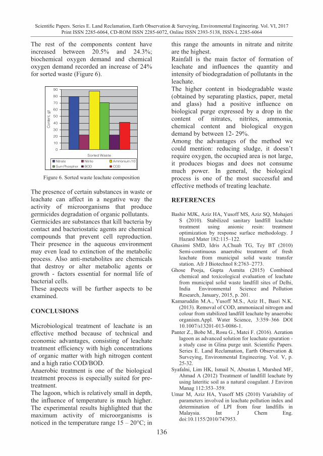
136
Scientific Papers. Series E. Land Reclamation, Earth Observation & Surveying, Environmental Engineering. Vol. VI, 2017Print ISSN 2285-6064, CD-ROM ISSN 2285-6072, Online ISSN 2393-5138, ISSN-L 2285-6064
The rest of the components content have increased between 20.5% and 24.3%; biochemical oxygen demand and chemical oxygen demand recorded an increase of 24% for sorted waste (Figure 6).
0
10
20
30
40
50
60
70
80
90
Sorted Waste
Cont
ent, g
/l
Nitrate Nitrite Ammonium /10Sum Phosphor BOD COD
Figure 6. Sorted waste leachate composition The presence of certain substances in waste or leachate can affect in a negative way the activity of microorganisms that produce germicides degradation of organic pollutants. Germicides are substances that kill bacteria by contact and bacteriostatic agents are chemical compounds that prevent cell reproduction. Their presence in the aqueous environment may even lead to extinction of the metabolic process. Also anti-metabolites are chemicals that destroy or alter metabolic agents or growth - factors essential for normal life of bacterial cells. These aspects will be further aspects to be examined. CONCLUSIONS Microbiological treatment of leachate is an effective method because of technical and economic advantages, consisting of leachate treatment efficiency with high concentrations of organic matter with high nitrogen content and a high ratio COD/BOD. Anaerobic treatment is one of the biological treatment process is especially suited for pre-treatment. The lagoon, which is relatively small in depth, the influence of temperature is much higher. The experimental results highlighted that the maximum activity of microorganisms is noticed in the temperature range 15 – 20°C; in
this range the amounts in nitrate and nitrite are the highest. Rainfall is the main factor of formation of leachate and influences the quantity and intensity of biodegradation of pollutants in the leachate. The higher content in biodegradable waste (obtained by separating plastics, paper, metal and glass) had a positive influence on biological purge expressed by a drop in the content of nitrates, nitrites, ammonia, chemical content and biological oxygen demand by between 12- 29%. Among the advantages of the method we could mention: reducing sludge, it doesn’t require oxygen, the occupied area is not large, it produces biogas and does not consume much power. In general, the biological process is one of the most successful and effective methods of treating leachate. REFERENCES Bashir MJK, Aziz HA, Yusoff MS, Aziz SQ, Mohajeri
S (2010). Stabilized sanitary landfill leachate treatment using anionic resin: treatment optimization by response surface methodology. J Hazard Mater 182:115–122.
Ghasimi SMD, Idris A,Chuah TG, Tey BT (2010) Semi-continuous anaerobic treatment of fresh leachate from municipal solid waste transfer station. Afr J Biotechnol 8:2763–2773.
Ghose Pooja, Gupta Asmita (2015) Combined chemical and toxicological evaluation of leachate from municipal solid waste landfill sites of Delhi, India Environmental Science and Pollution Research, January, 2015, p. 201.
Kamaruddin M.A., Yusoff M.S., Aziz H., Basri N.K. (2013). Removal of COD, ammoniacal nitrogen and colour from stabilized landfill leachate by anaerobic organism.Appl. Water Science, 3:359–366 DOI 10.1007/s13201-013-0086-1.
Panter Z., Bobe M., Rosu G., Matei F. (2016). Aeration lagoon as advanced solution for leachate epuration - a study case in Glina purge unit. Scientific Papers. Series E. Land Reclamation, Earth Observation & Surveying, Environmental Engineering. Vol. V, p. 25-32.
Syafalni, Lim HK, Ismail N, Abustan I, Murshed MF, Ahmad A (2012) Treatment of landfill leachate by using lateritic soil as a natural coagulant. J Environ Manag 112:353–359.
Umar M, Aziz HA, Yusoff MS (2010) Variability of parameters involved in leachate pollution index and determination of LPI from four landfills in Malaysia. Int J Chem Eng. doi:10.1155/2010/747953.
137
Scientific Papers. Series E. Land Reclamation, Earth Observation & Surveying, Environmental Engineering. Vol. VI, 2017Print ISSN 2285-6064, CD-ROM ISSN 2285-6072, Online ISSN 2393-5138, ISSN-L 2285-6064
The rest of the components content have increased between 20.5% and 24.3%; biochemical oxygen demand and chemical oxygen demand recorded an increase of 24% for sorted waste (Figure 6).
0
10
20
30
40
50
60
70
80
90
Sorted Waste
Cont
ent, g
/l
Nitrate Nitrite Ammonium /10Sum Phosphor BOD COD
Figure 6. Sorted waste leachate composition The presence of certain substances in waste or leachate can affect in a negative way the activity of microorganisms that produce germicides degradation of organic pollutants. Germicides are substances that kill bacteria by contact and bacteriostatic agents are chemical compounds that prevent cell reproduction. Their presence in the aqueous environment may even lead to extinction of the metabolic process. Also anti-metabolites are chemicals that destroy or alter metabolic agents or growth - factors essential for normal life of bacterial cells. These aspects will be further aspects to be examined. CONCLUSIONS Microbiological treatment of leachate is an effective method because of technical and economic advantages, consisting of leachate treatment efficiency with high concentrations of organic matter with high nitrogen content and a high ratio COD/BOD. Anaerobic treatment is one of the biological treatment process is especially suited for pre-treatment. The lagoon, which is relatively small in depth, the influence of temperature is much higher. The experimental results highlighted that the maximum activity of microorganisms is noticed in the temperature range 15 – 20°C; in
this range the amounts in nitrate and nitrite are the highest. Rainfall is the main factor of formation of leachate and influences the quantity and intensity of biodegradation of pollutants in the leachate. The higher content in biodegradable waste (obtained by separating plastics, paper, metal and glass) had a positive influence on biological purge expressed by a drop in the content of nitrates, nitrites, ammonia, chemical content and biological oxygen demand by between 12- 29%. Among the advantages of the method we could mention: reducing sludge, it doesn’t require oxygen, the occupied area is not large, it produces biogas and does not consume much power. In general, the biological process is one of the most successful and effective methods of treating leachate. REFERENCES Bashir MJK, Aziz HA, Yusoff MS, Aziz SQ, Mohajeri
S (2010). Stabilized sanitary landfill leachate treatment using anionic resin: treatment optimization by response surface methodology. J Hazard Mater 182:115–122.
Ghasimi SMD, Idris A,Chuah TG, Tey BT (2010) Semi-continuous anaerobic treatment of fresh leachate from municipal solid waste transfer station. Afr J Biotechnol 8:2763–2773.
Ghose Pooja, Gupta Asmita (2015) Combined chemical and toxicological evaluation of leachate from municipal solid waste landfill sites of Delhi, India Environmental Science and Pollution Research, January, 2015, p. 201.
Kamaruddin M.A., Yusoff M.S., Aziz H., Basri N.K. (2013). Removal of COD, ammoniacal nitrogen and colour from stabilized landfill leachate by anaerobic organism.Appl. Water Science, 3:359–366 DOI 10.1007/s13201-013-0086-1.
Panter Z., Bobe M., Rosu G., Matei F. (2016). Aeration lagoon as advanced solution for leachate epuration - a study case in Glina purge unit. Scientific Papers. Series E. Land Reclamation, Earth Observation & Surveying, Environmental Engineering. Vol. V, p. 25-32.
Syafalni, Lim HK, Ismail N, Abustan I, Murshed MF, Ahmad A (2012) Treatment of landfill leachate by using lateritic soil as a natural coagulant. J Environ Manag 112:353–359.
Umar M, Aziz HA, Yusoff MS (2010) Variability of parameters involved in leachate pollution index and determination of LPI from four landfills in Malaysia. Int J Chem Eng. doi:10.1155/2010/747953.
STUDY ON PEROXIDE VALUES FOR DIFFERENT OILS
AND FACTORS AFFECTING THE QUALITY OF SUNFLOWER OIL
Maria POPA1, Ioana GLEVITZKY2, Gabriela-Alina DUMITREL3, Mirel GLEVITZKY1, Dorin POPA1
1 “1 Decembrie 1918” University of Alba Iulia, 11-13 Nicolae Iorga St., 510009 Alba Iulia,
Romania 2Alba Sanitary-Veterinary and Food Safety Directorate, 7A Lalelelor St., 510217 Alba Iulia,
Romania 3Politehnica University of Timisoara, 6 Vasile Parvan Blvd., 300223 Timisoara, Romania
Corresponding author email: [email protected]
Abstract The aim of this paper is to evaluate the peroxide value (PV) of different alimentary oils, as well as to determinate the number of yeasts and molds that develops in this oils. Fungi value is an indicator that ensure the sanitation of samples. Also for refined sun flower oil, the oxidation rate of the samples exposed to daylight or kept in darkness was followed for 60 days. PV exceeds the maximum recommended value of 10 meq/kg after 45 days for sunflower oil exposed to daylight. The samples stored in the dark reached the value of 8.68 mEq/kg at the end of the investigation period. Oxidative rate of used refined sunflower oil subjected to frying temperatures (1700C) was motorized during heat treatment, finding a rapid increase in PV at 18.32 meq/kg after 60 minutes. Key words: alimentary oils, oxidative deterioration, peroxide value INTRODUCTION Oxidation of fats and oils is an important indicator for performance and shelf life of oils (Marina et al., 2013). The oxidation process is complex, dependent on the light intensity and temperature. In the first stage is formed hydro peroxides, peroxides, and then polymers of peroxides (Lupea, 2004). The PV is applicable for monitoring the formation of peroxides in the early stages of oxidation. However, the accuracy of the method is questionable since the results are depending on the process used, on the temperature at which the determinations are made. During oxidation the PV may reach a maximum and then decreases (Abramovic et al., 2005). Recommended limits that have been set for the quality oils are: PV less than 3 when the oil leaves the factory, less than 5 after the bottle it’s open and less than 10 in use. Generally, the values are substantially lower than that. PV is used only in the case of oil that is not rancid. The reason why it might be possible like the PV to have low level and still to have a rancid
oil is because, in reality, in oil are more degraded compounds than results during the decomposition, which is not seen in the respective index values. Various volatile oxidation products are compounds that contribute to the taste and odor of edible oils. The quality of the oils, inclusive physic-chemical parameters as the PV, were regulated by Romanian Decree no. 454/917/22 form 2001 (D. 454; 917; 22/2001), but the Decree no. 10/2013 repeal the most of the parameters that have a role in characterization of the oils. Also, section 2 of Codex Standards for Fats and Oils from Vegetable Sources - Codex Standard for Named Vegetable Oils, show the quality characteristics for PV in refined oils that are up to 10 milliequivalents of active oxygen/kg oil, and for cold pressed and virgin oils being up to 15 milliequivalents of active oxygen/kg oil (CODEX-STAN 210 - 1999). Variations of PV can arise from different factors such as the degree of unsaturation of the fatty acids present in the particular oil, storage, exposure to light, and the content of metals or other compounds that may catalyze the oxidation processes (Choe and Min, 2006).
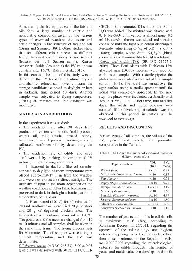
138
Scientific Papers. Series E. Land Reclamation, Earth Observation & Surveying, Environmental Engineering. Vol. VI, 2017Print ISSN 2285-6064, CD-ROM ISSN 2285-6072, Online ISSN 2393-5138, ISSN-L 2285-6064
Also, during the frying process of the fats and oils form a large number of volatile and nonvolatile compounds given by the various types of chemical reactions that occur and cause changes in the structure of fats and oils (Drum and Spanier, 1991). Other studies show that for different oils subjected to different frying temperatures in many cases (except Seasons corn oil, Season canola, Kausar banaspati, Dalda Groundnut) the PV value was constant after 130°C (Kaleem et al., 2015). In this context, the aim of this study was to determine the PV for different alimentary oil and also for refined sun flower oil using the storage conditions: exposed to daylight or kept in darkness, time period 60 days. Another sample was subjected to frying temperatures (1700C) 60 minutes and lipid oxidation was monitored. MATERIALS AND METHODS In the experiment it was studied: - The oxidation rate after 30 days from production for ten edible oils (cold pressed: walnut oil, milk thistle, linseed, poppy, hempseed, mustard, pumpkin, sesame, almond, rafinated: sunflower oil) by determining the PV, - The oxidation rate of edible and used sunflower oil, by tracking the variation of PV in time, in the following conditions:
1. Exposed to daylight (the oil samples exposed to daylight, at room temperature were placed approximately 1 m from the window and were not exposed to direct sunlight. The intensity of light in the room depended on the weather conditions in Alba Iulia, Romania) and preserved to dark in dark glass bottles, at room temperature, for 60 days;
2. Heat treated (170�C) for 60 minutes. In 200 ml sunflower oil were fried 20 g potatoes and 20 g of degassed chicken meat. The temperature is maintained constant at 170�C. The potatoes and the meat are changed from 10 to 10 minutes and oil samples shall be taken in the same time frame. The frying process lasts for 60 minutes. The oil samples were cooling at ambient temperature and the PV was determinate. PV determination (AOAC 965.33). 5.00 ± 0.05 g of oil was dissolved with 30 ml CH3COOH-
CHCl3. 0.5 ml saturated KI solution and 30 ml H2O was added. The mixture was titrated with 0.1N Na2S2O3 until yellow is almost gone. 0.5 ml 1% starch solution was added and titration continued until the light blue colour discharged. Peroxide value (meq O2/kg of oil) = S x N x 1000/g sample, where S=ml Na2S2O3 (blank corrected) and N=normality Na2S2O3 solution. Yeasts and molds (YM) (SR ISO 21527-2: 2009). Three Petri plates with Dichloran 18% glycerol agar (DG18) medium were used for each tested samples. With a sterile pipette, the plates were inoculated with 1 ml of test sample (dilution 10-1). The liquid was spread over the agar surface using a sterile spreader until the liquid was completely absorbed. In the next step, the plates were incubated aerobically with lids up at 25°C + 1°C. After three, four and five days, the yeasts and molds colonies were counted. If the developing of colonies was not observed in this period, incubation will be extended to seven days. RESULTS AND DISCUSSIONS For ten types of oil samples, the values of the PV, yeasts and molds, are presented comparative in the Table 1.
Table 1. The PV and the number of yeasts and molds for
different types of oils
The number of yeasts and molds in edibles oils is maximum 1x10² cfu/g, according to Romanian Decree nr. 27/2011, regarding the approval of the microbiology and hygiene criteria’s applying to edibles products, others then those mentioned in the Regulation (CE) no. 2.073/2005 regarding the microbiological criteria’s for edible products. The number of yeasts and molds value that develops in this oils
Type of seeds oil YM, cfu/g
PV, meq/g
Walnut (Nux) 5 x 10² 0.27 Milk thistle (Silybum marianum) < 10 0.17 Flax (Linum) < 10 0.24 Poppy (Papaver somniferum) 1 x 10 0.97 Hemp (Cannabis sativa) 1.4 x 10 3.19 Mustard (Sinapis alba) < 10 1.60 Pumpkin (Cucurbita maxima) 6 x 10 4.99 Sesame (Sesamum indicum) 1 x 10 1,80 Almonds (Prunus dulcis) 2.1 x 10 1.00 Sunflower (Helianthus annuus) < 10 1.18
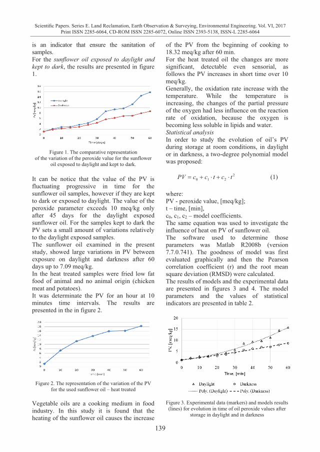
139
Scientific Papers. Series E. Land Reclamation, Earth Observation & Surveying, Environmental Engineering. Vol. VI, 2017Print ISSN 2285-6064, CD-ROM ISSN 2285-6072, Online ISSN 2393-5138, ISSN-L 2285-6064
is an indicator that ensure the sanitation of samples. For the sunflower oil exposed to daylight and kept to dark, the results are presented in figure 1.
Figure 1. The comparative representation
of the variation of the peroxide value for the sunflower oil exposed to daylight and kept to dark.
It can be notice that the value of the PV is fluctuating progressive in time for the sunflower oil samples, however if they are kept to dark or exposed to daylight. The value of the peroxide parameter exceeds 10 meq/kg only after 45 days for the daylight exposed sunflower oil. For the samples kept to dark the PV sets a small amount of variations relatively to the daylight exposed samples. The sunflower oil examined in the present study, showed large variations in PV between exposure on daylight and darkness after 60 days up to 7.09 meq/kg. In the heat treated samples were fried low fat food of animal and no animal origin (chicken meat and potatoes). It was determinate the PV for an hour at 10 minutes time intervals. The results are presented in the in figure 2.
Figure 2. The representation of the variation of the PV
for the used sunflower oil – heat treated Vegetable oils are a cooking medium in food industry. In this study it is found that the heating of the sunflower oil causes the increase
of the PV from the beginning of cooking to 18.32 meq/kg after 60 min. For the heat treated oil the changes are more significant, detectable even sensorial, as follows the PV increases in short time over 10 meq/kg. Generally, the oxidation rate increase with the temperature. While the temperature is increasing, the changes of the partial pressure of the oxygen had less influence on the reaction rate of oxidation, because the oxygen is becoming less soluble in lipids and water. Statistical analysis In order to study the evolution of oil’s PV during storage at room conditions, in daylight or in darkness, a two-degree polynomial model was proposed:
2210 tctccPV ����� (1)
where: PV - peroxide value, [meq/kg]; t – time, [min], c0, c1, c2 – model coefficients. The same equation was used to investigate the influence of heat on PV of sunflower oil. The software used to determine those parameters was Matlab R2008b (version 7.7.0.741). The goodness of model was first evaluated graphically and then the Pearson correlation coefficient (r) and the root mean square deviation (RMSD) were calculated. The results of models and the experimental data are presented in figures 3 and 4. The model parameters and the values of statistical indicators are presented in table 2.
Figure 3. Experimental data (markers) and models results (lines) for evolution in time of oil peroxide values after
storage in daylight and in darkness
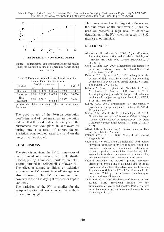
140
Scientific Papers. Series E. Land Reclamation, Earth Observation & Surveying, Environmental Engineering. Vol. VI, 2017Print ISSN 2285-6064, CD-ROM ISSN 2285-6072, Online ISSN 2393-5138, ISSN-L 2285-6064
Figure 4 . Experimental data (markers) and model results (lines) for evolution in time of oil peroxide values during
heat treatment
Table 2. Parameters of mathematical models and the values of statistical indicators
Studied Model parameters ra RMSDb c0 c1 c2 Daylight 1.18 0.0874 0.0026 0.9920 0.3433 Darkness 1.18 0.0983 0.0005 0.9934 0.0776
Heat treatment 1.18 0.5816 -
0.0052 0.9932 0.4641 apearson correlation coefficient; bthe root mean square deviation The good values of the Pearson correlation coefficient and of root mean square deviation indicate that the models describes very well the phenomena that took place in sunflower oil during time as a result of storage factors. Statistical equations obtained are valid on the range of values studied. CONCLUSIONS The study is inquiring the PV for nine types of cold pressed oils walnut oil, milk thistle, linseed, poppy, hempseed, mustard, pumpkin, sesame, almond and refined oil, sunflower oil. The effect of storage conditions on oxidation expressed as PV versus time of storage was also followed. The PV increase in time, however if the oil is daylight exposed or kept to darkness. The variation of the PV is smaller for the samples kept to darkness, comparative to those exposed to daylight.
The temperature has the highest influence on the oxidization of the sunflower oil, thus the used oil presents a high level of oxidative degradation in the PV which increases to 18.32 meq/kg in 60 minutes. REFERENCES Abramovic, H., Abram, V., 2005. Physico-Chemical
Properties, Composition and Oxidative Stability of Camelina sativa Oil, Food Technol. Biotechnol., 43 (1), 63-70.
Choe, E., Ming B.D., 2006. Mechanisms and factors for edible oil oxidation. Comp. Rev. Food Sci. Food Safety, 5 (4): 169-186.
Drumm, T.D., Spanier, A.M., 1991. Changes in the content of lipid autoxidation and su1fur-containing compounds in cooked beef during storage. J. Agric. Food Chem., 39, 336-343.
Kaleem, A., Aziz, S., Iqtedar, M., Abdullah, R., Aftab, M., Rashid, F., Shakoori, F.R., Naz, S., 2015. Investigating changes and effect of peroxide values in cooking oils subject to light and heat. FUUAST J. Biol., 5(2): 191-196.
Lupea, A.X., 2004. Transformări ale biocompuşilor procesaţi în scop alimentar, Editura CEPUSM, Chişinău, 26-72.
Marina, A.M., Wan Rosli, W.I., Noorhidayah, M., 2013. Quantitative Analysis of Peroxide Value in Virgin Coconut Oil by ATRFTIR Spectroscopy, The Open Conference Proceedings Journal 4, (Suppl-2, M13) 53-56.
AOAC Official Method 965.33 Peroxid Value of Oils and Fats. Titration Method.
CODEX-STAN 210 - 1999. Standard for Named Vegetable Oils.
Ordinul nr. 454/917/22 din 22 noiembrie 2001 pentru aprobarea Normelor cu privire la natura, continutul, originea, fabricarea, ambalarea, etichetarea, marcarea, pastrarea si calitatea uleiurilor vegetale, grasimilor tartinabile - margarine - si a maionezelor, destinate comercializarii pentru consumul uman.
Ordinul ANSVSA nr. 27/2011 privind aprobarea criteriilor microbiologice şi de igienă care se aplică produselor alimentare, altele decât cele menţionate în Regulamentul (CE) nr. 2.073/2005 al Comisiei din 15 noiembrie 2005 privind criteriile microbiologice pentru produsele alimentare.
SR ISO 21527-2, 2009 Microbiology of food and animal feeding stuffs. Horizontal method for the enumeration of yeasts and moulds. Part 2: Colony count technique in products with water activity less than or equal to 0,95.
141
Scientific Papers. Series E. Land Reclamation, Earth Observation & Surveying, Environmental Engineering. Vol. VI, 2017Print ISSN 2285-6064, CD-ROM ISSN 2285-6072, Online ISSN 2393-5138, ISSN-L 2285-6064
Figure 4 . Experimental data (markers) and model results (lines) for evolution in time of oil peroxide values during
heat treatment
Table 2. Parameters of mathematical models and the values of statistical indicators
Studied Model parameters ra RMSDb c0 c1 c2 Daylight 1.18 0.0874 0.0026 0.9920 0.3433 Darkness 1.18 0.0983 0.0005 0.9934 0.0776
Heat treatment 1.18 0.5816 -
0.0052 0.9932 0.4641 apearson correlation coefficient; bthe root mean square deviation The good values of the Pearson correlation coefficient and of root mean square deviation indicate that the models describes very well the phenomena that took place in sunflower oil during time as a result of storage factors. Statistical equations obtained are valid on the range of values studied. CONCLUSIONS The study is inquiring the PV for nine types of cold pressed oils walnut oil, milk thistle, linseed, poppy, hempseed, mustard, pumpkin, sesame, almond and refined oil, sunflower oil. The effect of storage conditions on oxidation expressed as PV versus time of storage was also followed. The PV increase in time, however if the oil is daylight exposed or kept to darkness. The variation of the PV is smaller for the samples kept to darkness, comparative to those exposed to daylight.
The temperature has the highest influence on the oxidization of the sunflower oil, thus the used oil presents a high level of oxidative degradation in the PV which increases to 18.32 meq/kg in 60 minutes. REFERENCES Abramovic, H., Abram, V., 2005. Physico-Chemical
Properties, Composition and Oxidative Stability of Camelina sativa Oil, Food Technol. Biotechnol., 43 (1), 63-70.
Choe, E., Ming B.D., 2006. Mechanisms and factors for edible oil oxidation. Comp. Rev. Food Sci. Food Safety, 5 (4): 169-186.
Drumm, T.D., Spanier, A.M., 1991. Changes in the content of lipid autoxidation and su1fur-containing compounds in cooked beef during storage. J. Agric. Food Chem., 39, 336-343.
Kaleem, A., Aziz, S., Iqtedar, M., Abdullah, R., Aftab, M., Rashid, F., Shakoori, F.R., Naz, S., 2015. Investigating changes and effect of peroxide values in cooking oils subject to light and heat. FUUAST J. Biol., 5(2): 191-196.
Lupea, A.X., 2004. Transformări ale biocompuşilor procesaţi în scop alimentar, Editura CEPUSM, Chişinău, 26-72.
Marina, A.M., Wan Rosli, W.I., Noorhidayah, M., 2013. Quantitative Analysis of Peroxide Value in Virgin Coconut Oil by ATRFTIR Spectroscopy, The Open Conference Proceedings Journal 4, (Suppl-2, M13) 53-56.
AOAC Official Method 965.33 Peroxid Value of Oils and Fats. Titration Method.
CODEX-STAN 210 - 1999. Standard for Named Vegetable Oils.
Ordinul nr. 454/917/22 din 22 noiembrie 2001 pentru aprobarea Normelor cu privire la natura, continutul, originea, fabricarea, ambalarea, etichetarea, marcarea, pastrarea si calitatea uleiurilor vegetale, grasimilor tartinabile - margarine - si a maionezelor, destinate comercializarii pentru consumul uman.
Ordinul ANSVSA nr. 27/2011 privind aprobarea criteriilor microbiologice şi de igienă care se aplică produselor alimentare, altele decât cele menţionate în Regulamentul (CE) nr. 2.073/2005 al Comisiei din 15 noiembrie 2005 privind criteriile microbiologice pentru produsele alimentare.
SR ISO 21527-2, 2009 Microbiology of food and animal feeding stuffs. Horizontal method for the enumeration of yeasts and moulds. Part 2: Colony count technique in products with water activity less than or equal to 0,95.
GEOGRAPHICAL INFORMATION SYSTEMS IN DETERMINATION OF SPATIAL FACTORS IN CUTANEOUS LEISHMANIASIS CASES
DISTRIBUTION, IN ADANA, TURKEY
Ozan ARTUN, Hakan KAVUR
Cukurova University,Vocational School of Karaisalı, 01770 Adana, Turkey
Corresponding author email: [email protected]
Abstract In Turkey, metropolitan municipalities are responsible for the insecticide spraying activities in all districts of the cities. Therefore, insecticide spraying is applied in the center of Adana, in the control of vector arthropods and other pests, especially against the sand flies and mosquitoes. In this study, we generated cutaneous leishmaniasis (CL) prediction risk maps based on MODIS and NON-MODIS dataset. Firstly, we determined relationship, between the presence of CL patients, human population, insecticide spraying density and several environmental variables [Enhanced Vegetation Index (EVI), Normalized Difference Vegetation Index (NDVI), Digital Elevation Model (DEM), Day Time Mean LST and Night Time Mean LST] obtained from satellite images of randomly selected 103 points were located in the central districts of Adana province, by univariate and binary logistic regression in PASW. (MoH 2016). ARCMAP 10.2. Software was used for geographical adjustments, creating a database and estimating risk models by using several geographical data. The results emphasize that distribution and the presence of the CL cases were found correlated with human population, insecticide, NDVI (LANDSAT), Day time Mean LST and Night Time Mean LST (MODIS). By using Geographic Information System (GIS) Technologies, the predictions that based on univariate and bivariate binary regression analysis of variables as human population density and insecticide spraying density related to the distribution of CL cases was made. The results were used to produce the prediction maps and the potential distribution areas of the incriminated CL cases with the use of GIS technologies which allowed the identification of the CL risk levels that may provide useful information to guide the control program interventions. Key words: Adana, cutaneous, GIS, insecticide, Leishmaniasis INTRODUCTION Leishmaniasis is a vector-borne diseases, is transmitted by bite of vector sand flies abscess to humans prevalence and the publishing of the disease influenced by economic-social and cultural issues, and especially environmental conditions and natural disasters (WHO, 2010; Yazdanpanah and Rostamianpur, 2013). It is space represented in two clinical types: cutaneous and visceral leishmaniasis caused by several space Leishmania species in Turkey (Ok et al., 2002; Kavur, 2015). The study area is located in Turkey at the Adana province. The collected data of human population, insecticide spraying density and CL patient numbers, has significant features as; suitable temperature, humidity values and flora contents for the sustentation of a vector population and the presence of potential Leishmania endemic infection areas (Alptekinet al., 1999; Volf et al., 2002; Yaman
and Ozbel, 2004; Toprak and Ozer, 2005; Simsek et al., 2007; Svobodova et al., 2009; Tok et al., 2009). These factors has been reported to assist the emergence of CL in the area and a total of 1980 CL patients were diagnosed in 2008 and 2015 in Adana, respectively (MMA, 2015; MoH, 2016). The prevalence and development of leishmaniasis are largely dependent on environmental factors and natural conditions. In addition to the economic, social and cultural conditions, prevalence of leishmaniasis is influenced by ecological factors too. Especially, leishmaniasis incidence has a significant correlation with the values of mean of monthly temperature, the maximum temperature, maximum temperature of monthly (Yazdanpanah and Rostamianpur, 2013). Geographic Information System (GIS) is a system developed to capture, store, manipulate, analyse, manage, and present all types of spatial or geographical data that have associated with them (Glass, 2001). Such as,
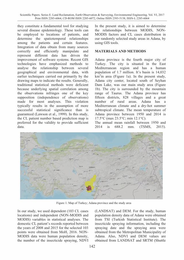
142
Scientific Papers. Series E. Land Reclamation, Earth Observation & Surveying, Environmental Engineering. Vol. VI, 2017Print ISSN 2285-6064, CD-ROM ISSN 2285-6072, Online ISSN 2393-5138, ISSN-L 2285-6064
they constitute a fundamental tool for studying several disease epidemiology. These tools can be employed to locations of patients, and determine the spatiotemporal relationships among the patients and certain features. Integration of data obtain from many sources correctly and efficiently manipulate and represent different data has driven the improvement of software systems. Recent GIS technologies have emphasized methods to analyse the relationship between several geographical and environmental data, with earlier techniques carried out primarily by the drawing maps to indicate the results. Generally, traditional statistical methods were deficient because underlying spatial correlation among the observations infringes one of the key supposition (independence of observations) made for most analyses. This violation typically results in the assumption of more successful statistical significance than is guaranteed (Lawson et al., 1999). In this study, the CL patient number based prediction map is preferred for the validity to provide sufficient data.
In the present study, it is aimed to determine the relationships between MODIS, NON-MODIS factors and CL cases distribution in our randomly selected study areas in Adana, by using GIS tools. MATERIALS AND METHODS Adana province is the fourth major city of Turkey. The city is situated in the East Mediterranean region and has a human population of 1.7 million. It’s basin is 14,032 km2in area (Figure 1a). In the present study, Adana city center, located south of Seyhan Dam Lake, was our main study area (Figure 1b). The city is surrounded by the mountain range of Taurus. The Adana province has fifteen districts, 828 villages and a great number of rural areas. Adana has a Mediterranean climate and a dry-hot summer subtropical climate. The mean temperature of Adana province between 1950 and 2014 is 17.5°C (max 23.5°C; min 12.1°C). The annual mean rainfall between 1950 and 2014 is 688.2 mm. (TSMS, 2015).
Figure 1. Map of Turkey; Adana province and the study area
In our study, we used dependent (103 CL cases locations) and independent (NON-MODIS and MODIS) variables in statistical analyses. The domestic CL patient’s records reported between the years of 2008 and 2015 for the selected 103 points were obtained from MoH, 2016. NON-MODIS data were human population density, the number of the insecticide spraying, NDVI
(LANDSAT) and DEM. For the study, human population density data of Adana were obtained from TSI (Turkish Statistical Institute). The insecticide spraying information, including the spraying date and the spraying area were obtained from the Metropolitan Municipality of Adana. Also, NDVI and DEM values are obtained from LANDSAT and SRTM (Shuttle
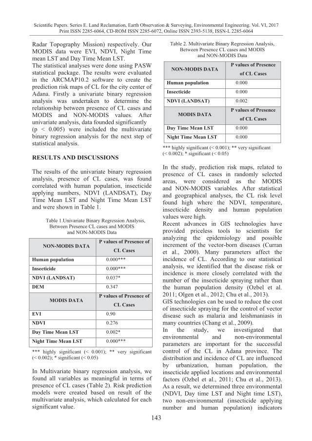
143
Scientific Papers. Series E. Land Reclamation, Earth Observation & Surveying, Environmental Engineering. Vol. VI, 2017Print ISSN 2285-6064, CD-ROM ISSN 2285-6072, Online ISSN 2393-5138, ISSN-L 2285-6064
Radar Topography Mission) respectively. Our MODIS data were EVI, NDVI, Night Time mean LST and Day Time Mean LST. The statistical analyses were done using PASW statistical package. The results were evaluated in the ARCMAP10.2 software to create the prediction risk maps of CL for the city center of Adana. Firstly a univariate binary regression analysis was undertaken to determine the relationship between presence of CL cases and MODIS and NON-MODIS values. After univariate analysis, data founded significantly (p < 0.005) were included the multivariate binary regression analysis for the next step of statistical analysis. RESULTS AND DISCUSSIONS The results of the univariate binary regression analysis, presence of CL cases, was found correlated with human population, insecticide applying numbers, NDVI (LANDSAT), Day Time Mean LST and Night Time Mean LST and were shown in Table 1.
Table 1.Univariate Binary Regression Analysis, Between Presence CL cases and MODIS
and NON-MODIS Data
NON-MODIS DATA P values of Presence of
CL Cases
Human population 0.000***
Insecticide 0.000***
NDVI (LANDSAT) 0.037*
DEM 0.347
MODIS DATA P values of Presence of
CL Cases
EVI 0.90
NDVI 0.276
Day Time Mean LST 0.002*
Night Time Mean LST 0.000***
*** highly significant (< 0.001); ** very significant (< 0.002); * significant (< 0.05)
In Multivariate binary regression analysis, we found all variables as meaningful in terms of presence of CL cases (Table 2). Risk prediction models were created based on result of the multivariate analysis, which calculated for each significant value.
Table 2. Multivariate Binary Regression Analysis, Between Presence CL cases and MODIS
and NON-MODIS Data
NON-MODIS DATA P values of Presence
of CL Cases
Human population 0.000
Insecticide 0.000
NDVI (LANDSAT) 0.002
MODIS DATA P values of Presence
of CL Cases
Day Time Mean LST 0.000
Night Time Mean LST 0.000
*** highly significant (< 0.001); ** very significant (< 0.002); * significant (< 0.05) In the study, prediction risk maps, related to presence of CL cases in randomly selected areas, were considered as the MODIS and NON-MODIS variables. After statistical and geographical analyses, the CL risk level found high where the NDVI, temperature, insecticide density and human population values were high. Recent advances in GIS technologies have provided priceless tools to scientists for analyzing the epidemiology and possible increment of the vector-born diseases (Curran et al., 2000). Many parameters affect the incidence of CL. According to our statistical analysis, we identified that the disease risk or incidence is more closely correlated with the number of the insecticide spraying rather than the human population density (Ozbel et al. 2011; Olgen et al., 2012; Chu et al., 2013). GIS technologies can be used to reduce the cost of insecticide spraying for the control of vector disease such as malaria and leishmaniasis in many countries (Chang et al., 2009). In the study, we investigated that environmental and non-environmental parameters are important for the successful control of the CL in Adana province. The distribution and incidence of CL are influenced by urbanization, human population, the insecticide applied locations and environmental factors (Ozbel et al., 2011; Chu et al., 2013). As a result, we determined three environmental (NDVI, Day time LST and Night time LST), two non-environmental (insecticide applying number and human population) indicators
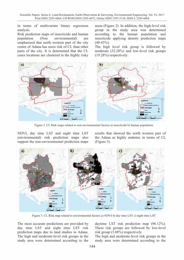
144
Scientific Papers. Series E. Land Reclamation, Earth Observation & Surveying, Environmental Engineering. Vol. VI, 2017Print ISSN 2285-6064, CD-ROM ISSN 2285-6072, Online ISSN 2393-5138, ISSN-L 2285-6064
in terms of multivariate binary regression analysis. Risk prediction maps of insecticide and human population (Non environmental) are emphasized that north western part of the city center of Adana has more risk of CL than other parts of the city. It is determined that the CL cases locations are clustered in the highly risky
areas (Figure 2). In addition, the high-level risk group in the study area was determined according to the human population and insecticide applying density prediction maps (48.43%). The high level risk group is followed by moderate (32.28%) and low-level risk groups (19.28%) respectively.
Figure 2. CL Risk maps related to non-environmental factors a) insecticide b) human population
NDVI, day time LST and night time LST (environmental) risk prediction maps also support the non-environmental prediction maps
results that showed the north western part of the Adana as highly endemic in terms of CL (Figure 3).
Figure 3. CL Risk map related to environmental factors a) NDVI b) day time LST c) night time LST
The most accurate predictions are provided by day time LST and night time LST risk prediction maps due to land studies in Adana. The high and moderate-level risk groups in the study area were determined according to the
daytime LST risk prediction map (96.12%). These risk groups are followed by low-level risk group (3.88%) respectively. The high and moderate-level risk groups in the study area were determined according to the
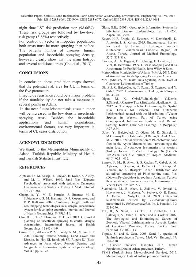
145
Scientific Papers. Series E. Land Reclamation, Earth Observation & Surveying, Environmental Engineering. Vol. VI, 2017Print ISSN 2285-6064, CD-ROM ISSN 2285-6072, Online ISSN 2393-5138, ISSN-L 2285-6064
night time LST risk prediction map (98.06%). These risk groups are followed by low-level risk group (3.88%) respectively. For control of vector arthropodes population, both areas must be more spraying than before. The patients number of diseases, human population and insecticide spraying density, however, clearly show that the main hotspot and several additional areas (Chu et al., 2013). CONCLUSIONS In conclusion, these prediction maps showed that the potential risk area for CL in terms of the five parameters. Insecticide resistance could be a major problem if the municipality did not take a measure in several points in Adana. In the near future leishmaniasis cases number will be increased in the low density insecticide spraying areas. Besides the insecticide applications and human populations, environmental factors, are very important in terms of CL cases distribution.
ACKNOWLEDGMENTS
We thank to the Metropolitan Municipality of Adana, Turkish Republic Ministry of Health and Turkish Statistical Institute. REFERENCES
Alptekin, D., M. Kasap, U. Luleyap, H. Kasap, S. Aksoy,
and M. L. Wilson. 1999. Sand flies (Diptera: Psychodidae) associated with epidemic Cutaneous Leishmaniasis in Sanlıurfa. Turkey. J. Med. Entomol. 36: 277–281.
Chang, A. Y., M. E. Parrales, J. Jimenez, M. E. Sobieszczyk, S. M. Hammer, D. J. Copenhaver, and R. P. Kulkarni. 2009. Combining Google Earth and GIS mapping technologies in a dengue surveillance system for developing countries. International Journal of Health Geographics. 8 (49):1-11.
Chu, H. J., T. C. Chan, and F. J. Jao. 2013. GIS-aided planning of insecticide spraying to control dengue transmission. International Journal of Health Geographics. 12 (42): 1-9.
Curran P. J., Atkinson P. M., Foody G. M., Milton E. J: 2000. Linking Remote Sensing, Land Cover and Disease. In, Hay SI, Randolph SE, Rogers DJ (Eds): Advances in Parasitology: Remote Sensing and Geographical Information Systems in Epidemiology. Vol. 47, pp. 37-72.
Glass, G.E., (2001). Geographic Information Systems In Infectious Disease Epidemiology. pp. 231–253, Aspen Publishers.
Kavur, H.,F. Eroglu, G. Evyapan, M. Demirkazik, D. Alptekin, I. S. Koltas. 2015. Entomological Survey for Sand Fly Fauna in Imamoglu Province (Cutaneous Leishmaniasis Endemic Region) of Adana, Turkey. Journal of Medical Entomology. 52(5):813-818.
Lawson, A.; A. Biggeri, D. Bohning, E. Lesaffre, J. F. Viel, R. Bertollini. 1999. Disease Mapping and Risk Assessment for Public Health. John Wiley & Sons.
Metropolitan Municipality of Adana (MMA), 2015. Data of Annual Insecticide Spraying Density in Adana.
MoH (Ministry of Health Data System), 2016. Data of Cutaneous Leishmaniasis of Turkey.
Ok, Z.,I. C. Balcıoğlu, A. T. Ozkan, S. Ozensoy, and Y. Ozbel. 2002. Leishmaniasis in Turkey, ActaTropica, 84: 43-48.
Olgen, M. K., Ozbel,Y..Balcioglu,I. C.Demir, S.Simsek,F.OzensoyToz,S.Ertabaklar,H.Alkan.M. Z. 2012. A New Approach for Determining the Spatial Risk Levels for Visceral and Cutaneous Leishmaniasis related with the Distribution of Vector Species in Western Part of Turkey using Geographical Information Systems and Remote Sensing. Kafkas Univ Vet FakDerg. 18 (Suppl-A): A77-A84.
Ozbel, Y., Balcioglu,I. C. Olgen, M. K. Simsek, F. M.OzensoyToz,S.Ertabaklar,H.Demir,S. And Alkan. M. Z. 2011. Spatial distribution of Phlebotomine sand flies in the Aydin Mountains and surroundings: the main focus of cutaneous leishmaniasis in western Turkey. Journal of Vector Ecology. 36 (1): 99-105.Asian Paci fi c Journal of Tropical Medicine. 9(10): 925 – 932.
Simsek, F. M., B. Alten, S. S. Caglar, Y. Ozbel, A. M. Aytekin, S. Kaynas, A. Belen, O. E. Kasap, M. Yaman, and S. Rastgeldi. 2007. Distribution and altitudinal structuring of Phlebotomine sand flies (Diptera:Psychodidae) in southern Anatolia, Turkey: their relation to human cutaneous leishmaniasis. J. Vector Ecol. 32: 269–279.
Svobodova, M., B. Alten, L. Zidkova, V. Dvorak, J. Hlavackova, J. Myskova, V. Seblova, O. E. Kasap, A. Belen, J. Votypka, et al. 2009. Cutaneous leishmaniasis caused by Leishmaniainfantum transmitted by Phlebotomustobbi. Int. J. Parasitol. 39: 251–256.
Tok, H., N. Sevil, S. O. Toz, H. Ertabaklar, I. C. Balcıoglu, S. Demir, Y. Ozbel, and A. Coskun. 2009. The Serological and Entomological Survey of Zoonotic Visceral Leishmaniasis in Ayvacik Region of Canakkale Province, Turkey. Turkish Soc. Parasitol. 33: 109–113.
Toprak, S., and N. Ozer. 2005. Sand fly species of Sanlıurfa province in Turkey. Med. Vet. Entomol. 19: 107–110.
TSI (Turkish Statistical Institute), 2015. Human Population Data of Adana province, Turkey.
TSMS (Turkish State Meteorological Service), 2015. Meteorological Data of Adana province, Turkey.

146
Scientific Papers. Series E. Land Reclamation, Earth Observation & Surveying, Environmental Engineering. Vol. VI, 2017Print ISSN 2285-6064, CD-ROM ISSN 2285-6072, Online ISSN 2393-5138, ISSN-L 2285-6064
WHO (World Health Organization). 2010. WHO Technical Report Series Report No: 949.
Volf, P., Y. Ozbel, F. Akkafa, M. Svobodova, J. Votypka, and K. P. Chang. 2002. Sand Flies (Diptera: Phlebotominae) in Sanliurfa, Turkey: Relationship of Phlebotomussergenti with the Epidemic of Anthroponotic Cutaneous Leishmaniasis. J. Med. Entomol. 39: 12–15.
Yaman, M., and Y. Ozbel. 2004. The sand flies (Diptera: Psychodidae) in the Turkish province of Hatay: some possible vectors of the parasites causing human cutaneous leishmaniasis. Ann. Trop. Med. Parasitol. 98: 741–750.
Yazdanpanah, H. A., Rostamianpur, M. 2013. Analysis of Spatial Distribution of Leishmaniasis and its Relationship with Climatic Parameters (Case Study: Ilam Province). BEPLS 2: 80-86
147
Scientific Papers. Series E. Land Reclamation, Earth Observation & Surveying, Environmental Engineering. Vol. VI, 2017Print ISSN 2285-6064, CD-ROM ISSN 2285-6072, Online ISSN 2393-5138, ISSN-L 2285-6064
WHO (World Health Organization). 2010. WHO Technical Report Series Report No: 949.
Volf, P., Y. Ozbel, F. Akkafa, M. Svobodova, J. Votypka, and K. P. Chang. 2002. Sand Flies (Diptera: Phlebotominae) in Sanliurfa, Turkey: Relationship of Phlebotomussergenti with the Epidemic of Anthroponotic Cutaneous Leishmaniasis. J. Med. Entomol. 39: 12–15.
Yaman, M., and Y. Ozbel. 2004. The sand flies (Diptera: Psychodidae) in the Turkish province of Hatay: some possible vectors of the parasites causing human cutaneous leishmaniasis. Ann. Trop. Med. Parasitol. 98: 741–750.
Yazdanpanah, H. A., Rostamianpur, M. 2013. Analysis of Spatial Distribution of Leishmaniasis and its Relationship with Climatic Parameters (Case Study: Ilam Province). BEPLS 2: 80-86
IMPORTANCE OF TOPOLOGY IN A GIS PROJECT OF MONITORING
THE SOILS IN AGRICULTURAL LAND
Gabriela BIALI, Paula COJOCARU
“Gheorghe Asachi” Technical University of Iasi, 65 Mangeron Blvd, Iasi, Romania
Corresponding author email: [email protected]
Abstract This paper presents the advantages of using the topology in a GIS project. The study was conducted on two watershed with mainly agricultural uses. We presented a model for creating the topology designed to monitoring the soils in the basins studied. In the present application, we qualify the graphical objects as soil units on the map. After the topology there was possible the grouping in thematic layers depending on their type and on many other information from the attribute-type database (erodability, humus content, texture, structure, pH etc.). Topological relations were created through an own program in Fortran language under Windows). The topological structure of spatial database in this GIS project is under Geo-Graph software. The existence of topology also brings another major advantage of the project: facilitates the creation of key links between databases, the important step towards the query. Key words: database, GIS, layers, soils , topology INTRODUCTION Topology is a mathematical procedure to explicitly define the spatial relations: defining connections between lines, identification of adjacent polygons, defining a polygon as a set (an aggregate) of lines. The spatial relationships between geographic objects of a map are plotted on that map, but their interpretation depends on the person that reads the map. Creating the topology in a GIS makes explicit certain relations between objects. In other words, the topology is a codification of spatial relationships between the objects of a layer that are connected or are adjacent (lines, nodes, polygons). For example, the topology of a line means knowing the start and end points (nodes) and the polygons to the left and right. The generation of topology represents the process of building topological relations between the objects of a layer (Renard K., 1996). Explicit generation of topology may be mandatory after subsequent changes or updates of the graphical database (disconnected topology), or may be implicitly assumed by the software (dynamic topology). As regards the mapping, the relations and functions of graphical elements will always be targeted towards the effectiveness of storage
and the location of spatial elements. In the past, the amount of mapped information and diversity of usable data sources have made it difficult to establish such functions. Separation of spatial elements from their thematic attributes and organizational structure of these ensembles foreshadowed spatial databases used today in GIS. Thus it appeared the topological structure (for storing data in vector model), which is based on adjacency properties and spatial relationships between different elements (objects) of a map. Lack of topological relations in a vector representation, reduces much the query possibilities, even if the user manages to deduce on his own, visually, some of these relationships (Biali G., Popovici N., 2003). The topological model (corresponding to the numerical maps and plans where, not only the data are digitally represented in vector format, but they are also added the topological relations between objects), incorporates for a map or a plan in vector form three sets of data: � Identifiers of characteristics of the land to be plotted in vector map or plan, and which, corresponding to their geometry, are divided in three generic types: point objects, line objects and surface objects;
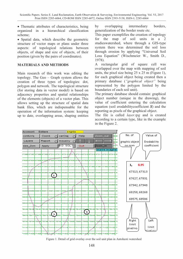
148
Scientific Papers. Series E. Land Reclamation, Earth Observation & Surveying, Environmental Engineering. Vol. VI, 2017Print ISSN 2285-6064, CD-ROM ISSN 2285-6072, Online ISSN 2393-5138, ISSN-L 2285-6064
� Thematic attributes of characteristics, being organized in a hierarchical classification scheme; � Spatial data, which describe the geometric structure of vector maps or plans under three aspects: of topological relations between objects, of shape and size of objects, of their position (given by the pairs of coordinates). MATERIALS AND METHODS Main research of this work was editing the topology. The Geo – Graph system allows the creation of three types of topologies: dot, polygon and network. The topological structure (for storing data in vector model) is based on adjacency properties and spatial relationships of the elements (objects) of a vector plan. This allows setting up the structure of spatial data bank files, which are indispensable for the operation of the information system: keeping up to date, overlapping areas, shaping entities
by overlapping intermediary borders, generalization of the border route etc. This paper exemplifies the creation of topology for the map of soil units in a 2 studieswatershed, where through a GIS-type system there was determined the soil loss through erosion by applying “Universal Soil Loss Equation” (Wischmeier W., Smith D., 1978). A rectangular grid of square cell was overlapped over the map with mapping of soil units, the pixel size being 25 x 25 m (Figure 1), for each graphical object being created then a primary database (“graphical object” being represented by the polygon limited by the boundaries of each soil unit). The primary database should contain: graphical object number (unique in the drawing), the value of coefficient entering the calculation equation (soil erodabilitycoefficient S) and the reporting as pixels of the graphical object. The file is called layer.tpg and is created according to a certain type, like in the example in the Figure 2.
Figure 1. Detail of grid overlay over the soil unit plan in Antohesti watershed
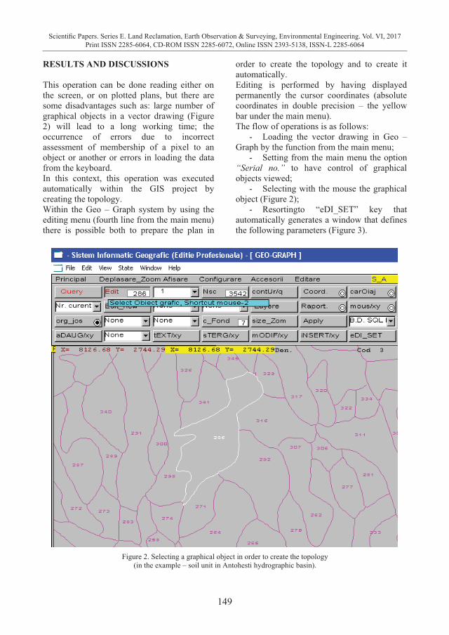
149
Scientific Papers. Series E. Land Reclamation, Earth Observation & Surveying, Environmental Engineering. Vol. VI, 2017Print ISSN 2285-6064, CD-ROM ISSN 2285-6072, Online ISSN 2393-5138, ISSN-L 2285-6064
� Thematic attributes of characteristics, being organized in a hierarchical classification scheme; � Spatial data, which describe the geometric structure of vector maps or plans under three aspects: of topological relations between objects, of shape and size of objects, of their position (given by the pairs of coordinates). MATERIALS AND METHODS Main research of this work was editing the topology. The Geo – Graph system allows the creation of three types of topologies: dot, polygon and network. The topological structure (for storing data in vector model) is based on adjacency properties and spatial relationships of the elements (objects) of a vector plan. This allows setting up the structure of spatial data bank files, which are indispensable for the operation of the information system: keeping up to date, overlapping areas, shaping entities
by overlapping intermediary borders, generalization of the border route etc. This paper exemplifies the creation of topology for the map of soil units in a 2 studieswatershed, where through a GIS-type system there was determined the soil loss through erosion by applying “Universal Soil Loss Equation” (Wischmeier W., Smith D., 1978). A rectangular grid of square cell was overlapped over the map with mapping of soil units, the pixel size being 25 x 25 m (Figure 1), for each graphical object being created then a primary database (“graphical object” being represented by the polygon limited by the boundaries of each soil unit). The primary database should contain: graphical object number (unique in the drawing), the value of coefficient entering the calculation equation (soil erodabilitycoefficient S) and the reporting as pixels of the graphical object. The file is called layer.tpg and is created according to a certain type, like in the example in the Figure 2.
Figure 1. Detail of grid overlay over the soil unit plan in Antohesti watershed
RESULTS AND DISCUSSIONS This operation can be done reading either on the screen, or on plotted plans, but there are some disadvantages such as: large number of graphical objects in a vector drawing (Figure 2) will lead to a long working time; the occurrence of errors due to incorrect assessment of membership of a pixel to an object or another or errors in loading the data from the keyboard. In this context, this operation was executed automatically within the GIS project by creating the topology. Within the Geo – Graph system by using the editing menu (fourth line from the main menu) there is possible both to prepare the plan in
order to create the topology and to create it automatically. Editing is performed by having displayed permanently the cursor coordinates (absolute coordinates in double precision – the yellow bar under the main menu). The flow of operations is as follows:
- Loading the vector drawing in Geo – Graph by the function from the main menu;
- Setting from the main menu the option “Serial no.” to have control of graphical objects viewed;
- Selecting with the mouse the graphical object (Figure 2);
- Resortingto “eDI_SET” key that automatically generates a window that defines the following parameters (Figure 3).
Figure 2. Selecting a graphical object in order to create the topology (in the example – soil unit in Antohesti hydrographic basin).
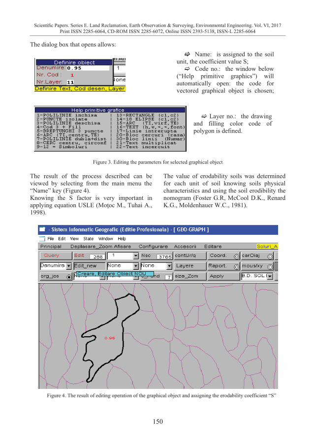
150
Scientific Papers. Series E. Land Reclamation, Earth Observation & Surveying, Environmental Engineering. Vol. VI, 2017Print ISSN 2285-6064, CD-ROM ISSN 2285-6072, Online ISSN 2393-5138, ISSN-L 2285-6064
The dialog box that opens allows:
Figure 3. Editing the parameters for selected graphical object
The result of the process described can be viewed by selecting from the main menu the “Name” key (Figure 4). Knowing the S factor is very important in applying equation USLE (Moţoc M., Tuhai A., 1998).
The value of erodability soils was determined for each unit of soil knowing soils physical characteristics and using the soil erodibility the nomogram (Foster G.R, McCool D.K., Renard K.G., Moldenhauer W.C., 1981).
Figure 4. The result of editing operation of the graphical object and assigning the erodability coefficient “S”
� Name: is assigned to the soil unit, the coefficient value S;
� Code no.: the window below (“Help primitive graphics”) will automatically open: the code for vectored graphical object is chosen;
� Layer no.: the drawing and filling color code of polygon is defined.
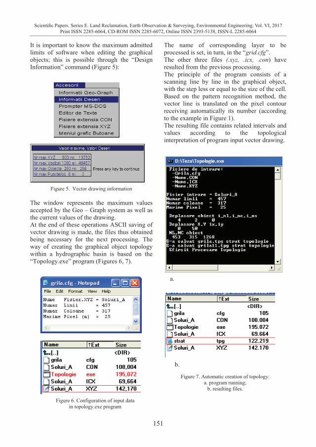
151
Scientific Papers. Series E. Land Reclamation, Earth Observation & Surveying, Environmental Engineering. Vol. VI, 2017Print ISSN 2285-6064, CD-ROM ISSN 2285-6072, Online ISSN 2393-5138, ISSN-L 2285-6064
The dialog box that opens allows:
Figure 3. Editing the parameters for selected graphical object
The result of the process described can be viewed by selecting from the main menu the “Name” key (Figure 4). Knowing the S factor is very important in applying equation USLE (Moţoc M., Tuhai A., 1998).
The value of erodability soils was determined for each unit of soil knowing soils physical characteristics and using the soil erodibility the nomogram (Foster G.R, McCool D.K., Renard K.G., Moldenhauer W.C., 1981).
Figure 4. The result of editing operation of the graphical object and assigning the erodability coefficient “S”
� Name: is assigned to the soil unit, the coefficient value S;
� Code no.: the window below (“Help primitive graphics”) will automatically open: the code for vectored graphical object is chosen;
� Layer no.: the drawing and filling color code of polygon is defined.
It is important to know the maximum admitted limits of software when editing the graphical objects; this is possible through the “Design Information” command (Figure 5):
Figure 5. Vector drawing information
The window represents the maximum values accepted by the Geo – Graph system as well as the current values of the drawing. At the end of these operations ASCII saving of vector drawing is made, the files thus obtained being necessary for the next processing. The way of creating the graphical object topology within a hydrographic basin is based on the “Topology.exe” program (Figures 6, 7).
Figure 6. Configuration of input data in topology.exe program
The name of corresponding layer to be processed is set, in turn, in the “grid.cfg”. The other three files (.xyz, .icx, .con) have resulted from the previous processing. The principle of the program consists of a scanning line by line in the graphical object, with the step less or equal to the size of the cell. Based on the pattern recognition method, the vector line is translated on the pixel contour receiving automatically its number (according to the example in Figure 1). The resulting file contains related intervals and values according to the topological interpretation of program input vector drawing.
Figure 7. Automatic creation of topology: a. program running;
b. resulting files.
b.
a.
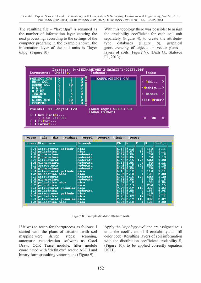
152
Scientific Papers. Series E. Land Reclamation, Earth Observation & Surveying, Environmental Engineering. Vol. VI, 2017Print ISSN 2285-6064, CD-ROM ISSN 2285-6072, Online ISSN 2393-5138, ISSN-L 2285-6064
The resulting file – “layer.tpg” is renamed as the number of information layer entering the next processing, according to the settings of the computer program; in the example shown, the information layer of the soil units is “layer 6.tpg” (Figure 10).
With this topology there was possible: to assign the erodability coefficient for each soil unit separately (Figure 4), to create the attribute-type databases (Figure 8), graphical georeferencing of objects on vector plans – layers of soils (Figure 9), (Biali G., Statescu Fl., 2013).
If it was to recap for shortprocess as follows: I started with the plans of situation with soil mapping;were driven steps: scanning, automatic vectorization software as Corel Draw, OCR Trace module, filter module coordinated with "dxfin.exe" rescue ASCII and binary forms;resulting vector plans (Figure 9).
Apply the "topology.exe" and are assigned soils units the coefficient of S erodabilityand fill color code. Resulting layers of soil information with the distribution coefficient erodability S, (Figure 10), to be applied correctly equation USLE.
Figure 8. Example database attribute soils
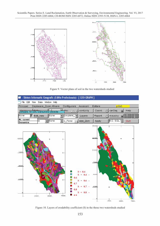
153
Scientific Papers. Series E. Land Reclamation, Earth Observation & Surveying, Environmental Engineering. Vol. VI, 2017Print ISSN 2285-6064, CD-ROM ISSN 2285-6072, Online ISSN 2393-5138, ISSN-L 2285-6064
The resulting file – “layer.tpg” is renamed as the number of information layer entering the next processing, according to the settings of the computer program; in the example shown, the information layer of the soil units is “layer 6.tpg” (Figure 10).
With this topology there was possible: to assign the erodability coefficient for each soil unit separately (Figure 4), to create the attribute-type databases (Figure 8), graphical georeferencing of objects on vector plans – layers of soils (Figure 9), (Biali G., Statescu Fl., 2013).
If it was to recap for shortprocess as follows: I started with the plans of situation with soil mapping;were driven steps: scanning, automatic vectorization software as Corel Draw, OCR Trace module, filter module coordinated with "dxfin.exe" rescue ASCII and binary forms;resulting vector plans (Figure 9).
Apply the "topology.exe" and are assigned soils units the coefficient of S erodabilityand fill color code. Resulting layers of soil information with the distribution coefficient erodability S, (Figure 10), to be applied correctly equation USLE.
Figure 8. Example database attribute soils
Figure 9. Vector plans of soil in the two watersheds studied
Figure 10. Layers of erodability coefficient (S) in the those two watersheds studied
S < 0.4 S = 0.4 –
0.6 S = 0.6 –
0.7 S = 0.7 –
0.8 S = 0.8 –
0 9
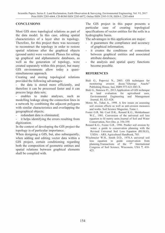
154
Scientific Papers. Series E. Land Reclamation, Earth Observation & Surveying, Environmental Engineering. Vol. VI, 2017Print ISSN 2285-6064, CD-ROM ISSN 2285-6072, Online ISSN 2393-5138, ISSN-L 2285-6064
CONCLUSIONS Most GIS store topological relations as part of the data model. In this case, editing spatial characteristics of a layer alter its topology. Therefore, for this project there was necessary to reconstruct the topology in order to restore spatial relations after the graphical objects (ground units) were vectored. Phases for setting up graphical and alphanumeric databases, as well as the generation of topology, were created separately within this project, but many GIS environments allow today a quasi-simultaneous approach. Creating and storing topological relations provided the following advantages: - the data is stored more efficiently, and therefore it can be processed faster and it can process large data sets; - enables to make analyses, such as modelling leakage along the connection lines in a network by combining the adjacent polygons with similar characteristics and overlapping the geographical objects; - redundant data is eliminated; - it helps identifying the errors resulting from digitization. In the context of developing the GIS project the topology is of particular importance. When designing a GIS, but, also subsequently, when adding and editing vector data within a GIS project, certain conditioning regarding both the composition of geometric entities and spatial relations between graphical elements shall be complied with.
The GIS project in this paper presents a particular case of creating topological specifications of vector entities for the soils in a hydrographic basin. The advantages in this application are major: - it guarantees the compliance and accuracy
of graphical information; - it creates the conditions of connection
between graphical entities and associated attribute databases;
- the analysis and spatial query functions become possible.
REFERENCES Biali G., Popovici N., 2003. GIS techniques for
monitoring erosion decay.”Gheorge Asachi” Publishing House, Iasi, ISBN 973-621-043-X.
Biali G., Statescu Fl., 2013.Application of GIS technique in land evaluation for agricultural uses, Environmental Engineering and Management Journal, 11, 821-828.
Motoc M., Tuhai A., 1998. A few issues on assessing soil erosion effects as well as anti-erosion measures and works. Soil Science Magazine, Tome.1.
Foster G.R, Mc Cool D.K., Renard K.G., Moldenhauer W.C., 1981. Conversion of the universal soil loss equation to SI metric units.Journal of Soil and Water Conservation, Nov-Dec. p. 356-359.
Renard K.G., Foster G.R., 1996. Predict soil erosion by water: a guide to conservation planning with the Revised Universal Soil Loss Equation (RUSLE), USDA – ARS, Agricultural Handbook, 703.
Wischmeier W.H., Smith D.D., 1978.A universal soil loss equation to guide conservation from planning,Transactions of the 7th International Congress of Soil Science, Wisconsin, USA 7, 418-425.
155
Scientific Papers. Series E. Land Reclamation, Earth Observation & Surveying, Environmental Engineering. Vol. VI, 2017Print ISSN 2285-6064, CD-ROM ISSN 2285-6072, Online ISSN 2393-5138, ISSN-L 2285-6064
CONCLUSIONS Most GIS store topological relations as part of the data model. In this case, editing spatial characteristics of a layer alter its topology. Therefore, for this project there was necessary to reconstruct the topology in order to restore spatial relations after the graphical objects (ground units) were vectored. Phases for setting up graphical and alphanumeric databases, as well as the generation of topology, were created separately within this project, but many GIS environments allow today a quasi-simultaneous approach. Creating and storing topological relations provided the following advantages: - the data is stored more efficiently, and therefore it can be processed faster and it can process large data sets; - enables to make analyses, such as modelling leakage along the connection lines in a network by combining the adjacent polygons with similar characteristics and overlapping the geographical objects; - redundant data is eliminated; - it helps identifying the errors resulting from digitization. In the context of developing the GIS project the topology is of particular importance. When designing a GIS, but, also subsequently, when adding and editing vector data within a GIS project, certain conditioning regarding both the composition of geometric entities and spatial relations between graphical elements shall be complied with.
The GIS project in this paper presents a particular case of creating topological specifications of vector entities for the soils in a hydrographic basin. The advantages in this application are major: - it guarantees the compliance and accuracy
of graphical information; - it creates the conditions of connection
between graphical entities and associated attribute databases;
- the analysis and spatial query functions become possible.
REFERENCES Biali G., Popovici N., 2003. GIS techniques for
monitoring erosion decay.”Gheorge Asachi” Publishing House, Iasi, ISBN 973-621-043-X.
Biali G., Statescu Fl., 2013.Application of GIS technique in land evaluation for agricultural uses, Environmental Engineering and Management Journal, 11, 821-828.
Motoc M., Tuhai A., 1998. A few issues on assessing soil erosion effects as well as anti-erosion measures and works. Soil Science Magazine, Tome.1.
Foster G.R, Mc Cool D.K., Renard K.G., Moldenhauer W.C., 1981. Conversion of the universal soil loss equation to SI metric units.Journal of Soil and Water Conservation, Nov-Dec. p. 356-359.
Renard K.G., Foster G.R., 1996. Predict soil erosion by water: a guide to conservation planning with the Revised Universal Soil Loss Equation (RUSLE), USDA – ARS, Agricultural Handbook, 703.
Wischmeier W.H., Smith D.D., 1978.A universal soil loss equation to guide conservation from planning,Transactions of the 7th International Congress of Soil Science, Wisconsin, USA 7, 418-425.
MAIN FRAMEWORK AND INDICATORS USED IN MAPPING AND ASSESSMENT OF ECOSYSTEM SERVICES FOR THE EU
BIODIVERSITY STRATEGY UP TO 2020
Cristina BURGHILA, Sorin Mihai CIMPEANU, Alexandru BADEA
University of Agronomic Sciences and Veterinary Medicine of Bucharest, 59 Marasti Blvd, District 1, Bucharest, Romania
Corresponding author email: [email protected]
Abstract Pollution, over exploitations, urban development and climate changes cause huge losses on our natural capital. The human race depends on healthy ecosystems to deliver essential services such as food, water, clean air and recreation. The need of quantifying the levels and values of these ecosystems services and incorporate them into resource management is increasing each and every day. According to EU biodiversity strategy up to 2020 (EC 2011), target 2, by 2020 ecosystems and their services must be maintained and enhanced by restoring at least 15% of degraded ecosystems. In order to measure the progress towards this target, is essential to map ecosystems and their condition. At EU and national level is proposed a general and analytical framework based on the DPSIR framework (Drivers, Pressures, State, Impact and Response) in order to integrate economic values into accounting and reporting system, but also to provide cross references with ecosystem services categories that are being used in assessments. The big challenge that European Commission is facing consists in using the large amount of geospatial data and other information that are available for building a feasible methodology and suitable data sets. The framework to be used is developed by CICES and it was evaluated among 4 pilot studies of MAES working group, same working group that came along with the proposal of indicators for mapping and assessing urban ecosystems and their services applicable to EU and most of its Member States. MAES outcome of the working group showed that when using data that already exist and combine it in a coherent and integrated ecosystem assessment yields a starting database consistency. Key words: biodiversity, ecosystem services, framework, indicators, MAES INTRODUCTION In 2011 was adopted, by the European Commission and Council, the EU Biodiversity Strategy for 2020. The main goal up to 2020 is, on the one hand, to stop the loss of biodiversity and the degradation of ecosystem services and, on the other hand, to restore them as far as feasible in the EU and its Member States. The EU Biodiversity Strategy includes among its components 6 interdependent targets and 20 supporting actions. Inside of Target 2, there is an action that calls for restoration of ecosystems and their services called Action 5. Within it, Member States, with the help of the Commission, are called to map and asses the state of ecosystems and the value of their services promoting the integration of those values into accounting and reporting systems at EU and national scale. The implementation of
Action 5 is supervised by the working group on Mapping and Assessment of Ecosystem and their Services (MAES). The MAES structure facilitates the collaboration between EU bodies, EC’s experts, member states, stakeholder’s representatives and NGOs and takes part into supporting actions such as Commission’s research and reports. The prior objectives of the MAES project are: 1. Protect and enhance natural capital
(biodiversity, land and soil, water and marine, forests, nutrient cycle);
2. Facilitate the transition to resource efficient, low-carbon economy (climate mitigation, eco innovation, industrial emission, water stress;
3. Safeguard health & well-being (air quality, chemicals, climate adaptation, drinking and bathing water quality, noise).
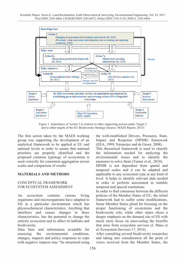
156
Scientific Papers. Series E. Land Reclamation, Earth Observation & Surveying, Environmental Engineering. Vol. VI, 2017Print ISSN 2285-6064, CD-ROM ISSN 2285-6072, Online ISSN 2393-5138, ISSN-L 2285-6064
Figure 1. Importance of Action 5 in relation to other supporting actions under Target 2 and to other targets of the EU Biodiversity Strategy (Source: MAES Report, 2013)
The first action taken by the MAES working group was supporting the development of an analytical framework to be applied at EU and national levels in order to assure that national priorities are properly identified and the proposed common typology of ecosystems is used correctly for consistent aggregation across scales and comparison of results MATERIALS AND METHODS CONCEPTUAL FRAMEWORK FOR ECOSYSTEM ASSESSMENT An ecosystem contains various living organisms and microorganisms have adapted to life in a particular environment which has physicochemical characteristics. Anything that interferes and causes changes to these characteristics, has the potential to change the entirely ecosystem and to affect its habitats and biodiversity. Data base and information available for assessing the environmental conditions, changes, impacts and policy responses to cope with negative impacts may “be structured using
the well-established Drivers, Pressures, State, Impact and Response (DPSIR) framework (EEA, 1999; Niemeijer and de Groot, 2008). This theoretical framework is used to classify the information needed for analyzing the environmental issues and to identify the measures to solve them (Turner et al., 2010). DPSIR is not dependent from spatial and temporal scales and it can be adapted and applicable to any ecosystem type at any kind of level. It helps to identify relevant data needed in order to perform assessment in suitable temporal and special resolutions. In order to find consensus between the different policies of the Member States of EU, the initial framework had to suffer some modifications. Some Member States plead for focusing on the proper functioning of ecosystems and the biodiversity role, while other states chose a deeper emphasis on the demand site of ES with much more focus on unrevealing the benefits that arise from ecosystem services (J. Maes et al./Ecosystem Services 17, 2016). After consulting several biodiversity researches and taking into consideration all the point of views received from the Member States, the
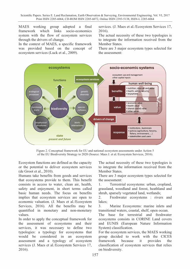
157
Scientific Papers. Series E. Land Reclamation, Earth Observation & Surveying, Environmental Engineering. Vol. VI, 2017Print ISSN 2285-6064, CD-ROM ISSN 2285-6072, Online ISSN 2393-5138, ISSN-L 2285-6064
Figure 1. Importance of Action 5 in relation to other supporting actions under Target 2 and to other targets of the EU Biodiversity Strategy (Source: MAES Report, 2013)
The first action taken by the MAES working group was supporting the development of an analytical framework to be applied at EU and national levels in order to assure that national priorities are properly identified and the proposed common typology of ecosystems is used correctly for consistent aggregation across scales and comparison of results MATERIALS AND METHODS CONCEPTUAL FRAMEWORK FOR ECOSYSTEM ASSESSMENT An ecosystem contains various living organisms and microorganisms have adapted to life in a particular environment which has physicochemical characteristics. Anything that interferes and causes changes to these characteristics, has the potential to change the entirely ecosystem and to affect its habitats and biodiversity. Data base and information available for assessing the environmental conditions, changes, impacts and policy responses to cope with negative impacts may “be structured using
the well-established Drivers, Pressures, State, Impact and Response (DPSIR) framework (EEA, 1999; Niemeijer and de Groot, 2008). This theoretical framework is used to classify the information needed for analyzing the environmental issues and to identify the measures to solve them (Turner et al., 2010). DPSIR is not dependent from spatial and temporal scales and it can be adapted and applicable to any ecosystem type at any kind of level. It helps to identify relevant data needed in order to perform assessment in suitable temporal and special resolutions. In order to find consensus between the different policies of the Member States of EU, the initial framework had to suffer some modifications. Some Member States plead for focusing on the proper functioning of ecosystems and the biodiversity role, while other states chose a deeper emphasis on the demand site of ES with much more focus on unrevealing the benefits that arise from ecosystem services (J. Maes et al./Ecosystem Services 17, 2016). After consulting several biodiversity researches and taking into consideration all the point of views received from the Member States, the
MAES working group adopted a final framework which links socio-economics system with the flow of ecosystem services through the drivers of change. In the context of MAES, a specific framework was provided based on the concept of ecosystem services (Luck et al., 2009).
services. (J. Maes et al./Ecosystem Services 17, 2016). The actual necessity of these two typologies is to integrate the information received from the Member States. There are 3 major ecosystem types selected for the assessment:
Figure 2. Conceptual framework for EU and national ecosystem assessments under Action 5 of the EU Biodiversity Strategy to 2020 (Source: Maes J. et al./Ecosystem Services, 2016).
Ecosystem functions are defined as the capacity or the potential to deliver ecosystem services (de Groot et al., 2010). Humans take benefits from goods and services that ecosystems provide to them. This benefit consists in access to water, clean air, health, safety and enjoyment, in short terms called basic human needs. The focus on benefits implies that ecosystem services are open to economic valuation. (J. Maes et al./Ecosystem Services, 2016). All the benefits may be quantified in monetary and non-monetary values. In order to apply the conceptual framework for the assessment of ecosystems and their services, it was necessary to define two typologies: a typology for ecosystems that would be considered in an ecosystem assessment and a typology of ecosystem services (J. Maes et al./Ecosystem Services 17, 2016).
The actual necessity of these two typologies is to integrate the information received from the Member States. There are 3 major ecosystem types selected for the assessment: 1. Terrestrial ecosystems: urban, cropland, grassland, woodland and forest, heathland and shrub, sparsely vegetated land, wetlands; 2. Freshwater ecosystems : rivers and lakes; 3. Marine Ecosystems: marine inlets and transitional waters, coastal, shelf, open ocean. The base for terrestrial and freshwater ecosystems consists in CORINE Land covers and EUNIS (European Nature Information System) classification. For the ecosystem services, the MAES working group decided to work with the CICES framework because it provides the classification of ecosystem services that relies on biodiversity.
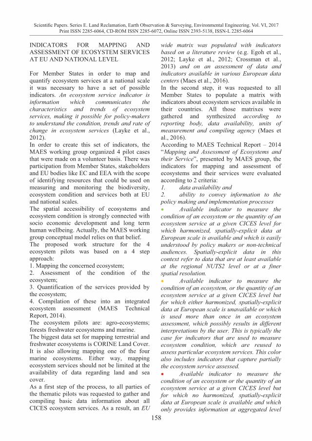
158
Scientific Papers. Series E. Land Reclamation, Earth Observation & Surveying, Environmental Engineering. Vol. VI, 2017Print ISSN 2285-6064, CD-ROM ISSN 2285-6072, Online ISSN 2393-5138, ISSN-L 2285-6064
INDICATORS FOR MAPPING AND ASSESSMENT OF ECOSYSTEM SERVICES AT EU AND NATIONAL LEVEL For Member States in order to map and quantify ecosystem services at a national scale it was necessary to have a set of possible indicators. An ecosystem service indicator is information which communicates the characteristics and trends of ecosystem services, making it possible for policy-makers to understand the condition, trends and rate of change in ecosystem services (Layke et al., 2012). In order to create this set of indicators, the MAES working group organized 4 pilot cases that were made on a volunteer basis. There was participation from Member States, stakeholders and EU bodies like EC and EEA with the scope of identifying resources that could be used on measuring and monitoring the biodiversity, ecosystem condition and services both at EU and national scales. The spatial accessibility of ecosystems and ecosystem condition is strongly connected with socio economic development and long term human wellbeing. Actually, the MAES working group conceptual model relies on that belief. The proposed work structure for the 4 ecosystem pilots was based on a 4 step approach: 1. Mapping the concerned ecosystem; 2. Assessment of the condition of the ecosystem; 3. Quantification of the services provided by the ecosystem; 4. Compilation of these into an integrated ecosystem assessment (MAES Technical Report, 2014). The ecosystem pilots are: agro-ecosystems; forests freshwater ecosystems and marine. The biggest data set for mapping terrestrial and freshwater ecosystems is CORINE Land Cover. It is also allowing mapping one of the four marine ecosystems. Either way, mapping ecosystem services should not be limited at the availability of data regarding land and sea cover. As a first step of the process, to all parties of the thematic pilots was requested to gather and compiling basic data information about all CICES ecosystem services. As a result, an EU
wide matrix was populated with indicators based on a literature review (e.g. Egoh et al., 2012; Layke et al., 2012; Crossman et al., 2013) and on an assessment of data and indicators available in various European data centers (Maes et al., 2016). In the second step, it was requested to all Member States to populate a matrix with indicators about ecosystem services available in their countries. All those matrixes were gathered and synthesized according to reporting body, data availability, units of measurement and compiling agency (Maes et al., 2016). According to MAES Technical Report – 2014 “Mapping and Assessment of Ecosystems and their Service”, presented by MAES group, the indicators for mapping and assessment of ecosystems and their services were evaluated according to 2 criteria: 1. data availability and 2. ability to convey information to the policy making and implementation processes � Available indicator to measure the condition of an ecosystem or the quantity of an ecosystem service at a given CICES level for which harmonized, spatially-explicit data at European scale is available and which is easily understood by policy makers or non-technical audiences. Spatially-explicit data in this context refer to data that are at least available at the regional NUTS2 level or at a finer spatial resolution. � Available indicator to measure the condition of an ecosystem, or the quantity of an ecosystem service at a given CICES level but for which either harmonized, spatially-explicit data at European scale is unavailable or which is used more than once in an ecosystem assessment, which possibly results in different interpretations by the user. This is typically the case for indicators that are used to measure ecosystem condition, which are reused to assess particular ecosystem services. This color also includes indicators that capture partially the ecosystem service assessed. � Available indicator to measure the condition of an ecosystem or the quantity of an ecosystem service at a given CICES level but for which no harmonized, spatially-explicit data at European scale is available and which only provides information at aggregated level
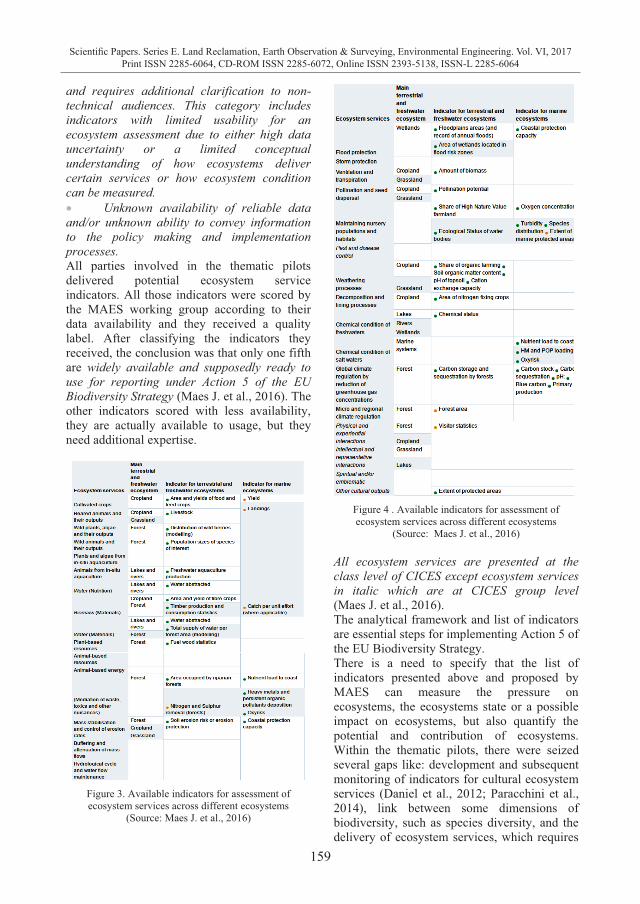
159
Scientific Papers. Series E. Land Reclamation, Earth Observation & Surveying, Environmental Engineering. Vol. VI, 2017Print ISSN 2285-6064, CD-ROM ISSN 2285-6072, Online ISSN 2393-5138, ISSN-L 2285-6064
and requires additional clarification to non-technical audiences. This category includes indicators with limited usability for an ecosystem assessment due to either high data uncertainty or a limited conceptual understanding of how ecosystems deliver certain services or how ecosystem condition can be measured. � Unknown availability of reliable data and/or unknown ability to convey information to the policy making and implementation processes. All parties involved in the thematic pilots delivered potential ecosystem service indicators. All those indicators were scored by the MAES working group according to their data availability and they received a quality label. After classifying the indicators they received, the conclusion was that only one fifth are widely available and supposedly ready to use for reporting under Action 5 of the EU Biodiversity Strategy (Maes J. et al., 2016). The other indicators scored with less availability, they are actually available to usage, but they need additional expertise.
Figure 3. Available indicators for assessment of ecosystem services across different ecosystems
(Source: Maes J. et al., 2016)
Figure 4 . Available indicators for assessment of ecosystem services across different ecosystems
(Source: Maes J. et al., 2016) All ecosystem services are presented at the class level of CICES except ecosystem services in italic which are at CICES group level (Maes J. et al., 2016). The analytical framework and list of indicators are essential steps for implementing Action 5 of the EU Biodiversity Strategy. There is a need to specify that the list of indicators presented above and proposed by MAES can measure the pressure on ecosystems, the ecosystems state or a possible impact on ecosystems, but also quantify the potential and contribution of ecosystems. Within the thematic pilots, there were seized several gaps like: development and subsequent monitoring of indicators for cultural ecosystem services (Daniel et al., 2012; Paracchini et al., 2014), link between some dimensions of biodiversity, such as species diversity, and the delivery of ecosystem services, which requires
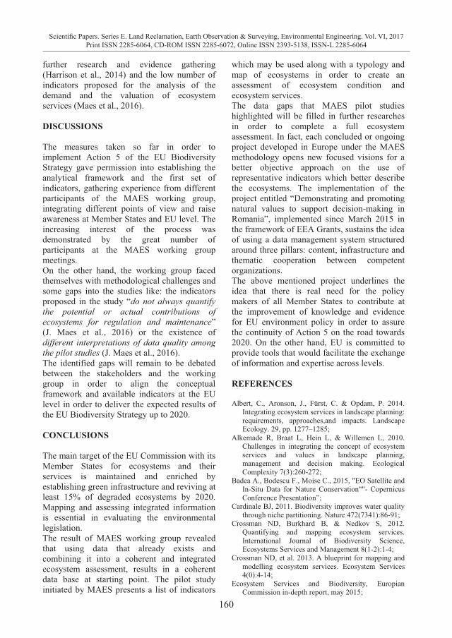
160
Scientific Papers. Series E. Land Reclamation, Earth Observation & Surveying, Environmental Engineering. Vol. VI, 2017Print ISSN 2285-6064, CD-ROM ISSN 2285-6072, Online ISSN 2393-5138, ISSN-L 2285-6064
further research and evidence gathering (Harrison et al., 2014) and the low number of indicators proposed for the analysis of the demand and the valuation of ecosystem services (Maes et al., 2016). DISCUSSIONS The measures taken so far in order to implement Action 5 of the EU Biodiversity Strategy gave permission into establishing the analytical framework and the first set of indicators, gathering experience from different participants of the MAES working group, integrating different points of view and raise awareness at Member States and EU level. The increasing interest of the process was demonstrated by the great number of participants at the MAES working group meetings. On the other hand, the working group faced themselves with methodological challenges and some gaps into the studies like: the indicators proposed in the study “do not always quantify the potential or actual contributions of ecosystems for regulation and maintenance” (J. Maes et al., 2016) or the existence of different interpretations of data quality among the pilot studies (J. Maes et al., 2016). The identified gaps will remain to be debated between the stakeholders and the working group in order to align the conceptual framework and available indicators at the EU level in order to deliver the expected results of the EU Biodiversity Strategy up to 2020. CONCLUSIONS The main target of the EU Commission with its Member States for ecosystems and their services is maintained and enriched by establishing green infrastructure and reviving at least 15% of degraded ecosystems by 2020. Mapping and assessing integrated information is essential in evaluating the environmental legislation. The result of MAES working group revealed that using data that already exists and combining it into a coherent and integrated ecosystem assessment, results in a coherent data base at starting point. The pilot study initiated by MAES presents a list of indicators
which may be used along with a typology and map of ecosystems in order to create an assessment of ecosystem condition and ecosystem services. The data gaps that MAES pilot studies highlighted will be filled in further researches in order to complete a full ecosystem assessment. In fact, each concluded or ongoing project developed in Europe under the MAES methodology opens new focused visions for a better objective approach on the use of representative indicators which better describe the ecosystems. The implementation of the project entitled “Demonstrating and promoting natural values to support decision-making in Romania”, implemented since March 2015 in the framework of EEA Grants, sustains the idea of using a data management system structured around three pillars: content, infrastructure and thematic cooperation between competent organizations. The above mentioned project underlines the idea that there is real need for the policy makers of all Member States to contribute at the improvement of knowledge and evidence for EU environment policy in order to assure the continuity of Action 5 on the road towards 2020. On the other hand, EU is committed to provide tools that would facilitate the exchange of information and expertise across levels. REFERENCES Albert, C., Aronson, J., Fürst, C. & Opdam, P. 2014.
Integrating ecosystem services in landscape planning: requirements, approaches,and impacts. Landscape Ecology. 29, pp. 1277–1285;
Alkemade R, Braat L, Hein L, & Willemen L, 2010. Challenges in integrating the concept of ecosystem services and values in landscape planning, management and decision making. Ecological Complexity 7(3):260-272;
Badea A., Bodescu F., Moise C., 2015, "EO Satellite and In-Situ Data for Nature Conservation""- Copernicus Conference Presentation”;
Cardinale BJ, 2011. Biodiversity improves water quality through niche partitioning. Nature 472(7341):86-91;
Crossman ND, Burkhard B, & Nedkov S, 2012. Quantifying and mapping ecosystem services. International Journal of Biodiversity Science, Ecosystems Services and Management 8(1-2):1-4;
Crossman ND, et al. 2013. A blueprint for mapping and modelling ecosystem services. Ecosystem Services 4(0):4-14;
Ecosystem Services and Biodiversity, Europian Commission in-depth report, may 2015;
161
Scientific Papers. Series E. Land Reclamation, Earth Observation & Surveying, Environmental Engineering. Vol. VI, 2017Print ISSN 2285-6064, CD-ROM ISSN 2285-6072, Online ISSN 2393-5138, ISSN-L 2285-6064
European Commission, 2011. Our life insurance, our natural capital: an EU biodiversity strategy to 2020. COM (2011) 244. Brussels;
European Commission, 2012. Improving the delivery of benefits from EU environment measures: building confidence through better knowledge and responsiveness. COM (2012) 95. Brussels;
European Commission, 2015. Mapping and assessment of forest ecosystems and their services; Applications and guidance for decision making in the framework of MAES;
Foley,M..M..,Halpern,B.S.,Micheli,F.,Armsby,M.H.,Caldwell,M.R.,Crain,C.M., Prahler, E., Rohr,N., Sivas,D., Beck, M.W., Carr, M.H., Crowder, L.B.,Emmett, Duffy, J., Hacker, S.D.,McLeod, K.L., Palumbi, S.R.,Peterson, C.H., Regan,H.M., Ruckelshaus,M.H.,Sandifer,P.A., Steneck,R.S.,2010 Guidingecological principles for marine spatial planning. Marine Policy 34, 955–966;
Haines-Young R, Potschin M, & Kienast F, 2012. Indicators of ecosystem service potential at European scales;
Haines-Young RH & Potschin MP, 2010. The links between biodiversity, ecosystem services and human wellbeing. Ecosystem Ecology: a new synthesis, eds Raffaelli DG & Frid CLJ (Cambridge University Press), p 162;
Herbei Mihai Valentin, Sala Florin, 2015, Use Landsat image to evaluate vegetation stage in sunflower crops, AgroLife Scientific Journal - Volume 4, Number 1, 2015;
Joachim Maes, Camino Liquete, Anne Teller, Markus Erhard, Maria Luisa Paracchinia, José I. Barredoa, Bruna Grizzettia, Ana Cardosoa, Francesca Sommaa, Jan-Erik Petersenc, Andrus Meinerc, Eva Royo Gelabertc, Nihat Zalc, Peter Kristensenc, Annemarie Bastrup-Birkc, Katarzyna Bialac, Chiara Piroddia, 1, Benis Egoha, 2, Patrick Degeorgesd, Christel Fiorinad, Fernando Santos-Martíne, Vytautas Naruševičiusf, Jan Verboveng, Henrique M. Pereirah, Jan Bengtssoni, 2016, An indicator framework for assessing ecosystem services in support of the EU Biodiversity Strategy to 2020, Ecosystem Services, Volume 17, February 2016, Pages 14–23;
Mace GM, Norris K, & Fitter AH, 2012. Biodiversity and ecosystem services: a multilayered relationship. Trends in Ecology & Evolution 27(1):19-26;
Maes et al, 2012. Mapping ecosystem services for policy support and decision making in the European Union;
Maes J et al, 2014. Mapping and Assessment of Ecosystems and their Services: Indicators for ecosystem assessments under Action 5 of the EU Biodiversity Strategy to 2020, 2nd Report of the EU Commission, February 2014;
Maes J et al, 2016, Mapping and Assessment of Ecosystems and their Services, 3nd Report of the EU Commission, march 2016;
Maes J, et al., 2012. A spatial assessment of ecosystem services in Europe: methods, case studies and policy analysis - Phase 2. Synthesis. PEER report no 4. Ispra. Partnership for European Environmental Research;
Maes J, et al., 2012. Mapping ecosystem services for policy support and decision making in the European Union. Ecosystem Services 1(1):31-39;
Maes J, et al., 2013. Mapping and Assessment of Ecosystems and their Services. An analytical framework for ecosystem assessments under action 5 of the EU biodiversity strategy to 2020. Publications office of the European Union, Luxembourg;
Maes J, Paracchini MP, Zulian G, & Alkemade R, 2012. Synergies and trade-offs between ecosystem service supply, biodiversity and habitat conservation status in Europe. Biological Conservation 155:1-12;
Mapping and Assessment of Ecosystems and their Services, 1st Report of the EU Commission: An analytical framework for ecosystem assessments under Action 5 of the EU Biodiversity Strategy to 2020; April 2013;
Mark L. Carroll, Molly E. Brown, Akiko Elders, and Kiersten Johnson, Feasibility of Using Remotely Sensed Data to Aid in Long-term Monitoring of Biodiversity; NASA/TM–2014;
Martnez-Harms MJ & Balvanera P, 2012. Methods for mapping ecosystem service supply: A review International Journal of Biodiversity Science, Ecosystems Services and Management 8(1-2):17-25;
Millennium Ecosystem Assessment, 2005. Ecosystems and human well-being: biodiversity synthesis. World Resources Institute. Washington, D.C. (USA);
Nedkov, S.,Burkhard,B., Flood regulating ecosystem services-Mapping supply and demand, in the Etropole municipality, Bulgaria. Ecological Indicators, in press;
Nelson, E.J.,Daily,G.C.,2010.Modeling ecosystem services in terrestrial systems. F1000 BiologyReports2:53http://dx.doi.org/10.3410/B2-53;
P.A. Harrison, M. Termansen, M. García-Llorente, P.M. Berry, Y.K. Bredin, M. Bucur, G. Cosor, D. García del Amo, N. Geamănă, E. Gomez Baggethun, L. Gónzalez, J.R. Haslett, I. Iniesta-Arandia, S. Li, H. Lindhjem, J.D. Linnell, B. Martín-Lopez, L. Mathieu, I. Palomo, A.C. Smith, R. Tinch and A. Vadineanu;2014. Final report on relationships between biodiversity, ecosystem services and values in case studies;
Pereira HM, Domingos T, & Vicente L, 2006. Assessing ecosystem services at different scales in the Portugal Millennium Ecosystem Assessment. Bridging Scales and Knowledge Systems, eds Reid W, Berks F, Wilbanks T,& Capistrano D (Island Press, Washington DC), pp 59-80;
Plummer, M.L.,2009.Assessing benefi ttransfer for the valuation ofe cosystem services. Frontiers in Ecology and the Environment7, 38–45;
Raudsepp-Hearne C, et al., 2005. Assessment Process. Ecosystems and Human Well-Being: Multi-Scales Assessments, eds Capistrano D & Samper C (Island Press, Washington DC), pp 119-140;
Secretariat of the Convention on Biological Diversity, 2010.Global Biodiversity Outlook 3.Montre´ al.
Tronac Augustina, Nistor Elena, Sarbu Nicoleta, 2013, Urban green space - environment and culture, AgroLife Scientific Journal - Volume 2, Number 2, 2013;

162
Scientific Papers. Series E. Land Reclamation, Earth Observation & Surveying, Environmental Engineering. Vol. VI, 2017Print ISSN 2285-6064, CD-ROM ISSN 2285-6072, Online ISSN 2393-5138, ISSN-L 2285-6064
Willemen, L., Veldkamp,A., Verburg,P.H., Hein,L., Leemans,R. ,2012. Amulti-scale modeling approach for analyzing landscape service dynamics. Journal of Environmental Management100,86–95;
Wouter Van Reeth, Heikki Toivonen, Frédéric Gosselin, Jacques Baudry, Leon Braat, Karl Baadsvik, John Linnell, Angheluta Vadineanu, Jana Sedláková & Irene Bouwma;2005. A Long-Term Biodiversity, Ecosystem and Awareness Research Network; European Commission’s Sixth Framework Programme for Research and Development;
http://biodiversity.europa.eu/maes; http://ec.europa.eu/environment/integration/research/new
salert/index_en.htm;
http://ec.europa.eu/environment/nature/knowledge/ecosystem_assessment/index_en.htm;
http://ec.europa.eu/environment/nature/knowledge/ecosystem_assessment/pdf/2ndMAESWorkingPaper.pdf;
http://ec.europa.eu/environment/nature/knowledge/ecosystem_assessment/pdf/MAESWorkingPaper2013.pdf
http://www.eisceuropa.eu/images/stories/2016q1/2016EISC_Workshop_Presentations/02_Badea.pdf;
http://biodiversity.europa.eu/maes/mapping-ecosystems/indicators-for-ecosystem-services-across-ecosystems;
http://biodiversity.europa.eu/maes/mapping-ecosystems/indicators-of-ecosystem-condition
163
Scientific Papers. Series E. Land Reclamation, Earth Observation & Surveying, Environmental Engineering. Vol. VI, 2017Print ISSN 2285-6064, CD-ROM ISSN 2285-6072, Online ISSN 2393-5138, ISSN-L 2285-6064
Willemen, L., Veldkamp,A., Verburg,P.H., Hein,L., Leemans,R. ,2012. Amulti-scale modeling approach for analyzing landscape service dynamics. Journal of Environmental Management100,86–95;
Wouter Van Reeth, Heikki Toivonen, Frédéric Gosselin, Jacques Baudry, Leon Braat, Karl Baadsvik, John Linnell, Angheluta Vadineanu, Jana Sedláková & Irene Bouwma;2005. A Long-Term Biodiversity, Ecosystem and Awareness Research Network; European Commission’s Sixth Framework Programme for Research and Development;
http://biodiversity.europa.eu/maes; http://ec.europa.eu/environment/integration/research/new
salert/index_en.htm;
http://ec.europa.eu/environment/nature/knowledge/ecosystem_assessment/index_en.htm;
http://ec.europa.eu/environment/nature/knowledge/ecosystem_assessment/pdf/2ndMAESWorkingPaper.pdf;
http://ec.europa.eu/environment/nature/knowledge/ecosystem_assessment/pdf/MAESWorkingPaper2013.pdf
http://www.eisceuropa.eu/images/stories/2016q1/2016EISC_Workshop_Presentations/02_Badea.pdf;
http://biodiversity.europa.eu/maes/mapping-ecosystems/indicators-for-ecosystem-services-across-ecosystems;
http://biodiversity.europa.eu/maes/mapping-ecosystems/indicators-of-ecosystem-condition
REMOTE SENSING FOR DESERTIFICATION MONITORING
IN BRAILA COUNTY
Catalina BORDUN (FLOREA-GABRIAN), Sorin Mihai CIMPEANU
University of Agronomic Sciences and Veterinary Medicine of Bucharest,
59 Marasti Blvd, District 1, Bucharest, Romania
Corresponding author email: [email protected]
Abstract Desertification of agricultural areas has been growing as a key subject in continental land management, as large parts of traditional farming zones degraded over the years, as a consequence of climate changes and antropic vicious actions. Soil degradation up to desertification of large agricultural areas in Braila county plains, results as an interaction between local salinised soil and climate variation, leading to long periods of draoughts. Remote sensing for the determination of the intensity and extension of desertified areas is a solution to better understand the impact of this phenomena in Braila county. The objective of this paper is to determine whether climatic variations continue the present trend, through a comparation based on the Normalized Difference Drought Index – NDDI from MODIS producs processed with spatial analyst of ArcGis, for 2000-2005-2010-2016. The time interval was chosen due to agroclimatheric classifications, considering 2000 is classified as draght year, 20005 a normal climateric year and 2010 a rainy year. A multi-temporal series of MODIS data were gathered, 8 days synthesis, in order to determine NDDI, with empirical formulas based on the spatial images computed values, for the normalised differenced vegetation index – NDVI and normalised difference water index – NDWI. Measuring the NDVI variation based on the clorofile absorbed radiation in the red spectral band and closed infrared reflectancy, allowed us to identify the impact on vegetation cover, while computing NDWI from green and closed infrared spectral band, delivered information on the vegetation water content. The resulted values of NDDI, computed for the vegetation period, April to October, confirm 2016 as a rather normal year for agricultural purpose.
Key words: agriculture, desertification, land degradation, remote sensing
INTRODUCTION Agricultural soil quality has been an important issue forever, both for the intensive and extensive growing systems. Engineering solutions to upgrade the soil production capacity are being developed continuously, but applied over long periods of time, resulted in depraved ecosystems consequences. It is the case of parts of Braila County in Romania, where large traditional agricultural areas converted to deserted zones, as a result of natural local conditions, land reclamation systems and climatic conditions. Since 1997, Romania has ratified the UNCCD convention, through Law 629 and National Strategies and Action Plans have been elaborated in order to identify problem areas and solutions to control and combat desertification and its catastrophic conse-quences. Soil and ecosystems quality eva-luation for the studied area have been conducted since 1970’s, along with the
development and implementation of the land reclamation systems. The main engineering works consisted in irrigation and drainage structures, aiming to protect agricultural crops against natural drought and high levels of phreatic waters, Braila County being the second county with more than 380,000 km2 of agricultural areas with land reclamation works in the country, after Constanta County. The studied area is situated in south – east of Romania and is part of the Romanian Plain, one of the most productive agricultural zones in the country. Intensification and extension of the soil degradation processes along with higher natural environmental resources vulnerability to aggressive factors, is a consequence of the agricultural industrialisation and technology severe rhythm, in order to multiply the productivity and contribution of agriculture to the economic development of the country (Robescu, 2008).
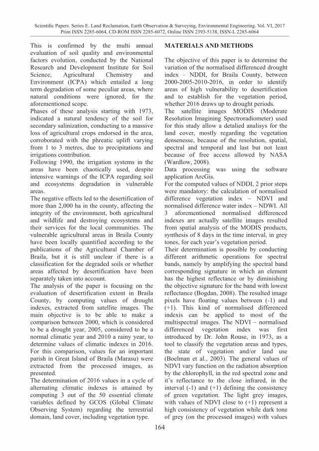
164
Scientific Papers. Series E. Land Reclamation, Earth Observation & Surveying, Environmental Engineering. Vol. VI, 2017Print ISSN 2285-6064, CD-ROM ISSN 2285-6072, Online ISSN 2393-5138, ISSN-L 2285-6064
This is confirmed by the multi annual evaluation of soil quality and environmental factors evolution, conducted by the National Research and Development Institute for Soil Science, Agricultural Chemistry and Environment (ICPA) which entailed a long term degradation of some peculiar areas, where natural conditions were ignored, for the aforementioned scope. Phases of these analysis starting with 1973, indicated a natural tendency of the soil for secondary salinization, conducting to a massive loss of agricultural crops endorsed in the area, corroborated with the phreatic uplift varying from 1 to 3 metres, due to precipitations and irrigations contribution. Following 1990, the irrigation systems in the areas have been chaotically used, despite intensive warnings of the ICPA regarding soil and ecosystems degradation in vulnerable areas. The negative effects led to the desertification of more than 2,000 ha in the county, affecting the integrity of the environment, both agricultural and wildlife and destroying ecosystems and their services for the local communities. The vulnerable agricultural areas in Braila County have been locally quantified according to the publications of the Agricultural Chamber of Braila, but it is still unclear if there is a classification for the degraded soils or whether areas affected by desertification have been separately taken into account. The analysis of the paper is focusing on the evaluation of desertification extent in Braila County, by computing values of drought indexes, extracted from satellite images. The main objective is to be able to make a comparison between 2000, which is considered to be a drought year, 2005, considered to be a normal climatic year and 2010 a rainy year, to determine values of climatic indexes in 2016. For this comparison, values for an important parish in Great Island of Braila (Marasu) were extracted from the processed images, as presented. The determination of 2016 values in a cycle of alternating climatic indexes is attained by computing 3 out of the 50 essential climate variables defined by GCOS (Global Climate Observing System) regarding the terrestrial domain, land cover, including vegetation type.
MATERIALS AND METHODS The objective of this paper is to determine the variation of the normalised differenced drought index – NDDI, for Braila County, between 2000-2005-2010-2016, in order to identify areas of high vulnerability to desertification and to establish for the vegetation period, whether 2016 draws up to drought periods. The satellite images MODIS (Moderate Resolution Imagining Spectroradiometer) used for this study allow a detalied analisys for the land cover, mostly regarding the vegetation densenesse, because of the resolution, spatial, spectral and temporal and last but not least because of free access allowed by NASA (Wardlow, 2008). Data processing was using the software application ArcGis. For the computed values of NDDI, 2 prior steps were mandatory: the calculation of normalised difference vegetation index – NDVI and normalised difference water index – NDWI. All 3 aforementioned normalised differenced indexes are actually satellite images resulted from spatial analysis of the MODIS products, synthesis of 8 days in the time interval, in grey tones, for each year’s vegetation period. Their determination is possible by conducting different arithmetic operations for spectral bands, namely by amplifying the spectral band corresponding signature in which an element has the highest reflectance or by diminishing the objective signature for the band with lowest reflectance (Bogdan, 2008). The resulted image pixels have floating values between (-1) and (+1). This kind of normalised differenced indexis can be applied to most of the multispectral images. The NDVI – normalised differenced vegetation index was first introduced by Dr. John Rouse, in 1973, as a tool to classify the vegetation areas and types, the state of vegetation and/or land use (Boelman et al., 2003). The general values of NDVI vary function on the radiation absorption by the chlorophyll, in the red spectral zone and it’s reflectance to the close infrared, in the interval (-1) and (+1) defining the consistency of green vegetation. The light grey images, with values of NDVI close to (+1) represent a high consistency of vegetation while dark tone of grey (on the processed images) with values
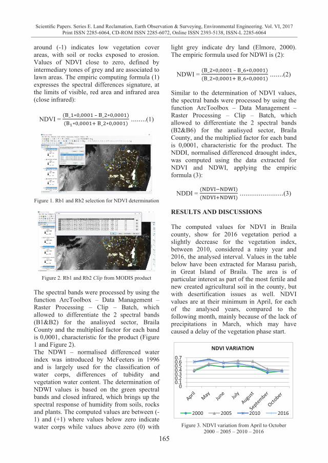
165
Scientific Papers. Series E. Land Reclamation, Earth Observation & Surveying, Environmental Engineering. Vol. VI, 2017Print ISSN 2285-6064, CD-ROM ISSN 2285-6072, Online ISSN 2393-5138, ISSN-L 2285-6064
around (-1) indicates low vegetation cover areas, with soil or rocks exposed to erosion. Values of NDVI close to zero, defined by intermediary tones of grey and are associated to lawn areas. The empiric computing formula (1) expresses the spectral differences signature, at the limits of visible, red area and infrared area (close infrared):
NDVI = ........(1)
Figure 1. Rb1 and Rb2 selection for NDVI determination
Figure 2. Rb1 and Rb2 Clip from MODIS product
The spectral bands were processed by using the function ArcToolbox – Data Management – Raster Processing – Clip – Batch, which allowed to differentiate the 2 spectral bands (B1&B2) for the analisyed sector, Braila County and the multiplied factor for each band is 0,0001, characteristic for the product (Figure 1 and Figure 2). The NDWI – normalised differenced water index was introduced by McFeeters in 1996 and is largely used for the classification of water corps, differences of tubidity and vegetation water content. The determination of NDWI values is based on the green spectral bands and closed infrared, which brings up the spectral response of humidity from soils, rocks and plants. The computed values are between (-1) and (+1) where values below zero indicate water corps while values above zero (0) with
light grey indicate dry land (Elmore, 2000). The empiric formula used for NDWI is (2):
NDWI = .......(2)
Similar to the determination of NDVI values, the spectral bands were processed by using the function ArcToolbox – Data Management – Raster Processing – Clip – Batch, which allowed to differentiate the 2 spectral bands (B2&B6) for the analisyed sector, Braila County, and the multiplied factor for each band is 0,0001, characteristic for the product. The NDDI, normalised differenced draought index, was computed using the data extracted for NDVI and NDWI, applying the empiric formula (3):
NDDI = .......................(3)
RESULTS AND DISCUSSIONS The computed values for NDVI in Braila county, show for 2016 vegetation period a slightly decrease for the vegetation index, between 2010, considered a rainy year and 2016, the analysed interval. Values in the table below have been extracted for Marasu parish, in Great Island of Braila. The area is of particular interest as part of the most fertile and new created agricultural soil in the county, but with desertification issues as well. NDVI values are at their minimum in April, for each of the analysed years, compared to the following month, mainly because of the lack of precipitations in March, which may have caused a delay of the vegetation phase start.
Figure 3. NDVI variation from April to October
2000 – 2005 – 2010 – 2016
00.10.20.30.40.50.60.7
2000 2005 2010 2016
NDVI VARIATION
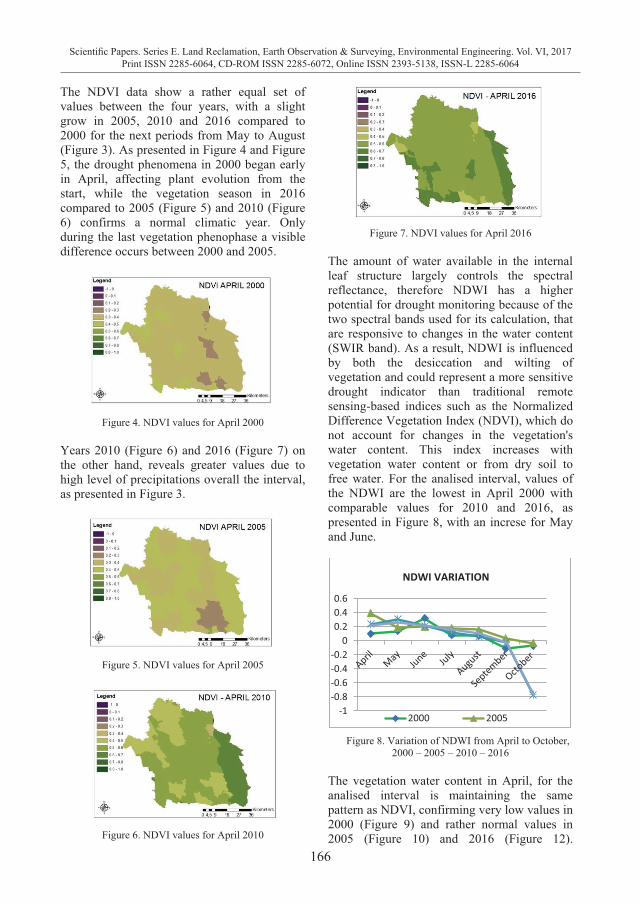
166
Scientific Papers. Series E. Land Reclamation, Earth Observation & Surveying, Environmental Engineering. Vol. VI, 2017Print ISSN 2285-6064, CD-ROM ISSN 2285-6072, Online ISSN 2393-5138, ISSN-L 2285-6064
The NDVI data show a rather equal set of values between the four years, with a slight grow in 2005, 2010 and 2016 compared to 2000 for the next periods from May to August (Figure 3). As presented in Figure 4 and Figure 5, the drought phenomena in 2000 began early in April, affecting plant evolution from the start, while the vegetation season in 2016 compared to 2005 (Figure 5) and 2010 (Figure 6) confirms a normal climatic year. Only during the last vegetation phenophase a visible difference occurs between 2000 and 2005.
Figure 4. NDVI values for April 2000
Years 2010 (Figure 6) and 2016 (Figure 7) on the other hand, reveals greater values due to high level of precipitations overall the interval, as presented in Figure 3.
Figure 5. NDVI values for April 2005
Figure 6. NDVI values for April 2010
Figure 7. NDVI values for April 2016
The amount of water available in the internal leaf structure largely controls the spectral reflectance, therefore NDWI has a higher potential for drought monitoring because of the two spectral bands used for its calculation, that are responsive to changes in the water content (SWIR band). As a result, NDWI is influenced by both the desiccation and wilting of vegetation and could represent a more sensitive drought indicator than traditional remote sensing-based indices such as the Normalized Difference Vegetation Index (NDVI), which do not account for changes in the vegetation's water content. This index increases with vegetation water content or from dry soil to free water. For the analised interval, values of the NDWI are the lowest in April 2000 with comparable values for 2010 and 2016, as presented in Figure 8, with an increse for May and June.
Figure 8. Variation of NDWI from April to October,
2000 – 2005 – 2010 – 2016
The vegetation water content in April, for the analised interval is maintaining the same pattern as NDVI, confirming very low values in 2000 (Figure 9) and rather normal values in 2005 (Figure 10) and 2016 (Figure 12).
-1-0.8-0.6-0.4-0.2
00.20.40.6
2000 2005
NDWI VARIATION
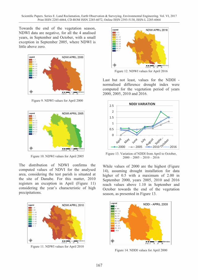
167
Scientific Papers. Series E. Land Reclamation, Earth Observation & Surveying, Environmental Engineering. Vol. VI, 2017Print ISSN 2285-6064, CD-ROM ISSN 2285-6072, Online ISSN 2393-5138, ISSN-L 2285-6064
Towards the end of the vegetation season, NDWI data are negative, for all the 4 analised years, in September and October, with a small exception in September 2005, where NDWI is little above zero.
Figure 9. NDWI values for April 2000
Figure 10. NDWI values for April 2005
The distribution of NDWI confirms the computed values of NDVI for the analysed area, considering the test parish is situated at the site of Danube. For this matter, 2010 registers an exception in April (Figure 11) considering the year’s characteristic of high precipitations.
Figure 11. NDWI values for April 2010
Figure 12. NDWI values for April 2016 Last but not least, values for the NDDI - normalised difference drought index were computed for the vegetation period of years 2000, 2005, 2010 and 2016.
Figure 13. Variation of NDDI from April to October,
2000 – 2005 – 2010 – 2016
While values of 2000 are the highest (Figure 14), assuming drought installation for data higher of 0.5 with a maximum of 2.00 in September 2000, years 2005, 2010 and 2016 reach values above 1.10 in September and October towards the end of the vegetation season, as presented in Figure 13.
Figure 14. NDDI values for April 2000
0
0.5
1
1.5
2
2.5
2000 2005 2010 2016
NDDI VARIATION
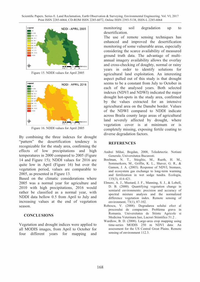
168
Scientific Papers. Series E. Land Reclamation, Earth Observation & Surveying, Environmental Engineering. Vol. VI, 2017Print ISSN 2285-6064, CD-ROM ISSN 2285-6072, Online ISSN 2393-5138, ISSN-L 2285-6064
Figure 15. NDDI values for April 2005
Figure 16. NDDI values for April 2005
By combining the three indexes for drought “pattern” the desertification tendency is recognizable for the study area, confirming the effects of low precipitations and high temperatures in 2000 compared to 2005 (Figure 14 and Figure 15); NDDI values for 2016 are quite low in April (Figure 16) but over the vegetation period, values are comparable to 2005, as presented in Figure 13. Based on the climatic considerations where 2005 was a normal year for agriculture and 2010 with high precipitations, 2016 would rather be classified as a normal year, with NDDI data bellow 0.5 from April to July and increasing values at the end of vegetation season.
CONCLUSIONS
Vegetation and drought indices were applied to all MODIS images, from April to October for four different years for mapping and
monitoring soil degradation up to desertification. The use of remote sensing techniques has enhanced and improved the desertification monitoring of some vulnerable areas, especially considering the scarce availability of measured ground truth data. The advantage of multi-annual imagery availability allows the overlay and cross-checking of doughty, normal or rainy years in order to identify solutions for agricultural land exploitation. An interesting aspect pulled out of this study is that drought seems to be a constant from July to October in each of the analysed years. Both selected indexes (NDVI and NDWI) indicated the major drought hot-spots in the study area, confirmed by the values extracted for an intensive agricultural area on the Danube border. Values of the NDWI compared to NDDI indicate across Braila county large areas of agricultural land severely affected by drought, where vegetation cover is at minimum or is completely missing, exposing fertile coating to diverse degradation factors.
REFERENCES
Andrei Mihai, Bogdan, 2008, Teledetectie. Notiuni Generale, Universitatea Bucuresti.
Boelman, N. T., Stieglitz, M., Rueth, H. M., Sommerkorn, M., Griffin, K. L., Shaver, G. R., & Gamon, J. A. (2003). Response of NDVI, biomass, and ecosystem gas exchange to long-term warming and fertilization in wet sedge tundra. Ecologia, 135(3), 414-421.
Elmore, A. J., Mustard, J. F., Manning, S. J., & Lobell, D. B. (2000). Quantifying vegetation change in semiarid environments: precision and accuracy of spectral mixture analysis and the normalized difference vegetation index. Remote sensing of environment, 73(1), 87-102.
Robescu, V. (2008). Degradarea solului efect al procesului de compactare. Problema grava in Romania. Universitatea de Stiinte Agricole si Medicina Veterinara Iasi, Lucrsri Stiintifice 51.2 .
Wardlow, B. D. (2008). Large-area crop mapping using time-series MODIS 250 m NDVI data: An assessment for the US Central Great Plains. Remote sensing of environment 112.3.
169
Scientific Papers. Series E. Land Reclamation, Earth Observation & Surveying, Environmental Engineering. Vol. VI, 2017Print ISSN 2285-6064, CD-ROM ISSN 2285-6072, Online ISSN 2393-5138, ISSN-L 2285-6064
Figure 15. NDDI values for April 2005
Figure 16. NDDI values for April 2005
By combining the three indexes for drought “pattern” the desertification tendency is recognizable for the study area, confirming the effects of low precipitations and high temperatures in 2000 compared to 2005 (Figure 14 and Figure 15); NDDI values for 2016 are quite low in April (Figure 16) but over the vegetation period, values are comparable to 2005, as presented in Figure 13. Based on the climatic considerations where 2005 was a normal year for agriculture and 2010 with high precipitations, 2016 would rather be classified as a normal year, with NDDI data bellow 0.5 from April to July and increasing values at the end of vegetation season.
CONCLUSIONS
Vegetation and drought indices were applied to all MODIS images, from April to October for four different years for mapping and
monitoring soil degradation up to desertification. The use of remote sensing techniques has enhanced and improved the desertification monitoring of some vulnerable areas, especially considering the scarce availability of measured ground truth data. The advantage of multi-annual imagery availability allows the overlay and cross-checking of doughty, normal or rainy years in order to identify solutions for agricultural land exploitation. An interesting aspect pulled out of this study is that drought seems to be a constant from July to October in each of the analysed years. Both selected indexes (NDVI and NDWI) indicated the major drought hot-spots in the study area, confirmed by the values extracted for an intensive agricultural area on the Danube border. Values of the NDWI compared to NDDI indicate across Braila county large areas of agricultural land severely affected by drought, where vegetation cover is at minimum or is completely missing, exposing fertile coating to diverse degradation factors.
REFERENCES
Andrei Mihai, Bogdan, 2008, Teledetectie. Notiuni Generale, Universitatea Bucuresti.
Boelman, N. T., Stieglitz, M., Rueth, H. M., Sommerkorn, M., Griffin, K. L., Shaver, G. R., & Gamon, J. A. (2003). Response of NDVI, biomass, and ecosystem gas exchange to long-term warming and fertilization in wet sedge tundra. Ecologia, 135(3), 414-421.
Elmore, A. J., Mustard, J. F., Manning, S. J., & Lobell, D. B. (2000). Quantifying vegetation change in semiarid environments: precision and accuracy of spectral mixture analysis and the normalized difference vegetation index. Remote sensing of environment, 73(1), 87-102.
Robescu, V. (2008). Degradarea solului efect al procesului de compactare. Problema grava in Romania. Universitatea de Stiinte Agricole si Medicina Veterinara Iasi, Lucrsri Stiintifice 51.2 .
Wardlow, B. D. (2008). Large-area crop mapping using time-series MODIS 250 m NDVI data: An assessment for the US Central Great Plains. Remote sensing of environment 112.3.
GIS TECHNOLOGY USED FOR FLOODS STUDY
Zoltán FERENCZ, Aurelian Stelian HILA, Sorin Mihai CIMPEANU
University of Agronomic Sciences and Veterinary Medicine of Bucharest, 59 Marasti Blvd,
District 1, Bucharest, Romania
Corresponding author email: [email protected]
Abstract The objective of the study is to develop a Geographic Information System (GIS) model which integrates a lot of information and various types of data required for hydrographic and geomorphologic analyses, applicable in the sphere of hydrology and geomorphology. The case study will show how to use a GIS tool, create a Digital Elevation Model (DEM), using terrain information, contours line with height information attached and rivers, and at the end to obtain watershed boundaries and determine which basins have higher possibility of flooding by analysis of its shape. The raw data (primary database) will be obtained through vectorization from different maps used for analysing the geographic characteristics of the studied area. The paper focuses on prevention of potential disasters (floods), providing support in data collection and processing by transposing the real geographical problems in a computer-assisted modelling. Key words: DEM, geomorphology, hydrology, GIS. INTRODUCTION The aim of the study is to implement GIS technology in landscape modelling (studying the topographical surface) by numerical methods, having application in hydrology and geomorphology. The fundamental objective of this study is to prevent any disasters and predict in a very clear manner which are the areas with the highest potential risk in the case of floods, focusing on achieving a geographic informational system which integrates all kind of information, all types of data that are needed for hydrological analyses from the automatic extraction of the river basins, watersheds, as well as finding those that have the highest risk of flooding, till study the gradients and orientations of the slopes. Using GIS there is the possibility to conduct analyses and correlation of great complexity, which cannot be achieved with classical techniques (Balteanu et al., 2010), having in mind that the action of the natural factors is dependent on the local conditions (Lungu et al., 2015). Basically floods have a strong impact on environment as well as on local economies (Stepanova and Rubel, 2015) and the reason which supports the use of GIS techniques in
hydrology are that it’s lead to achieve the goal in a definitely better manner, being no other practical methods of achieving those objectives. MATERIALS AND METHODS The softwares used for the study is the ArcGIS package, more accurate the ArcMap 10.1 program with extensions and ArcScene 10.1. To obtain the Digital Elevation Model (DEM), we vectorized a topographic map (which was spatially referenced, Stereographic 1970 projection) at scale 1: 25000 with the increments between contour lines of 10 meters and for the remainder graphic database (rivers, creeks, lake, countrysides), we used topographic maps at scale 1:5000 and orthophotomap up to date. Primary database it was established by the followings layers (organized multilevel), which is presented in Table 1. The first step in the implementation of the database it was represented by procuring cartographic materials, while the second step it was to convert the information from the analogic raster support to vector format through vectorial entities as points, lines and polygons.
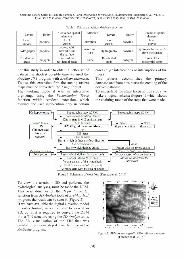
170
Scientific Papers. Series E. Land Reclamation, Earth Observation & Surveying, Environmental Engineering. Vol. VI, 2017Print ISSN 2285-6064, CD-ROM ISSN 2285-6072, Online ISSN 2393-5138, ISSN-L 2285-6064
Table 1. Primary graphical database structure
Layers Entity Contained spatial elements
Attributes Layers Entity Contained spatial
elements Level curves polyline level
curves elevation Level curves polyline level
curves
Hydrography polyline hydrographic network from
the surface
name and type Hydrography polyline hydrographic network
from the surface
Residential areas polygon limits of the
residential areas name Residential areas polygon limits of the
residential areas For this study in order to obtain a better set of data in the shortest possible time we used the ArcMap 10.1 program with ArcScan extension. To use this extension first the analog rasters maps must be converted into *.bmp format. The working mode it was an interactive digitizing, using the Vectorization Trace function within ArcScan extension, which requires the user intervention only in certain
cases (e. g.: intersections or interruptions of the lines). This process accomplishes the primary database and from now starts the creating of the derived database. To understand the steps taken in this study we make a logical schema (Figure 1) which shows the chaining-mode of the steps that were made.
Figure 1. Schematic of workflow (Ferencz et al., 2016)
To view the terrain in 3D and performe the hydrological analyses, must be made the DEM. This was done using the Topo to Raster function from 3D Analyst tools of ArcMap 10.1 program, the result can be seen in (Figure 2). If we have available the digital elevation model in raster format, we can choose to view it in 3D, but first is required to convert the DEM into a TIN structure using the 3D Analyst tools. The 3D visualization of the TIN that was created in previous step it must be done in the ArcScene program.
Figure 2. DEM in Stereografic 1970 reference system
(Ferencz et al., 2016)
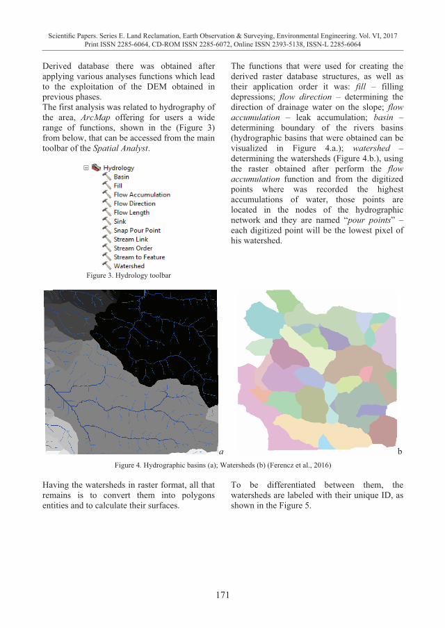
171
Scientific Papers. Series E. Land Reclamation, Earth Observation & Surveying, Environmental Engineering. Vol. VI, 2017Print ISSN 2285-6064, CD-ROM ISSN 2285-6072, Online ISSN 2393-5138, ISSN-L 2285-6064
Table 1. Primary graphical database structure
Layers Entity Contained spatial elements
Attributes Layers Entity Contained spatial
elements Level curves polyline level
curves elevation Level curves polyline level
curves
Hydrography polyline hydrographic network from
the surface
name and type Hydrography polyline hydrographic network
from the surface
Residential areas polygon limits of the
residential areas name Residential areas polygon limits of the
residential areas For this study in order to obtain a better set of data in the shortest possible time we used the ArcMap 10.1 program with ArcScan extension. To use this extension first the analog rasters maps must be converted into *.bmp format. The working mode it was an interactive digitizing, using the Vectorization Trace function within ArcScan extension, which requires the user intervention only in certain
cases (e. g.: intersections or interruptions of the lines). This process accomplishes the primary database and from now starts the creating of the derived database. To understand the steps taken in this study we make a logical schema (Figure 1) which shows the chaining-mode of the steps that were made.
Figure 1. Schematic of workflow (Ferencz et al., 2016)
To view the terrain in 3D and performe the hydrological analyses, must be made the DEM. This was done using the Topo to Raster function from 3D Analyst tools of ArcMap 10.1 program, the result can be seen in (Figure 2). If we have available the digital elevation model in raster format, we can choose to view it in 3D, but first is required to convert the DEM into a TIN structure using the 3D Analyst tools. The 3D visualization of the TIN that was created in previous step it must be done in the ArcScene program.
Figure 2. DEM in Stereografic 1970 reference system
(Ferencz et al., 2016)
Derived database there was obtained after applying various analyses functions which lead to the exploitation of the DEM obtained in previous phases. The first analysis was related to hydrography of the area, ArcMap offering for users a wide range of functions, shown in the (Figure 3) from below, that can be accessed from the main toolbar of the Spatial Analyst.
Figure 3. Hydrology toolbar
The functions that were used for creating the derived raster database structures, as well as their application order it was: fill – filling depressions; flow direction – determining the direction of drainage water on the slope; flow accumulation – leak accumulation; basin – determining boundary of the rivers basins (hydrographic basins that were obtained can be visualized in Figure 4.a.); watershed – determining the watersheds (Figure 4.b.), using the raster obtained after perform the flow accumulation function and from the digitized points where was recorded the highest accumulations of water, those points are located in the nodes of the hydrographic network and they are named “pour points” – each digitized point will be the lowest pixel of his watershed.
a b Figure 4. Hydrographic basins (a); Watersheds (b) (Ferencz et al., 2016)
Having the watersheds in raster format, all that remains is to convert them into polygons entities and to calculate their surfaces.
To be differentiated between them, the watersheds are labeled with their unique ID, as shown in the Figure 5.
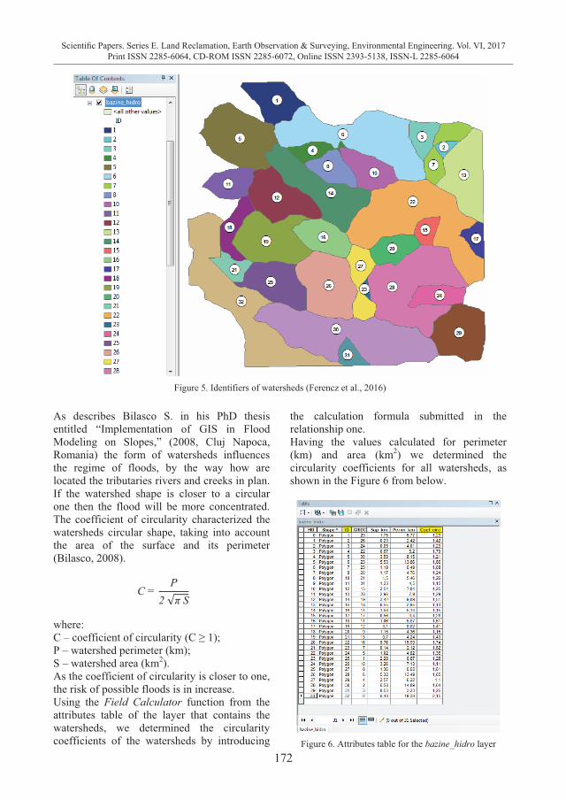
172
Scientific Papers. Series E. Land Reclamation, Earth Observation & Surveying, Environmental Engineering. Vol. VI, 2017Print ISSN 2285-6064, CD-ROM ISSN 2285-6072, Online ISSN 2393-5138, ISSN-L 2285-6064
Figure 5. Identifiers of watersheds (Ferencz et al., 2016)
As describes Bilasco S. in his PhD thesis entitled “Implementation of GIS in Flood Modeling on Slopes,” (2008, Cluj Napoca, Romania) the form of watersheds influences the regime of floods, by the way how are located the tributaries rivers and creeks in plan. If the watershed shape is closer to a circular one then the flood will be more concentrated. The coefficient of circularity characterized the watersheds circular shape, taking into account the area of the surface and its perimeter (Bilasco, 2008).
C = P
2 π S
where: C – coefficient of circularity (C ≥ 1); P – watershed perimeter (km); S – watershed area (km2). As the coefficient of circularity is closer to one, the risk of possible floods is in increase. Using the Field Calculator function from the attributes table of the layer that contains the watersheds, we determined the circularity coefficients of the watersheds by introducing
the calculation formula submitted in the relationship one. Having the values calculated for perimeter (km) and area (km2) we determined the circularity coefficients for all watersheds, as shown in the Figure 6 from below.
Figure 6. Attributes table for the bazine_hidro layer
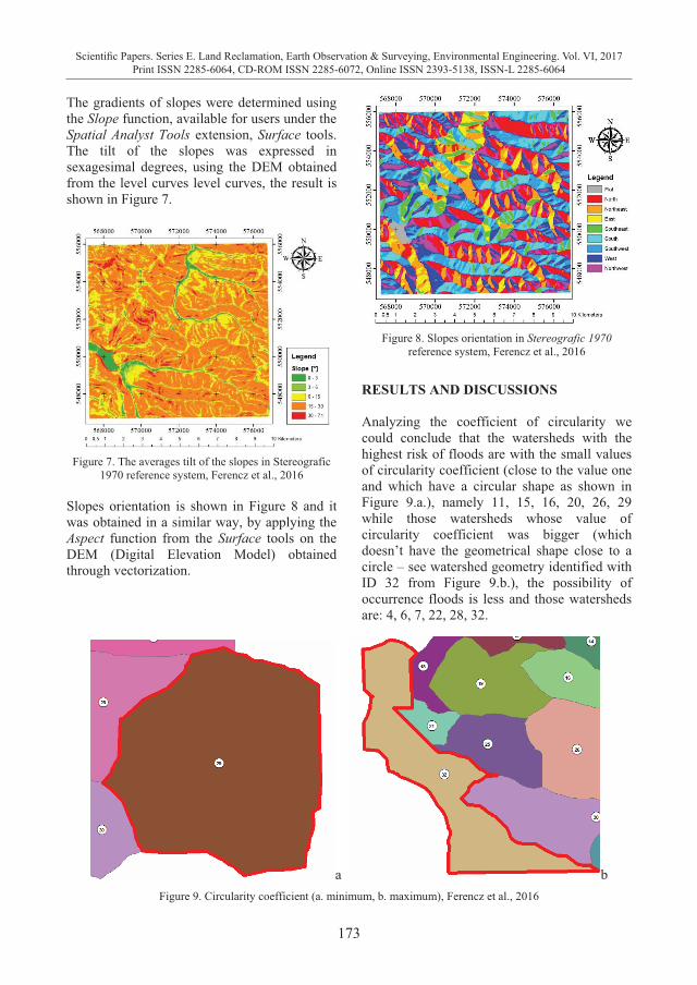
173
Scientific Papers. Series E. Land Reclamation, Earth Observation & Surveying, Environmental Engineering. Vol. VI, 2017Print ISSN 2285-6064, CD-ROM ISSN 2285-6072, Online ISSN 2393-5138, ISSN-L 2285-6064
The gradients of slopes were determined using the Slope function, available for users under the Spatial Analyst Tools extension, Surface tools. The tilt of the slopes was expressed in sexagesimal degrees, using the DEM obtained from the level curves level curves, the result is shown in Figure 7.
Figure 7. The averages tilt of the slopes in Stereografic
1970 reference system, Ferencz et al., 2016
Slopes orientation is shown in Figure 8 and it was obtained in a similar way, by applying the Aspect function from the Surface tools on the DEM (Digital Elevation Model) obtained through vectorization.
Figure 8. Slopes orientation in Stereografic 1970
reference system, Ferencz et al., 2016
RESULTS AND DISCUSSIONS Analyzing the coefficient of circularity we could conclude that the watersheds with the highest risk of floods are with the small values of circularity coefficient (close to the value one and which have a circular shape as shown in Figure 9.a.), namely 11, 15, 16, 20, 26, 29 while those watersheds whose value of circularity coefficient was bigger (which doesn’t have the geometrical shape close to a circle – see watershed geometry identified with ID 32 from Figure 9.b.), the possibility of occurrence floods is less and those watersheds are: 4, 6, 7, 22, 28, 32.
a b
Figure 9. Circularity coefficient (a. minimum, b. maximum), Ferencz et al., 2016
174
Scientific Papers. Series E. Land Reclamation, Earth Observation & Surveying, Environmental Engineering. Vol. VI, 2017Print ISSN 2285-6064, CD-ROM ISSN 2285-6072, Online ISSN 2393-5138, ISSN-L 2285-6064
The coefficient of circularity is the radius of the circle in which the watershed is inscribed. Radius is measured from the gravity center of the watershed. The map of slopes and the map of slopes orientations are part of the elevation data, which can be used to perform a variety of cartographic analyses (ESRI, 2012). Looking at the map of the slopes it can be observed that it is a predominantly mountainous area with an average inclination of slopes situated between the range of (150, 300), which was obvious on the topographic map also, given the short planimetric distance between the level curves lines. CONCLUSIONS This study presents theoretical and experimental information for the implementation of a geographic information system in order to provide standard products as maps and statistical tables used for risk calculation of the areas. After storing information inside of a GIS and applying on them several sets of analyses, is ensuring achieve of the objectives in a categorically superior manner than traditional techniques. If obtaining methods of the initial data were reasonable then surely the spatial data derived that result after applying the analyses will be also accurate. Above all was prepared the primary database by vectorization, and then for the second step we generated the DEM, using elevation data which was attached to the graphic entities. The vectorization was made using automatic and manual digitization. We need to make manual vectorization to avoid the error created by the automatic vectorization, on the bottom of the slope, on the river valley. If we have a very large slope, during the automatic vectorization, when the tool use a specific algorithm, it’s very important to have a good density of terrain data information, otherwise there will be holes on the bottom of the slope, near to the revers, which will consist in a inaccurate result. The creation of the DEM it was the most important step of the work, because it will serve as input for all future analyses. After applying all the necessary functions that are required for
hydrological analyses we obtained the watersheds, followed by calculation of the geometric features thereof (perimeter and area), afterwards we applied the relationship one to find the circularity coefficient of all watersheds, coefficient that is an indicator of the possibility risk of floods. Given the previously announced things, we consider that the work brings many contributions in terms of how to pick up, process, analyze the information with the purpose of investigating and inventorying the current situation and we consider that the application can be used in further developments. REFERENCES Balteanu D., Cheval S., Chende V., Ciupitu D., Driga B.,
Dumitrascu M., 2010. Geographic Information System (GIS (GEOGRAPHIC INFORMATION SYSTEM)) for Natural Disasters Study (Romanian Academy, Institute of Geography), article available online on internet at: www.academiaromana.ro/pro_pri/doc/st_b08.doc.
Bilasco S., 2008. Implementation of GIS in Flood Modeling on Slopes, Casa Cartii de Stiinta Publisher, Cluj-Napoca, Romania.
ESRI (Environmental Systems Research Institute): ArcGIS Help, (available online on the internet at: https://www.arcGIS.com/home/item.html?id=a1ba14d09df14f12ad6ca3c4bcebf3b4).
Ferencz Z., Hila A.S., Dimén L., Borsan T., 2016. The use of Geoprocessing Tools in Hydrological and Geomorphological Analyses for the “Frumoasa” Lake area from Harghita county, Boldas Publisher, Constanta, 79-80.
Lungu M.-L., Mateescu R., Memet E., Niculescu D., Vasilachi A., Vlasceanu E., Vlasceanu R., 2015. Hydro-Morphological Risk Phenomena Induced by the Climatic Changes within Romanian Black Sea Coastal Zone, J. of Environmental Protection and Ecology, 16 (4), 1316.
Rubel O., Stepanova K., 2015. Approaches to Natural Hazard Risk Assessment and Management in Ukraine, J. of Environmental Protection and Ecology, 16 (3), 908.
175
Scientific Papers. Series E. Land Reclamation, Earth Observation & Surveying, Environmental Engineering. Vol. VI, 2017Print ISSN 2285-6064, CD-ROM ISSN 2285-6072, Online ISSN 2393-5138, ISSN-L 2285-6064
MONITORING VEGETATION PHENOLOGY IN THE BRAILA PLAIN
USING SENTINEL 2 DATA
Violeta POENARU1,2, Alexandru BADEA1, Iulia DANA NEGULA2, Cristian MOISE2
1Romanian Space Agency, 21-25 Mendeleev Str., District 1, Bucharest, Romania 2University of Agronomic Sciences and Veterinary Medicine of Bucharest, 59 Marasti Blvd,
District 1, Bucharest, Romania
Corresponding author email: [email protected] Abstract The continuous crop condition monitoring at a regional scale is critical especially for private investors which should apply land reclamations measures regarding the soil degradation and modern methods of irrigation for optimizing the water use efficiency and crop yield production. Benefiting from the newest European remote sensing technology, in particular the Sentinel 2 imagery, the paper investigates the crop vegetation status during the 2016’s growing season and covers the Cazasu agricultural area, located in the Braila Plain. Red edge bands have been exploited in order to correlate the spectral indices with chlorophyll and the plant water content. Thus, the wheat biophysical variables, as leaf area index (LAI), leaf chlorophyll (CAB), canopy water content (CWC), normalized differential vegetation index (NDVI), fraction of vegetation cover (FCOVER) and fraction of absorbed photosynthetically active radiation (FAPAR) have been retrieved by inversion of PROSAIL canopy radiative transfer model. This model, focused on the red edge which stimulates the whole spectro-directional canopy field between red and near infrared, is sensitive to the variations in leaf chlorophyll, leaf area index, soil substrate and atmospheric conditions. A good synergy between vegetation variables was obtained, confirming the Sentinel 2 capabilities to monitor crops and to develop useful products to be offered as services to the farmers. Key words: crop vegetation status, Sentinel 2 data, vegetation biophysical parameters, Cazasu agricultural area INTRODUCTION The launch of Sentinel 2 satellites offers new opportunities for a continuous monitoring of the land and vegetation in the context of the global warming and climate changes from the last decade. Since it provides continuity for the SPOT and Landsat missions, the red edge spectral band is useful in the estimation of plant chlorophyll content, biomass and hydric status. Based on the hyperspectral remotely sensed imagery, the methodology for extracting red edge position parameters has been developed. The linear interpolation is the simplest method that assumes thereflectance red edge simplified to a straight line centred on a midpoint between maximum and minimum of the chlorophyll reflectance curve (Baret et al., 1987; Guyot et al., 1992; Danson and Plummer, 1995). The second technique uses an inversion of Gaussian function for fitting the spectral reflectance in the 680 – 800 nm band range in order to determine its parameters (Bonham – Carter, 1988; Miller et al., 1990; Pu et al.,
2003). Third method implies the forcing of Lagrange interpolation curve trough the given points fixed in the red edge spectrum bands (Dawson and Curran, 1988). The polynomial fitting method uses a high-order polynomial function to fit the reflectance spectrum between red edge position in the points corresponding to the minimum in red and maximum in NIR (Demetriades – Shah et al., 1990; Clevers and Jongschaap, 2001; Pu et al., 2003; Baranoski and Rokne, 2005). Linking these methods into PROSAIL canopy radiative model allowed us to retrieve vegetation biophysical parameters from multispectral imagery (Jacquemoud et al., 1995). Thus, the canopy is considered a turbid medium with the leaves randomly located and having proper structural and chemical characteristics (Jacquemoud et al., 2009). Moreover, the model is best suitable for use in homogeneous vegetation canopies like wheat, rice and grassland and it has been widely validated by thescientific community (Verhoef, 1984; Thorp et al., 2012; Vuolo et al., 2009).
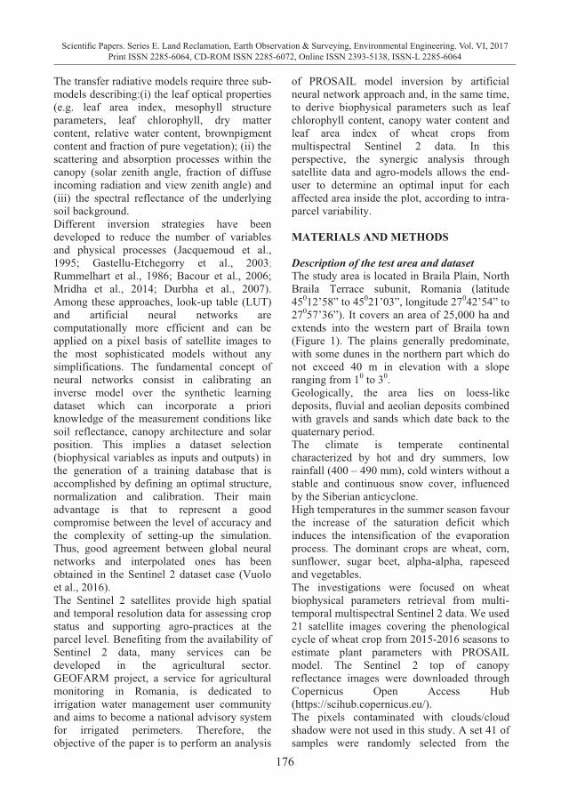
176
Scientific Papers. Series E. Land Reclamation, Earth Observation & Surveying, Environmental Engineering. Vol. VI, 2017Print ISSN 2285-6064, CD-ROM ISSN 2285-6072, Online ISSN 2393-5138, ISSN-L 2285-6064
The transfer radiative models require three sub-models describing:(i) the leaf optical properties (e.g. leaf area index, mesophyll structure parameters, leaf chlorophyll, dry matter content, relative water content, brownpigment content and fraction of pure vegetation); (ii) the scattering and absorption processes within the canopy (solar zenith angle, fraction of diffuse incoming radiation and view zenith angle) and (iii) the spectral reflectance of the underlying soil background. Different inversion strategies have been developed to reduce the number of variables and physical processes (Jacquemoud et al., 1995; Gastellu-Etchegorry et al., 2003; Rummelhart et al., 1986; Bacour et al., 2006; Mridha et al., 2014; Durbha et al., 2007). Among these approaches, look-up table (LUT) and artificial neural networks are computationally more efficient and can be applied on a pixel basis of satellite images to the most sophisticated models without any simplifications. The fundamental concept of neural networks consist in calibrating an inverse model over the synthetic learning dataset which can incorporate a priori knowledge of the measurement conditions like soil reflectance, canopy architecture and solar position. This implies a dataset selection (biophysical variables as inputs and outputs) in the generation of a training database that is accomplished by defining an optimal structure, normalization and calibration. Their main advantage is that to represent a good compromise between the level of accuracy and the complexity of setting-up the simulation. Thus, good agreement between global neural networks and interpolated ones has been obtained in the Sentinel 2 dataset case (Vuolo et al., 2016). The Sentinel 2 satellites provide high spatial and temporal resolution data for assessing crop status and supporting agro-practices at the parcel level. Benefiting from the availability of Sentinel 2 data, many services can be developed in the agricultural sector. GEOFARM project, a service for agricultural monitoring in Romania, is dedicated to irrigation water management user community and aims to become a national advisory system for irrigated perimeters. Therefore, the objective of the paper is to perform an analysis
of PROSAIL model inversion by artificial neural network approach and, in the same time, to derive biophysical parameters such as leaf chlorophyll content, canopy water content and leaf area index of wheat crops from multispectral Sentinel 2 data. In this perspective, the synergic analysis through satellite data and agro-models allows the end-user to determine an optimal input for each affected area inside the plot, according to intra-parcel variability. MATERIALS AND METHODS Description of the test area and dataset The study area is located in Braila Plain, North Braila Terrace subunit, Romania (latitude 45012’58” to 45021’03”, longitude 27042’54” to 27057’36”). It covers an area of 25,000 ha and extends into the western part of Braila town (Figure 1). The plains generally predominate, with some dunes in the northern part which do not exceed 40 m in elevation with a slope ranging from 10 to 30. Geologically, the area lies on loess-like deposits, fluvial and aeolian deposits combined with gravels and sands which date back to the quaternary period. The climate is temperate continental characterized by hot and dry summers, low rainfall (400 – 490 mm), cold winters without a stable and continuous snow cover, influenced by the Siberian anticyclone. High temperatures in the summer season favour the increase of the saturation deficit which induces the intensification of the evaporation process. The dominant crops are wheat, corn, sunflower, sugar beet, alpha-alpha, rapeseed and vegetables. The investigations were focused on wheat biophysical parameters retrieval from multi-temporal multispectral Sentinel 2 data. We used 21 satellite images covering the phenological cycle of wheat crop from 2015-2016 seasons to estimate plant parameters with PROSAIL model. The Sentinel 2 top of canopy reflectance images were downloaded through Copernicus Open Access Hub (https://scihub.copernicus.eu/). The pixels contaminated with clouds/cloud shadow were not used in this study. A set 41 of samples were randomly selected from the
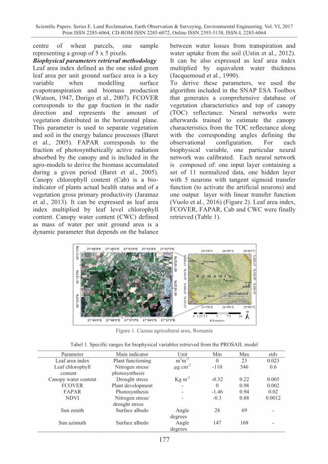
177
Scientific Papers. Series E. Land Reclamation, Earth Observation & Surveying, Environmental Engineering. Vol. VI, 2017Print ISSN 2285-6064, CD-ROM ISSN 2285-6072, Online ISSN 2393-5138, ISSN-L 2285-6064
centre of wheat parcels, one sample representing a group of 5 x 5 pixels. Biophysical parameters retrieval methodology Leaf area index defined as the one sided green leaf area per unit ground surface area is a key variable when modelling surface evapotranspiration and biomass production (Watson, 1947, Dorigo et al., 2007). FCOVER corresponds to the gap fraction in the nadir direction and represents the amount of vegetation distributed in the horizontal plane. This parameter is used to separate vegetation and soil in the energy balance processes (Baret et al., 2005). FAPAR corresponds to the fraction of photosynthetically active radiation absorbed by the canopy and is included in the agro-models to derive the biomass accumulated during a given period (Baret et al., 2005). Canopy chlorophyll content (Cab) is a bio-indicator of plants actual health status and of a vegetation gross primary productivity (Jaramaz et al., 2013). It can be expressed as leaf area index multiplied by leaf level chlorophyll content. Canopy water content (CWC) defined as mass of water per unit ground area is a dynamic parameter that depends on the balance
between water losses from transpiration and water uptake from the soil (Ustin et al., 2012). It can be also expressed as leaf area index multiplied by equivalent water thickness (Jacquemoud et al., 1990). To derive these parameters, we used the algorithm included in the SNAP ESA Toolbox that generates a comprehensive database of vegetation characteristics and top of canopy (TOC) reflectance. Neural networks were afterwards trained to estimate the canopy characteristics from the TOC reflectance along with the corresponding angles defining the observational configuration. For each biophysical variable, one particular neural network was calibrated. Each neural network is composed of: one input layer containing a set of 11 normalized data, one hidden layer with 5 neurons with tangent sigmoid transfer function (to activate the artificial neurons) and one output layer with linear transfer function (Vuolo et al., 2016) (Figure 2). Leaf area index, FCOVER, FAPAR, Cab and CWC were finally retrieved (Table 1).
Figure 1. Cazasu agricultural area, Romania
Tabel 1. Specific ranges for biophysical variables retrieved from the PROSAIL model
Parameter Main indicator Unit Min Max stdv Leaf area index Plant functioning m2m-2 0 23 0.023 Leaf chlorophyll
content Nitrogen stress/
photosynthesis µg cm-2 -110 546 0.6
Canopy water content Drought stress Kg m-2 -0.32 0.22 0.005 FCOVER Plant development - 0 0.98 0.002 FAPAR Photosynthesis - -1.46 0.94 0.02 NDVI Nitrogen stress/
drought stress - -0.3 0.88 0.0012
Sun zenith Surface albedo Angle degrees
28 69 -
Sun azimuth Surface albedo Angle degrees
147 168 -
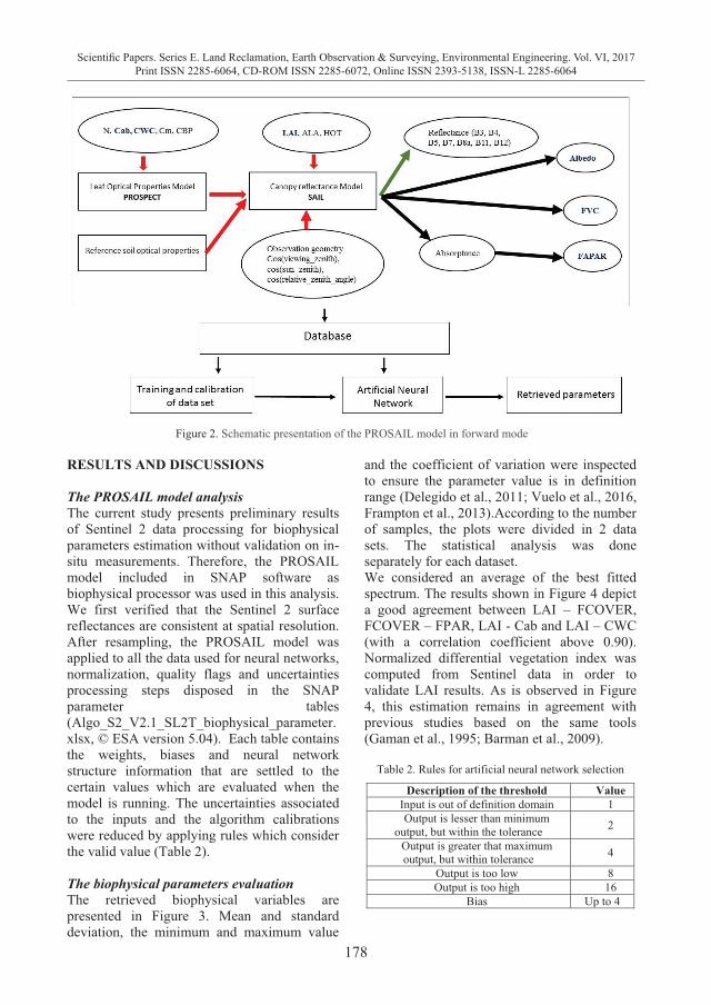
178
Scientific Papers. Series E. Land Reclamation, Earth Observation & Surveying, Environmental Engineering. Vol. VI, 2017Print ISSN 2285-6064, CD-ROM ISSN 2285-6072, Online ISSN 2393-5138, ISSN-L 2285-6064
Figure 2. Schematic presentation of the PROSAIL model in forward mode
RESULTS AND DISCUSSIONS The PROSAIL model analysis The current study presents preliminary results of Sentinel 2 data processing for biophysical parameters estimation without validation on in-situ measurements. Therefore, the PROSAIL model included in SNAP software as biophysical processor was used in this analysis. We first verified that the Sentinel 2 surface reflectances are consistent at spatial resolution. After resampling, the PROSAIL model was applied to all the data used for neural networks, normalization, quality flags and uncertainties processing steps disposed in the SNAP parameter tables (Algo_S2_V2.1_SL2T_biophysical_parameter.xlsx, © ESA version 5.04). Each table contains the weights, biases and neural network structure information that are settled to the certain values which are evaluated when the model is running. The uncertainties associated to the inputs and the algorithm calibrations were reduced by applying rules which consider the valid value (Table 2). The biophysical parameters evaluation The retrieved biophysical variables are presented in Figure 3. Mean and standard deviation, the minimum and maximum value
and the coefficient of variation were inspected to ensure the parameter value is in definition range (Delegido et al., 2011; Vuelo et al., 2016, Frampton et al., 2013).According to the number of samples, the plots were divided in 2 data sets. The statistical analysis was done separately for each dataset. We considered an average of the best fitted spectrum. The results shown in Figure 4 depict a good agreement between LAI – FCOVER, FCOVER – FPAR, LAI - Cab and LAI – CWC (with a correlation coefficient above 0.90). Normalized differential vegetation index was computed from Sentinel data in order to validate LAI results. As is observed in Figure 4, this estimation remains in agreement with previous studies based on the same tools (Gaman et al., 1995; Barman et al., 2009).
Table 2. Rules for artificial neural network selection
Description of the threshold Value Input is out of definition domain 1 Output is lesser than minimum
output, but within the tolerance 2
Output is greater that maximum output, but within tolerance 4
Output is too low 8 Output is too high 16
Bias Up to 4
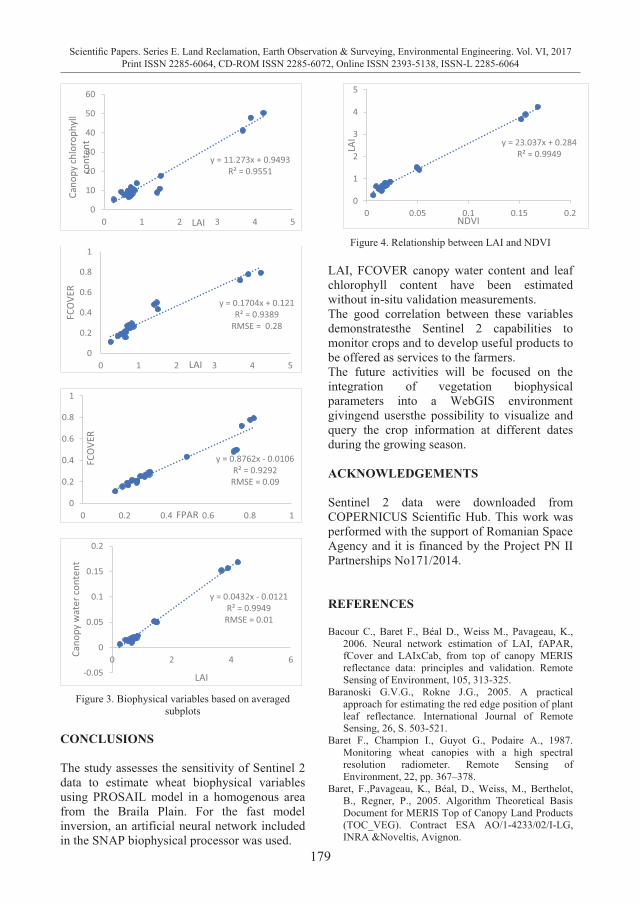
179
Scientific Papers. Series E. Land Reclamation, Earth Observation & Surveying, Environmental Engineering. Vol. VI, 2017Print ISSN 2285-6064, CD-ROM ISSN 2285-6072, Online ISSN 2393-5138, ISSN-L 2285-6064
Figure 3. Biophysical variables based on averaged
subplots CONCLUSIONS The study assesses the sensitivity of Sentinel 2 data to estimate wheat biophysical variables using PROSAIL model in a homogenous area from the Braila Plain. For the fast model inversion, an artificial neural network included in the SNAP biophysical processor was used.
Figure 4. Relationship between LAI and NDVI
LAI, FCOVER canopy water content and leaf chlorophyll content have been estimated without in-situ validation measurements. The good correlation between these variables demonstratesthe Sentinel 2 capabilities to monitor crops and to develop useful products to be offered as services to the farmers. The future activities will be focused on the integration of vegetation biophysical parameters into a WebGIS environment givingend usersthe possibility to visualize and query the crop information at different dates during the growing season.
ACKNOWLEDGEMENTS
Sentinel 2 data were downloaded from COPERNICUS Scientific Hub. This work was performed with the support of Romanian Space Agency and it is financed by the Project PN II Partnerships No171/2014.
REFERENCES
Bacour C., Baret F., Béal D., Weiss M., Pavageau, K., 2006. Neural network estimation of LAI, fAPAR, fCover and LAIxCab, from top of canopy MERIS reflectance data: principles and validation. Remote Sensing of Environment, 105, 313-325.
Baranoski G.V.G., Rokne J.G., 2005. A practical approach for estimating the red edge position of plant leaf reflectance. International Journal of Remote Sensing, 26, S. 503-521.
Baret F., Champion I., Guyot G., Podaire A., 1987. Monitoring wheat canopies with a high spectral resolution radiometer. Remote Sensing of Environment, 22, pp. 367–378.
Baret, F.,Pavageau, K., Béal, D., Weiss, M., Berthelot, B., Regner, P., 2005. Algorithm Theoretical Basis Document for MERIS Top of Canopy Land Products (TOC_VEG). Contract ESA AO/1-4233/02/I-LG, INRA &Noveltis, Avignon.
y = 11.273x + 0.9493 R² = 0.9551
0
10
20
30
40
50
60
0 1 2 3 4 5
Cano
py ch
loro
phyl
l co
nten
t
LAI
y = 0.1704x + 0.121 R² = 0.9389
RMSE = 0.28
0
0.2
0.4
0.6
0.8
1
0 1 2 3 4 5
FCO
VER
LAI
y = 0.8762x - 0.0106 R² = 0.9292
RMSE = 0.09
0
0.2
0.4
0.6
0.8
1
0 0.2 0.4 0.6 0.8 1
FCO
VER
FPAR
y = 0.0432x - 0.0121 R² = 0.9949
RMSE = 0.01
-0.05
0
0.05
0.1
0.15
0.2
0 2 4 6Cano
py w
ater
con
tent
LAI
y = 23.037x + 0.284 R² = 0.9949
0
1
2
3
4
5
0 0.05 0.1 0.15 0.2
LAI
NDVI
180
Scientific Papers. Series E. Land Reclamation, Earth Observation & Surveying, Environmental Engineering. Vol. VI, 2017Print ISSN 2285-6064, CD-ROM ISSN 2285-6072, Online ISSN 2393-5138, ISSN-L 2285-6064
Barman,,D., Kalra, N., Sahoo, R.N., Chakraborty, D., Kamble, K., 2009. Deriving Homogeneous Soil Fertility Unit through GIS for Site Specific Nutrient Management by QUEFTS model, Fourth World Congress on “Conservation Agriculture”, Feb 4-7, New Delhi, India.
Bonham-Carter G., 1988. Numerical procedures and computer program for fitting an inverted Gaussian model to vegetation reflectance data. Computers and Geosciences, 14, pp. 339–356.
Clevers J., Jongschaap R., 2001. Imaging spectrometry for agricultural applications. In Imaging Spectrometry. Basic principles and prospective applications, F. van der Meer and S. de Jong (Eds) (Dordrecht: Kluwer), pp. 157–199.
Danson F., Plummer S., 1995. Red edge response to forest leaf area index. International Journal of Remote Sensing, 16, pp. 183–188.
Dawson T.P. and Curran P.J., 1998. A new technique for interpolating red edge position. International Journal of Remote Sensing, 19(11): 2133-2139.
Delegido, J., Verrelst, J., Alonso, L., Moreno, J., 2011. Evaluation of Sentinel-2 Red-Edge Bands for Empirical Estimation of Green LAI and Chlorophyll Content. Sensors (Basel, Switzerland), 11(7), 7063–7081.
Demetriades-Shah T., Steven M.D., Clark J.A., 1990. High resolution derivative spectra in remote sensing. Remote Sensing of Environment, 33, pp. 55–64.
Dorigo, W.A.,Jurita-Milla, R., de Wit, A.J.W., Brazile, J., Singh, R., Schaepman, M.E., 2007. A review on reflective remote sensing and data assimilationtechniques for enhanced agroecosystem modeling. Int. J. Appl. Earth Obs. Geoinf. 9(2), 165–193.
Durbha S.S., King R.L., Younan N.H., 2007. Support vector machines regression for retrieval of leaf area index from multiangle imaging spectroradiometer. Remote Sens. Environ., 107:348–61.
Frampton, W. J., Dash, J.,Watmough, G., Milton, E. J., 2013. Evaluating the capabilities of Sentinel-2 for quantitative estimation of biophysical variables in vegetation, ISPRS Journal of Photogrammetry and Remote Sensing, Volume 82, 83-92.
Gamon, J.A., Field, C.B., Goulden, M.L., Griffin, K.L., 1995. Relationship between NDVI, canopy structure and photosynthesis in three California vegetation types. EcolAppl 5:28–41.
Gastellu-Etchegorry J.P., Gascon F., Esteve P., 2003. An interpolation procedure for generalizing a look-up table inversion method. Remote Sens. Environ., 87 (1), pp. 55–71.
Guyot G., Baret F. and Jacquemond S., 1992. Imaging spectroscopy for vegetation studies. In Imaging Spectrometry: Fundamentals and prospective applications, F. Toselli and J. Bodechtel (Eds) (Dordrecht: Kluwer), pp. 145–165.
Jacquemoud S., Baret F., Andrieu B., Danson F. M., Jaggard K., 1995. Extraction of vegetation biophysical parameters by inversion of the PROSPECT+SAIL model on sugar beet canopy reflectance data — Application to TM and AVIRIS
sensors. Remote Sensing of Environment, 52, 163−172.
Jacquemoud S., Verhoef W., Baret F., Bacour C., Zarco-Tejada P.J., Asner G.P., François C., Ustin S.L, 2009. PROSPECT+SAIL models: A review of use for vegetation characterization. Remote Sens. Environ., 113, 56–66.
Jacquemoud, S., Baret, F., 1990. Prospect – a model of leaf optical-properties spectra. Remote Sens Environ 34:75–91.
Jaramaz, D., Perovic, V., Belanovic, S., Saljnikov, E., Cakmak, D., Mrvic, V., Zivotic, L., 2013. The ESA Sentinel-2 mission vegetation variables for remote sensing of plant monitoring. 2nd Int. Sci. Conf. RESPAG 2013, 950-961.
Miller J.R., Hare E.W., Wu J., 1990. Quantitative characterization of the red edge reflectance. An invertedGaussian reflectance model. International Journal of Remote Sensing, 11(10): 1755-1773.
Mridha N., Sahoo R. N., Kumar D. N., Sehgal V. K., Krishna G., Pradhan S., Gupta V. K., 2014. Genetic algorithm based inversion modelling of PROSAIL for retrieval of wheat biophysical parameters from the reflectance data. J. Agric. Phys., 14(1), 87–95.
Pu R., Gong P., Biging G.S., Larrieu, M.R., 2003. Extraction of red edge optical parameters from Hyperion data for estimation of forest leaf area index. IEEE Transactions on Geoscience and Remote Sensing, 41(4): 916-921.
Rummelhart D.E., Hinton G.E., Williams R.J., 1986. Learning internal representations by error propagation. In D. Rummelhart, & J. Mc Clelland (Eds.), Parallel data processing (pp. 318-362). Cambridge, MA (USA): M.I.T. press.
Ustin, S.L., Riaño, D., Hunt, E.R., 2012. Estimating canopy water content from spectroscopy. Israel J Plant Sci 60:9–23.
Verhoef W., 1984. Light scattering by leaf layers with application to canopy reflectance modeling: The SAIL model. Remote Sensing of Environment, 16(2), 125−141.
Vuolo, F., Atzberger, C., Richter, K., D’Urso, G., Dash, J., 2010. Retrieval of biophysical vegetation products from RapidEye imagery. ISPRS TC VII Symposium – 100 Years ISPRS, vol. 38. ISPRS, Vienna, Austria, pp. 281–286.
Vuolo F., Żóltak M., Pipitone C., Zappa L., Wenng H., Immitzer M., Weiss M., Baret F., Atzberger C., 2016. Data service platform for Sentinel-2 surface reflectance and value-added products: System use and examples. Remote Sens. 2016, 8.
Thorp, K.R., Wang, G., West, A.L., Moran, M.S., Bronson, K.F., White, J.W., Mon, J., 2012. Estimating crop biophysical properties from remote sensing data by inverting linked radiative transfer and ecophysiological models. Publications from USDA-ARS / UNL Faculty, Paper 1173.
Watson, D. J., 1947. Comparative physiological studies in the growth of field crops I. Variation innet assimilation rate and leaf area between species and varieties, and within and between years.Annals of Botany, Vol. 11, pp. 41–76.
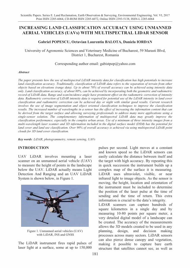
181
Scientific Papers. Series E. Land Reclamation, Earth Observation & Surveying, Environmental Engineering. Vol. VI, 2017Print ISSN 2285-6064, CD-ROM ISSN 2285-6072, Online ISSN 2393-5138, ISSN-L 2285-6064
INCREASING LAND CLASSIFICATION ACCURACY USING UNMANNED
AERIAL VEHICLES (UAVs) WITH MULTISPECTRAL LIDAR SENSOR
Gabriel POPESCU, Octavian Laurentiu BALOTA, Daniela IORDAN
University of Agronomic Sciences and Veterinary Medicine of Bucharest, 59 Marasti Blvd, District 1, Bucharest, Romania
Corresponding author email: [email protected]
Abstract The paper presents how the use of multispectral LiDAR intensity data for classification has high potentials to increase land classification accuracy. Traditionally, classification of LiDAR data refers to the separation of terrain from other objects based on elevations (range data). Up to about 70% of overall accuracy can be achieved using intensity data only. Land classification accuracy, of about 80%, can be achieved by incorporating both the geometric and radiometric record of LiDAR data. Range and scan/incidence angle have prominent effect on the radiometric correction of intensity data. Radiometric correction of LiDAR intensity data is required for potential use of the LiDAR intensity in land cover classification and radiometric correction can be achieved day or night with similar good results. Current research involves the use of image segmentation and object oriented classification techniques to improve the classification results. The increased number of wavelengths in a sensor has the effect of increasing the information content that can be derived from the target surface and allowing surveying professionals to address many more applications using a single-sensor solution. The complementary information of multispectral LiDAR data may greatly improve the classification performance, especially in the complex urban areas. Use of a minimum of three intensity images from a multi-wavelength laser scanner and 3D information included in the digital surface model (DSM) has the potential for land cover and land use classification. Over 90% of overall accuracy is achieved via using multispectral LiDAR point clouds for 3D land cover classification. Key words: LiDAR, photogrammetry, remote sensing, UAVs
INTRODUCTION UAV LiDAR involves mounting a laser scanner on an unmanned aerial vehicle (UAV) to measure the height of points in the landscape below the UAV. LiDAR actually means Light Detection And Ranging and an UAV LiDAR System is shown below, in Figure 1.
Figure 1. Unmanned aerial vehicles (UAV)
with LiDAR, INS and GNSS The LiDAR instrument fires rapid pulses of laser light at a surface, some at up to 150,000
pulses per second. Light moves at a constant and known speed so the LiDAR sensors can easily calculate the distance between itself and the target with high accuracy. By repeating this in quick succession the instrument builds up a complex map of the surface it is measuring. LiDAR uses ultraviolet, visible, or near infrared light to image objects. As the sensor is moving, the height, location and orientation of the instrument must be included to determine the position of the laser pulse at the time of sending and the time of return. This extra information is crucial to the data’s integrity. LiDAR scanners can capture hundreds of square kilometres in a single day and by measuring 10-80 points per square meter, a very detailed digital model of a landscape can be created. The accuracy of the measurements allows the 3D models created to be used in any planning, design, and decision making processes across many sectors. LiDAR sensors can also pierce dense canopy and vegetation, making it possible to capture bare earth structure that satellites cannot see, as well as
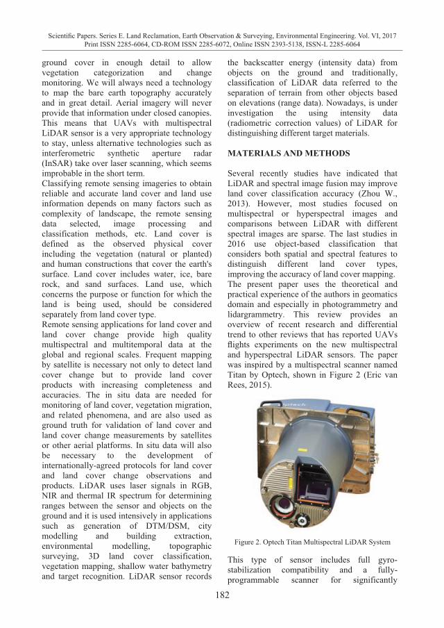
182
Scientific Papers. Series E. Land Reclamation, Earth Observation & Surveying, Environmental Engineering. Vol. VI, 2017Print ISSN 2285-6064, CD-ROM ISSN 2285-6072, Online ISSN 2393-5138, ISSN-L 2285-6064
ground cover in enough detail to allow vegetation categorization and change monitoring. We will always need a technology to map the bare earth topography accurately and in great detail. Aerial imagery will never provide that information under closed canopies. This means that UAVs with multispectral LiDAR sensor is a very appropriate technology to stay, unless alternative technologies such as interferometric synthetic aperture radar (InSAR) take over laser scanning, which seems improbable in the short term. Classifying remote sensing imageries to obtain reliable and accurate land cover and land use information depends on many factors such as complexity of landscape, the remote sensing data selected, image processing and classification methods, etc. Land cover is defined as the observed physical cover including the vegetation (natural or planted) and human constructions that cover the earth's surface. Land cover includes water, ice, bare rock, and sand surfaces. Land use, which concerns the purpose or function for which the land is being used, should be considered separately from land cover type. Remote sensing applications for land cover and land cover change provide high quality multispectral and multitemporal data at the global and regional scales. Frequent mapping by satellite is necessary not only to detect land cover change but to provide land cover products with increasing completeness and accuracies. The in situ data are needed for monitoring of land cover, vegetation migration, and related phenomena, and are also used as ground truth for validation of land cover and land cover change measurements by satellites or other aerial platforms. In situ data will also be necessary to the development of internationally-agreed protocols for land cover and land cover change observations and products. LiDAR uses laser signals in RGB, NIR and thermal IR spectrum for determining ranges between the sensor and objects on the ground and it is used intensively in applications such as generation of DTM/DSM, city modelling and building extraction, environmental modelling, topographic surveying, 3D land cover classification, vegetation mapping, shallow water bathymetry and target recognition. LiDAR sensor records
the backscatter energy (intensity data) from objects on the ground and traditionally, classification of LiDAR data referred to the separation of terrain from other objects based on elevations (range data). Nowadays, is under investigation the using intensity data (radiometric correction values) of LiDAR for distinguishing different target materials. MATERIALS AND METHODS Several recently studies have indicated that LiDAR and spectral image fusion may improve land cover classification accuracy (Zhou W., 2013). However, most studies focused on multispectral or hyperspectral images and comparisons between LiDAR with different spectral images are sparse. The last studies in 2016 use object-based classification that considers both spatial and spectral features to distinguish different land cover types, improving the accuracy of land cover mapping. The present paper uses the theoretical and practical experience of the authors in geomatics domain and especially in photogrammetry and lidargrammetry. This review provides an overview of recent research and differential trend to other reviews that has reported UAVs flights experiments on the new multispectral and hyperspectral LiDAR sensors. The paper was inspired by a multispectral scanner named Titan by Optech, shown in Figure 2 (Eric van Rees, 2015).
Figure 2. Optech Titan Multispectral LiDAR System This type of sensor includes full gyro-stabilization compatibility and a fully-programmable scanner for significantly
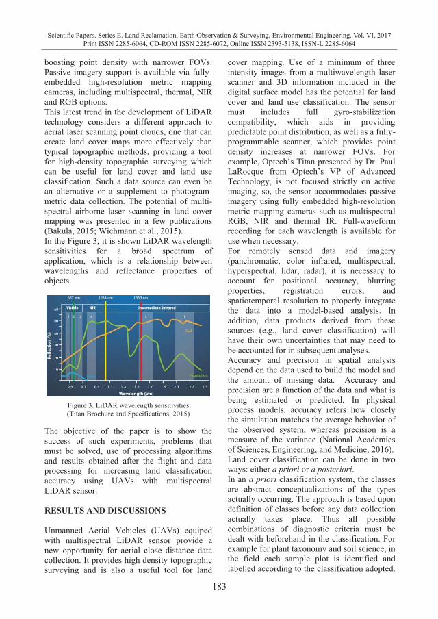
183
Scientific Papers. Series E. Land Reclamation, Earth Observation & Surveying, Environmental Engineering. Vol. VI, 2017Print ISSN 2285-6064, CD-ROM ISSN 2285-6072, Online ISSN 2393-5138, ISSN-L 2285-6064
boosting point density with narrower FOVs. Passive imagery support is available via fully-embedded high-resolution metric mapping cameras, including multispectral, thermal, NIR and RGB options. This latest trend in the development of LiDAR technology considers a different approach to aerial laser scanning point clouds, one that can create land cover maps more effectively than typical topographic methods, providing a tool for high-density topographic surveying which can be useful for land cover and land use classification. Such a data source can even be an alternative or a supplement to photogram-metric data collection. The potential of multi-spectral airborne laser scanning in land cover mapping was presented in a few publications (Bakula, 2015; Wichmann et al., 2015). In the Figure 3, it is shown LiDAR wavelength sensitivities for a broad spectrum of application, which is a relationship between wavelengths and reflectance properties of objects.
Figure 3. LiDAR wavelength sensitivities (Titan Brochure and Specifications, 2015)
The objective of the paper is to show the success of such experiments, problems that must be solved, use of processing algorithms and results obtained after the flight and data processing for increasing land classification accuracy using UAVs with multispectral LiDAR sensor. RESULTS AND DISCUSSIONS Unmanned Aerial Vehicles (UAVs) equiped with multispectral LiDAR sensor provide a new opportunity for aerial close distance data collection. It provides high density topographic surveying and is also a useful tool for land
cover mapping. Use of a minimum of three intensity images from a multiwavelength laser scanner and 3D information included in the digital surface model has the potential for land cover and land use classification. The sensor must includes full gyro-stabilization compatibility, which aids in providing predictable point distribution, as well as a fully-programmable scanner, which provides point density increases at narrower FOVs. For example, Optech’s Titan presented by Dr. Paul LaRocque from Optech’s VP of Advanced Technology, is not focused strictly on active imaging, so, the sensor accommodates passive imagery using fully embedded high-resolution metric mapping cameras such as multispectral RGB, NIR and thermal IR. Full-waveform recording for each wavelength is available for use when necessary. For remotely sensed data and imagery (panchromatic, color infrared, multispectral, hyperspectral, lidar, radar), it is necessary to account for positional accuracy, blurring properties, registration errors, and spatiotemporal resolution to properly integrate the data into a model-based analysis. In addition, data products derived from these sources (e.g., land cover classification) will have their own uncertainties that may need to be accounted for in subsequent analyses. Accuracy and precision in spatial analysis depend on the data used to build the model and the amount of missing data. Accuracy and precision are a function of the data and what is being estimated or predicted. In physical process models, accuracy refers how closely the simulation matches the average behavior of the observed system, whereas precision is a measure of the variance (National Academies of Sciences, Engineering, and Medicine, 2016). Land cover classification can be done in two ways: either a priori or a posteriori. In an a priori classification system, the classes are abstract conceptualizations of the types actually occurring. The approach is based upon definition of classes before any data collection actually takes place. Thus all possible combinations of diagnostic criteria must be dealt with beforehand in the classification. For example for plant taxonomy and soil science, in the field each sample plot is identified and labelled according to the classification adopted.
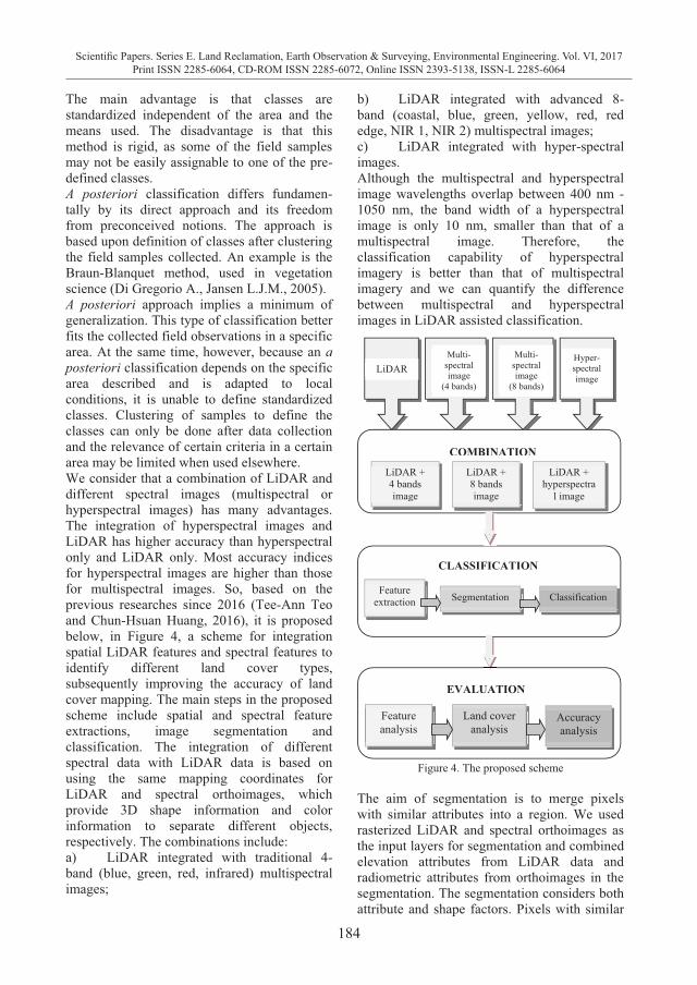
184
Scientific Papers. Series E. Land Reclamation, Earth Observation & Surveying, Environmental Engineering. Vol. VI, 2017Print ISSN 2285-6064, CD-ROM ISSN 2285-6072, Online ISSN 2393-5138, ISSN-L 2285-6064
The main advantage is that classes are standardized independent of the area and the means used. The disadvantage is that this method is rigid, as some of the field samples may not be easily assignable to one of the pre-defined classes. A posteriori classification differs fundamen-tally by its direct approach and its freedom from preconceived notions. The approach is based upon definition of classes after clustering the field samples collected. An example is the Braun-Blanquet method, used in vegetation science (Di Gregorio A., Jansen L.J.M., 2005). A posteriori approach implies a minimum of generalization. This type of classification better fits the collected field observations in a specific area. At the same time, however, because an a posteriori classification depends on the specific area described and is adapted to local conditions, it is unable to define standardized classes. Clustering of samples to define the classes can only be done after data collection and the relevance of certain criteria in a certain area may be limited when used elsewhere. We consider that a combination of LiDAR and different spectral images (multispectral or hyperspectral images) has many advantages. The integration of hyperspectral images and LiDAR has higher accuracy than hyperspectral only and LiDAR only. Most accuracy indices for hyperspectral images are higher than those for multispectral images. So, based on the previous researches since 2016 (Tee-Ann Teo and Chun-Hsuan Huang, 2016), it is proposed below, in Figure 4, a scheme for integration spatial LiDAR features and spectral features to identify different land cover types, subsequently improving the accuracy of land cover mapping. The main steps in the proposed scheme include spatial and spectral feature extractions, image segmentation and classification. The integration of different spectral data with LiDAR data is based on using the same mapping coordinates for LiDAR and spectral orthoimages, which provide 3D shape information and color information to separate different objects, respectively. The combinations include: a) LiDAR integrated with traditional 4-band (blue, green, red, infrared) multispectral images;
b) LiDAR integrated with advanced 8-band (coastal, blue, green, yellow, red, red edge, NIR 1, NIR 2) multispectral images; c) LiDAR integrated with hyper-spectral images. Although the multispectral and hyperspectral image wavelengths overlap between 400 nm -1050 nm, the band width of a hyperspectral image is only 10 nm, smaller than that of a multispectral image. Therefore, the classification capability of hyperspectral imagery is better than that of multispectral imagery and we can quantify the difference between multispectral and hyperspectral images in LiDAR assisted classification.
Figure 4. The proposed scheme
The aim of segmentation is to merge pixels with similar attributes into a region. We used rasterized LiDAR and spectral orthoimages as the input layers for segmentation and combined elevation attributes from LiDAR data and radiometric attributes from orthoimages in the segmentation. The segmentation considers both attribute and shape factors. Pixels with similar
LiDAR Multi-
spectral image
(4 bands)
Multi-spectral image
(8 bands)
Hyper-spectral image
COMBINATION
LiDAR + 4 bands image
LiDAR + 8 bands image
LiDAR + hyperspectra
l image
CLASSIFICATION
Feature extraction Segmentation Classification
EVALUATION
Feature analysis
Land cover analysis
Accuracy analysis
185
Scientific Papers. Series E. Land Reclamation, Earth Observation & Surveying, Environmental Engineering. Vol. VI, 2017Print ISSN 2285-6064, CD-ROM ISSN 2285-6072, Online ISSN 2393-5138, ISSN-L 2285-6064
height and spectral attributes are merged into a region. The attribute is the pixel value of the input layer whereas the shape factor is the shape of the segmented object. The segment concept is based on the heterogeneity index, expressed in equation 1. The heterogeneity combines the attribute (expressed in equation 2) and shape (expressed in equation 3) factors. The segmentation is a bottom up method that starts from a pixel. Each pixel is treated as a small object and neighbourhood pixels are added to calculate the heterogeneity index. If the heterogeneity index meets the predefined criterion, these pixels are merged together (Tee-Ann Teo and Chun-Hsuan Huang, 2016).
h = wattribute * hattribute + wshape* hshape (1) hattribute = � wi �i , unde i=1…n (2) hshape = wsmoothness * hsmoothness + + wcompactness * h compactness (3) hsmoothness = l/b hcompactness = l/ n
where:
h is heterogeneity index; hattribute and hshape are attribute and shape indices; wattribute and wshape are weights; wattribute + wshape = 1; wi is weight for layer i; σi is the standard deviation of layer i; hsmoothness and hcompactness are smoothness and compactness indices, respectively, for shape; l is perimeter; b is smaller length of size; and n is area.
In general, the advantages of this method are that the different layers have different weights and the segmentation considers the attribute (pixel value) and also the shape of objects. After segmentation, an object-based classification rather than pixel-based classification is performed. Each separated region after segmentation is a candidate object for classification. An object-based classification considering the characteristics of elevation, spectral, texture, roughness, and shape information is performed to separate different land cover types. The object based
image analysis approach is an effective way to classify the multispectral LiDAR point clouds data for 3D land cover classification. The definition of classification indexes is very attractive for the separation of different height vegetation and spectral similar objects point clouds. Repeating the segmentation with different scale parameters make the boundaries of 3D land cover types distinguish from other objects features easily. For evaluating the classification results, confusion matrix and error statistics for nine classes must be calcu-lated, and overall accuracy obtained should be over 91% (Zou Xiaoliang et al., 2016). Multispectral LiDAR point clouds are segmented and classified on the basis of return signal intensity images from more than three channels raw data. The intensity depends on the reflectance of the ground material and laser pulse wavelength. Numbers of all returns point clouds, and elevation information from maximum first returns and minimum last returns are main factors for classification. Meanwhile, different objects reflective characteristic in three channels are taken into account for classification. Water is best penetrated in green spectrum, and a slightly reflective in NIR and IR spectrum. Power line is strongly reflective in NIR and IR spectrum and slightly reflective in green spectrum. Vegetation is strongly reflective in NIR spectrum, and slightly reflective in visible green spectrum. Soil is best reflective in intermediate IR and vegetation can be easily distinguished from soil and water. After the image objects classification of multispectral point clouds, is performed the accuracy assessment by comparing randomly distributed sampled points in reference imagery with the classification results. The reference points are compared with classification results at the same locations. We use these known reference points to assess the validity of the classification results, to calculate a confusion matrix, to derive the user’s accuracy and producer’s accuracy for each class, to calculate errors of commission and omission for each class, and to compute an overall accuracy and kappa statistics for the classification results. The accuracy of the image based point cloud can be evaluated using precisely measured ground reference points. So, the dense
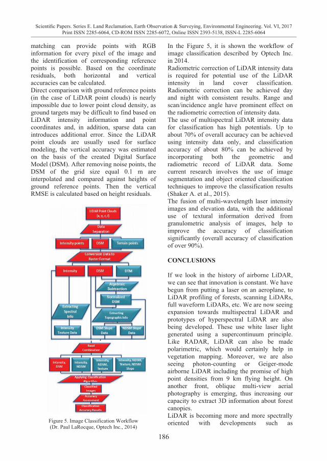
186
Scientific Papers. Series E. Land Reclamation, Earth Observation & Surveying, Environmental Engineering. Vol. VI, 2017Print ISSN 2285-6064, CD-ROM ISSN 2285-6072, Online ISSN 2393-5138, ISSN-L 2285-6064
matching can provide points with RGB information for every pixel of the image and the identification of corresponding reference points is possible. Based on the coordinate residuals, both horizontal and vertical accuracies can be calculated. Direct comparison with ground reference points (in the case of LiDAR point clouds) is nearly impossible due to lower point cloud density, as ground targets may be difficult to find based on LiDAR intensity information and point coordinates and, in addition, sparse data can introduces additional error. Since the LiDAR point clouds are usually used for surface modeling, the vertical accuracy was estimated on the basis of the created Digital Surface Model (DSM). After removing noise points, the DSM of the grid size equal 0.1 m are interpolated and compared against heights of ground reference points. Then the vertical RMSE is calculated based on height residuals.
Figure 5. Image Classification Workflow (Dr. Paul LaRocque, Optech Inc., 2014)
In the Figure 5, it is shown the workflow of image classification described by Optech Inc. in 2014. Radiometric correction of LiDAR intensity data is required for potential use of the LiDAR intensity in land cover classification. Radiometric correction can be achieved day and night with consistent results. Range and scan/incidence angle have prominent effect on the radiometric correction of intensity data. The use of multispectral LiDAR intensity data for classification has high potentials. Up to about 70% of overall accuracy can be achieved using intensity data only, and classification accuracy of about 80% can be achieved by incorporating both the geometric and radiometric record of LiDAR data. Some current research involves the use of image segmentation and object oriented classification techniques to improve the classification results (Shaker A. et al., 2015). The fusion of multi-wavelength laser intensity images and elevation data, with the additional use of textural information derived from granulometric analysis of images, help to improve the accuracy of classification significantly (overall accuracy of classification of over 90%). CONCLUSIONS If we look in the history of airborne LiDAR, we can see that innovation is constant. We have begun from putting a laser on an aeroplane, to LiDAR profiling of forests, scanning LiDARs, full waveform LiDARs, etc. We are now seeing expansion towards multispectral LiDAR and prototypes of hyperspectral LiDAR are also being developed. These use white laser light generated using a supercontinuum principle. Like RADAR, LiDAR can also be made polarimetric, which would certainly help in vegetation mapping. Moreover, we are also seeing photon-counting or Geiger-mode airborne LiDAR including the promise of high point densities from 9 km flying height. On another front, oblique multi-view aerial photography is emerging, thus increasing our capacity to extract 3D information about forest canopies. LiDAR is becoming more and more spectrally oriented with developments such as
187
Scientific Papers. Series E. Land Reclamation, Earth Observation & Surveying, Environmental Engineering. Vol. VI, 2017Print ISSN 2285-6064, CD-ROM ISSN 2285-6072, Online ISSN 2393-5138, ISSN-L 2285-6064
multispectral LiDAR and imagery is moving towards better 3D extraction capabilities using multi-view oblique imagery. For these reasons, we think that both, multispectral LiDAR and imagery, will have a dense matching thriving side by side for the next decade. Multispectral LiDAR is a very recent development that may help with vegetation classification. For example, tree species information is not only necessary for timber inventory but also for habitat studies and other analysis. While LiDAR has been extremely useful for mapping forest structure, its use for species identification is still marginal. Although 3D data contains information for distinguishing species to some extent, a lot of discriminating power comes from the analysis of spectral signatures of color imagery. Tree foliage color in the visible and infrared band indeed differs between certain species. However, the radiometric corrections necessary to attenuate the variation in the sun-object-sensor geometry in airborne images are very complex. Multispectral LiDAR provides a way to measure multichannel intensities with a constant geometry, which make them easier to correct. Multispectral LiDAR system is a new promising research domain, especially in applications of 3D land cover classification, seamless shallow water bathymetry, forest inventory and vegetative classification, disaster response and topographic mapping. Further research is needed to combine multispectral LiDAR point clouds with other ancillary data such as digital surface model (DSM) and imagery in order to improve the associated precision. For example, multispectral imaging sensors on agricultural drones will allow the farmer manage crops and soil more effectively. This multispectral imaging agriculture remote sensing technology use Green, Red, Red-Edge and NIR wavebands to capture both visible and invisible images of crops and vegetation. LiDAR, multispectral and photogrammetry imagery will be all very closely related technologies. In some sectors and situations, images from all 3 are required to give a full analysis of the terrain, vegetation or structure. Both land cover spectral information and 3D surface information can be obtained efficiently via remote sensing technologies applied to
UAVs at close range domain. Spectral images provide spectral features whereas LiDAR point clouds contain 3D spatial features. Therefore, the multisensory data can be integrated to obtain useful information for different applications. This study integrates LiDAR with different spectral features for land cover classification. Because different spectral images have different characteristics, is better to use hyperspectral images or multispectral images, to distinguish different land covers. The main works include features selection, object-based classification, and evaluation. In features selection appropriate features must be selected according to the land cover characteristics. Object-based classification must be implemented using image segmentation and supervised classification. Finally, different combinations must be evaluated, using reference data to provide comprehensive analyses. We can conclude with the following three considerations, demonstrated practically by Tee-Ann Teo and Chun-Hsuan Huang in 2016: a) The integration of hyperspectral images and
LiDAR has higher accuracy than hyperspectral only and LiDAR only. The improvement rate reached 6% for the data fusion approach. The combination of spatial and spectral data is beneficial for land cover identification;
b) For the comparison of traditional 4-band and advanced 8-band multispectral images in data fusion the improvement rate of 8-band images reached 9% for 12 classes. The additional coastal, yellow, red edge, and NIR2 are useful for land cover mapping. The additional bands lead to improvement in the classification accuracies for areca, crop, and bare ground ;
c) LiDAR features are useful for separating man-made objects and vegetation, whereas spectral features are useful for separating different vegetation types. In the 8-band multispectral images comparison with hyperspectral images, using narrow hyperspectral bands has better accuracy than broad spectral bands in species classification. The improvement rate of hyperspectral images reached 13% for 12 classes.
188
Scientific Papers. Series E. Land Reclamation, Earth Observation & Surveying, Environmental Engineering. Vol. VI, 2017Print ISSN 2285-6064, CD-ROM ISSN 2285-6072, Online ISSN 2393-5138, ISSN-L 2285-6064
Custom land cover measurement products will continue to be important in satisfying the needs of the wide range of land cover data users, and the development of an integrated set of land cover measurements, that encompasses individual mission-specific land cover products, will be necessary to address the many gaps and inconsistencies that hinder comprehensive data analysis and forecasting. Validation should be an inherent part of every land cover research effort for satellite data. While satellite data must be verified by in situ measurements, the multispectral LiDAR data captured with UAVs, from an altitude of 50-100 m, are themselves in situ data for others satellite data. Probability-based sampling design provides accuracy measurements that allow the user to understand the magnitude of error. In the future, we believe that the use of UAVs will extend globally to non-urban areas. The ground control points currently used for improving geolocation mapping will be a network of sensors spread over fields and collaborating with remote sensing tasks. While today the processing of data acquired by the UAV is usually performed offline, in the future online data processing and intercommunication functionality will provide aerial works with the ability to further extend from current mapping and modelling applications to more intelligent application activities. The use of multiple laser diodes in one sensor may be potentially beneficial in refinement of the UAV’s attitude and this approach needs further algorithmic developments. In the same time, it is necessary to test in the future research new technologies and algorithms for increasing accuracies for direct and indirect geo-referencing of the multispectral / hyperspectral LiDAR and image point clouds obtained by UAVs equipped with GNSS/ IMU/Sensors (Popescu G. et al., 2015). ACKNOWLEDGEMENTS The authors would like to thank Teledyne Optech Inc. for free access to documentation material about the multispectral Lidar system Optech Titan.This review work was carried out
with the support of the laboratories of photogrammetry, remote sensing and mapping from the framework of the University of Agronomic Sciences and Veterinary Medicine of Bucharest. REFERENCES Bakula, K., 2015. Multispectral airborne laser scanning -
a new trend in the development of LiDAR technology, Archiwum Fotogrametrii, Kartografii i Teledetekcji, 27, pp. 25-44.
Di Gregorio A., Jansen L.J.M., 2005. Land Cover Classification System. Classification concepts and user manual. Software version 2. ISBN: 92-5-105327-8, FAO, Rome, Italy.
National Academies of Sciences, Engineering, and Medicine. 2016. From Maps to Models: Augmenting the Nation’s Geospatial Intelligence Capabilities. Washington DC, USA, The National Academies Press, pp 134. DOI: 10.17226/23650.
Popescu, G., Balota, O.L., Iordan, D., 2015. Direct georeferencing application of aerial photogrammetry using a GNSS/IMU/SENSOR System. Albena, Bulgaria, 18-24 iunie 2015, SGEM Conference Proceedings ISBN: 978-619-7105-34-6 / ISSN 1314-2704 , Book 2 Vol.1, pp 1043-1050.
Shaker, A., LaRocque, P., Smith, B., 2015. The Optech Titan: A Multi-Spectral Lidar for Multiple Applications. JALBTCX Workshop, 12 March 2016, pp. 1-56.
Tee-Ann Teo, Chun-Hsuan Huang, 2016. Terr. Atmos. Ocean. Sci., Vol. 27, No. 4, pp. 491-504, DOI: 10.3319/TAO. 2016.01.29.01(ISRS), August 2016.
Titan Brochure and Specifications, 2015. Optech Titan Multispectral Lidar System - High Precision Environmental Mapping, pp. 1-8.
Van Rees, E., 2015. Optech Titan, the world´s first multispectral airborne lidar sensor. GEOInformatics Magazine No.1, 2015, Vol.18, pp.10-13.
Wichmann, V., Bremer, M., Lindenberger, J., Rutzinger M., Georges, C. and Petrini-Monteferri, F., 2015. Evaluating the Potential of Mutispectral Airborne Lidar for Topographic Mapping and Land Cover Classification. ISPRS Annals of the Photogrammetry, Remote Sensing and Spatial Information Sciences, Volume II-3/W5, ISPRS Geospatial Week 2015, La Grande Motte, France, pp. 113-119.
Zhou, W., 2013. An object-based approach for urban land cover classification: integrating LiDAR height and intensity data. IEEE Geoscience and Remote Sensing Letters, Volume 10, Issue: 4, July 2013, pp. 928 – 931.
Zou X., Zhao G., Yang Y., Fang Y., 2016. 3D land cover classification based on multispectral lidar point clouds, XXIII ISPRS Congress, Prague, Czech Republic, July 12–19, 2016.
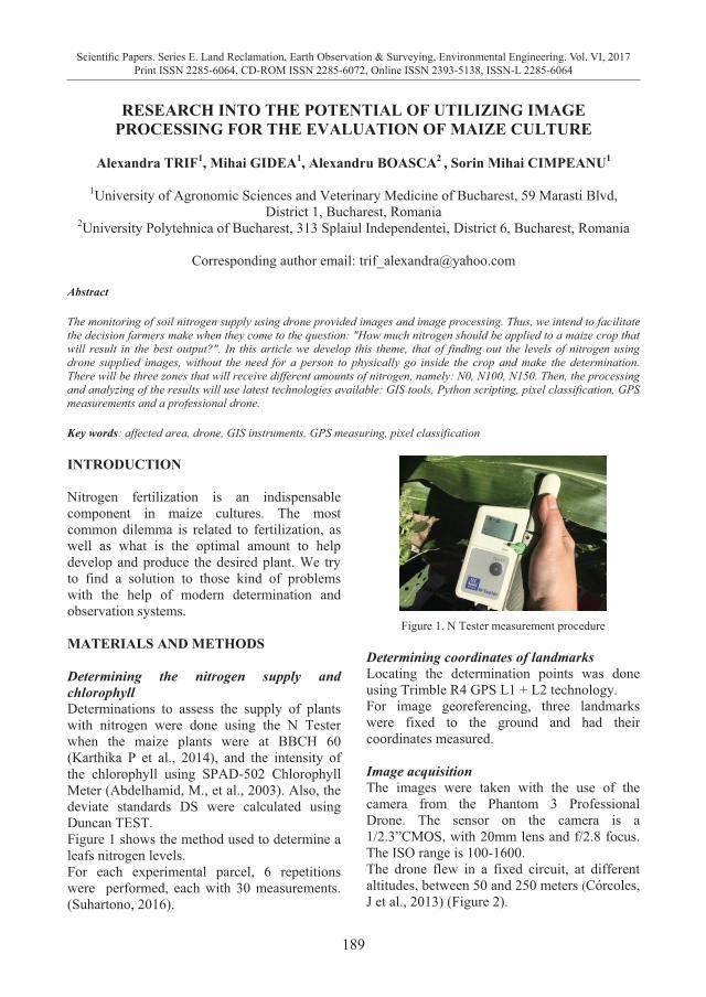
189
Scientific Papers. Series E. Land Reclamation, Earth Observation & Surveying, Environmental Engineering. Vol. VI, 2017Print ISSN 2285-6064, CD-ROM ISSN 2285-6072, Online ISSN 2393-5138, ISSN-L 2285-6064
Custom land cover measurement products will continue to be important in satisfying the needs of the wide range of land cover data users, and the development of an integrated set of land cover measurements, that encompasses individual mission-specific land cover products, will be necessary to address the many gaps and inconsistencies that hinder comprehensive data analysis and forecasting. Validation should be an inherent part of every land cover research effort for satellite data. While satellite data must be verified by in situ measurements, the multispectral LiDAR data captured with UAVs, from an altitude of 50-100 m, are themselves in situ data for others satellite data. Probability-based sampling design provides accuracy measurements that allow the user to understand the magnitude of error. In the future, we believe that the use of UAVs will extend globally to non-urban areas. The ground control points currently used for improving geolocation mapping will be a network of sensors spread over fields and collaborating with remote sensing tasks. While today the processing of data acquired by the UAV is usually performed offline, in the future online data processing and intercommunication functionality will provide aerial works with the ability to further extend from current mapping and modelling applications to more intelligent application activities. The use of multiple laser diodes in one sensor may be potentially beneficial in refinement of the UAV’s attitude and this approach needs further algorithmic developments. In the same time, it is necessary to test in the future research new technologies and algorithms for increasing accuracies for direct and indirect geo-referencing of the multispectral / hyperspectral LiDAR and image point clouds obtained by UAVs equipped with GNSS/ IMU/Sensors (Popescu G. et al., 2015). ACKNOWLEDGEMENTS The authors would like to thank Teledyne Optech Inc. for free access to documentation material about the multispectral Lidar system Optech Titan.This review work was carried out
with the support of the laboratories of photogrammetry, remote sensing and mapping from the framework of the University of Agronomic Sciences and Veterinary Medicine of Bucharest. REFERENCES Bakula, K., 2015. Multispectral airborne laser scanning -
a new trend in the development of LiDAR technology, Archiwum Fotogrametrii, Kartografii i Teledetekcji, 27, pp. 25-44.
Di Gregorio A., Jansen L.J.M., 2005. Land Cover Classification System. Classification concepts and user manual. Software version 2. ISBN: 92-5-105327-8, FAO, Rome, Italy.
National Academies of Sciences, Engineering, and Medicine. 2016. From Maps to Models: Augmenting the Nation’s Geospatial Intelligence Capabilities. Washington DC, USA, The National Academies Press, pp 134. DOI: 10.17226/23650.
Popescu, G., Balota, O.L., Iordan, D., 2015. Direct georeferencing application of aerial photogrammetry using a GNSS/IMU/SENSOR System. Albena, Bulgaria, 18-24 iunie 2015, SGEM Conference Proceedings ISBN: 978-619-7105-34-6 / ISSN 1314-2704 , Book 2 Vol.1, pp 1043-1050.
Shaker, A., LaRocque, P., Smith, B., 2015. The Optech Titan: A Multi-Spectral Lidar for Multiple Applications. JALBTCX Workshop, 12 March 2016, pp. 1-56.
Tee-Ann Teo, Chun-Hsuan Huang, 2016. Terr. Atmos. Ocean. Sci., Vol. 27, No. 4, pp. 491-504, DOI: 10.3319/TAO. 2016.01.29.01(ISRS), August 2016.
Titan Brochure and Specifications, 2015. Optech Titan Multispectral Lidar System - High Precision Environmental Mapping, pp. 1-8.
Van Rees, E., 2015. Optech Titan, the world´s first multispectral airborne lidar sensor. GEOInformatics Magazine No.1, 2015, Vol.18, pp.10-13.
Wichmann, V., Bremer, M., Lindenberger, J., Rutzinger M., Georges, C. and Petrini-Monteferri, F., 2015. Evaluating the Potential of Mutispectral Airborne Lidar for Topographic Mapping and Land Cover Classification. ISPRS Annals of the Photogrammetry, Remote Sensing and Spatial Information Sciences, Volume II-3/W5, ISPRS Geospatial Week 2015, La Grande Motte, France, pp. 113-119.
Zhou, W., 2013. An object-based approach for urban land cover classification: integrating LiDAR height and intensity data. IEEE Geoscience and Remote Sensing Letters, Volume 10, Issue: 4, July 2013, pp. 928 – 931.
Zou X., Zhao G., Yang Y., Fang Y., 2016. 3D land cover classification based on multispectral lidar point clouds, XXIII ISPRS Congress, Prague, Czech Republic, July 12–19, 2016.
RESEARCH INTO THE POTENTIAL OF UTILIZING IMAGE
PROCESSING FOR THE EVALUATION OF MAIZE CULTURE
Alexandra TRIF1, Mihai GIDEA1, Alexandru BOASCA2 , Sorin Mihai CIMPEANU1
1University of Agronomic Sciences and Veterinary Medicine of Bucharest, 59 Marasti Blvd, District 1, Bucharest, Romania
2University Polytehnica of Bucharest, 313 Splaiul Independentei, District 6, Bucharest, Romania
Corresponding author email: [email protected]
Abstract The monitoring of soil nitrogen supply using drone provided images and image processing. Thus, we intend to facilitate the decision farmers make when they come to the question: "How much nitrogen should be applied to a maize crop that will result in the best output?". In this article we develop this theme, that of finding out the levels of nitrogen using drone supplied images, without the need for a person to physically go inside the crop and make the determination. There will be three zones that will receive different amounts of nitrogen, namely: N0, N100, N150. Then, the processing and analyzing of the results will use latest technologies available: GIS tools, Python scripting, pixel classification, GPS measurements and a professional drone. Key words: affected area, drone, GIS instruments, GPS measuring, pixel classification INTRODUCTION Nitrogen fertilization is an indispensable component in maize cultures. The most common dilemma is related to fertilization, as well as what is the optimal amount to help develop and produce the desired plant. We try to find a solution to those kind of problems with the help of modern determination and observation systems. MATERIALS AND METHODS Determining the nitrogen supply and chlorophyll Determinations to assess the supply of plants with nitrogen were done using the N Tester when the maize plants were at BBCH 60 (Karthika P et al., 2014), and the intensity of the chlorophyll using SPAD-502 Chlorophyll Meter (Abdelhamid, M., et al., 2003). Also, the deviate standards DS were calculated using Duncan TEST. Figure 1 shows the method used to determine a leafs nitrogen levels. For each experimental parcel, 6 repetitions were performed, each with 30 measurements. (Suhartono, 2016).
Figure 1. N Tester measurement procedure
Determining coordinates of landmarks Locating the determination points was done using Trimble R4 GPS L1 + L2 technology. For image georeferencing, three landmarks were fixed to the ground and had their coordinates measured. Image acquisition The images were taken with the use of the camera from the Phantom 3 Professional Drone. The sensor on the camera is a 1/2.3”CMOS, with 20mm lens and f/2.8 focus. The ISO range is 100-1600. The drone flew in a fixed circuit, at different altitudes, between 50 and 250 meters (Córcoles, J et al., 2013) (Figure 2).
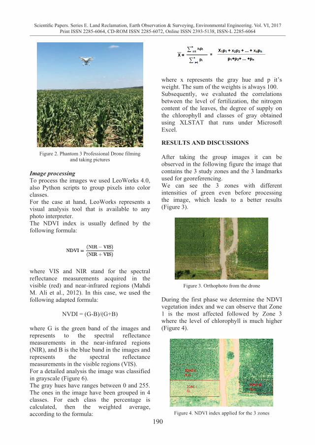
190
Scientific Papers. Series E. Land Reclamation, Earth Observation & Surveying, Environmental Engineering. Vol. VI, 2017Print ISSN 2285-6064, CD-ROM ISSN 2285-6072, Online ISSN 2393-5138, ISSN-L 2285-6064
Figure 2. Phantom 3 Professional Drone filming
and taking pictures Image processing To process the images we used LeoWorks 4.0, also Python scripts to group pixels into color classes. For the case at hand, LeoWorks represents a visual analysis tool that is available to any photo interpreter.The NDVI index is usually defined by the following formula:
where VIS and NIR stand for the spectral reflectance measurements acquired in the visible (red) and near-infrared regions (Mahdi M. Ali et al., 2012). In this case, we used the following adapted formula:
NVDI = (G-B)/(G+B)
where G is the green band of the images and represents to the spectral reflectance measurements in the near-infrared regions (NIR), and B is the blue band in the images and represents the spectral reflectance measurements in the visible regions (VIS). For a detailed analysis the image was classified in grayscale (Figure 6). The gray hues have ranges between 0 and 255. The ones in the image have been grouped in 4 classes. For each class the percentage is calculated, then the weighted average, according to the formula:
where x represents the gray hue and p it’s weight. The sum of the weights is always 100. Subsequently, we evaluated the correlations between the level of fertilization, the nitrogen content of the leaves, the degree of supply on the chlorophyll and classes of gray obtained using XLSTAT that runs under Microsoft Excel. RESULTS AND DISCUSSIONS After taking the group images it can be observed in the following figure the image that contains the 3 study zones and the 3 landmarks used for georeferencing. We can see the 3 zones with different intensities of green even before processing the image, which leads to a better results (Figure 3).
Figure 3. Orthophoto from the drone During the first phase we determine the NDVI vegetation index and we can observe that Zone 1 is the most affected followed by Zone 3 where the level of chlorophyll is much higher (Figure 4).
Figure 4. NDVI index applied for the 3 zones
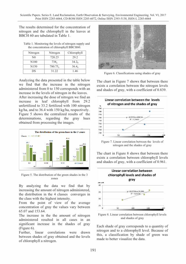
191
Scientific Papers. Series E. Land Reclamation, Earth Observation & Surveying, Environmental Engineering. Vol. VI, 2017Print ISSN 2285-6064, CD-ROM ISSN 2285-6072, Online ISSN 2393-5138, ISSN-L 2285-6064
The results determined for the concentration of nitrogen and the chlorophyll in the leaves at BBCH 60 are tabulated in Table 1.
Table 1. Monitoring the levels of nitrogen supply and the concentration of chlorophyll BBCH60.
Nitrogen Nitrogen Chlorophyll N0 720.25 29.2
N100 738a 34.2b N150 780.75a 36.4a DS 31.22 1.46
Analyzing the data presented in the table below we find that the increase in the nitrogen administered from 0 to 150 corresponds with an increase in the levels of nitrogen in the leaves. After increasing the dose of nitrogen we find an increase in leaf chlorophyll from 29.2 unfertilized to 33.2 fertilized with 100 nitrogen kg/ha, and to 36.4 with 150 kg/ha, respectively. Figure 5 shows the centralized results of the determinations, regarding the gray hues obtained from processing the images.
Figure 5. The distribution of the green shades in the 3
zones By analyzing the data we find that by increasing the amount of nitrogen administered, the distribution in the 4 classes converges in the class with the highest intensity. From the point of view of the average concentration of gray the values vary between 65.07 and 153.64. The increase in the the amount of nitrogen administered resulted in all cases in an significant increase in the shades of gray (Figure 6). Further, linear correlations were drawn between shades of gray obtained and the levels of chlorophyll a nitrogen.
Figure 6. Classifications using shades of gray
The chart in Figure 7 shows that between there exists a correlation between the nitrogen levels and shades of gray, with a coefficient of 0.839.
Figure 7. Linear correlation between the levels of
nitrogen and the shades of gray The chart in Figure 8 shows that between there exists a correlation between chlorophyll levels and shades of gray, with a coefficient of 0.961.
Figure 8. Linear correlation between chlorophyll levels
and shades of gray Each shade of gray corresponds to a quantity of nitrogen and to a chlorophyll level. Because of this, a classification by shade of green was made to better visualize the data.
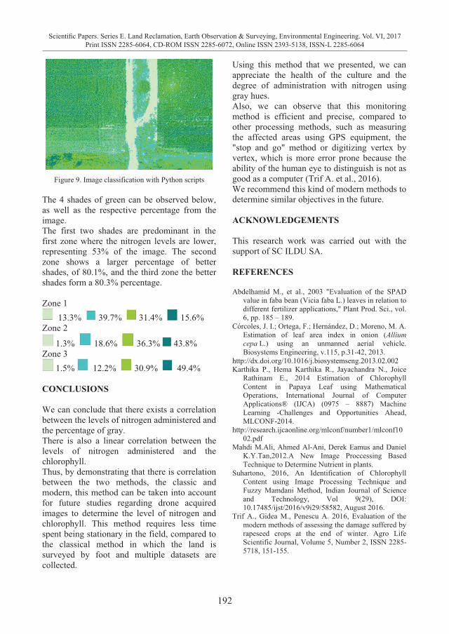
192
Scientific Papers. Series E. Land Reclamation, Earth Observation & Surveying, Environmental Engineering. Vol. VI, 2017Print ISSN 2285-6064, CD-ROM ISSN 2285-6072, Online ISSN 2393-5138, ISSN-L 2285-6064
Figure 9. Image classification with Python scripts
The 4 shades of green can be observed below, as well as the respective percentage from the image. The first two shades are predominant in the first zone where the nitrogen levels are lower, representing 53% of the image. The second zone shows a larger percentage of better shades, of 80.1%, and the third zone the better shades form a 80.3% percentage. Zone 1
13.3% 39.7% 31.4% 15.6% Zone 2
1.3% 18.6% 36.3% 43.8% Zone 3
1.5% 12.2% 30.9% 49.4% CONCLUSIONS We can conclude that there exists a correlation between the levels of nitrogen administered and the percentage of gray. There is also a linear correlation between the levels of nitrogen administered and the chlorophyll. Thus, by demonstrating that there is correlation between the two methods, the classic and modern, this method can be taken into account for future studies regarding drone acquired images to determine the level of nitrogen and chlorophyll. This method requires less time spent being stationary in the field, compared to the classical method in which the land is surveyed by foot and multiple datasets are collected.
Using this method that we presented, we can appreciate the health of the culture and the degree of administration with nitrogen using gray hues. Also, we can observe that this monitoring method is efficient and precise, compared to other processing methods, such as measuring the affected areas using GPS equipment, the "stop and go" method or digitizing vertex by vertex, which is more error prone because the ability of the human eye to distinguish is not as good as a computer (Trif A. et al., 2016). We recommend this kind of modern methods to determine similar objectives in the future. ACKNOWLEDGEMENTS This research work was carried out with the support of SC ILDU SA. REFERENCES
Abdelhamid M., et al., 2003 "Evaluation of the SPAD
value in faba bean (Vicia faba L.) leaves in relation to different fertilizer applications," Plant Prod. Sci., vol. 6, pp. 185 – 189.
Córcoles, J. I.; Ortega, F.; Hernández, D.; Moreno, M. A. Estimation of leaf area index in onion (Allium cepa L.) using an unmanned aerial vehicle. Biosystems Engineering, v.115, p.31-42, 2013.
http://dx.doi.org/10.1016/j.biosystemseng.2013.02.002 Karthika P., Hema Karthika R., Jayachandra N., Joice
Rathinam E., 2014 Estimation of Chlorophyll Content in Papaya Leaf using Mathematical Operations, International Journal of Computer Applications® (IJCA) (0975 – 8887) Machine Learning -Challenges and Opportunities Ahead, MLCONF-2014.
http://research.ijcaonline.org/mlconf/number1/mlconf1002.pdf
Mahdi M.Ali, Ahmed Al-Ani, Derek Eamus and Daniel K.Y.Tan,2012.A New Image Proccessing Based Technique to Determine Nutrient in plants.
Suhartono, 2016, An Identification of Chlorophyll Content using Image Processing Technique and Fuzzy Mamdani Method, Indian Journal of Science and Technology, Vol 9(29), DOI: 10.17485/ijst/2016/v9i29/58582, August 2016.
Trif A., Gidea M., Penescu A. 2016, Evaluation of the modern methods of assessing the damage suffered by rapeseed crops at the end of winter. Agro Life Scientific Journal, Volume 5, Number 2, ISSN 2285-5718, 151-155.