Journal of Computational and Applied Mathematics 178 (2005) 191–203

www.elsevier.com/locate/cam

Weak classical orthogonal polynomials in two variables�

Lidia Fernándeza, Teresa E. Pérezb,∗, Miguel A. PiñarbaDepartamento de Matemática Aplicada, Universidad de Granada, 18071 Granada, Spain

bDepartamento de Matemática Aplicada and Instituto Carlos I de Física Teórica y Computacional,Universidad de Granada, 18071 Granada, Spain

Received 2 October 2003; received in revised form 16 February 2004

Abstract

Orthogonal polynomials in two variables constitute a very old subject in approximation theory. Usually they arestudied as solutions of second-order partial differential equations. In this work, we study two-variable orthogonalpolynomials associated with a moment functional satisfying the two-variable analogue of the Pearson differentialequation. From this approach, we derive the extension of some of the usual characterizations of the classicalorthogonal polynomials in one variable.© 2004 Elsevier B.V. All rights reserved.

MSC:33C50

Keywords:Orthogonal polynomials in two variables; Classical orthogonal polynomials

1. Introduction

One of the most important characterizations of the classical orthogonal polynomials in one variablewas given by Bochner in 1929 (see[1]). Let {Pn}n be a sequence of classical orthogonal polynomials(Hermite, Laguerre, Jacobi or Bessel), thenPn(x) is solution of the second-order differential equation

�(x)y′′ + �(x)y′ = �ny, (1)

� Partially supported by Ministerio de Ciencia y Tecnología (MCYT) of Spain and by the European Regional DevelopmentFund (ERDF) through the grant BFM2001-3878-C02-02, Junta de Andalucía, G.I. FQM 0229 and INTAS Project 2000-272.∗ Corresponding author.

E-mail address:tperez@ugr.es(T.E. Pérez).

0377-0427/$ - see front matter © 2004 Elsevier B.V. All rights reserved.doi:10.1016/j.cam.2004.08.010

192 L. Fernández et al. / Journal of Computational and Applied Mathematics 178 (2005) 191–203

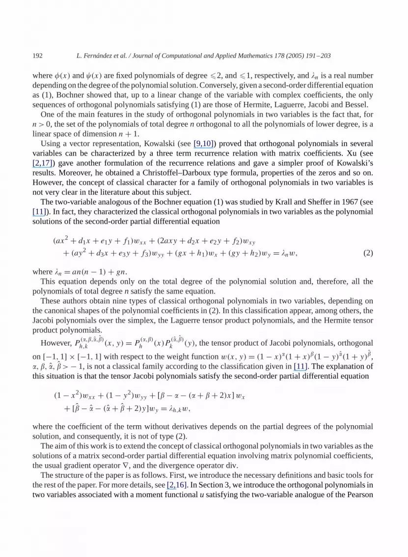
where�(x) and�(x) are fixed polynomials of degree�2, and�1, respectively, and�n is a real numberdependingon thedegreeof thepolynomial solution.Conversely, givenasecond-order differential equationas (1), Bochner showed that, up to a linear change of the variable with complex coefficients, the onlysequences of orthogonal polynomials satisfying (1) are those of Hermite, Laguerre, Jacobi and Bessel.One of the main features in the study of orthogonal polynomials in two variables is the fact that, for

n>0, the set of the polynomials of total degreen orthogonal to all the polynomials of lower degree, is alinear space of dimensionn+ 1.Using a vector representation, Kowalski (see[9,10]) proved that orthogonal polynomials in several

variables can be characterized by a three term recurrence relation with matrix coefficients. Xu (see[2,17]) gave another formulation of the recurrence relations and gave a simpler proof of Kowalski’sresults. Moreover, he obtained a Christoffel–Darboux type formula, properties of the zeros and so on.However, the concept of classical character for a family of orthogonal polynomials in two variables isnot very clear in the literature about this subject.The two-variable analogous of the Bochner equation (1) was studied by Krall and Sheffer in 1967 (see

[11]). In fact, they characterized the classical orthogonal polynomials in two variables as the polynomialsolutions of the second-order partial differential equation

(ax2 + d1x + e1y + f1)wxx + (2axy + d2x + e2y + f2)wxy+ (ay2 + d3x + e3y + f3)wyy + (gx + h1)wx + (gy + h2)wy = �nw, (2)

where�n = an(n− 1)+ gn.This equation depends only on the total degree of the polynomial solution and, therefore, all the

polynomials of total degreen satisfy the same equation.These authors obtain nine types of classical orthogonal polynomials in two variables, depending on

the canonical shapes of the polynomial coefficients in (2). In this classification appear, among others, theJacobi polynomials over the simplex, the Laguerre tensor product polynomials, and the Hermite tensorproduct polynomials.

However,P (�,�,�,�)h,k (x, y)= P (�,�)h (x)P(�,�)k (y), the tensor product of Jacobi polynomials, orthogonal

on [−1,1] × [−1,1] with respect to the weight functionw(x, y)= (1− x)�(1+ x)�(1− y)�(1+ y)�,�, �, �, �>− 1, is not a classical family according to the classification given in[11]. The explanation ofthis situation is that the tensor Jacobi polynomials satisfy the second-order partial differential equation

(1− x2)wxx + (1− y2)wyy + [� − � − (� + � + 2)x] wx

+ [� − � − (� + � + 2)y]wy = �h,kw,

where the coefficient of the term without derivatives depends on the partial degrees of the polynomialsolution, and consequently, it is not of type (2).The aim of this work is to extend the concept of classical orthogonal polynomials in two variables as the

solutions of a matrix second-order partial differential equation involving matrix polynomial coefficients,the usual gradient operator∇, and the divergence operator div.The structure of the paper is as follows. First, we introduce the necessary definitions and basic tools for

the rest of the paper. Formore details, see[2,16]. In Section 3, we introduce the orthogonal polynomials intwo variables associated with a moment functionalu satisfying the two-variable analogue of the Pearson

L. Fernández et al. / Journal of Computational and Applied Mathematics 178 (2005) 191–203 193

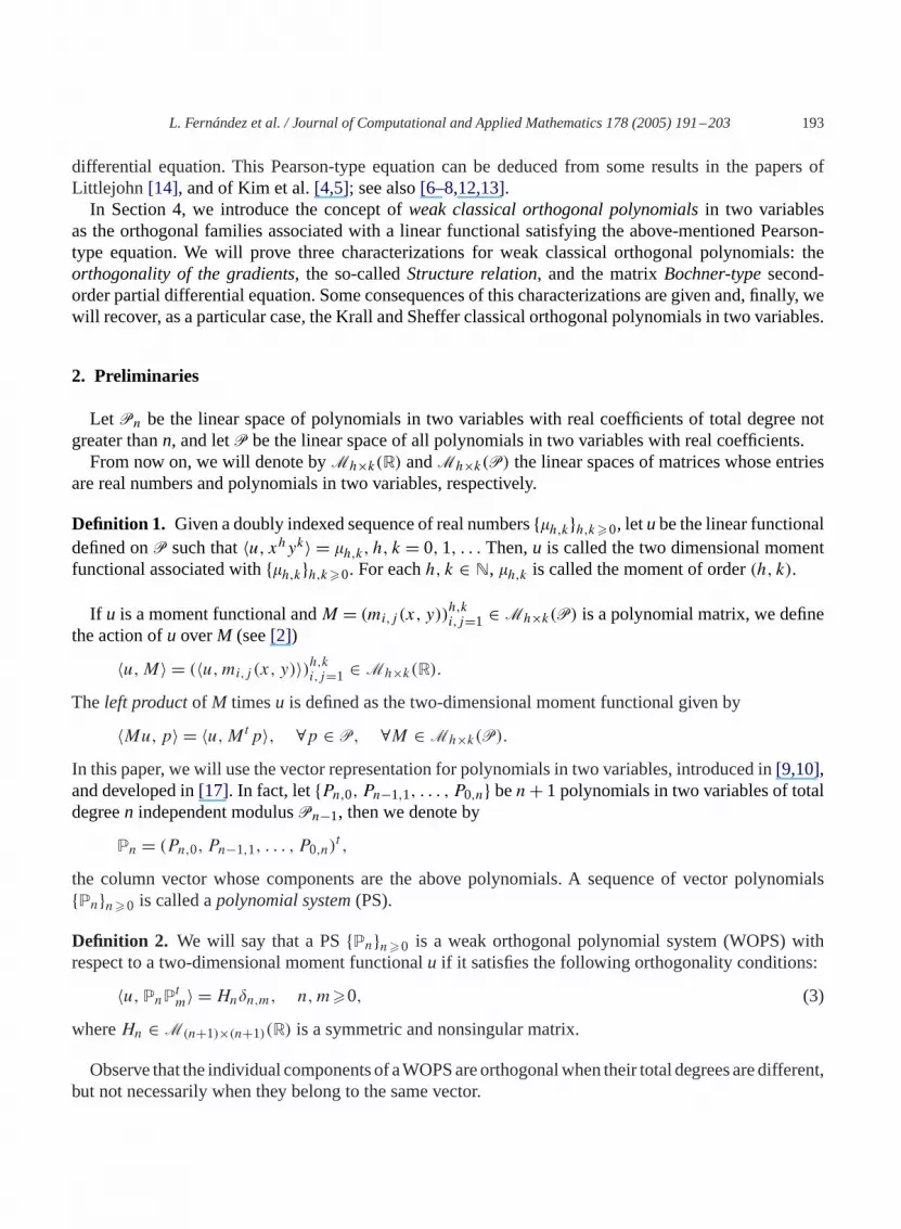
differential equation. This Pearson-type equation can be deduced from some results in the papers ofLittlejohn [14], and of Kim et al.[4,5]; see also[6–8,12,13].In Section 4, we introduce the concept ofweak classical orthogonal polynomialsin two variables

as the orthogonal families associated with a linear functional satisfying the above-mentioned Pearson-type equation. We will prove three characterizations for weak classical orthogonal polynomials: theorthogonality of the gradients, the so-calledStructure relation, and the matrixBochner-typesecond-order partial differential equation. Some consequences of this characterizations are given and, finally, wewill recover, as a particular case, the Krall and Sheffer classical orthogonal polynomials in two variables.

2. Preliminaries

Let Pn be the linear space of polynomials in two variables with real coefficients of total degree notgreater thann, and letP be the linear space of all polynomials in two variables with real coefficients.From now on, we will denote byMh×k(R) andMh×k(P) the linear spaces of matrices whose entries

are real numbers and polynomials in two variables, respectively.

Definition 1. Given a doubly indexed sequence of real numbers{�h,k}h,k�0, letube the linear functionaldefined onP such that〈u, xhyk〉 = �h,k, h, k = 0,1, . . . Then,u is called the two dimensional momentfunctional associated with{�h,k}h,k�0. For eachh, k ∈ N, �h,k is called the moment of order(h, k).

If u is a moment functional andM = (mi,j (x, y))h,ki,j=1 ∈ Mh×k(P) is a polynomial matrix, we definethe action ofu overM (see[2])

〈u,M〉 = (〈u,mi,j (x, y)〉)h,ki,j=1 ∈ Mh×k(R).

The left productofM timesu is defined as the two-dimensional moment functional given by

〈Mu,p〉 = 〈u,Mtp〉, ∀p ∈ P, ∀M ∈ Mh×k(P).

In this paper, we will use the vector representation for polynomials in two variables, introduced in[9,10],and developed in[17]. In fact, let{Pn,0, Pn−1,1, . . . , P0,n} ben+ 1 polynomials in two variables of totaldegreen independent modulusPn−1, then we denote by

Pn = (Pn,0, Pn−1,1, . . . , P0,n)t ,the column vector whose components are the above polynomials. A sequence of vector polynomials{Pn}n�0 is called apolynomial system(PS).

Definition 2. We will say that a PS{Pn}n�0 is a weak orthogonal polynomial system (WOPS) withrespect to a two-dimensional moment functionalu if it satisfies the following orthogonality conditions:

〈u,PnPtm〉 =Hn�n,m, n,m�0, (3)

whereHn ∈ M(n+1)×(n+1)(R) is a symmetric and nonsingular matrix.

Observe that the individual componentsof aWOPSareorthogonalwhen their total degreesaredifferent,but not necessarily when they belong to the same vector.

194 L. Fernández et al. / Journal of Computational and Applied Mathematics 178 (2005) 191–203

If Hn is a diagonal matrix then we say that the WOPS{Pn}n�0 is anorthogonal polynomial system(OPS). In the particular case whereHn is the identity matrix, we call{Pn}n�0 anorthonormal polynomialsystem.Moreover, a WOPS is called amonomialWOPS if every polynomial contains only a higher degree

term, that is,

Ph,k(x, y)= ch,kxhyk + R(x, y), h+ k = n,with ch,k �= 0 a real constant andR(x, y) ∈ Pn−1. If ch,k = 1 then we will say that{Pn}n�0 is amonicWOPS.As usual, we say that a two-dimensional moment functionalu is quasi-definiteif there exists an OPS

or, equivalently, if there exists an unique monic WOPS relative tou.Now, we recall the definitions of thegradient (∇), and thedivergence(div) operators acting over

polynomials in two variables

∇p =(

�xp�yp

), div

(p

q

)= �xp + �yq, ∀p, q ∈ P.

Moreover,wedefine thedistributional gradient operatorand thedistributional divergenceoperatoractingover two-dimensional moment functionals in the following way:⟨

∇u,(p

q

)⟩= −

⟨u,div

(p

q

)⟩= −〈u, �xp + �yq〉, ∀p, q ∈ P,

⟨div

(u1u2

), p

⟩= −

⟨(u1u2

),∇p

⟩= −(〈u1, �xp〉 + 〈u2, �yp〉), ∀p ∈ P.

Wecan extend, in a natural way, the action of∇ and div over a two-variable polynomialmatrix, as follows:Definition 3. LetM,N ∈ Mh×k(P) be polynomial matrices. We define

∇M =(

�xM�yM

)∈ M2h×k(P), div

(M

N

)= �xM + �yN ∈ Mh×k(P).

3. Pearson two-dimensional moment functionals

In this section, we define the concept ofPearsontwo-dimensional moment functional as the linearfunctional satisfying a Pearson-type equation in the following way.

Definition 4. A moment functionalu is said to bePearsonif it satisfies the Pearson-type equation

div(�u)= �tu, (4)

that is,〈div(�u), p〉 = 〈�tu, p〉,∀p ∈ P, where

� =(a b

b c

), � =

(d

e

), (5)

L. Fernández et al. / Journal of Computational and Applied Mathematics 178 (2005) 191–203 195

are polynomial matrices such thata=a(x, y), b=b(x, y), andc=c(x, y) are polynomials of total degree�2, d = d(x, y), e = e(x, y) are polynomials of total degree�1, and det〈u,�〉 �= 0.

Using the distributional operations defined in the previous section, this definition means

−〈u, a�xp + b�yp〉 = 〈u, dp〉,−〈u, b�xp + c�yp〉 = 〈u, ep〉, ∀p ∈ P.

This kind of relation, written in a different way, can be found in the paper of Littlejohn[14], and in thepapers of Kim et al.[4,5].In this moment, we need to define the left multiplication of�∇ and� times a polynomial matrix.

Definition 5. LetM ∈ Mh×k(P), and�, � as given in (5). We define

�∇M =(a�xM + b�yMb�xM + c�yM

)∈ M2h×k(P), �M =

(dM

eM

)∈ M2h×k(P),

�t∇M = d�xM + e�yM ∈ Mh×k(P).

Observe that in the above definition�M is the standard Kronecker product of matrices (see[3, p. 242]).In fact all the previous definitions are inspired in the Kronecker product.From the above definitions, it is easy to prove the following:

Lemma 6. LetM ∈ Mh×k(P) andN ∈ Mk×m(P) be two polynomial matrices. Then, we have

(i) �∇(MN)= (�∇M)N + diag(M,M)(�∇N) ∈ M2h×m(P),(ii) �(MN)= (�M)N ∈ M2h×m(P),(iii) div (diag(M,M)�∇N)=Mdiv(�∇N)+(∇Mt)t�∇N ∈ M2h×m(P),where,as usual, diag(M,M)

denotes the diagonal block matrix

diag(M,M)=(M 00 M

)∈ M2h×2k(P).

Observe that, ifu is a Pearson moment functional, then we can write (4) as follows:

�∇u= �u, where� = � − (div�)t =(d − ax − bye − bx − cy

). (6)

From (6), we deduce that ifu is a two-dimensional weak classical moment functional, then

div(�∇u)− div(�u)= 0. (7)

Denote by

a(x, y)= a20x2 + a11xy + a02y2 + a10x + a01y + a0,b(x, y)= b20x2 + b11xy + b02y2 + b10x + b01y + b0,c(x, y)= c20x2 + c11xy + c02y2 + c10x + c01y + c0,d(x, y)= d10x + d01y + d0,e(x, y)= e10x + e01y + e0,

196 L. Fernández et al. / Journal of Computational and Applied Mathematics 178 (2005) 191–203

the explicit expressions of the polynomials involved in (5), and let us denote by{Pn}n amonic polynomialsystem. From the above definition, we deduce that

〈div(�u),Pn〉 = 〈�tu,Pn〉, n�0, (8)

that is,〈u,�∇Pn + �Pn〉 = 0, n�0. Using Definition 5,�∇Pn + �Pn is a 2(n + 1) × 1 polynomialmatrix of degree less than or equal ton+ 1. Then, we can write

�∇Pn + �Pn = �n+1Pn+1 +n∑m=0

Cn,mPm, Cn,m ∈ M2(n+1)×(m+1)(R), (9)

where

�n+1 =(

�1n+1�2n+1

)∈ M2(n+1)×(n+2)(R), (10)

is defined from the four-diagonal matrices

�mn+1 = (wmi,j )(n+1)×(n+2)i,j=1 , m= 1,2,

as follows:

w1i,i−1 = (i − 1)b20,

w1i,i = (n+ 1− i)a20+ (i − 1)b11+ d10,w1i,i+1 = (n+ 1− i)a11+ (i − 1)b02+ d01,w1i,i+2 = (n+ 1− i)a02,

and

w2i,i−1 = (i − 1)c20,

w2i,i = (n+ 1− i)b20+ (i − 1)c11+ e10,w1i,i+1 = (n+ 1− i)b11+ (i − 1)c02+ e01,w1i,i+2 = (n+ 1− i)b02,

for 1�i�n+ 1, andw1i,j = w2i,j = 0, otherwise.In the same way, using (7), we have

〈u,div(�∇Ptn)+ �t∇Ptn〉 = 0, n�0,

where div(�∇Ptn)+ �t∇Ptn is a 1× (n+1) polynomial matrix of degree less than or equal ton, and then

div(�∇Ptn)+ �t∇Ptn = Ptnn +

n−1∑m=0

PtmDn,m,

L. Fernández et al. / Journal of Computational and Applied Mathematics 178 (2005) 191–203 197

whereDn,m ∈ M(m+1)×(n+1)(R), andn ∈ M(n+1)×(n+1)(R) is given by

tn = J (n)�n, J (n)=

n 0 ... 00 n− 1 ... 0

. . .

0 0 ... 10 0 ... 0

0 ... 0 01 ... 0 0. . .

0 ... n− 1 00 ... 0 n

. (11)

4. Weak classical orthogonal polynomials

In this section, we introduce the concept of two-dimensional weak classical moment functional froma Pearson-type differential equation satisfied by a linear functionalu, as Marcellán, Branquinho, andPetronilho did in[15].

Definition 7. We will say that a two-dimensional moment functionalu is weak classical if it is quasi-definite, Pearson,

rank�1n+1 = rank�2n+1 = n+ 1, n�0, (12)

rank�n+1 = n+ 2, n�0, (13)

andn is a nonsingular matrix.

We must remark that the rank condition for�n (13) can be deduced from the nonsingular character ofn, because

n+ 1= rank(n)= rank(J (n)�n)�rank(�n).

A WOPS with respect tou is called aweak classical OPS. From now on, we will denote by{Pn}n themonic weak classical OPS with respect tou.Using the weak classical character ofu, some interesting properties can be deduced. Forn = 0, then

P0 = 1, and we have

0= 〈�tu,P0〉 = 〈u,�〉,that is,〈u, d〉=0, and〈u, e〉=0. From the quasi-definite character ofu, we deduce that degd=dege=1.Forn= 1, we have∇Pt1 = I2, whereI2 denotes the identity matrix of order two, and then

−〈u,�〉 = 〈div(�u),Pt1〉 = 〈�tu,Pt1〉 = 〈u,�Pt1〉.This expression gives

〈u, a + xd〉 = 〈u, c + ye〉 = 0, 〈u, yd〉 = 〈u, xe〉.Now, we have the necessary tools in order to prove the first characterization of weak classical orthogonalpolynomials in two variables.

198 L. Fernández et al. / Journal of Computational and Applied Mathematics 178 (2005) 191–203

Proposition 8 (Orthogonality of the gradients). Let {Pn}n�0 be the monic WOPS with respect to atwo-dimensional moment functional u. Then u is weak classical if and only if{∇Ptn}n�1 satisfy theorthogonality relations

〈u, (∇Ptm)t�∇Ptn〉 = Hn�n,m, n,m�1, (14)

whereHn ∈ M(n+1)×(n+1)(R) is a symmetric and nonsingular matrix.

Proof. Form�1,∇Ptm is a polynomial matrix of dimension 2× (m+ 1) whose entries are polynomialsof degree less than or equal tom− 1. Then,

∇Ptm =m−1∑j=0

diag(Ptj ,Ptj )

(E1m,j

E2m,j

)=m−1∑j=0

diag(Ptj ,Ptj )Em,j ,

whereEm,j ∈ M2(j+1)×(m+1)(R), andEm,m−1 = J (m)t ∈ M2m×(m+1)(R).On the other hand, using Lemma 6, and (4), we get

〈u,diag(Pj ,Pj )�∇Ptn〉 = 〈u,�∇(PjPtn)〉 − 〈u, (�∇Pj )Ptn〉

= − 〈div(�u),PjPtn〉 − 〈u, (�∇Pj )Ptn〉

= − 〈�tu,PjPtn〉 − 〈u, (�∇Pj )Ptn〉

= − 〈u, (�Pj + �∇Pj )Ptn〉,

and then,〈u, (∇Ptm)t�∇Ptn〉 = −∑m−1

j=0Etm,j[〈u, (�Pj + �∇Pj )P

tn〉]. Using (9) and (11), we obtain

〈u, (∇Ptm)t�∇Ptn〉 = −J (n)�nHn�n,m = −tnHn�n,m.

Conversely, let us assume that{Pn}n�0 satisfy the orthogonality conditions (14). We want to prove thatu is weak classical, that is, there exists a 2× 1 vector matrix� of exact degree 1 whose components areindependent moduloP0 such that div(�u)= �tu, that is,

〈div(�u),Ptn〉 = 〈�tu,Ptn〉, n�0.

Forn= 1, notice that∇Pt1 = I2. Thus,〈div(�u),Pt1〉 = −〈u,�∇Pt1〉 = −〈u, (∇Pt1)

t�∇Pt1〉 = −H1,whereH1 ∈ M2×2(R) is a nonsingular matrix. In this way, we define the 2× 1 polynomial vector� = −H1H−1

1 P1, because it satisfies

〈�tu,P1〉 = −〈Pt1H−11 H1u,Pt1〉 = −H1.

Moreover, forn�2, we get

〈div(�u),Ptn〉 = −〈u,�∇Ptn〉 = −〈u, (∇Pt1)t�∇Ptn〉 = 0.

On the other hand, using the orthogonality condition, we have

〈�tu,Ptn〉 = 〈u,�Ptn〉 = −H1H−11 〈u,P1P

tn〉 = 0, n�2.

L. Fernández et al. / Journal of Computational and Applied Mathematics 178 (2005) 191–203 199

Finally, observe that this relation holds forn= 0 taking into account that

〈div(�u),Pt0〉 = 0. �

The second characterization that we will show is the so-calledStructure relation. This relation appearsin another form in[4,5].

Proposition 9 (The structure relation). Let u be a quasi-definite moment functional and{Pn}n�0 themonic WOPS with respect to u. Then u is weak classical if and only if{Pn}n�0 satisfies

�∇Ptn = diag(Ptn+1,Ptn+1)F nn+1 + diag(Ptn,Ptn)Fnn + diag(Ptn−1,Ptn−1)F nn−1,

for n�1,where

Fnm =(Fnm,1

Fnm,2

)∈ M2(m+1)×(n+1)(R),

such that

rankFnn−1,i = n, i = 1,2, rankFnn−1 = n+ 1, n�1.

Proof. Suppose thatu is weak classical, that is,u satisfies the Pearson-type equation (4). Using ananalogous reasoning as in the above Proposition,�∇Ptn is a 2× (n + 1) matrix with two-variablepolynomial entries of degree at mostn+ 1. Then, we can express

�∇Ptn =n+1∑m=0

diag(Ptm,Ptm)

(Fnm,1

Fnm,2

)=n+1∑m=0

diag(Ptm,Ptm)Fnm,

whereFnm can be obtained as follows:

diag(Hm,Hm)Fnm = 〈u,diag(Pm,Pm)(�∇Ptn)〉 = −〈u, (�Pm + �∇Pm)P

tn〉,

and, from the orthogonality, we deduceFnm = 0, form<n− 1. Moreover, using (9), we get

diag(Hn−1, Hn−1)F nn−1 = −〈u, (�Pn−1 + �∇Pn−1)Ptn〉 = −�nHn.

Obviously, the rank conditions will be deduced from the above relation.In order to prove the converse result, we calculate

〈div(�u),Ptn〉= −〈u,�∇Ptn〉 = −〈u,diag(Ptn+1,Ptn+1)〉Fnn+1−〈u,diag(Ptn,Ptn)〉Fnn − 〈u,diag(Ptn−1,Ptn−1)〉Fnn−1,

and then〈div(�u),Ptn〉 = 0, for n�2, and trivially, forn= 0. Forn= 1, using the structure relation, weget

〈div(�u),Pt1〉 = −〈u,�∇Pt1〉 = −diag(H0, H0)F 10 .Finally, if we define�t=−Pt1H

−11 (F 10 )

tdiag(H0, H0), from the nonsingular character of thematricesH1,F 10 and diag(H0, H0), then we deduce that� is a vector polynomial of exact degree 1 whose componentsare independent.�

200 L. Fernández et al. / Journal of Computational and Applied Mathematics 178 (2005) 191–203

Using the corresponding change of basis, we can easily deduce that the structure relation holds forevery WOPS, associated with a weak classical moment functional.

Corollary 10. Let {Qn}n�0 be a WOPS associated with a moment functional u, and letQtn = PtnAn,n�0,be the corresponding change of basis. Then u is weak classical if and only if forn�1

�∇Qtn = diag(Qtn+1,Qtn+1)F nn+1 + diag(Qtn,Qtn)Fnn + diag(Qtn−1,Qtn−1)F nn−1,

whereF nm = diag(A−1m ,A

−1m )F

nmA

tn.

The last characterization constitutes the natural generalization of the Bochner differential equation forone-variable classical orthogonal polynomials.Let us define the differential operator

L[p] = div(�∇p)+ �t∇p, p ∈ P,

where� is a symmetric (2× 2) two-variable polynomial matrix like in (5) and� = (d, e)t is a vectorpolynomial of degree less than or equal to 1. Observe that theformal Lagrange adjointof L is given by(7),

L∗[u] = div(�∇u)− div(�u),

since it satisfies

〈L∗[u], p〉 = 〈u,L[p]〉, p ∈ P.

Using the explicit expression of� and�, we obtain

L[p] = a�xxp + 2b�xyp + c�yyp + d�xp + e�yp,whered = d + ax + by ande = e + bx + cy , with deg(L[p])� deg(p).Observe thatL[p] is the natural generalization of the left-hand side of the Krall and Sheffer partial

differential equation (2) without restrictions in the coefficients. Using Definition 5, the operatorL can beapplied to a polynomial matrix as follows:

L[M] = div(�∇M)+ �t∇M.

In this way, we can easily deduce

Lemma 11. Let u be a quasi-definite moment functional, and{Pn}n�0 the corresponding monicWOPS.If there exists a sequence{n}n�1, of nonsingular matricesn ∈ M(n+1)×(n+1)(R), such that

L[Ptn] = Ptnn, n�1, (15)

thenL∗[u] = 0.

And, from Lemma 6, we can prove the following:

Lemma 12. Let {Pn}n�0 be a PS. Then,

L[PnPtm] = L[Pn] Ptm + PnL[Ptm] + 2(∇Ptn)t�∇Ptm.

L. Fernández et al. / Journal of Computational and Applied Mathematics 178 (2005) 191–203 201

Now, we have the necessary tools in order to prove the

Proposition 13 (Matrix partial differential equation). Let u be a quasi-definite moment functional and{Pn}n�0 the corresponding monic WOPS. Then u is weak classical if and only if there exists a sequence{n}n�1, of nonsingular matricesn ∈ M(n+1)×(n+1)(R) such that

L[Ptn] ≡ div(�∇Ptn)+ �t∇Ptn = Ptnn, (16)

〈u, yd〉 = 〈u, xe〉. (17)

Proof. Let u be a weak classical moment functional, thenL∗[u] = 0. Using Lemma 12 we get

0= 〈L∗[u],PmPtn〉 = 〈u,L[PmPtn]〉= 〈u,L[Pm]Ptn〉 + 〈u,Pm L[Ptn]〉 + 2〈u, (∇Ptm)

t�∇Ptn〉.From Proposition 8, we get〈u, (∇Ptm)

t�∇Ptn〉 = 0, for m<n, and from the orthogonality condition,〈u,L[Pm]Ptn〉 = 0, form<n. Therefore,

〈u,Pm L[Ptn]〉 = 0, m<n,

that is, the 1× (n+1) vector polynomial of degree at mostn,L[Ptn], is orthogonal toPm form<n. ThenL[Ptn] = Ptnn,

wheren is given by (11).The proof of the converse is analogous to the above characterizations. If we assume that{Pn}n�0

satisfies (16), then, from Lemma 11, we getL∗[u] = 0, and therefore

0= 〈L∗[u],Pt1〉 = 〈u,L[Pt1]〉 = 〈u,div(�∇Pt1)+ �t∇Pt1〉 = 〈u,div� + �

t 〉,that is, 〈u,�t 〉 = 0, where�t = div� + �

t = (d, e). From the quasi-definite character ofu, we getdegd = dege = 1, and therefore they are orthogonal toP0. Using Lemma 12, we get

0= 〈L∗[u],P1Ptn〉 = 〈u,L[P1]Ptn〉 + 〈u,P1L[Ptn]〉 + 2〈u, (∇Pt1)

t�∇Ptn〉,and then〈div(�u),Ptn〉 = −〈u,�∇Ptn〉 = 0, for n�0 andn = 0. Moreover, in this case,〈�tu,Ptn〉 =〈u,�Ptn〉 = 0. Forn= 1, we need to prove〈div(�u),Pt1〉 = 〈�tu,Pt1〉, or equivalently

〈u,�∇Pt1 + �Pt1〉 = 〈u,� + �Pt1〉 =( 〈u, a + xd〉 〈u, b + yd〉

〈u, b + xe〉 〈u, c + ye〉)

= 0.

Observe that

0= 〈L∗[u], x2〉 = 〈u,L[x2]〉 = 2〈u, a + xd〉,0= 〈L∗[u], y2〉 = 〈u,L[y2]〉 = 2〈u, c + ye〉,0= 〈L∗[u], xy〉 = 〈u,L[xy]〉 = 〈u,2b + yd + xe〉.

Finally, using (17) the result follows.�

202 L. Fernández et al. / Journal of Computational and Applied Mathematics 178 (2005) 191–203

Thematrix partial differential equation (16) is satisfied by everyWOPSassociatedwith aweak classicalmoment functionalu. Using the corresponding change of basis, we can deduce

Corollary 14. Let {Qn}n aWOPS associated with a weak classical moment functional u, and letAn thenonsingular matrix corresponding to the change of basisQtn = PtnAn, n�0.Then,

L[Qtn] = Qtnn,

wheren = A−1n nAn, that is, n andn are similar matrices.

Taking into consideration the above corollary, the point now is to obtain necessary and sufficientconditions to guarantee the diagonal character of the matricesn for a given orthogonal polynomialsequence. If this is the case, then every polynomial in the sequence satisfies a holonomic second-orderpartial differential equation.

Proposition 15. Let u be a weak classical moment functional, and let{Pn}n�0 be the correspondingmonic WOPS. Then, the following statements are equivalent

(i) the matrixn is diagonal, ∀n�1,(ii) the polynomials a, b, c, d, and e in(5) are monomial, that is, they verify

a11= a02= b20= b02= c20= c11= d01= e10= 0. (18)

Proof. Let us assume that the matrixn in Eq. (16) is diagonal, with

n = diag(�n,0, �n−1,1, . . . , �0,n).

Then, every polynomialPh,k, with h+ k = n, satisfies the partial differential equationa�xxPh,k + 2b�xyPh,k + c�yyPh,k + d�xPh,k + e�yPh,k = �h,kPh,k. (19)

The explicit expressions fora, b, c, d, ande follow by substitution of the orthogonal polynomials of totaldegree one and two.Conversely, if we assume that the coefficients in the second-order partial differential equation have the

form (18), then the coefficient of the highest degree term in (19) is

a20k(k − 1)+ 2b11hk + c02h(h− 1)+ d10k + e01h,which is different from zero as we can check from the quasi-definite character of the moment functional.Therefore,L[Ph,k] is a monic polynomial of total degreen, which is orthogonal to every polynomial oflower degree. In this way,

L[Ph,k] ≡ div(�∇Ph,k)+ �t∇Ph,k = �h,kPh,k, h+ k = n, n�0. �

Remark. Finally, wemust remark that, ifn is an scalar matrix for every value ofn, that is,n=�nIn+1,where�n is a real number andIn+1 is the identitymatrix of ordern+1, then all the orthogonal polynomialsof total degreen satisfy the same second-order partial differential equation (given by (2)), and we recoverthe classical orthogonal polynomials in two variables deduced in[11].

L. Fernández et al. / Journal of Computational and Applied Mathematics 178 (2005) 191–203 203

Acknowledgements

The authors thank the referee for their valuable comments about the content and some references whichwe had not considered in our first version of the manuscript.

References

[1] S. Bochner, Über Sturm-Liouvillesche Polynomsysteme, Math. Zeit. 29 (1929) 730–736.[2] C.F. Dunkl, Y. Xu, Orthogonal polynomials of several variables, Encyclopedia of Mathematics and its Applications, vol.

81, Cambridge University Press, Cambridge, 2001.[3] R.A. Horn, C.R. Johnson, Topics in Matrix Analysis, Cambridge University Press, Cambridge, 1991.[4] Y.J. Kim, K.H. Kwon, J.K. Lee, Orthogonal polynomials in two variables and second-order partial differential equations,

J. Comput. Appl. Math. 82 (1997) 239–260.[5] Y.J. Kim, K.H. Kwon, J.K. Lee, Partial differential equations having orthogonal polynomial solutions, J. Comput. Appl.

Math. 99 (1998) 239–253.[6] Y.J. Kim, K.H. Kwon, J.K. Lee, Rodrigues type formula for multi-variate orthogonal polynomials, Bull. Korean Math.

Soc. 38 (2001) 463–474.[7] Y.J. Kim, K.H. Kwon, J.K. Lee, Multi-variate orthogonal polynomials and second-order partial differential equations,

Commun. Appl. Anal. 6 (2002) 479–504.[8] T. Koornwinder, Two-variable analogues of the classical orthogonal polynomials: theory and application of special

functions, Proceedings of Advanced Seminar, Mathematics Research Center, University Wisconsin, Madison, WI, 1975,Publ. No. 35, Academic Press, NewYork, 1975, pp. 435–495.

[9] M.A. Kowalski, The recursion formulas for orthogonal polynomials inn variables, SIAM J. Math. Anal. 13 (1982)309–315.

[10] M.A. Kowalski, Orthogonality and recursion formulas for polynomials inn variables, SIAM J. Math. Anal. 13 (1982)316–323.

[11] H.L. Krall, I.M. Sheffer, Orthogonal polynomials in two variables, Ann. Mat. Pure Appl. Ser. 4 76 (1967) 325–376.[12] K.H. Kwon, J.K. Lee, L.L. Littlejohn, Orthogonal polynomial eigenfunctions of second-order partial differential equations,

Trans. Amer. Math. Soc. 353 (2001) 3629–3647.[13] J.K. Lee, Bivariate version of the Hahn-Sonine theorem, Proc. Amer. Math. Soc. 128 (2000) 2381–2391.[14] L.L. Littlejohn, Orthogonal polynomial solutions to ordinary and partial differential equations, in: M. Alfaro, et al. (Eds.),

Orthogonal Polynomials and their Applications, Proceedings Segovia, Spain, 1986, Lecture Notes in Mathematics, vol.1329, Springer, Berlin, 1988, pp. 98–124.

[15] F. Marcellán, A. Branquinho, J. Petronilho, Classical orthogonal polynomials: a functional approach, ActaAppl. Math. 34(1994) 283–303.

[16] P.K. Suetin, Orthogonal Polynomials in Two Variables, Gordon and Breach, Amsterdam, 1999.[17] Y. Xu, On multivariate orthogonal polynomials, SIAM J. Math. Anal. 24 (1993) 783–794.