Embed Size (px)
Citation preview

Applied Mathematical Sciences, Vol. 7, 2013, no. 7, 315 - 325
Weak Solution of the Singular Cauchy Problem
of Euler-Poisson-Darboux Equation for n = 4
A. Manyonge1, D. Kweyu2, J. Bitok3, H. Nyambane3 and J. Maremwa3
1Department of Pure and Applied Mathematics
Maseno University, Maseno, Kenya
2Department of Mathematics
Kenyatta University, Nairobi, Kenya
3Department of Mathematics and Computer Science
Chepkoilel University College, Eldoret, Kenya
[email protected], [email protected]
Abstract
We consider the singular Cauchy problem of Euler-Poisson-Darbouxequation(EPD) of the form
utt +k
tut = ∇2u
u(x, 0) = f(x), ut(x, 0) = 0
where ∇2 is the Laplacian operator in Rn, n will refer to dimension and
k a real parameter. The EPD equation finds applications in geome-try, applied mathematics, physics etc. Various authors have solved thisproblem for different values of n and k using various techniques sincethe time of Euler[1]. In this paper, we shall take the Fourier transformof the EPD equation with respect to the space coordinate. The equationso obtained is transformed into a Bessel differential equation. We solvethis equation and obtain the inverse Fourier transform of its solution.Finally on using the convolution theorem, we obtain the weak solutionof the EPD equation for n = 4. The case for n = 1 is an interesting onefor this problem as the solution will be that of a 1 − D wave equation.We therefore deduce the weak solution for the 1 − D wave equation aswell.

316 A. Manyonge, D. Kweyu, J. Bitok, H. Nyambane and J. Maremwa
Mathematics Subject Classification: 35Q05
Keywords: Singular Cauchy problem, EPD, Bessel function, weak solu-
tion
1 Introduction
The study of singular Cauchy problems of the Euler-Poisson-Darboux (EPD)
equation is concerned with the equation
utt +k
tut = ∇2u (1)
u(x, 0) = f(x), ut(x, 0) = 0 (2)
where ∇2 is the Laplacian operator in Rn, n will refer to dimension, x =
x1, x2, . . . , xn is a point in Rn, k is a real parameter and t is the time variable.
Problems of type (1) will be called singular if the coefficient kt→ ∞ as t →
0 and degenerate if kt→ 0 as t → 0 in such a way as not to change the
type of problem. In this paper, we shall study singular Cauchy problem of
the EPD type. There has been several approaches by different people to the
question of obtaining the solution of the singular Cauchy problems for the
EPD equation. Our main objective is to obtain a weak solution of the EPD
equation for a general n and deduce solution for n = 4. The case for n = 1
is an interesting one for this problem as the solution will be that of a 1 − D
wave equation. We therefore further deduce the weak solution of the 1 − D
wave equation. The EPD equation for special values of k and n has occurred
in many classical problems in geometry, applied mathematics and physics for
over two centuries. Euler[1] first considered the EPD equation for n = 1.
Using the Riemann method, Martin[2] gave the solution of (1) for n = 1 and
k = −1,−2,−3 . . . . Diaz and Weinberger[3] obtained solutions of ((1) − (2))
for k = n, n+1, n+2 . . . from the known solution for k = n−1. They directly
verified that the resulting formula gives a solution of the problem for any k
with Re(k) > n − 1. Blum[4] obtained solution of the EPD for exceptional
cases k = 1,−3,−5 . . . . Weinstein[5] gave a complete solution of singular
Cauchy problem covering all values of k and n. Blum’s solution differes from
the solution of Weinstein in that the function f is required to have fewer
continuous derivatives i.e. it is sufficient for f to have derivatives of order of
at least (n−k+3)2
. Fusaro[6] solved the boundary value problem of the singular
Cauchy problem of the EPD by separation of variables. Dernek[7], by using a
Weak solution of singular Cauchy problem 317
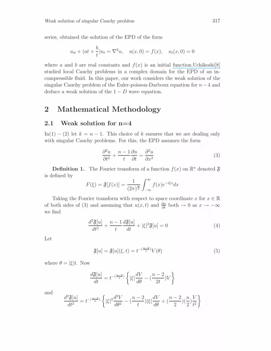
series, obtained the solution of the EPD of the form
utt + (at +b
t)ut = ∇2u, u(x, 0) = f(x), ut(x, 0) = 0
where a and b are real constants and f(x) is an initial function.Uchikoshi[8]
studied local Cauchy problems in a complex domain for the EPD of an in-
compressible fluid. In this paper, our work considers the weak solution of the
singular Cauchy problem of the Euler-poisson-Darboux equation for n−4 and
deduce a weak solution of the 1 − D wave equation.
2 Mathematical Methodology
2.1 Weak solution for n=4
In(1) − (2) let k = n − 1. This choice of k ensures that we are dealing only
with singular Cauchy problems. For this, the EPD assumes the form
∂2u
∂t2+
n − 1
t
∂u
∂t=
∂2u
∂x2(3)
Definition 1. The Fourier transform of a function f(x) on Rn denoted F
is defined by
F (ξ) = F[f(x)] =1
(2π)n2
∫ ∞
−∞f(x)e−iξxdx
Taking the Fourier transform with respect to space coordinate x for x ∈ R
of both sides of (3) and assuming that u(x, t) and ∂u∂t
both → 0 as x → −∞we find
d2F[u]
dt2+
n − 1
t
dF[u]
dt+ |ξ|2F[u] = 0 (4)
Let
F[u] = F[u](ξ, t) = t−(n−2n
)V (θ) (5)
where θ = |ξ|t. Now
dF[u]
dt= t−(n−2
n)
{|ξ|dV
dθ− (
n − 2
2t)V
}
andd2F[u]
dt2= t−(n−2
n)
{|ξ|2d2V
dθ2− (
n − 2
t)|ξ|dV
dθ+ (
n − 2
2)(
n
2)V
t2
}

318 A. Manyonge, D. Kweyu, J. Bitok, H. Nyambane and J. Maremwa
On substitution of the above expressions into (4) we find
|ξ|2d2V
dθ2+
|ξ|t
dV
dθ+
(|ξ|2 − (n − 2)2
4t2
)V = 0
ord2V
dθ2+
1
|ξ|tdV
dθ+
(1 −
(n − 2
2|ξ|t)2)
V = 0
ord2V
dθ2+
1
θ
dV
dθ+
(1 −
(n − 2
2θ
)2)
V = 0
or
d2V
dθ2+
1
θ
dV
dθ+
(1 − (n−2
2)2
θ2
)V = 0 (6)
Equation (6) amounts to a weak formulation of the original EPD, its solution
will therefore be a weak solution. we notice that (6) is Bessel differential
equation of order n−22
whose solution is given by
V (θ) = AJn−22
(θ) + BYn−22
(θ) (7)
where A and B are constants and Jn−22
(θ) and Yn−22
(θ) are Bessel functions
of order n−22
of first and second kind respectively. Now function Yn−22
(θ) is
singular at the origin i.e. Yn−22
(θ) → ∞ as θ → 0. Hence we choose B = 0 so
that
V (|ξ|t) = AJn−22
(|ξ|t) (8)
Now in general, Jn(ξt) is given by
Jn(ξt) =∞∑
r=0
(−1)r
Γ(r + 1)Γ(n + r + 1)
(ξt
2
)2r+n
(9)
from which we find the series expansion of Jn(|ξ|t) as
Jn(|ξ|t) =1
Γ(n + 1)
( |ξ|t2
)n
− 1
Γ(n + 2)
( |ξ|t2
)n+2
+1
2!
1
Γ(n + 3)
( |ξ|t2
)n+4
−. . .
or
Jn−22
(|ξ|t) =1
Γ(n2)
( |ξ|t2
)n−22
− 1
Γ(n+22
)
( |ξ|t2
)n+22
+1
2!
1
Γ(n+42
)
( |ξ|t2
)n+62
− . . .

Weak solution of singular Cauchy problem 319
Thus
F[u] = t−(n−22
)V (θ) = At−(n−22
)
{1
Γ(n2)
( |ξ|t2
)n−22
− 1
Γ(n+22
)
( |ξ|t2
)n+22
+ . . .
}
or
F[u](ξ, t) = A
{1
Γ(n2)
( |ξ|2
)n−22
− 1
Γ(n+22
)
( |ξ|2
)n+22
t2 + . . .
}
Then as t → 0 we have that
F[u](ξ, 0) = A
{1
Γ(n2)
( |ξ|2
)n−22
}= F (|ξ|) by (2)
Thus
A =F (|ξ|)Γ(n
2)(
|ξ|2
)n−22
Hence from (5),
F[u](ξ, t) = t−(n−22
) F (|ξ|)Γ(n2)(
|ξ|2
)n−22
Jn−22
(|ξ|t)
or
F[u](ξ, t) = 2n−2
2 Γ(n
2)F (|ξ|) (|ξ|t)−(n−2
2) Jn−2
2(|ξ|t) (10)
Definition 2. The inverse Fourier transform of F (ξ) in Rn denoted F−1
is defined by
f(x) = F−1[F (ξ)] =1
(2π)n2
∫ ∞
−∞F (ξ)eiξxdξ
The solution of (10) will involve taking the inverse Fourier transform of
both sides and in particular the inverse Fourier transform of the quantity
((|ξ|t)−(n−22
) Jn−22
(|ξ|t)) since for F[f(x)] = F (|ξ|). We state the following the-
orem without proof, for details see [9]
Theorem 3. Bessel function of order n of first kind may be written in
trigonometric form as
(ξt)−n Jn(ξt) =21−n
Γ(n + 12)√
π
∫ π2
0
cos(ξt cos θ) sin2n θdθ

320 A. Manyonge, D. Kweyu, J. Bitok, H. Nyambane and J. Maremwa
Hence from the theorem we have that
(|ξ|t)−(n−22
) Jn−22
(|ξ|t) =2
4−n2
Γ(n−12
)√
π
∫ π2
0
cos(|ξ|t cos θ) sin(n−2) θdθ (11)
In this equation, let z = |ξ|t and
F[Q] = (z)−(n−22
) Jn−22
(z) =2
4−n2
Γ(n−12
)√
π
∫ π2
0
cos(z cos θ) sin(n−2) θdθ (12)
Take the inverse Fourier transform of (12) for x ∈ R on both sides to find
Q(x, t) =1√(2π)
∫ ∞
−∞F[Q]eiξxdξ
or
Q(x, t) =1√(2π)
∫ ∞
−∞
24−n
2
Γ(n−12
)√
π
∫ π2
0
cos(z cos θ) sin(n−2) θeiξxdθdξ
or
Q(x, t) =2−(n−3
2)
Γ(n−12
)π
∫ ∞
−∞
∫ π2
0
cos(z cos θ) sin(n−2) θeiξxdθdξ
or
Q(x, t) =2−(n−3
2)
Γ(n−12
)π
∫ π2
0
∫ ∞
−∞
(ei(z cos θ+ξx) + e−i(z cos θ−ξx)
2
)sin(n−2) θdθdξ
or
Q(x, t) =2−(n−3
2)
Γ(n−12
)π
∫ π2
0
∫ ∞
−∞
(ei(|ξ|t cos θ+xξ) + e−i(|ξ|t cos θ−xξ)
2
)sin(n−2) θdθdξ
Let
E =ei(|ξ|t cos θ+xξ) + e−i(|ξ|t cos θ−xξ)
2(13)
so that
Q(x, t) =2−(n−3
2)
Γ(n−12
)π
∫ π2
0
(∫ 0
−∞Edξ +
∫ ∞
0
Edξ
)sin(n−2) θdθ (14)
or
Q(x, t) =2−(n−1
2)
Γ(n−12
)π
∫ π2
0
(∫ 0
−∞ei(t cos θ+x)ξdξ +
∫ ∞
0
e−i(t cos θ−x)ξdξ
)sin(n−2) θdθ

Weak solution of singular Cauchy problem 321
or
Q(x, t) =2−(n−1
2)
Γ(n−12
)πi
∫ π2
0
(t cos θ
t2 cos2 θ − x2
)sin(n−2) θdθ (15)
We now construct the weak solution of the EPD for n = 4. (15) now becomes
Q(x, t) =2−( 3
2)
Γ(32)πi
∫ π2
0
(t cos θ sin2 θ
t2 cos2 θ − x2
)dθ
or
Q(x, t) =1
232
√π3i
∫ π2
0
(t cos θ sin2 θ
t2 cos2 θ − x2
)dθ (16)
To evaluate the integral in (16) we transform as follows: Let z = eiθ where
0 ≤ θ ≤ 2π. This means that
dθ =dz
iz, sinθ =
(z sin2 −1)2
(2iz)2, cos θ =
zθ2 + 1
2z, cosθ =
(z2 + 1)2
(2z)2
from which we find
t cos θ sin2 θ =t(z2 + 1)(z2 − 1)2
−8z3and t2 cos2 θ − x2 =
t2(z2 + 1)2 − 4x2z2
4z2
inserting these quantities in the integral we find
∫ π2
0
(t cos θ
t2 cos2 θ − x2
)sin2 θdθ = − 1
2it
∫c
(z2 + 1)(z2 − 1)2dz
z2(z4 + (2 − 4x2
t2)z2 + 1)
where c is a unit circle with centre at the origin. The denominator of the right
hand side may be written as
∫ π2
0
(t cos θ
t2 cos2 θ − x2
)sin2 θdθ = − 1
2it
∫c
(z2 + 1)(z2 − 1)2dz
z2(z −√α)(z +
√α)(z −√
β)(z +√
β)
where
√α =
√{(2x2 − t2) + 2x
√x2 − t2
t2
}, −√
α = −√{
(2x2 − t2) + 2x√
x2 − t2
t2
}
√β =
√{(2x2 − t2) − 2x
√x2 − t2
t2
}, −
√β = −
√{(2x2 − t2) − 2x
√x2 − t2
t2
}

322 A. Manyonge, D. Kweyu, J. Bitok, H. Nyambane and J. Maremwa
are the roots of the equation
z4 + (2 − 4x2
t2)z2 + 1
z = 0 obviously lies within c, for the roots√
β and −√β for x > t, it can be
shown that they lie in c. Let
f(z) =(z2 + 1)(z2 − 1)2dz
z2(z4 + (2 − 4x2
t2)z2 + 1)
We examine the residues of f(z) within c. For residue of f(z) at z = 0, this is
a pole of order 2 given by
limz→0
1
1!
d
dz
{(z − 0)2(z2 + 1)(z2 − 1)2
z2(z −√α)(z +
√α)(z −√
β)(z +√
β)
}
With a little simplification, we find
Residue of f(z) at z=0 = −2√
α
α2β(17)
For residue of f(z) at z =√
β we have
limz→√
β
(z2 + 1)(z2 − 1)2
z2(z −√α)(z +
√α)(z +
√β)
=(β + 1)(β − 1)2
2β√
β(β − α)(18)
and for residue of f(z) at z = −√β we have
limz→−√
β
(z2 + 1)(z2 − 1)2
z2(z −√α)(z +
√α)(z −√
β)= −(β + 1)(β − 1)2
2β√
β(β − α)(19)
If ΣR denotes sum of residues of f(z) in c, then from (17), (18) and (19),
ΣR = −2√
α
α2β
and from Cauchy integral theorem
∫ π2
0
(t cos θ
t2 cos2 θ − x2
)sin2 θdθ = − 1
2it2πi(−2
√α
α2β)
or ∫ π2
0
(t cos θ
t2 cos2 θ − x2
)sin2 θdθ =
2π√
α
α2βt

Weak solution of singular Cauchy problem 323
Now our original integral occupied only 14
of c, hence we have∫ π2
0
(t cos θ
t2 cos2 θ − x2
)sin2 θdθ =
2π√
α
α2βt.1
4
or ∫ π2
0
(t cos θ
t2 cos2 θ − x2
)sin2 θdθ =
π
2βtα√
α(20)
Using (20) in (16) we find
Q(x, t) =1
252 iαβt
√α√
π(21)
or
Q(x, t) =1
252 i√
π√
{(2x2 − t2) + 2x√
x2 − t2}(22)
Definition 4. For x ∈ R, let f(x) and g(x) be two given functions. The
convolution of f(x) and g(x) denoted f(x) ∗ g(x) is defined to be the function
(f ∗ g)(x) =
∫�n
f(y)g(x− y)dy
Theorem 5 (Convolution theorem). Let F−1[F1(ξ)] = f(x) and F−1[F2(ξ)] =
g(x), then
F−1[F1(ξ) ∗ F2(ξ)] = f(x) ∗ g(x)
In (10), set n = 4. Taking the inverse Fourier transform of this equation
and using (22), (10) becomes
u(x, t) = 4πf(x) ∗ Q(x, t) (23)
Using the convolution theorem in (23), we find
u(x, t) =1
i
√π
2
∫ ∞
−∞(
f(y)dy√{(2(x − y)2 − t2) + 2(x − y)
√(x − y)2 − t2}
) (24)
2.2 Weak solution for n=1, the case of 1-D wave equa-
tion
Consider (10) when n = 1, i.e.
F[u](x, t) =
√π
2F (|ξ|) (|ξ|t)1
2 J− 12(|ξ|t) (25)

324 A. Manyonge, D. Kweyu, J. Bitok, H. Nyambane and J. Maremwa
and (11) becomes
(|ξ|t) 12 J− 1
2(|ξ|t) =
√2
πcos(|ξ|t) (26)
according to [9]. Using this in (25) we find
F[u](x, t) = F (|ξ|) cos(|ξ|t)
or
u(x, t) =1
i2πf(x) ∗
(t
t2 − x2
)(27)
on use of convolution theorem. Hence
u(x, t) =t
i2π
∫ ∞
−∞
f(y)dy
[t2 − (x − y)2](28)
being the weak solution of the 1 − D wave equation.
3 Conclusion
Equations (24) and (28) obtained represent the weak solutions of the EPD for
n = 4 and n = 1 the 1 − D wave equations respectively.
References
[1] Euler, L.: Foundations of Integral Calculus, vol. 3, Academia Scientiarum
Imperialis Petropolitanae, 1770.
[2] Martin, M.(1951): ’Riemann’s method and the Cauchy Problem’Bull.
Amer. Math. Soc., vol. 57, pp238-249.
[3] Diaz, J. and Weinberger, H.(1953): ’A Solution of the singular INtial
Value Problem for the EPD Equation’Proc. Amer. Math. Soc., vol. 4,
pp703-718.
[4] Blum, E.(1954): ’The Euler-poisson-darboux equation in exceptional
Cases’ Pro. Amer. Math. Soc., vol. 5, pp511-520.
Weak solution of singular Cauchy problem 325
[5] Weinstein, A.(1954): ’On the Wave Equation and the Euler-Poisson-
Darboux Equation’ Pro. Fifth Symp. App. Math; Amer. Math. Soc.,
pp137-147.
[6] Fusaro, B.(1966): ’A Solution of a singular Mixed Problem for the Equa-
tion of Euler-Poisson-Darboux’ Amer. Math. Monthly, vol. 8, pp197-219.
[7] Dernek, N.(2000): ’On the Singular Cauchy Problem of Euler-Poisson-
Darboux Equation’ Istanbul Univ. Fen. Fak. Mat. Der.,vol. 59, pp17-27.
[8] Uchikoshi, K.(2007): ’Singular Cauchy Problems for Perfect incompress-
ible Fluids’ Jour. Math. Univ. Tokyo., vol. 14 pp157-176.
[9] Carroll, R. W. and Showalter, R.: Singular and Degenerate Cauchy Prob-
lems, vol. 1, New York, Academic Press, 1976.
Received: September, 2012